Automatic Lineament Detection from Geophysical Grid Data Using ...

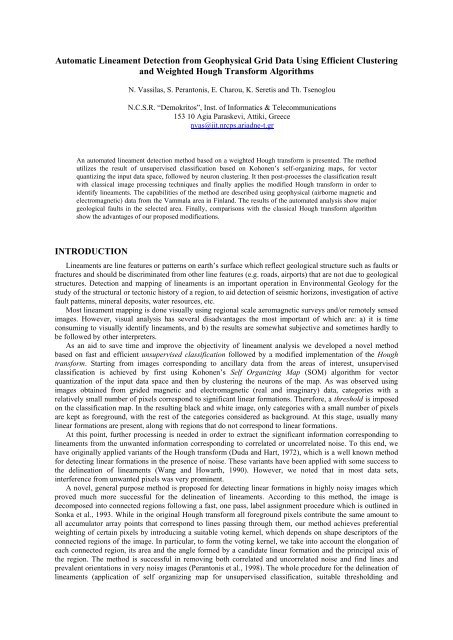
Automatic Lineament Detection from Geophysical Grid Data Using Efficient Clusteringand Weighted Hough Transform AlgorithmsN. Vassilas, S. Perantonis, E. Charou, K. Seretis and Th. TsenoglouN.C.S.R. “Demokritos”, Inst. of Informatics & Telecommunications153 10 Agia Paraskevi, Attiki, Greecenvas@iit.nrcps.ariadne-t.grAn automated lineament detection method based on a weighted Hough transform is presented. The methodutilizes the result of unsupervised classification based on Kohonen’s self-organizing maps, for vectorquantizing the input data space, followed by neuron clustering. It then post-processes the classification resultwith classical image processing techniques and finally applies the modified Hough transform in order toidentify lineaments. The capabilities of the method are described using geophysical (airborne magnetic andelectromagnetic) data from the Vammala area in Finland. The results of the automated analysis show majorgeological faults in the selected area. Finally, comparisons with the classical Hough transform algorithmshow the advantages of our proposed modifications.INTRODUCTIONLineaments are line features or patterns on earth’s surface which reflect geological structure such as faults orfractures and should be discriminated from other line features (e.g. roads, airports) that are not due to geologicalstructures. Detection and mapping of lineaments is an important operation in Environmental Geology for thestudy of the structural or tectonic history of a region, to aid detection of seismic horizons, investigation of activefault patterns, mineral deposits, water resources, etc.Most lineament mapping is done visually using regional scale aeromagnetic surveys and/or remotely sensedimages. However, visual analysis has several disadvantages the most important of which are: a) it is timeconsuming to visually identify lineaments, and b) the results are somewhat subjective and sometimes hardly tobe followed by other interpreters.As an aid to save time and improve the objectivity of lineament analysis we developed a novel methodbased on fast and efficient unsupervised classification followed by a modified implementation of the Houghtransform. Starting from images corresponding to ancillary data from the areas of interest, unsupervisedclassification is achieved by first using Kohonen’s Self Organizing Map (SOM) algorithm for vectorquantization of the input data space and then by clustering the neurons of the map. As was observed usingimages obtained from grided magnetic and electromagnetic (real and imaginary) data, categories with arelatively small number of pixels correspond to significant linear formations. Therefore, a threshold is imposedon the classification map. In the resulting black and white image, only categories with a small number of pixelsare kept as foreground, with the rest of the categories considered as background. At this stage, usually manylinear formations are present, along with regions that do not correspond to linear formations.At this point, further processing is needed in order to extract the significant information corresponding tolineaments from the unwanted information corresponding to correlated or uncorrelated noise. To this end, wehave originally applied variants of the Hough transform (Duda and Hart, 1972), which is a well known methodfor detecting linear formations in the presence of noise. These variants have been applied with some success tothe delineation of lineaments (Wang and Howarth, 1990). However, we noted that in most data sets,interference from unwanted pixels was very prominent.A novel, general purpose method is proposed for detecting linear formations in highly noisy images whichproved much more successful for the delineation of lineaments. According to this method, the image isdecomposed into connected regions following a fast, one pass, label assignment procedure which is outlined inSonka et al., 1993. While in the original Hough transform all foreground pixels contribute the same amount toall accumulator array points that correspond to lines passing through them, our method achieves preferentialweighting of certain pixels by introducing a suitable voting kernel, which depends on shape descriptors of theconnected regions of the image. In particular, to form the voting kernel, we take into account the elongation ofeach connected region, its area and the angle formed by a candidate linear formation and the principal axis ofthe region. The method is successful in removing both correlated and uncorrelated noise and find lines andprevalent orientations in very noisy images (Perantonis et al., 1998). The whole procedure for the delineation oflineaments (application of self organizing map for unsupervised classification, suitable thresholding and

application of the novel line detection method) is outlined in Figure 1. The major steps of this approach areanalyzed in the subsequent sections.Data (images or grid data)Unsupervised classificationThresholdingConnected region identificationEvaluation of shape descriptorsApplication of weighted Hough TransformLineamentsFigure 1: Outline of the procedure for the delineation of lineaments.UNSUPERVISED CLASSIFICATIONA new methodology for efficient clustering and automatic classification of images or grided spatial data wasused (Vassilas and Charou, 1999; Vassilas et al., 1999). Significant clustering and classification speedup wasachieved by: a) using a self-organizing map for vector quantization of the data space, b) clustering the neuronsof the map instead of the pixels of the original image, and c) using fast indexing techniques for efficientclassification. Moreover, the computational speedup allows the user to optimize the results through repeatedclassifications with different number of clusters each time. Application of the proposed methodology toaeromagnetic and satellite images shows speedup of several orders of magnitude with respect to conventionalclustering and classification techniques with no significant loss in terms of final performance.The unsupervised classification techniques are mainly used when no training sets are available andconstitute a valuable objective alternative since they do not depend on previous knowledge andphotointerpreter’s experience. These techniques, first cluster the data according to some similarity criterion,then assign a label to each cluster (usually a gray level or color) that corresponds to a (thematic) category and,finally, substitute each pixel of the original image with the cluster label to which it belongs (Figure 2). Amongthe most popular statistical clustering algorithms, we mention the Isodata algorithm (Duda and Hart, 1973) andthose based on statistical analysis of multidimensional histograms (Goldberg and Shlien, 1978). It is worth

noticing that a number of other statistical clustering algorithms, such as the various hierarchical algorithms(Duda and Hart, 1973) and algorithms based on scale-space analysis (Wong and Posner, 1993) can not be usedin applications involving large volumes of data due to their computational complexity. As far as the nonconventional algorithms are concerned, we mention the Fuzzy Isodata algorithm (Bezdeck, 1981; Cannon et al.,1986) from the fuzzy logic discipline and the neural algorithms such as the self-organizing maps (Cappellini etal., 1995; Kohonen,1989), a variant of the Adaptive Resonance Theory (ART) neural network (Baraldi andParmiggiani, 1995) and the hybrid BatchMap algorithm (Kohonen, 1995).Images orGrid dataClusteringThematicMapFigure 2: Traditional automatic classification.Kohonen's self-organizing maps (SOM) (Kohonen, 1989; Kohonen, 1995; Ienne et al., 1997), is one of themost popular neural algorithms for clustering and vector quantization. SOM is a competitive algorithm used forunsupervised training of single-layered neural networks (1-D or usually 2-D lattices of neurons), whereby, asequence of inputs is randomly presented to the network (map) and its weights are then updated so as toreproduce the input probability distribution as closely as possible. The weights self-organize in the sense thatneighboring neurons respond to neighboring inputs (topology preserving mapping of the input space to theneurons of the map) and tend toward asymptotic values that quantize the input space in an optimal way. Usingthe Euclidean distance metric, the SOM algorithm performs a Voronoi tessellation of the input space (Kohonen,1989; Kohonen, 1995) and the asymptotic weight vectors can then be considered as a catalogue ofrepresentatives or prototypes, with each such prototype representing all data from its corresponding Voronoicell.In the sequel, we present our methodology for automatic classification with the following advantages: a)memory savings through data quantization, b) clustering speedup, due to the relatively small number ofprototypes, allowing the use of even the most computationally demanding algorithms, and c) classificationspeedup by using fast indexing techniques. For the presentation, we will assume MxN images obtained from ngrided data sets. The input space R n is used to represent the image as a set of MxN points whose coordinates arethe corresponding values of each data set.The first stage of the proposed methodology involves vector quantization of the input space using a 2-Dlattice of neurons trained with the SOM algorithm. Following a random presentation of these n-dimensionalpoints, the result is to obtain a catalogue of prototypes (the asymptotic weights of the neurons) that quantize theimage.Next, we use indexing techniques for mapping the pixels of the original image to their correspondingprototypes. To this end, an MxN index table is constructed to store pointers from pixels to their closestprototypes. The replacement of the original image with the catalogue of prototypes and the index table (Figure3) constitutes the indexed representation of the image and results not only in data compression but also in asignificant speedup of both data clustering and classification.In general, the larger the number of neurons of the map is, the better the approximation of the original dataspace will be, due to a smaller quantization distortion (provided that the map self-organizes). However,according to experience, map sizes of no more than 16x16 neurons should suffice in most applications. In thecase of large volumes of data from n data sets with 256 values/data set, compression ratios of approximatelyn:1, when 256 prototypes are used, are readily attainable.Typically, automatic classification involves clustering of the data space followed by label assignment.However, due to the large number of data points (up to MxN different values), clustering performed on theoriginal image data is inefficient in terms of both memory and time requirements. On the other hand, in ourmethodology clustering is performed on the neurons of the map (i.e., the catalogue of prototypes), thus,achieving orders of magnitude a speedup, allowing us to use even the most computationally complex methods

Images orGrid dataSOMCatalogueof SOMPrototypesIndexTableFigure 3: Indexed representation.such as the hierarchical algorithms (Duda and Hart, 1973). Following clustering, the next step assigns labels toeach cluster. These clusters along with their labels will represent the automatic classification categories. At thefinal stage of the proposed methodology, first the catalogue of prototypes is classified to obtain a correspondingcatalogue of labels (Figure 4) and then by using fast indirect addressing through the index table (its pointers tothe prototypes also point to their labels) the final classification result (thematic map) is obtained (Figure 5).Catalogueof SOMPrototypesClusteringCatalogueofLabelsFigure 4: Creation of the catalogue of labels.CatalogueofLabelsThematicMapIndexTableFigure 5: Fast indexed classification

THRESHOLDING OF THE CLASSIFICATION RESULTA thresholding method was used as the binarization method of the classified image. A histogram of theimage is plotted in order to assist on the specification of one of the four following thresholding methods: Percentage Threshold (0-100%): Gray levels whose percentage of pixels with respect to the total number ofpixels in the image are below the threshold, are assigned to the foreground. Otherwise they are assigned tothe background. Gray Level Threshold (0-255): This is the traditional thresholding method in image processing. All graylevels above the threshold are assigned to foreground, otherwise, they are assigned to background. Foreground Gray Levels: Explicitly defined values of grays to be assigned to foreground. Background Gray Levels: Explicitly defined values of grays to be assigned to background.CONNECTED REGION IDENTIFICATION - SHAPE DESCRIPTOR EVALUATIONThe connected regions of the binary image were specified by using the label assignment procedure outlinedin (Sonka et al., 1993), whereby a linked list is constructed for storing simultaneously the following:1. labels belonging to different regions using vertical pointers, and2. equivalence classes, i.e., labels assigned to pixels of the same region using horizontal pointers.The image is scanned top to bottom and left to right, skipping background pixels, until a new foregroundpixel is found. If all the top and left connected neighbors (e.g. assuming 4- or 8-connectedness) belong to thebackground, a new label is added to the bottom of the linked list and the pixel points to this label (the pointersfrom pixels to labels are stored in a 2-D array with the same dimensions as the original image). Otherwise, thepixel is made to point to the first label found among the foreground top and left neighbors. Inconsistencies dueto two different neighboring pixels having different labels are easily resolved as follows: the second found labelis first removed from the vertical label list, then placed to the equivalence class (horizontal list) of the firstfound label and finally changed to the first found label (also specifying the equivalence class). Such a techniquehas the advantage of speed, since it does not require a second image scanning in order to assure uniformity inregion labeling, i.e., changing all equivalent labels to one.For each connected region we then calculate three shape descriptors, all of which can be evaluated in termsof the central moments m ij of the region:1. The area:A = m 00 . (1)2. The angle of the principal axis relative to the x-axis, given by the equation: =12tan -1 [2 m 11 /(m 20 - m 02 )]). (2)3. The elongation of the region. This is evaluated by finding the ellipse that best fits the region (in the sensethat it has the same moments of inertia). The elongation ε is then equal to the major to minor axis lengthratio (so that ε > 1) and can be found as:whereandε = | I max /I min | 1/2 , (3)I min = m 20 sin 2 + m 02 cos 2 - m 11 sin2 (4)I max = m 20 cos 2 + m 02 sin 2 + m 11 sin2. (5)Details on the derivation of these formulae can be found in (Jain, 1989).

MODIFIED HOUGH TRANSFORMThe Hough transform is a popular and powerful method for detecting parametrically described shapes inimages. However, even in its simplest application, which is the detection of straight lines, the original Houghtransform is susceptible to the presence of both random and correlated noise that may give rise to spuriousmaxima in the accumulator array (Leavers, 1993). The problem is especially acute in cases where the requiredlines are axes located in the interior of objects, so that edge detection followed by Hough transform applicationis not appropriate for locating them (Gatos et al., 1996). It is thus highly desirable to have methods of hinderingirrelevant pixels from contributing to the accumulator array. In the original Hough transform all foregroundpixels contribute the same amount to all accumulator array points that correspond to lines passing through them.Preferential weighting of certain pixels can be achieved by introducing a voting kernel (Palmer et al., 1997).Here we present a novel method that employs a suitably defined voting kernel to reduce interference effects andavoid spurious accumulator array maxima even in very noisy images. The kernel depends on the shapedescriptors of the connected regions of the image described in the previous section. The method is highlysuccessful in finding linear directions in demanding image processing and computer vision applications.Given a binary image, we are interested in the detection of straight lines whose points (x,y) areparameterized by r = x cos + y sin, where r is the distance of the origin from a particular line and is theangle formed by the normal to the line and the x-axis (Figure 6). For each connected region, we consider itsgeometrical center and increment for various values of θ the corresponding cells in the accumulator array. Toevaluate the contribution of each region to various cells in the accumulator array we take into account its relatedshape descriptors and express the dependence formally by introducing a voting kernel.θxryFigure 6: Parametrization of a straight line for application of Hough transform.The voting kernel is a continuous function of the shape descriptors and is constructed by taking into accountthe following considerations. The presence of an elongated region is taken as strong evidence for the existenceof a line parallel to the principal axis of the region. Thus, the contribution to the accumulator array shouldincrease with ε. Moreover, for a given value of ε, this contribution should be maximum for = and drop withincreasing | - |. The rate of change with increasing | - | should clearly depend on ε. For very elongatedregions, only the direction = should be incremented. On the other hand, nearly circular regions (ε 1)should be allowed to vote equally for all directions. Finally, a dependence of the kernel on the area A should beintroduced in order to minimize interference effects and avoid spurious accumulator array maxima.Contributions from regions of large A and relatively small ε should be suppressed. These regions are a majorsource of correlated noise, because spurious lines can be formed from points lying in their interior. At the otherextreme, regions of very small A should also be discarded as random noise. In-between these extreme cases,regions of small ε whose area is comparable to a characteristic intermediate area scale A 0 may be part of a chainof regions contributing to a disrupted linear structure and should be taken into account.To summarize, given a connected region whose center is located at (x _ , y _ ) and a value of the angle , thecontribution to the accumulator array cell (r, ) is of the form f (A, ε, - ) where f must fulfill the followingconditions:1. should be asymptotically proportional to ε as ε 2. f should not depend on as ε 1 and should tend to ( - ) as ε 3. for ε 1, we should have f 0 as A 0 or A The following function is modeled to conform with the above conditions:

f = ε exp[ - (ε - 1) ( - ) 2 ] A exp[ - (Α – Α 0 )/(Α 0 ε 2 )] (6)The factor ε weights elongated regions in accordance with condition 1; the factor exp[ - (ε - 1) ( - ) 2 ] isinserted to conform with condition 2; and the factor A exp[ - (Α – Α 0 )/(Α 0 ε 2 )], which has a maximum at A = A 0for given ε, plays the role of a band-pass filter for values of ε close to 1 (so that condition 3 is fulfilled). A 0 canbe chosen as the average area of regions whose elongation exceeds a threshold. However, our simulations haveshown that the method is robust, exhibiting stable performance for a wide range of values for A 0 .EXPERIMENTAL RESULTS AND DISCUSSIONThe automatic lineament detection method has been applied with success on different combinations ofgeophysical airborne magnetic and electromagnetic (real and imaginary) data from the Vammala area inFinland. For visualization purposes, the original 601x801 grid data were first linearly mapped in [0, 255], thenquantized to the nearest integer and finally shown as images. In the sequel, we show the results produced by acombination of magnetic and real electromagnetic data (Figures 7a and 7b).All programs were run on a SUN ULTRA II Enterprise workstation (64MB, 167MHz). A map of 16x16neurons was trained with 10 5 random presentations of the 2-D grid data in 20.35sec. Following SOM training,the storage of asymptotic weights into the catalogue of SOM prototypes (256 prototypes x 2 floats/prototype x 4bytes/float x 8 bits/byte = 2 14 bits) and the index table construction (601 x 801 indices x 8 bits/index 1.8 x 2 21bits) required 87.06sec. The SOFM prototypes and index table can also be used for representing the originaldata (2 data sets x 601 x 801 integers/data set x 32 bits/integer 1.8 x 2 24 bits) in a compressed form. Thecompression ratio achieved in this case is about 8 while higher ratios can be obtained for more data sets and/orsmaller maps, although, caution should be exercised with the latter since small maps may lead to largequantization distortions.Automatic classification in 10 categories was then performed by clustering the neurons of the map using theFuzzy Isodata algorithm. The algorithm was terminated after a preselected maximum number of 100 iterationsin 0.58sec and the classification result is shown in Figure 8a. The additional indexed classification time was0.40sec. Direct application of the Fuzzy Isodata algorithm to the original data is possible at a cost of about 1880times (601x801/256) longer clustering time per iteration. In fact, original data clustering in 10 categoriesrequired 1153.34 sec (100 iterations) while classification required 3.75sec.From the above, the clustering speedup per iteration, achieved by using the proposed methodology withFuzzy Isodata, is about 1153.34/0.58 = 1988 while the classification speedup, due to the indexing techniques,was 3.75/0.4 = 9.375. At this point, it is important to notice that if SOM training and index table construction(requiring 107.41sec) are not off-line computations, the speedup in the first user trial will be smaller. However,for any additional classification trials (with different number of clusters) performed by the user for optimizingthe results, the speedup will be as stated above.Following unsupervised classification, the image is then binarized in 0.03sec using a variant of the firstthresholding criterion, whereby, the foreground pixels inlude the smallest categories that cummulatively do notexceed 20% of the total image area (see Figure 8b). The 8-neighbors connected regions along with the area,principal axis angle and elongation shape descriptors of each region are then computed in 0.67sec. Finally, thelineaments are found using the proposed weighted Hough transform in 5.96sec and are shown superimposed onthe binarized classification result in Figure 9a.Figure 9b shows the lineaments found by the original Hough method superimposed on the binarizedclassification result. It is apparent that interference from unwanted pixels (mainly from the large regions foundin the bottom of the image) was very prominent and that this method fails to delineate lineaments. On the otherhand, the result obtained with the proposed (modified) Hough transform following extraction of the appropriateshape descriptors clearly shows significant linear formations (see Figure 9a). Similar results are also obtainedby applying the original Hough transform to the image of Figure 10a which contains the edges of the binarizedclassification result. As most of the edge pixels lie in the bottom of the image, the method fails to detect the truelinear formations (see Figure 10b).In short, we believe that our proposed method for automatic lineament detection can prove a useful tool notonly to those involved with environmental informatics but also to geologists and geophysicists who would liketo have a first glance on a digital lineament map without significant time investment. Such a map can then serveas the starting map of a series of improved lineament maps produced within a Geographical Information System(GIS), whereby, existing lineaments can be modified, new ones added and wrong ones removed, by the use ofpointing devices, incorporating additional geological and/or geophysical information.

(a)(b)Figure 7: Original geophysical grid data from Vammala area visualized as 601x801 gray level images:(a) magnetic data, (b) real part of electromagnetic data.(a)(b)Figure 8: (a) Classification result in 10 categories using a self-organizing map and Fuzzy Isodata neuronclustering, and (b) binarized classification result.(a)(b)Figure 9: Lineament detection from the Vammala area, superimposed on thresholded classification result using(a) the modified Hough transform, and (b) the original Hough transform.

(a)(b)Figure 10: (a) Binary image produced by extracting the edges of Figure 8b, and (b) the most prominent linesfound by the original Hough transform.AcknowledgmentThe authors would like to thank Dr. Soininen, Dr. Markku and Dr. Gustavsson all from the GeophysicalSurvey of Finland who so kindly provided us with the Vammala geophysical data.REFERENCESBaraldi, A. and Parmiggiani, F., 1995, “A Neural Network for Unsupervised Categorization of MultivaluedInput Patterns: An Application to Satellite Image Clustering”, IEEE Trans. on Geoscience and RemoteSensing, Vol. 33, No. 2, pp. 305-316.Bezdek, J.C., 1981. Pattern Recognition with Fuzzy Objective Function Algorithms. New York: Plenum Press.Cannon, R.L., Dave, J.V., Bezdek, J.C. and Trivedi, M.M., 1986, “Segmentation of a Thematic Mapper ImageUsing the Fuzzy c-Means.Clustering Algorithm”, IEEE Trans. on Geoscience and Remote Sensing, Vol. 24,No. 3, pp. 400-408.Cappellini, V., Chiuderi, A. and Fini, S., 1995, “Neural Networks in Remote Sensing Multisensor DataProcessing”, in Proceedings 14th EARSeL Symposium'94 (Sensors and Environmental Applications ofRemote Sensing), J. Askne (ed.), Rotterdam: A.A. Balkema, Geteborg, pp. 457-462.Duda, R. O. and Hart, P.E., 1972, “Use of the Hough Transform to Detect Lines and Curves in Pictures”,Communications of the ACM, Vol. 15, pp. 11-15.Duda, R.O. and Hart, P.E., 1973. Pattern Classification and Scene Analysis. New York: Wiley.Gatos, B., Perantonis, S.J. and Papamarkos, N., 1996, “Accelerated Hough Transform Using Rectangular ImageDecomposition”, Electronics Letters, Vol. 32, No. 8, pp. 730-732.Goldberg, M. and Shlien, S., 1978, “A Clustering Scheme for Multispectral Images”, IEEE Transactions onSystems, Man, and Cybernetics, Vol. 8, No. 2, pp. 86-92.Ienne, P., Thiran, P. and Vassilas, N., 1997, “Modified Self-Organizing Feature Map Algorithms for EfficientDigital Hardware Implementation”, IEEE Trans. on Neural Networks, Vol. 8, No. 2, pp. 315-33.Kohonen, T., 1989. Self-Organization and Associative Memory. 3 rd ed., Berlin-Heidelberg-New York: SpringerVerlag.Kohonen, T., 1995. Self-Organizing Maps. Berlin-Heidelberg-New York: Springer Verlag.Leavers, V.F., 1993, “Which Hough Transform?”, Computer Vision and Image Understanding, Vol 58, No. 2,pp. 250-264.Palmer, P.L, Kittler, J. and Petrou, M., 1997, “An Optimizing Line Finder Using a Hough TransformAlgorithm”, Computer Vision and Image Understanding, Vol. 67, No. 1, pp. 1-23.Perantonis, S. J., Vassilas, N., Tsenoglou, Th. and Seretis, K., 1998, “Robust Line Detection Using WeightedRegion Based Hough Transform”, Electronics Letters, Vol. 34, No. 7, pp. 648-650.Sonka, M., Hlavac, V. and Boyle, R., 1993. Image Processing, Analysis and Machine Vision. London:Chapman and Hall, pp 197-198.Vassilas, N. and Charou, E., 1999, “A New Methodology for Efficient Classification of Multispectral SatelliteImages Using Neural Network Techniques”, Neural Processing Letters, Vol. 9, pp. 35-43.

Vassilas, N., Vaiopoulos, D., Charou, E. and Varoufakis, S., 1999, “Efficient Satellite Image Clustering andClassification in Land-Cover Categories Using Self-Organizing Maps”, Technical Chronicles - ScientificEdition of the Technical Chamber of Greece. In print.Wang, J. and Howarth, P.J., 1990, “Use of the Hough transform in automated lineament detection”, IEEETransactions on Geoscience and Remote Sensing, Vol. 28, No. 4, pp. 561-566.Wong, Y.-F. and Posner, E.C., 1993, “A New Clustering Algorithm Applicable to Multispectral andPolarimetric SAR Images”, IEEE Trans. on Geoscience and Remote Sensing, Vol. 31, No. 3, pp. 634-644.