Compile-time Loop Splitting for Distributed Memory ... - Stanford AI Lab

J=100
I=100
0 1
2 3
A
0
1
2
3
B
0 1 2 3
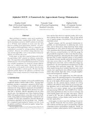
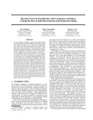
Figure 2-4: Three examples of data partitioning for a 100x100 array on four processors:
(a) blocking, (b) striping by rows, and (c) striping by columns. The numbers designate
assignment of the array portions to the virtual processors.
2.2.2 Data Partitioning
While the task is divided among processors for all parallel machines, the data of a program
is divided only on a distributed memory multiprocessor. In a distributed memory system,
every memory address is local to some processor node; and every processor node has its
own piece of memory, from which all nodes may read and to which all may write. The data
structure relevant to data partitioning is the array and is distributed among the memories
without duplication. Figure 2-4 shows several data distributions for a 2-D array, each with
a different mapping of the array onto the processor memories.
Figure 2-4 helps to define more terms. First, the data spread is the dimension length
of the data portion located in a processor’s memory. In Figure 2-4a both the � ����—�and
� ����—�are 50 array elements each; in Figure 2-4b, � ����—�is 100 elements and � ����—�
is 25; and in Figure 2-4c � ����—�is 25 elements and � ����—�is 100. Second, the virtual
network is the arrangement of the virtual processors on which alignment maps the data.
This virtual network is then mapped onto the (possibly different) real network of physical
processors by a procedure called placement. The dimensions of the virtual network play an
important role in array referencing (explained in Section 2.5) and are called � ���, where
�is the dimension name. In Figure 2-4a, both the � ��� and � ��� are 2 virtual
processors; in Figure 2-4b � ��� is 1 and � ��� is 4; and in Figure 2-4c � ��� is 4
processors and � ��� is 1.
Like task partitioning, the ideal data partitioning distributes equal amounts of data
18
C