- Page 1: Real Options "in" Projects and Syst
- Page 4 and 5: 4Committee Member: Dr. David H. Mar
- Page 6 and 7: 6Table of Contents:Acknowledgements
- Page 8 and 9: 84.4.3. Binomial Tree______________
- Page 10 and 11: 108.7. Contributions and Conclusion
- Page 12 and 13: 12Figure 5-3: Scenario tree _______
- Page 14 and 15: 14Table 6-12 Sources of options val
- Page 16 and 17: 16fFC s∆F sthiH sh tThe ratio of
- Page 18 and 19: 18X styyY jYYjAverage flow from sit
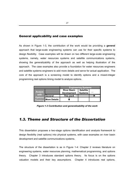
- Page 20 and 21: 201.1. The problemWith the recognit
- Page 22 and 23: 22The first thread - engineering sy
- Page 24 and 25: 24The second thread - options theor
- Page 28 and 29: 28especially the difference between
- Page 30 and 31: 30every area in a more and more det
- Page 32 and 33: 32made between forecasts of the lev
- Page 34 and 35: 34memory (whereas modern computers
- Page 36 and 37: 36model and presented a multiple-yi
- Page 38 and 39: 38such designs exist) by simply rec
- Page 40: 40mathematical properties of maximi
- Page 43 and 44: 43that incorporates important perfo
- Page 45 and 46: 45Dixit and Pindyck (1994) stressed
- Page 47 and 48: 47The real options “in projects
- Page 49 and 50: 491980s, Merck began to use simulat
- Page 51 and 52: 51that the integrated approach (the
- Page 53 and 54: 53blurs the exercise condition, bec
- Page 55 and 56: 55Goldberg and Read (2000) found th
- Page 57 and 58: 57In general, real options “in”
- Page 59 and 60: 59- And, mathematical programming,
- Page 61 and 62: 61Example of a stock call option:Jo
- Page 63 and 64: 63or $300. Arbitrage opportunities
- Page 65 and 66: 659 × 0.25 =2.25Regardless of whet
- Page 67 and 68: 67∆Z = ε ∆twhere ε denotes a
- Page 69 and 70: 69standard deviation of 1.0. It fol
- Page 71 and 72: 71price rather than as a function o
- Page 73 and 74: 73The stock price process is the on
- Page 75 and 76: 75Equation 3-9 is the Black-Scholes
- Page 77 and 78:
7710,000 Trials Frequency Chart90 O
- Page 79 and 80:
79The two are equal whenorS0ux− f
- Page 81 and 82:
81S uuS uf uuS f u S udfS df udf dS
- Page 83 and 84:
83Figure 3-10 Decision Tree for Opt
- Page 85 and 86:
85the Black-Scholes formula is $1.9
- Page 87 and 88:
87The expected growth of the stock
- Page 89 and 90:
89option, the holder has the right
- Page 91 and 92:
91Boston expects to receive a cash
- Page 93 and 94:
93the value of a European put on a
- Page 95 and 96:
95Chapter 4 Real Options“The clas
- Page 97 and 98:
97In addition to understanding the
- Page 99 and 100:
99gas. The development was unsucces
- Page 101 and 102:
101But if we employ Real Options th
- Page 103 and 104:
103Option to switch (e.g.,outputs o
- Page 105 and 106:
105The fifth step, by comparing the
- Page 107 and 108:
107Real Options "in" ProjectsReal O
- Page 109 and 110:
109- 5 and 3.5 billion dollars resp
- Page 111 and 112:
111Real options “on” projectsVa
- Page 113 and 114:
1134.3.4. A Case Example on analysi
- Page 115 and 116:
115Step 1: Table 4-6 illustrates th
- Page 117 and 118:
11710EXPECTED NPV ($, MILLIONS)50-5
- Page 119 and 120:
119PROBABILITY1.00.90.80.70.60.50.4
- Page 121 and 122:
1214.4.1. Black-Scholes FormulaAs d
- Page 123 and 124:
123and buy the real options to earn
- Page 125 and 126:
125computationally prohibitive to c
- Page 127 and 128:
1274.5. Some Implications of Real O
- Page 129 and 130:
129Value of flexibility Appropriate
- Page 131 and 132:
1314.6.2. What is the definition of
- Page 133 and 134:
133- It aims at an expected value o
- Page 135 and 136:
135Chapter 5 Valuation of Real Opti
- Page 137 and 138:
137uncertain environment. Specifica
- Page 139 and 140:
139assuming steady state, i.e. all
- Page 141 and 142:
141modify this standard simulation
- Page 143 and 144:
143Table 5-1: Decision on each node
- Page 145 and 146:
145The objective function is to get
- Page 147 and 148:
1475.3.2. Stochastic mixed-integer
- Page 149 and 150:
149q⎛ R ⎞1⎜ ⎟qR = ⎜ ...
- Page 151 and 152:
151Table 5-4: Stochastic programmin
- Page 153 and 154:
153The real options timing model fo
- Page 155 and 156:
1555.4. A case example on satellite
- Page 157 and 158:
157Table 5-6 Evolution of demand fo
- Page 159 and 160:
1595.4.3. ParametersWe consider thr
- Page 161 and 162:
161Year 0 Year 2.5 Year 5 Year 7.5
- Page 163 and 164:
163scenario trees based on better s
- Page 165 and 166:
165The total length of the river is
- Page 167 and 168:
167Project 1 or 3. A shallow gradie
- Page 169 and 170:
169Table 6-5: Stream flow for Proje
- Page 171 and 172:
171The reservoir cost coefficient a
- Page 173 and 174:
173Q in,tQ in,tProject CSite 3Site
- Page 175 and 176:
175k t= (60Sec/ Min)× (60Min/ Hour
- Page 177 and 178:
177Reservoir cost: α ( Vss) = FCs+
- Page 179 and 180:
179[Power plant cost curve]δ 1 is
- Page 181 and 182:
181Complete formulation of the scre
- Page 183 and 184:
183Table 6-9 List of Parameters for
- Page 185 and 186:
185Step 1. The important uncertain
- Page 187 and 188:
187From the tornado diagram, we und
- Page 189 and 190:
189design feature where we consider
- Page 191 and 192:
191Table 6-13 List of design variab
- Page 193 and 194:
193Table 6-15 List of Parameters fo
- Page 195 and 196:
195A Realization Path of Electricit
- Page 197 and 198:
197Case II: there is enough water t
- Page 199 and 200:
199where the average head*Astis cal
- Page 201 and 202:
201Ball©. All designs from the scr
- Page 203 and 204:
203options sees Table 6-17. This is
- Page 205 and 206:
205XX= Q + Y ∑ Ri31 in,131 j331 i
- Page 207 and 208:
207Objective functionThe objective
- Page 209 and 210:
209According to the screening model
- Page 211 and 212:
211The hydropower benefit coefficie
- Page 213 and 214:
213Table 6-19 List of parameters fo
- Page 215 and 216:
215time to build and gradually incr
- Page 217 and 218:
217example, at year 20, if the pric
- Page 219 and 220:
219from 1 to 8. The hydropower bene
- Page 221 and 222:
221Our planning horizon is three st
- Page 223 and 224:
2235 6 7 82s= R2s= R2sR2sR =1 23sR3
- Page 225 and 226:
225yrsIndicating whether or not the
- Page 227 and 228:
227The overall expected net benefit
- Page 229 and 230:
229contingency plan is to build Pro
- Page 231 and 232:
231Table 6-26 Different water flow
- Page 233 and 234:
233Chapter 7 Policy Implications -O
- Page 235 and 236:
235excess water when water is more
- Page 237 and 238:
237The options methodology develops
- Page 239 and 240:
2397.2.2. Organizational Wisdom to
- Page 241 and 242:
241success. In the bank, the author
- Page 243 and 244:
243method. Sensitivity analysis wit
- Page 245 and 246:
245Chapter 8 Summary and Conclusion
- Page 247 and 248:
2478.2. Real options “in” proje
- Page 249 and 250:
249Note the difference between real
- Page 251 and 252:
251Carlo simulation model to value
- Page 253 and 254:
2538.3.1. Options identificationFor
- Page 255 and 256:
255can catch upside of the uncertai
- Page 257 and 258:
257where r is the drift rate (in th
- Page 259 and 260:
259A joint realization of the probl
- Page 261 and 262:
261Note there is an exercise in sce
- Page 263 and 264:
263The real options decision variab
- Page 265 and 266:
265development case example, we sim
- Page 267 and 268:
267The standard deviation of the co
- Page 269 and 270:
269reservoir fixed cost is less und
- Page 271 and 272:
271time series of the water flow co
- Page 273 and 274:
273Table 8-8 Configurations set Y f
- Page 275 and 276:
275Table 8-9: Results for real opti
- Page 277 and 278:
277inconvenient features and high c
- Page 279 and 280:
279Year 0 Year 2.5 Year 5 Year 7.5
- Page 281 and 282:
281Following is a report on the com
- Page 283 and 284:
283can be found in Chapter 6, whose
- Page 285 and 286:
285This dissertation has successful
- Page 287 and 288:
2878.7. Contributions and Conclusio
- Page 289 and 290:
289ReferencesAberdein, D. A. (1994)
- Page 291 and 292:
291Copeland, T.E. and Antikarov, V.
- Page 293 and 294:
293Jacoby, H.D. and Loucks, D. (197
- Page 295 and 296:
295Mason, S.P. and Merton, R.C. (19
- Page 297 and 298:
297Schoenberger, C. R. (2000) “Si
- Page 299 and 300:
299AppendicesAppendix 3A: Ito’s L
- Page 301 and 302:
301p;Binary variablesX(i,j);X.l('4'
- Page 303 and 304:
303Appendix 5B: GAMS Code for Ameri
- Page 305 and 306:
305n5 non-antipativity constraint 5
- Page 307 and 308:
3072 0.50 1.51 4.57 7.5 4.573 0.50
- Page 309 and 310:
309R(q,i,s)RTD(q,i,s)P1(q,i)P2(q,i)
- Page 311 and 312:
311na28na29na30na31na32na33na34na35
- Page 313 and 314:
313na26(s)..na27(s)..R('14','3',s)
- Page 315 and 316:
315Table DeltaF(s,t)1 21 0 02 0 03
- Page 317 and 318:
317EquationsObjBeneCostCont1Cont2Co
- Page 319 and 320:
319Appendix 6B: GAMS code for the t
- Page 321 and 322:
3213 -63.6 63.6;Scalars f /0.226/;P
- Page 323 and 324:
323Hydro1Hydro2Budget;*costs and be
- Page 325 and 326:
325Scalars es /0.7/;Scalars Kt /15.
- Page 327 and 328:
327VariablesXstiq(s,t,i,q)Pstiq(s,t
- Page 329 and 330:
329f)*Rsiq(s,i,'1') )))))*0.001 + P
- Page 331 and 332:
331Appendix 6D: GAMS code for real
- Page 333 and 334:
3331 2 31 9600 9600 96002 0 0 03 95
- Page 335 and 336:
335Rsiq.l('1','3','4') = 0;Rsiq.l('
- Page 337:
337Cont1(i,q).. Xstiq('3','1',i,q)