PLDA+: Parallel Latent Dirichlet Allocation with Data Placement and ...

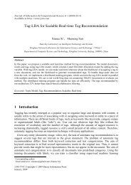
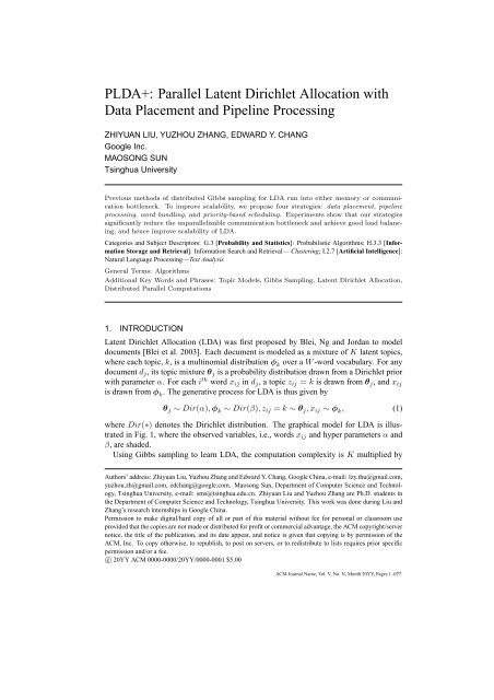
2 ·αθ jz ijβφ kKx ijN jDFig. 1: The graphical model for LDA.the total number of word occurrences in the training corpus. Prior work has exploredtwo main parallelization approaches for speeding up LDA: 1) parallelizing on looselycoupleddistributed computers, and 2) parallelizing on tightly-coupled multi-core CPUs orGPUs (Graphics Processing Units). Representative loosely-coupled distributed algorithmsare Dirichlet Compound Multinomial LDA (DCM-LDA) [Mimno and McCallum 2007],Approximate Distributed LDA (AD-LDA) [Newman et al. 2007], and Asynchronous DistributedLDA (AS-LDA) [Asuncion et al. 2008], which perform Gibbs sampling on computersthat do not share memory. This distributed approach may suffer from high intercomputercommunication cost, which limits achievable speedup. The tightly-coupled approachuses multi-core CPUs or GPUs with shared memory (e.g., the work of Yan, etal. [2009]). Such a shared-memory approach reduces inter-process communication time.However, once the processors and memory have been configured, the architecture is inflexiblewhen faced with changes in computation demands, and the need to schedule simultaneoustasks with mixed resource requirements. (We discuss related work in greater detailin Section 2.)In this work, we improve the scalability of the distributed approach by reducing intercomputercommunication time. Our algorithm, which we name PLDA+, employs fourinter-dependent strategies:(1) Data placement. Data placement aims to separate CPU-bound tasks and communicationboundtasks onto two sets of processors. Data placement enables us to employ apipeline scheme (discussed next), to mask communication by computation.(2) Pipeline processing. To ensure that a CPU-bound processor is not blocked by communication,PLDA+ conducts Gibbs sampling for a word bundle while performinginter-computer communication on the background. Suppose Gibbs sampling is performedon the words ‘foo’ and ‘bar’. PLDA+ fetches the metadata for the word ‘bar’while performing Gibbs sampling on the word ‘foo’. The communication time forfetching the metadata of ‘bar’ is masked by the computation time for sampling ‘foo’.(3) Word bundling. In order to ensure that communication time can be effectively masked,the CPU time must be long enough. Revisiting the example of sampling ‘foo’ and‘bar’, the CPU time for sampling the word ‘foo’ should be longer than the communicationtime for the word ‘bar’ in order to mask the communication time. Supposewe performed Gibbs sampling according to the order of words in documents, eachGibbs sampling time unit would be too short to mask the required communicationtime. Since LDA treats a document as a bag of words and entirely ignores word order,we can flexibly process words on a processor in any order without consideringACM Journal Name, Vol. V, No. N, Month 20YY.

· 3Table I: Symbols associated with LDA used in this paper.D Number of documents.K Number of topics.W Vocabulary size.N Number of words in the corpus.x ij Thei th word ind j document.z ij Topic assignment for wordx ij .C kj Number of topic k assigned tod j document.C wk Number of word w assigned to topick.C k Number of topic k in corpus.C doc Document-topic count matrix.C word Word-topic count matrix.C topic Topic count matrix.θ j Probability of topics given document d j .φ k Probability of words given topic k.α Dirichlet prior.β Dirichlet prior.P Number of processors.|P w| Number ofP w processors.|P d | Number ofP d processors.p i Thei th processor.document boundaries. Word bundling combines words into large computation units.(4) Priority-based scheduling. Data placement and word bundling are static allocationstrategies for improving pipeline performance. However, run time factors would almostalways affect the effectiveness of a static allocation scheme. Therefore, PLDA+employs a priority-based scheduling scheme to smooth out run-time bottlenecks.The above four strategies must work together to improve speedup. For instance, withoutword bundling, pipeline processing is futile because of short computation units. Withoutdistributing the metadata of word bundles, communication bottlenecks at the masterprocessor could cap scalability. By lengthening the computation units via word bundling,while shortening communication units via data placement, we can achieve more effectivepipeline processing. Finally, a priority-based scheduler helps smooth out unexpected runtimeimbalances in workload.The rest of the paper is organized as follows: We first present LDA and related distributedalgorithms in Section 2. In Section 2.3 we present PLDA, an MPI implementationof Approximate Distributed LDA (AD-LDA). In Section 3 we analyze the bottleneck ofPLDA and depict PLDA+. Section 4 demonstrates that the speedup of PLDA+ on largescaledocument collections significantly outperforms PLDA. Section 5 offers our concludingremarks. For the convenience of readers, we summarize the notations used in this paperin Table I.2. LDA OVERVIEWSimilar to most previous work [Griffiths and Steyvers 2004], we use symmetric Dirichletpriors in LDA for simplicity. Given the observed wordsx, the task of inference for LDA isto compute the posterior distribution of the latent topic assignments z, the topic mixturesof documents θ, and the topics φ.ACM Journal Name, Vol. V, No. N, Month 20YY.

4 ·2.1 LDA LearningGriffiths and Steyvers [2004] proposed using Gibbs sampling, a Markov-chain MonteCarlo (MCMC) method, to perform inference for LDA. By assuming a Dirichlet priorβ onφ,φcan be integrated (hence removed from the equation) using the Dirichlet-multinomialconjugacy. MCMC is widely used as an inference method for latent topic models, e.g.,Author-Topic Model [Rosen-Zvi et al. 2010], Pachinko Allocation [Li and McCallum2006], and Special Words with Background Model [Chemudugunta et al. 2007]. Moreover,since the memory requirement of VEM is not nearly as scalable as that of MCMC[Newman et al. 2009], most existing distributed methods for LDA use Gibbs samplingfor inference, e.g., DCM-LDA, AD-LDA, and AS-LDA. In this paper we focus on Gibbssampling for approximate inference. In Gibbs sampling, it is usual to integrate out the mixturesθand topicsφand just sample the latent variablesz. The process is called collapsing.When performing Gibbs sampling for LDA, we maintain two matrices: a word-topic countmatrix C word in which each element C wk is the number of word w assigned to topic k,and a document-topic count matrixC doc in which each elementC kj is the number of topick assigned to document d j . Moreover, we maintain a topic count vector C topic in whicheach element C k is the number of topic k assignments in document collection. Given thecurrent state of all but one variable z ij , the conditional probability of z ij iswk +βC ¬ijkp(z ij = k|z ¬ij ,x ¬ij ,x ij = w,α,β) ∝ C¬ij+Wβ( )C ¬ijkj+α , (2)where ¬ij means that the corresponding word is excluded in the counts. Whenever z ij isassigned with a new topic drawn from Eq. (2),C word ,C doc andC topic are updated. Afterenough sampling iterations to burn in the Markov chain, θ and φ are estimated.2.2 LDA Performance EnhancementVarious approaches have been explored for speeding up LDA. Relevant parallel methodsfor LDA include:—Mimno and McCallum [2007] proposed Dirichlet Compound Multinomial LDA (DCM-LDA), where the datasets are distributed to processors, Gibbs sampling is performedon each processor independently without any communication between processors, andfinally a global clustering of the topics is performed.—Newman, et al. [2007] proposed Approximate Distributed LDA (AD-LDA), where eachprocessor performs a local Gibbs sampling iteration followed by a global update usinga reduce-scatter operation. Since the Gibbs sampling on each processor is performedwith the local word-topic matrix, which is only updated at the end of each iteration, thismethod is called approximate distributed LDA.—In [Asuncion et al. 2008], a purely asynchronous distributed LDA was proposed, whereno global synchronization step like in [Newman et al. 2007] is required. Each processorperforms a local Gibbs sampling step followed by a step of communicating with otherrandom processors. In this paper we label this method as AS-LDA.—Yan, et al. [2009] proposed parallel algorithms of Gibbs sampling and VEM for LDAon GPUs. A GPU has massively built-in parallel processors with shared memory.Besides these parallelization techniques, the following optimizations can reduce LDAmodel learning computation cost:ACM Journal Name, Vol. V, No. N, Month 20YY.

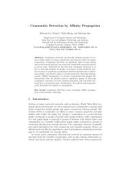
6 ·WKD/PWW/PwKD/PdW(A) PLDA(B) PLDA+Fig. 2: The assignments of documents and word-topic count matrix for PLDA and PLDA+.(A) PLDA(B) AS-LDA(C) PLDA+Pd1Root(P )KW KWKWP P P1 2 30P0KWP1PKW2Pd0KPwKKKPPd2d3Fig. 3: The spread patterns of the updated topic distribution of a word from one processor for PLDA, AS-LDAand PLDA+.3.1 Bottlenecks for PLDAAs presented in the previous section, in PLDA, D documents are distributed over P processorswith approximately D/P documents on each processor. This is shown with aD/P -by-W matrix in Fig. 2(A), where W indicates the vocabulary of document collection.The word-topic count matrix is also distributed, with each processor keeping a localcopy, which is theW -by-K matrix in Fig. 2(A).In PLDA, after each iteration of Gibbs sampling, local word-topic counts on each processorare globally synchronized. This synchronization process is expensive partly becausea large amount of data is sent and partly because the synchronization starts only when theslowest processor has completed its work. To avoid unnecessary delays, AS-LDA [Asuncionet al. 2008] does not perform global synchronization like PLDA. In AS-LDA a processoronly synchronizes word-topic counts with another finished processor. However, sinceword-topic counts can be outdated, the sampling process can take a larger number of iterationsthan that PLDA does to converge. Fig. 3(A) and Fig. 3(B) illustrate the spread patternsof the updated topic distribution for a word from one processor to the others for PLDA andAS-LDA. PLDA has to synchronize all word updates after a full Gibbs sampling iteration,whereas AS-LDA performs updates only with a small subset of processors. The memoryrequirements for both PLDA and AS-LDA are O(KW ), since the whole word-topic matrixis maintained on all processors.Although they apply different strategies for model combination, existing distributedmethods share two characteristics:—The methods have to maintain all word-topic counts in memory for each processor.—The methods have to send and receive the whole word-topic matrix between processorsfor updates.For the former characteristic, suppose we want to estimate a φ with W words and Ktopics from a large-scale dataset. When either W or K is large to a certain extent, thememory requirement will exceed that available on a typical processor. For the latter char-ACM Journal Name, Vol. V, No. N, Month 20YY.

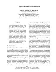
· 7acteristic, the communication bottleneck caps the potential for speeding up the algorithm.A study of high performance computing [Graham et al. 2005] shows that floating-pointinstructions historically improve at 59% per year, but inter-processor bandwidth improves26% per year, and inter-processor latency reduces only15% per year. The communicationbottleneck will only exacerbate over additional years.3.2 Strategies of PLDA+Let us first introduce pipeline-based Gibbs sampling. The pipeline technique has been usedin many applications to enhance throughput, such as the instruction pipeline in modernCPUs [Shen and Lipasti 2005] and in graphics processors [Blinn 1991]. Although pipelinedoes not decrease the time for a job to be processed, it can efficiently improve throughputby overlapping communication with computation. Fig. 4 illustrates the pipeline-basedGibbs sampling for four words, w 1 ,w 2 ,w 3 and w 4 . Fig. 4(A) demonstrates the case whent s ≥ t f +t u , and Fig. 4(B) the case whent s < t f +t u , wheret s ,t f andt u denote the timefor Gibbs sampling, fetching the topic distribution, and updating the topic distribution,respectively.In Fig. 4(A), PLDA+ begins by fetching the topic distribution for w 1 . Then it beginsGibbs sampling on w 1 , and at the same time, it fetches the topic distribution for w 2 . Afterit has finished Gibbs sampling forw 1 , PLDA+ updates the topic distribution forw 1 onP wprocessors. Whent s ≥ t f +t u , PLDA+ can begin Gibbs sampling onw 2 immediately afterit has completed sampling forw 1 . The total ideal time for PLDA+ to processW words willbe Wt s +t f +t u . Fig. 4(B) shows a suboptimal scenario where the communication timecannot be entirely masked. PLDA+ is not able to begin Gibbs sampling for w 3 until w 2has been updated and w 3 fetched. The example shows that in order to successfully maskcommunication, we must schedule tasks to ensure as much as possible that t s ≥ t f +t u .To make the pipeline strategy effective or t s ≥ t f + t u , PLDA+ divides processorsinto two types: one maintains documents and the document-topic count matrix to performGibbs sampling (P d processors), while the other stores and maintains the word-topic countmatrix (P w processors). The structure is shown in Fig. 2(B). During each iteration of Gibbssampling, aP d processor assigns a new topic to a word in a typical three-stage process:(1) Fetch the word’s topic distribution from aP w processor.(2) Perform Gibbs sampling and assign a new topic to the word.(3) Update theP w processors maintaining the word.The corresponding spread pattern for PLDA+ is illustrated in Fig. 3(C), which avoids boththe global synchronization of PLDA and the large number of iterations required by AS-LDA for convergence.One key property that PLDA+ takes advantage of is that each round of Gibbs samplingcan be performed in any word order. Since LDA models a document as a bag of words andignores word order, we can perform Gibbs sampling according to any word order as if wereordered words in bags. When a word that occurs multiple times in the documents of aP dprocessor, all instances of that word can be processed together. Moreover, for words thatoccur infrequently, we bundle them with words that occur more frequently to ensure thatt sis sufficiently long. In fact, if we knowt f +t u , we can decide how many word-occurrencesto process in each Gibbs sampling batch to ensure that t s −(t f +t u ) is minimized.To perform Gibbs sampling word by word, PLDA+ builds word indexes to documentson each P d processor. We then organize words in a circular queue as shown in Fig. 5.ACM Journal Name, Vol. V, No. N, Month 20YY.

8 ·TimeTimeWw 1FSUWw 1FSUw 2FSUw 2FSUw 3FSUw 3FSUw 4FSUw 4FSU(A)(B)Fig. 4: Pipeline-based Gibbs sampling in PLDA+. (A): t s ≥ t f + t u. (B): t s < t f + t u. In this figure, Findicates the fetching operation, U indicates the updating operation, and S indicates the Gibbs sampling operation.w 0w 1w 6w 7P d0P d1P d3w 5w 2w 4w 3P d2Fig. 5: Vocabulary circular queue in PLDA+.Gibbs sampling is performed by going around the circular queue. To avoid concurrentaccess to the same words, we schedule different processors to begin at different positionsof the queue. For example, Fig. 5 shows four P d processors, P d0 , P d1 , P d2 and P d3 starttheir first word from w 0 , w 2 , w 4 and w 6 , respectively. To ensure that this schedulingalgorithm works, PLDA+ must also distribute the word-topic matrix in a circular fashionon P w processors. This static allocation scheme enjoys two benefits. First, the workloadamong P w processors can be relatively balanced. Second, avoiding two P d nodes fromconcurrently updating the same word can roughly maintain serializability of the word-topicmatrix on P w nodes. Please note that the distributed scheme of PLDA+ ensures strongerserializability than PLDA because a P d node of PLDA+ can obtain the word-topic matrixupdates of other P d nodes in the same Gibbs sampling iteration. The detailed descriptionof word placement are presented in Section 3.3.1.Although word placement can be performed in an optimal way, scheduling must dealwith run-time dynamics. First, some processors may run faster than others, and this maybuild up bottlenecks at some of the P w processors. Second, when multiple requests arepending, the scheduler must be able to set priorities based on request deadlines. The detailsof PLDA+’s priority-based scheduling scheme are described in Section 3.4.3.3.3 Algorithm for P w ProcessorsThe task of the P w processors is to process, fetch and update queries from P d processors.PLDA+ distributes the word-topic matrix to P w processors according to the words containedin the matrix. After placement, each P w processor keeps approximately W/|P w |ACM Journal Name, Vol. V, No. N, Month 20YY.

10 ·(1) At the beginning, it allocates documents overP d processors and then builds an invertedindex for documents on each P d processor.(2) It groups the words in the vocabulary into bundles for performing Gibbs sampling andsending requests.(3) It schedules word bundles to minimize communication bottlenecks.(4) Finally, it performs pipeline-based Gibbs sampling iteratively until the terminationcondition is met.In the following, we present the four steps in detail.3.4.1 Document Allocation and Building an Inverted Index. Before performing Gibbssampling, we first have to distributeD documents toP d processors. The goal of documentallocation is to achieve good CPU load balance among P d processors. PLDA may sufferfrom imbalanced load since it has a global synchronization phase at the end of each Gibbssampling iteration, which may force fast processors to wait for the slowest processor. Incontrast, Gibbs sampling in PLDA+ is performed with no synchronization requirement. Inother words, a fast processor can start its next round of sampling without having to waitfor a slow processor. However, we also do not want some processors to be substantiallyslow and miss too many cycles of Gibbs sampling. This will result in the similar shortcomingthat AS-LDA suffers — taking a larger number of iterations to converge. Thus,we would like to allocate documents to processors in a balanced fashion. This is achievedby employing Random Document Allocation. EachP d processor gets approximateD/|P d |documents. The time complexity of this allocation step isO(D).After documents have been distributed, we build an inverted index for the documentsof each P d processor. Using this inverted index, each time a P d processor fetches thetopic distribution of a word w, it performs Gibbs sampling for all instances of w on thatprocessor. After sampling, the processor sends back the updated topic distribution to thecorresponding P w processor. The clear benefit is that for multiple occurrences of a wordon a processor, we only need to perform two communications, one fetch and one update,substantially reducing communication cost. The index structure for each wordw is:w → {(d 1 ,z 1 ),(d 1 ,z 2 ),(d 2 ,z 1 )...}, (4)in which, w occurs in document d 1 for 2 times and there are 2 entries. In implementation,to save memory, we will record all occurrences ofw ind 1 as one entry, (d 1 ,{z 1 ,z 2 }).3.4.2 Word bundle. Bundling words is to prevent the duration of Gibbs samplings frombeing too short to mask communication. Use an extreme example: a word takes place onlyonce on a processor. Performing Gibbs sampling on that word takes a much shorter timethan the time required to fetch and update the topic distribution of that word. The remedyis intuitive: combining a few words into a bundle so that the communication time can bemasked by the longer duration of Gibbs sampling time. The trick here is that we have tomake sure the target P w processor is the same for all words in a bundle so that each timeonly one communication IO is required for fetching topic distributions for all words in abundle.For a P d processor, we start bundling words according to their target P w processors.For all words with the same target P w processor, we first sort them in descending orderof occurrence times and build a word list. We then iteratively pick a high frequency wordfrom the head of the list and several low frequency words from the tail of the list and groupACM Journal Name, Vol. V, No. N, Month 20YY.

· 11them into a word bundle. After building word bundles, each time we will send a request tofetch topic distributions for all words in a bundle. For example, when learning topics fromNIPS dataset consisting of 12-year NIPS papers, we combine {curve, collapse, compiler,conjunctive,...} as a bundle, in which curve is a high frequency word and the rest are lowfrequency words in this dataset.3.4.3 Building the Request Scheduler. It is crucial to design an effective schedulerto determine the next word bundle to send requests for topic distributions during Gibbssampling. We employ a simple pseudo-random scheduling scheme.In this scheme, words in the vocabulary are stored in a circular queue. During Gibbssampling, words are selected from this queue in a clockwise or counterclockwise order.Each P d processor enters this circular queue with a different offset to avoid concurrentaccess to the same P w processor. The starting point of each P d process at each Gibbssampling iteration is different. This randomness avoids forming the same bottlenecks fromone iteration to another. Since circular scheduling is a static scheduling scheme, a bottleneckcan still be formed at some P w processors when multiple requests arrive at the sametime. Consequently, some P d processors may need to wait for a response before Gibbssampling can start. We remedy this shortcoming by registering a deadline for each request,as described in Section 3.3.2. Requests on aP w processor are processed according to theirdeadlines. A request will be discarded if its deadline has been missed. Due to the stochasticnature of Gibbs sampling, occasionally missing a round of Gibbs sampling does notaffect overall performance. Our pseudo-random scheduling policy ensures the probabilityof same words being skipped repeatedly is negligibly low.3.4.4 Pipeline-based Gibbs Sampling. Finally, we perform pipeline-based Gibbs sampling.As shown in Eq. (2), to compute and assign a new topic for a given wordx ij = w ina document d j , we have to obtain Cwword , C topic and Cj doc . The topic distribution of documentd j is maintained by a P d processor. While the up-to-date topic distribution Cwwordis maintained by a P w processor, the global topic count C topic should be collected overall P w processors. Therefore, before assigning a new topic for a word w in a document, aP d processor has to request Cwword and C topic from P w processors. After fetching CwwordandC topic , theP d processor computes and assigns new topics for occurrences of the wordw. Then the P d processor returns the updated topic distribution for the word w to theresponsible P w processor.For a P d processor pd, the pipeline scheme is performed according to the followingsteps:(1) Fetch overall topic counts for Gibbs sampling.(2) Select F word bundles and put them in the thread pool tp to fetch topic distributionsfor the words in each bundle. Once a request is responded by P w processors, thereturned topic distributions are put in a waiting queue Q pd .(3) For each word inQ pd , pick its topic distribution to perform Gibbs sampling.(4) After Gibbs sampling, put the updated topic distributions in the thread pooltp to sendupdate requests toP w processors.(5) Select a new word bundle and put it intp.(6) If the update condition is met, fetch new overall topic counts.ACM Journal Name, Vol. V, No. N, Month 20YY.

3.5 Parameters and Complexity· 13In this section, we analyze parameters that may influence the performance of PLDA+. Wealso analyze the complexity of PLDA+ and compare it with PLDA.3.5.1 Parameters. Given the total number of processors P , the first parameter is theproportion of the number ofP w processors toP d processors,γ = |P w |/|P d |. The larger thevalue ofγ, the more the average time for Gibbs sampling onP d processors will increase asfewer processors are used to perform CPU-bound tasks. At the same time, the average timefor communication will decrease since more processors serve as P w to process requests.We have to balance the number of P w and P d processors to (1) minimize both computationand communication time, and (2) ensure that communication time is short enoughto be masked by computation time. This parameter can be determined once we know theaverage time for Gibbs sampling and communication of the word-topic matrix. Supposethe total time for Gibbs sampling of the whole dataset is T s , the communication time fortransferring the topic distributions of all words from one processor to another processor isT t . For P d processors, the sampling time will beT s /|P d |. Suppose we transfer word topicdistributions simultaneously to P w processors, and thus transfer time will be T t /|P w |. Tomake sure the sampling process is able to overlap the fetching and updating process, wehave to make sureT s|P d | > 2T t|P w | . (5)Suppose T s = W¯t s where ¯t s is the average sampling time for all instances of a word, andT t = W¯t f = W¯t u , where ¯t f and ¯t u is the average fetching and update time for a word,we getγ = |P w||P d | > ¯t f +¯t u¯t s, (6)where ¯t f , ¯t u and ¯t s can be obtained by performing PLDA+ on a small dataset and thenempirically set an appropriate γ value. Under the computing environment for our experiments,we empirically set γ = 0.6.The second parameter is the number of threads in the thread pool R, which caps thenumber of parallel requests. Since the thread pool is used to prevent sampling from beingblocked by busy P w processors, R is determined by the network environment. R can beempirically tuned during Gibbs sampling. That is, when the waiting time for the prioriteration is long, the thread pool size is increased.The third parameter is the number of requests F for pre-fetching the topic distributionsbefore performing Gibbs sampling on P d processors. This parameter depends on R, andin experiments we set F = 2R.The last parameter is the maximum interval inter max for fetching the overall topiccounts from all P w processors during Gibbs sampling of P d processors. This parameterinfluences the quality of PLDA+. In experiments, we can achieve LDA models with similarquality to PLDA and LDA by settinginter max = W .It should be noted that the optimal values of the parameters of PLDA+ are highly relatedto the distributed environment, including network bandwidth and processor speed.3.5.2 Complexity. Table II summarizes the complexity of P d processors and P w processorsin both time and space. For comparison, we also list the complexity of LDA andACM Journal Name, Vol. V, No. N, Month 20YY.

14 ·Table II: Algorithm complexity. In this table,I is the iteration number of Gibbs sampling andcis a constant thatconverts bandwidth to flops.Method Time Complexity Space ComplexityPreprocessingGibbs samplingLDA - INK K(D +W)+NPLDAPLDA+,P dD|P|DWK+cW logW + |P d | |P w|I ( NKP+cKW logP)(N+KD)INK|P d |PLDA+,P w - -+KW P(N+KD)|P d |KW|P w|PLDA in this table. We assume P = |P w | + |P d | when comparing PLDA+ with PLDA.In this table, I indicates the iteration number for Gibbs sampling, and c is a constant thatconverts bandwidth to flops.The preprocessing of LDA distributes documents to P processors with time complexityD/|P|. Compared to PLDA, the preprocessing of PLDA+ requires three additionaloperations including (1) building an inverted document file for all documents on each P dprocessor with time O(D/|P d |), (2) bundling words with time O(W logW) for fast sortingwords according to their frequencies, and (3) sending topic counts from P d processorsto P w processors to initialize the word-topic matrix on P w with time O(WK/|P w |). Inpractice LDA is set to run with hundreds of iterations, and thus the preprocessing time forPLDA+ is insignificant compared to the training time.Finally, let us consider the speedup efficiency of PLDA+. Suppose γ = |P w |/|P d | forPLDA+, without considering preprocessing, the ideal achievable speedup is:speedup efficiency = S/PS/|P d | = |P d|P = 11+γ , (7)whereS denotes the running time for LDA on a single processor,S/P is the ideal time costusingP processors, andS/|P d | is the ideal time achieved by PLDA+ with communicationcompletely masked by Gibbs sampling.4. EXPERIMENTAL RESULTSWe compared the performance of PLDA+ with PLDA (AD-LDA based) through empiricalstudy. Our study focused on comparing both training quality and scalability. Since thespeedups of AS-LDA are just “competitive” to those reported for AD-LDA as shown in[Asuncion et al. 2008; 2010], we chose not to compare with AS-LDA.4.1 Datasets and Experiment EnvironmentWe used the three datasets shown in Table III. The NIPS dataset consists of scientificarticles from NIPS conferences. The NIPS dataset is relatively small, and we used it toinvestigate the influence of missed deadlines on training quality. Two Wikipedia datasetswere collected from English Wikipedia articles using the March 2008 snapshot from en.wikipedia.org. By setting the size of the vocabulary to 20,000 and 200,000, respectively,the two Wikipedia datasets are named Wiki-20T and Wiki-200T. Compared toWiki-20T, more infrequent words are added in vocabulary in Wiki-200T. However, evenfor those words ranked around 200,000, they have occurred in more than 24 articles inWikipedia, which is sufficient to learn and infer their topics using LDA. These two largeACM Journal Name, Vol. V, No. N, Month 20YY.

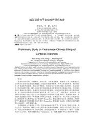
· 15Table III: Detailed information of data sets.NIPS Wiki-20T Wiki-200TD train 1,540 2,122,618 2,122,618W 11,909 20,000 200,000N 1,260,732 447,004,756 486,904,674D test 200 - -datasets were used for testing the scalability of PLDA+. In experiments, we implementedPLDA+ using a synchronous remote procedure call (RPC) mechanism. The experimentswere run on a distributed computing environment with2,048 processors, each with a2GHzCPU, 3GB of memory, and a disk allocation of 100GB.4.2 Impact of Missed DeadlinesSimilar to [Newman et al. 2007], we use test set perplexity to measure the quality of LDAmodels learned by various distributed methods of LDA. Perplexity is a common way ofevaluating language models in natural language processing, computed as:Perp(x test ) = exp ( − 1N test logp(xtest ) ) , (8)where x test denotes the test set, and N test is the size of the test set. A lower perplexityvalue indicates a better quality. For every test document in the test set, we randomlydesignated half the words for fold-in, and the remaining words were used for testing. Thedocument mixture θ j was learned using the fold-in part, and the log probability of thetest words was computed using this mixture. This arrangement ensures that the test wordswere not used in estimating model parameters. The perplexity computation follows thestandard method in [Griffiths and Steyvers 2004], which averages over multiple chainswhen making predictions using LDA models learned by Gibbs sampling. Using perplexityon the NIPS dataset, we find the quality and convergence rate of PLDA+ are comparableto single-processor LDA and PLDA. Since the conclusion is straightforward and similarto [Newman et al. 2007], we do not present the evaluation results on perplexity in detail.As described in Section 3.4.3, PLDA+ discards a request when its deadline is missed.Here we investigate the impact of missed deadlines on training quality using the NIPSdataset. We define missing ratio δ as the average number of missed requests divided bythe total number of requests, which ranges [0.0,1.0). By randomly dropping δ requestsin each iteration, we simulated discarding different amounts of requests in each iteration.We compared the quality of learned topic models under different δ values. In experimentswe set P = 50. Fig. 7 shows the perplexities with different δ values versus the numberof sampling iterations when K = 10. When the missing ratio is less than 60%, the perplexitiesremain reasonable. At interaction 400, the perplexities of δ’s between 20% and60% are about the same, whereas no deadline misses can achieve a 2% better perplexity.Qualitatively, a 2% perplexity drop does not show any discernible degradation in trainingresults. Fig. 8 shows the perplexities of converged topic models with various numbers oftopics versus different δ settings, at the end of iteration 400. A larger K setting suffersfrom more severe perplexity degradation. Nevertheless, δ = 60% seems to be a limitingthreshold that PLDA+ can endure. In reality, our experiments indicate that the missingratio is typically lower than 1%, far from the limiting threshold. Though the missing ratiodepends highly on the workload and the computation environment, the result of thisACM Journal Name, Vol. V, No. N, Month 20YY.

16 ·Perplexity280027002600250024002300ratio=0.0ratio=0.2ratio=0.4ratio=0.6ratio=0.8Perplexity220021002000190018002200210020000 100 200 300 400IterationFig. 7: Perplexity versus the number of iterationswhen missing ratio is 0.0, 0.2, 0.4, 0.6 and0.8.17001600K=10K=20K=800 0.1 0.2 0.3 0.4 0.5 0.6 0.7 0.8 0.9ratioFig. 8: Perplexity with various numbers of topics versusmissing ratio.experiment is encouraging that PLDA+ can operate well even when δ is high.4.3 Speedups and ScalabilityThe primary motivation for developing distributed algorithms for LDA is to achieve agood speedup. In this section, we report the speedup of PLDA+ compared to PLDA.We used Wiki-20T and Wiki-200T for speedup experiments. By setting the number oftopics K = 1,000, we ran PLDA+ and PLDA on Wiki-20T using P = 64,128,256,512and 1,024 processors, and on Wiki-200T using P = 64,128,256,512,1,024 and 2,048processors. Note that for PLDA+,P = P w +P d , and the ratio of|P w |/|P d | was empiricallyset toγ = 0.6 according to the unit sampling time and transfer time. The number of threadsin a thread pool was set asR = 50, which was determined based on the experiment results.1As analyzed in Section 3.5.2, the ideal speedup efficiency of PLDA+ is1+γ = 0.625.Fig. 9 compares speedup performance on Wiki-20T. The speedup was computed relativeto the time per iteration when using P = 64 processors, because it was impossible to runthe algorithms on a smaller number of processors due to memory limitations. We assumedthe speedup on P = 64 to be 64, and then extrapolated on that basis. From the figure, weobserve that whenP increases, PLDA+ simply achieves much better speedup than PLDA,thanks to the much reduced communication bottleneck of PLDA+. Fig. 10 compares theratio of communication time over computation time on Wiki-20T. When P = 1,024, thecommunication time of PLDA is13.38 seconds, which is about the same as its computationtime, much longer than that of PLDA+’s 3.68 seconds.From the results, we conclude that: (1) When the number of processors grows largeenough (e.g., P = 512), PLDA+ begins to achieve better speedup than PLDA; (2) In fact,if we take the waiting time for synchronization in PLDA into consideration, the speedupof PLDA could have been even worse. For example, in a busy distributed computingenvironment, when P = 128, PLDA may take about 70 seconds for communication inwhich only about10 seconds are used for transmitting word-topic matrices and most of thetime is used to wait for computation to complete.On the larger Wiki-200T dataset, as shown in Fig. 11, the speedup of PLDA starts toflatten out at P = 512, whereas PLDA+ continues to gain in speed 1 . For this dataset,1 For PLDA+, the parameter of pre-fetch number and thread pool size was set to F = 100 and R = 50. WithW = 200,000 and K = 1,000, the matrix is 1.6GBytes, which is large for communication.ACM Journal Name, Vol. V, No. N, Month 20YY.

· 17Speedups1000900800700600500400300200PerfectPLDAPLDA+Time for One Iteration (Seconds)30025020015010050CommunicationSampling100200 400 600 800 1000Number of Processors064 128 256 512 1024Number of Processors (Left: PLDA, Right: PLDA+)Fig. 9: Parallel speedup results for 64 to 1,024 processorson Wiki-20T.Fig. 10: Communication and sampling time for 64 to1,024 processors on Wiki-20T.Speedups200018001600140012001000800600400200PerfectPLDAPLDA+500 1000 1500 2000Number of ProcessorsTime for One Iteration (Seconds)350300250200150100500CommunicationSampling64 128 256 512 1024 2048Number of Processors (Left: PLDA, Right: PLDA+)Fig. 11: Parallel speedup results for 64 to 2,048 processorson Wiki-200T.Fig. 12: Communication and sampling time for 64 to2,048 processors on Wiki-200T.we also list the sampling and communication time ratio of PLDA and PLDA+ in Fig. 12.PLDA+ keeps the communication time to consistently low values from P = 64 to P =2,048. When P = 2,048, PLDA+ took only about 20 minutes to finish 100 iterationswhile PLDA took about 160 minutes. Though eventually Amdahl’s Law would kick in tocap speedup, it is evident that the reduced overhead of PLDA+ permits it to achieve muchbetter speedup for training on large-scale datasets using more processors.The above comparison did not take preprocessing into consideration because the preprocessingtime of PLDA+ is insignificant compared to the training time as analyzed in Section3.5.2. For example, the preprocessing time for the experiment setting of P = 2,048on Wiki-200T is 35 seconds. For training, hundreds of iterations are required, with eachiteration taking about 13 seconds.5. CONCLUSIONIn this paper, we presented PLDA+, which employs data placement, pipeline processing,word bundling, and priority-based scheduling strategies to substantially reduce intercomputercommunication time. Extensive experiments on large-scale datasets demonstratedthat PLDA+ can achieve much better speedup than previous attempts on a distributedenvironment.ACM Journal Name, Vol. V, No. N, Month 20YY.

18 ·AcknowledgmentsWe thank the anonymous reviewers for their insightful comments. We also thank MattStanton, Hongjie Bai, Wen-Yen Chen and Yi Wang for their pioneering work, and thankXiance Si, Hongji Bao, Tom Chao Zhou, Zhiyu Wang for helpful discussions. This workis supported by Google-Tsinghua joint research grant.REFERENCESASUNCION, A., SMYTH, P., AND WELLING, M. 2008. Asynchronous distributed learning of topic models. InProceedings of NIPS. 81–88.ASUNCION, A., SMYTH, P., AND WELLING, M. 2010. Asynchronous distributed estimation of topic modelsfor document analysis. Statistical Methodology.BERENBRINK, P., FRIEDETZKY, T., HU, Z., AND MARTIN, R. 2008. On weighted balls-into-bins games.Theoretical Computer Science 409, 3, 511–520.BLEI, D. M., NG, A. Y., AND JORDAN, M. I. 2003. Latent dirichlet allocation. Journal of Machine LearningResearch 3, 993–1022.BLINN, J. 1991. A trip down the graphics pipeline: Line clipping. IEEE Computer Graphics and Applications11, 1, 98–105.CHEMUDUGUNTA, C., SMYTH, P., AND STEYVERS, M. 2007. Modeling general and specific aspects of documentswith a probabilistic topic model. In Proceedings of NIPS. 241–248.CHEN, W., CHU, J., LUAN, J., BAI, H., WANG, Y., AND CHANG, E. 2009. Collaborative filtering for orkutcommunities: discovery of user latent behavior. In Proceedings of WWW. 681–690.CHU, C.-T., KIM, S. K., LIN, Y.-A., YU, Y., BRADSKI, G., NG, A. Y., AND OLUKOTUN, K. 2006. Mapreducefor machine learning on multicore. In Proceedings of NIPS.DEAN, J. AND GHEMAWAT, S. 2004. Mapreduce: Simplified data processing on large clusters. In Proceedingsof OSDI. 137–150.GOMES, R., WELLING, M., AND PERONA, P. 2008. Memory bounded inference in topic models. In Proceedingsof ICML. 344–351.GRAHAM, S., SNIR, M., AND PATTERSON, C. 2005. Getting up to speed: The future of supercomputing.National Academies Press.GRIFFITHS, T. AND STEYVERS, M. 2004. Finding scientific topics. Proceedings of the National Academy ofSciences of the United States of America 101, 90001, 5228–5235.LI, W. AND MCCALLUM, A. 2006. Pachinko allocation: DAG-structured mixture models of topic correlations.In Proceedings of ICML.MIMNO, D. M. AND MCCALLUM, A. 2007. Organizing the OCA: learning faceted subjects from a library ofdigital books. In Proceedings of ACM/IEEE Joint Conference on Digital Libraries. 376–385.NEWMAN, D., ASUNCION, A., SMYTH, P., AND WELLING, M. 2007. Distributed inference for latent dirichletallocation. In Proceedings of NIPS. 1081–1088.NEWMAN, D., ASUNCION, A., SMYTH, P., AND WELLING, M. 2009. Distributed algorithms for topic models.Journal of Machine Learning Research 10, 1801–1828.PORTEOUS, I., NEWMAN, D., IHLER, A., ASUNCION, A., SMYTH, P., AND WELLING, M. 2008. Fast collapsedgibbs sampling for latent dirichlet allocation. In Proceedings of KDD. 569–577.ROSEN-ZVI, M., CHEMUDUGUNTA, C., GRIFFITHS, T., SMYTH, P., AND STEYVERS, M. 2010. Learningauthor-topic models from text corpora. ACM Transactions on Information Systems 28, 1, 1–38.SHEN, J. P. AND LIPASTI, M. H. 2005. Modern Processor Design: Fundamentals of Superscalar Processors.McGraw-Hill Higher Education.WANG, Y., BAI, H., STANTON, M., CHEN, W., AND CHANG, E. 2009. PLDA: Parallel latent dirichlet allocationfor large-scale applications. In Algorithmic Aspects in Information and Management. 301–314.YAN, F., XU, N., AND QI, Y. 2009. Parallel inference for latent dirichlet allocation on graphics processing units.In Proceedings of NIPS. 2134–2142.ACM Journal Name, Vol. V, No. N, Month 20YY.