Mathematics for Management Science Notes 05

Mathematics for Management Science Notes 05
prepared by Professor Jenny Baglivo
© Jenny A. Baglivo 2002. All rights reserved.
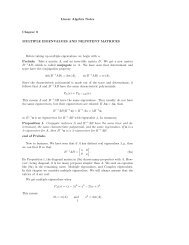
Transportation and assignment problems
Transportation/assignment problems arise frequently in planning for the distribution of
goods and services from several supply locations (origins) to several demand locations
(destinations). Transportation/assignment is to be made at minimum cost.
Origins are indexed using i=1, 2, etc. Destinations are indexed using j=1, 2, etc. Typical
notation is as follows:
• For the decision variables, we let x ij equal the number of units shipped from origin i
to destination j.
• The supply at origin i is denoted by s i .
• The demand at destination j is denoted by d j .
If the total supply is greater than or equal to the total demand, then
• For each origin, the constraint x i+ ≤ s i is added to the model and
• For each destination, the constraint x +j = d j is added to the model.
(Not all products are shipped. All demands are satisfied.)
If the total supply is less than the total demand, then
• For each origin, the constraint x i+ = s i is added to the model and
• For each destination, the constraint x +j ≤ d j is added to the model.
(All products are shipped. Not all demands are satisfied.)
page 1 of 19

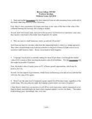
Exercise 1:
Tropicsun is a leading grower and distributor of fresh citrus products with three large
citrus groves scattered around central Florida in the cities of Mt. Dora, Eustis, and
Clermont. Tropicsun currently has 275,000 bushels of citrus at the grove in Mt. Dora,
400,000 bushels at the grove in Eustis, and 300,000 at the grove in Clermont.
Tropicsun has citrus processing plants in Ocala, Orlando, and Lessburg with processing
capacities to handle 200,000, 600,000, and 225,000 bushels, respectively. Tropicsun
contracts with a local trucking company to transport its fruit from the groves to the
processing plants. The trucking company charges a flat rate for every mile that each
bushel of fruit must be transported. Each mile a bushel of fruit travels is known as a
bushel-mile. The following table summarizes the distances (in miles) between the groves
and processing plants:
to Ocala to Orlando to Leesburg
from Mt. Dora 21 50 40
from Eustis 35 30 22
from Clermont 55 20 25
Tropicsun wants to determine how many bushels to ship from each grove to each
processing plant in order to minimize the total number of bushel-miles.
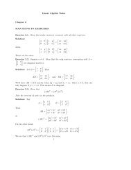
Note: The problem can be visualized using a transportation network, where each source and
destination is represented as a node, and each route from source to destination as a link.
Mt Dora
page 2 of 19
Ocala
Eustis Orlando
Clermont
Leesburg

• Define the decision variables precisely
• Completely specify the LP model
page 3 of 19

• Clearly state the optimal solution.
• How would the total cost change if Leesburg could only process 200,000 bushels?
• Interpret the reduced cost for shipping from Eustis to Ocala.
page 4 of 19

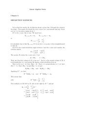
Exercise 1 solution sheet:
1
2
3
4
5
6
7
8
9
10
11
12
13
14
15
16
17
18
19
20
21
22
23
24
25
26
27
28
29
30
31
32
33
34
35
36
37
A B C D E F G H
Tropicsun
Distance (miles)
to Ocala to Orlando to Leesburg Supply:
from Mt. Dora 21 50 40 275000
from Eustis 35 30 22 400000
from Clermont 55 20 25 300000
M O D E L
Capacity: 200000 600000 225000
Minimize Total
B u s h e l - M i l e s 24000000
Decision Variables
to Ocala to Orlando to Leesburg L H S R H S
from Mt. Dora 200000 0 75000 275000 = 275000
from Eustis 0 250000 150000 400000 = 400000
from Clermont 0 300000 0 300000 = 300000
L H S 200000 550000 225000

Sensitivity and formulas sheets:
Adjustable Cells
F i n a l Reduced O b j e c t i v e A l l o w a b l e A l l o w a b l e
C e l l N a m e V a l u e C o s t C o e f f i c i e n t I n c r e a s e D e c r e a s e
$B$18 from Mt. Dora to Ocala 200000 0 21 27 1E+30
$C$18 from Mt. Dora to Orlando 0 2 50 1E+30 2
$D$18 from Mt. Dora to Leesburg 75000 0 40 2 27
$B$19 from Eustis to Ocala 0 32 35 1E+30 32
$C$19 from Eustis to Orlando 250000 0 30 2 8
$D$19 from Eustis to Leesburg 150000 0 22 8 2
$B$20 from Clermont to Ocala 0 62 55 1E+30 62
$C$20 from Clermont to Orlando 300000 0 20 13 1E+30
$D$20 from Clermont to Leesburg 0 13 25 1E+30 13
Constraints
1
2
3
4
5
6
7
8
9
10
11
12
13
14
15
16
17
18
19
20
21
22
23
24
F i n a l S h a d o w C o n s t r a i n t A l l o w a b l e A l l o w a b l e
C e l l N a m e V a l u e P r i c e R.H. Side I n c r e a s e D e c r e a s e
$F$18 from Mt. Dora LHS 275000 48 275000 50000 75000
$F$19 from Eustis LHS 400000 30 400000 50000 250000
$F$20 from Clermont LHS 300000 20 300000 50000 300000
$B$22 LHS to Ocala 200000 -27 200000 75000 50000
$C$22 LHS to Orlando 550000 0 600000 1E+30 50000
$D$22 LHS to Leesburg 225000 - 8 225000 250000 50000
A B C D E F G H
T r o p i c s u n
to Ocala
Distance (miles)
to Orlando to Leesburg Supply:
from Mt. Dora 21 50 40 275000
from Eustis 35 30 22 400000
from Clermont 55 20 25 300000
M O D E L
Capacity: 200000 600000 225000
Minimize Total
B u s h e l - M i l e s =SUMPRODUCT(B5:D7,B18:D20)
Decision Variables
to Ocala to Orlando to Leesburg L H S R H S
from Mt. Dora 0 0 0 =SUM(B18:D18) = =F5
from Eustis 0 0 0 =SUM(B19:D19) = =F6
from Clermont 0 0 0 =SUM(B20:D20) = =F7
L H S =SUM(B18:B20) =SUM(C18:C20) =SUM(D18:D20)

Assignment problems are special cases of transportation problems where s i = d j = 1.
Exercise 2:
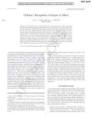
Fowle Marketing Research Company has just received requests for market research
studies from three new clients. The company faces the task of assigning a project leader
to each client. Currently, four individuals have no other commitments and are available
for the project leader assignments. Fowle’s management realizes, however, that the time
required to complete each study will depend on the experience and ability of the project
leader assigned. Estimated project completion times in days are given in the following
table:
Project Leader: Client 1 Client 2 Client 3
1: Terry 10 15 9
2: Carle 9 18 5
3: McClymonds 6 14 3
4: Higley 8 16 6
The three projects have approximately the same priority, and the company wants to
assign project leaders to minimize the total number of days required to complete all three
projects. If a project leader is to be assigned to one client only, what assignments should
be made?
This problem could be solved by enumerating all 24 possible assignments of three of the
four project leaders to the clients.
page 7 of 19

• Define the decision variables precisely
• Completely specify the LP model
• Clearly state the optimal solution
page 8 of 19

Solution and sensitivity sheets:
1
2
3
4
5
6
7
8
9
10
11
12
13
14
15
16
17
18
19
20
21
22
23
24
25
A B C D E F G H
Fowle Marketing
Completion Time (days)
to Client 1 to Client 2 to Client 3
Terry assigned 10 15 9
Carle assigned 9 18 5
McClymonds assigned 6 14 3
Higley assigned 8 16 6
M O D E L
Minimize Total
Completion Time: 26
Decision Variables
to Client 1 to Client 2 to Client 3 L H S R H S
Terry assigned 0 1 0 1

Transshipment problems:
Transshipment problems have the same basic goals as transportation problems (in
particular, there is a need to ship goods from origins to destinations at minimum cost),
but
• Goods may travel from a source through an intermediate location (known as a
transshipment node) to a destination,
• Some destinations may also serve as transshipment points to other destinations,
• etcetera.
The locations (sources, destinations, and transshipment points) are visualized as nodes in
a network, and are numbered consecutively. If nodes i and j are connected by a direct
route in the network (a link), then the decision variable x ij is used to represent the number
of items shipped from node i to node j. For example, if a company has
1. two plants (sources),
2. a warehouse (serving as a pure transshipment point), and
3. two retail outlets (destinations),
a transportation network could look like the following:
1: Plant 1 4: Outlet 1
2: Plant 2 5: Outlet 2
3: Warehouse
The links correspond to (i, j) equal to (1,3), (1,4), (1,5), (2,3), (2,4), (2,5), (3,4), (3,5).
page 10 of 19

For each node in the network, there is a flow constraint, where the left and right hand
sides are as follows:
(1) LHS = OUTFLOW – INFLOW
(2) RHS = supply with a plus sign or demand with a negative sign or zero if it is a
pure transshipment node.
The outflow corresponds to the number of units leaving a given node. The inflow
corresponds to the number of units entering a given node.
You can use the same relational symbol ( = , ≤ , ≥ ) for all flow constraints:
Total Supply = Total Demand LHS = RHS
Total Supply > Total Demand LHS ≤ RHS
Total Supply < Total Demand LHS ≥ RHS
Exercise 3:
A company has two plants (at nodes 1 and 2), one regional warehouse (at node 3), and
two retail outlets (at nodes 4 and 5). In the next production cycle:
1. Plants 1 and 2 can produce 400 and 600 units of product, respectively,
2. Outlets 1 and 2 have a demand for 750 and 250 units of product, respectively, and
3. The costs for shipping each unit of the product are as follows:
From1 to 3 $4 From 2 to 4 $9
From 1 to 4 $10 From 2 to 5 $6
From 1 to 5 $8 From 3 to 4 $2
From 2 to 3 $4 From 3 to 5 $3
At most 500 units can be shipped between the warehouse and the outlet at node 4.
The company wants to determine the least costly way to ship the units.
page 11 of 19

• Construct the transshipment network, including supplies and demands (with appropriate signs),
and costs along each route.
• Define the decision variables precisely
• Completely specify the LP model
page 12 of 19

• Clearly state the optimal solution
• Interpret the shadow price and range of feasibility for the last constraint.
page 13 of 19

Exercise 3 solution sheet:
1
2
3
4
5
6
7
8
9
10
11
12
13
14
15
16
17
18
19
20
21
22
23
24
25
26
27
28
29
30
31
32
33
34
35
36
37
38
39
40
41
42
43
44
45
A B C D E F
Company with
W a r e h o u s e
Supply(+)/
Nodes: Demand(-)
1: Plant 1 400 Warehouse Max
2: Plant 2 600 to Outlet 1: 500
3: Whs 0
4: Outlet 1 -750
5: Outlet 2 -250
D e c i s i o n
V a r i a b l e s :
Unit Cost #Units
1 to 3 4 400
1 to 4 10 0
1 to 5 8 0
2 to 3 4 100
2 to 4 9 250
2 to 5 6 250
3 to 4 2 500
3 to 5 3 0
M i n i m i z e
Total Cost: 6750
Subject to
Outflow Inflow L H S R H S
Node 1 flow 400 400 = 400
Node 2 flow 600 600 = 600
Node 3 flow 500 500 0 = 0
Node 4 flow 750 -750 = -750
Node 5 flow 250 -250 = -250
Whs to Outlet 1 500

Sensitivity and formulas sheets:
Adjustable Cells
F i n a l Reduced O b j e c t i v e A l l o w a b l e A l l o w a b l e
C e l l N a m e V a l u e C o s t C o e f f i c i e n t I n c r e a s e D e c r e a s e
$D$14 1 to 3 #Units 400 0 4 1 1E+30
$D$15 1 to 4 #Units 0 1 10 1E+30 1
$D$16 1 to 5 #Units 0 2 8 1E+30 2
$D$17 2 to 3 #Units 100 0 4 3 1
$D$18 2 to 4 #Units 250 0 9 1 3
$D$19 2 to 5 #Units 250 0 6 1 1E+30
$D$20 3 to 4 #Units 500 0 2 3 1E+30
$D$21 3 to 5 #Units 0 1 3 1E+30 1
Constraints
F i n a l S h a d o w C o n s t r a i n t A l l o w a b l e A l l o w a b l e
C e l l N a m e V a l u e P r i c e R.H. Side I n c r e a s e D e c r e a s e
$D$28 Node 1 flow LHS 400 0 400 100 0
$D$29 Node 2 flow LHS 600 0 600 0 1E+30
$D$30 Node 3 flow LHS 0 - 4 0 100 0
$D$31 Node 4 flow LHS -750 - 9 -750 250 0
$D$32 Node 5 flow LHS -250 - 6 -250 250 0
$D$34 Whs to Outlet 1 LHS 500 - 3 500 0 100
1
2
3
4
5
6
7
8
9
10
11
12
13
14
15
16
17
18
19
20
21
22
23
24
25
26
27
28
29
30
31
32
33
34
A B C D E F
Company with
W a r e h o u s e
Supply(+)/
Nodes: Demand(-)
1: Plant 1 400 Warehouse Max
2: Plant 2 600 to Outlet 1: 500
3: Whs 0
4: Outlet 1 -750
5: Outlet 2 -250
D e c i s i o n
V a r i a b l e s :
Unit Cost #Units
1 to 3 4 400
1 to 4 10 0
1 to 5 8 0
2 to 3 4 100
2 to 4 9 250
2 to 5 6 250
3 to 4 2 500
3 to 5 3 0
M i n i m i z e
Total Cost: =SUMPRODUCT(B14:B21,D14:D21)
Subject to
Outflow Inflow L H S R H S
Node 1 flow =SUM(D14:D16) =B28-C28 = =B5
Node 2 flow =SUM(D17:D19) =B29-C29 = =B6
Node 3 flow =SUM(D20:D21) =D14+D17 =B30-C30 = =B7
Node 4 flow =D15+D18+D20 =B31-C31 = =B8
Node 5 flow =D16+D19+D21 =B32-C32 = =B9
Whs to Outlet 1 =D20

Exercise 4:
The Bavarian Motor Company (BMC) manufactures expensive luxury cars in Hamburg,
Germany, and exports cars to sell in the United States. The exported cars are shipped from
Hamburg to ports in Newark, New Jersey, and Jacksonville, Florida. From these ports, the
cars are transported by rail or truck to distributors located in Boston, Columbus, Atlanta,
Richmond, and Mobile.
1. There are 200 cars in Newark and 300 in Jacksonville.
2. The numbers of cars needed in Boston, Columbus, Richmond, Atlanta, and Mobile are
100, 60, 80, 170, and 70, respectively.
3. Per car shipping costs are as follows (see the graph for numbering):
From 1 to 2 $30 From 5 to 6 $35
From 1 to 4 $40 From 6 to 5 $25
From 2 to 3 $50 From 7 to 4 $50
From 3 to 5 $35 From 7 to 5 $45
From 5 to 3 $40 From 7 to 6 $50
From 5 to 4 $30
BMC would like to determine the least costly way of transporting the cars from the ports
to the locations where they are needed.
• Complete the following transshipment network by filling in the supplies and demands (with
appropriate signs) and the unit costs along each link.
2: Boston
3: Columbus 1: Newark
5: Atlanta 4: Richmond
6: Mobile 7: Jacksonville
page 16 of 19

• Define the decision variables precisely
• Completely specify the LP model
page 17 of 19

• Clearly state the optimal solution.
• Interpret the shadow price of the first constraint, and its range of feasibility.
page 18 of 19

Exercise 4 solution and sensitivity reports:
1
2
3
4
5
6
7
8
9
10
11
12
13
14
15
16
17
18
19
20
21
22
23
24
25
26
27
28
A B C D E F
Bavarian
Motor Works
Supply(+)/ Decision
Demand(-) V a r i a b l e s :
City 1 200 Unit Cost: #Cars
City 2 -100 1 to 2 30 120
City 3 -60 1 to 4 40 80
City 4 -80 2 to 3 50 20
City 5 -170 3 to 5 35 0
City 6 -70 5 to 3 40 40
City 7 300 5 to 4 30 0
5 to 6 35 0
6 to 5 25 0
7 to 4 50 0
7 to 5 45 210
7 to 6 50 70
M i n i m i z e
Total Cost: 22350
Subject to
Outflow Inflow L H S R H S
City 1 flow 200 200