Summary - IPPCR Video and Handout Archive

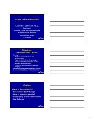
Objectives• Review part of course content• Compare randomized experimental studiesto nonrandomzied and observational studies• Prepare for remainder of the course

Outline‣Exam information• Take home messages and exercisesfrom several (but not all) of the lectures• Answering questions from thediscussion boards• More information on OR, RR, andlogistic regression• Conclusions and questions

Exam• Students will only have one opportunity totake the exam• Participants scoring 75% or higher will beawarded a certificate of successfulcompletion• Certificates t can be printed from the coursewebsite using your log-in information

Preparation & PracticeQuestions• Consider rewatching the videos• 3 rd edition of course text book– Practice questions and exercises at end ofeach chapter– Some are more detailed than others• Exam questions/answers from lecturers– Chapter not always written by lecturer• My questions are usually like questions atend of 3 rd Ed Chapters 18, 19, 23, maybe 21– Not the questions in the text book

OutlineExam information‣Take home messages and exercisesfrom several (but not all) of the lectures• Answering questions from thediscussion boards• More information on OR, RR, andlogistic regression• Conclusions and questions

Study Design

Intervention Based ResearchSpectrum• Epidemiology• Quasi-experimental• Pre-clinical studies• Phase 0• Phase I• Early/Late Phase II• Phase III• Phase IV• Dissemination and Implementation• Comparative or Cost EffectivenessPPCR 201210

Study Design Taxonomy• Intervention vs. Observational• Longitudinal vs. Cross-sectional• Prospective vs. Retrospective• Blinded/Masked or Not Blinded/Masked– Single-blind, Double blind, Unblinded• Randomized d vs. Non-RandomizeddPPCR 201211

Types of Randomized Studies• Parallel Group – classic• Sequential Trials – physical sciences• Group Sequential trials – classic• Cross-over – intervention washout• Factorial Designs – independence• Adaptive Designs – gaining i popularity• Enriched Enrollment – regression to themean• Cluster Randomized DesignsPPCR 2012 12

Observational Studies• Case Reports• Case Series• Cross-Sectional or Prevalence Surveys• Case-Control Study• Cohort Study (longitudinal)• Natural History StudiesPPCR 2012 13

Epidemiology• Study of the distribution and determinantsof disease and injury in human, animal,plant, or other populations– [Human] disease does not occur atrandom– [Human] disease has causal andpreventive factors that can be identifiedthrough systematic investigation ofdifferent populations or subgroups ofindividuals within a populationp• Hennekens and Buring, 1987

Observational Studies• Case Reports/Case Series• Cross-sectional Survey– NHIS (National Health Interview Survey)• Case-Control Control Study– Groups with or without outcome– Determine who was exposed to risk factor• Cohort Study– Follow a group for a while– Cardiovascular Health Study

Non-Randomized• Can ONLY showAssociation• You will neverknow all possibleconfounders!Randomized• Can showAssociation ANDCausality• Well done nonadaptiverandomization →unknownconfounders shouldnot create problemsPPCR 201216

Randomization

Random Example (Game 1)• Everybody get a coin– Designate one side “Heads” and theopposite side “Tails”• Flip the coin• How many heads (raise hands)• How are the heads clustered (vs tails)clustered together?18

Random Example (Game 2)• Everybody pick a random number from thislist0 1 2 3 4 5 6 7 8 9 1019

Motivation Behind Randomization• Provides basis for valid statistical testsbetween treatment groups• Randomization means we can attributecausality, i.e. any between group differencein outcomes can be attributed to thetreatment– In truth, randomization does not guaranteecausality is the ‘difference’, but itincreases the likelihood that causality isthe main driving factor20

Features of Randomization• Random Allocation– Known chance receiving a treatment– Cannot predict the treatment t t to be given– Scheme is reproducible• Reduces selection bias when allocating tostudy arms• Similar treatment groups– Patient characteristics will tend to bebalanced across study arms– Chance baseline imbalances betweengroups may still occur21

Randomization Summary• Permuted block randomization often the best– Stratify on only a few factors and perhapsnot at all– Choose block size(s) appropriate tosample size• Randomize smallest independent d element atlast possible second• Proper documentation as important asproper implementation22

Randomization Summary• Masking/blinding is key for preventing biasMasking/blinding is key for preventing bias• ITT (intent to treat) analysis necessary topreserve randomization and infer causality,or lack thereof

Intent to Treat vs. Completers• ITT = Intent To Treat analysis– Assume all study participants• Adhered to the study regime assigned• Completed the study– Only analysis to preserve randomization• MITT = Modified ITT analysis– ITT, but only include people who take thefirst dosage• Per Protocol-Completers-Adherers analysis– Only the well behaved

Simple Important Steps to Avoid Problems• Check eligibility criteria thoroughly prior toenrollment– Unnecessary drop out if realize afterrandomization subject not eligible andforced to withdraw– No matter how quickly a subject iswithdrawn all randomized subjects includedin ITT• Avoid a delay between randomization andtreatment initiation– Delays can lead to unnecessary missingdata that affects ITT25

Ways to Randomize• Standard ways:– Random number tables (see text)– Computer programs– randomization.com• Three randomization plan generators• NOT legitimatet– Birth date– Last digit of the medical record number– Odd/even room number

Who/What to Randomize - Independence• Person– Common unit of randomization in RCTs– Might take several biopsies/person• Provider– Doctor– Nursing station• Locality– School– Community• Sample size is predominantly determined bythe number of randomized units

Types of Randomization• Simple• Blocked Randomization• Stratified Randomization• Baseline Covariate AdaptiveRandomization/Allocation• Response Adaptive Randomization orAllocation (using interim data)• Cluster Randomization

Hypothesis Testing

Statistical Inference• Inferences about a population are made onthe basis of results obtained from a sampledrawn from that population• Want to talk about the larger population fromwhich the subjects are drawn, not theparticular subjects!

Take Home: Hypothesis Testing• Many ways to test– Rejection interval– Z test, t test, or Critical Value– P-value– Confidence interval• For this, all ways will agree– If not: math wrong, rounding errors• Make sure interpret correctly

Take Home Hypothesis Testing• How to turn questions into hypotheses• Failing to reject the null hypothesisDOES NOT mean that the null is true• Every test has assumptions– A statistician can check all theassumptions– If the data does not meet the assumptionsthere are non-parametric versions of tests(see text)

Never “Accept” Anything• Reject the null hypothesis• Fail to reject the null hypothesis• Failing to reject the null hypothesis doesNOT mean the null (H 0 ) is true• Failing to reject the null means– Not enough evidence in your sample toreject the null hypothesis– In one sample saw what you saw

Tak e Home:V ocabulary• Null Hypothesis: H 0• Alternative Hypothesis: H 1 or H a or H A• Significance Level: α level• Acceptance/Rejection Region• Statistically Significant• Test Statisticti ti• Critical Value• P-value, Confidence Interval

Little Diagnostic TestingLingo• False Positive/False Negative (α, β)• Positive Predictive Value (PPV)– Probability diseased given POSITIVEtest result• Negative Predictive Value (NPV)– Probability bilit NOT diseased d givenNEGATIVE test result• Predictive values depend on diseaseprevalence

High ORDoes Not a Good Test Make• Diagnostic tests need separationDiagnostic tests need separation• ROC curves– Not logistic regression with high OR• Strong association between 2 variables doesnot mean good prediction of separation

Avoid Common Mistakes:Hypothesis Testing• Mistake: assume independent measurements• Tests have assumptions of independence– Taking multiple samples per subject ?Statistician MUST know– Different statistical analyses MUST beused and they can be difficult!• Mistake: ignore distribution of observations– Histogram of the observations– Highly skewed data - t test and even nonparametrictests can have incorrect results

Estimates and P-V PV alues• Group A: 25±9Group A: 25±9• Group B: 10±9• 25 vs. 10 wow a big difference!– Um, no. 15±12.7– Calculate the 95% CIs

Comparing A to B• Appropriatep– Statistical properties of A-B– Statistical properties of A/B• NOT Appropriate– Statistical properties of A– Statistical properties p of B– Look they are different!

Sample Size and Power

Tak e Away Message• Get some input from a statistician– This part of the design is vital andmistakes can be costly!• Take all calculations with a few grainsof salt– “Fudge factor” is important!• Round UP, never down (ceiling)– Up means 10.01 becomes 11• Analysis Follows Design

Tak eAway• Study’s primary outcome– Basis for sample size calculation– Secondary outcome variables consideredimportant? Make sure sample size issufficient• Increase the ‘real’ sample size to reflect lossto follow up, expected response rate, lack ofcompliance, etc.– Make the link between the calculation andincrease• Always round up– Sample size = 10.01; need 11 people

Take Home: What you need for N• What difference is scientifically important inunits – thought, disc.– 0.01 inches?– 10 mm Hg in systolic BP?• How variable are the measurements(accuracy)? – Pilot!– Plastic ruler, Micrometer, Caliper

Tak e Home: N• Difference (effect) to be detected (δ)• Variation in the outcome (σ 2 )• Significance level (α)– One-tailed vs. two-tailed tests• Power• Equal/unequal arms• Superiority or equivalence or noninferiority• Variables of interest

Basic Sample Size• Changes in the difference of interest haveHUGE impacts on sample size– 20 point difference → 25 patients/group– 10 point difference → 100 patients/groupp– 5 point difference → 400 patients/group• Changes in difference to be detected, α, β, σ,number of samples, if it is a 1- or 2-sided testcan all have a large impact on your samplesize calculationBasic 2-Arm Study’sTOTAL Sample Size = 2N24( Z )2 21 /2 Z1 2

If I cut my difference of interestin half?• I increase my sample size FOUR foldI increase my sample size FOUR fold• All other things equal

Concepts of Time to Event Analysis

Define the OutcomeV ariable• What is the event? (Death?)• Where is the time origin? (Diagnosis?)• What is the time scale? (Weeks? Years?)• Then what?– Need to know the time the event occurs– May or may not use covariates57

Bottom Line• Survival analysis deals with makinginference about EVENT RATES• Rate at t = Rate among those at risk at t• Standard d methods to deal with rightcensoring and left truncation• Key assumption is that those at risk at t are arandom sample from the population ofinterest at risk at t• Independent censoring58

Kaplan Meier• One way to estimate survival• Nice, simple, can compute by hand• Can add stratification factors• Cannot evaluate covariates like Cox model• No sensible interpretation for competingrisks59

Inference: Log Rank• Logrank statistics compare event rates andallow the same generality as right censoring,left truncation• For single event data inference about rates→ inference for S(t)– No time dependent d covariates, norecurrent events, no competing risk events– May be misleading60

Cox Model for Event Rates• Provides a framework for making inferenceabout covariate effects• Requires either that– RR is constant over time (proportionalhazards), or– That we model RR over time• Allows time-dependent covariates andstratification factors61

OutlineExam informationTake home messages and exercisesfrom several (but not all) of the lectures‣Answering questions from thediscussion boards• More information on OR, RR, andlogistic regression• Conclusions and questions

Prevalence vs. Incidence• “In the slides: "#with disease/# at risk”In the slides: #with disease/# at risk– I am confused about the # at risk• Is # all population?• Is over people at risk the same asincidence?”

Cohort Study Question• “Why in a prospective cohort study rareWhy in a prospective cohort study raredisease cannot be studied but rare exposurecan be studied?”

Effect Modification Link NEW• http://www.sld.cu/galerias/pdf/sitios/vigilancia/asite2_chapter_7.pdf

Enrichment Study Designs• ‘When can we use these designs and how dothey relate to regression to the mean?’• Design choice depends on study question• Regression to the mean in this situationconcerns if enrolling ‘right’ people– During run-in phase potential participantsmay have lots of ‘activity’ (e.g. herpesoutbreaks, hot flashes)– Regression to the mean: might see highhactivity during run-in and could have loweractivity later during the ‘main’ study

OutlineExam informationTake home messages and exercisesfrom several (but not all) of the lecturesAnswering questions from thediscussion boards‣More information on OR, RR, andlogistic regression• Conclusions and questions

Logistic Regression• Predicting the probability of the occurrenceof something and relating it toexposures/other important factors• Describes relationship between one or moreindependent variables and a binary responsevariable– Go-to method when comparing odds for anon-binary exposure or more than onefactor at once68

Logistic RegressionAssumptions• Dependent variable Y is binary (0/1)• Usually define P(Y=1) as the probability theevent occurred• Individual observations need to beindependent– Careful of repeated measures• Need to keep an eye on # cases vs #variables– (10-30 cases/variable good)69

Logistic Regression Modely xEY ( | x)( x)0 1 1x0 1 1 x0 1 1 e1 e0 1 x1 ( x)gx( ) ln x1 ( )0 1 1 x

Logistic Regression:Fundamental Question of Interestt• For a binary outcome Y, want to measureassociation between– Variable(s) X and PY ( 1)• For logistic regression , accomplish this bymodeling Odds= 171

Statistics for Binary Data (1)• Let p = probability of an event– 30-day survival in a study of septic patientst– Proportion of TB cases that are MDR• Relative risk (RR): p 1 /p 2– Good for prospective studies– RR not valid in retrospective case-controlstudies, biased because probability of beinga case is enriched by design72

Statistics for Binary Data (2)• Odds = p/1-p– Used in logistic regression, especially incase-control studies when RR cannot beused– Example: for 6-sided die with rolls{1,2,3,4,5,6}• odds of rolling a 3 is 1/5; compare toProb(3)=1/6.• the odds of rolling an even number is 3/3=1• Odds are different from probability• Comparing odds (odds ratio) different than RR(p 1 /p 2 ).73

Comparing Groups with OR• Odds ratio (OR): p 1 /(1-p 1 ) ÷ p 2 /(1-p 2 )– OR: valid way to compare groups in allcase-control studies– In retrospective cc studies, cannotcompare p 1 vs p 2 directly, i.e. compute RR• Fisher’s exact test will tell you if odds issignificantly different groups (ORsignificantly different than 1)• For rare events OR ≈ p 1 /p 2 =RR• For non-rare events OR should not beconsidered the same as RR74

Contingency TableCharacter-Presence of Diseaseistic/NumberNumberTotalExposure with withoutDiseaseDiseasePresent a b a + bAbsent c d c + dTotal a + c b + d N75

Odds and Odds Ratio• Odds of exposure in cases: a/c• Odds of exposure in controls: b/dOdds Ratio (OR) = [a/c] /[b/d] = [ad] / [bc]Why we like (need) odds ratios:• For case-control studies cant calculateprobability or odds of disease for any group• But Odds Ratio for disease comparingexposed vs unexposed = OR for exposurecomparing cases to controls= ad/bc (magic)76

Why We Debate theInterpretation• Group A has 25% chance of death• Group B has 50% chance of death• Group B has it twice as bad! (Relative Risk)• Less intuitive to say Group B’s odds are 3xbigger than A’s; but accurate– Actually, sadly, someone will see the oddsratio=3 and say that you are 3 times morelikely to die in Group B. Which is False.They might say the odds are 3 timeshigher, which will be misinterpreted.77

Risk : Difference vs. Ratio• Difference in the absolute risks– Attributable risk– Excess risk attributable to exposure• Relative Risk (RR)– Ratio of two absolute risks• Hazard Ratio (HR)– Ratio between predicted risk of an eventformemberofAandthatofamemberofof of a ofB, holding everything else constant• Is ratio the best to talk to people?

Difference vs. Ratio• Invasive breast cancer WHI (JAMA 288[3]:321-33)• Increase observed estrogen+progestin group– Difference in risk• 38 vs 30 per 10 000 person years– Hazard Ratio (HR)• 26%• Is your personal risk 26%? No• 8 more invasive i breast cancers per 10 000person years? Yes

Ratios and Differences• Odds ratios are common– Thanks, Logistic regression• Many better understand risk ratios and riskdifferences• Feasible for risk ratio and odds ratio todecrease and risk difference to increase– So what do you believe?– 2008 Stat Med Brumbeck and Berg

Odds Ratios andRelative Risk (Risk Ratios)• Both compare the relative likelihood of aneven occurring between two distinct groups• Both have limitations• While relative risk (RR) seems more intuitive,sometimes it is unclear which RR we arecomparing

Relative Risk• For every yproblem Relative Risk can becomputed two possible ways– Risk of death, Risk of survival– Does an intervention increase theprobability of breast feeding success, ordecrease the probability of breast feedingfailure• Small relative change in the probability ofone event’s occurrence is usually associatedwith a large relative change in the even notoccurring

2 Examples (KC Mercy)• Physician cardiac catheterizationrecommendations for patients with chestpain (watched videos)• OR is 0.57 or 1.74– Authors report (Schulman et al 1999)physicians i make differentrecommendations for male patients thanfor female patients

DataNo Cath Cath TotalMale 34 (9.4%) 326 (90.6%) 360Female 55 (15.3%) 305 (84.7%) 360Total 89 631 720• Schwartz et al said OR overstated the effect– Relative Risk only 0.93 (reciprocal 1.07)• But is it appropriate to look at 90.6% vs84.7%?• Comparing rates for recommending a lessaggressive intervention (9.4% vs 15.3%)– Relative Risk 1.63, reciprocal 0.61

ExampleContinued Stopped TotalTreatment 19 (37.3%) 3%) 32 (62.7%) 51Control 5 (8.8%) 52 (91.2) 57Ttl Total 24 84 108• Look at 3mo, did breastfeeding (BF) continuewith intervention? ti Or Stopped?• ‘Failure’ RR=0.69 (recip 1.45)– OR=0.16 (recip 6.2)• ‘Successful’ breastfeeding leads to different#s• (do Survival analysis)

Odds Ratio have this issue?• OR is not dependent on focusing on oneOR is not dependent on focusing on oneevent’s occurrence or the failure to occur,one is the reciprocal of the other• But they have other issues

What is Important• Which event matters? Likely they both do• Some say absolute changes in risk mattermore– Who cares if you triple your risk of a rareoutcome [well….] 3*0.00000001 is basically0– 10% change in a common outcome isHUGE• No wonder they say we lie with statistics

Changes• 10 fold increase in lung cancer death• 2 fold increase in risk of death from heartdisease• But heart disease kills a lot more people ingeneral• This is why some people discuss numberneeded to treat (NNT) and number needed toharm (NNH)

NNT (from pmean)• Daily low dose aspirin for a year (genpop):NNT=102– One fewer stroke on average for what?• Rates may not be homogenous overtime, so careful with the person years• Giving i prophylaxis antibiotic after a dog bite:NNT=16– For every 16 dog bites treated withantibiotics we see one fewer infection onaverage

ForV accines• See lots of NNT, NNH and the balanceSee lots of NNT, NNH and the balancebetween• Numbers make ‘sense’ to people but theyhave strong assumptions

Basic Recommendation• Somewhere, publish– Raw data– Summarized data with caveats– Statistical models, coefficients, standarderrors, etc.– Protocols, manuals and protocol violations• Yes, others can mess around with it, but thenso can even more people– Only way people can really replicate andbuild upon work

OutlineExam informationTake home messages and exercisesfrom several (but not all) of the lecturesAnswering questions from thediscussion boardsMore information on OR, RR, andlogistic regression‣Conclusions and questions

Why do Statistician’s s Care?• We cannot perform miracles at analysis time• Are the study groups different enough toadequately test the specific aims?– Or are the differences between groups farbigger? Only changing 1 thing, or 6?– What if you do not know what ‘it’ really isfor a complex or multimodal intervention?

Your Question Comes First• May need to rewrite• If you change your question later– May not have the power– May not have the data– May have the wrong study population"Research demands involvement. It cannotbe delegated very far. "

Analysis Follows DesignQuestions → Hypotheses →Experimental Design → Samples →Data → Analyses →ConclusionsC l i• Take all of your design information to astatistician early and often– Guidance– Assumptions

Nuances• Many different ways to approach a question• Usually the different answers you hear arebecause of certain different assumptions thespeakers have made• The speakers likely agree with each other• Rigor of human clinical i l studies is applicableto animal studies

Conclusion• Many needsMany needs• Many questions• Research spectrum and continuum• Rationale way of thinking, creatingknowledge and evaluating evidence

Conclusion• Do a good job every time at every stageDo a good job every time at every stage• Think about the situation from multiplepoints of view• Ethics and statistics are your friends

Analysis Follows DesignQuestions → Hypotheses →Questions → Hypotheses →Experimental Design → Samples →Data → Analyses →Conclusions

If you do not question more once you leavehere, if you do not pass on the knowledgeand encourage questioning and findinganswers in a structured way: we failed

Questions?