Z - USC Ming Hsieh Department of Electrical Engineering ...

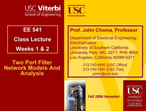
Overview of Lecture• Fundamental Types Of Filters• Frequency ResponseLowpassBandpassHighpassNotch• Constant Delay• Common Filter Characteristics• Maximum Voltage Or Current Transfer• Maximum Power TransferLossless Branch ElementsInput And Output Port Impedance Matching• Two Port Network Models• y-Parameters• z-Parameters• c-ParametersUSC Viterbi School of Engineering EE 536 Fall 2005 Lecture #02/Choma 2

• System Level Diagram And ResponseV s+−Z sIdeal Bandpass FilterZ in Z |H(j ω)|outV oV(jω)H(jω) oV(jω)sBandpassFilter• Basic Filter Properties• Constant “Gain” Within Filter Passband:⎛ B⎞ ⎛ B⎞H(jω) = H(jω ), ω ω ωo ⎜ −o ⎟ < < ⎜ +2o ⎟⎝ ⎠ ⎝ 2 ⎠• Zero “Gain” In Low And High Frequency Stopbands• Designable Passband Gain Or Attenuation, |H(jω o )|• Designable Bandwidth, B, And Center Or Tuned Frequency, ω o• Resultantly Designable Quality Factor: ωQ oBUSC Viterbi School of Engineering EE 536 Fall 2005 Lecture #02/Choma 4Z l|H(j ω o )|B0 ω o −B/2ω oω o +B/2ω

• System Level Diagram And ResponseV s+−Z sIdeal Highpass FilterZ in Z |H(j ω)|outV oV(jω)H(jω) oV(jω)sHighpassFilter• Basic Filter Properties• Constant “Gain” Within Filter Passband:• Zero “Gain” In Stopband: H(jω) = 0, ω < ωc• Designable Passband Gain Or Attenuation, |H(j∞)|• Designable Cutoff Frequency, ω c• Positive Real I/O Impedance RequirementRemains For This And All Other Passive FiltersZ l|H(j ∞)|0 ω cH(jω) = H(j ∞ ),ω > ωcωUSC Viterbi School of Engineering EE 536 Fall 2005 Lecture #02/Choma 5

• System Level Diagram And ResponseV s+−Z sZ in Z |H(j ω)|outV oV(jω)H(jω) oV(jω)sIdeal Notch FilterNotchFilter• Basic Filter Properties• Constant Attenuation Within Filter Stopband:⎛ B⎞ ⎛ B⎞H(jω) = H(jω ), ω < ω < ωo ⎜ −o ⎟ ⎜ +2o ⎟⎝ ⎠ ⎝ 2 ⎠• Constant “Gain” In Low And High Frequency Passbands• Designable Stopband Attenuation Factor, |H(jω o )| / |H(0)|• Designable Stopband Bandwidth, B, And Notch Frequency, ω o• Resultantly Designable Quality Factor:ωQ oBUSC Viterbi School of Engineering EE 536 Fall 2005 Lecture #02/Choma 6Z l|H(0)||H(j ω o )|B0 ω o −B/2ω oω o +B/2ω

• System Level Diagram And ResponseV s+−Z sH(jω)Z in Z φω ( )out0V oDelayFilter• Filter Delivers Linear I/O Phase Response• Significance Is Constant Time Delay Of Steady State SinusoidsV(jω) V cos ωt• Cursory Analysis:• Note Time DelayIn Steady StateIs FrequencyIndependentIdeal Delay FilterV(jω)oV(jω)s=H(jω)ejφ(ω)Z l( )s smV(jω) = H(jω)V (jω) = H(jω)V cos ωto s smV(jω) = H(jω)V cososm[ ωt + φ(ω) ]cos ω( )V(jω) = H(jω)V t −To sm dφ ω −ω( ) = T d( )ωUSC Viterbi School of Engineering EE 536 Fall 2005 Lecture #02/Choma 7

Filter Applications• Lowpass Filter• Mitigate Interference From High Frequency Signals• Integrate Applied Input Signal• Serve As Prototype For Other Filter Types• Bandpass Filter• Selective Signal Processing Over Stipulated Passband• Tuning In Communication Receivers• Highpass Filter• Mitigate Interference From Low Frequency Signals• Differentiate Applied Input Signal• Notch Filter Mitigate In Band Signal Interference• Delay Filter Incur Nominally Constant Time Delay InSinusoidal Steady StateUSC Viterbi School of Engineering EE 536 Fall 2005 Lecture #02/Choma 8

• Positive Real Impedances• Required For Stability• Required For Physically +VPossible Realizations• Mathematical ConstraintsRe ⎡Z (jω) ⎤ ≥ 0, for all ω ≥ 0⎣ in ⎦ReI/O Impedance Restrictions⎡Z (jω) ⎤ ≥ 0, for all ω ≥ 0⎣ out ⎦−Z sZ in Z outLinearV oPassive Filter• Signal Processing• Voltage Transfer |Z in (jω)| >> |Z s (jω)| ; |Z l (jω)| >> |Z out (jω)|• Current Transfer |Z in (jω)|

Positive Real Function Test• Generalized ImpedanceFunction (Constant K > 0)N(s)Z(s) = K = KD(s)N (s) + N (s)eeoD (s) + D (s)• Definitions• N e (s) / N o (s) Even/Odd Polynomial Components Of N(s)• D e (s) / D o (s) Even/Odd Polynomial Components Of D(s)• Positive Real (PR) Tests (3-Step Procedure)• Z(s) Must Be Real Number For All Real Values Of s (Satisfied IfAll s-Term Coefficients Are Real Numbers• N(s) + D(s) Must Be STRICTLY HURWITZThe Zeros Of N(s) + D(s) Must Lie In The Open Left Half s-Plane.If At Least One Zero Lies On The jω-Axis, N(s) + D(s) Is Said To BeA Hurwitz Polynomial.• Re[Z(jω)] ≥ 0 For All ω > 0• Satisfaction Of All Three Requirements Ensures Realization OfZ(s) As An Interconnection Of Passive ElementsoUSC Viterbi School of Engineering EE 536 Fall 2005 Lecture #02/Choma 10

Strictly Hurwitz Test• Auxiliary PolynomialQ(s) N(s) + D(s) = Q (s) + Q (s)• Continued Fraction Expansion• A Simple Exercise In Long DivisioneN(s)Z(s) = K = KD(s)Q(s)o1= cs+Q(s)11ec s +2 1 +c s• k Larger Of The Orders Of Q e (s) And Q o (s)• Strictly Hurwitz test Is Satisfied If:All c kAre Positive And Real NumbersThe Expansion Does Not Terminate Prior To the k th Term• Comments• Criteria Given Above Also Apply To Expansion Of Q e (s)/Q o (s)oN (s) + N (s)• The Even And Odd Nature Of Q e (s) and Q o (s) Render The DifferenceIn Order Of These Two Polynomial Components Precisely One• If Q e (s)/Q o (s) Were An Impedance, Expansion Suggests RealizationWith Exclusively Inductors And Capacitors; i.e. Lossless Elements.Parameter c 1 Is Inductance, c 2 Is Capacitance, etc.eeoD (s) + D (s)okUSC Viterbi School of Engineering EE 536 Fall 2005 Lecture #02/Choma 11

• Impedance FunctionN(s) N (s) + N (s) D (s) − D (s)Z(s) = K = Ke o×e oD(s) D (s) + D (s) D (s) − D (s)e o e oZ(s)=K⎡N (s)D (s) − N (s)D (s) ⎤ + ⎡N (s)D (s) − N (s)D (s) ⎤⎣ e e o o ⎦ ⎣ o e e o ⎦2 2D (s) − D (s)e o• First Bracketed Term In Numerator Is Even Function Of s; With sReplaced By jω, This Term Is Purely Real• Second Bracketed Term In Numerator Is Odd Function Of s; With sReplaced By jω, This Term Is Purely Imaginary• With s Replaced By jω, Denominator Is Positive, Real NumberN (jω)D (jω) − N (jω)D (jω)Ree e o o[ Z(jω) ] = K2 2D (jω) − D (jω)• Real Part Impedance• CriterionReal Part TestN (jω)D (jω) − N (jω)D (jω) ≥ 0, for all ω ≥ 0 and K > 0e e o oeoUSC Viterbi School of Engineering EE 536 Fall 2005 Lecture #02/Choma 12

Example Of Positive Real Test• Given Function• First TestZ(s)• Z(s) Must Be Real For All Real Values Of s• Satisfied Since Z(s) Is Real, Rational Function of s• Second Test• Expand Q e (s)/Q o (s)• Result Is Two Term ExpansionWith Positive Coefficients;• Passes Second Criterion• Third Test• Form IndicatedPolynomial• Satisfied SinceNo Value Ofe e o oFrequency ω Renders The Polynomial Negative.N(s) 6s + 17s + 6= =D(s) 3s + 1Q(s) = N(s) + D(s) = 6s + 20s + 72Q(s)e 6s + 7 3 1= = s +Q(s) 20s 10 20os7(2)N (s)D (s) − N (s)D (s) = 6s + 6 (1) −(17s)(3s)e e o o= 6 − 45sN (jω)D (jω) − N (jω)D (jω) = 6 + 45ω > 02222USC Viterbi School of Engineering EE 536 Fall 2005 Lecture #02/Choma 13

Ultimate Positive Real Test• Can Impedance Be Realized?26s + 17s + 6 1Z(s) = = 2s + 5 +3s + 1 3s + 1ImpedanceAdmittance• But How Does One Build A 2-NanohenrieInductance And A 3-Farad Capacitance?• For That Matter, Who Would Be Interested In An ImpedanceFunction Having A Self-Resonant Frequency Of 1 Radian/Sec?• No One Would Be Interested⎛ 1721+ s + s• The Indicated Impedance 6s + 17s + 6 ⎜Z(s) = = 6 ⎜6Has Evidently Been3s + 1 1 + 3sNormalized For Computational⎜⎝Convenience• Normalization Convenient From A Numerical PerspectiveZ(s)2H5Ω1Ω3F2⎞⎟⎟⎟⎠USC Viterbi School of Engineering EE 536 Fall 2005 Lecture #02/Choma 14

Parameter Normalization• Reference Variables• Let Impedance Be Normalized To An Impedance Value Of Z α• Let Inductance Be Normalized To An Inductance Value Of L α• Let Capacitance Be Normalized To A Capacitance Value Of C α• Let Frequency Be Normalized To A Frequency Value Of ω α• Let Time Be Normalized To A Time Value of t α• Resultant Normalized Z, L, C, ω, tZ L C ω tZ = L = C = ω = t =NZNLNCNωNtα α α α α• Normalized ResistanceR RZ = R → Z Z = R R → Z = ⇒ R = ZN αN α N α NZα ααThe Resistance Reference Value Is The Chosen ImpedanceReference ValueUSC Viterbi School of Engineering EE 536 Fall 2005 Lecture #02/Choma 15

Normalization . . . Cont’d• Normalized Inductance⎛ω L ⎞Z = jωL → Z Z = jω ω L L → Z = jω L ⇒ L =• Normalized Capacitance• Normalized Time⎜ α α ⎟N α N α N α N N N ⎜ Z ⎟ αα1 1 1⎛1⎞1Z = → Z Z = → Z = ⎜ ⎟ ⇒ C =jωCN αjω ω C CNjω C ⎜ω C Z ⎟ αω ZN α N α N N ⎝ α α α ⎠α α( )ωt = ω ω t t = ω t ω t ⇒ t =N α N α N N αα α• Note That Only Two Reference Variables Can BeChosen Independently1ωα⎝⎠ZωααUSC Viterbi School of Engineering EE 536 Fall 2005 Lecture #02/Choma 16

Normalization Example• Previous Impedance26s + 17s + 6 1Z(s) = = 2s + 5 +3s + 1 3s + 1Z(s)• Reference Variables• Time Reference (t α ) = 100 pSEC• Impedance Reference (Z α ) = 50 Ω• Normalized Parametric Variables• Normalized 1 RPS Is Actual 10 GRPS• Normalized 1 H Is Actual 5 nH• Normalized 1 F Is Actual 2 pF2HωLCααα5Ω1= =tαZ=α=ωααα1Ω1= =ω Z3F10 GRPS5 nH2 pFZ(s) 2HZ(s) 10 nH5Ω250 Ω50 Ω 6 pF1Ω3FUSC Viterbi School of Engineering EE 536 Fall 2005 Lecture #02/Choma 17

Short Circuit Y-ParametersY• Equations And Model⎡I 1⎤ ⎡y y V11 12⎤⎡1⎤⎢ ⎥ = ⎢ ⎥⎢ ⎥⎢I ⎥ ⎢y y ⎥⎢V⎥⎣ 2⎦ ⎣ 21 22⎦⎣ 2⎦• Independent Variables: V 1 , V 2• Dependent Variables: I 1 , I 2• Measurement• Short Circuited OutputYields y 11 , y 21• Short Circuited Input +VYields y 12 , yi22−• Bilateral Network Hasy 12 = y 21• All Passive Filters AreBilateralLinearTwo PortNetworkUSC Viterbi School of Engineering EE 536 Fall 2005 Lecture #02/Choma 181+V 1−21I 1+V1= Vi−211+V 1−2y 11I = y V1 11 i+V = 0−2I 1I = y V1 12 oy V 12 2LinearTwo PortNetworkLinearTwo PortNetworky V 21 1y 22I = y V2 21 iI = y V2 22 o3I 2V 2+−4I 2 3+V 2−3+V=20−4+V= V−1 2 o V o34+−4

Alternative Y-Parameter YModeling• Rewrite Characteristic Equations( ) ( )I = y V + y V = y + y V − y V −V1 11 1 12 2 11 12 1 12 1 2( ) ( ) ( )I = y V + y V = y − y V + y + y V − y V −V2 21 1 22 2 21 12 1 22 12 2 12 2 1• Bilateral Parametric Definitionsy = y + y y = y + yi 11 12 o 22 12y = y − y = 0 y = −yf 21 12 r 12• Bilateral Characteristic Equations( )I = yV + y V −V1 i 1 r 1 2( )I = y V + y V −V2 o 2 r 2 1• Results In Simple Pi-Type Model TopologyUSC Viterbi School of Engineering EE 536 Fall 2005 Lecture #02/Choma 19

• Model• Characteristic EquationsReflect BilateralRelationships• Elements y i , y r , And y oAre Any General PhysicalV sAdmittances That CoalesceTo Deliver Desired GainAnd Impedance Specs• Admittance/GainYinH(s)= y +iBilateral Pi—Type Model( + )y y Yr o ly + y + Yr o lV V V ⎛o i o 1⎞⎛ y ⎞= = × = ⎜ ⎟⎜ r ⎟V V V ⎜ 1+ Y Z ⎟⎜ y + y + Y ⎟s s i ⎝ in s ⎠⎝ r o l ⎠V s+−+−Z sZ sZ inZ inV iV iI 1I 2I 1LinearBilateralNetworky iy ry oI 2Z outZ outV oZ lV oZ lUSC Viterbi School of Engineering EE 536 Fall 2005 Lecture #02/Choma 20

• Presumptions• Z s = R s (Pure Resistance)• Z l = R l (Pure Resistance)• Desire Z in = Z s = R s• CommentsR sMay Be Characteristic+I 1 I 2Z inZ outy r V oV sy i y o−USC Viterbi School of Engineering EE 536 Fall 2005 Lecture #02/Choma 21Z sImpedance Of Transmission Line Coupling Of Media To ReceiverShunt Load Capacitance Or Inductance Can Be Absorbed Into y oSeries Load Inductance Or Capacitance Requires Another Filter ModelInput Port Match To Source Resistance Effects Maximum Power Transfer• Gain And Input AdmittanceH(s)Plausible Design StrategyV ⎛o 1⎞⎛ y ⎞r 1⎛ y ⎞⎛ ⎞= = ⎜ ⎟⎜ ⎟ = ⎜ r ⎟V ⎜ ⎜ ⎟1+ Y Z ⎟⎜ y + y + Y ⎟ ⎝2⎠⎜ y + y + G ⎟s ⎝ in s ⎠⎝ r o l ⎠ ⎝ r o l ⎠( + )y y Gr o l( )1Y = y + = y + 2H(s) y + G ≡in iy + y + Gi o lRr o l sV iZ l

• Desired TransferFunction• Second Order Maximally FlatH(s)H(s)Magnitude (more about this later)• 3-dB Bandwidth Is ω o• Recast Gain Function• Determine y r• Determine y r + y o• Determine y oyrSecond Order Lowpass Filter⎡2N (s) ⎤= ⎢ e ⎥G=⎢ D(s) ⎥ l⎣ o ⎦2KωRsloK= =22s⎛s⎞1 + + ⎜ ⎟ω ⎜ ω ⎟o ⎝ o ⎠⎡ ⎤D(s)N (s)⎢ e ⎥ G⎢D(s)⎥ lo1⎛ y ⎞⎣ ⎦ ⎛ ⎞⎜ r ⎟D(s) ⎝2⎠ y y Ger o l+ ⎥ ⎝ ⎠D(s) ⎥ lo= =⎡ ⎤⎜ ⎟⎜+ + ⎟⎢1 G⎢⎣ ⎦eN (s)⎡⎛s⎞⎤⎢ ⎥1 + ⎜ ⎟⎢ ⎥ω⎡ ωD(s) ⎤⎜ ⎟⎢ ⎝ o ⎠ ⎥y + y = ⎢ e ⎥G=⎣ ⎦r o ⎢D(s)⎥ l2Rs⎣ o ⎦l2e+D(s)ooUSC Viterbi School of Engineering EE 536 Fall 2005 Lecture #02/Choma 22

Lowpass Filter Design . . . Cont’d• Shunt Output Admittance• For Physical Realizability, 2K ≤ 1• Pick K =1/2 For Topological Simplicityy⎡ωo ⎢y =o ⎢( 1− 2K)+2R sl ⎢⎣• Resultant y r And y o Realizations• Resultant y i Realization• Necessary Condition For RealizabilityIs G s ≥ G l , Or R s ≤ R l• Known As A Filter “Down Converter” In The SenseThat It Transforms A Load Resistance Into A Smaller Or EqualMatched Source ResistancesG( )2s⎛l⎞ sG 1+ G − G + G − + Gl2ωs l ω ⎜ s 2 ⎟ sωo o ⎝ ⎠ o= G − =i s 2 22 R lω o⎛ ⎞ ⎛ ⎞⎜ ⎟ ⎜ ⎟⎜ ⎟ ⎜ ⎟⎝ ⎠ ⎝ ⎠2s⎛s⎞2s⎛s⎞1+ + ⎜ ⎟ 1+ + ⎜ ⎟ω ⎜ω ⎟ ω ⎜ω⎟o ⎝ o ⎠ o ⎝ o ⎠2⎛s⎞⎤⎜ ⎟⎥⎜⎥ω ⎟⎝ o ⎠ ⎥⎦y ry 1o2 R lω o2USC Viterbi School of Engineering EE 536 Fall 2005 Lecture #02/Choma 23

Lowpass Filter Design . . . Cont’d• Admittance y i• Continued Fraction Expansion Is Formidable Algebraic Problem• Consider Simplifying Case Of R s = R l2Gs ⎛s s⎞+ G ⎜ ⎟2ωs ⎜ω ⎟o o1y =⎝ ⎠=i 2 2R ω2s⎛s⎞s o 11 + + ⎜ ⎟+s 1 ωω ⎜ ω ⎟ oo ⎝ o ⎠+R 2R ss sy i• Realization of y i12 R sω oRs2 R sω oUSC Viterbi School of Engineering EE 536 Fall 2005 Lecture #02/Choma 24

Lowpass Filter Design . . . Cont’d• Final Topological RealizationZ(s) in = Rs• CharacteristicsV i• 2 nd Order Maximally FlatMagnitude Response• Input Impedance IsNominally Constant AtRsValue Of R s• 3-dB Bandwidth Is ω o• Cursory Check12 R sω o2 R sω o2 R sω o12 R sω o• At High Frequencies Where Inductances Are Open Circuits AndCapacitors Are Short Circuits, Z in (s) = R s , By Inspection• At Low Frequencies Where Capacitances Are Open Circuits AndInductors Are Short Circuits, Z in (s) = R s , By Inspection• Ultimate Check Is HSPICE Simulation For Given R s And ω oV oR sUSC Viterbi School of Engineering EE 536 Fall 2005 Lecture #02/Choma 25

HSPICE Verification Of Design• Design• R s = 50 Ω• ω o = 2Π(1 GHz)• 50 Ω, 1 V Signal• Simulations• Confirmed1 GHz BandwidthFlat FrequencyResponseFlat Input PortVoltage Is ½That Of InputSignal VoltageLatter Confirms50 Ω InputImpedance ForAll Frequencies50 Ω1 VACZ(s) in = Rs+−V iV iINRs50 Ω12 R sω o2.251 pF11.25 nH2 R sω o2 R sω o11.25 nH12 R sω oOUT2.251 pFV oV oR s50 ΩUSC Viterbi School of Engineering EE 536 Fall 2005 Lecture #02/Choma 26

HSPICE Simulation Results• Small Signal AC Simulations353.6 mV3-dB BandwidthUSC Viterbi School of Engineering EE 536 Fall 2005 Lecture #02/Choma 27

Open Circuit z-Parametersz• Equations And Model⎡V 1⎤ ⎡z z11 12⎤⎡I1⎤⎢ ⎥ = ⎢ ⎥⎢ ⎥⎢V z z I⎣ 2⎥⎦ ⎢⎣ 21 22⎥⎢ ⎦⎣ 2⎥⎦• Independent Variables: I 1 , I 2• Dependent Variables: V 1 , V 2• Measurement• Open Circuited OutputYields z 11 , z 21• Open Circuited InputYields z 12 , z 22• Bilateral Network Hasz 12 = z 21• z-matrix Is Inverse Ofy-matrix For A GivenLinear Network+V 1−2I 1LinearTwo PortNetworkUSC Viterbi School of Engineering EE 536 Fall 2005 Lecture #02/Choma 281+V 1−211z 11I 1+−z I 12 2+z21 I1−3I 2+V 2−4I 2 3z 22+V 2−I 1I2= 0+ Linear+V1= z11 I1 Two Port V2= z21 I1− Network −241 I1= 03++V1= z12 I2V2= z22 I2I 2−−2LinearTwo PortNetwork344

Alternative z-Parameter zModeling• Rewrite Characteristic Equations( ) ( )V = z I + z I = z − z I + z I + I1 11 1 12 2 11 12 1 12 1 2( ) ( ) ( )V = z I + z I = z − z I + z − z I + z I + I2 21 1 22 2 21 12 1 22 12 2 12 1 2• Bilateral Parametric Definitionszi= z − z11 12zo= z − z22 12zf= z − z21 12= 0 zr= z12• Bilateral Characteristic Equations( )V = z I + z I + I1 i 1 r 1 2( )V = z I + z I + I2 o 2 r 1 21+V 1−2I 1• Results In Simple Tee-Type Model Topologyz 11+−z I 12 2+z21 I1−z 22I 23+V 2−4USC Viterbi School of Engineering EE 536 Fall 2005 Lecture #02/Choma 29

• Model• Characteristic EquationsReflect BilateralRelationships• Elements z i , z r , And z oAre Any General PhysicalV sImpedances That CoalesceTo Deliver Desired GainAnd Impedance Specs• Impedance/GainZinH(s)= z +iBilateral Tee-Type Type Model( + )z z Zr o lz + z + Zr o lV sV V I I ⎛ Z ⎞⎛ z ⎞=o=o×2× 1= ⎜ l ⎟⎜ r ⎟V I I V ⎜ Z + Z ⎟⎜ z + z + Z ⎟s 2 1 s ⎝ s in ⎠⎝ r o l ⎠+−+−Z sZ sZ inZ inV iV iLinearBilateralNetworkI 1I 2I 1I 2ziz rz oZ outZ outV oZ lV oZ lUSC Viterbi School of Engineering EE 536 Fall 2005 Lecture #02/Choma 30

• Presumptions• Z s = R s (Pure Resistance)• Z l = R l (Pure Resistance)• Desire Z in = Z s = R s• CommentsR sMay Be CharacteristicZ sV iI 1I 2ziz rz oZ in Z outV o+V sZ−lImpedance Of Transmission Line Coupling Of Media To ReceiverSeries Load Inductance Or Capacitance Can Be Absorbed Into z oInput Port Match To Source Resistance Effects Maximum Power Transfer• Gain And Input ImpedanceH(s)Filter Design StrategyV ⎛ R ⎞⎛ z ⎞=o= ⎜ l ⎟⎜ r ⎟V ⎜ 2R ⎟⎜ z + z + R ⎟s ⎝ s ⎠⎝ r o l ⎠( + )z z R ⎛2R⎞Z z z H(s) z R R( )r o l= + = + ⎜ s ⎟ + ≡in iz + z + Ri ⎜ R ⎟ o l sr o l l⎝⎠USC Viterbi School of Engineering EE 536 Fall 2005 Lecture #02/Choma 31

• Volt-Ampere Equations⎡V 1⎤ ⎡c c11 12⎤⎡V2⎤⎢ ⎥ = ⎢ ⎥⎢ ⎥⎢I c c −I⎣ 1⎥⎦ ⎢⎣ 21 22⎥⎢ ⎦⎣ 2⎥⎦• ParametricMeasurement• RelationshipTo z-Parametersc11c2122Transmission ParametersV z= 1 = 11V z2 I = 0 21I1 1= =V z2 I = 0 21c22Ideal TestVoltage SourceIdeal TestCurrent Source+−LinearTwo PortNetworkUSC Viterbi School of Engineering EE 536 Fall 2005 Lecture #02/Choma 32+−1+V 1−21+V 1−I z= − 1 = 22I z2 V = 0 2122I 1I 11+I 1LinearTwo PortNetworkLinearTwo PortNetworkZ sV sV 1V 2 Z l−22I = 02V = V /c= I /cI = −I /c2 1 112 1 22= −V /c1 12I 21 2143+−43+V=20−43+−OpenCircuitShortCircuitV z zc = −1=11 22− z12Iz122 V = 0 21

c-Parameter Network Properties• c-Matrix Determinant• Equals Zero For No Feedback• Equals One For Bilateral Network• Input Impedance +Z (s)inZ (s)inV c V − c I= 1 = 11 2 12 2I c V − c I1 21 2 22 2V c Z + c= 1 =11 l 12I c Z + c1 21 l 22• Output ImpedanceZ (s)outV c Z + c= 2 =22 s 12I c Z + c2 21 s 11−∆1+= c c − c c =c 11 22 12 21I 1LinearTwo PortNetworkz12z21Z sV sV 1V 2 Z l−2Z(s)in● Voltage TransferI 23+−4Z (s)out⎛V⎞V = c V − c I = c V + c ⎜ 2 ⎟1 11 2 12 2 11 2 12⎜Z ⎟⎝ l ⎠V Z2=l H (s)V c Z + c211 11 l 12USC Viterbi School of Engineering EE 536 Fall 2005 Lecture #02/Choma 33

Comments On Transfer Properties• Large Load Impedance• Output Current (I 2 ) Is Zero• Load (Z l ) Absorbed Into Filter• Resultant BilateralMatricH (s)21Z (s)inV Z2l1= = =V c Z + c c1 Z 11 l 12 Z 11→∞l⎡ 1Z (s) ⎡c H (s) ⎤⎤⎢−V H (s)in ⎣ 22 21 ⎦⎥⎡1⎤ ⎢ 21⎥⎡V2⎤⎢ ⎥ =I⎢1⎥⎢ ⎥⎢⎣ 1 ⎥⎦ ⎢0c ⎥⎣ − ⎦⎢H (s)Z (s)22 ⎥⎣ 21 in⎦c Z + c c=11 l 12=11c Z + c c21 l 22 Z →∞ 21• Second Column Multiplies Only Null Current At Output Port• Can Arbitrarily Set c 22 = H 21 (s)• Resultant c 12 Is Zerol→∞lUSC Viterbi School of Engineering EE 536 Fall 2005 Lecture #02/Choma 34

Cascade Network Interconnection• Two StageCascade• V-I TransferI 1 I 1I o1 3I 2 5i2+ Linear + Linear +V 1Two Port V xTwo Port V 2− Network (A) − Network (B) −246⎡V1⎤ ⎡ Vx⎤ ⎡Vx⎤ ⎡V2⎤⎢ ⎥ = C ⎢ ⎥ ⎢ ⎥ = C ⎢ ⎥I A I I B⎢ −−I⎣ 1⎥⎦ ⎢⎣ 01⎥⎦ ⎢⎣ i2⎥⎦⎢⎣ 2⎥⎦⎡V V VV V1⎤ ⎡x⎤ ⎡x⎤ ⎡2⎤ ⎡2⎤⎢ ⎥ = C ⎢ ⎥ = C ⎢ ⎥ = C C ⎢ ⎥ ≡ C ⎢ ⎥I A I A I A B⎢ − −I −I⎣ 1⎥⎦ ⎢⎣ 01⎥⎦ ⎢⎣ i2⎥⎦⎢⎣ 2⎥⎦ ⎢⎣ 2⎥⎦• Can Be Extended To Multistage Cascade• Overall Transmission Matrix Derives From The OrderedMultiplication Of The Transmission Matrices For The IndividualConstituents Of The Overall Network Cascade• Note That Ordered Matrix Multiplication Is CrucialUSC Viterbi School of Engineering EE 536 Fall 2005 Lecture #02/Choma 35

• Generalized V-I Equations• Series Branch ElementI 1Z⎡V⎤ ⎡1 Z⎤⎡V⎤⎢ ⎥ ⎢ ⎥⎢⎣ ⎥⎦ ⎢⎣ ⎥⎦I 2+ + 1 2V 1 V 2=I⎢0 1⎥I− − 1 ⎣ ⎦ −2• Parallel Branch Element+I 1V 1Y V 2−I 2⎡V+ 1⎤ ⎡1 0⎤⎡V2⎤⎢ ⎥ =I⎢Y 1⎥⎢ ⎥I−⎢ −⎣ 1⎥⎦ ⎣ ⎦⎢⎣ 2⎥⎦• Three Element CascadeCSeries And Shunt Branches⎡V 1⎤ ⎡c c11 12⎤⎡V2⎤⎢ ⎥ = ⎢ ⎥⎢ ⎥⎢I c c −I⎣ 1⎥⎦ ⎢⎣ 21 22⎥⎢ ⎦⎣ 2⎥⎦Note: This Is A CascadeOf Three Networks, EachOf Which Consists Of ASingle Branch ElementI 1Z 1Z 3++V 1Y 2 V 2−−{ ( )}⎡1 Z1⎤⎡ 1 0⎤⎡1 Z 1 Y Z Z Z 1 Y Z3⎤⎡ + + += ⎢ ⎥⎢0 1 Y 1⎥⎢ ⎥ = ⎢⎣ ⎦⎣ 2 ⎦⎣⎢0 1 ⎥ ⎦⎢ Y 1+Y Z⎣ 2 2 32 1 3 1 2 3⎤⎥⎥⎦I 2USC Viterbi School of Engineering EE 536 Fall 2005 Lecture #02/Choma 36