Doppler sonar observations of Langmuir circulation - Jerry Smith's ...

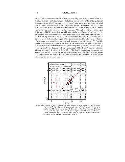
550 JEROME A. SMITHrelation. It is wise to examine the relation on a case-by-case basis, to see if there is a“hidden” relation. Unfortunately, as noted above, only events 2 and 3 of the potential5 segments from SWAPP provide both a “clean” wind event (not confused by windveering) and a wide range of U S /u*. These two events (henceforth “SWAPP-2” and“SWAPP-3”) are plotted together with the “MBLEX-1” event in Figure 19.10. Theseregressions support the value n=1 for the exponent. Although the fits are not as tightas for the MBLEX-1 data, they are still statistically significant at well over 95%.Intriguingly, there is considerable offset between the lines, especially between SWAPPand MBLEX (by a factor of about 5), but also between the two SWAPP events (by afactor of about 2). Some other aspect of the environment must be affecting the relation.What could be responsible for the observed variation in velocity scale V rms ? Possiblecandidates include variations of scaled depth of the mixed layer kh, effective viscosityν t , a directional effect of the horizontal Coriolis component [Cox and Leibovich 1997],or suppression by the buoyancy of the near-surface bubble cloud. A summary of somerelevant parameters is given in Table 19.1. The first 6 parameters summarize theobservations for the 3 events; the rest are derived from these. An effective wave periodT S is derived from the surface Stokes’ drift, assuming the variations in mean-squarewave steepness are not very large:9Red crosses: no LCBlack circles: LC identified5V rms /u*21Slope = 1.001 ±0.034r2 = 0.8860.52 5 10U s 20/u*Figure 19.8 Scaling of the rms measured radial surface velocity takes the general formV~u*(U s /u*) n . The value of n is sought as the slope of (V/u*) versus (U s /u*) on alog-log plot. This figure indicates a well-determined value for n very near 1.0; i.e.,V ~ U s , with no dependence on u* once Langmuir circulation is well formed.Values before year day 67.66, when there were no signs of Langmuir circulation,are shown as red crosses but not included in the fit.