Tunnel-MILP: Path Planning with Sequential Convex ... - Michael Vitus

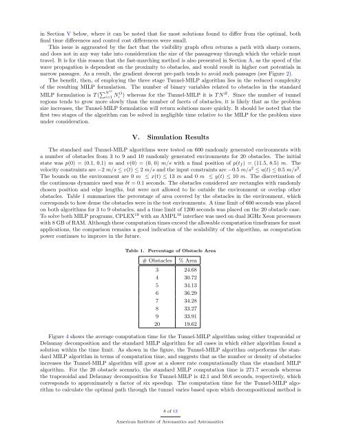
in Section V below, where it can be noted that for most solutions found to differ from the optimal, bothfinal time differences and control cost differences were small.This issue is aggravated by the fact that the visibility graph often returns a path with sharp corners,and does not in any way take into consideration the size of the passageway through which the vehicle musttravel. It is for this reason that the fast-marching method is also presented in Section A, as the speed of thewave propagation is dependent on the proximity to obstacles, and would result in higher cost potentials innarrow passages. As a result, the gradient descent pre-path tends to avoid such passages (see Figure 2).The benefit, then, of employing the three stage Tunnel-MILP algorithm lies in the reduced complexityof the resulting MILP formulation. The number of binary variables related to obstacles in the standardMILP formulation is T ( ∑ N Oi=1 N i O) whereas for the Tunnel-MILP it is T N R . Since the number of tunnelregions tends to grow more slowly than the number of facets of obstacles, it is likely that as the problemsize increases, the Tunnel-MILP formulation will return solutions more quickly. It should be noted that thefirst two stages of the algorithm can be solved in negligible time relative to the MILP for the problem sizesunder consideration.V. Simulation ResultsThe standard and Tunnel-MILP algorithms were tested on 600 randomly generated environments witha number of obstacles from 3 to 9 and 10 randomly generated environments for 20 obstacles. The initialstate was p(0) = (0.1, 0.1) m and v(0) = (0, 0) m/s with a final position of p(t f ) = (11.5, 8.5) m. Thevelocity constraints are −2 m/s ≤ v(t) ≤ 2 m/s and the input constraints are −0.5 m/s 2 ≤ u(t) ≤ 0.5 m/s 2 .The bounds on the environment are 0 m ≤ x(t) ≤ 13 m and 0 m ≤ y(t) ≤ 10 m. The discretization ofthe continuous dynamics used was δt = 0.1 seconds. The obstacles considered are rectangles with randomlychosen position and edge lengths, but were not allowed to lie outside the environment or overlap otherobstacles. Table 1 summarizes the percentage of area covered by the obstacles in the environment, whichcorresponds to how dense the obstacles were in the test environments. A time limit of 600 seconds was placedon both algorithms for 3 to 9 obstacles, and a time limit of 1200 seconds was placed on the 20 obstacle case.To solve both MILP programs, CPLEX 19 with an AMPL 18 interface was used on dual 3GHz Xeon processorswith 8 GB of RAM. Although these computation times exceed the allowable computation timeframes for mostapplications, the comparison remains a good indication of the scalability of the algorithm, as computationpower continues to improve in the future.Table 1.Percentage of Obstacle Area# Obstacles % Area3 24.684 30.725 34.136 36.297 34.288 33.279 33.9120 19.62Figure 4 shows the average computation time for the Tunnel-MILP algorithm using either trapezoidal orDelaunay decomposition and the standard MILP algorithm for all cases in which either algorithm found asolution within the time limit. As shown in the figure, the Tunnel-MILP algorithm outperforms the standardMILP algorithm in terms of computation time, and suggests that as the number or density of obstaclesincreases the Tunnel-MILP algorithm will grow at a slower rate computationally than the standard MILPalgorithm. For the 20 obstacle scenario, the standard MILP computation time is 271.7 seconds whereasthe trapezoidal and Delaunay decomposition for Tunnel-MILP is 42.1 and 50.6 seconds, respectively, whichcorresponds to approximately a factor of six speedup. The computation time for the Tunnel-MILP algorithmto calculate the optimal path through the tunnel varies based upon which decompositional method is8 of 13American Institute of Aeronautics and Astronautics