Lectures on Fractional Calculus - CARMA

Three <strong>Lectures</strong> on the FractionalCalculusRoss McPhedran,ross@physics.usyd.edu.au

• Motivation, history• Fractional calculus of one variableOutline• Fourier transforms, Green’s functions anddistributions• Laplacian in two dimensions to an arbitrarypower

References• A child’s garden of fractional derivatives, MarciaKleinz and Tom Osler• Mathematica for theoretical physics, Gerd Baumann,Springer 2004, Chapter 7.• Fractional kinetics, I.M .Solokov, J. Klafter and A.Blumen,Physics Today, November 2002, pp. 48-54• Electromagnetic processes in dispersive media, D.B. Melrose and R.C. McPhedran, CambridgeUniversity Press 2005, Chapters 4,5.

Motivation, History• In the late 17 th century calculus hadtransformed mathematics and physics- wherewere its boundaries?• Letter from Leibnitz to l’Hospital: Can themeaning of derivatives with integral order n betransformed to non-integral, even complex,orders?• Difficulties arose: Leibnitz: Il y a del’apparence qu’on tirera un jour desconsequences bien utiles de ces paradoxes,car il n’y a gueres de paradoxes sans utilite

Motivation, History (2)• Initial motivation: curiosity. Major contributionsfrom Liouville, Riemann, Laplace, Heaviside,Weyl, etc• Well established mathematical frameworknow finding applications• Differentiation makes functions nastier;integration makes them better; fractionaldifferentiation can make them “just right”. Seethe Physics Today article.

Scope of Fractional Calculus• Differentiation with respect to arbitrarypowers: they can be negative• Negative differentiation is integration• Integration needs two limits to have a precisemeaning• Fractional derivatives in general need a lowerlimit, and a variable indicated Da,xαα- orderofdifferentiation or integrationa lower limit; x variable

Fractional Differentiation (1)d n x mdx n = m!(m−n)! xm−nm! =Γ(m +1)d n x mdx n = Γ(m+1)Γ(m−n+1) xm−n• This is the Riemann-Liouville derivative.• Can be applied to functions representedby Taylor series• n can be any real or complex number

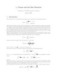
Fractional Differentiation (2)d n x mdx n = Γ(m+1)Γ(m−n+1) xm−n1Γ(x)x• The result will be zero ifm-n+1 is zero or anegative integer;• Otherwise its non-zerom =0:d n 1dx n = x−nΓ(1−n)e.g.d 1/2 1dx 1/2 = 1 √ πx

Factorial FunctionKey equations for the gamma function are:Γ(z +1)=zΓ(z) =z! =z(z − 1)!, (1)Γ(1) = 1, (2)Γ(z) = R ∞t z−1 e −t dt, 0, (3)0andΓ(z)Γ(1 − z) =πsin(πz) . (4)From (4) one can prove other useful things-e.g.,Γ(1/2) = √ π (5)andΓ(−n + δ) = (−1)nn!δ . (6)

Fractional Differentiation (3)d n x mdx n = Γ(m+1)Γ(m−n+1) xm−n¡d p d¢ n x mdx p dx =Γ(m−n+1)n Γ(m−n−p+1)Γ(m+1)Γ(m−n+1) xm−n−pi.e.¡d p d¢ n x mdx p dx =Γ(m+1)n Γ(m−n−p+1) xm−n−pExample:³d 1/2dx 1/2d 1/2 1dx 1/2 ´=Γ(1)Γ(1−1/2−1/2) x−1 =0

A Fractional DifferentiationConundrumWeknowforanyintegern:D n (e ax )=a n e axso we want for any αD α (e ax )=a α e ax .Yet:D α e x = D α ( P ∞n=0 xnn! )=P ∞n=0x n−αΓ(n−α+1)These don’t match unless α is an integer!

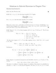
Integration as Negative Differentiationt 2t 1t 1xxt 2t 2t 1We consider the definite integrals:D −1 f(x) = R x0 f(t)dt, D−2 f(x) = R x R t20 0 f(t 1)dt 1 dt 2 .In the second integral, we invert the order of integrations,going from left to right diagrams above.D −2 f(x) = R x R x0 t 1f(t 1 )dt 2 dt 1 = R x0 f(t 1)(x − t 1 )dtR 1D −3 f(x) = 1 x2 0 f(t 1)(x − t 1 ) 2 dtR 1D −n f(x) = 1 x(n−1)! 0 f(t 1)(x − t 1 ) n−1 dt 1

Integration as NegativeDifferentiation(2)We generalize RD −n f(x) = 1 x(n−1)! 0 f(t 1)(x − t 1 ) n−1 dt 1to give RD −α f(x) = 1 xΓ(α) 0 f(t 1)(x − t 1 ) α−1 dt 1For the singularity at t 1 → x to be integrable, we requireα > 0, confirming we are dealing with a negative order ofdifferentiation.So we write our generalized differential operator with acurly D, putting its order as the superscript,and the lower limit and variable being differentiatedas subscripts. The two usual choices for lowerlimits are 0 and −∞.D α a,x

Integration as NegativeDifferentiation(3)Being clear about implicit limits enables us to clear up theprevious difficulty:D −1b,x eax = R xb eax dx = eaxaif b = −∞D −1b,x xp = R xb xp dx = xp+1p+1if b =0For any given physical problem, there will be a choiceto make about the best value of lower limits.This choice will control the results of differentiationsto fractional powers.D0,x(x α p )= Γ(p+1)xp−αΓ(p−α+1)andD−∞,x(e α ax )=a α e ax

Differentiation as Negative IntegrationWe can define fractional differentiation on the basisof fractional integrationDa,x s =( dndx)D −(n−s)n a,x f(x)with n a positive integer, 0, 0.We have then some familiar properties- linearity:Da,x(αf(x)+βg(x)) s = αDa,xf(x)+βD s a,xg(x)sand compositionDa,xD s a,xf(x) p =Da,x s+p f(x),with p0, see Baumann.For Leibnitz’s rule, we get an infinite series:Da,x(f(x)g(x)) q = P µ ∞ qj=0Dja,x q−j f(x)Da,xg(x),jwith the symbol in brackets beingΓ(q +1)/(Γ(j +1)Γ(q − j + 1)).

• Reprise from last lecture:Lecture 2- Fourier methodsd p x qdx= D p p 0,x = Γ(q+1)Γ(q−p+1) xq−pthe Riemann-Liouville derivative.Differentiation to a negative power:Da,x −αf(x)= R 1 xΓ(α) a f(t 1)(x − t 1 ) α−1 dt 1for α > 0.Most discussions use fractional calculus in onevariable. Let’s see how we can treat two dimensions,using Fourier transform ideas.

Adding up Harmonics• Fourier series- sines and cosines adding up togive arbitrary waveforms: harmonics• Fourier transforms- not just harmonics, but anintegral over all frequencies• In more than one dimension, add up planewaves• In two dimensions, a plane wave isexp i(k x x + k y y)Wave vector:(k x ,k y )=k, momentum ¯hk

The Fourier transform• Represent a function in space as an integralover plane waves: inverse transformA(x) =A(x, y) = R dk x dk y(2π) 2 e i(k xx+k y y) Ã(k x ,k y )Function inspaceFunction in wave vectorspace; reciprocal space;momentum spaceDirect transform:Ã(k x ,k y )= R dxdye −i(k xx+k y y) A(x, y)

Momentum space• A lot of physics is based on momentum orwavevector space• Conservation of momentum: p =¯hk• A mathematical reason: derivatives arereplaced by algebraic operationsA(x) =A(x, y) = R dk x dk y(2π) 2 e i(k xx+k y y) Ã(k x ,k y )∂∂x A(x) =R dk x dk y(2π) 2 e i(k xx+k y y) ik x Ã(k x ,k y )∂∂xPartial derivative with respect to x

The Laplacian• A particularly important operator in physics isthe Laplacian• Take two derivatives with respect to x, twowith respect to y and add• Crops up in electrostatics, magnetostatics,complex variable theory• Symbol:∇ 2 = ∂2∂x 2∂ 2∂x 2→−k 2 x+ ∂2∂y 2 ∂ 2∇ 2 →−(k 2 x + k 2 y)∂y 2→−k 2 y

The Laplacian (2)Once:n times:∇ 2 →−(k 2 x + k 2 y)∇ 2n → (−1) n (k 2 x + k 2 y) np timessince∇ 2p → e iπp (k 2 x + k 2 y) p(−1) n =cos(nπ)+i sin(nπ) =e iπn∇ 2p A(x, y) → e iπp (k 2 x + k 2 y) p Ã(k x ,k y )

The Dirac delta function• Fourier transforms integrate over extendedobjects: plane waves• Need a way of going from extended objects topoint-like objects• This is provided by the Dirac delta function:the Fourier transform of a constant2πδ(ω) = R ∞−∞ dteiωt(2π) 2 δ 2 (k x ,k y )= R ∞−∞ dxdyei(k xx+k y y)Delta function of angularfrequencyDelta function of wavevector (2D)

The Dirac delta function (2)• The more spread out a function is, the tighterits Fourier transform concentrates around theorigin• A constant is spread out uniformly in space:its Fourier transform concentrates around theorigin in reciprocal space• Another way of thinking about the deltafunction is that it is a function concentratedaround the origin, but having unit area underits curve

The Dirac delta function (3)• One representation is based on Gaussianfunctionsf T (t) =e −t2 /T 2δ(ω) =lim T →∞→T2 √ π e−ω2 T 2 /4Function → constantTransform→ deltaf T (t)δ T (ω)T =10

Green’s functions• A Green’s function for a problem in physics isa solution of the governing equationcorresponding to a point source• The point source is just a delta function• So for example in electrostatics if we look forthe Green’s function for a point source at theorigin, we want to solve∇ 2 G(x, y) =−δ 2 (x, y)The minus sign is just a convention: other authorshave a plus sign

Green’s functions (2)• Once you have the Green’s function for apoint source, you can get the solution for anarbitrary set of sources by summing theGreen’s function multiplied by the strength ofthe source• You know well the potential for a pointelectrostatic charge in 3D:G(x, y, z) = 14πr , r = p x 2 + y 2 + z 2

The Green’s function in 2DWe start with(2π) 2 δ 2 (k x ,k y )= R ∞−∞ dxdyei(k xx+k y y)and∇ R 2 ∞−∞ dxdyei(k xx+k y y) =− R ∞−∞ dxdy(k2 x + k 2 y)e i(k xx+k y y)HenceG(x, y) = 14π 2 R ∞−∞R ∞−∞e i(k xx+ky y)(k 2 x +k2 y )Theintegralisdoneinpolarcoordinates:k x = r cos(θ), k y = r sin(θ).

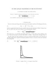
G(x, y) = 14π 2 R ∞−∞R ∞−∞The Green’s function in 2D (2)e i(k xx+ky y)(k 2 x +k2 y )In R polar coordinates, the angular integral is:π−π exp(ikr cos θ) =2πJ 0(kr).Here J 0 (z) is theBessel function of order zero(of the first kind).This gives usR ∞0G(x) =G(r) = 12πdk J 0(kr)k.If we require that G(r) vanishatr = a, wegetG(r) = 12πR ∞0dk J 0(kr)−J 0 (ka)k.

R ∞0The Green’s function in 2D (3)G(r) = 12πdk J 0(kr)−J 0 (ka)k.We evaluate this using Frullani’s integralI(a, b) = R ∞dx [f(ax)−f(bx)]0 x, a>0,b>0and f(x) iscontinuousatx =0. ThenI(a, b) =f(0) ln(b/a).HenceG(r) = 12π ln ¡ ¢ar .This is the 2D Green’s function. It satisfies∇ 2 G(r) =−δ 2 (x), |x| = r.

Lecture 3- Green’s Functions forFractional OperatorsG(r) = 12π ln ¡ ¢ar .This is the 2D Green’s function. It satisfies∇ 2 G(r) =−δ 2 (x), |x| = r.Thequestionweanswerhereis:What does this Green’s function become ifwe want to have the operator ∇ 2s ,s arbitrary real or complex?

A Neat TrickWe know the Green’s function for the Laplacian:G 2 (r) =− 12π ln(r)gives∇ 2 G 2 (r) =−δ 2 (x, y)We want to know what G 2s is for which∇ 2s G 2s (r) =−δ 2 (x, y)We write∇ 2 G 2 (r) =∇ 2s (∇ 2−2s G 2 (r))Then quite simply:G 2s (r) =∇ 2−2s G 2 (r)So all we need is to apply the Laplacian to an arbitrarypower to the log function!

Technical Details (1)To carry out this calculation, we first need to know∇ 2s r β . It is obvious that each secondderivative reduces the power of r by 2, so∇ 2s r β = K(r, β)r β−2sfor some K(s, β) which depends on β and s,but not r.To evaluate K(s, β) we need Weber’s integral:R ∞0r s J 0 (αr)dr =Γ(1+s2 )2sΓ( 1−s2 )α1+s

Technical details (2)We write down the Fourier transform of r β :r β = R ∞ R ∞ Γ(1+β/2)e 2πi(k xx+k y y) dk−∞ −∞ Γ(−β/2)π β+1 k β+2 x dk y .To check this expression, convert the double integral toan integral over angle multiplied by an integral over kdk.The integral over angle gives the Bessel function2πJ 0 (2πkr). You then get2Γ(1+β/2)R ∞k −1−β dkJΓ(−β/2)π β 00 (2πkr).You then use Weber’s integral to verify the result.

Differentiation of the Logarithm∇ 2s (r β )=i 2s 2 2s Γ(1+β/2)Γ(−β/2)Γ(s−β/2)Γ(1−s+β/2) rβ−2sSuppose we expand this taking β small:r β = e β ln r ' 1+β ln r.Then this will tell us how ∇ 2s operates on a constant and ln r.The only term which causes any problem is1Γ(z) ' z, for |z|

• So we have deduced:G 2s (r) = −r2s−2 Γ(1−s)π(2i) 2s Γ(s)Only for s→ 1 will we get a logarithm!Γ(s)Γ(1−s) r−2s ,∇ 2s (ln r) ' −i 2s 2 2s−1so that∇ 2−2s (ln r) ' −i 2−2s 2 2−2s−1 Γ(1−s)Γ(s)r −2+2sThe Final AnswerWe have also learned that Fourier transforms can beused as a way of evaluating fractional derivatives.