Shear viscosity and dielectric constant of liquid acetonitrile

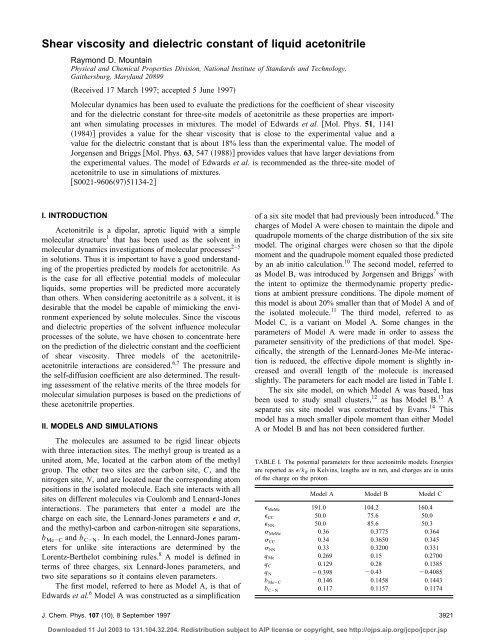
Shear viscosity and dielectric constant of liquid acetonitrileRaymond D. MountainPhysical and Chemical Properties Division, National Institute of Standards and Technology,Gaithersburg, Maryland 20899Received 17 March 1997; accepted 5 June 1997Molecular dynamics has been used to evaluate the predictions for the coefficient of shear viscosityand for the dielectric constant for three-site models of acetonitrile as these properties are importantwhen simulating processes in mixtures. The model of Edwards et al. Mol. Phys. 51, 11411984 provides a value for the shear viscosity that is close to the experimental value and avalue for the dielectric constant that is about 18% less than the experimental value. The model ofJorgensen and Briggs Mol. Phys. 63, 547 1988 provides values that have larger deviations fromthe experimental values. The model of Edwards et al. is recommended as the three-site model ofacetonitrile to use in simulations of mixtures.S0021-96069751134-2I. INTRODUCTIONAcetonitrile is a dipolar, aprotic liquid with a simplemolecular structure 1 that has been used as the solvent inmolecular dynamics investigations of molecular processes 2–5in solutions. Thus it is important to have a good understandingof the properties predicted by models for acetonitrile. Asis the case for all effective potential models of molecularliquids, some properties will be predicted more accuratelythan others. When considering acetonitrile as a solvent, it isdesirable that the model be capable of mimicking the environmentexperienced by solute molecules. Since the viscousand dielectric properties of the solvent influence molecularprocesses of the solute, we have chosen to concentrate hereon the prediction of the dielectric constant and the coefficientof shear viscosity. Three models of the acetonitrileacetonitrileinteractions are considered. 6,7 The pressure andthe self-diffusion coefficient are also determined. The resultingassessment of the relative merits of the three models formolecular simulation purposes is based on the predictions ofthese acetonitrile properties.II. MODELS AND SIMULATIONSThe molecules are assumed to be rigid linear objectswith three interaction sites. The methyl group is treated as aunited atom, Me, located at the carbon atom of the methylgroup. The other two sites are the carbon site, C, and thenitrogen site, N, and are located near the corresponding atompositions in the isolated molecule. Each site interacts with allsites on different molecules via Coulomb and Lennard-Jonesinteractions. The parameters that enter a model are thecharge on each site, the Lennard-Jones parameters and ,and the methyl-carbon and carbon-nitrogen site separations,b MeC and b CN . In each model, the Lennard-Jones parametersfor unlike site interactions are determined by theLorentz-Berthelot combining rules. 8 A model is defined interms of three charges, six Lennard-Jones parameters, andtwo site separations so it contains eleven parameters.The first model, referred to here as Model A, is that ofEdwards et al. 6 Model A was constructed as a simplificationof a six site model that had previously been introduced. 9 Thecharges of Model A were chosen to maintain the dipole andquadrupole moments of the charge distribution of the six sitemodel. The original charges were chosen so that the dipolemoment and the quadrupole moment equaled those predictedby an ab initio calculation. 10 The second model, referred toas Model B, was introduced by Jorgensen and Briggs 7 withthe intent to optimize the thermodynamic property predictionsat ambient pressure conditions. The dipole moment ofthis model is about 20% smaller than that of Model A and ofthe isolated molecule. 11 The third model, referred to asModel C, is a variant on Model A. Some changes in theparameters of Model A were made in order to assess theparameter sensitivity of the predictions of that model. Specifically,the strength of the Lennard-Jones Me-Me interactionis reduced, the effective dipole moment is slightly increasedand overall length of the molecule is increasedslightly. The parameters for each model are listed in Table I.The six site model, on which Model A was based, hasbeen used to study small clusters, 12 as has Model B. 13 Aseparate six site model was constructed by Evans. 14 Thismodel has a much smaller dipole moment than either ModelA or Model B and has not been considered further.TABLE I. The potential parameters for three acetonitrile models. Energiesare reported as /k B in Kelvins, lengths are in nm, and charges are in unitsof the charge on the proton.Model A Model B Model C MeMe 191.0 104.2 160.4 CC 50.0 75.6 50.0 NN 50.0 85.6 50.3 MeMe 0.36 0.3775 0.364 CC 0.34 0.3650 0.345 NN 0.33 0.3200 0.331q Me 0.269 0.15 0.2700q C 0.129 0.28 0.1385q N 0.398 0.43 0.4085b MeC 0.146 0.1458 0.1443b CN 0.117 0.1157 0.1174J. Chem. Phys. 107 (10), 8 September 1997 3921Downloaded 11 Jul 2003 to 131.104.32.204. Redistribution subject to AIP license or copyright, see http://ojps.aip.org/jcpo/jcpcr.jsp

3922 Raymond D. Mountain: Shear viscosity and dielectric constant of CH 3 CNFIG. 1. The time evolution of S (t) is shown for Model A solid line,Model B long dashed line, and Model C short dashed line.The simulations discussed here were performed on a setof 216 molecules. Periodic boundary conditions were imposedon a cubic cell of fixed volume such that the liquiddensity 15 matched the experimental value of 776.7 kg/m 3 at297 K. The temperature was maintained at 297 K using separateNosé-Hoover thermostats 16 for the translational and rotationaldegrees of freedom. The orientational degrees offreedom were described using quaternions. 17The long-range part of the Coulomb interactions weredescribed by the Ewald method. 18 As discussed in Ref. 18,the screening parameter was assigned the value 5.6/L,where L is the simulation cube edge length, so that the realspace interactions could be truncated at L/2. The conductingboundary conditions form for the energy was used. TheNosé-Klein form for the long-range part of the stress-tensorfor molecules with distributed charges was utilized. 19 Becauseof the very slow convergence of the estimate of thedielectric constant, each model was run for a total of 800 ps.The equations of motion were integrated using an iteratedversion of the Beeman algorithm 20 with a time step of10 3 ps.The shear viscosity was estimated using the time correlationfunction form for the viscosity, namely, 21 S lim S t V tt→k B dsPxy sPT xy 0, 10where P xy is an off-diagonal element of the molecular stresstensor 19 and ••• is an ensemble average of the enclosedquantity. For this system, the time correlation function haddecayed to zero within a 10 ps time interval.The dielectric constant was estimated using the fluctuationexpression appropriate to conducting boundaryconditions 221 4 M 2 3 Vk B T ,2where M is the total dipole moment of the sample. The convergenceof this ensemble average is known to be quite slow.FIG. 2. The value of the dielectric constant as a function of the averagingtime for Model A solid line, Model B long dashed line, and Model Cshort dashed line.For these systems, the samples were taken over an interval of800 ps. This averaging time was found to be sufficient toobtain estimates that have an uncertainty of a few percent.Values for the self-diffusion coefficient, D S have beenobtained by determining the long time slope of the meansquare displacement of molecular centers of mass as a functionof time. Also, the pressure for each model has beendetermined using the molecular virial formulation. 21,23III. RESULTS AND DISCUSSIONThe estimates for the shear viscosity were obtained bydetermining the long time behavior of S (t). Figure 1 showsthe plots of S (t) as a function of the correlation time t foreach model. Models A and C produce a value on the order of3.510 4 Pa•s that is quite close to the experimental value,3.410 4 Pa•s. 15 Model B yields a significantly largervalue for the shear viscosity, namely 5.810 4 Pa•s. Thefluctuation of the long time values of S (t) suggest that theuncertainty in these estimates is on the order of 0.210 4 Pa•s.The dielectric constant is obtained using a similar approach.In Fig. 2 the estimate for the value of is shown asa function of the averaging time, t. Models A and C yield avalue on the order of 28, which is somewhat lower than theexperimental value, 36. 15 Model C yields a value for thedielectric constant that is lower, namely 18. The fluctuationsabout the long time values in Fig. 2 suggest that the uncertaintyin these estimates is on the order of 1.The dielectric constant for Model A was estimated previouslyusing two methods. 6 The first method evaluated thewave vector dependent transverse component of the dielectricresponse for small values of the wave vector. Thisyielded estimates of 273, 285, and 333 for thethree smallest wavevectors that were consistent with the periodicboundary conditions. The second method used Eq. 2.Again, an estimate of 33 resulted. No error estimate wasreported except to state that the errors were likely to beJ. Chem. Phys., Vol. 107, No. 10, 8 September 1997Downloaded 11 Jul 2003 to 131.104.32.204. Redistribution subject to AIP license or copyright, see http://ojps.aip.org/jcpo/jcpcr.jsp

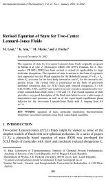
Raymond D. Mountain: Shear viscosity and dielectric constant of CH 3 CN3923TABLE II. The computed properties for the three models are listed herealong with the experimental values for the pressure, the shear viscosity, thedielectric constant and the self-diffusion coefficient. The listed uncertaintiesare described in the text.Model A Model B Model C Experiment S ,10 4 Pa•s 3.50.2 5.80.1 3.50.2 3.4 a 281 181 281 36 ap, MPa 44. 69. 6.0 0.014 bD S ,10 9 m 2 /s 3.55 2.66 3.14 4.3 ca Reference 15.b Reference 26.c Reference 27.larger than for the first method. The duration of this simulationwas 67 ps. From the slow rate of convergence indicatedin Fig. 2, this is quite likely. A sampling time an order ofmagnitude longer than 67 ps is needed for convergence ofM 2 . The estimate for reported here for Model A is consistentwith the previously reported estimates.Fixed charge models of the type examined here ignoreany induced polarization effects since the dipole moment dueto the fixed charges is quite close to the moment of the isolatedmolecule. A separate study of the Model A systemprobed the consequences of induction effects on the dielectricconstant. 24 The result is that induction would increase thedielectric constant so that the estimate would be closer to theexperimental value. A fully self-consistent simulation of inductionwas not made. This would be possible, but time consumingas such studies for other fluids has shown. 25The values of the properties for each of the models arelisted in Table II. From these simulation results, it appearsthat Model A does a slightly better job of reproducing theviscous and dielectric properties of liquid acetonitrile thandoes Model C, and both do a significantly better job thandoes Model B. Model A provides a value for the selfdiffusioncoefficient that is closer to the experimental valuethan does Model C while the reverse is true for the pressure.The value of the self-diffusion coefficient is more significantfor solution simulations than is the value of the pressuresince D S measures the mobility of the solvent. This indicatesthat the changes made in the model parameters from ModelA to Model C are not useful as they lead to a decrease in theself-diffusion coefficient. For purposes of describing a solvent,Model A is the three-site model to use in simulations.1 Y. Marcus, Introduction to Liquid State Chemistry Wiley, New York,1977, pp. 105–109.2 M. Marconelli, J. Chem. Phys. 94, 2084 1991.3 B. M. Ladanyi and R. M. Stratt, J. Phys. Chem. 99, 2502 1995.4 B. M. Ladanyi and Y. Q. Liang, J. Chem. Phys. 103, 6325 1995.5 B. M. Ladanyi and S. Klein, J. Chem. Phys. 105, 1552 1996.6 D. M. F. Edwards, P. A. Madden, and I. R. McDonald, Mol. Phys. 51,1141 1984.7 W. L. Jorgensen and J. M. Briggs, Mol. Phys. 63, 547 1988.8 J. P. Hansen and I. R. McDonald, Theory of Simple Liquids Academic,New York, 1986, p. 179.9 H. J. Bohm, I. R. McDonald, and P. A. Madden, Mol. Phys. 49, 3471983.10 S. R. Cox and D. E. Williams, J. Comput. Chem. 2, 304 1981.11 P. A. Steiner and W. Gordy, J. Mol. Spectrosc. 21, 291 1966.12 G. Del Misto and A. J. Stace, J. Chem. Phys. 99, 4656 1993.13 D. Wright and M. Samy El-Shall, J. Chem. Phys. 100, 3791 1994.14 M. W. Evans, J. Mol. Phys. 25, 149 1983.15 G. P. Cunningham, G. A. Vidulich, and R. L. Kay, J. Chem. Eng. Data 12,336 1967.16 G. J. Martyna, M. L. Klein, and M. Tuckerman, J. Chem. Phys. 97, 26351992. This paper provides a detailed discussion on the use of thermostatsin simulations.17 R. Sonnenschein. J. Comput. Phys. 59, 347 1985; D. C. Rapaport, ibid.60, 306 1985.18 M. J. L. Sangster and M. Dixon, Adv. Phys. 25, 247 1976.19 S. Nosé and M. L. Klein, Mol. Phys. 50, 1055 1983; see also, D. Brownand S. Neyertz, ibid. 84, 577 1995; J. Alejandre, D. J. Tildesley, and G.A. Chapela, J. Chem. Phys. 102, 4574 1995.20 P. Schofield, Comput. Phys. Commun. 5, 130 1976.21 S. T. Cui, P. T. Cummings, and H. D. Cochran, Mol. Phys. 88, 16571996.22 M. Neumann, O. Steinhauser, and G. S. Pawley, Mol. Phys. 52, 971984.23 M. P. Allen and D. J. Tildesley, Computer Simulation of Liquids Clarendon,Oxford, 1987, pp. 48–49.24 D. F. M. Edwards and P. A. Madden, Mol. Phys. 51, 1163 1984.25 R. D. Mountain, J. Chem. Phys. 105, 10 496 1996; addition references tosimulation studies of induced polarization are listed here.26 R. W. Gallant, Hydrocarbon Processing 48, 135 1969.27 R. L. Hurle and L. A. Woolf, J. Chem. Soc. Faraday Trans. I 78, 22331982; a slightly larger value for the self-diffusion coefficient has beenobtained from neutron scattering data, M. D. Zeidler, Ber. Bunsenges.Phys. Chem. 75, 769 1971.J. Chem. Phys., Vol. 107, No. 10, 8 September 1997Downloaded 11 Jul 2003 to 131.104.32.204. Redistribution subject to AIP license or copyright, see http://ojps.aip.org/jcpo/jcpcr.jsp