Quantitative Finance I

Quantitative Finance IModeling Volatility II(Lecture 7)Winter Semester 2013/2014 by Lukas Vacha* If viewed in .pdf format - for full functionality use Mathematica 7 notebook (.nb) version of this .pdfConditional Heteroscedastic Models - IIConditional heteroscedastic models are used for modeling s t 2 as an volatility estimate by "allowing"heteroscedasticity (time-variation) and capturing that dependence.Forecasting with GARCHEWMAGARCH-tIGARCHGARCH-MTAR-GARCHForecasting with GARCHForecasts of the GARCH can be obtained recursively2at origin h, the 1-step ahead forecast of s h+1 is:2s h+1 = a 0 + a 1 a 2 2h + b 1 s hFor multi-forecast, we use a 2 t = s 2 t e 2 2t and since EIe h+1 †F h M = 1, we have,2s h+12s h+22s h+l2= a 0 + Ha 1 + b 1 L s h2= a 0 + Ha 1 + b 1 L s h+1= a 0 + Ha 1 + b 1 L s 2 h+l , l>12s h+lØ a 01-a 1 -b 1, as lØ.Hence, the forecast converges to the unconditional variance.Exponential moving average (EWMA)Alternatively, exponential moving average (EWMA) estimator of volatility can be used. It uses all datapoints, and recent observations carry larger weights. (weights are exponentially decreasing). It also hasthe effect of diminishing the problematic “Ghost Features”.An m-period EWMA with smooth constant l is defined as:

2 QF_I_Lecture5.nbAlternatively, exponential moving average (EWMA) estimator of volatility can be used. It uses all datapoints, and recent observations carry larger weights. (weights are exponentially decreasing). It also hasthe effect of diminishing the problematic “Ghost Features”.An m-period EWMA with smooth constant l is defined as:s 2 t = ⁄ t=1ml t-1 2r t-1-t1+l+l 1 +...+l2s t+1§ tm-1where 0

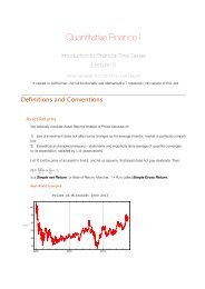
QF_I_Lecture5.nb 3Example: Real financial market data -DAX indexForecasts of variance for the DAX index. Two samples with different unconditional variance.GARCH with t innovationsAre the GARCH residuals normally distributed ? Usually the financial assets prices are fat-tailed, i.e. thedistribution has more weight in the tails then a normal distribution. In general, there is a higher probabilityof large gain (or loss) then indicated by the normal distribution.Instead of the Gaussian innovations we can use t-distributed innovations.Example: with Q-Q plotApple (AAPL) daily closing prices GARCH(1,1), Q-Q plots of residuals against the quantiles of t-distribution(tdof=6.78) and the normal distribution:

4 QF_I_Lecture5.nbApple (AAPL) daily closing prices GARCH(1,1), Q-Q plots of residuals against the quantiles of t-distribution(tdof=6.78) and the normal distribution:IGARCH - Integrated GARCHIGARCH models are unit-root (integrated) GARCH models where a 1 + b 1 = 1, their key feature is,that past squared shocks are persistent. The unconditional variance of a t is not defined under theIGARCH(1,1) model specification.The IGARCH effect might be caused by level shifts in volatility, i.e., can be spurious, (for examplelong samples. Similar to simple AR processes.) see Mikosch and Stărică (2004).IGARCH(1,1) is defined as:a t = s t e t ,s 2 2t = a 0 + b 1 s t-1where 0 < b 1 < 1+ H1 - b 1 L a 2 t-1 ,For a 0 = 0, the IGARCH(1,1) Ø infinite EWMA.Example two samples with different unconditional variance (SPX index):Sample 1: 1/02/1950 12/31/1953:s 2 2t = 0.000011 + 0.64 s t-1 + 0.14 a 2 t-1 , t-dof = 5.079.Sample 2: 1/02/2007 12/31/2010:s 2 2t = 0.0000017 + 0.9007 s t-1 + 0.09989 a 2 t-1 , t-dof = 5.651.

Sample 1: 1/02/1950 12/31/1953:s 2 2t = 0.000011 + 0.64 s t-1 + 0.14 a 2 t-1 , t-dof = 5.079.Sample 2: 1/02/2007 12/31/2010:s 2 2t = 0.0000017 + 0.9007 s t-1 + 0.09989 a 2 t-1 , t-dof = 5.651.QF_I_Lecture5.nb 5Example IGARCH(1,1) artificial processesIGARCHH1,1LSimulated seriesSimulated Volatilitya 0 0.611b 1 0.6New Random CaseExport Simulated Series80060040020000 100 200 300 400 500GARCH-M modelThe return of a security may sometimes depend directly on volatility. To model this, we use GARCH inmean (GARCH-M) model.GARCH(1,1) - M is formalized as:r t = m + cs 2 t + a ta t = s t e t ,s 2 2t = a 0 + a 1 a t-1 + b 1 s 2 t-1 ,where m and c are constant. c is also called risk premium

The return of a security may sometimes depend directly on volatility. To model this, we use GARCH inmean (GARCH-M) model.GARCH(1,1) - M is formalized as:6 QF_I_Lecture5.nbr t = m + cs 2 t + a ta t = s t e t ,s 2 2t = a 0 + a 1 a t-1 + b 1 s 2 t-1 ,where m and c are constant. c is also called risk premiumExample GARCH(1,1)-M artificial processesNote, that with positive risk premium c, returns are positively skewed, as they are positively related toits past volatilitySample GARCHH1,1L-M ACF function of a t2PACF function of a t2risk premium c -0.375a 0 0.5a 1 0.38b 1 0.318New Random CaseExport Simulated Series20-2-40 100 200 300 400 500Threshold Autoregressive (TAR)-GARCH ModelThreshold Autoregressive (TAR) model can be used to refine the model by allowing for asymmetricresponse in the (volatility) equation to the sign of shock. We can observe asymmetry in declining andrising patterns of examined time series. Model uses simple threshold to improve linear approximation.We demonstrate the idea on a simple two regime AR(1) model and then we proceed to thresholdmodel in the variance equation.

QF_I_Lecture5.nb 7Examples of Two Regime AR (1) modelTwo-Regime AR(1) model is represented by:x t =: a 1 + b 1 x t-1 + e ta 2 + b 2 x t-1 + e tx t-1 < kx t-1 ¥ kParameters are initially set to: a 1 = a 2 = 0, b 1 = -1.5 and b 2 = 0.5 to obtain following Two RegimeAR(1) process:x t =: -1.5 x t-1 + e t x t-1 < 00.5 x t-1 + e t x t-1 ¥ 0Note, that the process is stationary despite the coefficient -1.5 in the first regime. Series contains largeupward jumps when it becomes negative (due to -1.5 coefficient), and there are more positive thennegative ones. Model also contains no constant term, but E(x t L is not zero.Two Regime ARH1L modeltreshold - k 0.01a 1 0b 1 0.2a 2 0b 2 0.9New Random CaseExport Simulated Series6420-20 100 200 300 400 500ExampleSet parameters of previous example to: a 1 = a 2 = 0, b 1 = 0.2 and b 2 = 0.9 to obtain following TwoRegime AR(1) processx t =: 0.2 x t-1 + e t x t-1 < k0.9 x t-1 + e t x t-1 ¥ kand see the mixture of short-memory and long-memory processes

8 QF_I_Lecture5.nbSet parameters of previous example to: a 1 = a 2 = 0, b 1 = 0.2 and b 2 = 0.9 to obtain following TwoRegime AR(1) processx t =: 0.2 x t-1 + e t x t-1 < k0.9 x t-1 + e t x t-1 ¥ kand see the mixture of short-memory and long-memory processesExample of application: AR(1)-TAR-GARCH(1,1)TAR models can be used for capturing asymmetric response in volatility. If we find the series to followAR(1)-GARCH(1,1) process, we can introduce TAR to model asymmetric response in volatility toshocks. Model is formalized:r t = f 0 + f 1 r t-1 + a t ,a t = s t e ts 2 t = : a 220 + a 1 a t-1 + b 1 s t-122a 2 + a 3 a t-1 + b 2 s t-1a t-1 § 0a t-1 > 0

QF_I_Lecture5.nb 9ARH1L-TAR-GARCHH1,1LSimulated seriesSimulated Volatilitytreshold - k 0f 0 0.6f 1 0.5a 0 0.5a 1 0.3b 1 0.2a 2 0.5a 3 0.3b 2 0.5New Random CaseExport Simulated Series1050-50 100 200 300 400 500Empirical example TAR-GARCH(1,1)Apple (AAPL) daily closing prices sample: 9/1/2009 11/18/2011 (561 obs.)Estimated volatility eq. (normal innovations): s 2 2t = 0.00005 + 0.665 s t-1Estimated volatility eq. (t innovations): s 2 2t = 0.00004 + 0.71 s t-12+ 0.244 a t-1 IHa t-1 < 0L2+ 0.240 a t-1 IHa t-1 < 0Lwhere IHa t-1 < 0L = 1 if a t-1 < 0.Homework #4

10 QF_I_Lecture5.nbHomework #4Deadline: Tue 12.11.2013Reading: Starica, C. “Is GARCH (1, 1) as good a model as the Nobel prize accolades would imply.”Preprint (2003).https://notendur.hi.is/~helgito/NobelGarch.pdf