Orbits and Propagators - AGI

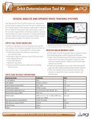
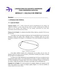
Diseño de Vehículos Espaciales 1DVE1‐T07‐3Kepler observationof Mars’ motionrelative to Earth (1609)Part I – Orbits revision

Diseño de Vehículos Espaciales 1DVE1‐T07‐5MilestonesGeocentrism (Claudio Ptolomeo, s.II aC)Heliocentrism (Nicolás Copérnico, 1543 dC)Observations (Ticho Brahe, ~1600 dC)Empirical Laws (Johannes Kepler, ~1600 dC)Analytical Laws (Isaac Newton, 1666dC)2‐body equationsof motionPLANETARYMOVEMENTBINARY STARSSPACECRAFT

Diseño de Vehículos Espaciales 1DVE1‐T07‐6Kepler’s Laws•In a 2‐body universe :‐ K‐1: The orbit of one mass aroundanother is a conic section with onebody at a focus‐ K‐2: The radius vector of the motionsweeps out equal areas in equal times‐ K‐3: The square of the period of anorbit is proportional to the cube of themean separation between the masses• Found only by observation. Newton’s laws (1643‐1727) allow toprove them

Diseño de Vehículos Espaciales 1DVE1‐T07‐7Newton’s Laws•Newton’sLaws:‐ N‐1:‐ N‐2:‐ N‐3:• Newton’s Law of Universal Gravitation:• G = 6.67x10 67x10 ‐11 Nm 2 kg ‐22r = r 2 ‐ r 1m 1F 12 F 21FFuGMm2 rrGMm u2r r / r12u21rrm 2

Diseño de Vehículos Espaciales 1DVE1‐T07‐82‐body problem2‐body equationof motionPos. of m 1 and m 2 wrt center of mass

Diseño de Vehículos Espaciales 1DVE1‐T07‐9Conservation of the specific angular momentum• Specific angular momentum of the system:• Considering polar coordinates:yrUθUrθ• Deriving the momentum:x‐ h constant and perpendicular to r‐ m 1 and m 2 confined to moving in a planeperp. to h‐ Orbit is planarKepler’s 2nd Law• Specific angular momentum:

Diseño de Vehículos Espaciales 1DVE1‐T07‐10Conservation of the specific energyElementary work made by F (exerted by P 1 on P 2 ):dW2 F dr d mv / 2GMF dr m rdW m dr mdd2mv / 2 md2vm m C2C v GM E m 2 r= potential energy per unit massConic Section Total Specific Energy (C) Major Axis aCircle 0 0)

Diseño de Vehículos Espaciales 1DVE1‐T07‐11Polar equation of the conic sections• Solve for position by integration:• Constants of integration = e, θ 0• Final result:general• Eccentricity e determines the kind of conic section:Conic SectionEccentricity (e)Circle 0Ellipse0

Diseño de Vehículos Espaciales 1Conic sectionDVE1‐T07‐122D curve, locus of points forwhich the ratio of the distancesfrom a point F and a line d isconstant and = edFd 1 d 2F 1 F 2 F 1 F 2d 2d 1d

Diseño de Vehículos Espaciales 1DVE1‐T07‐13ELLIPSEEllipse2xya bc ae212 2ba1e2θ = true anomaly. Counted from pericenter (θ =0)nE2a32a 0GMKepler’s 3rd lawAAP2a2abP1 eh2h2 P 23aP

Diseño de Vehículos Espaciales 1DVE1‐T07‐14Parabolae 1E 0vr v r( )02h22r2h1cos

DVE1‐T07‐15Diseño de Vehículos Espaciales 1Hb le 1Hyperbola02aE )1(1)(2222eaheahra1)()(1)(1)(12eareaeaercos1)(er

Diseño de Vehículos Espaciales 1DVE1‐T07‐16Exercise – Escape velocityEscape velocity is the required instantaneous velocity to ‘break’away from orbit and reach infinite distance from centre ofattraction with zero velocity.Calculate escape Δv from:(a) LEO, 200km(b) Geostationary orbit()400k (c) 400km Mars orbitYou have 5 minutes...[μ E = 4.e5 km 3 /s 2 ; R E = 6378 km; μ M = 4.2e4 km 3 /s 2 ;R M = 3396 km]

Diseño de Vehículos Espaciales 1DVE1‐T07‐17%clear all;muE = 4e5;muM = 4.2e4;RE = 6378.0;RM = 3396.0;sq2m1= sqrt(2.0)-1;% LEO h = 200 km:r = 200.0+RE; 0+RE;dv = sqrt(muE/r)*sq2m1 >> 3.23 km/s% GEO:r = 42290.0;dv = sqrt(muE/r)*sq2m1sq2m1 >> 1.27 km/s% Mars orbit h = 400.0:r = RM + 400.0; 0dv = sqrt(muM/r)*sq2m1 >> 1.38 km/s

Diseño de Vehículos Espaciales 1Orbital Elements – Making orbits usefulDVE1‐T07‐18

Diseño de Vehículos Espaciales 1DVE1‐T07‐19Orbital Elements – Making orbits useful

Diseño de Vehículos Espaciales 1DVE1‐T07‐20• Orbits are represented by a number of parameters, the most common methodis the Keplerian element set:– Inclination i• Angle between normal to orbit plane (h) and z axis;0° ≤ i ≤ 180°– Longitude of Ascending Node (RAAN in eq. coords.) Ω• angle, measured at the centre of the earth, from the vernal equinox tothe ascending node;0° ≤ Ω < 360°– Argument of perigee ω• Angle from ascending node to perigee;= angle between line of apsides and line of nodes;0° ≤ ω < 360°– Eccentricity e• Measure of how elliptical orbit is;0 ≤ e < 1; e = 0 circle– EpochT 0• Pericenter passage• Time at which this set of elements is valid

Diseño de Vehículos Espaciales 1DVE1‐T07‐21The ellipse in timeHow long does it take to go from one point to anotheron a keplerian orbit?Mean anomaly M = fraction of an orbit period which has elapsedsince pericenter, expressed as an angle:DEF: M‐ M o = n(t‐t 0 ) with M o = M (t=t 0 )n = 2π/PThe link between M and θ is theeccentric anomaly E2e cos1e sincos E ; sin E 1ecos1ecos....a bit of geometry algebra give :M E esinEM M0 n(t t0)t t ( MM) 0 /n0

Diseño de Vehículos Espaciales 1DVE1‐T07‐22TLEs (Two Line Elements Sets)• A standard text format for sharing orbit information• Updated and distributed regularly by NASA GSFC[http://celestrak.com/NORAD/elements/]1 AAAAAU YYLLLPPP BBBBB.BBBBBBBB .CCCCCCCC DDDDD-D EEEEE-E F GGGGZ2 AAAAA HHH.HHHH HHHH III.IIII IIII JJJJJJJ KKK.KKKK KKKK MMM.MMMM MMMM NN.NNNNNNNNRRRRRZNNNNNNNNRRRRRZ• Example TLE for the International Space Station:SOYUZ-TMA 131 33399U 08050A 08291.52340378 .00013791 00000-0 10622-3 0 1562 33399 51.6416 109.1653 0003546 229.8945 178.2709 15.72317173567788

Diseño de Vehículos Espaciales 1DVE1‐T07‐23TLEs – Line 11 AAAAAU YYLLLPPP BBBBB.BBBBBBBB .CCCCCCCC DDDDD-D EEEEE-E F GGGGZ• [1] ‐ Line #1 label• [AAAAA] ‐ Catalogue number• [U] ‐ Security Classification• U = Unclassified• C = Classified• S = Secret• [YYLLLPPP] ‐ International Designator• YY = 2‐digit Launch Year• LLL = 3‐digit Launch day of the Year• PPP = up to 3 letter Sequential Piece IDfor launch• [BBBBB.BBBBBBBB] ‐ Epoch Time• 2‐digit year, 3‐digit day of the year• time represented as a fraction of 1 day•[.CCCCCCCC] ‐ Drag Parameter (rev/day 2 )• 0.5 x dN/dt

Diseño de Vehículos Espaciales 1DVE1‐T07‐24TLEs – Line 1 ctd1 AAAAAU YYLLLPPP BBBBB.BBBBBBBB .CCCCCCCC DDDDD-D EEEEE-E F GGGGZ• [DDDDD‐D] ‐ Drag Parameter (rev/day 3 )• 1/6 x d 2 N/dt 2•"‐D" is the tens exponent (10‐D).• [EEEEE‐E] E] – B* Drag Parameter (1/Earth Radii)B * = C D ρ 0 A / 2m• Pseudo Ballistic Coefficient• The "‐E" is the tens exponent (10‐E)• [F] ‐ Ephemeris Type• 1‐digit integer (0 = SGP or SGP4)• [GGGG] ‐ Element Set Numberassigned sequentially• [Z] ‐ Checksum (1‐digit integer)• Computed from sum of all integercharacters plus 1 for each “‐”• Modulo‐10 of the result is ‘Z’ oneach line

Diseño de Vehículos Espaciales 1DVE1‐T07‐25TLEs – Line 22 AAAAA HHH.HHHH III.IIII JJJJJJJ KKK.KKKK MMM.MMMM NN.NNNNNNNNRRRRRZ• [HHH.HHHH] ‐ Orbital Inclination ‐ [0, 180]• [III.IIII] ‐ Right Ascension of the Ascending Node ‐ [0, 360]• [JJJJJJJ] ‐ Orbital Eccentricity• implied leading decimal point ‐ [0.0, 1.0)• [KKK.KKKK] ‐ Argument of Perigee ‐ [0, 360]• [MMM.MMMM] ‐ Mean Anomaly ‐ [0, 360]• [NN.NNNNNNNN] ‐ Mean Motion (revolutions per day)• [RRRRR] ‐ Revolution number

Diseño de Vehículos Espaciales 1DVE1‐T07‐26Inclination regimesand also by inclination i …i = 0° i = 90°EquatorialPolar0° ≤ i < 90°Posigrade,Direct,Prograde90° < i ≤ 180°Rt Retrograde,Indirect

Diseño de Vehículos Espaciales 1DVE1‐T07‐27Ground Tracks• Application orbits are determined by the users’ desired groundtrack• Ground track is the path the sub‐satellite point traces over theEarth’s surface during its orbit

Diseño de Vehículos Espaciales 1DVE1‐T07‐28Ground TracksEquatorialorbitHST orbit (i=28.5 deg)GeosynchronousGeosynchronous

Diseño de Vehículos Espaciales 1DVE1‐T07‐29Earth‐synchronous orbits• Orbit whose period is contained an integer number of times inone Earth rotation. Therefore, the ground track closes onto itself.• Examples:– Geosynchronous (P=24h), semi‐synchronous (P=12h)–P = 4 h, P = 2 h, P = 6 h

Diseño de Vehículos Espaciales 1DVE1‐T07‐30The real Universe is not so simple• There are many more forces acting on a spacecraft than just a single gravitypull of e.g. Earth the 2‐body equations are solvable, but useless for realmission design.• We can make the model more realistic (and harder to solve) in 2 main ways:– Add more gravity sources– Add other forces• Solving a general n‐body problem is analytically difficult, and in generalcontains 6n parameters for which we do not have sufficient independentintegrals.• For spacecraft, we can simplify the n‐body problem to the restricted 3‐bodyproblem, by setting the mass of the 3rd body (spacecraft) to be negligiblecompared to other 2 masses (e.g. Earth, 610 24 kg, and Moon, 710 22 kg)

Diseño de Vehículos Espaciales 1DVE1‐T07‐31Perturbations• So far, we consider gravity to be a field that behaves in a purely 1/r sphericalway• It should be obvious that the Earth is not spherical, and even if it was, there isno reason why the gravity field should be spherical.Gravity Map of Earth;Credit: JPL, NASA

Diseño de Vehículos Espaciales 1DVE1‐T07‐32Perturbations overview• No closed‐form analytic solution –also time‐varying (e.g. with solar cycle)• For design, instead take average values or guidelines – this will be a key lessonfor many subsystems!Source Acceleration (ms ‐2 )@500km@GEOAtmospheric Drag 6 x 10 ‐5 A/M 1.8 x 10 ‐13 A/MRadiation Pressure 4.7 x 10 ‐6 6A/M 4.7 x 10 ‐6 6A/MSun (mean) 5.6 x 10 ‐7 3.5 x 10 ‐6Moon (mean) 12x 1.2 10 ‐6 73x 7.3 10 ‐6Jupiter (mean) 8.5 x 10 ‐12 5.2 x 10 ‐11A = projected area; M = mass

Diseño de Vehículos Espaciales 1DVE1‐T07‐33Perturbations overview

Diseño de Vehículos Espaciales 1DVE1‐T07‐34UNon‐spherical gravity• An representation in spherical harmonics is used to define a general gravityfield of a massive body:nn n RE REr, ,1 JnPn, 0cos Cn,mcos m Sn,msin m Pn, mcos rn2 rm1r • J, S and C are dependant upon the mass distribution of the central body, and are latitude and longitude, and P n,m are Associate Legendre Functions.J2 dominates by FAR

Diseño de Vehículos Espaciales 1DVE1‐T07‐35Regression of Line of Nodes• The bulge produces a torque that rotates the angular momentum vector. Forprograde (i < 90°), theorbit itself rotates tt to thewest. t• Ifweignore everything except J 2 , the regression is approximated as: Jn 20 t tO[J]3 RE nJ22 a3aJ202cosi22 1 e 2= mean motion

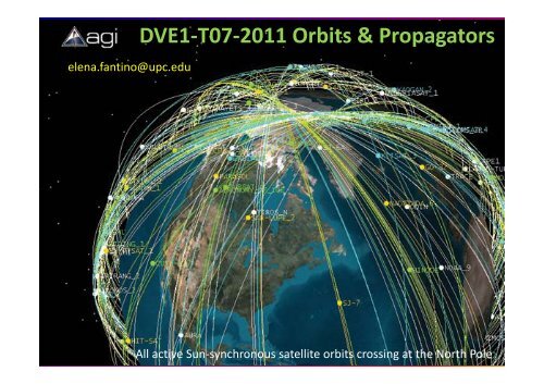
Diseño de Vehículos Espaciales 1DVE1‐T07‐36Sun‐synchronous orbits• LEO orbits whose line of nodes precesses (eastward, henceretrograde orbit) so as to mach the apparent angular motion ofthe Sun around the Earth o0.9856/day

Diseño de Vehículos Espaciales 1DVE1‐T07‐37Precession of Line of Apsides• If you are sitting in your spacecraft, as you cross the plane of the equator, you‘feel’ more mass than the mean value• Your orbit curves more rapidly (faster fall)• Conservation of energy leads to a rotation of the orbit within the plane• Thiscan only happen if the major axis rotates, so the line of apsides (joiningperigee and apogee) must rotate. J03nJ4J2t t R a0 O[J2E212]22 4 5sini1e22• For i = 63.4°, = 0. This means that apogee for orbit at this inclinationalways stays in the same place over the Earth. This was discovered by theSoviet Union in 1960s, and the Molniya orbit was invented.

Diseño de Vehículos Espaciales 1DVE1‐T07‐38Molniya orbitApprox 12h period, very highelliptical orbitFirst successful launch: Aug 1965.Semi‐synchronous orbit

Diseño de Vehículos Espaciales 1DVE1‐T07‐39Atmospheric Drag• For low‐orbit spacecraft, the very thin edge of the atmosphere creates dragand lift forces, as it would for any flying object. We are going to ignore lift.FD1 SC2 DV2r VVrr• C D is hard to estimate; there is a large mean free path, so free molecular flowis most suitable model (no shock wave, no particle interactions). Typicalvalues are around C D = 2,5.• S is usually taken as the cross‐sectionalsectional area projected in the direction of thevelocity vector.• By inspection, drag will reach a peak at perigee, because both velocity anddensity are at their maximum values. Intuitively, the drag force can beconsidered a negative, impulsive velocity increment at perigee.• For an ellipse, this reduces the semi‐major axis; for a circular orbit, dragoccurs continuously and reduces the radius.

Diseño de Vehículos Espaciales 1DVE1‐T07‐40Solar Radiation Pressure (SRP)• Incident radiation from the Sun imparts momentum to illuminated objects.• Reflecting light from a surface represents a momentum exchange. There istherefore a small, but measurable, ‘pressure’ effect: P Fc• F * is the solar energy flux at the spacecraft, c is speed of light.• At Earth orbit, F * = 1400Wm ‐2 so solar radiation pressure is aboutP = 4.710 ‐6 Nm ‐2• This is very small, but the effect it has depends on the surfaces of the spacevehicle.• The perturbing effect of the SRP depends upon the area‐to‐mass ratio A/m,and is inversely proportional to the square of the distance from the Sun.• The size of the force per unit spacecraft mass (the perturbation), is empiricallyassembled:2( A a f 1) SRPkrPm r• Kr is a parameter representing ‘reflectivity properties’: k r = 0.0 for fullabsorption, k r = 0.4 for diffuse reflection, k r = 1.0 for specular reflection

Diseño de Vehículos Espaciales 1DVE1‐T07‐41One‐impulse maneuversConsist in applying an impulse at some point (r 1 ,θ 1 ) of the orbitcharacterized by velocity and flight path angle (v 1 ,γ 1 ).The result is a new orbit with true anomaly θ 2 and velocity andflight path angle (v 2 ,γγ 2 ). The radius vector r 1 does notchange: the point of application of the maneuver does not change,the velocity does.Final orbitΔVV 1V 2LocalhorizonFlight path angle γ = angle from localhorizon to velocity vectorInitial orbit

Diseño de Vehículos Espaciales 1DVE1‐T07‐42Two‐impulse maneuvers: Hohmannv Initial velocity (r 1 )vv12rr1r2Final velocity (r 2 ) r1r r2a r rr re 2 r r2 rrr r r 2vrr 3 T arv1v v12r2r r r r1 21 1v2v2 vr22rr r 2r211

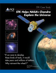
Diseño de Vehículos Espaciales 1Part II ‐ PropagatorsDVE1‐T07‐43

Diseño de Vehículos Espaciales 1DVE1‐T07‐44Why do orbits matter for design?• Orbit size determines period; they both determine lighting levels anddirections…• Lighting determines potentially available solar power…• Distance from Sun determines direct thermal load; distance from Earth orother body determines indirect IR and albedo lighting and heating…• Night‐side id flight and eclipses determine dt worst‐case thermal rates…• Geometry of nodes and inclination determines visibility and duration ofoverflights for communications…• Overflight duration determines required memory size, on‐board processingpower, and communications constraints…

Diseño de Vehículos Espaciales 1DVE1‐T07‐45Why do orbits matter for design?• Communication constraints determine the frequency, coding, and modulationof link…• Communication link design drives power requirement for amplifiers andantennas…• Power requirement drives solar array size…• Solar array size di drives attitudecontrol requirements…• Rate requirements place limits on thruster/actuator size, which determinesfuel requirement, which sizes the structures…• and so on…

Diseño de Vehículos Espaciales 1DVE1‐T07‐46Introduction to propagators• Predicting the orbits of satellites is an essential part of mission analysis andhas impacts on the power system, attitude control and thermal design.• It is the starting point in planning whether a proposed mission is feasible andhow the satellite(s) need to be designed.• The computation of the orbits of artificial satellites around planets such as theEarth has been studied in detail in the last century.• The problem of computing the orbits of satellites, however, is notstraightforward. The main factors affecting the orbit of a satellite are:– the non‐spherical Earth,– atmospheric drag,– perturbative effects from the gravitational pull of the Sun and otherplanets– radiation pressure.

Diseño de Vehículos Espaciales 1DVE1‐T07‐47Introduction to propagatorsThese effects are important in different levels for different types of satelliteorbits. For example satellites in LEO are strongly affected by the nonsphericalnature of the Earth and even atmospheric drag. Satellites out ingeostationary orbit, however, are sufficiently far from the Earth for theseeffects to be ignorable. The gravitational pull of the Sun and Moon, however,does play a significant role in the evolution of their orbits. Effects such asatmospheric drag and radiation pressure are also very dependent upon theshape, size and mass of the satellite.

Diseño de Vehículos Espaciales 1DVE1‐T07‐48Propagators• The purpose of satellite orbit propagators is to provide high accuracy inpredicting the position of a satellite.• Orbits are simulated numerically for future time steps to predict where asatellite/vehicle will be in the future (necessary in order to plancommunications, manage operations, etc.)• Analytical solutions apply a time‐limited rule about how position and velocitywill change in a small time step, and apply them to the previous state• Starting from a set of initial conditions at t=0, the evolution of an orbit ispropagated into the future• In order to achieve precision, a very short time step is required. However, thecalculation of the forces acting on a satellite at each time step slows down thecomputation which makes it prohibitive to propagate anything but crudeforce models on the satellite itself.• This means that it is important to identify the forces that mainly affect a givenorbit in order to propagate an adequate and appropriate it force model dlandavoid spending computing time with complete and detailed force models.

Diseño de Vehículos Espaciales 1DVE1‐T07‐492‐body propagators• 2‐body propagator assumptions:– satellites travel high enough above the atmosphere so that the drag forceis small– the satellite won’t perform manoeuvres (we can ignore any thrust)– we only consider the motion of the satellite close to the Earth– we can ignore the gravity of the Sun, the Moon or anything else– compared to Earth’s gravity, other forces e.g. solar radiation pressure,electromagnetic fields, etc. are negligible– the mass of the Earth is much, much larger than the mass of thespacecraft– the Earth is spherically symmetrical with uniform density (so assume it is apoint mass)• A 2‐body propagator does not need numerical integration in a forcemodel. The model allows for closed‐form solution, with the only need fora numerical technique to solve Kepler’s equation

Diseño de Vehículos Espaciales 1DVE1‐T07‐50Kepler’s equation with NR% From time to true anomaly with the solution of Kepler's equation byNewton-Raphsonclear all;% constantstwopi = pi + pi;% data:e = 0.4; % eccentricityt0 = 0; % epoch of pericenter passageP = 5800.0; % period (sec)t = 35.0; % time (min)tol = 1.e-10;% from min to sect = t*60.0;% mean motionn = twopi/5800.0;% mean anomaly at tM = n*(t-t0);

Diseño de Vehículos Espaciales 1DVE1‐T07‐51% NR loopdE = 1.0;E = M % first guess for Eiter = 0; % iteration counterwhile(dE > tol)iter = iter + 1;Eold = E;E = E + (M+e*sin(E) - E)/(1.0-e*cos(E));dE = abs(Eold-E);enditer >> 4E*180/pi >> 143.9 deg% from E to true anomaly:cE = cos(E);sE = sin(E);cth = (e-cE)/(e*cE-1.0);sth = sqrt(1.0-e*e)*sE/(1.0-e*cE);th = atan2(sth,cth)*180/pi % true anomaly (deg) >> 155.9 deg

Diseño de Vehículos Espaciales 1DVE1‐T07‐52Propagators• However, propagators can include terms that correct for some of the modelassumptions and hence introduce some additional force.• This requires propagation equations (either analytical or numerical)• We will not be concerned with deriving the propagation equations, but willlearn about the main propagators and their differences[New geometric integration schemes have been developed recently which exploitthe geometric properties of the orbital dynamics of a satellite. These are calledsymplectic methods. Explicit schemes have been developed which also enablevery fast computation of the satellite orbit for a given required level of accuracy.As well as the accuracy, symplectic schemes also provide a method for splittingtime steps for different types of force, and this can be exploited for satellites togreat effect, greatly reducing the expensive force calculations. The resultingpropagation schemes are now able to compute accurate orbit trajectoriesonboard the satellite and therefore enable real time accurate orbit determin.]

Diseño de Vehículos Espaciales 1DVE1‐T07‐53STK Propagators• When using STK to get useful engineering values, remember to choose asuitable propagator.• STK uses 2 basic types: numerical and analyticalAnalytical propagators use a closed‐form solution of the time‐dependentmotion of a satellite to produce ephemeris or to provide directly the positionand velocity of a satellite at a particular time.Numerical propagators numerically integrate t the equations of motion for thesatellite.http://www.stk.com/resources/help/online/stk/source/stk/vehsat_orbitprop_choose.htm

Diseño de Vehículos Espaciales 1DVE1‐T07‐54STK Propagators• Main propagators to use are:– J 2 Perturbation (1st Order) LEO•The J 2 Perturbation (first‐order) propagator accounts for variations inthe orbital elements due to Earth oblateness.•Does not model atmospheric drag•Does not model solar or lunar gravity– J 4 Perturbation (2nd Order) LEO•The J 4 propagator includes the 1st & 2 nd order effects of J 2• Includes the 1st order effects of J 4•J 4 is approximately 1000 times smaller than J 2• Little difference between orbits propagated with J 2 and J 4

Diseño de Vehículos Espaciales 1DVE1‐T07‐55STK Propagators– HPOP(High Precision Orbit Propagator)• HPOP can handle orbits up to and beyond the Moon• Includes 1st order effects of J 4– SGP4 LEO, GEO, HEO• Simplified General Perturbations (SGP4) propagator is used with TLEs• Includes J 2 and J 4•Also includes Solar and Lunar gravity and gravitational resonance• Includes orbit decay using a simple drag model– LOP•Long‐term (months, years) propagator– Astrogator• Includes thrusts, manoeuvres, and targeting

Diseño de Vehículos Espaciales 1DVE1‐T07‐56STK Propagators– StkExternal propagator: allows to read the ephemeris for a satellite from afile. The file must end in an .e extension.– SPICE: reads ephemeris from binary files that are in a standard formatproduced by the Jet Propulsion Laboratory (JPL). They are intended forephemeris for celestial bodies but can be used for spacecraft (seeinstruction in STK page)– Real‐time: allows to propagate vehicle (all types) ephemeris using nearreal‐timedata received using a connect socket

Diseño de Vehículos Espaciales 1DVE1‐T07‐57STK Propagator summaryEarthSun LunarJ2 J4GravityGravityGravitySolarWindOtherPlanetsEarthAtmos’Thrusts2‐BodyJ2J4SGP4 (TLE)HPOPAstro‐gatorLOPThe remaining i three (StkExternal, SPICE and Real‐time) are based onEphemerides (they do not use models), hence they do not appear in thetable

Diseño de Vehículos Espaciales 1Part III - STK BasicsDVE1‐T07‐58

Diseño de Vehículos Espaciales 1DVE1‐T07‐59What is STK?• STK is a physics‐based software geometry engine that accurately displays andanalyzes land, sea, air, and space assets in real or simulated dtime.• Users can model the time‐dynamic position and orientation of vehicles viavarious propagation p algorithms or external inputs.• Given these dynamic positions and orientations, users can model thecharacteristics and pointing of– Sensors– Communications– Other payloads aboard the asset.• STK can then determine spatial relationships (e.g. line of sight) between anasset of interest and all of the objects under consideration.• STK's technically‐accurate 2D and 3D visualization and analytical data outputscan help enhance situational awareness and understanding.• Users can share their results with others via snapshots, movies, and even VDFfiles for use in AGI Viewer.

Diseño de Vehículos Espaciales 1DVE1‐T07‐60Creating tutorial scenario• Open STK, close the Launchpad• File → New

Diseño de Vehículos Espaciales 1DVE1‐T07‐61General configuration• Edit→ Preferences→ Save/Load Prefs– verify that Save Vehicle Ephemeris is enabled and Binary Formatis disabled– verify that Save Accesses is disabled– verify that Auto Save is enabled, and that the Directory field ispopulated with the location where you want to save STK files.Set the Save Period to 5 min (300 sec)• Object Browser:– Select the scenario, right‐click, open the Properties browser– Basic properes → Time Period →•Start: 6 Oct 2011 8:00• Start: 6 Oct 2009 14:00→ [Apply]

Diseño de Vehículos Espaciales 1DVE1‐T07‐62Scenario configuration• Check the start time on the ‘animation’ settings page also→ [OK]• Select 2D map view, and edit properties• Select Overlays. In the Animation Time frame, turn on the Showoption, set X to 20 and Y to –20, set Text Color to white• Disable the background• In Details page, remove International Borders from the selectedlist, and disable Lt/L Lat/Lon lines ‘Show’ (i.e. hide them)• Disable background image, and set color to black• In Projection page, verify that the Type is set to EquidistantCylindrical, and check Center Lon is 90 deg.

Diseño de Vehículos Espaciales 1DVE1‐T07‐63Initialise 2D display• Open the Map Annotaons page → [Add…]• Enter your name as ‘String’, set Position Type to X,Y• Set X = ‐160, Y = ‐60→ [OK]• Reset theanimationreset

Diseño de Vehículos Espaciales 1DVE1‐T07‐64Configuring the scenario• In Object Browser, rename the scenario to DVE1 (right‐click)• ‘Right menu’ also provides linksto many features of the tools• Add a satellite:Insert → New…• Satellite→ [Insert]• Canceltheorbit wizard

Diseño de Vehículos Espaciales 1DVE1‐T07‐65Configure the satellite• Maximise the 2D map view• Rename the satellite to ‘Molniya’ (right‐click → Rename)• Molniya → Right‐click → Properes → Basic → Orbit• Set:–Propagator → TwoBody– Semi‐major major axis → 26554 km– Eccentricity → 0.72– Inclinaon→ 63.14°–Argument of Perigee → 270°– RAAN → 0°–Orbit Epoch: 1 Jul 2007 00:00:00.000 UTCG→ [OK]• Reset the animation, i then play it

Diseño de Vehículos Espaciales 1DVE1‐T07‐66Creating a ground station• Select the DVE1 scenario• Insert → New…Facility → [Insert]• Rename the facility to ‘Terrassa’• Open the properties browser, and set:– Latitude: 41:33:45.2700 DMS– Longitude: 02:01:24.7500 DMS– Select ‘Use Terrain Data’– Local time offset from GMT: 7200 sec→ [OK]

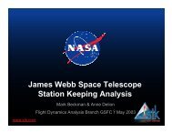
Diseño de Vehículos Espaciales 1DVE1‐T07‐67Add another satellite• Select the DVE1 scenario• Insert → Satellite from database• Select ‘Common Name’ → ISS• Select SSC=25544 → [OK]• Reset, start simulation, and explore the map views and settings

Diseño de Vehículos Espaciales 1DVE1‐T07‐68

Diseño de Vehículos Espaciales 1DVE1‐T07‐69Calculate access (times)• Select Terrassa in the scenario• Right click → Access• Select ISS (leave other sengs) → [Compute]• Reports panel → [Access]

Diseño de Vehículos Espaciales 1DVE1‐T07‐70Calculate Access (AER)• → [AER] (Azimuth, Elevaon, Range)

Diseño de Vehículos Espaciales 1DVE1‐T07‐71Graphing Results

Diseño de Vehículos Espaciales 1DVE1‐T07‐72Using sensors• Remove the ISS from the scenario• Add a sensor to Molniya:– Select Molniya–Insert → New… → Sensor–rename the sensor ‘horizon’• Open sensor properties:– Definition: Simple conic, cone angle = 90°–Pointing: Fixed, elevation = 90°→ [OK]• Reset and run the scenario• Change the cone angle to 45°, 25°, 5° and re‐run the scenario• Adjust 3D options of the sensor display

Diseño de Vehículos Espaciales 1DVE1‐T07‐73Using sensors• Add a sensor to Terrassa:–Name = ETSEIAT–Sensor Type = Complex Conic– Inner Half Angle = 0°–Outer Half Angle = 85°– Minimum Clock Angle = 0°– Maximum Clock Angle = 360°–Pointing = Fixed–Elevation = 90°• ETSEIAT → 2D graphics projecon properes → projecon–Extension distances → maximum altude = 785–Project to: constant altitude, step count = 1

Diseño de Vehículos Espaciales 1DVE1‐T07‐74Using sensors• Reset and run the scenario• Ground sensor projects a fixed region of ‘possible reach’projected onto the map, up to a fixed altitude

Diseño de Vehículos Espaciales 1DVE1‐T07‐75STK Training• Repeat this scenario for yourself• In STK → Help → Desktop Applicaon Help → Tutorials– Introducing STK– 3D graphics• Objective: get familiar with the tool, with the way to setparameters, add objects, visualise results.• STK will be used in later topics, as a ‘simulation engine’ that givesresults about: lighting, thermal, communications conditions… etc.• It is important that you become happy with it. It is powerfuland rather easy to use.

Diseño de Vehículos Espaciales 1DVE1‐T07‐76Some ready‐to‐use scenarios• sim‐geo.vdf• ExampleOrbits.vdf• sim‐hohmann‐transfer.vdf• DVE1_STK_Examples.vdf

Diseño de Vehículos Espaciales 1DVE1‐T07‐77To be included in the report of “Proyecto de Equipo – parte 1”:• First of all: download & install software, apply for licence and install it• Follow installation instructions available in Atenea• Very few people have completed this step, the rest are “warmly” invited toproceed...THEN:• Take your study satellite and create a scenario for its orbit, and one groundstation (or all if it has more than one and you feel like it).• Set the time frame for your scenario• Change any display parameters• Run the scenario and obtain:– A 2D ground track plot– An access report for the ground station‐to‐satellite(if you have many accesses –give only max, min, mean values)• It is not a bad idea (and will cause you no harm) that of the threemembers of each group each performs the exercise independently andthen exchanges and discusses results with the group...