Introducing_a_relative-value_tool_for_swaps_19_08_13_08_57

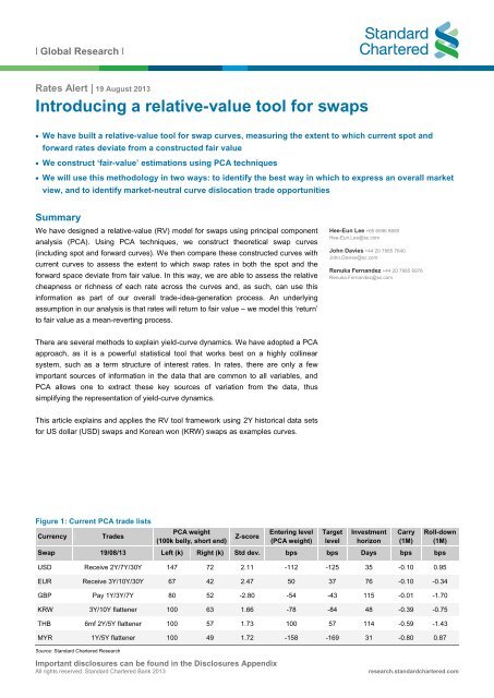
l Global Research lRates Alert | 19 August 2013Introducing a relative-value tool for swaps We have built a relative-value tool for swap curves, measuring the extent to which current spot andforward rates deviate from a constructed fair value We construct ‘fair-value’ estimations using PCA techniques We will use this methodology in two ways: to identify the best way in which to express an overall marketview, and to identify market-neutral curve dislocation trade opportunitiesSummaryWe have designed a relative-value (RV) model for swaps using principal componentanalysis (PCA). Using PCA techniques, we construct theoretical swap curves(including spot and forward curves). We then compare these constructed curves withcurrent curves to assess the extent to which swap rates in both the spot and theforward space deviate from fair value. In this way, we are able to assess the relativecheapness or richness of each rate across the curves and, as such, can use thisinformation as part of our overall trade-idea-generation process. An underlyingassumption in our analysis is that rates will return to fair value – we model this ‘return’to fair value as a mean-reverting process.Hee-Eun Lee +65 6596 8690Hee-Eun.Lee@sc.comJohn Davies +44 20 7885 7640John.Davies@sc.comRenuka Fernandez +44 20 7885 6976Renuka.Fernandez@sc.comThere are several methods to explain yield-curve dynamics. We have adopted a PCAapproach, as it is a powerful statistical tool that works best on a highly collinearsystem, such as a term structure of interest rates. In rates, there are only a fewimportant sources of information in the data that are common to all variables, andPCA allows one to extract these key sources of variation from the data, thussimplifying the representation of yield-curve dynamics.This article explains and applies the RV tool framework using 2Y historical data setsfor US dollar (USD) swaps and Korean won (KRW) swaps as examples curves.Figure 1: Current PCA trade listsCurrencyTradesPCA weight(100k belly, short end)Z-scoreEntering level(PCA weight)TargetlevelInvestmenthorizonCarry(1M)Roll-down(1M)Swap 19/08/13 Left (k) Right (k) Std dev. bps bps Days bps bpsUSD Receive 2Y/7Y/30Y 147 72 2.11 -112 -125 35 -0.10 0.95EUR Receive 3Y/10Y/30Y 67 42 2.47 50 37 76 -0.10 -0.34GBP Pay 1Y/3Y/7Y 80 52 -2.80 -54 -43 115 -0.01 -1.70KRW 3Y/10Y flattener 100 63 1.66 -78 -84 48 -0.39 -0.75THB 6mf 2Y/5Y flattener 100 57 1.73 100 57 114 -0.59 -1.43MYR 1Y/5Y flattener 100 49 1.72 -158 -169 31 -0.80 0.87Source: Standard Chartered ResearchImportant disclosures can be found in the Disclosures AppendixAll rights reserved. Standard Chartered Bank 2013research.standardchartered.com

FlyRates AlertThe benefits of adopting a PCA approachIn order to increase and improve the flow of our trade recommendations in the swapspace, we have built an RV tool using PCA. This methodology allows us to generatefair-value swap curves in both the spot and forward space based on just a few (inthis instance, three) key explanatory risk factors – the principal components.Typically in rates, the most important risk factors are parallel shifts, changes in slopeand changes in convexity of the curve. We find that the first three principalcomponents capture over 99% of the variation in the curves, and as such justify thechoice of only the first three principal components in the construction of fair-valuecurves. Given a fair-value curve, we can compare it with the current market curve toidentify RV opportunities.We have applied this methodology not only to G10 rates markets but also to theemerging-market (EM) rates markets that we cover. Using a two-stage approach, wefirst identify rich/cheap points on a given swap curve. As a second step, the RV tooluses the identified cheap/rich points to structure directionally neutral curve andcurvature trades, such as butterflies. In this way the tool can also be used to assesswhether a particular trade is indeed exposed to the curve in the way one would expect.For example, the tool can verify whether a given butterfly trade is actually exposed tochanges in the convexity of the curve or mainly to slope and level changes.For every trade our tool generates, it will provide a visualisation package of importantanalytics and graphics covering factors such as PCA weights, carry, roll-down, targetprofit and investment horizon. This visualisation package allows the characteristics ofthe trade to be captured in a more user-friendly way. The RV tool will form part of ourframework for identifying and valuing trade opportunities in swap curves. In ratesresearch, we will update our preferred trade ideas as and when identified by our RVtool. Eventually, we intend to roll out the complete package to our clients, and we willbe happy to provide support and advice on the results generated whenever required.We provide the mathematical details of the technical aspects of our PCA toolmethodology in the Appendix.Figure 2: US curve directionality increased after thefinancial crisis5Y swap rates, 2Y/10Y curve and 2Y/5Y/10Y butterfly8.07.06.05Y outright5.04.03.02Y/5Y/10Y2.02Y/10Y1.00.0-1.0May-01 May-03 May-05 May-07 May-09 May-11 May-13Source: Standard Chartered ResearchFigure 3: No directionality in PCA tradesPCA weighted USD 2Y/5Y/10 butterfly vs. the 5Y level2.0%1.8%1.6%1.4%1.2%1.0%0.8%0.6%0.4%Level vs. Fly0.2%0.0%-0.6% -0.6% -0.5% -0.5% -0.4%LevelSource: Standard Chartered Research19 August 2013 2

Rates AlertThe PCA database is taken fromtrader-sourced closing levelsPCA framework – Building blocks for RV tradesStep 1 – DatabaseWe use swap data taken from historical trader-sourced closing levels. Our tradeidentification is based two years of historical data, as it represents the curve’smovement within a reasonable volatility range and the larger part of the investmenthorizon is within two years. However, the sample period used may be varied.Forward curves for each market are derived from the spot curve using existing inhousequant functionality.Three principal components capturethe majority of the yieldcurvedynamicsStep 2 – Three principal componentsPCA allows us to reduce a covariance matrix of our set of interest rates into animportance-ordered subset of uncorrelated variables, i.e., the principal components(PCs). More simply, it allows us to express each rate as a linear combination of just afew (in this instance, three) variables – the PCs. The total number of PCs is equal tothe number of observed variables. In our case, the observed variables are time seriesof interest rates of various maturities. The number of PCs used to express each ratedepends on how much variance one wants to explain. Using all the components willexplain all the variation in the observed variable; however, one may choose to usefewer PCs, as some of the minor variations may be viewed as noise.The analysis explicitly reveals the importance of each PC (its factor), which is anexpression of the contribution of that component to the variables in question, i.e., in thiscase to interest rates. Also associated with each PC is a set of ‘factor loadings’ thatdefine how each rate will change (by how much and in what direction) to a shock to thatcomponent.In interest rates, it is typical for the first three PCs to capture over 95% of thevariation in the curve. As such, we choose to express each rate as a combination ofthe first three components.We perform the PCA on the spot curve and forward curves separately. We thenestimate the current fair value of each interest rate along a given curve using the firstthree PCs that are distinct to that curve. For example, the 1Y rate would beexpressed as a linear combination of three PCs where those PCs are distinct to thespot curve. Similarly, the 1Y/1Y rate would be expressed as a linear combination ofFigure 4: Historical PCA12%10%8%Historical PC1 vs. US 10Y Historical PC2 vs. US 5Y/30Y curve Historical PC3 vs. US 5Y/10Y/30Y butterflyPC1(LHS)4%3%2%1%5Y-30Ycurve(RHS)3%2%1.3%1.1%PC3(LHS)0.5%0.3%6%2%0.1%4%2%10Y level(RHS)1%0%PC2(LHS)1%0.9%5Y/10Y/30Ybutterfly(RHS)-0.1%0%Apr-11 Oct-11 Apr-12 Oct-12 Apr-130%-1%Apr-11 Oct-11 Apr-12 Oct-12 Apr-130%0.7%Oct-11 Apr-12 Oct-12 Apr-13-0.3%Source: Standard Chartered Research19 August 2013 3

Rates Alertthe three PCs that are distinct to the 1Y forward curve. The result is that each rate isexpressed as a linear combination of three PCs. As such, the time series of yieldcurve data is transformed into the time series of combinations of three PCs.PC1 can be considered a measureof the outright levelInterpretation of the principal components:PC1 – LevelIn a perfectly correlated system of changes in interest rates or levels in interest rates,the factor loadings of the first principal component would be equal. More generally,the more correlated the system, the more similar the values of the loadings of the firstprincipal component across the variables. As such, the first principal componentcaptures a ‘common trend’ in the variables. So, if the first principal componentchanges and the other components remain fixed, then the variables in your system,in this case the interest rates, will all move by roughly the same amount. As such, inrates space, PC1 can be considered a measure of the outright ‘level’ of yields.PC2 is the proxy for the slope ofthe curvePC2 – SlopeIf the system of variables has no natural order, then the second and higher-orderprincipal components may have no intuitive interpretation. However, with interest rates,the system is ordered, i.e., there are set rates of various maturities. The loadings of thesecond principal component typically decrease (or increase) in magnitude with maturity.As such, if PC2 changes while the other components remain the same, then the ratesat one end of the term structure will move up and the others will move down. For thisreason, PC2 can be considered a proxy to the slope of the curve.PC3 represents the curvature ofthe curvePC3 – CurvatureSimilarly for PC3, the loadings of PC3 typically decrease (or increase) in magnitudeand then increase (or decrease). As such, if PC3 changes while the othercomponents remain constant, then the rates at either end of the term structure willmove up, and the rates in the middle will move down.As mentioned above, each principal component has an associated factor thatrepresents the importance of this principal component in capturing the variation in theFigure 5: The three PCs and the loading vectorSource: Standard Chartered ResearchFigure 6: PC1, PC2 and PC3 explain 99% of the curveThree PC loadings for the US swap curveFigure 7: PC – Explanation level for yield-curve variance0.70.60.50.40.30.20.10.0-0.1-0.2-0.3-0.4PC1PC3PC21Y 2Y 3Y 4Y 5Y 7Y 8Y 9Y 10Y 15Y 20Y 25Y 30Y 40Y100%80%60%40%20%0%PC1 PC2 PC3MYR HKD KRW EUR USD JPY SGD INRSource: Standard Chartered ResearchSource: Standard Chartered Research19 August 2013 4

%%Rates Alertsystem of variables (the interest rates). While we find in rates that PC1, PC2 and PC3explain more than 95% of the variation in the curve, the relative importance of thesecomponents can change – i.e., their factors can change. This is to say that at anygiven time, PC1 may capture 91% of the variation in the curve, PC2 may capture 7%and PC3 may capture 1%. One year later, PC1 may capture 85%, PC2 may capture13% and PC3 may capture 1%. Parallel curve shifts result in little change to the factorcomposition; however, if the curve inverts or the curvature changes, then the factorcomposition changes – see Figures 8-11. Tracking the changes in the factorcomposition allows one to identify changes in the structural behaviour of a givencurve, and as such suggests the time period over which to run the PCA analysis,which is important in order to obtain an undistorted fair value, especially for Asiancurves.Figure 8: USD factor contribution shows stability1M rolling contribution changes – USDFactor 3 - Curvature Factor 2 - slope Factor 1 - level100%90%80%70%60%50%Feb-11 Aug-11 Feb-12 Aug-12 Feb-13Source: Standard Chartered ResearchFigure 9: USD swap curves shifted in a normal patternTerm structure changes – USD3.63.22.82.42.01.61.20.80.40.03M 1Y 3Y 5Y 7Y 9Y 11Y 15Y 25YSource: Standard Chartered Research15/07/2004/02/1301/02/1201/08/12Figure 10: KRW factor contribution shows stability1M rolling contribution changes – KRWFigure 11: KRW swap curves inverted for some tenorsTerm structure changes – KRW100%Factor 3 - Curvature Factor 2 - Slope Factor 1 - Level3.83.601/02/1290%80%3.43.208/07/1304/02/1370%60%3.02.82.601/08/1250%Feb-11 Aug-11 Feb-12 Aug-12 Feb-13Source: Standard Chartered Research2.41 3 5 7 9 11 13 15 17 19 21 23Source: Standard Chartered Research19 August 2013 5

Rates AlertWe use the Z-score tables toidentify trades that we weight withrespect to the PCA weightingsStep 4 – Trade identification: second PCA on three selected points ofthe curveGiven the Z-score table of the spot and forward curves, our RV tool identifies trades.For butterfly trades, it automatically detects two cheap points and one rich point orvice versa, and displays a list of the selected trades. For a curve trade, it choosesone rich and one cheap point (or vice versa).Once the trades are identified, we calculate the optimal weights for the trade byrunning the PCA again on these selected points. Rather than applying DV01-neutralweights – 1:2:1 (left wing: belly: right wing) in the case of a fly – we calculate the leveland curve-neutral weights, i.e., we weight the trade such that it is neutral to PC1 andPC2 and exposed only to PC3. Similarly, we can retrieve level-neutral and curvatureneutralweights and leave the trade exposed to only slope risk (see the Appendix formore details).Step 5 – Trade analyticsThe trades from Step 4 are not ranked. The selection criterion is only the Z-score ofthe difference between the actual and estimated rates. To prioritise the listed trades,we conduct a further analysis. Our RV tool provides analytic details such asinvestment horizon, lifetime Z-score, target level, carry/roll-down and historicalbehaviour. We elaborate on each component of this analysis below.Mean reversion: investment horizonThe overriding assumption in our work is that the trades based on PCA analysis willrevert to their estimated mean level. As such, we model our trades as a meanrevertingprocess to calculate the mean-reversion speed of our PCA-weighted trades,including using statistical filters to exclude trades that do not exhibit statisticallysignificant mean-reversion. We then use this to estimate an anticipated holdingperiod. A PCA-weighted historical trade level is taken as the data set into a meanrevertingregression. We run the regression on this historical level to calculate a halflife– which is the amount of time estimated to move halfway between the currentlevel and the estimated mean. We assume the time to reach the target is 87.5%(50% + 25% + 12.5%) of the lifetime. The shorter the investment horizon and thehigher the target, the greater the possibility of realising profit (see the Appendix formore details).Figure 15: Investment trajectory converges to meanMean reverting trajectory of PCA swap 1MF 2Y7Y30Y-0.80%Historical level-0.85%-0.90%±1-2 std dev-0.95%-1.00%-1.05%Trajectory-1.10%-1.15%Mean level-1.20%Feb-11 Sep-11 Apr-12 Oct-12 May-13 Nov-13Source: Standard Chartered ResearchFigure 16: DV01-weighted fly is cheapFly vs. level of DV01-weighted swap 1MF 2Y7Y30Y0.5%0.4%Fly0.3%0.2%0.1%0.0%-0.1%-0.2%Level vs. fly-0.3%-0.4%1.0% 1.5% 2.0% 2.5% 3.0% 3.5%LevelSource: Standard Chartered Research19 August 2013 7

psRates AlertThe lifetime Z-score represents thetrade distance from the meanWe set the target level as thehistorical mean of PCA-weightedtradesLifetime Z- scoreThe lifetime Z-score for the listed trade is the historical Z-score of the differencebetween the actual and estimated butterfly trades. A high positive Z-score for the US2Y/7Y/30Y butterfly trade indicates the actual butterfly trade is too cheap andsuggests receiving the 7Y. A negative Z-score favours a pay 7Y position. By lookingat the size of the Z-score, we can see how far from the mean the butterfly is trading.Target and stop-loss levelWe assume the target is the mean of the historical fly level and that it would bereached in 87.5% of the derived lifetime as the trajectory approaches the targetasymptotically. The stop-loss level is set to the point that is half the target distancefrom the mean in the opposite direction. The target is based on the statistical meanregardless of the investor’s risk appetite; i.e., if the investor is aggressive about risk,the target can be set to ±1 or ±2 standard deviation away from the mean.We apply a filter to rule outunprofitable tradesIn order to incorporate transaction costs, we applied a filter that rules out trade ideasfor which the estimated profit potential – the difference between the target and entrylevels – is less than twice the in-and-out cost of implementing and unwinding theposition (as implied by the relevant bid-ask spreads). Given the level of bid-askspreads in EM rates markets covered, this filter ensures that the trades werecommend are viable.The carry/roll-down of each tenoron the curve represents carryattractivenessCarry/roll-down: ex-ante and ex-postWe look closely at the carry/roll-down of each PCA trade. It is especially important inan environment of low volatility, as carry/roll-down represent the expected return inan unchanged rate scenario.We incorporate carry into our analysis by including carry for each curve node. For ourdefault trade selection, we calculate the one-month carry for each node and use thisFigure 17: Carry/roll-down term structure – US swapsCarry, roll-down and carry + roll-down111098765432100 2 4 6 8 10 12 14 16 18 20 22 24 26 28 30YearSource: Standard Chartered ResearchIt is also useful to look at the DV01-weighted fly and compare it with the PCAweightedfly (Figure 16). For the US receiving 1MF 2Y7Y30Y trade, both weightingapproaches support the receiving trade. The blue circle point is the current position,and the solid line is the regression between the historical rate level and the butterflyspread, which in this case shows the current direction of the fly. The current DV01-weighted position lies above the regression line and suggests that the belly ishistorically cheap within the fly.Carry+rolldownCarryRoll-downFigure 18: 1Y fwd-fwd vs. spot curve – US swaps4.5%4.0%1Y fwd-fwd3.5%3.0%Spot2.5%2.0%1.5%1.0%0.5%0.0%0Y 3Y 6Y 9Y 12Y 15Y 18Y 21Y 24Y 27Y 30YSource: Standard Chartered Research19 August 2013 8

Rates Alertas the default. This is because often PCA-weighted butterfly trades that appearattractive before carry do not appear attractive once carry is incorporated (ex-post).Our analysis then shows the ex-ante carry and roll-down for the whole PCA-weightedbutterfly strategy (e.g., a result of 2bps for a receiving butterfly represents the totalcarry/roll-down over the anticipated holding period). In our trading tools, we alsointend to include options to calculate carry/roll-down both ex-ante and ex-post, butour default analysis includes carry on an ex-ante basis.PCA trades are prioritised using theanalytical results in Step 5Step 6 – Trade prioritisationWe use US swap butterfly trades and Korea swap curve trades as examples ofprioritisation, using the analysis in Step 5.The Z-score table (Figure 12) suggests that the two most attractive US butterflytrades are receiving 3Y/10Y/30Y and receiving 1MF (1-month forward starting)2Y/7Y/30Y. Figure 21 provides model-based estimates for the anticipated tradeperformance. Most of the analytical figures suggest that receiving the 1MF2Y/7Y/30Y fly is a more favourable trade than 3Y/10Y/30Y; the lifetime Z-score is faraway from the mean for both trades, but the investment horizon is shorter for the1MF 2Y/7Y/30Y trade. Carry/roll-down is positive for the forward-start but it isnegative for the receiving 3Y/10Y/30Y trade. The profit/cost ratio is also higher in thereceiving 1MF 2Y/7Y/30Y trade.The US example shows a clear preference for one trade that can be easilyprioritised; however, the analytics for the Korea curve trades show much more mixedresults. The lifetime Z-scores for both trades indicate a strong bias towards themean, and suggest these trades should be realised within their investment horizons ifthe mean reversion holds. While the 7Y/20Y steepener has more favourable featuresin terms of the Z-score and carry/roll-down, the 2Y/7Y flattener has a shorterinvestment horizon. We suggest that investors who seek profit in a relatively shortertime horizon select the 2Y/7Y flattener, while the 7Y/20Y steepener is preferable forthe investor who cares about carry.Our strategists assess trades toidentify possible structuralanomaliesAs a final step, each trade that we identify and consider sufficiently attractive andviable is assessed by our strategist for the market in question. This is in order toreduce the risk that the ‘anomaly’ identified is due to some fundamental or structuralbreak in the development of the curve which could result in the mean reversionassumption being compromised.Figure 19: US swap butterfly tradesUS swap butterfly tradeFigure 20: Korea swap curve tradesKorea swap curve tradeUSD Rec. 3/10/30Y Rec. 1MF 2/7/30YPCA weight 88k:100k:65k 147k:100k:49kLifetime Z-score 3.78 std 3.25 stdEntry level -22.7bps -83.3bpsTarget level -33.3bps -99.8bpsStop-loss level -17.4bps -75.1bpsInvestment horizon 36 days 29 daysProfit/cost ratio 4.25 4.81Carry/roll-down (1M) -2.52bps 0.76bpsSource: Standard Chartered ResearchKRW 2Y/7Y flattener 7Y/20Y steepenerPCA weight 100k:100k 100k:102kLifetime Z-score 2.69 std -3.03 stdEntry level 32.4bps 51.3bpsTarget level 10.5bps 59.9bpsStop-loss level 43.3bps 47.0bpsInvestment horizon 79 days 91 daysProfit/cost ratio 1.56 1.82Carry/roll-down (1M) -0.94bps 0.38bpsSource: Standard Chartered Research19 August 2013 9

Rates AlertWe use a visual representation ofthe trades and analytics to enhanceunderstandingVisualisationWe highlight various details and facilitate understanding of the trade analysis viavisual representations. These allow us to capture the characteristics of the trade in amore user-friendly way.All the graphs represented here are available for users to generate automaticallyusing the Standard Chartered RV tool.In addition to individual graphs, we provide a PDF that contains all the analyticaldetails and corresponding graphs. We present an example in Figures 21-24.19 August 2013 10

Rates Alert19 August 2013 11Figure 21: Analysis of the two most attractive trades – butterfly and curveTrade summary with Z-score tableUSDButterfly – top 2 tradesRec 0MF3Y/7Y/30YRec 1MF2Y/7Y/30Y10YF 4Y/10YflattenerCurve – top 2 trades1YF 3Y/8YflattenerPCA weights (left wings: belly: right wings) 130k : 100k : 47k 146k : 100k : 68k 100k : 102k 100k : 70kLifetime Z-score (standard deviation) 1.35 1.19 1.38 -1.99Initiated (belly × PC weight - wing × PC weight - wing × PC weight) -49.18bps -93.68bps -10.40bps 50.14bpsTarget (mean level) -58.54bps -110.10bps -16.81bps 41.56bpsStop-loss -44.50bps -85.47bps -7.20bps 54.44bpsInvestment horizon (days to target) 32 34 7 46Profit when target achieved (when investing 100k) 14 25 11 17Carry (bps) -0.45bps -0.56bps 0.10bps -1.55bpsRoll-down (bps) -2.22bps -1.37bps 0.01bps 6.99bpsCarry + roll-down (bps)-2.67bps -1.93bps 0.11bps 5.44bpsForward curve Z-score tableForwardBlue highlighted: Tenor Spot 1M 3M 6M 1Y 2Y 5Y 7Y 10YActual value > PCA estimated value 1Y 0.20 0.24 0.38 0.03 (1.13) (0.48) (0.75) (0.95) 0.14Rates should go down 2Y (1.15) (1.15) (1.02) (0.72) 1.58 1.54 (0.54) (0.88) 0.663Y (1.29) (1.22) (1.13) (0.61) 1.88 1.41 (1.63) (0.81) (0.80)Green highlighted: 4Y (1.00) (0.93) (0.71) (0.03) 1.66 0.65 (1.50) (0.27) (1.12)Actual value < PCA estimated value 5Y 0.05 0.37 0.55 0.94 0.77 (1.08) (0.92) 2.08 (0.41)Rates should go up 7Y 1.42 1.14 1.09 0.43 (1.84) (2.15) 2.46 1.53 0.298Y 1.13 0.97 0.84 0.27 (2.12) (1.79) 1.57 1.69 0.779Y 0.83 0.71 0.51 (0.05) (2.01) (0.31) 1.84 1.47 1.1510Y 0.60 0.52 0.47 0.21 (0.69) 0.46 1.93 1.14 1.2215Y 1.20 1.17 1.13 1.17 0.93 1.38 0.91 (0.09) (0.34)20Y (0.37) (0.30) (0.22) 0.21 1.52 1.15 (0.80) (1.50) (0.43)25Y (1.16) (1.08) (1.00) (0.61) 0.28 0.08 (1.82)30Y (1.12)Source: Standard Chartered Research

Rates Alert19 August 2013 12Figure 22: Analysis of the two most attractive trades – butterfly and curve – with Z-score table%PCA vs. actual term structure%3.750.25Actual - PCA historical deviation3.250.202.752.251.751.25PCA estimated curveActual spot curve0.150.100.050.00-0.05We can capture how much the currentstatus deviated from the historicaldistributionHistorical maxCurrent relative 75 percentileposition 25 percentileHistorical min0.75-0.100.250 5 10 15 20 25 30Y-0.1501 2 3 4 5 7 8 9 10 15 20 25 30Y5.04.54.0%1Y fwd-fwdNegative slope of fwd-fwdcurve; receiving tradeFwd-fwdbps65Carry/roll-down term structureWhere the biggest carry+roll-down happens tilted to thepoint that biggest roll-down occurs in this case. Thisshows that the roll-down is the major contributor tooverall 5Y carry/roll-down3.53.0Positive slope of spot curveSpot4Biggest roll-down2.52.01.5The region where the slopes of the two curvesare in different directions; opportunity for carrytrade32Biggest carryCarry+roll-downCarry1.00.50.00 5 10 15 20 25 30YSource: Standard Chartered Research10Roll-down0 5 10 15 20 25 30Y

Rates Alert19 August 2013 13Figure 23: Trade trajectory, %These charts represent how the PCA trades would perform-0.425-0.475-0.525PCA-weighted levelRec 0MF 3Y7Y30Y2 std devCheap region1 std devInvest todayMean revertingtrajectory-0.90-0.95-1.00-1.05Rec 1MF 2Y7Y30Y-0.575-0.625-1 std devRich region32 daysTarget mean level-1.10-1.15-1.2035 days-0.675-2 std dev-1.25-0.725Jun-11 Sep-11 Dec-11 Mar-12 Jun-12 Sep-12 Dec-12 Mar-13 Jun-13-1.30Jun-11 Sep-11 Dec-11 Mar-12 Jun-12 Sep-12 Dec-12 Mar-13 Jun-130.100MF 2Y7Y flattener0.701YF 3Y8Y flattener0.050.650.000.60-0.05-0.10-0.15-0.20-0.25107 days0.550.500.450.4046 days-0.300.35-0.350.30-0.40Jun-11 Sep-11 Dec-11 Mar-12 Jun-12 Sep-12 Dec-12 Mar-13 Jun-13 Sep-13Source: Standard Chartered Research0.25Jun-11 Sep-11 Dec-11 Mar-12 Jun-12 Sep-12 Dec-12 Mar-13 Jun-13

Rates AlertAppendix: Principal component analysis – PCA1. What is PCA?We typically have a data matrix of n observations on p correlated variables x 1,x 2,…x p. PCA looks for a transformation of the x iinto p new variables y i that are uncorrelated.Principal components are linear combinations of the observed variables. The coefficients of these principal components arechosen to meet three criteria:1) There are exactly (n) principal components (PCs), each being a linear combination of the observed variables;2) The PCs are mutually orthogonal (i.e., perpendicular and uncorrelated);3) The components are extracted in order of decreasing variance.PCA is useful for finding new, more informative, uncorrelated features; it reduces dimensionality by rejecting low variancefeatures.2. Philosophy of PCAIntroduced by Pearson (1901) and Hotelling (1933) to describe the variation in a set of multivariate data in terms of a set ofuncorrelated variables3. Data matrix – We perform a PCA on each of the historical forward strips on whole forward surface,Date/Tenor 6M 1Y 2Y -- 15Y01/01/10 0.02 0.03 0.04 -- 0.0702/01/10 -- -- -- -- ---- -- -- -- -- --14/08/12 0.02 0.04 0.07 -- 0.0815/08/12 0.03 0.04 0.05 -- 0.084. Mathematical form of PCA data matrixWe are looking for a transformation of the data matrix X such thatY = T X = 1 X 1+ 2 X 2+..+ p X pWhere = ( 1 , 2 ,.., p) T is a column vector of weights with 1²+ 2²+..+ p² = 15. Maximise the varianceMaximise the variance of the projection of the observations on the Y (swap rates) variablesFind so thatVar(TX) = T Var(X) is maximalThe matrix C = Var(X) is the covariance matrix of the Xi variablesThe direction of is given by the eigenvector 1 corresponding to the largest eigenvalue of matrix CThe second vector that is orthogonal (uncorrelated) to the first is the one that has the second-highest variance that comesto be the eigenvector corresponding to the second eigenvalueNew variables Yi that are linear combinations of the original variables (xi):Y i= a i1x 1+a i2x 2+…a ipx p ; i=1..pThe new variables Yi are PCs and are derived in decreasing order of importance19 August 2013 14

Rates Alert6. Eigenvalues and eigenvectorsa) EigenvaluesFor a square matrix A of order n, the number λ is an eigenvalue, if and only if there exists a non-zero vector C such thatAC CUsing the matrix multiplication properties, we obtain ( A In) C 0This is a linear system for which the matrix coefficient is A InSince the zero-vector is a solution and C is not the zero vector, then we must have det(C-I)=0b) EigenvectorAn eigenvector is a direction for a matrixEvery square matrix has at least one eigenvectorAn n x n matrix should have n linearly independent eigenvectors7. Calculating eigenvalues and eigenvectorsa) The eigenvalues i are found by solving the equation det(C-I)=0b) Eigenvectors are columns of the matrix A such that A x = x, C=ADA TA is a covariance matrix of the order of tenor and a vector x is a vector specified by historical rates and tenor nThe new variables (PCs) have a variance equal to their corresponding eigenvalue Var(Y i)= i for all i=1…pSmall i small variance data change little in the direction of component Y i8. Calculating the PC and fair valueTake only the three PCs (cumulative variance explained by the PCs is > 99%) – disregard the rest of the PCs, as we regardthe rest of the factors a surprise.9. Calculating the PCA weightsCalculate the market-neutral weights – no exposure to the first (level) and the second factors (curve) by performing thesecond PCA on three mispriced points from the first PCA.No exposure to PC1:No exposure to PC2:19 August 2013 15

Rates Alert10. Investment horizon (half the lifetime)Half life timewhere µ = reversion speed75% life time =87.5% life time =11. Dickey-Fuller test: Unit Root test for the stationaryIf the time series appears to be fluctuating around a sample average, use the following test equation:Y t - Y t-1 = b 0 + b 1Y t-1 - Y t-1 + t t ~ iid(0,σ 2 )ΔY t = b 0 + Y t-1 + tgg ak19 August 2013 16

Rates AlertDisclosures AppendixAnalyst Certification Disclosure: The research analyst or analysts responsible for the content of this research report certify that: (1) the views expressed andattributed to the research analyst or analysts in the research report accurately reflect their personal opinion(s) about the subject securities and issuers and/or othersubject matter as appropriate; and, (2) no part of his or her compensation was, is or will be directly or indirectly related to the specific recommendations or viewscontained in this research report. On a general basis, the efficacy of recommendations is a factor in the performance appraisals of analysts.Global Disclaimer: Standard Chartered Bank and or its affiliates (“SCB”) makes no representation or warranty of any kind, express, implied or statutoryregarding this document or any information contained or referred to on the document. The information in this document is provided for information purposes only. Itdoes not constitute any offer, recommendation or solicitation to any person to enter into any transaction or adopt any hedging, trading or investment strategy, nordoes it constitute any prediction of likely future movements in rates or prices, or represent that any such future movements will not exceed those shown in anyillustration. The stated price of the securities mentioned herein, if any, is as of the date indicated and is not any representation that any transaction can be effected atthis price. While all reasonable care has been taken in preparing this document, no responsibility or liability is accepted for errors of fact or for any opinion expressedherein. The contents of this document may not be suitable for all investors as it has not been prepared with regard to the specific investment objectives or financialsituation of any particular person. Any investments discussed may not be suitable for all investors. Users of this document should seek professional advice regardingthe appropriateness of investing in any securities, financial instruments or investment strategies referred to on this document and should understand that statementsregarding future prospects may not be realised. Opinions, forecasts, assumptions, estimates, derived valuations, projections and price target(s), if any, contained inthis document are as of the date indicated and are subject to change at any time without prior notice. Our recommendations are under constant review. The valueand income of any of the securities or financial instruments mentioned in this document can fall as well as rise and an investor may get back less than invested.Future returns are not guaranteed, and a loss of original capital may be incurred. Foreign-currency denominated securities and financial instruments are subject tofluctuation in exchange rates that could have a positive or adverse effect on the value, price or income of such securities and financial instruments. Pastperformance is not indicative of comparable future results and no representation or warranty is made regarding future performance. While we endeavour to updateon a reasonable basis the information and opinions contained herein, there may be regulatory, compliance or other reasons that prevent us from doing so.Accordingly, information may be available to us which is not reflected in this material, and we may have acted upon or used the information prior to or immediatelyfollowing its publication. SCB is not a legal or tax adviser, and is not purporting to provide legal or tax advice. Independent legal and/or tax advice should be soughtfor any queries relating to the legal or tax implications of any investment. SCB, and/or a connected company, may have a position in any of the securities,instruments or currencies mentioned in this document. SCB and/or any member of the SCB group of companies or its respective officers, directors, employee benefitprogrammes or employees, including persons involved in the preparation or issuance of this document may at any time, to the extent permitted by applicable lawand/or regulation, be long or short any securities or financial instruments referred to in this document and on the website or have a material interest in any suchsecurities or related investment, or may be the only market maker in relation to such investments, or provide, or have provided advice, investment banking or otherservices, to issuers of such investments. SCB has in place policies and procedures and physical information walls between its Research Department and differingpublic and private business functions to help ensure confidential information, including ‘inside’ information is not disclosed unless in line with its policies andprocedures and the rules of its regulators. Data, opinions and other information appearing herein may have been obtained from public sources. SCB makes norepresentation or warranty as to the accuracy or completeness of such information obtained from public sources. You are advised to make your own independentjudgment (with the advice of your professional advisers as necessary) with respect to any matter contained herein and not rely on this document as the basis formaking any trading, hedging or investment decision. SCB accepts no liability and will not be liable for any loss or damage arising directly or indirectly (includingspecial, incidental, consequential, punitive or exemplary damages) from use of this document, howsoever arising, and including any loss, damage or expensearising from, but not limited to, any defect, error, imperfection, fault, mistake or inaccuracy with this document, its contents or associated services, or due to anyunavailability of the document or any part thereof or any contents or associated services. This material is for the use of intended recipients only and, in anyjurisdiction in which distribution to private/retail customers would require registration or licensing of the distributor which the distributor does not currently have, thisdocument is intended solely for distribution to professional and institutional investors.Country-Specific Disclosures – If you are receiving this document in any of the countries listed below, please note the following:United Kingdom and European Economic Area: SCB is authorised in the United Kingdom by the Prudential Regulation Authority and regulated by the FinancialConduct Authority and the Prudential Regulation Authority. This communication is not directed at Retail Clients in the European Economic Area as defined byDirective 2004/39/EC. Nothing in this document constitutes a personal recommendation or investment advice as defined by Directive 2004/39/EC. Australia: TheAustralian Financial Services License for SCB is License No: 246833 with the following Australian Registered Business Number (ARBN: 097571778). Australianinvestors should note that this document was prepared for wholesale investors only within the meaning of section 761G of the Australian Corporations Act 2011 andthe Corporations Regulations. This document is not directed at persons who are “retail clients” as defined in the Australian Corporations Act 2011. Brazil: SCBdisclosures pursuant to the Securities Exchange Commission of Brazil (“CVM”) Instruction 483/10: This research has not been produced in Brazil. The report hasbeen prepared by the research analyst(s) in an autonomous and independent way, including in relation to SCB. THE SECURITIES MENTIONED IN THIS REPORTHAVE NOT BEEN AND WILL NOT BE REGISTERED PURSUANT TO THE REQUIREMENTS OF THE SECURITIES AND EXCHANGE COMMISSION OF BRAZILAND MAY NOT BE OFFERED OR SOLD IN BRAZIL EXCEPT PURSUANT TO AN APPLICABLE EXEMPTION FROM THE REGISTRATION REQUIREMENTSAND IN COMPLIANCE WITH THE SECURITIES LAWS OF BRAZIL. China: This document is being distributed in China by, and is attributable to, StandardChartered Bank (China) Limited which is mainly regulated by China Banking Regulatory Commission (CBRC), State Administration of Foreign Exchange (SAFE),and People’s Bank of China (PBoC). Hong Kong: This document, except for any portion advising on or facilitating any decision on futures contracts trading, is beingdistributed in Hong Kong by, and is attributable to, Standard Chartered Bank (Hong Kong) Limited which is regulated by the Hong Kong Monetary Authority. Japan:This document is being distributed to Specified Investors, as defined by the Financial Instruments and Exchange Law of Japan (FIEL), for information only and notfor the purpose of soliciting any Financial Instruments Transactions as defined by the FIEL or any Specified Deposits, etc. as defined by the Banking Law of Japan.Malaysia: This document is being distributed in Malaysia by Standard Chartered Bank Malaysia Berhad only to institutional investors or corporate customers.Recipients in Malaysia should contact Standard Chartered Bank Malaysia Berhad in relation to any matters arising from, or in connection with, this document.Singapore: This document is being distributed in Singapore by SCB Singapore branch, only to accredited investors, expert investors or institutional investors, asdefined in the Securities and Futures Act, Chapter 289 of Singapore. Recipients in Singapore should contact SCB Singapore branch in relation to any matters arisingfrom, or in connection with, this document. South Africa: SCB is licensed as a Financial Services Provider in terms of Section 8 of the Financial Advisory andIntermediary Services Act 37 of 2002. SCB is a Registered Credit Provider in terms of the National Credit Act 34 of 2005 under registration number NCRCP4. UAE(DIFC): SCB is regulated in the Dubai International Financial Centre by the Dubai Financial Services Authority. This document is intended for use only byProfessional Clients and should not be relied upon by or be distributed to Retail Clients. United States: Except for any documents relating to foreign exchange, FXor global FX, Rates or Commodities, distribution of this document in the United States or to US persons is intended to be solely to major institutional investors asdefined in Rule 15a-6(a)(2) under the US Securities Act of 1934. All US persons that receive this document by their acceptance thereof represent and agree thatthey are a major institutional investor and understand the risks involved in executing transactions in securities. Any US recipient of this document wanting additionalinformation or to effect any transaction in any security or financial instrument mentioned herein, must do so by contacting a registered representative of StandardChartered Securities (North America) Inc., 1095 Avenue of the Americas, New York, N.Y. 10036, US, tel + 1 212 667 0700. WE DO NOT OFFER OR SELLSECURITIES TO US PERSONS UNLESS EITHER (A) THOSE SECURITIES ARE REGISTERED FOR SALE WITH THE US SECURITIES AND EXCHANGECOMMISSION AND WITH ALL APPROPRIATE US STATE AUTHORITIES; OR (B) THE SECURITIES OR THE SPECIFIC TRANSACTION QUALIFY FOR ANEXEMPTION UNDER THE US FEDERAL AND STATE SECURITIES LAWS NOR DO WE OFFER OR SELL SECURITIES TO US PERSONS UNLESS (i) WE,OUR AFFILIATED COMPANY AND THE APPROPRIATE PERSONNEL ARE PROPERLY REGISTERED OR LICENSED TO CONDUCT BUSINESS; OR (ii) WE,OUR AFFILIATED COMPANY AND THE APPROPRIATE PERSONNEL QUALIFY FOR EXEMPTIONS UNDER APPLICABLE US FEDERAL AND STATE LAWS.© Copyright 2013 Standard Chartered Bank and its affiliates. All rights reserved. All copyrights subsisting and arising out of all materials, text, articles andinformation contained herein is the property of Standard Chartered Bank and/or its affiliates, and may not be reproduced, redistributed, amended, modified, adapted,transmitted in any way without the prior written permission of Standard Chartered Bank.Document approved byWill OswaldGlobal Head of FICC ResearchDocument is released at09:00 GMT 19 August 201319 August 2013 17