Approaches to Quantum Gravity

This page intentionally left blank

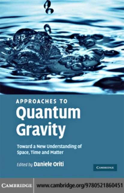
APPROACHES TO QUANTUM GRAVITYToward a New Understanding of Space, Time and MatterThe theory of quantum gravity promises a revolutionary new understandingof gravity and spacetime, valid from microscopic to cosmological distances.Research in this field involves an exciting blend of rigorous mathematics and boldspeculations, foundational questions and technical issues.Containing contributions from leading researchers in this field, this bookpresents the fundamental issues involved in the construction of a quantum theory ofgravity and building up a quantum picture of space and time. It introduces the mostcurrent approaches to this problem, and reviews their main achievements. Eachpart ends in questions and answers, in which the contributors explore the meritsand problems of the various approaches. This book provides a complete overviewof this field from the frontiers of theoretical physics research for graduate studentsand researchers.DANIELE ORITI is a Researcher at the Max Planck Institute for GravitationalPhysics, Potsdam, Germany, working on non-perturbative quantum gravity. Hehas previously worked at the Perimeter Institute for Theoretical Physics, Canada;the Institute for Theoretical Physics at Utrecht University, The Netherlands; andthe Department of Applied Mathematics and Theoretical Physics, University ofCambridge, UK. He is well known for his results on spin foam models, and isamong the leading researchers in the group field theory approach to quantumgravity.

APPROACHES TO QUANTUM GRAVITYToward a New Understanding of Space,Time and MatterEdited byDANIELE ORITIMax Planck Institute for Gravitational Physics,Potsdam, Germany

CAMBRIDGE UNIVERSITY PRESSCambridge, New York, Melbourne, Madrid, Cape Town, Singapore, São PauloCambridge University PressThe Edinburgh Building, Cambridge CB2 8RU, UKPublished in the United States of America by Cambridge University Press, New Yorkwww.cambridge.orgInformation on this title: www.cambridge.org/9780521860451© Cambridge University Press 2009This publication is in copyright. Subject to statutory exception and to theprovision of relevant collective licensing agreements, no reproduction of any partmay take place without the written permission of Cambridge University Press.First published in print format2009ISBN-13 978-0-511-51640-5ISBN-13 978-0-521-86045-1eBook (EBL)hardbackCambridge University Press has no responsibility for the persistence or accuracyof urls for external or third-party internet websites referred to in this publication,and does not guarantee that any content on such websites is, or will remain,accurate or appropriate.

A Sandra

ContentsList of contributorsPrefacepage xxvPart I Fundamental ideas and general formalisms 11 Unfinished revolution 3C. Rovelli2 The fundamental nature of space and time 13G. ’t Hooft3 Does locality fail at intermediate length scales? 26R. D. Sorkin4 Prolegomena to any future Quantum Gravity 44J. Stachel5 Spacetime symmetries in histories canonical gravity 68N. Savvidou6 Categorical geometry and the mathematicalfoundations of Quantum Gravity 84L. Crane7 Emergent relativity 99O. Dreyer8 Asymptotic safety 111R. Percacci9 New directions in background independent Quantum Gravity 129F. MarkopoulouQuestions and answers 150Part II String/M-theory 16710 Gauge/gravity duality 169G. Horowitz and J. Polchinskivii

viiiContents11 String theory, holography and Quantum Gravity 187T. Banks12 String field theory 210W. TaylorQuestions and answers 229Part III Loop quantum gravity and spin foam models 23313 Loop quantum gravity 235T. Thiemann14 Covariant loop quantum gravity? 253E. Livine15 The spin foam representation of loop quantum gravity 272A. Perez16 Three-dimensional spin foam Quantum Gravity 290L. Freidel17 The group field theory approach to Quantum Gravity 310D. OritiQuestions and answers 332Part IV Discrete Quantum Gravity 33918 Quantum Gravity: the art of building spacetime 341J. Ambjørn, J. Jurkiewicz and R. Loll19 Quantum Regge calculus 360R. Williams20 Consistent discretizations as a road to Quantum Gravity 378R. Gambini and J. Pullin21 The causal set approach to Quantum Gravity 393J. HensonQuestions and answers 414Part V Effective models and Quantum Gravity phenomenology 42522 Quantum Gravity phenomenology 427G. Amelino-Camelia23 Quantum Gravity and precision tests 450C. Burgess24 Algebraic approach to Quantum Gravity II: noncommutativespacetime 466S. Majid

Contentsix25 Doubly special relativity 493J. Kowalski-Glikman26 From quantum reference frames to deformed special relativity 509F. Girelli27 Lorentz invariance violation and its role in Quantum Gravityphenomenology 528J. Collins, A. Perez and D. Sudarsky28 Generic predictions of quantum theories of gravity 548L. SmolinQuestions and answers 571Index 580

ContributorsJ. AmbjørnThe Niels Bohr Institute, Copenhagen University, Blegdamsvej 17, DK-2100Copenhagen O, DenmarkandInstitute for Theoretical Physics, Utrecht University, Leuvenlaan 4,NL-3584 CE Utrecht, The NetherlandsG. Amelino-CameliaDipartimento di Fisica, Universitá di Roma “La Sapienza”, P.le A. Moro 2,00185 Rome, ItalyT. BanksDepartment of Physics, University of California, Santa Cruz, CA 95064, USAandNHETC, Rutgers University, Piscataway, NJ 08854, USAC. BurgessDepartment of Physics & Astronomy, McMaster University, 1280 Main St. W,Hamilton, Ontario, Canada, L8S 4M1andPerimeter Institute for Theoretical Physics, 31 Caroline St. N, Waterloo N2L2Y5, Ontario, CanadaJ. CollinsPhysics Department, Pennsylvania State University, University Park, PA 16802,USAL. CraneMathematics Department, Kansas State University, 138 Cardwell Hall Manhattan,KS 66506-2602, USAx

List of contributorsxiO. DreyerTheoretical Physics, Blackett Laboratory, Imperial College London, London, SW72AZ, UKL. FreidelPerimeter Institute for Theoretical Physics, 31 Caroline St. N, Waterloo N2L 2Y5,Ontario, CanadaR. GambiniInstituto de Física, Facultad de Ciencias, Iguá 4225, Montevideo, UruguayF. GirelliSISSA, via Beirut 4, Trieste, 34014, Italy, and INFN, sezione di Trieste, ItalyJ. HensonInstitute for Theoretical Physics, Utrecht University, Leuvenlaan 4, NL-3584 CEUtrecht, The NetherlandsG. HorowitzPhysics Department, University of California, Santa Barbara, CA 93106, USAJ. JurkiewiczInstitute of Physics, Jagellonian University, Reymonta 4, PL 30-059 Krakow,PolandJ. Kowalski-GlikmanInstitute for Theoretical Physics, University of Wroclaw 50-204 Wroclaw, pl. M.Borna 9, PolandE. LivineEcole Normale Supérieure de Lyon, 46 Allée d’Italie, 69364 Lyon Cedex 07, FranceR. LollInstitute for Theoretical Physics, Utrecht University, Leuvenlaan 4, NL-3584 CEUtrecht, The NetherlandsS. MajidSchool of Mathematical Sciences, Queen Mary, University of London327 Mile End Rd, London E1 4NS, UKandPerimeter Institute for Theoretical Physics, 31 Caroline St. N., Waterloo ON N2L2Y5, CanadaF. MarkopoulouPerimeter Institute for Theoretical Physics, 31 Caroline St. N., Waterloo ON N2L2Y5, Canada

xiiList of contributorsD. OritiMax Planck Institute for Gravitational Physics, Am Mühlenberg 1, D 14476 Golm,GermanyR. PercacciSISSA, via Beirut 4, Trieste, 34014, Italy, and INFN, sezione di Trieste, ItalyA. PerezCentre de Physique Théorique, Unité Mixte de Recherche (UMR 6207)du CNRS et des Universités Aix-Marseille I, Aix-Marseille II, et du Sud Toulon-Var,laboratoire afilié à la FRUMAM (FR 2291), Campus de Luminy, 13288 Marseille,FranceJ. PolchinskiDepartment of Physics, University of California, Santa Barbara CA 93106, USAJ. PullinDepartment of Physics and Astronomy, Louisiana State University, Baton Rouge,LA 70803 USAC. RovelliCentre de Physique Théorique, Unité Mixte de Recherche (UMR 6207)du CNRS et des Universités Aix-Marseille I, Aix-Marseille II, et du Sud Toulon-Var,laboratoire afilié à la FRUMAM (FR 2291), Campus de Luminy, 13288 Marseille,FranceN. SavvidouTheoretical Physics, Blackett Laboratory, Imperial College London, London SW72AZ, UKL. SmolinPerimeter Institute for Theoretical Physics, Waterloo N2J 2W9, Ontario, CanadaandDepartment of Physics, University of Waterloo, Waterloo N2L 3G1, Ontario,CanadaR. D. SorkinPerimeter Institute for Theoretical Physics, Waterloo N2J 2W9, Ontario, CanadaJ. StachelCAS Physics, Boston University, 745 Commonwealth Avenue, MA 02215, USAD. SudarskyInstituto de Ciencias Nucleares, Universidad Autónoma de México, A. P. 70-543,México D.F. 04510, México

List of contributorsxiiiW. TaylorMassachusetts Institute of Technology, Lab for Nuclear Science and Center forTheoretical Physics, 77 Massachusetts Ave., Cambridge, MA 02139-4307, USAT. ThiemannMax-Planck-Institut für Gravitationsphysik, Albert-Einstein-Institut,Am Mühlenberg 1, D-14476 Golm, GermanyandPerimeter Institute for Theoretical Physics, 31 Caroline St. North, Waterloo N2L2Y5, Ontario, CanadaG. ’t HooftInstitute for Theoretical Physics, Utrecht University, Leuvenlaan 4, NL-3584 CEUtrecht, The NetherlandsR. WilliamsDepartment of Applied Mathematics and Theoretical Physics, Centre forMathematical Sciences, University of Cambridge, Wilberforce Road, CambridgeCB3 0WA, UK

PrefaceQuantum Gravity is a dream, a theoretical need and a scientific goal. It is a theorywhich still does not exist in complete form, but that many people claim to have hadglimpses of, and it is an area of research which, at present, comprises the collectiveefforts of hundreds of theoretical and mathematical physicists.This yet-to-be-found theory promises to be a more comprehensive and completedescription of the gravitational interaction, a description that goes beyondEinstein’s General Relativity in being possibly valid at all scales of distances andenergy; at the same time it promises to provide a new and deeper understanding ofthe nature of space, time and matter.As such, research in Quantum Gravity is a curious and exciting blend of rigorousmathematics and bold speculations, concrete models and general schemata,foundational questions and technical issues, together with, since recently, tentativephenomenological scenarios.In the past three decades we have witnessed an amazing growth of the field ofQuantum Gravity, of the number of people actively working in it, and consequentlyof the results achieved. This is due to the fact that some approaches to the problemstarted succeeding in solving outstanding technical challenges, in suggestingways around conceptual issues, and in providing new physical insights and scenarios.A clear example is the explosion of research in string theory, one of the maincandidates to a quantum theory of gravity, and much more. Another is the developmentof Loop Quantum Gravity, an approach that attracted much attention recently,due to its successes in dealing with many long standing problems of the canonicalapproach to Quantum Gravity. New techniques have been then imported to the fieldfrom other areas of theoretical physics, e.g. Lattice Gauge Theory, and influencedin several ways the birth or growth of even more directions in Quantum Gravityresearch, including for example discrete approaches. At the same time, QuantumGravity has been a very fertile ground and a powerful motivation for developingxv

xviPrefacenew mathematics as well as alternative ways of thinking about spacetime and matter,which in turn have triggered the exploration of other promising avenues towarda Quantum Gravity theory.I think it is fair to say that we are still far from having constructed a satisfactorytheory of Quantum Gravity, and that any single approach currently beingconsidered is too incomplete or poorly understood, whatever its strengths and successesmay be, to claim to have achieved its goal, or to have proven to be the onlyreasonable way to proceed.On the other hand every single one of the various approaches being pursued hasachieved important results and insights regarding the Quantum Gravity problem.Moreover, technical or conceptual issues that are unsolved in one approach havebeen successfully tackled in another, and often the successes of one approach haveclearly come from looking at how similar difficulties had been solved in another.It is even possible that, in order to achieve our common goal, formulate a completetheory of Quantum Gravity and unravel the fundamental nature of space andtime, we will have to regard (at least some of) these approaches as different aspectsof the same theory, or to develop a more complete and more general approach thatcombines the virtues of several of them. However strong faith one may have in anyof these approaches, and however justified this may be in light of recent results,it should be expected, purely on historical grounds, that none of the approachescurrently pursued will be understood in the future in the same way as we do now,even if it proves to be the right way to proceed. Therefore, it is useful to lookfor new ideas and a different perspective on each of them, aided by the the insightsprovided by the others. In no area of research a “dogmatic approach” is less productive,I feel, than in Quantum Gravity, where the fundamental and complex natureof the problem, its many facets and long history, combined with a dramatically (buthopefully temporarily) limited guidance from Nature, suggest a very open-mindedattitude and a very critical and constant re-evaluation of one’s own strategies.I believe, therefore, that a broad and well-informed perspective on the variouspresent approaches to Quantum Gravity is a necessary tool for advancingsuccessfully in this area.This collective volume, benefiting from the contributions of some of the bestQuantum Gravity practitioners, all working at the frontiers of current research, ismeant to represent a good starting point and an up-to-date support reference, forboth students and active researchers in this fascinating field, for developing such abroader perspective. It presents an overview of some of the many ideas on the table,an introduction to several current approaches to the construction of a Quantum Theoryof Gravity, and brief reviews of their main achievements, as well as of the manyoutstanding issues. It does so also with the aim of offering a comparative perspectiveon the subject, and on the different roads that Quantum Gravity researchers

Prefacexviiare following in their searches. The focus is on non-perturbative aspects of QuantumGravity and on the fundamental structure of space and time. The variety ofapproaches presented is intended to ensure that a variety of ideas and mathematicaltechniques will be introduced to the reader.More specifically, the first part of the book (Part I) introduces the problem ofQuantum Gravity, and raises some of the fundamental questions that research inQuantum Gravity is trying to address. These concern for example the role of localityand of causality at the most fundamental level, the possibility of the notion ofspacetime itself being emergent, the possible need to question and revise our wayof understanding both General Relativity and Quantum Mechanics, before the twocan be combined and made compatible in a future theory of Quantum Gravity. Itprovides as well suggestions for new directions (using the newly available tools ofcategory theory, or quantum information theory, etc.) to explore both the constructionof a quantum theory of gravity, as well as our very thinking about space andtime and matter.The core of the book (Parts II–IV) is devoted to a presentation of severalapproaches that are currently being pursued, have recently achieved importantresults, and represent promising directions. Among these the most developed andmost practiced are string/M-theory, by far the one which involves at present thelargest amount of scholars, and loop quantum gravity (including its covariantversion, i.e. spin foam models). Alongside them, we have various (and rather differentin both spirit and techniques used) discrete approaches, represented hereby simplicial quantum gravity, in particular the recent direction of causal dynamicaltriangulations, quantum Regge calculus, and the “consistent discretizationscheme”, and by the causal set approach.All these approaches are presented at an advanced but not over-technical level,so that the reader is offered an introduction to the basic ideas characterizing anygiven approach as well as an overview of the results it has already achieved anda perspective on its possible development. This overview will make manifest thevariety of techniques and ideas currently being used in the field, ranging from continuum/analyticto discrete/combinatorial mathematical methods, from canonicalto covariant formalisms, from the most conservative to the most radical conceptualsettings.The final part of the book (Part V) is devoted instead to effective models ofQuantum Gravity. By this we mean models that are not intended to be of a fundamentalnature, but are likely to provide on the one hand key insights on whatsort of features the more fundamental formulation of the theory may possess, andon the other powerful tools for studying possible phenomenological consequencesof any Quantum Gravity theory, the future hopefully complete version as well

xviiiPrefaceas the current tentative formulations of it. The subject of Quantum Gravity phenomenologyis a new and extremely promising area of current research, and givesground to the hope that in the near future Quantum Gravity research may receiveexperimental inputs that will complement and direct mathematical insights andconstructions.The aim is to convey to the reader the recent insight that a Quantum Gravitytheory need not be forever detached by the experimental realm, and that manypossibilities for a Quantum Gravity phenomenology are instead currently open toinvestigation.At the end of each part, there is a “Questions & Answers” session. In each ofthem, the various contributors ask and put forward to each other questions, commentsand criticisms to each other, which are relevant to the specific topic coveredin that part. The purpose of these Q&A sessions is fourfold: (a) to clarify furthersubtle or particularly relevant features of the formalisms or perspectives presented;(b) to put to the forefront critical aspects of the various approaches, includingpotential difficulties or controversial issues; (c) to give the reader a glimpse of thereal-life, ongoing debates among scholars working in Quantum Gravity, of theirdifferent perspectives and of (some of) their points of disagreement; (d) in a sense,to give a better picture of how science and research (in particular, Quantum Gravityresearch) really work and of what they really are.Of course, just as the book as a whole cannot pretend to represent a completeaccount of what is currently going on in Quantum Gravity research, theseQ&A sessions cannot really be a comprehensive list of relevant open issues nor afaithful portrait of the (sometimes rather heated) debate among Quantum Gravityresearchers.What this volume makes manifest is the above-mentioned impressive developmentthat occurred in the field of Quantum Gravity as a whole, over the past, say,20–30 years. This is quickly recognized, for example, by comparing the range andcontent of the following contributed papers to the content of similar collective volumes,like Quantum Gravity 2: a second Oxford symposium, C. Isham, ed., OxfordUniversity Press (1982), Quantum structure of space and time, M. Duff, C. Isham,eds., Cambridge University Press (1982), Quantum Theory of Gravity, essays inhonor of the 60th Birthday of Bryce C DeWitt, S.D.Christensen,ed.,TaylorandFrancis (1984), or even the more recent Conceptual problems of Quantum Gravity,A. Ashtekar, J. Stachel, eds., Birkhauser (1991), all presenting overviews ofthe status of the subject at their time. Together with the persistence of the QuantumGravity problem itself, and of the great attention devoted, currently just asthen, to foundational issues alongside the more technical ones, it will be impossiblenot to notice the greater variety of current approaches, the extent to whichresearchers have explored beyond the traditional ones, and, most important, the

Prefacexixenormous amount of progress and achievements in each of them. Moreover, thevery existence of research in Quantum Gravity phenomenology was un-imaginableat the time.Quantum Gravity remains, as it was in that period, a rather esoteric subject,within the landscape of theoretical physics at large, but an active and fascinatingone, and one of fundamental significance. The present volume is indeed a collectivereport from the frontiers of theoretical physics research, reporting on the latest andmost exciting developments but also trying to convey to the reader the sense ofintellectual adventure that working at such frontiers implies.It is my pleasure to thank all those that have made the completion of this projectpossible. First of all, I gratefully thank all the researchers who have contributed tothis volume, reporting on their work and on the work of their colleagues in suchan excellent manner. This is a collective volume, and thus, if it has any value, it issolely due to all of them. Second, I am grateful to all the staff at the CambridgeUniversity Press, and in particular to Simon Capelin, for supporting this projectsince its conception, and for guiding me through its development. Last, I wouldlike to thank, for very useful comments, suggestions and advice, several colleaguesand friends: John Baez, Fay Dowker, Sean Hartnoll, Chris Isham, Prem Kumar,Pietro Massignan, and especially Ted Jacobson.Daniele Oriti

Part IFundamental ideas and general formalisms

1Unfinished revolutionC. ROVELLIOne hundred and forty-four years elapsed between the publication of Copernicus’sDe Revolutionibus, which opened the great scientific revolution of the seventeenthcentury, and the publication of Newton’s Principia, the final synthesis that broughtthat revolution to a spectacularly successful end. During those 144 years, the basicgrammar for understanding the physical world changed and the old picture ofreality was reshaped in depth.At the beginning of the twentieth century, General Relativity (GR) and QuantumMechanics (QM) once again began reshaping our basic understanding of space andtime and, respectively, matter, energy and causality – arguably to a no lesser extent.But we have not been able to combine these new insights into a novel coherentsynthesis, yet. The twentieth-century scientific revolution opened by GR and QMis therefore still wide open. We are in the middle of an unfinished scientific revolution.Quantum Gravity is the tentative name we give to the “synthesis to befound”.In fact, our present understanding of the physical world at the fundamental levelis in a state of great confusion. The present knowledge of the elementary dynamicallaws of physics is given by the application of QM to fields, namely QuantumField Theory (QFT), by the particle-physics Standard Model (SM), and by GR.This set of fundamental theories has obtained an empirical success nearly uniquein the history of science: so far there isn’t any clear evidence of observed phenomenathat clearly escape or contradict this set of theories – or a minor modification ofthe same, such as a neutrino mass or a cosmological constant. 1 But, the theories inthis set are based on badly self-contradictory assumptions. In GR the gravitationalfield is assumed to be a classical deterministic dynamical field, identified with the(pseudo) Riemannian metric of spacetime: but with QM we have understood thatall dynamical fields have quantum properties. The other way around, conventional1 Dark matter (not dark energy) might perhaps be contrary evidence.Approaches to Quantum Gravity: Toward a New Understanding of Space, Time and Matter, ed. Daniele Oriti.Published by Cambridge University Press. c○ Cambridge University Press 2009.

4 C. RovelliQFT relies heavily on global Poincaré invariance and on the existence of anon-dynamical background spacetime metric: but with GR we have understoodthat there is no such non-dynamical background spacetime metric in nature.In spite of their empirical success, GR and QM offer a schizophrenic and confusedunderstanding of the physical world. The conceptual foundations of classicalGR are contradicted by QM and the conceptual foundation of conventional QFTare contradicted by GR. Fundamental physics is today in a peculiar phase of deepconceptual confusion.Some deny that such a major internal contradiction in our picture of nature exists.On the one hand, some refuse to take QM seriously. They insist that QM makes nosense, after all, and therefore the fundamental world must be essentially classical.This doesn’t put us in a better shape, as far as our understanding of the world isconcerned.Others, on the other hand, and in particular some hard-core particle physicists, donot accept the lesson of GR. They read GR as a field theory that can be consistentlyformulated in full on a fixed metric background, and treated within conventionalQFT methods. They motivate this refusal by insisting than GR’s insight should notbe taken too seriously, because GR is just a low-energy limit of a more fundamentaltheory. In doing so, they confuse the details of the Einstein’s equations (whichmight well be modified at high energy), with the new understanding of space andtime brought by GR. This is coded in the background independence of the fundamentaltheory and expresses Einstein’s discovery that spacetime is not a fixed background,as was assumed in special relativistic physics, but rather a dynamical field.Nowadays this fact is finally being recognized even by those who have longrefused to admit that GR forces a revolution in the way to think about space andtime, such as some of the leading voices in string theory. In a recent interview[1], for instance, Nobel laureate David Gross says: “ [...] this revolution will likelychange the way we think about space and time, maybe even eliminate them completelyas a basis for our description of reality”. This is of course something thathas been known since the 1930s [2] by anybody who has taken seriously the problemof the implications of GR and QM. The problem of the conceptual novelty ofGR, which the string approach has tried to throw out of the door, comes back bythe window.These and others remind me of Tycho Brahe, who tried hard to conciliate Copernicus’sadvances with the “irrefutable evidence” that the Earth is immovable at thecenter of the universe. To let the background spacetime go is perhaps as difficultas letting go the unmovable background Earth. The world may not be the way itappears in the tiny garden of our daily experience.Today, many scientists do not hesitate to take seriously speculations such asextra dimensions, new symmetries or multiple universes, for which there isn’t a

Unfinished revolution 5wit of empirical evidence; but refuse to take seriously the conceptual implicationsof the physics of the twentieth century with the enormous body of empirical evidencesupporting them. Extra dimensions, new symmetries, multiple universes andthe like, still make perfectly sense in a pre-GR, pre-QM, Newtonian world,while to take GR and QM seriously together requires a genuine reshaping of ourworld view.After a century of empirical successes that have equals only in Newton’s andMaxwell’s theories, it is time to take seriously GR and QM, with their full conceptualimplications; to find a way of thinking the world in which what we havelearned with QM and what we have learned with GR make sense together – finallybringing the twentieth-century scientific revolution to its end. This is the problemof Quantum Gravity.1.1 Quantum spacetimeRoughly speaking, we learn from GR that spacetime is a dynamical field and welearn from QM that all dynamical field are quantized. A quantum field has a granularstructure, and a probabilistic dynamics, that allows quantum superposition ofdifferent states. Therefore at small scales we might expect a “quantum spacetime”formed by “quanta of space” evolving probabilistically, and allowing “quantumsuperposition of spaces”. The problem of Quantum Gravity is to give a precisemathematical and physical meaning to this vague notion of “quantum spacetime”.Some general indications about the nature of quantum spacetime, and onthe problems this notion raises, can be obtained from elementary considerations.The size of quantum mechanical effects is determined by Planck’s constant .Thestrength of the gravitational force is determined by Newton’s constant G, and therelativistic domain is determined by the speed of light c. By combining these threefundamental constants we obtain the Planck length l P = √ G/c 3 ∼ 10 −33 cm.Quantum-gravitational effects are likely to be negligible at distances much largerthan l P , because at these scales we can neglect quantities of the order of G, or 1/c.Therefore we expect the classical GR description of spacetime as a pseudo-Riemannian space to hold at scales larger than l P , but to break down approachingthis scale, where the full structure of quantum spacetime becomes relevant. QuantumGravity is therefore the study of the structure of spacetime at the Planckscale.1.1.1 SpaceMany simple arguments indicate that l P may play the role of a minimal length, inthe same sense in which c is the maximal velocity and the minimal exchangedaction.

6 C. RovelliFor instance, the Heisenberg principle requires that the position of an object ofmass m can be determined only with uncertainty x satisfying mvx > , where vis the uncertainty in the velocity; special relativity requires v Gm/c 2 , after which the region itself collapses into a black hole,subtracting itself from our observation. Combining these inequalities we obtainx > l P . That is, gravity, relativity and quantum theory, taken together, appear toprevent position from being determined more precisely than the Planck scale.A number of considerations of this kind have suggested that space might not beinfinitely divisible. It may have a quantum granularity at the Planck scale, analogousto the granularity of the energy in a quantum oscillator. This granularity ofspace is fully realized in certain Quantum Gravity theories, such as loop QuantumGravity, and there are hints of it also in string theory. Since this is a quantumgranularity, it escapes the traditional objections to the atomic nature of space.1.1.2 TimeTime is affected even more radically by the quantization of gravity. In conventionalQM, time is treated as an external parameter and transition probabilities changein time. In GR there is no external time parameter. Coordinate time is a gaugevariable which is not observable, and the physical variable measured by a clock isa nontrivial function of the gravitational field. Fundamental equations of QuantumGravity might therefore not be written as evolution equations in an observable timevariable. And in fact, in the quantum-gravity equation par excellence, the Wheeler–deWitt equation, there is no time variable t at all.Much has been written on the fact that the equations of nonperturbative QuantumGravity do not contain the time variable t. This presentation of the “problem oftime in Quantum Gravity”, however, is a bit misleading, since it mixes a problemof classical GR with a specific Quantum Gravity issue. Indeed, classical GR aswell can be entirely formulated in the Hamilton–Jacobi formalism, where no timevariable appears either.In classical GR, indeed, the notion of time differs strongly from the one used inthe special-relativistic context. Before special relativity, one assumed that there isa universal physical variable t, measured by clocks, such that all physical phenomenacan be described in terms of evolution equations in the independent variable t.In special relativity, this notion of time is weakened. Clocks do not measure a universaltime variable, but only the proper time elapsed along inertial trajectories. Ifwe fix a Lorentz frame, nevertheless, we can still describe all physical phenomenain terms of evolution equations in the independent variable x 0 , even though thisdescription hides the covariance of the system.

Unfinished revolution 7In general relativity, when we describe the dynamics of the gravitational field(not to be confused with the dynamics of matter in a given gravitational field),there is no external time variable that can play the role of observable independentevolution variable. The field equations are written in terms of an evolution parameter,which is the time coordinate x 0 ; but this coordinate does not correspond toanything directly observable. The proper time τ along spacetime trajectories cannotbe used as an independent variable either, as τ is a complicated non-localfunction of the gravitational field itself. Therefore, properly speaking, GR doesnot admit a description as a system evolving in terms of an observable time variable.This does not mean that GR lacks predictivity. Simply put, what GR predictsare relations between (partial) observables, which in general cannot be representedas the evolution of dependent variables on a preferred independent timevariable.This weakening of the notion of time in classical GR is rarely emphasized: afterall, in classical GR we may disregard the full dynamical structure of the theory andconsider only individual solutions of its equations of motion. A single solution ofthe GR equations of motion determines “a spacetime”, where a notion of propertime is associated to each timelike worldline.But in the quantum context a single solution of the dynamical equation is like asingle “trajectory” of a quantum particle: in quantum theory there are no physicalindividual trajectories: there are only transition probabilities between observableeigenvalues. Therefore in Quantum Gravity it is likely to be impossible to describethe world in terms of a spacetime, in the same sense in which the motion of aquantum electron cannot be described in terms of a single trajectory.To make sense of the world at the Planck scale, and to find a consistent conceptualframework for GR and QM, we might have to give up the notion of timealtogether, and learn ways to describe the world in atemporal terms. Time might bea useful concept only within an approximate description of the physical reality.1.1.3 Conceptual issuesThe key difficulty of Quantum Gravity may therefore be to find a way to understandthe physical world in the absence of the familiar stage of space and time. Whatmight be needed is to free ourselves from the prejudices associated with the habitof thinking of the world as “inhabiting space” and “evolving in time”.Technically, this means that the quantum states of the gravitational field cannotbe interpreted like the n-particle states of conventional QFT as living on a givenspacetime. Rather, these quantum states must themselves determine and define aspacetime – in the manner in which the classical solutions of GR do.

8 C. RovelliConceptually, the key question is whether or not it is logically possible to understandthe world in the absence of fundamental notions of time and time evolution,and whether or not this is consistent with our experience of the world.The difficulties of Quantum Gravity are indeed largely conceptual. Progress inQuantum Gravity cannot be just technical. The search for a quantum theory of gravityraises once more old questions such as: What is space? What is time? What isthe meaning of “moving”? Is motion to be defined with respect to objects or withrespect to space? And also: What is causality? What is the role of the observerin physics? Questions of this kind have played a central role in periods of majoradvances in physics. For instance, they played a central role for Einstein, Heisenberg,and Bohr; but also for Descartes, Galileo, Newton and their contemporaries,as well as for Faraday and Maxwell.Today some physicists view this manner of posing problems as “too philosophical”.Many physicists of the second half of the twentieth century, indeed, haveviewed questions of this nature as irrelevant. This view was appropriate for theproblems they were facing. When the basics are clear and the issue is problemsolvingwithin a given conceptual scheme, there is no reason to worry aboutfoundations: a pragmatic approach is the most effective one. Today the kind ofdifficulties that fundamental physics faces has changed. To understand quantumspacetime, physics has to return, once more, to those foundational questions.1.2 Where are we?Research in Quantum Gravity developed slowly for several decades during thetwentieth century, because GR had little impact on the rest of physics and the interestof many theoreticians was concentrated on the development of quantum theoryand particle physics. In the past 20 years, the explosion of empirical confirmationsand concrete astrophysical, cosmological and even technological applications ofGR on the one hand, and the satisfactory solution of most of the particle physicspuzzles in the context of the SM on the other, have led to a strong concentration ofinterest in Quantum Gravity, and the progress has become rapid. Quantum Gravityis viewed today by many as the big open challenge in fundamental physics.Still, after 70 years of research in Quantum Gravity, there is no consensus, andno established theory. I think it is fair to say that there isn’t even a single completeand consistent candidate for a quantum theory of gravity.In the course of 70 years, numerous ideas have been explored, fashions havecome and gone, the discovery of the Holy Grail of Quantum Gravity has beenseveral times announced, only to be later greeted with much scorn. Of the tentativetheories studied today (strings, loops and spinfoams, non-commutative geometry,dynamical triangulations or others), each is to a large extent incomplete and nonehas yet received a whit of direct or indirect empirical support.

Unfinished revolution 9However, research in Quantum Gravity has not been meandering meaninglessly.On the contrary, a consistent logic has guided the development of the research,from the early formulation of the problem and of the major research programs in the1950s to the present. The implementation of these programs has been laborious, buthas been achieved. Difficulties have appeared, and solutions have been proposed,which, after much difficulty, have lead to the realization, at least partial, of theinitial hopes.It was suggested in the early 1970s that GR could perhaps be seen as the lowenergy limit of a Poincaré invariant QFT without uncontrollable divergences [3];and today, 30 years later, a theory likely to have these properties – perturbativestring theory – is known. It was also suggested in the early 1970s that nonrenormalizabilitymight not be fatal for quantum GR [4; 5] and that the Planckscale could cut divergences off nonperturbatively by inducing a quantum discretestructure of space; and today we know that this is in fact the case – ultravioletfiniteness is realized precisely in this manner in canonical loop Quantum Gravityand in some spinfoam models. In 1957 Charles Misner indicated that in thecanonical framework one should be able to compute quantum eigenvalues of geometricalquantities [6]; and in 1995, 37 years later, eigenvalues of area and volumewere computed – within loop quantum gravity [7; 8]. Much remains to be understoodand some of the current developments might lead nowhere. But looking atthe entire development of the subject, it is difficult to deny that there has beensubstantial progress.In fact, at least two major research programs can today claim to have, if not acomplete candidate theory of Quantum Gravity, at least a large piece of it: stringtheory (in its perturbative and still incomplete nonperturbative versions) and loopquantum gravity (in its canonical as well as covariant – spinfoam – versions) areboth incomplete theories, full of defects – in general, strongly emphasized withinthe opposite camp – and without any empirical support, but they are both remarkablyrich and coherent theoretical frameworks, that might not be far from thesolution of the puzzle.Within these frameworks, classical and long intractable, physical, astrophysicaland cosmological Quantum Gravity problems can finally be concretely treated.Among these: black hole’s entropy and fate, the physics of the big-bang singularityand the way it has affected the currently observable universe, and many others.Tentative predictions are being developed, and the attention to the concrete possibilityof testing these predictions with observations that could probe the Planckscale is very alive. All this was unthinkable only a few years ago.The two approaches differ profoundly in their hypotheses, achievements, specificresults, and in the conceptual frame they propose. The issues they raise concernthe foundations of the physical picture of the world, and the debate betweenthe two approaches involves conceptual, methodological and philosophical issues.

10 C. RovelliIn addition, a number of other ideas, possibly alternative, possibly complementaryto the two best developed theories and to one another, are being explored.These include noncommutative geometry, dynamical triangulations, effective theories,causal sets and many others.The possibility that none of the currently explored hypotheses will eventuallyturn out to be viable, or, simply, none will turn out to be the way chosen by Nature,is very concrete, and should be clearly kept in mind. But the rapid and multi-frontprogress of the past few years raises hopes. Major well-posed open questions in theoreticalphysics (Copernicus or Ptolemy? Galileo’s parabolas or Kepler’s ellipses?How to describe electricity and magnetism? Does Maxwell theory pick a preferredreference frame? How to do the Quantum Mechanics of interacting fields...?) haverarely been solved in a few years. But they have rarely resisted more than a fewdecades. Quantum Gravity – the problem of describing the quantum properties ofspacetime – is one of these major problems, and it is reasonably well defined: isthere a coherent theoretical framework consistent with quantum theory and withGeneral Relativity? It is a problem which is on the table since the 1930s, but itis only in the past couple of decades that the efforts of the theoretical physicscommunity have concentrated on it.Maybe the solution is not far away. In any case, we are not at the end of the roadof physics, we are half-way through the woods along a major scientific revolution.Bibliographical noteFor details on the history of Quantum Gravity see the historical appendix in [9];and, for early history see [10; 11] and[12; 13]. For orientation on current researchon Quantum Gravity, see the review papers [14; 15; 16; 17]. As a general introductionto Quantum Gravity ideas, see the old classic reviews, which are rich inideas and present different points of view, such as John Wheeler 1967 [18], StevenWeinberg 1979 [5], Stephen Hawking 1979 and 1980 [19; 20], Karel Kuchar 1980[21], and Chris Isham’s magisterial syntheses [22; 23; 24]. On string theory, classictextbooks are Green, Schwarz and Witten, and Polchinksi [25; 26]. On loop quantumgravity, including the spinfoam formalism, see [9; 27; 28], or the older papers[29; 30]. On spinfoams see also [31]. On noncommutative geometry see [32] andon dynamical triangulations see [33]. For a discussion of the difficulties of stringtheory and a comparison of the results of strings and loops, see [34], written in theform of a dialogue, and [35]. On the more philosophical challenges raised by QuantumGravity, see [36]. Smolin’s popular book [37] provides a readable introductionto Quantum Gravity. The expression “half way through the woods” to characterizethe present state of fundamental theoretical physics is taken from [38; 39]. My ownview on Quantum Gravity is developed in detail in [9].

Unfinished revolution 11References[1] D. Gross, 2006, in Viewpoints on string theory, NOVA science programming on airand online, http://www.pbs.org/wgbh/nova/elegant/view-gross.html.[2] M.P. Bronstein, “Quantentheories schwacher Gravitationsfelder”, PhysikalischeZeitschrift der Sowietunion 9 (1936), 140.[3] B. Zumino, “Effective Lagrangians and broken symmetries”, in Brandeis UniversityLectures On Elementary Particles And Quantum Field Theory, Vol 2 (Cambridge,Mass, 1970), pp. 437–500.[4] G. Parisi, “The theory of non-renormalizable interactions. 1 The large N expansion”,Nucl Phys B100 (1975), 368.[5] S. Weinberg, “Ultraviolet divergences in quantum theories of gravitation”, inGeneral Relativity: An Einstein Centenary Survey, S. W. Hawking and W. Israel,eds. (Cambridge University Press, Cambridge, 1979).[6] C. Misner, “Feynman quantization of general relativity”, Rev. Mod. Phys. 29 (1957),497.[7] C. Rovelli, L. Smolin, “Discreteness of area and volume in quantum gravity”,Nucl. Phys. B442 (1995) 593; Erratum Nucl. Phys. B456 (1995), 734.[8] A. Ashtekar, J. Lewandowski, “Quantum theory of geometry I: area operators”Class and Quantum Grav 14 (1997) A55; “II : volume operators”, Adv. Theo. Math.Phys. 1 (1997), pp. 388–429.[9] C. Rovelli, Quantum Gravity (Cambridge University Press, Cambridge, 2004).[10] J. Stachel, “Early history of quantum gravity (1916–1940)”, Presented at the HGR5,Notre Dame, July 1999.[11] J. Stachel, “Early history of quantum gravity” in ‘Black Holes, Gravitationalradiation and the Universe, B. R. Iyer and B. Bhawal, eds. (Kluwer AcademicPublisher, Netherlands, 1999).[12] G. E. Gorelik, “First steps of quantum gravity and the Planck values” in Studies inthe history of general relativity. [Einstein Studies, vol. 3], J. Eisenstaedt and A. J.Kox, eds., pp. 364–379 (Birkhaeuser, Boston, 1992).[13] G. E. Gorelik, V. Y. Frenkel, Matvei Petrovic Bronstein and the Soviet TheoreticalPhysics in the Thirties (Birkhauser Verlag, Boston 1994).[14] G. Horowitz, “Quantum gravity at the turn of the millenium”, plenary talk at theMarcel Grossmann conference, Rome 2000, gr-qc/0011089.[15] S. Carlip, “Quantum gravity: a progress report”, Reports Prog. Physics 64 (2001)885, gr-qc/0108040.[16] C. J. Isham, “Conceptual and geometrical problems in quantum gravity”, in RecentAspects of Quantum fields, H. Mitter and H. Gausterer, eds. (Springer Verlag, Berlin,1991), p. 123.[17] C. Rovelli, “Strings, loops and the others: a critical survey on the present approachesto quantum gravity”, in Gravitation and Relativity: At the Turn of the Millenium,N. Dadhich and J. Narlikar, eds., pp. 281–331 (Inter-University Centre forAstronomy and Astrophysics, Pune, 1998), gr-qc/9803024.[18] J. A. Wheeler, “Superspace and the nature of quantum geometrodynamics”, inBatelle Rencontres, 1967, C. DeWitt and J. W. Wheeler, eds., Lectures inMathematics and Physics, 242 (Benjamin, New York, 1968).[19] S. W. Hawking, “The path-integral approach to quantum gravity”, in GeneralRelativity: An Einstein Centenary Survey, S. W. Hawking and W. Israel, eds.(Cambridge University Press, Cambridge, 1979).

12 C. Rovelli[20] S. W. Hawking, “Quantum cosmology”, in Relativity, Groups and Topology, LesHouches Session XL, B. DeWitt and R. Stora, eds. (North Holland, Amsterdam,1984).[21] K. Kuchar, “Canonical methods of quantization”, in Oxford 1980, Proceedings,Quantum Gravity 2 (Oxford University Press, Oxford, 1984).[22] C. J. Isham, Topological and global aspects of quantum theory, in Relativity Groupsand Topology. Les Houches 1983, B. S. DeWitt and R. Stora, eds. (North Holland,Amsterdam, 1984), pp. 1059–1290.[23] C. J. Isham, “Quantum gravity: an overview”, in Oxford 1980, Proceedings,Quantum Gravity 2 (Oxford University Press, Oxford, 1984).[24] C. J. Isham, 1997, “Structural problems facing quantum gravity theory”, inProceedings of the 14th International Conference on General Relativity andGravitation, M. Francaviglia, G. Longhi, L. Lusanna and E. Sorace, eds., (WorldScientific, Singapore, 1997), pp 167–209.[25] M. B. Green, J. Schwarz, E. Witten, Superstring Theory (Cambridge UniversityPress, Cambridge, 1987).[26] J. Polchinski, String Theory (Cambridge University Press, Cambridge, 1998).[27] T. Thiemann, Introduction to Modern Canonical Quantum General Relativity,(Cambridge University Press, Cambridge, in the press).[28] A. Ashtekar, J. Lewandowski, “Background independent quantum gravity: A statusreport”, Class. Quant. Grav. 21 (2004), R53–R152.[29] C. Rovelli, L. Smolin, “Loop space representation for quantum general relativity,Nucl. Phys. B331 (1990), 80.[30] C. Rovelli, L. Smolin, “Knot theory and quantum gravity”, Phys. Rev. Lett. 61(1988), 1155.[31] A. Perez, “Spin foam models for quantum gravity”, Class. Quantum Grav. 20(2002), gr-qc/0301113.[32] A. Connes, Non Commutative Geometry (Academic Press, New York, 1994).[33] R. Loll, “Discrete approaches to quantum gravity in four dimensions”, Liv. Rev. Rel.1 (1998), 13, http://www.livingreviews.org/lrr-1998-13.[34] C. Rovelli, “A dialog on quantum gravity”, International Journal of Modern Physics12 (2003), 1, hep-th/0310077.[35] L. Smolin, “How far are we from the quantum theory of gravity?” (2003),hep-th/0303185.[36] C. Callender, H. Huggett, eds, Physics Meets Philosophy at the Planck Scale(Cambridge University Press, 2001).[37] L. Smolin, Three Roads to Quantum Gravity (Oxford University Press, 2000).[38] C. Rovelli, “Halfway through the woods”, in The Cosmos of Science, J. Earman andJ. D. Norton, eds. (University of Pittsburgh Press and Universitäts. Verlag-Konstanz,1997).[39] C. Rovelli, “The century of the incomplete revolution: searching for generalrelativistic quantum field theory”, J. Math. Phys., Special Issue 2000 41(2000), 3776.

2The fundamental nature of space and timeG. ’T HOOFT2.1 Quantum Gravity as a non-renormalizable gauge theoryQuantum Gravity is usually thought of as a theory, under construction, where thepostulates of quantum mechanics are to be reconciled with those of general relativity,without allowing for any compromise in either of the two. As will be arguedin this contribution, this ‘conservative’ approach may lead to unwelcome compromisesconcerning locality and even causality, while more delicate and logicallymore appealing schemes can be imagined.The conservative procedure, however, must first be examined closely. The firstattempt (both historically and logically the first one) is to formulate the theory of‘Quantum Gravity’ perturbatively [1; 2; 3; 4; 5], as has been familiar practice in thequantum field theories for the fundamental particles, namely the Standard Model.In perturbative Quantum Gravity, one takes the Einstein–Hilbert action,∫S = ∂ 4 x √ ( R(x))−g + L matter (x) ɛ = 16πG (2.1)ɛconsiders the metric to be close to some background value: g μν = gμν Bg + √ ɛ h μν ,and expands everything in powers of ɛ, or equivalently, Newton’s constant G.Invariance under local coordinate transformations then manifests itself as a localgauge symmetry: h μν 〉h μν + D μ u ν + D ν u μ , where D μ is the usual covariant derivative,and u μ (x) generates an infinitesimal coordinate transformation. Here one canuse the elaborate machinery that has been developed for the Yang–Mills theories ofthe fundamental particles. After imposing an appropriate gauge choice, all desiredamplitudes can be characterized in terms of Feynman diagrams. Usually, these containcontributions of ‘ghosts’, which are gauge dependent degrees of freedom thatpropagate according to well-established rules. At first sight, therefore, QuantumGravity does not look altogether different from a Yang–Mills theory. It appearsthat at least the difficulties of reconciling quantum mechanics with general coordinateinvariance have been dealt with. We understand exactly how the problemApproaches to Quantum Gravity: Toward a New Understanding of Space, Time and Matter, ed. Daniele Oriti.Published by Cambridge University Press. c○ Cambridge University Press 2009.

14 G. ’t Hooftof time, of Cauchy surfaces, and of picking physical degrees of freedom, are tobe handled in such a formalism. Indeed, unitarity is guaranteed in this formalism,and, in contrast to ‘more advanced’ schemes for quantizing gravity, the perturbativeapproach can deal adequately with problems such as: what is the completeHilbert space of physical states?, how can the fluctuations of the light cone besquared with causality?, etc., simply because at all finite orders in perturbationexpansion, such serious problems do not show up. Indeed, this is somewhat surprising,because the theory produces useful amplitudes at all orders of the perturbationparameter ɛ.Yet there is a huge difference with the Standard Model. This ‘quantum gauge theoryof gravity’ is not renormalizable. We must distinguish the technical difficultyfrom the physical one. Technically, the ‘disaster’ of having a non-renormalizabletheory is not so worrisome. In computing the O(ɛ n ) corrections to some amplitude,one has to establish O(ɛ n ) correction terms to the Lagrangian, which are typicallyof the form √ −gR n+1 , where n + 1 factors linear in the Riemann curvature R α βμνmay have been contracted in various possible ways. These terms are necessary tocancel out infinite counter terms of this form, where finite parts are left over. Athigh orders n, there exist many different expressions of the form R n+1 , which willall be needed. This is often presented as a problem, but, in principle, it is not.It simply means that our theory has an infinite sequence of free parameters, notunlike many other theories in science, and it nevertheless gives accurate and usefulpredictions up to arbitrarily high powers of GE 2 , where E is the energy scale considered.We emphasize that this is actually much better than many of the alternativeapproaches to Quantum Gravity such as Loop Quantum Gravity, and even stringtheory presents us with formidable problems when 3-loop amplitudes are asked for.Also, claims [6] that Quantum Gravity effects might cause ‘decoherence’ at somefinite order of GE 2 are invalid according to this theory.Physically, however, the perturbative approach fails. The difficulty is not the factthat the finite parts of the counter terms can be freely chosen. The difficulty is acombination of two features: (i) perturbation expansion does not converge, and (ii)the expansion parameter becomes large if centre-of-mass energies reach beyond thePlanck value. The latter situation is very reminiscent of the old weak interactiontheory where a quartic interaction was assumed among the fermionic fields. ThisFermi theory was also ‘non-renormalizable’.In the Fermi theory, this problem was solved: the theory was replaced by aYang–Mills theory with Brout–Englert–Higgs mechanism. This was not just ‘away to deal with the infinities’, it was actually an answer to an absolutely crucialquestion [7]: what happens at small distance scales?. At small distance scales,we do not have quartic interactions among fermionic fields, we have a local gaugetheory instead. This is actually also the superior way to phrase the problem of

The fundamental nature of space and time 15Quantum Gravity: what happens at, or beyond, the Planck scale? Superstring theory[8; 9] is amazingly evasive if it comes to considering this question. It is herethat Loop Quantum Gravity [10; 11; 12; 13; 14; 15] appears to be the most directapproach. It is an attempt to characterize the local degrees of freedom, but is itgood enough?2.2 A prototype: gravitating point particles in 2 + 1 dimensionsAn instructive exercise is to consider gravity in less than four space-time dimensions.Indeed, removing two dimensions allows one to formulate renormalizablemodels with local diffeomorphism invariance. Models of this sort, having onespace- and one time dimension, are at the core of (super)string theory, where theydescribe the string world sheet. In such a model, however, there is no large distancelimit with conventional ‘gravity’, so it does not give us hints on how to curenon-renormalizable long-distance features by modifying its small distance characteristics.There is also another reason why these two-dimensional models areuncharacteristic for conventional gravity: formally, pure gravity in d = 2 dimensionshas 1 d(d − 3) =−1 physical degrees of freedom, which means that an2additional scalar field is needed to turn the theory into a topological theory. Conformalsymmetry removes one further degree of freedom, so that, if string theorystarts with D target space variables, or ‘fields’, X μ (σ, Tr), where μ = 1, ··· , D,only D − 2 physical fields remain.For the present discussion it is therefore more useful to remove just one dimension.Start with gravitationally interacting point particles in two space dimensionsand one time. The classical theory is exactly solvable, and this makes it very interesting.Gravity itself, having zero physical degrees of freedom, is just topological;there are no gravitons, so the physical degrees of freedom are just the gravitatingpoint particles. In the large distance limit, where Quantum Mechanical effects maybe ignored, the particles are just point defects surrounded by locally flat space-time.The dynamics of these point defects has been studied [16; 17; 18], and the evolutionlaws during finite time intervals are completely understood. During very longtime intervals, however, chaotic behavior sets in, and also, establishing a completelist of all distinguishable physical states turns out to be a problem. One might havethought that quantizing a classically solvable model is straightforward, but it isfar from that, exactly because of the completeness problem. 2 + 1 gravity withoutpoint particles could be quantized [19; 20], but that is a topological theory, with nolocal degrees of freedom; all that is being quantized are the boundary conditions,whatever that means.One would like to represent the (non-rotating) point particles by some scalarfield theory, but the problems one then encounters appear to be formidable. Quite

16 G. ’t Hooftgenerally, in 2 + 1 dimensions, the curvature of 2-space is described by defectangles when following closed curves (holonomies). The total defect angle accumulatedby a given closed curve always equals the total matter-energy enclosed bythe curve. In the classical model, all of this is crystal clear. But what happens whenone attempts to ‘quantize’ it? The matter Hamiltonian density does not commutewith any of the particle degrees of freedom, since the latter evolve as a functionof time. Thus, anything that moves, is moving in a space-time whose curvature isnon-commuting. This is an impediment against a proper formulation of the Hilbertspace in question in the conventional manner. Only eigenstates of the Hamiltonianand the Hamiltonian density can live in a 2-space with precisely defined 2-metric.Consequently, if we wish to describe physical states in a 2-space with preciselydefined metric, these states must be smeared over a period of time that is largecompared to the Planck time. We repeat: in a perturbative setting this situation canbe handled because the deviations from flat space-time are small, but in a nonperturbativecase, we have to worry about the limits of the curvature. The deficitangles cannot exceed the value 2π, and this implies that the Hamilton density mustbe bounded.There is, however, an unconventional quantization procedure that seems to bequite appropriate here. We just noted that the Hamiltonian of this theory is unmistakablyan angle, and this implies that time, its conjugate variable, must becomediscrete as soon as we quantize. Having finite time jumps clearly indicates in whatdirection we should search for a satisfactory quantum model: Schrödinger’s equationwill be a finite difference equation in the time direction. Take that as a modifiedpicture for the small-distance structure of the theory!How much more complicated will the small-distance structure be in our 3 + 1dimensional world? Here, the Hamiltonian is not limited to be an angle, so, timewill surely be continuous. However, if we restrict ourselves to a region where oneor more spatial dimensions are taken to be confined, or compactified, taking valuessmaller than some scale L in Planck units, then it is easy to see that we are backin the 2 + 1 dimensional case, the Hamiltonian is again an angle, and time will bequantized. However, the 2 + 1 dimensional Newton’s constant will scale like 1/L,and the time quantum will therefore be of order 1/L in Planck units. This suggeststhe following. In finite slabs of 3-space, time is quantized, the states are ‘updated’in discretized time steps. If we stitch two equal sized slabs together, producing aslab twice as thick, then updating happens twice as fast, which we interpret as ifupdating happens alternatingly in one slab and in the other. The total time quantumhas decreased by a factor two, but within each slab, time is still quantized in theoriginal units. The picture we get this way is amazingly reminiscent of a computermodel, where the computer splits 3-space into slabs of one Planck length thick, andduring one Planck time interval every slab is being updated; a stack of N slabs thusrequires N updates per Planck unit of time.

The fundamental nature of space and time 172.3 Black holes, causality and localityThe 2 + 1 dimensional theory does not allow for the presence of black holes(assuming a vanishing cosmological constant, as we will do throughout). The blackhole problem, there, is simply replaced by the restriction that the energy must stayless than the Planck value. In our slab-stack theory (for want of a better name), wesee that the energy in every slab is restricted to be less than the Planck value, so anysystem where one of the linear dimensions is less than L, should have energy lessthan L in Planck units, and this amounts to having a limit for the total energy thatis such that a black hole corresponds to the maximally allowed energy in a givenregion.Clearly, black holes will be an essential element in any Quantum Gravity theory.We must understand how to deal with the requirement that the situation obtainedafter some gravitational collapse can be either described as some superdense blobof mass and energy, or as a geometric region of space-time itself where ingoingobservers should be allowed to apply conventional laws of physics to describe whatthey see.One can go a long way to deduce the consequences of this requirement. Particlesgoing into a black hole will interact with all particles going out. Of all these interactions,the gravitational one happens to play a most crucial role. Only by takingthis interaction into account [21], can one understand how black holes can playthe role of resonances in a unitary scattering process where ingoing particles formblack holes and outgoing particles are the ones generated by the Hawking process.Yet how to understand the statistical origin of the Hawking–Bekenstein entropyof a black hole in this general framework is still somewhat mysterious. Even ifblack hole entropy can be understood in superstring theories for black holes thatare near extremality, a deep mystery concerning locality and causality for the evolutionlaws of Nature’s degrees of freedom remains. Holography tells us that thequantum states can be enumerated by aligning them along a planar surface. Theslab-stack theory tells us how often these degrees of freedom are updated per unitof time. How do we combine all this in one comprehensive theory, and how can wereconcile this very exotic numerology with causality and locality? May we simplyabandon attempts to rescue any form of locality in the 3 + 1 dimensional bulk theory,replacing it by locality on the dual system, as is done in the AdS/CFT approach[22; 23] ofM-theory?2.4 The only logical way out: deterministic quantum mechanicsIt is this author’s opinion that the abstract and indirect formalisms provided byM-theory approaches are unsatisfactory. In particle physics, the Standard Modelwas superior to the old Fermi theory just because it provided detailed understanding

18 G. ’t Hooftof the small-distance structure. The small-distance structure of the 3 + 1 dimensionaltheory is what we wish to understand. The holographic picture suggestsdiscreteness in space, and the slab-stack theory suggests discreteness in time.Together, they suggest that the ultimate laws of Nature are akin to a cellularautomaton [24].However, our numerology admits far fewer physical states than one (discrete)degree of freedom per unit of bulk volume element. We could start with one degreeof freedom for every unit volume element, but then a huge local symmetry constraintwould be needed to reduce this to physical degrees of freedom which canbe limited to the surface. This situation reminds us of topological gauge theories.How will we ever be able to impose such strong symmetry principles on a worldthat is as non-trivial as our real universe? How can we accommodate for the factthat the vast majority of the ‘bulk states’ of a theory should be made unphysical,like local gauge degrees of freedom?Let us return to the 2 + 1 dimensional case. Suppose that we would try to set up afunctional integral expression for the quantum amplitudes. What are the degrees offreedom inside the functional integrand? One would expect these to be the defectsin a space-time that is flat everywhere except in the defects. A defect is then characterizedby the element of the Poincaré group associated with a closed loop aroundthe defect, the holonomy of the defect. Now this would force the defect to follow astraight path in space-time. It is not, as in the usual functional integral, an arbitraryfunction of time, but, even inside the functional integral, it is limited to straightpaths only. Now this brings us back from the quantum theory to a deterministic theory;only deterministic paths appear to be allowed. It is here that this author thinkswe should search for the clue towards the solution to the aforementioned problems.The topic that we dubbed ‘deterministic quantum mechanics’ [25; 26] isnot amodification of standard quantum mechanics, but must be regarded as a specialcase. A short summary, to be explained in more detail below, is that our conventionalHilbert space is part of a bigger Hilbert space; conventional Hilbert space isobtained from the larger space by the action of some projection operator. The statesthat are projected out are the ones we call ‘unphysical’, to be compared with theghosts in local gauge theories, or the bulk states as opposed to the surface states ina holographic formulation. In the bigger Hilbert space, a basis can be found suchthat basis elements evolve into basis elements, without any quantum mechanicalsuperposition ever taking place.One of the simplest examples where one can demonstrate this idea is theharmonic oscillator, consisting of states |n〉, n = 0, 1,...,andH|n〉 =(n + 1 )|n〉. (2.2)2

The fundamental nature of space and time 19If we add to this Hilbert space the states |n〉 with n = −1, −2,...,onwhichthe Hamiltonian acts just as in Eq. (2.2), then our ontological basis consists of thestateswhich evolve as|ϕ〉 =1√2N + 1|ϕ〉 −→t=TN ∑n=−Ne −inϕ |n〉, (2.3)|ϕ + T 〉, (2.4)provided that (2N + 1)T/2π is an integer. In the limit N →∞, time T can betaken to be continuous. In this sense, a quantum harmonic oscillator can be turnedinto a deterministic system, since, in Eq. (2.4), the wave function does not spreadout, and there is no interference. A functional integral expression for this evolutionwould only require a single path, much as in the case of the 2 + 1-dimensionaldefects as described above. Since ϕ is periodic, the evolution (2.4) describes aperiodic motion with period T = 2π. Indeed, every periodic deterministic systemcan be mapped onto the quantum harmonic oscillator provided that we project outthe elements of Hilbert space that have negative energy.In general, any deterministic system evolves according to a law of the form∂∂t qa (t) = f a (⃗q(t)) (2.5)(provided that time is taken to be continuous), and in its larger Hilbert space, theHamiltonian isH = ∑ f a def ∂p a , p a = −i∂q , (2.6)a awhere, in spite of the classical nature of the physical system, we defined p a asquantum operators. In this large Hilbert space, one always sees as many negative aspositive eigenstates of H, so it will always be necessary to project out states. A veryfundamental difficulty is now how to construct a theory where not only the negativeenergy states can be projected out, but where also the entire system can be seen as aconglomeration of weakly interacting parts (one may either think of neighbouringsectors of the universe, or of weakly interacting particles), such that also in theseparts only the positive energy sectors matter. The entire Hamiltonian is conserved,but the Hamilton densities, or the partial Hamiltonians, are not, and interactingparts could easily mix positive energy states with negative energy states. Deterministicquantum mechanics will only be useful if systems can be found where allstates in which parts occur with negative energy, can also be projected out. Thesubset of Hilbert space where all bits and pieces only carry positive energy is onlya very tiny section of the entire Hilbert space, and we will have to demonstrate

20 G. ’t Hooftthat a theory exists where this sector evolves all by itself, even in the presence ofnon-trivial interactions.What kind of mechanism can it be that greatly reduces the set of physical states?It is here that our self-imposed restriction to have strictly deterministic Hamiltonequations may now bear fruit. In a deterministic system, we may have informationloss. In a quantum world, reducing the dimensionality of Hilbert space would leadto loss of unitarity, but in a deterministic world there is no logical impediment thatforbids the possibility that two different initial states may both evolve into the samefinal state.This gives us a new view on what was once introduced as the ‘holographic principle’.According to this principle, the number of independent physical variables ina given volume actually scales with the surface area rather than the volume. Thismay mean that, in every volume element, information concerning the interior dissipatesaway due to information loss, while only the information located on thesurface survives, possibly because it stays in contact with the outside world.Information loss forces us to assemble physical states in ‘equivalence classes’.Two states are in the same equivalence classes if, in due time, they eventuallyevolve into the same final state. Equivalence classes may play the role of gaugeequivalence classes, and thus we might arrive at a plausible scenario in which thedegrees of freedom inside the bulk of some region are reduced to being gaugedegrees of freedom, while the physical degrees of freedom are limited to reside onthe surface.Note that, if such a theory can be constructed, the ‘primordial’ laws of physicsmay be completely local and causal, but the physical states that figure in the evolutionequation (2.5) appear to have a non-local definition. This may be the reasonwhy more direct attempts to interpret quantum mechanical phenomena in terms ofrealistic theories tend to lead to a mysterious, invisible kind of non-locality, as laiddown in the well-known Einstein–Podolsky–Rosen paradox.2.5 Information loss and projectionHow could information loss act as a mechanism to select out only those stateswhere all energies are non-negative? How exactly this works is not understood;however, we do have an instructive but admittedly vague argument, and it is thefollowing. Consider several regions or systems in our universe that are only weaklyinteracting with one another. With the interaction switched off, they all obey deterministicevolution equations, and therefore, their Hamiltonians, which are of theform (2.6), have positive energy eigenvalues E(i) a and negative energy eigenvalues−E(i) a , where (i) enumerates the systems and a the eigenvalues. The combination

The fundamental nature of space and time 21of these systems will again have positive eigenvalues E tot = ∑ i E(i) a(i) and negativeenergy eigenvalues −E tot , but interactions must be arranged in such a way thatall states where some energies are positive and some are negative are suppressed.The reason why we do allow all energies to be negative is that this might describethe physical situation equally well; we then happen to be dealing with the bra states〈ψ| rather than the kets |ψ〉.Let us examine more closely the (weak) interaction between two such systems.Consider a time interval δt 1 for system (1) and δt 2 for system (2). As argued earlier,both systems must be spread over many Planck time units. According to theuncertainty relation, let us assume that12 (E(1) + E(2)) ≈ 12(δt 1 + δt 2 ) ;12 |E(1) − E(2)| ≈ 12|δt 1 − δt 2 | . (2.7)Now, according to Eq. (2.4), uncertainty in time directly reflects uncertaintyin the position ϕ of the system in its periodic orbit. Demanding E(1) E(2) >0corresponds to(E(1) + E(2)) 2 > (E(1) − E(2)) 2 , so that(δt 1 + δt 2 ) 2

22 G. ’t HooftThis means that there is one very special state where all energies are zero: the vacuumstate. Identifying the vacuum state is particularly difficult in our theory, but itseems that the vacuum also poses problems in other approaches. In Loop QuantumGravity, it is notoriously difficult to say exactly what the vacuum state is in termsof the fundamental loop states that were introduced there. In superstring theory,there are many candidates for the vacuum, all being distinctly characterized by theboundary conditions and the fluxes present in the compactified part of space-time.String theory ends up leaving an entire ‘landscape’ of vacuum states with no furtherindication as to which of these to pick. It is of crucial importance in any viabletheory of Planck length physics to identify and describe in detail the vacuum state.It appears to be associated with very special fluctuations and correlations of the virtualparticles and fields that one wishes to use to describe physical excited states,and the particles in it.There exists an important piece of information telling us that the vacuum is notjust the state with lowest energy. There must exist an additional criterion to identifythe vacuum: it is flat – or nearly so. In perturbative gravity, this cannot beunderstood. The cosmological constant should receive a large finite renormalizationcounter term from all virtual interactions in the very high energy domain. Asuperior theory in which the cosmological constant vanishes naturally (or is limitedto extremely tiny values) has not yet been found or agreed upon [27]. This shouldbe a natural property of the vacuum state. To see most clearly how strange thissituation is, consider the Einstein–Hilbert action,∫ √−g (S =116πG R + ), (2.10)8πGHere, the first term describes the response of the total action to any deformationcausing curvature. This response is huge, since Newton’s constant, which is tiny,occurs in the denominator. In contrast, the second term describes the response ofthe total action upon scaling. This response is very tiny, since the cosmologicalconstant is extremely small – indeed it was thought to vanish altogether untilrecently.In Fig. 2.1, a piece of fabric is sketched with similar properties in ordinary3-space. Globally, this material allows for stretching and squeezing with relativelylittle resistance, but changing the ratios of the sides of the large triangle, or itsangles, requires much more force. One could build more elaborate structures fromthese basic triangular units, such that their shapes are fixed, but their sizes not. Anengineer would observe, however, that even if the hinges and the rods were madeextremely strong and sturdy, resistance against changes of shape would still berather weak. In the limit where the sizes of the structures are very large comparedto those of the hinges, resistance against changes of shape would dwindle.

The fundamental nature of space and time 23Fig. 2.1. The ‘fabric of space-time’, with tiny cosmological constant.Comparing this with the situation in our universe shows in a more tangibleway how odd it is that, a term with dimensions as low as the cosmological constant,can nevertheless be so tiny (120 factors of 10) compared with the muchhigher dimensional Einstein–Hilbert term. This oddity is the main reason why allattempts to find a natural explanation of this feature have failed. Unless one isprepared to accept the anthropic argument (‘the universe is like this because allother universes are uninhabitable for intelligent beings’), a more drastic approachwill be needed. Here again, we emphasize that, in any more advanced theoryfor Planck length physics, the definition of what exactly the vacuum state is,will have to require special attention. It could be that one has to define that thevacuum state is the one in which 3-space is as flat as it can be. One is thenagain confronted with the problem of understanding why all other physical stateshave not only positive energy, but also energy densities that are bounded frombelow.Note that, in conventional quantum mechanics, the Hamiltonian plays a dualrole: on the one hand it is simply the operator that generates the equations forevolution in time, while on the other hand it stabilizes the ground state, or vacuum.Energy conservation prevents small fluctuations from growing, because there areno other states where the total energy vanishes. One-particle states are also stablebecause there are no other states with matching energy and momentum, and thissituation is guaranteed only because all energies are bounded from below. Thisis why the lower bound on energy is an absolutely vital feature of conventionalquantum mechanics. It must be reproduced, whenever an ‘underlying’ theory isproposed.

24 G. ’t Hooft2.7 Gauge- and diffeomorphism invariance as emergent symmetriesMost likely, however, the hideously tiny value of the cosmological constant ispointing towards a deeper kind of misunderstanding concerning diffeomorphisminvariance in gravity. A remote possibility is suggested by our theory where quantummechanical effects are generated as an emergent phenomenon in a world thatis deterministic at the Planck scale. Information loss leads to a description of physicalstates forming equivalence classes. As stated, the equivalence classes are verylarge; when black holes are formed, the equivalence classes assemble on the surfacearea of the horizon, while the original ontological states are defined in the bulkof 3-space. If information loss forces two states to evolve identically, the states aresaid to sit in one equivalence class.Even if one would not buy the idea that there is an underlying deterministictheory, one could suspect that these equivalence classes can be described as gaugeequivalenceclasses. The transition from one element to another element of anequivalence classes is a local gauge transformation. If so, then local gauge invariancewill not be a property of the underlying theory, but an emergent phenomenon.This naturally begs us to question: could diffeomorphism invariance be also justsuch a symmetry? Could it be that two states that differ from one another just bya local coordinate transformation, sit in one equivalence class, which would meanthat they could evolve into the same final state? This might be possible. It wouldmean that the original, deterministic theory might require a preferred coordinateframe, which however would wash away due to information loss. The preferredcoordinate frame might naturally select a flat space-time as a ground state solution,and thus a curvature-free configuration would be selected as the natural vacuumstate.Needless to say, this argument is hopelessly inadequate to solve the cosmologicalconstant problem, but it could serve to shed a different light on it. It illustratesthat there may be more, unconventional directions to search for a solution to theproblem of reconciling quantum mechanics with general relativity.References[1] B. S. DeWitt, Phys. Rev. Lett. 12 (1964) 742.[2] Phys. Rev. 160 (1967) 1113; ibid. 162 (1967) 1195, 1239.[3] M. J. Duff, Covariant quantization, in Quantum Gravity: an Oxford Symposium,C.J. Isham et al., eds., Clarendon Press, Oxford, 1975, p. 78.[4] S. Deser, Quantum gravitation: trees, loops and renormalization, ibid., p. 136.[5] G. ’t Hooft, Perturbative quantum gravity, in Proceedings of the International Schoolof Subnuclear Physics, Erice 2002, From Quarks and Gluons to Quantum Gravity,Subnuclear Series Vol. 40, ed. A. Zichichi, World Scientific, p. 249.

The fundamental nature of space and time 25[6] R. Penrose, The Emperor’s New Mind: Concerning Computers, Minds, and the Lawsof Physics (Oxford University Press, 1989).[7] G. ’t Hooft, A confrontation with infinity, Nobel Lecture in Physics 1999,Rev. Mod. Phys. 72 (2000) 333. In slightly modified form: in Proceedings of theInternational Conference on Fundamental and Applied Aspects of Modern Physics,S. H. Connel and R. Tegen, eds., (World Scientific, 2001), p. 317.[8] M. B. Green, J. H. Schwarz and E. Witten, Superstring Theory, Vols. I and II(Cambridge University Press, 1987).[9] J. Polchinski, String Theory, Vols. I and II, (Cambridge University Press, 1998).[10] A. Ashtekar, V. Husain, C. Rovelli, J. Samuel and L. Smolin, (2+1)-Quantumgravity as a toy model for the (3+1) theory, Class. Quantum Grav. 6 (1989) L185.[11] A. Ashtekar, C. Rovelli and L. Smolin, Weaving a classical geometry with quantumthreads, Phys. Rev. Lett. 69 (1992) 237.[12] C. Rovelli and L. Smolin, Knot theory and quantum gravity, Phys. Rev. Lett. 61(1988) 1155.[13] C. Rovelli and L. Smolin, Loop space representation of quantum general relativity,Nucl Phys. B133 (1990) 80.[14] C. Rovelli, What is observable in classical and quantum gravity?, Class. Quant.Grav. 8 (1991) 297–316; 317.[15] T. Thiemann, QSD 3: Quantum constraint algebra and physical scalar product inquantum general relativity, Class. Quant. Grav. 15 (1998) 1207–1247.[16] A. Staruszkiewicz, Acta Phys. Polon. 24 (1963) 734.[17] S. Deser, R. Jackiw and G. ’t Hooft, Three-dimensional Einstein gravity: dynamicsof flat space, Ann. Phys. 152 (1984) 220.[18] G. ’t Hooft, The evolution of gravitating point particles in (2+1)-dimensions,Class. Quantum Grav. 10 (1993) 1023–1038.[19] E. Witten, (2+1)-Dimensional gravity as an exactly soluble system, Nucl. Phys.B311 (1988) 46.[20] S. Carlip, Exact quantum scattering in (2+1)-dimensional gravity, Nucl. Phys. B324(1989) 106, and in: Physics, Geometry and Topology, NATO ASI series B, Physics,Vol. 238, H. C. Lee, ed. (Plenum, 1990), p. 541.[21] G. ’t Hooft, The holographic mapping of the standard model onto the black holehorizon, Part I: Abelian vector field, scalar field and BEH mechanism,Class. Quant. Grav. 22 (2005) 4179, ITP-UU-05/17, SPIN-05/13, gr-qc/0504120(note: some sign corrections and further elucidations in the published version).[22] J. Maldacena, The large N limit of superconformal field theories and supergravity,Adv. Theor. Math. Phys. 2 (1998) 231–252; hep-th/9711200.[23] J. Maldacena, Wilson loops in large N field theories, Phys. Rev. Lett. 80 (1998)4859–4862; hep-th/9803002.[24] G. ’t Hooft, Can quantum mechanics be reconciled with cellular automata?, inDigital Perspectives, Int. J. Theor. Physics 42 (2003) 349.[25] G. ’t Hooft, Quantum gravity as a dissipative deterministic system, Class.Quant. Grav. 16 (1999) 3263 (gr-qc/9903084).[26] G. ’t Hooft, Quantum mechanics and determinism, in Proceedings of the EighthInt. Conf. on Particles, Strings and Cosmology, Univ. of North Carolina,Chapel Hill, Apr. 10–15, 2001, P. Frampton and J. Ng, eds. (Rinton Press, Princeton,2001), p. 275; hep-th/0105105.[27] S. Nobbenhuis, Categorizing different approaches to the cosmological constantproblem, ITP-UU-04-40, SPIN-04-23, Nov. 2004, gr-qc/0411093,Found. Mod. Phys., to be published.

3Does locality fail at intermediate length scales?R. D. SORKINAssuming that “quantum spacetime” is fundamentally discrete, how might this discretenessshow itself? Some of its potential effects are more evident, others less so.The atomic and molecular structure of ordinary matter influences the propagationof both waves and particles in a material medium. Classically, particles can bedeflected by collisions and also retarded in their motion, giving rise in particularto viscosity and Brownian motion. In the case of spatio-temporal discreteness,viscosity is excluded by Lorentz symmetry, but fluctuating deviations from rectilinearmotion are still possible. Such “swerves” have been described in [1] and[2]. They depend (for a massive particle) on a single phenomenological parameter,essentially a diffusion constant in velocity space. As far as I know, the correspondinganalysis for a quantal particle with mass has not been carried out yet, but formassless quanta such as photons the diffusion equation of [1] can be adapted tosay something, and it then describes fluctuations of both energy and polarization(but not of direction), as well as a secular “reddening” (or its opposite). A morecomplete quantal story, however, would require that particles be treated as wavepackets, raising the general question of how spatiotemporal discreteness affects thepropagation of waves. Here, the analogy with a material medium suggests effectssuch as scattering and extinction, as well as possible nonlinear effects. Further generalizationto a “second-quantized field” might have more dramatic, if less obvious,consequences. In connection with cosmology, for example, people have wonderedhow discreteness would affect the hypothetical inflaton field.So far, I have been assuming that, although the deep structure of spacetime isdiscrete, it continues to respect the Lorentz transformations. That this is logicallypossible is demonstrated [3] by the example of causal set (causet) theory [4; 5; 6; 7].With approaches such as loop quantum gravity, on the other hand, the status of localLorentz invariance seems to be controversial. Some people have hypothesized thatit would be broken or at least perhaps deformed in such a way that the dispersionrelations for light would cease to be those of a massless field. Were this the case,Approaches to Quantum Gravity: Toward a New Understanding of Space, Time and Matter, ed. Daniele Oriti.Published by Cambridge University Press. c○ Cambridge University Press 2009.

Does locality fail at intermediate length scales? 27empty space could also resist the passage of particles (a viscosity of the vacuum),since there would now be a state of absolute rest. Moreover, reference [8] hasargued convincingly that it would be difficult to avoid O(1) renormalization effectsthat would lead to different quantum fields possessing different effective lightcones. Along these lines, one might end up with altogether more phenomenologythan one had bargained for.As already mentioned, the causal set hypothesis avoids such difficulties, but inorder to do so, it has to posit a kinematic randomness, in the sense that a spacetime 1M may properly correspond only to causets C that could have been produced by aPoisson process in M. With respect to an approximating spacetime M, the causetthus functions as a kind of “random lattice”. Moreover, the infinite volume of theLorentz group implies that such a “lattice” cannot be home to a local dynamics.Rather the “couplings” or “interactions” that describe physical processes occurringin the causet are – of necessity – radically nonlocal.To appreciate why this must be, let us refer to the process that will be the subjectof much of the rest of this chapter: propagation of a scalar field φ on a backgroundcauset C that is well approximated by a Minkowski spacetime M = M d .To describe such a dynamics, one needs to reproduce within C something like thed’Alembertian operator , the Lorentzian counterpart of the Laplacian operator∇ 2 of Euclidean space E 3 . Locality in the discrete context, if it meant anythingat all, would imply that the action of would be built up in terms of “nearestneighbor couplings” (as in fact ∇ 2 can be built up, on either a crystalline or randomlattice in E 3 ). But Lorentz invariance contradicts this sort of locality becauseit implies that, no matter how one chooses to define nearest neighbor, any givencauset element e ∈ C will possess an immense number of them extending throughoutthe region of C corresponding to the light cone of e in M.IntermsofaPoissonprocess in M we can express this more precisely by saying that the probability ofany given element e possessing a limited number of nearest neighbors is vanishinglysmall. Thus, the other elements to which e must be “coupled” by our boxoperator will be large in number (in the limit infinite), and in any given frame ofreference, the vast majority of them will be remote from e. The resulting “action ata distance” epitomizes the maxim that discreteness plus Lorentz invariance entailsnonlocality.If this reasoning is correct, it implies that physics at the Planck scale must beradically nonlocal. (By Planck scale I just mean the fundamental length scale orvolume scale associated with the causet or other discrete substratum.) Were it tobe confined to the Planck scale, however, this nonlocality would be of limited phenomenologicalinterest despite its deep significance for the underlying theory. But1 In this chapter, “spacetime” will always mean Lorentzian manifold, in particular a continuum.

28 R. D. Sorkina little thought indicates that things might not be so simple. On the contrary, it isfar from obvious that the kind of nonlocality in question can be confined to anyscale, because for any given configuration of the field φ, the “local couplings” willbe vastly outnumbered by the “nonlocal” ones. How then could the latter conspireto cancel out so that the former could produce a good approximation to φ,evenfor a slowly varying φ?When posed like this, the question looks almost hopeless, but I will try to convinceyou that there is in fact an answer. What the answer seems to say, though,is that one can reinstate locality only conditionally and to a limited extent. At anyfinite scale λ, some nonlocality will naturally persist, but the scale λ 0 at whichit begins to disappear seems to reflect not only the ultraviolet scale l but also aninfrared scale R, which we may identify with the age of the cosmos, and which(in a kind of quantum-gravitational echo of Olber’s paradox) seems to be neededin order that locality be recovered at all. On the other hand, (the) spacetime (continuum)as such can make sense almost down to λ = l. We may thus anticipatethat, as we coarse-grain up from l to larger and larger sizes λ, we will reach a stratumof reality in which discontinuity has faded out and spacetime has emerged,but physics continues to be nonlocal. One would expect the best description of thisstratum to be some type of nonlocal field theory; and this would be a new sort ofmanifestation of discreteness: not as a source of fluctuations, but as a source ofnonlocal phenomena.Under still further coarse-graining, this nonlocality should disappear as well, andone might think that one would land for good in the realm of ordinary QuantumField Theory (and its further coarse-grainings). However, there is reason to believethat locality would fail once again when cosmic dimensions were reached; in fact,the non-zero cosmological constant predicted on the basis of causet theory is verymuch a nonlocal reflection, on the largest scales, of the underlying discreteness. Itis a strictly quantal effect, however, and would be a very different sort of residueof microscopic discreteness than what I’ll be discussing here.These introductory remarks express in a general way most of what I want toconvey in this paper, but before getting to the technical underpinnings, let me just(for shortage of space) list some other reasons why people have wanted to give uplocality as a fundamental principle of spacetime physics: to cure the divergencesof Quantum Field Theory (e.g. [9; 10]); to obtain particle-like excitations of aspin-network or related graph [11]; to give a realistic and deterministic accountof Quantum Mechanics (the Bohmian interpretation is both nonlocal and acausal,for example); to let information escape from inside a black hole (e.g. [12]); todescribe the effects of hidden dimensions in “brane world” scenarios; to reduceQuantum Gravity to a flat-space Quantum Field Theory via the so called AdS-CFT correspondence; to make room for non-commuting spacetime coordinates.

Does locality fail at intermediate length scales? 29(This “non-commutative geometry” reason is perhaps the most suggestive in thepresent context, because it entails a hierarchy of scales analogous to the scalesl, λ 0 and R. On the “fuzzy sphere” in particular, the non-commutativity scale λ 0is the geometric mean between the effective ultraviolet cutoff l and the sphere’sradius R.)3.1 Three D’Alembertians for two-dimensional causetsThe scalar field on a causet offers a simple model for the questions we are considering.Kinematically, we may realize such a field simply as a mapping φ of thecauset into the real or complex numbers, while in the continuum its equations ofmotion take – at the classical level – the simple form φ = 0, assuming (as wewill) that the mass vanishes. In order to make sense of this equation in the causet,we “merely” need to give a meaning to the D’Alembertian operator .Thisisnot an easy task, but it seems less difficult than giving meaning to, for example,the gradient of φ (which for its accomplishment would demand that we define aconcept of vector field on a causet). Of course, one wants ultimately to treat thequantum case, but one would expect a definition of to play a basic role there aswell, so in seeking such a definition we are preparing equally for the classical andquantal cases.If we assume that should act linearly on φ (not as obvious as one mightthink!), then our task reduces to the finding of a suitable matrix B xy to play the roleof , where the indices x, y range over the elements of the causet C. We will alsorequire that B be “retarded” or “causal” in the sense that B xy = 0 whenever x isspacelike to, or causally precedes, y. In the first place, this is helpful classically,since it allows one to propagate a solution φ forward iteratively, element by element(assuming that the diagonal elements B xx do not vanish). It might similarly beadvantageous quantally, if the path integration is to be conducted in the Schwinger–Kel’dysh manner.3.1.1 First approach through the Green functionI argued above that no matrix B that (approximately) respects the Lorentz transformationscan reproduce a local expression like the D’Alembertian unless themajority of terms cancel miraculously in the sum, ∑ B xy φ y =: (Bφ) x ,thatycorresponds to φ(x).Simulations by Alan Daughton [13], continued by Rob Salgado [14], providedthe first evidence that the required cancellations can actually be arranged for withoutappealing to anything other than the intrinsic order-structure of the causet. In

30 R. D. Sorkinthis approach one notices that, although in the natural order of things one beginswith the D’Alembertian and “inverts” it to obtain its Green function G, the resultin 1 + 1-dimensions is so simple that the procedure can be reversed. In fact, theretarded Green function G(x, y) = G(x − y) in M 2 is (with the sign convention=−∂ 2 /∂t 2 + ∂ 2 /∂x 2 ) just the step function with magnitude −1/2 and supportsthe future of the origin (the future light cone together with its interior). Moreover,thanks to the conformal invariance of in M 2 , the same expression remains validin the presence of spacetime curvature.Not only is this continuum expression very simple, but it has an obvious counterpartin the causal set, since it depends on nothing more than the causal relationbetween the two spacetime points x and y. Letting the symbol < denote (strict)causal precedence in the usual way, we can represent the causet C as a matrixwhose elements C xy take the value 1 when x < y and 0 otherwise. The twodimensionalanalog G of the retarded Green function is then just −1/2 times (thetranspose of) this matrix.From these ingredients, one can concoct some obvious candidates for the matrixB. The one that so far has worked best is obtained by symmetrizing G xy and theninverting it. More precisely, what has been done is the following: begin with aspecific region R ⊂ M 2 (usually chosen to be an order-interval, the diamondshapedregion lying causally between a timelike pair of points); randomly sprinkleN points x i , i = 1 ...N into R;letC be the causet with these points as substratumand the order-relation < induced from M 2 ; for any “test” scalar field φ on R, letφ i = φ(x i ) be the induced “field” on C; build the N × N matrix G and then symmetrizeand invert to get B, as described above; evaluate B(φ, ψ) = ∑ ij B ijφ i ψ jfor φ and ψ drawn from a suite of test functions on R; compare with the continuumvalues, ∫ d 2 x φ(x) ψ(y) d 2 y.For test functions that vanish to first order on the boundary ∂ R of R, and thatvary slowly on the scale set by the sprinkling density, the results so far exhibit fullagreement between the discrete and continuum values [13; 14]. Better agreementthan this, one could not have hoped for in either respect: concerning boundaryterms, the heuristic reasoning that leads one to expect that inverting a Green functionwill reproduce a discretized version of leaves open its behavior on ∂ R.Indeed, one doesn’t really know what continuum expression to compare with: ifour∫fields don’t vanish on∫∂ R, should we expect to obtain an approximation todxdyφ(x) ψ(y) or dxdy(∇φ(x), ∇ψ(y)) or...?Concerningrapidlyvaryingfunctions, it goes without saying that, just as a crystal cannot support a soundwave shorter than the interatomic spacing, a causet cannot support a wavelengthshorter than l. But unlike with crystals, this statement requires some qualificationbecause the notion of wavelength is frame-dependent. What is a red light for oneinertial observer is a blue light for another. Given that the causet can support the red

Does locality fail at intermediate length scales? 31wave, it must be able to support the blue one as well, assuming Lorentz invariancein a suitable sense. Conversely, such paired fields can be used to test the Lorentzinvariance of B. To the limited extent that this important test has been done, theresults have also been favorable.On balance, then, the work done on the Green function approach gives cause foroptimism that “miracles do happen”. However, the simulations have been limitedto the flat case, and, more importantly, they do not suffice (as of yet) to establishthat the discrete D’Alembertian B is truly frame independent. The point is thatalthough G itself clearly is Lorentz invariant in this sense, its inverse (or rather theinverse of the symmetrized G) will in general depend on the region R in which oneworks. Because this region is not itself invariant under boosts, it defines a globalframe that could find its way into the resulting matrix B. Short of a better analyticunderstanding, one is unable to rule out this subtle sort of frame dependence,although the aforementioned limited tests provide evidence against it.Moreover, the Green function prescription itself is of limited application. Inaddition to two dimensions, the only other case where a similar prescription isknown is that of four dimensions without curvature, where one can take for G the“link matrix” instead of the “causal matrix”.Interestingly enough, the potential for Lorentz-breaking by the region R doesnot arise if one works exclusively with retarded functions, that is, if one forms Bfrom the original retarded matrix G, rather than its symmetrization. 2 Unfortunately,computer tests with the retarded Green function have so far been discouraging onthe whole (with some very recent exceptions). Since, for quite different reasons, itwould be desirable to find a retarded representation of , this suggests that we trysomething different.3.1.2 Retarded couplings along causal linksBefore taking leave of the Green function scheme just described, we can turn to itfor one more bit of insight. If one examines the individual matrix elements B xy fora typical sprinkling, one notices first of all that they seem to be equally distributedamong positive and negative values, and second of all that the larger magnitudesamong them are concentrated “along the light cone”; that is, B xy tends to be smallunless the proper distance between x and y is near zero. The latter observationmay remind us of a collection of “nearest neighbor couplings”, here taken in theonly possible Lorentz invariant sense: that of small proper distance. The formerobservation suggests that a recourse to oscillating signs might be the way to effectthe “miraculous cancellations” we are seeking.2 One needs to specify a nonzero diagonal for F.

32 R. D. SorkinThe suggestion of oscillating signs is in itself rather vague, but two further observationswill lead to a more quantitative idea. Let a be some point in M 2 ,letband c be points on the right and left halves of its past lightcone (a “cone” inM 2 being just a pair of null rays), and let d be the fourth point needed to completethe rectangle. If (with respect to a given frame) all four points are chosento make a small square, and if φ is slowly varying (in the same frame), thenthe combination φ(a) + φ(d) − φ(b) − φ(c) converges, after suitable normalization,to − φ(a) as the square shrinks to zero size. (By Lorentz invariance,the same would have happened even if we had started with a rectangle ratherthan a square.) On the other hand, four other points obtained from the originalsby a large boost will form a long skinny rectangle, in which the points a andb (say) are very close together, as are c and d. Thanks to the profound identity,φ(a) + φ(d) − φ(b) − φ(c) = φ(a) − φ(b) + φ(d) − φ(c), we will obtain onlya tiny contribution from this rectangle – exactly the sort of cancellation we wereseeking! By including all the boosts of the original square, we might thus hope todo justice to the Lorentz group without bringing in the unwanted contributions wehave been worrying about.Comparison with the D’Alembertian in one dimension leads to a similar idea,which in addition works a bit better in the causet, where elements correspondingto the type of “null rectangles” just discussed don’t really exist. In M 1 , which isjust the real line, φ reduces (up to sign) to ∂ 2 φ/∂t 2 , for which a well knowndiscretization is φ(a) − 2φ(b) + φ(c), a, b and c being three evenly spaced points.Such a configuration does find correspondents in the causet, for example 3-chainsx < y < z such that no element other than y lies causally between x and z. Onceagain, any single one of these chains (partly) determines a frame, but the collectionof all of them does not. Although these examples should not be taken too seriously(compare the sign in equation (3.1) below), they bring us very close to thefollowing scheme. 3Imagine a causet C consisting of points sprinkled into a region of M 2 ,andfixanelement x ∈ C at which we would like to know the value of φ. We can dividethe ancestors of x (those elements that causally precede it) into “layers” accordingto their “distance from x”, as measured by the number of intervening elements.Thus layer 1 comprises those y which are linked to x in the sense that y < x withno intervening elements, layer 2 comprises those y < x with only a single elementz such that y < z < x, etc. Our prescription for φ(x) is then to take somecombination, with alternating signs, of the first few layers, the specific coefficientsto be chosen so that the correct answers are obtained from suitably simple testfunctions. Perhaps the simplest combination of this sort is3 A very similar idea was suggested once by Steve Carlip.

Does locality fail at intermediate length scales? 33( (Bφ(x) = 4 − 1 ∑l 2 2 φ(x) + −2 ∑ + ∑ ) )φ(y) ,1 2 3(3.1)where the three sums ∑ extend over the first three layers as just defined, and lis the fundamental length-scale associated with the sprinkling, normalized so thateach sprinkled point occupies, on average, an area of l 2 . The prescription (3.1)yields a candidate for the “discrete D’Alembertian” B which is retarded, unlikeour earlier candidate based on the symmetrized Green function. In order to expressthis new B explicitly as a matrix, let n(x, y) denote the cardinality of the orderinterval〈y, x〉 ={z ∈ C|y < z < x}, or in other words the number of elements ofC causally between y and x. Then, assuming that x ≥ y,wehavefrom(3.1),⎧l 2 ⎨4 B xy =⎩− 1 for x = y21, −2, 1, according as n(x, y) is 0, 1, 2, respectively, for x ̸= y0 otherwise.(3.2)Now let φ be a fixed test function of compact support on M 2 , and let x (whichwe will always take to be included in C) be a fixed point of M 2 . If we apply B toφ we will of course obtain a random answer depending on the random sprinklingof M 2 . However, one can prove that the mean of this random variable, EBφ(x),converges to φ(x) in the continuum limit l → 0:E∑B xy φ yy→l → 0φ(x), (3.3)where E denotes expectation with respect to the Poisson process that generatesthe sprinkled causet C. [The proof rests on the following facts. Let uslimit the sprinkling to an “interval” (or “causal diamond”) X with x as its topvertex. For test functions that are polynomials of low degree, one can evaluatethe mean in terms of simple integrals over X∫– for example the integraldudv/l 2 exp{−uv/l 2 } φ(u,v) – and the results agree with φ(x), up tocorrections that vanish like powers of l or faster.]In a sense, then, we have successfully reproduced the D’Alembertian in termsof a causet expression that is fully intrinsic and therefore automatically frameindependent.Moreover, the matrix B, although it introduces nonlocal couplings,does so only on Planckian scales, which is to say, on scales no greater thandemanded by the discreteness itself. 44 It is not difficult to convince oneself that the limit in (3.3) sets in when l shrinks below the characteristic lengthassociated with the function φ; or vice versa, if we think of l as fixed, Bφ will be a good approximation toφ when the characteristic length-scale λ over which φ varies exceeds l: λ ≫ l. But this means in turnthat (Bφ)(x) can be sampling φ in effect only in a neighborhood of x of characteristic size l. Although B isthoroughly nonlocal at a fundamental level, the scale of its effective nonlocality in application to slowly varyingtest functions is (in the mean) thus no greater than l.

34 R. D. SorkinBut is our “discrete D’Alembertian” B really a satisfactory tool for building afield theory on a causet? The potential problem that suggests the opposite conclusionconcerns the fluctuations in (3.1), which grow with N rather than dyingaway. (This growth is indicated by theoretical estimates and confirmed by numericalsimulations.) Whether this problem is fatal or not is hard to say. For example,in propagating a classical solution φ forward in time through the causet, it mightbe that the fluctuations in φ induced by those in (3.1) would remain small whenaveraged over many Planck lengths, so that the coarse-grained field would not seethem. But if this is true, it remains to be demonstrated. And in any case, the fluctuationswould be bound to affect even the coarse-grained field when they becamebig enough. For the remainder of this paper, I will assume that large fluctuationsare not acceptable, and that one consequently needs a different B that will yield thedesired answer not only on average, but (with high probability) in each given case.For that purpose, we will have to make more complicated the remarkably simpleansatz (3.2) that we arrived at above.3.1.3 Damping the fluctuationsTo that end, let us return to equation (3.3) and notice that E(Bφ) = (EB)φ, wherewhat I have just called EB is effectively a continuum integral-kernel ¯B in M 2 .Thatis to say, when we average over all sprinklings to get EBφ(x), the sums in (3.1)turninto integrals and there results an expression of the form ∫ ¯B(x−y)φ(y)d 2 y, where¯B is a retarded, continuous function that can be computed explicitly. Incorporatinginto ¯B the δ-function answering to φ(x) in (3.1), we get for our kernel (whenx > y),¯B(x − y) = 4 l 4 p(ξ)e−ξ − 2 l 2 δ(2) (x − y), (3.4)where p(ξ) = 1 − 2ξ + 1 2 ξ 2 , ξ = v/l 2 and v = 1 2 ||x − y||2 is the volume (i.e. area)of the order-interval in M 2 delimited by x and y. The convergence result (3.3) thenstates that, for φ of compact support,∫¯B(x − y)φ(y)d 2 y→l → 0φ(x). (3.5)Notice that, as had to happen, ¯B is Lorentz-invariant, since it depends only on theinvariant interval ||x − y|| 2 =|(x − y) · (x − y)|. 55 The existence of a Lorentz-invariant kernel ¯B(x) that yields (approximately) φ might seem paradoxical,because one could take the function φ itself to be Lorentz invariant (about the origin x = 0, say), and for sucha φ the integrand in (3.5) would also be invariant, whence the integral would apparently have to diverge. Thisdivergence is avoided for compactly supported φ, of course, because the potential divergence is cut off wherethe integrand goes to zero. But what is truly remarkable in the face of the counter-argument just given, is that

Does locality fail at intermediate length scales? 35Observe, now, that the fundamental discreteness-length has all but disappearedfrom our story. It remains only in the form of a parameter entering into the definition(3.4) oftheintegralkernel ¯B. As things stand, this parameter reflects thescale of microscopic physics from which ¯B has emerged (much as the diffusionconstants of hydrodynamics reflect atomic dimensions). But nothing in the definitionof ¯B per se forces us to this identification. If in (3.4) we replace l by a freelyvariable length, and if we then follow the Jacobian dictum, “Man muss immerumkehren”, 6 we can arrive at a modification of the discrete D’Alembertian B forwhich the unwanted fluctuations are damped out by the law of large numbers.Carrying out the first step, let us replace 1/l 2 in (3.4) by a new parameter K .Weobtain a new continuum approximation to ,¯B K (x − y) = 4K 2 p(ξ)e −ξ − 2K δ (2) (x − y), (3.6)whose associated nonlocality-scale is not l but the length K −1/2 , which we can taketo be much larger than l. Retracing the steps that led from the discrete matrix (3.2)to the continuous kernel (3.4) then brings us to the following causet expression thatyields (3.6) when its sprinkling-average is taken:(B K φ(x) = 4ɛ − 1 l 2 2 φ(x) + ɛ ∑ )f (n(x, y), ɛ) φ(y) , (3.7)y

36 R. D. Sorkin(as one might have expected) when K is held fixed as N increases. The means areaccurate by construction, in the sense that they exactly 7 reproduce the continuumexpression ¯B K φ (which in turn reproduces φ to an accuracy of around 1% forK > ∼200). (It should also be possible to estimate the fluctuations analytically, butIhavenottriedtodoso.)In any case, we can conclude that “discretized D’Alembertians” suitable forcausal sets do exist, a fairly simple one-parameter family of them being given by(3.7). The parameter ɛ in that expression determines the scale of the nonlocalityvia ɛ = Kl 2 , and it must be ≪ 1 if we want the fluctuations in Bφ to be small. Inother words, we need a significant separation between the two length-scales l andλ 0 = K −1/2 = l/ √ ɛ.3.2 Higher dimensionsSo far, we have been concerned primarily with two-dimensional causets (onesthat are well approximated by two-dimensional spacetimes). Moreover, the quotedresult, (3.3) cum(3.6), has been proved only under the additional assumption offlatness, although it seems likely that it could be extended to the curved case. Moreimportant, however, is finding D’Alembertian operators/matrices for four and otherdimensions. It turns out that one can do this systematically in a way that generalizeswhat we did in two dimensions.Let me illustrate the underlying ideas in the case of four dimensional Minkowskispace M 4 .InM 2 we began with the D’Alembertian matrix B xy , averaged over sprinklingsto get ¯B(x − y), and “discretized” a rescaled ¯B to get the matrix (B K ) xy .Itturns out that this same procedure works in four dimensions if we begin with thecoefficient pattern 1 −33−1 instead of 1 −2 1.To see why it all works, however, it is better to start with the integral kernel andnot the matrix (now that we know how to pass between them). In M 2 we found ¯Bin the form of a delta-function plus a term in p(ξ) exp(−ξ), where ξ = K v(x, y),and v(x, y) was the volume of the order-interval 〈y, x〉, or equivalently – in M 2 –Synge’s “world function”. In other dimensions this equivalence breaks down andwe can imagine using either the world function or the volume (one being a simplepower of the other, up to a multiplicative constant). Whichever one chooses, the realtask is to find the polynomial p(ξ) (together with the coefficient of the companiondelta-function term).To that end, notice that the combination p(ξ) exp(−ξ) can always be expressedas the result of a differential operator O in ∂/∂K actingonexp(−ξ). But then,7 Strictly speaking, this assumes that the number of sprinkled points is Poisson distributed, rather than fixed.

∫Does locality fail at intermediate length scales? 37∫p(ξ) exp(−ξ)φ(x)dx = O exp(−ξ)φ(x)dx∫= O exp(−ξ)φ(x)dx ≡ OJ. (3.9)We want to choose O so that this last expression yields the desired results fortest functions that are polynomials in the coordinates x μ of degree two or less.But the integral J has a very simple form for such φ. Up to contributions that arenegligible for large K , it is just a linear combination of terms of the form 1/K n orlog K/K n . Moreover the only monomials that yield logarithmic terms are (in M 2 )φ = t 2 , φ = x 2 ,andφ = 1. In particular the monomials whose D’Alembertianvanishes produce only 1/K ,1/K 2 or O(1/K 3 ), with the exception of φ = 1,which produces a term in log K/K . These are the monomials that we don’t want tosurvive in OJ. On the other hand φ = t 2 and φ = x 2 both produce the logarithmicterm log K/K 2 , and we do want them to survive. Notice further, that the survival ofany logarithmic terms would be bad, because, for dimensional reasons, they wouldnecessarily bring in an “infrared” dependence on the overall size of the region ofintegration. Taking all this into consideration, what we need from the operator Ois that it remove the logarithms and annihilate the terms 1/K n .SuchanoperatorisO = 1 ∂(H + 1)(H + 2) where H = K2 ∂ K(3.10)is the homogeneity operator. Applying this to exp(−ξ) turns out to yield preciselythe polynomial p(ξ) that we were led to above in another manner, explainingin a sense why this particular polynomial arises. (The relation to the binomialcoefficients, traces back to an identity, proved by Joe Henson, that expresses(H + 1)(H + 2) ... (H + n) exp(−K ) in terms of binomial coefficients.) Noticefinally that (H + 1)(H + 2) does not annihilate log K/K ; but it converts it into1/K , which can be canceled by adding a delta-function to the integral kernel, as infact we did. (It could also have been removed by a further factor of (H + 1).)The situation for M 4 is very similar to that for M 2 . The low degree monomialsagain produce terms in 1/K n or log K/K n , but everything has an extra factor of1/K . Therefore O = 1 (H + 1)(H + 2)(H + 3) is a natural choice and leads to6a polynomial based on the binomial coefficients of (1 − 1) 3 instead of (1 − 1) 2 .From it we can derive both a causet D’Alembertian and a nonlocal, retarded deformationof the continuum D’Alembertian, as before. It remains to be confirmed,however, that these expressions enjoy all the advantages of the two-dimensionaloperators discussed above. It also remains to be confirmed that these advantagespersist in the presence of curvature (but not, of course, curvature large comparedto the nonlocality scale K that one is working with).

38 R. D. SorkinIt seems likely that the same procedure would yield candidates for retardedD’Alembertians in all other spacetime dimensions.3.3 Continuous nonlocality, Fourier transforms and stabilityIn the course of the above reflexions, we have encountered some D’Alembertianmatrices for the causet and we have seen that the most promising among themcontain a free parameter K representing an effective nonlocality scale or “mesoscale”,as I will sometimes call it. For processes occurring on this scale (assuming itis much larger than the ultraviolet scale l so that a continuum approximation makessense) one would expect to recognize an effective nonlocal theory correspondingto the retarded two-point function ¯B K (x, y). For clarity of notation, I will call thecorresponding operator on scalar fields , rather than ¯B K .KAlthough its nonlocality stems from the discreteness of the underlying causet,is a perfectly well defined operator in the continuum, which can be studied forKits own sake. At the same time, it can help shed light on some questions that arisenaturally in relation to its causet cousin B xy .One such question (put to me by Ted Jacobson) asks whether the evolutiondefined in the causet by B xy is stable or not. This seems difficult to address assuch except by computer simulations, but if we transpose it to a continuum questionabout , we can come near to a full answer. Normally, one expects that ifKthere were an instability then would possess an “unstable mode” (quasinormalKmode), that is, a spacetime function φ of the form φ(x) = exp(ik · x) satisfyingφ = 0, with the imaginary part of the wave-vector k being future-timelike. 8KNow by Lorentz invariance, φ must be expressible in terms of z = k · k,Kand it is not too difficult to reduce it to an “Exponential integral” Ei in z. Thisbeing done, some exploration in Maple strongly suggests that the only solutionof exp(ik · x) = 0isz = 0, which would mean the dispersion relation wasKunchanged from the usual one, ω 2 = k 2 . If this is so, then no instabilities can resultfrom the introduction of our nonlocality scale K , since the solutions of φ = 0Kare precisely those belonging to the usual D’Alembertian. The distinction betweenpropagation based on the latter and propagation based on would repose onlyKon the different relationship that φ would bear to its sources; propagation in empty8 One might question whether φ is defined at all for a general mode since the integral that enters into itsKdefinition might diverge, but for a putative unstable mode, this should not be a problem because the integralhas its support precisely where the mode dies out: toward the past.

Does locality fail at intermediate length scales? 39(and flat) space would show no differences at all. (The massive case might tell adifferent story, though.)3.3.1 Fourier transform methods more generallyWhat we’ve just said is essentially that the Fourier transform of vanishesKnowhere in the complex z-plane (z ≡ k · k), except at the origin. But this drawsour attention to the Fourier transform as yet another route for arriving at a nonlocalD’Alembertian. Indeed, most people investigating deformations of seemto have thought of them in this way, including for example [9; 10]. They havewritten down expressions like exp( /K ), but without seeming to pay muchattention to whether such an expression makes sense in a spacetime whose signaturehas not been Wick rotated to (+ +++). In contrast, the operator of thisKpaper was defined directly in “position space” as an integral kernel, not as a formalfunction of . Moreover, because it is retarded, its Fourier transform is ratherspecial .... By continuing in this vein, one can come up with a third derivation ofas (apparently) the simplest operator whose Fourier transform obeys the analyticityand boundedness conditions required in order that be well-defined andKKretarded.The Fourier transform itself can be given in many forms, but the following isamong the simplest:Ke ik·x | x=0= 2zi∫ ∞0dte itz/K(t − i) 2 (3.11)where here, z =−k · k/2.It would be interesting to learn what operator would result if one imposed “Feynmanboundary conditions” on the inverse Fourier transform of this function, insteadof “causal” ones.3.4 What next?Equations (3.7) and(3.6) offer us two distinct, but closely related, versions of ,one suited to a causet and the other being an effective continuum operator arisingas an average or limit of the first. Both are retarded and each is Lorentz invariant inthe relevant sense. How can we use them? First of all, we can take up the questionsabout wave-propagation raised in the introduction, looking in particular for deviationsfrom the simplified model of [15] based on “direct transmission” from sourceto sink (a model that has much in common with the approach discussed aboveunder the heading “First approach through the Green function”). Equation (3.7),

40 R. D. Sorkinin particular, would let us propagate a wave-packet through the causet and lookfor some of the effects indicated in the introduction, like “swerves”, scattering andextinction. These of course hark back directly to the granularity of the causet, buteven in the continuum limit the nonlocality associated with (3.6) might modifythe field emitted by a given source in an interesting manner; and this would berelatively easy to analyze.Also relatively easy to study would be the effect of the nonlocality on freepropagation in a curved background. Here one would expect some change to thepropagation law. Because of the retarded character of , one might also expectKto see some sort of induced CPT violation in an expanding cosmos. Because (ina quantal context) this would disrupt the equality between the masses of particlesand antiparticles, it would be a potential source of baryon–anti-baryon asymmetrynot resting on any departure from thermal equilibrium.When discreteness combines with spacetime curvature, new issues arise. Thus,propagation of wave-packets in an expanding universe and in a black hole backgroundboth raise puzzles having to do with the extreme red shifts that occur inboth situations (so-called transplanckian puzzles). In the black hole context, thered shifts are of course responsible for Hawking radiation, but their analysis inthe continuum seems to assign a role to modes of exponentially high frequencythat arguably should be eschewed if one posits a minimum length. Equation (3.7)offers a framework in which such questions can be addressed without infringingon Lorentz invariance. The same holds for questions about what happens to wavepacketsin (say) a de Sitter spacetime when they are traced backward toward thepast far enough so that their frequency (with respect to some cosmic rest frame)exceeds Planckian values. Of course, such questions will not be resolved fully onthe basis of classical equations of motion. Rather one will have to formulate QuantumField Theory on a causet, or possibly one will have to go all the way to aquantal field on a quantal causet (i.e. to Quantum Gravity). Nevertheless, a betterunderstanding of the classical case is likely to be relevant.I will not try to discuss here how to do Quantum Field Theory on a causet, oreven in Minkowski spacetime with a nonlocal D’Alembertian. That would raise awhole set of new issues, path-integral vs. operator methods and the roles of unitarityand causality being just some of them. 9 But it does seem in harmony with theaim of this chapter to comment briefly on the role of nonlocality in this connection.As we have seen, the ansatz (3.6) embodies a nonlocal interaction that has survivedin the continuum limit, and thus might be made the basis of a nonlocal field theoryof the sort that people have long been speculating about.9 I will, however, echo a comment made earlier: I suspect that one should not try to formulate a path-integralpropagator as such; rather one will work with Schwinger–Kel’dysh paths.

Does locality fail at intermediate length scales? 41What is especially interesting from this point of view is the potential for a newapproach to renormalization theory (say in flat spacetime M d ). People have sometimeshoped that nonlocality would eliminate the divergences of Quantum FieldTheory, but as far as I can see, the opposite is true, at least for the specific sort ofnonlocality embodied in (3.6). In saying this, I’m assuming that the divergencescan all be traced to divergences of the Green function G(x − y) in the coincidencelimit x = y. If this is correct then one would need to soften the high frequencybehavior of G, in order to eliminate them. But a glance at (3.11) reveals thatKhas a milder ultraviolet behavior than , since its Fourier transform goes to a constantat z =∞, rather than blowing up linearly. Correspondingly, one would expectits Green function to be more singular than that of the local operator , makingthe divergences worse, not better. If so, then one must look to the discreteness itselfto cure the divergences; its associated nonlocality will not do the job.But if nonlocality alone cannot remove the need for renormalization altogether,it might nevertheless open up a new and more symmetrical way to arrive at finiteanswers. The point is that (3.11) behaves at z =∞like 1 + O(1/z), anexpressionwhose reciprocal has exactly the same behavior! The resulting Green functionshould therefore also be the sum of a delta-function with a regular 10 function (andthe same reasoning would apply in four dimensions). The resulting Feynman diagramswould be finite except for contributions from the delta-functions. But thesecould be removed by hand (“renormalized away”). If this idea worked out, it couldprovide a new approach to renormalization based on a new type of Lorentz invariantregularization. (Notice that this all makes sense in real space, without the needfor Wick rotation.)3.5 How big is λ 0 ?From a phenomenological perspective, the most burning question is one that I cannotreally answer here: assuming there are nonlocal effects of the sort consideredin the preceding lines, on what length-scales would they be expected to show up?In other words, what is the value of λ 0 = K −1/2 ? Although I don’t know howto answer this question theoretically, 11 it is possible to deduce bounds on λ 0 ifwe assume that the fluctuations in individual values of φ(causet) = B K φ are10 At worst, it might diverge logarithmically on the light cone, but in that case, the residual divergence could beremoved by adjusting the Fourier transform to behave like 1 + O(1/z 2 ).11 The question of why l 0 would be so much smaller than λ 0 would join the other “large number” (or “hierarchy”)puzzles of physics, like the small size of the cosmological constant . Perhaps the ratio λ 0 /l would be setdynamically, say “historically” as a concomitant of the large age and diameter of the cosmos (cf. [18]). Ifa dynamical mechanism doing this could be discovered, it might also help to explain the current magnitudeof , either by complementing the mechanism of [16] with a reason why the value about which Lambdafluctuates is so close to zero, or by offering an alternative explanation altogether.

42 R. D. Sorkinsmall, as discussed above. Whether such an assumption will still seem necessaryat the end of the day is of course very much an open question. Not only could asum over individual elements of the causet counteract the fluctuations (as alreadymentioned), but the same thing could result from the sum over causets implicitin Quantum Gravity. This would be a sum of exponentially more terms, and assuch it could potentially remove the need for any intermediate nonlocality-scalealtogether.In any case, if we do demand that the fluctuations be elementwise small, then λ 0is bounded from below by this requirement. (It is of course bounded above by thefact that – presumably – we have not seen it yet.) Although this bound is not easyto analyze, a very crude estimate that I will not reproduce here suggests that wemake a small fractional error in φ when (in dimension four)λ 2 l 2 R ≪ λ 5 0 , (3.12)where λ is the characteristic length-scale associated with the scalar field. On theother hand, even the limiting continuum expression φ will be a bad approximationunless λ ≫ λ 0 . Combining these inequalities yields λ 2 l 2 R ≪ λ 5 0 ≪ λ5 ,or l 2 R ≪ λ 3 . For smaller λ, accurate approximation to φ is incompatible withsmall fluctuations. Inserting for l the Planck length 12 of 10 −32 cm and for R theHubble radius, yields λ ∼ 10 −12 cm as the smallest wavelength that would beimmune to the nonlocality. That this is not an extremely small length, poses thequestion whether observations already exist that could rule out nonlocality on thisscale. 13KAcknowledgementsIt’s a pleasure to thank Fay Dowker and Joe Henson for extensive discussionsand help on these matters, during their visits to Perimeter Institute. Research atPerimeter Institute for Theoretical Physics is supported in part by the Governmentof Canada through NSERC and by the Province of Ontario through MRI. Thisresearch was partly supported by NSF grant PHY-0404646.References[1] F. Dowker, J. Henson and R. D. Sorkin, “Quantum gravity phenomenology, Lorentzinvariance and discreteness”, Modern Physics Letters A, 19, (2004), 1829–1840,gr-qc/0311055.12 This could be an underestimate if a significant amount of coarse-graining of the causet were required forspacetime to emerge.13 Compare the interesting observations (concerning “swerves”) in [17].

Does locality fail at intermediate length scales? 43[2] R. M. Dudley, “Lorentz-invariant Markov processes in relativistic phase space”,Arkiv für Matematik, 6(14) (1965), 241–268.[3] L. Bombelli, J. Henson and R. D. Sorkin, “Discreteness without symmetry breaking:a theorem” (in preparation).[4] See the article by Joe Henson in this volume (gr-qc/0601121).[5] L. Bombelli, J. Lee, D. Meyer and R. D. Sorkin, “Spacetime as a causal set”, Phys.Rev. Lett., 59 (1987), 521–524.[6] R. D. Sorkin, “Causal sets: discrete gravity (Notes for the Valdivia SummerSchool)”, in Lectures on Quantum Gravity (Series of the Centro De EstudiosCientíficos), proceedings of the Valdivia Summer School, held January 2002 inValdivia, Chile, ed. Andrés Gomberoff and Don Marolf (Plenum, 2005),gr-qc/0309009.[7] F. Dowker, “Causal sets and the deep structure of spacetime”, in 100 Years ofRelativity – Space-time Structure: Einstein and Beyond” ed. Abhay Ashtekar (WorldScientific, to appear), gr-qc/0508109.[8] J. Collins, A. Perez, D. Sudarsky, L. Urrutia, and H. Vucetich, “Lorentz invarianceand quantum gravity: an additional fine-tuning problem?”, gr-qc/0403053.[9] K. Namsrai, Nonlocal Quantum Field Theory and Stochastic Quantum Mechanics(D. Reidel, 1986).[10] J. W. Moffat, “Finite nonlocal gauge field theory”, Phys.Rev.D, 41 (1990),1177–1184.[11] See the chapter by Fotini Markopoulou in this volume; also S. O. Bilson-Thompson,F. Markopoulou and L. Smolin, “Quantum gravity and the standard model”,hep-th/0603022.[12] A. Valentini, “Black holes, information loss, and hidden variables”,hep-th/0407032.[13] A. R. Daughton, The recovery of locality for causal sets and related topics, Ph.D.dissertation (Syracuse University, 1993).[14] R. Salgado, “Toward a quantum dynamics for causal sets” (Ph.D. dissertation,Syracuse University, 2008).[15] F. Dowker, J. Henson and R. D. Sorkin, “Wave propagation on a causet I: directtransmission along causal links” (in preparation).[16] M. Ahmed, S. Dodelson, P. Greene and R. D. Sorkin, “Everpresent ”, Phys.Rev. D, 69, 103523 (2004), astro-ph/0209274.[17] N. Kaloper and D. Mattingly, “Low energy bounds on Poincaré violation in causalset theory”, astro-ph/0607485.[18] R. D. Sorkin, “Indications of causal set cosmology”, Int. J. Theor. Ph., 39 (7) 2000,1731–1736 (an issue devoted to the proceedings of the Peyresq IV conference,held June-July 1999, Peyresq, France), gr-qc/0003043,http://www.physics.syr.edu/∼sorkin/some.papers/.

4Prolegomena to any future Quantum GravityJ. STACHEL4.1 Introduction“Prolegomena” means “preliminary observations,” and my title is meant to recallKant’s celebrated Prolegomena to Any Future Metaphysics That Can Claim to bea Science. My words, like his:are not supposed to serve as the exposition of an already-existing science, but to help inthe invention of the science itself in the first place.To use another Kantian phrase, I shall discuss some “conditions of possibility” of aquantum theory of gravity, stressing the need for solutions to certain fundamentalproblems confronting any attempt to apply some method of quantization to the fieldequations of General Relativity (GR). Not for lack of interest but lack of spacetime(S-T), other approaches to Quantum Gravity (QG) are not discussed here (butsee [35]).4.1.1 Background dependence versus background independenceThe first problem is the tension between “method of quantization” and “field equationsof GR”. The methods of quantization of pre-general-relativistic theories 1have been based on the existence of some fixed S-T structure(s), needed bothfor the development of the formalism and – equally importantly – for its physicalinterpretation. This S-T structure provides a fixed kinematical background fordynamical theories: the equations for particle or fields must be invariant under allautomorphisms of the S-T symmetry group. GR theory, on the other hand, is abackground-independent theory, without any fixed, non-dynamical S-T structures.1 In particular, non-relativistic Quantum Mechanics (QM) based on Galilei–Newtonian S-T, special-relativisticQuantum Field Theory based on Minkowski S-T, and Quantum Field Theories in non-flat Riemannian S-Ts.But see [30] for a discussion of topological QFT.Approaches to Quantum Gravity: Toward a New Understanding of Space, Time and Matter, ed. Daniele Oriti.Published by Cambridge University Press. c○ Cambridge University Press 2009.

Prolegomena to any future Quantum Gravity 45Its field equations are invariant under all differentiable automorphisms (diffeomorphisms)of the underlying manifold, which has no S-T structure until a solutionof the field equations is specified. In a background-independent theory, there is nokinematics independent of the dynamics. 24.1.2 The primacy of processGR and Special Relativistic Quantum Field Theory (SRQFT) do share one fundamentalfeature that often is not sufficiently stressed: the primacy of process overstate. 3 The four-dimensional approach, emphasizing processes in regions of S-T, isbasic to both (see, e.g., [11; 22; 23; 6; 7]). Every measurement, classical or quantum,takes a finite time, and thus involves a process. In non-relativistic QuantumMechanics (QM), one can sometimes choose a temporal slice of S-T so thin thatone can speak meaningfully of an “instantaneous measurement” of the state of asystem; but even in QM this is not always the case. Continuous quantum measurementsare often needed. And this is certainly the case for measurements in SRQFT,and in GR (see, e.g. [4; 22; 23; 27]). The breakup of a four-dimensional S-T regioninto lower-dimensional sub-regions – in particular, into a one parameter family ofthree-dimensional hypersurfaces – raises another aspect of the problem. It breaksup a process into a sequence of instantaneous states. This is useful, perhaps sometimesindispensable, as a calculational tool in both quantum theory and GR. Butno fundamental significance should be attached to such breakups, and results soobtained should be examined for their significance from the four-dimensional, processstandpoint (see, e.g. [19; 9]). Since much of this paper is concerned with such2 Ashtekar and Lewandowski [2] note that “in interacting [special-relativistic] Quantum Field Theories, there isa delicate relation between quantum kinematics and dynamics: unless the representation of the basic operatoralgebra is chosen appropriately, typically, the Hamiltonian fails to be well-defined on the Hilbert space;” andgo on to suggest that in GR one has the same “problem of choosing the ‘correct’ kinematical representation”(p. 51). By a “background independent kinematics” for GR they mean a “quantum kinematics for backgroundindependenttheories of connections.” In making a distinction between “quantum kinematics and dynamics,”they evidently have in mind the distinction between the definition of an operator algebra for “position andmomenta” operators on some spacelike initial hypersurface and the attendant definition of a Hilbert space ofstate functions on that hypersurface; and the evolution of this state function from hypersurface to hypersurfaceinduced by a Hamiltonian operator, which has been appropriately defined in terms of these position andmomenta. Two comments may help to clarify the difference between their outlook and mine.(1) In any special-relativistic field theory, regardless of the field equations, the basic operator algebra, includingthe Hamiltonian, must be a representation of the Poincaré group, the fixed isometry group of the backgroundS-T metric; this requirement is what I call a kinematics independent of dynamics. In canonical versions of GR,this algebra emerges from the field equations, in particular their division into constraint and evolution operators;and this an example of what I mean by “no kinematics independent of dynamics.”(2) While “kinematical” Hilbert spaces and state functions may be defined on the family of spacelike hypersurfaces,per se such state functions are without direct physical significance. They can only serve as aids in thecalculation of the probability amplitude for some physical process, which will always involve what Ashtekarand Lewandowski call “dynamics”.3 Baez [3] emphasizes that both are included in the category of cobordisms. Two manifolds are cobordant if theirunion is the complete boundary of a third manifold.

46 J. Stachelbreakups, it is important to emphasize this problem from the start, as does Smolinin [31]:[R]elativity theory and quantum theory each ...tell us – no, better, they scream at us – thatour world is a history of processes. Motion and change are primary. Nothing is, except in avery approximate and temporary sense. How something is, or what its state is, is an illusion.It may be a useful illusion for some purposes, but if we want to think fundamentally wemust not lose sight of the essential fact that ‘is’ is an illusion. So to speak the language ofthe new physics we must learn a vocabulary in which process is more important than, andprior to, stasis (p. 53).Perhaps the process viewpoint should be considered obvious in GR, but the useof three-plus-one breakups of ST in canonical approaches to QG (e.g. geometrodynamicsand loop QG), and discussions of “the problem of time” based on sucha breakup, suggest that it is not. The problem is more severe in the case of quantumtheory, where the concepts of state and state function and discussions of the“collapse of the state function” still dominate most treatments. But, as Bohr andFeynman emphasized, the ultimate goal of any quantum-mechanical theory is thecomputation of the probability amplitude for some process undergone by a system.The initial and final states are just the boundaries of the process, marked off by thesystem’s preparation and the registration of some result, respectively (see [33; 34],which include references to Bohr and Feynman).In SRQFT, the primary instrument for computation of probability amplitudesis functional integration (see, e.g. [6; 7]). Niedermaier [20] emphasizes theimportance of approaches to QG that are:centered around a functional integral picture. Arguably the cleanest intuition to ‘whatquantizing gravity might mean’ comes from the functional integral picture. Transition orscattering amplitudes for nongravitational processes should be affected not only by onegeometry solving the gravitational field equations, but by a ‘weighted superposition’ of‘nearby possible’ off-shell geometries. [A]ll known (microscopic) matter is quantized thatway, and using an off-shell matter configuration as the source of the Einstein field equationsis in general inconsistent, unless the geometry is likewise off-shell (p. 3).4.1.3 Measurability analysisThe aim of “measurability analysis”, as it was named in [4],isbasedon“therelationbetween formalism and observation” [22; 23]; its aim is to shed light on thephysical implications of any formalism: the possibility of formally defining anyphysically significant quantity should coincide with the possibility of measuring itin principle; i.e. by means of some idealized measurement procedure that is consistentwith that formalism. Non-relativistic QM and special relativistic quantum

Prolegomena to any future Quantum Gravity 47electrodynamics, have both passed this test; and its use in QG is discussed inSection 4.4.4.1.4 Outline of the chapterIn QM and SRQFT, the choice of classical variables and of methods to describeprocesses they undergo played a major role in determining possible forms of thetransition to quantized versions of the theory, and sometimes even in the content ofthe quantized theory. 4 Section 4.2 discusses these problems for Maxwell’s theory,outlining three classical formalisms and corresponding quantizations. The Wilsonloops method, applied to GR, led to the development of a background-independentquantization procedure. Section 4.3 surveys possible choices of fundamental variablesin GR, and Section 4.4 discusses measurability analysis as a criterion forquantization. The classification of possible types of initial-value problems in GRis discussed in Sections 4.5 and 4.6. Section 4.7 treats various “mini-” and “midisuperspace”as examples of partially background-dependent S-Ts in GR, and thequantization of asymptotically flat S-Ts allowing a separation of kinematics anddynamics at null infinity. There is a brief Conclusion.4.2 Choice of variables and initial value problems in classicalelectromagnetic theoryIn view of the analogies between electromagnetism (EM) and GR (see Section4.3) – the only two classical long-range fields transmitting interactionsbetween their sources – I shall consider some of the issues arising in QG first inthe simpler context of EM theory. 5 Of course, there are also profound differencesbetween EM and GR – most notably, the former is background dependent andthe latter is not. One important similarity is that both theories are formulated withredundant variables. In any gauge-invariant theory, the number of degrees of freedomequals the number of field variables minus twice the number of gauge functions.For Maxwell’s theory, the count is four components of the electromagneticfour-potential A (symbols for geometric objects will often be abbreviated by droppingindices) minus two times one gauge function equals two degrees of freedom.For GR, the count is ten components of the pseudo-metric tensor g minus two timesfour “gauge” diffeomorphism functions, again equals two. There are two distinctanalogies between EM and GR. In the first, A is the analogue of g. In the second, itis the analogue of Ɣ, the inertio-gravitational connection. In comparisons between4 In SRQFT, inequivalent representations of the basic operator algebra are possible.5 This theory is simplest member of the class of gauge-invariant Yang–Mills theories, with gauge group U(1);most of the following discussion could be modified to include the entire class.

48 J. Stachelgauge fields and GR, the second analogy is usually stressed. Maxwell’s theory isa U(1) gauge theory, A is the connection one-form, the analogue of the GR connectionone-form; and F = dAis the curvature two-form, the analogue of the GRcurvature two-form (see Sections 4.3 and 4.6, for the tetrad formulation of GR).The first analogy may be developed in two ways. The formulation of EM entirelyin terms of the potential four-vector is analogous to the formulation of GR entirelyin terms of the pseudo-metric tensor (see Section 4.3): the field equations of bothare second order. This analogy is very close for the linearized field equations: smallperturbations h μν of the metric around the Minkowski metric η μν obey the sameequations as special-relativistic, gauge-invariant massless spin-two fields, whichare invariant under the gauge transformations h μν → h μν + ξ μ,ν + ξ ν,μ where ξ ν isa vector field; 6 while A μ obeys those of a spin-one field, which are invariant underthe gauge transformation A κ → A κ + ∂ κ χ, where χ is a scalar field. The divergenceof the left-hand-side of these field equations vanishes identically (in GR thisholds for both the exact and linearized equations), so vanishing of the divergenceof the right-hand-side (conservation of energy-momentum in GR, conservation ofcharge in EM) is an integrability condition. This is no accident: invariance andconservation law are related by Noether’s second theorem (see Section 4.5).The formulation of GR in terms of pseudo-metric g and independently definedinertio-gravitational connection Ɣ is analogous to the formulation of EM in termsof a one form A and a second two-form field G, initially independent of F. Thedefinition of the Christoffel symbols {}=Ɣ in terms of g and its first derivatives isanalogous to the definition of F = dA(see above). The first set of Maxwell equationsdF = 0 then follows from this definition. Some set of constitutive relationsbetween F and G complete the EM theory. The vacuum relations F = G are analogousto the compatibility conditions {} = Ɣ in GR. The second set of Maxwellequations: dG = j, where j is the charge-current 3-form, are the analogue of theequations E(Ɣ) = T equating the Einstein tensor E to the stress-energy tensor T .This analogy is even closer when GR is also formulated in terms of differentialforms (see Section 4.3). Splitting the theory into three-plus-one form (see Section4.6), is the starting point in EM for quantization in terms of Wilson loops, andin QG for the loop Quantum Gravity (LQG) program (see, e.g., [30]). In some inertialframe in Minkowski space: A splits into the three-vector- and scalar-potentials,A and φ. F and G split into the familiar three vector fields E and B and D and H,respectively; and j splits into the three-current density vector j and the charge densityρ. In a linear, homogeneous isotropic medium, 7 the constitutive relations are:6 For the important conceptual distinction between the two see Section 4.7.7 The rest frame of a material medium is a preferred inertial frame. In the case of the vacuum, a similar split maybe performed with respect to any inertial frame.

Prolegomena to any future Quantum Gravity 49D = ɛE and B = μH,with ɛμ = (n/c) 2 s ɛ and μ being the dielectric constant and permeability of themedium. Here n is its index of refraction and c is the vacuum speed of light.The second order field equations split into one three-scalar and one three-vectorevolution equation:∂( n) ( 2 ∂∂t (divA) + (del)2 φ = ρ, grad div A − (del) 2 2 )AA − = j.c ∂t 2Using the gauge freedom to set divA = 0 initially and (del) 2 φ = ρ everywhere,the constraint equation then insures that divA vanishes everywhere, andthe evolution equation reduces to the (three-)vectorial wave equation for A. Byjudicious choice of gauge, the two degrees of freedom of the EM field have beenisolated and embodied in the divergence-free A field, a local quantity the evolutionof which proceeds independently of all other field quantities. In GR, this goal hasbeen attained in only a few exceptional cases (see Section 4.7).Going over from this second order (Lagrangian) to a first-order (Hamiltonian)formalism, canonical quantization of EM then may take place in either the positionrepresentation;or the unitarily equivalent momentum-representation, leading to aFock space representation of the free field. Since the asymptotic in- and out-fieldsalways may be treated as free, this representation is useful for describing scatteringexperiments. In GR, there is no “natural” analogue of an inertial frame of reference;the closest is an arbitrarily selected foliation (global time) and fibration (relativespace) (see Section 4.6.1). Geometrodynamics attempts to use the (suitablyconstrained) three-spatial metric (first fundamental form) of a spacelike foliationas position variables, with the second fundamental form as the correspondingvelocities (see Section 4.6.3); but apparently a mathematically rigorous quantizationof the theory in this form is impossible (see [2]). LQG takes the Ashtekarthree-connection on the hypersurfaces as position variables (see Section 4.5); butrigorous quantization is based on the introduction of loop variables.The attempt to better understand LQG inspired a similar approach to quantizationof the EM field. The integral ∫ CA around a loop or closed curve C in a∫hyperplane t = const is gauge-invariant. 8 It follows from the definition of E 9 thatC E = d[∫ C A]/dt;soifthe∫ CA are taken as “position” variables, the latter willbe the corresponding “velocities”. The momenta conjugate to ∫ C A are ∫∫ S D·ndS,8 It is a non-local, physically significant quantity. In spaces with non-vanishing first Betti number its periodsform the basis of the Aharonov–Bohm effect.9 If there are topological complications, the periods of ∫ C (gradφ) may also be needed.

50 J. Stachelwhere S is any 2-surface bounded by C. 10 The relation between D (momentum)and E (velocity) is determined by the constitutive relations of the medium, the analogueof the mass in particle mechanics, which relates a particle’s momentum andvelocity.In a four-dimensional formulation, the “dual momenta” are the integrals ∫∫ S Gover any 2-surface S. This suggests the possibility of extending the canonical loopapproach to arbitrary spacelike and null initial hypersurfaces. But it is also possibleto carry out a Feynman-type quantization of the theory: a classical S-T pathof a such loop is an extremal in the class of timelike world tubes S (oriented 2-surfaces with boundaries) bounded by the loop integral ∫ CA on the initial and finalhyperplanes. To quantize, one assigns a probability amplitude exp iI(S) to eachsuch S, where I (S) is the surface action. The total quantum transition amplitudebetween the initial and final loops is the sum of these amplitudes over all such2-surfaces. 11 More generally, loop integrals of the 1-form A for all possible typesof closed curves C ought to be considered, leading to a Feynman-type quantizationthat is based on arbitrary spacelike loops. Using null-loops, null-hypersurfacequantization techniques might be applicable (see Section 4.6).The position and momentum-space representations of EM theory are unitarilyequivalent; but they are not unitarily equivalent to the loop representation. In orderto secure unitary equivalence, one must introduce smeared loops, 12 suggesting thatmeasurement analysis (see the Introduction) might show that ideal measurementof loop variables requires “thickened” four-dimensional regions of S-T around aloop. The implications of measurement analysis for loop quantization of GR alsodeserve careful investigation (see Section 4.4).4.3 Choice of fundamental variables in classical GROne choice is well known: a pseudo-metric and a symmetric affine connection, andthe structures derived from them. Much less explored is the choice of the conformaland projective structures (see, e.g., [14], Section 2.1, Geometries). The two choicesare inter-related in a number of ways, only some of which will be discussed here. 1310 Reference [32] gives a Lagrangian density for arbitrary constitutive relations. When evaluated on t = const,the only term in the Lagrangian density containing a time derivative is (∂A/∂t)·D, from which the expressionfor the momentum follows. If a non-linear constitutive relation is used, the difference between D and Ebecomes significant.11 See [21; 22; 23].12 The loops are “smeared” with a one parameter family of Gaussian functions over the three-space surroundingthe loop.13 Mathematically, all of these structures are best understood as G-structures of the first and second order; i.e.reductions of the linear frame bundle group GL(4, R) over the S-T manifold with respect to various subgroups(see [28]). The metric and volume structures are first order reductions of the group with respect to the pseudoorthogonalsubgroup SO(3, 1) and unit-determinant subgroup SL(4, R), respectively. The projective structure

Prolegomena to any future Quantum Gravity 514.3.1 Metric and affine connectionThe coordinate components of the pseudo-metric 14 field g μν are often taken as theonly set of dynamical variables in GR in second order formulations of the theory.The metric tensor plays a dual role physically.(i) Through the invariant line element ds between two neighboring events ds 2 =g μν dx μ dx ν it determines the chrono-geometry of S-T (the intervals may be spacelike,time-like or null), as manifested in the behavior of ideal rods and clocks. Sinceds is not a perfect differential, the proper time between two time-like separated eventsdepends on the path between them.(ii) Its components also serve as the potentials for the Christoffel symbols, the componentsof the Levi–Civita connection that determines the inertio-gravitational field: (a)directly, through its role in the geodesic equation governing the behavior of freelyfalling particles (metric geodesics are extremals of the interval: shortest for space-like,longest for time-like, or zero-length for null curves); and (b) indirectly, through therole of the Riemann tensor R [κλ][μν] in the equation of geodesic deviation, governingtidal gravitational forces.According to Einstein’s equivalence principle, gravity and inertia are describedby a single inertio-gravitational field and at any point a reference frame can alwaysbe chosen locally (“free fall”), in which the components of the field vanish. In afour-dimensional formulation of the Newtonian theory as well as in GR, this fieldis represented by a symmetric linear connection Ɣμν κ . For this among other reasons,a first order formalism is preferable, taking both pseudo-metric and connectionas independent dynamical variables. The connection still describes the inertiogravitationalfield through the geodesic equation: affine geodesics, or better affineauto-parallel curves, are the straightest paths in S-T (the connection also determinesa preferred affine parameter on these curves). The affine curvature tensorA κ λ[μν], plays a role in the affine equation of geodesic deviation similar to that ofthe Riemann tensor in the metric equation. The first order field equations can bederived from a Palatini-type variational principle; one set consists of the compatibilityconditions between metric and connection, ensuring that the connection ismetric: straightest curves coincide with extremals; and the Riemann tensor agreeswith the affine curvature tensor. Introducing a tetrad of basis vectors e I and dualco-basis of one-forms e I , the relation between tetrad components of metric, connectionand curvature tensor may be expressed in various ways. Recent progressin QG has demonstrated the special significance of the one based on the cartanand the first order prolongation of the volume structure are second order reductions of the frame bundle group.The interrelations between the structures follow from the relations between these subgroups.14 Often I shall simply refer to the metric, the Lorentzian signature being understood.

52 J. Stachelconnection (see, e.g. [29]): the chrono-geometry is represented by means of the cobasisof 1-forms: g = η IJ e I e J , where η IJ is the Minkowski metric, and the affineconnection and curvature tensor are represented by an SO(3, 1) matrix-valued oneformωJ I , and two-form R JI = dωI J + ωI K ∧ ωK J, respectively (see, e.g., [27] or[36]). Starting from this formulation, Ashtekar put the field equations of GR intoa form closely resembling that of Yang–Mills theory by defining the “Ashtekarconnection”, a three-connection on a space-like hypersurface that embodies all theinformation in the four-connection on the hypersurface (see Section 4.6). Muchrecent progress in LQG is based on this step.4.3.2 Projective and conformal structuresNeither metric nor connection are irreducible group theoretically (see the earliernote on G-structures): each can be further decomposed. The metric splitsinto a conformal, causality-determining structure and a volume-determining structure;the connection splits into a projective, parallel path-determining structure,and an affine-parameter-determining structure. Physically, the conformal structuredetermines the behavior of null wave fronts and the dual null rays. The projectivestructure determines the preferred (“straightest”) paths of force-free monopoleparticles. 15 Given a pseudo-Riemannian S-T, the conformal and projective structuresdetermine its metric. Conversely, given conformal and projective structuresobeying certain compatibility conditions, the existence of a metric is guaranteed[11]. In GR, these compatibility conditions can be derived from a Palatini-typeLagrangian by taking the conformal, projective, volume-determining and affineparameter-determining structures as independent dynamical variables. There arecurvature tensors associated with the conformal and the projective structure; theWeyl or conformal curvature tensor plays an important role in defining the structureof null infinity in asymptotically flat S-Ts, and the projective curvature tensorplays a similar role in defining timelike infinity. This set of structures is currentlybeing investigated as the possible basis of an approach to QG that incorporates theinsights of causal set theory (see [35]). 164.4 The problem of Quantum GravityIn the absence of an accepted theory of QG, measurability analysis (see the Introduction)of various classical dynamical variables in GR (see the previous section)15 A preferred affine curve, or auto-parallel, curve is parameterized by a preferred affine parameter; a preferredprojective path is not so parameterized.16 A Lagrangian based on the volume-defining and causal structures is cubic in the conformal dynamicalvariables.

Prolegomena to any future Quantum Gravity 53may help delimit the choice of a suitable maximal, independent set. Taking intoaccount the quantum of action should then restrict joint measurability to compatiblesubsets, which could serve as a basis for quantization. The formal representationof such ideal measurements will require introduction of further, non-dynamicalstructures on the S-T manifold, such as tetrads, bivector fields, congruences ofsubspaces, etc., which are then given a physical interpretation in the measurementcontext (see, e.g., [26] and Sections 4.5 and 4.6 below). This question is closelyrelated to that of initial value problems: possible choices of initial data and theirevolution along congruences of subspaces (see Section 4.6). Measurability analysisin GR could be carried out at three levels: metric, connection and curvature (seethe previous section).The pseudo-metric tensor. Measurements of spatial or temporal intervals alongsome curve; or similar integrals of spatial two-areas and three volumes, 17 or ofspatio-temporal four-volumes – or integrals of other similar quantities – couldprovide information about various aspects of the metric tensor. In a sense, allmeasurements ultimately reduce to such measurements. 18 The Introduction andSection 4.2 present arguments suggesting that four-dimensional process measurementsare fundamental, measurements of apparently lower-dimensional regionsactually being measurements of specialized processes approximated by suchlower-dimensional regions. Because of its fundamental importance, this questiondeserves further investigation.The affine connection. While the inertio-gravitational connection is not a tensor,an appropriately chosen physical frame of reference can be used to define a second,relative inertial connection; and the difference between the inertio-gravitational andthe relative inertial connection, like the difference between any two connectionsis a tensor. So a frame-dependent gravitational tensor can be defined, and mightbe measurable for example, by deviations of time-like preferred affine inertiogravitationalcurves from the preferred purely inertial curves defined with respectto such a frame. Fluctuations around a classical connection, also being tensors, themean value of classical or quantum fluctuations might also be measurable.Structures abstracted from the affine connection. Measurement analysis of“smeared” loop integrals of connection one-forms over S-T loops – both spatial andnon-spatial – should be done in connection with canonical and non-canonical formulationsof LQG. The possibility of similar measurements on the preferred paths17 This is especially important in view of the claim that quantized values of spatial two-areas and three-volumesare measurable (see, e.g., [2; 27] ); for critical comments on this claim, see [19]). Possible measurability of alltwo-surface integrals of the curvature two-forms, and not just over spatial two-surfaces, should be investigated.18 Kuhlmann 2006 notes, in the context of SRQFT: “[S]pace-time localizations can specify or encode all otherphysical properties” [17].

54 J. Stachelof a projective structure, with results that depend only on that structure, should alsobe studied.The Riemann or affine curvature tensor. DeWitt [6; 7], and Bergmann and Smith[4] studied the measurability of the components of the linearized Riemann tensorwith respect to an inertial frame of reference, and drew some tentative conclusionsabout the exact theory. Arguing that, in gauge theories, only gauge-invariantquantities should be subject to the commutation rules, they concluded that measurementanalysis should be carried out exclusively at the level of the Riemanntensor. However, this conclusion neglects three important factors.(i) It follows from the compatibility of chrono-geometry and inertio-gravitational fieldin GR that measurements of the former can be interpreted in terms of the latter. Asnoted, the interval ds between two neighboring events is gauge invariant, as is itsintegral along any closed world line. Indeed, all methods of measuring components ofthe Riemann tensor ultimately depend on measurement of such intervals, either spacelikeor time-like, which agree (up to a linear transformation) with the correspondingaffine parameters on geodesics.(ii) Introduction of additional geometrical structures on the S-T manifold to modelmacroscopic preparation and registration devices produces additional gauge-invariantquantities relative to these structures (see [26]).(iii) While a geometric object may not be gauge-invariant, some non-local integral of itmay be. The electromagnetic four-potential, for example, is not gauge invariant, but itsloop integrals are (see Section 4.2). Similarly, at the connection level, the holonomiesof the set of connection one-forms play an important role in LQG. (see, e.g., [2; 27]).In both EM and GR, one would like to have a method of loop quantization thatdoes not depend on singling out a family of spacelike hypersurfaces. The various“problems of time” said to arise in the canonical quantization of GR seem to beartifacts of the canonical technique rather than genuine physical problems. 19 Thenext section discusses some non-canonical possibilities.Some tensor abstracted from the Riemann tensor, such as the Weyl or conformalcurvature tensor. For example, measurability analysis of the Newman–Penroseformalism, based on the use of invariants constructed from the components of theWeyl tensor with respect to a null tetrad (see, e.g., [33], Chapter 7), might suggestnew candidate dynamical variables for quantization.19 That is, problems that arise from the attempt to attach physical meaning to some global time coordinateintroduced in the canonical formalism, the role of which in the formalism is purely as an ordering parameterwith no physical significance (see [26; 22; 23]). The real problem of time is the role in QG of the local orproper time, which is a measurable quantity classically.

Prolegomena to any future Quantum Gravity 554.5 The nature of initial value problems in General RelativityAny initial value problem for a set of hyperbolic 20 partial differential equations onan n-dimensional manifold consists of two parts:(i) specification of a set of initial data on some submanifold of dimension d ≤ (n − 1)just sufficient to determine a unique solution; and(ii) construction of that solution, by showing how the field equations determine theevolution of the initial data along some (n − d)-dimensional congruence of subspaces.The problems can be classified in terms of the value of d, the nature of theinitial submanifolds, characteristic or non-characteristic, and the nature of the(n − d)-dimensional congruence of subspaces. In GR, there are essentially onlytwo possibilities for d:• d = 3: initial hypersurface(s), with evolution along a vector field (three-plus-oneproblems);• d = 2: two-dimensional initial surfaces with evolution along a congruence of twodimensionalsubspaces (two-plus-two problems).Below we discuss the possible nature of the initial submanifolds and of thecongruence of subspaces.4.5.1 Constraints due to invariance under a function groupIf a system of m partial differential equations for m functions is derived from aLagrangian invariant up to a divergence under some transformation group dependingon q functions of the q independent variables (q ≤ m), then by Noether’ssecond theorem (see, e.g., [37]) there will be q identities between the m equations.Hence, q of the m functions are redundant when initial data are specified on a(non-characteristic) (q − 1)-dimensional hypersurface, and the set of m field equationssplits into q constraint equations, which need only be satisfied initially, and(m − q) evolution equations. As a consequence of the identities, if the latter aresatisfied everywhere, the former will also be.The ten homogeneous (“empty space”) Einstein equations for the ten componentsof the pseudo-metric field as functions of four coordinates are invariantunder the four-function diffeomorphism group. Hence, there are four (contractedBianchi) identities between them. In the Cauchy or three-plus-one initial value20 Initial value problems are well posed (i.e. have a unique solution that is stable under small perturbation ofthe initial data) only for hyperbolic systems. It is the choice of Lorentz signature for the pseudo-metric tensorthat makes the Einstein equations hyperbolic; or rather, because of their diffeomorphism invariance (see Section4.5.1), only with the choice of an appropriate coordinate condition (e.g. harmonic coordinates) does thesystem of equations become hyperbolic.

56 J. Stachelproblem on a spacelike hypersurface (see [12]), the ten field equations split intofour constraints and six evolution equations. The ten components of the pseudometricprovide a very redundant description of the field, which as noted earlierhas only two degrees of freedom per S-T point. Isolation of these “true” degreesof freedom of the field is a highly non-trivial problem. One approach is to findsome kinematical structure, such that they may be identified with components ofthe metric tensor in a coordinate system adapted to this structure (see, e.g., the discussionin Section 4.6 of the conformal two-structure). Apart from some simplemodels (see Section 4.7), their complete isolation has not been achieved; but theprogram is still being pursued, especially using the Feynman approach (see, e.g.,[20]). Quantization of the theory may be attempted either after or before isolationof the true observables. In quantization methods before isolation, as in loop QuantumGravity, superfluous degrees of freedom are first quantized and then eliminatedvia the quantized constraints (see, e.g., [2]).Classical GR initial value problems can serve to determine various ways of definingcomplete (but generally redundant) sets of dynamical variables. Each problemrequires introduction of some non-dynamical structures for the definition of sucha set, which suggests the need to develop corresponding measurement procedures.The results also provide important clues about possible choices of variables forQG. These questions have been extensively studied for canonical quantization.One can use initial value formulations as a method of defining ensembles of classicalparticle trajectories, based on specification of half the maximal classical initialdata set at an initial (or final) time. The analogy between the probability of someoutcome of a process for such an ensemble and the corresponding Feynman probabilityamplitude (see, e.g., [31]) suggests a similar approach to field theories. InSection 4.2, this possibility was discussed for the loop formulation of electromagnetictheory. The possibility of a direct Feynman-type formulation of QG hasbeen suggested (see, e.g., [6; 7; 20]); and it has been investigated for connectionformulations of the theory, in particular for the Ashtekar loop variables. Reisenbergerand Rovelli [22; 23] maintain that: “Spin foam models are the path-integralcounterparts to loop-quantized canonical theories”. 21 These canonical methods ofcarrying out the transition from classical to quantum theory are based on Cauchyor spacelike hypersurface initial value problems (see Section 4.6.1). Another possiblestarting point for canonical quantization is the null-hypersurface initial valueproblem (see Section 4.6.1). Whether analogous canonical methods could bebased on two-plus-two initial value problems (see Section 4.6.2) remains to bestudied.21 See [3] for the analogy between spin foams in GR and processes in quantum theory: both are examples ofcobordisms.

Prolegomena to any future Quantum Gravity 574.5.2 Non-dynamical structures and differential concomitantsGR is a covariant or diffeomorphism-invariant theory, this invariance being definedas invariance under the group of active point diffeomorphisms of the underlyingmanifold. 22 It is also generally covariant, meaning there are no additional intrinsic,non-dynamical background S-T structures in the theory. Such non-dynamicalstructures as fibrations and foliations of the manifold, subsequently introducedin order to formulate initial value problems for the dynamical variables shouldbe introduced by means of geometrical, coordinate-independent, definitions. Inparticular, evolution of the dynamical variables should not involve the introductionof a preferred “global time” coordinate. 23 The dynamical fields include thepseudo-metric and inertio-gravitational connection, and any structures abstractedfrom them (see Section 4.3), so any differential operator introduced to describetheir evolution should be independent of metric and connection. 24 In other wordsthese operators should be differential concomitants of the dynamical variables andany non-dynamical structures introduced. 25 The ones most commonly used are theLie derivatives L v of geometric objects with respect to a vector field v, andthe exterior derivatives dω of p-forms ω (see, e.g., [36], Chapter 2). 26 Variouscombinations and generalizations of both, such as the Schouten–Nijenhuis andFrlicher–Nijenhuis brackets, have been – or could be – used in the formulationof various initial value problems.4.6 Congruences of subspaces and initial-value problems in GRInitial value problems in GR involve:(1) (a) choice of initial submanifold(s) and of complementary congruence(s) of subspaces,27 and (b) choice of differential concomitant(s) to describe the evolution ofthe initial submanifold(s) along the congruence of complementary subspaces;(2) (a) choice of a set of dynamical variables, usually related to the pseudo-metric and theaffine connection, and their split-up by projection onto the initial submanifold(s) andthe complementary subspace(s), and (b) choice of differential concomitants to describetheir evolution;22 It is trivially true that all physical results are independent of passive changes of the coordinate system.23 Subsequent introduction of a coordinate system adapted to some geometrical structure is often useful forcalculations. But coordinate-dependent descriptions of an initial value problem implicitly introduce thesestructures. But doing tacitly what should be done explicitly often creates confusion.24 If the conformal and projective structures are taken as primary dynamical variables, the operators should beindependent of these structures.25 A differential concomitant of a set of geometric objects is a geometric object formed from algebraiccombinations of the objects in the set and their partial derivatives.26 Or, equivalently, the “curl” of a totally antisymmetric covariant tensor and the “divergence” of its dualcontravariant tensor density.27 “Complementary” in the sense that the total tangent space at any point can be decomposed into the sum of thetangent spaces of the initial sub-manifold and of the complementary subspace.

58 J. Stachel(3) a break-up of the field equations into constraint equations on the initial submanifold(s)and evolution equations along the congruence(s) of complementary subspaces.The non-dynamical steps (1a), (1b) and (2a) will be discussed in this subsection,the dynamical ones (2b) and (3) in the next.As discussed above, in GR there are only two basic choices for step (1a): threeplus-oneor two-plus-two splits. 28 But two further choices are possible: a congruenceof subspaces may be holonomic or non-holonomic; and some submanifold(s)may or may not be null.In the three-plus-one case, a sufficiently smooth vector field is always holonomic(curve-forming); but in the two-plus-two case, the tangent spaces at each point ofthe congruence of two-dimensional subspaces may not fit together holonomicallyto form submanifolds.In any theory involving a pseudo-metric (or just a conformal structure), the initialsubmanifold(s) or the complementary subspace(s) may be null, i.e. tangent tothe null cone. A null tangent space of dimension p always includes a unique nulldirection, so the space splits naturally into (p − 1)- and 1-dimensional subspaces.The choice of the (p − 1)-dimensional subspace is not-unique but it is alwaysspace-like.A non-null tangent space of dimension p in a pseudo-metric space of dimensionn has a unique orthogonal tangent space of dimension (n − p); sothereareorthogonal projection operators onto the p- and(n − p)-dimensional subspaces.The evolution of initial data on a space-like p-dimensional submanifold is mostsimply described along a set of (n − p)-orthonormal vectors spanning the orthogonalcongruence of subspaces (or some invariant combination of them (see thenext subsection). Otherwise, lapse and shift functions must be introduced (see Sections4.6.1 and 4.6.2), which relate the congruence of subspaces actually used tothe orthonormal congruence.By definition, null vectors are self-orthogonal, so construction of an orthonormalsubspace fails for null surface-elements. And since there is no orthonormal, thenull-initial value problem is rather different (see the next subsections). A similaranalysis of two-plus-two null versus non-null initial value problems has not beenmade, but one would expect similar results.4.6.1 Vector fields and three-plus-one initial value problemsIn the Cauchy problem, the use of a unit vector field n normal to the initial hypersurfaceleads to the simplest formulation of the Cauchy problem. Lie derivativesw.r.t. this field L n are the natural choice of differential concomitants acting on the28 Various sub-cases of each arise from possible further breakups, and I shall mention a few of them below.

Prolegomena to any future Quantum Gravity 59chosen dynamical variables in order to define their “velocities” in the Lagrangianand their “momenta” in the Hamiltonian formulation of the initial-value problem.Their evolution in the unit normal direction can then be computed using higherorder Lie derivatives. If L v with respect to another vector field v is used, the relationbetween v and n must be specified in terms of the lapse function ρ and theshift vector σ , withv = ρ n + σ, n · σ = 0.There is a major difficulty associated with the Cauchy problem for the Einsteinequations. The initial data on a space-like hypersurface, basically the firstand second fundamental forms of the hypersurface, are highly redundant and subjectto four constraint equations (see Section 4.5), which would have to be solvedin terms of a pair of freely specifiable initial “positions” and “velocities” of thetwo “true observables”; their evolution would then be uniquely determined by theevolution equations. Only in a few highly idealized cases, notably for cylindricalgravitational waves (see Section 4.7), has this program been carried out usingonly locally-defined quantities. In general, on a spacelike hypersurface, quantitiesexpressing the degrees of freedom and the equations governing their evolution arehighly non-local and can only be specified implicity; for example, in terms of theconformal two structure (see [8]).Things are rather better for null hypersurface and two-plus-two initial valueproblems. By definition, on a characteristic hypersurface of a set of hyperbolicpartial differential equations no amount of initial data suffices to determine aunique solution. In GR, the characteristics are the null hypersurfaces, and datamust be specified on a pair of intersecting null hypersurfaces in order to determinea unique solution in the S-T region to the future of both (see, e.g., [8]).There is a sort of “two-for-one” tradeoff between the initial data needed on a singleCauchy hypersurface and such a pair of null hypersurfaces. While “position”and “velocity” variables must be given on a spacelike hypersurface, only “position”variables need be given on the two null hypersurfaces. Various approaches tonull hypersurface quantization have been tried. For example, one of the two nullhypersurfaces may be chosen as future or past null infinity I ± (read “scri-plus” or“scri-minus”; for their use in asymptotic quantization, see Section 7) and combinedwith another finite null hypersurface [13]. As noted above, a null hypersurface isnaturally fibrated by a null vector field, and the initial data can be freely specifiedin a rather “natural” way on a family of transvecting space-like two surfaces:the projection of the pseudo-metric tensor onto a null hypersurface is a degeneratethree-metric of rank two, which provides a metric for these two-surfaces. Owing tothe halving of initial data (discussed above), only two quantitities per point of eachinitial null hypersurface (the “positions”) need be specified, leading to considerable

60 J. Stachelsimplification of the constraint problem; the price paid is the need to specify initialdata on two intersecting null hypersurfaces. One way to get these hypersurfaces isto start from a spacelike two-surface and drag it along two independent congruencesof null directions, resulting in two families of spacelike two-surfaces, one oneach of the two null hypersurfaces. The initial data can be specified on both familiesof two-surfaces, generating a double-null initial value problem. But the samedata could also be specified on the initial spacelike two-surface, together with all ofits Lie derivatives with respect to the two congruences of null vectors. This remarkprovides a natural transition to two-plus-two initial value problems.4.6.2 Simple bivector fields and two-plus-two initial value problemsIn the two-plus-two case, one starts from a space-like two-manifold, on whichappropriate initial data may be specified freely (see [8]); the evolution of the datatakes places along a congruence of time-like two surfaces that is either orthonormalto the initial submanifold, or is related to the orthonormal subspace element bygeneralizations of the lapse and shift functions. The congruence is holonomic, anda pair of commuting vector fields 29 spanning it may be chosen, and evolution offthe initial two-manifold studied using Lie derivatives w.r.t. the two vector fields.They may be chosen either as one time-like and one space-like vector, which leadsto results closely related to those of the usual Cauchy problem; 30 or more naturallyas two null vectors, which, as noted above, leads to results closely related tothe double-null initial value problem. It is also possible entirely to avoid such abreakup of the two-surfaces by defining a differential concomitant that depends onthe metric of the two-surface elements.4.6.3 Dynamical decomposition of metric and connectionA p-dimensional submanifold in an n-dimensional manifold can be “rigged” ateach point with a complementary (n − p)-dimensional subspace “normal” toit. 31 Every co- or contra-variant vector at a point of the surface can be uniquelydecomposed into tangential and normal components; and hence any tensor can besimilarly decomposed.Metric: the concept of “normal subspace” may now be identified with “orthogonalsubspace”, 32 themetrictensorg splits into just two orthogonal components 3329 They are chosen to commute, so that all results are independent of the order, in which dragging along one orthe other vector field takes place.30 If one drags the space-like two-surface first with the space-like vector field, one gets an initial space-likehypersurface.31 The word normal here is used without any metrical connotation. Transvecting would be a better word, but Ifollow the terminology of Weyl.32 This identification excludes the case of null submanifolds.33 Here again, I avoid the use of indices where their absence is not confusing.

Prolegomena to any future Quantum Gravity 61g = ′ g + ′′ g′ g ·′′ g = 0,where ′ g refers to the p-dimensional submanifold, and ′′ g refers to the (n − p)-dimensional orthogonal rigging subspace. The properties of these subspaces,including whether they fit together holonomically to form submanifolds, can allbe expressed in terms of ′ g, ′′ g and their covariant derivatives; and all non-nullinitial value problems can be formulated in terms of such a decomposition of themetric.Itismostconvenienttoexpress ′ g in covariant form, in order to extract thetwo dynamical variables from it, and to express ′′ g in contravariant form, in orderto use it in forming the differential concomitant describing the evolution of thedynamical variables. Note that ′′ g is the pseudo-rotationally invariant combinationof any set of pseudo-orthonormal basis vectors spanning the time-like subspace,and one may form a similarly invariant combination of their Lie derivatives. 34 Inview of the importance of the analysis of the affine connection and curvature tensorsin terms of one- and two-forms, respectively, in carrying out the analysis atthe metric level, it is important to include representations based on tetrad vectorfields and the dual co-vector bases, spanning the p-dimensional initial surface andthe (n − p)-dimensional rigging space by corresponding numbers of basis vectors.Connection: ann-dimensional affine connection can be similarly decomposedinto four parts with respect to a p-dimensional submanifold and complementary“normal” (n − p)-dimensional subspace (see the earlier note). Using then-connection consider an infinitesimal parallel displacement in a direction tangentialto the submanifold. The four parts are as follows.(i) The surface or (t, t) affine connection. Thep-connection on the submanifold thattakes a tangential (t) vector into the tangential (t) component of the parallel-displacedvector.(ii) The longitudinal or (t, n) curvature. 35 The mapping taking a tangential (t) vector intothe infinitesimal normal (n) component of its parallel-displaced vector.(iii) The (n, n) torsion. 36 The linear mapping taking a normal (n) vector into theinfinitesimal normal (n) component of its parallel-displaced vector.(iv) The transverse or (n, t) curvature. The linear mapping that taking a normal (n) vectorinto the infinitesimal tangential (t) component of its parallel-displaced vector.One gets a similar decomposition of the matrix of connection one-forms byusing covectors. These decompositions of metric and connection can be used to34 The simple multivector formed by taking the antisymmetric exterior product of the basis vectors is also invariantunder a pseudo-rotation of the basis, and the exterior product of their Lie derivatives is also invariant andmay also be used.35 The use of “curvature” here is a reminder of its meaning in the Frenet–Serret formulas for a curve, and hasnothing to do with the Riemannian or affine curvature tensors.36 Note this use of “torsion” has nothing to do with an asymmetry in the connection. All connections consideredin this paper are symmetric.

62 J. Stachelinvestigate (3 + 1) and (2 + 2) decompositions of the first order form of the fieldequations and of the compatibility conditions between metric and affine connection(see Sections 4.3 and earlier in 4.6), and in first order formulations of initialvalue problems. If the n-connection is metric, then “normal” has the additionalmeaning of “orthogonal” (see discussion above). The (t, t) surface affine connectionis (uniquely) compatible with the surface metric; the (t, n)(n, t) curvatures areequivalent; and the (n, n) torsion reduces to an infinitesimal rotation. On a hypersurface(p = n − 1), the torsion vanishes, and the (t, n) and (n, t) curvatures areequivalent to the second fundamental form of the hypersurface.The Ashtekar connection combines the (t, t) and (n, t) curvatures into a singlethree-connection. Extension of the Ashtekar variables, or some generalization ofthem, to null hypersurfaces is currently under investigation. 37 In the two-plus-twodecomposition, there is a pair of second fundamental forms and the (n, n) rotationis non-vanishing. For a formulation of the two-plus-two initial value problemwhen the metric and connection are treated as independent before imposition of thefield equations, see [25]. Whether some analogue of the Ashtekar variables can beusefully introduced in this case remains to be studied.4.7 Background space-time symmetry groupsThe isometries of a four-dimensional pseudo-Riemannian manifold are characterizedby two integers: the dimension m ≤ 10 of its isometry group (i.e. its groupof automorphisms or motions) and the dimension o ≤ min(4, m) of this group’shighest-dimensional orbits (see, e.g., [36; 15]). There are two extreme cases.The maximal symmetry group: (m = 10, o = 4). Minkowski S-T is the uniqueRicci-flat S-T in this group. Its isometry group is the Poincaré or inhomogeneousLorentz group, acting transitively on the entire S-T manifold. Special-relativisticfield theories involving field equations that are invariant under this symmetrygroup are the most important example of background-dependent theories (seeIntroduction). At the other extreme isThe class of generic metrics: (m = 0, o = 0). These S-Ts have no non-trivialisometries. The class of all solutions to a set of covariant field equations (seeSection 4.5.2) will include a subclass – by far the largest – of generic metrics. 3837 For a review of some results of a generalization based on null hypersurfaces, see [24]. D’Inverno and coworkershave researched null Ashtekar variables.38 This global, active diffeomorphism group should not be confused with the groupoid of passive, local coordinatetransformations. Nor must the trivial freedom to carry out active diffeomorphisms acting on all structureson the manifold, including whatever fixed background metric field (such as the Minkowski metric) may bepresent, be confused with the existence of a subgroup of such diffeomeorphisms that constitutes the isometrygroup of this background metric.

Prolegomena to any future Quantum Gravity 634.7.1 Non-maximal symmetry groups and partially fixed backgroundsCovariant theories not involving any background S-T structures, such as GR, arecalled generally covariant, background-independent theories (see Section 4.5.2).We shall say a theory is a partially fixed background theory if the metric solutions toa background-independent theory are further required to preserve some fixed, nonmaximalisometry group. These solutions belong to some class between the twoextremes discussed above. Although the overwhelming majority of solutions to theEinstein equations must be generic, no generic solution is known. Only the impositionof a partially fixed background isometry group enables construction of explicitsolutions (see, e.g., [36]). The background-dependent isometry group determines aportion of the pseudo-metric tensor field non-dynamically, and the remaining, unrestrictedportion obeys a reduced set of dynamical field equations. For each isometrygroup one must determine how much dynamical freedom remains. Considerablework has been done on the quantization of two classes of such solutions.(i) The “mini-superspace” cosmological solutions, in which the isometry groupimposed is so large that only functions of one parameter (the “time”) are subject todynamical equations. Quantization here resembles that of a system of particles ratherthan fields, and does not seem likely to shed too much light on the generic case.(i) The “midi-superspace” solutions, notably the cylindrical wave metrics (see [5]), forwhich sufficient freedom remains to include both degrees of freedom of the gravitationalfield. In an appropriately adapted coordinate system, they can be isolatedand represented by a pair of “scalar” fields obeying non-linear, coupled scalar waveequations in two-dimensional flat S-T. In addition to static and stationary fields, thesolutions include gravitational radiation fields having both states of polarization. Theirquantization can be carried out as if they were two-dimensional fields. But, of course,the remaining portions of the metric must be constructed and diffeomorphism invarianceof all results carefully examined, as well as possible implications for the genericcase. Niedermaier in [20] summarizes the work done on Feynman path quantization ofsuch models.Marugan and Montejo have discussed quantization of gravitational plane waves,and Stephani et al.in[36] discuss solutions to the Einstein equations having groupsof motions with null and non-null orbits, so it should be possible to study thequantization of such metrics in a systematic way.4.7.2 Small perturbations and the return of diffeomorphism invarianceWhile the fiber manifold consisting of all four-metrics over a base manifold is itselfa manifold, the space of all four-geometries is not. 39 It is a stratified manifold,39 The space of all metrics divides into equivalence classes under the diffeomorphism group, suitably restrictedfor each subclass of metrics having a common isometry group. Each equivalence class corresponding to a

64 J. Stachelpartitioned into slices; each of which consists of all geometries having the sameisometry group. But, unless it is restricted to lie within some isometry group,the smallest perturbation of a geometry with non-trivial isometry group takes theresulting geometry into the generic slice of the stratified manifold. This observationis often neglected; in particular, when perturbation-theoretic quantization techniquesdeveloped for special relativistic field theories are applied to perturbationsof the Minkowski solution in GR. Infinitesimal diffeomorphisms of such perturbationscannot be treated as pure gauge transformations on the fixed backgroundMinkowki S-T, but modify the entire causal and inertio-gravitational structure(see, e.g., [10], Chapter 21). This is the fundamental reason for the problemsthat arise in formally applying special relativistic quantization techniques to suchperturbations.4.7.3 Asymptotic symmetriesAn important class of solutions to the field equations, while lacking global symmetries,has a group of asymptotic symmetries as infinity is approached along nulldirections, which permits their asymptotic quantization (see [15], also [17], SectionVI, and [1]). Imposition of certain conditions on the behavior of the Weyl tensorin the future or past null limit allows conformal compactification of this class ofS-Ts by adjoining boundary null hypersurfaces, I ± , to the S-T manifold. Both I ±have a symmetry group that is independent of particular dynamical solutions to thefield equations in this class. Thus, on I ± there is a separation of kinematics anddynamics, and a more or less conventional quantization based on this asymptoticsymmetry group can be carried out. “More or less” because the asymptotic symmetrygroup, the Bondi–Metzner–Sachs (BMS) group, is not a finite-parameterLie group like the Poincaré group usually used to introduce gravitons in the linearapproximation, but includes four so-called “supertranslation”, functions thatdepend on two “angular” variables. Nevertheless, asymptotic gravitons with twostates of polarization may be defined as representations of the BMS group, nomatter how strong the interior gravitational field [1].4.8 ConclusionThis paper has discussed only a few possible approaches to quantization of thefield equations of GR. In spite of its emphasis on background-independent techniques,it is rather conservative, ignoring such promising avenues of research assingle four-geometry, or physical S-T. The quotient space (see [4]) of the space of all metrics by the (suitablyrestricted) diffeomorphism group is a four-dimensional superspace (for three-dimensional superspacesee work by Fischer), which is a stratified manifold.

Prolegomena to any future Quantum Gravity 65causal set theory, causal dynamic triangulations, twistor theory; and attempts toderive S-T structures as emerging from radically different underlying entities, suchas the symmetries of coherent states in quantum information theory (such theoriesare reviewed elsewhere in this volume). It is by no means certain that any of theconservative approaches will lead to a fruitful fusion of quantum theory and GR –indeed, it is even probable that they will not. But until some approach has beendeveloped leading to a consensus in the QG community, every approach deservesto be explored to its limits, if only to draw from the limited successes and ultimatefailure of each such attempt, lessons for the formulation of better alternativeapproaches.AcknowledgementsI thank Mihaela Iftime and Christian Wuthrich [38] for reading an earlier draft ofthis paper and each making several valuable suggestions for improvements adoptedin this version.References[1] A. Ashtekar, Asymptotic Quantization (Naples, Bibliopolis, 1987).[2] A. Ashtekar, J. Lewandowski, “Background independent quantum gravity: a statusreport,” (2004), arXiv:gr-qc/0404018 v1.[3] J. Baez, Quantum quandaries: a category-theoretic perspective, in D. P. Rickles,S. French and J. Saatsi, eds., Structural Foundations of Quantum Gravity (OxfordUniversity Press, 2006), pp. 240–265.[4] P. G. Bergmann and G. Smith, Measurability analysis for the linearized gravitationalfield, General Relativity and Gravitation 14 (1982), 1131–1166.[5] J. Bicák, The role of exact solutions of Einstein’s equations in the development ofGeneral Relativity, (2000), arXiv:gr-qc/0004016 v1.[6] B. S. DeWitt, The quantization of geometry, in Louis Witten (ed.), Gravitation: AnIntroduction to Current Research, New York: J. Wiley and Sons, pp. 266-381 (1962).[7] B. S. DeWitt, The Global Approach to Quantum Field Theory, 2vols.(OxfordClarendon Press, 2003).[8] R. A. D’Inverno, J. Stachel , “Conformal two structure as the gravitational degrees offreedom in General Relativity,” Journal of Mathematical Physics 19 (1978),2447–2460.[9] B. Dittrich, T. Thiemann, “Are the spectra of geometrical operators in LoopQuantum Gravity really discrete?” (2007), arxXiv:0708v2.[10] N. A. Doughty, Lagrangian Interaction/ An Introduction to Relativistic Symmetry inElectrodynamics and Gravitation (Reading, MA/Addison-Wesley, 1990).[11] J. Ehlers, F. A. E. Pirani, A. Schild, “The geometry of free fall and lightpropagation,” in General Relativity/Papers in Honor of J. L. Synge,L. O’Raifeartaigh, ed. (Oxford: Clarendon Press, 1972) pp. 63–85.[12] H. Friedrich, A. Rendall, “The Cauchy problem for the Einstein equations” (2000),arXiv:gr-qc/0002074 v1.

66 J. Stachel[13] S. Frittelli, C. Kozameh, E. Newman, C. Rovelli, R. Tate, “On the quantization ofthe null-surface formulation of General Relativity (1997), arXiv:gr-qc/96102010 v1.[14] H. Goenner, On the history of unified field theories (2005),http://www.livingreviews.org/lrr-2004-2.[15] G. S. Hall, Symmetries and Curvature Structure in General Relativity (Singapore:World Scientific, 2004).[16] J. Klarfeld, and A. Komar , “Commutation relations at null infinity for interactingmassless fields”, Physical Review D (1971), 987–994.[17] A. Komar, “The general relativistic quantization program, in ContemporaryResearch in the Foundations and Philosophy of Quantum Theory, C. A. Hooker, ed.(Dordrecht/Boston: D. Reidel, 1973), pp. 305–327.[18] M. Kuhlmann “Quantum Field Theory,” (2006), in Stanford Encyclopedia ofPhilosophy, http://plato.stanford.edu/entries/quantum-field-theory/.[19] H. Nicolai, K. Peeters, “Loop and spin foam gravity: a brief guide forbeginners” (2006), arXiv: hep-th/0601129 v2.[20] M. Niedermaier, “The asymptotic safety scenario in quantum gravity – anintroduction” (2006), arXiv:gr-qc/9412035 v1.[21] M. Reisenberger, World sheet formulations of gauge theories and gravitation (1994),arXiv:gr-qc/9412035 v1.[22] M. Reisenberger, C. Rovelli, “Sum over surfaces form of loop QG”, PhysicalReview D 56 (1997), 3490–3508 , gr-qc/9612035.[23] M. Reisenberger, C. Rovelli “Space Time states and covariant quantum theory,”arXiv:gr-qc/0111016 v2, Physical Review D 65: 125016 (2002).[24] D. Robinson, “Geometry, Null Hypersurfaces and New Variables,” Revisiting theFoundations of Relativistic Physics, Abhay Ashtekar et al., eds.(Dordrecht/Boston/London: Kluwer Academic, 2003), pp. 349–360.[25] B. J. Rosen, “The Use of Conformal Two-Structures in Initial Value Problems inGeneral Relativity,” Ph. D. Dissertation, Boston University, unpublished (1987).[26] C. Rovelli, “What is observable in classical and quantum gravity?” Classical andQuantum Gravity 8 (1991), 297–316.[27] C. Rovelli, Quantum Gravity (Cambridge: Cambridge University Press, 2004).[28] I. Sanchez-Rodriguez, “Intersection of G-structures of first or second order,”Proceedings of the Eighth International conference on Differential Geometry and ItsApplications, O. Kowalski, D. Krupka and J. Slovak, eds. (Opava: SilesianUniversity, 2001), pp. 135–140.[29] R. W. Sharpe, Differential Geometry: Cartan’s Generalization of Klein’s ErlangenProgram (New York: Springer-Verlag, 1997).[30] L. Smolin, “An invitation to loop quantum gravity” (2004), arXiv:hep-th/0408048 v3.[31] L. Smolin, Three Roads to Quantum Gravity (New York: Basic Books, 2001).[32] J. Stachel, “The generally covariant form of Maxwell’s equations” in J. C. Maxwellthe Sesquicentennial Symposium, M. S. Berger, ed. (Amsterdam/New York/Oxford:North Holland, 1984).[33] J. Stachel, “Feynman paths and quantum entanglement: is there any more to themystery?” in Potentiality, Entanglement and Passion-at-a-Distance: QuantumMechanical Studies for Abner Shimony, vol. 2, Robert S. Cohen et al., eds.(Dordrecht/Boston/London: Kluwer Academic, 1997), pp. 245–256.[34] J. Stachel, “Quantum logic,” in The Philosophy of Science/An Encyclopedia,vol. 2, Sahotra Sarkar and Jessica Pfeffer, eds. (New York/Abington: Routledge,2005), pp. 633–644.

Prolegomena to any future Quantum Gravity 67[35] J. Stachel, “Structure, individuality and QG” in D. P. Rickles, S. French andJ. Saatsi, eds., Structural Foundations of QG (Oxford University Press, 2006),pp. 53–82.[36] H. Stephani, K. Dietrich, M. MacCallum, C. Hoenselaers, E. Herlt, Exact Solutionsto Einstein’s Field Equations, 2nd edn (Cambridge University Press, 2003).[37] S. Winitzki, “Topics in advanced GR”,http://www.theorie.physik.uni-muenchen.de/∼serge/T7/GRcourse.pdf (2006).[38] C. Wuthrich (2006), “To quantize or not to quantize: fact and folklore inquantum gravity,” Philosophy of Science, to appear.

5Spacetime symmetries in histories canonical gravityN. SAVVIDOU5.1 Introduction5.1.1 The principles of General RelativityThe construction of a quantum theory of gravity is a major ambition of modernphysics research. However, the absence of any direct experimental evidenceimplies that we do not have any empirical point of reference about the principlesthat will underlie this theory. We therefore have to proceed mainly by theoreticalarguments, trying to uncover such principles from the structure of the theories wealready possess.Clearly, the most relevant theory for this purpose is General Relativity, whichprovides the classical description of the gravitational field. General Relativityis essentially based on two principles, uncovered by Einstein after the continuouseffort of seven years. The first one asserts the importance of the spacetimedescription: all gravitational phenomena can be expressed in terms of a Lorentzianmetric on a four-dimensional manifold. The second one is the principle of generalcovariance: the Lorentzian metric is a dynamical variable, its equations of motionpreserve their form in all coordinate systems of the underlying manifold.The first principle defines the kinematics of General Relativity. It identifies thebasic variables that are employed in the theory’s mathematical description, anddetermines their relation to physical quantities measured in experiments. This principleimplies that General Relativity is a geometric theory. It refers primarily tothe relations between spacetime events: the metric determines their distance andcausal relation. The gravitational ‘force’ is reduced to nothing but a phenomenologicalconsequence of the non-trivial geometry of spacetime; distance and causalstructure, i.e. light-cones, are the fundamental concepts.The principle of general covariance refers to the dynamics of the theory. Einsteinhad by 1912 completed the identification of the new theory’s kinematical structure.He believed that the spacetime geometry was a dynamical quantity, its curvatureApproaches to Quantum Gravity: Toward a New Understanding of Space, Time and Matter, ed. Daniele Oriti.Published by Cambridge University Press. c○ Cambridge University Press 2009.

Spacetime symmetries in histories canonical gravity 69determined by its interaction with matter, and he tried to determine its equations ofmotion. Remarkably, these turned out to be almost uniquely fixed by a symmetryrequirement, which became known as the principle of general covariance: the equationsof motion ought to retain their form in any coordinate system associated to themanifold. In modern language, one would say that the equations of motion ought tobe invariant under the action of the group Di f f (M) of passive diffeomorphisms onthe spacetime manifold M. If, however, the equations of motion are invariant underthe action of Di f f (M), they cannot contain any non-dynamical fields, for the latterdo not remain invariant under the action of the Di f f (M) group. Hence, generalcovariance implies that the theory of gravity ought to be background independent,i.e. no fixed externally imposed structures are to be used in the formulation of thetheory’s laws of motion.The standard quantization procedures applied to General Relativity seem to contradictits basic principles. Quantum theory is fundamentally canonical: the Hilbertspace refers to the properties of a system at a single moment of time, hence,manifest covariance is lost at the first step.More importantly, the canonical commutation relations are defined on a ‘spacelike’surface, however, a surface is spacelike with respect to some particularspacetime metric g – which is itself a quantum observable that is expected to fluctuate.The prior definability of the canonical commutation relations is not merelya mathematical requirement. In a generic quantum field theory they implementthe principle of microcausality: namely that field observables that are defined inspacelike separated regions commute. However, if the notion of spacelikeness isalso dynamical, it is not clear in what way this relation will persist.The canonical treatment of Quantum Gravity introduces a spacelike foliation thatenters the quantum description. However, the physical predictions should be independentof the choice of this foliation. This is part of the famous ‘problem of time’,as are attempts to understand the spacetime diffeomorphism group in this context.In one or another form the aforementioned problems persist in the major programmestowards Quantum Gravity, namely canonical quantization and spacetime(perturbative) quantization – see [12] for a related discussion.The histories framework is motivated by the belief that it would be prudentto preserve the basic principles of General Relativity in our attempts to quantizegravity. This reason conveys the importance of a genuine spacetime description ofphysical events.5.1.2 The histories theory programmeThe fundamental entity of the theory is the notion of a history: it corresponds tothe specification of information about the state of a system, at different moments

70 N. Savvidouof time. The development of the Histories Projection Operator (HPO) approach inparticular, showed that it is characterised by two distinctive features. First, a historyis a temporally extended object that it is represented quantum mechanically by asingle projection operator, on a suitably constructed Hilbert space [12]. Second,the theory possesses a novel temporal structure [21], since time is implemented bytwo distinct parameters, one of which refers to the kinematics of the theory, whilethe other refers to its dynamical behavior. At the classical level the two parameterscoincide for all histories that correspond to the solutions of the equations of motion.Hence, the HPO theory is endowed with a rich kinematical structure. In the caseof General Relativity this results in the fact that different ‘canonical’ descriptionsof the theory, corresponding to different choices of spacelike foliation, coexist inthe space of histories and may be related by a properly defined transformation.This allows the preservation of the spacetime description of the theory, even if onechooses to work with canonical variables.The General Relativity histories theory suggests a quantum mechanical treatmentof the full Lorentzian metric. Other programmes also put emphasis on thespacetime description, namely the causal set approach [6], and the Lorentziandynamical triangulations [1]. The twistor programme has the same avowed aims.The HPO formalism, however, allows the incorporation of other theories, enrichingthem with a spacetime kinematical description, while preserving the main featuresof their dynamical behavior.A histories-based quantisation of General Relativity, like the canonical theory,has to address the issue of defining an appropriate Hamiltonian constraint operator.Loop quantum gravity has made the greatest progress so far in the construction ofsuch an operator, therefore it would be very interesting to exploit a histories versionof this theory.5.2 History Projection Operator theory5.2.1 Consistent histories theoryThe consistent histories formalism was originally developed by Griffiths [9] andOmnés [17; 18], as an interpretation of quantum theory for closed systems.Gell-Mann and Hartle [8] elaborated this scheme in the case of quantum cosmology– the Universe being regarded as a closed system. They emphasised inparticular that a theory of Quantum Gravity that is expected to preserve the spacetimecharacter of General Relativity would need a quantum formalism in which theirreducible elements are temporally extended objects, namely histories.The basic object in the consistent histories approach is a historyα := ( ˆα t1 , ˆα t2 , ..., ˆα tn ), (5.1)

Spacetime symmetries in histories canonical gravity 71which is a time-ordered sequence of properties of the physical system, each onerepresented by a single-time projection operator on the standard Hilbert space. Theemphasis is given on histories rather than states at a single time.The probabilities and the dynamics are contained in the decoherence functional,a complex-valued function on the space of historieswhere ρ t0 is the initial quantum state and whered H,ρ (α, β) = tr( ˜C † α ρ t 0C β ), (5.2)˜C α := U(t 0 , t 1 ) ˆα t1 U(t 1 , t 2 )...U(t n−1 , t n ) ˆα tn U(t n , t 0 ) (5.3)is the class operator that represents the history α.When a set of histories satisfies a decoherence condition, d H,ρ (α , β) = 0thenα,βare in the consistent set, which means that we have zero interference betweendifferent histories, and then it is possible to consistently assign probabilities to eachhistory in that set; it is called a consistent set.Then we can assign probabilities to each history in the consistent setd H,ρ (α , α) = Prob(α; ρ t0 ) = tr( ˜C † α ρ t 0C α ). (5.4)One of the aims of the histories formalism is to provide a generalised quantummechanics definition, so that, one may deal with systems possessing a non-trivialcausal structure, including perhaps Quantum Gravity. In particular, Hartle has providedexamples of how this procedure would work, based mainly on a path integralexpression of the decoherence functional [10].5.2.2 HPO formalism – basicsIn the History Projection Operator (HPO) approach to consistent histories theorythe emphasis is given on the temporal quantum logic. Thus it offers the possibilityof handling the ideas of space and time in a significantly new way within thequantum theory.A history is represented by a tensor product of projection operatorsˆα := ˆα t1 ⊗ˆα t2 ⊗ ... ⊗ˆα tn , (5.5)each operator ˆα ti being defined on a copy of the single-time Hilbert space H ti at thattime t i and corresponding to some property of the system at the same time indicatedby the t-label. Therefore – in contrast to the sum over histories formalism – ahistory is itself a genuine projection operator defined on the history Hilbert spaceV n , which is a tensor product of the single-time Hilbert spacesV n := H t1 ⊗ H t2 ⊗ ... ⊗ H tn . (5.6)

72 N. SavvidouIn order to define continuous time histories, we do not take the continuous limitof the tensor product of Hilbert spaces, as it cannot be properly defined. The historygroup, which is a generalised analogue of the canonical group of standard quantumtheory was employed [13; 15], in order to construct the continuous-time historyHilbert space.For example, for a particle moving on a line the single-time canonical commutationrelations, e.g.[ˆx, ˆp ]=i (5.7)become the history group that described by the following history commutationrelation, defined at unequal moments of time[ˆx t , ˆp t ′ ]=iδ(t − t ′ ), (5.8)the operator x t refers to the position of the particle at a specific fixed momentof time t. The key idea in the definition of the history group is that the spectralprojectors of the generators of its Lie algebra represent propositions about phasespace observables of the system.The notion of a ‘continuous tensor product’ – and hence ‘continuous temporallogic’ – arises via a representation of the history algebra. In order to describediscrete-time histories we have to replace the delta function, on the right-hand sideof Eq. (5.8), with the Kronecker delta.Propositions about histories of the system are associated with projectors on historyHilbert space. As we shall see in the following section, the temporal structurethat was later introduced [21], allowed the interpretation of the index t as the indexthat does not refer to dynamics – it is not the parameter of time evolution – it isthe label of the temporal quantum logic, in the sense that it refers to the time aproposition about momentum or position is asserted.It is important to remark that physical quantities are naturally time-averaged inthis scheme. The smeared form of the history algebra[ˆx f , ˆx g ]=0 =[ ˆp f , ˆp g ] (5.9)[ˆx f , ˆp g ]=i( f, g), (5.10)where: ( f, g) = ∫ ∞−∞dt f (t)g(t), resembles that of a one-dimensional quantumfield theory and therefore techniques from quantum field theory may be used in thestudy of these representations. Analogous versions of the history group have beenstudied for field theories [22; 14; 7], while the relation to the representations of therelated canonical theories has been studied in [2].The existence of a properly defined Hamiltonian operator H is proved touniquely select the physically appropriate representation of the history algebra,

Spacetime symmetries in histories canonical gravity 73therefore the definition of the time-averaged energy operator H is crucial for theformalism.5.2.3 Time evolution – the action operatorThe introduction of the history group allowed the definition of continuous-timehistories; however, any notion of dynamics was lost and the theory was put onhold. The situation changed after the introduction of a new idea concerning thenotion of time: the distinction between dynamics and kinematics corresponds to themathematical distinction between the notion of ‘time evolution’ from that of ‘timeordering’ or ‘temporal logic time’. The distinction proved very fruitful, especiallyfor the histories General Relativity theory.The crucial step in the identification of the temporal structure was the definitionof the action operator S [21], a quantum analogue of the Hamilton–Jacobifunctional, written for the case of a one-dimensional simple harmonic oscillator asS κ :=∫ +∞−∞dt (p t ẋ t − κ(t)H t ), (5.11)where κ(t) is an appropriate test function. The results can be generalised appropriatelyfor other systems.The first term of the action operator S κ is identical to the kinematical part ofthe classical phase space action functional. This ‘Liouville’ operator is formallywritten asV =∫ ∞−∞so that S κ = V − H κ . The ‘average-energy’ operatorĤ κ =∫ ∞−∞dt (p t ẋ t ) (5.12)dt κ(t)Ĥ t ; H t = p2 t2m + mω22 x 2 tis also smeared in time by smearing functions κ(t). The Hamiltonian operatormay be employed to define Heisenberg picture operators for the smeared operatorslike x fˆx f (s) := e i s Ĥ ˆx f e − i s Ĥwhere f = f (t) is a smearing function. Hence Ĥ κ generates transformations withrespect to the Heisenberg picture parameter s, therefore, s is the time label as itappears in the implementation of dynamical lawse i τ Ĥ ˆx f (s) e − i τ Ĥ =ˆx f (s+τ).

74 N. SavvidouThe novel feature in this construction is the definition of the ‘Liouville’ operatorˆV , which generates transformations with respect to the time label t as it appears inthe history algebra, hence, t is the label of temporal logic or the label of kinematicse i τ ˆV ˆx f (s)e − i τ ˆV =ˆx f ′(s),f ′ (t) = f (t + τ).We must emphasise the distinction between the notion of time evolution fromthat of logical time-ordering. The latter refers to the temporal ordering of logicalpropositions in the consistent histories formalism. The corresponding parameter tdoes not coincide with the notion of physical time – as it is measured for instanceby a clock. It is an abstraction, which keeps from physical time only its orderingproperties, namely that it designates the sequence at which different events happen– the same property that it is kept by the notion of a time-ordered product inquantum field theory. Making this distinction about time, it is natural to assumethat in the HPO histories one may not use the same label for the time evolutionof physical systems and the time-ordering of events. The former concept incorporatesalso the notion of a clock, namely it includes a measure of time duration, assomething distinct from temporal ordering.The realisation of this idea on the notion of time was possible in this particularframework because of the logical structure of the theory, as it was originallyintroduced in the consistent histories formalism and as it was later recovered astemporal logic in the HPO scheme. One may say then that the definition of thesetwo operators, V and H, implementing time translations, signifies the distinctionbetween the kinematics and the dynamics of the theory.However, a crucial result of the theory is that Ŝ κ is the physical generator of thetime translations in histories theory, as we can see from the way it appears in thedecoherence functional and hence the physical predictions of the theory.Relativistic quantum field theoryIn the classical histories theory, the basic mathematical entity is the space of differentiablepaths ={γ | γ : R → Ɣ}, taking their value in the space Ɣ of classicalstates. The key idea in this new approach to classical histories is contained in thesymplectic structure on this space of temporal paths. In analogy to the quantumcase, there are generators for two types of time transformation: one associated withclassical temporal logic, and one with classical dynamics. One significant featureis that the paths corresponding to solutions of the classical equations of motionare determined by the requirement that they remain invariant under the symplectictransformations generated by the action.Starting from the field theory analogue of the Eq. (5.7), the relativistic analogueof the two types of time translation in a non-relativistic history theory is the existenceof two distinct Poincaré groups. The ‘internal’ Poincaré group is analogous

Spacetime symmetries in histories canonical gravity 75to the one in the standard canonical quantisation scheme. However, the ‘external’one is a novel object: it is similar to the group structure that arises in a Lagrangiandescription. In particular, it explicitly performs changes of foliation. It has beenshown that even though the representations of the history algebra are foliationdependent, the physical quantities (probabilities) are not.5.3 General Relativity historiesThe application of the ideas of continuous-time histories led to a ‘covariant’description of General Relativity in terms of a Lorentzian metric g and its ‘conjugatemomentum’ tensor π, on a spacetime manifold M with the topology ×R[23; 24]. We define the covariant history space cov = T ∗ LRiem(M) as the cotangentbundle of the space of all Lorentzian, globally hyperbolic four metrics on M,and where LRiem(M) is the space of all Lorentzian four-metrics. cov is equipped with a symplectic structure, or else with the covariant Poissonbrackets algebra on cov ,{g μν (X), g αβ (X ′ )}=0 ={π μν (X), π αβ (X ′ )}{g μν (X), π αβ (X ′ )}=δ αβ(μν) δ4 (X, X ′ ),where δ αβ(μν) := 1 2 (δ μ α δ ν β + δ μ β δ ν α ). The physical meaning of π can be understoodafter the 3 + 1 decomposition of M in which it will be related to the canonicalconjugate momenta.5.3.1 Relation between spacetime and canonical descriptionThe representation of the group Diff(M)The relation between the spacetime diffeomorphism algebra, and the Dirac constraintalgebra has long been an important matter for discussion in QuantumGravity. It is very important that, in this new construction, the two algebras appeartogether in an explicit way: the classical theory contains realisations of both thespacetime diffeomorphism group and the Dirac algebra.The history space cov carries a symplectic action of the Diff (M) group ofspacetime diffeomorphisms, with the generator defined for any vector field W onM as V W := ∫ d 4 X π μν (X) L W g μν (X), where L W denotes the Lie derivative withrespect to W . The functions V W satisfy the Lie algebra of Diff (M){V W1 , V W2 }=V [W1 ,W 2 ],where [W 1 , W 2 ] is the Lie bracket between vector fields W 1 , W 2 on M.The spacetime description presented is kinematical, in the sense that we do notstart from a Lagrangian formalism and deduce from this the canonical constraints.

76 N. SavvidouWe start instead from the histories canonical General Relativity and we show thatthis formalism is augmented by a spacetime description that carries a representationof the Diff(M) group.In the standard canonical formalism we introduce a spacelike foliation E : R × → M on M, with respect to a fixed Lorentzian four-metric g. Then the spacelikecharacter of the foliation function implies that the pull-back of the four metric ona surface is a Riemannian metric with signature +++. In the histories theorywe obtain a path of such Riemannian metrics t ↦→ h ij (t, x), each one defined onacopyof t with the same t label. However, a foliation cannot be spacelike withrespect to all metrics g and in general, for an arbitrary metric g the pullback of ametric E ∗ g is not a Riemannian metric on .This point reflects a major conceptual problem of Quantum Gravity: the notionof ‘spacelike’ has no apriorimeaning in a theory in which the metric is a nondeterministicdynamical variable; in the absence of deterministic dynamics, therelation between canonical and covariant variables appears rather puzzling. InQuantum Gravity, especially, where one expects metric fluctuations the notion ofspacelikeness is problematic.In histories theory this problem is addressed by introducing the notion of a metricdependent foliation E[·], defined as a map E[g] :LRiem(M) ↦→ FolM, thatassigns to each Lorentzian metric a foliation that is always spacelike with respectto that metric. Then we use the metric dependent foliation E[g] to define the canonicaldecomposition of the metric g with respect to the canonical three-metric h ij ,the lapse function N and the shift vector N i .Definedinthiswayh ij is always aRiemannian metric, with the correct signature. In the histories theory therefore, the3 + 1 decomposition preserves the spacetime character of the canonical variables,a feature that we expect to hold in a theory of Quantum Gravity.The introduction of the metric-dependent foliation allows the expression of thesymplectic form in an equivalent canonical form, on the space of canonical GeneralRelativity histories description can , by introducing conjugate momenta forthe three-metric π ij , for the lapse function p and for the shift vector p i . Thus weprove that there exists an equivalence between the covariant history space covand the space of paths on the canonical phase space can =× t (T ∗ Riem( t ) ×T ∗ Vec( t ) × T ∗ C ∞ ( t )), where Riem( t ) is the space of all Riemannian threemetricson the surface t , Vec( t ) is the space of all vector fields on t ,andC ∞ ( t ) is the space of all smooth scalar functions on t .Canonical descriptionThe canonical history space of General Relativity can is a suitable subset of theCartesian product of copies of the phase space Ɣ of standard canonical General

Spacetime symmetries in histories canonical gravity 77Relativity can ⊂ × t Ɣ t , where Ɣ t = Ɣ( t ). A history is a smooth map t ↦→(h ij ,π kl , N i , p i , N, p)(t, x).We then obtain the history version of the canonical Poisson brackets from thecovariant Poisson brackets, for instance{h ij (t, x),π kl (t ′ , x ′ )}=δ (ij) kl δ(t, t ′ )δ 3 (x, x ′ ).5.3.2 Invariance transformationsThe generators of the Diff(M) group, act on the spacetime variables in a naturalway, generating spacetime diffeomorphisms{ g μν (X), V W }=L W g μν (X){ π μν (X), V W }=L W π μν (X).The coexistence of the spacetime and the canonical variables allows one to writethe history analogue of the canonical constraints. The canonical description leadsnaturally to a one-parameter family of super-Hamiltonians t ↦→ H ⊥ (t, x) andsuper-momenta t ↦→ H i (t, x), that they satisfy a history version of the Diracalgebra. We can also write the constraints in a covariant form [23; 24].Equivariance conditionThe explicit relation between the Diff(M) group and the canonical constraints isrealised by an important mathematical restriction on the foliation, the equivariancecondition. This condition follows from the requirement of general covariance,namely that the description of the theory ought to be invariant under changes ofcoordinate systems implemented by spacetime diffeomorphisms.A metric-dependent foliation functional E : LRiem(M) → Fol(M) is definedas an equivariant foliation if it satisfies the mathematical conditionE[ f ∗ g]= f −1 ◦ E[g], (5.13)for all metrics g and f ∈ Diff (M). The interpretation of this condition is asfollows: if we perform a change of the coordinate system of the theory under aspacetime diffeomorphism, then the expressions of the objects defined in it willchange, and so will the foliation functional E[g] and the four-metric g. However,the change of the foliation must be compensated by the change due to its functionaldependence on the metric g. This is essentially the passive interpretation of spacetimediffeomorphisms: the foliation functional ‘looks the same’ in all coordinatesystems.

78 N. SavvidouRelation between the invariance groupsOne of the deepest issues to be addressed in canonical gravity is the relation ofthe algebra of constraints to the spacetime diffeomorphisms group. The canonicalconstraints depend on the 3 + 1 decomposition and hence on the foliation.The equivariance condition manifests a striking result both in its simplicity andits implications: the action of the spacetime Diff(M) group preserves the set of theconstraints, in the sense that it transforms a constraint into another of the same typebut of different argument. Hence, the choice of an equivariance foliation implementsthat histories canonical field variables related by spacetime diffeomorphismsare physically equivalent. Furthermore this result means also that the group Diff(M)is represented in the space of the true degrees of freedom. Conversely, the space oftrue degrees of freedom is invariant under Diff(M).Hence, the requirement of the physical equivalence of different choices of timedirection is satisfied by means of the equivariance condition.5.3.3 Reduced state spaceGeneral Relativity is a parameterised system in the sense that it has vanishingHamiltonian on the reduced phase space due to the presence of first classconstraints.In the histories framework we define the history constraint surface C h ={t ↦→ C, t ∈ R} as the space of maps from the real line to the single-time constraintsurface C of canonical General Relativity. The reduced state space is obtainedas the quotient of the history constraint surface, with respect to the action of theconstraints.The Hamiltonian constraint is defined as H κ = ∫ dt κ(t)h t , where h t :=h(x t , p t ) is first-class constraint. For all values of the smearing function κ(t),the history Hamiltonian constraint H κ generates canonical transformations on thehistory constraint surface.It has been shown [23; 24] that the history reduced state space red is a symplecticmanifold that can be identified with the space of paths on the canonical reducedstate space red ={t ↦→Ɣ red , t ∈ R}. Therefore the histories reduced state space isidentical to the space of paths on the canonical reduced state space. Consequentlythe time parameter t also exists on red , and the notion of time ordering remainson the space of the true degrees of freedom. This last result is in contrast to thestandard canonical theory where there exists ambiguity with respect to the notionof time after reduction.Moreover, the action functional S commutes weakly with the constraints, so itcan be projected on the reduced state space. It then serves its role in determiningthe equations of motion [23; 24].

Spacetime symmetries in histories canonical gravity 79A function on the full state space represents a physical observable if it is projectableinto a function on red . Hence, it is necessary and sufficient that itcommutes with the constraints on the constraint surface.Contrary to the canonical treatments of parameterised systems, the classicalequations of motion of the histories theory are explicitly realised on the reducedstate space red . Indeed, the equations of motion are the paths on the phase spacethat remain invariant under the symplectic transformations generated by the actionfunctional projected on red{ ˜S, F t } (γ cl ) = 0,where F t is a functional of the field variables and it is constant in t. The path γ cl is asolution of the equations of motion, therefore it corresponds to a spacetime metricthat is a solution of the Einstein equations.The canonical action functional S is also diffeomorphic-invariant{V W , S} =0. (5.14)This is a significant result: it leads to the conclusion that the dynamics of thehistories theory is invariant under the group of spacetime diffeomorphisms.The parameter with respect to which the orbits of the constraints are defined,is not in any sense identified with the physical time t. In particular, one candistinguish the paths corresponding to the equations of motion by the condition{F, Ṽ } γcl = 0.In standard canonical theory, the elements of the reduced state space are all solutionsto the classical equations of motion. In histories canonical theory, however, anelement of the reduced state space is a solution to the classical equations of motiononly if it also satisfies the above condition. The reason for this is that the historiesreduced state space red contains a much larger number of paths, essentiallyall paths on Ɣ red . For this reason, histories theory may naturally describe observablesthat commute with the constraints but which are not solutions to the classicalequations of motion.This last point should be particularly emphasised because of its possible correspondingquantum analogue. We know that in quantum theory, paths may berealised that are not solutions to the equations of motion. The histories formalism,in effect, distinguishes between instantaneous laws [16] (namely constraints), anddynamical laws (equations of motion). Hence, it is possible to have a quantum theoryfor which the instantaneous laws are satisfied, while the classical dynamicallaws are not. This distinction is present, for example, in the history theory of thequantised electromagnetic field [7], where all physical states satisfy the Gauss lawexactly; however, electromagnetism field histories are possible which do not satisfythe dynamical equations.

80 N. Savvidou5.4 A spacetime approach to Quantum Gravity theory5.4.1 MotivationThe histories approach to General Relativity suggests a new, spacetime-focussed,approach to Quantum Gravity, characterized by two features that are not implementedin the existing Quantum Gravity schemes.First, the Lorentzian metric is quantized, analogous to the ‘external’ quantumfield in the history approach to scalar quantum field theory [22; 14]. This contrastswith conventional canonical Quantum Gravity where only a spatial three-metricis quantised. Second, the history scheme incorporates general covariance via amanifest representation of the spacetime diffeomorphism group.The canonical quantisation scheme was originally developed with the hope ofproviding a background independent formulation of Quantum Gravity. The generalprocedure involves (i) a 3 + 1 splitting of spacetime; (ii) the construction of asuitable Hilbert space to accommodate the basic kinematical quantities of the theory;and (iii) the definition of self-adjoint operators that represent the Hamiltonianconstraints. The imposition of the constraints on the state vectors then projects outthe physical degrees of freedom.The canonical treatment of Quantum Gravity introduces a spacelike foliationthat enters the quantum description. However, the physical predictions should beindependent of the choice of this foliation. This is part of the famous ‘problem oftime’, as are attempts to understand the spacetime diffeomorphism group in thiscontext. These issues are significantly addressed by the histories formulation withits genuine spacetime description of physical quantities.The definition of the history group provides the HPO formalism with a quantisationscheme that follows the general lore of canonical quantisation, providinghowever a fully covariant description – see for example the quantum treatment ofminisuperspace models in [3].The obvious technical problem in a histories-based quantisation is the rigorousimplementation of the dynamics by a history analogue of the Hamiltonianconstraint operator. As in standard canonical theory, the classical expression isnon-quadratic – indeed non-polynomial – in the field variables, and so the constructionof an operator for the Hamiltonian constraint seems a hopeless task usingconventional methods. For this reason, we intend to exploit the basic ideas of loopquantum gravity, which has been a promising approach for the construction thisoperator.5.4.2 Towards a histories analogue of loop quantum gravityLoop quantum gravity is a successful canonical theory in many respects. The basicalgebra is defined with reference to objects that have support on loops in the threedimensionalsurface .

Spacetime symmetries in histories canonical gravity 81The first step in the application of the histories formalism to loop quantum gravityis to develop the histories analogue of the connection formalism of GeneralRelativity. The original formulation of the programme involved the considerationof self-dual SL(2, C) connections on spacetime, together with a field of tetradsfor a Lorentzian metric [26; 4]. However, the mainline approach in loop quantumgravity finds it more convenient to employ in quantisation a real SU(2) connection,proposed by Barbero [5]. The Barbero connection may be obtained as a variable ina state space, extending that of canonical General Relativity; or it may be obtainedfrom a Lagrangian action (the Holst Lagrangian by [11]). However, the latter procedureinvolves gauge fixing, and it is not clear whether the connection may bedefined in its absence – see [19; 20] for related discussions.The histories description for classical gravity in term of the Holst Lagrangian hasbeen developed in [25]. The basic variables at the covariant level is an SL(2, C)connection and a field of tetrads on spacetime M, together with their conjugatevariables. The corresponding history space carries a symplectic action of the groupDi f f (M) of spacetime diffeomorphisms. The introduction of an equivariant foliationfunctional allows the translation of the spacetime description into that ofan one-parameter family of canonical structures. The results of the metric-basedtheory can be fully reproduced in this construction: the set of constraints correspondingto the Holst Lagrangian is invariant under the action of the spacetimeDi f f (M) group. Hence the generators of the spacetime diffeomorphisms groupcan also be projected onto the reduced state space.The next step would involve choosing the basic variables for quantisation. Followingthe spirit of loop quantum gravity, we may try to identify a loop algebra,and then construct a histories Hilbert space by studying its representation theory.The obvious place to start would be the loop algebra corresponding to thespacetime SL(2, C) connection of the covariant description. This, however, wouldinvolve a representation theory for loop variables with a non-compact gauge group,which to the best of our knowledge has not yet been fully developed. Moreover,we would have to identify a new role for the tetrad fields, because at this level theycommute with the connection variables.It may be more profitable to work with ‘internal’ fields, namely the ones thatcorrespond to one-parameter families of the standard canonical variables. Thiswould allow the consideration of connections with compact gauge group. However,a complication arises, because of the gauge-dependence of the definition ofthe Barbero connection. A gauge-fixing condition, at this level, breaks the backgroundindependence of the theory. In [25] we show that a connection sharing allproperties of the Barbero connection can be defined in a gauge invariant way, albeitin a larger space than the one usually employed.A history quantisation may be therefore envisioned that will employ variablesdefined with support on a two-dimensional cylinder – giving a history analogue of

82 N. Savvidouthe T 0 variables – and a three-dimensional space S × R (where S is a spatial twosurface),as a history analogue of the T 1 variables. The price of gauge-invariance isthat additional canonical variables have to be quantised: they correspond to a unittimelike vector field that determines the possible ways that the group SU(2) canbe embedded into SL(2, C) –see[14] for the quantisation of a related structure inthe context of quantum field theories.The above is a potential point of divergence between histories quantisation andthe canonical loop approach, which is necessary in light of the strong restrictionsplaced by our requirement of full spacetime general covariance. At present theresearch is focussed on finding a proper algebra for quantisation. An interestingpossibility is that the histories formalism may provide spacetime geometric operators:for example, an operator for spacetime volume; or ‘length’ operators thatdistinguish between spacelike and timelike curves.AcknowledgementThe preparation of this publication was supported by the EP/C517687 EPSRCgrant.References[1] J. Ambjorn, J. Jurkiewicz, & R. Loll, A non-perturbative Lorentzian path integral forgravity. phys. Rev. Lett. 85 (2000) 924.[2] C. Anastopoulos, Continuous-time histories: observables, probabilities, phase spacestructure and the classical limit. J. Math. Phys. 42 (2001) 3225.[3] C. Anastopoulos & K. N. Savvidou, Minisuperspace models in history theory. Class.Quant. Grav. 22 (2005) 1841.[4] A. Ashtekar, New variables for classical and quantum gravity. Phys. Rev. Lett.,57(18) (1986) 2244–2247.[5] J. F. Barbero, Reality conditions and Ashtekar variables: a different perspective.Phys.Rev. D51 (1995) 5498.[6] L. Bombelli, J. H. Lee, D. Meyer, & R. Sorkin, Spacetime as a causal set. Phys. Rev.Lett. 59 (1989) 521.[7] A. Burch, Histories electromagnetism. J. Math. Phys. 45(6) (2004) 2153.[8] M. Gell-Mann & J. B. Hartle, Quantum mechanics in the light of quantumcosmology. In Complexity, Entropy and the Physics of Information, ed. W. Zurek.(Addison Wesley, Reading, 1990).[9] R. B. Griffiths, Consistent histories and the interpretation of quantum mechanics.J. Stat. Phys. 36 (1984) 219.[10] J. Hartle, Spacetime quantum mechanics and the quantum mechanics of spacetime.In Proceedings on the 1992 Les Houches School,Gravitation and Quantisation(1993).[11] S. Holst, Barbero’s Hamiltonian derived from a generalized Hilbert–Palatini action.Phys. Rev. D53 (1996) 5966.[12] C. Isham, Structural issues in quantum gravity. Plenary Talk at GR14 conference,(1995) gr-qc/9510063.

Spacetime symmetries in histories canonical gravity 83[13] C. J. Isham, & N. Linden, Continuous histories and the history group in generalisedquantum theory. J. Math. Phys. 36 (1995) 5392.[14] C. J. Isham, & K. N. Savvidou, Quantising the foliation in history quantum fieldtheory, J. Math. Phys 43 (2002).[15] C. Isham, N. Linden, K. Savvidou, & S. Schreckenberg, Continuous time andconsistent histories. J. Math. Phys. 37 (1998) 2261.[16] K. Kuchar, The problem of time in canonical quantization. In Conceptual Problemsof Quantum Gravity, eds. A. Ashtekar & J. Stachel (Birkhäuser, Boston, 1992)pp. 141–171.[17] R. Omnès, Logical reformulation of quantum mechanics: I Foundations. J. Stat.Phys. 53 (1998) 893.[18] R. Omnès, The Interpretation of Quantum Mechanics (Princeton University Press,Princeton, 1994).[19] J. Samuel, Is Barbero’s Hamiltonian formulation a gauge theory of Lorentziangravity? Class. Quant. Grav. 17 (2000) L141.[20] J. Samuel, Canonical gravity, diffeomorphisms and objective histories. Class. Quant.Grav. 17 (2000) 4645.[21] K. N. Savvidou, The action operator in continuous time histories. J. Math. Phys. 40(1999) 5657.[22] K. N. Savvidou, Poincaré invariance for continuous-time histories. J. Math. Phys.43 (2002) 3053.[23] K. N. Savvidou, General relativity histories theory II: Invariance groups. Class.Quant. Grav. 21 (2004) 631.[24] K. N. Savvidou, General relativity histories theory I: The spacetime character of thecanonical description. Class. Quant. Grav. 21 (2004) 615.[25] K. N. Savvidou, Histories analogue of the general relativity connection formalism(in the press).[26] A. Sen, Gravity as a spin system. Phys. Lett. B119 (1982) 89–91.

Categorical geometry and the mathematicalfoundations of Quantum Gravity6L. CRANE6.1 IntroductionThe mathematical structure of a theory is a very abstract collection of assumptionsabout the nature of the sphere of phenomena the theory studies. Given the greatcultural gap which has opened between mathematics and physics, it is all too easyfor these assumptions to become unconscious.General Relativity (GR) is a classical theory. Its mathematical foundationis a smooth manifold with a pseudometric on it. This entails the followingassumptions.(i) Spacetime contains a continuously infinite set of pointlike events which is independentof the observer.(ii) Arbitrarily small intervals and durations are well defined quantities. They are eithersimultaneously measurable or must be treated as existing in principle, even ifunmeasurable.(iii) At very short distances, special relativity becomes extremely accurate, becausespacetime is nearly flat.(iv) Physical effects from the infinite set of past events can all affect an event in theirfuture, consequently they must all be integrated over.The problem of the infinities in Quantum General Relativity is intimatelyconnected to the consequences of these assumptions.In my experience, most relativists do not actually believe these assumptions tobe reasonable. Nevertheless, any attempt to quantize relativity which begins witha metric on a three or four dimensional manifold, a connection on a manifold, orstrings moving in a geometric background metric on a manifold, is in effect makingthem.Philosophically, the concept of a continuum of points is an idealization of theprinciples of classical physics applied to the spacetime location of events. Observationscan localize events into regions. Since classically all observations canApproaches to Quantum Gravity: Toward a New Understanding of Space, Time and Matter, ed. Daniele Oriti.Published by Cambridge University Press. c○ Cambridge University Press 2009.

Categorical geometry and the mathematical foundations of Quantum Gravity 85be performed simultaneously and with arbitrary accuracy, we can create infinitesequences of contracting regions, which represent points in the limit.Relativity and Quantum Mechanics both create obstacles to this process. Determinationsof position in spacetime cannot be arbitrarily precise, nor can they besimultaneously well defined.Unfortunately the classical continuum is thousands of years old and is verydeeply rooted in our education. It tends to pass under the radar screen.I often suspect that quantum physicists are suspicious of mathematics becauseso much of it seems wrong to them. I think the solution is more mathematics ratherthan less.One often hears from quantum field theorists that the continuum is the limitof the lattice as the spacing parameter goes to 0. It is not possible to obtain anuncountable infinite point set as a limit of finite sets of vertices, but categoricalapproaches to topology do allow us to make sense of that statement, in the sensethat topoi of categories of simplicial complexes are limits of them.I have become convinced that the extraordinary difficulty of quantizing gravityis precisely due to the omnipresence of the numerated assumptions. For this reason,this chapter will explore the problem of finding the appropriate mathematicalconcept of spacetime in which a quantum theory of GR could be constructed.Now, although it is not well known among physicists of any stripe, mathematicianshave developed very sophisticated foundations both for topology andthe geometry of smooth manifolds, in which an underlying point set is notrequired.We will be interested in two related lines of development here; higher categorytheory and topos theory. Over the past several years, it has become clear that thesemathematical approaches have a number of close relationships with interestingnew models for Quantum Gravity, and also with foundational issues in QuantumMechanics which will have to be faced in QGR.In this chapter, I hope to introduce these ideas to the relativity community. Themost useful approach seems to be to begin with a non-technical introduction tothe mathematical structures involved, followed by a survey of actual and potentialapplications to physics.6.2 Some mathematical approaches to pointless space and spacetime6.2.1 Categories in quantum physics; FeynmanologyAlthough categorical language is not explicitly familiar in physics, quantum fieldtheory is in fact dominated by the theory of tensor categories under a differentname. A category is a mathematical structure with objects and maps between them

86 L. Cranecalled morphisms [1]. A tensor category has the further structure of a product whichallows us to combine two objects into a new one.If we write out a general morphism in a tensor category, we get arrows startingfrom sets of several objects and ending in different sets of several objects, wherewe think of maps into and out of the tensor product of objects as maps into and outof their combination. When we compose these, we get exactly Feynman graphs.The objects in the category are the particles (or more concretely their internalHilbert spaces), and the vertices are the tensor morphisms.The resemblance is not accidental. The Kronecker product which tells us howto combine the Hilbert spaces of subsystems is just what mathematicians call thetensor product.The representations of a Lie group form a tensor category, in which the morphismsare the maps which intertwine the group action. This is equivalent to theprescription in Feynmanology that we include all vertices not excluded by thesymmetries of the theory.The physicist reader can substitute for the idea of a categorical space the ideathat the spacetime is actually a superposition of Feynman graphs, which we canthink of as a vacuum fluctuation.The Feynmanological point of view has been developed for the BC model underthe name of group field theory [2]. The 4-simplices of the triangulation are treatedas vertices in this point of view, and the 3-simplices as particles.The categorical language is much more developed, and connected to moremathematical examples. I hope I will be forgiven for staying with it.6.2.2 Grothendieck sites and topoiThe next mathematical ideas we shall consider trace back to the work of AlexanderGrothendieck, perhaps the deepest mathematical thinker who ever lived. Much ofhis work was only appreciated after several decades, his deepest ideas are still notfully understood.Grothendieck made the observation that the open sets of a topological spacecould be considered as the objects of a category, with a morphism between twoobjects if the first was contained in the second. He called this the site of the space.This was motivated by the observation that presheaves over the space are the sameas functors from the site to the category of whatever type of fiber the sheaf issupposed to have. Since the constructions of topology and geometry can be reformulatedin terms of presheaves (a bundle, for example can be replaced with thepresheaf of its local sections), this opened the way to a far ranging generalizationof topology and geometry, in which general categories play the role of spaces.

Categorical geometry and the mathematical foundations of Quantum Gravity 87Grothendieck also realized that rather than the site itself, the central object ofstudy was the category of presheaves over it (or functors into the category of sets),which he called its topos [3].Topoi also have an axiomatic definition, which amounts to the idea that they arecategories in which all the normal constructions done on sets have analogs. It wasthen proven that every abstract topos is the topos of some site [3; 4].For this reason, the objects in a topos can be thought of either as abstract sets, orvariable or relative sets.One of the interesting aspects of topos theory is that the objects in a topos caninherit structure from the objects in the category which is its site.An important example is synthetic differential geometry [5], the study of thetopos over the site category of smooth rings, or “analytic spaces” (there are severalvariants).Objects in this topos inherit a notion of differential and integral calculus. Theobject in this category which corresponds to the real numbers has infinitesimal elements.It is much more convenient to treat infinitesimals in a setting where noteverything is determined by sets of elements. The result is that the calculus techniquesof physicists which mathematicians are forever criticizing suddenly becomerigorous.A topos is a more subtle replacement of the notion of space than a category. It isa category of maps between categories, so it has the character of a relative space. Inthis paper, we are exploring the possibility that the relativity of objects in a toposcould be a model for the relativity of the state of a system to the observer.6.2.3 Higher categories as spacesThe idea that topology and geometry are really about regions and maps betweenthem rather than sets of points, has been a subtle but widespread influence inmathematics.A mathematical object with many objects and maps between them is a category[1]. There are many approaches to regarding a category as a kind of space.Mathematicians have extended the idea of a category to an n-category.A 2-category has objects, maps and maps between maps, known of as homotopiesor 2-morphisms. An n-category has 1, 2 ...n morphisms [6].The simplest situation in which a higher category can be thought of as a kind ofspace is the case of a simplicial complex.A simplicial complex is a set of points, intervals, triangles tetrahedra, etc.,referred to as n-simplices, where n is the dimension. The faces of the n-simplicesare identified with n − 1 simplices, thus giving a discrete set of gluing rules. Faces

88 L. Craneare defined combinatorially as subsets of vertices. The whole structure is given bydiscrete combinatorial data.A simplicial complex is thus a discrete combinatorial object. It does not containa sets of internal points. These can be added to form the geometric realization of asimplicial complex, but that is usually not done.Because the vertices of a simplex are ordered, which fixes an orientation on eachof its faces of all dimensions, it is natural to represent it as a higher category. Thevertices are the objects, the edges are 1-morphisms, the triangles 2-morphisms, etc.For many purposes, simplicial complexes are just as good as topological spacesor manifolds. Physicists who like to do physics on a lattice can generalize to curvedspacetime by working on a simplicial complex.There is also a notion of the topology of a simplicial complex includingcohomology and homotopy theory. A celebrated theorem states that the categoriesof homotopy types of simplicial complexes and of topological spaces areequivalent [7].A naive first approach to quantum spacetime would say that at the Planckscale spacetime is described by a simplicial complex, rather than a continuum.This point of view would nicely accommodate the state sum models for QuantumGravity, and the categorical language would allow a very elegant formulation ofthem, as we shall discuss below. The richness of the connections between categorytheory and topology allows for more sophisticated versions of this, in whichsimplicial complexes appear relationally, i.e. the information flowing between tworegions forms a simplicial complex. We will discuss physical approaches to thisbelow.Another way to relate categories to simplicial complexes is the construction ofthe nerve of a category, which is a simplicial complex which expresses the structureof the category. The nerve is constructed by assigning an n-simplex to each chainof n + 1 composible morphisms in the category. The n − 1 faces are each given bycomposing one successive pair of morphisms to form an n-chain.The simplicial complex so formed is a generalization of the classifying space ofa group. A group is a category with one object and all morphisms invertible.There are also constructions which associate a category to a cellular or cubicalcomplex.The various descriptions of spaces by categories also extend to descriptions ofmaps between spaces as functors between categories.Since the setting of a Yang–Mills or Kaluza–Klein theory is a projection mapbetween manifolds, these have categorical generalizations which include morepossibilities than the manifold versions.One very interesting aspect of topos theory is the change in the status of points.A topos does not have an absolute set of points; rather, any topos can have

Categorical geometry and the mathematical foundations of Quantum Gravity 89points in any other topos. This was originally discovered by Grothendieck in algebraicgeometry [3], where the topoi are called schemes. We shall discuss physicalimplications of this below.6.2.4 Stacks and cosmoiAs we shall see in the next section, both higher categorical and topos theoreticalnotions of space have strong connections to ideas in Quantum Gravity. For variousreasons, it seems desirable to form a fusion of the two; that is, to form relationalversions of higher categories.Interestingly, this was the goal of the final work of Grothendieck on stacks,which he did not complete. Much of this has been worked out more recently byother authors [8].The maps between two categories form a category, not merely a set. This isbecause of the existence of natural transformations between the functors. Similarlythe morphisms between two 2-categories form a 2-category, etc. The analogof sheaves over sites for 2-categories are called stacks. Much as the case ofsheaves, these are equivalent to 2-functors. Incidently the word Grothendieck chosefor a stack in French is champs, the same as the French word for a physicalfield.One can also investigate the 2-categorical analog for a topos, which is a2-category with an analogous structure to the 2-category of all “small” categories.This has been defined under the name of a cosmos [9].An interesting class of examples of stacks are the gerbes [10], whichhave attracted interest in string theory and 2-Yang–Mills theory [11]. Theorieswith gerbe excitations would generalize naturally into a 2-categorical backgroundspacetime.6.3 Physics in categorical spacetimeThe ideal foundation for a quantum theory of gravity would begin with a descriptionof a quantum mechanical measurement of some part of the geometry ofsome region; proceed to an analysis of the commutation relations between differentobservations, and then hypothesize a mathematical structure for spacetimewhich would contain these relations and give General Relativity in a classicallimit.We do not know how to do this at present. However, we do have a number ofapproaches in which categorical ideas about spacetime fit with aspects of geometryand quantum theory in interesting ways. We shall present these, and close withsome ideas about how to achieve a synthesis.

90 L. Crane6.3.1 The BC categorical state sum modelThe development of the Barrett–Crane model for Quantum General Relativity [12;13] begins by substituting a simplicial complex for a manifold. It is possible toadopt the point of view that this is merely a discrete approximation to an underlyingcontinuous geometry located on a triangulation of the manifold. That was never mymotivation. Rather considerations of the Planck scale cutoff and the limitations ofinformation transfer in General Relativity suggested that discrete geometry wasmore fundamental.In any event, the problem of quantizing the geometry on a simplicial complexhas proved to be much more tractable than the continuum version.The bivectors assigned by the geometry to the triangles of the complex can beidentified with vectors in the dual of the Lorentz algebra, and hence have a verywell understood quantization using the Kostant–Kirillov approach [14]. The quantumtheory reduces to a careful combination of the unitary representations of theLorentz algebra due to Gelfand [15; 16], and of intertwining operators betweenthem.We tensor together the representations corresponding to the assignments of areavariables to the faces, then take the direct sum over all labellings. The resultantexpression is what we call a categorical state sum.The expression obtained for the state sum on any finite simplicial complex hasbeen shown to be finite [17].In addition, the mathematical form of the state sum is very elegant from the categoricalpoint of view. If we think of the simplicial complex as a higher category,and the representations of the Lorentz group as objects in a tensor category (whichis really a type of 2-category), then the state sum is a sum over the functors betweenthem.The BC model is expressed as the category of functors between a spacetimecategory and a field category, the field category being a suitable subcategory of theunitary representations of the Lorentz algebra. This suggests a general procedurefor connecting more sophisticated categorical approaches to spacetime to QuantumGravity. Namely, we could examine the category of functors from whatever versionof spacetime category we are studying to the representation category of the Lorentzalgebra in order to put in the geometric variables.It is not necessary for the simplicial complex on which we define the BC modelto be equivalent to a triangulation of a manifold. A 4D simplicial complex in generalhas the topology of a manifold with conical singularities. There has been somework interpreting the behavior of the model near a singular point such as a particle,with interesting results [18; 19]. The singularities conic over genus 1 surfacesreproduce, at least in a crude first approximation, the bosonic sector of the standardmodel, while the higher genus singularities decouple at low energy, with interesting

Categorical geometry and the mathematical foundations of Quantum Gravity 91early universe implications. The possibility of investigating singular points wouldnot arise in any theory formulated on a manifold.The BC model has not yet gained general acceptance as a candidate for quantumGeneral Relativity. The fundamental problem is the failure of attempts to find itsclassical limit.I want to argue that the work done to date on the classical limit of the model, myown included, has been based on a misconception.A categorical state sum model is not a path integral, although it resembles onein many aspects. Rather the geometry of each simplex has been quantized separately,and the whole model represented on a constrained tensor product of thelocal Hilbert spaces.For this reason the terms in the CSS are not classical histories, but rather quantumstates. It is not really surprising, then, that the geometric variables on themdo not have simultaneous sharp values, or that they can contain singular configurations.Attempting to interpret them as classical is analogous to confusing thezitterbewegung of the electron with a classical trajectory.In order to construct the classical limit of the BC model, it is necessary to studythe problem of the emergence of a classical world in a quantum system. Fortunately,there has been great progress on this in recent years in the field variouslyknown as consistent histories or decoherence.The decoherent or consistent histories program has recently been interpreted asindicating that quantum measurements should be considered as occurring in atopos.In the next sections, we shall briefly review the ideas of consistent histories anddecoherence, and explain how they lead to topos theory. Then we shall discuss howto apply these ideas to the BC model.6.3.2 Decoherent histories and topoiThe consistent histories/decoherence approach to the interpretation of QuantumMechanics is concerned with the problem of how classical behavior emerges in asuitable approximation in a quantum system [20].We have to begin by coarse graining the system to be studied by decomposing itsHilbert space into a sum of subspaces described as the images of orthogonal projections.A history is a sequence of members of the set of projections at a sequenceof times.Next we need to define the decoherence functional D. It is the trace of the productof the first series of projections time reversed, the density matrix of the originalstate of the system, and the product of the first series of projections:D(H 1 , H 2 ) = tr(H 1 ∗ ρ H 2 ).

92 L. CraneClassical behavior occurs if the decoherence functional is concentrated on thediagonal, more precisely if there is a small decoherence parameter η such thatD(H 1 , H 2 ) = o(η) if H 1 ̸= H 2 .This implies that states described by histories from the chosen set do not interferesignificantly. This implies classical behavior.The next property of D to prove is that it concentrates near histories which correspondto solutions of the equations of motion. This is a way of affirming thecorrespondence principle for the system.Since consistency is not perfect, we must think of the classical limit as appearingin the limit of coarse grainings.Decoherence, the second half of the program, is an extremely robust mechanismcausing histories to become consistent. When the variables correspond to typicalmacroscopic quantities decoherence occurs extremely quickly.The central observation of the decoherence program is that classical systems cannever be effectively decoupled from their environment.For instance, a piston in a cylinder containing a very dilute gas might experiencea negligible force. Nevertheless, the constant collisions with gas molecules wouldcause the phase of the piston, treated as a quantum system, to vary randomly anduncontrollably.Since it is not possible to measure the phases of all the molecules, the determinationsan observer could make about the position of the piston would be modelledby projection operators whose images include an ensemble of piston states withrandom phases, coupled to gas molecule states.This effect causes pistons (or any macroscopic body) to have diagonaldecoherence functionals to a high degree of accuracy, and hence to behaveclassically.The definition of a classical system as one which cannot be disentangled is avery useful one. It has enabled experiments to be designed which study systemswhich are intermediate between classical and quantum behavior [20].When we observe a system, it is not possible to say exactly what set of consistenthistories we are using. It is more natural to think that we are operating in a net ofsets of consistent histories simultaneously.We then expect that the result of an observation will be consistent if we passfrom one set of consistent histories to a coarse graining of it.The idea has been studied that this means that the results of experiments shouldbe thought of as taking values in a topos [21]. The category whose objects are setsof consistent histories and whose morphisms are coarse grainings can be thoughtof as a site, and the results of experiments take place in presheaves over it.

Categorical geometry and the mathematical foundations of Quantum Gravity 93In my view, the implications of this idea should be studied for physical geometry.Does it mean, for example, that the physical real numbers contain infinitesimals?6.3.3 Application of decoherent histories to the BC modelThissectionisworkinprogress.We would like to explore classical histories in the BC model. The goal of this isto show that consistent histories exist for the model which closely approximate thegeometry of pseudo-Riemannian manifolds, and that the decoherence functionalconcentrates around solutions of Einstein’s equation.The natural choice for macroscopic variables in the BC model would be theoverall geometry of regions composing a number of simplices in the underlyingcomplex of the model. It is easier to choose the regions themselves to be simpliceswhich we call large to distinguish them from the fundamental simplices of whichthey are composed.The program for showing that the geometric data on the internal small simplicesdecoheres the overall geometry of the large ones involves two steps.In the first, we use microlocal analysis to construct a basis of states in whichall the geometrical variables of the large simplices are simultaneously sharp to asmall inaccuracy. These would combine to give a set of projection operators whoseimages correspond to pseudo-Riemannian geometries on the complex, now thoughtof as a triangulated manifold.This problem is mathematically similar to finding a wavepacket for a particle.The symplectic space for the tetrahedron turns out to be equivalent to thesymplectic structure on the space of Euclidean quadrilaterals in the Euclidean signaturecase, and to have an interesting hyper-Kahler structure in the case of theLorentzian signature. This allows us to use powerful mathematical simplifications,which make me believe the problem is quite solvable.The second step would be to show the decoherence functional which arises fromaveraging over the small variables causes the large variables to decohere, and thatthe decoherence functional concentrates around solutions of Einstein’s equation.This is quite analogous to known results for material systems such as the piston.The existence of a Brownian motion approximation for the internal variablesmakes me hopeful that this will work out, similarly to the case of the piston, wherean ideal gas approximation is the key to the calculation.A more challenging problem would be to work out the topos theoretic interpretationof the decoherence program in the case of the BC model.The site of this topos would be the category whose objects are the “large”triangulations, and whose morphisms are coarse grainings.

94 L. CraneOne could then apply the ideas about modelling quantum observation in a toposdescribed above to the BC model. This would amount to the construction of a2-stack, since the BC model itself is 2-categorical.This would give us a setting to ask the question: “what does one region in aspacetime, treated as classical, observe of the geometry of another part?”.This problem was suggested to me by Chris Isham.6.3.4 Causal sitesAs we explained above, the site of a topological space X is a category whose objectsare the open sets of X and whose morphisms are inclusions. The whole constructionof a site rests on the relationship of inclusion, which is a partial order on the set ofopen subsets. This change of starting point has proven enormously productive inMathematics.In Physics up to this point, the topological foundations for spacetime have beentaken over without alteration from the topological foundation of space. In GeneralRelativity, a spacetime is distinguished from a four-dimensional space only by thesignature of its metric.Categorical concepts of topology are richer and more flexible than pointsets, however, and allow specifically spacetime structures to become part of thetopological foundation of the subject.In particular, regions in spacetime, in addition to the partial order relation ofinclusion, have the partial order relation of causal priority, defined when every partof one region can observe every part of the other.The combination of these two relations satisfy some interesting algebraic rules.These amount to saying that the compact regions of a causal spacetime are naturallythe objects of a two category, in much the same way that open sets form a site.This suggests the possibility of defining a spacetime directly as a higher categoricalobject in which topology and causality are unified, a topodynamics to joingeometrodynamics.Recently, Dan Christensen and I implemented this proposal by giving a definitionof causal sites and making an investigation of their structure [22].We began by axiomatizing the properties of inclusion and causal order on compactregions of a strongly causal spacetime, then looked for more general examplesnot directly related to underlying point sets.The structure which results is interesting in a number of ways. There is a natural2-categorical formulation of causal sites. Objects are regions, 1-morphismsare causal chains, defined as sequences of regions each of which is causally priorto the next, and 2-morphisms are inclusions of causal chains, rather technicallydefined.

Categorical geometry and the mathematical foundations of Quantum Gravity 95We think of causal chains as idealizations of observations, in which informationcan be retransmitted.We discovered several interesting families of examples. One family was constructedby including a cutoff minimum spacetime scale. These examples have theinteresting property that the set of causal chains between any two regions has amaximal length. This length can be interpreted as the duration of a timelike curve,and can very closely approximate the durations in a classical causal spacetime.Since the pseudo-metric of a spacetime can be recovered from its timelike durations,the 2-categorical structure of a causal site can contain not only the topologyof a spacetime, but also its geometry.We also discovered that any two causally related regions have a relational tangentspace, which describes the flow of information between them. This space has thestructure of a simplicial complex, as opposed to a causal site itself, which has abisimplicial structure because of the two relations on it. In category theoretic terms,the spacetime is a 2-category, but relationally it is a category.An interesting feature of causal sites is that regions have relational points, i.e.regions which appear to another region to be indivisible, but perhaps are notabsolutely so.We hope that this feature may make causal sites useful in modelling the theory ofobservation in General Relativity, in which only a finite amount of information canflow from one region to another [23], so that an infinite point set is not observablydistinguished.We also think it an interesting echo of the relational nature of points in topostheory.If infinite point sets cannot be observed, then according to Einstein’s principle,they should not appear in the theory. Causal sites are one possible way toimplement this.6.3.5 The 2-stack of Quantum Gravity? Further directionsAt this point, we have outlined two approaches to categorical spacetime, whichinclude geometric information corresponding to the metric structure in GeneralRelativity in two different ways.In the Barrett–Crane model, the data which express the geometry are directlyquantum in nature. The geometric variables are given by assigning unitary representationsof the Lorentz algebra to the 2-faces or triangles of a simplicial complex.These are Hilbert spaces on which operators corresponding to elements of theLorentz algebra act, thus directly quantizing the degrees of freedom of the bivector,or directed area element, which would appear on the 2-face if it had a classicalgeometry, inherited from an embedding into Minkowski space.

96 L. CraneThis model also has a natural functorial expression, as we mentioned above.On the other hand, in the causal sites picture spacetime is represented as a familyof regions, with two related partial orders on them. Mathematically this can beexpressed by regarding the regions as the vertices of a bisimplicial set. Bisimplicialsets are one mathematical approach to 2-categories [24]. This is also an expressionof the topological structure of the spacetime, although a more subtle one than asimplicial complex, which could arise from a triangulation of a manifold.In some interesting examples, the classical geometry of a spacetime is naturallyincluded in this bisimplicial complex, measured by the lengths of maximal causalchains. The approximation of the geometry by a causal set [25] can not be as precise,since a causal site has minimal regions which can be adapted to the directionof a path.Now how could these two picture be synthesized?One element which has not been included so far in the structure of a causalsite is local symmetry. It is clear that this would have to appear in a fully satisfactorydevelopment of the theory, since the local symmetries of spacetime are sophysically important.Including local symmetry in the structure of a causal site seems a naturaldirection to study in linking the causal sites picture to the BC model, since thegeometrical variables of the BC model are representations of the Lorentz group.The fundamental variables of a causal site have a yes/no form: region A either isor is not in the causal past of region B.We could attempt to quantize a causal site by replacing the definite causal relationsby causality operators. We can now define a 2-dimensional Hilbert spaceH(A,B) for each pair of regions with a basis representing the yes and no answers tothe causal relatedness question. This corresponds to a gravitational experiment inwhich an observer at B sees or fails to see an event at A. The totality of such experimentsshould define a quantum geometry on the site in the cases discussed abovewith bounds on chain length, since the metric can be effectively reconstructed fromthe classical answers.In the presence of an action of local symmetry on the regions of the site, thetensor product of the spaces H(A,B) would decompose into representations of thelocal symmetry group.If this led to the reappearance of the BC model on the relative tangent spacebetween two regions in a site, it would create a setting in which the idea of the BCmodel as describing the geometry of one region as observed by another could berealized.The physical thought is that since only a finite amount of information can passfrom A to B in General Relativity, the set of vertex points in a relative BC modelcould include all the topology of A which B could detect.

Categorical geometry and the mathematical foundations of Quantum Gravity 97The idea of constructing a topos version of the BC model using decoherent historiesalso points to a BC model which varies depending on which classical observerthe model is observed by.Both of these ideas (neither implemented yet, and neither easy) seem to hint ata simultaneously higher categorical and topos theoretical description of quantumspacetime which would fulfill the physical idea of a relational spacetime.Perhaps there is an as yet un-guessed construction of a 2-stack which will providea synthesis of these ideas. Einstein’s relational ideas may find their final formin the mathematical ideas of Grothendieck.AcknowledgementsThe idea of topos theory arising in quantum theory in general and Quantum Gravityin particular is something I learned from Chris Isham. Much of the higher categorytheory in this paper was strongly influenced by working with Dan Christensen duringmy visit to the University of Western Ontario. I learned about Grothendieck’swork during my visit to Montpellier where I was invited by Philippe Roche. I benefitedfrom conversations about topos theory with Carlos Contou-Carrere while Iwas there. I also had many interesting conversations with Marni Sheppeard at bothplaces. The BC model, of course, is joint work with John Barrett. This work issupported by a grant from FQXi.References[1] S. Maclane, Categories for the Working Mathematician (Springer Verlag, NY, 1971).[2] M. P. Reisenberger and C. Rovelli, Space time as a Feynman diagram: theconnection formulation, Class. Quantum Grav. 18 (2001) 121–140.[3] M. Artin, Theorie des topos et cohomologie etale des schemas (Springer, Berlin,NY, 1972).[4] S. Maclane and I. Moerdijk, Sheaves in Geometry and Logic, a First Introduction toTopos Theory (Springer, NY, 1992).[5] A. Kock, Synthetic Differential Geometry (Cambridge University Press, 1981).[6] J. Benabou, Introduction to bi-categories, in Reports of the midwest category theoryseminar, LNM 47 (Springer, 1967), pp. 1–77.[7] P. Goerss and R. Jardine, Simplicial Homotopy Theory (Birkhauser, 1999).[8] L. Breem, On the Classification of 2-Gerbes and 2-Stacks, Societe Mathematiquede France (Providence RI, 1994).[9] R. Street, Cosmoi of Internal Categories, AMS Transactions (1980).[10] R. Picken, A cohomological description of abelian bundles and gerbes, inProceedings XXth workshop on geometric methods in physics, Bielowieza, July 1–7,2001.[11] J. Baez and J. Dolan, Higher Yang–Mills theory, hep-th/0206130.[12] J. Barrett and L. Crane, Relativistic spin networks and quantum gravity, J. Math.Phys. 39 (1998) 3296–3302.

98 L. Crane[13] J. Barrett and L. Crane, A Lorentzian signature model for quantum general relativity,Class. Quantum Grav. 17 (2000) 3101–3118.[14] J. C. Baez and J. Barrett, The quantum tetrahedron in 3 and 4 dimensions, Adv.Theor. Math. Phys. 3 (1999) 815–850.[15] G. Gelfand et al., Generalized Functions, vol. 5, Integral Geometry andRepresentation Theory (Academic Press, 1966).[16] I. M. Gelfand and M. A. Naimark, Unitary representations of the proper Lorentzgroup, Izv. Akad. Nauk. SSSR 11 (1947) 411.[17] L. Crane, A. Perez and C. Rovelli, A finiteness proof for the Lorentzian state summodel for quantum general relativity, Phys. Rev. Lett. 87 (2001) 181 301.[18] L. Crane A new approach to the geometrization of matter, gr-qc/0110060.[19] S. Alexander, L. Crane and M. D. Sheppeard, The geometrization of matterproposal in the Barrett Crane model and resolution of cosmological problems,gr-qc/0306079.[20] R. Omnes, Understanding Quantum Mechanics (Princeton University Press, 1999).[21] C. J. Isham and J. Butterfield, Some possible roles for topos theory in quantumtheory and quantum gravity, Found. Phys. 30 (2000) 1707–1735.[22] J. D. Christensen and L. Crane, Causal sites and quantum gravity, J. Math. Phys. (inthe press).[23] M. A. Perlath and R. M. Wald, Comment on entropy bounds and the generalizedsecond law, Phys. Rev. D. 60 (1999) 104 009.[24] Z. Tamsamani, Sur les notions de ∞ categorie et ∞ groupoide non-stricte via desensembles multi-simpliciaux, alg-geom/9512006.[25] R. Sorkin, Causal sets, Discrete gravity, gr-qc/0309009.

7Emergent relativityO. DREYER7.1 IntroductionThis chapter wants to be two things. On the one hand it wants to review a numberof approaches to the problem of Quantum Gravity that are new and have not beenwidely discussed so far. On the other hand it wants to offer a new look at the problemof Quantum Gravity. The different approaches can be organized according tohow they answer the following questions: Is the concept of a spacetime fundamental?Is a background time used? Are Einstein’s equations assumed or derived? (Seefigure 7.1.)In string theory, loop quantum gravity, and most other approaches reviewed inthis book spacetime plays a fundamental role. In string theory a given spacetimeis used to formulate the theory, in loop quantum gravity one tries to make senseof quantum superpositions of spacetimes. It is these spacetimes in the fundamentalformulation of the theory that are directly related to the spacetime we see aroundus. In this broad sense these approaches treat spacetime as something fundamental.Here we want to focus our attention on approaches that take a different view. Inthese approaches spacetime emerges from a more fundamental theory.The next questions concern the role of time. The models that we will be lookingat will all have some sort of given time variable. They differ though in the way theytreat this time variable. One attitude is to use this time variable in the emergenttheory. The goal of Quantum Gravity in this context could then be to find a masslessspin two particle in the excitation spectrum of the Hamiltonian corresponding tothe given time. We will see in section 7.2.1 a solid state physics inspired approachdue to G. Volovik that takes this point of view.The other possible attitude towards the background time is that it is just a fiducialparameter that is not important for the emergent physics. If one takes this view thenthere is one more question: what is the role of the Einstein equations? In section7.2.2 we will see a quantum information theory inspired model by S. Lloyd thatApproaches to Quantum Gravity: Toward a New Understanding of Space, Time and Matter, ed. Daniele Oriti.Published by Cambridge University Press. c○ Cambridge University Press 2009.

100 O. DreyerIsspacetimefundamental?AreNo Uses No Einstein's NobackgroundEquationstimeused ??InternalRelativityYes Yes YesStrings,LQG, etc.VolovikLloydFig. 7.1. Choices on the road to Quantum Gravity.uses the Einstein equations to formulate the theory. The other possibility is to arguefor why the Einstein equations hold true. In section 7.3 we will show how such anargument can be made. We call this approach Internal Relativity.7.2 Two views of timeIn this section we review two approaches to Quantum Gravity that differ in theway they view time. The first approach comes from solid state physics; the secondcomes from quantum information theory.7.2.1 Fermi pointsIn this section we are interested in the low energy behavior of quantum mechanicalFermi liquids. It turns out that this behavior does not depend on the details of themodel but is rather described by a small number of universality classes. Whichuniversality class a given model falls into is determined by the topology of theenergy spectrum in momentum space. The best known class is that of a simpleFermi surface (see figure 7.2Aa). In an ideal free Fermi gas the Fermi surface isthe boundary in momentum space between the occupied and unoccupied states. Ifp F is the corresponding momentum then the energy spectrum is given byE( p) = v F (| p|−p F ). (7.1)In addition to these fermionic degrees of freedom there are also bosonic excitationsgiven by oscillations of the Fermi surface itself. The dynamics of the fermionic andbosonic degrees of freedom is described by the Landau theory of Fermi liquids.The other well known situation is that of a fully gapped system (see figure7.2Ab). In this case the next available energy level above the Fermi surface is everywhereseparated from it by a non-zero amount . This situation is encountered insuperfluids and superconductors.

A(a)Emergent relativity 101(b)(c)B(a)(b)(c)Fig. 7.2. A Possible momentum space topologies for a Fermi liquid. (a) a Fermisurface, (b) a fully gapped system, and (c) a system with Fermi points. B The possibleexcitations of a system with Fermi points. (a) The light cone of the emergentfermions, (b) moving the Fermi points corresponds to gauge degrees of freedom,(c) shape changes of the light cone give a kind of emergent gravity.Most interesting for us is the situation when the gap is not uniform but vanishesat certain points (see figure 7.2Ac). These points are called Fermi points. Itis the low energy behavior of this universality class that shows the kind of excitationswe see around us: fermions, gauge fields, and even gravity. This happensbecause a Fermi point is a stable feature that is insensitive to small perturbations(see [1; 2] for more details). Its presence is protected by topology. The Fermi pointitself represents a singularity in the Fermi propagator G. Its inverse G has a zero atthe Fermi point. If we think of a small sphere S 3 centered at the Fermi point thenG defines a mapG : S 3 −→ GL(N, C), (7.2)where N is the number of components of the fundamental fermions includinginternal indices. Thus G defines an element in π 3 (GL(N, C)), the third homotopygroup of GL(N, C). If this homotopy class is non-trivial the Fermi point can notbe removed by a small perturbation.

102 O. DreyerSince the inverse propagator G vanishes at the Fermi point it has the followingexpansion near the Fermi point:G(p) = σ a ea μ (p μ − pμ 0 ), (7.3)where we have for concreteness assumed that we have two spin components so thatthe Pauli matrices σ a , a = 0,...,3, can be used as a basis. Given that the Fermipoints can not disappear the effect small perturbations can have is rather restricted.It can move the position of the Fermi point (see figure 7.2Bb) or it can change theshape of the light cone (see figure 7.2Bc). The parameters ea μ and p0 μ appearing inthe above expansion thus become dynamic. We can infer the physical meaning ofthese new dynamical degrees of freedom by looking at the energy spectrum. Thespectrum is determined by the zero of G. Here we obtainwhereg μν (p μ − pμ 0 )(p ν − pν 0 ) = 0, (7.4)g μν = η ab e μ a eν b . (7.5)The change in the shape of the light cone can thus be identified with a changingmetric g μν and the change of the position of the Fermi point gives rise to anelectromagnetic field A μ :A μ = pμ 0 . (7.6)We thus see that the low energy physics of a Fermi liquid with a Fermi pointpossesses all the kind of excitations that we see around us, i.e. fermions, gaugefields, and dynamics. Unfortunately the mass of the graviton is not genericallyzero. Instead the parameters of the model have to be chosen in a special way tomake the mass vanishingly small.7.2.2 Quantum computationA completely different approach is the one proposed by S. Lloyd [3]. For him theuniverse is one giant quantum computation. The problem of Quantum Gravity isthen to show how a quantum computation gives rise to a spacetime.A quantum computation is given by a unitary operator U acting on the Hilbertspace of our system. Here we take this system to be N qubits. The Hilbert space isthusH = (C 2 ) ⊗N . (7.7)We can decompose U into quantum gates U l , l = 1,...,n, thatareactingontwoqubits at a time:U = U n ···U 1 . (7.8)

Emergent relativity 103It is here that a discrete form of background time makes its appearance. The individualU l s appear in a definite order given by the parameter l. We will see thoughthat this time is not related to the time as perceived by an observer in the model.Without restriction we can assume that the U l s have the formU l = e −iθ l P(7.9)= (1 − P) + e −iθ lP, (7.10)for a projection operator P = P 2 . We can represent such U l s as in figure 7.3A.Thetwo parts of equation 7.10 can be given a physical interpretation. In the subsystemthat P projects onto the two qubits that U is acting on scatter. This results in aphase shift of θ l . In the orthogonal subspace the two qubits do not scatter. Herethere is no phase shift. The whole unitary U can now be written as followsn∏U = ((1 − P l ) + e −iθ lP l ) (7.11)=l=1∑b 1 ,...,b n ∈{0,1}e −i ∑ nl=1 b l θ lP n (b n ) ···P 1 (b 1 ), (7.12)A(1–P) + e –iθ l P+BCθ 5θ 6θ lθ 4θθ 3θ 1 θ 2Fig. 7.3. A The unitary U l consists of two parts. On the right the two qubits scatteroff each other, giving rise to a phase θ l . On the right the qubits miss each other.B The different U l , l = 1,...,n, giveriseto2 n different possible computationalhistories. Each history consists of a causal set and a set of phases θ l . C The twoincoming and outgoing qubits give four directions on the light cone at a node ofthe causal set. These four null directions determine four of the ten components ofthe metric.

104 O. Dreyerwhere we have denoted (1 − P l ) by P l (0) and P l by P l (1). Given our interpretationof the individual U l s we can represent the terms in the sum (7.12) as causal sets asin figure 7.3B. We will call such a causal set together with the angles θ l a computationalhistory. Any quantum computation can thus be interpreted as a superpositionof computational histories.The next step is to interpret each computational history as a discrete spacetime.To see this we embed all the histories into one manifold M. The lines of the calculationthat run between the scattering events are identified with null geodesicsof the metric. At each node of the causal set we have four vectors that lie on thelight cone at that point (see figure 7.3C). It follows that at this point four of the tencomponents of the metric are given. To find the remaining six we use the Einsteinequations in their Regge form. Before we can use Regge calculus we have to turnour causal sets into simplicial lattices. The added lines will in general no longer benull. The metric will be fully determined once the lengths of all these additionallines are specified.We will choose the lengths of the new lines in such a way that the EinsteinequationsδI Gδg + δI M= 0, (7.13)δgare satisfied. Here I G is the gravitational action in its Regge calculus form and I Mis the matter action which is a function of the θ l s and the metric (i.e. the length ofthe lines). Given a quantum computation we arrive at a superposition of discretespacetimes. Since this is a quantum superposition one still has to argue how theclassical limit is achieved. Note though that the task is easier in this setup since allthe computational histories are embedded into one manifold M. There is no problemin identifying points in the different histories as there is in other approaches toQuantum Gravity.One problem that remains is the universality of the above construction. We haveassigned spacetimes to all quantum computations. It is not clear what the meaningof this spacetime picture is for a generic quantum computation. The question arisesof what the right calculation is.7.3 Internal RelativityIn the previous section we have encountered two approaches to Quantum Gravityin which the metric emerges. In the view proposed by Volovik, gravity emergesas a massless spin two excitation of a Fermi system with a Fermi point. We areable to find gravity using the background time the theory is formulated in. In thecomputational universe there is also a background time but it plays no role in the

Emergent relativity 105spacetime constructed from the computational histories. In this construction theEinstein equations are used. The approach we want to propose here is similar in thatonly internally available information is used to reconstruct a spacetime. It differsin that the Einstein equations are not used but are to be derived.7.3.1 Manifold matterThe most important ingredient in our construction are coherent degrees of freedom.It is these degrees of freedom that provide the glue that makes the manifold.Without them there is no notion of causality. Given two such coherent degrees offreedom we can identify a point by the intersection of the two. Our manifold willconsist of points of this kind.An example of coherent degrees of freedom is provided by a simple spin modelfrom solid state physics. The XY-model is given by the HamiltonianH =N∑i=1(σ +iσ −i+1 + σ −iσ +i+1), (7.14)where σ ± = σ x ± iσ y , and the σ s are the Pauli matrices. This model can be solvedexactly using the Jordan–Wigner transformation [4]. One obtains a free fermionicmodel described by the HamiltonianH =N∑k=1ε(k) f †k f k, (7.15)where f ,and f † are the annihilation and creation operators for the fermions andε(k) is the energyε(k) = 16π cos 2π Nk. (7.16)One ground state can be obtained by half filling the Fermi sea. The excitations thenhave a linear dispersion relation given by2πε = 16π J ⊥N k ≡ v Fk. (7.17)It is excitations like these that play the role of our coherent degrees of freedom.The above example is too simple to stand in as a model for our world. A far moreinteresting example has recently been proposed by X.-G. Wen [5]. Although it isalso built with simple spins it has both fermions and gauge interactions in its lowenergy limit. The particles of this model make for far more interesting coherentdegrees of freedom that we can use in our construction.Compare this notion with what we have seen in the computational universe. Thecoherent degrees of freedom are the lines in the computational graph, i.e. the qubits,

106 O. Dreyerand the points are the places they interact, i.e. the quantum gates. Compare also thearticle by F. Markopoulou in this volume in which coherent degrees of freedom aredescribed by noiseless subsystems, a quantum information theoretic notion. Thuswe have the following correspondences:coherent degree of freedom≡noiseless subsystem≡qubits in computational history.The correspondences for the points of the manifold are thus:points of manifold≡intersections of coherent degrees offreedom/noiseless subsystems≡quantum gates.We want to stress one point here that all the proposals so far have in common. Forall of them spacetime and matter arise together. They can not be separated. Wewill see in section 7.3.4 that it is here that the cosmological constant problem issolved.7.3.2 Metric from dynamicsHaving introduced our manifold as the set of coincidences of coherent degreesof freedom we now want to endow this set with a metric structure. How are wegoing to go about this? It is clear that there is one thing that we can not do. Wecan not use the background structure to introduce notions of distance or time. Thatmeans that the lattice our theory is defined on and the background time can notbe used for this purpose. Instead what we will have to do is to use only notionsthat are internally available in the system. These are again our coherent degrees offreedom.In our current system of units we are using light and cesium atoms to define whatwe mean by space and time. In the language used in this article we would say thatwe are using coherent degrees of freedom to arrive at metric notions. In our aboveexample a spin wave could play the role that is played by light for us. Since weonly allow access to such internal information it is not hard to see that the worldwill look relativistic to observers in the system.

Emergent relativity 107φABFig. 7.4. A view of the system that is not available to observers confined insidethe system. The observers A and B have no way of telling what their motion iswith respect to the lattice. This is why both observers assign the same speed to theexcitation. There exists a map φ between the two coordinate systems given by themapping of physical events onto each other. This map φ will have the propertythat it maps light onto light. We find then that this map φ must be a Poincarétransformation.Since the observers have no access to the underlying model they can not tellwhether they are moving with respect to it. They will thus all assign the samespeed to the coherent degree of freedom. The only transformation between theirrespective coordinate representations is then a Poincaré transformation since thisis the only transformation that leaves the speed of the excitations unchanged (seefigure 7.4).It is in this sense that our approach is background independent. It is only throughthe dynamics of the system and the emergent coherent degrees of freedom that wearrive at metric notions.This is again to be compared with the computational universe. The qubits aredefined to be null just as the coherent degrees of freedom in our approach are null.The same is true for the noiseless subsystems of F. Markopoulou.7.3.3 The equivalence principle and the Einstein equationsWe now want to look at why our approach includes more then just flat Minkowskispace. Having introduced metric notions we now want to proceed to define notionslike mass and energy. It is here that we will see that the presence of a massive bodywill have an influence on the spacetime surrounding it.When defining the mass of a body we have to do it in an internal or backgroundindependent way. One such way was described by E. Mach [6]. If one takes twomasses m 1 and m 2 and makes them collide, the changes in velocity v 1 and v 2will be related by

108 O. Dreyerm 1m 2=− v 2v 1. (7.18)Given one standard mass this relation can be used to define all other masses. Notethat this definition of inertial mass is completely relational. Note also that for thisdefinition to work the theory can not be free. We need interactions for the twomasses to bounce off of each other. It is here that things become interesting. Tohave a notion of mass for our coherent degrees of freedom they have to interact.But it is these same degrees of freedom that we have used to define our notionsof spacetime. That means that the metric changes because of the presence of amassive object.This connection between inertial and gravitational mass is well known and goesunder the name of equivalence principle. We have argued that the equivalence principlefollows from background independence. We want to go one step further andmake the following conjecture.Conjecture When notions of distance, time, mass, energy, and momentum are definedin a completely internal way the Einstein equations hold.Let us call this approach to the problem of Quantum Gravity Internal Relativityto stress the internal background independent point of view.7.3.4 ConsequencesOur point of view sheds light on two long standing puzzles: the cosmological constantproblem and the problem of time. Here we want to describe shortly how theseproblems dissolve when spacetime and matter are not treated separately.This cosmological problem arises when one views quantum field theory as atheory describing fields living on a curved spacetime. This view runs into a seriousproblem when one considers the effect the quantum fields should have on spacetime.Since all the modes of the quantum field have a zero energy of ±1/2ω, oneexpects a contribution to the vacuum energy on the order of∫ dω ω 3 ∼ 4 , (7.19)where is some high energy cut-off. If one takes this cut-off to be the Planckenergy the vacuum energy is some 123 orders of magnitude away from theobserved value of the cosmological constant, making this the worst prediction intheoretical physics.We see that the root of the cosmological constant problem lies in the fact that wehave treated spacetime and matter as separate objects. If we treat quantum fields asliving on a spacetime, then we will encounter the cosmological constant problem.

Emergent relativity 109If, on the other, hand we realize that it is only through the excitations described bythe quantum fields that a spacetime appears in the first place, the above argumentcan not be given and the cosmological constant problem disappears.The problem of time appears when one tries to quantize the gravitational fieldon its own. Because the Hamiltonian vanishes there is no notion of time evolutionleft. In our approach it does not make sense to treat the gravitational field withoutmatter. To do so means stepping into the “problem of time” trap.7.4 ConclusionIn this chapter we have tried to review a number of approaches to the problem ofQuantum Gravity in which spacetime is emergent. We have seen that even whenspacetime is not fundamental there are still a number of choices to be made. Thefirst choice to be made concerns the role of time. Is the background time to be usedor is it more like a fiducial parameter?An example where the background time is used is Volovik’s theory of Fermiliquids with a Fermi point. The quest here is for a theory that has a massless spintwo particle in its spectrum. We have seen that Volovik comes close. It is the massof the graviton that is the problem. Generically it will not vanish. It is interestingthough that this model reproduces a lot of the physics we see around us, includingfermions and gauge excitations.As an example where the role of time is different we have seen Lloyd’s computationaluniverse. The discrete time labeling the individual quantum gates U l ,l = 1,...,n, is not used in the construction of the spacetime metrics of the computationalhistories. Note how the questions changes here. One is no longer lookingfor a massless spin two excitation. In the context where the whole spacetime metricis to be defined it would not even be clear what a massless spin two excitationwould mean. Instead one looks for the whole metric using the Einstein equations.This attempt is also not without problems. Given any quantum computation onecan construct computational histories with a corresponding spacetime interpretation.The question of the meaning of these metrics then arises. Why is there aspacetime interpretation to a calculation that factorizes large integers?The proposals reviewed here were all presented at a workshop at the PerimeterInstitute in Canada. 1 We have not discussed approaches that are included in thisvolume through the contributions of participants to the workshop. See R. Loll,F. Markopoulou, and the string theorists who have also ventured into the realm ofemergent spacetime.1 Recordings of the talks can be found on the website of the Perimeter Institute at www.perimeterinstitute.ca.

110 O. DreyerIn addition to the proposals presented at the workshop we have also discusseda novel approach which differs from the computational universe mainly in that itdoes not use the Einstein equations. We instead argued that they are a result of theinternal and background independent approach.The main ingredient are coherent degrees of freedom. These play the role ofmatter but they are also used to define notions of space and time. It is because theyplay this dual role that the equivalence principle and also the Einstein equationsare true.In this approach there is no notion of spacetime without matter. Tearing apartspacetime and matter by viewing the latter as living on the former creates deepproblems like the cosmological constant problem and the problem of time. Herewe avoid these problems.This view also goes well with a new view of quantum mechanics [7]. In thisview of quantum mechanics a notion like position is only applicable to large quantumsystems and is not fundamental. Given such a view, it is only natural that aspacetime emerges and is not included as a basic building block.In recent years we have seen a number of new approaches to the problem ofQuantum Gravity come very close to the stated goal. Using methods and ideasforeign to the more traditional approaches they were able to make progress whereothers got stuck. Maybe we will soon have not just one quantum theory of gravitybut several to choose from. To decide which one is the right one will then requirerecourse to experiment. What an exciting possibility.References[1] G. Volovik, The Universe in a Helium Droplet (Oxford University Press, 2003).[2] P. Horava, Phys. Rev. Lett. 95, 016405 (2005).[3] S. Lloyd, quant-ph/0501135.[4] P. Jordan and E. Wigner, Z. Phys. 47 (1928) 631.[5] X.-G. Wen, Quantum Field Theory of Many-Body Systems (Oxford University Press,2004).[6] E. Mach, Science of Mechanics (Open Court Publishing Company, 1960).[7] O. Dreyer, quant-ph/0603202.

8Asymptotic safetyR. PERCACCI8.1 IntroductionThe problems of perturbative Quantum Field Theory (QFT) in relation to the UVbehaviour of gravity have led to widespread pessimism about the possibility ofconstructing a fundamental QFT of gravity. Instead, we have become accustomedto thinking of General Relativity (GR) as an effective field theory, which only givesan accurate description of gravitational physics at low energies. The formalism ofeffective field theories provides a coherent framework in which quantum calculationscan be performed even if the theory is not renormalizable. For example,quantum corrections to the gravitational potential have been discussed by severalauthors; see [5] and references therein. This continuum QFT description is widelyexpected to break down at very short distances and to be replaced by somethingdramatically different beyond the Planck scale. There is, however, no proof thatcontinuum QFT will fail, and the current situation may just be the result of the lackof suitable technical tools. Weinberg [46] described a generalized, nonperturbativenotion of renormalizability called “asymptotic safety” and suggested that GRmay satisfy this condition, making it a consistent QFT at all energies. The essentialingredient of this approach is the existence of a Fixed Point (FP) in the RenormalizationGroup (RG) flow of gravitational couplings. Several calculations wereperformed using the ɛ-expansion around d = 2 dimensions, supporting the viewthat gravity is asymptotically safe [17; 10; 20]. However, the continuation to fourdimensions (ɛ → 2) was questionable and this line of research slowed down forsome time. It was revived by Reuter [36] who calculated the gravitational beta functionsdirectly in d = 4 dimensions, using a truncation of an Exact RenormalizationGroup Equation (ERGE). Matter couplings were considered by Dou & Percacci[13]; then Souma [41] found that these beta functions admit a non-Gaussian FP.Further work [22; 23; 34; 11] strongly supports the view that this FP is not a mereartifact of the approximations made. An extensive review of this subject can befound in [29].Approaches to Quantum Gravity: Toward a New Understanding of Space, Time and Matter, ed. Daniele Oriti.Published by Cambridge University Press. c○ Cambridge University Press 2009.

112 R. PercacciIn section 8.2 I introduce the general idea of asymptotic safety; the reader isreferred to [46] for a more detailed discussion. In section 8.3 I describe some peculiaritiesof the gravitational RG, which derive from the dual character of the metricas a dynamical field and as definition of lengths. Recent evidence for a FP, comingmainly from the ERGE, is reviewed in section 8.4. Some relations to otherapproaches to Quantum Gravity are briefly mentioned in section 8.5.8.2 The general notion of asymptotic safetyThe techniques of effective QFT have been recognized as being of great generalityand are now quite pervasive in particle physics. An effective field theory isdescribed by an effective action Ɣ k which can be thought of as the result of havingintegrated out all fluctuations of the fields with momenta larger than k. Weneed not specify here the physical meaning of k: for each application of the theoryone will have to identify the physically relevant variable acting as k (in particlephysics it is usually some external momentum). One convenient definition of Ɣ kthat we shall use here is as follows. We start from a (“bare”) action S[φ A ] formultiplets of quantum fields φ A , describing physics at an energy scale k 0 .Weaddto it a term S k [φ A ], quadratic in the φ A , which in Fourier space has the form:S k [φ] = ∫ d d qφ A RkAB (q 2 )φ B .ThekernelRkAB (q 2 ), henceforth called the cutofffunction, is chosen in such a way that the propagation of field modes φ A (q) withmomenta q < k is suppressed, while field modes with momenta k < q < k 0 areunaffected. We formally define a k-dependent generating functional of connectedGreen functions∫ (∫ )W k [J A ]=−log (dφ A ) exp −S[φ A ]−S k [φ A ]− J A φ A (8.1)and a modified k-dependent Legendre transform∫Ɣ k [φ A ]=W k [J A ]− J A φ A − S k [φ A ] , (8.2)where S k has been subtracted. The “classical fields” δW kare denoted again φδ J AAfor notational simplicity. This functional interpolates continuously between S, fork = k 0 , and the usual effective action Ɣ[φ A ], the generating functional of oneparticleirreducible Green functions, for k = 0. It is similar in spirit, but distinctfrom, the Wilsonian effective action. In the following we will always use thisdefinition of Ɣ k , but much of what will be said should be true also with otherdefinitions.In the case of gauge theories there are complications due to the fact that the cutoffinterferes with gauge invariance. One can use a background gauge condition, whichcircumvents these problems by defining a functional of two fields, the background

Asymptotic safety 113field and the classical field; the effective action Ɣ k is then obtained by identifyingthese fields. See [30]or[36] for the case of gravity.The effective action Ɣ k [φ A ], used at tree level, gives an accurate description ofprocesses occurring at momentum scales of order k. In general it will have theform Ɣ k (φ A , g i ) = ∑ i g i(k)O i (φ A ), where g i are running coupling constants andO i are all possible operators constructed with the fields φ A and their derivatives,which are compatible with the symmetries of the theory. It can be thought of as afunctional on F ×Q× R + , where F is the configuration space of the fields, Q is aninfinite dimensional manifold parametrized by the coupling constants, and R + isthe space parametrized by k. The dependence of Ɣ k on k is given by ∂ t Ɣ k (φ A , g i ) =∑i β i(k)O i (φ A ) where t = log(k/k 0 ) and β i (g j , k) = ∂ t g i are the beta functions.Dimensional analysis implies the scaling propertyƔ k (φ A , g i ) = Ɣ bk (b d Aφ A , b d ig i ), (8.3)where d A is the canonical dimension of φ A , d i is the canonical dimension of g i ,andb ∈ R + is a positive real scaling parameter. 1 One can rewrite the theory in termsof dimensionless fields ˜φ A = φ A k −d Aand dimensionless couplings ˜g i = g i k −d i.A transformation (8.3) with parameter b = k −1 can be used to define a functional˜Ɣ on (F × Q × R + )/R + :˜Ɣ( ˜φ A , ˜g i ) := Ɣ 1 ( ˜φ A , ˜g i ) = Ɣ k (φ A , g i ). (8.4)Similarly, β i (g j , k) = k d ia i ( ˜g j ) where a i ( ˜g j ) = β i ( ˜g j , 1). There follows that thebeta functions of the dimensionless couplings,˜β i ( ˜g j ) ≡ ∂ t ˜g i = a i ( ˜g j ) − d i ˜g i (8.5)depend on k only implicitly via the ˜g j (t).The effective actions Ɣ k and Ɣ k−δk differ essentially by a functional integral overfield modes with momenta between k and k − δk. Such integration does not leadto divergences, so the beta functions are automatically finite. Once calculated at acertain scale k, they are automatically determined at any other scale by dimensionalanalysis. Thus, the scale k 0 and the “bare” action S act just as initial conditions:when the beta functions are known, one can start from an arbitrary initial point onQ and follow the RG trajectory in either direction. The effective action Ɣ k at anyscale k can be obtained integrating the flow. In particular, the UV behaviour can bestudied by taking the limit k → ∞.It often happens that the flow cannot be integrated beyond a certain limiting scale, defining the point at which some “new physics” has to make its appearance. In1 We assume that the coordinates are dimensionless, as is natural in curved space, resulting in unconventionalcanonical dimensions. The metric is an area.

114 R. Percaccithis case the theory only holds for k

Asymptotic safety 115For example, the action of a scalar field theory in a background g μν ,∫Ɣ k (φ, g μν ; Z φ ,λ 2i ) = d 4 x √ [ ]Zφg2 gμν ∂ μ φ∂ ν φ + λ 2 φ 2 + λ 4 φ 4 +···(8.8)has the scaling invarianceƔ k (cφ,g μν ; c −2 Z φ , c −2i λ 2i ) = Ɣ k (φ, g μν ; Z φ ,λ 2i ), (8.9)which is a special case of (8.6). There exists an adapted coordinate system whereZ is inessential and ¯λ 2i = λ 2i Z −iφ are the essential coordinates. A transformationwith c = √ Z φ then leads to Z φ = 1, leaving the essential couplings unaffected.A comparison of (8.4) and (8.7) shows that k behaves like a redundant coupling.In ordinary QFTs, it is generally the case that for each multiplet of fields φ A there isa scaling invariance like (8.9) commuting with (8.3). One can use these invariancesto eliminate simultaneously k and one other redundant coupling per field multiplet;the conventional choice is to eliminate the wave function renormalization Z A .No conditions have to be imposed on the RG flow of the Z A s, and the anomalousdimensions η A = ∂ t log Z A , at an FP, can be determined by a calculation.More generally, (8.3) and (8.6) can be used to eliminate simultaneously the dependenceof Ɣ k on k and on the inessential couplings, and to define an effective action˜Ɣ( ˜φ A , ˜gī), depending only on the dimensionless essential couplings ˜gī = gīk −d ī.Itis only on these couplings that one has to impose the FP condition ∂ t ˜gī = 0.We can now state the second requirement for asymptotic safety. Denote ˜Q =(Q × R + )/(G × R + ) the space parametrized by the dimensionless essential couplings˜gī. ThesetC of all points in ˜Q that flow towards the FP in the UV limitis called the UV critical surface. If one chooses an initial point lying on C, thewhole trajectory will remain on C and will ultimately flow towards the FP in theUV limit. Points that lie outside C will generally flow towards infinity (or otherFPs). Thus, demanding that the theory lies on the UV critical surface ensures thatit has a sensible UV limit. It also has the effect of reducing the arbitrariness in thechoice of the coupling constants. In particular, if the UV critical surface is finitedimensional, the arbitrariness is reduced to a finite number of parameters, whichcan be determined by a finite number of experiments. Thus, a theory with an FPand a finite dimensional UV critical surface has a controllable UV behaviour, andis predictive. Such a theory is called “asymptotically safe”.A perturbatively renormalizable, asymptotically free field theory such as QCD isa special case of an asymptotically safe theory. In this case the FP is the GaussianFP, where all couplings vanish, and the critical surface is spanned, near the FP,by the couplings that are renormalizable in the perturbative sense (those withdimension dī ≥ 0).

116 R. PercacciThe requirement of renormalizability played an important role in the constructionof the Standard Model (SM) of particle physics. Given that the SM is not acomplete theory, and that some of its couplings are not asymptotically free, nowadaysit is regarded as an effective QFT, whose nonrenormalizable couplings aresuppressed by some power of momentum over cutoff. On the other hand, any theorythat includes both the SM and gravity should better be a fundamental theory. Forsuch a theory, the requirement of asymptotic safety will have the same significancethat renormalizability originally had for the SM.8.3 The case of gravityWe shall use a derivative expansion of Ɣ k :∞∑ ∑Ɣ k (g μν ; g (n)i) =n=0ig (n)i(k)O (n)i(g μν ), (8.10)where O (n)i= ∫ d d x √ gM (n)iand M (n)iare polynomials in the curvature tensorand its derivatives containing 2n derivatives of the metric; i is an index that labelsdifferent operators with the same number of derivatives. The dimension of g (n)iisd n = d − 2n. The first two polynomials are just M (0) = 1, M (1) = R. Thecorresponding couplings are g (1) =−Z g =− 116πG , g(0) = 2Z g , being thecosmological constant. Newton’s constant G appears in Z g , which in linearizedEinstein theory is the wave function renormalization of the graviton. Neglectingtotal derivatives, one can choose as terms with four derivatives of the metricM (2)1= C 2 (the square of the Weyl tensor) and M (2)2= R 2 . We also note thatthe coupling constants of higher derivative gravity are not the coefficients g (2)irather their inverses 2λ = (g (2)1 )−1 and ξ = (g (2)2 )−1 . Thus,Ɣ (n≤2)k=∫d d x √ gbut[2Z g − Z g R + 12λ C 2 + 1 ξ R2 ]. (8.11)As in any other QFT, Z g can be eliminated from the action by a rescaling of thefield. Under constant rescalings of g μν ,ind dimensions,Ɣ k (g μν ; g (n)i) = Ɣ bk (b −2 g μν ; b d−2n g (n)i). (8.12)This relation is the analog of (8.9) for the metric, but also coincides with (8.3), theinvariance at the basis of dimensional analysis; fixing it amounts to a choice of unitof mass. This is where gravity differs from any other field theory [33; 35]. In usualQFTs such as (8.8), one can exploit the two invariances (8.3) and (8.9) to eliminatesimultaneously k and Z from the action. In the case of pure gravity there is onlyone such invariance and one has to make a choice.

Asymptotic safety 117If we choose k as unit of mass, we can define the effective action,˜Ɣ(˜g μν ; ˜Z g , ˜,...)= Ɣ 1 ( ˜g μν ; ˜Z g , ˜,...)= Ɣ k (g μν ; Z g ,,...), (8.13)where ˜g μν = k 2 g μν , ˜Z g = Z g= 1k 2 16π ˜G , ˜ = , etc. There is then no freedom leftk 2to eliminate Z g . Physically measurable quantities will depend explicitly on ˜Z g ,soby the arguments of section 8.2, we have to impose that ∂ t ˜Z g = 0, or equivalently∂ t˜G = 0, at a FP.Alternatively, one can use (8.12) to set Z g = 1: this amounts to working inPlanck units. Then we can define a new action: 2Ɣ k ′ ′(g′ μν ; ′ ,...)= Ɣ k ′(g μν ′ ; ′ , 1,...)= Ɣ k (g μν ; , Z g ,...), (8.14)√where g μν ′ = 16π Z g g μν , ′ = 116π Z g, k ′ = 116π Z gk, etc., are the metric,cosmological constant and cutoff measured in Planck units. In this case, the dependenceon G disappears; however, the beta functions and measurable quantities willdepend explicitly on k ′ .In theories of gravity coupled to matter, the number of these scaling invariancesis equal to the number of field multiplets, so the situation is the same as for puregravity. (Without gravity, it is equal to the number of field multiplets plus one, dueto dimensional analysis.) The situation can be summarized by saying that whenthe metric is dynamical, k should be treated as one of the couplings, and that thereexist parametrizations where k is redundant or G is redundant, but not both.Scale invariance is usually thought to imply that a theory contains only dimensionlessparameters, and the presence at a FP of nonvanishing dimensionfulcouplings may seem to be at odds with the notion that the FP theory is scale–invariant. This is the case if only the fields are scaled, and not the couplings. In anasymptotically safe QFT, scale invariance is realized in another way: all dimensionfulcouplings scale with k as required by their canonical dimension. In geometricalterms, the RG trajectories in Q lie asymptotically in an orbit of the transformations(8.3) and (8.6). This also has another consequence. At low momentum scalesp ≪ √ Z g the couplings are not expected to run and the terms in the action (8.11)with four derivatives are suppressed relative to the term with two derivatives by afactor p 2 /Z g . On the other hand in the FP regime, if we evaluate the couplings atk = p, the running of Z g exactly compensates the effect of the derivatives: bothterms are of order p 4 . From this point of view, aprioriall terms in (8.10) could beequally important.From the existence of a FP for Newton’s constant there would immediately followtwo striking consequences. First, the cutoff measured in Planck units would2 Note that to completely eliminate Z g from the action one has to scale the whole metric, and not just thefluctuation, as is customary in perturbation theory.

118 R. Percaccibe bounded. This is because the cutoff in Planck units, k ′ = k √ G, is equal to thesquare root of Newton’s constant in cutoff units,√˜G. Since we have argued thatthe latter must have a finite limit at a FP, then also the former must do so. Thisseems to contradict the notion that the UV limit is defined by k → ∞. The pointis that only statements about dimensionless quantities are physically meaningful,and the statement “k → ∞” is meaningless until we specify the units. In a fundamentaltheory one cannot refer to any external “absolute” quantity as a unit, andany internal quantity which is chosen as a unit will be subject to the RG flow. If westart from low energy (k ′ ≪ 1) and we increase k, k ′ will initially increase at thesame rate, because in this regime ∂ t G ≈ 0; however, when k ′ ≈ 1wereachtheFPregime where G(k) ≈ ˜G ∗ /k 2 and therefore k ′ stops growing.The second consequence concerns the graviton anomalous dimension, whichin d dimensions is η g = ∂ t log Z g = ∂ t log ˜Z g + d − 2. Since we have arguedthat ∂ t ˜Z g = 0 at a gravitational FP, if ˜Z g∗ ̸= 0wemusthaveη g∗ = d − 2.The propagator of a field with anomalous dimension η behaves like p −2−η ,sooneconcludes that at a nontrivial gravitational FP the graviton propagator behaves likep −d rather than p −2 , as would follow from a naive classical interpretation of theEinstein–Hilbert action. Similar behaviour is known also in other gauge theoriesaway from the critical dimension, see e.g. [21].8.4 The Gravitational Fixed PointI will now describe some of the evidence that has accumulated in favour of a nontrivialGravitational FP. Early attempts were made in the context of the ɛ-expansionaround two dimensions (ɛ = d − 2), which yieldsβ ˜G = ɛ ˜G − q ˜G 2 . (8.15)Thus there is a UV-attractive FP at ˜G ∗ = ɛ/q. The constant q = 38 for pure gravity3[46; 20], see [1] for two-loop results. Unfortunately, for a while it was not clearwhether one could trust the continuation of this result to four dimensions (ɛ = 2).Most of the recent progress in this approach has come from the application togravity of the ERGE. It was shown by Wetterich [47] that the effective action Ɣ kdefined in (8.2) satisfies the equation∂ t Ɣ k = 1 ( δ 2 ) −12 STr Ɣ k+ RkAB ∂ t Rk BA , (8.16)δφ A δφ Bwhere STr is a trace over momenta as well as over particle species and any spacetimeor internal indices, including a sign −1 for fermionic fields and a factor 2 for

Asymptotic safety 119complex fields. In the case of gauge theories, the ghost fields have to be includedamong the φ A .Comparing the r.h.s. of the ERGE with the t-derivative of (8.10) one can extractthe beta functions. Note that in general the cutoff function R k may depend onthe couplings and therefore the term ∂ t R k in the r.h.s. of (8.16) contains the betafunctions. Thus, extracting the beta functions from the ERGE implies solving anequation where the beta functions appear on both sides. At one loop, the effectiveaction Ɣ k is Tr log δ2 (S+S k ); it satisfies an equation which is formally identical toδφδφ(8.16) except that in the r.h.s. the running couplings g i (k) are replaced everywhereby the “bare” couplings g i (k 0 ),appearinginS. We will call “one–loop beta functions”those extracted from the ERGE ignoring the derivatives of the couplings thatmay appear in the r.h.s. of (8.16).It is usually impossible to get the beta functions for all couplings, so a commonprocedure is to consider a truncation of the theory where the effective action Ɣ kcontains only a (finite or infinite) subset of all possible terms. In these calculationsthere is no small parameter to tell us what terms can be safely neglected, so thechoice of truncation has to be motivated by physical insight. On the other hand,in this way one can obtain genuine nonperturbative information. This and othersimilar ERGEs have been applied to a variety of problems. One can reproducethe universal one loop beta functions of familiar theories, and in more advancedapproximations the results are quantitatively comparable to those obtainable byother methods. See [3; 4; 30] for reviews.The simplest way to arrive at a Gravitational FP in four dimensions, avoidingthe technical complications of graviton propagators, is through the contributionsof matter loops to the beta functions of the gravitational couplings. Thus, considergravity coupled to n S scalar fields, n D Dirac fields, n M gauge (Maxwell) fields, allmassless and minimally coupled. A priori, nothing is assumed about the gravitationalaction. For each type of field φ A we choose the cutoff function in such a waythat P k ( (A) ) = (A) + R k ( (A) ), where (S) =−∇ 2 on scalars, (D) =−∇ 2 + R 4on Dirac fields and (M) =−∇ 2 δν μ + Rμ ν on Maxwell fields in the gauge α = 1.Then, the ERGE is simply∂ t Ɣ k =∑A=S,D,M( ) ( )n A2 STr ∂t P k∂t P k(A) − n M Tr (S) , (8.17)P k P kwhere STr =±Tr depending on the statistics, and the last term comes from theghosts. Using integral transforms and the heat kernel expansion, the trace of afunction f of can be expanded as∞∑Tr f () = Q 2−n ( f )B 2n (), (8.18)n=0

120 R. Percacciwhere the heat kernel coefficients B 2n () are linear combinations of the O (n)i,Q n ( f ) = (−1) n f (n) (0) for n ≤ 0andQ n ( f ) are given by Mellin transformsof f for n > 0. 3 In this way one can write out explicitly the r.h.s. of (8.17) in termsof the O (n)iand read off the beta functions.When N → ∞, this is the dominant contribution to the gravitational beta functions,and graviton loops can be neglected [43; 40; 34]. The functions a (n)idefinedin (8.5) become numbers; with the so-called optimized cutoff function R k (z) =(k 2 − z)θ(k 2 − z),discussedin[25; 26], they arewhile a (n)ia (0) = n S − 4n D + 2n M32π 2 , a (1) = n S + 2n D − 4n M96π 2 ,a (2)1= 6n S + 36n D + 72n M11520π 2 , a (2)2= 10n S11520π 2 ,= 0forn ≥ 3. The beta functions (8.5) are thenFor n ̸= 2thisleadstoanFPin particular we get∂ t ˜g (n)i= (2n − 4) ˜g (n)i˜g (n)i∗ = a(n) i˜ ∗ =− 3 4n S − 4n D + 2n Mn S + 2n D − 4n M, ˜G ∗ =+ a (n)i. (8.19)4 − 2n , (8.20)12π−n S − 2n D + 4n M. (8.21)For n = 2, one gets instead g (2)i(k) = g (2)i(k 0 ) + a (2)iln(k/k 0 ), implying asymptoticfreedom for the couplings λ and ξ of (8.11). Remarkably, with this cutoff allthe higher terms are zero at the FP. The critical exponents are equal to the canonicaldimensions of the g (n) s, so and G are UV-relevant (attractive), λ and ξ aremarginal and all the higher terms are UV-irrelevant. Note that in perturbation theoryG would be UV-irrelevant (nonrenormalizable). At the nontrivial FP the quantumcorrections conspire with the classical dimensions of and G to reconstruct thedimensions of g (0) and g (1) . This does not happen at the Gaussian FP, where thetransformation between ˜G and ˜g (1) is singular.Using the same techniques, the one loop beta functions for gravity with theaction (8.11) have been calculated by Codello & Percacci [11]. The beta functionsfor λ and ξ agree with those derived in the earlier literature on higher derivativegravity [16; 2; 12]. These couplings tend logarithmically to zero with a fixed ratioω = −3λ/ξ → ω ∗ = −0.023. The beta functions of ˜ and ˜G differ from theones that were given in the earlier literature essentially by the first two terms of3 This technique is used also in some noncommutative geometry models, see [9].

Asymptotic safety 1212G ~ ~1.510.5–0.4 –0.2 0.2 0.4ΛFig. 8.1. The flow in the upper ˜– ˜G plane for pure gravity with higher derivativeterms at one loop, eq. (8.22). All other couplings are set to zero. The nontrivialFP at (0.221,1.389) is UV-attractive with eigenvalues (−4, −2), the one in theorigin is UV-attractive along the ˜ axis with eigenvalue −2 and repulsive in thedirection of the vector (1/2π, 1) with eigenvalue 2.the expansion (8.18). In a conventional calculation of the effective action theseterms would correspond to quartic and quadratic divergences, which are normallyneglected in dimensional regularization, but are crucial in generating a nontrivialFP. Setting the dimensionless couplings to their FP-values, one obtains:β ˜ = 2 ˜ + 2 ˜Gπ − q ∗ ˜G ˜ , β˜G = 2 ˜G − q ∗ ˜G 2 , (8.22)where q ∗ ≈ 1.440. This flow is qualitatively identical to the flow in the N → ∞limit, and is shown in fig. 8.1.In order to appreciate the full nonperturbative content of the ERGE, let us considerpure gravity in the Einstein–Hilbert truncation, i.e. neglecting terms withδ 2 Ɣ kδg μν δg ρσn ≥ 2. In a suitable gauge the operator is a function of −∇ 2 only. Then,rather than taking as the whole linearized wave operator, as we did before, weuse (8.18) with =−∇ 2 . In this way we retain explicitly the dependence on and R. Using the optimized cutoff, with gauge parameter 1/α = Z, the ERGEgivesβ ˜ = −2(1 − 2 ˜) 2 ˜ + 36−41 ˜+42 ˜ 2 −600 ˜ 3˜G + 467−572 ˜ ˜G 272π288π 2 , (8.23)(1 − 2 ˜) 2 − 29−9 ˜ ˜G72πβ ˜G = 2(1 − 2 ˜) 2 ˜G − 373−654 ˜+600 ˜ 272π(1 − 2 ˜) 2 − 29−9 ˜ ˜G72πThis flow is shown in fig. 8.2.˜G 2. (8.24)

122 R. Percacci~G10.80.60.40.2–0.2 –0.1 0.1 0.2~ΛFig. 8.2. The flow in the Einstein–Hilbert truncation, see eqs. (8.23) and (8.24).The nontrivial FP at ˜ = 0.171, ˜G = 0.701 is UV-attractive with eigenvalues−1.69 ± 2.49i. The Gaussian FP is attractive along the ˜-axis with eigenvalue−2 and repulsive in the direction (0.04, 1.00) with eigenvalue 2.Lauscher & Reuter [22] and Reuter & Saueressig [37] have studied the gaugeandcutoff-dependence of the FP in the Einstein–Hilbert truncation. The dimensionlessquantity ′ = G (the cosmological constant in Planck units) and thecritical exponents have a reassuringly weak dependence on these parameters. Thishas been taken as a sign that the FP is not an artifact of the truncation. Lauscher &Reuter [23] have also studied the ERGE including a term R 2 in the truncation.They find that in the subspace of ˜Q spanned by ˜, ˜G, 1/ξ, the non-Gaussian FP isvery close to the one of the Einstein–Hilbert truncation, and is UV-attractive in allthree directions. More recently, the FP has been shown to exist if the Lagrangiandensity is a polynomial in R of order up to six (Codello, Percacci and Rahmede, inpreparation). In this truncation the UV critical surface is three dimensional.There have been also other generalizations. Niedermaier [28] considered the RGflow for dimensionally reduced d = 4 gravity, under the hypothesis of the existenceof two Killing vectors. This subsector of the theory is parametrized by infinitelymany couplings, and has been proved to be asymptotically safe.Matter couplings have been considered by Percacci & Perini [31; 32]. Considerthe general action∫Ɣ k (g μν ,φ)= d 4 x √ (g − 1 )2 gμν ∂ μ φ∂ ν φ − V (φ 2 ) + F(φ 2 )R , (8.25)where V and F are arbitrary functions of φ 2 , analytic at φ 2 = 0. This actionhas a so-called Gaussian-Matter FP, meaning that only the coefficients of theφ-independent terms in (8.25) (namely g (0) and g (1) ) are nonzero. The critical surfacehas dimension four and there are no marginal operators. In the presence ofother, minimally coupled matter fields, the dimension of the critical surface can be

Asymptotic safety 123larger, and it is easy to find theories where a polynomial potential in φ is renormalizableand asymptotically free. Thus, gravity seems to provide a solution to theso-called triviality problem of scalar field theory.It is tempting to speculate with Fradkin & Tseytlin [16] that in the presenceof gravity all matter interactions are asymptotically free. One-loop calculationsreportedin[8; 39] indicate that this may be the case also for gauge and Yukawainteractions. Then, in studying the FP, it would be consistent to neglect matterinteractions, as we did in the 1/N expansion. If this is the case, it may becomepossible to show asymptotic safety for realistic unified theories including gravityand the SM.For the time being, the Gravitational FP has been found with a number ofdifferent approximations: the 2 + ɛ expansion, the 1/N expansion, polynomialtruncations with a variety of cutoffs and gauges, the two Killing vector reductionand the most general four-derivative gravity theory at one loop. The fact that allthese methods yield broadly consistent results should leave little doubt about theexistence of a nontrivial FP with the desired properties.8.5 Other approaches and applicationsIn this final section we briefly comment on the relation of asymptotic safety toother approaches and results in Quantum Gravity.Gravity with the Einstein–Hilbert action has been shown by Goroff & Sagnotti[18] andvandeVen[45] to be perturbatively nonrenormalizable at two loops.Stelle [42] proved that the theory with action (8.11) and = 0 is perturbativelyrenormalizable: all divergences can be absorbed into redefinitions of the couplings.In general, asymptotic safety does not imply that in the UV limit only a finitenumber of terms in (8.10) survive: there could be infinitely many terms, but therewould be relations between their coefficients in such a way that only a finite numberof parameters would be left free. At one loop or in the large-N limit, the ERGEpredicts that the UV critical surface can be parametrized by the four couplings ˜,˜G, λ and ξ, the first two being nonzero at the FP and UV-relevant, the latter twobeing asymptotically free and marginal. Thus, at least in some approximations,asymptotic safety implies that near the FP quantum corrections to the action (8.11)will not generate new terms when one takes the UV limit. This is very similar to theresult of Stelle. The main difference lies therein, that the perturbative proof holdsat the Gaussian FP while the statement of asymptotic safety holds near the non-Gaussian one. According to the ERGE, the Gaussian FP is unstable, and movingby an infinitesimal amount towards positive ˜G (even with ˜ = 0) would cause thesystem to be dragged in the direction of the repulsive eigenvector towards the non-Gaussian FP (see fig. 8.1). It is unclear whether in a more accurate description it

124 R. Percacciwill still be possible to describe the UV limit of the theory by an action containingfinitely many terms.We now come to other nonperturbative approaches to Quantum Gravity. MonteCarlo simulations of Quantum Gravity have found evidence of a phase transitionwhich can be related to the existence of a Gravitational FP. Hamber & Williams[19] review various results and arguments, mainly from quantum Regge calculus,supporting the claim that the mass critical exponent ν isequalto1/3.Inatheorywith a single coupling constant ˜G we have −1/ν = β ′˜G ( ˜G ∗ ), so for a roughcomparison we can solve (8.24) with ˜ = 0, finding an FP at ˜G ∗ = 1.21 withβ ′ ( ˜G ∗ ) ≈ −2.37. The agreement is numerically not very good for a universalquantity, but it might perhaps be improved by taking into account the flow of thecosmological constant.In the so-called causal dynamical triangulation approach, recent numerical simulationshave produced quantum worlds that exhibit several features of macroscopicfour-dimensional spacetimes (see Ambjørn, Jurkiewicz and Loll’s contribution tothis volume). In particular they have also studied diffusion processes in such quantumspacetimes and found that the spectral dimension characterizing them is closeto two for short diffusion times and to four for long diffusion times. This agreeswith the expectation from asymptotic safety and can be seen as further independentevidence for a gravitational FP, as we shall mention below.The physical implications of a Gravitational FP and, more generally, of the runningof gravitational couplings, are not yet well understood. First and foremost, onewould expect asymptotic safety to lead to new insight into the local, short-distancestructure of a region of spacetime. The boundedness of the cutoff in Planck units,derived in section 8.3, would be in accord with the widely held expectation ofsome kind of discrete spacetime structure at a fundamental level. In particular, itmay help understand the connection to theories such as loop Quantum Gravity,which predict that areas and volumes have quantized values. However, the discussionin section 8.3 should make it clear that the issue of a minimal length inQuantum Gravity may have limited physical relevance, since the answer dependson the choice of units.Another point that seems to emerge is that the spacetime geometry cannot beunderstood in terms of a single metric: rather, there will be a different effectivemetric at each momentum scale. This had been suggested by Floreanini & Percacci[14; 15], who calculated the scale dependence of the metric using an effectivepotential for the conformal factor. Such a potential will be present in the effectiveaction Ɣ k before the background metric is identified with the classical metric(as mentioned in section 8.2). A scale dependence of the metric has also been postulatedby Magueijo & Smolin [27] in view of possible phenomenological effects.Lauscher & Reuter [24] have suggested the following picture of a fractal spacetime.

Asymptotic safety 125Dimensional analysis implies that in the FP regime 〈g μν 〉 k = k −2 ( ˜g 0 ) μν , where ˜g 0 ,defined as in (8.13), is a fiducial dimensionless metric that solves the equations ofmotion of Ɣ k0 . For example, in the Einstein–Hilbert truncation, the effective metric〈g μν 〉 k is a solution of the equation R μν = k g μν ,so〈g μν 〉 k = k 0 k〈g μν 〉 k0 ≈(k0k) 2〈g μν 〉 k0 = k −2 ( ˜g 0 ) μν , (8.26)where ≈ means “in the FP regime”. The fractal spacetime is described by thecollection of all these metrics.A phenomenon characterized by an energy scale k will “see” the effective metric〈g μν 〉 k . For a (generally off-shell) free particle with four-momentum p μ it is naturalto use k ∝ p, where p = √ ( ˜g 0 ) μν p μ p ν . Its inverse propagator is then 〈g μν 〉 p p μ p ν .At low energy 〈g μν 〉 k does not depend on k and the propagator has the usual p −2behaviour; in the FP regime, (8.26) implies instead that it is proportional to p −4 .ItsFourier transform has a short-distance logarithmic behaviour which is characteristicof two dimensions, and agrees with the aforementioned numerical results on thespectral dimension in causal dynamical triangulations. This agreement is encouraging,because it suggests that the two approaches are really describing the samephysics. When applied to gravitons in four dimensions (and only in four spacetime“dimensions”) it also agrees with the general prediction, derived at the end ofsection 8.3, that η g = 2 at a nontrivial Gravitational FP.The presence of higher derivative terms in the FP action raises the old issue ofunitarity: as is well-known, the action (8.11) describes, besides a massless graviton,particles with Planck mass and negative residue (ghosts). From a Wilsonianperspective, this is clearly not very significant: to establish the presence of a propagatorpole at the mass m P one should consider the effective action Ɣ k for k ≈ m P ,which may be quite different from the FP action. Something of this sort is knownto happen in the theory of strong interactions: at high energy they are described bya renormalizable and asymptotically free theory (QCD), whose action near the UV(Gaussian) FP describes quarks and gluons. Still, none of these particles appears inthe physical spectrum.As in QCD, matching the UV description to low energy phenomena may turn outto be a highly nontrivial issue. A change of degrees of freedom could be involved.From this point of view one should not assume a priori that the metric appearingin the FP action is “the same” metric that appears in the low energy descriptionof GR. Aside from a field rescaling, as discussed in section 8.2, a more complicatedfunctional field redefinition may be necessary, perhaps involving the matterfields, as exemplified in [44]. Unless at some scale the theory was purely topological,it will always involve a metric and from general covariance arguments itwill almost unavoidably contain an Einstein–Hilbert term. This explains why the

126 R. PercacciEinstein–Hilbert action, which describes GR at macroscopic distances, may playan important role also in the UV limit, as the results of section 8.4 indicate. Withthis in mind, one can explore the consequences of a RG running of gravitationalcouplings also in other regimes.Motivated in part by possible applications to the hierarchy problem, Percacci[35] considered a theory with an action of the form (8.25), in the intermediateregime between the scalar mass and the Planck mass. Working in cutoffunits (8.13), it was shown that the warped geometry of the Randall–Sundrummodel can be seen as a geometrical manifestation of the quadratic running of themass.For applications to black hole physics, Bonanno & Reuter [6] have includedQuantum Gravity effects by substituting G with G(k) in the Schwarzschild metric,where k = 1/r and r is the proper distance from the origin. This is a gravitationalanalogue of the Ühling approximation of QED. There is a softening of the singularityat r = 0, and it is predicted that the Hawking temperature goes to zero forPlanck mass black holes, so that the evaporation stops at that point.In a cosmological context, it would be natural to identify the scale k with afunction of the cosmic time. Then, in order to take into account the RG evolutionof the couplings, Newton’s constant and the cosmological constant can bereplaced in Friedman’s equations by the effective Newton’s constant and the effectivecosmological constant calculated from the RG flow. With the identificationk = 1/t, where t is cosmic time, Bonanno & Reuter [7] have applied this idea tothe Planck era, finding significant modifications to the cosmological evolution; amore complete picture extending over all of cosmic history has been given in [38].It has also been suggested that an RG running of gravitational couplings may beresponsible for several astrophysical or cosmological effects. There is clearly scopefor various interesting speculations, which may even become testable against newcosmological data.Returning to the UV limit, it can be said that asymptotic safety has so farreceived relatively little attention, when compared to other approaches to QuantumGravity. Establishing this property is obviously only the first step: derivingtestable consequences is equally important and may prove an even greater challenge.Ultimately, one may hope that asymptotic safety will play a similar rolein the development of a QFT of gravity as asymptotic freedom played in thedevelopment of QCD.8.6 AcknowledgementsI wish to thank R. Floreanini, D. Dou, D. Perini, A. Codello and C. Rahmede forpast and present collaborations, and M. Reuter for many discussions.

Asymptotic safety 127References[1] T. Aida and Y. Kitazawa, Two-loop prediction for scaling exponents in(2+ɛ)-dimensional quantum gravity. Nucl. Phys. B 491 (1997) 427.[2] I. G. Avramidy and A. O. Barvinsky, Asymptotic freedom in higher-derivativequantum gravity. Phys. Lett. 159B (1985) 269.[3] C. Bagnuls and C. Bervillier, Exact renormalization group equations: Anintroductory review. Phys. Rept. 348 (2001) 91.[4] J. Berges, N. Tetradis and C. Wetterich, Nonperturbative renormalization flow inquantum field theory and statistical physics. Phys. Rept. 363 (2002) 223.[5] N. E. J Bjerrum-Bohr, J. F. Donoghue and B. R. Holstein, Quantum gravitationalcorrections to the nonrelativistic scattering potential of two masses. Phys. Rev. D67, 084033 (2003) [Erratum-ibid. D71(2005) 069903].[6] A. Bonanno and M. Reuter, Renormalization group improved black holespacetimes. Phys. Rev. D62043008 (2000).[7] A. Bonanno and M. Reuter, Cosmology of the Planck era from a renormalizationgroup for quantum gravity. Phys. Rev. D65(2002) 043508.[8] I. L. Buchbinder, S. D. Odintsov and I. Shapiro, Effective Action in QuantumGravity (IOP Publishing, Bristol, 1992).[9] A. Chamseddine and A. Connes, The spectral action principle. Commun. Math.Phys. 186 (1996) 731–750.[10] S. M. Christensen and M. J. Duff, Quantum gravity in two + epsilon dimensions.Phys. Lett. B79(1978) 213.[11] A. Codello and R. Percacci, Fixed points of higher derivative gravity. Phys. Rev.Lett. 97 (2006) 221301.[11a] A. Codello, R. Percacci and C. Rahmede, Ultraviolet properties of f(R) Gravity. Int.J. Mod. Phys. A23 (2008) 143–150.[12] G. de Berredo-Peixoto and I. L. Shapiro, Higher derivative quantum gravity withGauss–Bonnet term. Phys. Rev. D71(2005) 064005.[13] D. Dou and R. Percacci, The running gravitational couplings. Class. Quant. Grav.15 (1998) 3449.[14] R. Floreanini and R. Percacci, Average effective potential for the conformal factor.Nucl. Phys. B 436 (1995) 141–160.[15] R. Floreanini and R. Percacci, Renormalization-group flow of the dilaton potential.Phys. Rev. D52(1995) 896–911.[16] E. S. Fradkin and A. A. Tseytlin, Renormalizable asymptotically free quantumtheory of gravity. Nucl. Phys. B 201 (1982) 469.[17] R. Gastmans, R. Kallosh and C. Truffin, Quantum gravity near two-dimensions,Nucl. Phys. B 133 (1978) 417.[18] M. H. Goroff and A. Sagnotti, The ultraviolet behavior of Einstein gravity.Nucl.Phys. B266 (1986) 709.[19] H. Hamber and R. Williams, Non-perturbative gravity and the spin of the latticegraviton. Phys. Rev. D70(2004) 124007.[20] H. Kawai and M. Ninomiya, Renormalization group and quantum gravity.Nuclear Physics B 336 (1990) 115–145.[21] D.I. Kazakov, Ultraviolet fixed points in gauge and SUSY field theories in extradimensions. JHEP 03, (2003) 020.[22] O. Lauscher and M. Reuter, Ultraviolet fixed point and generalized flow equationof quantum gravity. Phys. Rev. D65 (2002) 025013.[23] O. Lauscher and M. Reuter, Flow equation of quantum Einstein gravity in a higherderivative truncation. Phys. Rev. D66(2002) 025026.

128 R. Percacci[24] O. Lauscher and M. Reuter, Fractal spacetime structure in asymptotically safegravity. JHEP 0510 (2005) 050.[25] D. F. Litim, Optimised renormalisation group flows. Phys. Rev. D64(2001)105007.[26] D. Litim, Fixed points of quantum gravity. Phys. Rev. Lett. 92 (2004) 201301.[27] J. Magueijo and L. Smolin, Gravity’s rainbow. Class. and Quantum Grav. 21 (2004)1725.[28] M. Niedermaier, Dimensionally reduced gravity theories are asymptotically safe.Nucl. Phys. B 673 (2003) 131–169.[29] M. Niedermaier and M. Reuter, The asymptotic safety scenario in quantum gravity,Living Rev. Relativity 9 (2006), (2006) 5.[30] J. M. Pawlowski, Aspects of the functional renormalization group. Annals Phys.322 (2007) 2831–2915.[31] R. Percacci and D. Perini, Constraints on matter from asymptotic safety. Phys. Rev.D67 (2003) 081503 (R).[32] R. Percacci and D. Perini, Asymptotic safety of gravity coupled to matter. Phys.Rev. D68 (2003) 044018 .[33] R. Percacci and D. Perini, On the ultraviolet behaviour of Newton’s constant. Class.and Quantum Grav. 21 (2004) 5035.[34] R. Percacci, Further evidence for a gravitational fixed point. Phys. Rev. D73 (2006)041501(R).[35] R. Percacci, The renormalization group, systems of units and the hierarchyproblem. J.Phys. A40 (2007) 4895–4914.[36] M. Reuter, Nonperturbative evolution equation for quantum gravity. Phys. Rev.D57 (1998) 971.[37] M. Reuter and F. Saueressig, Renormalization group flow of quantum gravity in theEinstein–Hilbert truncation. Phys. Rev. D65 (2002) 065016.[38] M. Reuter and F. Saueressig, From big bang to asymptotic de Sitter: Completecosmologies in a quantum gravity framework. JCAP 09 (2005) 012.[39] S. P. Robinson and F. Wilczek, Gravitational corrections to running gaugecouplings. Phys. Rev. Lett. 96 (2005) 231601.[40] L. Smolin, A fixed point for quantum gravity. Nucl. Phys. B 208 (1982) 439–466.[41] W. Souma, Nontrivial ultraviolet fixed point in Quantum Gravity. Prog. Theor.Phys. 102 (1999) 181.[42] K. S. Stelle, Renormalization of higher-derivative gravity. Phys. Rev. D16(1977)953–969.[43] E. Tomboulis, 1/N expansion and renormalizability in quantum gravity Phys. Lett.70 B (1977) 361.[44] E. Tomboulis, Exact relation between Einstein and quadratic quantum gravity.Phys. Lett. B 389 (1996) 225.[45] A. E. M. van de Ven, Two loop quantum gravity. Nucl. Phys. B 378 (1992) 309–366.[46] S. Weinberg, Ultraviolet divergences in quantum theories of gravitation, in GeneralRelativity: An Einstein Centenary Survey, eds. S. W. Hawking and W. Israel(Cambridge University Press, 1979), chapter 16, pp.790–831.[47] C. Wetterich, Exact evolution equation for the effective potential. Phys. Lett. B 301(1993) 90.

9New directions in background independentQuantum GravityF. MARKOPOULOU9.1 IntroductionThe different approaches to Quantum Gravity can be classified according to therole that spacetime plays in them. In particular, we can ask two questions ofeach approach. (1) Is spacetime geometry and General Relativity fundamental oremergent? (2) Is spacetime geometry, if present, dynamical or fixed?Reviewing the different approaches we find that they split into four categories.First, there are the Quantum Field Theory-like approaches, such as string theoryand its relatives. Here General Relativity is to be an emergent description; however,the spacetime that appears in the initial formulation of the theory is fixed and notdynamical. Next are the so-called background independent approaches to QuantumGravity, such as loop quantum gravity, spin foams, causal sets and causal dynamicaltriangulations. Geometry and gravity here are fundamental, except quantuminstead of classical. These approaches implement background independence bysome form of superposition of spacetimes, hence the geometry is not fixed. Third,there are condensed matter approaches (see [37]). While it is clear that relativityis to be emergent, there is confusion on question (2) above. These are condensedmatter systems, so it seems clear that there is a fixed spacetime in which the latticelives; however, it can be argued that it is an auxiliary construction, an issue we shallnot resolve here.Our main focus in this chapter is a new, fourth, category that is currently underdevelopment and constitutes a promising and previously unexplored directionin background independent Quantum Gravity. This is pre-geometric backgroundindependent approaches to Quantum Gravity. These approaches start with anunderlying microscopic theory of quantum systems in which no reference to aspatiotemporal geometry is to be found. Both geometry and hence gravity areemergent. The geometry is defined intrinsically using subsystems and their interactions.The geometry is subject to the dynamics and hence itself dynamical. ThisApproaches to Quantum Gravity: Toward a New Understanding of Space, Time and Matter, ed. Daniele Oriti.Published by Cambridge University Press. c○ Cambridge University Press 2009.

130 F. Markopoulouhas been claimed to be the case, in different systems, by Dreyer ([8] and this volume),Lloyd [19], Kribs and Markopoulou [16], and Konopka, Markopoulou andSmolin [14].As can be seen from the above, this new direction is in fact orthogonal to all previousapproaches and so it comes with its own set of promises and challenges. Weshall discuss these but we also wish to outline the choices involved in the answers toour two questions above. It is normally difficult to have an overview of the choicesinvolved in picking different directions in Quantum Gravity because the mathematicalrealizations are intricate and all different. Luckily, for the present purposes,we find that we can base the discussion on the formalism of Quantum CausalHistories (QCH), a locally finite directed graph of finite-dimensional quantumsystems. 1A QCH, depending on the physical interpretation of its constituents, can modela discrete analog of Quantum Field Theory, a traditional, quantum geometry basedbackground independent system, or the new, pre-geometric background independenttheories. This will allow us to keep an overview of the forks on the roadto Quantum Gravity. It will also be ideal for analyzing the newest kind of backgroundindependent systems and obtaining some first results on their effectiveproperties. In particular, we shall see how one can extract conserved quantities inpre-geometric systems using a straightforward map between a QCH and a quantuminformation processing system.The outline of this chapter is as follows. In section 9.2 we give the definitionof a Quantum Causal History, together with a simple example, locallyevolving networks in subsection 9.2.1. At this point we have not restricted ourselvesto any particular physical interpretation of the QCH and the options arelisted in 9.2.2. In section 9.3 we give the necessary definitions of BackgroundIndependence. The following three sections contain three distinct physical interpretationsof a QCH: as a discrete analog of Quantum Field Theory (a backgrounddependent theory) in section 9.4, a quantum geometry theory in section 9.5 witha discussion of advantages and challenges (9.5.1) and finally the new type ofbackground independent systems in section 9.6. Their advantages and challengesare discussed in 9.6.2. In section 9.6.3, we map a QCH to a quantum informationprocessing system and use this to derive conserved quantities with noreference to a background spacetime, complete with a simple example of such conservedquantities. We conclude with a brief discussion of these new directions insection 9.7.1 The finiteness is a simple implementation of the expectation that there really are only a finite number of degreesof freedom in a finite volume, arguments for which are well-known and we have reviewed them elsewhere [25].

New directions in background independent Quantum Gravity 1319.2 Quantum Causal HistoriesA Quantum Causal History is a locally finite directed graph of finite-dimensionalquantum systems. We start by giving the properties of the directed graph and theassignment of quantum systems to its vertices and appropriate operators to itsedges. The addition of three axioms ensures that the properties of a given graphare reflected in the flow of physical information in the corresponding quantumoperators and completes the definition of a Quantum Causal History. 2Let Ɣ be a directed graph with vertices x ∈ V (Ɣ) and directed edges e ∈ E(Ɣ).The source s(e) and range r(e) of an edge e are, respectively, the initial and finalvertex of e. A (finite) path w = e k ···e 1 in Ɣ is a sequence of edges of Ɣ such thatr(e i ) = s(e i+1 ) for 1 ≤ i < k.Ifs(w) = r(w) then we say w is a cycle. We requirethat Ɣ has no cycles.If there exists a path w such that s(w) = x and r(w) = y let us write x ≤ y forthe associated partial ordering. We call such vertices related. Otherwise, they areunrelated. Weusex ∼ z to denote that x and z are unrelated. Given any x ≤ y,we require that there are finitely many z ∈ V (Ɣ) such that x ≤ z ≤ y. Thisisthecondition of local finiteness.Definition 1 Parallel set, complete source, complete range, complete pair.A parallel set ξ ⊆ E(Ɣ) is defined by the property that x ∼ y whenever x, y ∈ ξ.A parallel set ξ is a complete source of x if all paths w with r(w) ≡ x have s(w) ∈ξ. Conversely, a parallel set ζ is a complete range of x if all paths w with sources(w) ≡ x have range in ζ ,r(w) ∈ ζ . Two parallel sets ξ and ζ are a completepair if all paths w that start in ξ s(w) ∈ ξ end up in ζ ,r(w) ∈ ζ and the reverse.For example, in the directed graphξ 1 is a complete source for y while the parallel sets ξ 2 and η are not. The sets η andɛ are a complete pair.We now wish to associate quantum systems to the graph. The construction ofa Quantum Causal History starts with a directed graph Ɣ and assigns to every2 The abstract form of a Quantum Causal History based on a directed graph that we follow here was given byKribs [15], based on the original definition in [22] and[11].

132 F. Markopoulouvertex x ∈ V (Ɣ) a finite-dimensional Hilbert space H(x) and/or a matrix algebraA(H(x)) (or A(x) for short) of operators acting on H(x). It is best to regard thealgebras as the primary objects, but we will not make this distinction here.If two vertices, x and z, are unrelated, their joint state space isH (x ∪ z) = H(x) ⊗ H(y). (9.1)If vertices x and y are related, let us for simplicity say by a single edge e,weshallthink of e as a change of the quantum systems of the source of e into a new set ofquantum systems (the range of e). It is then natural to assign to each e ∈ E(Ɣ) acompletely positive map e : e : A(s(e)) −→ A(r(e)), (9.2)where A(x) is the full matrix algebra on H(x). Completely positive maps are commonlyused to describe evolution of open quantum systems and generally arise asfollows (see, for example, [27]).Let H S be the state space of a quantum system in contact with an environmentH E (here H S is the subgraph space and H E the space of the rest of the graph).The standard characterization of evolution in open quantum systems starts withan initial state in the system space that, together with the state of the environment,undergoes a unitary evolution determined by a Hamiltonian on the compositeHilbert space H = H S ⊗ H E , and this is followed by tracing out the environmentto obtain the final state of the system.The associated evolution map : A(H S ) → A(H S ) between the correspondingmatrix algebras of operators on the respective Hilbert spaces is necessarilycompletely positive (see below) and trace preserving. More generally, the map canhave different domain and range Hilbert spaces. Hence the operational definitionof quantum evolution from a Hilbert space H 1 to H 2 is as follows.Definition 2 Completely positive (CP) operators. A completely positive operator is a linear map : A(H 1 ) −→ A(H 2 ) such that the mapsare positive for all k ≥ 1.id k ⊗ : M k ⊗ A(H 1 ) → M k ⊗ A(H 2 ) (9.3)Here we have written M k for the algebra A(C k ).Consider vertices x, y, z and w in Ɣ. There are several possible connecting paths,such as

New directions in background independent Quantum Gravity 133We need the quantum evolution from A(x ∪ y) to A(z ∪w) to reflect the underlyinggraph configuration (the quantum operators should distinguish between the abovediagrams). The following definition ensures this.Definition 3 A Quantum Causal History consists of a simple matrix algebra A(x)for every vertex x ∈ V (Ɣ) and a completely positive map (x, y) : A(y) → A(x)for every pair of related vertices x ≤ y, satisfying the following axioms.Axiom 1: Extension.Let ξ be the complete source of y andx ∈ ξ. For any such y, there exists a homomorphism(ξ, y) : A(y) → A(ξ) suchthat the reduction of (ξ, y) to A(y) →A(x) is (x, y).Similarly, for the reflected diagram on theright for ζ a complete range of y. Theadjoint of (y,ζ) is a homomorphismwhile its reduction to y → z is (y, z).Axiom 2: Commutativity of unrelated vertices.If x ∼ z and ξ is a complete source ofboth y and z, then the images of (ξ, z)and (ξ, y) in A(ξ) commute.Similarly, on the right, the images of † (x,ζ)and † (y,ζ)in A(ζ) commute.Axiom 3: Composition.If ξ is a complete source of z and acomplete range of y, then (y, z) =(y,ξ)◦(ξ, z). Similarly for the reversedirection.

134 F. MarkopoulouNote that completely positive maps between algebras go in the reverse directionto the edges of the graph. This is as usual for maps between states (forward) andbetween operators (pullbacks).The above axioms ensure that the actual relations between the vertices of a givengraph are reflected in the operators of the QCH. 3 Furthermore, as shown in [11], ifwe are given the CP maps on the edges, these axioms mean that unitary operationswill be found at the right places: interpolating between complete pairs. Whenξand ζ are a complete pair, we can regard the subgraph that interpolates between ξand ζ as the evolution of an isolated quantum system. We would expect that in thiscase the composite of the individual maps between ξ and ζ is unitary and indeedthe above axioms ensure that this is the case.9.2.1 Example: locally evolving networks of quantum systemsPossibly the most common objects that appear in background independent theoriesare networks. Network-based, instead of metric-based, theories are attractiveimplementations of the relational content of diffeomorphism invariance: it is theconnectivity of the network (relations between the constituents of the universe)that matter, not their distances or metric attributes. We shall use a very simplenetwork-based system as a concrete example of a QCH.We start with a network S of n = 1,...,N nodes, each with three edges attachedto it, embedded in a topological three-dimensional space (no metric on ). Thenetwork S is not to be confused with the graph Ɣ, it is changes of S that will giverise to Ɣ. A map from S to a quantum system can be made by associating a finitedimensionalstate space H n to each minimal piece of S, namely, one node and threeopen edges:H n = (9.4)Two such pieces of S with no overlap are unrelated and thus the state space of theentire network S is the tensor product over all the constituents,H S = ⊗ n∈SH n , (9.5)and the state space of the theory isH = ⊕ S iH Si , (9.6)3 Very interesting recent results of Livine and Terno [18] further analyze and constrain the allowed graphstructure to take into account the quantum nature of the physical information flow represented.

New directions in background independent Quantum Gravity 135A 1=A 2=(9.7)A 3=Fig. 9.1. The three generators of evolution on the network space H. Theyarecalled expansion, contraction and exchange moves.where the sum is over all topologically distinct embeddings of all such networks in with the natural inner product 〈S i |S i ′〉=δ Si S i ′ .Local dynamics on H can be defined by excising pieces of S and replacing themwith new ones with the same boundary [21; 26]. The generators of such dynamicsare given graphically in Fig. 9.1. Given a network S, application of A i results in i |S〉 = ∑ α|S αi ′ 〉, (9.8)where S ′ αiare all the networks obtained from S by an application of one move oftype i (i = 1, 2, 3). Together with the identity 1, these moves generate the evolutionalgebraA evol = {1, A i } , i = 1, 2, 3 (9.9)on H.Finally, changing the network S by the above local moves produces a directedgraph Ɣ. The vertices of S are also the vertices of Ɣ. The generator moves correspondto complete pairs and hence unitary operators, however, the operatorsbetween individual vertices are CP and the resulting system of locally evolvingnetworks is a Quantum Causal History. For example, in this change of S to S ′we have operated with A 3 between complete pair sets ξ and ζ and with A 1 betweencomplete pairs η and ɛ.Themapfromx to y is a CP map.

136 F. Markopoulou9.2.2 The meaning of ƔAt this stage we have said nothing about the physical interpretation of Ɣ or theindividual quantum systems A(x) on its vertices. While Ɣ has the same propertiesas a causal set, 4 i.e. the discrete analog of a Lorentzian spacetime, it does not haveto be one. For example, in the circuit model of quantum computation, a circuit,that is, a collection of gates and wires also has the same properties as Ɣ and simplyrepresents a sequence of information transfer which may or may not be connectedto spatiotemporal motions (see [27], p. 129).We shall use this flexibility of the QCH to illustrate both the difference betweena background dependent and a background independent system as well as the distinctionbetween background independent theories of quantum geometry and a newset of pre-geometric theories that have been recently proposed. In what follows, weshall see that three different interpretations of Ɣ and the A(x)s give three differentsystems. (1) A discrete version of algebraic Quantum Field Theory, when Ɣ isa discretization of a Lorentzian spacetime and A(x) is matter on it. (2) A causalspin foam, i.e. a background independent theory of quantum geometry. Here Ɣ is alocally finite analog of a Lorentzian spacetime and the A(x) contain further quantumgeometric degrees of freedom. Such a theory is background independent whenwe consider a quantum superposition of all Ɣs. (3) A pre-geometric backgroundindependent theory, when neither Ɣ nor the A(x)s have geometric information. Thepossibility that such a system, with a single underlying graph Ɣ may be backgroundindependent has only recently been raised and explored.We shall discuss each of these three possibilities in detail in the rest of thischapter, starting with the necessary definitions of background independence, next.9.3 Background independenceBackground independence (BI) is thought to be an important part of a quantumtheory of gravity since it is an important part of the classical theory. 5 Backgroundindependence in General Relativity is the fact that physical quantities are invariantunder spacetime diffeomorphisms. There is no definite agreement on the form thatBI takes in Quantum Gravity. Stachel gives the most concise statement of backgroundindependence: “In a background independent theory there is no kinematicsindependent of dynamics.”In this chapter, we shall need to discuss specific aspects of background independenceand to aid clarity we give the following definitions that we shall use.4 See [6].5 See [7; 36; 35].

New directions in background independent Quantum Gravity 137Definition 4 Background independence I (BI-I): a theory is background independentif its basic quantities and concepts do not presuppose the existence of a givenbackground spacetime metric.All well-developed background independent approaches to Quantum Gravitysuch as loop quantum gravity [33][34], causal sets [6], spin foams [31][32][26][3][29] and Oriti, this volume, causal dynamical triangulations [1][2], or quantumRegge calculus [30], implement background independence as a special case ofthe above by quantum analogy to the classical theory:Definition 5 Background independence II (BI-II): a background independent theoryof quantum geometry is characterized by (a) quantum geometric microscopicdegrees of freedom or a regularization of the microscopic geometry and (b) a quantumsum-over-histories of the allowed microscopic causal histories (or equivalenthistories in the Riemannian approaches).Recently, new approaches to Quantum Gravity have been proposed that satisfyBI-I but not BI-II: the computational universe [19], internal relativity ([8]and Dreyer, this volume) and quantum graphity [14]. More specifically, Dreyeradvocates the following.Definition 6 Background independence (Dreyer): a theory is background independentif all observations are internal, i.e. made by observers inside the system.Note that this is a natural condition for a cosmological theory as has also beenpointed out in [23].In summary, what constitutes a background independent theory is a questionthat is currently being revisited and new, on occasion radical, suggestions havebeen offered. These are opening up new exciting avenues in Quantum Gravityresearch and will be our focus in this chapter. In order to discuss them in somedetail, however, we shall give examples of each in the unifying context of QCH.9.4 QCH as a discrete Quantum Field TheoryThere is substantial literature in Quantum Gravity and high energy physics thatpostulates that in a finite region of the universe there should be only a finite numberof degrees of freedom, unlike standard Quantum Field Theory where we have aninfinite number of degrees of freedom at each spacetime point. This is supported byBekenstein’s argument, the black hole calculations in both string theory and loopquantum gravity and is related to holographic ideas.It has been suggested that such a locally finite version of Quantum Field Theoryshould be implemented by a many-Hilbert space theory (as opposed to the single

138 F. MarkopoulouFock space for the entire universe in Quantum Field Theory). A QCH on a causalset is exactly such a locally finite Quantum Field Theory. This can be seen mostclearly by formulating QCH as a locally finite analog of algebraic Quantum FieldTheory. Algebraic Quantum Field Theory is a general approach to Quantum FieldTheory based on algebras of local observables, the relations among them, and theirrepresentations [10]. A QCH provides a similar discrete version as follows.Let Ɣ be a causal set. This is a partial order of events, the locally finite analog ofa Lorentzian spacetime. Two events are causally related when x ≤ y and spacelikeotherwise. A parallel set ξ is the discrete analog of a spacelike slice or part of aspacelike slice. The causal relation ≤ is transitive.An algebraic Quantum Field Theory associates a von Neumann algebra to eachcausally complete region of spacetime. This generalizes easily to a directed graph.The following definitions are exactly the same as for continuous spacetime. Forany subset X ⊂ Ɣ, define the causal complement asX ′ := {y ∈ Ɣ |∀x ∈ X : x ∼ y}the set of events which are spacelike to all of X.Thecausal completion of X is X ′′ ,and X is causally complete if X = X ′′ . A causal complement is always causallycomplete (i.e. X ′′′ = X ′ ).In the most restrictive axiomatic formulation of algebraic Quantum Field Theorythere is a von Neumann algebra A(X) for every causally complete region. Theseall share a common Hilbert space. Whenever X ⊆ Y , A(X) ⊆ A(Y ). Foranycausally complete region X, A(X ′ ) is A(X) ′ , the commutant of A(X). The algebraassociated to the causal completion of X ∪ Y is generated by A(X) and A(Y ). 6In our discrete version, only a finite amount of structure should be entrustedto each event. In other words, each von Neumann algebra should be a finitedimensionalmatrix algebra. In von Neumann algebra terms, these are finite typeI factors. Not surprisingly, simple matrix algebras are much easier to work withthan type III von Neumann factors. Using the (unique) normalized trace, any stateis given by a density matrix. Recall that the adjoint maps † (x, y) in a QuantumCausal History are the induced maps on density matrices.So, we see that the obvious notion of an algebraic Quantum Field Theory on acausal set, with the physically reasonable assumption of finite algebras on events,gives the structure of a QCH. This means that the structure of a QCH encompasses6 Some of the standard arguments about the properties of the local von Neumann algebras are valid for causalsets; some are not. The algebras should all be simple (i.e. von Neumann factors) because the theory wouldotherwise have local superselection sectors. For continuous spacetime it is believed that the local algebrasshould be type III 1 hyperfinite factors; however, the reasoning involves the assumption that there exists a goodultraviolet scaling limit. This does not apply here; the small-scale structure of a causal set is discrete and notself similar at all.

New directions in background independent Quantum Gravity 139a reasonable notion of a Quantum Field Theory, and hence is capable of describingmatter degrees of freedom.This framework may be a good one to investigate questions such as the transplanckianmode problem that arises in attempts at a locally finite Quantum FieldTheory in an expanding universe (for example in [9]). For the purposes of QuantumGravity, this is a background dependent theory: Ɣ is fixed, we only follow thedynamics of the A(x)s ontheƔ which does not affect Ɣ itself.9.5 Background independent theories of quantum geometryThe traditional path to a background independent candidate quantum theory ofgravity is to consider a quantum superposition of geometries. This is the case inloop quantum gravity, quantum Regge calculus and causal sets and more recentlyspin foams and causal dynamical triangulations.These are realizations of BI-II theories and can be illustrated by a QCH in astraightforward way: Ɣ will be a causal set, namely, a partial order of events thatare causally related when x ≤ y and spacelike when x ∼ y. To each event x, weshall associate an elementary space of quantum geometrical degrees of freedomthat are postulated to exist at Planck scale. The theory provides a sum-over-all Ɣamplitude to go from an initial to a final quantum geometry state. For example, thiscan be done as in causal spin networks [26; 21].Spin networks are graphs with directed edges labeled by representations ofSU(2). Reversing the direction of an edge means taking the conjugate representation.A node in the graph represents the possible channels from the tensor productof the representations ρ ein on the incoming edges e in to the tensor product of therepresentations on the outgoing ones, ρ eout , i.e. it is the linear mapι : ⊗ e inρ ein → ⊗ e outρ eout . (9.10)Such a map ι is called an intertwiner. The intertwiners on a node form a finitedimensionalvector space. Hence, a subgraph in the spin network containing onenode x corresponds to a Hilbert space H(x) of intertwiners. Two spacelike eventsare two independent subgraphs, and the joint Hilbert space is H(x ∪ y) = H(x) ⊗H(y) if they have no common edges, or H(x ∪ y) = ∑ ρ 1 ,...ρ nH(x) ⊗ H(y), ifx and y are joined in the spin network graph by n edges carrying representationsρ 1 ,...ρ n .Given an initial spin network, to be thought of as modelling a quantum “spatialslice”, Ɣ is built by repeated application of local moves, local changes of the spinnetwork graph. Each move is a causal relation in the causal set. The standard setof local generating moves for 4-valent spin networks is given by the following fouroperators.

140 F. MarkopoulouA = 1A 2A 3A 4===Note that the new subgraph has the same boundary as the original one and thereforecorresponds to the same vector space of intertwiners. 7,8 A move A i is a unitaryoperator from a state |S〉 to a new one |S ′ 〉 in H.A path integral quantum theory of gravity is then obtained from the superpositionof all possible Gs, leading to an amplitude of the form∑ ∏A Sin →S out=A i (move) (9.11)∂Ɣ=S in →S outmoves∈Ɣto go from initial spin network S in to final spin network S out .9.5.1 Advantages and challenges of quantum geometry theoriesParticular realizations of quantum geometry theories, such as loop quantum gravity,spin foams or CDT, amount to quantizations, canonical or path integral, of GeneralRelativity. A specific quantization procedure will result in specific elementarystate spaces and evolution operators. The advantage of this is clear: one follows thewell-tested path to a new theory via the quantization of the classical one, a methodthat has been successful with all other theories that we have tried.Nonetheless, progress has been difficult, precisely because of the BackgroundIndependence of the classical theory, a feature that distinguishes it from all othertheories that we have successfully quantized. The equations of General Relativity7 Spin networks were originally defined by Penrose as trivalent graphs with edges labeled by representationsof SU(2). Later, in Loop Quantum Gravity, spin networks were shown to be the basis states for the spatialgeometry states. The kinematical quantum area and volume operators, in the spin network basis, have discretespectra, and their eigenvalues are functions of the labels on the spin network.8 One uses 4-valent networks and moves for SU(2) spin networks, instead of the simpler 3-valent ones we usedin Fig.9.1 because 3-valent SU(2) intertwiner spaces are one-dimensional and thus trivial.Also note that there is no preferred foliation in this model. The allowed moves change the network locallyand any foliation consistent with the causal set (i.e. that respects the order the moves occurred) is possible. Thisis a discrete analog of multifingered time evolution. For more details, see [21].

New directions in background independent Quantum Gravity 141are invariant under the diffeomorphism group of the manifold under investigation.A canonical analysis reveals that this means that the system is completelyconstrained: instead of generating time evolution, the Hamiltonian vanishes onsolutions. That means that in the description above, any intuition we may haveof the G as describing changes of the network in time is incorrect, instead it representsa projector from the kinematical spin network states to the physical solutions.This fact makes it especially hard to tackle questions of physical importance suchas the emergence of the classical low energy limit, i.e. the recovery of the classicaltheory from the Quantum Gravity candidate.Without going in detail into specific issues that arise in each of the BI approachesto Quantum Gravity, one can get an idea of the problems that one encountersin the quest for the low energy limit of background independent theories, especiallyissues specific to BI systems by comparing our example to a condensedmatter system. The graph G plays the role of the lattice, while the H n s are themicroscopic quantum degrees of freedom. The low energy problem is analogousto describing the macroscopic behavior emergent from a many-body system incondensed matter physics. Building on that analogy, there has been work, forexample, on the application of renormalization group methods to such BI systems[24; 28; 17; 20; 5].There are, of course, technical obstacles such as the irregular nature of thelattices, the often complicated calculations involving the microscopic variables(usually group representations) and the lack of experimental controls, readily availablein standard condensed matter systems. But there are also problems specific toBI systems.• Dynamics. The low energy behavior of a physical system depends on its dynamics.Causal dynamical triangulations (CDT) is a clear demonstration of this basic fact ofphysical systems in Quantum Gravity. Both CDT and euclidean dynamical triangulations(DT) start with building blocks of the same dimensionality, four-simplices. Theydiffer in the dynamics. In the continuum limit, CDT finds Hausdorff and heat dimensionsnear 3 + 1, while the euclidean theory ends up either with effective dimension of two orinfinite. Dynamics is notoriously difficult to implement in most background independentapproaches, which makes it tempting to draw conclusions about the physical content ofa theory before we have taken dynamics into account. For example, spin foam modelsoften relate the valence of the nodes in the spin foam 2-complex to the dimensionality ofthe system and much of the analysis of specific models involves analyzing the propertiesof a single building block without considering the entire path-integral. This is analogousto considering a spin system in condensed matter physics and inferring properties of itscontinuum limit by looking at the spins, independently of the hamiltonian. The Isingmodel in two dimensions and string networks [38] have precisely the same buildingblocks and kinematics, square lattices of spins, but different dynamics. The resulting

142 F. Markopouloueffective theories could not be more different. In the field of Quantum Gravity itself,the example of CDT vs DT shows us how little trust we should put in properties of themicroscopic constituents surviving to the low-energy theory.We must conclude that any method we may use to analyze the low-energy propertiesof a theory needs to take the dynamics into account.• Observables. Using the analogy between the graphs G of our theory and a condensedmatter system, we may consider applying condensed matter methods to the graphs, suchas a real space renormalization (coarse-graining the graph). However, careful inspectionof the real space renormalization method in ordinary systems shows that implicit in themethod is the fact that, coarse-graining the lattice spacing coarse-grains the observables.In BI systems, the best we can do is relational observables and there is no direct relationshipbetween BI observables and the lattice or the history. Hence, the physical meaningof coarse-graining a graph is unclear.In theories of regularized geometries, such as CDT, there is a somewhat differentissue. The continuum limit observables that have been calculated so far are averagedones, such as the Hausdorff or heat dimensions. One still needs to find localizedobservables in order to compare the predictions of the theory to our world.• (Lack of) symmetries. We should clarify that when we use the term low-energy it is onlyby analogy to ordinary physics and both energy and low are ill-defined. The definitionof energy needs a timelike Killing vector field, clearly not a feature of a BI theory. Anotion of scale is necessary to compare low to high. Outside CDT, it is not clear howscale enters BI systems.Note that all of the above issues are really different aspects of the question ofdynamics in background independent theories.9.6 Background independent pre-geometric systemsIs it possible to have a system that satisfies the definition of BI-I in section 9.3 butdoes not take the form of quantum geometry as in BI-II? Even if this is possible,would such an object be of relevance in Quantum Gravity research? The answer toboth of these questions is not only yes, but it constitutes an entire new direction inQuantum Gravity with a new set of exciting ideas.First, let us note that the example system of section 9.2.1 viewed as a quantuminformation processing system is BI-I in the obvious sense: it describes a networkof quantum systems and makes no reference to any spatiotemporal geometry. Moreprecisely, one can ask what a quantum information processing system (a quantumcomputer) and our locally evolving networks have in common? The answer is thatthey are the same mathematical structure, tensor categories of finite-dimensionalvector spaces with arrows that are unitary or CP operators. This is simply themathematics of finite-dimensional quantum systems. What is interesting for us is

New directions in background independent Quantum Gravity 143that this mathematics contains no reference to any background spacetime that thequantum systems may live in and hence it is an example of BI-I.In the past two years, a number of BI-I systems have been put forward: Dreyer’sinternal relativity ([8] and Dreyer, this volume), Lloyd’s computational universe[19], emergent particles from a QCH [16] and Quantum Graphity [14]. All of thesecan be easily written as a QCH (with a single Ɣ and no geometric informationon the state spaces, hence BI-I), so we shall continue the discussion in the moregeneral terms of a pre-geometric QCH, just as it was defined in section 9.2.9.6.1 The geometrogenesis pictureLet us consider a simple scenario of what we may expect to happen in a BI theorywith a good low energy limit. It is a factor of about 20 orders of magnitude fromthe physics of the Planck scale described by the microscopic theory to the standardsubatomic physics. By analogy with all other physical systems we know, it is reasonableto expect that physics at the two scales decouples to a good approximation.We can expect at least one phase transition interpolating between the microscopicBI phase and the familiar one in which we see dynamical geometry. We shall usethe word geometrogenesis for this phase transition.This picture implements the idea that spacetime geometry is a derivative conceptand only applies in an approximate emergent level. More specifically, this isconsistent with the relational principle that spatial and temporal distances are tobe defined internally, by observers inside the system. This is the physical principlethat led Einstein to special and General Relativity. The geometrogenesis pictureimplies that the observers (subsystems), as well as any excitations that they mayuse to define such spatiotemporal measures, are only applicable at the emergentgeometric phase.The breakthrough realization ([8] and Dreyer, this volume, [19]) is that theinferred geometry will necessarily be dynamical, since the dynamics of the underlyingsystem will be reflected in the geometric description. This is most clearlystated by Dreyer who observes that since the same excitations of the underlyingsystem (characterizing the geometrogenesis phase transition) and their interactionswill be used to define both the geometry and the energy-momentum tensor T μν .This leads to the following Conjecture on the role of General Relativity.If the assignment of geometry and T μν from the same excitations and interactions is doneconsistently, the geometry and T μν will not be independent but will satisfy Einstein’sequations as identities.What is being questioned here is the separation of physical degrees of freedominto matter and gravitational ones. In theories with a fixed background, such as

144 F. MarkopoulouQuantum Field Theory, the separation is unproblematic, since the gravitationaldegrees of freedom are not really free and do not interact with the matter. In theclassical background independent theory, General Relativity, we are left with anintricate non-linear relation between the two sets: the Einstein equations. As thepractitioners of canonical Quantum Gravity know well, cleanly extracting dynamicalgravitational degrees of freedom from the matter is fraught with difficulties. Ifsuch a clean separation could be achieved, canonical Quantum Gravity would havesucceeded at least two decades ago.The new direction unifies matter and gravity in the pre-geometric phase andprovides a path towards explaining gravity rather than just quantizing it.9.6.2 Advantages and challenges of pre-geometric theoriesSuch a radical move raises, of course, numerous new questions. Because of theshort time that this direction has been pursued, the advantages and the challengeshere are not as well-studied as in the case of quantum geometry, we shall, however,list some here.The main advantage in practical terms is that this approach allows for ordinaryquantum dynamics in the pre-spacetime theory, instead of a quantum constraint,potentially providing a way out of the issues listed in section 9.5.1. If successful, itpromises a deeper understanding of the origin of gravity, usually beyond the scopeof quantum geometry theories.The obvious challenges are as follows.• Time. Does the ordinary dynamics of the pre-geometric phase amount to a backgroundtime? Keep in mind that there are strict observational limits on certain kinds of backgroundtime [12]. Recent work indicates that the answer is not clear. There are severalpossible mechanisms that may wipe out any signature of the pre-geometric time whenwe go through the phase transition ([19; 14], Dreyer, this volume).• Geometry. How can we get geometry out if we do not put it in? Presumably, most prespacetimesystems that satisfy the QCH definition will not have a meaningful geometricphase. Will we need a delicate fine-tuning mechanism to have a geometric phase or isthere a generic reason for its existence?A variety of ways that geometry can arise have been proposed: dispersion relationsat the Fermi point [37] (see also Dreyer, this volume), symmetries of the emergent excitations[16], free excitations [8], restrictions on the properties of the graph Ɣ [19] oremergent symmetries of the ground state [14]. It is promising that most of these pointtowards generic mechanisms for the presence of a regular geometry.9.6.3 Conserved quantities in a BI systemAdmittedly, we only have guesses as to the microscopic theory and very limitedaccess to experiment. Additionally, phase transitions are not very well understood

New directions in background independent Quantum Gravity 145even in ordinary lab systems, let alone phase transitions of background independentsystems. In spite of these issues, we find that the geometrogenesis picture suggestsa first step towards the low energy physics that we can take.A typical feature of a phase transition is that the degrees of freedom that characterizeeach of the two phases are distinct (e.g. spins vs spin waves in a spinchain or atoms vs phonons in solid state systems), with the emergent degrees offreedom being collective excitations of the microscopic ones. In our example, thevector spaces on graphs contain the microscopic degrees of freedom and operatorsin A evol are the microscopic dynamics. Is there a way to look for collectiveexcitations of these that are long-range and coherent so that they play a role in thelow-energy phase?We find that this is possible, at least in the idealized case of conserved (ratherthan long-range) quantities in a background independent system such as our example.The method we shall use, noiseless subsystems, is borrowed from quantuminformation theory, thanks to the straightforward mapping between locally finite BItheories and quantum information processing systems which we described above.We are then suggesting a new path to the effective theory of a background independentsystem. The basic strategy is to begin by identifying effective coherent degreesof freedom and use these and their interactions to characterize the effective theory.If they behave as if they are in a spacetime, we have a spacetime.In [16], we found that the field of quantum information theory has a notion ofcoherent excitation which, unlike the more common ones in Quantum Field Theoryand condensed matter physics, makes no reference to a background geometry andcan be used on a BI system. This is the notion of a noiseless subsystem (NS) inquantum error correction, a subsystem protected from the noise, usually thanks tosymmetries of the noise [39; 13]. Our observation is that passive error correctionis analogous to problems concerned with the emergence and stability of persistentquantum states in condensed matter physics. In a Quantum Gravity context, therole of noise is simply the fundamental evolution and the existence of a noiselesssubsystem means a coherent excitation protected from the microscopic Planckianevolution, and thus relevant for the effective theory.Definition 7 Noiseless subsystems. Let be a quantum channel on H and supposethat H decomposes as H = (H A ⊗ H B ) ⊕ K, where A and B are subsystems andK = (H A ⊗ H B ) ⊥ . We say that B is noiseless for if∀σ A ∀σ B , ∃τ A : (σ A ⊗ σ B ) = τ A ⊗ σ B . (9.12)Here we have written σ A (resp. σ B ) for operators on H A (resp. H B ), and we regardσ = σ A ⊗ σ B as an operator that acts on H bydefiningittobezeroonK.In general, given H and , it is a non-trivial problem to find a decompositionthat exhibits a NS. Much of the relevant literature in quantum information theory

146 F. Markopoulouis concerned with algorithmic searches for a NS given H and . However,ifweapply this method to the example theory of 9.2.1, it is straightforward to see that ithas a large conserved sector. 9Noiseless subsystems in our example theory.Are there any non-trivial noiseless subsystems in H? There are, and they are revealedwhen we rewrite H S in eq. (9.6) asH S = H n′S ⊗ HB S , (9.13)where H n′S := ⊗ n ′ ∈S Hn′ contains all unbraided single node subgraphs in S (the prime onn serves to denote unbraided) and H b S := ⊗ b∈S H b are state spaces associated to braidingsof the edges connecting the nodes. For the present purposes, we do not need to be explicitabout the different kinds of braids that appear in H b S .The difference between the decomposition (9.6) and the new one (9.13) is best illustratedwith an example (details can be found in [4]). Given the stateeq. (9.6) decomposes it as(9.14)while (9.13) decomposes it to(9.15).(9.16)With the new decomposition, one can check that operators in A evol can only affect theH n′S and that Hb S is noiseless under A evol. This can be checked explicitly by showing thatthe actions of braiding of the edges of the graph and the evolution moves commute.We have shown that braiding of graph edges are unaffected by the usual evolutionmoves. Any physical information contained in the braids will propagate coherently underA evol . These are effective coherent degrees of freedom. 10Note that this example may appear simple but the fact that the widely used system oflocally evolving graphs exhibits broken ergodicity (H splits into sectors, characterized by9 The noiseless subsystem method (also called decoherence-free subspaces and subsystems) is the fundamentalpassive technique for error correction in quantum computing. In this setting, the operators are called theerror or noise operators associated with . It is precisely the effects of such operators that must be mitigatedfor in the context of quantum error correction. The basic idea in this setting is to (when possible) encode initialstates in sectors that will remain immune to the deleterious effects of the errors associated with a givenchannel.The term “noiseless” may be confusing in the present context: it is not necessary that there is a noise in theusual sense of a given split into system and environment. As is clear from the definition above, simple evolutionof a dynamical system is all that is needed, the noiseless subsystem is what evolves coherently under thatevolution.10 The physical interpretation of the braids is beyond the scope of this paper. See [4], for an interpretation of thebraids as quantum numbers of the standard model.

New directions in background independent Quantum Gravity 147their braiding content, and A evol cannot take us between sectors) went unnoticed prior tothe introduction of the NS method.Before closing, we would like to point out some of the subtleties of BackgroundIndependence that, not surprisingly, arise here. Our original motivation tosearch for conserved quantities was that they can be thought of as a special caseof emergent long-range propagating degrees of freedom, where the lifetime of thepropagating ones is infinite (and so tell us something about the geometric phaseof the theory). Noiseless subsystems can only deal with this case because it onlylooks at the symmetries of the microscopic dynamics. Presumably, what we needis to weaken the notion of a noiseless subsystem to “approximately conserved” sothat it becomes long-range rather than infinite. Long-range, however, is a comparativeproperty and to express it we need a way to introduce scale into our system. Itis unclear at this point whether it is possible to introduce a scale in a pre-geometrictheory without encountering the problems listed in section 9.5.1.9.7 Summary and conclusionsIn this article we started with the traditional background independent approachesto Quantum Gravity which are based on quantum geometric/gravitational degreesof freedom. We saw that, except for the case of causal dynamical triangulations,these encounter significant difficulties in their main aim, i.e. deriving General Relativityas their low energy limit. We then suggested that General Relativity shouldbe viewed as a strictly effective theory coming from a fundamental theory withno geometric degrees of freedom (and hence background independent in the mostdirect sense).The basic idea is that an effective theory is characterized by effective coherentdegrees of freedom and their interactions. Having formulated the pre-geometricBI theory as a quantum information theoretic processor, we were able to use themethod of noiseless subsystems to extract such coherent (protected) excitations.The geometrogenesis picture leads one to reconsider the role of microscopicquantum geometric degrees of freedom traditionally present in background independenttheories. It appears unnatural to encounter copies of the geometry characteristicof the macroscopic phase already present in the microscopic phase, as isthe case, for example, when using quantum tetrahedra in a spin foam. Instead, onecan start with a pre-geometric theory and look for the effective coherent degrees offreedom along the lines described. Spacetime is to be inferred by them internally,namely, using only operations that are accessible to parts of the system.This is very promising for three reasons. (1) The emphasis on the effectivecoherent degrees of freedom addresses directly and in fact uses the dynamics.

148 F. MarkopoulouThe dynamics is physically essential but almost impossible to deal with in otherapproaches. (2) A truly effective spacetime has novel phenomenological implicationsnot tied to the Planck scale which can be tested and rejected if wrong. (3) Apre-spacetime background independent quantum theory of gravity takes us awayfrom the concept of a quantum superposition of spacetimes which can be easilywritten down formally but has been impossible to make sense of physically in anyapproach other than causal dynamical triangulations.Some of the more exciting possibilities we speculated on included solving theproblem of time and deriving the Einstein equations. Clearly this direction is in itsbeginning, but the basic message is that taking the idea that General Relativity isan effective theory seriously involves rethinking physics without spacetime. Thisopens up a whole new set of possibilities and opportunities.References[1] J. Ambjørn and R. Loll, “Non-perturbative Lorentzian quantum gravity, causalityand topology change”, Nucl. Phys. B536 (1998) 407, preprint available ashep-th/9805108.[2] J. Ambjørn, J. Jurkiewicz and R. Loll “Emergence of a 4D world from causalquantum gravity”, Phys. Rev. Lett. 93 (2004) 131301, hep-th/0404156.[3] J. Baez, “Spin foam models”, Class. Quant. Grav. 15 (1998) 1827–1858, preprintavailable as gr-qc/9709052.[4] S. Bilson-Thompson, F. Markopoulou and L. Smolin, “Quantum gravity and thestandard model”, preprint available as hep-th/0604120.[5] L. Bombelli, A. Corichi and O. Winkler, “Semiclassical gravity: statistics ofcombinatorics”, Annalen Phys. 14 (2005) 499.[6] L. Bombelli, J. Lee, D. Meyer and R. Sorkin, “Space-time as a causal set”, PhysRev Lett 59 (1987) 521.[7] J. Butterfield and C. J. Isham, “Spacetime and the philosophical challenge ofquantum gravity”, in Physics meets Philosophy at the Planck Scale, eds.C. Callender and N. Huggett (Cambridge University Press, 2000), preprint availableas gr-qc/9903072.[8] O. Dreyer, “Background independent quantum field theory and the cosmologicalconstant problem”, hep-th/0409048.[9] B. Foster and T. Jacobson, “Quantum field theory on a growing lattice”, JHEP 0408,(2004) 024, preprint available as hep-th/0407019.[10] R. Haag, Local Quantum Physics (Berlin, Springer Verlag, 1992).[11] E. Hawkins, F. Markopoulou and H. Sahlmann, Class. Quantum Grav. 20 (2003)3839.[12] T. Jacobson, S. Liberati, and D. Mattingly, “Lorentz violation at high energy:concepts, phenomena and astrophysical constraints”, Annals Phys. 321 (2006)150–196, preprint available as astro-ph/0505267.[13] E. Knill, R. Laflamme and L. Viola, Phys. Rev. Lett. 84 (2000) 2525.[14] T. Konopka, F. Markopoulou and L. Smolin, “Quantum graphity”, hep-th/0611197.[15] D. W. Kribs, “A unified framework for graph algebras and quantum causalhistories”, math.OA/0501087.

New directions in background independent Quantum Gravity 149[16] D. W. Kribs and F. Markopoulou, “Geometry from quantum particles”,gr-qc/0510052.[17] E. R. Livine and D. Oriti, “Coupling of spacetime atoms and spin foamrenormalisation from group field theory”, gr-qc/0512002.[18] E. R. Livine and D. Terno, “Quantum causal histories in the light of quantuminformation”, gr-qc/0611135.[19] S. Lloyd, “A theory of quantum gravity based on quantum computation”,quant-ph/0501135.[20] E. Manrique, R. Oeckl, A. Weber and J. Zapata, “Loop quantization as a continuumlimit”, Class. Quant. Grav. 23 (2006) 3393–3404, hep-th/0511222.[21] F. Markopoulou, “Dual formulation of spin network evolution”, preprint available asgr-qc/9704013.[22] F. Markopoulou, “Quantum causal histories,” Class. Quant. Grav. 17 (2000) 2059[arXiv:hep-th/9904009].[23] F. Markopoulou, “The internal description of a causal set: What the universe lookslike from the inside”, Commun. Math. Phys. 211 (2000) 559, gr-qc/9811053.[24] F. Markopoulou, “Coarse graining in spin foam models”, Class. Quant. Grav. 20(2003) 777–800, gr-qc/0203036.[25] F. Markopoulou, “Planck-scale models of the Universe”, Science & UltimateReality: Quantum Theory, Cosmology and Complexity, J.D. Barrow, P.C.W. Daviesand C.L. Harper, eds. (Cambridge University Press, 2003) (gr-qc/0210086).[26] F. Markopoulou and L. Smolin, “Causal evolution of spin networks”, Nucl.Phys.B508 (1997) 409, preprint available as gr-qc/9702025.[27] M. A. Nielsen and I. L. Chuang, Quantum Computation and Quantum Information,(Cambridge University Press, 2000).[28] R. Oeckl, “Renormalization for spin foam models of quantum gravity”, Proceedingsof the tenth Marcel Grossmann meeting on General Relativity (Rio de Janeiro 2003)(World Scientific, Singapore, 2006), pp. 2296–2300, gr-qc/0401087.[29] D. Oriti, “Spacetime geometry from algebra: spin foam models for non-perturbativequantum gravity”, Rept. Prog. Phys. 64 (2001) 1489–1544, gr-qc/0106091.[30] T. Regge and R. M. Williams, “Discrete structures in quantum gravity”, J. Math.Phys. 41 (2000) 3964, gr-qc/0012035.[31] M. Reisenberger “Worldsheet formulations of gauge theories and gravity”, preprintavailable as gr-qc/9412035.[32] M. Reisenberger and C. Rovelli, “ “Sum over surfaces” form of loop quantumgravity”, Phys. Rev. D56 (1997) 3490, preprint available as gr-qc/9612035.[33] C. Rovelli, Quantum Gravity (Cambridge University Press, 2000).[34] L. Smolin, “An invitation to loop quantum gravity”, hep-th/0408048.[35] L. Smolin, “The case for background independence”, hep-th/0507235.[36] J. Stachel, “Structure, individuality and quantum gravity”, in Structural Foundationsof Quantum Gravity, eds. D.P. Rickles, S.R.D. French and J. Saatsi (OxfordUniversity Press, Oxford, in the press), preprint available as gr-qc/0507078.[37] G. E. Volovik, “From quantum hydrodynamics to quantum gravity”, gr-qc/0612134.[38] X. G. Wen, Quantum Field Theory of Many-Body Systems: From the Origin ofSound to an Origin of Light and Electrons (Oxford University Press, Oxford, 2004).[39] P. Zanardi and M. Rasetti, Phys. Rev. Lett. 79 (1997) 3306.

Questions and answers• Q - L. Crane - to C. Rovelli:You say in your paper that we need to think about replacing the classicalspacetime continuum. The GFT picture seems to suggest that many paralleldiscrete “leaves” of spacetime exist, and that their effects superimpose in anobserver dependent way. Have you thought along these lines? (Mathematicianscall such a structure a “site”, and constructing objects over a site is called topostheory.)– A-C.Rovelli:No, I haven’t. But I take this as a very interesting suggestion. I fully agreethat the GFT picture is strongly suggestive, and points to “something”. I alsounderstand that categories and topoi might be a valuable language here, but Ido not have the expertise needed to take full advantage of these, I think.• Q - D. Oriti - to C. Rovelli:You mention the possibility of a quantum granularity of space as a consequenceof a proper quantum mechanical treatment of the gravitational field,and the fact that this sort of granularity is indeed realised in the spectrum ofsome geometric observables in loop quantum gravity, and also hinted at in somestring theory models. However, it is not obvious to me what sort of discretenesswe should really expect from a quantum theory of spacetime just by lookingat the quantum mechanical systems we know of. On the one hand, in fact, wehave systems like the hydrogen atom with its discrete energy spectrum, whileon the other hand we have quantum field theories, where spectra of observablesare continuous but the quantum discreteness is present in the availability of aFock space description of their state space, i.e. in the possibility of describingthem as made out of discrete fundamental constituents. In the case of QuantumGravity therefore one can equally well expect to obtain granularity in theform of either discrete spectra for geometric observables or in the form of somesort of fundamental “quanta or atoms” of space, whose related observables arehowever continuous. The first scenario seems to be realised in SU(2)-based Loop150

Questions and answers 151Quantum Gravity, while the second seems to me to correspond to the picture weget from Lorentzian group field theories. What is you point of view on this?– A-C.Rovelli:Discreteness of observable spectra is not a property of quantum theories witha finite number of degrees of freedom in contrast to quantum field theory.There are observables with discrete spectra in quantum field theory. Theparticle number (energy) at a given wavelength, for instance, which is theobservable most routinely measured in particle physics, has a discrete spectrum,and is responsible for the particle-like discreteness of the quantumfields. To know if an observable is discrete or not, we must solve the spectralproblem of the corresponding operator. Thus, I do not understand the idea of“quanta” with continuous observables. In loop quantum gravity, the granularityof spacetime is not hypothetically assumed in analogy with non-relativisticquantum theory. It is the result of a calculation: the computation of the spectraof a class of operators describing the geometry of spacetime. I find groupfield theory an extremely fascinating and promising direction of investigation.But, as far as I understand, it is still far too poorly understood, especiallyin the Lorentzian, where the match with the canonical theory is particularlyunclear, to be taken as a credible new independent paradigm.• Q - L. Crane - to G. ’t Hooft:1. I hope you don’t mind my asking you something pertaining to your earlierwork, but relevant to the present discussion. Do you think of dimensionalregularization as a particularly effective trick, or do you believe that it is a hintas to the fine structure of spacetime; in particular have you thought about thepossibility of quantum spacetime having a non-integral Hausdorff dimension,distinct from its topological dimension?2. If we are to think of information loss as fundamental, shouldn’t that beobserver dependent, leading to a relational spacetime structure?3. What do you think of the proposal of Ng, relating information loss to thelimitations of quantum measurement at a distance? He seems to reproduce theBekenstein bound.– A-G.’tHooft:1. We thought of such a possibility. As far as the real world is concerned,dimensional regularization is nothing but a trick. What’s more, the trick canonly be rigorously applied in the context of the usual perturbation expansionwith respect to the coupling constant(s). Veltman once thought theremight be real physics in non-integer dimensions, but he never got anywherewith that. However, there is also the world of mathematical physics. As faras I know, it seems to be not quite well-defined what fractional dimensionsmean, when going beyond perturbation expansion. Worlds with fractional

152 Questions and answersHausdorff dimensions would break Lorentz invariance and translation invariance,so that much of the beauty and simplicity of dimensional regularizationwould get lost. I sometimes tried to speculate that rigorous, finite definitionsof functional integrals can be given in complex dimensions, since allterms in the perturbation expansion are finite, but did not succeed. I doknow what negative dimensions mean: a negative-dimension coordinate is ananticommuting coordinate, or equivalently, a negative dimension coordinatereplaces an integration by a differentiation; differentiation is the inverse ofintegration.2. Absolutely. In particular this is an important point for black holes. An ingoingobserver has different pieces of information at his/her disposal than anobserver who stays outside. In view of my conjecture that the quantum statesassociated to the primordial basis are informational equivalence classes, thismeans that the transformation from a black hole horizon to flat space is not atransformation in Hilbert space.3. That is an interesting view, but “measurement” does not play a prominentrole in my proposals. “Measurement” requires a measuring device, which tomy mind is an unnecessary complication when it comes to model building.• Q - L. Crane - to R. Sorkin:1. How do you think of the points of a causet? Are they just part of anapproximation to some more subtle spactime structure which has a discreteaspect, small regions treated as pointlike, or an actual hypothesis about physicalspacetime?2. If the points in causets are quantum events, isn’t there a superpositionprinciple? In other words, shouldn’t we be modelling spacetime as a quantumsuperposition of an ensemble of causets, rather than just one? Could thisallow symmetry to be restored in the average, and wouldn’t this be an attractivealternative to the loss of locality?– A-R.Sorkin:1. The answer is your third alternative: “an actual hypothesis about physicalspacetime”. The elements of the causet are meant to be constituentsof spacetime that really exist (or better “happen”). Of course, the causetlanguage would be more fundamental than the geometric, spacetime language,and as such, it would retain its validity in extreme conditions wherea spacetime description would no longer make sense, inside a black hole forexample.2. Quantum mechanically, it should indeed be true that spacetime is somethinglike an ensemble of causets. (Or, as one might express it, reality mustbe a quantal causet, not a classical one.) I don’t know whether this could producesymmetry in the average, but one of the central messages of my article

Questions and answers 153was that the question is spurious because an average Lorentz symmetry isalready manifested by the *individual* causet.Perhaps, however, you are implicitly asking whether quantum effects couldproduce a type of “averaging” that would remove the need for an intermediatenonlocality scale, or at least lower that scale down toward the Planck length.That is an important question, but as far as I can see, we don’t yet have thetools for answering it.• Q-D.Oriti-toR.Sorkin:1. I would like to draw your attention to the perspective offered on the issuesyou raise by Deformed Special Relativity models. On the one hand, it seemsto me that they are a counterexample to your statement that the deformation ofthe dispersion relation for matter or gauge fields would necessarily imply theexistence of a state of absolute rest, i.e. a violation of Lorenz invariance. Nosuch state exists in DSR theories, which have a full 10-dimensional symmetrygroup in 4d, despite the deformation of dispersion relations that some of thesemodels predict.2. DSR models also seem good candidates for the effective dynamics of matterfields in discrete approaches to Quantum Gravity like spin foam modelsor group field theories. On the other hand, and exactly because they are fullyLorentz invariant in the above sense, DSR models, which are closely relatedto non-commutative geometry, seem to confirm your conclusion that “discretenessplus Lorentz invariance implies non-locality”. Indeed, as you say regardingnon-commutative geometry-based models, they seem to suggest that, at least insome cases, the modifications coming from Quantum Gravity to usual flat spacefield theories can be encoded in non-local field theory formulations. Also, theexistence of ∗ two ∗ scales of deformation of usual flat space physics, related toa minimal length scale and a maximal length scale (the cosmological constant),has been suggested as natural in the context of so called “doubly deformed (ortriply) special relativity”.3. It would be very interesting in this respect to obtain the dispersion relationfor some matter field propagating on a causal set and then compare this withthose studied in DSR models.4. Do you expect a phenomenon like UV/IR mixing in any field theory oncausal sets, according to the recent results on the D’Alembertian on a causal setthat you have described?5. How does the non-locality of causal sets compare, in your opinion, withthat suggested by Markopoulou, that identifies the discrepancy between macroscopic(i.e. metric-induced) locality and microscopic locality defined in termsof nearest-neighbor relations on the underlying graph (which is not, in itself, ageometric object)?

154 Questions and answers– A-R.Sorkin:1. It has never been clear to me whether or not these models really live up totheir claim to respect Lorentz invariance. Perhaps if I understood them better,I could decide, but the proponents of the idea seem to disagree among themselvesabout questions like whether the dispersion relations are even modifiedfor a single particle, say a photon. What is clear, I think, is that (contrary towhat you write above) these theories do not admit a 10-dimensional symmetry*group*. Instead they have a Hopf algebra, maybe a “quantum group”.Does this really entail the physical equivalence of different reference framesin the sense required by the Michelson–Morley experiment, etc?2. It’s striking that this same conclusion (nonlocality) has emerged from suchapparently different trains of thought. But why do you name discreteness asan input to the DSR models? Is the point that modified dispersion relationswouldn’t really arise except as an effect of an underlying discreteness? Inany case, in the causet case *three* length scales seem to arise: not only aUV discreteness scale and an IR scale (as Lambda), but (modulo the caveatsin my article) an intermediate nonlocality scale. A similar triplet of scales isseen in the “fuzzy sphere”.3. Agreed. As I wrote in the article, the story for a massless scalar field (theonly case under control so far) seems to be that the dispersion relations are*unchanged* from those of the continuum. However, this conclusion refers tocausets well approximated by Minkowski spacetime. It would indeed be veryinteresting to work out the dispersion relations in the presence of curvature,say in de Sitter, for starters.4. I’ve expected such “mixing” all along as a concomitant of the non-localityimplied by Lorentz invariance plus discreteness. One can see for example,that an IR cutoff of any sort sets an upper bound to the degree of boostingthat can have meaning (thus a maximum velocity very slightly less than thatof light). What the recent results on the D’Alembertian add is the implicationthat nonlocality might show up well before you reach the Planck length.5. The main differences spring from the spatio-*temporal* and causal characterof causets as opposed to the purely spatial and “topological” character ofthe graphs Fotini is working with. The nonlocality I’m talking about (“nonlocallinks”) predominates on microscopic scales to the extent that localityloses all meaning there. In contrast, Fotini’s graphs still have a microscopicform of locality if I understand correctly (a relatively small number of nearestneighbors), and the “nonlocal links” are meant as a small perturbation.Also, the causet nonlocality is present whether or not there’s any slightmismatch between the macroscopic light cones and the microscopic orderrelation,whereas the graphical nonlocality by definition violates macroscopic

Questions and answers 155causality if it is present at all. (So for example, it probably would not makesense to try to identify the causet nonlocality with the “violations of localcausality” manifested in the Aspect experiment.)• Q - L. Crane - to N. Savvidou:Do you know of any approach to the application of the histories picture togravity which doesn’t assume a global spacelike foliation? Isn’t decoherence alocal process?– A-N.Savvidou:There is no paper yet treating foliations that are not globally spacelike. Itis, however, in principle possible to do so in the histories formalism. Onewould have to suitably redefine the foliation functional employed there. Forexample, in a spacetime that involves topology change, the foliation functionalmay be defined with a dependence on the topology of the spatialslice. The main problem in pursuing such an approach would be to ensurethe proper definability (and interpretation) of the canonical constraints. Concerningdecoherence: in the most general case decoherence refers to theprobabilistic behaviour of histories and as such it primarily refers to thestate of the quantum system (or the decoherence functional in the historiesapproach). For this reason, it is a priori a global rather than a local concept.In my opinion, even decoherence from the environment cannot be said to bea local process, because it involves a separation into system and environmentwhich is not given a priori (especially in cosmology). Moreover, in gravitythe true degrees of freedom are non-local functionals of the spacetime fields(because of the spatial diffeomorphism constraint) and in a theory of QuantumGravity even the definition of the notion of local process is problematic –at least before we know that a specific history (4-metric) has been realized.• Q-J.Henson-toL.Crane:The contribution in this volume of Collins, Perez and Sudarsky calls for a“physical regularisation” of Quantum Field Theory on Minkowski space, meaningone that can be imposed without destroying the symmetries that we observeat low energies. Some discussion of this is also given in Sorkin’s contribution.Does the causal sites idea give new insights in this direction?– A-L.Crane:Causal sites are a new type of mathematical structure whose possibilities havenot been explored. I believe some of these possibilities are closely related toideas arising from renormalization.One possibility I have been exploring is imposing a fixed topologicaldimension via the condition that every cover of a site admit a refinement coverall of whose n + 2 fold intersections are empty. This is a well known propertyof n-manifolds. Call such a cover good.

156 Questions and answersNow a good cover has the combinatorial structure of a simplicial complex.Thus an “n-dimensional” site would be describable as a partially orderedset of simplicial n-complexes. This would begin to make contact with the spinfoam models for gravity.An interesting fact about causal sites is that their Hausdorff dimensioncould easily not equal their topological dimension. Here by Hausdorff dimensionI mean a measure of the growth in the number of regions of a givendiameter, whose actual definition is rather technical. This would depend onthe extent to which different maximally refined covers shared larger regions.A causal site with such properties would be a natural setting for dimensionalregularization. Given the importance of dimensional regularization inparticle physics, this seems to be a candidate for a “physical regularization.”I am in the process of studying a gedanken experiment for QuantumGravity which may shed light on this question. Consider a finite region inwhich a reproducible state of Quantum Gravity can be created, surroundedby observers that can be considered to live in Minkowski space. If we createthe state of Quantum Gravity, and probe it with rockets which set off bursts oflight at set times, we can consider the times and angles where the observerssee the bursts as measurements of the quantum state.Now it is quite possible that a single observer will see a given burst eitheras a set of images, as in the case of gravitational lensing, or not at all, in thecase of an event horizon. Let us ignore these possibilities for the moment.If the state in the region is essentially a single classical state, the simultaneousobservation of bursts will give consistent identifications of the apparentMinkowski pasts of the observers, giving a single set of regions which wouldamount to an approximate description of a manifold.Now suppose, for simplicity, that the state is a superposition of two classicalmetrics. The observation of the burst at a certain angle and time by oneobserver would appear correlated sometimes with one apparent region andsometimes with another to a second observer.Apparent subregions of the experimental region would appear in “sheets”that could not be directly compared.The set of all observable subregions would appear as a sheaf over the set ofall observers. Consistency relationships between observers would enrich thisto a site of observers. The observable subregions would also fiber over theset of metrics on the observed region. Subregions corresponding to differentmetrics would have no privileged identification, since different observerswould relate them differently.If we take the position that geometry in Quantum Gravity means observedgeometry (necessary if we want an operational view of quantum mechanics

Questions and answers 157to hold), these considerations force us to replace the underlying manifold bysomething rather like a topos. The categorical structure of a causal site couldaccommodate that.On the other hand, if a subregion in one metric appeared to be insidea larger subregion of another to all observers, we could consider it to becontained.This picture leads to a causal site in which the ratio of numbers of regionsof different sizes could be quite different from the usual scaling property ina manifold. Perhaps Quantum Gravity leads to dimensional regularization atlower energies as well as a Planck scale cutoff. Quantum Field Theory wouldinclude contributions from Feynman diagrams with vertices in positions notsimultaneously meaningful.I think adhering to the traditional picture of an absolute backgroundmanifold in analysing this experiment would be very awkward. It would benecessary to pick some arbitrary correspondence between the observed spacetimeregions corresponding to each pair of classical metrics supported bythe quantum state. These correspondences would not affect the result of anyexperiment. Einstein’s principle suggests we discard them.• Q-D.Oriti-toO.Dreyer:1. If I understand correctly, in Volovik’s approach the non-zero mass of theeffective graviton and the failure to achieve full general covariance is the result,in the end, of the non-relativistic nature of the fundamental system he deals with,i.e. the fermionic gas/liquid; can you please clarify how exactly the presence ofa background absolute time in the fundamental system is associated to this lackof general covariance in the effective theory? Also, it seems to me that Volovik’sapproach relies on a fundamental time variable only because of the specificchoice of the physical system (here a non-relativistic and background dependentone) whose effective dynamics one studies, but that his general idea of spacetimeand General Relativity as emerging from some sort of condensed mattersystem in a specific phase does not really depend on this. If this is true, then hisapproach and ideas could be applied to fully background independent systemslike for example matrix models and group field theories where one could hopeof not ending up with any failure of general covariance in the condensed phase.What is your opinion on this?2. In your contribution, you didn’t mention explicitly the idea by Ted Jacobsonof the “Einstein’s equations as an equation of state”, that seems to me verymuch related to the type of ideas you nicely reviewed. Where would it fit withinyour scheme of “emergent gravity” approaches?3. What is the role of the background time or temperature (in a statisticalmechanics setting) of the spin system in your ’Internal Relativity’ model? It

158 Questions and answerswould seem to me that they would play a crucial role in the definition and propertiesof the excitations you want to use to reconstruct spacetime. How do yourexcitations differ in this respect from those emerging in Fermi liquids?4. I am not understanding how you reconstruct Poincaré symmetry and thusMinkowski space out of the coherent excitations you identified; in particular Ido not understand how the the fact that their speed is left unchanged can sufficeto identify the Poincaré group. How do you reconstruct the dimensionality ofyour space, in the first place? How do you realize, in terms of excitations only,that you are using the Poincaré group as opposed to, say, the conformal groupSO(4,1), which has the same dimensionality? How do you see that you are notusing a non-linear realization of the Poincaré group, or a non-commutative versionof the same, as for example in Deformed Special Relativity models? Canyou please sketch in slightly more detail the argument?– A-O.Dreyer:1. It is not the presence of a background time that is the problem. In fact Iam proposing that one can get a background independent emergent theoryalthough the fundamental theory has a background time. The problem is inthe way gravity appears in Volovik’s model. For him Quantum Gravity is thesearch for a massless spin 2 excitation. Now usually such an excitation doesnot arise naturally. It is usually very hard to get rid of the longitudinal modes.This is why Volovik has to tune one parameter of the theory so that the massof the graviton becomes negligible. It is not clear whether starting from amanifestly background independent theory will cure this problem. The basiccharacter of the modes would seem to be untouched.2. On a superficial level one could take the phrase “it may be no moreappropriate to quantize the Einstein equation than it would be to quantizethe wave equation for sound in air.” from the introduction of T. Jacobson’sarticle as the motto of my approach. In my approach gravity is part of the lowenergy emergent physics and not a part of the more fundamental underlyingtheory. Quantizing the gravitational field thus does not give the fundamentaltheory. The more detailed question of how Jacobson’s derivation of theEinstein equations relates to the proposal here is a more interesting but alsomore difficult question. To answer it one has to identify horizons and thenfind expressions for entropy, heat and temperature in terms of the underlyingtheory of quantum spins. The state of the theory right now does not allowfor this.3. It may be best to answer the first part of this question together withquestion 4.The excitations that I am considering here do not differ from the excitationsin a Fermi liquid. The reason why I am discussing them separately is because

Questions and answers 159of how gravity emerges. In the Fermi liquid example gravity emerges as agenuine spin 2 excitation. I, on the other hand, am not looking for such a spin2 excitation. Apart from this difference the excitations in the Fermi liquidwould do just fine for my purpose.4. The argument leading to Poincaré invariance and Minkowski space isindeed somewhat sketchy so let me try to expand on it a little. The originalidea was to use the coherent excitations of the spin model to define thelight cones of the emergent theory. The linear dispersion of the excitationsthen ensured the constancy of the speed of light and thus the emergence ofrelativity.It might be worthwhile to make a little detour and look at the historyof special relativity. When Lorentz introduced the transformations that nowcarry his name he was looking at the Maxwell equations and asked how onewould actually measure quantities like length and time. As was discovered byHeavyside the field of a charge moving with velocity v is no longer sphericallysymmetric. Instead it is an ellipsoid whose one side is compressed bythe now well known factor γ = √ 1 − v 2 /c 2 . From this observation Lorentzargued that physical bodies like measuring rods will be compressed by thesame factor. The conclusion is thus that a world described by Maxwell equationswill look internally like Minkowski space. What we are proposing is toadopt exactly this kind of attitude towards relativity. Minkowski space is thusnot, as Einstein proposed it, a background on which matter propagates but isitself a consequence of the behavior of matter. Matter and geometry are thusinseparable. One implies the other and vice versa.Where we deviate from Lorentz is that we use a quantum mechanical modelinstead of the classical Maxwell equations. A more interesting model than theone presented here is a model presented by Levin and Wen (hep-th/0507118).This model has fermions and photons as low energy excitations and theirinteractions are described by QED. We thus find the same situation as the onedescribed by Lorentz only that now we are dealing with a quantum theory.• Q - D. Oriti - to R. Percacci:1. What is your take on the issue of continuum versus discrete picture ofspacetime, coming from a renormalization group perspective? If gravity isasymptotically safe, would it imply that a continuum description of spacetimeis applicable at all scales, or one can envisage a role of discrete spacetimestructures even in this case? How would a breakdown of the continuumdescription show up in the ERG approach?2. What differences, in formalism and results, can one expect in the ERGapproach, if one adopts a 1st order (e.g. Palatini) or BF-like (e.g. Plebanski)description of gravity?

160 Questions and answers3. You mention that the results of the ERG seem to point out that spacetimestructure cannot be described in terms of a single metric for any momentumscale. How would one notice, in the RG approach, that it cannot be describedby a metric field at all, but that a description in terms of connections or even anonlocal one would be more appropriate, say, at the Planck scale?4. Can you please comment on the possibility of extending the ERG approachto the Lorentzian signature or to the case of dynamical space topology?– A - R. Percacci:1. First of all it should be said that the renormalization group can be realizedboth in continuum and discrete formulations and is likely to play a role inQuantum Gravity in either case. It should describe the transition from physicsat the “lattice” or UV cutoff scale down to low energies.Then, one has to bear in mind that when one formulates a Quantum FieldTheory in the continuum but with a cutoff , it is impossible to resolve pointscloser that 1/, so the continuum should be regarded as a convenient kinematicalframework that is devoid of physical reality. If the asymptotic safetyprogram could be carried through literally as described, it would provide aconsistent description of physics down to arbitrarily short length scales, andin this sense the continuum would become, at least theoretically, a reality.Of course, it would be impossible to establish experimentally the continuityof spacetime in the mathematical sense, so this is not a well-posed physicalquestion. What is in principle a meaningful physical question, and maybecome answerable sometimes in the future, is whether spacetime is continuousdown to, say, one tenth of the Planck length. But even then, the answermay require further qualification. Recall that in order to define a distance onehas to specify a unit of length. Units can ultimately be traced to some combinationof the couplings appearing in the action. For example, in Planck unitsone takes the square root of Newton’s constant as a unit of length. Becausethe couplings run, when the cutoff is sent to infinity the distance between twogiven points could go to zero, to a finite limit or to infinity depending on theasymptotic behaviour of the unit. In principle it seems possible that spacetimelooks discrete in certain units and continuous in others. Then, even ifasymptotic safety was correct, it need not be in conflict with models wherespacetime is discrete.2. Writing the connection as the sum of the Levi–Civita connection and athree-index tensor , one can always decompose an action for independentconnection and metric into the same action written for the Levi–Civita connection,plus terms involving . The effects due to will be similar tothose of a matter field. In the case when the action is linear in curvature,and possibly quadratic in torsion and non-metricity, up to a surface term

Questions and answers 161the action for is just a mass term, implying that vanishes on shell. Inthis case one expects the flow to be essentially equivalent to that obtainedin the Einstein–Hilbert truncation plus some matter fields, although thishas not been explicitly checked yet. The presence of a mass for of theorder of the Planck mass suggests that a decoupling theorem is at work andthat (or equivalently the connection) will become propagating degreesof freedom at the Planck scale. This is indeed the case when the actioninvolves terms quadratic in curvature (which can be neglected at low energies).Then the field propagates, and has quartic self-interactions. Therewill be new couplings, that may influence the running of Newton’s constant,for example. But again, this should be equivalent to fourth-order gravity plusmatter.3. I do in fact expect that an independent connection will manifest itself at thePlanck scale, as I have indicated in my answer to another question, though Idon’t think that this will be forced upon us by the ERG.The scale-dependence of the metric could manifest itself as violations of theequivalence principle, or perhaps as Lorentz-invariance violations or deformationsof the Lorentz group. There is much work to be done to understandthis type of phenomenology. Even more radically, it is possible that gravityis just the “low energy” manifestation of some completely different physics,as suggested in the article by Dreyer. This would probably imply a failure ofthe asymptotic safety programme, for example a failure to find a fixed pointwhen certain couplings are considered.4. So far the ERG has been applied to gravity in conjunction with thebackground field method. Calculations are often performed in a convenientbackground, such as (Euclidean) de Sitter space, but the beta functionsobtained in this way are then completely general and independent of the backgroundmetric and spacetime topology. The choice of a background is merelya calculational trick. It is assumed that the beta functions are also independentof the signature of the background metric, although this point may require furtherjustification. One should also stress in this connection that the use of thebackground field method and of the background field gauge does not makethis a “background-dependent” approach. On the contrary, when properlyimplemented it guarantees that the results are background-independent.• Q - F. Girelli - to R. Percacci:Could an asymptotically safe theory be regarded as an approximation toanother more fundamental theory, or does it have to be regarded as a selfcontainedfundamental theory?

162 Questions and answers– A - R. Percacci:The asymptotic safety programme is very closely related to the formalism ofeffective field theories and both possibilities can be envisaged. If a fixed pointwith the desired properties did exist, then mathematically it would be possibleto take the limit k → ∞ and one could call this a fundamental theory.It would do for gravity what the Weinberg–Salam model originally did forelectroweak interactions. However, experience shows that today’s fundamentaltheory may become tomorrow’s effective theory. The renormalizability ofthe Weinberg–Salam model was important in establishing it as a viable theorybut nowadays this model is widely regarded as an effective theory whosenonrenormalizable couplings are suppressed by powers of momentum oversome cutoff. In a distant future, the same could happen to an asymptoticallysafe theory of gravity.To understand this point better, notice that in order to hit the fixed point ask → ∞, one would have to place the initial point of the flow in the criticalsurface with “infinite precision”. In the case of the standard model, where theuse of perturbative methods is justified, this corresponds to setting all couplingswith negative mass dimension exactly equal to zero. Even assumingthat the property of asymptotic safety could be firmly established theoretically,because measurements are always imprecise, it is hard to see how onecould ever establish experimentally that the world is described by such a theory.One could say at most that experiments are compatible with the theorybeing fundamental.On the other hand suppose that the theory requires drastic modificationat an energy scale of, say, a billion Planck masses, perhaps because of theexistence of some presently unknown interaction. Then at the Planck scaleone would expect the dimensionless couplings of the theory ( ˜g i ) to lie offthe critical surface by an amount of the order of some power of one in abillion. Suppose we follow the flow in the direction of decreasing energiesstarting from a scale which is much larger than one, and much less thana billion Planck masses. Since the fixed point is IR-attractive in all directionsexcept the ones in the critical surface, starting from a generic point inthe space of coupling constants, the theory will be drawn quickly towardsthe critical surface. Going towards the infrared, the flow at sub–Planckianscales will then look as if it had originated from the fixed point, up to smalldeviations from the critical surface which may be hard or impossible tomeasure.Thus, the formalism can accommodate both effective and fundamental theoriesof gravity. The most important point is that asymptotic safety would

Questions and answers 163allow us to push QFT beyond the Planck scale, up to the next frontier,wherever that may be.• Q - L. Crane - to F. Markopoulou:1. Since you are looking at finite nets of finite dimensional vector spaces,while all the unitary representations of the Poincaré group are infinite dimensional,how will you implement Poincaré invariance?2. I do not see how Poincaré invariance automatically will lead to approximateMinkowski space localization. For instance, a QFT on the group manifold ofthe Poincaré group could easily have Poincaré group invariance, but there isno homomorphism to the Minkowski space (it is canonically a subspace, not aquotient) so no invariant way of assigning localization in Minkowski space toexcitations.– A-F.Markopoulou:1. I am expecting to find approximate Poincaré invariance only.2. Your statement is correct. In our scheme, the (approximate) Poincaré invarianceof the excitations is a necessary condition for an effective Minkowskispace, not a sufficient one.• Q - J. Henson - to F. Markopoulou:1. When referring to the QCH on a graph Ɣ as a basis for a theory with nofundamental variables which we would think of as geometrical, you say that“It is important to note that the effective degrees of freedom will not have acausal structure directly related to Ɣ”. The braid example shows that the effectivecausal structure in the sub-system can indeed be more trivial than that onthe graph. But consider a directed graph made up of two chains which wereotherwise unrelated. Because of the axioms of the QCH, degrees of freedomin the system represented by one chain would never affect the other. How doyou interpret this situation, which would naively look like two causally disconnecteduniverses? It seems that the graph order puts some limits on causalityeven if you intend to derive it at an effective level. If you do not want any suchrestriction on the effective causality, the only graph possible is a single chain,and we are back to a standard discrete-time quantum system (but a completelygeneral one). So, in general, why is the “microcausality” necessary when thereis no “microgeometry”? (I have in mind condensed state systems in which aneffective relativistic dynamics can arise from a non-relativistic system, wherethe “microcausality” is trivial.)2. You explain what you mean by a group-invariant noiseless subsystem, andwhat you would interpret as Poincaré invariance. This applies in the case inwhich the subsystem is strictly noiseless, but in the full theory there will comea point at which the Planckian dynamics becomes relevant, with its different

164 Questions and answersnotion of locality. What is your attitude to symmetries, for example, to localLorentz invariance, coming from these considerations? Do you expect the novelphenomenology you are searching for to be Lorentz violating (as in the conceptuallysimilar condensed state matter models I mentioned), or is this unclear? Ifso, what about the arguments against Lorentz violation coming from effectivefield theory?– A-F.Markopoulou:1. An example of microcausality and macrocausality that are what I called“directly related” is when the macro-system is obtained by coarse-grainingthe microscopic one. It is well-known that coarse-graining is a method withgreat limitations. For example, the classical 2d Ising system can be solved bycoarse graining, but we would not use this method to extract spin waves froma spin chain. The noiseless subsystem construction illustrates this and addsanother level of complication in the relationship between micro and macrothat can be traced to entanglement. This does not mean that there will beno relation whatsoever between the micro and macro systems and I agreethat your example should constitute a constraint for the effective theory. Themicrocausality is necessary simply because it is present in any dynamicalsystem. However, it does not need to have a geometric form and your exampleof the condensed matter system is exactly an instance of this.2. I expect violation of Lorentz invariance. As we have learned in recent years,there is a variety of ways to break Lorentz invariance with distinguishableexperimental signatures. We do not yet know what kind of violations ourscenario leads to. This is a question to be investigated in a specific modelimplementation of the mechanism outlined here, such as Quantum Graphity.As for effective field theory arguments, it is not clear that they are constraining.EFT relies on assumptions such as CPT invariance that may or may nothold in the quantum theory of gravity.• Q-D.Oriti-toF.Markopoulou:If the Einstein equations emerge as identities between the geometric degreesof freedom and the matter degrees of freedom, both identified with coherentexcitations of an underlying discrete and pre-geometric system, there is noroom in the theory (and in the world) for anything like “off-shell” propagationof gravity degrees of freedom, i.e. for purely ‘quantum’ or virtual propagatinggravitational fluctuations, or geometric fluctuations of spacetime. Is thiswhat you expect? Why? Or do you expect this to be true only if the underlyingquantum pre-geometric system is in some sense “in equilibrium”, so thatthe Einstein equations would represent something like an equation of state àla Jacobson, that are however violated when the system is even slightly out ofequilibrium?

Questions and answers 165– A-F.Markopoulou:Yes, we do not expect pure quantum gravitational excitations. In fact, thisleads to predictions for measurable outcomes, such as the absence of tensorialmodes in the CMB. There are other approaches with the same feature, suchas Lloyd’s computational universe and Dreyer’s internal relativity and it is acurrent joint project to characterize the observable consequences of preciselythis point.

Part IIString/M-theory

10Gauge/gravity dualityG. HOROWITZ AND J. POLCHINSKI10.1 IntroductionAssertion: hidden within every non-Abelian gauge theory, even within the weakand strong nuclear interactions, is a theory of Quantum Gravity.This is one implication of AdS/CFT duality. It was discovered by a circuitousroute, involving in particular the relation between black branes and D-branes instring theory. It is an interesting exercise, however, to first try to find a path fromgauge theory to gravity as directly as possible. Thus let us imagine that we know abit about gauge theory and a bit about gravity but nothing about string theory, andask, how are we to make sense of the assertion?One possibility that comes to mind is that the spin-two graviton might ariseas a composite of two spin-one gauge bosons. This interesting idea would seemto be rigorously excluded by a no-go theorem of Weinberg & Witten [41]. TheWeinberg–Witten theorem appears to assume nothing more than the existence ofa Lorentz-covariant energy momentum tensor, which indeed holds in gauge theory.The theorem does forbid a wide range of possibilities, but (as with severalother beautiful and powerful no-go theorems) it has at least one hidden assumptionthat seems so trivial as to escape notice, but which later developments show to beunnecessary. The crucial assumption here is that the graviton moves in the samespacetime as the gauge bosons of which it is made!The clue to relax this assumption comes from the holographic principle [21; 38],which suggests that a gravitational theory should be related to a non-gravitationaltheory in one fewer dimension. In other words, we must find within the gaugetheory not just the graviton, but a fifth dimension as well: the physics must be localwith respect to some additional hidden parameter. Several hints suggest that therole of this fifth dimension is played by the energy scale of the gauge theory. Forexample, the renormalization group equation is local with respect to energy: it isApproaches to Quantum Gravity: Toward a New Understanding of Space, Time and Matter, ed. Daniele Oriti.Published by Cambridge University Press. c○ Cambridge University Press 2009.

170 G. Horowitz and J. Polchinskia nonlinear evolution equation for the coupling constants as measured at a givenenergy scale. 1In order to make this precise, it is useful to go to certain limits in which thefive-dimensional picture becomes manifest; we will later return to the more generalcase. Thus we consider four-dimensional gauge theories with the followingadditional properties.• Large N c . While the holographic principle implies a certain equivalence between fourandfive-dimensional theories, it is also true that in many senses a higher dimensionaltheory has more degrees of freedom; for example, the one-particle states are labeled byan additional momentum parameter. Thus, in order to find a fifth dimension of macroscopicsize, we need to consider gauge theories with many degrees of freedom. A naturallimit of this kind was identified by [20]: if we consider SU(N c ) gauge theories, thenthere is a smooth limit in which N c is taken large with the combination g 2 YM N c heldfixed.• Strong coupling. Classical Yang–Mills theory is certainly not the same as classical generalrelativity. If gravity is to emerge from gauge theory, we should expect that it willbe in the limit where the gauge fields are strongly quantum mechanical, and the gravitationaldegrees of freedom arise as effective classical fields. Thus we must consider thetheory with large ’t Hooft parameter g 2 YM N c.• Supersymmetry. This is a more technical assumption, but it is a natural corollary to theprevious one. Quantum field theories at strong coupling are prone to severe instabilities;for example, particle–antiparticle pairs can appear spontaneously, and their negativepotential energy would exceed their positive rest and kinetic energies. Thus, QED witha fine structure constant much greater than 1 does not exist, even as an effective theory,because it immediately runs into an instability in the ultraviolet (known as the Landaupole). The Thirring model provides a simple solvable illustration of the problem: it existsonly below a certain critical coupling [10]. Supersymmetric theories however have a naturalstability property, because the Hamiltonian is the square of a Hermitean superchargeand so bounded below. Thus it is not surprising that most examples of field theories withinteresting strong coupling behavior (i.e. dualities) are supersymmetric. We will thereforestart by assuming supersymmetry, but after understanding this case we can workback to the nonsupersymmetric case.We begin with the most supersymmetric possibility, N = 4 SU(N c ) gaugetheory, meaning that there are four copies of the minimal D = 4 supersymmetryalgebra. The assumption of N = 4 supersymmetry has a useful bonus inthat the beta function vanishes, the coupling does not run. Most gauge theorieshave running couplings, so that the strong coupling required by the previous argumentpersists only in a very narrow range of energies, becoming weak on one sideand blowing up on the other. In the N = 4 gauge theory the coupling remains1 This locality was emphasized to us by Shenker, who credits it to Wilson.

Gauge/gravity duality 171strong and constant over an arbitrarily large range, and so we can have a large fifthdimension.The vanishing beta function implies that the classical conformal invariance ofthe Yang–Mills theory survives quantization: it is a conformal field theory (CFT).In particular, the theory is invariant under rigid scale transformations x μ → λx μ forμ = 0, 1, 2, 3. Since we are associating the fifth coordinate r with energy scale,it must transform inversely to the length scale, r → r/λ. The most general metricinvariant under this scale invariance and the ordinary Poincaré symmetries isds 2 = r 2l η μνdx μ dx ν + l2′2 r 2 dr2 (10.1)for some constants l and l ′ ; by a multiplicative redefinition of r we can set l ′ = l.Thus our attempt to make sense of the assertion at the beginning has led us (withliberal use of hindsight) to the following conjecture: D = 4, N = 4, SU(N c )gauge theory is equivalent to a gravitational theory in five-dimensional anti-de Sitter(AdS) space. Indeed, this appears to be true. In the next section we will makethis statement more precise, and discuss the evidence for it. In the final sectionwe will discuss various lessons for Quantum Gravity, generalizations, and openquestions.10.2 AdS/CFT dualityLet us define more fully the two sides of the duality. 2 The gauge theory can bewritten in a compact way by starting with the D = 10 Lagrangian density for anSU(N c ) gauge field and a 16 component Majorana–Weyl spinor, both in the adjoint(N c × N c matrix) representation:L = 12gYM2 Tr(F μν F μν ) + iTr( ¯ψγ μ D μ ψ). (10.2)This Lagrangian preserves 16 supersymmetries, the smallest algebra in D = 10.Now dimensionally reduce to D = 4, meaning that we define all fields to be independentof the coordinates x 4 ,...,x 9 . The ten-dimensional gauge field separatesinto a four-dimensional gauge field and six scalars ϕ i , and the ten-dimensionalspinor separates into four four-dimensional Weyl spinors.On the other side of the duality, we must consider not just gravity but its supersymmetricextension, to match what we have in the gauge theory. The necessarytheory is IIB supergravity. This theory too is most naturally formulated in D = 10,2 This subject has a vast literature, and so we will be able to cite only a few particularly pertinent references. Werefer the reader to the review [1] for a more complete treatment.

172 G. Horowitz and J. Polchinskiwhere its fields includes the metric, two scalars and C, two two-form potentialsB MN and C MN , a four-form potential C MNPQ whose five-form field strengthis self-dual, and fermionic partners (including the gravitino) as required by supersymmetry.This ten-dimensional theory has a solution with spacetime geometryAdS 5 × S 5 . In fact, one finds that it is this full ten-dimensional theory that arisesin the strong-coupling limit of the gauge theory. There emerges not only thefifth dimension required by holography, but five more. The additional five dimensions,which can be thought of as arising from the scalars ϕ i ,formacompactfive-sphere.On both sides of the duality we have started in D = 10, because this is thenatural dimensionality for this supersymmetry algebra. On the gauge side, however,this was just a device to give a compact description of the Lagrangian; the fieldtheory lives in four dimensions. On the gravity side, the quantum theory is fullyten-dimensional, not just a dimensional reduction. These statements follow fromcomparison of the space of states, or from the original Maldacena argument, as wewill shortly explain.The claim that a four-dimensional gauge theory gives rise to a ten-dimensionalgravitational theory is remarkable. One sign that it is not completely crazy comesfrom comparing the symmetries. The D = 4, N = 4, SU(N c ) super-Yang–Mills theory has an SO(4, 2) symmetry coming from conformal invariance andan SO(6) symmetry coming from rotation of the scalars. This agrees with the geometricsymmetries of AdS 5 × S 5 . On both sides there are also 32 supersymmetries.Again on the gravitational side these are geometric, arising as Killing spinors onthe AdS 5 × S 5 spacetime. On the gauge theory side they include the 16 “ordinary”supersymmetries of the N = 4 algebra, and 16 additional supersymmetriesas required by the conformal algebra.The precise (though still not fully complete) statement is that the IIB supergravitytheory in a space whose geometry is asymptotically AdS 5 × S 5 is dual to theD = 4, N = 4, SU(N c ) gauge theory. The metric (10.1) describes only a Poincarépatch of AdS spacetime, and the gauge theory lives on R 4 . It is generally more naturalto consider the fully extended global AdS space, in which case the dual gaugetheory lives on S 3 ×R. In each case the gauge theory lives on the conformal boundaryof the gravitational spacetime (r → ∞ in the Poincaré coordinates), which willgive us a natural dictionary for the observables.The initial checks of this duality concerned perturbations of AdS 5 × S 5 .Itwasshown that all linearized supergravity states have corresponding states in the gaugetheory [42]. In particular, the global time translation in the bulk is identified withtime translation in the field theory, and the energies of states in the field theoryand string theory agree. For perturbations of AdS 5 × S 5 , one can reconstructthe background spacetime from the gauge theory as follows. Fields on S 5 can be

Gauge/gravity duality 173decomposed into spherical harmonics, which can be described as symmetric tracelesstensors on R 6 : T i··· j X i ···X j . Restricted to the unit sphere one gets a basis offunctions. Recall that the gauge theory has six scalars and the SO(6) symmetry ofrotating the ϕ i . So the operators T i··· j ϕ i ···ϕ j give information about position onS 5 . Four of the remaining directions are explicitly present in the gauge theory, andthe radial direction corresponds to the energy scale in the gauge theory.In the gauge theory the expectation values of local operators (gauge invariantproducts of the N = 4 fields and their covariant derivatives) provide one naturalset of observables. It is convenient to work with the generating functional for theseexpectation values by shifting the Lagrangian densityL(x) → L(x) + ∑ I J I (x)O I (x), (10.3)where O I is some basis of local operators and J I (x) are arbitrary functions. Sincewe are taking products of operators at a point, we are perturbing the theory in theultraviolet, which according to the energy–radius relation maps to the AdS boundary.Thus the duality dictionary relates the gauge theory generating functional to agravitational theory in which the boundary conditions at infinity are perturbed in aspecified way [16; 42]. As a further check on the duality, all three-point interactionswere shown to agree [28].The linearized supergravity excitations map to gauge invariant states of thegauge bosons, scalars, and fermions, but in fact only to a small subset of these;in particular, all the supergravity states live in special small multiplets of the superconformalsymmetry algebra. Thus the dual to the gauge theory contains muchmore than supergravity. The identity of the additional degrees of freedom becomesparticularly clear if one looks at highly boosted states, those having large angularmomentum on S 5 and/or AdS 5 [5; 17]. The fields of the gauge theory thenorganize naturally into one-dimensional structures, coming from the Yang–Millslarge-N c trace: they correspond to the excited states of strings. In some cases, onecan even construct a two dimensional sigma model directly from the gauge theoryand show that it agrees (at large boost) with the sigma model describing stringsmoving in AdS 5 × S 5 [27].Thus, by trying to make sense of the assertion at the beginning, we are forced to“discover” string theory. We can now state the duality in its full form [30].Four-dimensional N = 4 supersymmetric SU(N c ) gauge theory is equivalent to IIB stringtheory with AdS 5 × S 5 boundary conditions.The need for strings (though not the presence of gravity!) was already anticipatedby ’t Hooft [20], based on the planar structure of the large-N c Yang–Mills perturbationtheory; the AdS/CFT duality puts this into a precise form. It also fits

174 G. Horowitz and J. Polchinskiwith the existence of another important set of gauge theory observables, the onedimensionalWilson loops. The Wilson loop can be thought of as creating a stringat the AdS 5 boundary, whose world-sheet then extends into the interior [31; 35].We now drop the pretense of not knowing string theory, and outline the originalargument for the duality in [30]. Maldacena considered a stack of N c parallelD3-branes on top of each other. Each D3-brane couples to gravity with a strengthproportional to the dimensionless string coupling g s , so the distortion of the metricby the branes is proportional to g s N c .Wheng s N c ≪ 1 the spacetime is nearly flatand there are two types of string excitations. There are open strings on the branewhose low energy modes are described by a U(N c ) gauge theory. There are alsoclosed strings away from the brane. When g s N c ≫ 1, the backreaction is importantand the metric describes an extremal black 3-brane. This is a generalization of ablack hole appropriate for a three dimensional extended object. It is extremal withrespect to the charge carried by the 3-branes, which sources the five form F 5 . Nearthe horizon, the spacetime becomes a product of S 5 and AdS 5 . (This is directlyanalogous to the fact that near the horizon of an extremal Reissner–Nordstromblack hole, the spacetime is AdS 2 × S 2 .) String states near the horizon are stronglyredshifted and have very low energy as seen asymptotically. In a certain low energylimit, one can decouple these strings from the strings in the asymptotically flatregion. At weak coupling, g s N c ≪ 1, this same limit decouples the excitationsof the 3-branes from the closed strings. Thus the low energy decoupled physics isdescribed by the gauge theory at small g s and by the AdS 5 × S 5 closed string theoryat large g s , and the simplest conjecture is that these are the same theory as seen atdifferent values of the coupling. 3 This conjecture resolved a puzzle, the fact thatvery different gauge theory and gravity calculations were found to give the sameanswers for a variety of string–brane interactions.In the context of string theory we can relate the parameters on the two sides of theduality. In the gauge theory we have gYM 2 and N c. The known D3-brane Lagrangiandetermines the relation of couplings, gYM2 = 4πg s. Further, each D3-brane is a∫source for the five-form field strength, so on the string side N c is determined bySF 5 5 ; this integrated flux is quantized by a generalization of Dirac’s argumentfor quantization of the flux ∫ SF 2 2 of a magnetic monopole. The supergravity fieldequations give a relation between this flux and the radii of curvature of the AdS 5and S 5 spaces, both being given byl = (4πg s N c ) 1/4 l s . (10.4)3 The U(1) factor in U(N c ) = SU(N c ) × U(1) also decouples: it is Abelian and does not feel the strong gaugeinteractions.

Gauge/gravity duality 175Here l s is the fundamental length scale of string theory, related to the string tensionμ by μ −1 = 2πl 2 s . Notice that the spacetime radii are large in string units (and sothe curvature is small) precisely when the ’t Hooft coupling 4πg s N c = gYM 2 N c islarge, in keeping with the heuristic arguments that we made in the introduction.It is also instructive to express the AdS radius entirely in gravitational variables.The ten-dimensional gravitational coupling is G ∼ gs 2l8 s , up to a numericalconstant. Thusl ∼ N 1/4c G 1/8 , G ∼ l8N 2 c. (10.5)In other words, the AdS radius is Nc1/4coupling is Nc−2 in AdS units.in Planck units, and the gravitational10.3 Lessons, generalizations, and open questions10.3.1 Black holes and thermal physicsThe fact that black holes have thermodynamic properties is one of the most strikingfeatures of classical and Quantum Gravity. In the context of AdS/CFT duality, thishas a simple realization: in the dual gauge theory the black hole is just a hot gasof gauge bosons, scalars, and fermions, the gauge theory degrees of freedom inequilibrium at the Hawking temperature.A black hole in AdS 5 is described by the Schwarzschild AdS geometry( rds 2 2=−l + 1 − r 2 ) (0 rdt 2 2+2 r 2 l + 1 − r 2 ) −10dr 2 + r 2 d 2 r 2 3 . (10.6)Denoting the Schwarzschild radius by r + , the Hawking temperature of this blackhole is T H = (l 2 + 2r 2 + )/2πr +l 2 . When r + ≫ l, the Hawking temperature is large,T H ∼ r + /l 2 . This is quite different from a large black hole in asymptotically flatspacetime which has T H ∼ 1/r + . The gauge theory description is just a thermalstate at the same temperature T H .Let us compare the entropies in the two descriptions. It is difficult to calculatethe field theory entropy at strong coupling, but at weak coupling, we have of orderN 2 c degrees of freedom, on a three sphere of radius l at temperature T H and henceS YM ∼ N 2 c T 3 H l3 . (10.7)On the string theory side, the solution is the product of (10.6)andanS 5 of radius l.So recalling that G ∼ gs 2l8 s in ten dimensions and dropping factors of order unity,the Hawking–Bekenstein entropy of this black hole isS BH =A4G ∼ r 3 + l5g 2 s l8 s∼ T 3 H l11g 2 s l8 s∼ N 2 c T 3 H l3 (10.8)

176 G. Horowitz and J. Polchinskiwhere we have used (10.4) in the last step. The agreement with (10.7) shows thatthe field theory has enough states to reproduce the entropy of large black holes inAdS 5 .On the gauge theory side, the scaling of the entropy as TH 3 is just dimensionalanalysis for a massless field theory in 3+1 dimensions. That the ten-dimensionalstring theory produces the same behavior is a surprising consequence of the AdSgeometry. The factor of Nc 2 similarly just counts explicit degrees of freedom on thegauge theory side, while on the string side it comes from the scaling of the horizonarea.Putting in all the numerical factors one finds that S BH = 3 4 S YM [15]. The numericaldisagreement is not surprising, as the Yang–Mills calculation is for an ideal gas,and at large g s the Yang–Mills degrees of freedom are interacting. Thus one expectsa relation of the form S BH = f (g s N c )S YM,ideal , where f (0) = 1; the above calculationimplies that f (∞) = 3 . We do not yet have a quantitative understanding4of the value 3 , but the first correction has been calculated both at weak and strong4coupling and is consistent with f (g s N c ) interpolating in a rather smooth way.Hawking & Page [18] showed that for thermal AdS boundary conditions thereis a phase transition: below a transition temperature of order 1/l the dominantconfiguration is not the black hole but a gas of particles in AdS space. The lowtemperature geometry has no horizon and so its entropy comes only from the ordinarystatistical mechanics of the gas. The same transition occurs in the gauge theory[43]. The N = 4 gauge theory on S 3 has an analog of a confinement transition.At low temperature one has a thermal ensemble of gauge-invariant degrees of freedom,whose entropy therefore scales as Nc 0 , and at high temperature one has theNc 2 behavior found above – the same scalings as on the gravitational side.There is another test one can perform with the gauge theory at finite temperature.At long wavelengths, one can use a hydrodynamic approximation and think of thisas a fluid (for a recent overview see [25]). It is then natural to ask: what is thespeed of sound waves? Conformal invariance implies that the stress energy tensoris traceless, so p = ρ/3 which implies that v = 1/ √ 3. The question is: can youderive this sound speed from the AdS side? This would seem to be difficult sincethe bulk does not seem to have any preferred speed other than the speed of light.But recent work has shown that the answer is yes.The AdS/CFT duality also gives an interesting perspective on the black holemembrane paradigm [40]. The black hole horizon is known to have many of theproperties of a dissipative system. On the dual side it is a dissipative system, thehot gauge theory. One can thus compute such hydrodynamic quantities such as theshear viscosity. These are hard to check since they are difficult to calculate directlyin the strongly coupled thermal gauge theory, but, rather remarkably, the numericalagreement with the observed properties of the real quark–gluon plasma at RHIC isbetter than for conventional field theory calculations (for a discussion see [7]).

Gauge/gravity duality 177There is also a field theory interpretation of black hole quasinormal modes [22].A perturbation of the black hole decays with a characteristic time set by the imaginarypart of the lowest quasinormal mode. This should correspond to the timescalefor the gauge theory to return to thermal equilibrium. One can show that the quasinormalmode frequencies are poles in the retarded Green’s function of a certainoperator in the gauge theory. The particular operator depends on the type of fieldused to perturb the black hole [26].Finally, consider the formation and evaporation of a small black hole in aspacetime which is asymptotically AdS 5 × S 5 . By the AdS/CFT correspondence,this process is described by ordinary unitary evolution in the gauge theory. Soblack hole evaporation does not violate quantum mechanics: information is preserved.This also provides an indirect argument against the existence of a “bounce”at the black hole singularity, because the resulting disconnected universe wouldpresumably carry away information.10.3.2 Background independence and emergenceThe AdS/CFT system is entirely embedded in the framework of quantum mechanics.On the gauge theory side we have an explicit Hamiltonian, and states whichwe can think of as gauge invariant functionals of the fields. Thus the gravitationaltheory on the other side is quantum mechanical as well. In particular the metricfluctuates freely except at the AdS boundary. One is not restricted to perturbationsabout a particular background.This is clearly illustrated by a rich set of examples which provide a detailed mapbetween a class of nontrivial asymptotically AdS 5 × S 5 supergravity solutions anda class of states in the gauge theory [29]. These states and geometries both preservehalf of the supersymmetry of AdS 5 ×S 5 itself. On the field theory side, one restrictsto fields that are independent of S 3 and hence reduce to N c × N c matrices. In fact,all the states are created by a single complex matrix, so can be described by aone-matrix model. This theory can be quantized exactly in terms of free fermions,and the states can be labeled by a arbitrary closed curve (the Fermi surface) on aplane. On the gravity side, one considers solutions to ten dimensional supergravityinvolving just the metric and self-dual five form F 5 . The field equations are simplydF 5 = 0andR MN = F MPQRS F N PQRS . (10.9)There exists a large class of stationary solutions to (10.9), which have an SO(4) ×SO(4) symmetry and can be obtained by solving a linear equation. These solutionsare nonsingular, have no event horizons, but can have complicated topology.

178 G. Horowitz and J. PolchinskiThey are also labeled by arbitrary closed curves on a plane. This provides a preciseway to map states in the field theory into bulk geometries. Only for some“semi-classical” states is the curvature below the Planck scale everywhere, but thematrix/free fermion description readily describes all the states, of all topologies,within a single Hilbert space.Thus the gauge theory gives a representation of Quantum Gravity that is backgroundindependent almost everywhere – that is, everywhere except the boundary.Conventional string perturbation theory constructs string amplitudes as an asymptoticexpansion around a given spacetime geometry; here we have an exactquantum mechanical construction for which the conventional expansion generatesthe asymptotics. All local phenomena of Quantum Gravity, such as formation andevaporation of black holes, the interaction of quanta with Planckian energies, andeven transitions that change topology, are described by the gauge theory. However,the boundary conditions do have the important limitation that most cosmologicalsituations, and most compactifications of string theory, cannot be described; wewill return to these points later.To summarize, AdS/CFT duality is an example of emergent gravity, emergentspacetime, and emergent general coordinate invariance. But it is also an exampleof emergent strings! We should note that the terms “gauge/gravity duality” and“gauge/string duality” are often used, both to reflect these emergent properties andalso the fact that (as we are about the see) the duality generalizes to gravitationaltheories with certain other boundary conditions, and to field theories that are notconformally invariant.Let us expand somewhat on the emergence of general coordinate invariance. TheAdS/CFT duality is a close analog to the phenomenon of emergent gauge symmetry(e.g. [11; 4]). For example, in some condensed matter systems in which the startingpoint has only electrons with short-ranged interactions, there are phases where theelectron separates into a new fermion and boson,e(x) = b(x) f † (x). (10.10)However, the new fields are redundant: there is a gauge transformationb(x) → e iλ(x) b(x), f (x) → e iλ(x) f (x), which leaves the physical electron fieldinvariant. This new gauge invariance is clearly emergent: it is completely invisiblein terms of the electron field appearing in the original description of the theory. 4Similarly, the gauge theory variables of AdS/CFT are trivially invariant under thebulk diffeomorphisms, which are entirely invisible in the gauge theory (the gaugetheory fields do transform under the asymptotic symmetries of AdS 5 × S 5 ,but4 This “statistical” gauge invariance is not to be confused with the ordinary electromagnetic gauge invariance,which does act on the electron.

Gauge/gravity duality 179these are ADM symmetries, not gauge redundancies). Of course we can alwaysin general relativity introduce a set of gauge-invariant observables by setting upeffectively a system of rods and clocks, so to this extent the notion of emergenceis imprecise, but it carries the connotation that the dynamics can be expressed in asimple way in terms of the invariant variables, as is the case in AdS/CFT. 510.3.3 GeneralizationsThus far we have considered only the most well-studied example of gauge/gravityduality: D = 4, N = 4, Yang–Mills ⇔ string theory with AdS 5 × S 5 boundaryconditions. Let us now ask how much more general this phenomenon is (again, fordetails see the review [1]).First, we imagine perturbing the theory we have already studied, adding additionalterms (such as masses for some of the fields) to the gauge theory action. Thisis just a special case of the modification (10.3), such that the functions J I (x) = g Iare independent of position. Thus we already have the dictionary, that the dualtheory is given by IIB string theory in a spacetime with some perturbation of theAdS 5 × S 5 boundary conditions.In general, the perturbation of the gauge theory will break conformal invariance,so that the physics depends on energy scale. In quantum field theory there is a standardprocedure for integrating out high energy degrees of freedom and obtaining aneffective theory at low energy. This is known as renormalization group (RG) flow.If one starts with a conformal field theory at high energy, the RG flow is trivial.The low energy theory looks the same as the high energy theory. This is becausethere is no intrinsic scale. But if we perturb the theory, the RG flow is nontrivialand we obtain a different theory at low energies. There are two broad possibilities:either some degrees of freedom remain massless and we approach a new conformaltheory at low energy, or all fields become massive and the low energy limit istrivial.Since the energy scale corresponds to the radius, this RG flow in the boundaryfield theory should correspond to radial dependence in the bulk. Let us expand a biton the relation between radial coordinate and energy (we will make this argumentin Poincaré coordinates, since the perturbed gauge theories are usually studied onR 4 ). The AdS geometry (10.1) iswarped: in Poincaré coordinates, the four flatdimensions experience a gravitational redshift that depends on a fifth coordinate,just as in Randall–Sundrum compactification. Consequently the conserved Killing5 Note that on the gauge theory side there is still the ordinary Yang–Mills gauge redundancy, which is moretractable than general coordinate invariance (it does not act on spacetime). In fact in most examples of dualitythere are gauge symmetries on both sides and these are unrelated to each other: the duality pertains only to thephysical quantities.

180 G. Horowitz and J. Polchinskimomentum p μ (Noether momentum in the gauge theory) is related to the localinertial momentum ˜p μ byp μ = r l ˜p μ. (10.11)A state whose local inertial momenta are set by the characteristic scale 1/ltherefore has a Killing momentum p μ ∼ r/l 2 , displaying explicitly the mappingbetween energy/momentum scale and radius.Given a perturbation that changes the boundary conditions, AdS is no longer asolution and we must solve Einstein’s equation to find the correct solution. Justas in the gauge theory there are two possibilities: either we approach a new AdSsolution at small radius (with, in general, a different radius of curvature), or thesmall radius geometry is cut off in such a way that the warp factor (which is r/l inAdS spacetime) has a lower bound. The former clearly corresponds to a new conformaltheory, while the latter would imply a mass gap, by the argument followingeq. (10.11). In the various examples, one finds that the nature of the solution correctlyreflects the low energy physics as expected from gauge theory arguments;there is also more detailed numerical agreement [13]. So the classical Einsteinequation knows a lot about RG flows in quantum field theory.A notable example is the case where one gives mass to all the scalars andfermions, leaving only the gauge fields massless in the Lagrangian. One thenexpects the gauge theory to flow to strong coupling and produce a mass gap, andthis is what is found in the supergravity solution. Further, the gauge theory shouldconfine, and indeed in the deformed geometry a confining area law is found for theWilson loop (but still a perimeter law for the ’t Hooft loop, again as expected). Inother examples one also finds chiral symmetry breaking, as expected in stronglycoupled gauge theories [24].As a second generalization, rather than a deformation of the geometry we canmake a big change, replacing S 5 with any other Einstein space; the simplest exampleswould be S 5 identified by some discrete subgroup of its SO(6) symmetry.The product of the Einstein space with AdS 5 still solves the field equations (atleast classically), so there should be a conformally invariant dual. These duals areknown in a very large class of examples; characteristically they are quiver gaugetheories, a product of SU(N 1 ) ×···×SU(N k ) with matter fields transforming asadjoints and bifundamentals (one can also get orthogonal and symplectic factors).As a third generalization, we can start with Dp-branes for other values of p, orcombinations of branes of different dimensions. These lead to other examples ofgauge–gravity duality for field theories in various dimensions, many of which arenonconformal. The case p = 0 is the BFSS matrix model, although the focus inthat case is on a different set of observables, the scattering amplitudes for the D0-branes themselves. A particularly interesting system is D1-branes plus D5-branes,

Gauge/gravity duality 181leading to the near-horizon geometry AdS 3 × S 3 × T 4 . This case has at least oneadvantage over AdS 5 ×S 5 . The entropy of large black holes can now be reproducedexactly, including the numerical coefficient. This is related to the fact that a blackhole in AdS 3 is a BTZ black hole which is locally AdS 3 everywhere. Thus whenone extrapolates to small coupling, one does not modify the geometry with highercurvature corrections.We have discussed modifications of the gauge theory’s Hamiltonian, its spectrum,and even its dimensionality. Many of these break the theory’s conformalsymmetry and some or all of its supersymmetry (with all of it broken the stabilityis delicate, but possible). Thus we can relax the assumption of supersymmetry, aspromised earlier. If we start with a nonsupersymmetric gauge theory, do we get agravitational theory without supergravity (and maybe without strings)? Apparentlynot. When we change the dynamics of the gauge theory, we do not change thelocal dynamics of the gravitational theory, i.e. its equation of motion, but only itsboundary conditions at AdS infinity. In all known examples where a macroscopicspacetime and gravitational physics emerge from gauge theory, the local dynamicsis given by string theory. This is consistent with the lore that string theory hasno free parameters, the local dynamical laws are completely fixed. This was theconclusion when string theory was first constructed as an expansion around a fixedspacetime, and it has not been altered as the theory has been rediscovered in variousdual forms; it is one of the principal reasons for the theory’s appeal.Let us also relax the other assumptions from the introduction, large ’t Hooft couplingand large N c . The AdS radius l = (g 2 YM N c) 1/4 l s ∼ N 1/4cG 1/8 becomes smallcompared to the string size when the ’t Hooft coupling is small, and comparable tothe Planck scale when N c is not large. This is consistent with our argument that weneeded strong coupling and large N c in order to see macroscopic gravity. However,string theory remains well-defined on spaces of large curvature, so the string dualshould still make sense; hence our assertion that even the strong and weak nuclearinteractions can be written as string theories, though in highly curved spaces. 6In more detail, consider first varying the ’t Hooft coupling. The string worldsheetaction in AdS 5 × S 5 is proportional to l 2 /l 2 s = (gYM 2 N c) 1/2 . This is largewhen the ’t Hooft coupling is large, so the world-sheet path integral is then nearlygaussian (i.e. weakly coupled). On the other hand when the ’t Hooft coupling issmall the string world-sheet theory is strongly coupled: the cost of living on aspace of high curvature is strong world-sheet coupling. This limits one’s ability tocalculate, though in the case of AdS 5 ×S 5 there is enough symmetry that one mightultimately be able to solve the world-sheet theory completely [6].6 There have been proposals that a five-dimensional picture is phenomenologically useful even for real QCD;see the recent papers [12; 9], and references therein.

182 G. Horowitz and J. PolchinskiNow consider varying N c .Fromeq.(10.5) the gauge theory expansion parameter1/Nc 2 matches the gravitational loop expansion parameter G, so we can expectan order-by-order matching. In fact, there are various indications that the dualityremains true even at finite values of N c , and not just as an expansion in 1/Nc 2.Astriking example is the “string exclusion principle” [32]. We have noted that thewave functions of the gravity states on S 5 arises in the gauge theory from traces ofproducts of the ϕ i . However, these fields are N c × N c matrices, so the traces ceaseto be independent for products of more than N c fields: there is an upper boundJ/N c ≤ 1 (10.12)for the angular momentum on S 5 . From the point of view of supergravity this ismysterious, because the spherical harmonics extend to arbitrary J.However,thereis an elegant resolution in string theory [33]. A graviton moving sufficiently rapidlyon S 5 will blow up into a spherical D3-brane (this growth with energy is a characteristicproperty of holographic theories), and J = N c is the largest D3-brane thatwill fit in the spacetime. Thus the same bound is found on both sides of the duality,and this is a nonperturbative statement in N c : it would be trivial in a power seriesexpansion around 1/N c = 0.10.3.4 Open questionsAn obvious question is, to what extent is the AdS/CFT duality proven?We should first note that this duality is itself our most precise definition of stringtheory, giving an exact construction of the theory with AdS 5 × S 5 boundary conditionsor the various generalizations described above. This does not mean thatthe duality is a tautology, because we have a great deal of independent informationabout string theory, such as its spectrum, its low energy gravitational action,the weak coupling expansion of its amplitudes, and so on: the gauge theory mustcorrectly reproduce these. Thus the duality implies a large number of precise statements,for example about √the amplitudes in the strongly coupled gauge theory ateach order in 1/N c and 1/ gYM 2 N c. 7What has been proven is much less. The original Maldacena argument abovemakes the duality very plausible but of course makes many assumptions. Thequantitative tests are largely restricted to those quantities that are required bysupersymmetry to be independent of the coupling. This is not to say that the agreementfollows from supersymmetry alone. For example, supersymmetry requires the7 We should note that there are also purely field theoretic dualities, where both sides presumably have a precisedefinition, and whose status is very similar to that of AdS/CFT duality. The simplest example again involvesthe D = 4, N = 4, Yang–Mills theory but in a different part of its parameter space, g 2 YM → ∞ at fixed N c.The Maldacena duality relates this field-theoretic duality to the S-duality of the IIB string theory.

Gauge/gravity duality 183states to lie in multiplets, but the number of multiplets (as a function of their SO(6)charges) is not fixed, and the fact that it agrees for each value of the charges is astrong dynamical statement – recall in particular that the string exclusion principlemust enter to make the range of charges match.In many ways the more impressive tests are the more qualitative ones. The pointhas often been made that the claim that a 10-dimensional string theory is the sameas a four-dimensional field theory is so audacious that if it were incorrect thisshould be easy to show. Instead we find, as we look at a wide variety of situations,that the qualitative physics is exactly what we would expect. We have noted someof these situations above: the appearance of string-like states in the gauge theory atlarge boost, the matching of the confining transition with the Hawking–Page transitionand with the correct N c scaling on each side, the hydrodynamic properties,the matching of the deformed geometries with the RG flows and the expected lowenergy physics be it conformal, massive, confining, chiral symmetry-breaking, andso on. For the confining theories, with all conformal and supersymmetries broken,one can calculate the results of high energy scattering processes. The results differfrom QCD because the theory is different, but the differences are qualitatively justthose that would be expected [34].Finally, we mention a very different kind of quantitative test. Statements aboutstrongly coupled gauge theory can be tested directly by simulation of the theory.The range of tests is limited by the computational difficulty, but some positiveresults have been reported [2; 19].In summary, we see convincing reason to place AdS/CFT duality in the categoryof true but not proven. Indeed, we regard it on much the same footing as suchmathematical conjectures as the Riemann hypothesis. Both provide unexpectedconnections between seemingly different structures (and speaking as physicists wefind a connection between gauge theory and gravity even more fascinating than onebetween prime numbers and analytic functions), and each has resisted either proofor disproof in spite of concentrated attention. In either case it may be that the finalproof will be narrow and uninstructive, but it seems more likely that the absence ofa proof points to the existence of important new concepts to be found.As another open question, the dictionary relating spacetime concepts in the bulkand field theory concepts on the boundary is very incomplete, and still being developed.For example, while we know how to translate certain states of the CFT intobulk geometries, we do not yet know the general condition on the state in order fora semiclassical spacetime to be well defined.A related issue is a more precise understanding of the conservation of informationin black hole decay. The AdS/CFT duality implies that we can find anS-matrix by passing to the gauge theory variables, but there should be some prescriptiondirectly in the gravitational theory. The black hole information problem

184 G. Horowitz and J. Polchinskican be understood as a conflict between quantum mechanics and locality. In thecontext of emergent spacetime it is not surprising that it is locality that yields, butwe would like to understand the precise manner in which it does so.A big open question is how to extend all this from AdS boundary conditions tospacetimes that are more relevant to nature; we did find some generalizations, butthey all have a causal structure similar to that of AdS. Again, the goal is a preciselydefined nonperturbative construction of the theory, presumably with the same featuresof emergence that we have found in the AdS/CFT case. A natural next stepmight seem to be de Sitter space. There were some attempts along these lines, forexample [37; 44], but there are also general arguments that this idea is problematic[39]. In fact, this may be the wrong question, as constructions of de Sittervacua in string theory (beginning with [36; 23]) always seem to produce statesthat are only metastable (see [14], for further discussion, and [3], for an alternateview). As a result, cosmology will produce a chaotic state with bubbles of all possiblemetastable vacua [8]. The question is then the nonperturbative construction ofstates of this kind. The only obvious spacetime boundaries are in the infinite future,in eternal bubbles of zero cosmological constant (and possibly similar boundariesin the infinite past). By analogy these would be the location of the holographic dualvariables [39].In conclusion, the embedding of Quantum Gravity in ordinary gauge theory isa remarkable and unexpected property of the mathematical structures underlyingtheoretical physics. We find it difficult to believe that nature does not make use ofit, but the precise way in which it does so remains to be discovered.AcknowledgmentsThis work was supported in part by NSF grants PHY99-07949, PHY02-44764, andPHY04-56556.References[1] O. Aharony, S. S. Gubser, J. M. Maldacena, H. Ooguri & Y. Oz, Large N fieldtheories, string theory and gravity. Phys. Rept. 323 (2000) 183[arXiv:hep-th/9905111].[2] F. Antonuccio, A. Hashimoto, O. Lunin & S. Pinsky, Can DLCQ test the Maldacenaconjecture? JHEP 9907 (1999) 029 [arXiv:hep-th/9906087].[3] T. Banks, More thoughts on the quantum theory of stable de Sitter space (2005)arXiv:hep-th/0503066.[4] G. Baskaran & P. W. Anderson, Gauge theory of high temperature superconductorsand strongly correlated Fermi systems. Phys. Rev. B 37 (1988) 580.[5] D. Berenstein, J. M. Maldacena & H. Nastase, Strings in flat space and pp wavesfrom N = 4 super Yang Mills. JHEP 0204 (2002) 013 [arXiv:hep-th/0202021].

Gauge/gravity duality 185[6] N. Berkovits, Quantum consistency of the superstring in AdS(5) × S**5background. JHEP 0503 (2005) 041 [arXiv:hep-th/0411170].[7] S. K. Blau, A string-theory calculation of viscosity could have surprisingapplications. Phys. Today 58N5 (2005) 23 .[8] R. Bousso & J. Polchinski, Quantization of four-form fluxes and dynamicalneutralization of the cosmological constant. JHEP 0006 (2000) 006[arXiv:hep-th/0004134].[9] S. J. Brodsky & G. F. de Teramond, Hadronic spectra and light-front wavefunctionsin holographic QCD (2006) arXiv:hep-ph/0602252.[10] S. R. Coleman, Quantum sine-Gordon equation as the massive Thirring model.Phys. Rev. D 11 (1975) 2088.[11] A. D’Adda, M. Luscher & P. Di Vecchia, A 1/N expandable series of nonlinearsigma models with instantons. Nucl. Phys. B 146 (1978) 63.[12] J. Erlich, G. D. Kribs & I. Low, Emerging holography (2006) arXiv:hep-th/0602110.[13] D. Z. Freedman, S. S. Gubser, K. Pilch & N. P. Warner, Renormalization groupflows from holography supersymmetry and a c-theorem. Adv. Theor. Math. Phys. 3(1999) 363 [arXiv:hep-th/9904017].[14] S. B. Giddings, The fate of four dimensions. Phys. Rev. D 68 (2003) 026006[arXiv:hep-th/0303031].[15] S. S. Gubser, I. R. Klebanov & A. W. Peet, Entropy and temperature of black3-branes. Phys. Rev. D 54 (1996) 3915 [arXiv:hep-th/9602135].[16] S. S. Gubser, I. R. Klebanov & A. M. Polyakov, Gauge theory correlators fromnon-critical string theory. Phys. Lett. B 428 (1998) 105 [arXiv:hep-th/9802109].[17] S. S. Gubser, I. R. Klebanov & A. M. Polyakov, A semi-classical limit of thegauge/string correspondence. Nucl. Phys. B 636 (2002) 99 [arXiv:hep-th/0204051].[18] S. W. Hawking & D. N. Page, Thermodynamics of black holes in anti-de Sitterspace. Commun. Math. Phys. 87 (1983) 577.[19] J. R. Hiller, S. S. Pinsky, N. Salwen & U. Trittmann, Direct evidence for theMaldacena conjecture for N = (8,8) super Yang–Mills theory in 1+1 dimensions.Phys. Lett. B 624 (2005) 105 [arXiv:hep-th/0506225].[20] G. ’t Hooft, A planar diagram theory for strong interactions. Nucl. Phys. B 72(1974) 461.[21] G. ’t Hooft, Dimensional reduction in quantum gravity (1993) arXiv:gr-qc/9310026.[22] G. T. Horowitz & V. E. Hubeny, Quasinormal modes of AdS black holes and theapproach to thermal equilibrium. Phys. Rev. D 62 (2000) 024027[arXiv:hep-th/9909056].[23] S. Kachru, R. Kallosh, A. Linde & S. P. Trivedi, De Sitter vacua in string theory,Phys. Rev. D 68 (2003) 046005 [arXiv:hep-th/0301240].[24] I. R. Klebanov & M. J. Strassler, Supergravity and a confining gauge theory: dualitycascades and chiral symmetry breaking resolution of naked singularities. JHEP0008 (2000) 052 [arXiv:hep-th/0007191].[25] P. Kovtun, D. T. Son, & A. O. Starinets, Holography and hydrodynamics: diffusionon stretched horizons. JHEP 0310 (2003) 064 [arXiv:hep-th/0309213].[26] P. K. Kovtun & A. O. Starinets, quasinormal modes and holography. Phys. Rev. D 72(2005) 086009 [arXiv:hep-th/0506184].[27] M. Kruczenski, Spin chains and string theory. Phys. Rev. Lett. 93 (2004) 161602[arXiv:hep-th/0311203].[28] S. M. Lee, S. Minwalla, M. Rangamani & N. Seiberg, Three-point functions ofchiral operators in D = 4, N = 4 SYM at large N. Adv. Theor. Math. Phys. 2 (1998)697 [arXiv:hep-th/9806074].

186 G. Horowitz and J. Polchinski[29] H. Lin, O. Lunin & J. Maldacena, Bubbling AdS space and 1/2 BPS geometries,JHEP 0410 (2004) 025 [arXiv:hep-th/0409174].[30] J. M. Maldacena, The large N limit of superconformal field theories andsupergravity. Adv. Theor. Math. Phys. 2 (1998) 231 [arXiv:hep-th/9711200].[31] J. M. Maldacena, Wilson loops in large N field theories. Phys. Rev. Lett. 80 (1998)4859 [arXiv:hep-th/9803002].[32] J. M. Maldacena & A. Strominger, AdS(3) black holes and a stringy exclusionprinciple. JHEP 9812 (1998) 005 [arXiv:hep-th/9804085].[33] J. McGreevy, L. Susskind & N. Toumbas, Invasion of the giant gravitons fromanti-de Sitter space. JHEP 0006 (2000) 008 [arXiv:hep-th/0003075].[34] J. Polchinski & M. J. Strassler, Deep inelastic scattering and gauge/string duality.JHEP 0305 (2003) 012 [arXiv:hep-th/0209211].[35] S. J. Rey & J. T. Yee, Macroscopic strings as heavy quarks in large N gauge theoryand anti-de Sitter supergravity. Eur. Phys. J. C 22 (2001) 379[arXiv:hep-th/9803001].[36] E. Silverstein, (A)dS backgrounds from asymmetric orientifolds (2001)arXiv:hep-th/0106209.[37] A. Strominger, The dS/CFT correspondence. JHEP 0110 (2001) 034[arXiv:hep-th/0106113].[38] L. Susskind, The world as a hologram. J. Math. Phys. 36 (1995) 6377[arXiv:hep-th/9409089].[39] L. Susskind, The anthropic landscape of string theory (2003) arXiv:hep-th/0302219.[40] K. S. Thorne, R. H. Price & D. A. Macdonald, Black Holes: The MembraneParadigm (New Haven, Yale, 1986).[41] S. Weinberg & E. Witten, Limits on massless particles. Phys. Lett. B 96 (1980)59–62.[42] E. Witten, Anti-de Sitter space and holography. Adv. Theor. Math. Phys. 2 (1998)253 [arXiv:hep-th/9802150].[43] E. Witten, Anti-de Sitter space, thermal phase transition, and confinement in gaugetheories. Adv. Theor. Math. Phys. 2 (1998) 505 [arXiv:hep-th/9803131].[44] E. Witten, Quantum gravity in de Sitter space (2001) arXiv:hep-th/0106109.

11String theory, holography and Quantum GravityT. BANKS11.1 IntroductionIt is the opinion of this author that many theories of Quantum Gravity have alreadybeen discovered, but that the one which applies to the real world still remains amystery. The theories I am referring to all go under the rubric of M/string-theory,and most practitioners of this discipline would claim that they are all “vacuumstates of a single theory". The model for such a claim is a quantum field theorywhose effective potential has many degenerate minima, but I believe this analogyis profoundly misleading.Among these theories are some which live in asymptotically flat space-times ofdimensions between 11 and 4. The gauge invariant observables of these theoriesare encoded in a scattering matrix. 1 All of these theories are exactly supersymmetric,a fact that I consider to be an important clue to the physics of the real world.In addition, they all have continuous families of deformations. These families arevery close to being analogs of the moduli spaces of vacuum states of supersymmetricquantum field theory. They all have the same high energy behavior, and one cancreate excitations at one value of the moduli which imitate the physics at anothervalue, over an arbitrarily large region of space. Except for the maximally supersymmetriccase, there is no argument that all of these models are connected by varyingmoduli in this way. One other feature of these models is noteworthy. Some of themare related to others by compactification, e.g. the same low energy Lagrangianappears on R 1,10−D ×T D , for various values of D. It is always the case that the modelswith more compact dimensions have more fundamental degrees of freedom.1 In four dimensions, the gravitational scattering matrix has familiar infrared divergences. It is believed by manythat this is a technical problem, which is more or less understood. There can also be problems with confininggauge theories, whose resolution in a purely S-matrix context is somewhat obscure. String perturbation theoryfor four dimensional compactifications instructs us to compute gauge boson scattering amplitudes, whichprobably do not exist.Approaches to Quantum Gravity: Toward a New Understanding of Space, Time and Matter, ed. Daniele Oriti.Published by Cambridge University Press. c○ Cambridge University Press 2009.

188 T. BanksThis looks peculiar to someone used to the rules of local field theory. Typically,compactification reduces the number of degrees of freedom by imposing periodicityconditions on fields, though in gauge theories we can have a mild increasein the number of degrees of freedom. Pure gauge modes on a non-compact spacecan become gauge invariant modes on a compact one because the would be gaugefunction is not a well defined function on the compact manifold. In string theorywe have a vast new class of states coming from p-branes wrapping p-cycles of thecompactification manifold; p-branes are p-dimensional extended objects. In fieldtheory, such objects exist as coherent states of the fundamental degrees of freedom.Compactifying the field degrees of freedom automatically includes the wrappedbrane configurations. In string theory they must be treated as new fundamentaldegrees of freedom (elementary strings are only the simplest example).There is a purely gravitational indication of the increase in the number ofdegrees of freedom upon compactification. The entropy, or logarithm of the density,of uncharged black hole states in an asymptotically flat space-time of d ≥ 4dimensions, behaves asS(E) ∼ E d−2d−3 .It increases more rapidly in lower dimension. For certain supersymmetric chargedblack holes, the entropy can be calculated in terms of wrapped brane states likethose discussed above [1; 2; 3], so these remarks are related to each other.The other class 2 of well understood theories of Quantum Gravity resides inasymptotically anti-deSitter (AdS) spaces, of varying dimension. The exact quantumtheory of such space-times is determined by a quantum field theory which liveson the conformal boundary of AdS d , R×S d−2 , where d is the dimension of the AdSspace. The radius of the sphere is the same as the radius of curvature of the AdSspace. In every known case, the allowed values of this radius in Planck units arediscrete. The correlation functions of this boundary field theory, are the analogsof the S-matrix in asymptotically flat space-time. The field theory is generally arenormalizable (i.e. relevant) perturbation of a conformal field theory (CFT). If thefalloff of the geometry towards AdS is sufficiently rapid, then the theory is conformallyinvariant. A renormalizable field theory which is not conformally invariantlooks like a non-homogeneous perturbation of the AdS geometry, which does notfall off sufficiently fast to be a normalizable excitation of the AdS background.Some of these theories contain continuous parameters, but here these parametersrefer to deformation of the Lagrangian of the boundary field theory – lines of2 There is yet a third class, linear dilaton asymptotics, which could be understood in terms of little string theories[4], if we really knew what those were. Certain properties of these systems can be worked out, and they seemto be qualitatively similar to AdS/CFT, but also share some features of flat space.

String theory, holography and Quantum Gravity 189fixed points in the parlance of the renormalization group. The high energy behaviorat different parameter values is different, and one cannot create large internalregions with different values of the parameter. This illustrates the so called UV/IRconnection [5; 6]: the behavior near the boundary of AdS space corresponds to theultra-violet behavior of the underlying field theory.Given a field theory which is supposed to represent an asymptotically AdSspace-time, the AdS radius in Planck units can be read off from the asymptoticspectrum of operator dimensions, by comparing the black hole entropy formulato that of the CFT. It is easy to find theories where this radius is large. However,this is not sufficient for the theory to have a valid low energy descriptionin terms of gravity coupled to a finite number of other fields and perhaps compactified.The condition for a long wavelength bulk field theory description is that thereis a regime of dimensions, starting at the stress tensor, where the degeneracy ofoperators with a given dimension grows only like a power. There must be a largeparameter (g 2 N plays this role for AdS 5 × S 5 ) which controls the transition toa normal CFT regime with exponential dimensional degeneracies. In addition, alloperators with s > 2 must have dimensions which go to infinity when this parameteris large. The only examples where we have reliable evidence that this is true, sothat we can imagine taking the asymptotically flat limit, become supersymmetricas the parameter which controls the gravity approximation is taken to infinity. Weagain see that asymptotically flat space seems to require the restoration of SUSY.AdS/CFT also gives us a way of assigning rigorous meaning to certain featuresof a bulk effective potential. AdS theories can make sense at a maximum of theeffective potential, if the tachyon mass obeys the Breitenlohner–Friedman [7; 8](BF) bound. In CFT language, the tachyon is dual to a relevant perturbation of theCFT. There are BPS domain walls connecting supersymmetric BF allowed maxima,with other SUSic AdS minima. It has been shown that these domain walls arethe classical gravity approximation to the renormalization group flow between twoboundary CFTs. In the naive bulk field theory interpretation, a domain wall wouldseparate two ”vacua" of the same set of degrees of freedom. The RG interpretationshows that instead, the IR end of the flow (the minimum) is describing a field theorywith fewer degrees of freedom and a different Hamiltonian (the high energyspectra of the two systems are different). The relation between the two “states”is similar to that between any AdS theory and an exact description of branes inasymptotically flat space-time. One is obtained from the other by taking an infraredlimit and throwing away most of the degrees of freedom. The relation is unidirectional,quite unlike that between vacua in field theory. Note finally, that, as in allRG flows, features of the effective potential between the maximum and minimumare “scheme dependent” and have no particular invariant meaning in the boundaryfield theory.

190 T. BanksThis lightning review of results from string theory 3 was supposed to make thereader realize that existing forms of string theory are disconnected from each other,and that the unique features of each example depend on the asymptotic geometryof space-time. We should expect the same to be true in more complicated situations,and should be particularly wary of cases, like Big Bangs and Crunches, andde Sitter space, where the boundaries are not all under control. It is my opinion thatthe study of cosmology and/or de Sitter space, requires us to go beyond conventionalstring theory. Unless one believes in Big Bounce scenarios, in which thereis an asymptotically infinite past, then cosmology cannot be described by a real S-matrix. There is an initial space-like hypersurface, a finite proper time in the past ofall observers. The initial state describing this configuration may be uniquely determined,from first principles (I call this an S-vector scenario), or must be chosen atrandom subject to some constraints. In neither case does conventional string theoryhave to be a valid description near the Big Bang. Attempts to apply conventionalstring theory techniques to model cosmologies have not met with success.Similarly, if the final state of the universe is a stable, asymptotically de Sitterspace, then the scattering boundary conditions of string theory are not applicableeither (though something approximating them for small might be appropriate). 4I believe that, in order to formulate a more general theory of Quantum Gravity,which will enable us to cope with cosmological situations, we must find a descriptionanalogous to the local field theory description of classical gravitation. Thisformalism works with non-gauge invariant quantities because there are no gaugeinvariant local observables in diffeomorphism invariant theories. The quantum formalismI propose will be similar, and will be tied to a fixed physical gauge, whichin the semi-classical limit should be thought of as the coordinate system of a giventime-like observer. I will use the word observer to denote a large quantum systemwith a wealth of observables whose quantum fluctuations are exponentially smallas a function of a macroscopic volume parameter. Systems well described by (perhapscut-off) quantum field theory provide us with many examples of observers inthis sense. Note that an observer need have neither gender nor consciousness.Local physics in generally covariant theories is either gauge variant or definedby a given classical background. There can be no gauge invariant quantum notionof locality in the quantum theory of gravity. But there is no reason why we cannotintroduce local or quasi-local concepts which are tied to a particular referenceframe/gauge choice. Indeed, all local physics in the real world is based on the existenceof a regime where we can have large classical objects, which do not collapse3 A more extensive discussion of string dualities and AdS/CFT can be found in the chapter by Horowitz andPolchinski and in the references cited there.4 I am giving short shrift here to the idea of dS/CFT [9; 10; 11]. I do not believe this formalism actually makessense, but it deserves more of a discussion than I have space for here.

String theory, holography and Quantum Gravity 191into black holes. We cannot take a limit where such objects become infinitely large,without going off to the boundaries of an infinite space. So we might expect a localformulation of Quantum Gravity to have an ineluctably approximate nature. Wewill see that this is the case.The clue to the nature of a local formulation of Quantum Gravity is the covariantentropy bound [12; 13; 14; 15; 16] for causal diamonds. A causal diamond in aLorentzian space-time is the intersection of the interior of the backward light coneof a point P, with that of the forward light cone of a point Q in the causal past of P.The boundary of the causal diamond is a null surface, and the holographic screenof the diamond is the maximal area space-like d − 2 surface on the boundary.The covariant entropy bound says that the entropy which flows through the futureboundary of the diamond is bounded by one quarter of the area of this surface, inPlanck units. For sufficiently small time-like separation between P and Q, this areais always finite, and its behavior as a function of the time-like separation is an indicatorof the asymptotic structure of the space-time. In particular, for a future asymptoticallyde Sitter space-time, with a Big Bang as its origin, the area approaches amaximal value, equal to four times the Gibbons–Hawking de Sitter entropy.In Quantum Mechanics, entropy is −trρlnρ, where ρ is the density matrix of thesystem. Infinite systems can have density matrices of finite entropy. However, thisis usually a consequence of the existence of special operators, like a Hamiltonian:the archetypal case being a thermal density matrix. Fischler and the present authorsuggested that generally covariant theories have no such canonical operators (theproblem of time) and that the only general assumption one could make about thedensity matrix implicit in the covariant entropy bound was that it is proportionalto the unit matrix. In other words, the number of quantum states associated witha small enough causal diamond is always finite. This conjecture is in accord withour intuition about simple stationary systems in asymptotically flat and AdS spacetimes.The maximal entropy configurations localized within a given area are blackholes. One cannot add more quantum states to a localized system without makingboth its mass and its area grow. In this case, the entropy bound counts the numberof states.A finite quantum system cannot contain machines which can make infinitelyprecise measurements on other parts of the system. Thus, the finite state spacehypothesis implies an irreducible ambiguity in the physics of a local region ofspace-time. We cannot expect its (generally time dependent) Hamiltonian, nor anyother operator to have a precise mathematical definition, 5 since there is no way,even in principle, to measure properties of the region with infinite accuracy.5 More properly: any precise mathematical definition will include elements which cannot be verified by measurement,and are thus gauge artifacts. There will be a class of Hamiltonians which give the same physics,within the ineluctable error associated with the finite size of the region.

192 T. BanksSince the holographic screen is central to these ideas, it is natural to take itsgeometry for a given causal diamond to be the primordial dynamical variableof Quantum Gravity. Consider an infinitesimal area element on the screen. TheCartan–Penrose (CP) equation gives us a way to specify the holographic screenelement associated with this area, in terms of a pure spinor. This is a commutingclassical spinor satisfying¯ψγ μ ψγ μ ψ = 0.The equation implies that ¯ψγ μ ψ is a null vector,n μ , and the non-vanishing componentsof ¯ψγ μ 1...μ kψ,forallk lie in a d − 2 hyperplane transverse to n μ .Wewill call ñ μ the reflected null vector transverse to the same surface and satisfyingn μ ñ μ =−2. Actually, the CP equation is homogeneous and the rescaling ψ → λψis considered a gauge equivalence at the classical level. The classical CP equationspecifies only the local orientation of the holoscreen and of null directions passingthrough it. The non-vanishing components of the pure spinorS = γ μ n μ γ ν ñ ν ψ,transform like an SO(d − 2) spinor under rotations transverse to n μ .Thus, the full conformal structure of the holoscreen is encoded in an element,S a (σ ), of the spinor bundle over the holoscreen. S a are the real components of thisspinor, and represent the independent components of a covariant spinor satisfyingthe CP equation.As might be expected from the Bekenstein–Hawking formula, the classicalnotion of area is only obtained after quantization of the spinor variables. If kspecifies a pixel on the holoscreen, then we quantize S a (k) by postulating[S a (k), S b (k)] + = δ ab .This rule is SO(d −2) invariant, and assigns a finite number of states to the pixel. Italso breaks the projective invariance of the CP equation down to the Z 2 , S a →−S a .We will keep this as a gauge invariance of the formalism, which will turn out to befermion parity, (−1) F .The S a operators for independent pixels should commute, but we can use thisgauge invariance to perform a Klein transformation and cast the full operatoralgebra of the holoscreen as[S a (k), S b (l)] + = δ ab δ kl .We have used the word pixel, and discrete labeling to anticipate the fact that therequirement of a finite number of states forces us to discretize the geometry ofthe holoscreen of a finite area causal diamond. The labels k, l run over a finiteset of integers. Note that the operator algebra is invariant under a larger group

String theory, holography and Quantum Gravity 193of transformations than SO(d − 2). It is not reasonable to associate every linearcombination of S a (n) with pixels, or small areas on the holoscreen. Rather, weshould think of the discretization of the holoscreen topology to occur through thereplacement of its algebra of functions with a finite dimensional algebra. Differentlinear combinations of the S a (k) correspond to operators associated with differentbases of the finite function algebra. If the function algebra were abelian, we wouldhave a standard geometrical discretization of the surface (e.g. a triangulation ofa two surface) and we could choose a special basis for the algebra consisting offunctions which were non-vanishing on only a single pixel.At least in the case where we want to preserve exact continuous symmetries, 6this will lead us into the simple case of non-commutative geometry, called fuzzygeometry. The function algebras for spherical holoscreens will be finite dimensionalmatrix algebras. Here the notion of a pixel is only an approximate one,similar to the localization of quantum Hall states within a Larmor radius of a point.If we go to the particular basis where S a (n) represents a single pixel, we see aconnection between this formalism and supersymmetry. The algebra of operatorsfor a pixel is precisely the supersymmetry algebra for a massless supermultipletwith fixed momentum. We thus claim that the degrees of freedom specifying theorientation of a pixel on the holographic screen of a causal diamond are the states ofa massless superparticle which emerges from (or enters into) the diamond throughthat pixel. In an asymptotically flat space, the limit of large causal diamonds shouldapproach null infinity. The number of degrees of freedom becomes infinite, and inparticular, we expect the pixel size to shrink to zero, relative to the area of theholoscreen. Thus, we should associate the pixel with a particular outgoing nulldirection (1,)at null infinity. We will see later that the overall scale of the masslessmomentum can also be encoded in the algebra of operators. This observationis, I believe, an indication that the formalism automatically generates supersymmetrictheories in asymptotically flat space. Indeed, when the SUSY algebra islarge enough to force us to include the gravitino in the multiplet, we already knowthat the dynamics must be exactly supersymmetric. The conjecture that all asymptoticallyflat theories of Quantum Gravity must be Super Poincaré invariant is calledCosmological SUSY Breaking (CSB)[17].11.2 Dynamical constraintsThe time evolution operator describing dynamics for a given observer cannot be agauge invariant operator. In a generally covariant theory there cannot be a canonical6 If we are trying to model causal diamonds in a space-time with an asymptotic symmetry group, it is reasonableto restrict attention to diamonds which are invariant under as much of that group as possible. Remember thatthe choice of finite causal diamonds is a gauge choice.

194 T. Banksdefinition of local evolution. This is the familiar problem of time, which has beendiscussed endlessly by would-be quantizers of gravity. However, time evolution isconstrained by the requirement that two observers whose causal diamonds overlap,should have a consistent description of the overlap. A simple example of theseconstraints is the consistency of a single observer’s description of two nested causaldiamonds describing overlapping time intervals in its history.For simplicity, we describe these constraints for a Big Bang space-time, beginningwith the constraints for a given observer. In Big Bang space-times, it isconvenient to start all causal diamonds on the Big Bang hypersurface. Successivediamonds contain exactly one pixel of extra information, that is, one extra copyof the S a algebra. The Hilbert space H(k, x), 7 of the kth diamond has entropyk ln dim K, where K is the irreducible representation of the spinor algebra. Inthis Hilbert space there exists a sequence of unitary time evolution operatorsU k (i) i = 1 ...k. One can choose to interpolate between these by some continuousevolution, but it is unlikely to lead to observable consequences. Note thatthe discretization of time implicit here is not uniform. In typical expanding FRWuniverses, entropy grows like t d−2 , so the time cut-off gets smaller as the causaldiamond expands.The consistency condition for a single observer is thatU k (i) = U p (i) ⊗ V pk (i)whenever k ≥ p ≥ i. The operator U p (i) depends only on the S a operators inH(i, x),andV pk (i) commutes with all those variables. That is, the evolution of thedegrees of freedom accessible in the pth causal diamond is consistently describedby the observer at all times after the pth time step. The new degrees of freedomadded after the pth step do not interact with those inside the pth causal diamonduntil later times. This condition incorporates the notion of particle horizon, usuallyderived from micro-causality, into our holographic theory. The unitary operatorV pk (i) represents the evolution of degrees of freedom outside the particle horizonat time p, which have come into the horizon by time k. The consistency conditionguarantees that, in the history of a given observer, degrees of freedom evolveindependently until “causality" allows them to interact.This consistency condition is easy to satisfy, and certainly does not guaranteethat the dynamics resembles space-time physics when the observer’s horizon areais large. More of the structure of space-time can be built in to the theory by postulating,at time zero, a spatial lattice with the topology of Euclidean space. Thetopology, but not the geometry, of this lattice, is associated with that of spatial7 The additional label x in this notation refers to a family observers whose initial spatial position x lives on alattice which specifies the topology of non-compact spatial slices. We will introduce this lattice below.

String theory, holography and Quantum Gravity 195slices of space-time (recall always that our formalism is constructed in a fixed butarbitrary physical gauge). We postulate that this topology does not change withtime. 8 We attach a sequence of observer Hilbert spaces and evolution operators toeach point of the lattice. In the Big Bang cosmology, which we are using as anexample, it is convenient to choose “equal area time slicing", where the dimensionof the kth Hilbert space at each point x is the same.For each pair of points on the lattice and each time, we define an overlap Hilbertspace, O(x, y, t), which is a tensor factor of both H(t, x) and H(t, y), and requirethat the dynamics imposed on this tensor factor by the two individual observers isthe same. 9 The idea behind this condition comes from a geometrical notion. Theintersection of two causal diamonds is not a causal diamond, but it does contain amaximal causal diamond. The physics in that maximal diamond should not dependon whether it is observed at some later time by one or the other of the favoredobservers in our gauge. We insist that for nearest neighbor points on the lattice, attime t, the overlap Hilbert space has dimension (dimK) t−1 . This defines the spacingof our lattice such that moving over one lattice spacing decreases the overlap byone unit of area. Note that this is the same as the time spacing and, like it, thespatial resolution goes to zero as the area grows.Consider a point x on the lattice, and a path emanating from it, whose lattice distancefrom x increases monotonically. We require that the dimension of the overlapHilbert space at fixed time, decrease monotonically along the path. We also insistthat, as our notation suggests, the dimension of the overlap depends only on theendpoints of a path, not on the path itself.These conditions are incredibly complicated, but seem to incorporate a minimalsort of framework for a unitary theory of Quantum Gravity. We have, in effect,constructed a quantum version of a coordinate system on a Lorentzian manifold,built from the trajectories of a group of time-like observers. The two rules thatwe use are equal area time-slicing, and space-time resolution defined in terms of aminimal difference in the size of the holographic screens at nearest neighbor spacetimepoints. Given any Big Bang space-time whose expansion continues forever,we could set up such a coordinate system. The complicated consistency conditions8 This may disturb readers familiar with claims for topology change in string theory. Here we are discussingthe topology of non-compact dimensions of space-time. I believe that the real lesson about topology changecoming from the duality revolution is that the topology of compact manifolds is entirely encoded in quantumnumbers, which are measured in scattering experiments in the non-compact dimensions. In different limits ofthe parameter space, the quantum numbers can be interpreted in terms of the topologies of different compactspace-times. The way to incorporate that lesson into the present formalism is to complicate the algebra ofoperators for a given pixel, to incorporate information about the compactification. That is, the holographicscreen in the non-compact dimensions, contains operators which describe the compactification. This is the waythe compact factors X in AdS d × X are described in AdS/CFT.9 It may be sufficient to require that the two sequences of evolution operators are related by a unitarytransformation on O.

196 T. Bankswe have postulated are the analog of the Dirac–Schwinger commutation relationsfor the Wheeler–DeWitt operator in canonical approaches to Quantum Gravity.There is, at the present time, only one known solution to these conditions. Ifwe insist that the time dependent Hamiltonian of a given observer, is chosen independentlyat each instant from a certain random ensemble [18], 10 and choose theoverlap so that O(x, y, t) = H(x, t − D), where D is the minimal lattice pathlength between x and y, then all the consistency conditions are satisfied, and all thescaling relations of the flat FRW space-time with equation of state p = ρ are satisfiedby this rather explicit quantum system. This is the correct quantum descriptionof the dense black hole fluid that was postulated in [19; 20; 21]. By construction, itis a cosmology that saturates the covariant entropy bound at all times.The heuristic picture of a dense black hole fluid is based on the idea that at anygiven time, all the degrees of freedom in a horizon volume have coalesced to forma single black hole. An instantaneous distribution of black holes at relative separationsof order of their Schwarzschild radii, have the energy/entropy relation of ap = ρ fluid. If they continually coalesce to make larger, horizon filling black holes,always separated by about a horizon scale, then we indeed have an equilibrium systemwith equation of state p = ρ. The random Hamiltonian model described in theprevious paragraph is an explicit quantum system which has many of the propertiesderived from this heuristic picture.The concept of an observer does not make sense in the p = ρ background,because all degrees of freedom in any causal diamond are always in intense interaction,and there are no isolated sub-systems with a large number of semi-classicalobservables. The idea of holographic cosmology is that the universe we live inbegan as close as possible to the p = ρ system, consistent with the observerphilicprinciple: it is the maximally entropic solution of the consistency conditions wehave outlined, which does not quickly collapse back into the p = ρ phase, andallows for the existence of what we have called observers over very long time periods.Of course, we might want to strengthen our demands, and insist on some sortof criterion that guaranteed the existence of intelligent living organisms – observersin the more colloquial sense. Such restrictions are fine as long as we do not makeclaims that go beyond our abilities to actually do the calculations involved in guaranteeingor ruling out life. It’s also obvious that we want to make the weakestassumptions of this kind that give correct answers. It may be that the SU(1, 2, 3)gauge group of the standard model is only explainable because it leads to the type10 The existence and nature of this ensemble is based on the properties of quadratic fermionic systems withrandom one body Hamiltonians. In this way, the choice of holographic pixels as the fundamental variables ofQuantum Gravity, enters directly into the formulation of holographic cosmology.

String theory, holography and Quantum Gravity 197of chemistry and biology we know and love, but it would surely be more satisfyingto derive it from a less restrictive assumption.We do not even have a precise mathematical definition of our much less restrictiveobserverphilic principle. However, if we make some assumptions, we can seesome of its consequences. Assume that the observerphilic part of the universe willeventually evolve to be an FRW space-time. The p = ρ universe is infinite. Obviously,in entropic terms, it is preferable for the low entropy, observerphilic part ofthe universe to involve as few degrees of freedom of the full system as possible.In particular, a finite number is infinitely more probable than an infinite number.This principle thus predicts that the cosmology of the observerphilic part of theuniverse should have causal diamonds with bounded area. There are two ways toachieve this: the observerphilic part of the universe could end in a Big Crunch, orasymptote to dS space. The life-time of observers in an asymptotically dS space ofgiven horizon size, is exponentially longer than in a Big Crunch space-time withthe same size maximal causal diamond. 11 Thus, if one looks for an observer in ap = ρ universe sprinkled with observerphilic regions of various sizes and types,one is more likely to find it in an asymptotically dS region. Note that, unlike theanthropic principle, the observerphilic principle lends itself to simple calculationsof probabilities, and makes no assumptions about particular biological structures,or the nature of low energy particle physics, except that it is well described byquantum field theory. It predicts that an observerphile will want to search for theobjects of his or her affection in an asymptotic de Sitter universe, with the maximalvalue of the cosmological constant consistent with whatever version of observershe/she wants to insist on.It is amusing that the necessity that a locally FRW region should be asymptoticallydS can also be derived directly from General Relativity [19; 20; 21], byassuming that there is, for all times, a consistent interface between a particle horizonsized bubble of normal universe, and the p = ρ background. In all caseswhere the particle horizon expands indefinitely, the parallel components of theIsrael junction condition show that we can only make an interface between thetwo FRW systems if the coordinate volume of the less stiff fluid shrinks with time.By contrast, we can match the future cosmological horizon of a single observerin an asymptotically dS space, to a marginally trapped surface embedded in thep = ρ background. Black holes in the p = ρ background cannot decay, becausethe background space-time already saturates the maximum entropy bound. I viewthis as evidence that a complete quantum theory of a p = ρ background sprinkled11 In an asymptotically dS space, observers are destroyed by thermal nucleation of bursts of radiation, or blackholes, at their position. The probability of such processes vanishes exponentially with the dS radius.

198 T. Bankswith observerphilic defects, will derive asymptotic de Sitter spaces as the only kindof stable defect.Our maximum entropy principle can also explain why empty de Sitter space (ore.g. some of the expanding portion of it) is not the most probable state of the universe.From the point of view of small causal diamonds near the Big Bang, theempty dS universe is not the most general state which can evolve into the empty dSuniverse in the asymptotic future. In [19; 20; 21] it was conjectured that instead themost probable state looked like the dense, p = ρ, fluid, over most of the coordinatevolume that would eventually evolve into the static patch of dS space. The normalregion of the universe is initially a sort of percolation cluster of linked regionswhere the initial black hole size was insufficiently large to merge with black holesin neighboring particle horizon volumes. Instead, these black holes rapidly decayinto radiation. On equal area time slices, the radiation dominated regions grow inphysical volume, relative to the p = ρ regions, and the universe eventually undergoesa phase transition to a point where it is best described as a non-relativisticgas of black holes (the former p = ρ regions) in a matter dominated backgroundcreated by their average density. The whole construction can be embedded in aninfinite p = ρ background, if the normal part of the universe is asymptotically dS.The distribution of matter in this universe is forced to be quite uniform. If itwere not, black hole collisions would rapidly form large black holes and the universewould relax back into the uniform p = ρ phase of constantly merging blackholes. Unfortunately, we do not understand the phase transition between dense anddilute black hole fluids very well, and it has so far been impossible to obtain quantitativeinformation about the matter distribution or the size of the particle horizon atthe time of the transition. This is the biggest unsolved problem in holographic cosmology.It determines almost all of the parameters which go into the estimate of theobservational consequences of the model. These include the question of whetherthe observed CMB fluctuations have their origin during an inflationary era 12 orduring the p = ρ era, and the overall amplitude of the latter fluctuations.Furthermore, a better understanding of this phase transition may provide anexplanation of the origin of the thermodynamic arrow of time, which Penrose [22]has emphasized as a key unsolved problem of modern cosmology. 13 The holographicformalism has a built in arrow of time, which comes from the way itenforces the existence of particle horizons. However, this is not obviously linked to12 Holographic cosmology requires a brief period of inflation, which may be as short as ten e-foldings, to explainthe correlations in the CMB over our entire particle horizon. However, in principle it provides alternativeexplanations for all of the other cosmological conundra solved by inflation and a possible alternative originfor the CMB fluctuations. The observational signature of the fluctuations generated in the p = ρ era is anexactly scale invariant spectrum, with sharp cutoffs in both the UV and the IR.13 Penrose rejects the claim that standard inflationary arguments solve this problem, and I agree with him.

String theory, holography and Quantum Gravity 199the idea of a low entropy beginning of the universe, and the uniform p = ρ solutionof holographic cosmology provides a counterexample. In that system, there isan arrow of time, but the system maximizes the entropy available to it at all times.As a consequence, it does not contain local observers, but even if it did, a localobserver would not perceive a thermodynamic arrow of time.However, we have seen at an intuitive level that the requirement that a normalregion of the universe exists at all, and does not immediately subside into thedense black hole fluid, puts strong constraints on fluctuations in the matter density.Perhaps when we understand these constraints in a quantitative manner, theywill explain the low entropy of the early universe.11.3 Quantum theory of de Sitter spaceThe cosmology of the previous section leads one to study the idealized problemof de Sitter space-time as the ultimate endpoint, toward which the universe (or atleast the only part of it we will ever observe) is tending. The initial approach takenby string theorists interested in particle phenomenology was to look for modelsof string theory in asymptotically flat space. Arguments based on the locality ofquantum field theory (and the presumption that a similarly local formulation ofstring theory should exist) suggested that such a theory should be adequate forunderstanding the masses and interactions of particles below the Planck energy.This program has run into difficulty because no one has found an asymptoticallyflat form of string theory, which is not exactly supersymmetric. All attempts tobreak supersymmetry lead to, at the very least, a breakdown of string perturbationtheory, and clear indications that the geometry of the resulting space-time is notasymptotically flat.I believe that the breaking of supersymmetry in the real world is intimatelyconnected with the fact that the real world is not asymptotically flat, but insteadasymptotically de Sitter [17]. The phenomenology of particle physics should thusbe derivable from a theory of eternal de Sitter space. The holographic entropybound, in the strong form conjectured by Fischler and the present author, indicatesthat this is a quantum theory with a finite number of states, and cannot fitdirectly into the existing formalism of string theory. 14 It also implies that if such atheory exists then dS space is stable.The general formalism described above indicates that the variables for describingde Sitter space should be fermions which are a section of the spinor bundle overa pixelated cosmological horizon. The natural SU(2) invariant pixelation of the S 214 Except by finding a subset of states in an asymptotically flat or anti-de Sitter string theory, which isapproximately described by de Sitter space, and decouples from the rest of the system.

200 T. Banksde Sitter horizon is the fuzzy sphere. The spinor bundle over the fuzzy sphere isthe set of complex N × N + 1 matrices, transforming in the [N] ⊗[N + 1] =[2] ⊕ ···[2N] dimensional representation of SU(2). We postulate the invariantcommutation relations[ψi A ,(ψ † ) j B ]=δ ji δ B A .The logarithm of the dimension of the Hilbert space of this system is N(N + 1)ln2 → π(RM P ) 2 , which indicates that we should identify N √ ln2 = √ π RM P inthe large N limit.To get a better idea of what the Hamiltonian for dS space should look like, weuse the semi-classical results of Gibbons and Hawking [23], and work that followedit, as experimental data. The natural Hamiltonian, H, should be the generator ofstatic translations for a time-like geodesic observer. The density matrix is thermalfor this system, with inverse temperature β dS = 2π R. Note that, at first glance, thisseems to contradict the assumption of Banks and Fischler, that the density matrix isproportional to the unit matrix. Indeed, finite entropy for a thermal density matrixdoes not imply a finite number of states, unless the Hamiltonian is bounded fromabove.That the Hamiltonian is so bounded follows from the fact that black holes in deSitter space have a maximum mass, the Nariai mass [24]. The Schwarzschild–deSitter metric isds 2 = (1 − 2M r− r 2R 2 )dt2 +dr 2(1 − 2M − r 2) + r 2 d 2 .r R 2The equations for cosmological and black hole horizons, R ± are(r − R + )(r − R − )(r + R + + R − ) = 0,R + R − (R + + R − ) = 2MR 2 ,R 2 = (R + + R − ) 2 − R + R − .√2These have a maximal solution when R + = R − = R. Note that as the black3hole mass is increased, its entropy increases, but the total entropy decreases. Weinterpret this as saying that states with entropy localized along the world line of thestatic observer are states where the system is frozen into a special configuration.The generic state of the system is the thermal de Sitter vacuum ensemble.In fact, the Nariai estimate is a wild overestimate of the maximal eigenvalueof the static Hamiltonian. This follows from the fact that black holes decay intothe vacuum. Indeed, even elementary charged particles decay in de Sitter space.The solution of Maxwell’s equations corresponding to an electron in dS space hasa compensating positive charge density spread over the horizon of the electron’s

String theory, holography and Quantum Gravity 201causal diamond. There is a small but finite quantum tunneling amplitude for thischarge to materialize as a positron, and annihilate the electron. The decay productswill move out through the de Sitter horizon and the state will become identicalto the vacuum ensemble. Every localized system in de Sitter space has a finitelife-time.Thus, all of the eigenstates of the static Hamiltonian must be states of the vacuumensemble. Classically these all have zero energy. Quantum mechanically weenvision them as being spread between 0 and something of order the dS temperature,with a density e −π(RM P ) 2 . A random Hamiltonian with these spectral bounds,acting on a generic initial state, will produce a state where correlation functions ofsimple operators are practically indistinguishable from thermal correlation functionsat the de Sitter temperature. In other words, the hypothesized spectrum couldexplain the thermal nature of dS space.There is a further piece of semi-classical evidence for this picture of the staticspectrum. The Coleman–DeLucia instanton [25] for transitions between two dSspaces with different radii, indicates that the ratio of transition probabilities isP 1→2∼ e −S .P 2→1This is in accord with the principle of detailed balance, if the free energy of boththese systems is dominated by their entropy. The condition for this is that theoverwhelming majority of states have energies below the de Sitter temperature.Note that in this case, the thermal density matrix is essentially the unit matrix asR →∞, and the Gibbons–Hawking ansatz agrees qualitatively with that of Banksand Fischler.There are still two peculiar points to be understood. If the static energy isbounded by the dS temperature, then what are the energies we talk about in everydaylife? In addition to this, the semi-classical evidence that the vacuum of dSspace is thermal seems to suggest a thermal ensemble with precisely these everydayenergies in the exponent. The fact that, in the classical limit of R →∞,thedensity matrix is actually proportional to the unit matrix, suggests an answer toboth questions. Imagine that there is an operator P 0 , whose eigenspaces all havethe form|p 0 〉⊗|v p0 〉,where |v p0 〉 is any vector in a certain tensor factor of the Hilbert space, associatedwith the eigenvalue p 0 . Suppose further that the dimension of the tensor factoris e −2π Rp 0. Then the probability of finding a given p 0 eigenvalue, with a densitymatrix ρ ∼ 1, will be precisely a Boltzmann factor of p 0 .There is a class of semi-classical eigenspaces of p 0 for which we can check boththe entropy and the energy. These are black holes, if we identify the mass parameter

202 T. Banksof the dS–Schwarzschild metric with the P 0 eigenvalue. Of course, extant quantumfield theory calculations which demonstrate that we have a thermal ensemble ofordinary energies in de Sitter space, refer only to energies much smaller than themaximal black hole mass. We are led to conjecture the above relation between theentropy deficit (relative to the vacuum) of a p 0 eigenspace, and the eigenvalue, onlyto leading order in the ratio of the black hole mass to the Nariai mass. Remarkably,this prediction is valid [26]!It is easy to construct a Hamiltonian out of the fermionic pixel operators introducedabove, which reproduces the spectrum of black holes in dS space. One worksin the approximation where the vacuum eigenstates are all exactly degenerate, sothat black holes are stable. The vacuum density matrix is just the unit matrix.Black hole states are simply states in which we break the fermionic matrix ψiAinto four blocks, and insist that ψm D |BH〉=0, for matrix elements in the loweroff diagonal block. A clumsy but explicit formula for the Hamiltonian P 0 can beconstructed [26].Some insight into the Hamiltonian P 0 is gained by remembering that globalsymmetry generators in General Relativity are defined on space-like or null boundaries.The way in which dS space converges to Minkowski space is that the causaldiamond of a single observer approaches the full Minkowski geometry. The futureand past cosmological horizons of the observer converge to future and past infinityin asymptotically flat space. Our basic proposal for the definition of observables inde Sitter space [27] is that there is an approximate S-matrix, S R which, as R →∞,approaches the S-matrix of asymptotically flat space. S R refers only to localizableprocesses in a single horizon volume. As in any such limiting situation, we mayexpect that S R is not unique, and it is important to understand what aspects of itare universal for large R. We will argue later that for scattering processes whosecenter of mass energy is fixed as R →∞, the non-universal features may fall offlike e −(RM P ) 3/2 .The geometry of the future cosmological horizon is the v → 0 limit of:ds 2 = R 2 (−dudv + d 2 ),and the static Hamiltonian is associated with the Killing vector(u∂ u − v∂ v ).Here, d 2 is the round metric on the 2-sphere. By contrast, future infinity inasymptotically flat space, is the v → 0 limit ofds 2 =−dudv + d2v 2 .

String theory, holography and Quantum Gravity 203Observables are insensitive to the infinite volume of this space, because they arecovariant under the conformal group SO(1, 3), which is identified with the Lorentzgroup. The Poincaré Hamiltonian P 0 is associated with the Killing vector ∂ u .Our proposal is that this Poincaré Hamiltonian is the generator with the samesymbol that we discussed above. This is obviously the right identification for blackholes of size much smaller than the Nariai hole. We can introduce this generator indS space, where it is no longer a Killing vector. A cartoon of the algebra of thesetwo generators isH = 1 R (u∂ u − v∂ v ),P 0 = R∂ u ,[H, P 0 ]= 1 R P 0.This incorporates our knowledge of the physical bounds on the spectra of these twogenerators, if we impose an order 1 cut off on the spectra of the boost and partialderivative operators. It also gives us a hint at why P 0 eigenstates, with eigenvaluesmall compared to R, are approximately stable under the time evolution definedby H. P 0 is an approximately conserved quantum number, which resolves part ofthe huge degeneracy of the static vacuum ensemble. The challenge of building atheory of de Sitter space consists in constructing models for P 0 , H, and a systemof equations determining S R , which are compatible with the above remarks.As a first step, we should try to understand how to construct “particle states” indS space. We first analyze this in terms of low energy effective field theory. If Mis the cut–off scale, then the entropy of a field theory in a given horizon volume isS FT ∼ (MR) 3 .However, a typical state in this ensemble will have energyM 4 R 3 .The Schwarzschild radius corresponding to this isM 4 R 3 /M 2 P ,and the condition for the validity of the field theory approximation isorM 4 R 3 < M 2 P R,M

204 T. BanksThus, there are of order (RM P ) 3/2 field theoretic degrees of freedom in a horizonvolume. If the field theory has a particle description this corresponds to of order(RM P ) 3/2 particles.This description gets the counting right, but conflicts with the experimental factthat we can excite momenta much higher than this cut off in the laboratory. We willsee that the fermionic pixel variables suggest a more flexible way for the particleinterpretation to emerge from the formalism.We should also note that, although we will continue to concentrate on thedescription appropriate to a given causal diamond, this estimate allows us to understandhow the global coordinate description of dS space might emerge in the largeR limit. The total entropy of dS space is of order (RM P ) 2 . This means that there areenough degrees of freedom to account for (RM P ) 1/2 commuting copies of the fieldtheory variables allowed in a given horizon volume. In global coordinates, at earlyand late times, the number of independent horizon volumes seems to grow withoutbound. However, if we imagine filling each of those volumes with a generic fieldtheoretic state, then the extrapolation into either the past or the future leads to aspace-like singularity before the minimal volume sphere is reached. We interpretthis as saying that the general field theoretic state in very late or very early timedS space, does not correspond to a state in the quantum theory of dS space. Onlywhen the absolute value of the global time is small enough that there are at√most(RM P ) 1/2 Mhorizon volumes, does a generic field theory state (with cut-off PR )correspond to a state in Quantum Gravity. At later times, most horizon volumesmust be empty. As RM P → ∞, these restrictions become less important. Theconventional formalism of quantum field theory in dS space is the singular limitRM P →∞with R kept finite in units of particle masses. If particle masses inPlanck units do not approach constant values at RM P →∞, then this limit doesnot make any sense. In particular, if SUSY is restored in this limit, the splittings insupermultiplets do not approach constant values.Here is the way to reproduce the field theory state counting in terms of fermionicpixel variables. Write the fermionic matrix in terms of blocks of size M × M + kwith k = 0, 1andM ∼ √ N. The states in a given horizon volume are associatedwith fermionic variables along a block diagonal, as follows⎛⎞1 2 3 ... MM 1 2 ... M − 1M − 1 M 1 ... M − 2... ... ... ... ....... ... ... ... ...⎜⎟⎝ 3 4 5 ... 2 ⎠2 3 4 ... 1

String theory, holography and Quantum Gravity 205Each integer from 1 to M denotes states in one of M horizon volumes. The statesin a given block correspond to “single particle states”, and the multiple blockswith the same label are multiple particles in a single horizon volume, much as inMatrix Theory [28]. Work in progress [29] will show that the single particle statesin this description indeed correspond to states of a massless N = 1 supermultipletdescribed at null infinity. The sphere at null infinity is fuzzy [30] for finite R,corresponding to the cut off on particle momenta in the field theory discussion.As in Matrix Theory, the size of the block representing a single particle measuresits longitudinal momentum along a particular null direction, while the state of thefermionic variables corresponding to the block determines the spin and angularwave functions of the particle on the sphere at null infinity. The Matrix Theory formalismwas contructed on a light front, and all longitudinal momenta were alignedin the same direction. Here, each particle carries its own longitudinal direction,which identifies the pixel via which it enters or exits the holographic screen.This formalism is more flexible than cut-off field theory. It can describe particlesof large momentum in a given horizon volume by making one of the blocks ina given horizon much larger than M. The price for this is paid by having fewerparticles, or by forcing the other particles to have low momentum.One of the intriguing features of this conjecture about the way in whichsuper-Poincaré invariant particle physics will emerge from the formulation of thequantum theory of dS space in terms of fermionic pixels, is the natural appearanceof the variable M = √ N. This is the variable which controls the fuzziness of thegeometry of the momentum space spheres of individual particles. We hope to show[29] that the theory becomes super-Poincaré invariant in the limit M →∞, withcorrections of order 1 . In particular, this would imply thatM[P 0 , Q α ]∼o( 1 M ).In spontaneously broken low energy SUGRA, the superpartner of a given particle isa two particle state with an extra zero-momentum gravitino. The splitting betweenthese states is just the gravitino mass. Thus, taken at face value, the above equationsays that the gravitino mass scales like 1 M∼ 1/4 . This is the scaling relation Ipostulated under the name Cosmological SUSY Breaking [17]. It predicts superpartnermasses in the TeV energy range and has numerous implications for lowenergy physics and dark matter.11.4 SummaryString theory has provided us with extensive evidence for the existence of modelsof Quantum Gravity in asymptotically flat and AdS space-times. In the AdS case

206 T. Banksit has given us a construction of these models as quantum field theories on theconformal boundary of space-time. Remarkably, all the asymptotically flat modelsare exactly supersymmetric, and all the well understood AdS models with curvaturesmall enough for the SUGRA approximation to be valid have SUSY restoredasymptotically on the boundary of space-time. All these models are holographic inthat they describe space-time in terms of variables defined on a holographic screenat infinity.More realistic models of Quantum Gravity, which take into account cosmology,need a more flexible and local version of holography. General arguments show thatthe underlying variables of such a local formulation cannot be gauge invariant. Idescribed a proposal for a general quantum space-time as a network of Hilbertspaces and evolution operators. Each Hilbert space was to be thought of as therepresentation of physics in a particular causal diamond in space-time. The holographicprinciple is implemented by relating the dimension of the Hilbert space tothe area of the holographic screen of the causal diamond. This was made more preciseby describing the operator algebra in terms of operators representing pixels ofthe holographic screen. The Cartan–Penrose equation leads to a description of thesevariables as elements of the SO(d−2) spinor bundle over the screen, where d is thespace-time dimension encoded in the topology of the network of Hilbert spaces.We saw that quantization of these spinor variables identified the states of a pixelas the states of a massless super-particle. Compact dimensions of space could beincorporated by enlarging the algebra of spinor operators at each pixel to includecentral charges corresponding to Kaluza–Klein momenta, or brane wrapping numberson topological cycles of the internal manifold. This is precisely the dataabout compact geometry that is invariant under topology changing string dualities.Thus, the holographic formulation provides a rationale for not just gravity, butsupergravity, as the natural outcome of quantum geometry.The holographic formulation of Quantum Gravity provided an explicit model ofa quantum system corresponding to a classical cosmology: a flat FRW universewith equation of state p = ρ. This universe saturates the holographic entropybound at all times. It has a heuristic description as a dense black hole fluid, anddoes not resemble our universe. An heuristic description of our own universe as acollection of defects in the p = ρ background, maximizing the entropy subject tothe constraints of the existence of observers (in a fairly well-defined mathematicalsense) seems to account for many facts about cosmology. It also leads to the predictionthat the universe is future asymptotically de Sitter, with a de Sitter radiusas small as permitted by environmental constraints like the existence of galaxies.I also described the beginnings of a holographic theory of eternal de Sitter space,which might be the appropriate arena for discussing non-cosmological particlephysics. I proposed tentative identifications of black hole, and particle states in

String theory, holography and Quantum Gravity 207terms of the spinor variables on the cosmological horizon. The geometry of thehorizon was a fuzzy sphere of the de Sitter radius, but the geometry of the momentumspace of a single particle had a more severe cut off, scaling like the square rootof the de Sitter radius. This suggests that if the infinite radius limit is super-Poincaréinvariant, the gravitino mass will scale like 1/4 .The holographic approach to the quantum theory of gravity incorporates insightsfrom string theory about the importance of supersymmetry and the holographicprinciple to the definition of the quantum generalization of a Lorentzian geometry.It has not yet made explicit contact with string theory. The route toward suchcontact branches into two: kinematics and dynamics. The first step is to show howthe kinematical variables S a (n) of the causal diamond approach, converge to thenatural asymptotic variables of the boundary description of string theory: Fockspaces of scattering states for asymptotically flat space-times, and conformal fieldsfor asymptotically AdS space times. The second is to relate the boundary dynamicsto the consistency condition of the causal diamond approach. In the AdS casethe problem is essentially kinematic. Once we have established that the boundaryvariables satisfy the locality axiom of field theory, the dynamics must be that ofa CFT. The relation to the causal diamond approach will help us to understandhow to describe local processes, and the inevitable gauge dependence of any suchdescription, in AdS/CFT.For the asymptotically flat case we only have a non-perturbative dynamical principlefor those space-times in which Matrix Theory applies. Even there one musttake a difficult large N limit to establish the symmetry properties of the boundarytheory. It would be more attractive to have a non-perturbative equation whichdetermined the super-Poincaré invariant S-matrix directly. In ancient times it wasshown that unitarity, holomorphy, and some information about high energy behavior,completely determined the scattering matrix in perturbation theory, up to localcounterterms. Even in the maximally symmetric case of eleven dimensions, theseprinciples do not seem to uniquely determine the counterterms. They also sufferfrom a lack of elegance and a vagueness of definition. One can hope that the consistencycondition of the causal diamond formulation can lead to an elegant andprecise form of the holomorphy of the S-matrix, which will completely determineit. The first, kinematic, step of relating the causal diamond formalism to Fock spacewill be discussed in [31].References[1] A. Strominger and C. Vafa, Microscopic origin of the Bekenstein–Hawking entropy,Phys. Lett. B 379 (1996) 99 [arXiv:hep-th/9601029].[2] J. M. Maldacena, A. Strominger and E. Witten, Black hole entropy in M-theory,JHEP 9712 (1997) 002 [arXiv:hep-th/9711053].

208 T. Banks[3] G. T. Horowitz, The origin of black hole entropy in string theory (1996)arXiv:gr-qc/9604051.[4] N. Seiberg, New theories in six dimensions and matrix description of M-theory onT**5 and T**5/Z(2), Phys. Lett. B 408, (1997) 98 [arXiv:hep-th/9705221].[5] L. Susskind and E. Witten, The holographic bound in anti-de Sitter space (1998)arXiv:hep-th/9805114.[6] A. W. Peet and J. Polchinski, UV/IR relations in AdS dynamics, Phys. Rev. D 59(1999) 065011 [arXiv:hep-th/9809022].[7] P. Breitenlohner and D. Z. Freedman, Stability in gauged extended supergravity,Annals Phys. 144 (1982) 249.[8] P. Breitenlohner and D. Z. Freedman, Positive energy in anti-de Sitter backgroundsand gauged extended supergravity, Phys. Lett. B 115 (1982) 197.[9] E. Witten, Quantum gravity in de Sitter space (2001) arXiv:hep-th/0106109.[10] A. Strominger, The dS/CFT correspondence, JHEP 0110 (2001) 034[arXiv:hep-th/0106113].[11] J. Maldacena, Non-Gaussian features of primordial fluctuations in single fieldinflationary models, JHEP 0305 (2003) 013 [arXiv:astro-ph/0210603].[12] W. Fischler and L. Susskind, Holography and cosmology (1998)arXiv:hep-th/9806039.[13] R. Bousso, A covariant entropy conjecture, JHEP 9907 (1999) 004[arXiv:hep-th/9905177].[14] R. Bousso, Holography in general space-times, JHEP 9906 028 (1999)[arXiv:hep-th/9906022].[15] R. Bousso, The holographic principle for general backgrounds, Class. Quant. Grav.17 (2000) 997 [arXiv:hep-th/9911002].[16] R. Brustein and G. Veneziano, A causal entropy bound, Phys. Rev. Lett. 84, (2000)5695 [arXiv:hep-th/9912055].[17] T. Banks, Cosmological breaking of supersymmetry, Int. J. Mod. Phys. A16 (2001)910–921, hep-th/0007146.[18] T. Banks, W. Fischler and L. Mannelli, Microscopic quantum mechanics of the p = ρuniverse, Phys. Rev. D 71 (2005) 123514 [arXiv:hep-th/0408076].[19] T. Banks and W. Fischler, An holographic cosmology (2001) arXiv:hep-th/0111142.[20] T. Banks and W. Fischler, Holographic cosmology 3.0, Phys. Scripta T117 (2005) 56[arXiv:hep-th/0310288].[21] T. Banks and W. Fischler, Holographic cosmology (2004) arXiv:hep-th/0405200.[22] R. Penrose, The Road to Reality: a Complete Guide to the Laws of the Universe(Jonathan Cape, 2004).[23] G. W. Gibbons and S. W. Hawking, Cosmological event horizons, thermodynamics,and particle creation, Phys. Rev. D 15 (1977) 2738.[24] P. H. Ginsparg and M. J. Perry, Semiclassical perdurance of de Sitter space, Nucl.Phys. B 222 (1983) 245.[25] S. R. Coleman and F. De Luccia, Gravitational effects on and of vacuum decay, Phys.Rev. D 21 (1980) 3305.[26] T. Banks, More thoughts on the quantum theory of stable de Sitter space (2005)arXiv:hep-th/0503066.[27] T. Banks and W. Fischler, M-theory observables for cosmological space-times (2001)arXiv:hep-th/0102077.[28] T. Banks, W. Fischler, S. H. Shenker and L. Susskind, M-theory as a matrix model: Aconjecture, Phys. Rev. D 55 (1997) 5112 [arXiv:hep-th/9610043].

String theory, holography and Quantum Gravity 209[29] T. Banks, Particles and black holes in a holographic model of quantum de Sitterspace, in preparation.[30] J. Madore, The fuzzy sphere, Class. Quant. Grav. 9 (1992) 69.[31] T. Banks, Type II ∞ von neumann algebras and the holographic description ofquantum supergravity in 11 dimensions, in preparation.

12String field theoryW. TAYLOR12.1 IntroductionIn the early days of the subject, string theory was understood only as a perturbativetheory. The theory arose from the study of S-matrices and was conceivedof as a new class of theory describing perturbative interactions of massless particlesincluding the gravitational quanta, as well as an infinite family of massiveparticles associated with excited string states. In string theory, instead of the onedimensionalworld line of a pointlike particle tracing out a path through space-time,a two-dimensional surface describes the trajectory of an oscillating loop of string,which appears pointlike only to an observer much larger than the string.As the theory developed further, the need for a nonperturbative description ofthe theory became clear. The M(atrix) model of M-theory, and the AdS/CFT correspondence,each of which is reviewed in another chapter of this volume, arenonperturbative descriptions of string theory in space-time backgrounds with fixedasymptotic forms. These approaches to string theory give true nonperturbative formulationsof the theory, which fulfill in some sense one of the primary theoreticalgoals of string theory: the formulation of a nonperturbative theory of QuantumGravity.There are a number of questions, however, which cannot – even inprinciple – be answered using perturbative methods or the nonperturbativeM(atrix) and AdS/CFT descriptions. Recent experimental evidence points stronglyto the conclusion that the space-time in which we live has a small but nonzeropositive cosmological constant. None of the existing formulations of string theorycan be used to describe physics in such a space-time, however, existing toolsin string theory and field theory suggest that string theory has a large number ofmetastable local minima with positive cosmological constants. The term “stringlandscape” (see, e.g., [35]) is often used to describe the space of string theory configurationswhich includes all these metastable local minima. We currently haveApproaches to Quantum Gravity: Toward a New Understanding of Space, Time and Matter, ed. Daniele Oriti.Published by Cambridge University Press. c○ Cambridge University Press 2009.

String field theory 211no tools to rigorously define this space of string theory configurations, however,or to understand the dynamics of string theory in a cosmological context – a formalismcapable of describing the string landscape would presumably need to be abackground-independent formulation of the theory such as string field theory.The traditional perturbative approach to string theory involves constructing afield theory on the two-dimensional string “world-sheet” , which is mapped intothe “target” space-time through a function X : → space-time; this functionis locally described by a set of coordinates X μ . The theory on the world-sheet isquantized, and the excitations of the resulting string become associated with masslessand massive particles moving in space-time. The states of the string live in aFock space similar to the state space of a quantized simple harmonic oscillator. Theground state of the string at momentum p, denoted |p〉, is associated with a spacetimescalar particle 1 of momentum p. There are two kinds of raising operatorsacting on the single-string Fock space, analogous to the raising operator a † whichadds a unit of energy to a simple harmonic oscillator. The operators α μ −n = (α μ n )†and ˜α μ −n = ( ˜α μ n )† each add a unit of excitation to the nth oscillation modes of the μcoordinate of the string. There are two operators for each n because there are twosuch oscillation modes, which can be thought of as sin and cos modes or as rightandleft-moving modes. The excited states of the string correspond to differentparticles in space-time. For example, the state(α μ −1 ˜αν −1 + αν −1 ˜αμ −1)|p〉 (12.1)corresponds to a symmetric spin 2 particle of momentum p. These states satisfy aphysical state condition p 2 = 0, so that this excitation state of the string can beassociated with a quantum of the gravitational field – a graviton. Acting with moreraising operators on the string state produces a series of more and more highlyexcited strings corresponding to a tower of massive particle states in space-time. Inperturbative string theory, interactions between the massless and massive particlesof the theory are computed by calculating correlation functions on the string worldsheetusing techniques of two-dimensional conformal field theory.The basic idea of string field theory is to reformulate string theory in the targetspace-time, rather than on the world sheet, as an off-shell theory of the infinitenumber of fields associated with the states in the string Fock space. The degrees offreedom in string field theory are encoded in a “string field”, which can be thoughtof in several equivalent ways. Conceptually, the simplest way to think of a stringfield is as a functional [X (σ )], which associates a complex number with every1 Actually, this ground state is associated with a scalar tachyon field describing a particle with negative masssquared m 2 < 0. The presence of such a tachyon indicates that the vacuum around which the theory is beingexpanded is unstable. This tachyon is removed from the spectrum when we consider supersymmetric stringtheory.

212 W. Taylorpossible configuration X (σ ) of a one-dimensional string with coordinate σ .Thisis the natural generalization to a string of the standard quantum mechanical wavefunction ψ(x), which associates a complex number with every possible positionx of a pointlike particle in space. Mathematically, however, dealing directly withfunctionals like [X (σ )] is difficult and awkward. In most cases it is more convenientto use a Fock space representation of the the string field. Just as a wavefunction ψ(x) ∈ L 2 (R) for a single particle can be represented in a basis of harmonicoscillator eigenstates |n〉 = √ 1n!(a † ) n |0〉 through ψ(x) → ∑ n c n|n〉, thestring field [X (σ )] representing a string moving in D space-time dimensions canbe equivalently represented in the string Fock space through∫ = d D p[φ(p)|p〉+g μν (p)(α μ −1 ˜αν −1 + αν −1 ˜αμ −1)|p〉+···] (12.2)where the sum includes contributions from the infinite tower of massive stringstates. Because in this case the states carry a continuously varying momentum, thecoefficient of each state, which was just a constant c n in the case of the harmonicoscillator, becomes a field in space-time written in the Fourier representation. Thus,we see that the string field contains within it an infinite family of space-time fields,including the scalar field φ, the graviton field (metric) g μν , and an infinite familyof massive fields.String field theory is defined by giving an action functional L() dependingon the string field. When written in terms of the individual component fieldsφ(x), g μν (x),..., this then gives a fairly conventional-looking action for a quantumfield theory, although the number of fields is infinite and the interactions maycontain higher derivatives and appear nonlocal. To be a consistent description of aknown perturbative string theory, the action must be chosen carefully so that theperturbative string field theory diagrams precisely reproduce the string amplitudescomputed from the perturbative string theory. This requirement puts a highly constrainingalgebraic structure on the theory [42; 12; 13]. Generally, it is necessary toinclude an infinite series of terms in the action to meet this requirement, althoughin the case of the bosonic open string Witten has given an elegant formulation ofstring field theory which includes only cubic interaction terms for the string field. We will describe this simplest and best-understood string field theory in the nextsection.Once a string field theory has been defined through an action, the next questionis whether it can be used as a tool to usefully compute new results in string theorywhich extend beyond those accessible to the perturbative formulation of the theory.Although work on string field theory began over 30 years ago, until 7 yearsago there was no clear example of a calculation in which string field theory gaveresults which go beyond perturbation theory. In 1999, however, Ashoke Sen [30]

String field theory 213made an insightful conjecture that two distinct open string backgrounds, one witha space filling D-brane and one without, could be explicitly realized as differentsolutions of the same open string field theory. Subsequent work on this conjecturehas brought new impetus to the study of string field theory, and has conclusivelydemonstrated the nonperturbative background-independence of the theory. Despitethese advances, however, there are still enormous technical challenges for the theory.The theory is not completely well-defined even at the classical level, and afull definition of the quantum theory seems very difficult. Analytic calculations aredifficult and involve subtle issues of limits and divergences, and numerical computations,while possible in many cases, are cumbersome and often difficult tointerpret. Even for the simpler open string field theory many conceptual challengesexist, and although there has been recent progress on formulating closed string fieldtheories, using these theories to describe the landscape of string vacua is still wellbeyond our technical capacity.In the remainder of this paper we describe in some further detail the state ofknowledge in this subject. In section 12.2 we give a somewhat more explicitdescription of Witten’s open bosonic string field theory; we describe the recentwork in which this theory was shown to describe distinct string backgrounds, andwe discuss some outstanding issues for this theory. In section 12.3 we review thestate of the art in closed string field theory. Section 12.4 contains a summary ofsuccesses and challenges for this formulation of string theory and some speculationabout possible future directions for this area of research12.2 Open string field theory (OSFT)We now introduce the simplest covariant string field theory. A very simple cubicform for the off-shell open bosonic string field theory action was proposed by Witten[38]. In subsection 12.2.1 we briefly summarize the string field theory describedby this action. In subsection 12.2.2 we review the recent work applying this theoryto the study of Sen’s conjecture and discuss the progress which has been made.For a more detailed review of this subject see [37]. In subsection 12.2.3 we discusssome problems and outstanding issues for open string field theory.It is useful to recall here the difference between open and closed strings. A closedstring forms a one-dimensional loop. Parameterizing the string by σ ∈[0, 1] weform a closed string by identifying the endpoints σ = 0,σ = 1. Because fields ona closed string take periodic boundary conditions, there are separate right- and leftmovingmodes. This is what allows us to construct a graviton state from a closedstring as in (12.1). An open string, on the other hand, has Dirichlet (X = 0) orNeumann (∂ σ X = 0) boundary conditions at the endpoints, and therefore onlyhas one set of oscillation modes, which are associated with a single family of

214 W. Taylorraising operators α−n. μ For the bosonic open string, the string field can then beexpanded as∫ = d 26 p [ ϕ(p) |p〉+A μ (p) α μ |p〉+···] −1. (12.3)The leading fields in this expansion are a space-time tachyon field ϕ(p) and amassless space-time vector field A μ (p).12.2.1 Witten’s cubic OSFT actionThe action proposed by Witten for the open bosonic string field theory takes thesimple cubic formS =− 1 ∫⋆Q − g ∫⋆⋆. (12.4)23In this action, g is the (open) string coupling constant. The field is the openstring field. Abstractly, this field can be considered to take values in an algebra A.Associated with the algebra A there is a star product⋆ : A ⊗ A → A, (12.5)The algebra A is graded, such that the open string field has degree G = 1, and thedegree G is additive under the star product (G ⋆ = G + G ). There is also anoperatorQ : A → A, (12.6)called the BRST operator, which is of degree one (G Q = 1 + G ). String fieldscan be integrated using∫: A → C . (12.7)This integral vanishes for all with degree G ̸= 3. Thus, the action (12.4) isonly nonvanishing for a string field of degree 1. The action (12.4) thus has thegeneral form of a Chern–Simons theory on a 3-manifold, although for string fieldtheory there is no explicit interpretation of the integration in terms of a concrete3-manifold.The elements Q,⋆, ∫ that define the string field theory are assumed to satisfythe following axioms.(a) Nilpotency of Q: Q 2 = 0, ∀ ∈ A.(b) ∫ Q = 0, ∀ ∈ A.(c) Derivation property of Q:Q( ⋆ ) = (Q) ⋆ + (−1) G ⋆(Q), ∀, ∈ A.

(d) Cyclicity: ∫ ⋆= (−1) G G ∫⋆, ∀, ∈ A.String field theory 215(e) Associativity: ( ⋆ ) ⋆ = ⋆ ( ⋆ ), ∀, , ∈ A.When these axioms are satisfied, the action (12.4) is invariant under the gaugetransformationsδ = Q + ⋆− ⋆, (12.8)for any gauge parameter ∈ A with degree 0.When the string coupling g is taken to vanish, the equation of motion for thetheory defined by (12.4) simply becomes Q = 0, and the gauge transformations(12.8) simply becomeδ = Q. (12.9)This structure at g = 0 is precisely what is needed to describe a free bosonic stringin the BRST formalism, where physical states live in the cohomology of the BRSToperator Q, which acts on the string Fock space. 2 The motivation for introducingthe extra structure in (12.4) was to find a simple interacting extension of the freetheory, consistent with the perturbative expansion of open bosonic string theory.Witten presented this formal structure and argued that all the needed axioms aresatisfied when A is taken to be the space of string fields of the form (12.3). In thisrealization, the star product ⋆ acts on a pair of functionals , by gluing the righthalf of one string to the left half of the other using a delta function interaction.Similarly, the integral over a string field corresponds to gluing the left and righthalves of the string together with a delta function interaction.Combining these pictures, the three-string vertex ∫ 1 ⋆ 2 ⋆ 3 corresponds toa three-string overlap.2 For a detailed introduction to BRST string quantization, see [26]

216 W. Taylor❍❨ 1❍❍✟✟❍ ✟ ✟✯ 2 3❄While these pictures may seem rather abstract, they can be given explicit meaningin terms of the oscillator raising and lowering operators αn μ [7; 22; 28; 18].Given an explicit representation of the terms in the string field action in terms ofthese raising and lowering operators, the contribution to the action from any set ofcomponent fields in the full string field can be worked out. The quadratic terms forthe string fields ϕ(p), A μ (p) are the standard kinetic and mass terms for a tachyonfield and a massless gauge field. The massive string fields similarly have kineticterms and positive mass squared terms. The interaction terms for the componentfields coming from the term ∫ ⋆⋆in the action, however, seem more exoticfrom the point of view of conventional field theory. These terms contain exponentialsof derivatives, which appear as nonlocal interactions from the point of viewof field theory. For example, the cubic interaction term for the scalar tachyon fieldϕ(p) takes the momentum space form∫d 26 pd 26 q κg3 e(ln 16/27)(p2 +q 2 +p·q) ϕ(−p)ϕ(−q)ϕ(p + q), (12.10)where κ is a constant. There are similar interaction terms between general sets of3 component fields in the string field.The appearance of an infinite number of fields and arbitrary numbers of derivatives(powers of momentum) in the action make the target space string field theoryinto a very unusual field theory. There are a number of obstacles to having a completedefinition of this theory as a quantum field theory. Even at the classical level,it is not clear precisely what range of fields is allowed for the string field. In particular,owing to the presence of ghosts, there is no positive definite inner product onthe string Fock space, so there is no natural finite norm condition to constrain theclass of allowed string fields. Determining precisely what normalization conditionshould be satisfied by physical states is an important problem which may need tobe solved to make substantial progress with the theory as a nonperturbative formulationof string theory. Beyond this issue the unbounded number of derivativesmakes even the classical time-dependence of the string field difficult to pin down.The string field seems to obey a differential equation of infinite order, suggesting aninfinite number of boundary conditions are needed. Some recent progress on theseproblems has been made [20; 11; 6], but even in this simplest case of Witten’sopen cubic bosonic string field theory, it seems clear that we are far from a completeunderstanding of how the theory should be defined. Despite these difficulties,

String field theory 217however, the action (12.4) gives rise to a well-defined perturbative theory which canbe used to calculate scattering amplitudes of on-shell string states associated withparticles in the string Fock space. Furthermore, it was shown that these amplitudesagree with the perturbative formulation of string theory, as desired [16; 17; 43].12.2.2 The Sen conjecturesDespite our limited understanding of the full definition of quantum string fieldtheory, in the past few years a great deal of progress has been made in understandingthe nature of the classical open string field theory described in the previoussubsection.One apparent problem for the open bosonic string and the associated stringfield theory is the open string tachyon. This tachyon indicates that the vacuumof the theory is unstable and can decay. Ashoke Sen [30] conjectured that a preciseunderstanding of the nature of this instability and decay process could be attainedthrough open string field theory. He argued that the unstable vacuum is one witha space-filling “D-brane” carrying positive energy density. D-branes have been amajor subject of study in string theory over the last decade. D-branes are higherdimensionalextended objects on which open strings can end. In supersymmetricstring theories, D-branes of some dimensions can be stable and supersymmetric. Inthe bosonic string theory, however, all D-branes are unstable. Sen suggested that theinstability of the space-filling D-brane in bosonic string theory is manifested by theopen bosonic string tachyon. He further suggested that string field theory shouldcontain another nonzero field configuration ∗ which would satisfy the classicalequation of motion Q ∗ + g ∗ ⋆ ∗ = 0. Sen argued that this nontrivial vacuumfield configuration should have several specific properties. It should have a vacuumenergy which is lower than the initial unstable vacuum by precisely the volumeof space-time times the energy density (tension) T of the unstable D-brane. Thestable vacuum should also have no open string excitations. This latter conditionis highly nontrivial and states that at the linearized level all open string fluctuationsaround the nontrivial vacuum become unphysical. To realize this change ofbackgrounds, the degrees of freedom of the theory must reorganize completely ingoing from one background to another. The ability of a single set of degrees offreedom to rearrange themselves to form the physical degrees of freedom associatedwith fluctuations around different backgrounds is perhaps the most strikingfeature of background-independent theories, and presents the greatest challenge inconstructing and understanding such theories.Following Sen’s conjectures, a substantial body of work was carried out whichconfirmed these conjectures in detail. A primary tool used in analyzing these conjecturesusing string field theory was the notion of “level truncation”. The idea of

218 W. Taylorlevel truncation is to reduce the infinite number of string fields to a finite numberby throwing out all fields above a fixed mass cutoff. By performing such atruncation and restricting attention to the constant modes with p = 0, the infinitenumber of string field component equations reduces to a finite system of cubicequations. These equations were solved numerically at various levels of truncation,and confirmed to 99.99% accuracy the conjecture that there is a nontrivial vacuumsolution with the predicted energy [33; 19; 14; 36]. The conjecture that the nontrivialvacuum has no physical open string excitations was also tested numerically andfound to hold to high accuracy [9; 8]. The effective potential V (ϕ) for the tachyonfield can be computed using this approach; this potential is graphed in Figure 12.1.This figure clearly illustrates the unstable perturbative vacuum as well as the stablenonperturbative vacuum.The results of numerical analysis have confirmed Sen’s conjectures very clearly.Perhaps the most important consequence of this confirmation is that we have forthe first time concrete evidence that string field theory can describe multiple disconnected3 string vacua in terms of a common set of variables. This is in principlethe kind of construction which is needed to describe the disparate string vacuaof the closed string landscape. Indeed, Figure 12.1 can be seen as a piece of the“open string landscape”. To extrapolate from the results achieved so far in classicalopen string field theory to the picture we desire of a set of independent solutionsof a quantum closed string field theory, however, a number of significant furthersteps must be taken. We discuss some of the issues which must be resolved in thefollowing subsection.V(ϕ)Effective tachyon potential0ϕ0Fig. 12.1. The effective tachyon potential in Open String Field Theory.3 By disconnected we mean that there is no continuous family of vacuum solutions interpolating between thedistinct vacua.

String field theory 21912.2.3 Outstanding problems and issues in OSFTIn order to improve our understanding of OSFT so that we can better understand thespace of solutions of the theory, one very important first step is to develop analytictools to describe the nontrivial open string vacuum described in the previous subsection.One approach to this problem was to try to reformulate string field theoryaround this vacuum using “vacuum string field theory” [27]. This approach led tothe development of some powerful analytic tools for understanding the star algebraand projectors in the theory; recently these tools were used to make an importantstep forward by Schnabl [29], who has found an analytic form for the nontrivialvacuum of Witten’s open string field theory. The presentation of this vacuumstate has interesting analytic properties related to Bernoulli numbers. It seems tohave a part which is well-behaved under level truncation, and another part whichinvolves an infinite sequence of massive string fields. The second part of this statehas vanishing inner product with all states which appear in level truncation, and isnot yet completely understood (for further discussion of this state see [23]). Thisconstruction seems to be a promising step towards developing analytic machineryto describe solutions of classical string field theory; it seems likely that in thereasonably near future this may lead to significant new developments in this area.Another important issue, relevant for understanding string field theory analyticallyand for describing a disparate family of solutions to the theory, even at theclassical level, is the problem of field redefinitions. The issue here is that the fieldsappearing in the string field, such as ϕ and A μ , are only identified at linear orderwith the usual space-time fields of conformal field theory. At higher order, thesefields are related by a highly nontrivial field redefinition which can include arbitrarynumbers of derivatives [15]. For example, the SFT A μ (after integrating outthe massive fields) is related to the CFT à μ by a field redefinitionà μ = A μ + α A 2 A μ + β A 2 ∂ 2 A μ +··· (12.11)where arbitrarily complicated terms appear on the RHS [5]. Because of these fieldredefinitions, simple physical properties such as turning on a constant deformationA μ , corresponding to the simple translation of a D-brane in flat space in adual picture, are difficult to understand in the variables natural to SFT [33; 34].Similar field redefinitions, involving arbitrary numbers of time derivatives, take areasonably well-behaved time-dependent tachyon solution which classically rollsdown the hill depicted in Figure 12.1 in the CFT description of a string field theorysolution which has wild exponentially increasing oscillations [20; 6]. Thesefield redefinitions make it very difficult to interpret simple physical properties of asystem in the variables natural to string field theory. This is a generic problem forbackground-independent theories, but some systematic way of dealing with these

220 W. Taylordifferent descriptions of physics needs to be found for us to sensibly interpret andanalyze multiple vacua within a single formulation of string field theory.Closely related to the issue of field redefinitions is the issue of gauge fixing.To perform explicit calculations in string field theory, the infinite gauge symmetry(12.8) must be fixed. One standard approach to this is the “Feynman–Siegel”gauge, where all states are taken to be annihilated by a certain ghost field. For stringfields near = 0 this is a good gauge fixing. For larger string fields, however, thisgauge fixing is not valid [10]. Some string field configurations have no representativein this gauge, and some have several (Gribov ambiguities). If for example onetries to continue the potential graphed in Figure 12.1 to negative ϕ much belowthe perturbative unstable vacuum or to positive ϕ much past the stable vacuum,the calculation cannot be done in Feynman–Siegel gauge. Currently no systematicway of globally fixing the gauge is known. This issue must be better understood tofully analyze the space of vacua classically and to define the quantum theory. Forexample, it should be possible in principle to describe a two-D-brane state in theWitten OSFT starting in the background with a single D-brane. This would correspondto a configuration satisfying the equation of motion, but with energy abovethe perturbative vacuum by the same amount as the stable vacuum is below it. Inthis 2 D-brane vacuum there would be 4 copies of each of the perturbative openstring states in the original model. No state of this kind has yet been found, andit seems likely that such a state cannot be identified without a better approach toglobal gauge fixing. It is interesting to note that the analytic solution by Schnabluses a different gauge choice than the Feynman–Siegel gauge; it will be interestingto see if this gauge has better features with regard to some of the problemsmentioned here.The open string field theory we have discussed here is a theory of bosonic strings.Attempting to quantize this theory is problematic because of the bosonic closedstring tachyon, which leads to divergences and which is still poorly understood. 4To discuss the quantum theory we should shift attention to supersymmetric openstring field theory, which is tachyon free. Witten’s approach to describing OSFTthrough a cubic action encounters problems for the superstring due to technicalissues with “picture changing” operators. Although it may be possible to resolvethese issues in the context of Witten’s cubic formulation [1], an approach whichmay be more promising was taken by Berkovits [2; 3], where he developed analternative formulation of the open superstring field theory. This formulation ismore like a Wess–Zumino–Witten model than the Chern–Simons model on which(12.4) is based. The action has an infinite number of terms but can be writtenin closed form. Some analysis of this model using level truncation (see [21] for4 Recent work suggests, however, that even this tachyon may condense to a physically sensible vacuum [39; 40]

String field theory 221a review) gives evidence that this framework can be used to carry out a parallelanalysis to that of the bosonic theory, and that disconnected open superstringvacua can be described using this approach, at least numerically. At the classicallevel, the same problems of field redefinition, lack of analytic tools, and gaugefixing must be tackled. But in principle this is a promising model to extend toa quantum theory. In principle, a complete quantum theory of open strings mustinclude closed strings, since closed strings appear as intermediate states in openstring scattering diagrams (indeed in some sense this is how closed strings werefirst discovered, as poles in open string scattering amplitudes). It should then inprinciple be possible to compute closed string scattering amplitudes using OSFT.A much more challenging problem, however, is turning on nonperturbative deformationsof closed string fields in the open string language. The simple version ofthis would be to deform a modulus such as the dilaton by a constant value. Muchmore challenging would be to identify topologically distinct closed string vacuaas quantum states in a single OSFT. Such a construction is well beyond any toolscurrently available. Since open string field theory seems better understood thanclosed string field theory this is perhaps a goal worth aiming at. In the next section,however, we describe the current state of direct constructions of closed string fieldtheory.12.3 Closed string field theoryA direct formulation of closed string field theory is more complicated than the theoryfor open strings. In closed string field theory, the string field [X (σ )] has afield expansion (12.2) analogous to the open string field expansion (12.3). Writingan action for this string field which reproduces the perturbative amplitudes of conformalfield theory is, however, much more complicated even in the bosonic theorythan the simple Witten action (12.4).Using a generalization of the BRST formalism, Zwiebach [42] developed a systematicway of organizing the terms in a closed bosonic string field theory action.Unlike the Witten action, which has only cubic interactions, Zwiebach’s closedstring field theory action contains interaction terms at all orders. The key to organizingthis action and making sure that it reproduces the standard closed stringperturbative expansion from CFT was finding a way of systematically cutting apartRiemann surfaces (using “Strebel differentials”) so that each Riemann surface canbe written in a unique way in terms of propagators and vertices. This approach isbased very closely on the geometry of the string world-sheet and it seems to give acomplete formulation of the bosonic theory, at least to the same extent that Witten’stheory describes the open bosonic string.

222 W. TaylorIn closed string field theory there are massless fields corresponding to marginaldeformations of the closed string background. Such deformations include a modificationof the string coupling, which is encoded in the dilaton field φ(x) throughg = e φ . For closed string field theory to be background independent, it needs to bethe case that turning on these marginal deformations can be accomplished by simplyturning on the fields in the SFT. For example, it must be the case that the stringfield theory defined with string coupling g has a background described by a certainfield configuration ′ , such that expanding the theory around this backgroundgives a theory equivalent to the SFT defined in a background with a different stringcoupling g ′ . This background independence was shown for infinitesimal marginaldeformations by Sen and Zwiebach [31; 32]. This shows that closed string field theoryis indeed background independent. It is more difficult, however, to describe afinite marginal deformation in the theory. This problem is analogous to the problemdiscussed in open string field theory of describing a finite marginal deformation ofthe gauge field or position of a D-brane, and there are similar technical obstacles toresolving the problem. This problem was studied for the dilaton and other marginaldirections by Yang and Zwiebach [39; 40]. Presumably similar techniques shouldresolve this type of marginal deformation problem in both the open and closedcases. A resolution of this would make it possible, for example, to describe themoduli space of a Calabi–Yau compactification using closed string field theory.One particularly interesting question is whether a deformation of the dilaton toinfinite string coupling, corresponding to the M-theory limit, can be described by afinite string field configuration; this would show that the background-independenceof string field theory includes M-theory.To go beyond marginal deformations, however, and to identify, for example,topologically distinct or otherwise disjoint vacua in the theory is a much greaterchallenge. Recently, however, progress has been made in this direction also usingclosed string field theory. Zwiebach’s closed bosonic string field theory can beused to study the decay of a closed string tachyon in a situation parallel to the openstring tachyon discussed in the previous section. It has been shown [24] that thefirst terms in the bosonic closed string field theory give a nonperturbative descriptionof certain closed string tachyons in accord with physical expectations. Thesituation here is more subtle than in the case of the open string tachyon, since thetachyon occurs at a point in space where special “twisted” modes are supported,and the tachyon lives in these twisted modes, but as the tachyon condenses, theprocess affects physics in the bulk of space-time further and further from the initialtwisted modes. This makes it impossible to identify the new stable vacuum in thesame direct way as was done in OSFT, but the results of this analysis do suggestthat closed string field theory correctly describes this nonperturbative process andshould be capable of describing disconnected vacua. Again, however, presumably

String field theory 223similar complications of gauge choice, field redefinitions, and quantum definitionwill need to be resolved to make progress in this direction.Because of the closed string bulk tachyon in the bosonic theory, which is notyet known to condense in any natural way, the bosonic theory may not be welldefinedquantum mechanically. Again, we must turn to the supersymmetric theory.Until recently, there was no complete description of even a classical supersymmetricclosed string field theory. The recent work of Okawa and Zwiebach [25] andof Berkovits, Okawa and Zwiebach [4], however, has led to an apparently completeformulation of a classical string field theory for the heterotic string. Thisformulation combines the principles underlying the construction by Berkovits ofthe open superstring field theory with the moduli space decomposition developedby Zwiebach for the bosonic closed string field theory. Interestingly, for apparentlysomewhat technical reasons, the approach used in constructing this theorydoes not work in any natural way in the simpler type II theory. The action of theheterotic superstring field theory has a Wess–Zumino–Witten form, and containsan infinite number of interactions at arbitrarily high orders. The development of aSUSY CSFT makes it plausible for the first time that we could use a backgroundindependentclosed string field theory to address questions of string backgroundsand cosmology. Like the open bosonic theory discussed in the previous section, thisclosed string field theory can be defined in level truncation to give a well-definedset of interaction terms for a finite number of fields, but it is not known in any preciseway what the allowed space of fields should be or how to quantize the theory.These are important problems for future work in this area.12.4 OutlookWe have reviewed here the current state of understanding of string field theoryand some recent developments in this area. String field theory is currently the onlytruly background-independent approach to string theory. We have reviewed somerecent successes of this approach, in which it was explicitly shown that distinctvacua of open string field theory, corresponding to dramatically different stringbackgrounds, appear as solutions of a single theory in terms of a single set ofdegrees of freedom. While much of the work concretely confirming this picturein string field theory was numerical, it seems likely that further work in the nearfuture will provide a better analytic framework for analyzing these vacua, and forunderstanding how open string field theory can be more precisely defined, at leastat the classical level.We described open string field theory in some detail, and briefly reviewed thesituation for closed string field theory. While gravity certainly requires closedstrings, it is not yet clear whether we are better off attempting to directly construct

224 W. Taylorclosed string field theory by starting with the closed string fields in a fixed gravitybackground, or, alternatively, starting with an open string field theory and workingwith the closed strings which arise as quantum excitations of this theory.On the one hand, open string field theory is better understood, and in principleincludes all of closed string physics in a complete quantum formulation. But onthe other hand, closed string physics and the space of closed superstring vacuaseems much closer in spirit to closed string field theory. Recent advances in closedsuperstring field theory suggest that perhaps this is the best direction to look in ifwe want to describe cosmology and the space of closed string vacua using somebackground-independent formulation of string theory along the lines of SFT.We reviewed some concrete technical problems which need to be addressed forstring field theory, starting with the simpler OSFT, to make the theory better definedand more useful as a tool for analyzing classes of solutions. Some problems, likegauge fixing and defining the space of allowed states, seem like particular technicalproblems which come from our current particular formulation of string fieldtheory. Until we can solve these problems, we will not know for sure whether SFTcan describe the full range of string backgrounds, and if so how. One might hopethat these problems will be resolved as we understand the theory better and canfind better formulations. One hope may be that we might find a completely differentapproach which leads to a complementary description of SFT. For example,the M(atrix) model of M-theory can be understood in two ways: first as a quantumsystem of D0-branes on which strings moving in 10 dimensions end, and secondas a regularized theory of a quantum membrane moving in 11 dimensions. Thesetwo derivations give complementary perspectives on the theory; one might hopefor a similar alternative approach which would lead to the same structure as SFT,perhaps even starting from M-theory, which might help elucidate the mathematicalstructure of the theory.One of the problems we have discussed, however, seems generic to allbackground-independent theories. This is the problem of field redefinitions. In anybackground-independent theory which admits numerous solutions correspondingto different perturbative backgrounds, the natural degrees of freedom of each backgroundwill tend to be different. Thus, in any particular formulation of the theory,it becomes extremely difficult to extract physics in any background whose naturalvariables are different. This problem is already very difficult to deal with at theclassical level. Relating the degrees of freedom of Witten’s classical open stringfield theory to the natural fields of conformal field theory in order to describefamiliar gauge physics, open string moduli, or the dynamical tachyon condensationprocess makes it clear that simple physics can be dramatically obscured by thechoice of variables natural to string field theory. This problem becomes even morechallenging when quantum dynamics are included. QCD is a simple example of

String field theory 225this; the physical degrees of freedom we see in mesons and baryons are very difficultto describe precisely in terms of the natural degrees of freedom (the quarksand gluons) in which the fundamental QCD Lagrangian is naturally written. Backgroundindependent Quantum Gravity seems to be a similar problem, but orders ofmagnitude more difficult.Any quantum theory of gravity which attempts to deal with the landscape ofstring vacua by constructing different vacua as solutions of a single theory interms of a single set of degrees of freedom will face this field-redefinition problemin the worst possible way. Generally, the degrees of freedom of one vacuum(or metastable vacuum) will be defined in terms of the degrees of freedom naturalto another vacuum (or metastable vacuum) through an extremely complicated,generically quantum, field redefinition of this type. This presents a huge obstacleto achieving a full understanding of quantum cosmology. This obstacle isvery concrete in the case of string field theory, where it will make it difficult todescribe the landscape of string vacua in the language of a common theory. It isalso, however a major obstacle for any other attempt to construct a backgroundindependentformulation of Quantum Gravity (such as loop quantum gravity orother approaches reviewed in this book). Only the future will tell what the bestmeans of grappling with this problem may be, or if in fact this is the right problemto pose. Perhaps there is some radical insight not yet articulated which will makeit clear that we are asking the wrong questions, or posing these questions in thewrong way.Two more fundamental issues which must be confronted if we wish to use stringfield theory to describe cosmology are the issues of observables and of boundaryconditions and initial conditions. These are fundamental and unsolved issues inany framework in which we attempt to describe quantum physics in an asymptoticallyde Sitter or metastable vacuum. As yet there are no clear ways to resolvethese issues in SFT. One interesting possibility, however, is that by consideringstring field theory on a space-time with all spatial directions compactified, theseissues could be somewhat resolved. In particular, one could consider quantumOSFT on an unstable D-brane (or a brane/antibrane pair for the supersymmetricOSFT or the closed heterotic SFT without D-branes) on the background T 9 × R.The compactification provides an IR cutoff, and by putting in UV cutoffs throughlevel truncation and a momentum cutoff, the theory could be approximated by afinite number of quantum mechanical degrees of freedom. This theory could bestudied analytically, or, like lattice QCD, one could imagine simulating this theoryand getting some approximation of cosmological dynamics. If SFT is trulybackground independent, quantum excitations of the closed strings should havestates corresponding to other compactification topologies, including for exampleT 3 × X where X is any flux compactification of the theory on a Calabi–Yau

226 W. Tayloror other 6D manifold. Quantum fluctuations should also allow the T 3 to containinflating regions where the energy of X is positive, and one could even imagineeternal inflation occurring in such a region, with bubbles of other vacua branchingoff to populate the string landscape. Or one could imagine some other dynamicsoccurring, demonstrating that the landscape picture is incorrect. It is impracticalwith our current understanding to implement such a computation, and presumablythe detailed physics of any inflating region of the universe would require a prohibitivenumber of degrees of freedom to describe. Nonetheless, if we can sensiblyquantize open superstring field theory, or a Closed String Field Theory, on T 9 oranother completely compact space, it may in some sense be the best-defined backgroundindependent formulation of string theory in which to grapple with issues ofcosmology.AcknowledgementsThis work was supported in part by the DOE under contract #DE-FC02-94ER40818, and in part by the Stanford Institute for Theoretical Physics (SITP).The author would also like to thank Harvard University for hospitality during partof this work. Thanks to Barton Zwiebach for helpful discussions and comments onan earlier version of this manuscript.References[1] I. Y. Arefeva, P. B. Medvedev & A. P. Zubarev, New representation for stringfield solves the consistence problem for open superstring field, Nucl. Phys.B 341 (1990) 464.[2] N. Berkovits, Review of open superstring field theory (2001) hep-th/0105230;[3] N. Berkovits, The Ramond sector of open superstring field theory, JHEP 0111(2001) 047, hep-th/0109100.[4] N. Berkovits, Y. Okawa & B. Zwiebach, WZW-like action for heterotic string fieldtheory, JHEP 0411 (2004) 038, hep-th/0409018.[5] E. Coletti, I. Sigalov & W. Taylor, Abelian and nonabelian vector field effectiveactions from string field theory, JHEP 0309 (2003) 050, hep-th/0306041.[6] E. Coletti, I. Sigalov & W. Taylor, Taming the tachyon in cubic string field theory,JHEP 0508 (2005) 104, hep-th/0505031.[7] E. Cremmer, A. Schwimmer & C. Thorn, The vertex function in Witten’sformulation of string field theory Phys. Lett. B179 (1986) 57.[8] I. Ellwood, B. Feng, Y. H. He & N. Moeller, The identity string field and thetachyon vacuum, JHEP 0107 (2001) 016, hep-th/0105024.[9] I. Ellwood, & W. Taylor, Open string field theory without open strings, Phys. Lett. B512 (2001) 181, hep-th/0103085.[10] I. Ellwood & W. Taylor, Gauge invariance and tachyon condensation in open stringfield theory (2001), hep-th/0105156.

String field theory 227[11] T. G. Erler & D. J. Gross, Locality, causality, and an initial value formulation foropen string field theory (2004), hep-th/0406199.[12] M. R. Gaberdiel, & B. Zwiebach, Tensor constructions of open string theories I:Foundations, Nucl. Phys. B 505 (1997) 569, hep-th/9705038;[13] M. R. Gaberdiel, B. Zwiebach, II: Vector bundles, D-branes and orientifold groups,Phys. Lett. B 410 (1997) 151, hep-th/9707051.[14] D. Gaiotto & L. Rastelli, Experimental string field theory, JHEP 0308 (2003) 048,hep-th/0211012.[15] D. Ghoshal & A. Sen, Gauge and general coordinate invariance in nonpolynomialclosed string theory, Nucl. Phys. B 380 (1992) 103, hep-th/9110038.[16] S. B. Giddings & E. J. Martinec, Conformal geometry and string field theory, Nucl.Phys. B278 (1986) 91.[17] S. B. Giddings, E. J. Martinec & E. Witten, Modular invariance in string field theory,Phys. Lett. B 176 (1986) 362.[18] D. Gross & A. Jevicki, Operator formulation of interacting string field theory (I),(II), Nucl. Phys. B283 (1987) 1; Nucl. Phys. B287 (1997) 225.[19] N. Moeller & W. Taylor, Level truncation and the tachyon in open bosonic stringfield theory, Nucl. Phys. B 583 (2000) 105, hep-th/0002237.[20] N. Moeller & B. Zwiebach, Dynamics with infinitely many time derivatives androlling tachyons, JHEP 0210 (2002) 034, hep-th/0207107.[21] K. Ohmori, Level-expansion analysis in NS superstring field theory revisited (2003)hep-th/0305103.[22] N. Ohta, Covariant interacting string field theory in the Fock space representation,Phys. Rev. D34(1986) 3785.[23] Y. Okawa, Comments on Schnabl’s analytic solution for tachyon condensation i.Witten’s Open string field theory, JHEP 0604 (2006) 055, hep-th/0603159.[24] Y. Okawa, & B. Zwiebach, Twisted tachyon condensation in closed string fieldtheory, JHEP 0403 (2004) 056, hep-th/0403051.[25] Y. Okawa & B. Zwiebach, Heterotic string field theory, JHEP 0407 (2004) 042,hep-th/0406212.[26] J. Polchinski, String Theory (Cambridge, Cambridge University Press, 1998).[27] L. Rastelli, A. Sen & B. Zwiebach, B. Vacuum string field theory (2001),hep-th/0106010.[28] S. Samuel, The physical and ghost vertices in Witten’s string field theory, Phys.Lett. B181(1986) 255.[29] M. Schnabl, Analytic solution for tachyon condensation in Open String FieldTheory (2005) hep-th/0511286.[30] A. Sen, Universality of the tachyon potential, JHEP 9912 (1999) 027,hep-th/9911116.[31] A. Sen & B. Zwiebach, A Proof of local background independence of classicalclosed string field theory, Nucl. Phys. B 414 (1994) 649, hep-th/9307088.[32] A. Sen & B. Zwiebach, Quantum background independence of closed string fieldtheory, Nucl. Phys. B 423 (1994) 580, hep-th/9311009.[33] A. Sen & B. Zwiebach, Tachyon condensation in string field theory, JHEP 0003(2000) 002, hep-th/9912249.[34] A. Sen & B. Zwiebach, Large marginal deformations in string field theory, JHEP0010 (2000) 009, hep-th/0007153.[35] L. Susskind, The anthropic landscape of string theory (2003) hep-th/0302219.[36] W. Taylor, A perturbative analysis of tachyon condensation, JHEP 0303 (2003) 029,hep-th/0208149.

228 W. Taylor[37] W. Taylor, & B. Zwiebach, D-branes, tachyons, and string field theory (2001)hep-th/0311017.[38] E. Witten, Non-commutative geometry and string field theory, Nucl. Phys. B268(1986) 253.[39] H. Yang & B. Zwiebach, Dilaton deformations in closed string field theory, JHEP0505 (2005) 032, hep-th/0502161;[40] H. Yang & B. Zwiebach, Testing closed string field theory with marginal fields,JHEP 0506 (2005) 038, hep-th/0501142.[41] H. Yang, & B. Zwiebach, A closed string tachyon vacuum?, JHEP 0509, (2005)054, hep-th/0506077.[42] B. Zwiebach, Closed string field theory: Quantum action and the B-V masterequation, Nucl. Phys. B 390 (1993) 33, hep-th/9206084.[43] B. Zwiebach, A proof that Witten’s open string theory gives a single cover of modulispace, Commun. Math. Phys. 142 (1991) 193.

Questions and answers• Q - D. Oriti - to G. Horowitz and J. Polchinski:1. On the basis of the AdS/CFT duality, and assuming that this can be generalisedto other spacetimes and other type of gauge field theories, as you say,it seems to me that there are three possible attitudes one can take towards thenature of spacetime: if one takes a realistic standpoint, one is forced to choosebetween the reality of the 4d flat spacetime on which the gauge theory livesand consequently interpret the 10d spacetime of the Quantum Gravity theoryas an auxiliary construction one can use to study the first, and the reality ofthe 10d spacetime where gravity propagates. In the first case, that appears tome the point of view currently taken in the application of the AdS/CFT correspondenceto nuclear physics, it would seem to me that the physical problem ofQuantum Gravity would remain open since one would still have to explain theorigin and nature of the 4d flat spacetime on which the gauge theory lives. In thesecond case, one would have indeed understood an important sector of QuantumGravity, but we would be left with the problem of compactification to the4d spacetime we experience, and at the same time be left without any physicalreason to apply the AdS/CFT correspondence to physical 4d gauge theories inthe lab, or will have to resort to some version of brane world scenario whosestatus within string theory is not clear to me. The third option of course is todecline to take any realistic standpoint at all on the AdS/CFT and take it as anastonishing and intriguing, but purely formal mathematical construction, whichsuggests that a theory of Quantum Gravity (whatever that is in the end) canbe formulated as an ordinary gauge theory of some sort (not living in physicalspacetime), but whose physical significance is not yet understood. Can youplease point out whether and in which respect my understanding of the situationis limited or mistaken, and what is your point of view on the above?2. What can we infer on the nature and Quantum Gravity origin of thecosmological constant from the AdS/CFT correspondence?229

230 Questions and answers3. You state that the AdS/CFT correspondence provides a background independentformulation of Quantum Gravity in terms of the dual gauge theory, forgiven boundary. Let me understand better the statement, given that backgroundindependence is such a crucial notion in all Quantum Gravity approaches,including of course string theory. If I was to re-phrase the quantum dynamicsof the gravitational degrees of freedom as encoded in the AdS/CFT, i.e. asdescribed by the dual gauge theory, in the form of a path integral for QuantumGravity, should I think of it as given by a sum over all possible geometries, atfixed topology, for given boundary conditions (the flat 4d Minkowski geometry),or rather by a sum over all possible geometries, at fixed topology, for givenboundary conditions ∗ and ∗ given asymptotic behaviour of the geometries? In thefirst case, indeed, one would have a full definition of the gravitational path integral,for given boundary, while the second would incorporate also a (admittedlymild) restriction on the configurations summed over.– A-G.HorowitzandJ.Polchinski:1. We disagree that your options are mutually exclusive. Certainly the thirdoption is true: AdS/CFT and other dualities are statements about mathematicalphysics, which can be used to derive relations between the spectrum,amplitudes, and other physical properties of the two sides of the duality. However,we disagree with the premise that only one side of a duality can be“real”. In electric–magnetic duality in quantum field theory, both the electricalcharges and the magnetic charges are “real”. There is simply one classicallimit described in terms of electrically charged fields, and the quantum theoryconstructed as a path integral over such fields, and another classical limitdescribed in terms of magnetically charged fields, and the quantum theoryconstructed as a path integral over these fields. One is just making a changeof variables, neither description is more “real”. In the AdS/CFT case, the situationmay not be so symmetric, in that for now the gauge side has an exactdescription and the string/gravity side only an approximate one: we mighttake the point of view that strings and spacetime are “emergent” and that theultimate precise description of the theory will be in variables closer to the CFTform. “Emergent”, however, is not the opposite of “real”: most phenomena innature are emergent, but nevertheless real. In particular, since we experiencegravity, it would be this emergent description that is real to us.2. At the moment, AdS/CFT does not shed any light on the cosmologicalconstant. The best explanation that string theory can provide at the momentcomes from the large number of classical vacua (the “landscape”).3. Neither of your descriptions is correct since the path integral in the bulkincludes a sum over topologies as well as metrics. In terms of the boundary

Questions and answers 231condition on the metric, it is presumably only the leading order behavior(yielding a flat metric on the boundary) and not the rate of approach thatneeds to be specified. (To be sure, one would need a more rigorous definitionof the gravitational functional integral.)• Q - L. Crane - to T. Banks:Supersymmetry and holography can both be thought of as approaches toresolving the problem of the ultraviolet divergences in QFT. Susy suggeststhat the divergences are removed by exact cancellations between Feynmangraphs involving superpartners. Holography suggests that short wavelengthdisturbances do not propagate because of small black holes.Superficially at least, these are very different ideas. What do you think of theproposal that given holography susy is no longer necessary? It would mean agreater range of possibilities to study. Would you agree that the development ofsupersymmetric models has been rather disappointing?– A - T. Banks:1. As I tried to explain in my contribution, I believe that supersymmetry willeventually be seen to follow from holography. The natural variables describinga pixel on the holographic screen of a causal diamond are spinors, whichhave the algebra of a supersymmetric massless particle which enters or leavesthe diamond through that pixel.2. The only string theories (this is true also of AdS/CFT models which haveno weakly coupled string theory limit) which have low curvature (comparedto the string scale) space-times are exactly supersymmetric in the ultraviolet.In asymptotically flat space-times the only known consistent string theoriesare exactly supersymmetric.3. I don’t think supersymmetric model building is that disappointing. SUSY isthe simplest way to unify the standard model couplings, and the simplest wayto explain the hierarchy between the electroweak scale and the Planck scale.The exactly supersymmetric standard model is quite elegant and has only oneextra parameter compared to the standard model. The real problem is withsupersymmetry breaking, which we don’t understand. There are millions ofways to break supersymmetry in effective field theory, and the thing we usuallycall the supersymmetric standard model is just a parametrization of allthe possible ways it could be broken. That’s why it has so many parameters.My own belief is that the mechanism for SUSY breaking is deeply related toQuantum Gravity, and the value of the cosmological constant, and that oncewe find the correct theory of it, it will be relatively unique.4. Last but most important: LHC will soon turn on. A lot of questionsabout supersymmetry and its breaking will be answered by that machine. Myown ideas can probably be quite definitively ruled out by LHC experiments

232 Questions and answers(proving that they are right is harder). Many other suggestions could be ruledout as well. Perhaps definitive insight into the relevance of SUSY to the realworld and the mechanism for its breaking will be gained. I will wait forthe results of this machine before I decide whether to be disappointed bysupersymmetric models.• Q - D. Oriti - to W. Taylor:Can you please clarify and comment on the relation between string field theory,as currently understood, and matrix models for 2d Quantum Gravity coupledto scalar matter? Matrix models would indeed seem to me just a definition ofsomething like a “simplicial string field theory”, in that they define in perturbativeexpansion a sum over simplicial worldsheets of arbitrary topology, andthey are reasonably successful in reproducing continuum worldsheet gravity,for what I know. Where do they instead fail in realizing the aims of string fieldtheory?– A - W. Taylor:Indeed, matrix models for 2D Quantum Gravity coupled to scalar matter arenon-perturbative formulations of string theory in certain backgrounds whichachieve some of the goals of string field theory. One substantial limitationof these models is that they cannot be solved for matter with central chargec > 1, so existing techniques for these models are not applicable to physicallyinteresting string theories, such as the superstring with central charge c = 10or critical bosonic string with central charge c = 26. There has been interestingprogress recently in understanding new features of these matrix modelsrelated to recent work in string field theory. For now, however, these modelsare at best “toy models” of the physics which would hopefully be captured bya complete string field theory for critical strings.

Part IIILoop quantum gravity and spin foam models

13Loop quantum gravityT. THIEMANN13.1 IntroductionThe modern version of canonical Quantum Gravity is called loop quantum gravity(LQG), see [1; 2] for textbooks and [3; 4; 5; 6] for recent reviews. At present,there is no other canonical approach to Quantum Gravity which is equally welldeveloped. LQG is a Quantum Field Theory of geometry and matter which isbackground independent and takes fully into account the backreaction of (quantum)matter on (quantum) geometry. Background independence means that thereis no preferred spacetime metric available, rather the metric is a dynamical entity 1which evolves in tandem with matter, classically according to the Einstein equations.These precisely encode the backreaction. This is therefore an entirely newtype of QFT which is radically different from ordinary QFT. One could even saythat the reason for the fact that today there is not yet an established theory of QuantumGravity is rooted in the background dependence of ordinary QFT. Thereforeordinary QFT (quantum mechanics) violates the background independence of classicalGR while classical GR violates the quantum principle of QFT. This is thepoint where the two fundamental principles of modern physics collide. LQG triesto overcome this obstacle by constructing a background independent QFT.In order to see in more detail where the background metric finds its way into thevery definition of an ordinary QFT, recall the fundamental locality axiom of thealgebraic approach [7]. There one deals with nets of local algebras A(O) definedover regions O of a spacetime (M, g 0 ) where M is a differential manifold andg 0 a Lorentzian metric on M. The locality axiom now demands that if O, O ′are spacelike separated with respect to g 0 (that is, no causal geodesics of (M, g 0 )can connect points of O, O ′ ) then the elements of the two algebras A(O), A(O ′ )1 Describing an infinite number of physical degrees of freedom.Approaches to Quantum Gravity: Toward a New Understanding of Space, Time and Matter, ed. Daniele Oriti.Published by Cambridge University Press. c○ Cambridge University Press 2009.

236 T. Thiemann(anti)commute. We see that without g 0 we do not even know what an ordinary QFTis because we do not even know the algebra of the field operators!Let us now contrast this with the situation of Quantum Gravity: there g 0 isnot available, hence we do not know what the causal structure is, what the lightconesare, what geodesics are, what spacelike separated means, etc. Even worse,the metric is not only a dynamical quantity, it even becomes an operator. Hence,even if we are in a semiclassical regime where the expectation value of the metricoperator is close to a given classical metric, the lightcones are fuzzy due to the fluctuationsof the metric operator. Still worse, in extreme astrophysical (black holes)or cosmological (big bang) situations there simply is no semiclassical regime andthe fluctuations become so large that the very notion of a metric entirely disappears.This is the reason why any perturbative approach, based on a split of themetric as g = g 0 + δg where g 0 is a background metric and δg is a fluctuation andwhere one constructs an ordinary QFT of δg on the background g 0 , cannot correctlydescribe a regime where it no longer makes sense to speak of any g 0 . Noticethat the split g = g 0 + δg breaks background independence and diffeomorphismcovariance simultaneously, so the resulting theory has at most the Killing symmetriesof g 0 . Of course, we know that GR is a nonrenormalizable theory and hence itis generally accepted that the perturbative approach makes no sense (at most as aneffective theory). However, our argument also applies to the currently backgrounddependent formulation of string theory which is believed to be a renormalisable,perturbative 2D QFT with a 10D or 11D target space interpretation of gravitons(and matter) propagating on a spacetime (M, g 0 ): this background dependent theorywill at most capture a semiclassical regime of full Quantum Gravity wherethe expectation value of the metric operator is close to g 0 and the fluctuationsare small.Finally, let us mention a very interesting recent development within the algebraicapproach: there a new, functorial definition of a generally covariant QFT [8] hasrecently been developed which essentially describes all ordinary QFTs on givenbackgrounds simultaneously. This formulation is therefore background independentby definition and can also describe Quantum Gravity at least perturbatively(“just” develop all perturbative graviton QFTs on all possible backgrounds). Weexpect, however, that this formulation and LQG will again drastically differ preciselywhen there is no classical (smooth) background metric at all, rather thansome background metric. It will be very interesting to compare the two Ansätze inregimes where they are both valid.This chapter has two sections. In the first we outline the canonical quantisationprogramme. In the second we apply it to GR thereby sketching a status report ofLQG.

Loop quantum gravity 23713.2 Canonical quantisation of constrained systemsIt is well known [9] that General Relativity (geometry and matter) can be describedas a Hamiltonian system with first class constraints. 2 The corresponding canonicalformulation is due to Arnowitt, Deser and Misner (ADM) and is employedcrucially and quite successfully in numerical General Relativity. We now brieflydescribe how to quantise such systems, focussing on the structural elements andchoices that one has to make. For more details see [1; 2].I. The classical algebra P of elementary observables.The first step is the choice of a ∗ subalgebra of the Poisson algebra of smooth functionson the phase space M. This means the following.1. The elements of P separate the points of M, i.e. for all m, m ′ ∈ M, m ̸= m ′there exists f ∈ P such that f (m) ̸= f (m ′ ). In particular, the elements of P areglobally defined. 32. P is closed under complex conjugation, that is f ∈ P for all f ∈ P.3. P is a Poisson subalgebra of C ∞ (M), that is { f, f ′ }∈P and zf + z ′ f ′ ∈ Pfor all f ′ , f ′ ∈ P and z, z ′ ∈ C. Here we consider (M, {., .}) as a real symplecticmanifold.Notice that the choice of P is far from being unique and will be guided by practicaland physical considerations for the system at hand. Usually, if possible, one choosesP such that the Poisson algebra is simple and that its elements transform simply underthe gauge motions generated by the constraints.II. The quantum algebra A of elementary observables.We define an abstract ∗ algebra, whose elements we denote by a, b, c,... consistingof the finite linear combinations of all the finite sequences ( f 1 ,..., f n ) of elementsf k ∈ P equipped with the following algebraic operations( f 1 ,..., f n ) · ( f 1 ′ ,..., f n ′ ′) := ( f 1,..., f n , f 1 ′ ,..., f n ′ ′)( f 1 ,..., f n ) ∗ := ( f n ,..., f 1 ). (13.1)We divide this algebra by the two sided ideal generated by elements of the followingform(zf) − z( f ), ( f + f ′ ) − ( f ) − ( f ′ )( f, f ′ ) − ( f ′ , f ) − i({ f, f ′ }). (13.2)The result is the quantum algebra of elementary observables A. If it is not yet unitalwe add a unit by 1·a := a·1:= a for all a ∈ A.2 That means that the Hamiltonian vector fields of the constraints are tangential to the constraint hypersurface inphase space [10].3 That might not be possible without over-coordinatising M, e.g.ifM is topologically non-trivial. In that caseone embeds M into a topologically trivial phase space and imposes the (non-linear) embedding relations asadditional constraints. We assume that this has been done for what follows.

238 T. ThiemannNotice that in general the functions f will be unbounded on M and thus will bepromoted to unbounded operators later on, which will raise inconvenient domain questions.One could use bounded functions instead but this usually comes at the price ofcomplicating the Poisson relations and thus the representation theory of A. An exceptionis when P is a real Poisson Lie algebra in which case we can pass to the uniqueassociated Weyl C ∗ -algebra generated by unitary operators in any representation.III. Representation theory of A.The next step is the choice of a representation π of the elements a of A by (unbounded)operators π(a) on a Hilbert space H. We will not enter into the discussion of themost general representation but describe an important and large subclass arising frompositive linear functionals ω on the ∗ −algebra A, that is, ω(a ∗ a) ≥ 0 for all a ∈ A.The associated, so-called GNS representation is constructed as follows. Consider theset I ω := {a ∈ A; ω(a ∗ a) = 0}. One can show that this defines a left ideal andtherefore the natural operations [a]+[b] :=[a + b], [a]·[b] :=[a · b] on the classes[a] :={a + b, b ∈ I ω } are well defined. We define ω := [1] and π ω (a) := [a].TheHilbert space H ω is the completion of the vector space A/I ω in the following innerproduct< [a], [b] >=< π ω (a) ω ,π ω (b) ω >:= ω(a ∗ b). (13.3)Notice the double role of A as a Hilbert space and as a space of operators. The vector ω is automatically cyclic in this representation and obviously there are no domainquestions: all operators are densely defined on the dense subspace A/I ω . The GNSdata (π ω , H ω , ω ) are uniquely determined by ω up to unitary equivalence.The choice of ω is again far from unique and will be guided by physical input. Forinstance, it may be true that a subset of the constraints generates a Poisson Lie groupG. One then has a natural action of G on P via f ↦→ α g ( f ) where α g denotesthe Hamiltonian flow corresponding to g ∈ G. For instance in the case of the freeMaxwell field∫α g ( f ) = exp({ d 3 x∂ a E a ,.}) · f, (13.4)where g = exp(i) is a local U(1) gauge transformation and E denotes the electricfield. The action α is obviously a Poisson automorphism and extends to Avia α g (( f 1 , .., f n )) := (α g ( f 1 ), .., α g ( f n )). In this situation it is natural to lookfor states ω which are G-invariant, that is ω ◦ α g = ω for all g ∈ G becausethe following representation of the gauge group G on H ω is automatically unitary:U ω (g)π ω (a) ω := π ω (a) ω .Further criteria are the irreducibility of the representation. All we know is that thevector ω is cyclic. Irreducibility means that all vectors are cyclic. If a representationis not irreducible then the Hilbert space is a direct sum of irreducible subspaces andno observables exist which map between these sectors, they are superselected. Hencethe physically interesting information is realised already in one of those sectors.

Loop quantum gravity 239In what follows we will denote the Hilbert space H ω by H Kin in order to indicatethat it is a Hilbert space of kinematical states, i.e. the constraints have not yet beenimplemented and the states are therefore not gauge invariant.IV. Implementation of the constraints.The crucial question is whether the constraints can be realised in this representationas densely defined and closable (the adjoint is also densely defined) operators. This isnon-trivial, especially in field theories such as General Relativity due to the followingreasons.1. The constraints are usually defined as functions of certain limits of elements of P.For instance, if M is a cotangent bundle then P consists of smeared configurationand momentum variables, say S(q) := ∫ d3 xS ab h ab , P(s) := ∫ d3 xs ab π abfor GR where s, S are smooth, symmetric tensor (densities) of compact support.However, the (smeared) constraints of GR are not polynomials of P(s), S(q),rather they are non-polynomial expressions of the local functions h ab (x), π ab (x)and their first and second derivatives. Obviously, one can get those functions bytaking a limit in which S ab , s ab become Dirac distributions, however, since only thesmeared fields are defined as operators on H Kin , it is a highly non-trivial questionwhether the constraints are densely defined at all. Technically, the un-smeared fieldsbecome operator valued distributions and it is difficult to make sense out of productsof those located at the same points. Thus, one may be facing ultraviolet problems.2. Notice that all but the at most linear functions face the so called operator orderingproblem: It makes a difference whether we identify the function f 1 f 2 ∈ C ∞ (M)(which does not belong to P) with ( f 1 , f 2 ) or ( f 2 , f 1 ) in A. If f 1 , f 2 are real valued,then one may choose a symmetric ordering [( f 1 , f 2 ) + ( f 2 , f 1 )]/2, however,it is not possible to rescue all the classical relations to the quantum level, at leastin irreducible representations, which is the content of the famous Groenewald–vanHowe theorem [11]. This may be an obstacle especially for constraint quantisation,because we may pick up what are called anomalies: While the classical constraintsform a closed subalgebra (possibly with structure functions), the quantum constraintsmay not. This could imply that the physical Hilbert space, discussed below,is too small.V. Solving the constraints and physical Hilbert space.Let us assume that we are given some set of real valued constraints C I where I takesa range in some index set and suppose that they form a first class system, that is,{C I , C J } = f K IJ C K where f K IJ may be non-trivial, real valued functions onphase space. This is precisely the situation in GR where the index set stands for somecountable system of smearing functions I = (N, ⃗N) called lapse and shift functions.Suppose that we have successfully quantised the constraints and structure functionsas operators Ĉ I , fˆK IJ on H Kin as specified in step IV. The first possible problem isthat the point zero is not contained in the spectrum of some of the Ĉ I in which casethe physical Hilbert space is empty. In that case the quantisation of those operatorsor the kinematical Hilbert space is invalid and must be changed. Let us assume thatthis problem has been circumvented. If the point zero is not contained in the point

240 T. Thiemannspectrum of all the Ĉ I , there is no non-trivial solution ∈ H Kin to the system ofquantum constraint equations Ĉ I = 0 for all I which is the quantum analogue ofthe classical system of constraint equations C I = 0 for all I (because this wouldmean that is a common zero eigenvector). For instance, the operator id/dx onL 2 (R, dx) has spectrum R but none of the formal “eigenvectors” exp(−ikx) witheigenvalue k is normalizable. Thus, the solution to the constraints has to be understooddifferently, namely in a generalised sense. This comes at the price that the solutionsmust be given a new Hilbert space inner product with respect to which they arenormalisable.We will now present a method to solve all the constraints and to construct an innerproduct induced from that of H Kin in a single stroke, see [12] and [13] formoredetails. Consider the Master constraintM := ∑ IJC I K IJ C J (13.5)where K IJ is a positive definite matrix which may depend non-trivially on the phasespace and which decays sufficiently fast so that M is globally defined and differentiableon M. It is called the Master constraint because obviously M = 0 ⇔ C I =0 ∀I . The concrete choice of K IJ is further guided by possible symmetry propertiesthat M is supposed to have and by the requirement that the corresponding Masterconstraint operator ̂M is densely defined on H Kin . As a first check, consider the casethat the point zero is only contained in the point spectrum of every Ĉ I and definêM := ∑ I K I Ĉ † I ĈI where K I > 0 are positive numbers. Obviously, Ĉ I = 0 for allI implies ̂M = 0. Conversely, if ̂M = 0 then 0 =< ,̂M >= ∑ I K I ||Ĉ I || 2implies Ĉ I = 0 for all I . Hence, in the simplest case, the single Master constraintcontains the same information as the system of all constraints.Let us now consider the general case and assume that ̂M has been quantised as apositive self-adjoint operator on H Kin . 4 Then it is a well known fact that the Hilbertspace H Kin is unitarily equivalent to a direct integral of Hilbert spaces subordinate tôM, that is,H Kin∼ =∫ ⊕R + dμ(λ) H ⊕ (λ) =: H ⊕ μ,N . (13.6)Here the Hilbert spaces H ⊕ (λ) are induced from H Kin and by the choice of themeasure μ and come with their own inner product. One can show that the measureclass [μ] and the function class [N], where N(λ) = dim(H ⊕ (λ)) is the multiplicityof the “eigenvalue” λ, are unique 5 and in turn determine ̂M uniquely up to unitary4 Notice that ̂M is naturally quantised as a positive operator and that every positive operator has a natural selfadjointextension, the so-called Friedrichs extension [14].5 Two measures are equivalent if they have the same measure zero sets. Two measurable functions are equivalentif they agree up to measure zero sets.

Loop quantum gravity 241equivalence. Every element ∈ H Kin can be thought of as the collection of “Fouriercoefficients” ( ˆ(λ)) λ∈R + where (λ) ∈ H ⊕ (λ) and∫ HKin = dμ(λ) < Psi(λ), ˆ Psi ˆ′ (λ) > H ⊕ (λ) . (13.7)The point of the Fourier representation (13.6) is of course that it is adapted to ̂M,namely ̂M acts diagonally: ̂M( ˆ(λ)) = (λ ˆ(λ)). It follows that the physical Hilbertspace is given byThree remarks are in order.H Phys = H ⊕ (0). (13.8)1. While the representative μ is irrelevant, the representative N is crucial and requiresfurther physical input. For instance, if the point zero is of measure zero (lies entirelyin the continuous spectrum of ̂M) then we may choose the representative N suchthat N(0) = 0 which would mean that the physical Hilbert space is trivial. This iscertainly not what one wants. The input required is that we want an irreducible representationof the algebra of Dirac observables (gauge invariant functions), whichare automatically fibre preserving, on H Phys . This can be shown to drasticallyreduce the freedom in the choice of N.2. It may happen that the spectrum of ̂M does not contain the point zero at all inwhich case the physical Hilbert space again would be trivial. This can be the consequenceof an anomaly. In this case it turns out to be physically correct to replacêM with ̂M ′ := ̂M − min(spec(̂M))1 provided that the “normal ordering constant” isfinite and vanishes in the classical limit, that is, lim → 0 min(spec(̂M)) = 0, so that̂M ′ is a valid quantisation of M. Finiteness and the question whether ̂M is denselydefined at all crucially depends on the choice of K IJ .3. To see how an anomaly may arise, especially in the case of structure functions,suppose that Ĉ I , fˆK IJ are symmetric operators. Then the classical relation{C I , C J }= f K IJ C K is replaced by the quantum relation[Ĉ I , Ĉ J ]=i( ˆ f IJ K= i ˆ f IJ KĈ K + Ĉ K ˆ f IJ K )/2Ĉ K +− 22[Ĉ K , ˆ f IJ K ]i(13.9)where the symmetric ordering on the right hand side is a consequence of theantisymmetry of the commutator. It follows that any (generalised) solution ofĈ I = 0 for all I automatically satisfies also 2 ([Ĉ K , ˆ f IJ K ]/(i)) = 0for all I, J. However, the classical limit of that operator is 2 {C K , f IJ K } whichmight be non-vanishing, not even on the constraint surface. This means that thephysical Hilbert space is constrained more than the physical phase space and thusis not a proper quantisation of the classical system. We see in particular that in

242 T. Thiemannorder to avoid anomalies, one should not order the constraints symmetrically unless{C K , f IJ K }=0, which is not the case in GR.VI. Dirac observables and the problem of time.Classically, (weak) Dirac observables are defined by {C I , O} M=0 = 0 for all I .It is easy to check that this system of conditions is equivalent to a single relation,namely {O, {O, M}} M=0 = 0. There is a formal but rather natural way to constructthem [15; 16]. Consider a system of phase space functions T I such that the matrixA IJ := {C I , T J } is at least locally invertible and define the equivalent set of constraintsCI′ := (A −1 ) IJ C J . Remarkably, these constraints have weakly commutingHamiltonian vector fields X I . It is then tedious but straightforward to check that forany function f on phase space the functionF τ f,T := ∑ {n J }∏ (τ I − T I ) n IIn I !∏IX n II· f (13.10)is a weak Dirac observable. Here the sum runs over all sequences {n I } of non-negativeintegers. The physical interpretation of (13.10) is as follows. The constraint surface Mof the unconstrained phase space can be thought of as a fibre bundle with base givenby the physical phase [M] ={[m]; m ∈ M}, where [m] :={m ′ ∈ M; m ′ ∼ m}denotes the gauge orbit through m while the fibre above [m] are the points of thesubset [m] ⊂M. By assumption, the functions T I are local coordinates in the fibresabove each point, that is, given m ∈ M we may coordinatise it by m ↦→ ([m], T (m)).Hence we have a local trivialisation of the bundle. The gauge condition T (m) = τfor a value τ in the range of T now fixes a unique point m T (τ, [m]) in the fibre above[m] and at that point F τ f,T obviously assumes the value f (m T (τ, [m])). Since F τ f,T isgauge invariant, we have F τ f,T (m) = f (m T (τ, [m])) for all m ∈ M. It follows thatF τ f,Tonly depends on [M] for all values of τ and its value at p ∈[M] is the value off at the point m ∈ M with local coordinates ([m] =p, T (m) = τ).The functional (13.10) is what one calls a relational observable: none of the functionsf, T I is gauge invariant and therefore not observable. Only F τ f,Tis observable. Thisis precisely what happens in physics: consider the example of a relativistic particle.Like GR, the relativistic particle has no Hamiltonian, only a Hamiltonian constraintwhich in this case is the mass shell constraint C = (p 2 + m 2 )/2 = 0. It arises becausethe classical action is reparameterisation invariant. None of the coordinates X μ of theparticle is gauge invariant and thus observable. What is observable is the trajectory ofthe particle, that is, its graph. It can be implicitly described by P 0 X a −P a X 0 = const.or explicitly by F τ = X a + (τ − X 0 )P a /P 0 .X a ,X 0Relational observables also solve the Problem of Time: since the vector fields X Iare weakly commuting it is easy to see that f ↦→ F τ f,Tis a Poisson automorphismamong f which satisfy { f, T I } = 0 for all I . Therefore, the multifingered physicaltime automorphism F.,T τ has canonical generators defined by {H I (τ), F τ f,T } =

Loop quantum gravity 243∂ F τ f,T /∂τ I . They define physical Hamiltonians, i.e. Dirac observables. For the relativisticparticle it is easy to see that this generator coincides with √ δ ab p a p b + m 2 asexpected.Unfortunately, for sufficiently complicated dynamical systems such as GR, the expressions(13.10) are rather complex and formal in the sense that little is known aboutsufficient criteria for the convergence of the series involved in (13.10) and whetherthey can be quantised on H Kin crucially depends on a judicious choice of the T I .However, at least in principle there is a guideline to address the Problem of Time.This concludes the outline of the canonical quantisation programme for arbitraryconstrained systems. We will apply it in the next section to General Relativity.13.3 Loop quantum gravityThe classical canonical framework was developed by ADM in the 1960s and inthe previous subsection we have outlined the canonical quantisation algorithm.Hence we should now start to systematically apply it to GR. Unfortunately this isnot directly possible because for the ADM formulation it has not been possible tofind background independent representations of the algebra P generated from thefunctions S(q), P(s) discussed in the previous subsection which support the constraints.Therefore, the canonical programme was stuck for decades until the mid1980s and all the results obtained before that date are at best formal. Without a representationone cannot tell whether the algebraic objects that one is dealing with aredensely defined at all, what the spectra of operators are, whether formal solutionsto the constraint equations are indeed generalised eigenvectors, etc. For instance,the function x ↦→ exp(kx), k ∈ R −{0} certainly is formally an eigenfunction ofthe operator id/dx on L 2 (R, dx), however, it is neither a proper eigenvector (sinceit is not normalisable) nor a generalised eigenvector because it cannot appear inthe spectral resolution of the self-adjoint operator id/dx (because exp(kx) has aformally imaginary eigenvalue). Hence a representation is indispensable in orderto construct a viable theory.13.3.1 New variables and the algebra PProgress was made due to a switch to new canonical variables [17; 18] which wenow describe. We will be brief, the interested reader can find the details 6 in [1; 2].6 As a historical aside, it was believed that the theory for ι = ±i is distinguished because the Hamiltonianconstraint (13.19) then simplifies and even becomes polynomial after multiplying by √ |det(E)|. Unfortunatelythe representation theory for this theory could never be made sense of because the connection then is complexvalued and one obtains the non-polynomial reality conditions A+ A = 2Ɣ. It was then believed that one should

244 T. ThiemannWe consider spacetime manifolds M which are diffeomorphic to R× where isa 3D manifold of arbitray topology. Consider any principal SU(2) bundle 7 P over and denote by A the pull back by local sections of a connection on P. Likewise,consider an associated, under the adjoint representation of SU(2), vector bundlewhose local sections are su(2) valued vector densities E. We now consider a newphase space with the following symplectic structure{E a j (x), Ak b (y)} =κιδa b δk j δ(x, y) (13.11)where κ = 8πG N , G N is Newton’s constant and ι>0 is any positive real number[19; 20]. All other brackets vanish.We now want to establish the connection with the ADM formulation. Considera Dreibein whose local sections are su(2) valued one forms e. Then q ab = δ ij ea i e j band E a j=|det(e)|e a jwhere e a j e j b = δa b , ea j ek a = δk jand q is the pull back of thespacetime metric to . Next, denote the pull back by local sections of the spinconnection 8 associated with e by Ɣ.ThenAa j = Ɣa j + ιK ab e b j where K ab is the pullback to of the extrinsic curvature of the foliation M ∼ = R × .The non-trivial result is now the following. We may use the relations justdisplayed to invert q ab = H ab (A, E), P ab = ab (A, E) where H, arefunctions which can be easily derived by the reader from the definition P ab =√ det(q)[q ac q bd − q ab q cd ]K cd of the momentum conjugate 9 to q. Define the GaussconstraintC j := ∂ a E a j + ɛ jkl A k a E a l . (13.12)Then one can show that the Poisson brackets of H,, using the symplectic structure(13.11) are precisely the Poisson brackets of q, P up to terms which vanishwhen C j = 0. In other words, the phase space spanned by A, E with symplecticstructure (13.11) and constraint (13.12) imposed is precisely the ADM phase spaceof geometrodynamics. Notice that H,are Dirac observables with respect to theGauss constraint.We can now define the algebra P of elementary observables based on A, E.Theanalogy with an SU(2) gauge theory familiar from the electroweak theory naturallysuggests the use of techniques which are standard in (lattice) gauge theory. To thatend, let s, S be a one- and two-dimensional submanifold of respectively, whichuse real valued ι and multiply the Hamiltonian constraint by a sufficiently high power of √ |det(E)| in order tomake it polynomial. The work of [25; 26; 27; 28; 29; 30; 31; 32] showed that the representation for A supportsthe Hamiltonian constraint only if one uses the non-polynomial form. The reason for this is again backgroundindependence.7 One can show that principal SU(2) bundles over 3D are necessarily trivial but we will not need this in whatfollows.8 It is defined by the covariant constance of e, i.e.D a e j b = 0.9 I.e. {P ab (x), q cd (y)} =16πG N δ(c a δb d) δ(x, y).

Loop quantum gravity 245will play the role of labelling smearing functions. Furthermore, let k be an su(2)valued, smooth function on . We define holonomy and flux functions∫∫A(s) := P exp( A), E k (S) := Tr(k ∗ E) (13.13)pwhere ∗E is the metric independent, pseudo-two form dual to E. Now consideran arbitrary, finite collection of paths s. Their union forms a finite 10 graph γ andwe may compose the paths s from the edges of the resulting graph. We now calla function cylindrical over a graph provided it is a complex valued function of theA(s) where s runs through the edges of the graph. The cylindrical functions form anAbelean ∗ -algebra which we denote by Cyl. Next, denote by Y k,S the Hamiltonianvector field of E k (S).ThenP is defined as the Lie algebra of cylindrical functionsf and vector fields v equipped with the following Lie bracket [( f,v),(f ′ ,v ′ )]=(v[ f ′ ]−v ′ [ f ], [v, v ′ ]). The most important building block in that algebra isY k,S [A(s)] ={E k,S , A(s)} =ικ A(s 1 )k(s ∩ S)A(s 2 ) (13.14)where s = s 1 ◦s 2 and we have assumed that s ∩ S is precisely one point, the generalcase being similar.13.3.1.1 The quantum algebra A and its representationsThe corresponding A is defined by formally following the procedure of section13.2. We now consider its representation theory. Since we are dealing with afield theory the representation theory of A will be very rich so we have to downsizeit by imposing additional physical requirements. The natural requirement isthat the representation derives from a state invariant under the automorphisms ofthe bundle P. Locally these automorphisms can be identified with the semidirectproduct G := G ⋊ Diff() of local SU(2) gauge transformations and spatial diffeomorphisms.The requirement of G-invariance is natural because both groupsare generated canonically, that is by the exponential of the respective Hamiltonianvector fields, from the Gauss constraint and spatial diffeomorphism constraintrespectively.ForinstancewehavewithC() = ∫ ∫ d3 x j C j and C( ⃗N) =d3 xN a C a thatα g (A(s)) := exp(X C() ) · A(s) = g (b(s)A(s)g ( f (s))α ϕ (A(s)) := exp(X N ⃗ C( ⃗N) ) · A(s) = A(ϕ ⃗N(s)), (13.15)where g = exp() and ϕN ⃗ is the diffeomorphism defined by the integralcurves of the vector field ⃗N. Here, b(s), f (s) respectively denote beginning andfinal point of the path s and X F denotes the Hamiltonian vector field of F.S10 Technically paths and surfaces must be semi-analytic and compactly supported in order for that to be true[1; 2; 21] but we will not go into these details here.

246 T. ThiemannHence both gauge groups act naturally by Poisson automorphisms on P whichlifts to A.This brings us precisely into the situation of the previous subsection. The nontrivialresult is now [21] as follows.There exists a unique G-invariant state ω on the holonomy flux ∗ -algebra Awhich is uniquely defined by the relations∫ω( fY k,S ) = 0, ω(f ) = dμ H (g 1 )...dμ H (g N ) f γ (g 1 ,...,g N ) (13.16)SU(2) Nwhere f (A) = f γ (A(s 1 ),...,A(s N )) is a function cylindrical over the graphγ =∪k=1 N s k. The corresponding GNS Hilbert space can be shown to be a certainL 2 space over a space of distributional connections in which the π ω (Y l,S ) act asself-adjoint derivation operators while the π ω (A(s)) are simply SU(2) valued multiplicationoperators. In this space the space of smooth connections of every bundleis densely embedded, hence the choice of the initial bundle is measure theoreticallyirrelevant. 11 The representation (13.16) had been constructed before [22; 23]by independent methods which were guided by background independence.This result is somewhat surprising because usually one gets uniqueness of representationsin field theory only by invoking dynamical information such as a specificHamiltonian. In our case, this information is brought in through G-invariance. Theresult is significant because it says that LQG is defined in terms of a preferred representationin which G is unitarily implemented. In particular, there are no anomaliesas far as G is concerned.13.3.1.2 Implementation and solution of the constraintsThe Gauss constraint simply asks that the L 2 functions be invariant under localSU(2) gauge transformations and can be trivially solved by choosing the f γ to bethe gauge invariant functions familiar from lattice gauge theory.Let us therefore turn to the other two constraints. The spatial diffeomorphismgroup is unitarily implemented as U(ϕ) = α ϕ () and the invariance conditionamounts to α ϕ () = for all ϕ ∈ Diff(). One can easily show that thiseigenvalue equation has only one (normalisable) solution = 1 (and constantmultiples). It follows that most of the solutions are distributions (generalised eigenvectors).They can be found by the methods displayed in the previous subsectionand we will restrict ourselves here to displaying the result, see [24] for more details.The Hilbert space has a distinguished orthonormal basis T n , n = (γ, D), theso-called spin network functions. They are labelled by a graph and certain discreteadditional quantum numbers D whose precise form is not of interest here. We have11 In fact, the space of classical connections in any bundle is of measure zero, similar to that of the space ofclassical free scalar fields in any Fock space Gaussian measure.

Loop quantum gravity 247U(ϕ)T n = T ϕ(n) , ϕ((γ, D)) = (ϕ(γ ), D). We define the (generalised) knot classes[n] :={ϕ(n); ϕ ∈ Diff()} and with it the distributionsl [n] (T n ′) := χ [n] (n ′ ) = δ [n],[n ′ ] (13.17)where χ B denotes the characteristic function of the set B. The solution space consistsof the linear span of the distributions (13.17) which can be given a Hilbertspace structure H Diff by completing it in the scalar product〈l [n] , l [n ′ ]〉 Diff := l [n ′ ](T n ). (13.18)Let us now turn to the final Hamiltonian or Wheeler–DeWitt constraint which interms of A, E takes the formC =|det(E)| −1/2 Tr([(1 + ι 2 )[K a , K b ]−F ab ][E a , E b ]) (13.19)where ιK (A, E) = A−Ɣ(E) and F is the curvature of A. It is obvious that (13.19)presents a challenge for the representation H Kin because it is a non-polynomialfunction of the unsmeared functions E which become operator valued distributions.∫Indeed, in order to define the smeared Hamiltonian constraint C(α) =d3 xαC we must proceed entirely differently from the Gauss or spatial diffeomorphismconstraint because it does not generate a Lie algebra due to the structurefunctions involved. One can proceed as follows: one point splits (regularises) theconstraint (13.19), thus arriving at a well defined operator Ĉ ɛ (N) and then takesthe limit ɛ → 0 in a suitable operator topology. The operator topology that naturallysuggests itself is a weak topology based on the space H Diff viewed as a spaceof linear functionals over (a dense subspace of ) H Kin . It turns out that the limitexists in this topology precisely due to spatial diffeomorphism invariance of thedistributions l [n] . In a technically precise sense, the group Diff() swallows theultraviolet regulator because in a background independent framework there is nomeaning to the notion of “short” distance behaviour. One can also show that thecommutator [Ĉ(N), Ĉ(N ′ )] is non-vanishing but that its dual 12 annihilates H Diff .As one can show [9], also the classical Poisson bracket {C(N), C(N ′ )} vanisheson the constraint surface defined by the spatial diffeomorphism constraint, hencewe get a consistent constraint algebra. However, the disadvantage of this procedure[25; 26; 27; 28; 29; 30; 31; 32] is that one does not have access to a physical innerproduct.The more elegant solution uses the Master constraint technique outlined in theprevious subsection. Recall the relation {C( ⃗N), C(N)} ∝C( ⃗N[N]) which says12 Given a Hilbert space H with dense subspace on which a operator A is defined together with its adjoint,the dual A ′ on the space ∗ of linear functionals l on is defined by (A ′ l)[ f ]:=l(A † f ) for all f ∈ .

248 T. Thiemannthat Ĉ(N) cannot be defined on H Diff because it must not leave that space invariantin any non-anomalous representation. Now consider the Master constraint∫M := d 3 C 2x √ . (13.20)|det(E)|Owing to the judicious choice of the “matrix” K ∝|det(E)| −1/2 the function M isspatially diffeomorphism invariant. It therefore can be represented directly on theHilbert space H Diff and can be solved by the direct integral method of the previoussubsection.Thus we arrive at the physical Hilbert space H Phys , which, however, is ratherimplicitly defined via the spectral resolution of the operator ̂M. The operator ̂Mis rather complicated as one might expect and hence its spectrum cannot be determinedin closed form, although simple, normalisable (in the inner product of H Diff )solutions are already known.13.3.2 Outstanding problems and further resultsIn the previous subsection we have restricted our attention to the gravitationaldegrees of freedom but similar results also hold for the matter content of the (supersymmetricextension of) the standard model. In order to perform calculations ofphysical interest and to make contact with the well established framework of QFTon curved spacetimes (e.g. the physics of the standard model at large physicalscales) it is mandatory to develop approximation schemes both for the physicalinner product and for the Dirac observables that are in principle available as displayedin section 13.2. Also it is possible that what we have arrived at is a theorywhose classical limit is not GR but rather a completely different sector, similar tothe different phases that one can get in statistical physics or Euclidean QFT. Henceit is necessary to develop semiclassical tools in order to establish the correct classicallimit. There is work in progress on both fronts: the spin foam models [33] thathave been intensively studied can be viewed as avenues towards approximationschemes for the physical inner product. Furthermore, coherent (minimal uncertainty)states for background independent theories of connections have alreadybeen constructed at the level of H Kin [34; 35; 36; 37; 38; 39; 40; 41] and onenow has to lift them to the level of H Diff and H Phys respectively.Next, within LQG it has been possible to identify a black hole sector [42]which encompasses all black holes of astrophysical interest (Schwarzschild–Reissner–Nordstrom–Kerr–Newman family) and a careful analysis has identifiedthe microscopic origin of the black hole entropy as punctures of the knots labellingphysical states (plus the labels D) with the horizon. The entropy counting for largeblack holes results in the Bekenstein–Hawking value if the parameter ι assumes

Loop quantum gravity 249a definite, universal value. This is possible because in LQG geometrical operatorssuch as volumes, areas and lengths of regions, surfaces (such as the horizon) andcurves have discrete spectrum [43; 44; 45; 46] with a gap away from zero (otherwisethe entropy would be infinite). 13 One may speculate whether the discretenessof the spectra hints at a combinatorical, distributional Planck scale structure ofspacetime with no meaning to notions like smoothness or metrics which shouldemerge only on large scales.Finally, certain minisuperspace approximations to LQG have been developed inorder to perform approximate quantum cosmology [48]. The results obtained aresubject to the usual restriction that a truncated model might not display the truebehaviour of the full theory due to artificial suppression of degrees of freedomwhich might have large fluctuations in the full theory. See e.g. [49; 50] where it isshown that (big bang) singularity avoidance of the models is due to a mechanismwhich is only available in those models. On the other hand, as shown, in the fulltheory singularity avoidance could possibly be obtained by a more subtle featureof LQG. In any case, the models indicate that LQG indeed might be able to resolvethe singularities of full GR.To summarise: LQG is a mathematically rigorous approach to Quantum Gravitywhich is conceptually clear and simple. It only uses the principles of General Relativityand Quantum Mechanics and no experimentally unverified assumptions. Itis fully background independent as every Quantum Gravity theory must be. Nowtools have have been developed that enable one to make contact with experimentand thus to falsify the theory.References[1] C. Rovelli, Quantum Gravity (Cambridge, Cambridge University Press, 2004).[2] T. Thiemann, Modern Canonical Quantum General Relativity (Cambridge,Cambridge University Press, 2007),[3] A. Ashtekar, J. Lewandowski, “Background independent quantum gravity: a statusreport”, Class. Quant. Grav. 21 (2004) R53, [gr-qc/0404018].[4] L. Smolin, “Quantum gravity with a positive cosmological constant”,hep-th/0209079[5] C. Rovelli, “Loop quantum gravity”, Living Rev. Rel. 1 (1998) 1, gr-qc/9710008[6] T. Thiemann,“Lectures on loop quantum gravity”, Lecture Notes in Physics, 631(2003) 41–135, gr-qc/0210094[7] R. Haag, Local Quantum Physics, 2nd edn (Berlin, Springer Verlag, 1996).13 Actually, there are two unequivalent Volume Operators, one due to Rovelli and Smolin (RS) and the other onedue to Ashtekar and Lewandowski (AL) [43; 44; 45; 46] which are both derived using background independenttechniques from the fundamental flux operator. In a recent non-trivial consistency check [47] theRSandALvolume operators have been shown to be inconsistent and consistent respectively with the flux operator. Thisis a first example for an analysis which uses internal mathematical consistency in order to improve the degreeof uniqueness of LQG.

250 T. Thiemann[8] R. Brunetti, K. Fredenhagen, R. Verch, “The generally covariant locality principle: anew paradigm for local quantum field theory”, Commun. Math. Phys. 237 (2003)31–68, math-ph/0112041.[9] R. Wald, General Relativity (Chicago, The University of Chicago Press,1984).[10] M. Henneaux, C. Teitelboim, Quantization of Gauge Systems (Princeton, PrincetonUniversity Press, 1992).[11] G. B. Folland, Harmonic Analysis in Phase Space, Ann. Math. Studies, no. 122,(Princeton, Princeton University Press, 1989).[12] T. Thiemann, “The Phoenix Project: master constraint programme for loop quantumgravity”, gr-qc/030580; “Quantum spin dynamics. VIII. The master constraint.”,gr-qc/0510011.[13] B. Dittrich, T. Thiemann, “Testing the master constraint programme for loopquantum gravity. I. General framework”, gr-qc/0411138; “II. Finite dimensionalsystems”, gr-qc/0411139; “III. SL(2,R) models”, gr-qc/0411140; “IV. Free fieldtheories”, gr-qc/0411141; “V. Interacting field theories”, gr-qc/0411142.[14] M. Reed, B. Simon, Methods of Modern Mathematical Physics, vol.2(NewYork,Academic Press, 1984).[15] B. Dittrich. “Partial and complete observables for Hamiltonian constrainedsystems”, gr-qc/0411013; “ Partial and complete observables for canonical generalrelativity”, gr-qc/0507106.[16] T. Thiemann, “Reduced phase space quantization and Dirac observables”,gr-qc/0411031.[17] A. Ashtekar, “New Hamiltonian formulation of General Relativity”, Phys. Rev. D36(1987) 1587–1602.[18] F. Barbero, “Real Ashtekar variables for Lorenzian signature space times”, Phys.Rev. D51 (1995) 5507–5510, gr-qc/9410014.[19] G. Immirzi, “Quantum gravity and Regge calculus”, Nucl. Phys. Proc. Suppl. 57(1997) 65, gr-qc/9701052.[20] C. Rovelli, T. Thiemann, “The Immirzi parameter in quantum General Relativity”,Phys. Rev. D57 (1998) 1009–1014, gr-qc/9705059.[21] J. Lewandowski, A. Okolow, H. Sahlmann, T. Thiemann, “Uniqueness ofdiffeomorphism invariant states on holonomy–flux algebras”, gr-qc/0504147.[22] A. Ashtekar, C.J. Isham, “Representations of the holonomy algebras of gravityand non-Abelian gauge theories”, Class. Quantum Grav. 9 (1992) 1433,hep-th/9202053.[23] A. Ashtekar, J. Lewandowski, “Representation theory of analytic Holonomy C ⋆algebras”, in Knots and Quantum Gravity, J. Baez (ed.) (Oxford, Oxford UniversityPress, 1994).[24] A. Ashtekar, J. Lewandowski, D. Marolf, J. Mourão, T. Thiemann, “Quantization fordiffeomorphism invariant theories of connections with local degrees of freedom”,Journ. Math. Phys. 36 (1995) 6456–6493, gr-qc/9504018.[25] T. Thiemann, “Anomaly-free formulation of non-perturbative, four-dimensionalLorentzian quantum gravity”, Physics Letters B380 (1996) 257–264,gr-qc/9606088[26] T. Thiemann, “Quantum spin dynamics (QSD)”, Class. Quantum Grav. 15 (1998)839–873, gr-qc/9606089.[27] T. Thiemann, “Quantum spin dynamics (QSD) II. The kernel of theWheeler–DeWitt constraint operator”, Class. Quantum Grav. 15 (1998) 875–905,gr-qc/9606090.

Loop quantum gravity 251[28] T. Thiemann, “Quantum spin dynamics (QSD) III. Quantum constraint algebra andphysical scalar product in quantum General Relativity”, Class. Quantum Grav. 15(1998) 1207–1247, gr-qc/9705017.[29] T. Thiemann, “Quantum spin dynamics (QSD) IV. 2+1 Euclidean quantum gravityas a model to test 3+1 Lorentzian quantum gravity”, Class. Quantum Grav. 15(1998) 1249–1280, gr-qc/9705018.[30] T. Thiemann, “Quantum spin dynamics (QSD) V. Quantum gravity as the naturalregulator of the Hamiltonian constraint of matter quantum field theories”, Class.Quant. Grav. 15 (1998) 1281–1314, gr-qc/9705019.[31] T. Thiemann, “Quantum spin dynamics VI. Quantum Poincaré algebra and aquantum positivity of energy theorem for canonical quantum gravity”, Class. Quant.Grav. 15 (1998) 1463–1485, gr-qc/9705020.[32] T. Thiemann, “Kinematical Hilbert spaces for fermionic and Higgs quantum fieldtheories”, Class. Quant. Grav. 15 (1998) 1487–1512, gr-qc/9705021.[33] A. Perez, “Spin foam models for quantum gravity”, Class. Quant. Grav. 20 (2003)R43, gr-qc/0301113.[34] T. Thiemann, “Quantum spin dynamics (QSD): VII. Symplectic structures andcontinuum lattice formulations of gauge field theories”, Class. Quant. Grav. 18(2001) 3293–3338, hep-th/0005232.[35] T. Thiemann, “Gauge field theory coherent states (GCS): I. General properties”,Class. Quant. Grav. 18 (2001) 2025–2064, hep-th/0005233.[36] T. Thiemann, “Complexifier coherent states for canonical quantum GeneralRelativity” (2002), gr-qc/0206037.[37] T. Thiemann, O. Winkler, “Gauge field theory coherent states (GCS):II.Peakedness properties”, Class. Quant. Grav. 18 (2001) 2561–2636,hep-th/0005237.[38] T. Thiemann, “Gauge field theory coherent states (GCS): III. Ehrenfest Theorems”,Class. Quant. Grav. 18 (2001) 4629–4681, hep-th/0005234.[39] T. Thiemann, “Gauge field theory coherent states (GCS): IV. Infinite tensor productand thermodynamic limit”, Class. Quant. Grav. 18 (2001) 4997–5033,hep-th/0005235.[40] H. Sahlmann, T. Thiemann, O. Winkler, “Coherent states for canonical quantumGeneral Relativity and the infinite tensor product extension”, Nucl. Phys. B 606(2001) 401–440, gr-qc/0102038.[41] H. Sahlmann, T. Thiemann, “Towards the QFT on curved spacetime limit of QGR.1. A general scheme”, [gr-qc/0207030]; “2. A concrete implementation”,[gr-qc/0207031].[42] A. Ashtekar, B. Krishnan, “Isolated and dynamical horizons and their applications”,Living Rev. Rel. 7 (2004) 10, gr-qc/0407042.[43] C. Rovelli, L. Smolin, “Discreteness of volume and area in quantum gravity”, Nucl.Phys. B442 (1995) 593, Erratum : Nucl. Phys. B456 (1995) 734.[44] A. Ashtekar, J. Lewandowski, “Quantum theory of geometry I: Area operators”,Class. Quant. Grav. 14 (1997) A55–81.[45] A. Ashtekar, J. Lewandowski, “Quantum theory of geometry II : Volume operators”,Adv. Theo. Math. Phys. 1 (1997) 388–429.[46] T. Thiemann, “A length operator for canonical quantum gravity”, Journ. Math. Phys.39 (1998), pp. 3372–3392, gr–qc/9606092[47] K. Giesel and T. Thiemann, “ Consistency check on volume and triad operatorquantisation in loop quantum gravity. I.”, gr-qc/0507036; “II.”,gr-qc/0507037.

252 T. Thiemann[48] M. Bojowald, H. Morales-Tecotl, “Cosmological applications of loop quantumgravity”, Lect. Notes Phys. 646 (2004) 421–462, gr-qc/0306008.[49] J. Brunnemann, T. Thiemann, “On (cosmological) singularity avoidance in loopquantum gravity”, gr-qc/0505032.[50] J. Brunnemann, T. Thiemann, “Unboundedness of triad-like operators in loopquantum gravity”, gr-qc/0505033.

14Covariant loop quantum gravity?E. LIVINE14.1 IntroductionIn recent years, loop quantum gravity (LQG) has become a promising approachto Quantum Gravity (see e.g. [1; 2] for reviews). It has produced concrete resultssuch as a rigorous derivation of the kinematical Hilbert space with discrete spectrafor areas and volumes, the resulting finite isolated horizon entropy counting andregularization of black hole singularities, a well-defined framework for a (loop)quantum cosmology, and so on. Nevertheless, the model still has to face severalkey issues: a well-defined dynamics with a semi-classical regime described byNewton’s gravity law and General Relativity, the existence of a physical semiclassicalstate corresponding to an approximately flat space-time, a proof that theno-gravity limit of LQG coupled to matter is standard quantum field theory, theImmirzi ambiguity, etc. Here, we address a fundamental issue at the root of LQG,which is necessarily related to these questions: why the SU(2) gauge group of loopquantum gravity? Indeed, the compactness of the SU(2) gauge group is directlyresponsible for the discrete spectra of areas and volumes, and therefore is at theorigin of most of the successes of LQG: what happens if we drop this assumption?Let us start by reviewing the general structure of LQG and how the SU(2) gaugegroup arises. In a first order formalism, General Relativity (GR) is formulated interm of tetrad e which indicates the local Lorentz frame and a Lorentz connectionω which describes the parallel transport. The theory is invariant under local Lorentztransformations and (space-time) diffeomorphisms.The complex formulation of LQG is equivalent to that first order formalism. Itis a canonical formulation based on a splitting of the space-time as a spatial sliceevolving in time. The canonical variables are the Ashtekar variables: a self-dualcomplex connection A Ash and its conjugate triad field E. The theory is invariantunder the Lorentz group SL(2, C) (seen as the complexified SU(2) group)and under space-time diffeomorphisms. In these variables, GR truly looks like aApproaches to Quantum Gravity: Toward a New Understanding of Space, Time and Matter, ed. Daniele Oriti.Published by Cambridge University Press. c○ Cambridge University Press 2009.

254 E. LivineSU(2) gauge theory. The difficulty comes from reality constraints expressing thatthe imaginary part of the triad field E vanishes and that the real part of the connectionA Ash is actually a function of the E. More precisely, on one hand, keepingthe metric real under the Hamiltonian flow requires that Re E∇[E, E] =0 and, onthe other hand, the real part of A Ash = Ɣ(E) + iK is the spin-connection Ɣ(E)while its imaginary part is the extrinsic curvature. Such constraints must be takeninto account by the measure of the space of connection and render the quantizationcomplicated.The real formulation of LQG came later as a way to avoid the reality constraintissue and has now become the standard formulation of LQG. It uses thereal Ashtekar–Barbero connection A γ = Ɣ(E) + γ K and its conjugate triad fieldE. Hereγ is called the Immirzi parameter and is an arbitrary real parameter. Thetheory is derived from the original first order GR formulation in a particular (partial)gauge fixing, the time gauge, which breaks the local Lorentz invariance downto a local SU(2) gauge invariance. The theory then has a compact gauge invariance,is free from complicated reality conditions and its Hamiltonian (constraint) can beregularized and quantized. Nevertheless, it appears as the result of a gauge fixing.The natural question is whether this affects the quantization or not: can we trust allthe results of the real LQG formulation? As we will see, considering SU(2) as thegauge group of GR instead of the non-compact Lorentz group is related to severalissues faced by the standard formulation of LQG.• Since we have chosen a particular gauge fixing, should not we take it into account in themeasure on the phase space through a Faddeev–Popov determinant? Would it not changethe spectrum of the observables of the theory? Moreover, does choosing the time gaugeconstrain us to a specific class of measurements?• The Ashtekar–Barbero connection A γ , on the spatial slice, is not the pull-back of aspace-time connection [3], since one can show that its holonomy on the spatial slicedepends on the embedding on that slice in space-time. This is true unless the Immirziparameter is taken as equal to the purely imaginary values γ =±i corresponding tothe original self-dual Ashtekar connection. From that point of view, the real connectionA γ can not be considered as a genuine gauge field and SU(2) can not be viewed as thegauge group of gravity.• The complex LQG formalism has a simple polynomial Hamiltonian constraint. On theother hand, the real LQG formulation has an extra non-polynomial term. In fact, itseems we trade the reality condition problem with the issue of a more complicatedHamiltonian.• There is a discrepancy with the standard spin foam models for GR. Spin foam modelshave been introduced as discretization of the GR path integral seen as a constrainedtopological theory [4]. They naturally appear as the space-time formalism describing theevolution and dynamics of the LQG canonical theory. Nevertheless, they use the Lorentz

Covariant loop quantum gravity? 255group as gauge group and therefore the quantum states of quantum geometry are spinnetworks for the Lorentz group [5] instead of the standard SU(2) spin networks of LQG.• In three space-time dimension, the standard loop gravity quantization of 3d gravity hasas gauge group the full Lorentz group and not only the little group of spatial rotations.Indeed, in three space-time dimensions, the gauge group is always the Lorentz group,SO(3) in the Riemannian version [6] and SO(2, 1) in the Lorentzian theory [7]. Thisallows a precise matching between the LQG framework and the spin foam quantizationfor 3d gravity.• Finally, the real LQG formulation faces the issue of the Immirzi ambiguity: γ is an arbitraryunfixed parameter. It enters the spectrum of geometrical observables such as areasand volumes (at the kinematical level). It is usually believed that black hole entropy calculationsshould fix this ambiguity by requiring a precise match with the semi-classicalarea–entropy law. More recently, γ has been argued to be related to parity violationwhen coupling fermions to gravity. Nevertheless, at the level of pure gravity, there stilllacks a clear understanding of the physical meaning of γ : it does not change the classicalphase space and canonical structure but leads to unitarily inequivalent quantization (atthe kinematical level). We can not forget the possibility that this dependence on γ mightonly be due to the choice of the time gauge.Here, we review a Lorentz covariant approach to loop quantum gravity, whichhas been coined covariant loop quantum gravity. It is based on an explicit canonicalanalysis of the original Palatini action for GR without any time gauge, firstperformed by Alexandrov [8]. The canonical variables are a Lorentz connectionand its conjugate triad (a 1-form valued in the Lorentz algebra). The states of quantumgeometry are Lorentz spin networks which reduce in a particular case to thestandard SU(2) spin networks.The main difference with the standard LQG is a continuous spectrum for areasat the kinematical level. The main advantages of the formalism is that the Immirziambiguity disappears and it becomes possible to make contact between the canonicaltheory and spin foam models. The main drawbacks of the approach are anon-compact gauge group and a non-commutative connection. Finally, there is stilla lot of work left in order to precisely define the framework: rigorously defineand study the Hilbert space (the problem is to deal with the non-commutativity ofthe connection) and derive the dynamics of the theory (quantize the Hamiltonianconstraint and compare to the standard spin foam models).14.2 Lorentz covariant canonical analysisIn a first order formalism, GR is formulated in terms of the space-time connectionω = ωμ IJJIJdx μ ,definedasaso(3, 1)-valued 1-form, and the tetrad fielde I = eμ I dxμ . The space-time is a four-dimensional Lorentzian manifold M withsignature (− +++); I,... are internal indices living in the tangent Minkowski

256 E. Livinespace; η IJ is the flat metric and J IJ are the Lorentz generators; μ,... arespace-time indices. The Palatini–Holst action is [9]:∫[S[ω,e] = φ12 ɛIJKL e I ∧ e J ∧ F KL (ω) − φ1γ e I ∧ e J ∧ F IJ (ω) ] , (14.1)Mwhere F(ω) = dω + ω ∧ ω is the curvature tensor of the connection ω. Themetric is defined from the tetrad field as g μν = eμ I eJ ν η IJ. The first term ofthe previous action is the standard Palatini action. Its equations of motion areequivalent to the usual Einstein equations when the tetrad is non-degenerate.The second term actually has no effect on the equations of motion and thusdoes not matter at the classical level. The coupling constant γ is the Immirziparameter.The difficulty in the canonical analysis comes from the second class constraints.Indeed, the canonically conjugate variable to the connection ωa IJ is πIJ a =ɛ abc ɛ IJKL eb K eL c . These variables are unfortunately not independent and they satisfythe simplicity constraints:∀a, b, ɛ IJKL π a IJ π b KL= 0. (14.2)These constraints are the non-trivial part of the canonical structure. Nevertheless,Holst showed in [9] that, in the time gauge e a0 = 0, the tetrad e reduces to a triadfield E, the simplicity constraints do not appear and we recover the canonical phasespace and constraints of the real formulation of LQG with the Ashtekar–Barberoconnection A (γ ) conjugated to E and the Immirzi parameter γ .The natural question is: how did the simplicity constraints go away? Barrospushed Holst’s analysis further and showed it is possible to solve these constraintsexplicitly [10]. The phase space is parameterized by two couples of conjugate variables(A, E) and (χ, ζ). The first couple of canonical variables is a generalizationof the Ashtekar–Barbero connection and triad. The new variable χ is the time normal(or internal time direction) defined as the normalized space component (in theinternal indices) of the time component of the tetrad field: χ i =−e 0i /e 00 . Finally,it is possible to gauge fix the boost part of the Lorentz gauge symmetry by fixingχ = 0. This is the time gauge. In this frame, we exactly retrieve the variables andconstraints of LQG. However, the price is the loss of the explicit Lorentz covarianceof the theory.14.2.1 Second class constraints and the Dirac bracketThe strategy of covariant loop gravity is to compute the whole set of second classconstraints, derive the associated Dirac bracket and then quantize the theory. Here,we follow the canonical analysis of [8].

Covariant loop quantum gravity? 257We start with a space-time M ∼ R × where we distinguish the time directionfrom the three space dimensions. We decompose the tetrad field e I as:e 0 = Ndt + χ i E i a dxae i = E i a N a dt + E i a dxa , (14.3)where i = 1...3 is an internal index (space components of I )anda is the spaceindex labelling the coordinates x a . N and N a are respectively the lapse and theshift. χ i indicates the deviation of the normal to the canonical hypersurface fromthe time direction: the time normal is defined as the normalised time-like 4-vectorχ = (1,χ i )/ √ 1 −|⃗χ| 2 .Let’s call X, Y,... = 1 ...6 sl(2, C)-indices labelling antisymmetric couples[IJ]. We define new connection/triad variables valued in sl(2, C) instead of thestandard su(2) of LQG. The Lorentz connection A X a is:Then we define a “rotational” triad and a boost triad,R a XA X = (φ12ω 0i ,φ12ɛ i jk ω jk ). (14.4)= (−ɛjkiE i a χ k, E i a ), Ba X = (⋆Ra ) X = (E i a ,ɛjk iE i a χ k), (14.5)where ⋆ is the Hodge operator on sl(2, C) switching the boost and rotation part ofthe algebra. We further define the actual projectors on the boost and rotation sectorsof sl(2, C), (P R )Y X = R a X Ra Y ,(P B)Y X = B a X Ba Y :P R =⎛⎝ − (δb a χ 2 −χ a χ b )1−χ 2− ɛ a bc χ c1−χ 2− ɛ a bc χ c1−χ 2δa b−χ aχ b1−χ 2⎞⎠ , P B = Id − P R , P B P R = 0.P R projects on the subspace su(2) χ generating the rotations leaving the vector χinvariant, while P B projects on the complementary subspace. The action then reads:∫S = dtd 3 x (( BX a − φ1γ X) Ra ∂t Aa X + X G X + N a H a + NH ) . (14.6)The phase space is thus defined with the Poisson bracket,{AXa (x), ( BY b − φ1γ ) } Rb Y (y) = δXY δa b δ(3) (x, y). (14.7) X , N a , N are Lagrange multipliers enforcing the first class constraints:G X = D A (B X − φ1γ R X ) ,H a = − ( BX b − φ1γ ) Rb X FXab (A),H = φ11 + 1 (B − φ1γ R)(B − φ1γ R) F(A). (14.8)γ2

258 E. LivineHowever, in contrast to the usual LQG framework, we also have second classconstraints:φ ab = (⋆R a ) X R b X = 0, ψab ≈ RRD A R. (14.9)The constraint φ = 0 is the simplicity constraint. The constraint ψ = 0comesfrom the Poisson bracket {H,φ} and is required in order that the constraint φ = 0is preserved under gauge transformations (generated by G, H a , H) and in particularunder time evolution. ψ corresponds to the reality constraint Re E∇[E, E] =0ofcomplex LQG.To solve the second class constraints, we define the Dirac bracket { f, g} D ={ f, g} −{f,ϕ r }rs −1{ϕs, g} where the Dirac matrix rs ={ϕ r ,ϕ s } is made of thePoisson brackets of the constraints ϕ = (φ, ψ). Following [8; 11], one then checksthat the algebra of the first class constraints is not modified. Defining smearedconstraints, we find the following Dirac brackets:∫∫∫G() = X G X , H(N) = NH, D( ⃗N) = N a (H a + Aa X G X),{}{}G( 1 ), G( 2 ) = G([ 1, 2 ]), D( ⃗N), D( ⃗M) =−D([ ⃗N, ⃗M]),{} D {} DD( ⃗N), G() =−G(N a ∂ a ), D( ⃗N), H(N) =−H(L ⃗N{N),D {} DH(N), G()}D = 0, H(N), H(M) = D( ⃗K ) − G(K b A b ),D[ 1 , 2 ] X = fYZ X 1 Z 2 , [ ⃗N, ⃗M] a = N b ∂ b M a − M b ∂ b N a ,LN ⃗ N = N a ∂ a N − N∂ a N a , K b = (N∂ a M − M∂ a N)R a X Rb Y g XY ,where fYZ X are the structure constant of the algebra sl(2, C). With A ∈{1, 2, 3}boost indices and B ∈{4, 5, 6} ∼{1, 2, 3} rotation indices, we have fAA A = f BB A =fAB B = 0and f AA A =−f AB A =−f BB B given by the antisymmetric tensor ɛ.The Gs generate SL(2, C) gauge transformations. The vector constraint H a generatesspatial diffeomorphisms on the canonical hypersurface invariant . Finally,the scalar constraint H is called the Hamiltonian constraint and generates the (time)evolution of the canonical variables.14.2.2 The choice of connection and the area spectrumAs shown in [8; 11; 12], although the triad field R is still commutative for the Diracbracket, the properties of the connection A change drastically: it is not canonicallyconjugated to the triad and it does not commute with itself. Nevertheless, oneshould keep in mind that when using the Dirac bracket the original canonical variableslose their preferred status and we should feel free to identify better suited

Covariant loop quantum gravity? 259variables. Following [12], we do not modify the triad R but we look for a newconnection A satisfying the following natural criteria.• A must be a Lorentz connection i.e. it should behave correctly under the Gauss law G:{G(), A X a } D = ∂ a X −[, A a ] X = ∂ a X − f XYZ Y A Z a . (14.10)• A must be a 1-form and therefore properly transform under spatial diffeomorphisms:{D( ⃗N), A} D = A X b ∂ a N b − N b ∂ a A X b . (14.11)• A must be conjugated to the triad R. This is required in order that the area operatorsArea S ∼ ∫ √S d2 x n a n b R a X RbX (with n a the normal to the surface S) be diagonalizedin the spin network basis resulting from a loop quantization. This condition reads:{A X a (x), Rb Y (y)} D ∝ δ b a δ(3) (x, y). (14.12)We obtain a 2-parameter family of such connections A(λ, μ) [12]:withA X a (λ, μ) = AX a + 1 2 (γ + λ − μ⋆) P Rφ(γ − ⋆)1 + γ 2 [B a , G] X+(λ + (1 − μ)⋆) ( P R ⋆ A X a + X a (R)) , (14.13)(a X (R) = X a (χ) = − ɛijk χ j ∂ a χ k ∂ a χ i ), .1 − χ 2 1 − χ 2Their commutation relation with the triad are very simple:{A X a (λ, μ), Bb Y } D = δ b a [(μ − λ⋆) P B] X Y (14.14){A X a (λ, μ), P B} D ={A X a (λ, μ), χ} D = 0. (14.15)Despite this, the bracket {A, A} D remains complicated. From there, the loop quantizationchooses functions of A (Wilson loops and spin networks) as wave functionsand raises the triads B, R to derivation operators. Each connection A(λ, μ) willlead to a non-equivalent quantization. We can then compute the action of an areaoperator on a A(λ, μ) Wilson line and we find [12; 13]:√Area S ∼ l 2 P (λ 2 + μ 2 )C(su(2) χ ) − μ 2 C 1 (sl(2, C)) + λμC 2 (sl(2, C)),where C(su(2) χ ) = ⃗J · ⃗J is the Casimir operator of su(2) χ (stabilizing the vectorχ), C 1 (sl(2, C)) = T X T X = ⃗J 2 − ⃗K 2 and C 2 (sl(2, C)) = (⋆T ) X T Y = ⃗J · ⃗Kare the two (quadratic) Casimirs of sl(2, C). Since the algebra su(2) enters theformula, one could think at first that this area spectrum is not Lorentz invariant.However, one must not forget that χ enters the formula and gets rotated underLorentz transformations. Thus we see two alternatives.

260 E. Livine(i) Either we work with functionals of the connection A. Then a basis of quantum states isprovided by spin networks for the Lorentz group. These are labelled by unitary representationsof sl(2, C), they diagonalize C 1 (sl) and C 2 (sl), but they do not diagonalizeC(su). Therefore they do not diagonalize the area operator.(ii) Or we work with functionals of both the connection A and the time normal field χ.This is possible when A and χ commute (see (14.15)). It is possible to introduceprojected spin networks, which project on given eigenvalues of C(su) and thereforediagonalize the area operator. We will discuss the details of these states later.In the following, we will work with the latter alternative. Then the irreducible unitaryrepresentations (of the principal series) of sl(2, C) are labelled by a couple ofnumbers (n ∈ N,ρ ≥ 0). The Casimir’s values are then:C 1 = n 2 − ρ 2 − 1, C 2 = 2nρ, C = j ( j + 1), with j ≥ n. (14.16)The restriction j ≥ n comes from the decomposition of the sl(2, C) representationson su(2) irreducible representations. Moreover this condition ensures that the areaeigenvalues are all real (and positive) for any value of (λ, μ). This is a nice consistencycheck. Note however that, since the formula involves the real parameter ρ,we lose the discreteness of the spectrum, which was a key result of LQG!Now, it seems that we do not have any preferred choice of connection, andtherefore no rigorous prediction on the area spectrum. This would be an extra ambiguitybesides the choice of the Immirzi parameter γ . Instead, we choose to imposefurther constraints on the connection A(λ, μ) and two criteria naturally appear.(i) We require that the connection behaves properly under space-time diffeomorphisms,generated by H a and H.(ii) We require that the connection be commutative, i.e that {A, A} D vanishes.Unfortunately, these two conditions are not compatible. As we will see in the nextsections, the first choice corresponds to the only unique choice of a covariant connectionand is the one used by the proposed Covariant LQG. Very interestingly,the area spectrum for this covariant connection does not depend on the Immirziparameter γ . While this resolves the Immirzi ambiguity, it is still complicated toquantize the theory due to the non-commutativity of the connection. On the otherhand, the second criteria leads to a unique commutative Lorentz extension of theAshtekar–Barbero connection. It allows us to recover the su(2) structure and areaspectrum and Immirzi ambiguity of the real formulation of LQG.This raises the issue of the space-time covariance of the standard formulation ofLQG based on the Ashtekar–Barbero connection. Although there is no doubt thatH a and H satisfy the same algebra as the generators of the space-time diffeomorphisms,the action of H on the connection is not the usual one. This means thatthis connection is not a space-time 1-form and thus does not have a clear geometric

Covariant loop quantum gravity? 261interpretation. Although it is not clear to what extent this is a problem, we expectthis to be an obstacle when studying the quantum dynamics of the theory.14.3 The covariant connection and projected spin networks14.3.1 A continuous area spectrumAsshownin[12; 13], there is a unique space-time connection, i.e which transformsas a 1-form under space-time diffeomorphism generated by the constraints H a , H.It is actually the unique connection which is equal to the original connection Aon the constrained surface G X = H a = H = 0. It corresponds to the choice(λ, μ) = (0, 1) and we will simply write A for A(0, 1) in the following sections.Its brackets with the triad are:{A X a , Bb Y } D = δ b a (P B) X Y , {AX a ,(P B) Y Z } D = 0. (14.17)The first bracket says that only the boost part of the connection seems to matter.The second relation is also very important and states that the field χ commutes withboth the connections and can thus be treated as an independent variable. Then,following the results of the previous section, it turns out that the area spectrumdoes not depend on the Immirzi parameter at all and is given by the boost part ofthe sl(2, C) Casimir:Area ∼ l 2 P√C(su(2)χ ) − C 1 (sl(2, C)) = l 2 P√j ( j + 1) − n2 + ρ 2 + 1.Interestingly, this spectrum is not the standard √ j ( j + 1) su(2)-Casimir area spectrum,but it contains a term coming from the Lorentz symmetry which makes itcontinuous.The problem with this connection is that it is non-commutative. Indeed, thebracket {A X , A Y } D does not vanish and turns out to be complicated. At least, itis possible to prove that it does not depend on the Immirzi parameter. Actually itwas shown [13] that this complicated bracket was due to the fact that the rotationalpart of A was not independent from the triad field but equal to the spin-connection:P R A X a = Ɣ(R)X a ∼[R,∂R]+RR[R,∂R].The explicit expression can be found in [13; 14; 15]. This relation is reminiscentof the reality constraint of the complex LQG formulation where the real part ofthe self-dual connection is a function of the triad E and is constrained to be thespin-connection Ɣ(E). Moreover, it turns out that both the rotation and the boostparts of the connection are commutative:{(P R A) X ,(P R A) Y } D ={(P B A) X ,(P B A) Y } D = 0. (14.18)

262 E. LivineAt the end of the day, the non-commutativity of the connection comes fromthe facts that P B A is canonically conjugate to the (boost) triad (B = ⋆R) andthat the other half of the connection P R A is a function of the triad. It thusseems as if this non-commutativity comes from taking into account the realityconstraints.14.3.2 Projected spin networksIn order to talk about the quantum theory and the area spectrum, we should preciselydefine the Hilbert space and our quantum states of space(-time) geometry.Since geometric observables (such as the area) involve χ and that χ commutes withA, it is natural to consider functionals f (A,χ) as wave functions for the quantumgeometry. Then requiring gauge invariance under the Lorentz group SL(2, C)reads:∀g ∈ SL(2, C) f (A,χ)= f ( g A = gAg −1 + g∂g −1 , g.χ). (14.19)Assuming that χ is time-like everywhere (i.e. the canonical hypersurface is spacelikeeverywhere) and that all the fields are smooth, we can do a smooth gaugetransformation to fix χ to χ 0 = (1, 0, 0, 0) everywhere. Thus the wave function isentirely defined by its section f χ0 (A) = f (A,χ 0 ) at χ = χ 0 constant:f (A,χ)= f χ0 ( g A) for all g such that g.χ = χ 0 .Then f χ0 has a residual gauge invariance under SU(2) χ0 . We are actually consideringfunctionals of the Lorentz connection A which are not invariant under thefull Lorentz group SL(2, C) but only under the compact group of spatial rotations(defined through the field χ).To proceed to a loop quantization, we introduce cylindrical functionals whichdepend on the fields A,χ through a finite number of variables. More precisely,given a fixed oriented graph Ɣ with E links and V vertices, a cylindrical functiondepends on the holonomies U 1 ,...,U E ∈ SL(2, C) of A along the edges of Ɣ andon the values χ 1 ,...,χ V of χ at the vertices of the graph. The gauge invariancethen reads:∀ k v ∈ SL(2, C), φ(U e ,...,χ v , ..) = φ(k s(e) U e k −1t(e) ,...,k v.χ v ,...), (14.20)where s(e), t(e) denote the source and target vertices of an edge e. As previously,such an invariant function is fully defined by its section φ χ0 (U 1 ,...,U E )at constant χ 1 = ··· = χ V = χ 0 . The resulting function φ χ0 is invariant under(SU(2) χ0 ) V : we effectively reduced the gauge invariance from the non-compactSL(2, C) V to the compact (SU(2) χ0 ) V .

Covariant loop quantum gravity? 263Physically, the field χ describes the embedding of the hypersurface in thespace-time M. From the point of view of the cylindrical functionals, the embeddingis defined only at a finite number of points (the graph’s vertices) and is leftfuzzy everywhere else. At these points, the normal to the hypersurface is fixed tothe value χ v and the symmetry thus reduced from SL(2, C) to SU(2) χv .Since the gauge symmetry is compact, we can use the Haar measure on SL(2, C)to define the scalar product on the space of wave functions:〈φ|ψ〉 ==∫dg e ¯φ(g e ,χ v )ψ(g e ,χ v )∫∏SL(2,C) E e∏SL(2,C) Eedg e ¯φ χ0 (g e )ψ χ0 (g e ). (14.21)The Hilbert space H Ɣ is finally defined as the space of L 2 cylindrical functionswith respect to this measure. A basis of this space is provided by the projectedspin networks [14; 16]. Following the standard construction of spin networks, we= (n e ,ρ e ) for eachchoose one (irreducible unitary) SL(2, C) representation I eedge e ∈ Ɣ. However, we also choose one SU(2) representation j e(v)for each link eat each of its extremities v. Moreover, we choose an SU(2) intertwiner i v for eachvertex instead of an SL(2, C) intertwiner. This reflects that the gauge invariance ofthe cylindrical function is SU(2) V .Let’s call R (n,ρ) the Hilbert space of the SL(2, C) representation I = (n,ρ)and V j the space of the SU(2) representation j. If we choose a (time) normalx ∈ SL(2, C)/SU(2) and consider the subgroup SU(2) x stabilizing x, we candecompose R I onto the irreducible representations of SU(2) x :R (n,ρ) = ⊕ j≥nV j(x) . (14.22)Let’s call P j(x) the projector from R(n,ρ) onto V j(x) :∫P j(x) = j dg ζ j (g)D (n,ρ) (g), (14.23)SU(2) xwhere j = (2 j +1) is the dimension of V j , the integration is over SU(2) x , D I (g)is the matrix representing the group element g acting on R I and ζ j is the characterofthej-representation. To construct a projected spin network, we insert this

264 E. Livineprojector at the end vertices of every link which allows us to glue the Lorentzholonomies to the SU(2) intertwiners. The resulting functional is:φ (I e, j e ,i v ) (U e ,χ v ) = ∏ [ ]⊗i v |I e χ v j e (v) m e 〉(14.24)v e←↪v∏〈I e χ s(e) j e(s(e)) m e |D I e(U e )|I e χ t(e) j e (t(e)) m e 〉,ewith an implicit sum over the ms. |Ixjm〉 is the standard basis of V j(x) ↩→ RI withm running from − j to j. In short, compared to the usual spin networks, we traceover the subspaces V j(χ) instead of the full spaces RI .Using these projected spin networks allows us to project the Lorentz structureson specific fixed SU(2) representations. This allows us to diagonalize the area operators.Considering a surface S intersecting the graph Ɣ only on one edge e at thelevel of a (possibly bivalent) vertex, its area operator Area S will be diagonalizedby the projected spin network basis with the eigenvalues given above:√Area S |φ (I e, j e ,i v )Ɣ 〉=l 2 P j e ( j e + 1) − n 2 e + ρ2 e + 1 |φ(I e, j e ,i v )Ɣ 〉.The procedure is now simple. Given a graph Ɣ and a set of surfaces, in order tohave a spin network state diagonalizing the area operators associated to all thesesurfaces, we simply need to project that spin network state at all the intersectionsof the surfaces with Ɣ. If we want to obtain quantum geometry states diagonalizingthe areas of all the surfaces in the hypersurface , we would need to consider a“infinite refinement limit” where we project the spin network state at all points of itsgraph Ɣ. Such a procedure is described in more details in [13; 14]. However, fromthe point of view that space-time is fundamentally discrete at microscopic scales, itsounds reasonable to be satisfied with quantum geometry states that diagonalize theareas of a discrete number of surfaces (intersecting the graph at the points wherewe have projected the spin network states). This is consistent with the picture thatconsidering a projected spin network state, the embedding of the hypersurface into the space-time is only well-defined at the vertices of the graph, where we knowthe time normal χ: at all other points, remains fuzzy and so must be the surfacesembedded in .14.3.3 Simple spin networksUp to now, we have described quantum states f (A) and the action of triad-basedoperators on them. We should also define the action of connection-based operators.We normally expect that A would act by simple multiplication of a wave functionf (A). Unfortunately, in our framework, A does not commute with itself, so this

Covariant loop quantum gravity? 265naïve prescription does not work. The point is that, owing to the second class constraint,the rotation part of the connection P R A is constrained and must be equalto the spin connection Ɣ[R] defined by the triad R. This reflects the reality constraintsof LQG. The natural way out is that we would like wave functions whichdo not depend on P R A but only on P B A. On such a state, the operator ̂P R A will bedefined as Ɣ[̂R], while ̂P B A will act simply by multiplication. This is consistentwith the Dirac bracket since P B A commutes with itself, {P B A X , P B A Y } D = 0.One way to achieve this using projected spin networks is to consider the casewhere we project on the trivial SU(2) representation j = 0. These are calledsimple spin networks. To start with, a simple representation I = (n,ρ) of theLorentz group is defined such that C 2 (I) = 2nρ vanishes: we only consider representationsof the type (n, 0) and (0,ρ). Then for a representation I to contain aSU(2)-invariant vector (corresponding to the j = 0 sector), we must necessarilyhave n = 0. Therefore, simple spin networks use simple Lorentz representationsof the continuous type I simple = (0,ρ). A simple spin network is defined by theassignment of such representations (0,ρ e ) to each edge e of the graph Ɣ. SinceSU(2)-intertwiners are trivial for the trivial representation j = 0, the functionalthen reads:φ (ρ e) (U e ,χ v ) = ∏ e〈(0,ρ e )χ s(e) j = 0|U e |(0,ρ e )χ t(e) j = 0〉. (14.25)Let’s point out that in this special case of projected spin networks, we can consideropen graphs (with “one-valent” vertices).Simple spin networks are such that φ Ɣ (U e [A]) does not depend on P R A at thevertices v of the graph Ɣ. In particular, considering two simple spin networksφ,φ ′ based on two graphs Ɣ and Ɣ ′ which only intersect at mutual vertices, thenφ Ɣ (U e [A]) and φƔ ′ (U ′ e [A]) commute.From there, we have two alternatives. Either we consistently project the spinnetwork states onto j = 0 at every point of the graph so that they completely solvethe second class constraints. Or we can keep working with the present simple spinnetworks who only solve the second class constraints at a discrete level. At the endof the day, it will be these same simple spin networks which appear as kinematicalgeometry states in the spin foam quantization, as we will see later.To summarize, we proved that the second class constraints are taken into accountat the quantum level by restricting the previous projected spin networks to be simple.The final area spectrum taking into account the Lorentz gauge invariance andall the (kinematical) constraints is purely continuous:√Area S |φ (ρ e)Ɣ 〉=l2 P ρe 2 + 1 |φ(ρ e)Ɣ 〉, (14.26)

266 E. Livinefor a surface S intersecting Ɣ on the edge e. Nevertheless, the shift ρ 2 → ρ 2 + 1still leads to a non-vanishing minimal area l 2 P .14.4 Going down to SU(2) loop gravityAs we have said earlier, there is a unique commutative Lorentz connection, whichwe will denote A, and which corresponds to the choice (λ, μ) = (−γ,0). Itsatisfies the following commutation relations:{A, A} D = 0, {A X a , Rb Y } D = γδ b a (P R) X Y . (14.27)Intuitively, while A was a pure boost connection, A is a purely rotational connection.More precisely, A can be simply expressed in terms of the original connectionA and the time normal field χ:∣ P RA = P R (1 − γ⋆)A − γ,, (14.28)P B A = ⋆(χ) = ⋆(χ ∧ ∂χ)where (χ) was introduced earlier in eqn. (14.13). From this expression, it is clearthat A is commutative and that P B A is not an independent variable. Actually, in thetime gauge where the field χ is taken as a constant equal to χ 0 , A reduces to theSU(2)-connection of the real Ashtekar–Barbero formalism. Then A is the naturalLorentz extension of that SU(2)-connection [13]. Finally, the area spectrum for thisconnection reproduces exactly the standard spectrum:Area S ∼ l 2 P√C(su(2)χ ) = l 2 P√j ( j + 1). (14.29)In order to completely recover LQG, we still need to take care of the second classconstraints. To faithfully represent the Dirac bracket, we would indeed like wavefunctions which do not depend on the boost part of the connection P B A.Wetakethis into account in the scalar product. Instead of using the SL(2, C)-Haar measure,we can restrict ourselves to the SU(2) subgroup. More precisely, we define thescalar product using the χ = χ 0 section of the wave functions:∫〈 f |g〉 = dU e f χ0 (U e )g χ0 (U e ). (14.30)[SU χ0 (2)] EWe are considering the usual scalar product of LQG, and a basis is given by thestandard SU(2) spin networks. Nevertheless, it is now possible to go out of the timegauge and describe the wave functions for arbitrary χ fields. More precisely, iff χ0 (A) is given by a SU(2) spin network, then f (A,χ)is a projected spin networkin the “infinite refinement” limit. The interested reader will find more details in[13; 14].

Covariant loop quantum gravity? 26714.5 Spin foams and the Barrett–Crane modelUp to now, we have described the kinematical structure of covariant loop (quantum)gravity. We still need to tackle the issue of defining the dynamics of the theory. Onone hand, one can try to regularize and quantize àlaThiemann the action of theHamiltonian constraint either on the covariant connection A or the commutativeconnection A. In this case, we will naturally have to study the volume operatorand face the usual ambiguities of LQG. On the other hand, one can turn to thespin foam formalism. Spin foams have evolved independently but in parallel toLQG. Inspired from state sum models, they provide well-defined path integralsfor “almost topological” theories, which include gravity-like theories. Moreover,they use the same algebraic and combinatorial structures as LQG. In particular,spin networks naturally appear as the kinematical states of the theory. From thisperspective, spin foams allow a covariant implementation of the LQG dynamicsand a rigorous definition of the physical inner product of the theory.In three space-time dimensions, pure gravity is described by a BF theory andis purely topological. The spin foam quantization is given by the Ponzano–Reggemodel [17]. Its partition function defines the projector onto the gravity physicalstates, i.e wave functions on the moduli space of flat Lorentz connections.In four space-time dimensions, it turns out that General Relativity can be recastas a constrained BF theory. One can quantize the topological BF theory as a spinfoam model and then impose the extra constraints directly on the partition functionat the quantum level (e.g [18]). For 4d gravity, this leads to the Barrett–Crane model[19]. There are of course ambiguities in the implementation of the constraints,which lead to different versions of this model. We show below that the Barrett–Crane model provides a dynamical framework for covariant LQG.14.5.1 Gravity as a constrained topological theoryLet us start with the Plebanski action:∫S[ω, B,φ]=[B IJ ∧ F IJ [ω] − 1 ]2 φ IJKL B KL ∧ B IJ , (14.31)Mwhere ω is the so(3, 1) connection, F[ω] =d ω ω its curvature, B a so(3, 1)-valued2-form and φ a Lagrange multiplier satisfying φ IJKL =−φ JIKL =−φ IJLK =φ KLIJ and φ IJKL ɛ IJKL = 0. The equations of motion are:dB +[ω, B] =0, F IJ (ω) = φ IJKL B KL , B IJ ∧ B KL = e ɛ IJKL ,with e = 1 4! ɛ IJKLB IJ ∧ B KL .Whene ̸= 0, the constraint on B is equivalent to thesimplicity constraint, ɛ IJKL Bab IJBcd KL = ɛ abcd e.

268 E. LivineThis constraint is satisfied if and only if there exists a real tetrad field e I = e I a dxasuch that either B =±e ∧ e (sector I ± )orB =±⋆(e ∧ e) (sector II ± ). Thesefour sectors are due to the symmetry of the constraints under B → (⋆B). The⋆ operation allows us to switch the sectors: I + → II + → I − → II − → I + .Restricting ourselves to the II + sector, the action reduces to S = ∫ ⋆(e ∧ e) ∧ Fand we recover General Relativity in the first order formalism. A first remark isthat we still have to get rid of the I ± and II − sectors in the path integral at thequantum level. These are respectively related to the chirality of the 3-volume andto the issue of time orientation [21]. A second remark is that taking a more generalconstraint on the φ field, for instance aφ IJ IJ + bφ IJKL ɛ IJKL = 0, we recover thePalatini–Holst action for General Relativity with Immirzi parameter [20].14.5.2 Simple spin networks againThe spin foam strategy is first to discretize and quantize the topological BF theoryas a state sum model, then to impose the B-constraints on the discretized partitionfunction.In order to discretize the path integral, we choose a triangulation (or more generallya cellular decomposition) of the 4d space-time gluing 4-simplices together. Wethen associate the B field to triangles, B IJ (t) = ∫ t B IJ , and the connection curvatureto the dual surfaces. The simplicity constraint of the 2-form, ɛ IJKL Bab IJBcd KL =eɛ abcd , is then translated to the discrete setting. For any two triangles t, t ′ ,wehave:∫ɛ IJKL B IJ (t) B KL (t ′ ) = ed 2 σ ∧ d 2 σ ′ = V (t, t ′ ),t,t ′where V (t, t ′ ) is the 4-volume spanned by the two triangles. In particular, for anytwo triangles which share an edge, we have:ɛ IJKL B IJ (t) B KL (t ′ ) = 0. (14.32)These are the Barrett–Crane constraints which are implemented at the quantumlevel. More precisely, we associate a copy of the sl(2, C)-algebra to each trianglet and we quantize the B IJ (t)s as the Lorentz generators JtIJ . For a given trianglet, the previous constraint for t = t ′ becomes ɛ IJKL JtIJ JtKL = 0, which is thevanishing of the second Casimir C 2 (sl(2, C)) = 0. This means that the representationI t associated to a triangle t must be simple: either (n t , 0) or (0,ρ t ).Thefirst Casimir C 1 = J IJ J IJ gives the (squared) area of the triangle. For the discreteseries, C 1 (n, 0) =−n 2 + 1 is negative and the triangle is time-like. For the continuousseries, C 1 (0,ρ) = ρ 2 + 1 is positive and the triangle is space-like. Thuswe recover the same simplicity of the sl(2, C) representations as in covariant LQG.

Covariant loop quantum gravity? 269The only difference is that we only consider space-like triangles in the canonicalframework, and therefore only obtain the (0,ρ)representations. The time-likerepresentations would naturally appear in the canonical setting if considering atime-like normal χ (e.g. [15]). In the following, we will restrict ourselves to the(0,ρ)representations.Coupling between different triangles happens at the level of tetrahedra: to eachtetrahedron is associated an intertwiner between the representations attached toits four triangles. Solving the constraints ɛ IJKL JtIJ = 0 for every couple oftriangles (t, t ′ ) of the tetrahedron leads to a unique intertwiner. This Barrett–Craneintertwiner I BC :⊗ 4 t=1 R(0,ρ t ) → C is the only SU(2)-invariant intertwiner:∫I BC =SL(2,C)/SU(2)dχJ KLt ′4⊗〈(0,ρ t )χ j = 0| . (14.33)We recover the intertwiner structure of the simple spin networks introduced forcovariant LQG. More precisely, the quantum geometry states associated to anyspace-like slice of the triangulation in the Barrett–Crane model are simple spinnetworks [13; 21].This makes the link between the kinematical states of the canonical theory andthe spin foam states. Then the transition amplitudes of the Barrett–Crane modelcan be translated to the canonical context and considered as defining the dynamicsof Covariant LQG.t=114.5.3 The issue of the second class constraintsIn the previous spin foam quantization, we discretized and quantized the path integralfor General Relativity. We have dealt with the simplicity constraint B.(⋆B) =0 by imposing on the path integral. A priori, this corresponds to the simplicity constraint(14.9), φ = R.(⋆R) = 0 of the canonical analysis. However, it seems thatwe are missing the other second class constraint ψ ∼ RRD A R.Theψ constraintsare essential to the computation of the Dirac bracket: shouldn’t we discretize themtoo and include them in the spin foam model?The spin foam point of view is that we have already taken them into account.Indeed, the ψ are secondary constraints, coming from the Poisson bracket H,φ:at first, φ = 0 is only imposed on the initial hypersurface and we need ψ = 0toensure we keep φ = 0 under the Hamiltonian evolution. On the other hand, theBarrett–Crane model is fully covariant and φ = 0 is directly imposed on all thespace-time structures: we have projected on φ = 0 at all stages of the evolution(i.e. on all hypersurfaces). The Barrett–Crane construction ensures that a simplespin network will remain a simple spin network under evolution. In this sense,

270 E. Livinewe do not need the secondary constraints ψ. It would nevertheless be interestingto check that a discretized version of ψ vanishes on the Barrett–Crane partitionfunction.14.6 Concluding remarksStarting with the canonical analysis of the Palatini–Holst action, we have shownhow the second class constraints are taken into account by the Dirac bracket.Requiring a good behavior of the Lorentz connection under Lorentz gauge transformationsand space diffeomorphisms, we obtain a two-parameter family of possibleconnection variables. Requiring that the connection further behaves as a 1-formunder space-time diffeomorphisms, we obtain a unique covariant connection. Thisleads to a covariant LQG with “simple spin networks” (for the Lorentz group), acontinuous area spectrum and an evolution dictated by the Barrett–Crane spin foammodel. The theory turns out to be independent of the Immirzi parameter. The mainobstacle to a full quantization is the non-commutativity of this connection. Thiscan be understood as reflecting the reality conditions of the complex formulationof LQG. On the other hand, there exists a unique commutative connection. It turnsout to be a generalization of the Ashtekar–Barbero connection of the real formulationof LQG. We further recover the SU(2) spin networks, the standard discretearea spectrum and the usual Immirzi ambiguity.It seems that covariant LQG could help address some long-standing problemsof the standard formulation of LQG, such as the Immirzi ambiguity, the issue ofthe Lorentz symmetry, the quantization of the Hamiltonian constraint and how torecover the space-time diffeomorphisms at the quantum level.Finally, a couple of issues which should be addressed within the covariant LQGtheory to ground it more solidly are:• a study of the 3-volume operator acting on simple spin networks;• a derivation of the spin foam amplitudes from the covariant LQG Hamiltonian constraint,possibly following the previous work in 3d gravity [22].References[1] T. Thiemann, Introduction to modern canonical quantum General Relativity,[arXiv:gr-qc/0110034].[2] C. Rovelli, Quantum Gravity, Cambridge Monographs on Mathematical Physics,(Cambridge, Cambridge University Press, 2004).[3] J. Samuel, Is Barbero’s Hamiltonian formulation a gauge theory of Lorentziangravity, Class. Quant. Grav. 17 (2000) L141–L148, [arXiv:gr-qc/0005095].[4] A. Perez, Spin foam models for quantum gravity, Class. Quant. Grav. 20 (2003)R43, [arXiv:gr-qc/0301113].

Covariant loop quantum gravity? 271[5] L. Freidel, E. R. Livine, Spin networks for non-compact groups, J. Math. Phys. 44(2003) 1322–1356, [arXiv:hep-th/0205268].[6] T. Thiemann, QSD IV : 2+1 Euclidean quantum gravity as a model to test 3+1Lorentzian quantum gravity, Class. Quant. Grav. 15 (1998) 1249–1280,[arXiv:gr-qc/9705018].[7] L. Freidel, E. R. Livine, C. Rovelli, Spectra of length and area in 2+1 Lorentzianloop quantum gravity, Class. Quant. Grav. 20 (2003) 1463–1478,[arXiv:gr-qc/0212077].[8] S. Alexandrov, SO(4, C)-covariant Ashtekar–Barbero gravity and the Immirziparameter, Class. Quant. Grav. 17 (2000) 4255–4268, gr-qc/0005085.[9] S. Holst, Barbero’s Hamiltonian derived from a generalized Hilbert–Palatini action,Phys. Rev. D53 (1996) 5966–5969, [arXiv:gr-qc/9511026].[10] N. Barros e Sa, Hamiltonian analysis of General Relativity with the Immirziparameter, Int. J. Mod. Phys. D10 (2001) 261–272, [arXiv:gr-qc/0006013].[11] S. Alexandrov, D. Vassilevich, Area spectrum in Lorentz covariant loop gravity,Phys. Rev. D64 (2001) 044023, [arXiv:gr-qc/0103105].[12] S. Alexandrov, On choice of connection in loop quantum gravity, Phys. Rev. D65(2002) 024011, [arXiv:gr-qc/0107071].[13] S. Alexandrov, E. R. Livine, SU(2) Loop quantum gravity seen from covarianttheory, Phys. Rev. D67 (2003) 044009, [arXiv:gr-qc/0209105].[14] E. R. Livine, Boucles et Mousses de Spin en Gravité Quantique, PhD Thesis (2003),Centre de Physique Théorique CNRS-UPR 7061 (France), [arXiv:gr-qc/0309028].[15] S. Alexandrov, Z. Kadar, Timelike surfaces in Lorentz covariant loop gravity andspin foam models, Class. Quant. Grav. 22 (2005) 3491–3510,[arXiv:gr-qc/0501093].[16] E. R. Livine, Projected spin networks for Lorentz connection: linking spin foamsand loop gravity, Class. Quant. Grav. 19 (2002) 5525–5542, [arXiv:gr-qc/0207084].[17] G. Ponzano, T. Regge, Semi-classical limit of Racah coefficients, in Spectroscopicand Group Theoretical Methods in Physics, Bloch (ed.) (North Holland, 1968).[18] L. Freidel, K. Krasnov, Spin foam models and the classical action principle, Adv.Theor. Math. Phys. 2 (1999) 1183–1247, [arXiv:hep-th/9807092].[19] J. W. Barrett, L. Crane, A Lorentzian signature model for quantum GeneralRelativity, Class. Quant. Grav. 17 (2000) 3101–3118, [arXiv:gr-qc/9904025].[20] E. R. Livine, D. Oriti, Barrett–Crane spin foam model from generalized BF-typeaction for gravity, Phys. Rev. D65 (2002) 044025, [arXiv:gr-qc/0104043].[21] E. R. Livine, D. Oriti, Implementing causality in the spin foam quantum geometry,Nucl.Phys. B663 (2003) 231–279 , [arXiv:gr-qc/0210064].[22] K. Noui, A. Perez, Three dimensional loop quantum gravity: physical scalar productand spin foam models, Class. Quant. Grav. 22 (2005) 1739–1762,[arXiv:gr-qc/0402110].

15The spin foam representation of loopquantum gravityA. PEREZ15.1 IntroductionThe problem of background independent Quantum Gravity is the problem ofdefining a Quantum Field Theory of matter and gravity in the absence of an underlyingbackground geometry (see Chapter 1 by Rovelli). Loop quantum gravity(LQG) is a promising proposal for addressing this difficult task. Its main predictionsand underlying mathematical structure are described in Chapter 13 byThiemann. Despite the steady progress of the field, dynamics remains to a largeextend an open issue in LQG. Here we present the main ideas behind a series ofproposals for addressing the issue of dynamics. We refer to these constructionsas the spin foam representation of LQG. This set of ideas can be viewed as asystematic attempt at the construction of the path integral representation of LQG.The spin foam representation is mathematically precise in 2 + 1 dimensions, sowe will start this chapter by showing how it arises in the canonical quantization ofthis simple theory (more about 2+1 gravity can be found in Chapter 16 by Freidel).This toy model will be used to precisely describe the true geometric meaning of thehistories that are summed over in the path integral of generally covariant theories.In four dimensions similar structures appear. We call these constructions spinfoam models as their definition is incomplete in the sense that at least one of the followingissues remains unclear: (1) the connection to a canonical formulation, and(2) regularization independence (renormalizability). In the second part of this chapterwe will describe the definition of these models, emphasizing the importance ofthese open issues.15.2 The path integral for generally covariant systemsLQG is based on the canonical (Hamiltonian) quantization of general relativitywhose gauge symmetry is diffeomorphism invariance. In the Hamiltonian formulationthe presence of gauge symmetries [1] gives rise to relationships among theApproaches to Quantum Gravity: Toward a New Understanding of Space, Time and Matter, ed. Daniele Oriti.Published by Cambridge University Press. c○ Cambridge University Press 2009.

The spin foam representation of loop quantum gravity 273Constraint Hamiltonianvector fieldΓgauge orbitCONSTRAINTSURFACEreducingredquantizingquantizingH kinreducing(spin foam rep)H physΓredFig. 15.1. On the left: the geometry of phase space in gauge theories. On theright: the quantization path of LQG (continuous arrows).phase space variables – schematically C(p, q) = 0for(p, q) ∈ Ɣ – which arereferred to as constraints. The constraints restrict the set of possible states of thetheory by requiring them to lie on the constraint hyper-surface. In addition, throughthe Poisson bracket, the constraints generate motion associated with gauge transformationson the constraint surface (see Fig. 15.1). The set of physical states (theso called reduced phase space Ɣ red ) is isomorphic to the space of orbits, i.e. twopoints on the same gauge orbit represent the same state in Ɣ red described in differentgauges (Fig. 15.1).In general relativity the absence of a preferred notion of time implies that theHamiltonian of gravity is a linear combination of constraints. This means thatHamilton equations cannot be interpreted as time evolution and rather correspondto motion along gauge orbits of general relativity. In generally covariant systemsconventional time evolution is pure gauge: from initial data satisfying the constraintsone recovers a spacetime by selecting a particular one-parameter family ofgauge-transformations (in the standard ADM context this amounts to choosing aparticular lapse function N(t) and shift N a (t)).From this perspective the notion of spacetime becomes secondary andthe dynamical interpretation of the the theory seems problematic (in the quantumtheory this is referred to as the “problem of time”). A possible reason forthis apparent problem is the central role played by the spacetime representationof classical gravity solutions. However, the reason for this is to a large part dueto the applicability of the concept of test observers (or more generally test fields)

274 A. Perezin classical general relativity. 1 Owing to the fact that this idealization is a goodapproximation to the (classical) process of observation the notion of spacetime isuseful in classical gravity.As emphasized by Einstein with his hole argument (see [2] for a modern explanation)only the information in relational statements (independent of any spacetimerepresentation) have physical meaning. In classical gravity it remains useful to havea spacetime representation when dealing with idealized test observers. For instanceto solve the geodesic equation and then ask diff-invariant-questions such as: whatis the proper time elapsed on particle 1 between two successive crossings with particle2? However, in the classical theory the advantage of the spacetime picturebecomes, by far, less clear if the test particles are replaced by real objects couplingto the gravitational field. 2However, this possibility is no longer available in Quantum Gravity where atthe Planck scale (l p ≈ 10 −33 cm) the quantum fluctuations of the gravitationalfield become so important that there is no way (not even in principle 3 )tomakeobservations without affecting the gravitational field. In this context there cannotbe any, apriori, notion of time and hence no notion of spacetime is possible atthe fundamental level. A spacetime picture would only arise in the semi-classicalregime with the identification of some subsystems that approximate the notion oftest observers.What is the meaning of the path integral in the background independent context?The previous discussion rules out the conventional interpretation of the pathintegral. There is no meaningful notion of transition amplitude between states atdifferent times t 1 > t 0 or equivalently a notion of “unitary time evolution” representedby an operator U(t 1 − t 0 ). Nevertheless, a path integral representation ofgenerally covariant systems arises as a tool for implementing the constraints in thequantum theory as we argue below.Because of the difficulty associated with the explicit description of the reducedphase space Ɣ red , in LQG one follows Dirac’s prescription. One starts by quantizingunconstrained phase space Ɣ, representing the canonical variables as self-adjointoperators in a kinematical Hilbert space H kin . Poisson brackets are replaced by1 Most (if not all) of the textbook applications of general relativity make use of this concept together with theknowledge of certain exact solutions. In special situations there are even preferred coordinate systems basedon this notion which greatly simplify interpretation (e.g. co-moving observers in cosmology, or observers atinfinity for isolated systems).2 In this case one would need first to solve the constraints of general relativity in order to find the initial datarepresenting the self-gravitating objects. Then one would have essentially two choices: (1) fix a lapse N(t) andashiftN a (t), evolve with the constraints, obtain a spacetime (out of the data) in a particular gauge, and finallyask the diff-invariant-question; or (2) try to answer the question by simply studying the data itself (withoutt-evolution). It is far from obvious whether the first option (the conventional one) is any easier than the second.3 In order to make a Planck scale observation we need a Planck energy probe (think of a Planck energy photon).It would be absurd to suppose that one can disregard the interaction of such a photon with the gravitationalfield treating it as a test photon.

The spin foam representation of loop quantum gravity 275commutators in the standard way, and the constraints are promoted to self-adjointoperators (see Fig. 15.1). If there are no anomalies the Poisson algebra of classicalconstraints is represented by the commutator algebra of the associated quantumconstraints. In this way the quantum constraints become the infinitesimal generatorsof gauge transformations in H kin . The physical Hilbert space H phys is definedas the kernel of the constraints, and hence to gauge invariant states. Assuming forsimplicity that there is only one constraint we haveψ ∈ H phys iff exp[iNĈ] |ψ〉 =|ψ〉 ∀ N ∈ R,where U(N) = exp[iNĈ] is the unitary operator associated with the gauge transformationgenerated by the constraint C with parameter N. One can characterizethe set of gauge invariant states, and hence construct H phys , by appropriately defininga notion of ‘averaging’ along the orbits generated by the constraints in H kin .For instance if one can make sense of the projector∫P : H kin → H phys where P := dN U(N). (15.1)It is apparent from the definition that for any ψ ∈ H kin then Pψ ∈ H phys . The pathintegral representation arises in the representation of the unitary operator U(N) asa sum over gauge-histories in a way which is technically analogous to a standardpath integral in quantum mechanics. The physical interpretation is however quitedifferent as we will show in Section 15.3.4. The spin foam representation arisesnaturally as the path integral representation of the field theoretical analog of P inthe context of LQG. Needless to say, many mathematical subtleties appear whenone applies the above formal construction to concrete examples (see [3]).15.3 Spin foams in 3d Quantum GravityHere we derive the spin foam representation of LQG in a simple solvable example:2 + 1 gravity. For the definition of spin foam models directly in the covariant picturesee the chapter by Freidel, and for other approaches to 3d Quantum Gravitysee Carlip’s book [5].15.3.1 The classical theoryRiemannian gravity in three dimensions is a theory with no local degrees offreedom, i.e. a topological theory. Its action (in the first order formalism) isgiven by∫S[e,ω]= Tr(e ∧ F(ω)), (15.2)M

276 A. Perezwhere M = ×R (for an arbitrary Riemann surface), ω is an SU(2)-connectionand the triad e is an su(2)-valued 1-form. The gauge symmetries of the action arethe local SU(2) gauge transformationsδe = [e,α] , δω = d ω α, (15.3)where α is a su(2)-valued 0-form, and the “topological” gauge transformationδe = d ω η, δω = 0, (15.4)where d ω denotes the covariant exterior derivative and η is a su(2)-valued 0-form.The first invariance is manifest from the form of the action, while the second is aconsequence of the Bianchi identity, d ω F(ω) = 0. The gauge symmetries are solarge that all the solutions to the equations of motion are locally pure gauge. Thetheory has only global or topological degrees of freedom.Upon the standard 2 + 1 decomposition, the phase space in these variables isparametrized by the pull back to of ω and e. In local coordinates one can expressthem in terms of the two-dimensional connection A i a and the triad field E b j=ɛ bc e k c δ jk where a = 1, 2 are space coordinate indices and i, j = 1, 2, 3aresu(2)indices. The Poisson bracket is given by{A i a (x), E b j (y)} =δ b a δi j δ (2) (x, y). (15.5)Local symmetries of the theory are generated by the first class constraintsD b E b j = 0, Fab i (A) = 0, (15.6)which are referred to as the Gauss law and the curvature constraint respectively.This simple theory has been quantized in various ways in the literature [5], here wewill use it to introduce the spin foam representation.15.3.2 Spin foams from the Hamiltonian formulationThe physical Hilbert space, H phys , is defined by those “states in H kin ”thatareannihilated by the constraints. As discussed in the chapter by Thiemann (see also[2; 4]), spin network states solve the Gauss constraint – ̂D a Ei a |s〉 =0–astheyare manifestly SU(2) gauge invariant. To complete the quantization one needs tocharacterize the space of solutions of the quantum curvature constraints ̂Fab i ,andto provide it with the physical inner product. As discussed in Section 15.2 wecan achieve this if we can make sense of the following formal expression for thegeneralized projection operator P:∫∫P = D[N] exp(i Tr[N ̂F(A)]) = ∏ δ[ ̂F(A)], (15.7)x⊂

The spin foam representation of loop quantum gravity 277where N(x) ∈ su(2). Notice that this is just the field theoretical analog of equation(15.1). P will be defined below by its action on a dense subset of test-states calledthe cylindrical functions Cyl ⊂ H kin (see the chapter by Thiemann). If P existsthen we have〈sPU[N], s ′ 〉=〈sP, s ′ 〉∀ s, s ′ ∈ Cyl, N(x) ∈ su(2) (15.8)where U[N] =exp(i ∫ Tr[iN ˆF(A)]). P can be viewed as a map P : Cyl → K F ⊂Cyl ⋆ (the space of linear functionals of Cyl) where K F denotes the kernel of thecurvature constraint. The physical inner product is defined as〈s ′ , s〉 p := 〈s ′ P, s〉, (15.9)where 〈, 〉 is the inner product in H kin , and the physical Hilbert space asH phys := Cyl/J for J := {s ∈ Cyl s.t. 〈s, s〉 p = 0}, (15.10)where the bar denotes the standard Cauchy completion of the quotient space in thephysical norm.One can make (15.7) a rigorous definition if one introduces a regularization.A regularization is necessary to avoid the naive UV divergences that appear inQFT when one quantizes non-linear expressions of the canonical fields such asF(A) in this case (or those representing interactions in standard particle physics).A rigorous quantization is achieved if the regulator can be removed without theappearance of infinities, and if the number of ambiguities appearing in this processis under control (more about this in Section 15.4.1). We shall see that all this canbe done in the simple toy example of this section.We now introduce the regularization. Given a partition of in terms of twodimensionalplaquettes of coordinate area ɛ 2 (Fig. 15.2) one can write the integral∫F[N] := Tr[NF(A)] =lim ɛ 2 Tr[N p F p ] (15.11)ɛ→0∑as a limit of a Riemann sum, where N p and F p are values of the smearing fieldN and the curvature ɛ ab F i ab [A] at some interior point of the plaquette p and ɛab ispW pεΣFig. 15.2. Cellular decomposition of the space manifold (a square lattice ofsize ɛ in this example), and the infinitesimal plaquette holonomy W p [A].

278 A. Perezthe Levi–Civita tensor. Similarly the holonomy W p [A] around the boundary of theplaquette p (see Fig. 15.2)isgivenbyW p [A] =1l + ɛ 2 F p (A) + O(ɛ 2 ). (15.12)The previous two equations imply that F[N] =lim ɛ→0∑p Tr[N pW p ], and leadto the following definition: given s, s ′ ∈ Cyl (think of spin network states) thephysical inner product (15.9)isgivenby〈s ′ P, s〉 :=lim 〈s ∏ ∫ɛ→0pdN p exp(iTr[N p W p ]), s〉. (15.13)The partition is chosen so that the links of the underlying spin network graphsborder the plaquettes. One can easily perform the integration over the N p using theidentity (Peter–Weyl theorem)∫dN exp(iTr[NW]) = ∑ (2 j + 1) Tr[ (W j )], (15.14)jwhere j (W ) is the spin j unitary irreducible representation of SU(2). Using theprevious equation〈s ′ P, s〉 :=limɛ→0n p (ɛ)∏p∑(2 j p + 1) 〈s ′ Tr[ j p(W p )]), s〉, (15.15)j pwhere the spin j p is associated with the pth plaquette, and n p (ɛ) is the number ofplaquettes. Since the elements of the set of Wilson loop operators {W p } commute,the ordering of plaquette-operators in the previous product does not matter. Thelimit ɛ → 0 exists and one can give a closed expression for the physical innerproduct. That the regulator can be removed follows from the orthonormality ofSU(2) irreducible representations which implies that the two spin sums associatedwith the action of two neighboring plaquettes collapses into a single sum over theaction of the fusion of the corresponding plaquettes (see Fig 15.3). One can alsoshow that it is finite, 4 and satisfies all the properties of an inner product [6].4 The physical inner product between spin network states satisfies the following inequality∣ 〈s, s ′ ∣〉 p ∑ ≤ C j (2 j + 1)2−2g ,for some positive constant C. The convergence of the sum for genus g ≥ 2 follows directly. The case of thesphere g = 0 and the torus g = 1 can be treated individually [6].

The spin foam representation of loop quantum gravity 279∑(2 j + 1)(2k + 1)jkjk= ∑ (2k + 1)kkFig. 15.3. In two dimensions the action of two neighboring plaquette-sums onthe vacuum is equivalent to the action of a single larger plaquette action obtainedfrom the fusion of the original ones. This implies the trivial scaling of the physicalinner product under refinement of the regulator and the existence of a well definedlimit ɛ → 0.15.3.3 The spin foam representationEach Tr[ j p (W p )] in (15.15) acts in H kin by creating a closed loop in the j p representationat the boundary of the corresponding plaquette (Figs. 15.4 and 15.6).Now, in order to obtain the spin foam representation we introduce a non-physical(coordinate time) as follows. Instead of working with one copy of the space manifold we consider n p (ɛ) copies as a discrete foliation { p } n p(ɛ)p=1 .Nextwerepresenteach of the Tr[ j p (W p )] in (15.15) on the corresponding p . If one inserts thepartition of unity in H kin between the slices, graphicallyΣ 31l = ∑γ ⊂,{ j} γ|γ,{ j}〉〈γ,{ j}|Σ 2coordinate timeΣ 1(15.16)where the sum is over the complete basis of spin network states {|γ,{ j}〉} – basedon all graphs γ ⊂ and with all possible spin labeling – one arrives at a sumover spin-network histories representation of 〈s, s ′ 〉 p . More precisely, 〈s ′ , s〉 p canbe expressed as a sum over amplitudes corresponding to a series of transitions thatcan be viewed as the “time evolution” between the “initial” spin network s ′ andthe “final” spin network s. This is illustrated in the two simple examples of Figs.15.5 and 15.7); on the r.h.s. we illustrate the continuum spin foam picture obtainedwhen the regulator is removed in the limit ɛ → 0.Spin network nodes evolve into edges while spin network links evolve intotwo-dimensional faces. Edges inherit the intertwiners associated with the nodesand faces inherit the spins associated with links. Therefore, the series of transitionscan be represented by a 2-complex whose 1-cells are labelled by intertwiners and

280 A. PerezkTr[ k (W p )] ✄jP= ∑ mN j,m,k jmFig. 15.4. Graphical notation representing the action of one plaquette holonomyon a spin network state. On the right is the result written in terms of the spin networkbasis. The amplitude N j,m,k can be expressed in terms of Clebsch–Gordancoefficients.jjkmjkmjkmmjkjkkjkjkmmmmjjjkmmkkmmjFig. 15.5. A set of discrete transitions in the loop-to-loop physical inner productobtained by a series of transitions as in Fig. 15.4. On the right, the continuous spinfoam representation in the limit ɛ → 0.Tr[ n (W p )] ✄jPk= ∑ o,p{1 n j k mj k mn o p}jpnokmmFig. 15.6. Graphical notation representing the action of one plaquette holonomyon a spin network vertex. The object in brackets ({}) isa6j-symbol and j :=2 j + 1.whose 2-cells are labelled by spins. The places where the action of the plaquetteloop operators create new links (Figs. 15.6 and 15.7) define 0-cells or vertices.These foam-like structures are the so-called spin foams. The spin foam amplitudesare purely combinatorial and can be explicitly computed from the simpleaction of the loop operator in H kin . The physical inner product takes the standard

The spin foam representation of loop quantum gravity 281jjjmkjmponkjmponkjmjponkmopnmponmponkkkjjmpnmpnmpnokokokFig. 15.7. A set of discrete transitions representing one of the contributing historiesat a fixed value of the regulator. On the right, the continuous spin foamrepresentation when the regulator is removed.Ponzano–Regge form when the spin network states s and s ′ have only 3-valentnodes. Explicitly,〈s, s ′ 〉 p = ∑ F s→s ′∏f ⊂F s→s ′(2 j f + 1) ν f2∏v⊂F s→s ′j 4j 5j 3, (15.17)j 6j1j 2where the sum is over all the spin foams interpolating between s and s ′ (denotedF s→s ′, see Fig. 15.10), f ⊂ F s→s ′ denotes the faces of the spin foam (labeled bythe spins j f ), v ⊂ F s→s ′ denotes vertices, and ν f = 0if f ∩ s ̸= 0 ∧ f ∩ s ′ ̸= 0,ν f = 1if f ∩ s ̸= 0 ∨ f ∩ s ′ ̸= 0, and ν f = 2if f ∩ s = 0 ∧ f ∩s ′ = 0. The tetrahedral diagram denotes a 6 j-symbol: the amplitude obtainedby means of the natural contraction of the four intertwiners corresponding to the1-cells converging at a vertex. More generally, for arbitrary spin networks, thevertex amplitude corresponds to 3nj-symbols, and 〈s, s ′ 〉 p takes the same generalform.Even though the ordering of the plaquette actions does not affect the amplitudes,the spin foam representation of the terms in the sum (15.17) is highly dependent onthat ordering. This is represented in Fig. 15.8 where a spin foam equivalent to thatof Fig. 15.5 is obtained by choosing an ordering of plaquettes where those of thecentral region act first. One can see this freedom of representation as an analogy ofthe gauge freedom in the spacetime representation in the classical theory.One can in fact explicitly construct a basis of H phys by choosing a linearlyindependent set of representatives of the equivalence classes defined in (15.10).

282 A. PerezjjjkjkmkmjjjjmkmkmkmkkjjjmkmkmkmjFig. 15.8. A different representation of the transition of Fig. 15.5. This spin foamis obtained by a different ordering choice in (15.15).6g−66g−76g−86g−96g−106g−116g−136g−14534126g−12Fig. 15.9. A spin-network basis of physical states for an arbitrary genus g Riemannsurface. There are 6g − 6 spins labels (recall that 4-valent nodes carry anintertwiner quantum number).One such basis is illustrated in Fig. 15.9. The number of quantum numbers necessaryto label the basis element is 6g − 6, corresponding to the dimension of themoduli space of SU(2) flat connections on a Riemann surface of genus g. Thisis the number of degrees of freedom of the classical theory. In this way we arriveat a fully combinatorial definition of the standard H phys by reducing the infinitedegrees of freedom of the kinematical phase space to finitely many by the actionof the generalized projection operator P.15.3.4 Quantum spacetime as gauge-historiesWhat is the geometric meaning of the spin foam configurations? Can we identifythe spin foams with “quantum spacetime configurations”? The answer to the abovequestions is, strictly speaking, in the negative in agreement with our discussion at

The spin foam representation of loop quantum gravity 283qpojklmnsqopjkljnmlskjlkFig. 15.10. A spin foam as the “colored” 2-complex representing the transitionbetween three different spin network states. A transition vertex is magnified onthe right.the end of Section 15.2. This conclusion can be best illustrated by looking firstat the simple example in 2 + 1 gravity where M = S 2 × R (g = 0).Inthiscasethe spin foam configurations appearing in the transition amplitudes look locallythe same as those appearing in the representation of P for any other topology.However, a close look at the physical inner product defined by P permits one toconclude that the physical Hilbert space is one dimensional – the classical theoryhas zero degree of freedom and so there is no non-trivial Dirac observable in thequantum theory. This means that the sum over spin foams in (15.17) is nothing elsebut a sum over pure gauge degrees of freedom and hence no physical interpretationcan be associated to it. The spins labelling the intermediate spin foams do not correspondto any measurable quantity. For any other topology this still holds true, thetrue degrees of freedom being of a global topological character. This means that ingeneral (even when local excitations are present as in 4d) the spacetime geometricinterpretation of the spin foam configurations is subtle. This is an important pointthat is often overlooked in the literature: one cannot interpret the spin foam sumof (15.17) as a sum over geometries in any obvious way. Its true meaning insteadcomes from the averaging over the gauge orbits generated by the quantum constraintsthat defines P – recall the classical picture Fig. 15.1, the discussion aroundeq. (15.1), and the concrete implementation in 2 + 1 where U(N) in (15.8) istheunitary transformation representing the orbits generated by F. Spin foams representa gauge history of a kinematical state. A sum over gauge histories is whatdefines P as a means for extracting the true degrees of freedom from those whichare encoded in the kinematical boundary states.

284 A. PerezHere we studied the interpretation of the spin foam representation in the precisecontext of our toy example; however, the validity of the conclusion is of generalcharacter and holds true in the case of physical interest four dimensional LQG.Although, the quantum numbers labelling the spin foam configurations correspondto eigenvalues of kinematical geometric quantities such as length (in 2 + 1) or area(in 3 + 1) LQG, their physical meaning and measurability depend on dynamicalconsiderations (for instance the naive interpretation of the spins in 2 + 1 gravity asquanta of physical length is shown here to be of no physical relevance). Quantitativenotions such as time, or distance as well as qualitative statements about causalstructure or time ordering are misleading (at best) if they are naively constructed interms of notions arising from an interpretation of spin foams as quantum spacetimeconfigurations. 515.4 Spin foam models in four dimensionsWe have studied 2 + 1 gravity in order to introduce the qualitative features of thespin foam representation in a precise setting. Now we discuss some of the ideasthat are pursued for the physical case of 3 + 1 LQG.Spin foam representation of canonical LQGThere is no complete construction of the physical inner product of LQG in fourdimensions. The spin foam representation as a device for its definition was originallyintroduced in the canonical formulation by Rovelli [2]. In four-dimensionalLQG difficulties in understanding dynamics are centered around understandingthe space of solutions of the quantum scalar constraint Ŝ (see Chapter 13 byThiemann). The physical inner product formally becomes〈 〉 ∫〈∞∑⎡ ⎤n〉Ps, s′diff = i nD[N] ⎣∫N(x)Ŝ(x) ⎦s, s ′ , (15.18)n!n=0diffwhere 〈 , 〉 diff denotes the inner product in the Hilbert space of diff-invariant states,and the exponential in (the field theoretical analog of) (15.1) has been expanded inpowers.Smooth loop states are naturally annihilated by Ŝ (independently of any quantizationambiguity [9; 10]). Consequently, Ŝ acts only on spin network nodes.Generically, it does so by creating new links and nodes modifying the underlyinggraph of the spin network states (Fig. 15.11).5 The discussion of this section is a direct consequence of Dirac’s perspective applied to the spin foamrepresentation.

The spin foam representation of loop quantum gravity 285j∫N(x)Ŝ(x) ✄mk= ∑ nopN(x n )S nopjpnmoknopkjmFig. 15.11. The action of the scalar constraint and its spin foam representation.N(x n ) is the value of N at the node and S nop are the matrix elements of Ŝ.In a way that is qualitatively similar to what we found in the concrete implementationof the curvature constraint in 2 + 1 gravity, each term in the sum (15.18)represents a series of transitions – given by the local action of Ŝ at spin networknodes – through different spin network states interpolating the boundary states sand s ′ respectively. The action of Sˆcan be visualized as an “interaction vertex” inthe ‘time’ evolution of the node (Fig. 15.11). As in 2 + 1 dimensions, eq. (15.18)can be pictured as the sum over “histories” of spin networks pictured as a systemof branching surfaces described by a 2-complex whose elements inherit therepresentation labels on the intermediate states (see Fig. 15.10). The value of the“transition” amplitudes is controlled by the matrix elements of Ŝ.Spin foam representation in the Master Constraint ProgramThe previous discussion is formal. One runs into technical difficulties if one triesto implement the construction of the 2 + 1 gravity in this case. The main reason forthis is the fact that the constraint algebra does not close with structure constantsin the case of 3 + 1 gravity. 6 In order to circumvent this problem (see the chapterby Thiemann) Thiemann recently proposed to impose one single master constraintdefined as∫M = dx 3 S2 (x) − q ab V a (x)V b (x)√ , (15.19)det q(x)where q ab is the space metric and V a (x) is the vector constraint. Using techniquesdeveloped by Thiemann, this constraint can indeed be promoted to a quantumoperator acting on H kin . The physical inner product could then be defined as〈〈s, s ′ 〉 p := limT →∞s,∫ T−T〉dt e it ̂M s ′ . (15.20)6 In 2 + 1 gravity the constraint algebra correspond to the Lie algebra of ISO(3) (isometries of Euclidean flatspacetime). There are no local degrees of freedom and the underlying gauge symmetry has a non-dynamicalstructure. In 3 + 1 gravity the presence of gravitons changes that. The fact that the constraint algebra closeswith structure functions means that the gauge symmetry structure is dynamical or field dependent. This is thekey difficulty in translating the simple results of 2 + 1into3+ 1 dimensions.

286 A. PerezA spin foam representation of the previous expression is obtained by splitting thet-parameter in discrete steps and writinge it ̂M = limn→∞ [eit ̂M/n ] n = lim [1 + it ̂M/n] n . (15.21)n→∞The spin foam representation follows from the fact that the action of the basicoperator 1+it ̂M/n on a spin network can be written as a linear combination of newspin networks whose graphs and labels have been modified by the creation of newnodes (in a way qualitatively analogous to the local action shown in Fig. 15.11).An explicit derivation of the physical inner product of 4d LQG along these lines isunder current investigation.Spin foam representation: the covariant perspectiveIn four dimensions the spin foam representation of LQG has also been motivatedby lattice discretizations of the path integral of gravity in the covariant formulation(for recent reviews see [7; 8] and Chapter 16 by Freidel). In four dimensions thereare two main lines of approach; both are based on classical formulations of gravitybased on modifications of the BF-theory action.The first approach is best represented by the Barrett–Crane model [11] andcorrespondsto the quantization attempt of the classical formulation of gravity basedon the Plebanski action∫S[B, A,λ]= Tr [B ∧ F(A) + λ B ∧ B] , (15.22)where B is an so(3, 1)-valued two-form λ is a Lagrange multiplier imposing aquadratic constraint on the Bs whose solutions include the sector B = ⋆(e ∧ e),for a tetrad e, corresponding to gravity in the tetrad formulation. The key idea inthe definition of the model is that the path integral for BF-theory, whose action isS[B, A, 0],∫P topo =[ ∫D[B]D[A] exp i]Tr [B ∧ F](15.23)can be defined in terms of spin foams by a simple generalization of the constructionof Section 15.3 [13]. Notice that the formal structure of the action S[B, A, 0] isanalogous to that of the action of 2 + 1 gravity (15.2) (see[12]). The Barrett–Crane model aims at providing a definition of the path integral of gravity formallywritten as∫P GR =[ ∫D[B]D[A] δ [B → ⋆(e ∧ e)] exp i]Tr [B ∧ F] , (15.24)where the measure D[B]D[A]δ[B → ⋆(e∧e)] restricts the sum in (15.23) to thoseconfigurations of the topological theory satisfying the constraints B = ⋆(e ∧ e) for

The spin foam representation of loop quantum gravity 287some tetrad e. The remarkable fact is that the constraint B = ⋆(e∧e) can be directlyimplemented on the spin foam configurations of P topo by appropriate restriction onthe allowed spin labels and intertwiners. All this is possible if a regularization isprovided, consisting of a cellular decomposition of the spacetime manifold. Thekey open issue is, however, how to get rid of this regulator. A proposal for a regulatorindependent definition is that of the group field theory formulation presentedin Chapter 17 by Oriti.A second proposal is the one recently introduced by Freidel and Starodubtsev[14] based on the formulation McDowell–Mansouri action of Riemannian gravitygiven by∫S[B, A] = Tr[B ∧ F(A) − α 4 B ∧ Bγ 5], (15.25)where B is an so(5)-valued two-form, A an so(5) connection, α = G/3 ≈10 −120 a coupling constant, and the γ 5 in the last term produces the symmetrybreaking SO(5) → SO(4). The idea is to define P GR as a power series in α, namely∞∑ (−iα) n ∫[ ∫ ]P GR =D[B]D[A](Tr[B ∧ Bγ4 n 5 ]) n exp i Tr[B ∧ F] . (15.26)n!n=0Notice that each term in the sum is the expectation value of a certain power of Bsinthe well understood topological BF field theory. A regulator in the form of a cellulardecomposition of the spacetime manifold is necessary to give a meaning to the formerexpression. Because of the absence of local degrees of freedom of BF-theoryit is expected that the regulator can be removed in analogy to the 2 + 1 gravitycase. It is important to show that removing the regulator does not produce anuncontrollable set of ambiguities (see remarks below regarding renormalizability).15.4.1 The UV problem in the background independent contextIn the spin foam representation, the functional integral for gravity is replaced bya sum over amplitudes of combinatorial objects given by foam-like configurations(spin foams). This is a direct consequence of the background independent treatmentof the gravitational field degrees of freedom. As a result there is no place for the UVdivergences that plague standard Quantum Field Theory. The combinatorial natureof the fundamental degrees of freedom of geometry appears as a regulator of allthe interactions. This seem to be a common feature of all the formulations referredto in this chapter. Does it mean that the UV problem in LQG is resolved? Theanswer to this question remains open for the following reason. All the definitionsof spin foams models require the introduction of some kind of regulator genericallyrepresented by a space (e.g. in the canonical formulation of 2 + 1 gravity or in the

288 A. Perezmaster-constraint program) or spacetime lattice (e.g. in the Barrett–Crane modelor in the Freidel–Starodubtsev prescription). This lattice plays the role of a UVregulator in more or less the same sense as a UV cut-off () in standard QFT. TheUV problem in standard QFT is often associated with divergences in the amplitudeswhen the limit →∞is taken. The standard renormalization procedure consistsof taking that limit while appropriately tuning the bare parameters of the theoryso that UV divergences cancel to give a finite answer. Associated to this processthere is an intrinsic ambiguity as to what values certain amplitudes should take.These must be fixed by appropriate comparison with experiments (renormalizationconditions). If only a finite number of renormalization conditions are required thetheory is said to be renormalizable. The ambiguity of the process of removing theregulator is an intrinsic feature of QFT.The background independent treatment of gravity in LQG or the spin foam modelswe have described here do not escape these general considerations (see [15]).Therefore, even though no UV divergences can arise as a consequence of the combinatorialstructure of the gravitational field, the heart of the UV problem is now tobe found in the potential ambiguities associated with the elimination of the regulator.This remains an open problem for all the attempts of quantization of gravity in3 + 1 dimensions. The problem takes the following form in each of the approachespresented in this chapter.• The removal of the regulator in the 2 + 1 case is free of ambiguities and hence free ofany UV problem (see [15]).• In the case of the master constraint program one can explicitly show that there is a largedegree of ambiguity associated to the regularization procedure [15]. It remains to beshown whether this ambiguity is reduced or disappears when the regulators are removedin the definition of P.• The Barrett–Crane model is discretization dependent. No clear-cut prescription for theelimination of the triangulation dependence is known.• The Freidel–Starodubtsev prescription suffers (in principle) from the ambiguities associatedwith the definition of the expectation value of the B-monomials appearing in(15.26) before the regulator is removed. 7 It is hoped that the close relationship with atopological theory might cure these ambiguities although this remains to be shown.Progress in the resolution of this issue in any of these approaches would representa major breakthrough in LQG.7 There are various prescriptions in the literature on how to define these monomials. They are basically constructedin terms of the insertion of appropriate sources to construct a BF generating function. All of them areintrinsically ambiguous, and the degree of ambiguity grows with the order of the monomial. The main sourceof ambiguity resides in the issue of where in the discrete lattice to act with the functional source derivatives.

The spin foam representation of loop quantum gravity 289AcknowledgementI would like to thank M. Mondragon for careful reading of the manuscript and D.Oriti for his effort and support in this project.References[1] P. A. M. Dirac, Lectures on Quantum Mechanics (Dover, 2001).[2] C. Rovelli, Quantum Gravity (Cambridge, Cambridge University Press, 2005).[3] D. Giulini & D. Marolf, On the generality of refined algebraic quantization. Class.Quant. Grav. 16 (1999) 2479.[4] T. Thiemann, Introduction to Modern Canonical Quantum General Relativity,(Cambridge, Cambridge University Press, 2007).[5] S. Carlip, Quantum Gravity in 2 + 1 Dimensions (Cambridge, Cambridge UniversityPress, 1998).[6] K. Noui & A. Perez, Three dimensional loop quantum gravity: Physical scalarproduct and spin foam models, Class. Quant. Grav. 22 (2005) 4489–4514.[7] A. Perez, Spin foam models for quantum gravity, Class. Quant. Grav. 20 (2003)R43.[8] D. Oriti, Spacetime geometry from algebra: Spin foam models for non-perturbativequantum gravity. Rept. Prog. Phys. 64 (2001) 1489–1544.[9] T. Jacobson & L. Smolin, Nonperturbative quantum geometries. Nucl. Phys. B299(1988) 295.[10] L. Smolin & C. Rovelli, Loop space representation of quantum general relativity.Nucl. Phys. B331 (1990) 80.[11] J. W. Barrett & L. Crane, Relativistic spin networks and quantum gravity. J. Math.Phys. 39 (1998) 3296-3302.[12] J. C. Baez, An introduction to spin foam models of quantum gravity and BF theory.Lect. Notes Phys. 543 (2000) 25–94.[13] L. Crane, L. Kauffman & D. N. Yetter, State-sum invariants of 4-manifolds. J KnotTheor. Ramifications 6 (1997), 177–234.[14] L. Freidel & A. Starodubtsev, Quantum gravity in terms of topological observables(2005) arXiv:hep-th/0501191.[15] A. Perez, On the regularization ambiguities in loop quantum gravity (2005)arXiv:gr-qc/0509118.

16Three-dimensional spin foam Quantum GravityL. FREIDEL16.1 IntroductionLoop quantum gravity provides a background independent approach to QuantumGravity. In this context the kinematical Hilbert space is spanned by spin networks(graph labeled by Lorentz group representations) which are eigenstates of geometricaloperators. The dynamics of such theories is encoded in a set of transitionsamplitudes between initial and final spin network states which carry the informationabout the physical inner product of the theory. Generically, these amplitudesare constructed in terms of spin foam models which are local state sum modelsassociated with a sum of colored 2-complexes interpolating between initial andfinal spin network states.There are many important questions that need to be addressed in this frameworksuch as the proper choice of the dynamics, the construction and interpretation ofthe spin foam amplitude, the coupling to matter and the description of the semiclassicalregime of such a theory. The contributions of D. Oriti and A. Perez in thisvolume address some of these issues.In this contribution we will focus on the simple case of three-dimensionalgravity and its quantization via spin foam models. The advantage of using thespin foam framework is twofold. First, this framework is not specifically tailoredto three dimensions, unlike Chern–Simons quantization for instance, andsome of the lessons and techniques used there can be useful for the more realisticfour-dimensional case. Second, this way of quantizing gravity agrees withother quantizations when they apply but is in general applicable to a largerclass of problems (like Lorentzian gravity and computation of topology changingamplitudes).The proper way to encode the dynamic of 3d gravity in terms of spin foammodel was discovered a long time ago by Ponzano and Regge [1]. In the followingwe summarize a set of recent results [2; 3; 4; 5] concerning the Ponzano–ReggeApproaches to Quantum Gravity: Toward a New Understanding of Space, Time and Matter, ed. Daniele Oriti.Published by Cambridge University Press. c○ Cambridge University Press 2009.

Three-dimensional spin foam Quantum Gravity 291model. We show how this definition can be related to the discretization of thegravity action, we then show that a residual gauge symmetry still present in thesystem should be gauge fixed and that this eliminates unwanted symmetry; we thendescribe the coupling of matter to 3d gravity and show how it can be effectivelydescribed in terms of a non-commutative braided quantum field theory.16.2 Classical gravity and matterIn the first order formalism, 3d gravity is described in term of a frame field eμ i dxμand a spin connection ωμ i dxμ .TheyarebothvaluedintheLiealgebraso(3) for theEuclidean theory, while they would be in so(2, 1) in the Lorentzian theory. Bothindices i and μ run from 0 to 2. The action is defined as:S[e,ω]= 116πG∫e i ∧ F i [w], (16.1)where F ≡ dω + ω ∧ ω is the curvature tensor of the 1-form ω. The equation ofmotion for pure gravity then simply imposes that the connection is flat,F[ω] =0.The second equation of motion imposes that the torsion vanishes, T = d ω e = 0.Spinless particles are introduced as a source of curvature (the spin would beintroduced as a source of torsion):F i [ω] =4πGp i δ(x).Outside the particle, the space-time remains flat and the particle simply creates aconical singularity with deficit angle related to the particle’s mass [6; 7]:θ = κm, κ ≡ 4πG. (16.2)This deficit angle gives the back reaction of the particle on the space-timegeometry.Since the deficit angle is obviously bounded by 2π, we have a maximal mass(for a point-particle) which defines the Planck mass:m ≤ m max = 2π κ = 12G = m P.The fact that the Planck mass m P in three space-time dimensions depends onlyon the Newton constant G and does not depend on the Planck constant is anessential feature of 3d Quantum Gravity and explains why 3d gravity possessessuch surprising features as an ADM energy bounded from below and above.

292 L. Freidel16.3 The Ponzano–Regge modelThe Ponzano–Regge model provides a full quantization of 3d gravity as a statesum model. It can be considered as a discretization of the path integral of theaction (16.1),∫Z = DeDωe iS[e,ω] .Nevertheless, since the theory is topological, the discretized path integral actuallyprovides a quantization of the continuum theory.More specifically, we consider a triangulation of a 3d manifold M, madeof vertices, edges e and faces f. We can work more generically with a cellulardecomposition. The triad field eμ i is discretized as Lie algebra elements X e ∈ so(3)attached to each edge e ∈ while the connection ωμ i is defined through SO(3)group elements g f ∈ SO(3) attached to each face f or equivalently attached toeach dual edge e ∗ ∈ ∗ . We can further define the holonomy G e around each edgee and discretize the action as:S[X e , g f ]= 1 ∑−→∏tr(X e G e ), G e ≡ g f . (16.3)16πGeUsing the following formula giving the δ-distribution on the group 1 SO(3):∫d 3 Xδ(G) =8π e 1 2 tr(XG) , (16.4)so(3)we can integrate the triad variables X e and write the partition function as a productof δ-functions imposing the flatness of the connection:∫ ∏ ∏Z = dX e dg f e 1 ∑2 e tr(X eG e )(16.5)e f∫ ∏ ∏= dg f δ(G e ), (16.6)f ewith dg the normalized Haar measure and dX ≡ d 3 X/8π. Re-expanding δ(G) interms of the SU(2)-characters:δ(g) = ∑ d j χ j (g),j∈N∂ f ∋e1 In this chapter we work with SO(3) = SU(2)/Z 2 , the delta function on SO(3) is related to the delta functionon SU(2) by δ SO(3) (g) = (δ SU(2) (g) + δ SU(2) (−g)).

Three-dimensional spin foam Quantum Gravity 293with d j = 2 j + 1, we can finally integrate out the g f variables and express thepartition function as a state sum model with sole variables the representation labelsj e attached to each edge of the triangulation:Z = ∑ ∏ ∏{ }je1 jde2 j e3je , (16.7)j e3 j e5 j e6{ j e } e tthe group integration gives a product of SO(3) {6 j} symbols corresponding to everytetrahedra of the triangulation. This is the partition function originally defined byPonzano and Regge. Z is independent of the triangulation and depends onlyon the topology of the 3d manifold M. Moreover, as we will see, it is finite afterproper gauge fixing of the diffeomorphism symmetry [2; 3; 8].If we consider a triangulation with boundary ∂ in ∪ ∂ out , we define theQuantum Gravity amplitude in the same way except that we do not sum over theboundary spins. The amplitude depends on the boundary spin networks dual to theboundary triangulation and this gives us the Quantum Gravity transition amplitudeZ ( j in , j out ). If we specialize to the cylinder topologies M =[0, 1] × 2 ,Z ( j in , j out ) is actually the projector on the flat connections (on 2 ), which is theexpected projector onto the physical states in the continuum theory [9].The partition function expressed as above is purely algebraic and the Newtonconstant G for gravity does not appear at all. This is expected from the continuumtheory since G can be absorbed in a renormalization of the triad fielde. G re-appears when we express physical lengths and distances in terms of therepresentation labels and the Planck length:l = jl P = j G.This clearly appears in the semi-classical behavior of the {6 j} symbols. Indeed, forlarge spins js, the {6 j} symbol is up to a normalization factor the cosine of theRegge action S Regge for a tetrahedron with edge lengths j × l P [10; 11; 12].16.3.1 Gauge symmetryThe construction of the Ponzano–Regge is quite formal since the summations overspins that appear in the definition of the partition function (16.7) are badly divergent.Namely if one put a cutoff on the spins j

294 L. Freidelunder usual gauge transformation. The gauge symmetries of the continuum action(16.1) are the Lorentz gauge symmetryω → g −1 dg + g −1 ωg, e → g −1 eg, (16.8)locally parameterized by a group element g, and the translational symmetry locallyparameterized by a Lie algebra element φω → ω, e → e + d ω φ (16.9)and which holds due to the Bianchi identity d ω F = 0. The combination of thesesymmetries is equivalent on-shell to diffeomorphism symmetry.The discrete action (16.3) is invariant under discrete Lorentz gauge transformationacting at each tetrahedra. This is the analog of the usual gauge symmetry oflattice gauge theory. Since we consider here Euclidean gravity, the Lorentz groupis a compact group and this gauge symmetry is taken into account by using thenormalized Haar measure in (16.6).Remarkably the discrete action (16.3) is also invariant under a discrete versionof the translational symmetry. Namely, it is possible to define a covariant derivative∇ e acting on Lie algebra elements v associated to vertices of the triangulation,such that the variationδX e =∇ e (16.10)leaves the action (16.3) invariant. The discrete covariant derivative reduces tothe usual derivative ∇ e ∼ se − te when the gauge field is Abelian and thesymmetry is due to the discrete Bianchi identity.Since this symmetry is non-compact we need to gauge fix it in order to definethe partition function and expectation values of observables. A natural gauge fixingconsists of choosing a collection of edges T which form a tree (no loops) and whichis maximal (connected and which goes through all vertices). We then arbitarily fixthe value of X e for all edges e ∈ T. In the continuum this gauge fixing amounts tochoosing a vector field v (the tree) and fixing the value of eμ i vμ ,thatistochosean“axial” gauge.Taking this gauge fixing and the Faddev–Popov determinant into account in thederivation (16.6, 16.7) we obtain the gauge fixed Ponzano–Regge modelZ ,T, j 0 = ∑ ∏ ∏d je{ j e } e e∈Tδ je , j∏e0(d j 0 e) 2As a consistency test it can be shown that Z ,T, j 0choice of maximal tree T and gauge fixing parameter j 0 .t{ }je1 j e2 j e3. (16.11)j e3 j e5 j e6= Z GFis independent of the

Three-dimensional spin foam Quantum Gravity 29516.4 Coupling matter to Quantum GravityIn order to couple particles to matter fields we first construct the coupling of gravityto Feynman integrals since, as we are going to see, there is a natural andunambiguous way to couple the Ponzano–Regge model to Feynman integrals.We use the fact that Feynman integrals can be written as a worldline integral[13], that is if Ɣ is a (closed for simplicity) Feynman graph its Feynman integral isgiven by∫I Ɣ (e) = Dλ Ɣ Dx Ɣ D p Ɣ e iS Ɣ, (16.12)whereS Ɣ (x Ɣ , p Ɣ ,λ Ɣ ) = 1 ∑∫2e∈Ɣe(dτtr p e e t − λ )e2 (p2 e − μ2 e ) . (16.13)λ is a Lagrange multiplier field which is the worldline frame field and is restrictedto be always positive (the metric on the worldline is given by ds 2 = λ 2 dτ 2 ); x Ɣdenotes the embedding of the graph Ɣ into spacetime and e t = e μ ẋ μ , p e = pe i σ iare Lie algebra elements. We want to compute the coupling of matter to gravitythat is the expectation value∫I Ɣ = DeDω e iS[e,ω] I Ɣ (e).Note that when we perform the integral over all geometry we effectively integrateout all possible embedding of the graph Ɣ. So the integral over all embeddingx Ɣ is redundant and can be dropped: I Ɣ is also equal to the previous integral butwith a fixed graph. What is happening is that the presence of a fixed graph breaksdiffeomorphism symmetry along the graph, these gauge degrees of freedom arebecoming dynamical and play the role of the particle position.Since we have seen that there is a residual action of translational (whichequal diffeomorphism on-shell) symmetry in the Ponzano–Regge model a similarphenomena will happen and the coupling of a fixed Feynman graph to thePonzano–Regge model will effectively contain the sum over embeddings and giverise to the right dynamics.In order to couple particles to our discrete gravity action (16.3) let us considerthe triangulation and insert particles along the edges of a Feynman graph Ɣ ⊂ ,where the edges of Ɣ are edges of the triangulation. The discrete action describingcoupling of gravity to this graph is thenS PƔ = ∑ tr ( κ X e P e + λ e (Pe 2 − M2 e )) . (16.14)e∈ƔWe see that the addition of this action inserts particles by modifying the flatnesscondition. The holonomy around a particle is not constrained to be the identity but

296 L. Freidelis now constrained to be in the conjugacy class of h me , where m e = 4πG ˜m e is thedeficit angle created by the particle of mass ˜m e and h me is the element of the Cartansubgroup corresponding to the rotation of angle 2m e :( )eim0h m ≡0 e −im .The deficit angle is related to the parameter M e in the discrete action byκ M e = sin m e .Then the corresponding quantum amplitude∫ ∏ ∏ ∏ ∏ d 3 P eI (Ɣ) = dX e dg f dλ e4π e 1 ∑22 e tr(X eG e )−iS PƔ (X e ,P e ,λ e )efe∈Ɣe∈Ɣis given by∫ ∏I (Ɣ) =fdg f∏e∈Ɣ˜K me (G e ) ∏ e /∈Ɣδ(G e ). (16.15)˜K m (g) is a function on SO(3) which is invariant under conjugation and defined interms of the momenta 2iκ ⃗P(g) ≡ tr(g⃗σ) given by the projection of g on Paulimatrices.˜K m (g) =iκ 2(κ 2 P 2 (g) − sin 2 m − iɛ) . (16.16)Since this is a class function we can expand it in terms of characters. We have theidentity˜K m (g) = ∑ K m ( j)χ j (g), (16.17)j∈Nwhere χ j (h m ) is the character of h m in the j-representation:andχ j (h m ) =sin(2 j + 1)m,sin mK m ( j) = 2iκ2 e id j (m+iɛ).cos mIt is interesting to note that this is essentially the usual Feynman propagator evaluatedon a discrete lattice, that is if k m (x) is the Feynamn propagator solution of(⊔⊓+m 2 )k m (x) =−iδ(x), then K m( j)d j= κ3 k m (κd j )cos m4π.

Three-dimensional spin foam Quantum Gravity 297Note also that since Re G m ( j) =− 2κ2 sin mcos mχ j(h m ) we have that) (− Re( ˜G m (g)) = πδ(P 2 sin m2(g) − = 2κ 2 sin m )δκ 2 m (g), (16.18)cos mwhere δ m (g) is a distribution on SO(3) which fixes g to be in the conjugacy classlabelled by m:∫∫dgf(g)δ m (g) = dxf(xh m x −1 ).SO(3)SO(3)/U(1)This is is the Hadamard propagator.Using the character decomposition we can eventually re-write I (Ɣ) in terms ofthe {6 j} symbols:I (Ɣ) = ∑ ∏ ∏d je K je (h me ) ∏ { }je1 j e2 j e3. (16.19)j e3 j e5 j e6{ j e } e /∈Ɣ e∈Ɣ tThis expression makes clear that the insertion of particles on the graph Ɣ correspondsto computing the expectation value of an observable Om Ɣ ein the topologicalstate sum:Om Ɣ e( j e ) = ∏ K je (h me ).de∈Ɣ jeOnce again, the Quantum Gravity amplitude I (Ɣ) is purely algebraic and theNewton constant G only appears as a unit in order to translate the algebraicquantities j, m into the physical length l = jl P = jG and the physical mass˜m = mκ = θ/4πG. Note that in our derivation we have encountered no ambiguityin constructing the off-shell amplitudes, the final expression agrees with the oneproposed in ([4]) but differs with the one in ([14]).As in the vacuum case the amplitude (16.19) should be properly gauge fixed,this is done similarly by inserting in the expectation value the observable∏ δ je , je0 (16.20)(d j 0 e) 2e∈Twhere T is a tree touching every vertex of which is not a vertex of Ɣ. Notethat we should not gauge fix vertices touching Ɣ since now the gauge degrees offreedom at the location of Ɣ are dynamical entities corresponding to the particlelocation.The gauge fixed partition function I (Ɣ) can be shown to be independent of thetriangulation and the gauge fixing ([3]) and only depends on the topology of(M,Ɣ). This means that we can trivially take the limit of infinitely fine triangulationsand that the Ponzano–Regge model corresponds to an effective continuumtheory even if it is originally described in terms of a discrete structure.

298 L. Freidel16.4.1 Mathematical structureWe have seen that the gauge fixing removes the redundant gauge degree of freedomand the corresponding infinities. We can ask now whether the gauge fixed partitionfunction is always finite and what type of invariant it computes.Forinstanceithasbeenshownin[2] that the Ponzano–Regge invariant computedfor a cylinder manifold M = g × I, where g is a surface of genus g, isfinite after gauge fixing and computes the projector onto the physical states, that isthe space the flat connections on 2 [9].More generally if we consider a manifold M with a boundary and with aninserted graph, and we fix the deficit angle around the edges of the graph (thatis we computed the gauge fixed partition function (16.19) with the insertion ofthe Hadamard propagator Re(K m )). Then, as shown in [3], the Ponzano–Reggemodel is finite provided that the complement of the graph in M admits only one flatconnection with the prescribed deficit angles. The Ponzano–Regge model is thenunderstood as a an invariant providing a measure on the space of flat connection[3]; this measure is known as the Reidemeister torsion (see also [15]).Moreover, it is known that at the classical level this 3d gravity with zero cosmologicalconstant can be formulated as a Chern–Simons theory for the Poincarégroup. When the gauge group of the Chern–Simons theory is compact there existsa notion of Chern–Simons quantization given by the Witten–Reshetikhin–Turaevinvariant associated to quantum groups.When the gauge group is non-compact only some Hamiltonian versions ofChern–Simons quantization were known. In [3] it has been shown that the Chern–Simons quantization can be expanded to the case of the Poincaré group and thatthe Ponzano–Regge invariant is equivalent to the Chern–Simons quantization.Namely one can show that the Ponzano–Regge invariant can be expressed as aWitten–Reshetikhin–Turaev invariant based on the Drinfeld double, which is a κdeformation of the Poincaré group.16.5 Quantum Gravity Feynman rulesNow that we have obtained the Feynman rules for scalar matter coupled to gravitywe would like to show that these amplitudes can be understood in terms of Feynmandiagrams of an effective field theory which effectively describe the couplingof matter field to 3d gravity. As we already stressed, the expression being purelyalgebraic and dependent on a triangulation of our spacetime seems at first sightquite remotely connected to a usual Feynman diagram evaluation. In order to showthat (16.19) can indeed be reinterpreted as a Feynman diagram evaluation we firstrestrict ourselves to the case where the ambient manifold is of trivial topology, that

Three-dimensional spin foam Quantum Gravity 299is M = S 3 , and also to the case where Ɣ is planar (we will come back later tothe case of non-planar diagrams). In this case we can get rid of the triangulationdependence 2 and rewrite I [Ɣ] (16.19) purely in terms of the Feynman diagramdata [4]:∫ ∏∫dX v ∏I (Ɣ) =dg8πκ 3 ev∈Ɣe∈Ɣ˜K me (g e ) ∏ e 2κ 1 tr(X vG v ) , (16.21)v∈Ɣwhere the product is over the vertices v and edges e of Ɣ. The integral is over onecopy of R 3 for each vertex X v ≡ Xv i σ i and one copy of SO(3) (our deformedmomentum space) for each edge and−→∏G v = e , (16.22)g ɛ v(e)e⊃vwith ɛ v (e) =±1 depending on whether the edge e is incoming or outgoing andthe product respect the cyclic ordering of edges which is well defined for planardiagrams.We see that the main effect of Quantum Gravity is twofold. First the mass getsrenormalized m → sin κm/κ and then the momentum space is no longer flat spacebut a homogeneously curved space: S 3 in the Euclidean case, or AdS 3 in thetr(g⃗σ) is restricted tosatisfy the bound κ|P| < 1.The expression (16.21) looks almost like a Feynman diagram except that theFourier kernel exp(tr(X v G v )/2κ) entangles the edge momenta in a non-trivial way.Lorentzian case. Equivalently the momentum ⃗P(g) ≡ 12iκ16.5.1 QFT as the semi-classical limit of QGWe can now take the κ → 0 limit of the Quantum Gravity amplitudes (16.21).This corresponds to the limit G N → 0 in which the coupling to gravity becomesnegligible. While taking this limit one should keep the physical mass ˜m = m/κfinite, this amounts to sending the angle m to 0. In this limit, we are consideringsmall perturbations of SO(3) around the identity of the group:g = e iκ ⃗p.⃗σ = 1 + κ(⃗p.⃗σ)+ O(κ 2 ) (16.23)⇒ g 1 g 2 = 1 + κ(⃗p 1 +⃗p 2 ).⃗σ + O(κ 2 ). (16.24)2 Provided we choose the simplest embedding of Ɣ into S 3 , that is one in which Ɣ is drawn on the surface of asphere S 2 ⊂ S 3 without any crossings.

300 L. FreidelTherefore, at first order in κ,weareinanAbelian limit and the integral over SO(3)is approximately an integral over R 3 :∫ ∫dg ∼ κ 3 d 3 ⃗pR 3 2π . 2The amplitude (16.21) becomes∫ ∏∫ ∏I Ɣ ∼ κ 3|e Ɣ|d ⃗x v d ⃗p e Km 0 e( ⃗p e ) ∏v∈Ɣ e∈Ɣee i ⃗p e.(⃗x t(e) −⃗x s(e) ) , (16.25)where we integrate over variables x v attached to each vertex of the graph Ɣ withs(e), t(e) being respectively the source and target vertices of the oriented edge e.˜K m 0 ( ⃗p) is the Feynman propagator:∫ +∞˜K m 0 ( ⃗p) = dT e −iT(p2 −m 2) .0The amplitude (16.25) is actually the standard Feynman diagram evaluation ofquantum field theory (for a massive scalar field).We can equivalently take the limit κ → 0 directly in the spin foam expression(16.19). Since the lengths are expressed in κ units as l = κ j, keeping l finite willsend the representation label j to infinity: it is the asymptotic limit of spin foamamplitudes. More precisely, we can replace the sum over j by an integral over l:∑∼ 1 κj∫ ∞and replace the 6 j-symbol in the expression (16.19) by its asymptotics. This givesan expression of usual Feynman integrals as an expectation value of certain observablevalues in an asymptotic state sum model. The role of this state sum model isto provide the right measure of integration of a collection of points in flat spaceexpressed in terms of invariant relative length, this has been shown in ([16]) (seealso [17]).What is quite remarkable is the fact that the full amplitude can be also interpretedas a Feynman diagram amplitude provided we introduce a non-trivial ⋆-product.0dl,16.5.2 Star productAs we have seen previously the momentum space that appears in the QuantumGravity amplitude (16.21) is an element of the SU(2) group. It is then natural tointroduce a notion of plane waves defined to beE g ( ⃗X) ≡ e 12κ tr(Xg) (16.26)

Three-dimensional spin foam Quantum Gravity 301where X = X i σ i . The group elements can be concretely written asg = (P 4 + ıκ P i σ i ), P4 2 + κ2 P i P i = 1, P 4 ≥ 0. (16.27)We restrict ourselves to the “northern hemisphere” of SU(2) P 4 > 0 since this isenough to label SO(3) elements, and the plane waves are simply E g (X) = e i ⃗P(g)· ⃗X .We define a non-commutative ⋆-product on R 3 which is defined on planewaves by(E g1 ⋆ E g2 )(X) ≡ E g1 g 2(X). (16.28)This ⋆-product can be more explicitly written in terms of the momenta ase ı ⃗P 1· ⃗X ⋆ e ı ⃗P 2· ⃗X = e ı( ⃗P 1 ⊕ ⃗P 2 )· ⃗X , (16.29)where⃗P 1 ⊕ ⃗P 2 =√√1 − κ 2 | ⃗P 2 | 2 P ⃗ 1 + 1 − κ 2 | ⃗P 1 | 2 P ⃗ 2 (16.30)− κ ⃗P 1 × ⃗P 2 , (16.31)and × is the 3d vector cross product. By linearity this star product can be extendedto any function of R 3 which can be written as a linear combination of plane waves.It can also be extended to any polynomial function of X by taking derivatives ofE g with respect to P around P = 0. Using this, it can be easily shown that thisstar product describes a non-commutative spacetime with the non-commutativecoordinates satisfying[X i , X j ]=iκɛ ijk X k ,[X i , P j ]=i √ 1 − κ 2 P 2 δ ij − iκɛ ijk P k . (16.32)The non-commutativity of the space time is directly related to the fact thatmomentum space is curved. Indeed in a quantum mechanics X ∼ i∂ P the coordinateis a derivation on momentum space, and derivatives of a curved space donot commute. 3 That a non-commutative spacetime structure arises in the quantizationof 3d gravity was first proposed by ’t Hooft [19], although the details aredifferent. The existence of plane waves pairing R 3 with SO(3) allows us to developa new Fourier transform [4; 18] F : C(SO(3)) → C κ (R 3 ) mapping functions onthe group to functions on R 3 having momenta bounded by 1/κ:∫φ(X) =dg ˜φ(g)e 12κ tr(Xg) . (16.33)3 The left ⋆-multiplication by X is realized as a right invariant derivative on momentum space S 3 .

302 L. FreidelThe inverse group Fourier transform is then explicitly written∫d˜φ(g) 3 X=R 3 8πκ φ(X)⋆e 13 2κ tr(Xg−1 )∫d 3 X=8πκ φ(X)√ 1 − κ 2 P 2 (g)e 13 2κ tr(Xg−1) . (16.34)R 3This Fourier transform intertwines the ⋆-product with the group convolutionproduct •˜φ 1 ⋆φ 2 (g) = ˜φ 1 • ˜φ 2 (g). (16.35)Finally this Fourier transform is an isometry between L 2 (SO(3)) and C κ (R 3 )equipped with the norm∫||φ|| 2 κ = dXφ⋆φ(X). (16.36)8πκ3 The non-commutative space-time structure and the fact that the space of fieldsC κ (R 3 ) have bounded momenta expresses the fact that there exists a minimallength scale accessible in the theory. This is clear if one looks at thenon-commutative delta function defined byδ 0 ⋆φ(X) = φ(0)δ 0 (X). (16.37)It is given byδ 0 (X) = 2κ J ( |X|)1 κ, (16.38)|X|with J 1 the first Bessel function, it is clear that δ 0 (X) is concentrated around X = 0but has a non-zero width.16.6 Effective non-commutative field theoryNow that we are equipped with this star product we can write the Fourier kernel of(16.21) as a producte 2κ 1 tr(X vG v ) = ⋆ e ɛv(e)2κ tr(X v g e )(16.39)∂e∈vand the amplitude (16.21) reads∫ ∏ dX v∏I Ɣ =dg8πκ 3 e ˜K me (g e ) ∏ (v∈Ɣ e∈Ɣ v∈ƔThe effective Feynman propagator is given by∫K m (X) = i dg⋆ e ɛv(e)2κ tr(X v g e )v∈Ɣe 12κ tr(Xg)P 2 (g) − ( sin κmκ). (16.40)) 2. (16.41)

Three-dimensional spin foam Quantum Gravity 303From the expression (16.40) it is now clear that I Ɣ is the Feynman diagram evaluationof a non-commutative field theory based on the previous ⋆-product. Thisstatement is true for all possible diagrams Ɣ even if we should keep in mind thatthe equality I Ɣ = I (Ɣ) between the integral (16.40) and the Quantum Gravityamplitude (16.19) has been established only for planar diagrams so far.More precisely let us consider the case where we have particles of only one type,so all masses are taken equal, m e ≡ m. Having different masses would only requireus to introduce more fields and would not modify the overall picture in any way.Let us now consider the sum over trivalent graphs:∑Ɣtrivalentλ |v Ɣ|S ƔI Ɣ , (16.42)where λ is a coupling constant, |v Ɣ | is the number of vertices of Ɣ and S Ɣ is thesymmetry factor of the graph.The main point is that this sum can be obtained from the perturbative expansionof a non-commutative field theory given explicitly by:S = 1 ∫ [d 3 1x8πκ 3 2 (∂ iφ⋆∂ i φ)(x) − 1 sin 2 mκ(φ ⋆ φ)(x)2 κ 2+ λ ]3! (φ⋆φ⋆φ)(x) , (16.43)where the field φ is in C κ (R 3 ). Its momentum has support in the ball of radius κ −1 .We can write this action in momentum spaceS(φ) = 1 ∫ ()dg P 2 (g) − sin2 κm˜φ(g)˜φ(g −1 )2κ 2+ λ ∫dg 1 dg 2 dg 3 δ(g 1 g 2 g 3 ) ˜φ(g 1 )˜φ(g 2 )˜φ(g 3 ), (16.44)3!from which it is straightforward to read the Feynman rules and show our statement.Remarkably, this non-commutative field theory was first considered by Imai andSasakura in [20] in an attempt to construct a non-commutative but relativisticallyinvariant quantum field theory.The interaction term written in momentum space shows clearly that the momentumaddition rule becomes non-linear, in order to preserve the condition thatmomenta is bounded. At the interaction vertex the momentum conservation reads:0 = P 1 ⊕ P 2 ⊕ P 3 = P 1 + P 2 + P 3 (16.45)− κ(P 1 ∧ P 2 + P 2 ∧ P 3 + P 3 ∧ P 1 ) + O(κ 2 ). (16.46)

304 L. FreidelFrom this identity, it appears that the momenta is non-linearly conserved, and thenon-conservation is stronger when the momenta are non-collinear. The naturalinterpretation is that part of the energy involved in the collision process is absorbedby the gravitational field, this effect prevents any energy involved in a collision processbeing larger than the Planck energy. This phenomena is simply telling us thatwhen we have a high momentum transfer involved in a particle process, one can nolonger ignore gravitational effects which do modify how the energy is transferred.The non-commutative field theory action is symmetric under a κ-deformedaction of the Poincaré group. If we denote by the generators of Lorentz transformationsand by T ⃗a the generators of translations, it appears that the action of thesegenerators on one-particle states is undeformed: · ˜φ(g) = ˜φ(g −1 ) = ˜φ( · P(g)), (16.47)T ⃗a · ˜φ(g) = e i ⃗P(g)·⃗a ˜φ(g). (16.48)The non-trivial deformation of the Poincaré group appears at the level of multiparticlestates. Only the action of the translations is truly deformed : · ˜φ(P 1 ) ˜φ(P 2 ) = ˜φ( · P 1 ) ˜φ( · P 2 ), (16.49)T ⃗a · ˜φ(P 1 ) ˜φ(P 2 ) = e i ⃗P 1 ⊕ ⃗P 2·⃗a ˜φ(P 1 ) ˜φ(P 2 ). (16.50)We would like to interpret the previous field theory as the effective field theorydescribing the dynamics of matter in Quantum Gravity after integration of thegravitational degrees of freedom. Before doing so we need to extend our results tothe case of non-planar diagrams.16.7 Non-planar diagramsIt turns out that the Quantum Gravity expression (16.21) is not equivalent to theintegral (16.40) when the diagram Ɣ is not planar.This should not come too much as a surprise since (16.21) depends not only onthe topology of Ɣ but also on the embedding of Ɣ into R 3 .Moreoverinordertodefine the integral we have to choose a cyclic ordering at the vertices of the graphwhich is unambiguously defined only in the case of planar graphs.To understand where the problem is rooted let’s recall that even when the matteris non-interacting there is still a non-trivial S-matrix due to the presence ofthe gravitational field [21; 22]. This can be seen at a semiclassical level whenwe are looking at the scattering of a field in the presence of a gravitational field(a conical singularity) created by a massive particle. This translates [23; 24] atthequantum level into the fact that a non-trivial braiding factor arises when computingthe Quantum Gravity amplitude, this braiding factor is naturally included in the

Three-dimensional spin foam Quantum Gravity 305Ponzano–Regge model as shown in [2]. In [4] we have shown that this result canbe extended to an arbitrary Feynman diagram Ɣ embedded in R 3 .More precisely this means that we can evaluate explicitly the amplitude of thenon-planar diagram coupled to Quantum Gravity in terms of a set of local Feynmanrules provided we add to the usual Feynman rules an additional one for eachcrossing of the diagrams. The set of Feynman rules is summarized in Fig.16.1.For each edge of Ɣ we insert a propagator ˜K (g), for each trivalent vertex weinsert a conservation rule δ(g 1 g 2 g 3 ) where g i labels the incoming group valuedmomenta at the vertex, and for each crossing of the diagram we associate a weightδ(g 1 g 2 g1 ′ −1 g −1 2 ) where g 2 is labeling the edge which is over crossing and the g 1 sare labelling the edge undercrossing (see Fig.16.1). The Feynman diagram amplitudefor a closed Feynman diagram is then obtained by integrating over all groupmomenta.This completes the description of the Feynman rules and it can be easily shownthat these rules do not depend on the choices of projection and representativeedges.These Quantum Gravity Feynman rules are exactly the Feynman rules of thenon-commutative field theory introduced above provided that the field enteringthe definition of the action (16.49) obeys a non-trivial statistics. Indeed whenwe compute the Feynman amplitude from field theory one first has to expand theexpectation value of a product of free field in terms of two point functions usingthe Wick theorem. In order to do this operation we first need to exchange the orderof Fourier modes φ(g) ˜ before using the Wick theorem. If the diagram is planarno exchange of Fourier mode is needed but such exchanges are necessary in thenon-planar case. The specification of the rules of exchange of Fourier modes is ag 1º δ(g 1 g 2 g 3 )g 2 g 3g 1º K m (g 1 )g 1g 1 g 2º δ(g 1g 2g 1¢ – 1 g 2¢ – 1 ) δ(g 2g 2¢ – 1 )g' 2 g' 1Fig. 16.1. Feynman rules for particles propagation in the Ponzano–Regge model.

306 L. Freidelchoice of statistics. In order to reproduce the Quantum Gravity amplitudes we needto choose a non-trivial statistics where the Fourier modes of the fields are assumedto obey the exchange relation:˜φ(g 1 ) ˜φ(g 2 ) = ˜φ(g 2 ) ˜φ(g −12 g 1g 2 ). (16.51)This exchange relation is in fact naturally determined by our choice of star productand the duality between space and time (plane waves). Indeed, let us look at theproduct of two identical fields:∫φ⋆φ(X) =dg 1 dg 2 e 12κ tr(Xg 1g 2 )˜φ(g 1 )˜φ(g 2 ). (16.52)We can ‘move’ ˜φ(g 2 ) to the left by making the following change of variables g 1 →g 2 and g 2 → g −12 g 1g 2 , the star product reads∫φ⋆φ(X) = dg 1 dg 2 e 2κ 1 tr(Xg 1g 2 )˜φ(g 2 )˜φ(g −12 g 1g 2 ). (16.53)The identification of the Fourier modes of φ⋆φ(X) leads to the exchange relation(16.51).This commutation relation is exactly the one arising from the braiding of twoparticles coupled to Quantum Gravity. This braiding was first proposed in [24]andcomputed in the spin foam model in [2]. It is encoded into a braiding matrixR · ˜φ(g 1 ) ˜φ(g 2 ) = ˜φ(g 2 ) ˜φ(g −12 g 1g 2 ). (16.54)This is the R matrix of the κ-deformation of the Poincaré group [24]. We see thatthe non-trivial statistics imposed by the study of our non-commutative field theoryis related to the braiding of particles in three spacetime dimensions. This non-trivialbraiding accounts for the non-trivial gravitational scattering between two matterparticles. Such field theories with non-trivial braided statistics are usually simplycalled braided non-commutative field theories and were first introduced in [25].16.8 Generalizations and conclusionOur results naturally extend to the Lorentzian theory. Although a direct derivationof the spin foam model from the continuum theory is still lacking, a Lorentzianversion of the Ponzano–Regge model has been written down [26; 27] and the topologicalstate sum is formulated in terms of the {6 j} symbols of SU(1, 1). One canalready apply existing gauge fixing techniques [2; 28] to regularize the amplitudesbased on a non-compact gauge group. Moreover, particles are once again insertedas topological defects creating conical singularities and a similar (almost identical)effective non-commutative field theory can be derived from the spin foamamplitudes.

Three-dimensional spin foam Quantum Gravity 307The Lorentzian version of the Ponzano–Regge model is expressed in terms ofthe {6 j} symbols of the non-compact group SO(2, 1) [26]. Holonomies aroundparticles are SO(2, 1) group elements parametrized asg = P 4 + iκ P i τ i with P 2 4 + κ2 P i P i = 1, and P 4 ≥ 0, (16.55)with the metric (+ −−) and the su(1, 1) Pauli matrices, τ 0 = σ 0 ,τ 1,2 = iσ 1,2 .Massive particles correspond to the P i P i > 0 sector. They are described by ellipticgroup elements, P 4 = cos θ, κ|P| =sin θ. The deficit angle is given by the mass,θ = κm. All the mathematical relations of the Riemannian theory are translated tothe Lorentzian framework by performing the transformationP 0 → P 0 , P 1 → iP 1 , P 2 → iP 2 . (16.56)Note that this transformation differs from a usual Wick rotation (which rotatesP 0 only).The propagator remains given by the formula (16.41). The momentum spaceis now AdS 3 ∼ SO(2, 1). The addition of momenta is deformed accordinglyto the formula (16.31). We similarly introduce a group Fourier transform F :C(SO(2, 1)) → C κ (R 3 ) and a ⋆-product dual to the convolution product onSO(2, 1). Finally we derive the effective non-commutative field theory with thesame expression (16.43) as in the Riemannian case.It is also possible, in the context of Euclidean gravity, to take into account anon-zero cosmological constant . The corresponding model is the Turaev–Viromodel [29] based on U q (SU(2)), where q is on the unit circle for a positive cosmologicalconstant and q is real for a negative cosmological constant. For a positivecosmological constant, provides a maximal length scale. We wrote the explicitFeynman rules corresponding to this spin foam model in [4] and showed thatwe obtain a spherical or hyperboloid state sum based on the propagators on the3-sphere or the 3-hyperboloid respectively depending on the sign of . Furtherwork is needed to analyze the details of these models and extend the results to theLorentzian case.To sum up, we have shown how the Ponzano–Regge spin foam model canbe properly gauge fixed in order to provide a proper definition of 3d euclideanQuantum Gravity. We have seen how this model can be naturally coupled to matterand that the corresponding 3d Quantum Gravity amplitudes are actually theFeynman diagram evaluations of a braided and non-commutative QFT. This effectivefield theory describes the dynamics of the matter field after integration of thegravitational degrees of freedom. The theory is invariant under a κ-deformation ofthe Poincaré algebra, which acts non-trivially on many-particle states. This is anexplicit realization of a QFT in the framework of deformed special relativity (seee.g. [30]), which implements from first principles the original idea of Snyder [31]of using a curved momentum space to regularize the Feynman diagrams.

308 L. FreidelA deeper study of the meaning of the braided non-commutative field theory thatarises in this study is needed. Above all it will be important to understand if such atheory admits a Hamiltonian description and describes (or not) a unitary theory.Finally one would like to understand what type of result obtained here can beextended to four dimensions. It has been shown for instance that we can expressthe standard 4d QFT Feynman graphs as expectation values of certain observablesin a 4d topological spinfoam model (see e.g. [32]). The corresponding spin foammodel provides the semi-classical limit of QG and can be identified as the zerothorder of an expansion in term of the inverse Planck mass κ of the full QG spinfoam amplitudes [33]. QG effects would then appear as deformations of the Feynmangraph evaluations and QG corrections to the scattering amplitudes could becomputed order by order in κ.AcknowledgementsMy principal acknowledgment goes to D. Oriti, the editor of this volume, for hisencouragement, his understanding and infinite patience. I also would like to thankmy collaborators D. Louapre and E. Livine for the work presented here.References[1] G. Ponzano, T. Regge, Semi-classical limit of Racah coefficients, in Spectroscopicand Group Theoretical Methods in Physics, Bloch (ed.) (North Holland, 1968).[2] L. Freidel, D. Louapre, Ponzano–Regge model revisited I: Gauge fixing, observablesand interacting spinning particles, Class.Quant.Grav. 21 (2004) 5685,hep-th/0401076.[3] L. Freidel, D. Louapre, Ponzano–Regge model revisited II: Equivalence withChern–Simons (2004), gr-qc/0410141.[4] L. Freidel, E. R. Livine, Ponzano–Regge model revisited III: Feynman diagrams andEffective field theory, Class. Quant. Grav. 23 (2006) 2021 [arXiv:hep-th/0502106].[5] L. Freidel, E. R. Livine, 3d quantum gravity and effective non-commutativequantum field theory, Phys. Rev. Lett. 96 (2006) 221301 [arXiv:hep-th/0512113].[6] S. Deser, R. Jackiw, G. ’t Hooft, Three-dimensional Einstein gravity: dynamics offlat space, Annals Phys. 152 (1984) 220.[7] H. J. Matschull, M. Welling, Quantum mechanics of a point particle in 2 + 1dimensional gravity, Class. Quant. Grav. 15 (1998) 2981, gr-qc/9708054.[8] L. Freidel, D. Louapre, Diffeomorphisms and spin foam models, Nucl. Phys. B 662(2003) 279.[9] H. Ooguri, Partition functions and topology-changing amplitudes in the 3D latticegravity of Ponzano and Regge, Nucl.Phys. B382 (1992) 276–304, hep-th/9112072[10] K. Schulten, R. G. Gordon, Semiclassical approximations to 3j and 6j coefficientsfor quantum mechanical coupling of angular momenta, J. Math. Phys. 16 (1975)1971.[11] J. Roberts, Asymptotics and 6j symbols, Geom. Topol. Monogr. 4 (2002) 245–261.

Three-dimensional spin foam Quantum Gravity 309[12] L. Freidel, D. Louapre, Asymptotics of 6j and 10j symbols, Class. Quant. Grav. 20(2003) 1267, hep-th/0209134.[13] A. M. Polyakov (Moscow, ITEP), Gauge Fields And Strings, Contempory Conceptsin Physics, 3 (Chur, Switzerland: Harwood, 1987).[14] D. Oriti, T. Tlas, Causality and matter propagation in 3d spin foam quantum gravity,Phys. Rev. D 74 (2006) 104021 [arXiv:gr-qc/0608116].[15] J. W. Barrett, I. Naish-Guzman, The Ponzano–Regge model and Reidemeistertorsion, arXiv:gr-qc/0612170.[16] A. Baratin, L. Freidel, Hidden quantum gravity in 3d Feynman diagrams,arXiv:gr-qc/0604016.[17] J. W. Barrett, Feynman diagams coupled to three-dimensional quantum gravity,Class. Quant. Grav. 23 (2006) 137 [arXiv:gr-qc/0502048].[18] L. Freidel, S. Majid, Noncommutative harmonic analysis, sampling theory and theDuflo map in 2+1 quantum gravity, arXiv:hep-th/0601004.[19] G. ’t Hooft, Quantization of space and time in 3 and in 4 space-time dimensions,arXiv:gr-qc/9608037.[20] S. Imai, N. Sasakura, Scalar field theories in a Lorentz-invariant three-dimensionalnoncommutative space-time, JHEP 0009 (2000) 032 [arXiv:hep-th/0005178].[21] G. t’Hooft, Non-perturbative 2 particle scattering amplitude in 2+1 dimensionalquantum gravity, Commun. Math. Phys. 117 (1988) 685700.[22] S. Deser, R. Jackiw, Classical and quantum scattering on a cone, Commun. Math.Phys. 118 (1988) 495509.[23] S. Carlip, Exact quantum scattering in (2+1)-dimensional gravity, Nucl. Phys. B324(1989) 106122.[24] F. A. Bais, N. M. Muller, B. J. Schroers, Quantum group symmetry and particlescattering in (2+1)-dimensional quantum gravity, Nucl. Phys. B 640, (2002) 3 ,hep-th/0205021.[25] R. Oeckl, Introduction to braided quantum field theory, Int. J. Mod. Phys. B 14(2000) 2461.[26] L. Freidel, A Ponzano–Regge model of Lorentzian 3-dimensional gravity, Nucl.Phys. Proc. Suppl. 88 (2000) 237–240, gr-qc/0102098.[27] S. Davids, A state sum model for (2+1) Lorentzian Quantum Gravity,gr-qc/0110114.[28] L. Freidel, E. R. Livine, Spin networks for non-compact groups, J. Math. Phys.44 (2003) 1322–1356, hep-th/0205268;[29] V. G. Turaev, O. Y. Viro, State sum invariants of 3 manifolds, and quantum {6 j}symbols, Topology 31 (1992) 865–902.[30] J. Kowalski-Glikman, Introduction to doubly special relativity (2004),hep-th/0405273.[31] H. Snyder, Quantized space-time, Phys.Rev. 71 (1947) 38.[32] A. Baratin, L. Freidel, Hidden quantum gravity in 4d Feynman diagrams:Emergence of spin foams (2006), arXiv:hep-th/0611042.[33] L. Freidel, A. Starodubtsev, Quantum gravity in terms of topological observables,(2005), hep-th/0501191.

17The group field theory approach to Quantum GravityD. ORITI17.1 Introduction and motivationGroup field theories (GFTs) [1; 2] were developed at first as a generalization ofmatrix models for 2d Quantum Gravity to 3 and 4 spacetime dimensions to producea lattice formulation of topological theories. More recently, they have been developedfurther in the context of spin foam models for Quantum Gravity, as a toolto overcome the limitations of working with a fixed lattice in the non-topologicalcase. In our opinion, however, GFTs should be seen as a fundamental formulationof Quantum Gravity and not just as an auxiliary tool. The bottom line of thisperspective, here only tentatively outlined and still to be fully realized, hopefully,after much more work, can be summarized as follows: GFTs are quantum fieldtheories of spacetime (as opposed to QFTs on spacetime), that describe the dynamicsof both its topology and geometry in local, simplicial, covariant, algebraicterms, and that encompass ideas and insights from most of the other approachesto non-perturbative Quantum Gravity. We have just began to explore the structureof these models, but there is already some evidence, in our opinion, that in the GFTframework lies the potential for important developments.The idea of defining a quantum field theory of geometry, i.e. a QFT on superspace(the space of 3-geometries) for given spatial topology, say S 3 , was alreadyexplored in the past [3; 4; 5]. The context was then a global or “quantum cosmology”one. Such a theory would produce, in its perturbative expansion, a sumover different topologies each corresponding to a possible Feynman graph, i.e. toa possible interaction process for “universes” represented by the basic 3-sphere.The spatial topology change would be limited therefore to a changing numberof disjoint copies of S 3 . The field would represent a second quantization of thecanonical wave function on superspace, here describing the “one-particle sector”of the theory. 1 The quantum amplitude for each Feynman graph, corresponding to1 The 3-metric being itself a field, this second quantization of what is already a field theory was dubbed “thirdquantization”.Approaches to Quantum Gravity: Toward a New Understanding of Space, Time and Matter, ed. Daniele Oriti.Published by Cambridge University Press. c○ Cambridge University Press 2009.

The group field theory approach to Quantum Gravity 311a particular spacetime topology with n boundary components, would be given bya sum-over-histories quantization of gravity on the given topology with the usualexponential-of-action amplitude for each history. The difficulties in making mathematicalsense of the continuum path integral itself are well-known, and it is a safeguess that the technical difficulties in turning this third quantization idea into amathematically rigorous framework in the continuum are even more formidable.Also, such a cosmological setting presents notorious interpretation problems. Thegeneral idea, however, is appealing, as it would provide a natural mechanism forimplementing topology change within a covariant sum-over-histories quantizationof gravity. In particular one could imagine that the interpretation issues, if notthe technical difficulties, would be made easier if it was possible to implementthe above ideas in a local framework, for example by generalizing the superspaceconstruction to open chunks of the universe, for example 3-balls, and thendescribing in a third quantized language the interaction of these local pieces of theuniverse generating dynamically the whole universe and spacetime in their evolution.Again, however, the continuum setting seems to prevent a rigorous realizationof these ideas. By turning to a simplicial description of spacetime, the groupfield theory formalism gives a mathematically better defined realization of theseappealing ideas, and allows for an easier physical interpretation, being based on anintrinsically local picture of the evolution of geometry and topology.17.2 The general formalismThe geometry of a simplicial space (a triangulation) is fully characterized by acountable, if not finite, number of variables, i.e. superspace becomes discrete. Also,every closed D-dimensional simplicial complex can be obtained by gluing fundamentalD-dimensional building blocks, each with the topology of a D-ball, alongtheir boundaries (given by (D − 1)-simplices). A local, and thus more physicallysensible, realization of the idea of a field theory on superspace is then possible,by considering first a wave function associated to each (D − 1)-dimensional simplicialbuilding block of space (if spacetime is D-dimensional), and then secondquantizing it. The quantum geometry of a larger spatial simplicial complex will beencoded in the tensor product of such wave functions/operators for the individualbuilding blocks forming them. How does one characterize the geometry of eachsimplicial building block, and thus of the full simplicial complex? Here group fieldtheories follow the path traced by loop quantum gravity, and describe quantumgeometry in terms of group and representation variables. This descends [1; 9; 10]from the classical description of gravity in terms of connection variables valued inthe Lie algebra of the Lorentz group of the appropriate dimension, discretized togive elementary group valued parallel transports along paths in the (dual of the)

312 D. Oritisimplicial complex, or equivalently in terms of Lie algebra-valued (D − 2)-formsas in BF-like formulations of gravity, discretized to give the volumes of the (D−2)-dimensional cells of the simplicial complex, labeled by irreducible representationsof the Lorentz group. The equivalence between these two sets of variables is givenby the harmonic analysis on the group manifold that expresses their conjugatenature. More concretely, the field is a C-valued function of D group elements,for a generic group G, one for each of the D boundary (D − 2)-faces of the(D − 1)-simplex the field corresponds to:φ(g 1 , g 2 , ..., g D ) : G ⊗D → C.The order of the arguments in the field corresponds to a choice of orientation forthe (D − 1)-simplex it represents; therefore it is natural to impose the field to beinvariant under even permutations of its arguments (that do not change the orientation)and to turn into its own complex conjugate under odd permutations; thischoice ensures that only orientable complexes are generated in the Feynman expansionof the field theory [17]. Other symmetry properties can also be considered [7].The closure of the D (D − 2)-faces to form a (D − 1)-simplex is expressed algebraicallyby the invariance of the field under diagonal action of the group G on theD arguments of the field: φ(g 1 , ..., g D ) = φ(g 1 g, ..., g D g), which is also imposed[6; 13]. This is the simplicial counterpart of the Lorentz gauge invariance of 1storder gravity. The mode expansion gives:φ(g i ) = ∑φ J i k iJ i ,,k i∏iD J ik i l i(g i )C J 1... J 4 l 1 ... l 4,with the Js labeling representations of G, theks vector indices in the representationspaces, and the Cs being intertwiners of the group G, an orthonormalbasis of which is labeled by an extra parameter . Group variables representconfiguration space, while the representation parameters label the correspondingmomentum space. Geometrically, the group variables, as said, represent paralleltransport of a connection along elementary paths dual to the (D − 2)-faces, whilethe representations J can be put in correspondence with the volumes of the same(D − 2)-faces, the details of this correspondence depending on the specific model[9; 10]. The first quantization of a geometric (D − 1)-simplex in terms of thesevariables was performed in great detail in the 3- and 4-dimensional case in [6],but a similar analysis is lacking in higher dimensions. A simplicial space builtout of N such (D − 1)-simplices is then described by the tensor product of Nsuch wave functions, at the 1st quantized level, with suitable constraints implementingtheir gluing, i.e. the fact that some of their (D − 2)-faces are identified.For example, a state describing two (D − 1)-simplices glued along one common(D − 2)-face would be represented by: φ J 1 J 2 ..J D k 1 k 2 ...k Dφ ˜J 1 J 2 ... ˜J D ˜, where the gluing is˜k 1 k 2 ...˜k D

The group field theory approach to Quantum Gravity 313along the face labeled by the representation J 2 , and effected by the contractionof the corresponding vector indices (of course, states corresponding to disjoint(D − 1)-simplices are also allowed). The corresponding state in configuration variablesis: ∫ dg 2 φ(g 1 , g 2 , ..., g D )φ( ˜g 1 , g 2 , ..., ˜g D ). We see that states of the theoryare then labeled, in momentum space, by spin networks of the group G (see chapter13 by Thiemann and chapter 15 by Perez). The second quantization of the theorypromotes these wave functions to operators, and the field theory is specified by achoice of action and by the definition of the quantum partition function. The partitionfunction is then expressed perturbatively in terms of Feynman diagrams, aswe are going to discuss. This implicitly assumes a description of the dynamics interms of creation and annihilation of (D − 1)-simplices, whose interaction generatesa (discrete) spacetime as a particular interaction process (Feynman diagram)[7]. This picture has not been worked out in detail yet, and no clear Fock structureon the space of states has been constructed. Work on this is in progress [11].Spacetime, represented by a D-dimensional simplicial complex, emerges in perturbativeexpansion as a particular interaction process among (D − 1)-simplices,described as an ordinary QFT Feynman diagram. It is then easy to understand thechoice of classical field action in group field theories. This action, in configurationspace, has the general structure:S D (φ, λ) = 1 2+(∏ D ∫i=1λ(D + 1)!)dg i d ˜g i φ(g i )K(g i ˜g −1i)φ( ˜g i )⎛D+1∏∫⎝i̸= j=1dg ij⎞⎠ φ(g 1 j )...φ(g D+1 j ) V(g ij g −1ji), (17.1)where the choice of kinetic and interaction functions K and V define the specificmodel. The interaction term describes the interaction of D + 1 (D−1)-simplices toform a D-simplex by gluing along their (D−2)-faces (arguments of the fields). Thenature of this interaction is specified by the choice of function V. The (quadratic)kinetic term involves two fields each representing a given (D − 1)-simplex seenfrom one of the two D-simplices (interaction vertices) sharing it, so that the choiceof kinetic functions K specifies how the information and therefore the geometricdegrees of freedom corresponding to their D (D−2)-faces are propagated from onevertex of interaction (fundamental spacetime event) to another. What we have thenis an almost ordinary field theory, in that we can rely on a fixed background metricstructure, given by the invariant Killing–Cartan metric, and the usual splittingbetween kinetic (quadratic) and interaction (higher order) terms in the action, thatwill later allow for a straightforward perturbative expansion. However, the actionis also non-local in that the arguments of the D + 1 fields in the interaction term

314 D. Oritiare not all simultaneously identified, but only pairwise. This is certainly a complicationwith respect to usual field theories in Minkowski space, but it may simplifysomehow renormalization issues, since it means that, even if the interaction is oforder D + 1, in terms of number of fields involved, it is still quadratic in termsof the individual arguments of the fields. No detailed analysis of the equations ofmotion following from the above action in any specific GFT model has been carriedout to date, but work on this is in progress [12]. These equations define the classicaldynamics of the field theory, they would allow the identification of classicalbackground configurations around which to expand in a semi-classical perturbationexpansion, etc. However, what is their meaning from the point of view ofQuantum Gravity, in light of the geometric interpretation of the GFT as a localsimplicial “third quantization” of gravity? The answer is simple if striking: just asthe Klein–Gordon equation gives at the same time the classical dynamics of a (free)scalar field theory and the quantum dynamics for the first quantized (free) theory,the classical GFT equations encode fully the quantum dynamics of the underlying(simplicial) canonical Quantum Gravity theory. Solving the above equations thenmeans identifying Quantum Gravity wave functions satisfying all the QuantumGravity constraints!Another issue that still needs a careful investigation is that of the classical symmetriesof the above action. Some of them, holding regardless of the specificchoice of kinetic and interaction operators, are the above-mentioned “closure”symmetry imposed on each field: φ(g i ) = φ(g i g), ∀g ∈ G, encoded in the symmetryproperty of the kinetic and vertex operators: K(g i ˜g −1i) = K(gg i ˜g −1ig ′ ),V(g ij ˜g −1ji) = V(g i g ij ˜g −1jig j ), and the global symmetry of the action under:φ(g i ) → φ(gg i ) ∀g ∈ G. Additional symmetries may be present depending onthe specific model, and would correspond to specific symmetries of the classicaldiscrete theories being quantized. The identification of such GFT analogs of theclassical symmetries is no easy task. 2Most of the work up to now has focused on the perturbative aspects of quantumGFTs, i.e. the expansion in Feynman diagrams of the partition function and theproperties of the resulting Feynman amplitudes:Z =∫Dφ e −S[φ] = ∑ Ɣλ Nsym[Ɣ] Z(Ɣ),where N is the number of interaction vertices in the Feynman graph Ɣ, sym[Ɣ] is asymmetry factor for the diagram and Z(Ɣ) the corresponding Feynman amplitude.2 Already in the simpler example of GFT formulations of BF theories, characteristic symmetries as translationor topological symmetries that can be correctly identified at the level of the GFT Feynman amplitudes, do notcorrespond to the above obvious symmetries of the GFT action [16].

The group field theory approach to Quantum Gravity 315The Feynman amplitudes can be constructed easily after identification of the propagatorand the vertex amplitude. Each edge of the Feynman diagram is made of Dstrands, one for each argument of the field, and each one is then re-routed at theinteraction vertex, with the combinatorial structure of an D-simplex, following thepairing of field arguments in the vertex operator. This is shown diagrammaticallyas follows.123123KD − 1DD − 1D1D + 12V3Each strand goes through several vertices, coming back to where it started, forclosed Feynman diagrams, and therefore identifies a 2-cell. Each Feynman diagramƔ is then a collection of 2-cells (faces), edges and vertices, i.e. a 2-complex, that,because of the chosen combinatorics for the arguments of the field in the action,is topologically dual to a D-dimensional simplicial complex [7; 17]. Clearly, theresulting complexes/triangulations can have arbitrary topology, each correspondingto a particular scattering process of the fundamental building blocks of space, i.e.(D − 1)-simplices. The D-dimensional triangulation dual to the 2-complex, arisingas a GFT Feynman diagram, would not necessarily be a simplicial manifold,asthedata in the GFT Feynman diagrams do not constrain the neighborhoods of simplicesof dimensions from (D − 3) downwards to be spheres. In the general case,the resulting simplicial complex, obtained by gluing D-simplices along their (D −1)-faces, would correspond to a pseudo-manifold, i.e. to a manifold with conicalsingularities [7; 17; 37]. A precise set of conditions under which the GFT Feynman

316 D. Oritidiagrams correspond to manifolds is identified and discussed at length in [17]. Allthe relevant conditions can be checked algorithmically on any given Feynman diagram.It is not clear, at present, whether one can construct suitably constrained GFTmodels satisfying these conditions, thus generating only manifold-like complexesin their Feynman expansion.Each strand carries a field variable, i.e. a group element in configuration spaceor a representation label in momentum space. Therefore in momentum space eachFeynman diagram is given by a spin foam (a 2-complex with faces labeled byrepresentation variables), and each Feynman amplitude (a complex function of therepresentation labels, obtained by contracting vertex amplitudes with propagatorfunctions) by a spin foam model (see chapter 15 by Perez):Z(Ɣ) = ∑ ∏A(J f ) ∏ A e (J f |e ) ∏ A v (J f |v ).J f fevAs in all spin foam models, the representation variables have a geometricinterpretation (edge lengths, areas, etc.) (see [9; 10]) and so each of theseFeynman amplitudes corresponds to a definition of a sum-over-histories for discreteQuantum Gravity on the specific triangulation dual to the Feynman diagram,although the quantum amplitudes for each geometric configuration are not necessarilygiven by the exponential of a discrete gravity action. For more on thequantum geometry behind spin foam models we refer to the literature [9; 10; 28].One can show that the inverse is also true: any local spin foam model can beobtained from a GFT perturbative expansion [13; 2]. This implies that the GFTapproach subsumes the spin foam approach at the perturbative level, while at thesame time going beyond it, since there is of course much more in a QFT thanits perturbative expansion. The sum over Feynman diagrams gives then a sumover spin foams (histories of the spin networks on the boundary in any scatteringprocess), and equivalently a sum over triangulations, augmented by a sum overalgebraic data (group elements or representations) with a geometric interpretation,assigned to each triangulation. Expectation values of GFT observables can also beevaluated perturbatively. These are given [2] by gauge invariant combinations ofthe basic field operators that can be constructed in momentum space using spinnetworks according to the formula⎛⎞O =(γ, je ,i v )(φ) = ⎝ ∏ ∫dg ij dg ji⎠ (γ, je ,i v )(g ij g −1ji) ∏ φ(g ij ),(ij)iwhere (γ, je ,i v )(g) identifies a spin network functional for the spin network labeledby a graph γ with representations j e associated to its edges and intertwiners i v associatedto its vertices, and g ij are group elements associated to the edges (ij) of γ

The group field theory approach to Quantum Gravity 317that meet at the vertex i. In particular, the transition amplitude (probability amplitudefor a certain scattering process) between certain boundary data represented bytwo spin networks, of arbitrary combinatorial complexity, can be expressed as theexpectation value of the field operators having the same combinatorial structure ofthe two spin networks [2]:∫〈 1 | 2 〉=Dφ O 1 O 2 e −S(φ) =∑Ɣ/∂Ɣ=γ 1 ∪γ 2λ Nsym[Ɣ] Z(Ɣ),where the sum involves only 2-complexes (spin foams) with boundary given by thetwo spin networks chosen.The above perturbative expansion involves therefore two very different types ofsums: one is the sum over geometric data (group elements or representations ofG) which is the GFT analog of the integral over momenta or positions of usualQFT; the other is the sum over Feynman diagrams. This includes a sum over alltriangulations for a given topology and a sum over all topologies (since all possiblegluings of D-simplices and face identifications are present by constructionin the GFT Feynman expansion). Both sums are potentially divergent. First of allthe naive definition of the Feynman amplitudes implies a certain degree of redundancy,resulting from the symmetries of the defining GFT. A proper gauge fixingof these symmetries, especially those whose group is non-compact, is needed toavoid divergences [16]. Even after gauge fixing, the sum over geometric data hasa potential divergence for every “bubble” of the GFT Feynman diagram, i.e. forevery closed collection of 2-cells. This is the GFT analog of loop divergences ofthe usual QFT. Of course, whether the GFT amplitudes are divergent or not dependson the specific model. 3 In general a regularization and perturbative renormalizationprocedure would be needed, but no systematic study of GFT renormalization hasbeen carried out to date, despite its obvious importance. The sum over Feynmandiagrams, on the other hand, is most certainly divergent. This is not surprising.The sum over Feynman diagrams gives a sum over all triangulations for all topologies,each weighted by a (discrete) Quantum Gravity sum-over-histories. That sucha sum can be defined constructively thanks to the simplicial and QFT setting isalready quite an achievement, and to ask for it to be finite would be really toomuch! Also, from the strictly QFT perspective, it is to be expected that the expansionin Feynman diagrams of a QFT would produce at most an asymptotic seriesand not a convergent one. This is the case for all the interesting QFTs we know of.What makes the usual QFT perturbative expansion useful in spite of its divergence3 For example, while the most natural definition of the group field theory for the Barrett–Crane spin foammodel [7], presents indeed bubble divergences, a simple modification of it [18; 19], possesses finite Feynmanamplitudes, i.e. it is perturbatively finite without the need for any regularization.

318 D. Oritiis the simple fact that it has a clear physical meaning, i.e. we know what it meansto compute a transition amplitude up to a given order. In the GFT case this meansproviding a clear physical interpretation for the coupling constant λ. This can bedone, actually, in more than one way. First of all, defining α = λ D−1 1and redefining˜φ = αφ, we can recast the GFT action in the form S λ [φ] = 1 Sα 2 λ=1 [ ˜φ]. One canthen perform a loop expansion of the GFT partition function, that is an expansion inthe parameter α, instead of a perturbative expansion in the coupling constant. Thisgives, for a generic transition amplitude between two boundary states 1 and 2 :〈 1 | 2 〉 α = 1 ∑ ∞α 2 i=0 α2i 〈 1 | 2 〉 i , where 〈 1 | 2 〉 i is a sum over Feynmandiagrams with i loops. The point here is to realize that adding a loop to a givenFeynman diagram is equivalent [2] to adding a handle to the simplicial complexdual to it. This means that the parameter α = λ D−1 1governs the strength of topologychanging processes in the GFT perturbative expansion. This interpretation can alsobe confirmed by analyzing the Schwinger–Dyson equations for a generic GFT [2].A different perspective on the physical meaning of λ is obtained by noticing thatλ weights somehow the “size” of the spacetimes emerging in the GFT perturbativeexpansion, assuming that the number of D-simplices is a measure of the D-volumeof spacetime. For example, if Z(Ɣ) = e iS(Ɣ) , with S(Ɣ), say, the Regge action forpure gravity with no cosmological constant on a triangulation (dual to Ɣ) with fixededge lengths, then one could define λ = e i , and thus rewrite the GFT partitionfunction as: Z = ∑ 1Ɣ sym(Ɣ) ei(S(Ɣ)+V (Ɣ)) .Then would play the role of a barecosmological constant. Indeed this would be exactly the expression for a dynamicaltriangulations model [14]. This heuristic argument can be made rigorous in a tensormodel [15; 17], a special case of the GFT formalism. The two proposed interpretationsfor λ are compatible with each other, and finding a clear link between thetwo would mean linking the value of the bare, and then of the renormalized, cosmologicalconstant to the presence of spatial topology change. This would realizerigorously one of the initial aims of a “third quantization” formalism [3; 4; 5].Let us now remark once more on the connection between GFT and canonicalQuantum Gravity. As already mentioned, the classical GFT equations of motionencode the full quantum dynamics of the corresponding first quantized theory;this is a simplicial Quantum Gravity theory whose kinematical quantum statesare labeled by D-valent spin networks for the group G. Onemaywanttogiveacovariant or sum-over-histories definition of the canonical inner product (encodingthe full dynamics of the quantum theory, and the action of the Hamiltonian constraintoperator, see the chapters by Thiemann and Perez) for a simplicial versionof loop quantum gravity based on such states. The restriction of the GFT perturbativeexpansion to tree level, involving indeed only classical information, for givenboundary spin network observables [2], can be considered as the GFT definition

The group field theory approach to Quantum Gravity 319of such a canonical inner product, if the resulting 2-point functions result in beingreal and positive, as for example those of the BF or Barrett–Crane models. Thedefinition is well posed, because at tree level every single amplitude Z(Ɣ) is finitewhatever the model considered due to the absence of infinite summation. Moreover,it possesses all the properties one expects from a canonical inner product: (1)it involves a sum over Feynman diagrams, and therefore triangulations, with thecylindrical topology S D−1 ×[0, 1], for closed spin networks i associated withthe two boundaries, as is easy to verify; (2) it is real and positive, but not strictlypositive; it has a non-trivial kernel that can be shown [2] to include all solutions ofthe classical GFT equations of motion, as expected. This means that the physicalHilbert space for canonical spin network states can be constructed, using the GNSconstruction, from the kinematical Hilbert space of all spin network states by quotientingout those states belonging to this kernel. This represent a concrete testableproposal for completing the definition of a loop formulation of Quantum Gravity,and a proof of the usefulness of GFT ideas and techniques. At the same time, itshows that the GFT formalism contains much more than any canonical quantumtheory of gravity, given that the last is fully contained at the “classical” level onlyof the former.17.3 Some group field theory modelsLet us now discuss some specific GFT models. The easiest example is the straightforwardgeneralization of matrix models for 2d Quantum Gravity to a GFT [20],given by the action:∫1S[φ] = dg 1 dg 2G 2 φ(g 1, g 2 )φ(g 1 , g 2 )+ λ ∫dg 1 dg 2 dg 3 φ(g 1 , g 2 )φ(g 1 , g 3 )φ(g 2 , g 3 ) (17.2)3!where G is a generic compact group, say SU(2), and the symmetries mentionedabove are imposed on the field φ implying, in this case: φ(g 1 , g 2 ) = ˜φ(g 1 g −12 ).Therelation with matrix models is apparent in momentum space, expanding the field inrepresentations j of G to give:S[φ] = ∑ j( 1dim( j)2 tr( ˜φ 2 j ) + λ )3! tr( ˜φ 3 j )(17.3)where the field modes ˜φ j are indeed matrices with dimension dim( j), sothattheaction is given by a sum of matrix models actions for increasing dimensions, or,

320 D. Oritibetter, by a single matrix model in which the matrix dimension has been turnedfrom a parameter into a dynamical variable. The Feynman amplitudes are given byZ(Ɣ) = ∑ j dim( j)2−2g(Ɣ) , so the GFT above gives a quantization of BF theory(with gauge group G) on a closed triangulated surface, dual to Ɣ, ofgenusg(Ɣ),augmented by a sum over all such surfaces [20]. A similar quantization of 2d gravitywould use G = U(1), a restriction on the representations, and additional dataencoding bundle information [21].The extension to higher dimensions can proceed in two ways. In [15] thefirst“tensor model”, for an N × N × N tensor φ was introduced:S[φ] = ∑ α i( 12 φ α 1 α 2 α 3φ α1 α 2 α 3+ λ 4! φ α 1 α 2 α 3φ α3 α 4 α 5φ α5 α 2 α 6φ α6 α 4 α 1),which generates both manifold- and pseudo-manifold-like 3d simplicial complexes[15; 17]. This is turned easily into a GFT by a straightforward generalization of the2d case. The following kinetic and vertex terms:∫K(g i , ˜g i ) = dg ∏ δ(g i ˜g −1ig),GiorV(g ij , g ji ) = ∏ i∫Gdg i∏i< jδ(g i g ij g −1jig −1j),where the integrals impose the gauge invariance under the action of G, givetheGFT quantization of BF theories, for gauge group G, in any dimension [22; 23].In particular, in three dimensions, the choice [22] G = SO(3) or G = SO(2, 1)provides a quantization of 3D gravity in the Euclidean and Minkowskian signatures,respectively, and the so-called Ponzano–Regge spin foam model, while thechoice of the quantum group SU(2) q gives the Turaev–Viro topological invariant.The action is then:S[φ] = ∏ ∫φ(g 1 , g 2 , g 3 )φ(g 1 , g 2 , g 3 )iG+ λ 6∏∫dg i φ(g 1 , g 2 , g 3 )φ(g 3 , g 4 , g 5 )φ(g 5 , g 2 , g 6 )φ(g 6 , g 4 , g 1 ).4!i=1G(17.4)Lots is known about the last model (see chapter 16 by Freidel). Here, we mentiononly one result that is of interest for the general issue of GFT renormalization. Thisis the proof [25] that a simple modification of the GFT above gives a model whose

The group field theory approach to Quantum Gravity 321perturbative expansion is Borel summable. The modification amounts to addinganother vertex term to the original one, given by:+ λδ 6∏∫dg i [ φ(g 1 , g 2 , g 3 )φ(g 3 , g 4 , g 5 )φ(g 4 , g 2 , g 6 )φ(g 6 , g 5 , g 1 )] | δ |< 1.4!i=1(17.5)The new term corresponds simply to a slightly different recoupling of thegroup/representation variables at each vertex of interaction, geometrically to theonly other possible way of gluing four triangles to form a closed surface. Thisresult is interesting for more than one reason: (1) it shows that it is possible to controlthe sum over triangulations of all topologies appearing in the GFT perturbativeexpansion; (2) even if it has no clear physical interpretation yet from the QuantumGravity point of view, it is indeed a very mild modification, and most importantlyone likely to be forced upon us by renormalization group arguments, that usuallyrequire us to include in the action of our field theory all possible terms that arecompatible with the symmetries. The restriction of the 3D Boulatov model for areal field to the homogeneous space SO(3)/SO(2) ≃ S 2 [25], and with the globalSO(3) invariance having been dropped, gives a generalization of the tensor model(17.3) with action:S[φ] = ∑ 12 φ j 1 j 2 j 3α 1 α 2 α 3φ j 1 j 2 j 3α 1 α 2 α 3+ λ ∑φ j 1 j 2 j 3α4!1 α 2 α 3φ j 3 j 4 j 5α 3 α 4 α 5φ j 5 j 2 j 6α 5 α 2 α 6φ j 6 j 4 j 1α 6 α 4 α 1j i ,α i j i ,α iwhere the indices α i run over a basis of vectors in the representation space j i , andits partition function is: Z = ∑ ∑ ∏Ɣj f f (2 j f + 1), with f being the faces(−λ) n Ɣsym(Ɣ)of the 2-complex/Feynman graph, which is divergent and has to be regularized.There are three ways of doing it, all a tensor model as a result: (1) simply droppingthe sum over the representations j f by fixing them to equal a given J; (2) placinga cut-off on the sum by restricting j i < N, obtaining Z = ∑ (−λ) nv(Ɣ)Ɣ sym(Ɣ) [(N +1) 2 ] n f (Ɣ) ; (3) equivalently, but more elegantly, by defining the model not on S 2but on the non-commutative 2-sphere SN 2 , which also carries a representation ofSU(2) but implies a bounded decomposition in spherical harmonics (labeled byj < N), thus giving the same result for the partition function. We recognize in theabove result the partition function for the tensor model (17.3) and for a dynamicaltriangulations model [14].Let us now discuss the 4D case. Here GFT model building has followed thedevelopment of spin foam models for 4D Quantum Gravity (see chapter 15 byPerez). The guiding idea has been the fact that classical gravity can be written as aconstrained version of a BF theory for the Lorentz group. The Barrett–Crane spinfoam models in fact [8] amount roughly to a restriction of spin foam models forBF theories to involve only simple representations of the Lorentz group (SO(4)

322 D. Oritior SO(3, 1)) [8; 9; 10]. This restriction can be imposed at the GFT level, startingfrom the GFT describing 4D BF theory, by projecting down the arguments of thefield from G = SO(4) (SO(3, 1)) to the homogeneous space SO(4)/SO(3) ≃ S 3(SO(3, 1)/SO(3) or SO(3, 1)/SO(2, 1) in the Lorentzian case), exploiting thefact that only simple representations of G appear in the harmonic decompositionof functions on these spaces. The GFT action is then defined [7] as:(S[φ] = 1 ∏∫ )dg i P g P h φ(g 1 , g 2 , g 3 , g 4 )P g P h φ(g 1 , g 2 , g 3 , g 4 )2iSO(4)( 10∏+ λ ∫ )[Pgdg i P h φ(g 1 , g 2 , g 3 , g 4 )P g P h φ(g 4 , g 5 , g 6 , g 7 )5!i=1SO(4)P g P h φ(g 7 , g 8 , g 3 , g 9 )P g P h φ(g 9 , g 5 , g 2 , g 10 )P g P h φ(g 10 , g 8 , g 6 , g 1 ) ](17.6)where the projection P h φ(g i ) = ∏ ∫i SO(3) dh i φ(g i h i ) from the group to thehomogeneous space imposes the wanted constraints on the representations, andthe projection P g φ(g i ) = ∫ SO(4) dg φ(g i g) ensures that gauge invariance is maintained.Different variations of this model, resulting in different edge amplitudes A e ,can be constructed [18; 19; 9; 10] by inserting the two projectors P h and P g in theaction in different combinations. The corresponding Feynman amplitudes are:Z(Ɣ) = ∑ ∏dim(J f ) ∏ A e (J f |e ) ∏ V BC (J f |v ), (17.7)J f fevwhere dim(J f ) is the measure for the representation J f , labeling the faces ofthe 2-complex/Feynman graph, entering the harmonic decomposition of the deltafunction on the group, and the function V BC (J f |v ), depending on the ten representationslabeling the ten faces of Ɣ incident to the same vertex v is the so-calledBarrett–Crane vertex [8; 9; 10].The above Feynman amplitudes can be justified in various ways, e.g. startingfrom a discretization of classical BF theory and a subsequent imposition of theconstraints [9; 10], and there is a good consensus on the fact that the Barrett–Cranevertex amplitude captures at least some of the properties needed by a spin foamdescription of 4D Quantum Gravity. Also [27], for configurations correspondingto non-degenerate simplicial geometries the asymptotic limit of the Barrett–Craneamplitude V BC (J) is proportional to the cosine of the Regge action, i.e. a correctdiscretization of General Relativity.All the above models share the following properties: (1) their Feynman amplitudesare real; (2) no unique orientation for the (various elements of the) triangulationdual to any Feynman graph can be reconstructed from the amplitudeassociated with it; (3) in Quantum Gravity models, the asymptotic limit of the

The group field theory approach to Quantum Gravity 323vertex amplitude gives (in the non-degenerate sector) the cosine of the Reggeaction instead of the exponential of it. These properties suggest the interpretation[24] of the corresponding models as defining the Quantum Gravity analog of theHadamard function for a relativistic particle, and, as said, are the wanted propertiesif we seek a GFT definition of the canonical/Hamiltonian inner product. 4 However,there are several reasons why one may want to go beyond this type of structure.(1) From the point of view of a field theory on the simplicial superspace we areadvocating here, the most natural object one would expect a GFT to define with its2-point functions is not a canonical inner product, solution of the Hamiltonian constraint,but a Green function for it. This is what happens in ordinary QFT, for thefree theory, and in the formal context of continuum third quantization for QuantumGravity, where the (free theory) Feynman amplitudes correspond to the usual pathintegral for Quantum Gravity, with amplitude given by the exponential of the GRaction [3; 4; 5], which is a Green function for the Hamiltonian constraint, and nota solution of the same, in each of its arguments. (2) The orientation of the GFT2-complexes can be given, for Lorentzian models, a causal interpretation [28; 29],and thus the orientation independence of the usual models suggests that one shouldbe able to construct other types of models defining causal Quantum Gravity transitionamplitudes [28; 29] and corresponding GFTs. (3) No clear meaning can begiven from the Hamiltonian/canonical perspective to the GFT amplitudes for Feynmangraphs beyond the tree level, when spatial topology change is present. For allthese reasons one would like to have a more general class of GFT models thatdo depend on the orientation of the GFT Feynman graphs, that can be interpretedconsistently as analogs of causal transition amplitudes of QFT, that are in moredirect contact with usual path integral formulations of (simplicial) gravity, and thatreduce to the above type of models when suitably restricted. A class of modelsthat achieves this was constructed in [24]. Here a generalized version of the GFTformalism was defined, for a field φ(g i , s i ) : (G × R) ⊗4 → C:S gen = ∑ μ,α+ ∑ μ144∏∫i=1∑α idg i∫λ {αi ,μ}5!R[ ∏ ( )ds i{φ ] }−μα (g i , s i ) −iμα∂si +∇ i φ μα (g i , s i )i5∏∫ ∫{dg ij ds ij Ph φ μα 1(g 1 j , s 1 j )P h φ μα 2(g 2 j , s 2 j )i̸= j=1GR...P h φ μα 5(g 5 j , s 5 j ) ∏ θ(α i s ij + α j s ji )K ( g ij , g ji ; μ(α i s ij + α j s ji ) )} ,4 In other words, the Feynman amplitudes of these GFT models would correspond not to a simplicial versionof the path integral formalism for Quantum Gravity, but to the symmetrized version of the same over oppositespacetime orientations, that indeed gives a path integral definition of solutions of the Hamiltonian constraintoperator of canonical Quantum Gravity [26].

324 D. Oritiwhere: g i ∈ G, s i ∈ R, μ =±1andα i =±1 are orientation data that allowone to reconstruct the orientation of the Feynman graph from the complex amplitudeassociated to it, φ + (g i , s i ) = φ(g 1 , s 1 ; ..., g 4 , s 4 ) and φ − (g i , s i ) = φ † (g i , s i ),P h is the projector imposing invariance under the SO(3) subgroup, ∇ is theD’Alembertian operator on the group G, θ(s) is the step function and K (g, s)is the evolution kernel for a scalar particle on the group manifold G with evolutionparameter s. The field is assumed invariant under the diagonal action of G asdescribed above. The form of the kinetic and vertex operator impose a non-trivialdependence on the orientation data in fully covariant way. The resulting Feynmanamplitudes [24] have all the properties wanted, being complex and orientationdependent,and have the natural interpretation as analogs of Feynman transitionamplitudes for Quantum Gravity [24; 29]. Also, when expressed in terms of thevariables conjugate to the s i , the amplitude for each vertex is given by the exponentialof the Regge action in first order formalism, times an appropriate measurefactor [24]. It remains to be proven that this also holds for the amplitude associatedto the whole Feynman graph [30; 31]. Other models based on the same formalismand same type of field, but differing, for example, in the expression for the vertexterm can also be constructed, and share similar properties [31].Other types of GFTs have been constructed in the literature, ranging from aBoulatov-like model for 3d gravity based on the quantum group DSU(2) [32],with links to models of 3d Quantum Gravity coupled to matter mentioned below,to a modified version [33] of the GFTs for the Barrett–Crane models, with a tunableextra coupling among the 4-simplices and a possible use in the renormalization ofspin foam models. For all this we refer to the literature. We refer to the literaturealso for the recent construction of group field theory models for Quantum Gravitycoupled to matter fields of any mass and spin in 3d [34; 35; 36], for work inprogress concerning the 4d case (coupling of Quantum Gravity and gauge fields,of topological gravity and strings, etc.), and for the proposal of re-interpreting theconical singularities appearing in non-manifold-like Feynman graphs of GFTs asmatter fields [37].17.4 Connections with other approachesWe would like to recapitulate here some links to other approaches, and sketch a(rather speculative, at present) broader picture of GFTs as a generalized formalismfor Quantum Gravity, in which other discrete approaches can be subsumed.GFTs seek to realize a local simplicial third quantization of gravity, withdiscrete gravity path integrals as Feyman amplitudes and a sum over simplicialspacetimes of all topologies realized as a Feynman expansion. What is the exactrelationship with the more traditional path integral quantizations of simplicial

The group field theory approach to Quantum Gravity 325gravity: quantum Regge calculus (see chapter 19 by Williams) and dynamical triangulations(see chapter 18 by Ambjørn et al.)? The first of the above uses a fixedtriangulation of spacetime, and thus should be reproduced at the level of the GFTFeynman amplitudes for a given Feynman diagram. Given the geometric interpretationof the GFT variables [28; 9; 10], each amplitude should correspond to a firstorder path integral quantization of discrete gravity, i.e. treating on equal footing(D − 2)-volumes and dihedral angles (equivalently, appropriate parallel transportsof a Lorentz connection) as fundamental variables, as opposed to the second orderformulation of traditional Regge calculus in terms of edge lengths. This, however,may be consider a somewhat minor difference. The main issue to be clarified inorder to establish a clear link with the quantum Regge calculus approach has to dowith the fact that the quantum amplitudes of the latter approach are given by theexponential of the Regge action for discrete gravity, while in the most studied spinfoam models the connection between the quantum amplitudes and the Regge actionis clear only in a particular regime and rather involved. However, it seems plausiblethat the new generalized models of [24], or a suitably modification of the same, canindeed give amplitudes with the same structure as in quantum Regge calculus, witha measure being uniquely determined by the choice of GFT action, thus clarifyingthe connection with discrete gravity and at the same time subsuming the quantumRegge calculus approach within the GFT formalism. The same type of amplitudesis needed also to establish a solid link with the dynamical triangulations approach,where the Regge action weights this time the combinatorial structure of the triangulationitself, which is treated as the only true dynamical variable within a sumover all possible triangulations of a given topology. The dynamical triangulationsapproach would then once more arise as a subsector of the GFT formalism, if onecould find the right way of trivializing the extra structure associated to each triangulation(thus dropping the sum over geometric data). Of course, more work wouldbe needed then to impose the extra conditions (fixed slicing structure, absence ofbaby universe nucleation, etc) that seem to be needed in the modern version of theapproach (see chapter 18 by Ambjørn et al.) to have a good continuum limit. Workon this is in progress [30].It is well known that a covariant path integral quantization is more general thanthe corresponding canonical/Hamiltonian one, and that this is even more true ina third quantization formalism with its sum over topologies. One expects to beable to reproduce from a GFT the results of a canonical Quantum Gravity withgroup elements and group representations as basic variables, and spin networks asquantum states, i.e. loop quantum gravity. We have discussed above how this canindeed be realized [2]. The main differences between the particular version of theLQG formalism that the GFT approach reproduces, and the traditional one (see thechapter by Thiemann), are: (1) the spin networks appearing as boundary states or

326 D. Oritiobservables in GFTs are inherently adapted to a simplicial context in that they arealways D-valent in D spacetime dimensions, being dual to appropriate (D − 1)-triangulations, while the spin networks arising in the continuum loop quantumgravity approach are of arbitrary valence; (2) the group used to label these statesand their histories in the GFT case is the Lorentz group of the corresponding dimension(e.g. in dimension 4 and Minkowskian signature, the non-compact groupSO(3, 1)), while LQG uses SU(2) spin networks. The first of these differencesis not so crucial, since on the one hand any higher-valent spin network in LQG canbe decomposed into lower-valent ones, and on the other hand any coarse grainingprocedure approximating simplicial structures with continuum ones would likelyremove any restriction on the valence. The second difference is more troublesome,and establishing an explicit connection between the fully covariant GFT spin networksand SU(2) ones is no easy task. However, lots of work has already beendone on this issue [38] (see chapter 14 by Livine) and can be the starting point for(1) establishing a well-defined canonical formalism from the GFT structures first,and then (2) linking (more appropriately, reducing, probably through some sort ofgauge fixing) this formalism to that of traditional LQG.A fourth approach that can be linked to the GFT one is the causal setapproach (see chapter 21 by Henson). Recent work on spin foam models and GFT[28; 29; 24] has shown how the GFT Feynman amplitudes can be re-written asmodels of causal evolution of spin networks [39], by a correct implementation ofcausality requirements. A key step in doing this is the causal interpretation, in theLorentzian context, of the GFT Feynman graph, this being a directed graph, i.e.a diagrams with “directions” or arrows labeling its edges, thus endowed with anorientation. In this interpretation, the vertices of the graph, i.e. the elementary GFTinteractions, dual to D-simplices, are the fundamental spacetime events, and thelinks of the graph each connecting two such vertices, dual to (D − 1)-simplicesand corresponding to elementary propagation of degrees of freedom in the GFTs,represent the fundamental causal relations between spacetime events. A directedgraph differs from a causal set for just one, albeit important, property: it possiblyincludes closed loops of arrows. This, from the point of view of causal set theory,is a violation of causality, the microscopic discrete equivalent of a closed timelikeloop in General Relativity, forbidden in the basic axioms defining the approach. Nosuch restriction is imposed, a priori, on the corresponding GFT structures. Thereare several possible attitudes towards this issue from the GFT perspective: (1) itis possible that such configurations are not relevant for the continuum approximation,i.e. they give a negligible contribution to the sum under the appropriate coarsegraining procedure; (2) in the specific GFT models that will turn out to be of mostinterest for Quantum Gravity, Feynman graphs possessing such “closed timelikeloops” may end up being assigned quantum amplitudes that suppress them; (3)

The group field theory approach to Quantum Gravity 327one may be able to give a purely field-theoretic interpretation of such loops inthe GFT context and then identify some sort of “superselection rules” forbiddingthem; (4) finally, one may decide that there is no fundamental reason to ban suchconfiguration, and find instead the way to interpret them physically and study theirobservable consequences. Finally, there is one more difference with causal sets:due again to the simplicial setting, the GFT Feynman diagrams have vertices offinite and fixed valence depending on the spacetime dimension, while the causalset vertices have none. Once more, it is well possible that one has to welcome suchrestriction because it results in one more sign of a fundamental spacetime discreteness,that may be attractive from both philosophical and physical reasons. It is alsopossible that such restriction on valence will be removed automatically in the studyof the continuum approximation of the GFT discrete spacetimes, because of coarsegraining procedures or of renormalization group arguments (e.g. inclusion of moreinteraction terms in the GFT action).The GFT formalism is therefore able to encompass several other approaches toQuantum Gravity, each carrying its own set of ideas and techniques. Strengtheningthe links with these other approaches will be, in our opinion, of great importancefor the further development of the GFT framework itself, but also for progress onthe various open issues that such other approaches still face.17.5 OutlookLet us summarize. The group field theory approach aims to describe the dynamicsof both spacetime geometry and topology down to the Planck scale, in a backgroundindependent and non-perturbative way (even if at present almost only theperturbation expansion around the “complete vacuum” is well understood), usinga field-theoretic formalism. In essence a GFT is a field theory over a group manifold,as for the mathematical formulation, and at the same time a field theory overa simplicial superspace (space of geometries), as for the physical interpretation. Itcorresponds to a local third quantization of gravity, in which the “quanta” beingcreated and annihilated are not universes, as in the traditional approach, but appropriatelydefined chunks of space. What is particularly attractive, in our opinion,about this approach is the combination of orthodoxy in the mathematical languageused and of radicalness in the ideas that this language expresses. On the one hand,in fact, GFTs are almost ordinary field theories, defined on a group manifold withfixed metric and topology, and thus, formally speaking, background dependent.This means that GFTs allow, at least in principle, one to tackle any of the traditionalquestions in Quantum Gravity using techniques and ideas from QFT, thus makinguse of the vast body of knowledge and methods developed in a background dependentcontext that appeared for long time not directly applicable to Quantum Gravity

328 D. Oritiresearch. On the other hand, the overall picture of spacetime and of gravity that thisapproach is based on is definitely radical and suggests the following. There existfundamental building blocks or atoms of space, which can be combined to giverise to all sorts of geometry and topology of space. At the perturbative level spacetimeis the discrete (virtual) history of creation/annihilation of these fundamentalatoms; it has no real existence, at least no more real existence in itself than eachof the infinite possible interaction processes corresponding to individual Feynmandiagrams in any field theory. The description of this evolution is necessarily backgroundindependent (from the point of view of spacetime) because spacetime itselfis built from the bottom up and all of spacetime information has to be reconstructedfrom the information carried by the “atoms” and thus by the Feynman diagrams.At the non-perturbative level, for what we can see given the present status of thesubject, spacetime is simply not there, given that the non-perturbative properties ofQuantum Gravity would be encoded necessarily either in the GFT action, and inthe resulting equations of motion, or in the GFT partition function, and the relatedcorrelation functions, to be studied non-perturbatively, neither of which need anynotion of spacetime to be defined or analyzed. Spacetime information is thus necessarilyencoded in structures that do not use per se a notion of spacetime. Finally,therewouldbeafundamental discreteness of spacetime and a key role for causality,in the pre-geometric sense of ordering (so that it would probably be better totalk about “pre-causality”). Many of these ideas had been proposed several timesin the past, and occur in more than one other approach to Quantum Gravity, butthe GFT formalism brings all of them together within a unique framework and, assaid, expresses them in a rather conventional and powerful language.Let us sketch some examples of how traditional field theoretic methods canbe used to tackle within a new perspective some crucial open issue in QuantumGravity research. We have already mentioned some of these examples. The longstandingproblem of solving the Hamiltonian constraint equation of canonicalQuantum Gravity can be identified with the task of solving the classical GFT equationsof motion. The other long-standing issue of defining a canonical inner productfor Quantum Gravity states is turned into the task of analyzing the tree level truncationof the (perturbative expansion of the) appropriate GFT. Also, the perturbationtheory around such Quantum Gravity states would be governed, according to theabove results, by the approximation of the GFT partition function around its classicalsolutions, and this suggests a new strategy for investigating the existence ofgravitons (propagating degrees of freedom) in specific GFT/spin foam models. Themost outstanding open issue that most of the discrete non-perturbative approachesto Quantum Gravity still face is, however, that of the continuum approximation.This problem has been formulated and tackled in a variety of ways. Obviously,given the role that formalisms like dynamical triangulations, quantum Regge

The group field theory approach to Quantum Gravity 329calculus, causal sets or loop quantum gravity can play within the group field theoryframework, the various techniques developed for them can be adapted to the GFTs.However, the field theory language that is at the forefront of the GFT approachsuggests once more new perspectives. Let us sketch them briefly.The continuum approximation issue can be seen as the search for the answer totwo different types of questions. (a) What is the best procedure to approximate adiscrete spacetime, e.g. a simplicial complex, with a continuum manifold, and toobtain some effective quantum amplitude for each geometric configuration fromthe underlying fundamental discrete model? In the context of spin foam models,this amounts to devising a background independent procedure for “coarse graining”the spin foam 2-complexes and the corresponding amplitudes [40; 41] to obtaina smooth approximation of the same. (b) If a continuum spacetime or space arenothing else than some sort of “condensate” of fundamentally discrete objects, asin some “emergent gravity” approaches (see chapter 7 by Dreyer and chapter 9by Markopoulou) and, as suggested by condensed matter analog models of gravity[42; 43], what are these fundamental constituents? What are their properties? Whatkind of (necessarily background independent) model can describe them and thewhole process of “condensation”? What are the effective hydrodynamic variablesand what is their dynamics in this “condensed or fluid phase”? How does it compareto GR?For what concerns the first (set of) question(s), the GFT approach offers a potentiallydecisive reinterpretation: since spin foam are nothing else than Feynmandiagrams of a GFT, and that spin foam models are nothing else than their correspondingFeynman amplitudes, the coarse graining of a spin foam model [40; 41],is exactly the perturbative renormalization of the corresponding GFT. On the onehand this suggests that one deal with the problem of continuum approximation ofspin foams using all the perturbative and non-perturbative renormalization grouptechniques from ordinary field theory adapted to the GFT case. On the other handgives a further justification for the idea, proposed in [41], that the Connes–KreimerHopf algebra of renormalization developed for QFT could be the right type offormalism to use in such a Quantum Gravity context.As for the second (set of) question(s), the GFT approach identifies uniquelythe basic building blocks of a quantum space, those that could be responsible forthe kind of “condensation” process or the transition to a fluid phase at the root of theemergence of a smooth spacetime in some approximation and physical regime, andgives a precise prescription for their classical and quantum dynamics, that can nowbe investigated. From this perspective, it is best interpreted as a theory of “pregeometry”in the sense discussed in the chapters by Markopoulou and Dreyer. Inparticular, one could develop a statistical mechanics picture for the dynamics of theGFT “atoms” of space, and then the above idea of a “condensation” or in general

330 D. Oritiof the possibility of an hydrodynamic description could be tested in specific GFTmodels, and in very concrete and precise terms. A more detailed discussion of thepossible development of GFTs along these lines can be found in [44].Whether any of the above ideas will be realized, or other, not yet imagined,possibilities for development will become manifest in the near future, only furtherwork will tell. In our opinion, however, it is already clear that the GFT approachcan be the right framework for investigating the most fundamental questions aboutQuantum Gravity.References[1] D. Oriti, in: B. Fauser, J. Tolksdorf, E. Zeidler (eds.), Quantum Gravity(Birkhaeuser, 2006); gr-qc/0512103.[2] L. Freidel, Int. J. Theor. Phys. 44 (2005) 1769, hep-th/0505016.[3] S. Giddings, A. Strominger, Nucl. Phys. B 321 (1989) 481.[4] T Banks, Nucl. Phys. B 309 (1988) 493.[5] M. McGuigan, Phys. Rev. D 38 (1988) 3031.[6] J. C. Baez, J. W. Barrett, Adv. Theor. Math. Phys. 3 (1999) 815, gr-qc/9903060.[7] R. De Pietri, L. Freidel, K. Krasnov, C. Rovelli, Nucl. Phys. B 574 (2000) 785 ,hep-th/9907154.[8] J. W. Barrett, L. Crane, Class. Quant. Grav. 17 (2000) 3101, gr-qc/9904025.[9] D. Oriti, Rept. Prog. Phys. 64 (2001) 1489, gr-qc/0106091.[10] A. Perez, Class. Quant. Grav. 20 (2003) R43, gr-qc/0301113.[11] D. Oriti, J. Ryan, Hamiltonian analysis and Fock structure for generalised groupfield theories, in preparation.[12] A. Baratin, L. Freidel, E. Livine, Solving spin foam models: instantons and groupfield theory, in preparation.[13] M. Reisenberger, C. Rovelli, Class. Quant. Grav. 18 (2001) 121, gr-qc/0002095.[14] J. Ambjorn, J. Jurkiewicz, R. Loll, Phys. Rev. D 72 (2005) 064014, hep-th/0505154.[15] J. Ambjorn, B. Durhuus, T. Jonsson, Mod. Phys. Lett. A 6 (1991) 1133.[16] L. Freidel, D. Louapre, Nucl. Phys. B 662 (2003) 279, gr-qc/0212001.[17] R. De Pietri, C. Petronio, J. Math. Phys. 41 (2000) 6671, gr-qc/0004045.[18] A. Perez, C. Rovelli, Phys. Rev. D 63 (2001) 041501, gr-qc/0009021.[19] A. Perez, C. Rovelli, Phys. Rev. D 64 (2001) 064002, gr-qc/0011037.[20] E. Livine, A. Perez, C. Rovelli, Class. Quant. Grav. 20 (2003) 4425, gr-qc/0102051.[21] D. Oriti, C. Rovelli, S. Speziale, Class. Quant. Grav. 22 (2005) 85, gr-qc/0406063.[22] D. Boulatov, Mod. Phys. Lett. A 7 (1992) 1629, hep-th/9202074.[23] H. Ooguri, Mod. Phys. Lett. A 7 (1992) 2799, hep-th/9205090.[24] D. Oriti, Phys. Rev. D 73 (2006) 061502, gr-qc/0512069.[25] L. Freidel, D. Louapre, Phys. Rev. D 68 (2003) 104004, hep-th/0211026.[26] J. Halliwell, J. Hartle, Phys. Rev. D 43 (1991) 1170.[27] J. W. Barrett, R. M. Williams, Adv. Theor. Math. Phys. 3 (1999) 209, gr-qc/9809032.[28] E. Livine, D. Oriti, Nucl. Phys. B 663 (2003) 231, gr-qc/0210064.[29] D. Oriti, Phys. Rev. Lett. 94 (2005) 111301, gr-qc/0410134.[30] D. Oriti, Group field theory and simplicial quantum gravity, in preparation.[31] D. Oriti, T. Tlas, GFT and causal 3d spin foam models, in preparation.[32] K. Krasnov (2005), hep-th/0505174.

The group field theory approach to Quantum Gravity 331[33] E. Livine, D. Oriti, JHEP 0702, 092 (2007), gr-qc/0512002.[34] D. Oriti, J. Ryan, Class. Quant. Grav. 23 (2006) 6543, gr-qc/0602010.[35] L. Freidel, D. Oriti, J. Ryan (2005), gr-qc/0506067.[36] W. Fairbairn, E. Livine (2007), gr-qc/0702125.[37] L. Crane (2001), gr-qc/0110060.[38] S. Alexandrov, E. Livine, Phys. Rev. D 67 (2003) 044009, gr-qc/0209105.[39] F. Markopoulou, L. Smolin, Nucl. Phys. B 508 (1997) 409, gr-qc/9702025.[40] R. Oeckl, Nucl. Phys. B 657 (2003) 107, gr-qc/0212047.[41] F. Markopoulou, Class. Quant. Grav. 20 (2003) 777, gr-qc/0203036.[42] G. Volovik, Phys. Rept. 351 (2001) 195, gr-qc/0005091.[43] C. Barcelo, S. Liberati, M. Visser, Living Rev. Rel. 8 (2005) 12, gr-qc/0505065.[44] D. Oriti (2006), hep-th/0612301.

Questions and answers• Q - L. Crane - to T. Thiemann:In order to apply the canonical approach to General Relativity, it is necessaryto choose a spacelike foliation of the spacetime. Is it important that a generalspacetime does not admit such a foliation? For example, spacetimes with blackholes in them do not admit such foliations, or at least not ones with physical timefunctions and constant topology. Does this manifest itself indirectly in some ofthe problems of the LQG approach?– A - T. Thiemann:By a well known theorem due to Geroch, every globally hyperbolic spacetimeadmits a foliation by spacelike hypersurfaces. Global hyperbolicity is aphysical requirement that is motivated by being able to have a well posedinitial value formulation of General Relativity. Hence, classically there isabsolutely no loss in making this assumption. In particular, spacetimes withblack holes are certainly globally hyperbolic, in fact the black hole theoremsdue to Penrose and Hawking have global hyperbolicity in their assumptions(for Schwarzschild use Kruskal coordinates to see it explicitly).LQG starts from this classical framework and so one may think that it cannotdeal with topology change. However, very beautifully this is not the case: vectorsin the LQG Hilbert space are superpositions of spin network states. Thesedescribe polymerlike excitations of the gravitational field on finite graphs.Consider the volume operator of LQG associated with some spatial region.If that region has empty intersection with the given graph then the volumevanishes. Physically this means that the given state assigns no volume tothat region, i.e. that there is a hole in that hypersurface. Hence we see thattopology change is all over the place in LQG. The reason why this happensis that in order to mathematically define the classical Einstein equations wemust assume that the metric is everywhere non-degenerate. However, thatrequirement can be totally relaxed in the quantum formulation. Notice that332

Questions and answers 333the holes can be seen only when probing the geometry with regions which are“smaller” than the scale of the graph. Macroscopically the geometry thereforeremains non degenerate because a semiclassical state necessarily is based onvery “fine” graphs.In conclusion, there are absolutely no problems in LQG associated with thattype of question.• Q - R. Percacci - to T. Thiemann:LQG can be seen as an attempt to directly “quantize Einstein’s theory”. As discussedin Burgess’ contribution, Einstein’s theory can be seen as a low energyeffective field theory and one would expect that the gravitational dynamics getsmodified at very high energies. For example, higher derivative terms couldappear in the action. To what extent could one hope to generalize the resultsof LQG for these more general actions?– A - T. Thiemann:The semiclassical limit of LQG is the Einstein–Hilbert term. The correctionterms of higher power in or rather l 2 Pcan indeed be interpreted as higherderivative terms of the type that Burgess is discussing. The important point isthat this interpretation holds only when using the equations of motion of theEinstein–Hilbert term. This is necessary in order to substitute the canonicalmomenta of the canonical theory by the covariantly defined extrinsic curvaturewhich supplies the higher covariant derivatives. The real question is whyone does not quantize higher derivative actions directly. The answer is verysimple: one could, but unless the additional terms are topological, i.e. are atleast on shell equal to total derivatives, one changes the number of degreesof freedom of the theory. Let us discuss a simple example, an R 2 term. Evenafter performing an integration by parts, this term will depend on time derivativesof the spatial metric up to third if not fourth order. Thus, in order to solvethe equations of motion, one needs to specify initial data involving the spatialmetric together with its velocity, acceleration and possibly time derivatives ofthird order. Thus, even at linear order the theory does not only have the familiartwo polarization degrees of freedom of gravitational waves but in factmore. Notice that this is a purely classical observation and in the literature iswell known as generalized Ostrogadsky method. See e.g. the book by Tuytinon constrained systems or recent papers by Woodard. Hence, as in Yang–Mills theories, higher derivative effective actions are never to be thought ofas classical starting points for quantization but rather as effective tools orvehicles in order to do calculations such as only computing tree diagramsof the effective theory rather than doing all loop orders of the fundamentaltheory. This is the same in the Lagrangian and in the Hamiltonian approach.In summary, there is total agreement in the two approaches.• Q - R. Percacci - to T. Thiemann:

334 Questions and answersI partly disagree with your answer.1. If the starting point of quantization (the “bare” action) contained other Planckmassdegrees of freedom beyond the graviton, that would not really be a problembecause we do not have access to those energies and we cannot check. For now,all we know is that the theory must describe a massless graviton at low energies.2. The reason why higher derivative terms are not present in the bare actionin Yang–Mills theories is that they are not renormalizable in perturbation theory,and perturbation theory works in that case. In the case of gravity we bothseem to think that it is necessary to go beyond perturbation theory. But then,one cannot apply the familiar power counting arguments and it is not so clearwhat criteria can be used to determine the bare action. The Einstein–Hilbert orPalatini action is a good starting point but I do not expect it to be the wholestory.Instead of trying to guess the bare action and then derive low energy physicsfrom it in a “top down” fashion, the Wilsonian approach may provide a methodof determining it starting from below. Start by assuming an effective field theorypoint of view with an action containing all terms that are compatible withdiffeomorphism invariance. As discussed in Burgess’ contribution, this allowsone to consistently talk of quantum field theories of gravity. One would thencalculate the beta functions and see where the flow leads to when the energytends to infinity. If the limit can be taken, that is the bare action. Thus, atleast in principle, this “bottom up” approach can be used to determine the bareaction.I agree with you that if the bare action contained higher derivative termslife would be messy, but that would be our problem and not a fundamentalinconsistency in the physical laws. Perhaps if we are lucky the bare actionwill still look reasonably simple after some field redefinition, as discussed byTaylor.– A - T. Thiemann:I also do with your response.1. I do not buy that. Usually we say that we cannot see a particle speciesat low energies because its rest mass is too high and hopefully there aredecay channels that allow for its decay into lighter particles. Nobody hasshown that such decay channels exist for higher derivative theories nor hasit been shown that the effective rest mass of the additional degrees of freedomis of Planck size, it may well be much lower. Next, concepts such asrest masses and energies are (Minkowski) background dependent, LQG doesnot allow for such notions a priori and hence usual intuition may very wellbe completely misleading. Finally, notice that very massive particles have thetendency to vastly increase the value of the cosmological constant through

Questions and answers 335their vacuum fluctuations which is in conflict with observation unless onestarts fine tuning.2. The case of QCD is a counter example of your statement. QCD is perturbativelyrenormalizable; however, perturbation theory is not applicable to themost important phenomena such as confinement. Your statement is obviouslyinconclusive and we seem to have arrived at a point where only experimentsmay be able to decide. Here I want to remind of an analysis due to T. Damouret al. who numerically showed that within a 15 parameter space of generalizedactions the pure Einstein–Hilbert term is by far the most natural choicewhen comparing with experiment. I am familiar with the Wilsonian approachand of course I completely agree with it.I think we do not disagree on the point that the effective Lagrangean containshigher derivative terms. However, what I want to say is that in a Hamiltonianapproach such as LQG the treatment of the higher derivative action asa fundamental action would be different from what one does usually in theLagrangean counter term framework index quantization path integral. In thelatter approach, these counter terms do not modify the number of degrees offreedom, while in the former they would do. You can see this plainly by lookingat how block spin transformations generate additional effective terms. Youalways integrate out high momentum degrees of freedom with respect to thenaive action, you never change the number of degrees of freedom in the pathintegral measure (in Yang–Mills theories you only use a measure dependingon the connection but not its higher (covariant) derivatives). In the Hamiltonianapproach you would have to face more degrees of freedom. In order toreconcile both approaches, you use the equations of motion of the naive (firstorder) action in order to turn higher derivative terms into lower derivativeterms. I do not care if life is messy, I wanted to point out that the treatmentof effective actions as fundamental Lagrangeans in canonical treatments isinconsistent with the usual treatment. This is how I interpreted your question.• Q-R.Percacci-toE.Livine:Could you elaborate further on the physical significance of the continuous vs.discrete spectrum of the area operator?– A-E.Livine:Loop quantum gravity (LQG) formulates gravity as a gauge theory based onthe compact group SU(2). The Casimir of SU(2) gives the area spectrum.We then get a discrete spectrum. On the other hand, covariant loop quantumgravity (CLQG) has the non-compact Lorentz group as gauge groupand obtains a continuous area spectrum. In three space-time dimensions, thegauge group is actually the Lorentz group, which gives a discrete length

336 Questions and answersspectrum in the Riemannian theory and a continuous spectrum (for spacelikeintervals) in the Lorentzian case. In four space-time dimensions, thegauge group of LQG is truly the complexification of SU(2) and the realityconditions might actually select a non-compact section of the complexgroup from which we would then derive a contiuous spectrum. Finally,these results are only at the kinematical level. They do not use the physicalHilbert space and inner-product, so we can not be sure of their physicalrelevance. Actually, the area operator is itself only defined in the kinematicalHilbert space (not invariant under diffeomorphism and not in the kernelof the Hamiltonian constraint) and we have not been able to lift it to aphysical operator acting on physical state. Nevertheless, in three space-timedimensions, work by Noui & Perez (2004) suggests that we can constructa physical length operator by introducing particles in the theory and wethen recover the kinematical results i.e a continuous length spectrum forthe Lorentzina theory. The issue is, however, still open in four space-timedimensions.• Q - L. Crane - to D. Oriti:It seems an awful shame to get to the point where each Feynman diagram in aGFT model is finite, then to describe the final theory as an infinite sum of suchterms. Have you ever thought of the possibility that by specifying the structureof the observer including its background geometry we limit the numberof simplicial complexes we need to sum over, or at least make most of thecontributions small, thereby rendering the answer to any genuinely physicalquestion finite?– A-D.Oriti:I agree. I would be careful in distinguishing the “definition of the theory”,given by its partition function (or its transition amplitudes), and the quantitiesthat, in the theory itself, corresponds to physical observables and are thusanswers to physical questions. The partition function itself may be defined,in absence of a better way, through its perturbative expansion in Feynmandiagrams, and thus involve an infinite sum that is most likely beyond reachof practical computability, and most likely divergent. However, I do believethat, once we understand the theory better, the answer to physical questionswill require only finite calculations. This can happen in three ways, I think.As you suggest, the very mathematical formulation of the question, involvingmaybe the specification of an observer or of a reference frame, or referringto a finite spacetime volume only, or some other type of physical restriction,will allow or even force us to limit the sum over graphs to a finitenumber of them, thus making the calculation finite. Another possibility isthat, as in ordinary QFT, the answer to a physical question (e.g. the result

Questions and answers 337of some sort of scattering process, thus the corresponding transition amplitude)will require the calculation only to a finite order in perturbation theory.This means obtaining only approximate answers, but it may well be goodenough for all practical purposes (again, this is the case in ordinary QFT). Inorder for this possibility to be realized, of course, one needs to clarify furtherthe physical interpretation of the GFT coupling constant, beyond what isalready known. Last, the infinite sums appear in the perturbative expansion ofthe full, microscopic, partition function; it is possible that, after more work,and with a deeper understanding of the GFT formalism, one will be able toobtain effective theories adapted to a more macroscopic context, e.g. suitableto study some specific phase of the theory (like the “condensed” one correspondingto a continuum approximation of spacetime), from the microscopicGFT; if this is the case the infinite sums of the perturbative expansion ofthe microscopic GFT will not be directly relevant for answering questions inthis phase/approximation, and these questions may instead require only finitecalculations in the effective theory.

Part IVDiscrete Quantum Gravity

18Quantum Gravity: the art of building spacetimeJ. AMBJ Ø RN, J. JURKIEWICZ AND R. LOLL18.1 IntroductionWhat is more natural than constructing space from elementary geometric buildingblocks? It is not as easy as one might think, based on our intuition of playingwith Lego blocks in three-dimensional space. Imagine the building blocks ared-dimensional flat simplices all of whose side lengths are a, and let d > 2. Theproblem is that if we glue such blocks together carelessly we will with probabilityone create a space of no extension, in which it is possible to get from one vertexto any other in a few steps, moving along the one-dimensional edges of the simplicialmanifold we have created. We can also say that the space has an extensionwhich remains at the “cut-off” scale a. Our intuition coming from playing withLego blocks is misleading here because it presupposes that the building blocks areembedded geometrically faithfully in Euclidean IR 3 , which is not the case for theintrinsic geometric construction of a simplicial space.By contrast, let us now be more careful in our construction work by assigningto a simplicial space T – which we will interpret as a (Euclidean) spacetime –the weight e −S(T ) , where S(T ) denotes the Einstein action associated with thepiecewise linear geometry uniquely defined by our construction. 1 As long as the(bare) gravitational coupling constant G N is large, we have the same situation asbefore. However, upon lowering G N we will eventually encounter a phase transitionbeyond which the geometry is no longer crumpled into a tiny ball, butmaximally extended. Such a geometry is made out of effectively one-dimensionalfilaments 2 which can branch out, and are therefore called branched polymers ortrees [4; 2]. The transition separating the two phases [13; 14] isoffirstorder,which implies that there is no smooth change between the two pathological typesof minimally or maximally extended “universes”.1 There exists a natural, coordinate-independent definition of the Einstein action for piecewise linear geometriescalled the Regge action.2 The d-dimensional building blocks are arranged such that (d − 1) “transverse” dimensions have a size of onlya few lattice spacings.Approaches to Quantum Gravity: Toward a New Understanding of Space, Time and Matter, ed. Daniele Oriti.Published by Cambridge University Press. c○ Cambridge University Press 2009.

342 J. Ambjørn, J. Jurkiewicz and R. LollIn order for the sum over geometries to produce a quantum theory of gravityin which classical geometry is reproduced in a suitable limit, we therefore need adifferent principle for selecting the geometries to be included in this sum. Belowwe will introduce such a principle: our prescription will be to sum over a class of(Euclidean) geometries which are in one-to-one correspondence with Lorentzian,causal geometries. At the discretized level, where we use a specific set of buildingblocks and gluing rules to constructively define the path integral, we call thesegeometries causal dynamical triangulations (CDT) [5; 6; 8; 7].Before discussing CDT in more detail let us comment on the nature of thegeometries contributing to the path integral. It is important to emphasize that ina quantum theory of gravity a given spacetime geometry as such has no immediatephysical meaning. The situation is really the same as in ordinary quantum fieldtheory or even quantum mechanics, where individual field configurations φ(x, t)or particle paths x(t) are not observable. Only certain expectation values relatedto the fields or paths can be observed in experiments. This does not mean therecannot exist limits in which it is appropriate to talk about a particular field configurationor the path of a particle in an approximate sense. In the case of our actualuniverse, down to the smallest distances that have been probed experimentally, itcertainly does seem adequate to talk about a fixed classical spacetime geometry.Nevertheless, at sufficiently small distances it will no longer make sense to askclassical questions about spacetime, at least if we are to believe in the principles ofconventional quantum theory.By way of illustration let us discuss the situation for the ordinary harmonic oscillator(or the free particle) and consider the path integral from (x 1 , t 1 ) to (x 2 , t 2 ).Precisely for the harmonic oscillator (or the free particle) the decompositionx(t) = x cl (t) + y(t), y(t 1 ) = y(t 2 ) = 0, (18.1)leads to an exact factorization of the path integral, because the action satisfiesS(x) = S(x cl ) + S(y). (18.2)This implies that the classical path x cl (t) contributes to the path integral with theclassical action, and y(t) with quantum fluctuations independent of this classicalpart. Taking the classical trajectory to be macroscopic one obtains the picture of amacroscopic path dressed with small quantum fluctuations; small because they areindependent of the classical motion. An explicit Euclidean calculation yields theresult〈∫ T〉dt y 2 (t) = 2mω (ωT 2 tanh−1 ωT − 1) (18.3)0as a function of the oscillator frequency ω and mass m. Let us now consider asituation where we have chosen the “system size”, i.e. x cl (t), to be macroscopic.

Quantum Gravity: the art of building spacetime 343According to (18.3), the quantum fluctuations around this path can then beconsidered small since is small.This is more or less the picture we envisage for our present-day universe inQuantum Gravity: the universe is of macroscopic size, governed by the classicalequations of motion (the analog of choosing “by hand” (x 1 , t 1 ) and (x 2 , t 2 ) to bemacroscopic in the example above), and the small quantum fluctuations are dictatedby the gravitational coupling constant (times /c 3 ).A given configuration x(t) in the path integral for the quantum-mechanical particleis (with probability one) a continuous, nowhere differentiable path, whichmoreover is fractal with Hausdorff dimension two, as we know from the rigorousconstruction of the Wiener measure on the set of parametrized paths. In the caseof Quantum Gravity we do not have a similar mathematically rigorously definedmeasure on the space of geometries, but it is natural to expect that if it exists,a typical geometry in the path integral will be continuous, but nowhere differentiable.By analogy, the piecewise linear geometries seem a good choice if we wantto approximate the gravitational path integral by a set of geometries and subsequentlytake a limit where the approximation (the cut-off) is removed. Moreover,such simplicial manifolds possess a natural, geometric and coordinate-independentimplementation of the Einstein–Hilbert action. With all local curvature degrees offreedom present (albeit in a discretized fashion), we also expect them to be suitably“dense” in the set of all continuous geometries.The spirit is very much that of the standard lattice formulation of quantumfield theory where (flat) spacetime is approximated by a hypercubic lattice. Theultraviolet cut-off in such field theories is given by the lattice spacing, i.e. thelength of all one-dimensional lattice edges. We can in a similar and simple mannerintroduce a diffeomorphism-invariant cut-off in the sum over the piecewise lineargeometries by restricting it to the building blocks mentioned earlier. A naturalbuilding block for a d-dimensional spacetime is a d-dimensional equilateral simplexwith side-length a, and the path integral is approximated by performing thesum over all geometries (of fixed topology 3 ) which can be obtained by gluing such3 In classical General Relativity there is no motivation to consider spacetimes whose spatial topology changesin time, since their Lorentzian structure is necessarily singular. There is an interesting and long-standing discussionabout whether one should include topology changes in a quantum theory of gravity. However, evenin the case of two-dimensional Euclidean Quantum Gravity, where the classification of topology changes issimple, the summation over topologies has never been defined non-perturbatively in a satisfactory way, despitemany attempts, in particular, in so-called non-critical string theory. (However, see [24; 25; 26] for how onemay improve the convergence of the sum in two-dimensional Lorentzian Quantum Gravity by invoking notjust the topological, but the causal, geometric structure of spacetime.) The situation becomes worse in higherdimensions. For instance, four-dimensional topologies are not classifiable, so what does it mean to sum overthem in the path integral? The problem – even in dimension two – is that there are many more geometries ofcomplicated topology than there are of simple topology, with the consequence that any sum over geometrieswill be (i) completely dominated by these complicated topologies, and (ii) plainly divergent in a way which(until now) has made it impossible to define the theory non-perturbatively in an unambiguous and physicallysatisfactory manner. In higher dimensions these problems are totally out of control.

344 J. Ambjørn, J. Jurkiewicz and R. Lollbuilding blocks together, each geometry weighted appropriately (for example, bye −S , where S is the Einstein–Hilbert action). Afterwards we take the limit a → 0.For a particular choice of the bare, dimensionless coupling constants one may beable to obtain a continuum limit, and thus extract a continuum theory. For othervalues, if the sum exists at all (possibly after renormalization), one will merelyobtain a sum which has no continuum interpretation. This situation is precisely thesame as that encountered in ordinary lattice field theory in flat spacetime.As mentioned earlier it has, up to now, not been possible to define constructivelya Euclidean path integral for gravity in four dimensions by following the philosophyjust outlined. One simply has not succeeded in identifying a continuum limitof the (unrestricted) sum over Euclidean building blocks. Among the reasons thathave been advanced to explain this failure, it is clear that the entropy of the variousgeometries plays an important role. We have already pointed out that the crumpledgeometries of no extension dominate the space of all continuous geometries wheneverthe dimension of spacetime is larger than two. There is nothing wrong withthis a priori; the path integral of any quantum field theory is dominated completelyby wild UV-field fluctuations. However, in the case of renormalizable quantumfield theories there exists a well-defined limiting procedure which allows one toextract “continuum” physics by fine-tuning the bare coupling constants of the theory.An analogous procedure in Euclidean Quantum Gravity still has not beenfound, and adding (bosonic) matter does not improve the situation. Instead, notethat the Einstein–Hilbert action has a unique feature, namely, it is unbounded frombelow. The transition between the crumpled and the branched-polymer geometriescan be seen as a transition from a phase where the entropy of configurations dominatesover the action to a phase where the unboundedness of the Euclidean actionbecomes dominant. 4 The impossibility of finding a continuum limit may be seen asthe impossibility of balancing the entropy of configurations against the action. Weneed another guiding principle for selecting Euclidean geometries in the path integralin order to obtain a continuum limit, and it is such a principle we turn to next.18.2 Defining CDTIt has been suggested that the signature of spacetime may be explained from adynamical principle [16]. Being somewhat less ambitious, we will assume it hasLorentzian signature and accordingly change our perspective from the Euclidean4 Although the action is not unbounded below in the regularized theory, this feature of the continuum actionnevertheless manifests itself in the limit as the (discretized) volume of spacetime is increased, eventually leadingto the above-mentioned phase transition at a particular value of the bare gravitational coupling constant.Remarkably, a related phenomenon occurs in bosonic string theory. If the world-sheet theory is regularizednon-perturbatively in terms of triangulations (with each two-dimensional world-sheet glued from fundamentalsimplicial building blocks), the tachyonic sickness of the theory manifests itself in the form of surfacesdegenerating into branched polymers [1] .

Quantum Gravity: the art of building spacetime 345formulation of the path integral discussed in the previous section to a Lorentzianformulation, motivated by the uncontroversial fact that our universe has three spaceand one time dimension. A specific rotation to Euclidean signature introducedbelow will be needed in our set-up as a merely technical tool to perform certainsums over geometries. Unlike in flat spacetime there are no general theorems whichwould allow us to relate the Euclidean and Lorentzian quantum field theories whendealing with Quantum Gravity.Consider now a connected space-like hypersurface in spacetime. Any classicalevolution in general relativity will leave the topology of this hypersurfaceunchanged, since otherwise spacetime would contain regions where the metricis degenerate. However, as long as we do not have a consistent theory of QuantumGravity we do not know whether such degenerate configurations should beincluded in the path integral. We have already argued that the inclusion of arbitraryspacetime topologies leads to a path integral that has little chance of making sense.One might still consider a situation where the overall topology of spacetime isfixed, but where one allows “baby universes” to branch off from the main universe,without permitting them to rejoin it and thus form “handles”. Apart from being arather artificial constraint on geometry, such a construction is unlikely to be compatiblewith unitarity. We will in the following take a conservative point of viewand only sum over geometries (with Lorentzian signature) which permit a foliationin (proper) time and are causally well-behaved in the sense that no topologychanges are allowed as a function of time. In the context of a formal continuumpath integral for gravity, similar ideas have earlier been advanced by Teitelboim[33; 34].Of the diffeomorphism-invariant quantities one can consider in the quantum theory,we have chosen a particular proper-time propagator, which can be definedconstructively in a transparent way. We are thus interested in defining the pathintegralG(g(0), g(T ); T ) =∫ g(T )g(0)Dg e iS[g] (18.4)over Lorentzian geometries on a manifold M with topology ×[0, 1], where is a compact, connected three-dimensional manifold. The geometries included inthe path integral will be such that the induced boundary three-geometries g(0) andg(T ) are space-like and separated by a time-like geodesic distance T , with T anexternal (diffeomorphism-invariant) parameter.We now turn to the constructive definition of this object in terms of buildingblocks. The discretized analogue of an infinitesimal proper-time “sandwich”in the continuum will be a finite sandwich of thickness t = 1 (measured in“building block units” a) of topology ×[0, 1] consisting of a single layer of foursimplices.This layer has two spacelike boundaries, corresponding to two slices of

346 J. Ambjørn, J. Jurkiewicz and R. Lollconstant (integer) “proper time” t which are one unit apart. They form two threedimensionalpiecewise flat manifolds of topology and consist of purely spaceliketetrahedra. By construction, the sandwich interior contains no vertices, so that anyone of the four-simplices shares k of its vertices with the initial spatial slice and5 − k of them with the final spatial slice, where 1 ≤ k ≤ 4. To obtain extendedspacetimes, one glues together sandwiches pairwise along their matching threedimensionalboundary geometries. We choose each four-simplex to have time-likelinks of length-squared at 2 and space-like links of length-squared as 2 , with all of thelatter located in spatial slices of constant integer t.Each spatial tetrahedron at time t is therefore shared by two four-simplices (saidto be of type (1,4) and (4,1)) whose fifth vertex lies in the neighbouring slice ofconstant time t − 1andt + 1 respectively. In addition we need four-simplicesof type (2,3) and (3,2) which share one link and one triangle with two adjacentspatial slices, as illustrated in Fig. 18.1 (see [8] for details). The integer-valuedproper time t can be extended in a natural way to the interiors of the four-simplices,leading to a global foliation of any causal dynamically triangulated spacetime intopiecewise flat (generalized) triangulations for any constant real value of t [15].Inside each building block this time coincides with the proper time of Minkowskispace. Moreover, it can be seen that in the piecewise linear geometries the midpointsof all spatial tetrahedra at constant time t are separated a fixed time-likegeodesic distance (in lattice units a t , a s ) from the neighbouring hypersurfaces att − 1andt + 1. It is in this sense that the “link distance” t, i.e. counting futureorientedtime-like links between spatial slices is a discretized analogue of theirproper-time distance.Let us furthermore assume that the two possible link lengths are related bya 2 t =−αa 2 s . (18.5)t + 1t(4,1) (3,2)Fig. 18.1. The two fundamental building blocks of causal dynamically triangulated gravity.The flat four-simplex of type (4,1) on the left has four of its vertices at time t and oneat time t +1, and analogously for the (3,2)-simplex on the right. The “gap” between twoconsecutive spatial slices of constant integer time is filled by copies of these simplicialbuilding blocks and their time-reversed counterparts, the (1,4)- and the (2,3)-simplices.

Quantum Gravity: the art of building spacetime 347All choices α > 0 correspond to Lorentzian and all choices α < −7/12 toEuclidean signature, and a Euclideanization of geometry is obtained by a suitableanalytic continuation in α (see [8] for a detailed discussion of this “Wick rotation”where one finds S E (−α) = iS L (α) for α>7/12).Setting α =−1 leads to a particularly simple expression for the (Euclidean)Einstein–Hilbert action of a given triangulation T (since all four-simplices are thenidentical geometrically), namely,S E (T ) =−k 0 N 0 (T ) + k 4 N 4 (T ), (18.6)with N i (T ) denoting the number of i-dimensional simplices in T .In(18.6), k 0 isproportional to the inverse (bare) gravitational coupling constant, k 0 ∼ 1/G N ,while k 4 is a linear combination of the cosmological and inverse gravitationalcoupling constants. The action (18.6) is calculated from Regge’s prescription forpiecewise linear geometries. If we take α ̸= −1 the Euclidean four-simplices oftype (1,4) and type (2,3) will be different and appear with different weights in theEinstein–Hilbert action (see [8]). For our present purposes it is convenient to usethe equivalent parametrizationS E (T ) =−k 0 N 0 (T ) + k 4 N 4 (T ) + (2N 14 (T ) + N 23 (T )), (18.7)where N 14 (T ) and N 23 (T ) denote the combined numbers in T of four-simplicesof types (1, 4) and (4, 1), and of types (2, 3) and (3, 2), respectively. The explicitmap between the parameter in eq. (18.7) andα can be readily worked out [10].For the simulations reported here we have used in the range 0.4–0.6.The (Euclidean) discretized analogue of the continuum proper-time propagator(18.4) isdefinedbyG k0 ,k 4 ,(T (3) (0), T (3) (T ), T ) = ∑ 1e −S E (T ) , (18.8)C TT ∈T Twhere the summation is over the set T T of all four-dimensional triangulations oftopology 3 ×[0, 1] (which we in the following always choose to be S 3 )andT proper-time steps, whose spatial boundary geometries at proper times 0 and Tare T (3) (0) and T (3) (T ). The order of the automorphism group of the graph Tis denoted by C T . The propagator can be related to the quantum Hamiltonianconjugate to t, and in turn to the transfer matrix of the (Euclidean) statisticaltheory [8].It is important to emphasize again that we rotate each configuration to aEuclidean “spacetime” simply in order to perform the summation in the pathintegral, and that this is made possible by the piecewise linear structure of ourgeometry and the existence of a proper-time foliation. Viewed from an inherentlyEuclidean perspective there would be no motivation to restrict the sum over

348 J. Ambjørn, J. Jurkiewicz and R. Lollgeometries to “causal” geometries of the kind constructed above. We also want tostress that the use of piecewise linear geometries has allowed us to write down a(regularized) version of (18.4) using only geometries, not metrics (which are ofcourse not diffeomorphism-invariant), and finally that the use of building blockshas enabled the introduction of a diffeomorphism-invariant cut-off (the lattice linklength a).18.3 Numerical analysis of the modelWhile it may be difficult to find an explicit analytic expression for the full propagator(18.8) of the four-dimensional theory, Monte Carlo simulations are readilyavailable for its analysis, employing standard techniques from Euclidean dynamicallytriangulated Quantum Gravity [3]. Ideally one would like to keep therenormalized 5 cosmological constant fixed in the simulation, in which casethe presence of the cosmological term ∫ √ g in the action would imply thatthe four-volume V 4 fluctuated around 〈V 4 〉 ∼ −1 . However, for simulationtechnicalreasons one fixes instead the number N 4 of four-simplices (or 6 thefour-volume V 4 ) from the outset, working effectively with a cosmological constant ∼ V −14.18.3.1 The global dimension of spacetimeA “snapshot”, by which we mean the distribution of three-volumes as a functionof the proper time 0 ≤ t ≤ T for a spacetime configuration randomly pickedfrom the Monte Carlo-generated geometric ensemble, is shown in Fig. 18.2. Oneobserves a “stalk” of essentially no spatial extension (with spatial volumes closeto the minimal triangulation of S 3 consisting of five tetrahedra) expanding intoa universe of genuine “macroscopic” spatial volumes, which after a certain timeτ ≤ T contracts again to a state of minimal spatial extension. As we emphasizedearlier, a single such configuration is unphysical, and therefore not observable.However, a more systematic analysis reveals that fluctuations around an overall“shape” similar to the one of Fig. 18.2 are relatively small, suggesting theexistence of a background geometry with relatively small quantum fluctuationssuperimposed. This is precisely the scenario advocated in Section 18.1 and is ratherremarkable, given that our formalism is background-independent. Our first majorgoal is to verify quantitatively that we are indeed dealing with an approximate5 For the relation between the bare (dimensionless) cosmological constant k 4 and the renormalized cosmologicalconstant see [4].6 For fixed√α (or ) one has 〈N 14 〉∝〈N 23 〉∝〈N 4 〉. V 4 is given as (see [8] for details): V 4 = as 4(N 14√8α + 3+N 23 12α + 7). We set as = 1.

Quantum Gravity: the art of building spacetime 349175015001250100075050025010 20 30 40Fig. 18.2. Snapshot of a “typical universe” consisting of approximately 91 000 foursimplicesas it appears in the Monte Carlo simulations at a given “computer time”. We plotthe three-volume at each integer step in proper time, for a total time extent of T = 40, inunits where a s = 1.four-dimensional background geometry [9; 11], and secondly to determine theeffective action responsible for the observed large-scale features of this backgroundgeometry [12; 10]. Important information is contained in how the expectation valuesof the volume V 3 of spatial slices and the total time extent τ (the proper-timeinterval during which the spatial volumes V 3 ≫ 1) of the observed universe behaveas the total spacetime volume V 4 is varied. We find that to good approximationthe spatially extended parts of the spacetimes for various four-volumes V 4 can bemapped onto each other by rescaling the spatial volumes and the proper timesaccording toV 3 → V 3 /V 3/44, τ → τ/V 1/44. (18.9)To quantify this we studied the so-called volume–volume correlator〈V 3 (0)V 3 (δ)〉 = 1 t∑〈Vt 2 3 ( j)V 3 ( j + δ)〉 (18.10)j=1for pairs of spatial slices an integer proper-time distance δ apart. Figure 18.3 showsthe volume–volume correlator for five different spacetime volumes V 4 , using therescaling (18.9), 7 and exhibiting that it is almost perfect. An error estimate yieldsd = 4 ± 0.2 for the large-scale dimension of the universe [10].Another way of obtaining an effective dimension of the nonperturbative groundstate, its so-called spectral dimension D S , comes from studying a diffusion process7 In (18.10) we use discrete units such that successive spatial slices are separated by 1. For convenience we periodicallyidentify T (3) (T ) = T (3) (0) and sum over all possible three-geometries T (3) (0), rather than workingwith fixed boundary conditions. In this way (18.10) becomes a convenient translation-invariant measure of thespatial and temporal extensions of the universe (see [7] for a detailed discussion).

350 J. Ambjørn, J. Jurkiewicz and R. Loll0.80.6(V 3 (0)V 3 (δ))0.40.20–4 –2 0 2 4xFig. 18.3. The scaling of the volume–volume correlator, as function of therescaled time variable x = δ/(N 4 ) 1/4 . Data points come from system sizes N 4 =22 500, 45 000, 91 000, 181 000 and 362 000 at κ 0 =2.2, =0.6 and T =80.on the underlying geometric ensemble. On a d-dimensional manifold with a fixed,smooth Riemannian metric g ab (ξ), the diffusion equation has the form∂∂σ K g(ξ, ξ 0 ; σ) = g K g (ξ, ξ 0 ; σ), (18.11)where σ is a fictitious diffusion time, g the Laplace operator of the metric g ab (ξ)and K g (ξ, ξ 0 ; σ) the probability density of diffusion from point ξ 0 to point ξ indiffusion time σ . We will consider diffusion processes which initially are peakedat some point ξ 0 ,sothatK g (ξ, ξ 0 ; σ =0) =For the special case of a flat Euclidean metric, we have1√ detg(ξ)δ d (ξ − ξ 0 ). (18.12)K g (ξ, ξ 0 ; σ) = e−d2 g (ξ,ξ 0)/4σ(4πσ) d/2 , g ab(ξ)=δ ab , (18.13)where d g denotes the distance function associated with the metric g.A quantity which is easier to measure in numerical simulations is the averagereturn probability P g (σ ), definedbyP g (σ ) := 1 ∫d d ξ √ detg(ξ) K g (ξ, ξ; σ), (18.14)Vwhere V is the spacetime volume V = ∫ d d ξ √ detg(ξ). For an infinite flat space,we have P g (σ ) = 1/(4πσ) d/2 and thus can extract the dimension d by taking thelogarithmic derivative− 2 d log P g(σ )d log σ= d, (18.15)

Quantum Gravity: the art of building spacetime 351independent of σ . For nonflat spaces and/or finite volume V , one can still use eq.(18.15) to extract the dimension, but there will be correction terms (see [10] foradetailed discussion).In applying this set-up to four-dimensional Quantum Gravity in a path integralformulation, we are interested in measuring the expectation value of the averagereturn probability P g (σ ). Since P g (σ ) defined according to (18.14) isinvariantunder reparametrizations, it makes sense to take its quantum average over allgeometries of a given spacetime volume V 4 ,∫(∫1P V4 (σ ) = D[g ab ] e − ˜S E (g ab ) δ d 4 x √ )detg − V 4 P g (σ ), (18.16)˜Z E (V 4 )where ˜Z E (V 4 ) is the Quantum Gravity partition function for spacetimes withconstant four-volume V 4 .Our next task is to define a diffusion process on the class of metric spaces underconsideration, the piecewise linear structures defined by the causal triangulationsT . We start from an initial probability distributionK T (i, i 0 ; σ =0) = δ i,i0 , (18.17)which vanishes everywhere except at a randomly chosen (4,1)-simplex i 0 ,anddefine the diffusion process by the evolution ruleK T ( j, i 0 ; σ + 1) = 1 ∑K T (k, i 0 ; σ), (18.18)5k → jwhere the diffusion time σ now advances in discrete integer steps. These equationsare the simplicial analogues of (18.12)and(18.11), k → j denoting the five nearestneighbours of the four-simplex j. In this process, the total probability∑K T ( j, i 0 ; σ) = 1 (18.19)jis conserved. The probability of returning to the simplex i 0 is then defined asP T (i 0 ; σ)= K T (i 0 , i 0 ; σ)and its quantum average as1 ∑P N4 (σ ) =e − ˜S E (T N4 )1 ∑K TN4 (i 0 , i 0 ; σ), (18.20)˜Z E (N 4 )N 4T N4 i 0 ∈T N4where T N4 denotes a triangulation with N 4 four-simplices, and ˜S E (T N4 ) and ˜Z E (N 4 )are the obvious simplicial analogues of the continuum quantities in eq. (18.16).We can extract the value of the spectral dimension D S by measuring thelogarithmic derivative as in (18.15) above, that is,D S (σ ) =−2 d log P N 4(σ ), (18.21)d log σ

352 J. Ambjørn, J. Jurkiewicz and R. Loll3.83.63.4D S3.232.80 100 200 300 400σFig. 18.4. The spectral dimension D S of the universe as a function of the diffusiontime σ , measured for κ 0 = 2.2, = 0.6 and t = 80, and a spacetime volumeN 4 =181k. The averaged measurements lie along the central curve, together witha superimposed best fit D S (σ ) = 4.02−119/(54+σ)(thin black curve). The twoouter curves represent error bars.as long as the diffusion time is not much larger than N 2/D S4. The outcome of themeasurements is presented in Fig. 18.4, with error bars included. (The two outercurves represent the envelopes to the tops and bottoms of the error bars.) The errorgrows linearly with σ , due to the presence of the log σ in (18.21).The remarkable feature of the curve D S (σ ) is its slow approach to the asymptoticvalue of D S (σ ) for large σ . The new phenomenon we observe here is a scaledependence of the spectral dimension, which has emerged dynamically [11; 10].As explained by [11], the best three-parameter fit which asymptoticallyapproaches a constant is of the formD S (σ ) = a −b119= 4.02 −σ + c 54 + σ . (18.22)The constants a, b and c have been determined by using the data range σ ∈[40, 400] and the curve shape agrees well with the measurements, as can be seenfrom Fig. 18.4.Integrating(18.22) we obtain1P(σ ) ∼, (18.23)σ a/2 (1 + c/σ )b/2cfrom which we deduce the limiting cases⎧⎨ σ −a/2 for large σ ,P(σ ) ∼(18.24)⎩σ −(a−b/c)/2 for small σ.

Quantum Gravity: the art of building spacetime 353Again we conclude that within measuring accuracy the large-scale dimensionof spacetime in our model is four. We also note that the short-distance spectraldimension seems to be approximately D S = 2, signalling a highly non-classicalbehaviour.18.3.2 The effective actionOur next goal will be to understand the precise analytical form of thevolume–volume correlator (18.10). To this end, let us consider the distributionof differences in the spatial volumes V 3 of successive spatial slices atproper times t and t + δ, where δ is infinitesimal, i.e. δ = 1 in latticeproper-time units. We have measured the probability distribution P V3 (z) of thevariablez = V 3(t + δ) − V 3 (t)V 1/2 , V 3 := V 3 (t) + V 3 (t + δ) (18.25)3for different values of V 3 . As shown in Fig. 18.5 they fall on a common curve. 8Furthermore, the distribution P V3 (z) is fitted very well by a Gaussian e −cz2 , witha constant c independent of V 3 . From estimating the entropy of spatial geometries,that is, the number of such configurations, one would expect corrections ofthe form V3 α,with 0 ≤ α < 1, to the exponent cz2 in the distribution P V3 (z).Unfortunately it is impossible to measure these corrections directly in a reliable10.8P V3(z)0.60.40.200 0.5 1 1.5 2 2.5 3 3.5zFig. 18.5. Distribution P V3 (z) of volume differences of adjacent spatial slices, for threevolumesV 3 = 10.000, 20.000, 40.000 and 80.000 tetrahedra.8 Again we have applied finite-size scaling techniques, starting out with an arbitrary power V3 α in the denominatorin (18.25), and then determining α = 1/2 from the principle of maximal overlap of the distributions forvarious V 3 s.

354 J. Ambjørn, J. Jurkiewicz and R. Lollway. We therefore make a general ansatz for the probability distribution for largeV 3 (t) as[exp − c ( ) ]1 dV3 (t) 2− c 2 V3 αV 3 (t) dt(t) , (18.26)where 0 ≤ α

Quantum Gravity: the art of building spacetime 355semiclassical evaluation of the wave function of the universe [17]. In Euclideansignature and proper-time coordinates, the metrics are of the formds 2 = dt 2 + a 2 (t)d 2 3 , (18.32)where the scale factor a(t) is the only dynamical variable and d 2 3denotes themetric on the three-sphere. The corresponding Einstein–Hilbert action isS eff = 1 ∫ ( ( ) da(t) 2dt −a(t) − a(t) + λa (t))3 . (18.33)G N dtIf no four-volume constraint is imposed, λ is the cosmological constant. If the fourvolumeis fixed to V 4 , such that the discussion parallels the computer simulationsreported above, λ should be viewed as a Lagrange multiplier enforcing a givensize of the universe. In the latter case we obtain the same effective action as thatextracted from the Monte Carlo simulations in (18.31), up to an overall sign, dueto the infamous conformal divergence of the classical Einstein action evident in(18.33). From the point of view of the classical equations of motion this overallsign plays of course no role. Let us compare the two potentials relevant for thecalculation of semiclassical Euclidean solutions associated with the actions (18.33)and (18.31). The “potential” 9 isV (a) =−a + λa 3 , (18.34)and is shown in Fig. 18.6, without and with small-a modification, for the standardminisuperspace model and our effective model, respectively.The quantum-induced difference for small a is important since the action (18.31)admits a classically stable solution a(t) = 0 which explains the “stalk” observedin the computer simulations (see Fig. 18.2). Moreover, it is appropriate to speakof a Euclidean “bounce” because a = 0 is a local maximum. If one thereforenaively turns the potential upside down when rotating back to Lorentzian signature,the metastable state a(t) = 0 can tunnel to a state where a(t) ∼ V 1/44, with aprobability amplitude per unit time which is (the exponential of) the Euclideanaction.In order to understand how well the semiclassical action (18.31) can reproducethe Monte Carlo data, that is, the correlator (18.10) of Fig. 18.3, wehavesolvedfor the semiclassical bounce using (18.31), and presented the result as the blackcurve in Fig. 18.3. The agreement with the real data generated by the Monte Carlosimulations is clearly perfect.9 To obtain a standard potential – without changing “time” – one should first transform to a variable x = a 3 2for which the kinetic term in the actions assumes the standard quadratic form. It is the resulting potentialṼ (x) =−x 2/3 + λx 2 which in the case of (18.31) should be modified for small x such that Ṽ ′ (0) = 0.

356 J. Ambjørn, J. Jurkiewicz and R. LollFig. 18.6. The potential V (a) of (18.34) underlying the standard minisuperspace dynamics(left) and the analogous potential in the effective action obtained from the full QuantumGravity model, with small-a modification due to quantum fluctuations (right).The picture emerging from the above for the effective dynamics of the scalefactor resembles that of a universe created by tunneling from nothing (see, forexample, [35; 36; 22; 31], although the presence of a preferred notion of timemakes our situation closer to conventional quantum mechanics. In the set-upanalysed here, there is apparently a state of vanishing spatial extension which can“tunnel” to a universe of finite linear extension of order a ∼ V 1/44. Adopting sucha tunneling interpretation, the action of the bounce isV 4∼ V 1/24, (18.35)G NS effand the associated probability per unit proper time for the tunneling is given byP(V 4 ) ∼ e −Seff V 4 . (18.36)18.4 DiscussionCausal dynamical triangulations (CDT) provide a regularized model of QuantumGravity, which uses a class of piecewise linear geometries of Lorentzian signature(made from flat triangular building blocks) to define the regularized sum overgeometries. The model is background-independent and has a diffeomorphisminvariantcut-off. For certain values of the bare gravitational and cosmologicalcoupling constants we have found evidence that a continuum limit exists. Thelimit has been analysed by rotating the sum over geometries to Euclidean signature,made possible by our use of piecewise linear geometries. The geometriesincluded in the sum thus originate from Lorentzian-signature spacetimes, a classdifferent from (and smaller than) the class of geometries one would naturally

Quantum Gravity: the art of building spacetime 357include in a “native” Euclidean path integral. We have concentrated on computinga particular diffeomorphism-invariant quantity, the proper-time propagator, representingthe sum over all geometries whose space-like boundaries are separated by ageodesic distance T . The sum over such geometries allows a simple and transparentimplementation in terms of the above-mentioned building blocks.In the Euclidean sector of the model, which can be probed by computer simulationswe observe a four-dimensional macroscopic universe that can be viewedas a “bounce”. When we integrate out (after having constructed the full pathintegral) all geometric degrees of freedom except for the global scale factor, thelarge-scale structure of the universe (the bounce) is described by the classicalgeneral-relativistic solution for a homogenous, isotropic universe with a cosmologicalconstant on which (small) quantum fluctuations are superimposed. We findthis result remarkable in view of the difficulties – prior to the introduction of causaldynamical triangulations – to obtain dynamically any kind of “quantum geometry"resembling a four-dimensional universe. In our construction, the restrictionsimposed by causality before rotating to a Euclidean signature clearly have playeda pivotal role.A number of issues are being addressed currently to obtain a more completeunderstanding of the physical and geometric properties of the Quantum Gravitytheory generated by CDT, and to verify in more detail that its classical limit is welldefined. Among them are the following.(i) A better understanding of the renormalization of the bare coupling constants in thecontinuum limit, with the currently favoured scenario being that of asymptotic safety[37]. There are very encouraging agreements between the results of CDT and those ofa Euclidean renormalization group approach [23; 32; 27; 28; 29; 30]. See also [18; 19;20; 21] for older, related work. In particular, both approaches obtain a scale-dependentspectral dimension which varies between four on large and two on short scales.(ii) An identification and measurement of the “transverse” gravitational degrees of freedom,to complement the information extracted so far for the scale factor only. Forbackground-independent and coordinate-free formulations like CDT we still lack asimple and robust prescription for how to extract information about the transversedegrees of freedom, a quantity analogous to the Wilson loop in non-Abelian gaugetheories.(iii) The inclusion of matter fields in the computer simulations. Of particular interestwould be a scalar field, playing the role of an inflaton field. While it is straightforwardto include a scalar field in the formalism, it is less obvious which observablesone should measure, being confined to the Euclidean sector of the theory. Based ona well-defined CDT model for the nonperturbative quantum excitations of geometryand matter, moving the discussion of quantum cosmology and various types ofinflation from handwaving arguments into the realm of quantitative analysis would behighly desirable and quite possibly already within reach.

358 J. Ambjørn, J. Jurkiewicz and R. LollAcknowledgmentsAll authors acknowledge support by ENRAGE (European Network on RandomGeometry), a Marie Curie Research Training Network in the European Community’sSixth Framework Programme, network contract MRTN-CT-2004-005616.R. L. acknowledges support by the Netherlands Organisation for ScientificResearch (NWO) under their VICI program. J. J. was partly supported bythe Polish Ministry of Science and Information Society Technologies grant1P03B04029(2005-2008).References[1] J. Ambjørn and B. Durhuus, Regularized bosonic strings need extrinsic curvature,Phys. Lett. B 188 (1987) 253.[2] J. Ambjørn, S. Jain, J. Jurkiewicz and C. F. Kristjansen, Observing 4-d babyuniverses in quantum gravity, Phys. Lett. B 305 (1993) 208 [hep-th/9303041].[3] J. Ambjørn, Quantization of geometry, in Proceedings of Les Houches SummerSchool, Session 62: “Fluctuating Geometries in Statistical Mechanics and FieldTheory”, eds. F. David, P. Ginsparg and J. Zinn-Justin (North-Holland, 1996), pp.77–195, [hep-th/9411179].[4] J. Ambjørn and J. Jurkiewicz, Scaling in four-dimensional quantum gravity, Nucl.Phys. B 451 (1995) 643 [hep-th/9503006].[5] J. Ambjørn and R. Loll, Non-perturbative Lorentzian quantum gravity, causality andtopology change, Nucl. Phys. B 536 (1998) 407–434 [hep-th/9805108].[6] J. Ambjørn, J. Jurkiewicz and R. Loll, A nonperturbative Lorentzian path integralfor gravity, Phys. Rev. Lett. 85 (2000) 924–927 [hep-th/0002050].[7] J. Ambjørn, J. Jurkiewicz and R. Loll, Non-perturbative 3d Lorentzian quantumgravity, Phys. Rev. D 64 (2001) 044011 [hep-th/0011276].[8] J. Ambjørn, J. Jurkiewicz and R. Loll, Dynamically triangulating Lorentzianquantum gravity, Nucl. Phys. B 610 (2001) 347–382 [hep-th/0105267].[9] J. Ambjørn, J. Jurkiewicz and R. Loll, Emergence of a 4D world from causalquantum gravity, Phys. Rev. Lett. 93 (2004) 131301 [hep-th/0404156].[10] J. Ambjørn, J. Jurkiewicz, and R. Loll, Reconstructing the universe, Phys. Rev. D72(2005) 064014 [hep-th/0505154].[11] J. Ambjørn, J. Jurkiewicz and R. Loll, Spectral dimension of the universe, Phys. Rev.Lett. 95 (2005) 171301 [hep-th/0505113].[12] J. Ambjørn, J. Jurkiewicz, and R. Loll, Semiclassical universe from first principles,Phys. Lett. B 607 (2005) 205–213 [hep-th/0411152].[13] P. Bialas, Z. Burda, A. Krzywicki and B. Petersson, Focusing on the fixed point of4d simplicial gravity, Nucl. Phys. B 472 (1996) 293–308 [hep-lat/9601024].[14] S. Catterall, J. Kogut and R. Renken, Phase structure of four-dimensional simplicialquantum gravity, Phys. Lett. B 328 (1994) 277–283 [hep-lat/9401026].[15] B. Dittrich and R. Loll, Counting a black hole in Lorentzian product triangulations,to appear in Class. Quant. Grav. [gr-qc/0506035].[16] J. Greensite, Dynamical origin of the Lorentzian signature of space-time, Phys. Lett.B 300 (1993) 34 [gr-qc/9210008].

Quantum Gravity: the art of building spacetime 359[17] J. B. Hartle and S. W. Hawking, Wave function of the universe, Phys. Rev. D28(1983) 2960–2975.[18] H. Kawai, Y. Kitazawa and M. Ninomiya, Renormalizability of quantum gravitynear two dimensions, Nucl. Phys. B 467 (1996) 313–331 [hep-th/9511217].[19] H. Kawai, Y. Kitazawa and M. Ninomiya, Ultraviolet stable fixed point and scalingrelations in (2+epsilon)-dimensional quantum gravity, Nucl. Phys. B 404 (1993)684–716 [hep-th/9303123].[20] H. Kawai, Y. Kitazawa and M. Ninomiya, Scaling exponents in quantum gravitynear two-dimensions, Nucl. Phys. B 393 (1993) 280–300 [hep-th/9206081].[21] H. Kawai, and M. Ninomiya, Renormalization group and quantum gravity, Nucl.Phys. B 336 (1990) 115–145.[22] A. D. Linde, Quantum creation of the inflationary universe, Lett. Nuovo Cim. 39(1984) 401–405.[23] D. F. Litim, Fixed points of quantum gravity, Phys. Rev. Lett. 92 (2004) 201301,[hep-th/0312114][24] R. Loll and W. Westra, Sum over topologies and double-scaling limit in 2DLorentzian quantum gravity, Class. Quant. Grav. 23 (2006) 465–472[hep-th/0306183].[25] R. Loll and W. Westra, Space-time foam in 2D and the sum over topologies, ActaPhys. Polon. B 34 (2003) 4997–5008 [hep-th/0309012].[26] R. Loll, W. Westra and S. Zohren, Taming the cosmological constant in 2D causalquantum gravity with topology change, preprint Utrecht, July 2005[hep-th/0507012].[27] M. Reuter and F. Saueressig, A class of nonlocal truncations in quantum Einsteingravity and its renormalization group behavior, Phys. Rev. D 66 (2002) 125001[hep-th/0206145].[28] M. Reuter and F. Saueressig, Renormalization group flow of quantum gravity inthe Einstein–Hilbert truncation, Phys. Rev. D 65 (2002) 065016 [hep-th/0110054].[29] M. Reuter and H. Weyer, Quantum gravity at astrophysical distances?, JCAP 0412(2004) 001 [hep-th/0410119].[30] A. Bonanno and M. Reuter, Proper time flow equation for gravity, JHEP 0502(2005) 035 [hep-th/0410191].[31] V. A. Rubakov, Quantum mechanics in the tunneling universe, Phys. Lett. B 148(1984) 280–286.[32] W. Souma, Non-trivial ultraviolet fixed point in quantum gravity, Prog. Theor. Phys.102 (1999) 181–195 [hep-th/9907027].[33] C. Teitelboim, Causality versus gauge invariance in quantum gravity andsupergravity, Phys. Rev. Lett. 50 (1983) 705.[34] C. Teitelboim, The proper time gauge in quantum theory of gravitation, Phys. Rev.D 28 (1983) 297.[35] A. Vilenkin, Creation of universes from nothing, Phys. Lett. B 117 (1982) 25–28.[36] A. Vilenkin, Quantum creation of universes, Phys. Rev. D 30 (1984) 509–511.[37] S. Weinberg, Ultraviolet divergences in quantum theories of gravitation, in GeneralRelativity: Einstein Centenary Survey, eds. S.W. Hawking and W. Israel(Cambridge, Cambridge University Press, 1979), pp. 790–831.

19Quantum Regge calculusR. WILLIAMS19.1 IntroductionWhen Regge formulated the first discrete version of general relativity in 1961, oneof his motivations was to set up a numerical scheme for solving Einstein’s equationsfor general systems without a large amount of symmetry. The hope was thatthe formulation would also provide ways of representing complicated topologiesand of visualising the resulting geometries. Regge calculus, as it has come to beknown, has not only been used in large scale numerical calculations in classicalgeneral relativity but has also provided a basis for attempts at formulating a theoryof Quantum Gravity.The central idea in Regge calculus [59] is to consider spaces with curvature concentratedon codimension-two subspaces, rather than with continuously distributedcurvature. This is achieved by constructing spaces from flat blocks glued togetheron matching faces. The standard example in two dimensions is a geodesic dome,where a network of flat triangles approximates part of a sphere. The curvatureresides at the vertices, and the deficit angle, given by 2π minus the sum of thevertex angles of the triangles at that point, gives a measure of it. In general dimensionn,flatn-simplices meet on flat (n − 1)-dimensional faces and the curvature isconcentrated on the (n − 2)-dimensional subsimplices or hinges. The deficit angleat a hinge is given by 2π minus the sum of the dihedral angles of the simplicesmeeting at that hinge. The use of simplices is important because specification oftheir edge lengths determines their shapes exactly, and in Regge calculus the edgelengths are the fundamental variables, by analogy with the metric tensor in thecontinuum theory.The analogue of the Einstein actionS = 1 2∫R √ gd d x (19.1)Approaches to Quantum Gravity: Toward a New Understanding of Space, Time and Matter, ed. Daniele Oriti.Published by Cambridge University Press. c○ Cambridge University Press 2009.

Quantum Regge calculus 361is given byS R =∑V h δ h , (19.2)hinges hwhere V h is the volume of the hinge h and δ h is the deficit angle there. The principleof stationary action leads to the Regge calculus equivalent to Einstein’s equations;the action S R is varied with respect to edge lengths, giving∑h∂V h∂l iδ h = 0. (19.3)This is particularly simple because, as Regge showed, the variation of the deficitangles vanishes when summed over each simplex. In principle, Eq. (19.3) givesacomplete set of equations, one for each edge, for determining the edge lengths andthus the simplicial geometry. In practice, the discrete analogues of the contractedBianchi identities (see below) mean that the equations are not in general linearlyindependent, so there is freedom to specify some of the variables, as for the lapseand shift in the (3+1) version of continuum general relativity.The Bianchi identities in Regge calculus were given a very simple topologicalinterpretation by Regge [59] (seealso[63]). It is simplest to see this interpretationin three dimensions, but the generalisation to higher dimensions is straightforward.(In two dimensions, both in Regge calculus and in continuum general relativity,there are no Bianchi identities.) In three-dimensional Regge calculus, a vectorparallel-transported round an edge with non-zero deficit angle rotates. If it isparallel-transported along a path which does not enclose an edge, it does not rotate.Consider a number of edges meeting at a vertex. A path can be constructed whichencircles each edge once but is topologically trivial: it can be deformed withoutcrossing any edges into a path which obviously encloses no edges. (Try it with aloop of string and your fingers!) Consequently a vector parallel-transported alongthis path will not rotate. This means that there is a relation among the deficit anglesat the edges: the product of the rotation matrices on each edge is the identity matrix.This is precisely the discrete Bianchi identity. Regge showed that in the limit ofsmall deficit angles, it gives just the usual Bianchi identity of general relativity.The four-dimensional Bianchi identity in Regge calculus states that the productof the rotation matrices on all the triangles meeting along an edge is the identitymatrix. The discrete Bianchi identities have been discussed further [57; 12; 67] anddetailed forms given [29].Closely connected with the Bianchi identities is the existence of diffeomorphisms.There are differing points of view on how to define diffeomorphismsin Regge calculus. One is that diffeomorphisms are transformations of the edgelengths which leave the geometry invariant. In this case, diffeomorphisms exist

362 R. Williamsonly in flat space and correspond to changes in the edge lengths as the verticesmove around in that flat space [52; 42]. If the space is almost flat, then one candefine approximate diffeomorphisms. The other view is that diffeomorphisms leavethe action invariant and this gives rather more flexibility. It is easy to imaginechanges in the edge lengths which could decrease the deficit angles in one regionand compensatingly increase them in another region, producing no overall changein the action. The invariance could even be local in the sense that changes in thelengths of the edges meeting at one vertex could be made so that the action isunchanged.In three dimensions, it is possible to construct transformations which are exactinvariances of the action. This relies on the uniqueness of the embedding of thestar of a vertex of a three-skeleton in a flat four-dimensional space. By a detailedcounting argument [64], one can show that the number of degrees of freedom (i.e.the edge lengths in the star) is exactly equal to the number of coordinates for itsembedding in four dimensions. Thus exact diffeomorphisms are defined locally ateach point and consist of the three-parameter family of motions of the point (in theflat four-dimensional space defined by its star) which leave the action invariant. Thecorresponding argument does not go through in four dimensions because there isno unique embedding of a four-dimensional star in a higher dimensional flat space.Attempts have been made to find alternative definitions in four dimensions butnone is completely satisfactory. Of course it is always possible to find approximatediffeomorphisms, in particular ones where the invariance holds to third order in thedeficit angles [33].A “gauge-fixed” version of Regge calculus was constructed by Römer andZähringer [65] in which the simplices were all taken to be equilateral. This workwas a forerunner to the scheme known as dynamical triangulations, in whichall edge lengths are identical and the sum over histories involves the sum overtriangulations [1] (see chapter 18 by Ambjørn et al.).Another basic type of transformation in general relativity is a conformal transformation.One way to define this in Regge calculus [64] is to define a scalar functionφ at each vertex. The procedure which guarantees that at least locally, the conformaltransformations form a group, is to require that l xy , the length of the edgejoining vertices x and y, transforms intol ′ xy = φ xφ y l xy . (19.4)However, the edge lengths are constrained: they must be such that the hypervolumesof all four-simplices are real. One can show that the product of two suchconformal transformations, such that each separately preserves these constraints,is a transformation which will in general violate the constraints. Thus globally thegroup property is violated. Furthemore, no subset of the transformations forms a

Quantum Regge calculus 363group. We conclude that it is only infinitesimal conformal transformations whichare well-defined so far in Regge calculus.A final point in this introductory section is the existence of a continuum limit.Cheeger, Müller and Schrader [14; 15] showed rigorously that the Regge actionconverges to the continuum action, in the sense of measures, provided that certainconditions on the flatness of the simplices are satisfied. From the opposite perspective,Friedberg and Lee [22] derived the Regge action from the continuum in acertain limit. Rather than considering the action, Barrett [4; 5] explored the relationshipbetween the Regge variational equations and Einstein’s equations, and setup a criterion [6] for solutions of the linearised Regge equations to converge toanalytic solutions of the linearised Einstein equations.Regge calculus has been used in many aspects of classical general relativity, butthat is not our concern here. We now consider various ways in which it has beenused in Quantum Gravity. Most use the sum over histories approach to calculatethe partition function or transition amplitude, although of course it is also possibleto use the canonical approach, as will be seen in the penultimate section.19.2 The earliest quantum Regge calculus: the Ponzano–Regge modelThe first application of Regge calculus to Quantum Gravity came about in a ratherunexpected way. In a paper on the asymptotic behaviour of 6 j-symbols, Ponzanoand Regge [58] formulated the following model. Triangulate a 3-manifold, andlabel each{edge with a}representation of SU(2), j i ={0, 1/2, 1, ...}. Assign a 6 j-j1 jsymbol, 2 j 3(a generalised Clebsch–Gordan coefficient, which relatesj 4 j 5 j 6bases of states when three angular momenta are added) to each tetrahedron. Formthe state sumZ = ∑ ∏∏(2 j i + 1)(−1) χ {6 j}, (19.5)j i itetrahedrawhere the χ in the phase factor is a function of the j i . This sum is infinite in manycases, but it has some very interesting properties. In particular, the semi-classicallimit exhibits a connection with Quantum Gravity. The edge lengths can be thoughtof as ( j i + 1/2), and the limit is obtained by keeping these quantities finite while tends to zero and j i tends to infinity. Ponzano and Regge showed that, for largej i , the asymptotic behaviour of the 6 j-symbol is{ }( )j1 j 2 j 3∼ 1 ∑√ cos jj 4 j 5 j i θ i + π/4 , (19.6)6 12π Vi

364 R. Williamswhere V is the volume of the corresponding tetrahedron and θ i the exterior dihedralangle at edge i. In the sum over edge lengths, the large values dominate, so the sumover the j i in the state sum can be replaced by an integral over the edge lengths,and the asymptotic formula used. By writing the cosine as a sum of exponentials,and interchanging the orders of summation over tetrahedra and over edges within agiven tetrahedron in the expression for the state sum, we can show that it containsa term of the form∫ ( ∏ ∏dj i (2 j i + 1)itets k∫ ∏=i) ⎛1√ exp ⎝iVk( ∏dj i (2 j i + 1)tets k∑edges l(j l 2π − ∑tets k∋l(π − θ kl ) ) ⎞ ⎠1√Vk)exp(iS R ), (19.7)which looks precisely like a Feynman sum over histories with the Regge action inthree dimensions, and with the other terms contributing to the measure.This result was rather puzzling and there seemed to be no obvious way to generaliseit to four dimensions, so it was virtually ignored for twenty years. Then, inthe early 1990s, Turaev and Viro [68] wrote down a very similar expression whichwas made finite by the use of representations of the quantum group Sl q (2), ratherthan SU(2). It was then realised that a regularised version of the Ponzano–Reggestate sum provided a model of Quantum Gravity in three dimensions, with zerocosmological constant. These three-dimensional models then led on to the developmentof spin foam models which currently play an important role in the searchfor a theory of Quantum Gravity.19.3 Quantum Regge calculus in four dimensions: analytic calculationsThe complicated dependence on the edge lengths of the deficit angles in the Reggecalculus action means that calculations have mainly involved either highly symmetricconfigurations or perturbation theory about a classical background. Theearliest work was a comparison between the Regge propagator in the weak fieldlimit and the continuum propagator [64]. This will be described in some detail asthe formalism has been the basis for many calculations of this type.Consider a lattice of four-dimensional unit hypercubes, with vertices labelled bycoordinates (n 1 , n 2 , n 3 , n 4 ), where each n i is an integer. Each hypercube is dividedinto 24 4-simplices, by drawing in appropriate “forward-going” diagonals. Thewhole lattice can be generated by the translation of a set of edges based on theorigin. We interpret the coordinates of vertices neighbouring the origin as binarynumbers (so for example, (0, 1, 0, 0) is vertex 4, (1, 1, 1, 1) is vertex 15). The edges

Quantum Regge calculus 365emanating from the origin in the positive direction join it to vertices 1, 2, 4 and 8(coordinate edges), 3, 5, 6, 9, 10 and 12 (face diagonals), 7, 11, 13 and 14 (bodydiagonals) and 15 (hyperbody diagonal). Small perturbations are then made aboutthe flat space edge lengths, so thatl (i)j= l (i)0(1 + ɛ(i)j), (19.8)where the superscript i denotes the base point, the subscript j denotes the direction(1, 2,...,15) and l (i)0is the unperturbed edge length (1, √ 2, √ 3 or 2). Thus forexample, ɛ (1)14would be the perturbation in the length of the edge from vertex 1 inthe 14-direction, i.e. to vertex 15. The ɛs are assumed to be small compared with 1.The Regge action is evaluated for the hypercube based at the origin and thenobtained for all others by translation. The lowest non-vanishing term in the totalaction is quadratic in the variations (the zeroth and first order terms vanish becausethe action is zero for flat space and also flat space is a stationary point of the actionsince it is a solution of the Regge analogue of the Einstein equations). It can bewritten symbolically asS R = ∑ ɛ † Mɛ, (19.9)where ɛ is an infinite-dimensional column vector with 15 components per point andM is an infinite-dimensional sparse matrix. Since all the entries corresponding tofluctuations of the hyperbody diagonal are zero, these form a one-parameter familyof zero eigenmodes. It can also be shown that physical translations of the verticeswhich leave the space flat form a four-parameter family of zero eigenmodes. Theseare the exact diffeomorphisms in this case.The matrix M is then block diagonalised by Fourier transformation or expansionin periodic modes. This is achieved by settingɛ (a,b,c,d)j= (ω 1 ) d (ω 2 ) c (ω 4 ) b (ω 8 ) a ɛ (0)j, (19.10)where ω k = e 2πi/n k, k = 1, 2, 4, 8. Acting on periodic modes M becomes a matrixwith 15 × 15 dimensional blocks M ω along the diagonal. This submatrix has theschematic form⎛⎞A 10 B 0M ω = ⎝ B † 18I 4 0⎠ , (19.11)0 0 0where A 10 is a 10 × 10 dimensional matrix and B is a 4 × 10 dimensional one;their entries are functions of the ωs. Then M ω itself is block diagonalised by a nonunitarybut uni-modular similarity transformation, and the diagonal blocks are Z =A 10 − 1 18 BB† ,18I 4 and 0. The 4 × 4 unit matrix block means that the fluctuationsɛ j for j = 7, 11, 13, 14 have been decoupled; they are constrained to vanish by the

366 R. Williamsequations of motion. Remarkably, the number of degrees of freedom per vertex hasbeen reduced from 15 to the 10 that we expect in the continuum.By working with trace-reversed metric fluctuations, it can be shown that afterfurther transformation, the 10 × 10 matrix Z corresponds exactly to what is calledL sym in the continuum [69], wherewithwhereandL sym = L + 1 2 C 2 μ , (19.12)L =− 1 2 ∂ λh αβ V αβμν ∂ λ h μν , (19.13)V αβμν = 1 2 δ αμδ βν − 1 4 δ αβδ μν (19.14)C μ = ∂ ν h μν − 1 2 ∂ μh, h = h νν . (19.15)The C μ term is a gauge-breaking term (see [69]). The long wave-length (or weakfield) limit has been taken by expanding the ωs in powers of the momentum k,andin that limit, we have exact agreement of the propagators. A similar calculation wasperformed in the Lorentzian case [70] and an expression for the graviton propagatorwas also derived by Feinberg et al. [21].More recent work has investigated Regge calculus in d dimensions, with d arbitraryand large [36]. The idea is to apply the methods of mean field theory to Reggecalculus. This exploits the fact that in large dimensions each point is typically surroundedby many neighbours, whose action can then be either treated exactly, orincluded as some sort of local average. It is quite challenging to calculate volumesand deficit angles in arbitrary dimensions, even if the simplices are equilateral, soin this case, the perturbations were performed about an equilateral tessellation. Thevolumes and dihedral angles for a d-dimensional equilateral simplex are given byandV d = 1 d!√d + 12 d , (19.16)The squared edge lengths are then perturbed according tocos θ d = 1 d . (19.17)l 2 ij = l (0) 2ij+ δ l 2 ij . (19.18)

Quantum Regge calculus 367We will set for convenience from now on δ lij 2 = ɛ ij and take l (0)ij= 1. Using thegeneral formula for the volume of a d-simplex in terms of the determinant of a(d + 2) × (d + 2) matrix,1/2∣V d =∣ ∣∣∣∣∣∣∣∣∣∣∣∣ 0 1 1 ...1 0 l12 2 ...1 l 2 210 ...d! 2 d/2 1 l31 2 l32 2 ...... ... ... ...1 ld+1,1 2 ld+1,2 2 ... ∣d+1(−1) 2, (19.19)and for the dihedral angle in a d-dimensional simplex of volume V d , between facesof volume V d−1 and V ′d−1sin θ d = dd − 1V d V d−2, (19.20)V d−1 V ′d−1the contribution to the perturbed action from a single d-simplex can be evaluated.The deficit angle when several simplices meet at a hinge is given byδ d = 2 π − ∑θ d = 2 π − ∑ { √ }d2 − 1arcsin + ··· . (19.21)dsimplicessimplicesSince for large d, the arcsine term is approximately π/2, and the preferred tessellationis one in which the deficit angle is zero to lowest order, we shall use atessellation in which four d-simplices meet at each (d − 2)-dimensional hinge. Thesimplest example of this is the cross polytope [18].Here we consider the surface of the cross polytope in d +1 dimensions, which istherefore an object of dimension d. It corresponds to a triangulated manifold withno boundary, homeomorphic to the sphere. It can be visualised as a set of 2d + 2vertices arranged on a circle, with each vertex joined to every other vertex, exceptthe one opposite it. The deficit angle is given to leading order byδ d = 0 + 4 d − ( ɛ d,d+1 + 3terms + ɛ 1,d ɛ 1,d+1 + ···) + O(1/d 2 ,ɛ/d,ɛ 2 /d).(19.22)When evaluated on such a manifold the lattice action becomes√d 2d/22 ( λ − kd 3) [ 1 − 1 ∑ɛ2d!8 ij + 1 ( 1 ∑ɛij + 1 ∑)ɛij ɛ ikd 4 8]+ O(1/d 2 ) . (19.23)

368 R. WilliamsDropping the 1/d correction one obtains to leading order√d 2d/22 ( λ − kd 3) ( 1 − 1 ∑)ɛ2d!8 ij + ··· . (19.24)The partition function can be formally computed viaZ =∫N ∏i=1dɛ i e −ɛ M ɛ = π N/2√detM, (19.25)with N = 2d(d + 1). Convergence of the Gaussian integral then requires kd 3 >λ,and one has√ dd 2 2 +1 (log Z =kd 3 − λ ) [√ dd 2 2 +1 (− d (d + 1) log kd 3 − λ ) ]/8πd!d!with the first term arising from the constant term in the action, and the secondterm from the ɛ-field Gaussian integral. Therefore the general structure, to leadingorder in the weak field expansion at large d, islogZ = c 1 (kd 3 − λ) −d(d + 1) log(kd 3 − λ) + c 2 with c 1 and c 2 d-dependent constants, and therefore∂ 2 log Z/∂k 2 ∼ 1/(kd 3 − λ) 2 with divergent curvature fluctuations in the vicinityof the critical point at kd 3 = λ.If we apply the ideas of mean field theory, we need to keep the terms of order1/d in Eq. (19.23). In the ɛ ij ɛ ik term, we assume that the fluctuations are smalland replace ɛ ik by its average ¯ɛ. Each ɛ ij has 4d − 2 neighbours (edges with onevertex in common with it); this has to be divided by 2 to avoid double counting inthe sum, so the contribution is (2d − 1) ¯ɛ. Thentolowestorderin1/d, the actionis proportional to( ) [ λ − kd31 − 1 ∑ɛ28 ij + 1 4 ¯ɛ ∑ ]ɛ ij . (19.26)This gives rise to the same partition function as obtained earlier, and using it tocalculate the average value of ɛ ij gives ¯ɛ, as required for consistency.19.4 Regge calculus in quantum cosmologyIn quantum cosmology, interest is focused on calculations of the wave functionof the universe. According to the Hartle–Hawking prescription [41], the wavefunction for a given 3-geometry is obtained from a path integral over all 4-geometries which have the given 3-geometry as a boundary. To calculate such anobject in all its glorious generality is impossible, but one can hope to capture theessential features by integrating over those 4-geometries which might, for whatever

Quantum Regge calculus 369reason, dominate the sum over histories. This has led to the concept of minisuperspacemodels, involving the use of a single 4-geometry (or perhaps several).In the continuum theory, the calculation then becomes feasible if the chosen geometrydepends only on a small number of parameters, but anything more complicatedsoon becomes extremely difficult. For this reason, Hartle [38] introduced the ideaof summing over simplicial 4-geometries as an approximation tool in quantumcosmology. Although this is an obvious way of reducing the number of integrationvariables, there are still technical difficulties: the unboundedness of the Einsteinaction (which persists in the discrete Regge form) leads to convergence problemsfor the functional integral, and it is necessary to rotate the integration contour inthe complex plane to give a convergent result [40; 54].In principle, the sum over 4-geometries should include not only a sum over metricsbut also a sum over manifolds with different topologies. One then runs into theproblem of classifying manifolds in four and higher dimensions, which led Hartle[39] to suggest a sum over more general objects than manifolds, unruly topologies.Schleich and Witt [66] have explored the possibility of using conifolds, which differfrom manifolds at only a finite number of points, and this has been investigatedin some simple cases [10; 16; 17]. However, a sum over topologies is still very farfrom implementation.A related problem is the calculation of the ground state wave function for linearisedgravity. Hartle [37], using the path integral approach, and, before him,Kuchar [51], using the canonical approach, showed that for an asymptotically flatspace with a flat boundary, the required wave function is given by 0 [hijTT , t] = N exp{− 14l 2 P∫d 3 k ω k h TTij(k) ¯h ijTT (k)}(19.27)where hijTT (k) is a Fourier component of the transverse traceless part of thedeviation of the three-metric from the flat three-metric in rectangular coordinates,h ij (x, t) = 3 g ij (x, t) − δ ij , (19.28)ω k =|k|, N is a normalization factor, and l P = (16πG) 1/2 is the Planck length ina system of units where = c = 1.This calculation was repeated in Regge calculus [35] by performing the discretefunctional integral over the interior metric perturbations for a lattice with boundary.As shown by Hartle and Sorkin [43], the deficit angle at a hinge on a boundaryis given by π minus the sum of the dihedral angles, rather than 2π minus that sum.The formalism for the lattice described in Section 19.3 was used and the secondvariation of the action evaluated for a half-space bounded by x 8 = 0say.Asymptoticflatness was assumed in the x 8 -direction, and periodic boundary conditionsimposed in the other directions.

370 R. WilliamsAt a typical interior vertex, the classical equations of motion were obtained forthe variations ɛ (i)j. New variables f (i)jwere introduced byɛ (i)j=ˆɛ (i)j+ f (i)j, (19.29)where the ˆɛ (i)jsatisfied the classical equations of motion. Use of these equationsled to the elimination of the ˆɛ (i)j, leaving Gaussian integrals over the f (i)j, whichcontributed only to the normalisation.The only remaining contributions to the action were those assigned to verticeson the boundary. Fourier transforms were taken in the directions with periodicboundary conditions. The fact that the scalar curvature is constrained to vanish onthe boundary was used to eliminate many terms, and a careful identification ofthe boundary ɛ (i)js with the appropriate continuum h ij s[64] led eventually to theHartle–Kuchar expression.19.5 Matter fields in Regge calculus and the measureThe work described so far has been for spaces devoid of matter, but clearly a theoryof Quantum Gravity must include the coupling of gravity to all types of matter. Ona lattice, it is conventional for a scalar field to be defined at the sites, and for a gaugefield to be associated with edges, and this has been the standard method in Reggecalculus (see for example, [31]). On the other hand, fermions need to be definedwithin the simplices, or rather on the sites of the dual lattice, with their couplingdefined by way of the Lorentz transformation relating the frames in neighbouringsimplices [61]. Following a suggestion of Fröhlich [23], Drummond [20] formulateda way of defining spinors on a Regge manifold, which could be modified toinclude the effect of torsion. It is not clear whether the method would overcomethe problem of fermion doubling.Since most of the quantum applications of Regge calculus involve the path integralapproach, the definition of the measure is obviously very important. In hispaper examining very basic questions in quantum Regge calculus, including matterfields as mentioned above, Fröhlich [23] discussed unitarity and reflection positivity,and also defined a measure on a sequence of incidence matrices and thevolumes of their simplices. The dependence of the proposed measure on the cut-offwould involve renormalization group techniques. The measure was also discussedby Cheeger, Müller and Schrader [14], Hartle [38] and Bander [3].In spite of these early suggestions, there is still controversy over the form ofthe measure. It depends not only on the attitude to simplicial diffeomorphisms butalso on the stage at which translation from the continuum to the discrete takesplace. Hamber and Williams [33] argue that the local gauge invariance propertiesof the lattice action show that no Fadeev–Popov determinant is required in the

Quantum Regge calculus 371gravitational measure, unless lattice perturbation theory is performed with a gaugefixedaction, such as the one arising in the lattice analogue of the conformal orharmonic gauges. In numerical simulations (see Section 19.6), a simple measure isfrequently used:∫ ∏s[V (S)] σ ∏ ijdlij 2 (l2 ij ), (19.30)where the -functions impose the triangle inequalities. The other terms are thelattice analogue of the DeWitt measure:∫ ∏( √ g(x)) ∏ σ dg μν (x). (19.31)xμ≥νThe continuum measure is derived from the DeWitt supermetric on the space ofmetrics, and the lattice version can be derived similarly from the simplicial supermetric[42], which is equivalent to the Lund–Regge metric [55]. In practice, ratherthan using powers of volumes, numerical simulations are often performed withthe simple dl/l scale invariant measure or ldl which seems nearer to dg μν .Beirlet al. [7] have shown that the choice between these two measure makes very littledifference to their results.The opposite view is that at least for weak field perturbation theory about flatspace, it is necessary to divide through by the volume of the diffeomorphismgroup using the Fadeev–Popov determinant. Menotti and Peirano [56] insist ona non-local measure and have derived an expression for the functional measurein two-dimensional Regge gravity, starting from the DeWitt supermetric and givingexact expressions for the Fadeev–Popov determinant for both S 2 and S 1 × S 1topologies. However it is not clear how to extend their calculation to higher dimensions.In some circumstances it would not be necessary because, as pointed out byHartle [38] the volume of the diffeomorphism group cancels in the evaluation ofexpectation values of operators.19.6 Numerical simulations of discrete gravity using Regge calculusThe difficulties of analytic calculations in quantum Regge calculus, coupled withthe need for a non-perturbative approach and also the availability of sophisticatedtechniques developed in lattice gauge theories, have combined to stimulate numericalwork in Quantum Gravity, based on Regge calculus. One approach is to startwith a Regge lattice for, say, flat space, and allow it to evolve using a Monte Carloalgorithm. Random fluctuations are made in the edge lengths and the new configurationis rejected if it increases the action, and accepted with a certain probability ifit decreases the action. The system evolves to some equilibrium configuration,

372 R. Williamsabout which it makes quantum fluctuations, and expectation values of various operatorscan be calculated. It is also possible to study the phase diagram and search forphase transitions, the nature of which will determine the vital question of whetheror not the theory has a continuum limit. Work in this area has been done mainlyby three groups, Berg in Tallahassee, Hamber in Irvine and the Vienna group (ofwhich Berg is sometimes part). For concreteness, we describe the methods of Hamberand collaborators (see [26; 30]). The basic lattice used is that of 4-dimensionalhypercubes divided into 4-simplices, as described in Section 19.2. The form of theaction isS R = ∑ ()λV h − kδ h A h + aδ2 h A2 h, (19.32)Vhhthe lattice representation of the continuum expression∫S = d 4 x √ g(λ − k 2 R + a )4 R μνρσ R μνρσ , (19.33)where k = 1/8πG. The higher derivative term, quadratic in the curvature, wasintroduced by Hamber and Williams [30] to ensure that the action remained positiveand so to avoid problems with the convergence of the functional integral. Inpractice, it was found that the coefficient of the higher derivative term could betaken to be arbitrarily small without any noticeable problems.These types of simulations have been performed for the last twenty years and weshall now summarise some of the main results. Gross and Hamber [25] performeda two-dimensional simulation, keeping the total area constant, in order to comparetheir results with those of Knizhnik, Polyakov and Zamolodchikov using conformalfield theory. There was good agreement for the torus and also subsequently for thesphere when an appropriate triangulation was used. The Haussdorf dimension forthe model was found to be infinite. In simulations of the Ising model for both regularand random lattices, the Regge calculus results were found to be consistent withthe flat space values, differing from what was obtained using dynamical triangulations.In four dimensions, with a lattice with topology T 4 , the main result was thatat strong coupling, the system developed a negative average-curvature. Finite sizescaling and the renormalization group can be used to obtain phases and relationsinvolving critical exponents. For example, on a 16 4 lattice, with λ = 1anda = 0,Hamber [27; 28] obtained for G < G c a weak coupling phase, with degenerategeometry behaving like a spiky branched polymer. For G > G c , there was a strongcoupling phase, with smooth geometry at large scales and small negative averagecurvature. The phase transition occurred at k c ≈ 0.0636, and the correlation lengthexponent ν,definedbyξ ∼ (k c − k) −ν , (19.34)

Quantum Regge calculus 373where ξ is the correlation length, was approximately 1/3. When scalar matter wasincluded in the simulations, the effect on the critical exponents was small, but theresults suggested that gravitational interactions could increase with distance [31].In an investigation of the Newtonian potential in quantum Regge gravity, Hamberand Williams [32] computed correlations on the lattice between Wilson lines associatedwith two massive particles. In the smooth anti-de Sitter-like phase, the onlyregion where a sensible lattice continuum limit could be constructed in the model,the shape and mass dependence of the attractive potential were studied close to thecritical point in G. It was found that non-linear gravitational interactions gave riseto a Yukawa-like potential, with mass parameter decreasing towards the criticalpoint where the average curvature vanished.The other pioneer of these methods, Berg, did early simulations keeping thetotal volume constant [8]. His results indicated that an exponentially decreasingentropy factor in the measure might cure the problem of the unboundedness of thegravitaional action [9].The group in Vienna has, over the years, explored many aspects of Regge latticegravity. Recently, a Z 2 model, in which edge lengths could take just two discretevalues, was compared with the standard Regge model with a continuous range ofvalues for the edge lengths [11]. The results of the two models were similar. Anextension of this [62] also included the model of Caselle et al. [13], where gravityis treated as a gauge theory, and the action involves the sine of the deficit angle.Evidence was found in all models of a continuous phase transition, and the resultswere compatible with the existence of massless spin-2 excitations. These typesof comparison should be pursued as a means of investigating the very importantquestion of the relationship between the universality classes of Regge calculus anddynamical triangulations.More details and discussion of numerical work on quantum Regge calculus aregiven in the review by Loll [53].19.7 Canonical quantum Regge calculusBy way of contrast, we mention finally some approaches to canonical QuantumGravity using Regge calculus.Immirzi set out to relate the canonical approach of loop quantum gravityto Regge calculus. He defined the Ashtekar variables for a Regge lattice, andintroduced the Liouville form and Poisson brackets [44]. He found that it wasimpossible to quantise the model directly using complex variables, and leave thesecond class constraints to fix the metric of the quantum Hilbert space, because onecannot find a metric which makes the area variables hermitian [45].In a long series of papers, Khatsymovsky has confronted many of the problemsarising in setting up a canonical quantisation of Regge calculus [48]. Topics he has

374 R. Williamsdealt with include tetrad variables [46], the constraint structure [47], matter fields[49] and the continuum limit [50].A recent development is the application by Gambini and Pullin of their consistentdiscretisation [19] to Regge calculus. Their method is algebraic rather thangeometric, and it seems to solve the problems of preservation of the constraintsin numerical relativity and closure of the constraints in the quantum theory. Itsapplication to Regge calculus [24] is valid in both the Euclidean and Lorentziandomains, and there is a natural elimination of spikes, which seemed to cause troublein Regge calculus in the past [2] (but see also [34]). The method involvesfirst formulating Regge calculus as a classical unconstrained canonical system, andthen quantising it by implementing canonical transformations which give the discretetime evolution as a unitary quantum operator. The framework can incorporatetopology change, in particular the evolution from a “no boundary” initial state.19.8 ConclusionsRegge calculus was the first discretisation scheme in general relativity and thefirst form of simplicial Quantum Gravity (for more references, see the bibliographyby Williams and Tuckey [71]). From it have developed a number ofimportant and highly topical approaches to discrete Quantum Gravity, includingLorentzian dynamical triangulations and spin foam models [60]. It remains to beseen which approach will give rise to a fully satisfactory diffeomorphism-invariantand background-independent theory of Quantum Gravity. There are strong reasonsfor taking seriously Regge calculus and the other theories just mentioned,since they go to the basic level and seek to study the dynamical nature of quantumspace-time.AcknowledgementsThis work has been supported in part by the UK Particle Physics and AstronomyResearch Council. The author thanks Herbert Hamber for helpful comments on thischapter. She is particularly grateful to Girton College for its continuing support.References[1] J. Ambjørn, M. Carfora & A. Marzuoli, The Geometry of Dynamical Triangulations(Berlin, Springer, 1997).[2] J. Ambjørn, J. Nielsen, J. Rolf & G. Savvidy, Spikes in quantum Regge calculus,Class. Quantum Grav., 14 (1997) 3225–41.[3] M. Bander, Functional measure for lattice gravity, Phys. Rev. Lett., 57 (1986)1825–7.

Quantum Regge calculus 375[4] J. W. Barrett, The Einstein tensor in Regge’s discrete gravity theory, Class. QuantumGrav., 3 (1986) 203–6.[5] J. W. Barrett, The geometry of classical Regge calculus, Class. Quantum Grav., 4(1987) 1565–76.[6] J. W. Barrett, The fundamental theorem of linearised Regge calculus, Phys. Lett.,B190 (1987) 135–6.[7] W. Beirl, E. Gerstenmayer, & H. Markum, Influence of the measure on simplicialquantum gravity in four dimensions, Phys. Rev. Lett., 69 (1992) 713–16.[8] B. Berg, Exploratory study of discrete quantum gravity, Phys. Rev. Lett., 55(1985) 904–7.[9] B. Berg, Entropy versus energy on a fluctuating four-dimensional Regge skeleton,Phys. Lett., B176 (1986) 39–44.[10] D. Birmingham, Cobordism effects in the Regge calculus approach to quantumcosmology, Phys.Rev.D, 52 (1995) 5760–72.[11] E. Bittner, A. Hauke, H. Markum, J. Riedler, C. Holm & W. Janke, Z 2 -Reggeversus standard Regge calculus in two dimensions, Phys.Rev.D, 59 (1999) 124018.[12] L. Brewin, A continuous time formulation of the Regge calculus, Class. QuantumGrav., 5 (1988) 839–47.[13] M. Caselle, A. D’Adda & L. Magnea, Regge calculus as a local theory of thePoincaré group, Phys. Lett., B232 (1989) 457–61.[14] J. Cheeger, W. Müller & R. Schrader, Lattice gravity or Riemannian structure onpiecewise linear spaces, in Unified Theories of Elementary Particles (HeisenbergSymposium, 1981) (Lecture Notes in Physics), eds. P. Breitenlohner & H. P. Dürr(Berlin, Springer, 1982).[15] J. Cheeger, W. Müller & R. Schrader, On the curvature of piecewise flat spaces,Commun. Math. Phys., 92 (1984) 405–54.[16] C. L. B. Correia da Silva & R. M. Williams, Simplicial minisuperspace models inthe presence of a scalar field, Class. Quantum Grav., 16 (1999) 2197–224.[17] C. L. B. Correia da Silva & R. M. Williams, Anisotropic minisuperspace models,Class. Quantum Grav., 16 (1999) 2681–96.[18] H. Coxeter, Regular Polytopes (London, Methuen and Co. Ltd., 1948).[19] C. Di Bartolo, R. Gambini & J. Pullin, Canonical quantisation of constrainedtheories on discrete space-time lattices. Class. Quantum Grav., 19 (2002)5275–96.[20] I. T. Drummond, Regge-Palatini calculus, Nucl. Phys. B, 273 (1986) 125–36.[21] G. Feinberg, R. Friedberg, T.D. Lee & H. C. Ren, Lattice gravity near the continuumlimit, Nucl. Phys. B, 245 (1984) 343–68.[22] R. Friedberg & T. D. Lee, Derivation of Regge’s action from Einstein’s theory ofgeneral relativity, Nucl. Phys. B, 242 (1984) 145–66.[23] J. Fröhlich, Regge calculus and discretized gravitational functional integrals,Preprint, IHES, unpublished (1982) in Non-Perturbative Quantum Field Theory:Mathematical Aspects and Applications, Selected Papers, pp. 523–45 (Singapore,World Scientific, 1992).[24] R. Gambini & J. Pullin, Consistent discretisation and canonical classical andquantum Regge calculus (2005), Preprint gr-qc/0511096.[25] M. Gross & H. W. Hamber, Critical properties of two-dimensional simplicialquantum gravity, Nucl. Phys. B, 364 (1991) 703–33.[26] H. W. Hamber, Simplicial quantum gravity, in Critical Phenomena, RandomSysytems, Gauge Theories (Proc. Les Houches Summer School, 1984), eds.K. Osterwalder and R. Stora (Amsterdam, North-Holland, 1986).

376 R. Williams[27] H. W. Hamber, Phases of 4-d simplicial quantum gravity, Phys.Rev.D, 45 (1991)507–12.[28] H. W. Hamber, On the gravitational scaling dimensions, Phys. Rev. D, 61 (2000)124008.[29] H. W. Hamber & G. Kagel, Exact Bianchi identity in Regge gravity, Class. QuantumGrav., 21 (2004) 5915–48.[30] H. W. Hamber & R. M. Williams, Higher derivative quantum gravity on a simpliciallattice, Nucl. Phys. B, 248 (1984) 392–414.[31] H. W. Hamber & R. M. Williams, Simplicial gravity coupled to scalar matter, Nucl.Phys., B415 (1994) 361–98.[32] H. W. Hamber & R. M. Williams, Newtonian potential in quantum Regge gravity,Nucl. Phys., B435 (1995) 361–98.[33] H. W. Hamber & R. M. Williams, Gauge invariance in simplicial quantum gravity,Nucl. Phys., B487 (1997) 345–408.[34] H. W. Hamber & R. M. Williams, On the measure in simplicial gravity, Phys.Rev.D59 (1999) 064014.[35] H. W. Hamber & R. M. Williams, Non-perturbative gravity and the spin of thelattice graviton, Phys.Rev.D70 (2004) 124007.[36] H. W. Hamber & R. M. Williams, Quantum gravity in large dimensions, Phys. Rev.,D 73 (2006) 044031.[37] J. B. Hartle, Ground-state wave function of linearized gravity, Phys. Rev. D, 29(1984) 2730–7.[38] J. B. Hartle, Simplicial minisuperspace: I General discussion, J. Math. Phys., 26(1985) 804–14.[39] J. B. Hartle, Unruly topologies in two-dimensional quantum gravity, Class.Quantum Grav., 2 (1985) 707–20.[40] J. B. Hartle, Simplicial minisuperspace : III Integration contours in a five-simplexmodel, J. Math. Phys., 30 (1989) 452–60.[41] J. B. Hartle & S. W. Hawking, Wave function of the universe, Phys. Rev. D, 28(1983) 2960–75.[42] J. B. Hartle, W. A. Miller & R. M. Williams, Signature of the simplicial supermetric,Class. Quantum Grav., 14 (1997) 2137–55.[43] J. B. Hartle & R. D. Sorkin, Boundary terms in the action for Regge calculus, Gen.Rel. Grav., 13 (1981) 541–9.[44] G. Immirzi, Regge calculus and Ashtekar variables, Class. Quantum Grav., 11(1994) 1971–80.[45] G. Immirzi, Quantising Regge calculus, Class. Quantum Grav., 13 (1996) 2385–94.[46] V. Khatsymovsky, Tetrad and self-dual formulations of Regge calculus, Class.Quantum Grav., 6 (1989) L249–55.[47] V. Khatsymovsky, On kinematical constraints in Regge calculus, Class. QuantumGrav., 11 (1994) L91.[48] V. Khatsymovsky, The simplest Regge calculus model in the canonical form, Phys.Lett., B477 (2000) 248–52.[49] V. Khatsymovsky, Continuous matter fields in Regge calculus, Phys. Lett., B504(2001) 356–8.[50] V. Khatsymovsky, Area Regge calculus and continuum limit, Phys. Lett., B547(2002) 321–7.[51] K. Kuchar, Ground state functional of the linearized gravitational field, J. Math.Phys. 11 (1970) 3322–34.

Quantum Regge calculus 377[52] M. Lehto, H. B. Nielsen & M. Ninomiya, Diffeomorphism symmetry in simplicialquantum gravity, Nucl. Phys. B, 272 (1986) 228–52.[53] R. Loll, Discrete approaches to quantum gravity in four dimensions, Living Rev.Rel., 1 (1998) 13.[54] J. Louko & P. A. Tuckey, Regge calculus in anisotropic quantum cosmology, Class.Quantum Grav., 9 (1991) 41–67.[55] F. Lund & T. Regge, Simplicial approximation to some homogeneous cosmologies(1974), unpublished.[56] P. Menotti & R. P. Peirano, Functional integral for Regge gravity, Nucl. Phys. B.Proc. Suppl., 57 (1997) 82–90.[57] W. A. Miller, The geometrodynamic content of the Regge equations as illuminatedby the boundary of a boundary principle, Found. Phys., 16 (1986) 143–69.[58] G. Ponzano & T. Regge, Semiclassical limit of Racah coefficients, in Spectroscopicand Group Theoretical Methods in Physics, eds. F. Block, S. G. Cohen, A. DeShalit,S. Sambursky & I. Talmi, pp. 1–58 (Amsterdam, North-Holland, 1968).[59] T. Regge, General relativity without coordinates, Nuovo Cimento, 19 (1961) 558–71.[60] T. Regge & R. M. Williams, Discrete structures in gravity, J. Math. Phys., 41 (2000)3964–84.[61] H. C. Ren, Matter fields in lattice gravity. Nucl. Phys. B, 301 (1988) 661–84.[62] J. Riedler, W. Beirl, E. Bittner, A. Hauke, P. Homolka & H. Markum, Phasestructure and graviton propagators in lattice formulations of four-dimensionalquantum gravity. Class. Quantum Grav., 16 (1999) 1163–73.[63] M. Rocek & R. M. Williams, Introduction to quantum Regge calculus, in QuantumStructure of Space and Time, eds. M. J. Duff & C. J. Isham, pp. 105–16 (Cambridge,Cambridge University Press, 1982).[64] M. Rocek & R. M. Williams, The quantisation of Regge calculus, Z. Phys. C, 21(1984) 371–81.[65] H. Römer & M. Zähringer, Functional integration and the diffeomorhism group inEuclidean lattice quantum gravity, Class. Quantum Grav., 3 (1986) 897–910.[66] K. Schleich & D. M. Witt, Generalized sums over histories for quantum gravity II:simplicial conifolds, Nucl. Phys. B, 402 (1983) 469–528.[67] P. A. Tuckey, Approaches to 3+1 Regge calculus, Ph. D. thesis, University ofCambridge (1988).[68] V. G. Turaev & O. Y. Viro, State sum invariants of 3-manifolds and quantum6j-symbols. Topology, 31 (1992) 865–902.[69] M. Veltman, in Methods in Field Theory, Les Houches lecture Notes Series, SessionXXVIII (Amsterdam, North-Holland, 1975).[70] R. M. Williams, Quantum Regge calculus in the Lorentzian domain and itsHamiltonian formulation, Class. Quantum Grav., 3 (1986) 853–69.[71] R. M. Williams & P. A. Tuckey, Regge calculus: a brief review and bibliography,Class. Quantum Grav., 9 (1992) 1409–22.

20Consistent discretizations as a road toQuantum GravityR. GAMBINI AND J. PULLIN20.1 Consistent discretizations: the basic ideaThere has long been the hope that lattice methods could be used as anon-perturbative approach to Quantum Gravity. This is in part based on the fact thatlattice methods have been quite successful in the treatment of quantum chromodynamics.However, one needs to recall that one of the appeals of lattice methods inQCD is that they are gauge invariant regularization methods. In the gravitationalcontext this is not the case. As soon as one discretizes space-time one breaks theinvariance under diffeomorphisms, the symmetry of most gravitational theories ofinterest. As such, lattice methods in the gravitational context face unique challenges.For instance, in the path integral context, since the lattices break some ofthe symmetries of the theory, this may complicate the use of the Fadeev–Popovtechnique. In the canonical approach if one discretizes the constraints and equationsof motion, the resulting discrete equations are inconsistent: they cannot besolved simultaneously. A related problem is that the discretized constraints fail toclose a constraint algebra.To address these problems we have proposed [16; 4] a different methodologyfor discretizing gravitational theories (or to use a different terminology “to putgravity on the lattice”). The methodology is related to a discretization techniquethat has existed for a while in the context of unconstrained theories called“variational integrators” [22]. In a nutshell, the technique consists in discretizingthe action of the theory and working from it the discrete equations of motion.Automatically, the latter are generically guaranteed to be consistent. The resultingdiscrete theories have unique features that distinguish them from the continuumtheories, although a satisfactory canonical formulation can be found for them[3]. The discrete theories do not have constraints associated with the spacetimediffeomorphisms and as a consequence the quantities that in the continuumare the associated Lagrange multipliers (the lapse and the shift) become regularApproaches to Quantum Gravity: Toward a New Understanding of Space, Time and Matter, ed. Daniele Oriti.Published by Cambridge University Press. c○ Cambridge University Press 2009.

Consistent discretizations as a road to Quantum Gravity 379variables of the discrete theories whose values are determined by the equations ofmotion. We call this approach in the context of constrained theories “consistentdiscretizations”.The consistently discretized theories are both puzzling and attractive. On theone hand, it is puzzling that the Lagrange multipliers get fixed by the theory. Don’tthe Lagrange multipliers represent the gauge freedom of general relativity? Theanswer is what is expected: the discretization breaks the freedom and solutionsto the discrete theory that are different correspond, in the continuum limit, to thesame solution of the continuum theory. Hence the discrete theory has more degreesof freedom. On the other hand, the lack of constraints make the consistently discretizedtheories extremely promising at the time of quantization. Most of the hardconceptual questions of Quantum Gravity are related to the presence of constraintsin the theory. In comparison, the consistently discretized theories are free of theseconceptual problems and can be straightforwardly quantized (to make matters evensimpler, as all discrete theories, they have a finite number of degrees of freedom).In addition, they provide a framework to connect the path integral and canonicalapproaches to Quantum Gravity since the central element is a unitary evolutionoperator. In particular they may help reconcile the spin foam and canonical looprepresentation approaches. They also provide a natural canonical formulation forRegge calculus [20].In this chapter we would like to briefly review the status of the consistentdiscretization approach, both in its application as a classical approximation togravitational theories and as a tool for their quantization. Other brief reviews withdifferent emphasis can be seen in [18; 19]. The organization of this chapter is asfollows. In section 20.2 we consider the application of the technique to a simple,yet conceptually challenging mechanical model and discuss how features thatone observes in the model are actually present in more realistic situations involvinggeneral relativity. In section 20.3 we outline various applications of the framework.In section 20.4 we discuss in detail the quantization of the discrete theories and insection 20.5 we outline how one can define the quantum continuum limit. We endwith a summary and outlook.20.2 Consistent discretizationsTo introduce and illustrate the method in a simple – yet challenging – modelwe consider the model analyzed in detail by Rovelli [27] in the context of theproblem of time in canonical Quantum Gravity: two harmonic oscillators withconstant energy sum. We have already discussed this model in some detail in[19] but we would like to revisit it here to frame the discussion with a differentemphasis.

380 R. Gambini and J. PullinThe model has canonical coordinates q 1 , q 2 , p 1 , p 2 with the standard Poissonbrackets and a constraint given by,C = 1 ((p 1 ) 2 + (p 2 ) 2 + (q 1 ) 2 + (q 2 ) 2) − M = 0, (20.1)2with M a constant. The model is challenging since no standard unconstrainedHamiltonian formulation can correspond to this dynamical system since thepresymplectic space is compact and therefore cannot contain any S × R structure.Nevertheless, we will see that the consistent discretization approach does yieldsensible results. This helps dispel certain myths about the consistent discretizationscheme. Since it determines Lagrange multipliers, a lot of people tend to associatethe scheme with some sort of “gauge fixing”. For this model, however, a gauge fixingsolution would be unsatisfactory, since it would only cover a portion of phasespace. We will see that this is not the case in the consistent discretization scheme.We will also see that the evolution scheme is useful numerically in practice.We start by writing a discrete Lagrangian for the model,( ) (L(n, n + 1) = pn1 q1n+1 − qn1 + p2n q2n+1 − qn)2− N n ((p12 n ) 2 + (pn 2 )2 + (qn 1 )2 + (qn 2 )2 − 2M ) , (20.2)and working out the canonical momenta for all the variables, i.e. Pq 1, P2 q , P1 p , P2 p .The momenta of a variable at level n are obtained by differentiating L(n, n + 1)with respect to the variable at level n + 1. One then eliminates the p 1,2 and the Pp1,2and is left with evolution equations for the canonical pairs,qn+1 1 = qn 1 + N (n P1q,n − 2qn)1 (20.3)qn+1 2 = qn 2 + N (n P2q,n − 2qn)2 (20.4)Pq,n+1 1 = Pq,n 1 − N nqn 1 (20.5)Pq,n+1 2 = Pq,n 2 − N nqn 2 . (20.6)The Lagrange multiplier gets determined by the solution(s) of a quadraticequation that is obtained by working out the momenta of the Lagrange multipliers,((q1n ) 2 + (qn 2 )2) (N n ) 2 − 2 ( Pq,n 1 q1 n + ) P2 q,n q2 n Nn+ ( Pq,n) 1 2 ( )+ P2 2 ( )q,n + q1 2 ( )n + q2 2n − 2M = 0. (20.7)The resulting evolution scheme when one eliminates the Lagrange multipliersusing equation (20.7) constitutes a canonical transformation between instants nand n + 1. This result may appear puzzling at first, a general discussion of how thiscan be framed in a Dirac-like approach for discrete theories can be seen in [3].We would like to use this evolution scheme to follow numerically the trajectoryof the system. For this, we need to give initial data. Notice that if one gives initial

Consistent discretizations as a road to Quantum Gravity 381data that satisfy the constraint identically at level n, the quadratic equation for thelapse has a vanishing independent term and therefore the solution is that the lapseN vanishes (the non-vanishing root will be large and would imply a large time evolutionstep that puts us away from the continuum generically). To construct initialdata one therefore considers a set for which the constraint vanishes and introducesa small perturbation on one (or more) of the variables. Then one will have evolution.Notice that one can make the perturbation as small as desired. The smallerthe perturbation, the smaller the lapse and the closer the solution will be to thecontinuum.For concreteness, we choose the following initial values for the variables, M =2, q 1 0 = 0, q2 0 = (√ 3 − ) sin( π 4 ), P1 q,0 = 1, P1 q,0 = (√ 3 − ) cos( π 4 ).We choose the parameter to be the perturbation, i.e. = 0 corresponds to anexact solution of the constraint, for which the observable A = 1/2 (seebelowforits definition). The evolution scheme can easily be implemented using a computeralgebra program like Maple or Mathematica.Before we show results of the evolution, we need to discuss in some detail howthe method determines the lapse. As we mentioned it is obtained by solving thequadratic equation (20.7). This implies that for this model there will be two possiblesolutions and in some situations they could be negative or complex. One canchoose either of the two solutions at each point during the evolution. This ambiguitycan be seen as a remnant of the re-parameterization invariance of the continuum.It is natural numerically to choose one “branch” of the solution and keep with it.However, if one encounters that the roots become complex, we have observed thatit is possible to backtrack to the previous point in the iteration, choose the alternateroot to the one that had been used up to that point and continue with the evolution.A similar procedure could be followed when the lapse becomes negative. It shouldbe noted that negative lapses are not a problem per se, it is just that the evolutionwill be retraced backwards. We have not attempted to correct such retracings,i.e. in the evolutions shown we have only “switched branches” whenever the lapsebecomes complex. This occurs when the discriminant in the quadratic equation(20.7) changes sign.We would like to argue that in some sense the discrete model “approximates” thecontinuum model well. This, however, turns out to be a challenging proposition inre-parameterization invariant theories. The first thing to try, to study the evolutionof the quantities as a function of n is of course meaningless as a grounds to comparewith the continuum. In the discrete theory we do not control the lapse, thereforeplots of quantities as a function of n are meaningless. To try to get more meaningfulinformation one would like to concentrate on “observables”. In the continuum theory,these are quantities that have vanishing Poisson brackets with the constraints(also sometimes known as “perennials”). Knowing these quantities as functions of

382 R. Gambini and J. Pullinphase space allows one to know any type of dynamical physical behavior of thesystem. One can use them, for instance, to construct “evolving constants” [27].The existence of perennials in the continuum theory is associated with symmetriesof the theory. If such symmetries are not broken by the discretization process,then in the discrete theory one will have exact conserved quantities that correspondto the perennials of the continuum theory. The conserved quantities will be givenby discretizations of the perennials of the continuum. It should be noted that in thecontinuum theory perennials as functions of phase space are defined up to the additionof multiples of the constraints. There are therefore infinitely many versions ofa given perennial. When discretized these versions are inequivalent (since in thediscrete theory the constraints of the continuum theory do not hold exactly) andonly one of these versions will correspond to an exact conserved quantity of thediscrete theory.In this model there are two independent perennials in the continuum. One ofthem becomes straightforwardly upon discretization an exact conserved quantityof the discrete theory,Another perennial is given byO 1 = p 1 q 2 − p 2 q 1 . (20.8)O 2 = (p 1 ) 2 − (p 2 ) 2 + (q 1 ) 2 − (q 2 ) 2 . (20.9)This quantity is not an exact conserved quantity of the discrete model, it is conservedapproximately, as we can see in figure 20.1. We at present do not knowhow to find an exact conserved quantity in the discrete theory that corresponds toa discretization of this perennial (plus terms proportional to the constraint). In theend, this will be the generic situation, since in more complicated models one willnot know exact expressions either for the perennials of the continuum theory orthe constants of motion of the discrete theory. Notice also that in the continuum,in order to recover physical information about the system, one generically needsthe two perennials plus combinations involving the constraints. In the discrete theorythese combinations will not be exactly preserved. Therefore even if we foundexact conserved quantities for both perennials in the discrete theory, the extractedphysics would still only be approximate, and the measure of the error will be givenby how well the constraint of the continuum theory is satisfied in the discrete theory.It is in this sense that one can best say that the discrete theory “approximatesthe continuum theory well”.Figure 20.1 depicts the relative errors throughout evolution in the value of thesecond perennial we discussed. Interestingly, although in intermediate steps of theevolution the error grows, it decreases later.

Consistent discretizations as a road to Quantum Gravity 3830.030.0250.02(O 2 –O 2exact )/O20.0150.010.00500 100 200 300 400 500nFig. 20.1. The model has two “perennials”. One of them is an exact conservedquantity of the discrete theory, so we do not present a plot for it. The secondperennial (O 2 ) is approximately conserved. The figure shows the relative error inits computation in the discrete theory. It is worthwhile noticing that, unlike whatis usual in free evolution schemes, errors do not accumulate, they may grow for awhile but later they might diminish.As we argued above, in the discrete theory quantities approximate those of thecontinuum with an error that is proportional to the value of the constraint. Thereforethe value of the constraint is the real indicator of how accurately one is mirroringthe continuum theory. It is a nice feature to have such an error indicator that isindependent of the knowledge of the exact solution. Using this indicator one can,for instance, carry out convergence studies and show that the method does indeedconverge for this model in a detailed way [19].Figure 20.2 shows the trajectory in configuration space. As we see, the completetrajectory is covered by the discretized approach. This is important since manypeople tend to perceive the consistent discretization approach as “some sort ofgauge fixing”. This belief stems from the fact that when one gauge fixes a theory,the multipliers get determined. In spite of this superficial analogy, there are manythings that are different from a gauge fixing. For instance, as we discussed before,the number of degrees of freedom changes (for more details see [17]). In additionto this, this example demonstrates another difference. If one indeed had gauge fixedthis model, one would fail to cover the entire available configuration space, givenits compact nature.

384 R. Gambini and J. Pullin21q 20–1–2–1 01q 1Fig. 20.2. The orbit in configuration space. As is readily seen, the consistentdiscrete approach covers the entire available configuration space. This clearlyexhibits that the approach is not a “gauge fixing”. Gauge fixed approaches cannotcover the entire configuration space due to its compact nature. The dynamicalchanges in the value of the lapse can be seen implicitly through the density ofpoints in the various regions of the trajectory. Also apparent is that the trajectoryis traced on more than one occasion in various regions. Deviation from thecontinuum trajectory is not noticeable in the scales of the plot.To conclude this section, let us point out some hints that this model provides. Tobegin with, we see that the consistent discretization scheme successfully followsthe classical continuum trajectory. One has control of how accurate things are bychoosing the initial data. One can show that the approach converges using estimatorsof error that are independent of knowledge of exact solutions or other featuresgenerically not available. The solution of the equations for the Lagrange multipliersmay develop branches, and one can use this to one’s advantage in tacklingproblems where the topology of phase space is not simple.What is the state of the art in terms of applying this approach as a classicalnumerical relativity tool? We have applied the method in homogeneous cosmologiesand also in Gowdy cosmologies [8] where one has spatial dependence of thevariables. All of the features we have seen in the model described in this sectionare present in the more complicated models, the only difference is computationalcomplexity. How well does it compete with more traditional numerical relativityapproaches? At the moment the method is too costly to compete well, since theevolution equations are implicit. But as traditional “free evolution” methods in

Consistent discretizations as a road to Quantum Gravity 385numerical relativity keep on encountering problems of instabilities and constraintviolations, and as computational power increases, the costliness of the consistentdiscretization approach may become less of a problem. A challenge to be overcomeis that in situations of interest the problems have boundaries, and the approach hasnot yet been worked out in the presence of boundaries, although we are activelyconsidering this point.20.3 Applications20.3.1 Classical relativityAs we argued before, our approach can be used to construct discrete theoriesthat approximate general relativity. It is therefore suitable for doing numericalrelativity. The main problem is that the resulting numerical schemes are implicit,and therefore very costly in situations of physical interest where there are nosymmetries. Most of present numerical relativity is being pursued with explicitalgorithms for that reason. In spite of this, our experience with the model analyzedby Rovelli and the Gowdy cosmologies indicates that our discretizations may haveattractive features that are not present in more traditional discretization schemes.In particular the fact that errors do not seem to accumulate but rather grow anddecrease in cycles as one evolves, could offer unique promises for long term evolutionslike the ones desired in binary systems that emit gravitational waves. Inaddition to this, it has been shown [5] that our approach applied to linearized gravityyields a discretization that is “mimetic”, that is, the constraints are automaticallypreserved without determining the Lagrange multipliers. This may suggest that atleast at linearized level, our discretizations may perform better than others. In spiteof these hints of a promise, there is a lot of terrain yet to cover before one couldconsider seriously using one of these schemes in problems of current interest. Inparticular, in numerical relativity the importance of having symmetric hyperbolicformulations has been increasingly recognized (see [26] for a review) and in particularof incorporating constraint preserving boundary conditions. Most symmetrichyperbolic formulations are constructed at the level of equations of motion and donot derive from an action principle. Therefore our discretization technique is notdirectly applicable. More work is clearly needed in this area.Another area of recent progress [20] has been the application of these ideas toRegge calculus. In Regge calculus it had been observed that the canonical formulationwas problematic. In particular it seemed to require that the Lagrangemultipliers be fixed [7]. This is exactly the statement that we use as a starting pointfor our discrete construction. We have recently shown how one can construct anunconstrained version of canonical Regge calculus in which some of the lengths

386 R. Gambini and J. Pullinof the links are determined precisely mirroring what happens with the Lagrangemultipliers in other theories. Although this is only a beginning, it suggests a noveltechnique to have a canonical formulation of Regge calculus that may have attractiveimplications quantum mechanically (for instance it contains a new prescriptionto define the path integral).20.3.2 The problem of timeSince the discrete theory that one constructs through our procedure is constraintfree,it immediately circumvents most of the hard conceptual problems of canonicalQuantum Gravity including the “problem of time”. The issue is a bit more subtlethan it initially appears. One indeed has a theory without constraints and a “genuineevolution”, except that the latter is cast in terms of the discrete parameter n.This parameter cannot be accessed physically, it is not one of the variables onephysically observes for the systems under study. This forces us to consider a “relational”formulation, in the same spirit as Page and Wootters [25] considered. Theidea is to pick one of the physical variables and use it as a clock. One then asksrelational questions, for instance “what is the conditional probability than one ofthe other variables takes a given value when the clock variable indicates a certaintime”. These questions can of course also be asked in continuum general relativity,but the detailed construction of the conditional probabilities is problematic,due to the difficulties of having a probabilistic interpretation of quantum statesin canonical Quantum Gravity (see the discussion in [21]). In our approach, onthe other hand, the conditional probabilities are well defined, since there are noconstraints to generate problems with the probabilistic interpretation of states. Formore details see [9].20.3.3 Cosmological applicationsWe have applied the technique to cosmological models. The use of these discretetheories in cosmology has an attractive consequence. Since the lapse, and thereforethe “lattice spacing in time”, is determined by the equations of motion, genericallyone will avoid the singularity classically. Or to put it in a different way, one wouldhave to “fine tune” the initial data to reach the singularity (unless one uses variablesin which the singularity is on a boundary of phase space). Quantum mechanically,this implies that the singularity will be probabilistically suppressed. As the discretetheory tunnels through the singularity, there is a precise sense in which onecan claim that the lattice spacing changes qualitatively. This could be used to arguethat physical constants change when tunneling through a singularity since in latticetheories the “dressed” value of the coupling constants is related to the lattice

Consistent discretizations as a road to Quantum Gravity 387spacing. Therefore this provides a concrete mechanism for Smolin’s “The life ofthe cosmos” proposal [29; 30].Formoredetailssee[15].20.3.4 Fundamental decoherence, black hole information puzzle,limitations to quantum computingOnce one has solved the problem of time in the relational fashion discussed above,one notices that the resulting quantum theory fails to be unitary. This is reasonable.In our approach, when one quantizes, one would have a unitary evolution ofthe states as a function of the discrete parameter n. In the relational approach onepicked some dynamical variable and called it time T . Suppose one chose a statein which this variable is highly peaked as a function of n. If one lets the systemevolve, the variable will spread and at a later instant one would have a distributionof values of n that correspond to a given T (or vice versa). That means that if onestarted with a “pure” state, one ends with a mixed state. The underlying reasonis that the physical clock T cannot remain in perfect lock-step with the evolutionparameter n. A detailed discussion of the implications of this lack of unitarity isin [10; 11; 13]. Of course, this is not the first time that Quantum Gravity effectshave been associated with loss of unitarity. However, unlike previous proposals (see[2]), the detailed evolution implied by the relational description we find conservesenergy, which is a very desirable feature. One can give a bound on the smallnessof the effect by taking into account what is the “best” clock one can construct fromfundamental physical principles [23; 24]. The lack of unitarity makes the off diagonalelements of the density matrix go to zero exponentially. The exponent (for asystem with two energy levels, for simplicity) is proportional to minus the Bohrfrequency between the levels squared, to the Planck time to the (4/3) power and tothe time one waits for the state to lose coherence to the (2/3) power (these resultsappear not even to be Galilean invariant, but this is not the case as discussed indetail in [12]. It is clear that the effect is negligible for most quantum systems.Chances of observing the effect in the lab (see for instance [28]) are at the momentremote, one would require a quantum system of macroscopic size. If one assumesenergy differences of eV size, one would roughly need 10 13 atoms. Bose–Einsteincondensates at present can achieve states of this sort with perhaps hundreds of millionsof atoms, but they do not involve energy differences of eVs per atom. Anotherimportant caveat of these types of discussions is that they have been carried out ata very naive level of Newtonian quantum mechanics. If one were to consider relativisticquantum field theory, one would have to have a “clock” variable per spatialpoint. This would imply that quantum states would lose coherence not only as timeevolves, but also between points in space. Such effects could potentially have consequencesthat are much more amenable to experimental testing [28]. Once one

388 R. Gambini and J. Pullinaccepts that quantum mechanics at a fundamental level contains loss of unitarityone may wish to reconsider the black hole information paradox. After all, the reasonone has a paradox is that when a black hole evaporates, the final result is amixed state, even if one built the black hole by collapsing a pure state. The questionis: does this loss of unitarity occur faster or slower than the one we have found?If it is slower, then it will be unobservable. A priori one could expect that the effectwe discussed should not be too important. We just argued in the previous paragraphthat it is very small. However, black holes take a long time to evaporate.And as they evaporate their energy levels become more separated as the temperatureincreases. A detailed calculation shows that the order of magnitude of theoff-diagonal elements of the density matrix at the time of complete evaporation, with M BH the black hole mass in Planck massunits [13]. For an astrophysical size black hole therefore the loss of unitarity isvirtually complete and the paradox cannot be realized physically. What happens ifone takes, say, a very small black hole? Can one reformulate the paradox in thatcase? The formulation we have is not precise enough to answer this question. Wehave only roughly estimated the magnitude of the decoherence just to give an orderof magnitude estimate. Many aspects of the calculation are also questionable forsmall black holes, where true Quantum Gravity effects are also important. An interestingadditional observation [14] is that the loss of quantum coherence we foundcan provide a fundamental limitation to how fast quantum computers can operatethat is more stringent than other fundamental limits considered.would be approximately M −2/3BH20.4 Constructing the quantum theoryAs we argued above, the construction of the quantum theory starts by implementingthe canonical transformation that gives the evolution in terms of the discrete parametern as a unitary transformation. Before doing this one constructs the canonicaltheory that results from the elimination of the Lagrange multipliers. The resultingcanonical theory generically has no constraints, and has evolution equationsfor its canonical variables. One picks a polarization, for instance (q) where qis a set of configuration variables, and considers the unitary transformation asoperating on the space of wavefunctions chosen. Since generically there are noconstraints, one can pick as physical inner product the kinematical one and constructa Hilbert space of wavefunctions that are square integrable. If one is inthe Schrödinger representation states evolve, so we label them as n (q) and theevolution is given by,∫ n+1 (q) = dq ′ U(q|q ′ ) n (q ′ ). (20.10)

Consistent discretizations as a road to Quantum Gravity 389The transformation has to be such that it implements the evolution equationsas operatorial relations acting on the space of wavefunctions in the Heisenbergrepresentation, whereU(q|q ′ ) =〈n + 1, q ′ |n, q〉, (20.11)and where |n + 1, q ′ 〉 and |n, q〉 are the eigenvectors of the configuration operatorsˆq in the Heisenberg representation at levels n + 1andn respectively. The evolutionequations take the form,〈n + 1, q|ˆq n+1 − f ( ˆq n , ˆp n )|n, q ′ 〉 = 0, (20.12)〈n + 1, q|ˆp n+1 − g( ˆq n , ˆp n )|n, q ′ 〉 = 0, (20.13)with f , g the quantum evolution equations, which are chosen to be self-adjoint inorder for the transformation to be unitary. Explicit examples of this constructionfor cosmological models can be seen in [17]. If at the end of this process one hasconstructed a transformation that is truly unitary the quantization is complete inthe discrete space and one has a well defined framework to rigorously compute theconditional probabilities that arise when one uses a relational time to describe thephysical system. This is a major advantage over attempts to construct the relationalpicture with systems where one has constraints. There are some caveats tothis construction that are worth pointing out. As we mentioned, our constructiongenerically yields discrete theories that are constraint-free. To be more precise, thetheories do not have the constraints associated with space-time diffeomorphisms.If the theory under consideration has other symmetries (for instance the Gausslaw of Yang–Mills theory or gravity written in the new variable formulation), suchsymmetries may be preserved upon discretization (we worked this out explicitlyfor Yang–Mills and BF theory in [4]). The resulting discrete theory therefore willhave some constraints. If this is the case, the above construction starts by consideringas wavefunctions states that are gauge invariant and endowed with a Hilbertspace structure given by a gauge invariant inner product. The resulting theory hastrue (free) Lagrange multipliers associated with the remaining constraints. The unitarytransformation will depend on such parameters. An alternative is to work in arepresentation where the constraints are solved automatically (like the loop representationfor the Gauss law). There one has no constraints left and the inner productis the kinematical one in the loop representation and the unitary transformationdoes not depend on free parameters. Other issues that may arise have to do withthe fact that in many situations canonical transformation do not correspond quantummechanically to unitary transformations. This problem has been discussed,for instance, by Anderson [1]. He noted that the only canonical transformationsthat can be implemented as unitary transformations are those that correspond to an

390 R. Gambini and J. Pullinisomorphism of a phase space into itself. This is important for the discrete theoriesin the following way. If one has a continuum constrained theory, its physicalphase space is on the constraint surface. The discrete theories have a phase spacethat includes the constraint surface of the continuum theory. However, the discretephase space variables cover only a subspace of the kinematical phase space of thecontinuum theory. There are inaccessible sectors that correspond to complex valuesof the Lagrange multipliers in the discrete theory. Therefore, in order that thecanonical transformation of the discrete theory be an isomorphism, one may haveto choose a physical Hilbert space for the discrete theory that is a subspace of thekinematical space instead of just taking it to be coincident. This has to be donecarefully, since restricting the Hilbert space may imply that some physical quantitiesfail to be well defined in the physical Hilbert space. We have explored some ofthese issues in some quantum mechanical models that have a relational description.We have shown that one can successfully recover the traditional quantum mechanicalresults in a suitable continuum limit by carefully imposing a restriction on thekinematical Hilbert space, and that one can define variables that approximate anydynamical variable of the continuum theory in the continuum limit in the restrictedHilbert space (see [6]).20.5 The quantum continuum limitAs we argued in the discussion of the model analyzed by Rovelli, a good measureof how close one is to the continuum theory in a given solution of the discrete theoryis to evaluate the constraint of the continuum theory. Such constraint is onlyexactly satisfied in the continuum limit. An alternative way of presenting this is toconsider the construction of a “Hamiltonian” such that exponentiated would yieldthe unitary evolution between n and n + 1, Û = exp(i Ĥ) where = 1andĤhas units of action. Such a Hamiltonian can only be constructed locally since insome points of the evolution the logarithm of the unitary transformation is not welldefined. Such a Hamiltonian can be written as a formal expansion in terms of theconstraint of the continuum theory (a way of seeing this is to notice that in the continuumlimit this Hamiltonian has to vanish since it incorporates the timestep). Ifone chooses an initial state such that 〈Ĥ〉 ≪1 the evolution will preserve this (Ĥ isan exact constant of the motion). This will continue until one reaches a point whereĤ is not well defined. The evolution will continue, but it will not necessarily remainclose to the continuum limit. In certain cosmological examples this point coincideswith the point where the continuum theory has the singularity, for example [17].Therefore a first condition on the quantum states in the continuum limit 〈Ĥ〉 ≪1.A second condition is that the expectation values of the physical variables shouldnot take values in the points where Ĥ is not well defined. A third condition is not to

Consistent discretizations as a road to Quantum Gravity 391make measurements with “too much accuracy” on variables that do not commutewith Ĥ. This requirement stems from the fact that such measurements would introducetoo much dispersion in Ĥ and one would violate the first requirement. Inexamples we have seen that this condition translates in not measuring q, p withsharper accuracy than that of the step of the evolution in the respective variable.This appears reasonable, a discrete theory should not allow the measurement ofquantities with accuracies smaller than the discretization step. The variables that donot commute with Ĥ play a crucial role in the relational description since they arethe variables that can be used as “clocks” as they are not preserved under evolutionas constants of the motion.20.6 Summary and outlookOne can construct discrete canonical theories that are constraint free and neverthelessapproximate continuum constrained theories in a well defined sense. Theframework has been tested at a classical level in a variety of models, includinggravitational ones with infinitely many degrees of freedom. Further work is neededto make the framework computationally competitive in numerical relativity. In particularthe use of better discretizations in time, including higher order ones, appearsto be promising. Initial explorations we are carrying out in simple models indicatethat one can achieve long-term stable and accurate evolutions using moderatelylarge timesteps. This could be very attractive for numerical relativity if it turns outto be a generic property. Since the discrete theories are constraint free, they canbe quantized without serious conceptual obstacles. In particular a relational timecan be introduced in a well defined way and quantum states exhibit a non-unitaryevolution that may have implications experimentally and conceptually (as in theblack hole information puzzle). There is a reasonable proposal to construct thequantum continuum limit that has been tested in simple constrained models. Themain challenge is to apply the framework at a quantum level in systems with fieldtheoretic degrees of freedom. The fact that one has a well defined framework that iscomputationally intensive suggests that this is an avenue for conducting numericalQuantum Gravity.This work was supported in part by grants NSF-PHY0244335, NASA-NAG5-13430 and funds from the Horace Hearne Jr. Laboratory for Theoretical Physicsand CCT-LSU.References[1] A. Anderson, Annals Phys. 232 (1994) 292.[2] T. Banks, L. Susskind and M. E. Peskin, Nucl. Phys. B 244 (1984) 125.

392 R. Gambini and J. Pullin[3] C. Di Bartolo, R. Gambini, R. Porto and J. Pullin, J. Math. Phys. 46, (2005) 012901.[4] C. Di Bartolo, R. Gambini and J. Pullin, Class. Quan. Grav. 19 (2002) 5275.[5] C. Di Bartolo, R. Gambini and J. Pullin, “Consistent and mimetic discretizations ingeneral relativity,” J. Math. Phys. 46 (2005) 032501.[6] C. Di Bartolo, R. Gambini and J. Pullin (2005), in preparation.[7] J. L. Friedman and I. Jack, J. Math. Phys. 27 (1986) 2973.[8] R. Gambini, M. Ponce and J. Pullin, “Consistent discretizations: the Gowdyspacetimes,” Phys. Rev. D 72 (2005) 024031.[9] R. Gambini, R. Porto and J. Pullin, in Recent Developments in Gravity, K. Kokkotas,N. Stergioulas, eds. (Singapore, World Scientific, 2003) [gr-qc/0302064].[10] R. Gambini, R. Porto and J. Pullin, Class. Quant. Grav. 21 (2004) L51.[11] R. Gambini, R. Porto and J. Pullin, New J. Phys. 6 (2004) 45.[12] R. Gambini, R. Porto and J. Pullin, Phys. Rev. D 70 (2004) 124001.[13] R. Gambini, R. Porto and J. Pullin, Braz. J. Phys. 35 (2005) 266.[14] R. Gambini, R. Porto and J. Pullin (2005) ArXiv:quant-ph/0507262.[15] R. Gambini and J. Pullin, Int. J. Mod. Phys. D 12 (2003) 1775.[16] R. Gambini and J. Pullin, Phys. Rev. Lett. 90 (2003) 021301.[17] R. Gambini and J. Pullin, Class. Quant. Grav. 20 (2003) 3341.[18] R. Gambini and J. Pullin, Gen. Rel. Grav. 37 (2005) 1689.[19] R. Gambini, and J. Pullin, “Discrete space-time” (2005), ArXiv:gr-qc/0505023.[20] R. Gambini and J. Pullin, “Consistent canonical classical and quantum Reggecalculus” (2005), ArXiv:gr-qc/0511096.[21] K. Kuchar, “Time and interpretations of quantum gravity”, in Proceedings of the 4thCanadian Conference on General Relativity and Relativistic Astrophysics,G. Kunstatter, D. Vincent and J. Williams, eds. (Singapore, World Scientific, 1992).Online at http://www.phys.lsu.edu/faculty/pullin/kvk.pdf[22] A. Lew, J. Marsden, M. Ortiz and M. West, in Finite Element Methods: 1970’s andBeyond, L. Franca, T. Tezduyar and A. Masud, eds. (Barcelona, CIMNE, 2004).[23] Y. J. Ng and H. van Dam, Annals N. Y. Acad. Sci. 755 (1995) 579[arXiv:hep-th/9406110].[24] Y. J. Ng and H. van Dam, Mod. Phys. Lett.A9 (1994) 335.[25] D. N. Page and W. K. Wootters, Phys. Rev. D 27 (1983) 2885.[26] O. Reula, Living Rev. Rel. 1 (1998) 3.[27] C. Rovelli, Phys. Rev. D 42 (1990) 2638.[28] C. Simon and D. Jaksch, Phys. Rev. A70 (2004) 052104.[29] L. Smolin, The Life of the Cosmos (Oxford, Oxford University Press, 1992).[30] L. Smolin, Class. Quan. Grav. 9 (1994) 173.

21The causal set approach to Quantum GravityJ. HENSONHow can we reach a theory of Quantum Gravity? Many answers to this questionare proposed in the different chapters of this book. A more specific set ofquestions might be: what demands should we put on our framework, so that itis best able to meet all the challenges involved in creating a theory of QuantumGravity? What choices are most likely to give the correct theory, accordingto the clues we have from known physics? Are there any problems with our initialassumptions that may lead to trouble further down the road? The latter seemsto be one of the most important strategic questions when beginning to formulatea candidate theory. For example, can a canonical approach overcome the multifacetedproblem of time? And how far can a theory based on a fixed backgroundspacetime be pushed? On the one hand, these questions may only be answeredin the very attempt to formulate the theory. On the other, many such attemptshave been made, and now that Quantum Gravity research has built up some history,perhaps it is time to plough some of the experience gained back into anew approach, laying the groundwork for our theory in such a way as to avoidwell-known problems. The causal set program [1; 2; 3; 4; 5] represents such anattempt.In this review, some answers to the above questions, as embodied by the causalset program, are set out and explained, and some of their consequences are given.As part of this, the results and open problems in the program are discussed. Insection 21.1, reasons for hypothesising spacetime discreteness are reviewed. Thedefinition of a causal set is given, along with the proposed correspondence principlebetween this structure and the effective continuum description of spacetime. Thensome of the unique features of this discretisation scheme are discussed. In section21.2, ideas for causal set dynamics are given. Next, a review is made of some phenomenologicalmodels based on this Quantum Gravity program, and successes andchallenges in this line of work are summarised. Some results in this section touchon the issue of recovering locality for causal sets, something that is significant forApproaches to Quantum Gravity: Toward a New Understanding of Space, Time and Matter, ed. Daniele Oriti.Published by Cambridge University Press. c○ Cambridge University Press 2009.

394 J. Hensonall the other subjects covered, and new results, which solve this problem in somesituations for the first time, are mentioned.Besides the present work, there are many other reviews available. One of themost recent is [5], while motivation and earlier work is covered in [2; 3; 4]. Aphilosophically oriented account of the conception of the causal set idea is givenin [6], and there is a recent review which introduces some of the core concepts ofcausal set kinematics and dynamics [7]. Many of these articles, and other causalset resources, are most easily found at Rafael Sorkin’s web site [8].21.1 The causal set approachThis program is a development of “path-integral” or sum-over-histories (SOH) typeapproaches (for reasons to adopt this framework in Quantum Gravity, see [9; 10]).In such approaches, a space of histories is given, and an amplitude (or more generallya quantum measure), is assigned to sets of these histories, defining a quantumtheory in analogy with Feynman’s path integrals. A basic question, then, is whatthe space of histories should be for Quantum Gravity. Should they be the continuousLorentzian manifolds of general relativity – or some discrete structure to whichthe manifold is only an approximation?21.1.1 Arguments for spacetime discretenessA number of clues from our present theories of physics point towards discreteness.The problematic infinities of general relativity and quantum field theory arecaused by the lack of a short distance cut-off in degrees of freedom; although therenormalisation procedure ameliorates the problems in QFT, they return in naiveattempts to quantise gravity (see [11] and references therein). Secondly, technicalproblems arise in the definition of a path-integral on a continuous historyspace that have never been fully resolved. On top of this, the history space ofLorentzian manifolds presents special problems of its own [12]. A discrete historyspace provides a well defined path integral, or rather a sum, that avoids theseproblems.Perhaps the most persuasive argument comes from the finiteness of black holeentropy. With no short-distance cut-off, the so called “entanglement entropy” ofquantum fields (the entropy obtained when field values inside a horizon are tracedout) seems to be infinite (see [13; 14], and [15; 16] for some debate). If this entropyis indeed included in the black hole entropy, as many expect, a short distance cut-offof order the Planck scale must be introduced to allow agreement with the wellknownsemiclassical results. This, and similar analysis of the shape degrees offreedom of the black hole horizon [17; 18] lead to the conclusion that Planck scale

The causal set approach to Quantum Gravity 395discreteness is unavoidable, if the area–entropy relation for black holes is to arisefrom the statistical mechanics of a quantum theory.Finally, suggestions of discreteness have come from various Quantum Gravityprograms, like loop Quantum Gravity (see chapter 13 by Thiemann in this volumeand section 21.1.6 of this chapter). Some of the most intriguing results comefrom so-called “analogue models” [19], where objects similar to black holes canbe mocked up in condensed state matter systems. These analogies, as well as moredirect arguments [20], suggest that the Einstein equation arises only as an equationof state, a thermodynamics of some more fundamental underlying theory. And theatomic discreteness of such systems provides a necessary cut-off to degrees of freedomat small scales. It is worth considering that atomic discreteness could neverbe found, for instance, by quantising some effective continuum theory describinga gas; it must be an independent hypothesis.Quite apart from these more physical arguments, introducing discreteness can beof great utility. Conceptual problems, hidden under layers of technical complexityin continuum treatments, can sometimes be expressed more clearly in a discrete setting,and wrestled with more directly. This quality of discrete models has been ofuse in many Quantum Gravity programs. The successful definition of the “observables”in the “classical sequential growth” dynamics [21] (see section 21.2.1), ananalogue of the problem of time in causal set theory, is an example of this.21.1.2 What kind of discreteness?Given these reasons for spacetime discreteness, in what way should we proceed?One might be disheartened by the sea of possibilities; how can we know, at thisstage of knowledge, what the structure underlying the continuum manifold couldbe? However, the causal set offers a choice for the histories with a number ofcompelling and unique advantages.The inspiration for the causal set idea comes from the remarkable amount ofinformation stored in the causal order of spacetime. It has been proven that, givenonly this order information on the points, and volume information, it is possibleto find the dimension, topology, differential structure, and metric of the originalmanifold [22; 23]. The points of a (weakly causal 1 ) Lorentzian manifold, togetherwith the causal relation on them, form a partially ordered set or poset, meaning thatthe set of points C and the order ≺ on them obey the following axioms.(i) Transitivity: (∀x, y, z ∈ C)(x ≺ y ≺ z =⇒ x ≺ z).(ii) Irreflexivity: (∀x ∈ C)(x ̸≺ x).1 A weakly causal Lorentzian manifold is one that contains no closed causal curves, otherwise called “causalloops”.

396 J. HensonzyxFig. 21.1. A causal set. The figure shows an example of a Hasse diagram. In sucha diagram, the elements of a causal set are represented by dots, and the relationsnot implied by transitivity are drawn in as lines (for instance, because x ≺ y andy ≺ z, there is no need to draw a line from x to z, since that relation is impliedby the other two). The element at the bottom of the line is to the past of the one atthe top of the line.If x ≺ y then we say “x is to the past of y”, and if two points of the set Care unrelated by ≺ we say they are spacelike (in short, all the normal “causal”nomenclature is used for the partial order).It is this partial order that we choose as fundamental. To achieve discreteness,the following axiom is introduced.(iii) Local finiteness: (∀x, z ∈ C)(card {y ∈ C | x ≺ y ≺ z} < ∞).Here, card X is the cardinality of the set X. In other words, we have required thatthere only be a finite number of elements causally between any two elements in thestructure (the term “element” replaces “point” in the discrete case). A locally finitepartial order is called a causal set or causet, an example of which is illustrated infigure 21.1. Many researchers have independently been led to the same hypothesis[24; 25; 1]: that the causal set should be the structure that replaces the continuummanifold.21.1.3 The continuum approximationIn all standard quantum theories, be they direct quantisations of a classical theoryor discrete approximations, there is an approximate correspondence between atleast some of the underlying histories and those of the limiting classical theory,needed in order to relate the quantum theory to known physics. 2 (Similarly, in thestate vector formulation, there must be a correspondence between configurations ata particular time, each assigned a basis vector in the Hilbert space of the quantumtheory, and the allowed configurations in the classical theory – something thoughtto be true even in loop Quantum Gravity [26]). The view taken in causal set theory2 In standard theories, this statement is dependent upon the choice of a Hilbert space basis, e.g. the positionbasis for a Shrödinger particle. The path integral can be expressed using other Hilbert space bases, but it isnevertheless always true that there exists some basis (usually a class of them) in which the above statement istrue.

The causal set approach to Quantum Gravity 397is that such a correspondence is necessary for any quantum theory, and so at leastsome of the histories in our Quantum Gravity SOH must be well approximatedby Lorentzian manifolds. A full justification of this point is beyond the scope ofthis chapter, but support may be taken from other quantum theories, both standardand speculative, and from some of the seminal writings on quantum mechanics[27; 28]. Some explanation can be found in [29].Here, the question is: when can a Lorentzian manifold (M, g) be said to be anapproximation to a causet C? Roughly, the order corresponds to the causal order ofspacetime, while the volume of a region corresponds to the number of elements representingit. 3 It is interesting to note that the manifold and the metric on it have beenunified into one structure, with counting replacing the volume measure; this is arealisation of Riemann’s ideas on “discrete manifolds” [34] (see also the translatedpassages in [5]). But a more exact definition of the approximation is needed.A causal set C whose elements are points in a spacetime (M, g), and whoseorder is the one induced on those points by the causal order of that spacetime, issaid to be an embedding of C into (M, g). 4 Not all causal sets can be embeddedinto all manifolds. For example, the causal set in figure 21.2 cannot be embeddedinto 1+1D Minkowski space, but it can be embedded into 2+1D Minkowski space.There are analogues to this causal set for all higher dimensions [35], and surprisinglythere are some causal sets that will not embed into Minkowski of any finitedimension. Thus, given a causal set, we gain some information about the manifoldsinto which it could be embedded. However, a manifold cannot be an approximationto any causal set that embeds into it; we could recover no volume information inbFig. 21.2. A Hasse diagram of the “crown” causet. This causet cannot be embeddedin 1+1D Minkowski space: if the above Hasse diagram is imagined asembedded into a 2D Minkowski spacetime diagram, the points at which elementsa and b are embedded are not correctly related. In no such embedding can theembedded elements have the causal relations of the crown causet induced onthem by the causal order of 1+1D Minkowski space. The causal set can howeverbe embedded into 2+1D Minkowski space, where it resembles a three-pointedcrown, hence its name.a3 While this is the stance taken in what might be called the “causal set Quantum Gravity program”, the causalset structure has also been useful elsewhere, although with different, or undefined, attitudes as to how itcorresponds to the continuum. See for example [30; 31; 32; 33].4 Really an embedding of the isomorphism class of that causet (the “abstract causet”). The distinction betweenisomorphism classes and particular instances of causal sets is not crucial for the purposes of this chapter, andwill be ignored.

398 J. Hensonthis way, no discreteness scale is set, and there might not be enough embedded elementsto “see” enough causal information. A further criterion is needed to ensurethe necessary density of embedded elements.So, to retrieve enough causal information, and to add the volume information,the concept of sprinkling is needed. A sprinkling is a random selection of pointsfrom a spacetime according to a Poisson process. The probability for sprinkling nelements into a region of volume V isP(n) = (ρV )n e −ρV. (21.1)n!Here, ρ is a fundamental density assumed to be of Planckian order. Note that theprobability depends on nothing but the volume of the region. The sprinkling definesan embedded causal set. The Lorentzian manifold (M, g) is said to approximatea causet C if C could have come from sprinkling (M, g) with relatively high probability.5 In this case C is said to be faithfully embeddable in M. Onaverage,ρVelements are sprinkled into a region of volume V , and fluctuations in the numberare typically of order √ ρV (a standard result from the Poisson statistics), becominginsignificant for large V . This gives the promised link between volume andnumber of elements.Can such a structure really contain enough information to provide a good manifoldapproximation? We do not want one causal set to be well-approximated bytwo spacetimes that are not similar on large scales. The conjecture that this cannothappen (sometimes called the “causal set haupvermutung”, meaning “fundamentalconjecture”) is central to the program. It is proven in the limiting case whereρ →∞[36], and there are arguments and examples to support it, but some stepsremain to be taken for a general proof. One of the chief difficulties has been thelack of a notion of similarity between Lorentzian manifolds, or more properly, adistance measure on the space of such manifolds. Progress on this has now beenmade [37], raising hopes of a proof of the long-standing conjecture.A further generalisation of this scheme may be necessary. Above, it was notedthat certain small causal sets cannot be embedded into Minkowski space of anyparticular dimension. This means that, for C a large causal set that is faithfullyembeddable into a region of n-dimensional Minkowski, by changing a small numberof causal relations in C we can form a causet that no longer embeds. Fromour experience with quantum theories, we most likely will not want such “small5 The practical meaning of “relatively high probability” has so far been decided on a case-by-case basis. It isusually assumed that the random variable (function of the sprinkling) in question will not be wildly far fromits mean in a faithfully embeddable causet. Beyond this, standard techniques involving χ 2 tests exist to test thedistribution of sprinkled points for Poisson statistics.

The causal set approach to Quantum Gravity 399fluctuations” to be physically significant, and so we may need a condition of“manifoldlikeness” that is more forgiving than faithful embedding. A possiblemethod is given by coarse-graining [2]: removal of some points from the causalset C forming a new causal set C ′ , before testing C ′ for faithful embeddability atthe appropriate lower density of sprinkling ρ ′ . For example, this might reasonablybe done at random with the same probability p for removal of each element, andρ ′ = ρ(1 − p). This basically amounts to looking for a faithfully embeddable subsetof a causal set, following a certain set of rules. Below, the criterion of faithfulembeddability will be the one used, but it should be kept in mind that the causetsbeing talked about could be coarse-grainings of some larger causet.21.1.4 Reconstructing the continuumThe concept of faithful embedding gives the criterion for a manifold to approximateto a causet. But it is important to realise that the only use of sprinkling is toassign continuum approximations; the causal set itself is the fundamental structure.How then can this approximate discrete/continuum correspondence be used? Thatis, given a causal set that approximates a spacetime, how do we find an approximationto some particular property x of that spacetime? We need to find a propertyof the causal set itself, x(C), that approximates the value of x(M) with high probabilityfor a sprinkling of a spacetime M. Such estimators exist for dimension[38; 24; 39] timelike distance between points [40], and of course volumes. Asanother example, methods have been developed to retrieve topological informationabout spatial hypersurfaces in approximating Lorentzian manifolds, by referenceonly to the underlying causet [41].A simple example of how such estimators work is given by one of the estimatorsof timelike distance. Firstly the volume of the interval causally between two elementscan be easily estimated from the causal set (it is approximately proportionalto the number of elements in that causally defined region). In Minkowski space,this volume is related to the distance between the points, in a way that dependson dimension. Therefore, given the dimension, this timelike distance can also beestimated. See [40] for a different distance measure conjectured to hold for curvedspacetimes [24], and a way to identify approximations to timelike geodesics. Asthis other distance measure does not depend on the dimension, the two can becompared to give a dimension estimator.Given a causal set C without an embedding (this is after all our fundamentalstructure) it would be of great utility to be able to say if it was faithfully embeddableinto some spacetime or not – a criterion of “manifoldlikeness” – and if soto provide an embedding. The discrete-continuum correspondence given abovedoes not directly answer this question; it would be highly impractical to carry

400 J. Hensonout various sprinklings until we came up with a causet isomorphic to C. Nevertheless,the measure of timelike distance and some simple geometry can be used,on computer, to attempt to find an embedding for C, at least into small regions ofMinkowski [42] (the idea has been implemented so far only in 2D). The successor failure of the attempted embedding gives a measure of manifoldlikeness for C.Beyond this rough-and-ready computational scheme, several necessary conditionsfor manifoldlikeness are known (e.g. the matching of different dimension estimators,“self-similarity” [43], etc.), and it is hoped that a combination of these mightyield a necessary and sufficient condition.Given this discrete/continuum correspondence principle, some of the attractivefeatures of the causal set structure can be noted. Firstly, there is no barrier to sprinklinginto manifolds with spatial topology change, as long as it is degeneracy of themetric at a set of isolated points that enables topology change, and not the existenceof closed timelike curves (one of these conditions must exist for topology changeto occur, see e.g. [44] and references therein) – and in this discrete theory thereis no problem with characterising the set of histories. For those who believe thattopology change will be necessary in Quantum Gravity [10; 45], this is important.Secondly, the structure can represent manifolds of any dimension – no dimensionis introduced at the kinematical level, as it is in Regge-type triangulations.In fact, scale dependent dimension and topology can be introduced with the helpof coarse-graining, as explained in [38], giving an easy way to deal with notions of“spacetime foam”. Also, it has been found necessary to incorporate some notion ofcausality at the fundamental level in other approaches to SOH Quantum Gravity,highlighting another advantage of using the causal set structure from the outset.But the property which really sets causal sets apart from other discrete structuresis local Lorentz invariance.21.1.5 Lorentz invariance and discretenessFor most discrete structures, local Lorentz invariance (LLI) is impossible to attain(see [46] for a brief explanation of why this is so). This can be a major problemif the locally Lorentz invariant spacetime we observe is to arise as an approximationto these structures. There is always the possibility that LLI does fail at higherenergy scales, and discreteness of the Lorentz violating kind has been cited as amotivation when searching for such non-standard effects. As such studies progress,bounds on Lorentz violation from astrophysical observations are becoming evermore stringent [47; 48]. On top of this, Collins et al. [49; 50] argue that Lorentzsymmetry breaking at the Planck scale would significantly affect the radiative correctionsin the standard model, leading to results contrary to experiment unlessadditional fine tuning is introduced.

The causal set approach to Quantum Gravity 401What does Lorentz invariance mean in this context? The answer should beguided by what is tested in the observations mentioned above. Let us begin withthe statement for theories on a background Minkowski spacetime. Here, Lorentzinvariance of a theory means that the dynamics should not distinguish a preferredLorentz frame. Next, we want to say that the Minkowski space is only anapproximation to some underlying discrete structure. In view of the statement ofLorentz invariance, we want to make sure that any dynamics on this approximatingMinkowski is not forced to pick a preferred Lorentz frame because of the discreteness.This leads to the following: if the underlying structure, in and of itself, servesto pick out a preferred direction in the Minkowski space, then Lorentz invariancehas been violated. This is the situation for lattice-like structures, and is arguably themost relevant statement for the current observational tests of Lorentz invariance.In contrast, by this criterion, the causal set provides a locally Lorentz invariantdiscrete structure – the only one considered in any approach to Quantum Gravity.This property is achieved thanks to the random nature of the discrete/continuumcorrespondence principle given above.As an analogy, consider a crystal, and a gas, as discrete systems of atoms whosebehaviour can be given an approximate continuum treatment. The crystal has aregular underlying structure that breaks rotational symmetry, and this symmetrybreaking can be observed macroscopically, by the existence of fracture planes andso on. The gas on the other hand has a random underlying structure, and the probabilitydistribution of the molecules’ positions at any time is rotationally invariant.There is no preferred direction in a gas that affects its behaviour in the effectivecontinuum treatment. We could “cook up” a direction from the positions of themolecules – in any region containing two molecules we can of course draw a vectorfrom one to the other. The point is that such “preferred directions” identifiableon microscopic scales have no effect on the bulk, continuum physics of the gas.Thus it is common to say that the behaviour of a gas is rotationally invariant.The Lorentz invariance of the causal set is similar. As previously noted, in thePoisson process, the probability for sprinkling n elements into a region dependson no property of that region other than the volume. In Minkowski spacetime,to establish Lorentz invariance of the Poisson process rigorously we need onlynote the theorems proving the existence and uniqueness of the process with thedistribution (21.1) for all measurable subsets of R d and its invariance under allvolume preserving linear maps (see e.g. [51]), which of course includes Lorentztransformations. In a curved spacetime, Lorentz invariance is to be understood tohold in the same sense that it holds in General Relativity: the equivalence of localLorentz frames.In some sense the situation is better than that for gases. In the case of a sprinklingof R 3 , a direction can be associated with a point in the sprinkling, in a way that

402 J. Hensoncommutes with rotations (i.e. finding the direction from the sprinkling and thenrotating the direction gives the same result as first rotating the sprinkling and thenfinding the direction). An example is the map from the point in the sprinkling to thedirection to its nearest neighbour. But owing to the non-compactness of the Lorentzgroup, there is no way to associate a preferred frame to a point in a sprinkling ofMinkowski that commutes with Lorentz boosts [52]. In this sense each instance ofthe Poisson process, not just the distribution, is Lorentz invariant.For causal sets that approximate to Minkowski space, the causal set does notpick out a preferred direction in the approximating manifold. We therefore expectthat no alteration to the energy-momentum dispersion relation would be necessaryfor a wave moving on a causal set background. This property is explicit in at leastone simple model [53].Local Lorentz invariance of the causal set is one of the main things that distinguishesit among possible discretisations of Lorentzian manifolds. We now seethat the daunting choice of the discrete structure to be used in Quantum Gravityis actually extremely limited, if the principle of local Lorentz invariance is to beupheld. Could other popular approaches to Quantum Gravity, based on graphs andtriangulations, utilise sprinklings to incorporate Lorentz symmetry? The theoremmentioned above shows this to be impossible: no direction can be associated with asprinkling of Minkowski in a way consistent with Lorentz invariance, and the sameis true for a finite valancy graph or triangulation [52].21.1.6 LLI and discreteness in other approachesIn the causal set approach, there is discreteness and LLI at the level of the individualhistories of the theory. This seems to be the most obvious way to incorporate thesymmetry, while ensuring that the foreseen problems with black hole entropy (andother infinities) are avoided. But is it necessary? Each approach to non-perturbativeQuantum Gravity represents a different view on this, some of which can be foundin the other chapters of this section. A brief “causal set perspective” on some ofthese ideas is given here.In the broad category of “spin-foam approaches”, the histories are also discrete,in the sense that they can be seen as collections of discrete pieces of data.But is there “enough discreteness” to evade the infinite black hole entropy arguments?This is a hard question to answer, not least because the approximatecorrespondence between these histories and Lorentzian manifolds has not beenmade explicit. 6 But if there is intended to be a correspondence between the area of6 However, the correspondence principle in the similar case of graphs corresponding to 3D space [26] couldpossibly be extended, somehow, to the 4D case.

The causal set approach to Quantum Gravity 403a 2D surface and the number (and labels) of 2-surfaces in the spin-foam that “puncture”it (as is sometimes claimed), this suggests a kind of fundamental discretenesson such surfaces. It also suggests an upper bound on degrees of freedom per unitvolume. But all this depends on the final form of the sum over triangulations in thatapproach, something not yet clarified.The status of local Lorentz invariance in spin-foam models remains controversial.As stated above, the causal set, with the above sprinkling-based discretecontinuumcorrespondence, is the only known Lorentz invariant discrete structure,and spin-foams are not of this type. But the real debate is over whether this impliesobservable Lorentz violation (if spin-foams models really do imply an upper boundon degrees of freedom per unit volume). It is sometimes claimed that, althoughan individual spin-foam cannot be said to satisfy LLI, a quantum sum over manyspin-foams may do (arguments from the closely related LQG program support this[54; 55]). An analogy is drawn with rotational invariance: in that case, the historiesmight only represent one component of the angular momentum of, say, an electron.In spite of this, the physics represented is in fact rotationally invariant.However, in standard theories, at least the macroscopic properties we observeare properties of each history in some (nonempty) set, and we should expectthe same for Quantum Gravity. Even these properties may fail to be present inthe case of Lorentz transformations, if the histories are not Lorentz invariantin the sense that a causal set is. It is possible that further thought along theselines could lead to quantitative predictions of Lorentz violation from spin-foammodels, giving an opportunity for observational support or falsification. A compromisebetween these views might be found in “doubly special relativity”, inwhich Lorentz transformations are deformed. In this case observational tests arestill possible.In the loop Quantum Gravity program, the spectra of certain operators (e.g. theareas of 2D surfaces) are claimed to be discrete, although as yet the physical Hilbertspace and operators have not been identified. Nevertheless, some arguments havebeen provided as to how the problems of spacetime singularities and black holeentropy might be solved in LQG. But without the physical observables, how thistype of discreteness could circumvent the arguments mentioned in the introductionor in the previous paragraph, or even whether it would exist in a completed formof loop Quantum Gravity, is not clear as yet.In dynamical triangulations, discreteness is used to solve the problems of definingthe path integral, and coming to grips with technical issues in a manageableway, notably the Wick rotation. However, in this approach the discreteness is notconsidered fundamental and a continuum limit is sought. As the “causal dynamicaltriangulations” program is in the happy situation of possessing a working model,it would be of great interest for the debate on discreteness to see what becomes of

404 J. Hensonblack hole entropy (or more general forms of horizon entropy [16]) as the cut-offis removed. Will some previously unexpected effect keep the entropy finite, or arethe arguments for a fundamental cut-off inescapable?21.2 Causal set dynamicsHaving introduced the causal set structure and discussed some of its special advantages,the most pressing question is how to construct a dynamics, with causal setsas the histories, that would be a satisfying theory of Quantum Gravity. The questionis, perhaps unsurprisingly, a difficult one. In order to obtain the discrete, Lorentzinvariant causal set we have thrown away much of the manifold structure that weare used to. For instance, states on spatial slices are not a natural notion for thecausal set; only when “thickened” slices are considered can more pieces of approximatemanifold information be recovered [41]. Therefore, as intended, the structurelends itself to sums over histories rather than the state vector formalism. But eventhe Feynman propagator crucially refers to states on spacelike hypersurfaces. Thisbegs the question: what kind of dynamics should be used?Generalised Quantum Mechanics [56], alternatively named Quantum MeasureTheory [57], defines quantum processes as a generalisation of stochastic processes,allowing freedom from any reference to spatial slices. Most ideas for causal setdynamics are based on this framework.21.2.1 Growth modelsThe most favoured approach to dynamics uses the simple structure and direct physicalinterpretation of the causal set to advantage. Given such a simple kinematicalframework, and the dynamical framework of quantum measure theory, it is possiblethat physical principles could be used to constrain the dynamics until only asmall class of theories remain (the ideal example being the derivation of GR from asmall set of such principles). Particularly natural to the causal set are the conceptsof general covariance and causality. As a warm-up for the quantal case, a set ofstochastic processes on the space of past-finite causal sets has been developed, theso-called classical sequential growth (CSG) models [58; 59].These models are based on the concept of randomly “growing” a causal set, followingcertain rules. From a single element, one new element is added in each of aninfinite sequence of transitions. The new element is always added to the future of orspacelike to the existing elements. There are always several possibilities for how toadd the new element, and a probability distribution is placed on these possibilities.These “transition probabilities” are then constrained by the chosen physical principles.A sequence of transitions can be thought of as a path through the partiallyordered set of all finite causets, as illustrated in figure 21.3. The process generates

The causal set approach to Quantum Gravity 405322 32Fig. 21.3. An augmented Hasse diagram of “poscau”, the partially ordered set offinite causets. The elements of this set are the finite causets. To the “future” ofeach causet are all the causets that can be generated from it by adding elementsto the future of or spacelike to its elements (the numbers on some of the linksrepresent the number of different ways the new element can be added, owing toautomorphisms of the “parent” causet). Only causets of up to size 4 are shownhere. An upwards path in poscau represents a sequence of transitions in a growthprocess. Each such path is given a probability by a CSG model. Because of thegeneral covariance condition, the probabilities of paths ending at the same causetare the same. (Note that the apparent “left–right symmetry” of poscau does notsurvive above the 4-element causets.)infinite-element causal sets. From the transition probabilities, a probability measureon the space of all infinite-element past-finite causal sets can be constructed.The order of birth can be viewed as a labelling of the elements of the growingcauset. A natural implementation of the principle of general covariance is that thislabelling should not be physically significant. Another physical principle is introducedto ban superluminal influence, in a way appropriate to stochastic systems.With these constraints, the free parameters of the model are reduced to a series ofreal numbers.The CSG models have made a useful testing ground for causal set dynamics,allowing some questions to be answered that would have relevance for quantumtheories developed using the same method. For instance, the “typical” large causalset (i.e. the type that is most likely to be found from a uniform probability distributionover causal sets with some large number of elements) does not look likea manifold, but instead has a “flat” shape described more fully in [60]. It mightbe wondered what kind of a dynamics could overcome the great numbers of these

406 J. Henson“Kleitman–Rothschild” causets – entropic effects might be expected to favour thesetypical causets. However, growth process models easily circumvent this worry.CSG models generically give low probabilities to these causets.An important question is how to identify and characterise the physical questionsthat the theory can answer. In canonical theories this question can be phrased“what are the physical observables, and what do they mean?”, and answering it isa central part of the problem of time. In some form it seems to afflict any indeterministic,generally covariant theory. This problem does not disappear in theCSG model, where it must be ensured that the “observables” (here, sets of historieswhich are assigned a probability, and are “covariant”, meaning insensitiveto the growth order labelling) can be characterised and given a physical interpretation.This was achieved for a generic class of CSG models in [21] and the resultsextended to the most general models in [61]. Most of the methods used will bedirectly applicable to any future “quantum sequential growth” model.Another result with possible implications for the full quantum theory concernsthe so-called “cosmic renormalisation” behaviour that the models exhibit[62; 63; 64]. Some generic models have a “bouncing cosmology” with many bigbangto big-crunch cycles. The large spatial extent of the universe in these modelsis not a result of fine-tuning, but simply a consequence of the extreme age of theuniverse, giving a mechanism for fixing parameters that may be useful in morerealistic theories.The CSG models have also been of use in developing tests of dynamicallygenerated causal sets to look for manifoldlike behaviour [43], and computationaltechniques for causal sets. But it is important to note that the theories are notsupposed to be a “classical limit” of a quantum dynamics; the situation is moreanalogous to the stochastic dynamics of Brownian motion, and its relationship withthe quantum dynamics of the Schrödinger particle. The goal is to replace the probabilitymeasure used in the CSG model with a quantum measure, reworking thephysical conditions to make sense in this case. Whether or not the CSG modelscan produce manifoldlike causal sets is not crucial for them to fulfil their role as astepping-stone to the quantum case.This ambitious approach to causal set dynamics has the advantage of simple,clean formalism and the prospect of going beyond what might be possible byattempting to approximate a continuum path integral. For instance, no dimensionis specified anywhere in the founding principles of the theory, and so a successful“quantum sequential growth” model would give a real explanation for the 4Dnature of large-scale spacetime from a small set of principles. However, challengesremain in the development of the full quantum theory. The generalisation of therelativistic causality principle to the quantum case has proved difficult [65]. Itmust also be ensured that there is as little freedom in the implementation of the

The causal set approach to Quantum Gravity 407fundamental principles as possible, lest we undermine the idea of directly proceedingfrom principles to dynamics. This question deserves a more thoroughinvestigation even at the stochastic level. But many avenues for creating growthmodels lie open. Different physical principles could be used to constrain thedynamics, and a number of suggestions are currently under consideration.21.2.2 Actions and amplitudesAnother approach to the dynamics is in closer analogy to that employed in otherQuantum Gravity programs: assigning a complex amplitude to each history. Itwould be interesting to see how far this formalism can be pushed for causal setdynamics (its use was originally suggested in the early papers in the program[1; 2]). The first obstacle is the lack of an expression for the amplitude exp (i S(C)).We need to find an action for the causal set. The most obvious thing to do wouldbe to find a function of the causal set that approximates the Einstein action forcausal sets corresponding to 4D manifolds. This is another kinematical questionlike that of finding geodesic lengths, and dimension, discussed above. In the continuum,the Einstein action is the integral of a local quantity on the manifold, andso the causal set action should also be local, approximately. Indeed, the “natural”value of any such approximately local function should approximate the Einsteinaction, as argued in [1]. Then the kinematical task becomes the identification ofapproximately local causal set functions. The task of recovering locality has been aperennial theme of research in causal set theory, and has recently seen some excitingprogress, leading to some possible expressions for the action, as discussed insection 21.3.2.Then there is the question of what set of causal sets to sum over. Most satisfyingwould be to sum over all causal sets of a fixed number of elements (a“unimodular” sum over histories [66; 67; 68]). The action would have to be “slowlyvarying” in some appropriate sense near the classical solutions, and “quickly varying”elsewhere – here “elsewhere” means not only the causal sets corresponding tomanifolds that are not solutions of GR, but also the (far greater number of) causalsets that do not correspond to any manifold. A less natural strategy would be tolimit the history space to a subset of the full history space of causal sets, containingall causets faithfully embeddable into certain manifolds.21.3 Causal set phenomenologyWhile progress is being made on the dynamics, a final theory is still not available.But it is still of use to ask the question “What are the consequences of the causalset hypothesis for phenomenology?”. Does the use of Lorentz invariant, discrete

408 J. Hensonhistories suggest any measurable effects? Without the final dynamics any argumentswill have to be heuristic; but, when it comes to phenomenology, advancesare sometimes possible even before a full theory is defined [69]. Such considerationshave led in many interesting directions. One prediction is that no violation ofstandard, undeformed LLI (as opposed to the deformed Lorentz invariance of “doublyspecial relativity”) will be observed, as such an observation would undermineone of the major motivations for causal set theory. But this is a purely negativeprediction, so it is useful to search for something more.21.3.1 Predicting Perhaps the most significant phenomenological result for causal sets was the successfulprediction of the cosmological constant from a heuristic argument. Theargument is essentially a combination of unimodular (“volume-fixed”) QuantumGravity and the underlying random discreteness (see [2; 70; 71] for further details).From the classical theory, it can be seen that the spacetime volume V is conjugateto the cosmological constant , in the sense that position and momentum areconjugate in particle dynamics. But in causal set theory, there is an intrinsic uncertaintyin the volume of order ± √ V , where V is the past 4-volume of the universein fundamental units. V cannot therefore be fixed on a sharp value. Plugging thisuncertainty in V into the uncertainty relation, we can find the related “intrinsic”fluctuations in : ∼ 1V ∼ √ 1 , (21.2)Vusing fundamental units. If we assume that the value of the cosmological constant isdriven towards zero (taken as a natural assumption here), this equation tells us thatit could not be exactly zero in our theory, but will have fluctuations of order 10 −120(again in Planckian units) in the present epoch. This prediction was subsequentlyverified by observation.There are plenty of open questions surrounding this achievement. By this argument,the energy density in is, on average, comparable to the matter and radiationenergy density at all times. However, fluctuations in are to be expected, and in[70] these fluctuations are modelled. The hope is that this will lead to more detailedpredictions in cosmology. The path from theory to prediction in cosmology is typicallya tortuous one, and the introduction of a varying cosmological “constant”breaks the assumptions used in standard cosmology. Much effort will be requiredto modify the standard predictions in the light of this idea, and then compare themto observation.

The causal set approach to Quantum Gravity 40921.3.2 Swerving particles and almost local fieldsHow might particles and fields propagate on a causal set? Is it necessary, or at leastnatural in some sense, for them to behave in a non-standard way? This questionhas obvious phenomenological implications. The simple case of a point particlewasdiscussedin[46]. A toy model was constructed of a point particle movingon a sprinkled causal set, replacing the continuum path by a set of timelike relatedelements. In the continuum we know that classical particles move on geodesics, andthe velocity at any time is easily determined from the path up to that time. At thediscrete level, however, the velocity of a particle has no exact value at any time, andcannot be accurately determined by looking at a short section of its discrete path.Assuming that the particle’s dynamics at any time is only affected by its path withina certain proper time to the past (an assumption of approximate locality in time), itwas found that the particle is subject to random (Lorentz invariant) acceleration –it “swerves” away from the geodesic. The assumption of Lorentz invariance leadsto a generic diffusion law in velocity space with only one parameter, without directreference to the particular microscopic toy model, in much the same way as thestandard diffusion equation arises from many different microscopic processes.The classical point particle picture, and the use of a fixed background causalset, are gross simplifications, and the strict form of approximate locality is by nomeans an absolute requirement. But the model is potentially testable, and that is thegoal of studies of this heuristic, phenomenological type. Since any such model willpredict acceleration of particles in space, the question is: do we see these particles?It is tempting to identify them with cosmic rays, the origin of which is currently amajor problem in astrophysics [72]. While some features of the spectrum of cosmicrays can be reproduced by the simple model, the rate of diffusion needed to explainHECRs is incompatible with laboratory requirements. It is hoped that this could becorrected in a more sophisticated, quantum model.For similar reasons, it would also be of interest to put fields on a fixed causalset background, and the easiest place to start is a scalar field. Early attempts todo this directly discretised Green’s functions of the scalar field dynamics [73; 2].This technique has recently been used [53] to show that it is possible for wavesto travel on a causal set background without contradicting present observations.But, while useful for propagating a field from a source to a detector, the associateddiscretised d’Alembertian is unstable, and so evolving a field directly from somepast configuration is not always possible. This is part of the problem of recoveringapproximate locality on a casual set background.A new method, to be set out in [74], has some analytical backing and has survivedthe computational tests which previous ideas failed. The scheme can be seenas a “smearing” of a non-Lorentz invariant discretisation of the d’Alembertian (of

410 J. Hensonthe type normally used on lattices) over the whole Lorentz group. Significantly, anew “non-locality scale” must be introduced, above the Planck scale but macroscopicallysmall, to allow for the non-locality of the causal set. The analysis of thisdiscrete d’Alembertian has so far been carried out only in flat space, although it hasbeen tentatively conjectured that the scheme will also be successful for sprinklingsof curved spacetimes. Its discovery provides a way to define a classical dynamicsof scalar fields on a fixed causal set background, giving a causal but non-local fieldtheory, which may lead to hints on non-standard phenomenology. It would alsobe an interesting exercise to find a way to quantise the field, and look for similarresults there.One of the most intriguing uses is for causal set dynamics, as mentioned insection 21.2.2. How can this discretised d’Alembertian help us to find an action forcausal sets? Consider the field ⊔⊓σ(0, x), where σ(x, y) is Synge’s world function(i.e. half of the square of the geodesic distance between x and y) and 0 is somearbitrary origin of co-ordinates. It can be seen from some of the results in [75]thatthe d’Alembertian of this field at the origin gives the scalar curvature there:R(0) =⊔⊓⊔⊓ σ(0, x) ⏐⏐x=0. (21.3)The geodesic length between two timelike points in a causal set can be estimated(independently, it is conjectured, of curvature). Therefore, if we have a way ofestimating the d’Alembertian of fields in curved space times, we also have a wayof estimating the scalar curvature. If this method turns out to be correct, and thevalues found are stable and practically calculable, it will be of great significancefor causal set dynamics.These results are, hopefully, only the first handle on the problem of locality incausal sets, and consideration of what has been learnt may lead to the developmentof more techniques, as the reason for this success is more fully grasped. Onegoal would be would be to find an expression for the action which is combinatoriallysimple and compelling, and which gives sensible values for non-manifoldlikecausal sets. Work on these topics has only just begun.21.4 ConclusionsDiscreteness provides a solution for many of the problems we confront in ourattempts to construct a theory of Quantum Gravity. From the assumptions of discretenessand standard Lorentz invariance, we find that our choices of fundamentalhistories are extremely limited. Although this should not discourage other attempts

The causal set approach to Quantum Gravity 411to reconcile the two, 7 it has been argued here that, at present, the causal set isthe only proposal that does so. The causal set program is an active and growingone. Many projects in progress have not been mentioned above. Attempts toidentify the “atoms” that carry the black hole entropy have been made [77; 78],and this work is currently being extended to higher dimensions by Fay Dowkerand Sara Marr. Further work on the question of “observables” has also beencarried out [79]. Pros and cons of an amplitude-based dynamics are also beinginvestigated. As well as this work, the basic causal set idea continues to inspireother approaches [80; 81]. Every statement of a result given here raises manymore questions, only some of which are being pursued. This multiplicity of unansweredquestions, the relatively small set of prerequisites needed to contribute tothem, and the comparative, “strategic” perspective on Quantum Gravity that theapproach offers, make causal sets an attractive field for both new and experiencedresearchers.References[1] L. Bombelli, J.-H. Lee, D. Meyer and R. Sorkin, Phys. Rev. Lett. 59 (1987) 521.[2] R. D. Sorkin, First steps with causal sets, in Proceedings of the Ninth ItalianConference on General Relativity and Gravitational Physics, Capri, Italy, September1990, edited by R. Cianci et al. (Singapore, World Scientific, 1991), pp. 68–90.[3] R. D. Sorkin, Space-time and causal sets, in Relativity and Gravitation: Classicaland Quantum, Proceedings of the SILARG VII Conference, Cocoyoc, Mexico,December 1990, edited by J. C. D’Olivo et al. (Singapore, World Scientific, 1991),pp. 150–173.[4] R. D. Sorkin, The causal set approach to quantum gravity, Talk given at the Santa FeWorkshop, New Directions in Simplicial Quantum Gravity, 28th July–8th August1997, http://t8web.lanl.gov/people/emil/Slides/sf97talks.html.[5] R. D. Sorkin (2003), gr-qc/0309009.[6] R. D. Sorkin (1989), gr-qc/9511063.[7] F. Dowker (2005), gr-qc/0508109.[8] http://physics.syr.edu/sorkin/.[9] S. W. Hawking, The path integral approach to quantum gravity, in GeneralRelativity: An Einstein Centenary Survey (Cambridge, Cambridge University Press,1979), pp. 746–789.[10] R. D. Sorkin, Int. J. Theor. Phys. 36 (1997) 2759, gr-qc/9706002. 9706002;[11] M. Y. Kalmykov, Class. Quant. Grav. 12 (1995) 1401, hep-th/9502152. 9502152;[12] C. Correia da Silva and R. M. Williams, Class. Quant. Grav. 16 (1999) 2197,gr-qc/9903003.[13] L. Bombelli, R. K. Koul, J.-H. Lee and R. D. Sorkin, Phys. Rev. D34 (1986) 373.[14] R. D. Sorkin (1997), gr-qc/9705006.[15] J. D. Bekenstein (1994), gr-qc/9409015.[16] T. Jacobson and R. Parentani, Found. Phys. 33 (2003) 323, gr-qc/0302099. GR-QC0302099;7 See for example [76].

412 J. Henson[17] R. D. Sorkin (1995), gr-qc/9508002.[18] R. D. Sorkin (1996), gr-qc/9701056.[19] C. Barcelo, S. Liberati, and M. Visser (2005), gr-qc/0505065.[20] T. Jacobson, Phys. Rev. Lett. 75 (1995) 1260, gr-qc/9504004. 9504004;[21] G. Brightwell, H. F. Dowker, R. S. Garcia, J. Henson and R. D. Sorkin, Phys. Rev.D67 (2003) 084031, gr-qc/0210061.[22] S. W. Hawking, A. R. King and P. J. McCarthy, J. Math. Phys. 17 (1976) 174.[23] D. B. Malament, J. Math. Phys. 18 (1977) 1399.[24] J. Myrheim, CERN-TH-2538.[25] G. ’t Hooft, Talk given at 8th Conf. on General Relativity and Gravitation, Waterloo,Canada, Aug. 7–12, 1977.[26] L. Bombelli, A. Corichi and O. Winkler, Annalen Phys. 14 (2005) 499,gr-qc/0409006.[27] R. P. Feynman, Rev. Mod. Phys. 20 (1948) 367.[28] J. von Neumann, Mathematical Foundations of Quantum Mechanics (PrincetonUniversity Press, 1955), chapter 6.[29] J. Henson, Macroscopic observables and Lorentz violation in quantum gravity, inpreparation.[30] F. Markopoulou and L. Smolin, Nucl. Phys. B508 (1997) 409, gr-qc/9702025.[31] F. Markopoulou and L. Smolin, Phys. Rev. D58 (1998) 084032, gr-qc/9712067.[32] E. Hawkins, F. Markopoulou and H. Sahlmann, Class. Quant. Grav. 20 (2003) 3839,hep-th/0302111.[33] B. Z. Foster and T. Jacobson, JHEP 08 (2004) 024, hep-th/0407019.[34] B. Riemann, Uber die Hypothesen, welche der Geometrie zu grunde liegen, in TheCollected Works of B. Riemann (Dover NY, 1953), pp. 746–789.[35] G. Brightwell and P. Winkler, Order 6 (1989) 235.[36] L. Bombelli and D. A. Meyer, Phys. Lett. A141 (1989) 226.[37] J. Noldus, Class. Quant. Grav. 21 (2004) 839, gr-qc/0308074.[38] D. Meyer, Ph.D. thesis, MIT, 1988.[39] D. D. Reid, Phys. Rev. D67 (2003) 024034, gr-qc/0207103.[40] G. Brightwell and R. Gregory, Phys. Rev. Lett. 66 (1991) 260. PRLTA, 66,260.[41] S. Major, D. Rideout and S. Surya, On recovering continuum topology from a causalset, in preparation.[42] J. Henson, Class. Quant. Grav. 23 (2006) L29, gr-qc/0601069.[43] D. P. Rideout and R. D. Sorkin, Phys. Rev. D63, (2001) 104011 , gr-qc/0003117.[44] A. Borde, H. F. Dowker, R. S. Garcia, R. D. Sorkin and S. Surya, Class. Quant.Grav. 16 (1999) 3457, gr-qc/9901063.[45] S. W. Hawking, Nucl. Phys. B144 (1978) 349.[46] F. Dowker, J. Henson and R. D. Sorkin, Mod. Phys. Lett. A19 1829 (2004),gr-qc/0311055.[47] T. Jacobson, S. Liberati and D. Mattingly (2005), astro-ph/0505267. ASTRO-PH0505267.[48] G. Amelino-Camelia (2004), astro-ph/0410076.[49] J. Collins, A. Perez, D. Sudarsky, L. Urrutia and H. Vucetich, Phys. Rev. Lett. 93(2004) 191301, gr-qc/0403053.[50] A. Perez and D. Sudarsky, Phys. Rev. Lett. 91, (2003) 179101 , gr-qc/0306113.GR-QC 0306113;[51] D. Stoyan, W. Kendall and J. Mecke, Stochastic Geometry and its Applications, 2ndedn (Wiley, 1995), chapter 2.[52] L. Bombelli, J. Henson and R. D. Sorkin (2006), gr-qc/0605006. 0605006.

The causal set approach to Quantum Gravity 413[53] J. Henson and R. D. Sorkin, Coherence of waves from distant sources in a causal setuniverse, in preparation.[54] C. Rovelli and S. Speziale, Phys. Rev. D67 (2003) 064019, gr-qc/0205108. GR-QC0205108;[55] E. R. Livine and D. Oriti, JHEP 06 (2004) 050, gr-qc/0405085.[56] J. B. Hartle, Space-time quantum mechanics and the quantum mechanics ofspace-time, in Proceedings of the Les Houches Summer School on Gravitation andQuantizations, Les Houches, France, 6 Jul.–1 Aug. 1992, edited by J. Zinn-Justinand B. Julia (North-Holland, 1995), gr-qc/9304006.[57] R. D. Sorkin, Mod. Phys. Lett. A9, (1994) 3119, gr-qc/9401003. 9401003;[58] D. P. Rideout and R. D. Sorkin, Phys. Rev. D61 (2000) 024002, gr-qc/9904062.[59] M. Varadarajan and D. Rideout (2005), gr-qc/0504066.[60] D. Kleitman and B. Rothschild, Trans. Amer. Math. Society 205 (1975) 205.[61] F. Dowker and S. Surya (2005), gr-qc/0504069.[62] R. D. Sorkin, Int. J. Theor. Phys. 39 (2000) 1731, gr-qc/0003043.[63] X. Martin, D. O’Connor, D. P. Rideout and R. D. Sorkin, Phys. Rev. D63 (2001)084026, gr-qc/0009063.[64] A. Ash and P. McDonald, J. Math. Phys. 44 (2003) 1666, gr-qc/0209020.[65] J. Henson (2005), quant-ph/0410051.[66] R. D. Sorkin, Int. J. Theor. Phys. 33 (1994) 523.[67] W. G. Unruh, Phys. Rev. D40 (1989) 1048.[68] R. S. Sorkin, A modified sum-over-histories for gravity, in Highlights in Gravitationand Cosmology, eds. C. V. B. R. Iyer and A. Kembhavi (Cambridge UniversityPress, 1988).[69] G. Amelino-Camelia (2004), gr-qc/0402009.[70] M. Ahmed, S. Dodelson, P. B. Greene and R. Sorkin, Phys. Rev. D69 (2004) 103523,astro-ph/0209274.[71] R. D. Sorkin, Braz. J. Phys. 35 (2005) 280, gr-qc/0503057.[72] L. Anchordoqui, T. Paul, S. Reucroft and J. Swain, Int. J. Mod. Phys. A18 (2003)2229, hep-ph/0206072.[73] A. Daughton, Recovering locality for causal sets, and related topics, Ph.D. thesis,Syracuse University, 1993.[74] D. Dou, F. Dowker, J. Henson and R. Sorkin, The d’Alembertian on a causal set, inpreparation.[75] J. L. Synge, Relativity: The General Theory, (Amsterdam, North-Holland Pub. Co.;New York, Interscience Publishers, 1960).[76] A. Kempf, Phys. Rev. Lett. 92 (2004) 221301, gr-qc/0310035.[77] D. Dou and R. D. Sorkin, Found. Phys. 33 (2003) 279, gr-qc/0302009.[78] D. Dou (1999), gr-qc/0106024.[79] S. Major, D. Rideout and S. Surya (2005), gr-qc/0506133.[80] I. Raptis (2005), gr-qc/0507100.[81] C. J. Isham, Adv. Theor. Math. Phys. 7 331 (2003), gr-qc/0303060.

Questions and answers• Q - J. Henson - to J. Ambjørn et al.1. The CDT program borrows many techniques from lattice quantum field theory,and as there, some universality properties are presumably crucial here –many methods of discretisation should result in the same model in the continuumlimit. But in this new type of model we cannot yet have the same level ofconfidence in this principle. Apart from the very encouraging results that yousummarise above, which show that the model does have some desirable properties,what is known specifically about universality in this type of discretisedQuantum Gravity model?2. Although the cut-off is diffeomorphism invariant in the sense that the discretegeometries only contain lengths and topological information, they are notin another important sense: the discretisation picks out a preferred foliation ofspacetime, and one would expect that, were matter to be included, modes thatwere high frequency with respect to this foliation would be cut off. Then thehope would be, as in lattice QFT, that this discrete symmetry breaking has nosignificance in the continuum limit. What arguments are there for this, and canyou envision a calculation that would verify it?–A-J.Ambjørnet al.:1. Not much is known about universality except the simple test of changingthe coupling constants somewhat and observing the correlators can bemapped onto each other by rescaling of the time direction relative to the spacedirection.2. We simply do not know how the combined system of matter and geometrywill behave. One can only hope that the time-foliation does not spoil the generalproperties of the matter system one would expect in GR. In flat spacetimewe are of course allowed to consider an asymmetric lattice where the latticespacing in the time direction is different from the lattice spacing in the spatialdirections. It should not make any difference provided our action is adjustedcorrespondingly.414

The causal set approach to Quantum Gravity 415• Q - C. Rovelli - to J. Ambjørn et al.1. As far as I understand lattice gauge theory, a meaningful continuous theoryis defined only if there is second order phase transition. This is because only ina second order phase transition the correlations functions of the discrete theorydiverge in such a way that they give finite correlations functions in the continuumlimit. If there is no second order phase transition, a continuum limitmay still exist, but all the correlation functions in the continuum limit are trivialor diverge. As far as I understood the old dynamical triangulations program,this was, indeed, the main issue. That is, after having identified an interestingphase transition in the discrete model, the issue was to prove that it is secondorder. Now, I do not see this is the present approach. You focus on the transitionbetween the crumpled and the smooth phase but you do not discuss if it is secondorder or not. Have you solved the problem? Circumvented it? Understoodthat it was a false problem?2. The sum over triangulations you study can be viewed as a Feynman sum overgeometries, written in the time gauge, and weighted with the classical action.If this defines a consistent quantum theory, its classical limit is the field theorydefined by the Einstein–Hilbert action for geometries in the time gauge. Well,this is not general relativity: one equation is missing. For the same reason that ifyou pose A 0 = 0 in the Maxwell action, you lose the equation divE = 0. Theequation you loose is precisely the Hamiltonian constraint, which in a senseis where the core of the story is. It is well known, indeed, that to implementthis key equation one has, so to speak, to integrate over all lapse functions, or allproper times. And, as far as I understand, you do not do that. If so, the theory youare studying is not general relativity, the theory that works so well empirically.What am I missing?–A-J.Ambjørnet al.:1. In the framework of statistical mechanics you refer to one imagining acritical surface where the correlation length is infinite. If you are not on thecritical surface for some value of the coupling constants you have to fine-tunethe coupling constants such that you approach that surface. An example is thefine-tuning of the temperature in magnetic systems to a second order phasetransition between a magnetized phase and a phase where the magnetizationis zero. The spin–spin correlation length will diverge and the long distancephysics of the spin system can for a number of materials be described by athree-component φ 4 theory close to the Fisher–Wilson fixed point. The distancefrom the critical surface as related to the mass of the particle if we usefield-theoretical language. For continuum theories with a mass gap, and thisalso includes theories like non-Abelian gauge theories, we will always haveto stay a little away from the critical surface in a precise fine-tuned way such

416 Questions and answersthat the lattice spacing times the correlation length measured in lattice unitsis constant (equal to the inverse physical mass). This is the way to recover thecontinuum limit of the lattice theory.However, suppose we are already at the critical surface. As an explicitexample consider a free massless scalar particle (in Euclidean spacetime).Put it on the lattice in the simplest possible way. The propagator is nowG(p) =1sin 2 (pa/2) → 1a 2 p 2 for a → 0.Except for a prefactor, we have directly the continuum propagator when thelattice spacing a → 0. No fine-tuning is needed. In other theories where masslessparticles can be put on the lattice in a natural way which does not generatea mass term, neither perturbatively nor non-perturbatively, we have the samesituation. An example is four-dimensional lattice U(1) theory. For the (lattice)coupling constant above the critical value, one has a confining lattice theorywithout a continuum limit, but for the coupling constant below the criticalvalue one is automatically in the Coulomb phase where a trivial rescaling ofthe lattice spacing and fields leads to the continuum free field theory of thephoton.In CDT we seem to have the same situation: for some range of the baregravitational coupling constant we obtain a lattice theory with no continuumlimit. For another range of the gravitational coupling constant we obtain acontinuum limit (to the extent one can trust the computer simulations) just bytaking the lattice spacing to zero. If one wants to use the analogy with theU(1) theory mentioned above, the interpretation would be that the gravitonhas been incorporated in a natural way which does not lead to a mass, soone is staying on the critical surface for a range of coupling constants. It isprobably a good thing.In the “old” Euclidean DT the situation was the following: for almostall values of the gravitational couplings constant the computer simulationsshowed just a lattice theory without any obvious continuum limit. Only nearthe phase transition between a pathologically crumpled phase and an equallypathologically “stretched” phase (where the geometry degenerated to socalledbranched polymers) was there a chance to obtain something whichwas not a lattice artifact. Unfortunately the phase transition turned out to bea (weak) first order transition and the separation between the two phaseswould be sharp with increasing spacetime volume. Had it been a secondorder transition one could have hoped it would have been possible to definea continuum limit, in particular that there was a divergent correlation length

The causal set approach to Quantum Gravity 417associated with the transition. The situation in CDT is simpler and potentiallymore healthy.2. There seems to be a misunderstanding here. No gauge fixing is performedsince we pretend to sum over geometries. Whether we are covering the configurationspace of geometries uniformly can be debated, but in this respectwe appeal to universality, so if we at all find a critical point or critical couplingconstant region, one can hope it is the right one. However, this has inthe end to be settled by looking at the results we obtain.Now the quantity we calculate is (as explained after eq. (18.4)) a specialquantity where the two boundaries are separated a geodesic distance T .Asremarked after (18.4) this is a diffeomorphism- invariant concept and there isno need to integrate over T . It is not a quantity usually considered in QuantumGravity, which is maybe a pity, since it is much closer to the conventionalidea of a “propagator” in field theory than what is usually considered. For abeautiful description of how it can be used to calculate more conventionalamplitudes in the case of two-dimensional Quantum Gravity we refer to thearticle by Kawai et al. (Nucl. Phys. B474: 512–528, 1996).• Q - D. Oriti - to J. Ambjørn et al.:1. Regarding the problems you mention in defining and dealing with differenttopologies, I agree with you that in any naive definition of a sum over topologies,as for example in matrix models or group field theories, non-trivial topologiesare likely to vastly dominate the sum, and that the sum itself is likely to be adivergent one. However, the above examples show that, a definition of the sumas a perturbative series expansion being given, it is a model dependent questionwhether this sum can be given a non-perturbative meaning or a physical interpretationthat allows one to use it in spite of its divergence. In particular theexample of the Borel summable modification of the Ponzano–Regge group fieldtheory shows that this is not at all impossible at least, even though there is nophysical understanding yet of the modification performed in that case to achievesummability. More generally, in models where extra data are present on top ofthe combinatorial ones, like indeed in group field theories, it is a possibility,admittedly not yet realised, that models can be constructed in which non- trivialtopologies are suppressed or confined to the ultramicroscopic domain, even ifpresent in the perturbative expansion of the partition function. Also, from theclassical point of view, I don’t understand what the motivation for escludingtopology changing configurations would be, given that in a first order formalismgeometries that are degenerate at isolated points are necessarily, or at leastnaturally, included in a path integral quantization, and this sort of degeneracy isenough to prevent causal pathologies in presence of topology change. Can youplease give me your opinion on this?

418 Questions and answers2. The above applies also to your construction of causal dynamical triangulations,with the removal of baby universe configurations. Wouldn’t it be morenatural or satisfactorily to include such problematic configuration but havingthem confined to small (i.e. Planck size) volumes? Of course, this would requirethe presence of extra degrees of freedom on top of the combinatorial ones, forexample volume information associated to each d-simplex (in d dimensions).Have you considered such possibility?3. How would you modify your CDT construction to remove the gauge fixingcorreponding to the preferred foliation in T , assuming that it is indeed, as itbetter be, a gauge fixing? Is there already work going on in this direction?–A-J.Ambjørnet al.:1. Of course one could image a definition that suppresses topologies. The simplestmechanism is to leave them out by hand as we have suggested. Topologychanges do not appear very natural in a metric formulation of Einstein’s classicalgeneral relativity theory. That is one motivation for leaving them out.If one allows topology changes and then wants to suppress them, one hasto have a physically motivated mechanism for doing it. Such a mechanismmight exist, I am just not aware of one. The explicit example mentioned from3d Ponzano–Regge group field theory is in my opinion well understood andexplicitly non-physical. In fact it is in spirit very analogous to well studiedexamples in two-dimensional Quantum Gravity where one has been able toperform the summation over topologies and even obtain explicit analyticalresults. How does it work in 2d? You take 2d Euclidean Quantum Gravity,defined by some regularization, like dynamical triangulations, and you tryto sum over all topologies. You discover that the sum is factorial divergentin the genus of the 2d manifold, which is not surprising. Most perturbativeexpansions are. No obvious way suggests itself for a summation of the seriessince the coefficients are all positive: it is not Borel summable. There is aphysical reason for the coefficients being all positive: they are related to thecounting of different geometries of a fixed topology. This number grows factoriallywith the genus of the topology. Now one could get the marvelous ideato modify this counting of positive numbers by introducing a new “geometricunit” apart from the triangles: the square (say), but with negative weight. Atthis point we have no real idea what we are doing, but let us be courageousand blindly proceed. It is worth emphasizing the picture in terms of the socalledmatrix models which implement the explicit gluing of triangles, and thelarge-N expansion which gives the genus expansion. Starting with the gluingof the triangles we had an matrix model where the action was unbounded frombelow. Adding the squares produces an action which is bounded from below,and therefore well defined beyond perturbation theory, but the boundedness

The causal set approach to Quantum Gravity 419of the action is directly linked to the fact that squares, viewed as geometricunits, have negative weights. If we had included the squares with proper,understandable weight, the action would still, after the addition of the squares,have been unbounded from below. The bounded action allows us to define anon-perturbative sum over all genus. It is seen that the construction here isword by word the same as the one used in the 3d Ponzano–Regge group fieldtheory referred to by Oriti. In the 2d case one can complete the analysis: itturns out that this contrived model has a decent interpretation: it representsa (2,5) minimal conformal field theory coupled to two-dimensional QuantumGravity. The main point is that new non-geometric, non-unitary degrees offreedom have been introduced in the model and they totally dominate thehigh genus part of it. In this way one has tamed to topology, burying it inthe dominant interactions of a non-unitary theory. It has (until now) provedimpossible to repeat the same trick with unitary models couple to 2d QuantumGravity for the simple reason that integrating out unitary matter alwaysgives positive weight factors in Euclidean space. The situation in two dimensionsis infinitely simpler than in three dimensions, not to speak about fourdimensions.To summarize: the suggestions for summation over topologies I have seenso far have in my opinion no chance to work. Of course this does not ruleout that one day one will (1) understand that one should really sum overtopologies and (2) understand how to do it.2. Concerning the inclusion of baby universes or exclusion of baby universes,it is difficult to see the motivation for including them, but confining them tobe of Planck size unless there is a natural mechanism which confines them tothis size. Anyway, if they were included that way one could presumably justintegrate them out again when one addresses physics at a slightly larger scale.Actually one can address this question in a precise way in two-dimensionalQuantum Gravity. As we have shown: if you start out with CDT and thenallow baby universes (of all sizes), then you recover standard Euclidean twodimensionalQuantum Gravity (as described by dynamical triangulations,matrix models or Liouville field theory). Conversely, if you start out withEuclidean two-dimensional Quantum Gravity and chop away baby universesyou obtain CDT. From the theory of Euclidean two-dimensional QuantumGravity you know the precise distribution of baby universe volumes (it isgoverned by the so-called susceptibility (or entropy) exponent γ ). The distributionis very strongly peaked at baby universes of cut-off scale, whichone in this model would identify with the Planck-scale. So the model almostsatisfies your requirement of having the baby universes confined to thePlanck-scale simply by entropy. However, the rare larger baby universes are

420 Questions and answersnot unimportant, but it will take us too far to go into a discussion of the details.The point to emphasize in the present context is that the two-dimensionalCDT model can be viewed as obtained from the “full” Euclidean model byintegrating out the baby universes. Now the main motivation for introducingthe CDT model in higher dimensional Quantum Gravity was the observationthat allowing all geometries (of a fixed topology) led to the dominance of verydegenerate geometries in higher than two dimensions, which in one way oranother could be related to baby universes. We were therefore looking for ageneral principle to get rid of them.• Q - D. Oriti - to R. Williams:Can you please clarify to me the rationale behind the search for the Regge calculusanalogue of the diffeomorphism symmetry of continuum GR? I mean:Regge calculus being defined on simplicial complexes, as such there would possiblybe no notion of diffeos at all, as diffeos are indeed maps between smoothmanifolds by definition. This seems to me very different from the search foranalogues of the Bianchi identities, that are a statement about the spacetimecurvature and therefore admit an intrinsic definition on the simplicial complex,once the discrete analogue of the curvature has been defined on the complex. Onthe other hand it would seem to me that the search for diffeos in Regge calculususes necessarily an embedding of the simplicial complex, and consequently ofthe geometric data assigned to it, in some continuum manifold, in which diffeosare indeed defined. This notion of diffeos would then not be “intrinsic” to thesimplicial complex of Regge calculus alone, but it would require extra informationabout the embedding. Can you please clarify this procedure, if the above iscorrect, or point out where I am misunderstanding the situation? For example,is there a notion of an “analogue” of diffeos that is fully “intrinsic” to the simplicialcomplex, that somehow reduces to the usual continuum index continuumapproximation notion in some limit?– A - R. Williams:The answer to the question depends on how you try to define the analogueof diffeomorphisms for a simplicial space. If they are transformations ofthe edge-lengths which leave the action invariant, there is no problem withembedding. However, if they are transformations of the edge-lengths whichleave the geometry invariant (which seems closer to the continuum definition),then you are correct that there could be problems with embedding.Avoiding the notion of embedding, we see that we can really only definediffeomorphisms for flat space. Hartle has shown that one may define approximatediffeomorphisms in directions in which the action is approximatelystationary. In the continuum limit, these diffeomorphisms become exact.

The causal set approach to Quantum Gravity 421This is discussed very clearly in Section 5 of J. B. Hartle: “SimplicialMinisuperspace I: General Discussion”, J. Math. Phys. 26 (1985) 804–814.• Q - D. Oriti - to R. Williams:Just for the sake of clarity, let me clarify my doubt a bit more. If I take a smoothmanifold, I can define diffeos as smooth maps between points in the manifold,right? This definition does not need any notion of geometry, action, etc., I think.In a piecewise linear or simplicial space, is there an analogue notion of “diffeos”,i.e. maps between points in the space, that does not require any extrainformation, like geometry or an embedding into the continuum, i.e. an “intrinsic”analogue of diffeos? Also, I am a bit puzzled, because I have always thoughtof edge lengths in Regge calculus as “spacetime distances”, i.e. as the discreteanalogue of integrals along geodesics of the line element (possibly, better as thesup or inf of such distances, according to whether the geodesic is timelike orspacelike). As such they would simply be invariant under diffeos in the continuumembedding, they would simply not transform at all under them. What is theinterpretation of them that you are using and that is used in defining diffeos?– A - R. M. Williams:If you want an analogue of continuum diffeomorphisms as smooth transformationsbetween points in the manifold (with no notion of preservinggeometry or action), then one can define piecewise diffeomorphisms as oneto-oneinvertible maps of the simplicial space into itself, which are smoothon each simplex (e.g. relabelling vertices, or smooth diffeomorphisms of theinteriors of simplices). For a general curved simplicial geometry, one expectsdiffeomorphisms in this sense to leave the edge lengths unchanged or changethem only according to a trivial relabelling of the vertices (I am quoting Hartlehere).As for the definition of edge lengths, it depends how one arrives at the simplicialcomplex. If it arises from the triangulation of a continuum manifold,then I would define the edge lengths by geodesic distances between verticesin the manifold. But if the complex is a “given”, with no notion of an embedding,then the edge lengths are just “given” too and I do not see that one hasa notion of invariant distance.• Q - D. Oriti - to R. Gambini and J. Pullin:What is the exact relation of your “consistent discretization” scheme with traditionalRegge calculus? I understand from your work that your scheme allowsfor a definition of a canonical (Hamiltonian) formulation of Regge calculus, thathad proven difficult to achieve in the usual formalism. But what are similaritiesand differences, advantages and disadvantages, with respect to the Lagrangiansetting?

422 Questions and answers– A - R. Gambini and J. Pullin:Indeed, our method of consistent discretizations using as starting point theRegge action yields a well defined canonical theory for Regge calculus. Theformulation is equivalent to the original one classically (apart from somerestrictions on the triangulations that are required to have a canonical formulationthat has the same appearance at each point of the manifold). It shouldbe pointed out that the formulation is canonical but not Hamiltonian, theevolution is given by a discrete canonical transformation instead of a continuoustime evolution generated by a Hamiltonian. This is reasonable sinceRegge calculus discretizes both space and time. An interesting advantage ofthe Hamiltonian formulation is that since one naturally restricts the type ofdiscretizations considered one eliminates the problem of “spikes" and otherpathological structures that may develop in Regge calculus. The disadvantagesinclude the fact that some of the edges that play the role of Lagrangemultipliers get determined by the evolution equations through complicatedequations that may yield undesired behaviors (like having complex solutions).In this context the only way of controlling the behavior of these variables isto choose judiciously the initial data. This type of difficulty has led to theconstruction of a special version of consistent discretizations called “uniformdiscretizations” where these problems are eliminated. It might be attractive topursue Regge calculus with this new approach.• Q - L. Crane - to J. Henson:1. It seems one could equally well use a poset to approximate a Lorentzianmanifold in any other dimension than 4. Is there an easy way to put conditionson a causet so that its dimension doesn’t vary from region to region?2. In mathematics there are two very different notions of dimension, one topologicaland the other measure theoretic. The best known measure theoreticaldefinition is Hausdorff dimension, which applies to fractals. Do you know ofany approach to differentiating these for causets?– A - J. Henson:1. Yes, it is true that causets exist which correspond to manifolds of otherdimensions. It is possible is estimate the dimension of the approximatingmanifold, given the causal set alone, and do as the question suggests. Bydifferent regions one might mean different intervals in the causal set, and thecondition that these dimension estimators approximately match, and give thesame value (most interestingly 4) in all regions, is a necessary condition for acausal set to be “manifoldlike”.2. At the discrete level, the causal set does not retain the topological or metricstructures of the continuum, which arise at an effective level. So, the questionof comparison only makes sense for causal sets where a continuum

The causal set approach to Quantum Gravity 423approximation exists. Nonetheless, you might imagine extending the definitionof the continuum approximation to some fractals, by carrying outsprinklings of these structures, and then ask how the new dimension estimatorscompare to the more standard estimators of Hausdorff and Lebesque.It seems plausible that the causal set estimators we have would be moresimilar to the measure theoretic dimensions like the Hausdorff or Minkowski–Bouligand dimension (since the Lebesque measure is, I think, invariant underhomeomorphisms, which seems at odds with scale-dependent dimension estimators),but this is not known (a question that is under investigation by DavidMeyer).

Part VEffective models and Quantum Gravityphenomenology

22Quantum Gravity phenomenologyG. AMELINO-CAMELIA22.1 The “Quantum Gravity problem”, as seen by a phenomenologistThe “Quantum Gravity problem” has been discussed for more than 70 years [1]assuming that no guidance could be obtained from experiments. But of course ifthere is to be a science of the Quantum Gravity problem it must be treated justlike any other scientific problem, seeking desperately the guidance of experimentalfacts, and letting those facts take the lead in the development of new concepts. Wemust hope this works also for the Quantum Gravity problem, or else abandon it tothe appetites of philosophers.Unfortunately it is not unlikely that experiments might never give us any clearlead toward Quantum Gravity, especially if our intuition concerning the role of thetiny Planck length (∼ 10 −35 m) in setting the magnitude of the characteristic effectsof the new theory turns out to be correct. But even if the new effects were really sosmall we could still try to uncover experimentally some manifestations of QuantumGravity. This is hard, and there is no guarantee of success, but we must try.Our estimate that the Quantum Gravity corrections should be very small in lowenergyexperiments is based on our experience with other similar situations; in fact,we expect that the Planck scale, since it is the energy scale where the current theoriesappear to break down, should also govern the magnitude of Quantum Gravitycorrections to the analysis of processes involving particles with energies smallerthan the Planck scale. For example, in processes involving two particles both withenergy E the magnitude of the new effects should be set by some power of theratio between E and the Planck scale E p (∼ 10 28 eV). Since in all cases accessibleto us experimentally E/E p is extremely small, this is a key challenge for QuantumGravity phenomenology. This is a challenge which, however, can be dealt with byrelying on experience with other analogous situations in physics. 11 As I emphasized elsewhere [2; 3], ongoing studies of proton stability from the grand unification perspectiveand early 1900s studies of Brownian motion could be characterized by a very similar challenge.Approaches to Quantum Gravity: Toward a New Understanding of Space, Time and Matter, ed. Daniele Oriti.Published by Cambridge University Press. c○ Cambridge University Press 2009.

428 G. Amelino-CameliaFor this phenomenology the key concern for a long time has not been the oneof development but rather the one of articulating a basic claim of existence. Theresults of this effort allow me to provide, in this section, robust evidence that wecan really do Quantum Gravity phenomenology.Then Section 22.2 presents a (incomplete but representative) list of effects thatshould be considered as candidate Quantum Gravity effects, and in Section 22.3 Ibriefly describe the experiments and/or observations which are being analyzed asopportunities to provide related insight.The rest of this chapter focuses on the most studied area of Quantum Gravityphenomenology, the one that concerns the possibility of Planck-scale departuresfrom Poincaré (Lorentz) symmetry. It starts with a small aside (Section 22.4) ondoubly special relativity, which I describe (as originally proposed) as a scenario forPlanck-scale physics, rather than one or another choice of formalism. And I showthat the doubly special relativity idea can be falsified, a rare example of a falsifiableproposal for Planck-scale physics.Section 22.5 may be used as a compact point of entry to the literature on the phenomenologyof Planck-scale departures from Poincaré (Lorentz) symmetry. I donot give detailed accounts but I try to touch on a representative subset of the ideasthe community is pursuing, and in doing so I try to show as clearly as possible howimportant it is to rely on some carefully tailored, commonly adopted, test theoriesin mapping the progress of this phenomenology.Some closing remarks are offered in Section 22.6.22.1.1 Quantum Gravity phenomenology existsTask number one for any phenomenology (usually an easy task but a challengingone here) is to show that effects of the type that could be expected from the relevantclass of theories could be seen. The key source of pride for Quantum Gravity phenomenologistscomes from the fact that, over the past few years, and over a timethat indeed spanned only a handful of years, we managed to change the perceptionof Quantum Gravity research from the traditional “no help from experiments possible”to the present intuition, shared by most workers in the field, that these effectscould be seen. We might need some luck actually to see them, but clearly it is notimplausible. There is a legitimate phenomenology to be developed here.Once task one is accomplished it is important to show that the type of observationsthat are doable not only provide opportunities to luckily stumble upon amanifestation of the new theory, but actually the data could be used to falsify candidatetheories. This task two clearly requires much more of task one, both at thelevel of our understanding of the theories and for what concerns the quality of thedata and their phenomenological analysis.

Quantum Gravity phenomenology 429Tasks one and two really are preparatory work. The “fun” begins immediatelyafter these first two tasks, when the relevant data are actually collected, possibledepartures from conventional theories are looked for, and the theories that could befalsified by those data are falsified.22.1.2 Task one accomplished: some effects introduced genuinelyat the Planck scale could be seenOver the past few years several authors have shown in different ways and for differentcandidate Planck-scale effects that, in spite of the horrifying smallness ofthese effects, some classes of doable experiments and observations could see theeffects. Just to make absolutely clear the fact that effects genuinely introduced atthe Planck scale could be seen, let me exhibit one very clear illustrative example.The Planck-scale effect I consider here is codified by the following energymomentum(dispersion) relation( )m 2 ≃ E 2 −⃗p 2 + η ⃗p 2 E 2, (22.1)where E p denotes again the Planck scale and η is a phenomenological parameter.This is a good choice because convincing the reader that I am dealing with an effectintroduced genuinely at the Planck scale is in this case effortless. It is in fact wellknown (see, e.g., Ref. [4]) that this type of Ep−2 correction to the dispersion relationcan result from discretization of spacetime on a lattice with Ep −1 lattice spacing. 2If such a modified dispersion relation is part of a framework where the laws ofenergy-momentum conservation are unchanged one easily finds [5; 6; 7; 8] significantimplications for the cosmic-ray spectrum. In fact, the “GZK cutoff”, a keyexpected feature of the cosmic-ray spectrum, is essentially given by the thresholdenergy for cosmic-ray protons to produce pions in collisions with CMBR photons.In the evaluation of the threshold energy for p+γ CMBR → p+π the correction termη ⃗p 2 E 2 /Ep 2 of (22.1) can be very significant. Whereas the classical-spacetime predictionfor the GZK cutoff is around 5.10 19 eV, at those energies the Planck-scaleE 2 p2 The idea of a rigid lattice description of spacetime is not really one of the most advanced for Quantum Gravityresearch, but this consideration is irrelevant for task one: in order to get this phenomenology started we firstmust establish that the sensitivities we have are sufficient for effects as small as typically obtained from introducingstructure at the Planck scale. The smallness of the effect in (22.1) is clearly representative of the typeof magnitude that Quantum Gravity effects are expected to have, and the fact that it can also be obtained froma lattice with Ep−1 spacing confirms this point. It is at a later stage of the development of this phenomenology,much beyond task one, that we should become concerned with testing “plausible Quantum Gravity models”(whatever that means). Still it is noteworthy that, as discussed in some detail in Section 22.3, some modernQuantum Gravity-research ideas, such as the one of spacetime noncommutativity, appear to give rise to thesame type of effect, and actually in some cases one is led to considering effects similar to (22.1) but with aweaker (and therefore more testable) Planck-scale correction, going like E −1 prather than E −2 p .

430 G. Amelino-Cameliacorrection to the threshold turns out [5; 6; 7; 8] to be of the order of ηE 4 /(ɛEp 2),where ɛ is the typical CMBR-photon energy. For positive values of η, evensomewhatsmaller 3 than 1, this amounts to an observably large shift of the thresholdenergy, which should easily be seen (or excluded) once the relevant portion of thecosmic-ray spectrum becomes better known, with observatories such as the PierreAuger Observatory.Of course, the same effect is present and is even more significant if, instead of anE −2pcorrection, one introduces in the dispersion relation a correction of E −1ptype.22.1.3 Concerning task twoTask one is settled. Arguments such as the one offered in the previous subsectionclearly show that this phenomenology has a right to existence. We do have at leasta chance (perhaps slim, but this is not the point here) to see Planck-scale effects,and if we ever do see one such effect it will be wonderful. But a phenomenologyshould also be valuable when it does not find the effects it looks for, by settinglimits on (and in some cases ruling out) corresponding theories. Have we proventhat Quantum Gravity phenomenology can rule out Planck-scale theories?Of course (also see later) the phenomenology will be based on some “test theories”and the parameters of the test theories will be increasingly constrained as databecome available. But beyond the level of test theories there is the truly sought levelof “theories”, models which are not merely introduced (as is the case of test theories)as a language used in mapping the progress of experimental limits on someeffects, but rather models which are originally motivated by some ideas for thesolution of the Quantum Gravity problem. And in order to falsify such a theory weneed to prove experimentally the absence of an effect which has been rigorouslyestablished to be a necessary consequence of the theory. But the theories used inQuantum Gravity research are so complex that we can rarely really establish thata given effect is necessarily present in the theory. What usually happens is that wefind some “theoretical evidence” for the effect in a given Quantum Gravity theoryand then we do the phenomenology of that effect using some test theories. The linkfrom theory to effect is too weak to be used in reverse: we are usually not able tosay that the absence of the effect really amounts to ruling out the theory.Think, for example, of loop quantum gravity. Because of the “classical-limitproblem” at present one is never really able to use that theory to provide a definiteprediction for an effect to be looked for by experimentalists. And for string theorythe situation might be worse, at least in the sense that one might not even be ableto hope for better things for the future: at present it is not clear whether string3 Of course the Quantum Gravity intuition for η is η ∼ 1.

Quantum Gravity phenomenology 431theory is in principle able to make any definite predictions, since the formalism isso flexible, so capable of saying anything, that it is feared it will amount basicallyto saying nothing.Usually in physics the demand that a theory be falsifiable is of course the firstand most important requirement, but it is also usually not a tough one: any reasonable,however naive, concept of theory should give rise to a falsifiable theory.Two known causes of failure for falsifiability are the lack of logical consistency(so basically the candidate theory was not a theory after all, since the piece ofmathematics introduced did not combine to produce a logically consistent overallstructure) or the presence of unlimited flexibility, i.e. the scenario feared for stringtheory. Of course a theory that in principle is falsifiable but presents us with practicallyunsurmountable computational challenges (which might be the case of loopquantum gravity, if a satisfactory description of the classical limit does not becomeavailable) is for our purposes not falsifiable.So concerning task two the situation does not look very healthy, but the problemresides on the theory side, not the phenomenology side. If they give us definitepredictions we will do our best to honour them by killing their theories (which Istill think should be the healthiest attitude to be adopted when doing phenomenologywork). Presently, for most of the fashionable theories, no such honour can begiven.If indeed, at least for now, we cannot falsify loop quantum gravity and string theory,can we at least falsify some other theory used in Quantum Gravity research?I believe it is extremely important for Quantum Gravity phenomenology to findone such example. If we do find a first example then we can legitimately hopethat the falsifiability of more and more theories will gradually be achieved. Andbecause of the importance I give to this objective I have invested a lot of effort inthe study of one of the formalisms used in Quantum Gravity research, that of theκ-Minkowski noncommutative spacetime. I do not necessarily “favour” this formalism,but I have the intuition that it should be falsifiable. This intuition must,however, still find full support in the analysis. The logical consistency of theoriesin κ-Minkowski has still not really been shown, at least not to the level desiredby physicists, and we are presently unable to do many computations in this framework,which may be a manifestation of a serious unsurmountable challenge forcomputations; but at present it is still legitimate to hope (in my view rather reasonableto expect) that we will soon be able to do these computations. There have,for many years, been results on κ-Minkowski providing weak links (the usualweak links from theory to effects in Quantum Gravity research) to effects suchas deformed dispersion relations, deformed energy-momentum-conservation laws,and deformed boost transformations. Some of these links have become graduallysomewhat more robust. I expect that progress in this direction will accelerate thanks

432 G. Amelino-Cameliato the fact that we now know [9] that (a suitable adaptation of) the Noether theoremis applicable to theories in this noncommutative spacetime.22.1.4 Neutrinos and task threeWith task one completed and some promising partial results concerning task two,we certainly have enough encouragement to get started with actually developingtest theories and looking for suitable observational/experimental contexts. Indeedthis has been done for a few years now with great dedication by several researchgroups around the world. The presently available literature indicates that, besidesthe mentioned cosmic-ray opportunity, opportunities to see some correspondingcandidate Planck-scale effects (and perhaps one day falsify theories) are found inseveral other contexts, including the study of gamma rays [10; 11; 12], studies ofthe neutral-kaon system [13; 14], and in modern interferometry [15; 16; 17]. Forall of these possibilities there is at this point a quite sizeable literature, so I do notneed to stress their importance here. I do find it appropriate, however, to spend afew words on a “new entry”: planned neutrino observatories, such as ICECUBE,are likely to be very valuable. This had already been timidly suggested in a fewearlier papers [18; 19; 20] and should now gain some momentum in light of theanalysis reported in Ref. [21] (also see Refs. [22; 23]), which proposes a definiteand apparently doable programme of studies.A key reason for interest in these neutrino studies is the possibility of using themin combination with gamma-ray studies to seek evidence of a spin dependenceof the way in which conjectured quantum properties of spacetime affect particlepropagation. And, even assuming that there is no such spin dependence (so thatgamma rays and neutrinos could serve exactly the same purposes), neutrinos mightwell be our best weapon for the study of certain candidate effects. This is because itis actually easier to detect high-energy neutrinos (at or above 10 14 eV), rather thanlow-energy ones, whereas it is expected that high-energy gamma rays (starting atenergies of a few TeV) will be absorbed by soft photons in the cosmic background.So neutrinos will effectively extend the energy range accessible to certain classes ofstudies, and energy is obviously a key factor for the sensitivity of Quantum Gravityphenomenology analyses.22.2 Concerning Quantum Gravity effects and the statusof Quantum Gravity theoriesSo far I have only built the case for the right to existence of Quantum Gravityphenomenology. I did mention some observations/experiments that may be used inthis phenomenology, but without discussing in detail the type of effects that one

Quantum Gravity phenomenology 433could look for. It is actually not so obvious how to identify candidate QuantumGravity effects. Analogous situations in other areas of physics are usually such thatthere are a few new theories which have started to earn our trust by successfullydescribing some otherwise unexplained data, and then often we let those theoriesguide us toward new effects that should be looked for. The theories we havefor Quantum Gravity, in spite of all their truly remarkable mathematical beauty,and their extraordinary contribution to the investigation of the conceptual sides ofthe Quantum Gravity problem, cannot (yet) claim any success in the experimentalrealm. Moreover, even if we wanted to used them as guidance for experiments thecomplexity of these theories proves to be a forbidable obstruction. What we cando with these theories (and we must be content with it since we do not have manyalternatives) is to look at their general structure and use this as a source of intuitionfor the proposal of a few candidate effects.A similar type of path toward the identification of some candidate QuantumGravity effects is the one based on the analysis of the general structure of the QuantumGravity problem itself. It happens to be the case that, by looking at the type ofpresently-unanswered questions for which Quantum Gravity is being sought, oneis automatically led to consider a few candidate effects.Of course these ideas suggested from our perception of the structure of theQuantum Gravity problem and from our analysis of the general structure of someproposed Quantum Gravity theories could well turn out to be completely off themark, but it still makes sense to investigate these ideas.22.2.1 Planck-scale departures from classical spacetime symmetriesFrom the general structure of the Quantum Gravity problem, which clearlyprovides at least some encouragement to considering discretized (or otherwise“quantized”) spacetimes, one finds encouragement for considering departures fromclassical spacetime symmetries. Consider, for example, the Minkowski limit, theone described by the classical Minkowski spacetime in current theories. Thereis a duality one-to-one relation between the classical Minkowski spacetime andthe classical (Lie-) algebra of Poincaré symmetry. Poincaré transformations aresmooth arbitrary-magnitude classical transformations and it is rather obvious thatthey should be put under scrutiny [24] if the classical description of spacetime isreplaced by a quantized/discretized one.One possibility that of course has been considered in detail is the one ofsome symmetry-breaking mechanism affecting Poincaré/Lorentz symmetry. Analternative, which I advocated a few years ago [25; 26], is the one of a “spacetimequantization” which deforms but does not break some classical spacetimesymmetries.

434 G. Amelino-Camelia22.2.2 Planck-scale departures from CPT symmetryPerhaps the most intelligible evidence of a Planck-scale effect would be a violationof CPT symmetry. CPT symmetry is in fact protected by a theorem in our current(Minkowski-limit) theories, mainly as a result of locality and Poincaré symmetry.The fact that the structure of the Quantum Gravity problem invites us to considerspacetimes with some element of nonlocality and/or departures from Poincaré symmetryclearly opens a window of opportunity for Planck-scale violations of CPTsymmetry.22.2.3 Distance fuzziness and spacetime foamThe fact that the structure of the Quantum Gravity problem suggests that the classicaldescription of spacetime should give way to a nonclassical one at scales of orderof the Planck scale has been used extensively as a source of inspiration concerningthe proper choice of formalism for the solution of the Quantum Gravity problem,but for a long time (decades) it had not inspired ideas relevant for phenomenology.The description that came closer to a physical intuition for the effects induced byspacetime nonclassicality is Wheeler’s “spacetime foam”, which however does notamount to a definition (at least not a scientific/operative definition). A few yearsago I proposed a physical/operative definition of (at least one aspect of) spacetimefuzziness/foam, which makes direct reference to interferometry. According to thisdefinition, the fuzziness/foaminess of a spacetime is established on the basis ofan analysis of strain noise in interferometers set up in that spacetime. In achievingtheir remarkable accuracy modern interferometers must deal with several classicalphysicsstrain noise sources (e.g. thermal and seismic effects induce fluctuations inthe relative positions of the test masses). And, importantly, strain noise sourcesassociated with effects due to ordinary Quantum Mechanics are also significantfor modern interferometers (the combined minimization of photon shot noise andradiation pressure noise leads to a noise source which originates from ordinaryQuantum Mechanics). The operative definition of fuzzy/foamy spacetime which Iadvocate characterizes the corresponding Quantum Gravity effects as an additionalsource of strain noise. A theory in which the concept of distance is fundamentallyfuzzy in this operative sense would be such that the read-out of an interferometerwould still be noisy (because of Quantum Gravity effects) even in the idealizedlimit in which all classical-physics and ordinary-quantum-mechanics noise sourcesare completely eliminated.22.2.4 DecoherenceFor approaches to the Quantum Gravity problem which assume that, in mergingwith General Relativity, Quantum Mechanics should revise one of the most

Quantum Gravity phenomenology 435popular effects is decoherence. This may be also motivated using heuristicarguments, based mainly on quantum field theory in curved spacetimes, whichsuggest that black holes radiate thermally, with an associated “information lossproblem”.22.2.5 Planck-scale departures from the equivalence principleVarious perspectives on the Quantum Gravity problem appear to suggest departuresfrom one or another (stronger or weaker) form of the equivalence principle.For brevity let me just summarize here my preferred argument, which is basedon the observation that locality is a key ingredient of the present formulation ofthe equivalence principle. In fact, the equivalence principle ensures that (for thesame initial conditions) two point particles would go on the same geodesic independentlyof their mass. But it is well established that this is not applicable toextended bodies, and presumably also not applicable to “delocalized point particles”(point particles whose position is affected by uncontrolled uncertainties). Ifspacetime structure is such to induce an irreducible limit on the localization ofparticles, it would seem natural to expect some departures from the equivalenceprinciple.22.2.6 Critical-dimension superstring theoryThe most popular realization of string theory, with the adoption of supersymmetryand the choice of working in a “critical” number of spacetime dimensions, hasgiven a very significant contribution to the conceptual aspects of the debate onQuantum Gravity, perhaps most notably the fact that, indeed thanks to research onstring theory, we now know that Quantum Gravity might well be a perturbativelyrenormalizable theory (whereas this was once thought to be impossible). But forthe prediction of physical effects string theory has not proven (yet?) to be rich. Inspite of all the noteworthy mathematical structure that is needed for the analysisof string theory, from a wider perspective this is the approach that by constructionassumes that the solution to the Quantum Gravity problem should bring about arather limited amount of novelty. In particular, string theory is still introduced ina classical Minkowski spacetime and it is still a genuinely quantum-mechanicaltheory. None of the effects possibly due to spacetime quantization is thereforenecessarily expected and all the departures-from-quantum-mechanics effects, likedecoherence effects, are also not expected.But on the other hand, as mentioned, string theory is turning out to be aremarkably flexible formalism and, therefore, while one can structure things insuch a way that nothing interestingly new happens, one can also mould the

436 G. Amelino-Cameliaformalism in such a way as to have some striking new effects, 4 and effects thatfit within some intuitions concerning the Quantum Gravity problem. In particularthere is a known scheme for having violations of the equivalence principle [27],and by providing a vacuum expectation value for a relevant antisymmetric tensorone can give rise [28] to departures from Poincaré symmetry (together with theemergence of an effective spacetime noncommutativity).22.2.7 Loop quantum gravityThe only other approach with contributions to the conceptual debate on the QuantumGravity problem of significance comparable to the ones of the string-theoryapproach is loop quantum gravity. In particular, it is thanks to work on loop quantumgravity that we now know that Quantum Gravity might fully preserve thediffeomorphism invariance of General Relativity (whereas this was once thoughtto be impossible). But loop quantum gravity, while excelling in the conceptualarena, has its difficulties in providing predictions to phenomenologists. Whilestring theory may be perceived as frustratingly flexible, one might perhaps saythat at the present stage of development loop quantum gravity appears not to haveeven the needed room to maneuver it down to the mundane arena of correctionsto General Relativity and corrections to the Standard Model of particle physics.As a result of the much debated “classical-limit problem”, in a certain sense loopquantum gravity provides a candidate description of everything but does not providean explicit description of anything. One may attempt, however (and severalgroups have indeed attempted to do this), to infer from the general structure ofthe theory some ideas for candidate loop-quantum-gravity effects. In particular,several studies [12; 29] have argued that the type of discretization of spacetimeobservables usually attributed to loop quantum gravity could be responsible forPlanck-scale departures from Lorentz symmetry. This hypothesis also finds encouragement[30] in light of the role apparently played by noncommutative geometryin the description of certain aspects of the theory.Of course, as long as the “classical-limit problem” is not solved, the evidence ofdepartures from Lorentz symmetry in (the Minkowski limit [31] of) loop quantumgravity must be considered weak, and any attempt to give a concrete formulationof these effects will have to rely at one point or another on heuristics. This remainsa very valuable exercise for Quantum Gravity phenomenology, since it gives usideas on effects that are worth looking for, but clearly at present phenomenologistsare not given any chance of falsifying loop quantum gravity.4 One of the most noteworthy possibilities is the one of “large extra dimensions”. This gives rise to a peculiarbrand of Quantum Gravity phenomenology, which is not governed by the Planck scale. In this chapter I intendto focus on Planck-scale effects.

Quantum Gravity phenomenology 437From the phenomenology perspective there is more than the Lorentz-symmetryissue at stake in the “classical-limit problem”: it is not unlikely that structures relevantfor CPT symmetry and the equivalence principle are also present, and loopquantum gravity could be a natural context where a physical intuition for spacetimefoam could be developed.22.2.8 Approaches based on noncommutative geometryNoncommutative spacetimes so far have been considered has opportunities to lookat specific aspects of the Quantum Gravity problem (whereas string theory andloop quantum gravity attempt to provide a full solution). It is perhaps fair to saythat the most significant findings emerged in attempts to describe the Minkowskilimit [31] of Quantum Gravity. One might say that these studies look at one halfof the Quantum Gravity problem, the quantum-spacetime aspects. Because of thedouble role of the gravitational field, which in some ways is just like another fieldgiven in spacetime but also governs the structure of spacetime, in Quantum Gravityresearch one ends up considering two types of quantization: some sort of quantizationof gravitational interactions and some sort of quantization of spacetimestructure. At present one might say that only within the loop quantum gravityapproach are we truly exploring both aspects of the problem. String theory, as longas it is formulated in a classical (background) spacetime, focuses in a sense on thequantization of the gravitational interaction, and sets aside the possible “quantization”of spacetime. 5 And the reverse is true of mainstream research on spacetimenoncommutativity, which provides a way to quantize spacetime, but, at least forthis early stage of development, does not provide a description of gravitationalinteractions.The analysis of noncommutative deformations of Minkowski spacetime hasprovided some intuition for what could be the fate of (Minkowski-limit/Poincaré)symmetries at the Planck scale. And also valuable for the development of QuantumGravity phenomenology is the fact that in some cases, such as the κ-Minkowskinoncommutative spacetime, it is reasonable to hope that these studies will soonprovide truly falsifiable predictions.Unfortunately spacetime fuzziness, which is the primary motivation for mostresearchers to consider noncommutativity, frustratingly remains only vaguelycharacterized in current research on noncommutative spacetimes; certainly notcharacterized with the sharpness needed for phenomenology.5 As in noncommutative geometry, one hopes one day to obtain also the quantization of the interaction, byintroducing a suitable noncommutative geometrodynamics, in approaches like string theory one may hope thatthe quantization of the interaction field may at advanced levels of analysis amount to spacetime quantization.Some string-theory results do encourage this hope [32; 33; 34; 35; 36] but the situation remains puzzling [37].

438 G. Amelino-Camelia22.3 On the status of different areas of Quantum Gravity phenomenology22.3.1 Planck-scale modifications of Poincaré symmetriesThe most developed Quantum Gravity phenomenology research area is the onethat considers the possibility of Planck-scale departures from Poincaré symmetry.I chose to treat this research area separately in a dedicated section (Section 22.5).22.3.2 Planck-scale modifications of CPT symmetry and decoherenceThe most studied opportunity to test CPT symmetry is provided by the neutral-kaonand the neutral-B systems [13; 14]. One finds that in these neutral-meson systems aPlanck-scale departure from CPT symmetry could in principle be amplified. In particular,the neutral-kaon system hosts the peculiarly small mass difference betweenlong-lived and the short-lived kaons |M L − M S |/M L,S ∼ 7.10 −15 , and there are scenariosof Planck-scale CPT violation in the literature [13] in which the inverse ofthis small number amplifies a small (Planck-scale induced) CPT-violation effect.This in particular occurs in the most studied scenario for Planck-scale violations ofCPT symmetry in the neutral-kaon system, in which the Planck-scale effects inducea difference between the terms on the diagonal of the K 0 , K ¯0mass matrix. Ananalogous effect would be present in the neutral-B system but if the Planck-scaleeffect for the terms on the diagonal is momentum independent the best sensitivityis expected from studies of the neutral-kaon system. It is, however, not implausible[38] that the Planck-scale effects would introduce a correction to the diagonalterms of the neutral-meson mass matrix that depends on the momentum of the particle,and in this case, among the experiments currently done or planned, the bestsensitivity would be obtained with the neutral-B system.22.3.3 Distance fuzziness and spacetime foamThe phenomenology of distance fuzziness is being developed mainly in twodirections: interferometry and observations of extragalactic sources.In interferometry the debate [15; 16; 17] involves a variety of phenomenologicalmodels and different perspectives on what is the correct intuition that one shouldimplement. It is perhaps best here to just give the simplest observation that canprovide encouragement for these studies. As stressed in Subsection 22.2.3 in interferometryit is natural to look for Planck-scale contributions to the strain noise.And it is noteworthy that strain noise is natural described in terms of a functionof frequency ρ(ν) (a tool for spectral analysis) that carries dimensions of Hz −1 .Ifone was to make a naive dimensional estimate of Planck scale effects one couldsimply pose ρ ∼ L p /c, which at first might seem not too encouraging since it

Quantum Gravity phenomenology 439leads to a very small estimate of ρ: ρ ∼ 10 −44 Hz −1 . However, modern interferometersare achieving truly remarkable sensitivities, driven by their main objectiveof seeing classical gravity waves, and levels of ρ as small as 10 −44 Hz −1 are withintheir reach.Another much discussed opportunity for constraining models of spacetime fuzzinessis provided by the observation of extragalactic sources, such as distant quasars.Essentially it is argued [39; 40] that, given a wave description of the light observedfrom the source, spacetime fuzziness should introduce an uncertainty in the wave’sphase that cumulates as the wave travels, and for sufficiently long propagationtimes this effect should scramble the wave front enough to prevent the observationof interferometric fringes. Also in this case plausible estimates suggest that, inspite of the smallness of the Planck-scale effects, thanks to the amplification providedby the long propagation times the sensitivity needed might soon be withinour reach.22.3.4 DecoherenceThe development of test theories for decoherence is of course a challenging areaof Quantum Gravity phenomenology, since the test theories must go beyond QuantumMechanics. It is perhaps best if here I limit myself to directing the readersto the available dedicated reviews, such as Ref. [41]. Let me just mention thatthe neutral-kaon system, with its delicate balance of scales, besides taking centerstage in the phenomenology of Planck-scale departures from CPT symmetryis also considered [13; 41] to be our best opportunity for laboratory studies ofPlanck-scale-induced decoherence.22.3.5 Planck-scale departures from the equivalence principleAs mentioned, the Quantum Gravity problem also provides motivation to contemplatedepartures from the equivalence principle, and in some approaches (inparticular in string theory) some structures suitable for describing departures fromthe equivalence principle are found. The phenomenology is very rich and in manyways goes well beyond the specific interests of Quantum Gravity research: theequivalence principle continues to be placed under careful scrutiny especiallybecause of its central role in General Relativity. Interested readers could consideras points of entrance in the relevant literature the overall review in Ref. [42] and,more specifically for departures from the equivalence principle within the stringtheory approach, Ref. [27].

440 G. Amelino-Camelia22.4 Aside on doubly special relativity: DSR as seenby the phenomenologistIn preparation for the next section, which focuses on the phenomenology ofPlanck-scale departures from Poincaré symmetry, I find it useful to provide herea short but self-contained introduction to “doubly special relativity” (DSR). Thisis a scenario that I proposed only a few years ago [25; 26], but is already ratherextensively analyzed as an alternative to the standard scenario of Planck-scaleeffects that break Lorentz(/Poincaré) symmetry. As a result of this interest, at thispoint there are numerous attempts in the literature to review DSR research, so onemight think this section could be unnecessary. However, DSR is becoming differentthings to different authors, and the differences are rather significant for the“phenomenologist perspective on Quantum Gravity” which I am here attemptingto provide. The DSR proposal, which originally provided a physics scenario for thePlanck scale, is now often identified with a certain (rather vaguely defined) mathematicalframework, whether or not this mathematical framework turns out to becompatible with the DSR principles.This recent mathematical twist of the DSR literature may well some day matureinto a powerful tool for Quantum Gravity research, perhaps both at the conceptuallevel and for what concerns phenomenology, but at present it is certainly of no usefor phenomenology (and even the conceptual side is only at an early stage of development).Instead for the thesis presented in this chapter my original DSR proposalis rather valuable since it provides a rare example of a physics idea that is powerfulenough to make definite falsifiable predictions (even without any knowledge of thecorrect formalism that should implement it!). This is stressed in particular in thepart of the next section devoted to photon stability.22.4.1 MotivationI introduced the doubly special relativity scenario as a sort of alternative perspectiveon the results on Planck-scale departures from Lorentz symmetry which hadbeen reported in numerous articles [5; 6; 7; 8; 10; 11; 12; 29] between 1997 and2000. These studies were advocating a Planck-scale modification of the energymomentumdispersion relation, usually of the form E 2 = p 2 + m 2 + ηL n p p2 E n +O(L n+1p E n+3 ), on the basis of preliminary findings in the analysis of several formalismsin use for Planck-scale physics. The complexity of the formalisms is suchthat very little else was known about their physical consequences, but the evidenceof a modification of the dispersion relation was becoming robust. In all of therelevant papers it was assumed that such modifications of the dispersion relationwould amount to a breakup of Lorentz symmetry, with associated emergence of a

Quantum Gravity phenomenology 441preferred class of inertial observers (usually identified with the natural observer ofthe cosmic microwave background radiation).I was intrigued by a striking analogy between these developments and the developmentswhich led to the emergence of Special Relativity more than a centuryago. In Galilei Relativity there is no observer-independent scale, and in fact theenergy-momentum relation is written as E = p 2 /(2m). As experimental evidencein favour of Maxwell equations started to grow, the fact that those equations involvea fundamental velocity scale appeared to require the introduction of a preferredclass of inertial observers. But in the end we figured out that the situation wasnot demanding the introduction of a preferred frame, but rather a modification ofthe laws of transformation between inertial observers. Einstein’s Special Relativityintroduced the first observer-independent relativistic scale (the velocity scale c), itsdispersion relation takes the form E 2 = c 2 p 2 +c 4 m 2 (in which c plays a crucial rolefor what concerns dimensional analysis), and the presence of c in Maxwell’s equationsis now understood as a manifestation of the necessity to deform the Galileitransformations.I argued in Refs. [25; 26] that it is not implausible that we might be presentlyconfronted with an analogous scenario. Research in Quantum Gravity is increasinglyproviding reasons of interest in Planck-scale modifications of the dispersionrelation, of the type mentioned above and, while it was customary to assume thatthis would amount to the introduction of a preferred class of inertial frames (a“Quantum Gravity ether”), the proper description of these new structures mightrequire yet again a modification of the laws of transformation between inertialobservers. The new transformation laws would have to be characterized by twoscales (c and L p ) rather than the single one (c) of ordinary Special Relativity.22.4.2 Defining the DSR scenarioThe “historical motivation” described above leads to a scenario for Planck-scalephysics which is not intrinsically equipped with a mathematical formalism for itsimplementation, but still is rather well defined. With doubly special relativity onelooks for a transition in the Relativity postulates, which should be largely analogousto the Galilei → Einstein transition. Just as it turned out to be necessary, inorder to describe high-velocity particles, to set aside Galilei Relativity (with its lackof any characteristic invariant scale) and replace it with Special Relativity (characterizedby the invariant velocity scale c), it is at least plausible that, in order todescribe ultra-high-energy particles, we might have to set aside Special Relativityand replace it with a new relativity theory, a DSR, with two characteristic invariantscales, a new small-length/large-momentum scale in addition to the familiarvelocity scale.

442 G. Amelino-CameliaA theory will be compatible with the DSR principles if there is complete equivalenceof inertial observers (Relativity Principle) and the laws of transformationbetween inertial observers are characterized by two scales, a high-velocity scaleand a high-energy/short-length scale. Since in DSR one is proposing to modify thehigh-energy sector, it is safe to assume that the present operative characterizationof the velocity scale c would be preserved: c is and should remain the speed ofmassless low-energy particles. 6 Only experimental data could guide us toward theoperative description of the second invariant scale λ, although its size is naturallyguessed to be somewhere in the neighborhood of the Planck length L p .As a result of the “historical context” described in the preceding subsectionmost authors have explored the possibility that the second relativistic invariant beintroduced through a modifications of the dispersion relation. This is a reasonablechoice but it would be incorrect at present to identify (as is often done in the literature)the DSR proposal with the proposal of observer-independent modificationsof the dispersion relation. For example, the dispersion relation might not be modifiedbut there might instead be an observer-independent bound on the accuracyachievable in the measurement of distances.In the search for a first example of formalism compatible with the DSR principlesmuch work has been devoted to the study of κ-Minkowski. There are goodreasons for this [25; 26; 31], but once again it would be incorrect to identify theDSR idea with κ-Minkowski. Of course we may one day stumble upon a very differentformalism which is compatible with the DSR principles. And even withinresearch on κ-Minkowski it must be noticed that the same mathematics can beused to obtain pictures which very clearly violate the DSR principles. For example,some authors introduce theories in κ-Minkowskiinawaythatleadstoalawof conservation of energy-momentum based on a naive substitution of the usualsum rule with the “coproduct” sum rule, but this amounts [25; 26; 31] to breaking(rather than deforming) the Poincaré symmetries.22.5 More on the phenomenology of departures from Poincaré symmetryIn this section I comment on some aspects of recent phenomenology work ondepartures from Poincaré symmetry, mostly as codified in modifications of theenergy-momentum dispersion relation. I will start by stressing that the same modifieddispersion relation can be introduced in very different test theories, leadingto completely different physical predictions. But I also argue that, for most of the6 Note, however, the change of perspective imposed by the DSR idea: within Special Relativity c is the speedof all massless particles, but Special Relativity must be perceived as a low-energy theory (as viewed from theDSR perspective) and in taking Special Relativity as starting point for a high-energy deformation one is onlybound to preserving c as the speed of massless low-energy particles.

Quantum Gravity phenomenology 443ways in which a modified dispersion relation could manifest itself, we do have atleast some hope of experimental study.22.5.1 On the test theories with modified dispersion relationThe majority (see, e.g., Refs. [5; 6; 7; 8; 10; 11; 12; 29]) of studies concerningPlanck-scale modifications of the dispersion relation adopt the phenomenologicalformula( ) ( )m 2 ≃ E 2 −⃗p 2 + η ⃗p 2 E n E n+3+ O , (22.2)E n pE n+1QGwith real η (assumed to be of order |η| ∼1) and integer n.There is at this point a very large literature on the associated phenomenology, butI want to stress that actually some of the different phenomenological studies thatcompose this literature introduce this type of dispersion relation within differenttest theories. The limits obtained within different test theories are of course not tobe compared. The same parametrization of the dispersion relation, if introducedwithin different test theories, actually gives rise to independent sets of parameters.The potential richness of this phenomenology, for what concerns the developmentof test theories, mainly originates from the need to specify, in addition to theform of the dispersion relation, several other structural properties of the test theory.It is necessary to state whether the theory is still “Hamiltonian”, in the sensethat the velocity along the x axis is obtained from the commutator with a Hamiltonian(v ∼[x, H]) and whether the Heisenberg commutator preserves its standardform ([x, p] ∼). This second concern is significant since some of the heuristicarguments that are used to motivate the presence of a modified dispersion relationat the Planck scale also suggest that the Heisenberg commutator should becorrespondingly modified.Then the test theory should formulate a law of energy-momentum conservation.For example, some types of spacetime noncommutativity which contributedto interest in modified dispersion relations appear to be such to require an accompanyingmodification of the law of energy-momentum conservation. And in particulara link between modification of the dispersion relation and associated modificationof the law of energy-momentum conservation is required by the DSR principles(see below).And one should keep clearly separate the test theories that intend to describeonly kinematics and the ones that also adopt a scheme for Planck-scale dynamics.For example, in loop quantum gravity and some noncommutative spacetimes whichprovided motivation for considering modifications of the dispersion relation, while

444 G. Amelino-Cameliawe might be close to having a correct picture of kinematics, it appears that we arestill far from understanding Planck-scale corrections to dynamics. 7Elsewhere [43] I have tried to propose a handful of test theories that could providea first level of language to handle this complexity. Here I shall be content withshowing how, in different phenomenological studies based on modified dispersionrelations, one ends up making assumptions about the points listed above.22.5.2 Photon stabilityIt has recently been realized (see, e.g., Refs. [44; 45; 46]) that when Lorentz symmetryis broken at the Planck scale there can be significant implications for certaindecay processes. At the qualitative level the most significant novelty would be thepossibility for massless particles to decay. Let us consider, for example, a photondecay into an electron–positron pair: γ → e + e − . And let us analyze this processusing the dispersion relation (22.1), for n = 1, with the unmodified law ofenergy-momentum conservation. One easily finds a relation between the energyE γ of the incoming photon, the opening angle θ between the outgoing electron–positron pair, and the energy E + of the outgoing positron, which, for the regionof phase space with m e ≪ E γ ≪ E p , takes the form cos(θ) = (A + B)/A, withA = E + (E γ − E + ) and B = m 2 e −ηE γ E + (E γ − E + )/E p (m e denotes of course theelectron mass). The fact that for η = 0 this would require cos(θ) > 1 reflects thefact that if Lorentz symmetry is preserved the process γ → e + e − is kinematicallyforbidden. For η

Quantum Gravity phenomenology 445is best illustrated contemplating the possibility that such a dispersion relation beintroduced within a DSR framework. First of all let us notice that any theorycompatible with the DSR principle will have stable massless particles, so that bylooking for massless-particle decay one could falsify the DSR idea. A thresholdenergyrequirement for massless-particle decay (such as the E γ ≫ (m 2 e E p/|η|) 1/3mentioned above) cannot of course be introduced as an observer-independent law,and is therefore incompatible with the DSR principles.An analysis of the stability of massless particles that is compatible with the DSRprinciples can be obtained by combining the modification of the dispersion relationwith an associated modification of the laws of energy-momentum conservation.The form of the new law of energy-momentum conservation can be derived fromthe requirement of being compatible both with the DSR principles and with themodification of the dispersion relation [25; 26], and in particular for the a → b + ccase that I am considering one arrives at E γ ≃ E + + E − − λ ⃗p +·⃗p − , ⃗p γ ≃ ⃗p + +⃗p − − λE + ⃗p − − λE − ⃗p + . Using these in place of ordinary conservation of energymomentumone ends up with a result for cos(θ) which is still of the form (A+B)/Abut now with A = 2E + (E γ − E + ) + λE γ E + (E γ − E + ) and B = 2m 2 e . Evidentlythis formula always gives cos(θ) > 1, consistently with the fact that γ → e + e − isforbidden in DSR.22.5.3 Threshold anomaliesAnother opportunity to investigate Planck-scale departures from Lorentz symmetryis provided by certain types of energy thresholds for particle-production processesthat are relevant in astrophysics. This is a very powerful tool for Quantum Gravityphenomenology, and in fact at the beginning of this chapter I chose the evaluationof the threshold energy for p + γ CMBR → p + π as a key example.Numerous Quantum Gravity-phenomenology papers (see, e.g., Refs.[5; 6; 7; 8])have been devoted to the study of Planck-scale-modified thresholds, so the interestedreaders can find an abundance of related materials. I should stress here that,for the purpose of the point I am trying to convey in this section, the study of thresholdanomalies is not different from the study of the stability of massless particles:once again in the case in which the modified dispersion relation is combined withthe unmodified law of energy-momentum conservation one finds a striking effect.But the size of this effect can change significantly if one also allows a modificationof the law of energy-momentum conservation.22.5.4 Time-of-travel analysesA wavelength dependence of the speed of photons is obtained from a modifieddispersion relation, if one assumes the velocity to be still described by v = dE/dp.

446 G. Amelino-CameliaFor the dispersion relation here considered one finds that at “intermediate energies”(m < E ≪ E p ) the velocity law will take the formv ≃ 1 − m22E + η n + 1 E n. (22.3)2 2 EpnOn the basis of this formula one would find that two simultaneously emitted photonsshould reach the detector at different times if they carry different energy. Andthis time-of-arrival-difference effect can be significant [10; 11] in the analysis ofshort-duration gamma-ray bursts that reach us from cosmological distances. For agamma-ray burst it is not uncommon that the time travelled before reaching ourEarth detectors be of order T ∼ 10 17 s. Microbursts within a burst can have veryshort duration, as short as 10 −3 s, and this means that the photons that composesuch a microburst are all emitted at the same time, up to an uncertainty of 10 −3 s.Some of the photons in these bursts have energies that extend at least up to theGeV range, and for two photons with energy difference of order E ∼ 1GeV aE/E p speed difference over a time of travel of 10 17 s would lead to a differencein times of arrival of order t ∼ T E E p∼ 10 −2 s, which is significant (the timeof-arrivaldifferences would be larger than the time-of-emission differences withina microburst).It is well established that the sensitivities achievable [47; 48] with the next generationof gamma-ray telescopes, such as GLAST [47; 48], could allow us to testvery significantly (22.3) in the case n = 1, by possibly pushing the limit on |η|far below 1. And, while probably beyond the reach of photon astrophysics, for thecase n = 2 neutrino astronomy may lead to valuable insight [21; 22].Notice, however, that in some test theories it may be incorrect to combine thelimits obtained in this way with the limits obtained from the threshold analysesdiscussed above in these two different ways. As stressed above the threshold analysesrequire a test theory with certain forms of the law of energy-momentumconservation, whereas the law of energy-momentum conservation is not relevantfor the time-of-travel studies. On the other hand a test theory using thetime-of-travel analyses, in adopting v = dE/dp, should have a standard formof the Heisenberg commutator (so that x → ∂/∂p) and assign a standard role tothe Hamiltonian (so that v ∼[x, H]).22.5.5 Synchrotron radiationAs observed recently in Ref. [49], in the mechanism that leads to the productionof synchrotron radiation a key role is played by the special-relativistic velocitylaw v = dE/dp ≃ 1 − m 2 /(2E 2 ). And an interesting observation is obtained byconsidering the velocity law (22.3) for the case n = 1. Assuming that all otheraspects of the analysis of synchrotron radiation remain unmodified at the Planck

Quantum Gravity phenomenology 447scale, one is led [49] to the conclusion that, if η

448 G. Amelino-CameliaReferences[1] J. Stachel, Early history of quantum gravity, in Black Holes, Gravitational Radiationand the Universe, B.R. Iyer, B. Bhawal, eds. (Netherlands, Kluwer AcademicPublisher, 1999).[2] G. Amelino-Camelia, Are we at the dawn of quantum-gravity phenomenology?,Lect. Notes Phys. 541 (2000) 1–49, gr-qc/9910089.[3] G. Amelino-Camelia, Quantum-gravity phenomenology: status and prospects,Mod. Phys. Lett. A17 (2002) 899, gr-qc/0204051.[4] G. ‘t Hooft, Quantization of point particles in (2+1)-dimensional gravity andspacetime discreteness, Class. Quant. Grav. 13 (1996) 1023–1039.[5] T. Kifune, Invariance violation extends the cosmic ray horizon?, Astrophys. J. Lett.518 (1999) L21, astro-ph/9904164.[6] R. Aloisio, P. Blasi, P.L. Ghia and A.F. Grillo, Probing the structure of space-timewith cosmic rays, Phys. Rev. D62 (2000) 053010, astro-ph/0001258.[7] R. J. Protheroe and H. Meyer, An infrared background TeV gamma ray crisis?,Phys. Lett. B493 (2000) 1, astro-ph/0005349.[8] G. Amelino-Camelia and T. Piran, Phys. Rev. D64 (2001) 036005,astro-ph/0008107.[9] A. Agostini, G. Amelino-Camelia, M. Arzano, A. Marciano and R. A. Tacchi,Generalizing the Noether theorem for Hopf-algebra spacetime symmetries (2006),hep-th/0607221.[10] G. Amelino-Camelia, J. Ellis, N. E. Mavromatos and D. V. Nanopoulos, Distancemeasurement and wave dispersion in a Liouville string approach to quantum gravity,Int. J. Mod. Phys. A12 (1997) 607–623, hep-th/9605211.[11] G. Amelino-Camelia, J. Ellis, N. E. Mavromatos, D. V. Nanopoulos and S. Sarkar,Tests of quantum gravity from observations of γ -ray bursts, Nature 393 (1998)763–765, astro-ph/9712103.[12] R. Gambini and J. Pullin, Non-standard optics from quantum spacetime, Phys. Rev.D59 (1999) 124021, gr-qc/9809038.[13] J. Ellis, J. S. Hagelin, D. V. Nanopoulos and M. Srednicki, Search for violations ofquantum mechanics. Nucl. Phys. B 241 (1984) 381–405.[14] P. Huet and M. E. Peskin, Violation of CPT and quantum mechanics in the K 0 − K¯0system, Nucl. Phys. B 434 (1995) 3–38.[15] G. Amelino-Camelia, Gravity-wave interferometers as quantum-gravity detectors,Nature 398 (1999) 216, gr-qc/9808029.[16] G. Amelino-Camelia, Nature 410 (2001) 1065, gr-qc/0104086.[17] Y. J. Ng and H. van Dam, Measuring the foaminess of spacetime with gravity-waveinterferometers, Found. Phys. 30 (2000) 795, gr-qc/9906003.[18] J. Ellis, N. E. Mavromatos, D. V. Nanopoulos and G. Volkov, Gen. Rel. Grav. 32(2000) 1777–1798.[19] S. Choubey and S. F. King, Gamma-ray bursts as probes of neutrino mass, quantumgravity and dark energy, Phys. Rev. D67 (2003) 073005.[20] G. Amelino-Camelia, Int. J. Mod. Phys. D12 (2003) 1633–1640.[21] U. Jacob and T. Piran, Nature Physics 3 (2007) 87.[22] G. Amelino-Camelia, Astroparticle physics: Neutrinos and quantum spacetime,Nature Physics 3 (2007) 81.[23] M. C. Gonzalez-Garcia and F. Halzen, Gamma ray burst neutrinos probing quantumgravity, hep-ph/0611359.[24] G. Amelino-Camelia, gr-qc/0205125; gr-qc/0309054.

Quantum Gravity phenomenology 449[25] G. Amelino-Camelia, Relativity in space-times with short-distance structuregoverned by an observer-independent (Planckian) length scale, Int. J. Mod. Phys.D 11 (2002) 35–60, gr-qc/0012051.[26] G. Amelino-Camelia, Testable scenario for relativity with minimum length,Phys. Lett. B 510 (2001) 255–263, hep-th/0012238.[27] T. Damour, F. Piazza and G. Veneziano, Violations of the equivalence principle in adilaton runaway scenario, Phys. Rev. D66 (2002) 046007, hep-th/0205111.[28] N. R. Douglas and N. A. Nekrasov: Rev. Mod. Phys. 73 (2001) 977.[29] J. Alfaro, H. A. Morales-Tecotl and L. F. Urrutia, Quantum Gravity corrections toneutrino propagation, Phys. Rev. Lett. 84 (2000) 2318–2321, gr-qc/9909079.[30] G. Amelino-Camelia, L. Smolin and A. Starodubtsev, Class. Quantum Grav. 21(2004) 3095, hep-th/0306134.[31] G. Amelino-Camelia, Int. J. Mod. Phys. D14 (2005) 2167, gr-qc/0506117.[32] G. Veneziano, Europhys. Lett. 2 (1986) 199.[33] D. J. Gross and P. F. Mende, Nucl. Phys. B303 (1988) 407.[34] D. Amati, M. Ciafaloni and G. Veneziano, Phys. Lett. B216 (1989) 41.[35] K. Konishi, G. Paffuti and P. Provero, Phys. Lett. B234 (1990) 276.[36] T. Yoneya, Mod. Phys. Lett. A4 (1989) 1587.[37] E. Witten, Phys. Today 49 (1996) 24.[38] G. Amelino-Camelia and F. Buccella, Testing kappa-Poincaré with neutral kaons,Mod. Phys. Lett. A15 (2000) 2119, hep-ph/0001305.[39] R. Lieu and L. W. Hillman, Astrophys. J. 585 (2003) L77.[40] W. A. Christiansen, Y. Jack Ng and H. van Dam, Probing spacetime foam withextragalactic sources, Phys. Rev. Lett. 96 (2006) 051301, gr-qc/0508121.[41] N. E. Mavromatos and S. Sarkar, Probing models of quantum decoherence inparticle physics and cosmology, hep-ph/0612193.[42] M. P. Haugan and C. Lammerzahl, Principles of equivalence: their role in gravitationphysics and experiments that test them, Lect. Notes Phys. 562 (2001) 195,gr-qc/0103067.[43] G. Amelino-Camelia, Phenomenology of Planck-scale Lorentz symmetry testtheories, New J. Phys. 6 (2004) 188, gr-qc/0212002.[44] T. Jacobson, S. Liberati and D. Mattingly, TeV astrophysics constraints on Planckscale Lorentz violation, Phys. Rev. D66 (2002) 081302, hep-ph/0112207.[45] G. Amelino-Camelia, Phys. Lett. B 528 (2002) 181–187, gr-qc/0107086.[46] T. J. Konopka and S. A. Major: New J. Phys. 4 (2002) 57.[47] J. P. Norris, J. T. Bonnell, G. F. Marani and J. D. Scargle, GLAST, GRBs andQuantum Gravity, astro-ph/9912136.[48] A. de Angelis, astro-ph/0009271.[49] T. Jacobson, S. Liberati and D. Mattingly, A strong astrophysical constraint on theviolation of special relativity, arXiv.org/abs/, Nature 424 (2003) 1019–1021,astro-ph/0212190v2.

23Quantum Gravity and precision testsC. BURGESS23.1 IntroductionAny of us who has used the Global Positioning System (GPS) in one of the gadgetsof everyday life has also relied on the accuracy of the predictions of Einstein’stheory of gravity, General Relativity (GR). GPS systems accurately provide yourposition relative to satellites positioned thousands of kilometres from the Earth, andtheir ability to do so requires being able to understand time and position measurementstobetterthan1partin1010 . Such an accuracy is comparable to the predictedrelativistic effects for such measurements in the Earth’s gravitational field, whichare of order GM ⊕ /R ⊕ c 2 ∼ 10 −10 , where G is Newton’s constant, M ⊕ and R ⊕ arethe Earth’s mass and mean radius, and c is the speed of light. GR also does wellwhen compared with other precise measurements within the solar system, as wellas in some extra-solar settings [1].So we live in an age when engineers must know about General Relativity in orderto understand why some their instruments work so accurately. And yet we also areoften told there is a crisis in reconciling GR with quantum mechanics, with thesize of quantum effects being said to be infinite (or – what is the same – to beunpredictable) for gravitating systems. But since precision agreement with experimentimplies agreement within both theoretical and observational errors, and sinceuncomputable quantum corrections fall into the broad category of (large) theoreticalerror, how can uncontrolled quantum errors be consistent with the fantasticsuccess of classical GR as a precision description of gravity?This chapter aims to explain how this puzzle is resolved, by showing whyquantum effects in fact are calculable within GR, at least for systems which aresufficiently weakly curved (in a sense explained quantitatively below). Since all ofthe extant measurements are performed within such weakly curved environments,quantum corrections to them can be computed and are predicted to be fantasticallysmall. In this sense we quantitatively understand why the classical approximationto GR works so well within the solar system, and so why in practical situationsApproaches to Quantum Gravity: Toward a New Understanding of Space, Time and Matter, ed. Daniele Oriti.Published by Cambridge University Press. c○ Cambridge University Press 2009.

Quantum Gravity and precision tests 451quantum corrections to gravity need not be included as an uncontrolled part of thebudget of overall theoretical error.More precisely, the belief that quantum effects are incalculable within GR arisesbecause GR is what is called a non-renormalizable theory.Non-renormalizability means that the short-wavelength divergences – which areubiquitous within quantum field theory – cannot be absorbed into the definitions ofa finite number of parameters (like masses and charges), as they are in renormalizabletheories like Quantum Electrodynamics (QED) or the Standard Model (SM) ofthe strong and electroweak interactions. Although this does preclude making quantumpredictions of arbitrary accuracy, it does not preclude making predictions toany finite order in an appropriate low-energy expansion, and this is what allows thepredictivity on which precise comparison with experiment relies. In fact gravityis not at all special in this regard, as we know of other non-renormalizable theorieswhich describe nature – such as the chiral perturbation theory which describesthe low-energy interactions of pions and kaons, or the Fermi theory of the weakinteractions, or a wide variety of condensed matter models. In many of these othersystems quantum corrections are not only computable, they can be measured, withresults which agree remarkably well with observations.One thing this chapter is not intended to do is to argue that it is silly to thinkabout the problems of Quantum Gravity, or that there are no interesting fundamentalissues remaining to be addressed (such as many of those described elsewhere inthese pages). What is intended is instead to identify more precisely where thesemore fundamental issues become important (at very short distances), and whythey do not hopelessly pollute the detailed comparison of GR with observations.My presentation here follows that of my longer review of ref. [2], in which thearguments given here are provided in more detail.23.2 Non-renormalizability and the low-energy approximationSince the perceived difficulties with calculating quantum corrections in weak gravitationalfields revolve around the problem of calculating with non-renormalizabletheories, the first step is to describe the modern point of view as to how this shouldbe done. It is convenient to do so first with a simpler toy model, before returningto GR in all of its complicated glory.23.2.1 A toy modelConsider therefore the theory of a complex scalar field, φ, described by theLagrangian densityL =−∂ μ φ ∗ ∂ μ φ − V (φ ∗ φ), (23.1)

452 C. Burgesswith the following scalar potentialV = λ2 (φ ∗ φ − v 2) 2. (23.2)4This theory is renormalizable, so we can compute its quantum implications in somedetail.Since we return to it below, it is worth elaborating briefly on the criterion forrenormalizability. To this end we follow standard practice and define the ‘engineering’dimension of a coupling as p, where the coupling is written as (mass) p inunits where = c = 1 (which are used throughout). 1 For instance the couplingλ 2 which pre-multiplies (φ ∗ φ) 2 above is dimensionless in these units, and so hasp = 0, while the coupling λ 2 v 2 pre-multiplying φ ∗ φ has p = 2.A theory is renormalizable if p ≥ 0 for all of its couplings, and if for any givendimension all possible couplings have been included consistent with the symmetriesof the theory. Both of these are clearly true for the Lagrangian of eqs. (23.1)and (23.2), since all possible terms are written consistent with p ≥ 0 and the U(1)symmetry φ → e iω φ.23.2.1.1 Spectrum and scatteringWe next analyze the spectrum and interactions, within the semiclassical approximationwhich applies in the limit λ ≪ 1. In this case the field takes a nonzeroexpectation value, 〈φ〉 =v, in the vacuum. The particle spectrum about this vacuumconsists of two weakly-interacting particle types, one of which – ϕ 0 –ismassless and the other – ϕ m –hasmassm = λv. These particles interact withone another through an interaction potential of the formV = 1 [mϕ m +λ ( ) ] 22 2 √ ϕm 22+ ϕ2 0 , (23.3)as may be seen by writing φ = v + (ϕ m + iϕ 0 )/ √ 2. For instance, these interactionsimply the following invariant scattering amplitude for the scattering processϕ 0 (p)ϕ 0 (q) → ϕ 0 (p ′ )ϕ 0 (q ′ ):( )A =− 3λ2 λm 2 [2 + 1√2(p + q) 2 + m 2 − iɛ+1(p − p ′ ) 2 + m 2 − iɛ + 1(p − q ′ ) 2 + m 2 − iɛ]. (23.4)This amplitude has an interesting property in the limit that the centre-of-massscattering energy, E, is much smaller than the mass m. As may be explored by1 It is implicit in this statement that the relevant fields are canonically normalized, and so have dimensionlesskinetic terms.

Quantum Gravity and precision tests 453expanding A in powers of external four-momenta, in this limit the O(λ 2 ) andO(λ 2 E 2 /m 2 ) terms both vanish, leaving a result A = O(λ 2 E 4 /m 4 ). Clearly themassless particles interact more weakly than would be expected given a cursoryinspection of the scalar potential, eq. (23.3).The weakness of the scattering of ϕ 0 particles at low energy is a consequenceof their being Nambu–Goldstone bosons [3; 4; 5; 6; 7] for the theory’s U(1) symmetry:φ → e iω φ. This can be seen more explicitly by changing variables to polarcoordinates in field space, φ = χ e iθ , rather than the variables ϕ 0 and ϕ m .Intermsof θ and χ the action of the U(1) symmetry is simply θ → θ + ω, and the model’sLagrangian becomes:L =−∂ μ χ∂ μ χ − χ 2 ∂ μ θ∂ μ θ − λ24 (χ 2 − v 2 ) 2 , (23.5)and semiclassical calculations can be performed as before by expanding in terms ofcanonically normalized fluctuations: χ = v +ˆϕ m / √ 2andθ =ˆϕ 0 /v √ 2, revealingthat ˆϕ m describes the massive particle while ˆϕ 0 describes the massless one. Becauseˆϕ 0 appears in L only explicitly differentiated (as it must because of the symmetryˆϕ 0 → ˆϕ 0 + ωv √ 2), its scattering is suppressed by powers of E/m at low energies.23.2.1.2 The low-energy effective theoryProperties such as this which arise (sometimes unexpectedly) when observablesare expanded at low energies in powers of E/m are explored most easily by ‘integratingout’ the heavy particle to construct the effective field theory describing thelow-energy dynamics of the massless particle alone. One way to do so in the caseunder consideration here would be to define ‘light’ degrees of freedom to be thosemodes (in momentum space) of ˆϕ 0 which satisfy p 2 < 2 (in Euclidean signature),for some cutoff satisfying E ≪ ≪ m. All other modes are, by definition,‘heavy’. Denoting the heavy and light modes schematically by h and l, thentheeffective theory governing the light fields may be defined by[ ∫] ∫ [ ∫]exp i d 4 x L eff (l, ) = Dh exp i d 4 x L(l, h) , (23.6)where the functional integral is performed over all of the heavy modes (includingthe large-momentum components of ˆϕ 0 ).L eff defined this way necessarily depends on , but it does so in just the wayrequired in order to have cancel with the explicit s which cut off the loop integralsfor the functional integration over the light fields, l. Alls must cancel inobservables because is just a bookmark which we use to organize the calculation.Because of this cancellation the detailed form of the regularization is largelyimmaterial and can be chosen for convenience of calculation.

454 C. BurgessFor this reason it is actually preferable instead to define L eff using dimensionalregularization rather than a cutoff. Paradoxically, this is possible even though onekeeps both short- and long-wavelength modes of the light fields in the low-energytheory when dimensionally regularizing, which seems to contradict the spirit ofwhat a low-energy effective theory is. In practice it is possible because the differencebetween the cutoff-regularized and dimensionally regularized low-energytheory can itself be parameterized by an appropriate choice for the effective couplingswithin the low-energy theory. This is the choice we shall make below whendiscussing quantum effects within the effective theory.With this definition, physical observables at low energies are now computedby performing the remaining path integral over the light degrees of freedomonly, weighted by the low-energy effective Lagrangian: exp [ i ∫ d 4 x L eff (l) ] .Theeffects of virtual contributions of heavy states appear within this low-energy theorythrough the contributions of new effective interactions. When applied to thetoymodeltoleadingorderinλ this leads to the following result for L eff :[L eff = v 2 −∂ μ θ∂ μ θ + 14m (∂ μθ∂ μ θ) 2 − 12 4m (∂ μθ∂ μ θ) 3 (23.7)4+ 14m 4 (∂ μθ∂ μ θ)∂ λ ∂ λ (∂ ν θ∂ ν θ)+···where the ellipses in L represent terms which are suppressed by more than fourinverse powers of m. The inverse powers of m which pre-multiply all of the interactionsin this Lagrangian are a consequence of the virtual ˆϕ m exchanges whichare required in order to produce them within the full theory. The explicit numericalfactors in each term are an artifact of leading order perturbation theory, and receivecorrections order by order in λ. Computing 2-particle scattering using this effectivetheory gives a result for which the low-energy suppression by powers of E/m areexplicit due to the derivative form of the interactions.What is interesting about the Lagrangian, eq. (23.7), for the present purposes isthat the successive effective couplings involve successively more powers of 1/m 2 .In particular, this keeps them from having non-negative engineering dimensionand so makes the effective theory manifestly non-renormalizable. If someone wereto hand us this theory we might therefore throw up our hands and conclude thatwe cannot predictively compute quantum corrections. However, in this case weknow this theory simply expresses the low-energy limit of a full theory which isrenormalizable, and so for which quantum corrections can be explicitly computed.Why can’t these corrections also be expressed using the effective theory?The answer is that they can, and this is by far the most efficient way to computethese corrections to observables in the low-energy limit where E ≪ m.Thekeyto],

Quantum Gravity and precision tests 455computing these corrections is to systematically exploit the low-energy expansionin powers of E/m which underlies using the action, eq. (23.7) in the first place.23.2.2 Computing loopsTo explore quantum effects consider evaluating loop graphs using the toy-modeleffective Lagrangian, which we may write in the general formL eff = v 2 m 2 ∑ idc idm d O id, (23.8)where the sum is over interactions, O id , involving i powers of the dimensionlessfield θ and d derivatives. The power of m pre-multiplying each term is chosento ensure that the coefficient c id is dimensionless, and we have seen that thesecoefficients are O(1) at leading order in λ 2 . To be completely explicit, in the caseof the interaction O = (∂ μ θ∂ μ θ) 2 we have i = d = 4 and we found earlier thatc 44 = 1 4 + O(λ2 ) for this term. Notice that Lorentz invariance requires d must beeven, and the U(1) symmetry implies every factor of θ is differentiated at leastonce, and so d ≥ i. We may ignore all terms with i = 1 since these are linearin ∂ μ θ and so must be a total derivative. 2 Furthermore, the only term with i = 2is the kinetic term, which we take as the unperturbed Lagrangian, and so for theinteractions we may restrict the sum to i ≥ 3.With these definitions it is straightforward to track the powers of v and m thatinteractions of the form (23.8) contribute to an L-loop contribution to a scatteringamplitude, A(E), at centre-of-mass energy E. (The steps presented here closelyfollow the discussion of refs. [2; 7].) Imagine using this Lagrangian to computea contribution to the scattering amplitude, A(E), coming from a Feynman graphinvolving E external lines; I internal lines and V ik vertices. (The subscript i herecounts the number of lines which converge at the vertex, while k counts the powerof momentum which appears.) These constants are not all independent, since theyare related by the identity 2I + E = ∑ ik iV ik.Itisalsoconvenienttotradethenumber of internal lines, I , for the number of loops, L, definedbyL = 1 + I −∑ik V ik.We now use dimensional analysis to estimate the result of performing the integrationover the internal momenta, using dimensional regularization to regulate theultraviolet divergences. If all external momenta and energies are of order E thenthe size of a dimensionally regularized integral is given on dimensional grounds bythe appropriate power of E,wefind2 Terms like total derivatives, which do not contribute to the observables of interest, are called redundant andmay be omitted when writing the effective Lagrangian.

456 C. Burgess) E ( m) P( ( 1 2L EA(E) ∼ v 2 m 2 v 4πv)m( ) 1 E ( ) E 2L ∏ ∏( ) E (d−2)Vid∼ v 2 E 2 , (23.9)v 4πvmiwhere P = 2 + 2L + ∑ id (d − 2)V id. This is the main result, since it shows whichgraphs contribute to any order in E/m using a nonrenormalizable theory. 3To see how eqs. (23.9) are used, consider the first few powers of E in the toymodel. For any E the leading contributions for small E come from tree graphs,i.e. those having L = 0. The tree graphs that dominate are those for which∑ ′id (d−2)V id takes the smallest possible value. For example, for 2-particle scatteringE = 4 and so precisely one tree graph is possible for which ∑ ′id (d −2)V id = 2,corresponding to V 44 = 1 and all other V id = 0. This identifies the single graphwhich dominates the 4-point function at low energies, and shows that the resultingleading energy dependence in this case is A(E) ∼ E 4 /(v 2 m 2 ), as was alsofound earlier in the full theory. The numerical coefficient can be obtained in termsof the effective couplings by more explicit evaluation of the appropriate Feynmangraph.The next-to-leading behaviour is also easily computed using the same arguments.Order E 6 contributions are achieved if and only if either: (i) L = 1andV i4 = 1, with all others zero; or (ii) L = 0and ∑ )i(4V i6 + 2V i4 = 4. Sincethere are no d = 2 interactions, no one-loop graphs having 4 external lines can bebuilt using precisely one d = 4 vertex and so only tree graphs can contribute. Ofthese, the only two choices allowed by E = 4atorderE 6 are therefore the choices:V 46 = 1, or V 34 = 2. Both of these contribute a result of order A(E) ∼ E 6 /(v 2 m 4 ).Besides showing how to use the effective theory to compute to any order inE/m, eq.(23.9) also shows the domain of approximation of the effective-theorycalculation. The validity of perturbation theory within the effective theory reliesonly on the assumptions E ≪ 4πv and E ≪ m. Inparticular,itdoesnot rely onthe ratio m/4πv = λ/4π being small, even though there is a factor of this orderappearing for each loop. This factor does not count loops in the effective theorybecause it is partially cancelled by another factor, E/m, which also comes withevery loop; λ/4π does count loops within the full theory, of course. This calculationsimply shows that the small-λ approximation is only relevant for predictingthe values of the effective couplings, but are irrelevant to the problem of computingthe energetics of scattering amplitudes given these couplings.d>23 It is here that the convenience of dimensional regularization is clear, since it avoids keeping track of powers ofa cutoff like , which drops out of the final answer for an observable in any case.

Quantum Gravity and precision tests 45723.2.3 The effective Lagrangian logicThese calculations show how to calculate predictively – including loops –usinganon-renormalizable effective theory.Step I Choose the accuracy desired in the answer (e.g. a 1% accuracy might be desired).Step II Determine how many powers of E/m are required in order to achieve the desiredaccuracy.Step III Use a calculation like the one above to identify which effective couplings inL eff can contribute to the observable of interest to the desired order in E/m. Thisalways requires only a finite number (say: N) oftermsinL eff to any finite accuracy.There are two alternative versions of the fourth and final step, depending onwhether or not the underlying microscopic theory – like the φ theory in the toymodel – is known.Step IV-A If the underlying theory is known and calculable, then compute the requiredcoefficients of the N required effective interactions to the accuracy required.Alternatively, use Step IV-B.Step IV-B If the underlying theory is unknown, or is too complicated to permit thecalculation of L eff , then leave the N required coefficients as free parameters. Theprocedure is nevertheless predictive if more than N observables can be identifiedwhose predictions depend only on these parameters.The effective Lagrangian is in this way seen to be predictive even though itis not renormalizable in the usual sense. Renormalizable theories are simply thespecial case of Step IV-B where one stops at zeroeth order in E/m, and so are theones which dominate in the limit that the light and heavy scales are very widelyseparated. In fact, this is why renormalizable interactions are so important whendescribing Nature.The success of the above approach is well-established in many areas outside ofgravitational physics, with non-renormalizability being the signal that one is seeingthe virtual effects due to some sort of heavier physics. Historically, one of earliestexamples known was the non-renormalizable interactions of chiral perturbationtheory which describe well the low-energy scattering of pions, kaons and nucleons.It is noteworthy that this success requires the inclusion of the loop correctionswithin this effective theory. The heavier physics in this case is the confining physicsof the quarks and gluons from which these particles are built, and whose complicateddynamics has so far precluded calculating the effective couplings from firstprinciples. The effective theory works so long as one restricts to centre-of-massenergies smaller than roughly 1 GeV.The Fermi (or V–A) theory of the weak interactions is a similar example, whichdescribes the effects of virtual W -boson exchange at energies well below theW -boson mass, M W = 80 GeV. This theory provides an efficient description of

458 C. Burgessthe low-energy experiments, with an effective coupling, G F / √ 2 = g 2 /8M 2 W whichin this case is calculable in terms of the mass and coupling, g, oftheW boson.In this case agreement with the precision of the measurements again requires theinclusion of loops within the effective theory.23.3 Gravity as an effective theoryGiven the previous discussion of the toy model, it is time to return to the realapplication of interest for this chapter: General Relativity. The goal is to be ableto describe quantitatively quantum processes in GR, and to be able to compute thesize of quantum corrections to the classical processes on which the tests of GR arefounded.Historically, the main obstacle to this program has been that GR is not renormalizable,as might be expected given that its coupling (Newton’s constant),G = (8π M 2 p )−1 , has engineering dimension (mass) −2 in units where = c = 1.But we have seen that non-renormalizable theories can be predictive in much thesame way as are renormalizable ones, provided that they are interpreted as beingthe low-energy limit of some more fundamental microscopic theory. For gravity,this more microscopic theory is as yet unknown, although these pages contain severalproposals for what it might be. Happily, as we have seen for the toy model, theireffective use at low energies does not require knowledge of whatever this microscopictheory might be. In this section the goal is to identify more thoroughly whatthe precise form of the low-energy theory really is for gravity, as well as to identifywhat the scales are above which the effective theory should not be applied.23.3.1 The effective actionFor GR the low-energy fields consist of the metric itself, g μν . Furthermore, sincewe do not know what the underlying, more microscopic theory is, we cannot hopeto compute the effective theory from first principles. Experience with the toy modelof the previous section instead suggests we should construct the most general effectiveLagrangian which is built from the metric and organize it into a derivativeexpansion, with the terms with the fewest derivatives being expected to dominateat low energies. Furthermore we must keep only those effective interactions whichare consistent with the symmetries of the problem, which for gravity we can taketo be general covariance.These considerations lead us to expect that the Einstein–Hilbert action of GRshould be considered to be just one term in an expansion of the action in terms ofderivatives of the metric tensor. General covariance requires this to be written in

Quantum Gravity and precision tests 459terms of powers of the curvature tensor and its covariant derivatives,− L eff√ −g= λ + M2 p2 R + a 1 R μν R μν + a 2 R 2 + a 3 R μνλρ R μνλρ + a 4 ⊔⊓R+ b 1m 2 R3 + b 2m 2 RR μν R μν + b 3m 2 R μν R νλ R λ μ +··· (23.10)where R μ νλρ is the metric’s Riemann tensor, R μν = R λ μλν is its Ricci tensor, andR = g μν R μν is the Ricci scalar, each of which involves precisely two derivativesof the metric.The first term in eq. (23.10) is the cosmological constant, which is dropped inwhat follows since observations imply λ is (for some reason) extremely small.Once this is done the leading term in the derivative expansion is the Einstein–Hilbert action whose coefficient, M p ∼ 10 18 GeV, has dimensions of squared mass,whose value defines Newton’s constant. This is followed by curvature-squaredterms having dimensionless effective couplings, a i , and curvature-cubed terms withcouplings inversely proportional to a mass, b i /m 2 , (not all of which are writtenin eq. (23.10)). Although the numerical value of M p is known, the mass scale mappearing in the curvature-cubed (and higher) terms is not. But since it appears inthe denominator it is the lowest mass scale which has been integrated out whichshould be expected to dominate. For this reason m is unlikely to be M p , and onemight reasonably use the electron mass, m e = 5 × 10 −4 GeV, or neutrino masses,m ν> ∼ 10 −11 GeV, when considering applications over the distances relevant inastrophysics.Experience with the toy model shows that not all of the interactions in theLagrangian (23.10) need contribute independently (or at all) to physical observables.For instance, for most applications we may drop total derivatives (like ⊔⊓R),as well as those terms which can be eliminated by performing judicious field redefinitions[2]. Since the existence of these terms does not affect the arguments aboutto be made, we do not bother to identify and drop these terms explicitly here.23.3.2 Power countingOf all of the terms in the effective action, only the Einstein–Hilbert term is familiarfrom applications of classical GR. Although we expect naively that this shoulddominate at low energies (since it involves the fewest derivatives), we now makethis more precise by identifying which interactions contribute to which order ina low-energy expansion. We do so by considering the low-energy scattering ofweak gravitational waves about flat space, and by repeating the power-countingexercise performed above for the toy model to keep track of how different effective

460 C. Burgesscouplings contribute. In this way we can see how the scales M p and m enter intoobservables.In order to perform this power counting we expand the above action aroundflat space, trading the full metric for a canonically normalized fluctuation: g μν =η μν +2h μν /M p . For the present purposes what is important is that the expansion ofthe curvature tensor (and its Ricci contractions) produces terms involving all possiblepowers of h μν , with each term involving precisely two derivatives. Proceedingas before gives an estimate for the leading energy-dependence of an L-loop contributionto the scattering amplitude, A, which involves E external lines and V idvertices involving d derivatives and i attached graviton lines. (The main differencefrom the previous section’s analysis is the appearance here of interactions involvingtwo derivatives, coming from the Einstein–Hilbert term.)This leads to the estimate:( ) 1 E ( ) ( )m2LZ (A(E) ∼ m 2 Mp2 m 2 ) E P(23.11)M p 4π M p Mp 2 mwhere Z = ∑ ′id V id and P = 2 + 2L + ∑ ′id (d − 2)V id. The prime on both of thesesums indicates the omission of the case d = 2 from the sum over d. Groupinginstead the terms involving powers of L and V ik ,eq.(23.11) becomes( ) 1 E ( ) [E2L ∏ ∏A E (E) ∼ E 2 Mp2 E 2 ( ) ]E(d−4)Vid. (23.12)M p 4π M p M 2 ip mNotice that no negative powers of E appear here because d is even and because ofthe condition d > 2 in the product.This last expression is the result we seek because it is what shows how to makesystematic quantum predictions for graviton scattering. It does so by showing thatthe predictions of the full gravitational effective Lagrangian (involving all powersof curvatures) can be organized into powers of E/M p and E/m, and so we can hopeto make sensible predictions provided that both of these two quantities are small.Furthermore, all of the corrections involve powers of (E/M p ) 2 and/or (E/m) 2 ,implying that they may be expected to be extremely small for any applications forwhich E ≪ m. For instance, notice that even if E/m ∼ 1then(E/M p ) 2 ∼ 10 −42if m is taken to be the electron mass. (Notice that factors of the larger parameterE/m do not arise until curvature-cubed interactions are important, and this firstoccurs at subleading order in E/M p .)Furthermore, it shows in detail what we were in any case inclined to believe: thatclassical General Relativity governs the dominant low-energy dynamics of gravitationalwaves. This can be seen by asking which graphs are least suppressed by thesesmall energy ratios, which turns out to be those for which L = 0andP = 2. Thatd>2

Quantum Gravity and precision tests 461is, arbitrary tree graphs constructed purely from the Einstein–Hilbert action – preciselythe predictions of classical General Relativity. For instance, for 2-gravitonscattering we have E = 4, and so the above arguments predict the dominant energydependenceto be A(E) ∝ (E/M p ) 2 +···. This is borne out by explicit tree-levelcalculations [8] for graviton scattering, which give:( s3)A tree = 8πiG , (23.13)tufor an appropriate choice of graviton polarizations. Here s =−(p 1 + p 2 ) 2 , t =(p 1 − p ′ 1 )2 and u = (p 1 − p ′ 2 )2 are the usual Lorentz-invariant Mandelstam variablesbuilt from the initial and final particle four momenta, all of which are proportionalto E 2 . This shows both that A ∼ (E/M p ) 2 to leading order, and that it is thephysical, invariant centre-of-mass energy, E, which is the relevant energy for thepower-counting analysis.But the real beauty of a result like eq. (23.12) is that it also identifies whichgraphs give the subdominant corrections to classical GR. The leading such correctionarises in one of two ways: either (i) L = 1andV id = 0foranyd ̸= 2; or(ii) L = 0, ∑ i V i4 = 1, V i2 is arbitrary, and all other V id vanish. That is, computethe one-loop corrections using only Einstein gravity; or instead work to tree leveland include precisely one vertex from one of the curvature-squared interactions inaddition to any number of interactions from the Einstein–Hilbert term. Both aresuppressed compared to the leading term by a factor of (E/M p ) 2 , and the oneloopcontribution carries an additional factor of (1/4π) 2 . This (plus logarithmiccomplications due to infrared divergences) are also borne out by explicit one-loopcalculations [9; 10; 11]. Although the use of curvature-squared terms potentiallyintroduces additional effective couplings into the results, 4 useful predictions cannonetheless be made provided more observables are examined than there are freeparameters.Although conceptually instructive, calculating graviton scattering is at this pointa purely academic exercise, and is likely to remain so until gravitational wavesare eventually detected and their properties are measured in detail. In practice it isof more pressing interest to obtain these power-counting estimates for observableswhich are of more direct interest for precision measurements of GR, such as withinthe solar system. It happens that the extension to these kinds of observables is oftennot straightforward (and in some cases has not yet been done in a completely systematicway), because they involve non-relativistic sources (like planets and stars).4 For graviton scattering in 4D with no matter no new couplings enter in this way because all of the curvaturesquaredinteractions turn out to be redundant. By contrast, one new coupling turns out to arise describing acontact interaction when computing the sub-leading corrections to fields sourced by point masses.

462 C. BurgessNon-relativistic sources considerably complicate the above power-counting argumentsbecause they introduce a new dimensionless small quantity, v 2 /c 2 , whosedependence is not properly captured by the simple dimensional arguments givenabove [12].Nevertheless the leading corrections have been computed for some kinds of nonrelativisticsources in asymptotically flat spacetimes [13; 14; 15; 16; 17]. Theseshow that while relativistic corrections to the observables situated a distance r awayfrom a gravitating mass M are of order GM/rc 2 , the leading quantum correctionsare suppressed by powers of the much smaller quantity G/r 2 c 3 . For instance,while on the surface of the Sun relativistic corrections are of order GM ⊙ /R ⊙ c 2 ∼10 −6 , quantum corrections are completely negligible, being of order G/R 2 ⊙ c3 ∼10 −88 . Clearly the classical approximation to GR is extremely good for solar-systemapplications.Another important limitation to the discussion as given above is its restrictionto perturbations about flat space. After all, quantum effects are also of interestfor small fluctuations about other spacetimes. In particular, quantum fluctuationsgenerated during a past epoch of cosmological inflationary expansion appear toprovide a good description of the observed properties of the cosmic microwavebackground radiation. Similarly, phenomena like Hawking radiation rely on quantumeffects near black holes, and the many foundational questions these raise havestimulated their extensive theoretical study, even though these studies may not leadin the near term to observational consequences. Both black holes and cosmologyprovide regimes for which detailed quantum gravitational predictions are ofinterest, but for which perturbations about flat space need not directly apply.A proper power-counting of the size of quantum corrections is also possiblefor these kinds of spacetimes by examining perturbations about the relevant cosmologicalor black-hole geometry, although in these situations momentum-spacetechniques are often less useful. Position-space methods, like operator-productexpansions, can then provide useful alternatives, although as of this writing comparativelyfew explicit power-counting calculations have been done using these.The interested reader is referred to the longer review, [2], for more discussion ofthis, as well as of related questions which arise concerning the use of effective fieldtheories within time-dependent backgrounds and in the presence of event horizons.23.4 SummaryGeneral Relativity provides a detailed quantitative description of gravitationalexperiments in terms of a field theory which is not renormalizable. It is the purposeof the present chapter to underline the observation that gravity is not the onlyarea of physics for which a non-renormalizable theory is found to provide a good

Quantum Gravity and precision tests 463description of experimental observations, and we should use this information toguide our understanding of what the limits to validity might be to its use. The lessonfrom other areas of physics is clear: the success of a non-renormalizable theorypoints to the existence of a new short-distance scale whose physics is partially relevantto the observations of interest. What makes this problematic for understandingthe theory’s quantum predictions is that it is often the case that we do often notunderstand what the relevant new physics is, and so its effects must be parameterizedin terms of numerous unknown effective couplings. How can predictions bemade in such a situation?What makes predictions possible is the observation that only comparatively fewof these unknown couplings are important at low energies (or long distances), andso only a finite number of them enter into predictions at any fixed level of accuracy.Predictions remain possible so long as more observables are computed than thereare parameters, but explicit progress relies on being able to identify which of theparameters enter into predictions to any given degree of precision.In the previous pages it is shown how this identification can be made for thecomparatively simple case of graviton scattering in flat space, for which case thesize of the contribution from any given effective coupling can be explicitly estimated.The central tool is a power-counting estimate which tracks the power ofenergy which enters into any given Feynman graph, and which duplicates for GRthe similar estimates which are made in other areas of physics. The result showshow General Relativity emerges as the leading contribution to an effective theory ofsome more fundamental picture, with its classical contributions being shown to bethe dominant ones, but with computable corrections which can be explicitly evaluatedin a systematic expansion to any given order in a low-energy expansion. Thisshows how a theory’s non-renormalizability need not preclude its use for makingsensible quantum predictions, provided these are made only for low energies andlong distances.This kind of picture is satisfying because it emphasizes the similarity betweenmany of the problems which are encountered in GR and in other areas of physics.It is also conceptually important because it provides control over the size of thetheoretical errors which quantum effects would introduce into the classical calculationsagainst which precision measurements of General Relativity are compared.These estimates show that the errors associated with ignoring quantum effects isnegligible for the systems of practical interest.There is a sense for which this success is mundane, in that it largely confirmsour prejudices as to the expected size of quantum effects for macroscopic systemsbased purely on dimensional analysis performed by building dimensionlessquantities out of the relevant parameters like G, , c, M and R. However,thepower-counting result is much more powerful: it identifies which Feynman graphs

464 C. Burgesscontribute at any given power of energy, and so permits the detailed calculation ofobservables as part of a systematic low-energy expansion.It is certainly true that the small size of quantum contributions in the solar systemin no way reduces the fundamental mysteries described elsewhere in thesepages that must be resolved in order to properly understand Quantum Gravity atfundamentally small distances. However, it is important to understand that theseproblems are associated with small distance scales and not with large ones, sincethis focusses the discussion as to what is possible and what is not when entertainingmodifications to GR. In particular, although it shows that we are comparativelyfree to modify gravity at short distances without ruining our understanding of gravitationalphysics within the solar system, it also shows that we are not similarlyprotected from long-distance modifications to GR.This observation is consistent with long experience, which shows that it is notoriouslydifficult to modify GR at long distances in a way which does not introduceunacceptable problems such as various sorts of instabilities to the vacuum. Suchvacuum-stability problems are often simply ignored in some circles on the groundsthat ‘Quantum Gravity’ is not yet understood, in the hope that once it is it willsomehow also fix the stability issues. However, our ability to quantify the sizeof low-energy quantum effects in gravity shows that we need not await a morecomplete understanding of gravity at high energies in order to make accurate predictionsat low energies. And since the vacuum is the lowest-energy state thereis, we cannot expect unknown short-distance physics to be able to save us fromlong-distance sicknesses.Calculability at low energies is a double-edged sword. It allows us to understandwhy precision comparison between GR and experiment is possible in the solarsystem, but it equally forces us to reject alternative theories which have low-energyproblems (like instabilities) as being inadequate.AcknowledgementsI thank Daniele Oriti for the kind invitation to contribute to this volume, and forhis subsequent patience. My understanding of this topic was learned from StevenWeinberg, who had been making the points made here for decades before myarrival on the scene. My research on these and related topics is funded by the NaturalSciences and Engineering Research Council of Canada, as well as by fundsfrom McMaster University and the Killam Foundation.References[1] C. M. Will, Living Rev. Rel. 4 (2001) 4 (gr-qc/0103036).[2] C.P.Burgess,Living Rev. Rel. 7 (2004) 5 (gr-qc/0311082).

Quantum Gravity and precision tests 465[3] S. Weinberg, Phys. Rev. Lett. 18 (1967) 188; Phys. Rev. 166 (1968) 1568.[4] C. G. Callan, S. Coleman, J. Wess and B. Zumino, Phys. Rev. 177 (1969) 2247.[5] S. Weinberg, Physica 96A (1979) 327–340.[6] J. Gasser and H. Leutwyler, Ann. Phys. (NY) 158 (1984) 142.[7] C.P.Burgess,Phys. Rep. 330 (2000) 193–261 (hep-ph/9808176).[8] B. S. DeWitt, Phys. Rev. 162 (1967) 1239.[9] D. C. Dunbar and P. S. Norridge, Nucl. Phys. B433 (1995) 181.[10] S. Weinberg, Phys. Rev. 140 (1965) 516.[11] J. F. Donoghue and T. Torma, Phys. Rev. D60 (1999) 024003 (hep-th/9901156).[12] J. F. Donoghue and T. Torma, Phys. Rev. D54 (1996) 4963–4972(hep-th/9602121).[13] J. F. Donoghue, Phys. Rev. Lett. 72 (1994) 2996–2999 (gr-qc/9310024).[14] J. F. Donoghue, Phys. Rev. D50 (1994) 3874–3888 (gr-qc/9405057).[15] N. E. J. Bjerrum-Borh, J. F. Donoghue and B. R. Holstein, Phys. Rev. D68 (2003)084005, Erratum-ibid. D71 (2005) 069904 (hep-th/0211071).[16] J. F. Donoghue, B. R. Holstein, B. Garbrecht and T. Konstandin, Phys. Lett. B529(2002) 132–142 (hep-th/0112237).[17] W. D. Goldberger and I. Z. Rothstein (hep-th/0409156).

24Algebraic approach to Quantum Gravity II:noncommutative spacetimeS. MAJID24.1 IntroductionIn this chapter we present noncommutative geometry (NCG ) not as a ‘theory ofeverything’ but as a bridge between any future, perhaps combinatorial, theory ofQuantum Gravity and the classical continuum geometry that has to be obtained insome limit. We consider for the present that NCG is simply a more general notionof geometry that by its noncommutative nature should be the correct setting for thephenomenology and testing of first next-to-classical Quantum Gravity corrections.Beyond that, the mathematical constraints of NCG may give us constraints on thestructure of Quantum Gravity itself in so far as this has to emerge in a natural wayfrom the true theory.Also in this chapter we focus on the role of quantum groups or Hopf algebras[10] as the most accessible tool of NCG, along the lines first introduced for Planckscale physics by the author in the 1980s [13; 14; 15; 16]. We provide a full introductionto our theory of ‘bicrossproduct quantum groups’, which is one of thetwo main classes of quantum group to come out of physics (the other class, theq-deformation quantum groups, came out of integrable systems rather than QuantumGravity). The full machinery of noncommutative differential geometry suchas gauge theory, bundles, quantum Riemannian manifolds, and spinors (at leastin principle) has also been developed over the past two decades; these topics aredeferred to a third article [11]. This should allow the present article to be readwithout prior knowledge of either NCG or quantum groups. The first article in theseries is about the philosophical basis [17].As is well-known, quantum groups are a generalised notion of symmetry. Thereis a theorem that all bicrossproduct quantum groups indeed have associated to themnoncommutative spaces on which they canonically act. Thus the bicrossproductPoincaré quantum group denoted U(so 3,1 )⊲◭C[R 3 >⊳R] has associated to it theproposal [23]Approaches to Quantum Gravity: Toward a New Understanding of Space, Time and Matter, ed. Daniele Oriti.Published by Cambridge University Press. c○ Cambridge University Press 2009.

Algebraic approach to Quantum Gravity II 467[x 0 , x i ]=ıλx i (24.1)for a model of noncommutative 4D spacetime. Note that although (24.1) breaksusual Poincaré invariance, Special Relativity still holds in the form of the quantumgroup ‘symmetry’. This is also the first noncommutative spacetime model with agenuine physical prediction [1], namely a variable speed of light (VSL). The NASAGLAST satellite launched in 2008 may among other things be able to test this predictionthrough a statistical analysis of gamma-ray bursts even in the worst case thatwe might expect for the parameter, namely λ ∼ 10 −44 s (the Planck timescale).Note that the model should not be confused with an earlier κ-Poincaré groupmodel [8] where the quantum group had quite different generators (for example theLorentz generators did not close among themselves so the physical interpretationwas fundamentally different) and where prior to [23] the spacetime on which it actswas assumed to be usual commutative Minkowski space (with nonsensical results).Similarly, the semidirect quantum group U(su 2 )·⊲< λ C[SU 2 ] of Euclidean motions(a special case of a bicrossproduct called a Drinfeld double) acts covariantly on[x i , x j ]=2ıλɛ ij k x k (24.2)as noncommutative space or Euclideanised 3D spacetime [2]. Indeed this algebraarises in a certain limit as an effective description of Euclideanized 3D QuantumGravity as proposed in [2] and recently proven in [3]. It should not be confusedwith ‘fuzzy spheres’ as we do not quotient to a matrix algebra or use any (in ouropinion ad hoc) matrix methods familiar in that context. One may also add a centralx 0 to have a 4D spacetime [21]. Notice that these and other noncommutativespacetimes in the paper are geometrically flat, i.e. they are relevant to a weak gravityregime of Quantum Gravity. Instead the effects they encode are of curvature inmomentum space or ‘cogravity’, a notion due to the author [9] as a potentially newand independent physical effect. Because of lack of space, we will focus mainly on(24.1) and its illustrative 2D version, for which we provide a full global treatment.Of course, the algebraic machinery that we shall describe includes many moremodels of potential physical interest. The bicrossproduct family neverthelessremain the most interesting because they come from entirely classical (but nonlinear)data. This means that although they are excellent examples of NCG theirstructure can be described ultimately by classical nonlinear differential equationsand classical pictures. The classical data are a local factorisation of some Lie groupX ≈ GM and equivalent to solving a pair of ‘matched pair’ differential equationsfor an action of G on M andviceversa.In[13] these were introduced astoy models of Einstein’s equations complete with ‘event-horizon-like’ singularities;in the present application where the bicrossproduct is viewed as a Poincaréquantum group the latter appear as limiting asymptotes in momentum space, which

468 S. Majidhas been called a ‘Planckian bound’ on spatial momentum. This is a generic featureof all bicrossproduct models based on noncompact groups. Moreover, the classicalgroup X = SO 4,1 in the model (24.1) acts on the momentum group M = R 3 >⊳Rand using this action one can come up with an entirely classical picture equivalentto the model. The action of G = SO 3,1 is highly nonlinear and given by certainvector fields in [23]. We will demonstrate a new phenomenon for the model comingfrom this nonlinearity with explicit global formulae in the 2D case coming fromSO 2,1 .Finally, a little knowledge can be a dangerous thing and certainly it is possibleto claim any number of nonsensical ‘predictions’ based on an abuse of the mathematics.If one is arguing as a phenomenologist then this does not matter; it doesnot matter where a formula comes from, one can just posit it and see if it fits thedata. However, for a theoretical prediction one must have an actual theory. For thisone has to address the following.• A somewhat complete mathematical framework within which to work (in our case thiswill be NCG).• Is the proposal mathematically consistent?• What are all the physical consequences (is it physically consistent?)Typically in NCG if one modifies one thing then many other things have to bemodified for mathematical consistency (e.g. the Poincaré quantum group does notact consistently on ordinary spacetime). There will be many such issues adopting(24.1) and after that is the interpretation of the mathematics physically consistent?If we suppose that a symbol p 0 in the mathematics is the energy then what elsedoes this imply and is the whole interpretation consistent with other expectations?Or we can suppose that p μ generators in the λ-Poincaré quantum group are thephysically observed 4-momentum and from the deformed Casimir||p|| 2 λ =⃗p2 e λp0 − 2 λ 2 (cosh(λp0 ) − 1) (24.3)claim a VSL prediction but how to justify that? Our approach is to look at noncommutativeplane waves (or quantum group Fourier theory) to at least begin toturn such a formula into a theoretical prediction [1]. The model (24.1) does thenhold together fairly well for scalar or U(1) fields. Spinors in the model remainproblematic and more theoretical development would be needed before predictionsinvolving neutrino oscillations or neutral kaon resonances etc. could haveany meaning.

Algebraic approach to Quantum Gravity II 46924.2 Basic framework of NCGThe framework that we use has the following elements.• A spacetime coordinate algebra A, not necessarily commutative.• Differential calculus done algebraically as a linear map d : A → 1 obeying someminimal axioms (here 1 is a bimodule of ‘1-forms’) .• Symmetries done algebraically (e.g. as a quantum group)• An algebraic principle of equivalence: all constructions are independent of any choiceof generators of the algebras (the ability to change coordinates, cf. passive diffeomorphisminvariance in usual geometry). This does not mean that we might not prefer towork in some gauge such as in special relativity.• Insight into the new physics made possible by the particular framework. In our case it isthat noncommutative spacetime corresponds to a very natural idea: curved momentumspace or cogravity.Taking these in turn, we briefly define a differential calculus. This is commonto all approaches to NCG except that in the quantum groups approach one concentrateson 1 in the first instance. Requiring it to be an A–A bimodule says thatwe can multiply ‘1-forms’ by ‘functions’ from the left or the right and the twoassociate:a((db)c) = (adb)c ∀a, b, c ∈ A.We also require that d obeys the Leibniz ruled(ab) = adb + (da)band that 1 = span{adb} which is more of a definition than a requirement (ifnot we would just make 1 smaller). Finally there is an optional ‘connectedness’condition thatda = 0 ⇒ a ∝ 1.These axioms are all more or less obvious and represent the minimum that any formof geometry would require. They are actually weaker than classical differentialgeometry even when the algebra A is commutative because we have not demandedanywhere that [a, db] =0foralla, b. Demanding that would imply that d[a, b] =0foralla, b, which would violate the connectedness condition for any reasonablynoncommutative algebra. Given 1 there are some different schemes to extend thisto an entire exterior algebra =⊕ n n with d 2 = 0, basically by some form of‘skew-symmetrised’ tensor products of 1-forms.As soon as one has a calculus one can start to do physics, such as gauge theory, atleast at the level where a connection is a noncommutative (antihermitian) 1-form α.Gauge transformations are invertible (unitary) elements u of the noncommutative‘coordinate algebra’ and the connection and curvature transform as

470 S. Majidα → u −1 αu + u −1 duF(α) = dα + α ∧ α → u −1 F(α)u.Notice that the nonlinear term in F does not automatically vanish since we didnot assume that functions and 1-forms commute. Hence we call this U(1)-Yang–Mills theory to distinguish it from the Maxwell theory where F = dα. The formerdetects noncommutative homotopy while the latter detects noncommutative deRahm cohomology.We do not actually need much from Hopf algebra theory other than the definitionsand to be able to quote a couple of general results. A Hopf algebra or quantumgroup (we use the terms synonymously) means an algebra H with a unit which atthe same time is a ‘coalgebra with counit’ in a compatible way. By a coalgebra, sayover C, we mean : H → H ⊗ H,ɛ : H → C(id ⊗ ) = ( ⊗ id),(id ⊗ ɛ) = (ɛ ⊗ id) = id(this is the same as the axioms of an algebra but with arrows reversed and iscalled the ‘coproduct’, ɛ the ‘counit’.) The compatibility with the algebra structureis that ,ɛ should be algebra homomorphisms. In addition for a true quantumgroup there should exist a map S : H → H called the ‘antipode’ such that·(id ⊗ S) =·(S ⊗ id) = 1ɛ.If H is a Hopf algebra then H ∗ is at least an algebra with ‘convolution product’(φψ)(h) = (φ ⊗ ψ)(h) for all φ,ψ ∈ H ∗ . For suitable notions of dual it is againa quantum group, the dual one. If H is a generalised symmetry algebra then H ∗ islike the coordinate algebra on a generalised group. The basic ‘classical’ exampleis when H = U(g) the enveloping algebra of a Lie algebra. This is a Hopf algebrawithx = x ⊗ 1 + 1 ⊗ x, ɛx = 0, Sx =−x, ∀x ∈ g.Its suitable dual is an algebra of coordinate functions C[G] on the associated Liegroup. In the matrix Lie group case this is generated by matrix element coordinates μ ν with coproduct and counit μ ν = μ ρ ⊗ ρ ν, ɛ μ ν = δ μ ν.The antipode is given by matrix inversion. These two examples are all we need inmost of the present chapter.

Algebraic approach to Quantum Gravity II 471For a Hopf algebra H to act on an algebra A we require that the product mapA ⊗ A → A of the algebra is an intertwiner. The action of H on A extends to A ⊗ Avia the coproduct, so we requireh⊲(ab) =·((h)⊲(a ⊗ b)),h⊲1 = ɛ(h)1where h⊲a denotes the action of h on a and ⊲ is similarly being used twice on theright hand side of the first expression. For a calculus on A to be covariant we requirethat H acts on 1 , and that d and the bimodule product maps are intertwiners. Partof the latter reads for example ash⊲(adb) =·(id ⊗ d)((h)⊲(a ⊗ b)).Simply defining this as the action on 1 and knowing that it is well-defined impliesthe rest. H always acts on H ∗ from both the left and the right by the coregularrepresentation (e.g. the left action is h⊲φ = φ(( )h)). In that case one can seek acalculus 1 on H ∗ that is left and right covariant (bicovariant) [25]. This makesH ∗ into the coordinate algebra of a ‘quantum Lie group’. Note that one can workentirely with H ∗ and never mention H provided one uses the broadly equivalentnotion of a ‘coaction’ R : 1 → 1 ⊗ H ∗ instead of an action ⊲ of H.Similarly, an integral on an algebra A just means a linear map ∫ : A → C. Itissaid to be H-covariant if∫∫(h⊲a) = ɛ(h) a, ∀a ∈ A, h ∈ Hwith respect to a covariant action ⊲ of H on A. For a quantum group A = H ∗ say(see above) if an H-covariant integral exists it is unique, cf. the Haar measure on agroup. Again one can define it entirely with respect to H ∗ if one uses the notion ofa coaction.The principle of algebraic equivalence is the analogue of the statement in usualgeometry that all constructions are covariant under coordinate change. This shouldnot be confused with the physical equivalence principle, it is valid even in Newtonianmechanics and just says that we are free to change variables for example fromCartesian to polar coordinates. This is what separates out the systematic frameworkof NCG from ‘ad hoc’ constructions. This also makes clear why from our pointof view any argument for a physical prediction based on Casimirs in the Poincaréquantum group alone is completely empty. The reason is that most quantum groupsincluding the bicrossproduct one for the spacetime (24.1) areas algebras isomorphicto the usual undeformed classical enveloping algebra. In other words thereare new coordinates P μ in which the quantum group is undeformed as an algebraand its Casimir is the usual ⃗P 2 − (P 0 ) 2 . In this case the so-called predictionis like mistakenly working in polar coordinates while thinking they were Cartesiancoordinates and being excited by the form of the Laplacian. In fact in the P μ

472 S. Majidcoordinates the coproduct of the quantum group also looks quite different but sincethe Casimir depends only on the algebra it does not see this. Where the coproductshows up is in tensor product actions of the quantum group (see above) and in truththe classical dispersion relation is not fully characterised by being a Casimir butby further properties in relation to this. Equivalently, how do we justify that p μ in(24.3) and not P μ are the physical 4-momentum? The only way to know is to doexperiments, and those experiments will likely involve objects such as plane wavesthat depend on the full quantum group structure not only the algebra. This meansthat early ‘predictions’ based only on the algebra were wishful speculations andnot theoretical predictions.On the topic of changing variables note that if x i are generators of A then onemight typically have dx i forming a basis over A of 1 . In this case the conjugatepartial derivatives are defined byda = ∑ i(∂ i a)dx i . (24.4)Notice that precisely when differentials do not commute with 1-forms, these ∂ i willnot obey the usual Leibniz rule themselves. It is the coordinate-invariant object dwhich obeys the Leibniz rule. Bases of 1 do not always exist and when they dothey might not have the expected number, i.e. there might be additional auxiliary1-forms beyond the classical basic 1-forms (see later). Moreover, under a change ofcoordinates we leave d unchanged and recompute the partial derivatives conjugateto the new basis. This is actually how it is done in classical differential geometry,only now we should do it in the noncommutive algebraic setting. The same remarksapply to the integral which will take a specific form when computed with one setof generators and another with a different set but with the same answer.Finally, we promised one theorem and perhaps the most relevant is the quantumgroup Fourier transform [10, paperback edition.]. If H, H ∗ are a dual pair of Hopfalgebras (for some suitable dual) with dual bases {e a } and { f a } respectively, wedefineF : H → H ∗ , F(h) = ∑ ∫∫(e a h) f a , F −1 (φ) = S −1 e a f a φawhere we assume the antipode S is invertible (which is typical). This theory worksnicely for finite-dimensional Hopf algebras but can also be applied at least formallyto infinite-dimensional ones. Thus if U(g) and C[G] mentioned above are suitablycompleted one has at least formallyF : C[G] → U(g),F −1 : U(g) → C[G].

Algebraic approach to Quantum Gravity II 473The best approach here is actually to work with Hopf–von Neumann or C ∗ -algebraversions of these Hopf algebras. For example C[G] might become an algebra builtfrom continuous functions on G with rapid decay at infinity in the noncompactcase. The role of U(g) might become the group C ∗ -algebra which is a completionof the functions on G with convolution product. However, we do not need to makethis too precise at least for the bicrossproduct model. Formally we take a basis {δ u }of δ-functions on G (more precisely one should smear or approximate these). Fordual basis we take the group elements u ∈ U(g) formally as exponential elementsin the completed enveloping algebra. Then∫∫F( f ) = duf(u)u ≈ d n kJ(k) f (k)e ıki e i(24.5)GU⊂R nwhere e i are a basis of g so that the k i are a local coordinate system for the groupvalid in some open domain U and J(k) the Jacobian for this change of variables.There are subtleties particularly in the compact case (e.g. the case of G = SU 2studied in detail in [4] as some kind of ‘noncommutative sampling theory’). If G isa curved position space then the natural momenta e i are noncommuting covariantderivates and in the highly symmetric case of a non-Abelian group manifold theygenerate noncommutative momemtum ‘operators’ U(g) instead of usual commutativecoordinates. So actually physicists have been needing NCG – in momentumspace – for about a century now, without knowing its framework. Indeed, Fouriertransform is usually abandoned in any ‘functional’ form on a nonAbelian group(instead one works with the whole category of modules, 3 j and 6 j-symbols, etc.)but quantum group methods allow us for the first time to revert to Fourier transformas a functional transform, just with noncommutative functions U(g). If this seemsstrange consider that the phase space of a particle on G is T ∗ G = g ∗ × G and hasquantum algebra of observables U(g)⊲

474 S. MajidPositionMomentumGravity Curved Noncommutative∑μ x2 μ = 1γ 2 [p i , p j ]=2ıγɛ ijk p kCogravity Noncommutative Curved∑[x i , x j ]=2ıλɛ ijk x k μ p2 μ = 1λ 2Quantum Mech.[x i , p j ]=ıδ ijFig. 24.1. Noncommutative spacetime means curvature in momentum space. Theequations are for illustration.independent physical effect and comes therefore with its own length scale whichwe denote λ. These ideas were introduced in this precise form by the author in themid 1990s on the basis of the quantum group Fourier transform [9]. Other workson the quantum group Fourier transform in its various forms include [5; 6; 7]24.3 Bicrossproduct quantum groups and matched pairsWe will give an explicit construction of the bicrossproduct quantum groups of interest,but let us start with a general theorem from the theory of Hopf algebras. Thestarting point is a theory of factorisation of a group X into subgroups M, G suchthat X = MG. It means every element of X can be uniquely expressed as a normalordered product of elements in M, G. In this situation, define a left action ⊲ of Gon M and a right action ⊳ of M on G by the equationThese actions obeyus = (u⊲s)(u⊳s), ∀u ∈ G, s ∈ M. (24.6)u⊳e = u, e⊲s = s, u⊲e = e, e⊳s = e(u⊳s)⊳t = u⊳(st), u⊲(v⊲s) = (uv)⊲su⊲(st) = (u⊲s)((u⊳s)⊲t)(uv)⊳s = (u⊳(v⊲s))(v⊳s) (24.7)for all u,v ∈ G, s, t ∈ M. Heree denotes the relevant group unit element. A pairof groups equipped with such actions is said to be a ‘matched pair’ (M, G). Onecan then define a ‘double cross product group’ M ⊲⊳ G with product(s, u).(t,v)= (s(u⊲t), (u⊳t)v) (24.8)and with M, G as subgroups. Since it is built on the direct product space, the biggergroup factorizes into these subgroups and in fact one recovers X in this way.These notions were known for finite groups since the 1910s but in a Lie group setting[12; 15] one has the similar notion of a ‘local factoristion’ X ≈ MG and a

Algebraic approach to Quantum Gravity II 475corresponding double cross sum m⊲⊳g of Lie algebras. Then the differential versionof the equations (24.7) become a matter of a pair of coupled first order differentialequations for families of vector fields α ξ on M and β φ on G labelled by ξ ∈ gand φ ∈ m respectively. We write these vector fields in terms of Lie-algebra valuedfunctions A ξ ∈ C ∞ (M, m) and B φ ∈ C ∞ (G, g) according to left and righttranslation from the tangent space at the identity:α ξ (s) = R s∗ (A ξ (s)), β φ (u) = L u∗ (B φ (u)). (24.9)In these terms the matched pair equations becomeA ξ (st) = A ξ (s) + Ad s (B ξ⊳s (t)), A ξ (e) = 0B φ (uv) = Ad −1v (A v⊲φ(u)) + B φ (v), B φ (e) = 0 (24.10)along with auxiliary data a pair of linear actions ⊲ of G on m and ⊳ of M on g exponentiatingLie algebra actions ⊲, ⊳ of g, m respectively. Finally, (24.10) becomesa pair of differential equations if we let u, t be infinitesimal i.e. elements η ∈ g,ψ ∈ m say of the Lie algebra. Thenψ R (A ξ )(s) = Ad s ((ξ⊳s)⊲ψ), η L (B φ )(v) = Ad v −1(η⊳(v⊲φ)) (24.11)where η L is the left derivative on the Lie group G generated by η and ψ R the rightderivative on M generated by ψ. Note that this impliesψ R (A ξ )(e) = ξ⊲ψ, η L (B φ )(e) = η⊳φ (24.12)which shows how the auxiliary data are determined. These nonlinear equationswere proposed in [13] as a toy model of Einstein’s equations and solved for R⊲⊳Rwhere they were shown to have singularities and accumulation points not unlike ablack-hole event horizon. Such accumulation points are a typical feature of (24.10)when both groups are noncompact. We have flipped conventions relative to [10]inorder to have a left action of the Poincaré quantum group in our applications.One has to solve these equations globally (taking account of any singularities)in order to have honest Hopf–von Neumann or Hopf C ∗ -algebra quantum groups;there are some interesting open problems there. However, for simply a Hopf algebraat an algebraic level one needs only the initial data (24.12) of the matchedpair, namely the Lie algebra actions ⊲, ⊳ corresponding to m ⊲⊳ g. Clearly thenU(m ⊲⊳ g) = U(m) ⊲⊳ U(g) as a Hopf algebra double cross product or factorisationof Hopf algebras [14]. We content ourselves with one theorem from thistheory.Theorem 1 Let (H 1 , H 2 ) be a matched pair of quantum groups with H 1 ⊲⊳ H 2the associated double cross product. Then (i) there is another quantum groupdenoted H = H 2 ⊲◭H1 ∗ called the ‘semidualisation’ of the matched pair. (ii) This

476 S. Majidquantum group acts covariantly on A = H 1 from the left. (iii) Its dual is the othersemidualisation H ∗ = H ∗ 2 ◮⊳H 1 and coacts covariantly on H 1 from the right.Applying this theorem to U(m)⊲⊳U(g) implies a bicrossproduct quantum groupU(g)⊲◭U(m) acting covariantly on A = U(m) from the left. Here it is assumedthat C[M] is a suitable algebraic version of the coordinate algebra of functions onM dual to U(m). The bicrossproduct quantum group is generated by U(g) and thecommutative algebra of functions on M, with cross relations and coproduct[ f,ξ]=α ξ ( f ) (24.13)ξ = ξ ⊗ 1 + L (ξ), L (ξ) ∈ C[M]⊗g, L (ξ)(s) = ξ⊳s (24.14)where L is the left coaction induced by the auxiliary linear action ⊳ of M ong. Meanwhile, the coproduct on f ∈ C[M] is that of C[M] which appears asa subHopf algebra. This is how we shall construct the bicrossproduct Poincaréquantum group enveloping algebra. Its canonical action on U(m) from the theoremhas ξ ∈ g acting by the action ⊲ on m and f ∈ C[M] acting by (id ⊗ f ) usingthe coproduct of U(m).Equally, there is a natural dual bicrossproduct as the Hopf algebra C[G]◮⊳U(m)coming from the same factorisation data. We denote by a μ ∈ m the ‘nonAbeliantranslation’ generators of U(m) and by μ ν any mutually commutative classicalcoordinates of the ‘Lorentz group’ G (as they will be in our application). Theyobey[a ρ , μ ν]=β aρ ( μ ν), a μ = 1 ⊗ a μ + R (a μ ) (24.15)where β is the other vector field in the matched pair and the coaction R (a μ ) = a ν ⊗ ν μ ∈ m ⊗ C[G], R (φ)(u) = u⊲φ (24.16)is built similarly but now from ⊲ in the matched pair data. By definition the μ ν arethe coordinate functions appearing in R on the a μ basis. The construction, like(24.13)–(24.14), is independent of any chosen generators but for Poincaré groupcoordinate functions one tends to use such notations. If we denote by x μ the ‘spacetime’generators of a second copy of U(m) then the coaction of C[G]◮⊳U(m) inTheorem 1 is PoincR (x μ ) = 1 ⊗ a μ + R (x μ ) = 1 ⊗ a μ + x ν ⊗ ν μ. (24.17)In summary, the bicrossproduct theory constructs both the deformed Poincaréenveloping algebra and coordinate algebra at the same time and provides theircanonical action and coaction respectively on another copy of U(m) as noncommutativespacetime.

Algebraic approach to Quantum Gravity II 47724.3.1 Nonlinear factorisation in the 2D bicrossproduct modelSuch models provide noncommutative spacetimes and Poincaré quantum groups inany dimension n based on a local factorisation of SO n,1 or SO n−1,2 . The 4D modelis known [23] but the 2D case has the same essential structure and we shall use thisnow to explore global and nonlinear issues, with full derivations.The first remark in the 2D case is that for a convenient description of the globalpicture we work not with SO 2,1 exactly but its double cover X = SL 2 (R) → SO 2,1 .The map here at the Lie algebra level isã 0 = λ 2( ) 1 0→ λ0 −1⎛ ⎞0 0 1⎝0 0 0⎠ , Ñ = 1 21 0 0ã 1 = λ( ) 0 11 0⎛ ⎞( ) 0 0→ √ λ 0 −1 0⎝1 0 1⎠1 0 20 1 0⎛ ⎞→ √ 1 0 0 0⎝0 0 1⎠20 1 0for xt, yt boosts and xy-rotations with ++−signature being generated by−ıã 0 , √ 2Ñ, ˜M = −ı √ 2(λÑ −ã 1 ) respectively. The ã i close to the Lie algebra[ã 1 , ã 0 ]=λã 1 so generate a 2-dimensional nonAbelian Lie group M = R>⊳Ralong with G = SO 1,1 = R generated by Ñ. This gives a factorisation SL 2 (R) ≈(R>⊳R).SO 1,1 as)) ( ) √1 b( a bc d( aμ 0=ac−bdaμ1aμμbaμaμ1μ; μ =1 − b2a 2 ,|b| < |a|.This is valid in the domain shown which includes the identity in the group. Itcannot be a completely global decomposition because topologically SL 2 (R) andPSL 2 (R) = SO 2,1 have a compact direction and so cannot be described globallyby 3 unbounded parameters (there is a compact SO 2 direction generated by ˜M).If one does not appreciate this and works with unbounded parameters one will atsome stage encounter coordinate singularities, which is the origin of the Planckianbound for this model as well as other new effects (see below). From an alternativeconstructive point of view, as we solve the matched-pair equations for (R>⊳R)⊲⊳Rwe must encounter a singularity due to the nonlinearity. Note that this nonAbelianfactorisation and our construction of it cf. [23] is not the KAN decomposition intothree subgroups.In the factorisation we now change variables to( )aμ = e λ θ2 p0 , ac − bd = λp 1 e λp0 , sinh2= baμ

478 S. Majidwhere we introduce p 0 , p 1 as coordinates on the group M and θ as the coordinateof SO 1,1 .Hereλ is a fixed but arbitrary normalisation constant and we have θ/2because we are working with the double cover of SO 2,1 . According to the group lawof matrix multiplication, the p i viewed abstractly as functions enjoy the coproduct()e λ 2 p0 0=λp 1 e λ 2 p0 e − λ 2 p0()e λ 2 p0 0⊗λp 1 e λ 2 p0 e − λ 2 p0()e λ 2 p0 0λp 1 e λ 2 p0 e − λ 2 p0where matrix multiplication is understood. Thus in summary we have[p 0 , p 1 ]=0, p 0 = p 0 ⊗ 1 + 1 ⊗ p 0 , p 1 = p 1 ⊗ 1 + e −λp0 ⊗ p 1 (24.18)S(p 0 , p 1 ) = (−p 0 , −e λp0 p 1 ) (24.19)as the Hopf algebra C[R>⊳R] corresponding to our nonAbelian momentum groupand its group inversion.We now take group elements in the wrong order and refactorise:( cosh(θ2 ) sinh( θ 2 ) ) ( )e λ 2 p0 0sinh( θ 2 ) cosh( θ 2 ) =λp 1 e λ 2 p0 e − λ 2 p0()(C + Sλp 1 )e λ 2 p0 Se − λ 2 p0(S + Cλp 1 )e λ 2 p0 Ce − λ 2 p0() (cosh(e λ 2=p0′ θ0′λp 1′ e λ 2 p0′ e − λ 2 ) sinh( θ ′2 ) )2 p0′ sinh( θ ′2 ) cosh( θ ′2 )where S = sinh(θ/2), C = cosh(θ/2), which gives according to (24.6):p 0′ = θ⊲p 0 = p 0 + 1 )((Cλ ln + Sλp 1 ) 2 − S 2 e −2λp0 )(24.20)p 1′ = θ⊲p 1 = (C + Sλp1 )(S + Cλp 1 ) − SCe −2λp0λ ( (C + Sλp 1 ) 2 − S 2 e−2λp0) (24.21)()θ ′ = θ⊳(p 0 , p 1 Se −λp0) = 2arcsinh √(C + Sλp1 ) 2 − S 2 e −2λp0 (24.22)where we have written formulae in the domain where C + Sλp 1 > 0. Therefactorisation is possible (so the actions ⊲, ⊳ are well-defined) only when()()C + S(λp 1 − e −λp0 ) C + S(λp 1 + e −λp0 ) > 0. (24.23)This can be analysed in terms of the regions in Figure 24.2, which shows orbitsunder ⊲ in (p 0 , p 1 ) space. One can check from the expressions above that theseorbits are lines of constant values of||p|| 2 λ = (p1 ) 2 e λp0 − 2 (cosh(λp 0 ) − 1 ) (= eλp0λ 2 (p 1 ) 2 − (1 − e −λp0 ) 2)λ 2 λ 2(24.24)

Algebraic approach to Quantum Gravity II 479λp 0 2–21A0BC–1D–2 –1 0 12λp 1Fig. 24.2. Deformed orbits under the Lorentz group in the bicrossproduct modelmomentum group. Increasing θ moves anticlockwise along an orbit in regionsA, D and clockwise in regions B, C.which deforms the Minkowski norm in momentum space. It is also invariant underinversion in the curved momentum group and hence under the antipode S. Note thatthis has nothing to do with the Poincaré algebra which we have not constructed yet;it is part of the nonlinear geometry arising from the factorisation.Theorem 2 (i) The actions ⊲, ⊳ are defined for all θ if and only if (p 0 , p 1 ) lies inthe upper mass shell (region A).(ii) For any other (p 0 , p 1 ) there exists a finite boost θ c that sends p 0 → −∞, afterwhich ⊲ breaks down.(iii) For any θ there exists a critical curve not in region (A) such that approachingit sends θ → ±∞, after which ⊳ breaks down.For the proof we use the shorthand q ≡ e −λp0 . We analyse the situation for thetwo cases S > 0andS < 0; if S = 0 then the condition (24.23) always holds.Doing the first case, to lie in regions A, C means λp 1 + 1 − q ≥ 0. HenceC + S(λp 1 − q) = (C − S) + S(λp 1 + 1 − q) >0which also implies that the other factor in (24.23) is also positive, so the conditionholds. But conversely, strictly inside regions B, D mean that q − λp 1 > 1andC +S(λp 1 −q) = 0 has a solution θ c > 0 according to coth( θ c2) = q −λp 1 . We alsonote that our assumption C + Sλp 1 > 0 holds here and for all smaller θ.Asθ → θ cfrom below, the denominator or argument of log in the actions (24.20)–(24.21) → 0and the transformed p 0′ → −∞. IfS < 0thenλp 1 + q − 1 ≤ 0 in regions A, B

480 S. Majidλ p 0 2θ < 01.51A0.50–0.5θ > 0BDC–1λ p 1–2 –1 0 1 2Fig. 24.3. Dashed (dotted) examples of critical curves for given θ. As(p 0 , p 1 )approaches from above its action sends θ → ±∞.means that C + S(λp 1 − q) >0and(24.23) holds as before. Conversely, to bestrictly inside regions C, D means λp 1 + q > 1 and hence − coth θ c2= λp 1 + qhas a solution with θ c < 0, where the denominators or argument of log again→ 0from above as θ → θ c from above.To give an example, consider a point in region D down from the origin, sop 1 = 0andp 0 < 0. Then e −λp0′ = e −λp0 /(1 − sinh 2 ( θ 2 )(e−2λp0 − 1)) blowsup as |θ| → |θ c | from below, where()1θ c =±2arcsinh √ =±ln coth(− λe−2λp 0 − 12 p0 ).Pushing the arguments the other way, for any value θ ̸= 0 we can clearly finda critical curve of constant q − λp 1 from the domains B, D or of q + λp 1 fromC, D, according to the sign of θ, such that the same denominator factor, now in(24.22), vanishes as we approach the critical curve from the origin. This is shown inFigure 24.3. The physical meaning of this will be given later as infinite uncertaintywhen this happens.In summary, the nonlinearity behind the matched pair equations and the resultingaction and back reaction between momentum and SO 1,1 has several consequences.We see in Figure 24.2 that the p 0 > 0 mass shells are now cups with almost verticalwalls, compressed into the vertical tube|p 1 |

Algebraic approach to Quantum Gravity II 481In other words, the spatial momentum is bounded above by the Planck momentumscale (if λ is the Planck time). Indeed, this is immediate from (24.24). Such singularitiesexpressed in accumulation regions are a main discovery of the noncompactbicrossproduct theory visible already in the original examples [13]. They are adirect consequence of the nonlinearity but we also see their origin in the fact thatthe true group factorisation has a ‘curled up’ compact direction. Moreover, thismuch-noted feature of the model is only a small part of the story. We see that thefuller story is that any point outside this region is boosted to infinite negative p 0by a finite boost with a similar story for θ and finite momentum as we saw in Figure24.3. Indeed the actions ⊲, ⊳ breakdown at such points as the factorisation itselfbreaks down. Note also that the group inversion which is the natural reversal underCPT symmetry takes us from the ‘best’ region A to the ‘worst’ region D, which is afundamental time-asymmetry or non-reversability of the bicrossproduct model.24.3.2 Bicrossproduct U λ (poinc 1,1 ) quantum groupNow, consider θ infinitesimal, i.e. we differentiate all expressions (24.20)–(24.21)by ∂∂θ | 0 which is all we need for the algebraic part of the bicrossproduct Hopf algebra(the full operator algebra structure needs the full global data). Thus denoting Nthe Lie algebra generator conjugate to θ, we have from the above the vector fieldand actions:)(1α ıN = ∂∂θ | 0 = p 1 ∂∂p + 1 − e −2λp0− λ(p 1 ) 2 ∂0 2 λ∂p 1p 0 ⊳N =−ı ∂p0′∂θ | 0 =−ıp 1 , p 1 ⊳N =−ı ∂p1′∂θ | 0 =− ı − e−2λp0(1 − λ(p 1 ) 2 )2 λwhere the action ⊳ flips to the other way because θ is really a coordinate functionon SO 1,1 now being evaluated against N. A right-handed cross product by thisaction gives the relations)(1[p 0 , N] =−ıp 1 , [p 1 , N] =− ı − e −2λp0− λ(p 1 ) 2 .2 λSimilarly differentiating the action (24.22) on θ at θ = 0 gives the action ofan element of R>⊳R on N, which we view equivalently as a coaction L of thecoordinate algebra in algebraic terms, to find,(p 0 , p 1 )⊲N = e −λp0 N ⇒ L (N) = e −λp0 ⊗ Nwhich yields the coproduct and resulting antipodeN = N ⊗ 1 + e −λp0 ⊗ N,SN =−e λp0 N

482 S. Majidto complete the structure of U λ (poinc 1,1 ) ≡ U(so 1,1 )⊲◭C[R>⊳R] along with(24.18). Note that as λ → 0 we obtain the 2D Poincaré algebra with the usual additivecoproduct of U(poinc 1,1 ) as expected. Moreover, the deformed norm (24.24)isnecessarily a constant of motion and hence killed by the vector Ñ (one may checkthis easily enough). Hence it is central (a Casimir) for the deformed algebra.In the 4D case the factorisation SO 4,1 ≈ (R 3 >⊳R).SO 3,1 leading to Poincaréquantum group U(so 3,1 )⊲◭C[R 3 >⊳R] is too complicated to give explicitly but hassimilar global issues, likewise for SO 3,2 . It was instead constructed in [23] by identifyingthe solution of the matched pair equations at the differentiated level as aresult of finding the Hopf algebra itself (we have seen that only the differentials ofthe actions ⊲, ⊳ enter into the Hopf algebra itself) and integrating these. The Hopfalgebra now has commuting translation generators p μ , rotations M i and boosts N iwith cf. [23] but in opposite conventions for the coproduct:[p μ , p ν ]=0, [M i , M j ]=ıɛ ij k M k , [N i , N j ]=−ıɛ ij k M k[M i , N j ]=ıɛ ij k N k , [p 0 , M i ]=0, [p i , M j ]=ıɛ i jkp k , [p 0 , N i ]=−ıp i ,as usual, and the modified relations and coproduct[p i , N j ]=− ı 2 δi j(1 − e −2λp0λ+ λ ⃗p 2 )+ ıλp i p j ,N i = N i ⊗ 1 + e −λp0 ⊗ N i + λɛ ij k p j ⊗ M k ,p i = p i ⊗ 1 + e −λp0 ⊗ p iand the usual additive coproducts on p 0 , M i . The deformed Minkowski norm nowhas the same form as stated in (24.3) with the same picture as in Figure 24.2 exceptthat now the horizontal axis is any one of the p i (there is a suppressed rotationalsymmetry among them). As before, for the same fundamental reasons of nonlinearityof the matched pair equations (24.10), we have a Planckian bound |⃗p| 0 mass-shell but we also have finite boosts sending off-shellor retarded momenta off to infinitely negative ‘energy’.We have skipped over the 3D case, which is of a similar form but without asmany rotations and boosts. It was the first example in the general family to befound, by the author in [9; 12; 16; 21] as the bicrossproduct U(so 3 )◮⊳C[R 2 >⊳R](initially in a Hopf–von Neumann algebra setting), from the factorisation SO 3,1 =(R 2 >⊳R).SO 3 . We have similarlySO m,n ≈ (R m+n−2 >⊳R).SO m,n−1

Algebraic approach to Quantum Gravity II 483and it has been conjectured that the resulting bicrossproducts are all (nontrivially)isomorphic to certain contractions of the q-deformation quantum groupsU q (so m,n ). In the 4D case the contraction of U q (so 3,2 ) was found first [8] withthe bicrossproduct of form found later in [23]. Note that the physical interpretationof the generators coming from contractions is completely different from thebicrossproduct one.24.3.3 Bicrossproduct C λ [Poinc] quantum groupWe now apply the same matched pair factorisation data (24.20)–(24.22) but nowto construct the dual Hopf algebra. We start with C[SO 1,1 ] naturally described bygenerators s = sinh(θ) and c = cosh(θ) with relations c 2 − s 2 = 1 (which formthe matrix μ ν) and matrix coproduct( ) ( ) ( ) ( ) ( )c s c s c s c s c −s = ⊗ , S =.s c s c s c s c −s cTo see how this arises in our theory, recall that we worked with S = sinh( θ 2 ) andC = cosh( θ 2 ) which (similarly) describe the double cover of SO 1,1 in coordinateform. We differentiate (24.22) written in terms of S by ∂ |∂p μ p μ =0 to obtain the vectorfields β and infinitesimal left action of the Lie algebra [a 0 , a 1 ]=ıλa 1 on functionsof θ:β ıa0 =∂∂p | 0 0 =−2λCS ∂∂θ , β ıa 1= ∂∂p | 1 0 =−2λS 2 ∂∂θ∂a 0 ⊲S =−ı∂p | 0 0 sinh( θ ′2 ) = ∂ıλSC2 , a 1 ⊲S =−ı∂p | 1 0 sinh( θ ′2 ) = ıλCS2 .Note also that sinh(θ) = 2CS and cosh(θ) = C 2 + S 2 . Hence from (24.15) we findthe relations( ( ( ( c s c s[a 0 , ]=ıλs , [as)c)1 , ]=ıλ(c − 1)s)c)of the bicrossproduct C λ [Poinc 1,1 ]≡C[SO 1,1 ]◮⊳U(R>⊳R). Finally, differentiate(24.20)–(24.21) to have the coaction R of C[SO 1,1 ] on the a μ :⇒∂p 0′∂p 0 | 0 = C 2 + S 2 = ∂p1′∂p 1 | 0,( C S R (a 0 , a 1 ) = (a 0 , a 1 ) ⊗S∂p 0′∂p | 1 0 = 2CS = ∂p1′∂p | 0 0) 2 ( c s= (aC 0 , a 1 ) ⊗s cwhich along with the antipode completes the Hopf algebra structure constructedfrom (24.15)–(24.17). One can similarly describe C λ [Poinc 3,1 ] =)

484 S. MajidC[SO 3,1 ]◮⊳U(R 3 >⊳R) in such a form, fitting in with a classification of Poincarécoordinate quantum groups in a certain ansatz in [24].24.4 Noncommutative spacetime, plane waves and calculusUntil now we have given a quite technical construction of certain Poincaré Hopfalgebras and spoken of ‘mass-shells’ and ‘energy’, etc., but such appellations aremeaningless until we consider the spacetime on which the algebra acts. Expressionssuch as (24.24) depend only on the algebra and can look however one wantsdepending on the arbitrary choice of generators named p μ . By contrast, the pairconsisting of the quantum group and the spacetime on which it acts togetherhave features independent of any choice of generators and this is where the actualphysics lies as explained in Section 24.2.Weturntothisnow.In the bicrossproduct models we know from Theorem 1 that there is a canonicalchoice for this and it is noncommutative. Thus Poincaré quantum groups in theform (24.13)–(24.17) act (coact) on U(m) and we recall that we denote the generatorsof this copy by x μ , which for the family above have the relations (24.1). Wefocus on the 4D case where i = 1, 2, 3. The 3D case of these relations is the Liealgebra m in [15].The first thing to do here is to explain the choice of momentum space coordinatesin the previous section in terms of potentially physical quantities on thisnoncommutative spacetime, namely the noncommutative plane waves. The choiceof momentum coordinates is arbitrary and as we change them the plane waves willlook different. For our choice,ψ ⃗p,p 0 = e ı ⃗p·x e ıp0 x 0, ψ ⃗p,p 0ψ ⃗p ′ ,p 0′ = ψ ⃗p+e −λp0 ⃗p ′ ,p 0 +p 0′which shows the classical but nonAbelian group law of the Lie group R 3 >⊳R asread off from the product of plane waves. It has exactly the same form as thecoproduct (24.18) before. Moreover, the quantum group Fourier transform reducesto the usual one but normal-ordered,∫F ( f ) = d 4 pf(p)e ı ⃗p·⃗x e ıp0 x 0R 4and turns quantum differential operators on the noncommutative spacetime intomultiplication operators. Put another way, the properly defined quantum differentialoperators will be diagonal on the noncommutative plane waves, as a generalfeature of all such models.To complete the picture we need these quantum differentials, in order to describethe action of the λ-Poincaré generators on the noncommutative spacetime as differentialoperators. It is this action that physically specifies its role as a Poincaré group

Algebraic approach to Quantum Gravity II 485to allow predictions. In the present model we have a natural differential calculus 1 with basis dx μ and(dx j )x μ = x μ dx j ,(dx 0 )x μ − x μ dx 0 = ıλdx μwhich leads to the partial derivatives∂ i ψ =:∂ 0 ψ =: ψ(⃗x, x 0 + ıλ) − ψ(⃗x, x 0 )ıλ∂∂x iψ(⃗x, x 0 ) := ıp i ⊲ψ (24.25):= ı λ (1 − e−λp0 )⊲ψ (24.26)for normal ordered polynomial functions ψ or in terms of the action of the momentumoperators p μ .These∂ μ do respect our implicit ∗-structure (unitarity) on thenoncommutative spacetime but in a Hopf algebra sense which is not the usualsense since the action of the antipode S is not just −p μ . This is fixed by adjustedderivatives L − 1 2 ∂ μ whereLψ =: ψ(x, x 0 + ıλ) := e −λp0 ⊲ψ.In this case the natural 4D Laplacian is L −1 ((∂ 0 ) 2 − ∑ i (∂i ) 2 ), which by (24.25)–(24.26) actsonplanewavesas(24.3), thereby giving meaning to the latter asdescribing the physical mass-shell.Finally, for the analysis of an experiment we assume the identification of noncommutivewaves in the above normal ordered form with classical ones that adetector might register. In that case one may argue [1] that the speed for suchwaves can be computed as | ∂p0 |=e λp0 in units where 1 is the usual speed of light.∂p iSo the prediction is that the speed of light depends on energy. What is remarkableis that even if λ ∼ 10 −44 s (the Planck time scale), this prediction could in principlebe tested, for example using γ -ray bursts. These are known in some cases totravel cosmological distances before arriving here, and have a spread of energiesof 0.1–100 MeV. According to the above, the relative time delay T on travellingdistance L for energies p 0 , p 0 + p 0 is T ∼ λ p 0Lc ∼ 10−44 s × 100 MeV × 10 10 y ∼ 1ms,which is in principle observable by statistical analysis of a large number of burstscorrelated with distance (determined for example by using the Hubble telescopeto lock in on the host galaxy of each burst). Although the above is only one of aclass of predictions, it is striking that even Planck scale effects are now in principlewithin experimental reach.

486 S. Majid24.5 Physical interpretationWe have given the bicrossproduct model to the point of first predictions. However,there are still many issues for this and all other models. The key problem is thatin using NCG to model physics one still has to relate the mathematical objects toactual physics. That there is a fundamental issue here is evident in the followingtwo questions.(i) How could we see a noncommutative plane wave? How would we precisely measureany particular coordinates p μ , etc., labelling our plane waves? Without answering this,one has no prediction.(ii) How would we physically detect the order of ‘addition’ in the nonAbelian momentumgroup law? For example, if we smash together two waves of nonAbelian momentump, p ′ , which way round do we form the composite?24.5.1 Prequantum states and quantum change of framesThe correct way to address the first issue according to current understanding is totreat the noncommutative algebra as an operator algebra, construct representationsor ‘states’ of this ‘prequantum system’ and consider that what would be observedmacroscopically are expectation values 〈x μ 〉, 〈ψ p (x)〉, etc., in this state. Typicallythere exist ‘minimum uncertainty’ coherent states where the x μ appear localised asmuch as possible around 〈x μ 〉 and the plane waves expectations in such coherentstates have a specific signature that could be looked for, or conversely other statescould be viewed as a superposition of these. For the model (24.2) see[2; 21]. Ingeneral the deeper theory of Quantum Gravity has to provide these states and theirbehaviour in addition to the noncommutative spacetime and Poincaré algebra. Hereλ is treated as mathematically analogous to Planck’s constant but is not Planck’sconstant (we work in units where = 1), which is why we call this ‘prequantum’theory not quantum mechanics. It is something more fundamental.Actually Quantum Gravity has to provide much more than this. It has to providea representation of and hence expectation values for the entire coordinate algebraC λ [Poinc]. Only given such a state would a quantum Poincaré transformationbecome an actual numerical transformation (as needed for example to pass to a restframe) of the form〈x μ 〉 →〈x ν 〉〈 ν μ〉+〈a μ 〉+O(λ)where (say) the a μ are the quantum group coordinates in the translation sector and μ ν are those in the Lorentz sector. In general one may not have such a decomposition,but even if one does, if one makes two such transformations, one will havein general that

Algebraic approach to Quantum Gravity II 487〈a μ a ν 〉=〈a μ 〉〈a ν 〉+O(λ), 〈 μ νa ρ 〉=〈 μ ν〉〈a ρ 〉+O(λ) (24.27)〈 μ ν α β〉=〈 μ ν〉〈 α β〉+O(λ) (24.28)reflecting that the quantum Poincaré coordinates do not commute in NCG; theyare not given by actual numbers. NonAbelianness of the momentum group appearshere in the first of (24.27) which says that physical states provided by QuantumGravity will not have classical numerical values for all the momentum coordinateoperators a μ simultaneously. This should not be confused with angular momentum(for example) where the enveloping algebra generators cannot be simultaneousdiagonalised but where the coordinate algebra can be (actual classical values ofangular momentum). Our situation is dual to that. We similarly cannot measure μ ν and a ρ simultaneously due to the second of (24.27) when the commutationrelations are nontrivial.In the bicrossproduct model the μ ν mutually commute (the Lorentz coordinatesare not deformed) so (24.28) does not need any O(λ) corrections. States in thissector can be given by actual points in SO 3,1 or numerical angles. Meanwhile, thesecond of (24.27) has corrections due to (24.15) given by the vector fields β or ina global Hopf–von Neumann algebra setting by the global action ⊲ as in (24.22),which we have seen blows up as in Figure 24.3. This implies some form of ‘infinitenocommutativity’ or ‘infinite uncertainty’ for certain states. Thus, while we haveperfectly good Hopf algebras, they only see the differentiated data of the matchedpair and miss the singular global picture. This enters when we try to represent themas operator algebras in actual states.In summary, a quantum Poincaré transformation makes sense algebraically butto realise it numerically one needs expectation values or representations of the generatorsof C λ [Poinc] (this is not to be confused with representations of U λ (poinc)which have their usual meaning as particle states). The lesson is that we need bothin Quantum Gravity.24.5.2 The •-product, classicalisation and effective actionsAn alternative approach to operator ‘prequantum’ methods as above is to view thenoncommutative spacetime algebra as a deformation on the same vector space asclassically but with a new product •. This comes with an identification φ of vectorspaces, which we call the ‘classicalisation map’, and which defines the modifiedproduct byf • g = φ(φ −1 ( f )φ −1 (g))for classical functions f, g. We can add to this the working hypothesis that noncommutativevariables are to be observed by applying φ and observing the classical

488 S. Majidimage. This brings with it a wealth of questions about why one should make sucha postulate or what kind of supposition it makes about the experimental set up. Infact specifying φ is essentially equivalent to saying what one believes the noncommutativeplane waves ψ p (x) look like, the implicit assumption being that these areto coincide under φ with their classical counterparts e ıpμ X μwhere we use X μ forthe classical spacetime coordinates. In that casee ıp·X • e ıp′·X = φ(ψ p ψ p ′) = φ(ψ pp ′) = e ı(pp′ )·X(24.29)where pp ′ denotes the (possibly nonAbelian) momentum group composition lawin the chosen coordinate system.Thus for the bicrossproduct Minkowski spacetime the quantum plane waves thatwe used are equivalent toφ(: f (x) :) = f (X), e.g. φ(ψ p (x)) = e ıpμ X μfor any classical expression f (X) and where ::means putting all the x i to the left ofall the x 0 as explained in [23]. In experimental terms it means that experimental kitshould (somehow) measure first x 0 and then x i , the order mattering in view of thenoncommutation relations. The bullet product implied here on classical functionsis thenf • g =·(e ıλ ∂ X ∂ ∂⊗ X i 0∂ X i ( f ⊗ g))= f ( ⃗X, X 0 + ıλ deg(g))g( ⃗X, X 0 ) (24.30)for classical functions f, g, where deg(g) is the total degree in the X i in the casewhere g is homogeneous. Here one applies the operator shown and then multipliesthe results using the classical product of functions on Minkowski space to givethis result. This operator is a 2-cocycle in any Hopf algebra containing∂ ∂∂ X 0, X i ∂ X iwhich means it also fits into a ‘twist functor approach to quantisation’ [18; 22]leading to a different NCG on the same algebra than the one from the bicrossproductpicture. We will not be able to cover the twist functor approach here due to lackof space but other twist functor models include the Moyal product or θ-spacetime(aka the Heisenberg algebra) [x μ , x ν ]=ıθ μν .Next, the classicalisation map allows one to write an NCG action like∫L = d f ∧ ⋆d f + m 2 f 2 + μf 3 , (24.31)etc., where f is an element of the quantum spacetime algebra and we assume weare given a covariant ∫ and a Hodge ⋆-operator, in terms of ordinary fields φ =φ( f ) with action∫L = d 4 XR 4∂∂ X μφ • ∂∂ X μ φ + m2 φ • φ + μφ • φ • φ, (24.32)

Algebraic approach to Quantum Gravity II 489etc., using classical integration and calculus, but with the • product in place of theusual product of functions. This assumes that ∫ = ∫ d 4 Xφ( ) and that the quantumdifferentials become classical through φ as is the case for the simplest NCG models(including θ-spacetimes and the 3D quantum double model (24.2)). In the caseof the bicrossproduct spacetime model the quantum integration is indeed definedby the normal ordering φ and we have seen (24.25)–(24.26) that spatial quantumdifferentials indeed relate to the classical ones, but the ∂ 0 direction relates underφ to a finite difference in the imaginary time direction. Hence a noncommutativeaction will not have a usual • form (24.32) but will involve finite differences for∂ 0 . One also has the problem that the quantum calculus and hence the NCG actionis not necessarily λ-Poincaré covariant (even though the spacetime itself is), thereis an anomaly for the Poincaré group at the differential level. One can replace thecalculus by a 5D covariant one but then one has to interpret this extra direction.We expect it (see below) to relate to the renormalization-group flow in the QFT onthe spacetime. Again the physics of these issues remains fully to be explored at thetime of writing.24.6 Other noncommutative spacetime modelsThe 4D bicrossproduct model is the simplest noncommutative spacetime modelthat could be a deformation of our own world with its correct signature. There areless developed models and we outline them here.We start with (24.2) for which U λ (poinc 2,1 ) = U(so 2,1 )⊲⊳SO 2,1 and from the general theory we know that it acts on U(so 2,1 )as a 3D noncommutative spacetime. Its Euclideanised version U(su 2 ) is the algebra(24.2) proposed for 3D Quantum Gravity in [2]. For the plane waves, we usethe canonical formψk ⃗ = eık·x , |⃗k| < π λin terms of the local ‘logarithmic’ coordinates as in Section 24.2. The compositionlaw for plane waves is the SU 2 product in these coordinates (given by the CBHformula) and we have a quantum Fourier transform (24.5) with e i = x i in thepresent application. We also have [2]:dx i = λσ i ,x i − x i = ı λ2μ dx i,(dx i )x j − x j dx i = ıλɛ ij k dx k + ıμδ ij ,where is the 2 × 2 identity matrix which, together with the Pauli matrices σ icompletes the basis of left-invariant 1-forms. The 1-form provides a natural time

490 S. Majiddirection, even though there is no time coordinate, and the new parameter μ ̸= 0appears as the freedom to change its normalisation. The partial derivatives ∂ i aredefined byand act diagonally on plane waves ask idψ(x) = (∂ i ψ)dx i + (∂ 0 ψ)∂ i = ıλ|⃗k| sin(λ| ⃗k|), ∂ 0 = ı μ λ (cos(λ| ⃗k|) − 1) = ı μ ∂2 ⃗2 + O(λ 2 ).Finally, there is a classicalisation map [4]φ(ψk ⃗ (x)) = X μ eıpμ , p 0 = cos(λ|⃗k|), p i = sin(λ| ⃗k|)k i .λ|⃗k|One can also label the noncommutative plane waves directly by p μ as we did forthe model (24.1). The map φ reproduces (24.2) by its • product and commuteswith ∂ i (but not ∂ 0 ), which means that actions such as (24.32) proposed in [3] asan effective theory for 3D Quantum Gravity essentially coincide with the NCGeffective actions such as (24.31)asin[2]. Here ∫ = ∑ j∈N ( j + 1)Tr j is the sum oftraces in the spin j/2 representation. The noncommutative action has an extra terminvolving ∂ 0 , which can be suppressed only by assuming that the 4D Hodge ∗-operator is degenerate. Moreover, the map φ sees only the integer spin informationin the model which is not the full NCG, see [4].Note that μ cannot be taken to be zero due to an anomaly for translation invarianceof the DGA. This anomaly forces an extra dimension much as we saw for(24.1) before. The physical meaning of this extra direction ∂ 0 from the point ofview of Euclidanized 3D Quantum Gravity is as a renormalization group flowdirection associated to blocking of the spins in the Ponzano–Regge model [4].Alternatively, one can imagine this noncommuative spacetime arising in othernonrelativistic limits of a 4D theory, with the extra ‘time’ direction x 0 adjoinedby [21] = dx 0 , [x 0 , x i ]=0, [x 0 , dx i ]=ı λ2μ dx i,[x 0 ,]=ı λ2μ and new partial derivatives ∂ μ on the extended algebra. Then the ‘stationary’condition in the new theory is dψ = O(dx i ) or ∂ 0 ψ = 0, i.e.(√ )ψ(⃗x, x 0 + ı λ2μ ) = 1 + λ 2⃗ ∂ 2 ψ(⃗x, x 0 ) (24.33)

Algebraic approach to Quantum Gravity II 491which in the λ → 0 limit becomes the Schroedinger equation for a particle of massm = 1/μ. Plane wave solutions exist in the forme ıkμ x μ, k 0 =− 1mλ 2 ln cos(λ| ⃗k|),|⃗k| < π 2λshowing the Planckian bound.Another major noncommutative spacetime, more or less fully explored by theauthor in the 1990s using braided methods is C q [R 3,1 ] or ‘q-Minkowski space’. Ithas a matrix of generators, relations, ∗-structure and braided coproductβα = q 2 αβ, γ α = q −2 αγ, δα = αδ,βγ = γβ + (1 − q −2 )α(δ − α),δβ = βδ + (1 − q −2 )αβ, γ δ = δγ + (1 − q −2 )γ α,( ) ∗ ( ) ( ) ( ) ( )α β α γ α β α β α β= , = ⊗γ δ β δ γ δ γ δ γ δand is also denoted B q [M 2 ] as the algebra of braided 2×2 Hermitian matrices [19].If we quotient by the braided determinant relation αδ − q 2 γβ = 1 we have the unithyperboloid in C q [R 3,1 ] which is the braided group B q [SU 2 ] as obtained canonicallyfrom C q [SU 2 ] by a process called ‘transmutation’. Interestingly, the braidedgroup is self-dual, B q [SU 2 ]≈BU q (su 2 ) = U q (su 2 ) as an algebra, provided q isgeneric; this is a purely quantum phenomenon. It means that q-Minkowski spacehas two limits, one is classical Minkowski space and the other after scaling andthen taking the limit, is the enveloping algebra of su 2 × u(1). There is also anadditive braided coproduct α = α ⊗ 1 + 1 ⊗ α, etc., which corresponds to theusual (flat) additive structure of R 3,1 . Finally, from braided group theory thereis a ‘bosonisation’ construction U q (poinc ˜ 3,1 ) = U q˜(so 3,1 )·⊲

492 S. Majid[4] S. Majid and L. Freidel, Noncommutative harmonic analysis, sampling theory andthe Duflo map in 2+1 quantum gravity, Class. Quant. Gravity, 25 (2008) 045006,hep-th/0601004.[5] A. Kempf and S. Majid, Algebraic q-integration and Fourier theory on quantum andbraided spaces, J. Math. Phys. 35 (1994) 6802–6837.[6] V. Lyubashenko and S. Majid, Braided groups and quantum Fourier transform, J.Algebra 166 (1994) 506–528.[7] V. Lyubashenko and S. Majid, Fourier transform identities in quantum mechanicsand the quantum line, Phys. Lett. B 284 (1992) 66–70.[8] J. Lukierski, A. Nowicki, H. Ruegg and V. N. Tolstoy, q-Deformation of Poincaréalgebra, Phys. Lett. B. 268 (1991) 331–338.[9] S. Majid. Duality principle and braided geometry, in Springer Lect. Notes Phys., 447(1995) 125–144.[10] S. Majid, Foundations of Quantum Group Theory (Cambridge University Press,1995).[11] S. Majid, Algebraic approach to quantum gravity III: quantum Riemanniangeometry, in Mathematical and Physical Aspects of Quantum Gravity, B. Fauser andJ. Tolksdorf, eds. (Birkhauser, 2006), pp. 77–100, hep-th/0604132.[12] S. Majid, Noncommutative-geometric Groups by a Bicrossproduct Construction,(Ph.D. thesis, Harvard mathematical physics, 1988).[13] S. Majid, Hopf algebras for physics at the Planck scale, J. Classical and QuantumGravity, 5 (1988) 1587–1606.[14] S. Majid, Physics for algebraists: noncommutative and noncocommutative Hopfalgebras by a bicrossproduct construction, J. Algebra 130 (1990) 17–64.[15] S. Majid, Matched pairs of Lie groups associated to solutions of the Yang–Baxterequations, Pac. J. Math. 141 (1990) 311–332.[16] S. Majid, Hopf–von Neumann algebra bicrossproducts, Kac algebra bicrossproducts,and the classical Yang–Baxter equations, J. Funct. Analysis 95 (1991) 291–319.[17] S. Majid, The principle of representation-theoretic self-duality, Phys. Essays 4(1991) 395–405.[18] S. Majid, Tannaka–Krein theorem for quasiHopf algebras and other results,Contemp. Math. 134 (1992) 219–232.[19] S. Majid, Examples of braided groups and braided matrices, J. Math. Phys. 32(1991) 3246–3253.[20] S. Majid, Braided momentum in the q-Poincaré group, J. Math. Phys. 34 (1993)2045–2058.[21] S. Majid, Noncommutative model with spontaneous time generation and Planckianbound, J. Math. Phys. 46 (2005) 103520.[22] S. Majid and R. Oeckl, Twisting of quantum differentials and the Planck scale Hopfalgebra, Commun. Math. Phys. 205 (1999) 617–655.[23] S. Majid and H. Ruegg, Bicrossproduct structure of the κ-Poincaré group andnon-commutative geometry, Phys. Lett. B 334 (1994) 348–354.[24] P. Podles and S. L. Woronowicz, On the classification of quantum Poincaré groups,Comm. Math. Phys. 178 (1996) 6182.[25] S.L. Woronowicz, Differential calculus on compact matrix pseudogroups (quantumgroups), Comm. Math. Phys. 122 (1989) 125–170.

25Doubly special relativityJ. KOWALSKI-GLIKMAN25.1 Introduction: what is DSR?The definition of doubly special relativity (DSR) [2; 3; 4] (see[11] for review)is deceptively simple. Recall that Special Relativity is based on two postulates:the relativity principle for inertial observers and the existence of a single observerindependent scale associated with the velocity of light. In this DSR replaces thesecond postulate by assuming the existence of two observer-independent scales:the old one of velocity plus the scale of mass (or of momentum, or of energy).That’s it.Adding a new postulate has consequences, however. The most immediate one isthe question: what does the second observer-independent scale mean physically?Before trying to answer this question, let us recall the concept of an observerindependentscale. It can be easily understood, when contrasted with the notionof dimensionful coupling constant, like the Planck constant or the gravitationalconstant G. What is their status in relativity? Do they transform underLorentz transformation? Well, naively, one would think that they should becausethey are given by dimensional quantities. But of course they do not. The pointis that there is a special operational definition of these quantities. Namely eachobserver, synchronized with all the other observers, by means of the standard Einsteinsynchronization procedure, measures their values in an identical quasi-staticexperiment in her own reference frame (like the Cavendish experiment). Then therelativity principle ensures that the numerical value of such a constant will turnout to be the same in all experiments (the observers could check the validity ofthe relativity principle by comparing values they obtained in their experiments).With an observer-independent scale the situation is drastically different. Like thespeed of light it cannot be measured in quasi-static experiments; all the observersnow measure a quantity associated with a single object (in Special Relativity, allthe observers could find out what the speed of light is just by looking at the samesingle photon).Approaches to Quantum Gravity: Toward a New Understanding of Space, Time and Matter, ed. Daniele Oriti.Published by Cambridge University Press. c○ Cambridge University Press 2009.

494 J. Kowalski-GlikmanNow DSR postulates the presence of the second observer-independent scale.What is the physical object that carries this scale, like the photon carrying the scaleof velocity of light? We do not know. One can speculate that black hole remnantswill do so, but to understand them we need, presumably, the complete theory ofQuantum Gravity. Fortunately, there is another way one can think of the observerindependentscale. If such a scale is present in the theory, and since, as explainedabove, it is operationally defined in terms of experiments, in which one physicalobject is observed by many distinct observers, who all measure the same value ofthe scale, it follows that the scale must appear as a parameter in the transformationrules, relating observers to each other. For example, the velocity of light is presentas a parameter in Lorentz transformations. If we have a theory of spacetime withtwo observer-independent scales, both should appear in the transformations. As anexample one can contemplate the following form of infinitesimal action of Lorentzgenerators, rotations M i and boosts N i satisfying the standard Lorentz algebra, onmomenta (so called DSR1), with the scale of mass κ[M i , P j ]=ɛ ijk P k , [M i , P 0 ]=0([ ] 1 (Ni , P ) j = δij 1 − e−2P 0 /κ+ P222κ)− 1 κ P i P j ,[N i , P 0 ] = P i . (25.1)This algebra is a part of κ-Poincaré quantum algebra, see [14]. One can alsoimagine a situation in which the scale κ appears not in the rotational, but in thetranslational sector of the modified, deformed Poincaré group.One may think of the second scale also in terms of synchronization of observers.Recall that the velocity of light scale is indispensable in Special Relativity becauseit provides the only meaningful way of synchronizing different observers. However,this holds for spacetime measurements (lengths and time intervals) only. Todefine momenta and energy, one must relate them to velocities. On the other hand,using the momentum scale, one could, presumably, make both the spacetime andmomentum space synchronization, independently, and perhaps could even describethe phase space as a single entity. Thus it seems that in DSR the primary conceptwould be the phase space not the configuration one.In the limit when the second scale is very large (or very small depending on howthe theory is constructed) the new theory should reduce to the old one; for example,when the second scale κ of DSR goes to infinity, DSR should reduce to SpecialRelativity. Putting it another way we can think of DSR as some sort of deformationof SR. Following this understanding some researchers would translate the acronym

Doubly special relativity 495DSR to deformed Special Relativity. But of course, deformation requires a deformationscale, so even semantically both terms are just equivalent, just stressingdifferent aspects of DSR. Note that in addition to the modified, deformed algebra ofspacetime symmetries, like the one in eq. (25.1), the theory is to be equipped withan additional structure(s), so as to make sure that its algebra cannot be reduced tothe standard algebra of spacetime symmetries of Special Relativity, by rearrangementof generators. Only in such a case DSR will be physically different fromSpecial Relativity.In the framework of DSR we want to understand if there are any modificationsto the standard particle kinematics as described by Special Relativity, at very highenergies, of order of Planck scale. The motivation is both phenomenological andtheoretical. First there are indications from observations of cosmic rays carryingenergy higher than the GZK cutoff that the standard special relativistic kinematicsmight be not an appropriate description of particle scatterings at energies of orderof 10 20 eV (in the laboratory frame). Similar phenomenon, the violation of thecorresponding cutoff predicted by the standard special relativistic kinematics forultra-high energy photons seems also to be observed. It should be noted, however,that in both these cases we do not really control yet all the relevant astrophysicaldetails of the processes involved (for example in the case of cosmic rays we do notreally know what are the sources, though it it is hard to believe that they are not atthe cosmological distances.) The extended discussion of these issues can be found,for example, in [1]. If violation of the GZK cutoff is confirmed, and if indeed thesources are at the cosmological distances, this will presumably indicate deviationfrom Lorentz kinematics. One of the major goals of DSR is to work out robust theoreticalpredictions concerning the magnitude of such effects. I will briefly discussthe “DSR phenomenology” below.25.2 Gravity as the origin of DSRThe idea of DSR arose from the desire to describe possible deviations from thestandard Lorentz kinematics on the one hand and, contrary to the Lorentz breakingschemes, to preserve the most sacred principle of physics – the Relativity Principle.Originally the view was that one may be forced by phenomenological datato replace Special Relativity by DSR, and then, on the basis of the latter oneshould construct its curved space extension, “doubly general relativity”. Then itwas realized that, in fact, the situation is likely to be quite opposite: DSR mightbe the correct flat space limit of gravity coupled to particles (see [5] and[8]). Weare thus facing the fundamental theoretical question: is Special Relativity indeed,

496 J. Kowalski-Glikmanas it is believed, the correct limit of (Quantum) Gravity in the case when spacetimeis flat? From the perspective of gravity, flat Minkowski spacetime is someparticular configuration of the gravitational field, and as such is to be described bythe theory of gravity. It corresponds to configurations of the gravitational field inwhich this field vanishes. However, equations governing the gravitational field aredifferential equations and thus describe the solutions only locally. In the case ofMinkowski space particle kinematics we have to deal not only with a (flat) gravitationalfield but also with particles themselves. The particles are, of course, thesources of the gravitational field and even in the flat space limit the trace of theparticles’ back reaction on spacetime might remain in the form of some globalinformation, even if locally, away from the locations of the particle, the spacetimeis flat. Of course we know that in general relativity the energy-momentumof matter curves spacetime, and the strength of this effect is proportional to gravitationalcoupling (Newton’s constant.) Thus we are interested in the situation inwhich the transition from general relativity to Special Relativity corresponds tosmooth switching off the couplings. In principle two situations are possible (infour dimensions):(i)weak gravity, semiclassical limit of Quantum GravityG, → 0,√G= κ remains finite; (25.2)(ii) weak gravity, small cosmological constant limit of Quantum Gravity → 0, κ remains finite. (25.3)The idea is therefore to devise a controllable transition from the full (Quantum)Gravity coupled to point particles to the regime, in which all local degrees of freedomof gravity are switched off. Then it is expected that locally, away from theparticles’ worldlines, gravity will take the form of Minkowski (for = 0) or (anti)de Sitter space, depending on the sign of . Thus it is expected that DSR arises asa limit of general relativity coupled to point particles in the topological field theorylimit. To be more explicit, consider the formulation of gravity as the constrainedtopological field theory, proposed in [10]:∫S =(B IJ ∧ F IJ − α 4 B IJ ∧ B KL ɛ IJKL5 − β )2 B IJ ∧ B IJ . (25.4)Here F IJ is the curvature of SO(4, 1) connection A IJ ,andB IJ is a two-form valuedin the algebra SO(4, 1). The dimensionless parameters α and β are related togravitational and cosmological constants, and the Immirzi parameter. The α termbreaks the symmetry, and for α ̸= 0 this theory is equivalent to general relativity.

Doubly special relativity 497On the other hand there are various limits in which this theory becomes a topologicalone. For example, for α → 0 all the local degrees of freedom of gravitydisappear, and only the topological ones remain. One hopes that, after couplingthis theory to point particles, one derives DSR in an appropriate, hopefully natural,limit. This hope is based on experience with the 2+1 dimensional case, which I willnow discuss.25.3 Gravity in 2+1 dimensions as DSR theoryIt is well known that gravity in 2+1 does not possess local degrees of freedom andis described by a topological field theory. Even in the presence of point particleswith mass and spin the 2+1 dimensional spacetime is locally flat. Thus 2+1 gravityis a perfect testing ground for DSR idea. There is also a simple argument that it isnot just a toy model, but can tell us something about the full 3+1 dimensional case.It goes as follows.As argued above, what we are interested in is the flat space limit of gravity (perhapsalso the semiclassical one in the quantum case.) Now consider the situationwhen we have 3+1 gravity coupled to a planar configuration of particles. When thelocal degrees of freedom of gravity are switched off this configuration has translationalsymmetry along the direction perpendicular to the plane. But now we canmake a dimensional reduction and describe the system equivalently with the helpof 2+1 gravity coupled to the particles. The symmetry algebra in 2+1 dimensionsmust therefore be a subalgebra of the full 3+1 dimensional one. Thus if we find thatthe former is not the 2+1 Poincaré algebra but some modification of it, the lattermust be some appropriate modification of the 3+1 dimensional Poincaré algebra.Thus if DSR is relevant in 2+1 dimensions, it is likely that it is going to be relevantin 3+1 dimensions as well.Let us consider the analog of situation (ii) listed in the previous section. Westart therefore with the 2+1 gravity with a positive cosmological constant. Then itis quite well established (see for example [15]) that the excitations of 3d QuantumGravity with a cosmological constant transform under representations of thequantum deformed de Sitter algebra SO q (3, 1), with z = ln q behaving in the limitof small 2 /κ 2 as z ≈ √ /κ, where κ is equal to inverse 2+1 dimensionalgravitational constant, and has dimension of mass.I will not discuss at this point the notion of quantum deformed algebras (Hopfalgebras) in much detail. It suffices to say that quantum algebras consist of severalstructures, the most important for our current purposes would be the universalenveloping algebra, which could be understood as an algebra of brackets amonggenerators, which are equal to some analytic functions of them. Thus the quantumalgebra is a generalization of a Lie algebra, and it is worth observing that the

498 J. Kowalski-Glikmanformer reduces to the latter in an appropriate limit. The other structures of Hopfalgebras, like co-product and antipode, are also relevant in the context of DSR, andI will introduce them in the next section.In the case of quantum algebra SO q (3, 1) the algebraic part looks as follows (theparameter z used below is related to q by z = ln q)[M 2,3 , M 1,3 ]= 1 z sinh(zM 1,2) cosh(zM 0,3 )[M 2,3 , M 1,2 ]=M 1,3[M 2,3 , M 0,3 ]=M 0,2[M 2,3 , M 0,2 ]= 1 z sinh(zM 0,3) cosh(zM 1,2 )[M 1,3 , M 1,2 ]=−M 2,3[M 1,3 , M 0,3 ]=M 0,1[M 1,3 , M 0,1 ]= 1 z sinh(zM 0,3) cosh(zM 1,2 )[M 1,2 , M 0,2 ]=−M 0,1[M 1,2 , M 0,1 ]=M 0,2[M 0,3 , M 0,2 ]=M 2,3[M 0,3 , M 0,1 ]=M 1,3[M 0,2 , M 0,1 ]= 1 z sinh(zM 1,2) cosh(zM 0,3 ). (25.5)Observe that on the right hand sides we do not have linear functions generators,as in the Lie algebra case, but some (analytic) functions of them. However, westill assume that the brackets are antisymmetric and, it is easy to show, that Jacobiidentity holds. Note that in the limit z → 0 the algebra (25.5) becomes the standardalgebra SO(3, 1), and this is the reason for using the term SO q (3, 1).The SO(3, 1) Lie algebra is the 2+1 dimensional de Sitter algebra and it is wellknown how to obtain the 2+1 dimensional Poincaré algebra from it. First of allone has to single out the energy and momentum generators of the right physicaldimension (note that the generators M μν of (25.5) are dimensionless): one identifiesthree-momenta P μ ≡ (E, P i ) (μ = 1, 2, 3, i = 1, 2) as appropriately rescaledgenerators M 0,μ and then one takes the Inömü–Wigner contraction limit. In thequantum algebra case, the contraction is a bit more tricky, as one has to convinceoneself that after the contraction the structure one obtains is still a quantum algebra.Such contractions have been discussed in [13].Let us try to contract the algebra (25.5). To this aim, since momenta are dimensionful,while the generators M in (25.5) are dimensionless, we must first rescale

Doubly special relativity 499some of the generators by an appropriate scale, provided by a combination ofdimensionful constants present in the definition of the parameter z:E = √ M 0,3P i = √ M 0,iM = M 1,2N i = M i,3 . (25.6)Taking into account the relation z ≈ √ /κ, which holds for small , from[M 2,3 , M 1,3 ]= 1 z sinh(zM 1,2) cosh(zM 0,3 )we findSimilarly from[N 2 , N 1 ]= κ √ sinh(√ /κ M) cosh(E/κ). (25.7)[M 0,2 , M 0,1 ]= 1 z sinh(zM 1,2) cosh(zM 0,3 )we get[P 2 , P 1 ]= √ κ sinh( √ /κ M) cosh(E/κ). (25.8)Similar substitutions can be made in other commutators of (25.5). Now going tothe contraction limit → 0, while keeping κ constant, we obtain the followingalgebra[N i , N j ]=−Mɛ ij cosh(E/κ)[M, N i ]=ɛ ij N j[N i , E] =P i[N i , P j ]=δ ij κ sinh(E/κ)[M, P i ]=ɛ ij P j[E, P i ]=0[P 2 , P 1 ]=0. (25.9)This algebra is called three dimensional κ-Poincaré algebra (in the standard basis.)Let us pause for a moment here to make a couple of comments. First of all,one easily sees that in the limit κ →∞from κ-Poincaré algebra (25.9) one getsstandard Poincaré algebra. Second, we see that in this algebra both the Lorentz andtranslation sectors are deformed. However, in the case of quantum algebras one isfree to change the basis of generators in an arbitrary, analytic way (contrary to thecase of Lie algebras, where only linear transformations of generators are allowed).It turns out that there exists such a change of the basis that the Lorentz part of the

500 J. Kowalski-Glikmanalgebra becomes classical (i.e. undeformed.) This basis is called the bicrossproductone, and the doubly special relativity model (both in three and four dimensions)based on such an algebra is called DSR1. In this basis, the 2+1 dimensional κ-Poincaré algebra appears as follows:[N i , N j ]=−ɛ ij M[M, N i ]=ɛ ij N j[N i , E] =P i(κ[N i , P j ]=δ ij 1 − e −2E/κ + ⃗ )P 2− 1 2κ 2 κ P i P j[M, P i ]=ɛ ij P j[E, P i ]=0[P 1 , P 2 ]=0 . (25.10)The algebra (25.10) is nothing but the 2+1 dimensional analog of the algebra(25.1) we started our discussion with. Thus we conclude that, in the case of2+1 dimensional Quantum Gravity on de Sitter space, in the flat space, i.e. vanishingcosmological constant limit, the standard Poincaré algebra is replaced by(quantum) κ-Poincaré algebra.It is noteworthy that in the remarkable paper by Freidel and Livine [9] κ-Poincaré algebra has been also found by direct quantization of 2+1 gravity withouta cosmological constant, coupled to point particles, in the weak gravitational constantlimit. Even though the structures obtained by them and those one gets fromcontraction are very similar, their relation remains to be understood.Let me summarize. In 2+1 gravity (in the limit of a vanishing cosmological constant)the scale κ arises naturally. It can be also shown that instead of the standardPoincaré symmetry we have to deal with the deformed algebra, with deformationscale κ.There is one interesting and important consequence of the emergence of κ-Poincaré algebra (25.10). As in the standard case this algebra can be interpretedboth as the algebra of spacetime symmetries and gauge algebra of gravity and asthe algebra of charges associated with a particle (energy momentum and spin.) It iseasy to observe that this algebra can be interpreted as an algebra of Lorentz symmetriesof momenta if the momentum space is the de Sitter space of curvature κ.It can be shown that one can extend this algebra to the full phase space algebraof a point particle, by adding four (non-commutative) coordinates (see [12]). Theresulting spacetime of the particle becomes the so-called κ-Minkowski spacetimewith the non-commutative structure

Doubly special relativity 501[x 0 , x i ]=− 1 κ x i. (25.11)On κ-Minkowski spacetime one can build field theory, which in turn could be usedto discuss phenomenological issues, mentioned in the Introduction. In the nextsection I will show how, in a framework of such a theory, one discovers the fullpower of quantum κ-Poincaré algebra.25.4 Four dimensional field theory with curved momentum spaceAs I said above, κ-Poincaré algebra can be understood as an algebra of Lorentzsymmetries of momenta, for the space of momenta being the curved de Sitter space,of radius κ. Let us therefore try to built the scalar field theory on such a space (seealso [7]). Usually field theory is constructed on spacetime, and then, by Fouriertransform, is turned to the momentum space picture. Nothing, however, preventsus from constructing field theory directly on the momentum space, flat or curved.Let us see how this can be done.Let the space of momenta be de Sitter space of radius κ:− η 2 0 + η2 1 + η2 2 + η2 3 + η2 4 = κ2 . (25.12)To find contact with κ-Poincaré algebra we introduce the coordinates on this spaceas followsη 0 = −κ sinh P 0κ − P ⃗ 22κ e P 0κη i = −P i e P 0κη 4 = κ cosh P 0κ − P ⃗ 22κ e P 0κ . (25.13)Then one can easily check that the commutators of P μ with generators of Lorentzsubgroup, SO(3, 1) of the full symmetry group SO(4, 1) of (25.12) form exactlythe κ-Poincaré algebra (25.1).In the standard case of flat momentum space, the action for free massive scalarfield has the form ∫S 0 = d 4 P M 0 (P)(P)(−P) (25.14)with M 0 (P) = P 2 − m 2 being the mass shell condition. In the case of de Sitterspace of momenta we should replace M 0 (P) with some generalized mass shellcondition and also modify somehow (−P), because “−P” does not make senseon curved space.It is clear what should replace M 0 (P). It should be just the Casimir of thealgebra (25.1). As a result of the presence of the scale κ, contrary to the Special

502 J. Kowalski-GlikmanRelativistic case, there is an ambiguity here. However, since the Lorentz generatorscan be identified with the generators of the SO(4, 1) algebra of symmetries of thequadratic form (25.12), operating in the η 0 – η 3 sector, and leaving η 4 invariant, itis natural to choose the mass shell condition to be just (rescaled) η 4 ,towitso thatm 2 = κη 4 − κ 2M κ (P) = (2κ sinh P 0 /2κ) 2 − P 2 e P 0/κ − m 2 . (25.15)Equation (25.15) is the famous dispersion relation of DSR1. Notice that it impliesthat the momentum is bounded from above by κ, while the energy is unbounded.Let us now turn to the “−P” issue. To see what is to replace it in the theorywith curved momentum space let us trace the origin of it. In Special Relativity thespace of momenta is flat, and equipped with the standard group of motions. Thespace of momenta has a distinguished point, corresponding to zero momentum. Anelement of translation group g(P) moves this point to a point of coordinates P.This defines coordinates on the energy momentum space. Now we define the pointwith coordinates S(P) to be the one obtained from the origin by the action of theelement g −1 (P). Since the group of translations on flat space is an Abelian groupwith addition, S(P) =−P.Now, since in the case of interest the space of momenta is de Sitter space, whichis a maximally symmetric space, we can repeat exactly the same procedure. Theresult, however, is not trivial now, to witS(P 0 ) =−P 0 , S(P i ) =−e P 0/κ P i . (25.16)Actually one can check that the S operator in this case is nothing but the antipodeof κ-Poincaré quantum algebra. Thus we can write down the action for the scalarfield on curved momentum space as∫S κ = d 4 P M κ (P)(P)(S(P)). (25.17)De Sitter space of momenta has the ten dimensional group of symmetries, whichcan be decomposed to six “rotations” and four remaining symmetries, forming thedeformed κ-Poincaré symmetry (25.1). We expect therefore that the action (25.17)should, if properly constructed, be invariant under the action of this group. We willfind that this is indeed the case; however, the story will take an unexpected turnhere: the action will turned out to be invariant under the action of the quantumgroup.Let us consider the four parameter subgroup of symmetries that, in the standardcase, would correspond to spacetime translation. It is easy to see that, in thestandard case, the translation in spacetime fields is in the one-to-one correspondencewith the phase transformations of the momentum space ones. This suggests

Doubly special relativity 503that the ten parameter group of Poincaré symmetries in spacetime translates intoa six parameter Lorentz group plus four independent phase transformations in themomentum space, being representations of the same algebra.Using this insight let us turn to the case in hand. Consider first the infinitesimalphase transformation in energy direction 1 (to simplify the notation I put κ = 1)where ɛ is an infinitesimal parameter. It follows thatδ 0 (P 0 , P) = iɛ P 0 (P 0 , P), (25.18)δ 0 (S(P 0 ), S(P)) = iɛ S(P 0 )(S(P 0 ), S(P)) =−iɛ P 0 (S(P 0 ), S(P))(25.19)and using Leibniz rule we easily see that the action is indeed invariant. Let us nowconsider the phase transformation in the momentum direction. Assume that in thiscaseδ i (P 0 , P) = iɛ P i (P 0 , P). (25.20)But thenδ i (S(P 0 ), S(P)) = iɛ S(P i )(S(P 0 ), S(P)) =−iɛ e P 0P i (S(P 0 ), S(P))(25.21)and the action is not invariant, if we apply the Leibniz rule.The way out of this problem is to replace the Leibniz rule by the co-product one.To this end we takeδ i {(P 0 , P)(S(P 0 ), S(P))} ≡ δ i {(P 0 , P)} (S(P 0 ), S(P))+ { e −P 0(P 0 , P) } δ i {(S(P 0 ), S(P))} = 0,i.e. we generalize the Leibniz rule by multiplying (P 0 , P) in the second termby e −P 0. Note that this definition is consistent with the fact that the fields arecommuting, becauseδ i ((S(P 0 ), S(P))(P 0 , P)) =(iɛ S(Pi ) + iɛ e −S(P 0) P i)(S(P0 ), S(P))(P 0 , P) = 0.We see therefore that, in order to make the action invariant with respect to infinitesimalphase transformations, one must generalize the standard Leibniz rule to thenon-symmetric co-product one.The rule of how an algebra acts on the (tensor) product of objects is called theco-product, and is denoted by . If the Leibniz rule holds the co-product is trivialδ = δ ⊗ 1 + 1 ⊗ δ. Quantum groups can be characterized by the fact that the1 Note that since the function M is real, δ 0 M κ = δ i M κ = 0.

504 J. Kowalski-GlikmanLeibniz rule is generalized to a non-trivial coproduct rule. We discovered that inthe case of κ-Poincaré algebra it takes the formδ 0 = δ 0 ⊗ 1 + 1 ⊗ δ 0 , δ i = δ i ⊗ 1 + e −P 0⊗ δ i . (25.22)One can check that, similarly, the co-product for the rotational part of the symmetryalgebra is also non-trivial. The presence of a non-trivial co-product in the algebraicstructure of DSR theory has, presumably, far reaching consequences for particlekinematics. I will return to this point below.25.5 DSR phenomenologyDSR emerged initially from the Quantum Gravity phenomenology investigations,as a phenomenological theory, capable of describing possible future observationsdisagreeing with predictions of Special Relativity. Two of these effects, the possibleenergy dependence of the speed of light, which could be observed by GLASTsatellite, and the previously mentioned possible violation of the GZK cutoff, whichcould be confirmed by the Pierre Auger Observatory, have been quite extensivelydiscussed in the literature. Let me now briefly describe what would be the status ofthese (possible) effects vis à vis the approach of DSR I have analyzed above 2 .The prediction of the energy dependence of the speed of light is based on therather naive observation that since in (some formulations of) DSR the dispersionrelation is being deformed, the formula for velocity v = ∂ E/∂p gives, as a rule, aresult which differs from that of Special Relativity. It turns out, however, that thisconclusion may not stand if the effects of non-commutative spacetime are takeninto account.In the classical theory, the noncommutativity is replaced by the nontrivial structureof the phase space of the particle and, as in the standard case, one calculatesthe three velocity of the particle as the ratio of ẋ = {x, H} and ṫ = {t, H}:v = ẋ/ṫ. Then it can generally be proved that the effect of this nontrivial phasespace structure cancels neatly the effect of the modified dispersion relation (see [6]for details.) Thus, in the framework of this formulation of DSR, the speed of masslessparticles is always 1, though there are deviations from the standard SpecialRelativistic formulas in the case of massive particles. However, the leading ordercorrections are here of order of m/κ, presumably beyond the reach of any feasibleexperiment.Similarly one can argue that deviations from the GZK cutoff should be negligiblysmall in any natural DSR theory. The reasoning goes as follows (a similar argument2 It should be stressed that DSR was originally proposed as an idea, not a formally formulated theory, andtherefore it may well happen that the particular realization of this idea described above could be replaced byanother one in the future.

Doubly special relativity 505can be found in [4]). Consider experimental measurement of the threshold energyfor the reaction p + γ = p + π 0 , which is one of the relevant ones in the ultrahigh energy cosmic rays case, but details are not relevant here. To measure thisenergy we take the proton initially at rest and bombard it with more and moreenergetic photons. At some point, when the photon energy is of order of Eth 0 = 145MeV, the pion is being produced. Note that the threshold energy is just Eth 0 , exactlyas predicted by Special Relativity, and the corrections of DSR (if any) are muchsmaller than the experimental error bars Eth 0 . Thus whichever kinematics is thereal one we have the robust result for the value of the threshold energy.Now there comes the major point. Since DSR respects the Relativity Principle bydefinition, we are allowed to boost the photon energy down to the CMB energy (thiscannot be done in the Lorentz breaking schemes, where the velocity of the observerwith respect to the ether matters), and to calculate the value of the correspondingrapidity parameter. Now we boost the proton with the same value of rapidity, usingthe DSR transformation rules, and check the modified threshold. Unfortunately,the leading order correction to the standard Special Relativistic transformation rulewould be of the form ∼ αE proton /κ, where E proton is the energy of the proton afterboost, and α is the numerical parameter fixed in any particular formulation of DSR.It is natural to expect that α should be of order 1, so that in order to have sizeableeffect we need κ of order of 10 19 eV, quite far from the expected Planck scale. 3 Onemay contemplate the idea that since the proton is presumably, from the perspectiveof the Planck scale physics, a very complex composite system, we do not have todeal here with “fundamental” κ, but with some effective one instead, but then thisparticular value should be explained (it is curious to note in this context that, asobserved in [4], 10 19 eV is of the order of the geometric mean of the Planck energyand the proton rest mass.) However, the conclusion for now seems inevitably to bethat, with the present formulation of DSR, the explanation of possible violation ofGZK cutoff offered by this theory is, at least, rather unnatural.25.6 DSR – facts and prospectsLet me summarize. Above I stressed two facts that seem to be essential features ofDSR theory.First, (Quantum) Gravity in 2+1 dimensions coupled to point particles is just aDSR theory. Since the former is rather well understood, it is a perfect playgroundfor trying to understand better the physics of the latter. In 3+1 dimensions thesituation is much less clear. Presumably, DSR emerges in an appropriate limit of3 Note that in this reasoning we do not have to refer to any particular DSR kinematics, the form of energymomentumconservation, etc. The only input here is the Relativity Principle.

506 J. Kowalski-Glikman(Quantum) Gravity, coupled to point particles, when the dynamical degrees of freedomof gravitational field are switched off, and only the topological ones remain.However, it is not known exactly what this limit would be, and how to performthe limiting procedure in the full dynamical theory. There is an important insight,coming from an algebraic consideration, though. In 3+1 dimension one can doalmost exactly the same procedure as the one I presented for the 2+1 case above. Itsuffices to replace the SO q (3, 1) group with SO q (4, 1). It happens, however, thatin the course of the limiting procedure one has to further rescale the generatorscorresponding to energy and momentum. The possible rescalings are parametrizedby the real, positive parameter r: forr > 1 the contraction does not exist, for0 < r < 1 as the result of contraction one gets the standard Poincaré algebra, andonly for one particular value r = 1 one finds κ-Poincaré algebra. This result is notunderstood yet and, if DSR is indeed a limit of gravity, gravity must tell us whyone has to choose this particular contraction.Second, as I explained above there is a direct interplay between the non-trivialco-product and the fact that momentum space is curved. In addition, curvedmomentum space naturally implies non-commutative spacetime. While the relationbetween these three properties of DSR theory has been well established, it stillrequires further investigations.The presence of the non-trivial co-product in DSR theory has its direct consequencesfor particle kinematics. Namely, the co-product can be understood as arule of momentum composition. This fact has been again well established in the2+1 dimensional case. However, the 3+1 situation requires further investigation.The main problem is that the co-product composition rule is not symmetric: thetotal momentum of the system (particle 1 + particle 2 ) is not equal, in general, to thatof the total momentum of the (particle 2 + particle 1 ) one. This can be easily understoodin 2+1 dimensions if one thinks of particles in terms of their worldlines, andwhere the theory takes care of the worldlines’ braiding. In 3+1 dimensions the situationis far from clear, though. Perhaps a solution could be replacing holonomiesthat characterize particles in 2+1 dimensions by surfaces surrounding particles in3+1 dimensions. If this is true, presumably the theory of gerbes will play a role inDSR (and gravity coupled with particles, for that matter.)Related to this is the problem of “spectators”. If the co-product rule is indeedcorrect, any particle would feel the non-local influence of other particles of theuniverse. This means in particular, that the LSZ theorem of quantum field theory,which requires the existence of free asymptotic states, presumably does not hold inDSR, and thus all the basic properties of QFT will have to be reconsidered.Arguably one of the most urgent problems of DSR is the question “what is themomentum?”. Indeed, as I mentioned above, in the κ-Poincaré case one has thefreedom to redefine momentum and energy by any function of them and the κ

Doubly special relativity 507scale, restricted only by the condition that in the limit κ →∞they all reduce tothe standard momenta of Special Relativity. In particular some of them might bebounded from above, and some not. For example in DSR1 momentum is boundedfrom above and energy is not, in another model, called DSR2 both energy andmomentum are bounded, and there are models in which neither is. Thus the questionarises as to which one of them is physical? Which momentum and energy dowe measure in our detectors?There is a natural answer to this question. Namely, the physical momentum is thecharge that couples to gravity. Indeed if DSR is an emergent theory, being the limitof gravity, the starting point should be, presumably, gravity coupled to particles’Poincaré charges in the canonical way.To conclude: there seem to be important and deep interrelations between developmentsin Quantum Gravity and our understanding of DSR. Proper control oversemiclassical Quantum Gravity would provide an insight into the physical meaningand relevance of DSR. And vice versa, DSR, being a possible description ofultra high energetic particle behavior, will perhaps become a workable model ofQuantum Gravity phenomenology, to be confronted with future experiments.AcknowledgementThis work is partially supported by the KBN grant 1 P03B 01828.References[1] R. Aloisio, P. Blasi, A. Galante and A. F. Grillo, Planck scale kinematics and thePierre Auger Observatory, in G. Amelino-Camelia and J. Kowalski-Glikman, eds.,Planck Scale Effects in Astrophysics and Cosmology, Lecture Notes in Physics 669,1 (Springer, 2005).[2] G. Amelino-Camelia, Testable scenario for relativity with minimum-length, Phys.Lett. B 510 (2001) 255 [arXiv:hep-th/0012238].[3] G. Amelino-Camelia, Relativity in space-times with short-distance structuregoverned by an observer-independent (Planckian) length scale, Int. J. Mod. Phys.D 11 (2002) 35 [arXiv:gr-qc/0012051].[4] G. Amelino-Camelia, Kinematical solution of the UHE-cosmic-ray puzzle without apreferred class of inertial observers, Int. J. Mod. Phys. D 12 (2003) 1211[arXiv:astro-ph/0209232].[5] G. Amelino-Camelia, L. Smolin and A. Starodubtsev, Quantum symmetry, thecosmological constant and Planck scale phenomenology, Class. Quant. Grav. 21(2004) 3095 [arXiv:hep-th/0306134].[6] M. Daszkiewicz, K. Imilkowska and J. Kowalski-Glikman, Velocity of particles indoubly special relativity, Phys. Lett. A 323 (2004) 345 [arXiv:hep-th/0304027].[7] M. Daszkiewicz, K. Imilkowska, J. Kowalski-Glikman and S. Nowak, Scalar fieldtheory on kappa-Minkowski space-time and doubly special relativity, Int. J. Mod.Phys. A 20 (2005) 4925 [arXiv:hep-th/0410058].

508 J. Kowalski-Glikman[8] L. Freidel, J. Kowalski-Glikman and L. Smolin, 2+1 gravity and doubly specialrelativity, Phys. Rev. D 69 (2004) 044001 [arXiv:hep-th/0307085].[9] L. Freidel and E. R. Livine, Ponzano–Regge model revisited. III: Feynman diagramsand effective field theory, arXiv:hep-th/0502106.[10] L. Freidel and A. Starodubtsev, Quantum gravity in terms of topologicalobservables, arXiv:hep-th/0501191.[11] J. Kowalski-Glikman, Introduction to doubly special relativity, in G.Amelino-Camelia and J. Kowalski-Glikman, eds., Planck Scale Effects inAstrophysics and Cosmology, Lecture Notes in Physics 669, 131 (Springer, 2005)[arXiv:hep-th/0405273].[12] J. Kowalski-Glikman and S. Nowak, Doubly special relativity and de Sitter space,Class. Quant. Grav. 20 (2003) 4799 [arXiv:hep-th/0304101].[13] J. Lukierski, H. Ruegg, A. Nowicki and V. N. Tolstoi, Q-deformation of Poincaréalgebra, Phys. Lett. B 264 (1991) 331.[14] S. Majid and H. Ruegg, Bicrossproduct structure of kappa Poincaré group andnoncommutative geometry, Phys. Lett. B 334 (1994) 348 [arXiv:hep-th/9405107].[15] K. Noui and P. Roche, Cosmological deformation of Lorentzian spin foam models,Class. Quant. Grav. 20 (2003) 3175 [arXiv:gr-qc/0211109].

26From quantum reference frames to deformedspecial relativityF. GIRELLI26.1 IntroductionQuantum Gravity (QG) theory was thought for a long time to be just a mathematicaltheory since it was relevant only at extreme energies: for example right after theBig Bang or very close to the singularity in a black hole. It is hard to probe any ofthe physics happening there for obvious reasons. This situation changed recently:the possible existence of extra dimensions lowers the QG typical energy scale andso could make it possible to see QG effects in the new particle accelerators (see forexample [1] and references therein). Even without extra dimensions, it was proposedthat some extreme astrophysical situations might provide ways to probe thequantum (more exactly the semiclassical) structure of spacetime, see for exampleAmelino-Camelia’s contribution to this book (chapter 22).In the context of loop quantum gravity (LQG) and spinfoams, different modelsexist and it is unclear if they are equivalent or not. If one were able to construct asemiclassical limit for those, one would be able to make predictions for the differentmodels and wait for the forthcoming experiments to falsify some of them. QGwould be about to become true physics!More explicitly one should calculate the full partition function∫S = dφ M dge i ∫ L M (φ M ,g) + L GR (g) ,where the φ M represent all the matter and interactions fields other than gravitationalwhich are encoded in the metric g,andL M (φ M , g), L GR (g) are respectivelythe Lagrangian for matter and gravity. To make valuable predictions for the nextexperiments we would like to integrate out all the QG degrees of freedom aroundthe flat metric η (assuming that the cosmological constant is zero) to obtain aneffective action for matter encoding the QG physics:∫S = dφ M e i ∫ ˜L M (φ) .Approaches to Quantum Gravity: Toward a New Understanding of Space, Time and Matter, ed. Daniele Oriti.Published by Cambridge University Press. c○ Cambridge University Press 2009.

510 F. GirelliThe new Lagrangian ˜L M (φ M ) describes in an effective way the QG fluctuations.A natural consequence is then an important modification of matter dynamics andspacetime concepts. For example, field evolution in this context might not be unitarysince we have integrated out some degrees of freedom. In the case of a simpleclassical relativistic particle, we would expect the dynamics to be described by amodified mass shell condition.The explicit calculation can currently be done explicitly only in a three dimensionalspacetime [2]. In this case a non-commutative spacetime emerges, as wellas a modified notion of multiparticles states.Unfortunately, deriving this semiclassical limit is still a challenge in the fourdimensional case. Instead of trying to derive it by brute force, one can try tocook up a theory describing the semiclassical spacetime. We intend to put at thekinematical level the QG fluctuations, to have an effective notion of flat semiclassicalspacetime. A modification of the Poincaré symmetries is then present. To myknowledge, deformed (or doubly) special relativity (DSR) is one of the best candidatesto describe this setting. There is a number of heuristic arguments to showhow DSR can be derived from a 4d QG theory [3; 4], but not yet any solid mathematicalargument as in 3d [5]. Under the name of DSR actually go many differentapproaches (Snyder’s approach [6], modified measurement [7; 8], quantum groupsapproach [9]), which are not clearly equivalent. They all have common features: ingeneral a deformation of the Poincaré symmetries, a non-commutative spacetimeand a modification of the multiparticles states. There are two ways to understandthe apparent freedom in the choice of DSR type: either there is only one physicaldeformation together with one set of physical phase space coordinates (this is whathappens in the 3d case), or all the different DSR structures can be unified in onegeneral new structure. This question needs to be clarified at least in the simplestexample, the “free” particle, before getting to quantum field theory and so on.Clearly, there are now two jobs to be done: on one hand to check that DSRis really the semiclassical limit of some QG theory; on the other, to understandits physics and be able to make predictions to confront it with the forthcomingexperiments.Here I would like to argue that understanding the physics of DSR can be relatedto understanding the QG physics. Indeed General Relativity is a constrained theory,which means that observables must be relational, and in particular constructedin terms of physical reference frames [12]. When moving to the QG regime, oneshould talk about quantum reference frames (QRF), therefore quantum coordinatesand so on. Moving on to the semiclassical limit, one should still feel the funny QGphysics. From this perspective DSR will arise as a modified measurement theory,owing to the modification of the notion of reference frame still bearing somequantum/gravitational features.

From quantum reference frames to deformed special relativity 511In section 26.2 I will quickly recall the construction of observables in QG, butalso ask a number of questions that should be answered to my mind, to understandthe QG physics. It is hard of course to do so in a QG theory like LQG, so I willillustrate the possible answers using a little toy model consisting in a universe ofspin 1 2 (qubits).In section 26.3 I want to describe what kind of flat semiclassical spacetime wecan expect to recover. For this I will start by recalling how a modification of themeasurement theory can be seen as implementing a deformation of the symmetries.A strong analogy holds with the toy model, an analogy that can be seen as anotherheuristic argument indicating that DSR is the right QG semiclassical limit. Thedeformation is usually done in the momentum space, that is the cotangent space.I will argue then that the geometry (that is, the tangent bundle picture) associatedto this flat semiclassical spacetime can be a described by a Finsler geometry [10].Since each type of deformed reference frame will correspond to a deformation ofthe symmetries, it is natural to ask if there is a global structure that allows one tounify the different constructions. I will show that indeed these different choices ofreference frames just correspond to different choices of gaugefixings (or choice ofobservers) in an extended phase space [11]. This allows us also to specify in anunambiguous way the symplectic form and the physical spacetime coordinates. Iwill conclude with some comments on the multiparticles states.26.2 Physics of Quantum Gravity: quantum reference frameThe symmetry group of General Relativity is the diffeomorphisms group. Invarianceunder this group means that the physics should not depend on the choice ofcoordinates. The coordinates x μ are parameters, they should not have any physicalmeaning. To understand that was an essential step in the GR construction. It alsoled to a long-standing misunderstanding. Indeed when doing physics it is natural touse coordinates systems: there exists a reference frame (clock, rulers) that allows usto measure a spacetime position, and so provide physical coordinates. The confusionarose since it seems that a coordinate system must be at the same time physicaland not physical. As so often, the answer to this paradox lies in its formulation: themeasured coordinates do not have the same status as the coordinates met in the GRmathematical definition.To define the physical coordinates, we must use some degrees of freedom [12]:the reference frame (that often can be confused with the measurement apparatus)is made of matter (clock and rulers) or gravitational degrees of freedom. This isa general feature: any physical quantity that is the outcome of some measurementquantifies the relation between two systems (the reference frame or apparatus andthe system under study).

512 F. GirelliThe discussion can be made more precise when addressed in the Hamiltonianformalism. GR is an example of a constrained theory: there is a set of first classconstraints that encode the diffeomorphism symmetry. 1 Observable quantities arefunctions on phase space that commute with the constraints. It is pretty hard toconstruct a general complete set of observables. However, taking advantage of thefact that physics should be relational allowed us to construct a large set of suchobservables [13].To simplify the analysis let us consider the relativistic free particle: in this case,we have time reparametrization invariance, encoded in the mass shell constraintH = p 2 − m 2 = 0. It is easy to construct the algebra of observables: it is given bythe Poincaré algebra {J μν , p μ }. This set of observables does not include the importantnotion of position. To define this concept, we need to introduce the followingRovelli terminology of a partial observable 2 b(τ) as a clock. A natural observable 3is then the value of another partial observable a(τ) when b(τ) is T . If separately aand b are not observable, since not commuting with the mass shell constraint, thequantity∫a(b −1 (T )) = dτa(τ)ḃ(τ)δ (b(τ) − T ) (26.1)is clearly time reparametrization invariant, and therefore observable. For example,if we take b to be x 0 ,anda to be x i , we obtain the trajectories of the relativisticparticle in terms of the time x 0 :x μ (T ) = x μ + p μ(x 0 − T ).p 0Notice that of course this observable can be constructed from the Poincaréalgebra [14].In the language of constrained mechanics, b(τ) = T is a gauge fixing, or asecond class constraint. From the physics point of view, the degree of freedom b isthe reference frame. Obviously there is the issue of the invertibility of b. In generalthe choice of clock might not lead to a function which is invertible everywhere.This means that the clock ceased to be a good clock. This issue has to be studiedin a case per case analysis.Introducing second class constraints means that we can reduce the phase spaceto obtain the physical phase space. The reduced symplectic form is called the Diracbracket, and is not in general identical to the canonical Poisson bracket. This leadsto complications when one wants to quantize such system.1 There might be more constraints according to the choice of variables. For example, if using the pair (tetrad,connection), there is also the Gauss law.2 Let be f a function on phase space, not commuting with the first class constraint H, then we define f (τ) =e τ{H,.} f .3 That is the outcome of a measurement or, according to Rovelli, a complete observable [12].

From quantum reference frames to deformed special relativity 513The general theory of quantization of a constrained system has been set up byDirac [15]. Let us deal only with a set of first class constraints {C i }. We first quantizethe algebra of partial observables A k and then construct the kinematical Hilbertspace H k carrying the representation of A k . We quantize then the constraints C i :A k → ˆ A k , C i → Ĉ i .In general it might be difficult to construct H k but also to quantize the constraintsC i , since they might be non-polynomial functions of partial observables. This isprecisely what happened in the first try to quantize GR [16].The great accomplishment of LQG was to describe GR in terms of variables thatallowed one to construct the Hilbert space and quantize the constraints.From the kinematical Hilbert space, we construct physical Hilbert H phys space,which is in the kernel of the constraints Ĉ i . For this, it is useful to introduce theprojector 4∫P : H k → H phys ≡{P|ψ〉 k } with P ∼ dλe iλĈ ∼ δ(Ĉ).The physical quantum observables are also obtained upon projection ∈ ˆ A k → P ÂP ∈ ˆ A phys .In order to have some physical quantities, we can construct the relationalobservables analog to (26.1):Pδ( ˆB − b)Âδ( ˆB − b)P, with Â, ˆB ∈ ˆ A k ,where δ( ˆB − b) denotes the projection of ˆB on the eigenspace with eigenvalue b.The degrees of freedom ˆB can be identified as a quantum reference frame (QRF):the physics of QG should be understood in terms of QRF. This new type of physicsis extremely rich and interesting to explore. Since in the context of QG it is a bithard to explore this, we can look for some toy models to mimic this structure.In fact interestingly the notion of QRF has already been introduced in quantuminformation theory (QIT), in concrete models that can also be experimentallytested! Let us choose, for example, 5 a quantum universe made of N qubits ⃗σ i , 6which is globally invariant under SO(3) rotations [17].4 It will be a projector if the constraints have zero in their discrete spectrum. If this is not the case, it is not aprojector; we need to use distributions. This a mathematical subtlety important in QG, but not relevant to thecurrent discussion.5 There are many other little toy models where one can play around to mimic gravitational effects. For example,one can look at analog gravity models [20], or constrained harmonic oscillators [21]. Of course all these modelsare finite dimensional, which (over?)simplifies drastically the analysis.6 I use the notational shortcut ⃗σ i ≡ 1l ⊗ ...⊗⃗σ ⊗ 1l ⊗ ..., the Pauli matrices being at the ith position.

514 F. GirelliThe first key questions to answer to understand the QG physics are the following.Can we construct a complete set of complete observables?As I just recalled, this is a hard question in the QG context [13; 18]. In simplecases, like the qubits universe, this can be done exactly. It is not difficult to realizethat the qubits universe can be seen as an intertwinner: we have a bunch of spinrepresentations that should be invariant under rotations. The algebra of completeobservables associated to this model has been determined in [19].It is more interesting, however, to concentrate on specific observables, namelythe analog of the coordinates.♦Is there a noncommutativity naturally appearing?Since coordinates are a key tool in physics, one needs to understand what is aquantum coordinate. This would allow also to relate a quantum geometry with anoncommutative geometry. This latter is usually described by a modification of thesymplectic form, on the configuration space. That is, we have for example[x μ , x ν ]=θ μν + ɛ α μν x α +····This interesting approach has been described in Majid’s contribution to this book(see chapter 24). Unfortunately there is not yet any link between the LQG programand this program, though they should be definitely related. 7 In the toy model,we can easily construct some observables: the relative angles are clearly quantitiesinvariant under global rotations. They allow us to construct the notion of coordinates:take two (non-intersecting) sets of qubits ⃗J a , which define the referenceframe (the third vector is ⃗J 3 = ⃗J 1 ∧ ⃗J 2 ). The quantities˜σ i a =⃗σ i . ⃗J a , with a = 1, 2, 3, (26.2)define the (quantum) relative coordinates between ⃗σ i and the reference frame { ⃗J a }.It is not difficult to be convinced that[˜σ i a , ˜σ i b ] ̸= ɛc ab ˜σ c. (26.3)This shows that the symplectic form has been modified, so that this would correspondto a noncommutative geometry.♦What is a measurement?The question of measurement is a difficult question in Quantum Mechanics (QM).Since QG comes from the canonical quantization scheme applied to General7 A first step has been done in [19]

From quantum reference frames to deformed special relativity 515Relativity, it is not clear how QG could help to solve this problem. Different interpretationsto QM favor better understanding of the measurement procedure (thoughin general not solving it). In particular, treating QM as a theory about information(QIT) allows us to describe nicely what is a measurement in the presence of aquantum reference frame. This has been analyzed by [22] in the qubits universe.Let me recall the construction quickly in the case of the measurement of a qubitwith respect to another qubit. Since we have the tensor product of two spins 1 2 ,following the Schur lemma, 8 it is natural to decompose any measurement E λ withoutcome λ along the projectors 0,1 in the basis 0 ⊕ 1 ∼ 1 2 ⊗ 1 . The projectors2 0,1 are observable, that is invariant under global rotations:E λ = a λ,1 1 + a λ,0 0 ,where the coefficients a λ,i satisfy the necessary conditions to make an E λ a projectoroperator valued measurement (POVM) [23]. To be in the eigenspace of one ofthe projectors 12 ± 1 tells us if the spins are aligned or anti-aligned.2The idea is now to use the Bayes theorem, which from a prior distribution ofknowledge describes how to update it. One starts with a prior distribution p(α) onα. Upon obtaining the outcome λ, we can update our knowledge from the priordistribution p(α) to p λ (α) = p(α|λ):p(α|λ) = Tr(E λ ρ α ) p(α)p(λ) , (26.4)with ρ α a physical state that is rotationally invariant, and p(λ) = ∫ Tr (E λ ρ α )p(α)dα.♦Is our quantum reference frame robust?In the classical case, a reference frame can happen to be not a good referenceframe globally. This is related to the problem of invertibility of the partial observableas argued in the previous section. More physically a clock can for exampledecay, lose its precision, owing to various interactions with its environment. In thequantum case we can have some similar situations. For example, by making manyconsecutive measurements the QRF will get blurred since in general the QRF getsentangled with the system. Once again this has been analyzed in the context of QIT[24; 25]. For example after one measurement, forgetting about the outcome of theprevious measurement, one has the new QRF stateρ (1)RF = Tr S∑ a ρ RF ⊗ ρ S a .a=0,18 Since we want to make a physical measurement, that is RE λ R −1 = E λ , for any global rotation R.

516 F. GirelliBy doing a sequence of measurements, the QRF will not evolve in general unitarly,which precisely means that it decoheres. This robustness is of course interestingto explore to have some idea on which kind of reference frame can survive in the(semi)classical limit.♦What kind of symmetries do we have?Once one has constructed the physical observables, one gets rid of the symmetriesencoded in the constraints. But one needs to be able to see what transformationsrelate the different choices of reference frame. Clearly, in the context of the qubitsuniverse, one can choose a reference frame ⃗J a , or another one ⃗J a ′ ; the two of them. This means in particular that the observ-are related by some rotations, R b a J ⃗ b = ⃗J a ′able ⃗˜σ transforms linearly under change of reference frame ⃗˜σ ′ = R · ⃗˜σ . When theQRF starts to degrade after some measurements, it doesn’t depend anymore in a linearway on the initial RF state: changing of reference frame implies that a rotationacts in a non-linear way on the ˜σ . Indeed, we have clearlyRρ (1)RF R−1 ̸= Tr S∑a=0,1 a Rρ RF R −1 ⊗ ρ S a ,where R is the rotation. The symmetry gets deformed (or non-linearly realized)because of the degradation of the reference frame.♦Is the notion of multiparticles states affected?In the context of QG, one should be able first to define a particle or the notion offields, which is not easy to do. In the context of a relational physics we can expectthe multiparticles states to be modified. More precisely the tensor product structurecan be modified. Indeed since we look at degrees of freedom encoded in relations,two physical degrees of freedom defined in terms of the same reference frame doshare the reference frame degrees of freedom, possibly spoiling the usual multiparticlesstructure. The qubits universe allows us to illustrate this. A two qubits statecan be constructed operationally: we take two spins σ k and σ k′ and consider therelational observable˜σ tota =(⃗σ k ⊗ 1l + 1l ⊗⃗σ k′) · ⃗J a =˜σ a k k′⊗ 1l + 1l ⊗˜σ a .The two particles state structure is modified since[˜σ k ak′⊗ 1l, 1l ⊗˜σ b ] ̸= 0.Note also that the multiparticles states are usually seen as tensor product of representationsof the symmetry group. If the symmetry is moreover non-linearlyrealized as we argued above, this might imply further complications. ♦

From quantum reference frames to deformed special relativity 517What is the semiclassical limit?To be able to define the semiclassical limit in the context of LQG is the big question.In particular the notion of flat semiclassical spacetime is a key notion tounderstand to make predictions to the forthcoming experiments. The natural flatsemiclassical limit should be a theory of Special Relativity modified in order toaccount for some quantum gravitational fluctuations. In 3d the semiclassical limitis given by the deformed special relativity (DSR) theory. There are good hints nowthat in 4d, DSR is also the QG semiclassical limit [3; 4]. We expect to have somenon-trivial physics happening owing to the modification of the notion of referenceframe, the notion of measurements etc. These modifications should be traced backto an effective description of some gravitational or quantum features.In the qubits universe, 9 the semiclassical limit is just given by taking the QRFsemiclassical as well as the system. After measurements there is still a kick backof the system, due to quantum effects, on the reference frame making the physicsnon- trivial: deformation of the symmetry, modification of the multiparticles states.It is only in a very large limit that these effects disappear. ♦26.3 Semiclassical spacetimesIn the semiclassical limit one has → 0. In 4d, since the Planck scales L P and M Pare proportional to , they both go to zero. Since we are interested in studying theQG fluctuations around a flat spacetime, we can also take the limit G → 0. Sincethe Planck mass is a ratio M 2 P ∼ , to have the limit well defined it is important toGspecify how G goes to zero with respect to . For example we can take G ∼ → 0,so that M P is fixed: this flat semiclassical limit is therefore described by the Planckmass. In this regime gravitational effects are comparable to the quantum effects,this is the DSR regime. M P can be associated to a 3d momentum, to a rest mass,or energy. This regime is then effectively encoded in a modified Casimir, that is amodified dispersion relation (MDR) taking into account M P . The starting point ofthe QG phenomenology is therefore the general MDRE 2 = m 2 + p 2 + F(p,μ,M P ), (26.5)where F is a function of dimension mass two, μ is a possible set of extra massparameters (like Higgs mass), and p =|⃗p|. This MDR can be also interpretedas a manifestation of Lorentz invariance violation (LIV). Using the effective fieldtheory framework, some strong constraints have been set on the first terms whencompared to data (e.g. coming from the Crab nebula) [27]. From the DSR pointof view, it is natural to expect the deformation of the symmetries, to accommodate9 Semiclassical analysis have been done with other constrained toy models [26].

518 F. GirelliM P as a maximum mass, to be first done in momentum space, and then try toreconstruct from there the flat semiclassical spacetime. I am going to recall firsthow the MDR can be associated to a modified measurement, as encountered in theprevious section. I will then describe the new geometry associated to this effectivespacetime. I will show then how the different deformations can be unified in onecommon scheme, as gaugefixings.26.3.1 Modified measurementIn order to explain the physics of (26.5), Liberati et al. proposed a modified notionof measurements [7; 8]. Let us note π μ , the momentum intrinsic to the particle.To do a measurement we need to introduce a reference frame e μ α, the tetrad [28].The μ indices are spacetime indices and transform as tensor indices. Note thatthis is very similar to the reference frame introduced in the toy model ⃗J a ∼ J i a.The outcome of measurement are scalars p α , obtained upon projection of π on thereference frame e:p α = π μ e μ α. (26.6)In the Minkowski case, the tetrad is trivial so that e μ α ∼ δ μ α, this just means thatπ and p coincide.If one considers another reference frame ẽ μ α = β αe μ β, which is related to thefirst by a Lorentz transformation, the new outcome of the measurement is thenp ′ α = π μe μ α = β αe μ βπ μ = β α p β . We have naturally a linear realization of theLorentz symmetries.As we have seen in section 26.2, it might happen that the measurement in thequantum context mixes in an intricate way RF and system. We can then expectthat in QG a similar situation could occur: an effective treatment of the (quantum)gravitational fluctuations can also generate such a non-trivial mixing [7; 8]. Forexample, naively, the tetrad could also encompass the gravitational field generatedby the (quantum) particle (which is usually neglected) and so be dependent on theparticle momentum.The outcome of the measurement p α is therefore a non-linear function U of theintrinsic momentum π:p α = U α (π) ∼ π μ e μ α(π).Upon change of reference frame under Lorentz transformation, p α will clearlytransform non-linearly. It can be explicitly written as [29]:˜ β α p β = U α(βα U −1β (p)) .

From quantum reference frames to deformed special relativity 519In this sense, we do not have a symmetry breaking but a deformation of the symmetrymore exactly a non-linear realization. The intrinsic momentum provides theundeformed mass shell condition π μ η μν π ν = m 2 , which allows us to construct themodified Casimirm 2 = Uα−1 (p)ηαβ U −1β (p) = p α p β e α μ (p)η μν e β ν (p) = E 2 − p 2 − F(p,μ,M P ).This is a similar construction for the qubits universe, as in section 26.2. Uptonow, the construction was made only with momentum, that is forms. We need toconstruct the notion of spacetime and geometry associated to this new notion oftetrad.26.3.2 Spacetimes reconstruction26.3.2.1 Finsler geometrySince we are working with momentum, it means that we are in the Hamiltonianformalism, that is the cotangent bundle. To completely specify the physics, we needto introduce the configuration space x μ , that is the physical spacetime coordinates,but also the symplectic form relating x to p. Since from our approach we have noindication about the configuration space we can take the physical coordinates x tobe canonically conjugated to p. 10The cotangent space is now endowed with a very non-trivial metric structuregiven by the momentum dependent tetrad e μ α(p) which is clearly not issued froma (pseudo-)Riemannian structure. 11To understand the new geometry involved, it is natural to perform a Legendretransform to express the particle action in the Lagrangian formalism, or in thetangent bundle [10].We start therefore with the DSR particle action which is encoded in theconstraint associated to the MDR:∫S = dx μ p μ − λ(E 2 − m 2 − p 2 − F(p,μ,M P )),where λ is the Lagrange multiplier. The key feature of this action is its timereparametrization, encoded in the constraint. The Hamilton equations specify10 In fact, following different approaches, it happens often that spacetime is non-commutative and that x is notcanonically related to p. However, using the Darboux theorem, we can always introduce locally some phasespace coordinates (y μ , P μ ) such that {y μ , P ν }=δ μ ν . Note that we can always also do a non-linear transformationon momentum space such that the MDR (26.5) just become the usual dispersion relationP 2 = m 2 .The symplectic form will then be in general modified and non-trivial and so will be the multiparticles states.In this sense it is wrong to say that DSR is just like Special Relativity in some non-linear coordinates. Physicsin the two regimes is very different.11 That is a not scalar product on the space of forms.

520 F. Girellithe Legendre transform, which is in general hard to invert, if not by perturbationsin M P :dx μds =ẋ μ = λ{x μ , E 2 − m 2 − p 2 dp μ− F(p,μ,M P )},ds = 0.The Lagrangian L then obtained will be in general a non-bilinear functionF(ẋ) of ẋ μ ,∫S = F(ẋ)ds.The key feature is that it is still time reparametrization invariant so that upon rescalingof the vector ẋ → aẋ, wehaveF(aẋ) =|a|F(ẋ). 12 This means that F can beidentified with a norm (pseudo-norm if the kernel of F is not trivial). The particlelives then in a space the metric of which is given byg μν (ẋ) = 1 ∂F 22 ∂ẋ μ ∂ẋ . νThis is a Finsler metric [30] and is the natural generalization of Riemannian metrics:the latter arises from a norm which is a bilinear form on the tangent space,whereas a Finsler metric arises from general normsF riem (x, ẋ) = g μν (x)ẋ μ ẋ ν F fins (x, ẋ) = g μν (x, ẋ)ẋ μ ẋ ν .All the geometrical objects (curvature, Killing vectors) arising in Riemanniangeometry have been generalized by mathematicians to the Finsler case, thoughoften with some ambiguities. In particular the notion of tetrad becomes here clearlyvector dependent, as proposed in the previous section. What is left now is to explorethis new concept of geometry, and to try to understand how these mathematicalstructures can provide a better understanding of the semiclassical spacetimes, butalso to possible new experimental tests.A key feature of this approach is to keep the usual notion of tangent bundle, as avector bundle. Another possible interpretation of the MDR is to say that momentumspace is curved, so that we lose the vector bundle structure for the tangent bundle.This is the standard interpretation of DSR.26.3.2.2 Extended phase spaceThe choice of symplectic structure and therefore the choice of physical configurationcoordinates was pretty arbitrary in the previous section. It is natural to ask ifone can have some canonical way to derive the full (non-trivial) phase space. Forthis it would be convenient to construct a linear momentum in some space, definethe canonical conjugated configuration coordinates and inverse the map to recover12 The homogeneity might be true only for a > 0 in which case the MDR is not invariant under time inversion.

From quantum reference frames to deformed special relativity 521the physical coordinates. In fact by adding two extra dimensions to phase space,we can do more, that is, see all the different deformations as different gaugefixingsor different choices of non-equivalent observers.Since we have an extra fundamental mass parameter M P inthegamewecanrewrite the MDR (26.5) asE 2 − p 2 − M(p) 2 =−M P 2 , with M(p) 2 = m 2 + F(p,μ,M P ) − M P 2 ,such that it looks like a five dimensional mass shell conditionP μ P μ − P 2 4 =−M P 2 . (26.7)), we do the scale transformationL P → L P χ = L C that can be chosen to keep the speed of light c fixed as well as. G becomes however, variable G → χ 2 G: in the particle units we have a fixedmass but a variable G. Since the mass becomes a variable (in Planck units) encodingthe QG fluctuations, it is natural to extend the configuration space to include itas a true variable. This goes naturally as encoding G as a new universal constant[33], since it allows us to transform a mass into a length. We consider now ourextended phase space as given by a configuration space (y A = y μ , y 4 = G xc 2 4 ),where x 4 has mass dimension, and the momentum space given by P A .A DSR particle will be described by the actionP4 2 = M(p)2 can be interpreted as having a variable mass. This is something naturalfrom the GR point of view. For example an extended object has a varying massin a curved spacetime [28]. Since a quantum particle cannot be localized, curvaturemight introduce some slight variations to its mass. Note that now, momentumspace is identified with the de Sitter space, so that we are out of the usual geometricalscheme, the cotangent bundle is not a vector fiber bundle anymore. This willhave direct consequences on the addition of momenta as we shall see in the nextsection.From the QG point of view, one can expects the Newton constant G to berenormalized to encompass quantum corrections [31]. Instead of considering fluctuationsin G and a fixed mass, we can describe the theory in an effective wayas a fixed G, with a fluctuating mass: G(x) m → Gm(x). In fact all this isrelated to the choice of units. The notion of a variable mass in terms of unitshas already been studied in detail by Bekenstein [32]. The Planck units system(M P , L P , T P ), is independent of any particle data. All the different fundamentalconstants can be expressed in terms of these quantities, and in these units arefixed. Now consider a particle with a variable mass, that is expressed in the Planckunits we have m = χ M P . If one moves to the particle unit, for example the Comptonunit (M C = m, L C = mc , T C = cL −1C∫S 5d = dy A P A − λ 1 (P A P A + M 2 P ) − λ 2 (P 4 − M),

522 F. Girelliwhere λ i are Lagrange multipliers implementing the two first class constraints, Mis a constant that will specify the mass m. In order to recover a 4d particle, we needto introduce a gauge fixing C that will allow us to reduce the ten dimensional phasespace ( y A , P A)to an eight dimensional one(x μ , P μ)together with the constraintH = P A P A + M P 2 [11]. The symplectic form on the eight dimensional phase spaceis not arbitrary anymore but given by the the Dirac bracket1{φ,ψ} D ={φ,ψ}−{φ,C}{H, C} {H,ψ}+{φ, H} 1{H, C} {C,ψ},where ψ, φ, are functions on phase space and H is the constraint, such that{C, H} ̸= 0. The reduced phase space coordinates are determined such that theycommute with both the constraint and the gauge fixing. Note also that P can beinterpreted as a coordinates system on the de Sitter space defined by the 5d massshell condition dS ∼{P A , P A P A =−M P 2 }.As a first example, we can introduce the gauge fixing C = y A π A − T .Itisthen easy to see that a choice of physical coordinates is just given by the SnydercoordinatesP μ ≡ M PP μP 4, x μ = M PJ μ4 ≡ M P(y μ P 4 − y 4 P μ ). (26.8)The symplectic form is the Snyder symplectic form{x μ , x ν }=( M P) 2J μν , {x μ , P ν }=(η μν − P μP νM P2). (26.9)The physical mass m can be determined solely from the constants in the actionnamely, M, M P , which both have dimension mass.P 2 = m 2 2= M M2 2− M PP .M 2The rest mass m is bounded by M P sinceweneedM 2 − MP 2 ≥ 0.A different gauge fixing C = y 0−y 4P 0 −P 4− T , provides the bicrossproduct basis [9].The physical phase space variables areP 0 ≡ M P ln P 4 − P 0M P, P i ≡ M PP iP 0 − P 4,x 0 ≡ M PJ 40 , x i ≡ M P(J i0 − J i4 ), (26.10)on the domain P 4 − P 0 > 0. These variables encode the so called κ-Minkowskisymplectic structure on the 4d phase space,{x 0 , P 0 }=1, {x i , P j }=−δ ij , (26.11){x 0 , x i }= + 1 M Px i , {x 0 , P i }=− 1 M PP i , (26.12)

From quantum reference frames to deformed special relativity 523with all other brackets vanishing. The 4d Hamiltonian constraint H 4d = P 4 − Mcan be re-written as:H 4d = 12M PH + M P − M, with H = (2M P sinh P 02M P) 2 − −→ P 2 e P 0M P . (26.13)Then H 4d = 0 reduces to the κ-Poincaré mass-shell condition H = m 2 for the restmass m 2 = 2M P (M − M P ), where we restricted M ≥ M P .Finally this last gaugefixing C = y 4 − T provides the usual 4d relativisticparticle. In this case the physical phase space variables are justP μ ≡ P μ , x μ ≡ y μ .The reduced symplectic form is the canonical one{x μ , x ν }=0 ={P μ , P ν } {x μ , P ν }=η μν . (26.14)Finally the mass is just given by m 2 =−M P 2 + M 2 , where we restricted M 2 ≥M P 2 .In conclusion, by extending phase space with two extra coordinates related tothe mass, the main DSR types as well as the usual relativistic particle, can be seenas different inequivalent gaugefixings. This approach should be compared to thepassage from galilean physics to relativistic physics: space is unified to time andthe Galilean physics arise as a specific gaugefixing x 0 = t (together with the limitc → 0). Following this philosophy it seems therefore that the 5d picture shouldbe the correct underlying picture since now mass is unified to spacetime, and thedifferent Special Relativity types arise as different gauge fixings.To relate the 5d approach to the reference frame approach one can take twodifferent points of view: either the intrinsic momentum π is given by P (thenP ≡ p), in which case, we have in fact a 5d intrinsic momentum space, or thephysical momentum p is just given by P, in which case we are really living in a 5dspace. At this stage we cannot clearly prefer one case over the other, further workis needed.26.3.3 Multiparticles statesFollowing the little toy model in section 26.2, it appears that the notion of multiparticlescould be modified in the QG semiclassical limit. In DSR, there is nomodification of the tensor product. However, since we are dealing with a non-linearrealization of symmetries, one can expect to have a modification of the meaning oftwo particles considered as one particle. Moreover, since there is also an ambiguityon which momenta is physical P, orP, there is an ambiguity on which addition isthe physical one.

524 F. GirelliWe can define different types of addition using the mathematical structuresat hand. In the first case, since P lives on the de Sitter space dS ∼SO(4, 1)/SO(3, 1), we can use the coset structure to define the addition justas in Special Relativity where one uses the coset structure of the hyperboloidH ∼ SO(3, 1)/SO(3) to define the speeds addition. This definition has somepeculiar drawbacks: the addition is in general non-commutative but also nonassociative,properties which are clearly due to the coset structure. For examplein the Snyder case, a coset element is given by e iPμ J 4μ∼ e iPμ x μand the additionis constructed frome iPμ 1 J 4μe iPμ 2 J 4μ= (P 1 , P 2 )e i(P 1⊕P 2 ) μ J 4μ,where is a Lorentz transformation, encoding a Lorentz precession. The additionis clearly non-commutative, non-associative. The bicrossproduct case correspondsto the parameterization of the coset e iP0 J 40e iPi ˜J 4i, with ˜J 4i = J 0i − J 4i ,thatgivesa(non-Abelian) group structure to the coset:e iP0 1 J 40e iPi 1 ˜J 4ie iP0 2 J 40e iPi 2 ˜J 4i= e i(P0 1 ⊕P0 2 )J 40e i(Pi 1 ⊕Pi 2 ) ˜J 4i.The addition is then non-commutative but associative, a natural feature since thisconstruction arises using quantum groups.This construction has, however, a further physical draw back: P lives on dS andis bounded by the Planck mass (either the rest mass in the Snyder case or the 3dmomentum in the bicrossproduct case). The sum of momenta being defined on thede Sitter space is then still bounded by the Planck mass: there can be no object withrest mass or 3d momentum bigger than the Planck mass. This is of course a contradictionwith everyday experience, therefore this addition seems to be ill defined.This problem has been called the soccer ball problem by Amelino-Camelia. Apossible way out is to consider interacting particles or fields as suggested byFreidel [35].Another way out is to argue that the physical momentum to add is the 5d momentumP [34]. It is easy to add since it is a linear momentum, carrying the linearrepresentation of the 5d Poincaré group ISO(4, 1). In this case the sum is triviallyP tot = P 1 + P 2 ,and the new representation of ISO(4, 1) is given by a new parameter κ, which canbe for example κ = 2M P . In this way we have a rescaling of the radius of the deSitter space and therefore of the maximum mass as we would have expected. Inthis way we escape the soccer ball problem. This argument can be also extendedto the case where P actually represents the intrinsic momentum, so that P is theactual physical momentum. Indeed the P addition induces a non-linear addition onP, commutative and associative, free of the soccer ball problem. For this we use

From quantum reference frames to deformed special relativity 525the inspiration following the non-linear realization: we transform the P i back to thelinear momenta P i , add them and then transform them back, taking into accountthe change of representation or de Sitter radius:P 1 ⊕ P 2 = U κ(U−1MP (P 1) + U −1MP (P 2) ) ,where, to emphasize that P lives on the de Sitter space of radius ρ, I used thenotation P = U −1ρ (P). 26.4 ConclusionSince, in a few years, we expect some data on possible QG effects, it is urgent tounderstand the semiclassical limit of QG. In particular, one needs to understandthe QG physics that is supposed to mix both quantum mechanical and gravitationaleffects. One key feature for understanding physics in this context is the notionof reference frame. As I recalled using a toy model, the notion of a QuantumReference Frame leads to interesting physics: the notion of quantum coordinates,possibly a non-linear realization of the symmetries and a modification of the multiparticlesstates. These features are expected to appear also in the QG semiclassicallimit. DSR naturally incorporates these features as a modified measurement procedureand can be seen as the effective description of a flat semiclassical spacetime.From the geometric point of view, DSR could be seen as a generalization of theRiemannian geometry, where the metric is not given in terms of a scalar productanymore. It involves therefore in a non-trivial way the full tangent bundle structure:the notion of symmetry, curvature and so on have to be understood once again.There is contact now with a large mathematical theory that is left to explore fromthe physics perspective, promising new exciting developments.As I argued as well, there are many different types of DSR due mainly to thefreedom in reconstructing spacetime. Most of them can be unified under a commonframework. With this respect, DSR could be compared to Maxwell’s electromagnetismtheory when Lorentz introduced his symmetries at the end of the nineteenthcentury. All the theoretical ingredients were there but it was not until Einstein cameup with some new physical principles (axiomatic) and some operational guidancethat the theory was fully understood. At this time DSR still lacks these fundamentalprinciples to be definitely understood. This is clear, for example, when we see thatwe have no clue to decide which momentum is physical and how it should add.At this stage, according to me, an axiomatic derivation of DSR is necessary beforegoing to any quantum field theory: the modified notion of reference frame shoulddefinitely matter and provide guidance to these new physical principles.To conclude, the quest to understand the notion of semiclassical spacetimeallows us to relate to deep mathematical theories like Finsler geometry or quantum

526 F. Girelligroups, but also pushes for fundamental thinking about spacetime right at the intersectionbetween Special Relativity, General Relativity and Quantum Mechanics,the icing on the cake being the forthcoming experiments hopefully falsifying orconfirming the different approaches: a lot of excitement is coming up!AcknowledgementsI want to thank the Perimeter Institute for hospitality, where part of this work wasachieved. The content of this contribution has been shaped by discussions/workwith E. Livine, D. Oriti, and D. Poulin. I want also to thank L. Freidel, C. Rovelliand L. Smolin for inspiring discussions.References[1] S. Hossenfelder, The minimal length and large extra dimensions, Mod. Phys. Lett. A19 (2004) 2727, hep-ph/0410122.[2] L. Freidel, E. R. Livine, Ponzano–Regge model revisited III: Feynman diagrams andeffective field theory, hep-th/0502106.[3] G. Amelino-Camelia, L. Smolin, A. Starodubtsev, Quantum symmetry, thecosmological constant and Planck scale phenomenology, Class. Quant. Grav. 21(2004) 3095, hep-th/0306134.[4] F. Girelli, E. R. Livine, D. Oriti, Deformed Special Relativity as an effective flatlimit of quantum gravity, Nucl. Phys. B 708 (2005) 411–433, gr-qc/0406100[5] L. Freidel, J. Kowalski-Glikman, L. Smolin, 2+1 gravity and doubly specialrelativity, Phys. Rev. D 69 044001 (2004), hep-th/0307085.[6] H. Snyder, Quantized spacetime, Phys. Rev. Lett. 71 (1947) 38.[7] S. Liberati, S. Sonego, M. Visser, Interpreting doubly special relativity as a modifiedtheory of measurement, Phys. Rev. D 71 (2005) 045001, gr-qc/0410113.[8] R. Aloisio, A. Galante, A. F. Grillo, S. Liberati, E. Luzio, F. Mendez, Modifiedspecial relativity on a fluctuating spacetime, gr-qc/0607024.[9] S. Majid, H. Ruegg, Bicrossproduct structure of κ-Poincaré group andnon-commutative geometry, Phys. Lett. B 334 (1994) 348.[10] F. Girelli, S. Liberati, L. Sindoni, Planck-scale modified dispersion relations andFinsler geometry, gr-qc/0611024.[11] F. Girelli, T. Konopka, J. Kowalski-Glikman, E. R. Livine, The free particle indeformed special relativity, Phys. Rev. D 73 (2006) 045008, hep-th/0512107.[12] C. Rovelli, Partial observables, Phys. Rev. D 65 (2002) 124013, gr-qc/0110035.[13] B. Dittrich, Partial and complete observables for canonical general relativity,gr-qc/0507106.[14] L. Freidel, F. Girelli, E. R. Livine, The relativistic particle: Dirac observables andFeynman propagator, hep-th/0701113.[15] P. A. Dirac, Lectures on Quantum Mechanics (Dover Publications, 2001).[16] R. Arnowitt, S. Deser, C. W. Misner, The dynamics of General Relativity,gr-qc/0405109.[17] F. Girelli, D. Poulin, Quantum reference frame and deformation of the symmetries,in preparation.

From quantum reference frames to deformed special relativity 527[18] T. Thiemann, Reduced phase space quantization and Dirac observables, Class.Quant. Grav. 23 (2006) 1163, gr-qc/0411031.[19] F. Girelli, E. R. Livine, Harmonic oscillator representation of Loop QuantumGravity, Class. Quant. Grav. 22 (2005) 3295–3314, gr-qc/0501075.[20] C. Barcelo, S. Liberati, M. Visser, Analogue gravity, Living Rev. Rel. 8 (2005) 12,gr-qc/0505065.[21] D. Colosi, C. Rovelli, A simple background-independent Hamiltonian quantummodel, Phys. Rev. D 68 (2003) 104008, gr-qc/0306059.[22] Stephen D. Bartlett, Terry Rudolph, Robert W. Spekkens, Optimal measurements forrelative quantum information, Phys. Rev. A 70 (2004) 032321, quant-ph/0310009.[23] M. A. Nielsen, I. L. Chuang, Quantum Computation and Quantum Information(Cambridge, Cambridge University Press, 2000).[24] S. D. Bartlett, T. Rudolph, R. W. Spekkens, P. S. Turner, Degradation of a quantumreference frame, New J. Phys. 8 (2006) 58, quant-ph/0602069.[25] D. Poulin, J. Yard, Dynamics of a quantum reference frame, quant-ph/0612126.[26] A. Ashtekar, L. Bombelli, A. Corichi, Semiclassical states for constrained systems,Phys. Rev. D 72 (2005) 025008, gr-qc/0504052.[27] D. Mattingly, Modern tests of Lorentz invariance, Living Rev. Rel. 8 (2005) 5,gr-qc/0502097.[28] F. de Felice, C. J. Clarke, Relativity on Curved Manifolds, Cambridge Monographson Mathematical Physics (Cambridge, Cambridge University Press, 1990).[29] J. Magueijo, L. Smolin, Lorentz invariance with an invariant energy scale, Phys. Rev.Lett. 88 (2002) 190403, hep-th/0112090.[30] D. Bao, S.S. Chern, Z. Shen, An Introduction to Riemann–Finsler Geometry,Graduate Texts in Mathematics. v.200 (Springer Verlag, 2000).[31] M. Reuter, Nonperturbative evolution equation for quantum gravity, Phys. Rev. D 57(1998) 971, hep-th/9605030.[32] J. D. Bekenstein, Are particle rest masses variable? Theory and constraints fromsolar system experiments, Phys. Rev. D 15 (1977) 1458.[33] F. Girelli, E. R. Livine, Some comments on the universal constant in DSR,gr-qc/0612111.[34] F. Girelli, E. R. Livine, Physics of deformed special relativity, Braz. J. Phys. 35(2005) 432–438, gr-qc/0412079.[35] L. Freidel, personal communication.

27Lorentz invariance violation and its role in QuantumGravity phenomenologyJ. COLLINS, A. PEREZ AND D. SUDARSKY27.1 IntroductionAlthough there is enormous uncertainty about the nature of Quantum Gravity (QG),one thing is quite certain: the commonly used ideas of space and time should breakdown at or before the Planck length is reached. For example, elementary scatteringprocesses with a Planck-sized center-of-mass energy create large enoughquantum fluctuations in the gravitational field that space-time can no longer betreated as a classical continuum. It is then natural to question the exactness ofthe Lorentz invariance (LI) that is pervasive in all more macroscopic theories.Exact LI requires that an object can be arbitrarily boosted. Since the correspondingLorentz contractions involve arbitrarily small distances, there is an obvious tensionwith the expected breakdown of classical space-time at the Planck length. Indeed,quite general arguments are made that lead to violations of LI within the two mostpopular approaches towards QG: string theory [27; 28] and loop quantum gravity[31; 2; 3]This has given added impetus to the established line of research dedicated tothe investigation of ways in which fundamental symmetries, like LI or CPT, couldbe broken [41; 42; 43; 44; 45]. It was realized that extremely precise tests couldbe made with a sensitivity appropriate to certain order of magnitude estimates ofviolations of LI [7].The sensitivity of the tests arises because there is a universal maximum speedwhen LI holds, and even small modifications to the standard dispersion relationrelating energy and 3-momentum give highly magnified observable effects on thepropagation of ultra-relativistic particles. One possible modification isE 2 = P 2 + m 2 +ξ E 3 . (27.1)M PlHere E and p are a particle’s energy and momentum in some preferred frame, mis its mass, while ξ is a dimensionless parameter arising from the details of theApproaches to Quantum Gravity: Toward a New Understanding of Space, Time and Matter, ed. Daniele Oriti.Published by Cambridge University Press. c○ Cambridge University Press 2009.

Lorentz invariance violation & its role in Quantum Gravity phenomenology 529QG effects on the particular particle type. Note that ξ could depend on the particlespecies and its polarization. The dispersion relation can be written in a covariantfashion:P μ P μ = m 2 +ξ (P μ W μ ) 3 , (27.2)M Plwhere P μ is the particle’s 4-momentum, and W μ is the 4-velocity of the preferredframe. Amelino-Camelia et al. [7] noted that photons (m = 0) with different energieswould then travel with different velocities. For a gamma ray burst originatingat a distance D from us, the difference in time of arrival of different energy componentswould be t = ξ DE/M Pl . If the parameter ξ were of order 1 andD ∼ 100 Mpc, then for E ∼ 100 MeV, we would have t ∼ 10 −2 s, making itclose to measurable in gamma ray bursts.A second possible modification is that the parameter normally called the speedof light, c, is different for different kinds of particle. This is implemented by anon-universal particle-dependent coefficient of P 2 in Eq. (27.1). The differences inthe maximum speeds of propagation also gives sensitive tests: vacuum Cerenkovradiation etc. [19].There are in fact two lines of inquiry associated with modified dispersionrelations. One is the initial approach, where the equivalence of all referenceframes fails, essentially with the existence of a preferred frame. A second popularapproach preserves the postulate of the equivalence of all frames, but triesto find modifications of the standard Lorentz or Poincaré symmetries. The mostpopular version, with the name of doubly special relativity (DSR), replaces thestandard Poincaré algebra by a non-linear structure [6; 52; 48; 51]. Another line ofargument examines a deformed algebra formed by combining the Poincaré algebrawith coordinate operators one [71; 17; 16]. Related to these are field theorieson non-commutative space-time [15; 9; 24; 69]; they give a particular kind ofLIV at short distances that fits into the general field theoretic framework we willdiscuss.In this chapter we will concentrate on the first issue, actual violations of LI.Regarding DSR and its relatives, we refer the reader to the other contributions inthis volume and to critiques by Schützhold & Unruh [62; 63], by Rembieliński &Smoliński [59], and by Sudarsky [67]. A problem that concerns us is that the proposedsymmetry algebras all contain as a subalgebra the standard Poincaré algebra,and thus they contain operators for 4-momentum that obey the standard properties.The DSR approach uses a modified 4-momentum that has non-linear functions ofwhat we regard as the standard momentum operators. This of course raises the issueof which are the operators directly related to observations. In the discussion section27.9, we will summarize a proposal by Liberati, Sonego and Visser [49] who

530 J. Collins, A. Perez and D. Sudarskypropose that it is the measurement process that picks out the modified 4-momentumoperators as the measurable quantities.We will also touch on an aspect with important connections to the general fieldof QG: the problem of a physical regularization and construction of Quantum FieldTheories (QFT).27.2 Phenomenological modelsMethodical phenomenological explorations can best be quantified relative to adefinite theoretical context. In our case, of Lorentz invariance violation (LIV) ataccessible energies, the context should minimally incorporate known microscopicphysics, including Quantum Mechanics and Special Relativity (in order to considersmall deviations therefrom). This leads to the use of a conventional interactingQuantum Field Theory but with the inclusion of Lorentz violating terms in theLagrangian.One proposal is the Standard Model Extension (SME) of Colladay & Kostelecký[20] and Coleman & Glashow [19]. This incorporates within the Standard Modelof particle physics all the possible renormalizable Lorentz violating terms, whilepreserving SU(3) × SU(2) × U(1) gauge symmetry and the standard field content.For example, the terms in the free part of the Lagrangian density for a free fermionfield ψ are:L free = i ¯ψ(γ μ + c μν γ ν + d μν γ 5 γ ν + e μ + if μ γ 5 + 1 2 g μνρσ νρ )∂ μ ψ− ¯ψ(m + a ν γ ν + b ν γ 5 γ ν + 1 2 H νρσ νρ )ψ. (27.3)Here the quantities a μ , b μ , c μν , d μν , e μ , f μ , g μνρ and H μν are numerical quantitiescovariantly characterizing LIV, and can be thought of as arising from the VEV ofotherwise dynamical gravitational fields. The interacting theory is then obtainedin the same way as usual, with SU(3) × SU(2) × U(1) gauge fields and a Higgsfield. The expected renormalizability was shown by Kostelecký and Mewes [46]and Kostelecký et al. [47].A second approach, as used by Myers and Pospelov [54] is to take the LIV termsas higher dimension non-renormalizable operators. This is a natural proposal if onesupposes that LIV is produced at the Planck scale with power suppressed effectsat low energy; it gives modified dispersion relations at tree approximation. Forexample, there are dimension-5 terms with 1/M Pl suppression in the free part ofthe Lagrangian, such as1M PlW μ W ν W ρ ¯ψ(ξ f + ξ 5 f γ 5 )γ μ ∂ ν ∂ ρ ψ, (27.4)

Lorentz invariance violation & its role in Quantum Gravity phenomenology 531where W μ specifies a preferred frame. Similar terms can be written for scalar fieldsand gauge fields. Dimensionless parameters ξ in these terms specify the degree ofLIV in each sector.Each of the proposed Lagrangians can be regarded as defining an effective lowenergytheory. Such a theory systematically provides an approximation, valid atlow energies, to a more exact microscopic theory.In Sections 27.4 and 27.5, we will analyze the applicability of LIV effective theories.But first, we will make some simple model calculations, to illustrate genericfeatures of the relation between microscopic LIV and low-energy properties ofa QFT.27.3 Model calculationThe central issue is associated with the UV divergences of conventional QFT. Evenif the actual divergences are removed because of the short-distance properties of atrue microscopic theory, we know that QFT gives a good approximation to the truephysics up to energies of at least a few hundred GeV. So at best the UV divergencesare replaced by large finite values which still leave observable low-energy physicspotentially highly sensitive to short-distance phenomena.Of course, UV divergences are normally removed by renormalization, i.e. byadjustment of the parameters of the Lagrangian. The observable effects of shortdistancephysics now appear indirectly, not only in the values of the renormalizedparameters, but also in the presence in the Lagrangian of all terms necessary forrenormalizability.The interesting and generic consequences in the presence of Lorentz violationwe now illustrate in a simple Yukawa theory of a scalar field and a Dirac field.Before UV regularization the theory is defined byL = 1 2 (∂φ)2 − m2 02 φ2 + ¯ψ(iγ μ ∂ μ − M 0 )ψ + g 0 φ ¯ψψ. (27.5)We make the theory finite by introducing a cutoff on spatial momenta (in apreferred frame defined by a 4-velocity W μ ). We use a conventional real-timeformalism, so that the cutoff theory is within the framework of regular quantumtheory in 3 space dimensions. The cutoff is implemented as a modification of thefree propagators:iγ μ p μ − m 0 + iɛ → if(|p|/)γ μ p μ − m 0 + (|p|/λ) + iɛ , (27.6)ip 2 − M 2 0 + iɛ →i ˜ f (|p|/)p 2 − M 2 0 + ˜(|p|/λ) + iɛ . (27.7)

532 J. Collins, A. Perez and D. SudarskyHere, the functions f (|p|/) and ˜ f (|p|/) goto1as|p|/ → 0, to reproducenormal low-energy behavior, and they go to zero as |p|/ → ∞, to provide UVfiniteness. The functions and ˜ are inspired by concrete proposals for modifieddispersion relations, and they should go to zero when |p|/ → 0. But in our calculationswe will set and ˜ to exactly zero. We will assume to be of the orderof the Planck scale.Corrections to the propagation of the scalar field are governed by its self-energy 1(p), which we evaluate to one-loop order. We investigate the value when p μ andthe physical mass m are much less than the cutoff . Without the cutoff, the graphis quadratically divergent, so that differentiating three times with respect to p givesa convergent integral (i.e. one for which the limit → ∞ exists). Therefore wewrite(p) = A + p 2 B + p μ p ν W μ W ν ˜ξ + (LI) (p 2 ) + O(p 4 / 2 ), (27.8)in a covariant formalism with p 2 = p μ p ν η μν , where η μν is the space-time metric.The would-be divergences at =∞are contained in the first three terms,quadratic in p, so that we can take the limit → ∞ in the fourth term (LI) (p 2 ),which is therefore Lorentz invariant. The fifth term is Lorentz violating but powersuppressed.The coefficients A and B correspond to the usual Lorentz-invariantmass and wave function renormalization, and the only unsuppressed Lorentz violationis in the third term. Its coefficient ˜ξ is finite and independent of , andexplicit calculation [22] gives:˜ξ = g26π 2 ⎡⎣1 + 2∫ ∞0dxxf ′ (x) 2 ⎤⎦ . (27.9)Although the exact value depends on the details of the function f , it is boundedbelow by g 2 /6π 2 . Lorentz violation is therefore of the order of the square of thecoupling, rather than power-suppressed. The LIV term in (27.8) behaves like arenormalization of the metric tensor and hence of the particle’s limiting velocity.The renormalization depends on the field and the size of the coupling, so that weexpect different fields in the Standard Model to have limiting velocities differing by∼10 −2 . The rough expected size depends only on UV power counting and StandardModel couplings.The expected size is in extreme contrast to the measured limits. To avoidthis, either Lorentz-violation parameters in the microscopic theory are extremelyfine-tuned, or there is a mechanism that automatically removes low-energy LIVeven though it is present microscopically. More exact calculations would use1 In perturbation theory, the sum over one-particle-irreducible two-point graphs.

Lorentz invariance violation & its role in Quantum Gravity phenomenology 533renormalization group methods. But we know from the running of Standard-Model couplings, that this can produce changes of one order of magnitude, nottwenty.We could also perform the same calculation in conventional renormalization theory.We would use a Lorentz-invariant UV regulator followed by renormalizationand removal of the regulator. The results would be of the same form, except that thatcoefficients A and B would change in value and ξ would be zero. If we regard ourtheory with the spatial-momentum cutoff as an analog of a true Lorentz-violatingmicroscopic theory, we deduce that it agrees with conventional Yukawa theory withsuitable values of its parameters provided only that an explicitly Lorentz violatingterm proportional to (W · ∂φ) 2 is added to its Lagrangian.27.4 Effective long-distance theoriesNormally, the details of physical phenomena on very small distance scales do notdirectly manifest themselves in physics on much larger scales. For example, a meteorologisttreats the atmosphere as a continuous fluid on scales of meters to manykilometers, without needing to know that the atmosphere is not a continuum but ismade up of molecules.In a classical field theory or the tree approximation of a QFT, the transition froma discrete approximation to a continuum is a simple matter of replacing discretederivatives by true derivatives, without change of parameters. But in QFT, the situationis much less trivial, and is formalized in the concept of a “long-distanceeffective theory”. This provides an approximation to a more exact microscopictheory, and the errors are a power of l/D, where l is the intrinsic distance scaleassociated with the microscopic theory, while D is the much larger distance scaleof the macroscopic phenomena under consideration.The effective field theory approach has become particularly important becauseof the repeated discovery of particles corresponding to fields with ever highermass. To the extent that gravity is ignored so that we can stay within theframework of QFT, the relation between effective theories appropriate for differentscales has become extremely well understood (e.g. [60]). The basic theoremsbuild from the decoupling theorem of Appelquist and Carazzone [8] (seealso [74]).Both the ideas of an effective field theory and the complications when the microscopictheory is Lorentz violating were illustrated by our calculation in the previoussection. For phenomena at low energies relative to some large intrinsic scale ofa complete theory, we have agreement, up to power-suppressed corrections, of thefollowing.

534 J. Collins, A. Perez and D. Sudarsky(i) Calculations in the exact microscopic theory. This theory, as concerns QuantumGravity, is not yet known.(ii) Calculations in a renormalized low-energy continuum field theory whose Lagrangiancontains only renormalizable terms, i.e., of dimension four or less, possibly supplementedby power-suppressed higher-dimension non-renormalizable terms.A basic intuition is obtained by the use of Wilsonian methods, where the mostmicroscopic degrees of freedom are integrated out. At the one-loop level, thesegive unsuppressed contributions to low-energy phenomena of a form equivalent tovertices in a renormalizable Lagrangian, as with the first three terms in Eq. (27.8).This and its generalizations to all orders of QFT show that a renormalized effectiveQFT gives the dominant low-energy effects of the microscopic theory. A renormalizablelow-energy effective theory is self-contained and self-consistent: it containsno direct hints that it is an approximation to a better theory. In constructing candidateapproximate theories of physics, we now treat renormalizability not as anindependent postulate but as a theorem.In our model calculations, the theory with a cutoff stands in for the true microscopictheory. Our calculations and their generalizations show that the low energyeffective theory is an ordinary renormalizable QFT but with a LIV Lagrangian, justlike the Standard Model Extension.Higher-power corrections in p/ can be allowed for by including higherdimensionnon-renormalizable terms in the Lagrangian of the effective theory, as inEq. (27.4). Loop corrections derived from the non-renormalizable terms involve aseries of counterterm operators in the Lagrangian with ever higher dimension. Butthese also correspond to a suppression by more inverse powers of , so it is consistentto truncate the series. The natural sizes of the coefficients in the Lagrangianare set in the Wilsonian fashion by integrals in the effective theory with cutoffs oforder the intrinsic scale of the full theory.However, the phenomenological use of non-renormalizable terms does implya definite upper limit on the energies where it is appropriate to use them. Aclassic case is the four-fermion form of weak interactions, where the limit is afew hundred GeV. The form of the interaction gave enough hints to enable constructionof the full Standard Model. The four-fermion interaction (with someadditions) now arises as the low-energy limit of processes with exchange of Wand Z bosons.An issue very important to the treatment of LIV and Quantum Gravity is that,normally, the terms in the Lagrangian a low-energy effective theory must be allthose consistent with the unbroken symmetries of the microscopic theory. If someof the terms are observed to be absent, that gives strong implications about themicroscopic theory. A good example is given by QCD. At short distances, weak

Lorentz invariance violation & its role in Quantum Gravity phenomenology 535interactions lead to violations of electromagnetic strength of symmetries such asparity. But at energies of a few GeV, it is measured that these symmetries are muchmore exact; that is why the weak interactions are called weak. As Weinberg [72]showed, a generic unified theory would not give this weak parity violation. He thenobserved that if the strong-interaction group commutes with the weak-interactiongroup, then the unobserved symmetry violation can be removed by a redefinitionof the fields. This leads essentially uniquely to QCD as the strong-interaction partof the Standard Model.In one respect, the situation with gravity is different from the usual kinds ofeffective field theory. Low energy gravitational physics is described by a nonrenormalizableLagrangian but is not power suppressed. The reasons are that thegraviton has zero mass and that macroscopic classical gravitational fields occur,with coherent addition of the sources. The standard power-law suppression of gravitationoccurs for quantum interactions of small numbers of elementary particles.Unsuppressed gravitational phenomena involve macroscopic classical fields, whichneed not be treated by quantum theoretic methods.Modulo this qualification, we get the standard result that the total (leadingpower)effect of the microscopic (Plank-scale) physics on GeV-scale physics isin determining the values of the renormalized parameters of the theory, and inchanging them from the values obtained from the naive classically motivatedconsiderations. This accounts for the folklore that macroscopic manifestations ofPlanck-scale physics are to be found only in power-suppressed phenomena.However, for our purposes, the folklore is wrong because it ignores the priceof the low-energy effective theory: that its Lagrangian must contain all renormalizableterms consistent with the symmetries of the microscopic theory. IfLorentz symmetry is violated by Planck-scale physics, then we are inexorably lednot to the Lorentz-invariant Standard Model, but to its Lorentz-violating extension.Observe that because logarithmic divergences are momentum-independentthey are not associated with Lorentz violation. It is the self-energy (and relatedgraphs) with higher divergences that are associated with Lorentz violation. Notethat the true microscopic theory might well be UV finite. The UV divergencesconcern the ordinary continuum limit for the low-energy effective theory; theirexistence is a diagnostic for the presence of unsuppressed contributions at lowenergy.27.5 Difficulties with the phenomenological modelsThe expected sizes of the Lorentz-violating parameters in the models summarizedin Section 27.2 raise some serious difficulties, which we now discuss. We assume

536 J. Collins, A. Perez and D. Sudarskythat on appropriate distance scales, presumably comparable to the Planck length,there is considerable Lorentz violation. This is the kind associated with spacetimegranularity, and leads in classical theory or tree approximation to modifieddispersion relations like (27.1).In the case of the SME, which contains only renormalizable terms, the naturalsize of the LIV parameters is then that of a one-loop Standard-Model correction.Although this appears to have been recognized by Kostelecký and Potting [45], thepoint is quite obscured in that paper. The conflict with data means either that there isalso very small Lorentz violation at the Planck scale or that Quantum Gravity containsa mechanism for automatically restoring macroscopic Lorentz invariance. Ineither case, it is unjustified to adhere to the naive expectation that Lorentz violationis expected to be suppressed by a power of energy divided by M Pl ,asin(27.1).The scheme of Myers and Pospelov [54] at first appears more natural. Therenormalizable part of their effective low-energy Lagrangian is the usual Lorentzinvariantone, to which is added a 5-dimensional operator suppressed by 1/M Plcoefficient.But as noted by these authors, consistent use of the effective theory requiresthat radiative corrections are needed; insertion of a dimension-5 operator in aself-energy generically leads to large Lorentz violation from the same power countingas in our model calculation. In general it even gives dimension-3 operatorsenhanced with a factor of M Pl . They found that they could avoid these problemsby postulating a certain antisymmetry structure for the tensor coefficient in thedimension-5 operator.This is still not sufficient. Consistent use of the theory also requires iterationof the physical effects that give the dimension-5 operators, and hence, within theeffective theory, multiple insertions of these operators. As shown by Perez andSudarsky [57], this leads back to the LIV dimension-4 operators that one was tryingto avoid.The overall result is simply a set of particular cases of the general rule that theterms in the renormalizable part of the Lagrangian are all those not prohibited bysymmetries of the microscopic theory. Lorentz symmetry is, by the initial hypothesisof all this work, not among the symmetries. Starting with Lorentz-violatingmodifications of dispersion relations that by themselves are only large at Planckscaleenergies, bringing in virtual loop corrections in QFT generates integrals overall momenta up to the Planck scale, complete with the hypothesized Lorentz violation.This is a direct consequence of known properties of relativistic QFT, ofwhich the Standard Model is only one example, and must be obeyed by any theoryof Quantum Gravity that reproduces known Standard Model physics in theStandard Model’s domain of validity. Extreme fine tuning of the parameters of

Lorentz invariance violation & its role in Quantum Gravity phenomenology 537the microscopic theory could be used to evade the conclusion, but this is generallyconsidered highly inappropriate for a fundamental microscopic theory ofphysics.Thus a very important requirement of a theory of QG is that it should ensurethe absence of the macroscopic manifestation of effects of any presumed Lorentzviolatingmicroscopic structure of space-time. This feature should be robust,without requiring any fine tuning. Note that such overriding general considerationshave played a critical role in the discovery of key physical theories in thetwentieth century, from relativity to QCD. As to experimental data, it can be seenin retrospect that only a relatively very small set of experimental data was essentialin determining the course of these developments.27.6 Direct searchesWe now give a short account of some of the methods that have yielded the mostimportant bounds on Lorentz violation. These experimental results are importantindependently of our critiques of their theoretical motivations. For a very completesummary of the situation we refer the reader to the recent review by Mattingly [53].In the introduction, we have already mentioned the idea of Amelino-Cameliaet al. [7] to search for energy-dependent differences in the times of arrival ofgamma rays from gamma bursts. Actual bounds (ξ < 10 2 ) have been obtainedthis way recently [29].Another interesting source of information relies on the expected parity-violatingnature of some of the natural proposals for LIV effects in the propagation of photons[31; 54]. This would lead to differences in the propagation velocity for photonswith different helicities. It was observed that the effects would lead to a depolarizationof linearly polarized radiation as it propagates towards the Earth. Thereforethe observation of linearly polarized radiation from distant sources could be usedto set important bounds on such effects. For instance, [34] found a bound of theorder 10 −4 for the parameter ξ for the photon.Another type of bound can be obtained by noting that is quite unlikely that theEarth would be at rest in the preferred rest frame associated with the sought-forLIV. Thus in an Earth-bound laboratory Lorentz-violation could appear as violationof the isotropy of the laws of physics. Using the prescription for the expectedeffects on fermions which arise in the loop quantum gravity scenarios [2; 3], onearrives at an effective SME description. Measurements rely on the extreme sensitivityof the Hughes driver type of test of the isotropy of physics using nuclearmagnetic clocks [18; 11]. The bounds obtained this way are of the order 10 −5and 10 −9 on parameters that were originally expected to be of order unity. Thenone obtains very stringent bounds on the parameters characterizing the state of the

538 J. Collins, A. Perez and D. Sudarskyquantum geometry [65]. Similar constraints can be placed on the effects that arisein the string theory scenarios [44; 66].A further source of severe constraints uses the possibility that different particlespecies have different values of their limiting velocity, as in the SME. Tests aremade by examining the resulting changes in thresholds and decay properties ofcommon particles. Coleman and Glashow [19] obtained a dimensionless bound of10 −23 on this kind of Lorentz violation. Other related arguments connected to theexistence of a bound to the propagation velocity of particles for modified dispersionrelations have been used by Jacobson et al. [36; 37; 38]. These authors noted thatthe 100 MeV synchrotron radiation from the Crab nebula requires extremely highenergy electrons. They combined the upper bound on the frequency of synchrotronradiation for electrons with a given velocity in a given magnetic field with thefact that there would be an upper bound for any electron’s velocity if ξ for theelectron had a particular sign. In fact the analysis, carried out within the Myersand Pospelov framework, indicates that at least for one of the electron’s helicities acorresponding ξ parameter, if it had a particular sign, could not have a magnitudelarger than about 10 −7 .Finally there is the reported detection of cosmic rays with energies beyond theGZK cutoff. We recall that these ultrahigh energy cosmic rays are thought to beprotons whose interaction with the photons of the cosmic microwave backgroundwould prevent them from traveling more than about 50 Mpc, while the likelysources are located much further away. This anomaly is often presented as candidateobservational evidence for LIV [13; 26; 70; 1; 12; 10]. Our own feelingis that the list of unexplored alternative explanations of this anomaly, even if oneneeds to go beyond established physics, is much too broad at this time, and thus itsinterpretation as a signature of a LIV – given the difficulties we discussed here – isat best premature. Fortunately the Auger Experiment will become fully operationalsoon and its results should help clarify the situation.27.7 Evading the naturalness argument within QFTSeveral proposals have been made to evade the naturalness problem for Lorentzviolation.One argument relies essentially on the possibility that a fiducial symmetry wouldprotect Lorentz symmetry. Jain and Ralston [40] and Nibbelink and Pospelov [55]argue that supersymmetry could be such a symmetry. At the one-loop level thisindeed works: contributions to self-energy graphs with particles and their superpartnershave the same couplings but opposite signs. This cancellation is veryreminiscent of the one for the cosmological constant in the same theories. However,the authors note that, as the Lorentz algebra is a subalgebra of the supersymmetry

Lorentz invariance violation & its role in Quantum Gravity phenomenology 539algebra, invoking the latter to protect the former is not entirely consistent [35].They then observe that they would actually need only the translation subalgebra ofthe Poincaré algebra to be unbroken. However, it is hard to envision a situation inwhich a granular space-time would have the full translation group as a full continuoussymmetry. Moreover as is well known, even if it is there at some level,supersymmetry must be broken at low energies. Then it is difficult to understandhow it could protect the low energy phenomena from the LIV we have been discussing,while allowing at the same time for violations to be observable at higherenergy scales that are closer to that energy regime where supersymmetry is presumablyunbroken. In fact in a recent work Bolokov, Nibbelink and Pospelov [14]noted that the most supersymmetry seems to do is to decrease the severity of therequired fine tuning. It seems that in the case of noncommutative field theories noteven exact supersymmetry would prevent large violations of Lorentz invariance.Liberati et al. [50] treat a condensed matter model of two component Bose–Einstein condensate as a model system. LI is associated with monometricity in thepropagation of the two types of quasi-particles. In this type of study one says thatthere is monometricity if the various independently propagating modes do so in thesame “effective metric” that results from the condensed matter background. Theauthors show that LI can, under certain conditions, be violated at high energieswhile being preserved at low energies. This is achieved by fine tuning a certainparameter in the model (the interaction with an external laser source) to ensuremonometricity in the hydrodynamical limit. The fine tuning is in agreement withour general results.The conclusion the authors reach in those studies is in agreement with wellknown expectations: that an emergent symmetry could give protection for theLorentz Invariance. In their case the monometricity appears to be protected by anemergent SO(2) symmetry, in the sense that once imposed at the hydrodynamicallevel it is only residually broken beyond that limit. For us the issues would be then:What physical mechanism is that which ensures monometricity at the hydrodynamicallevel? What is its analog in the space-time/particle-physics arena? Finally,what are the hopes that this type of mechanism would succeed in ensuring monometricityfor a very different type of propagating modes, such as gauge fields ascompared with standard fermion matter fields?As Liberati, Sonego and Visser [49] discuss in another paper, which we willsummarize in the discussion in Section 27.9, it is possible that more fundamentalissues come into play, perhaps concerned with measurement in a theory with adynamical space-time. These issues would of course make even the principles ofthe derivation of an EFT quite different than in normal QFTs. But they wouldalso remove the rationale for simple estimates for the sizes of higher dimensionLorentz-violating operators in an EFT.

540 J. Collins, A. Perez and D. SudarskyAnother proposal was made by Alfaro [4; 5] for a way to generate naturallysmall Lorentz violations. His general idea is to generate LIV in the integrationmeasure for Feynman graphs. The proposal involves two concrete schemes. Oneuses a Lorentz violating cutoff that contains a parameter which when set to zerorecovers a Lorentz invariant situation; the scheme thus has a parametrizably smallLIV. The second scheme involves a Lorentz-violating dimensional regularizationscheme, where the standard Minkowski metric η μν is replaced by g μν = η μν +αɛW μ W ν , where ɛ = n −4 is the small parameter in the dimensional regularizationscheme.In the first scheme the regularization of a one-loop integral is to modify it bymultiplying the integrand byR(k) =− 2k 2 − 2 + ak0 2 , (27.10)+ iɛwhere a = 0 is the Lorentz-invariant case. This suffers from a routing dependenceand is therefore not well-defined, certainly not as a complete theory. Furthermore,in the Lorentz-invariant case a = 0, the regulator factor has a pole at k 2 = 2 .Thisis very similar to Pauli–Villars regularization, which gives negative metric statesand therefore the regulated theory cannot be considered a normal quantum theory.This scheme therefore does not address the actual situation we are concerned within Quantum Gravity.The second scheme uses dimensional regularization and modifies the metric ina way that depends on the ɛ = 0 pole in the integral being calculated. This graphdependentmodification of the metric does not correspond to any normal definitionof a QFT, and no rationale is given.27.8 Cutoffs in QFT and the physical regularization problemOur results also have important implications for the definition of QFT. Given thewell-known complications of renormalization, it is sensible to try defining a QFTas the limit of an ordinary quantum mechanical theory defined on a lattice of pointsin real space. One could also make time a discrete variable, but this is unnecessary.Continuum field theory is defined by taking the limit of zero lattice spacing, withappropriate renormalization of the bare parameters of the theory. However, if thecutoff theory is defined on an ordinary spatial lattice, boost invariance is completelybroken by the rest frame of the lattice. Therefore all the issues discussedin this paper apply to the construction of the renormalized continuum limit, andfine-tuning is needed to get Lorentz invariance. This is acceptable for a mathematicaldefinition of a QFT, but not in a theory that has a claim on being afundamental theory.

Lorentz invariance violation & its role in Quantum Gravity phenomenology 541Normal methods of calculation avoid the problem, but in none of them is theregulated theory a normal quantum mechanical model. For instance, the functionalintegral, as used in lattice gauge theories, is defined in Euclidean space-time. Theregulated theory on a lattice is a purely Euclidean construct. Discrete symmetriesunder exchange of coordinate axes are enough to restrict counterterms to thosethat give SO(4) invariance in the continuum limit. Continuum QFT in Minkowskispace is obtained by analytic continuation of the time variable, and the compactSO(4) symmetry group of the Euclidean functional integral corresponds to the noncompactLorentz group in real space-time.On the other hand, a Pauli–Villars regulator can preserve LI in the regulatedtheory, but only at the expense of negative metric particles. That is, the regulatedtheory is not a normal quantum mechanical model.Finally, dimensional regularization does preserve LI and many other symmetries.In this method, space is treated as having a non-integer dimension. Technically,space is made infinite dimensional, and this allows nonstandard definitions to bemade of the integrals used in Feynman graphs so that they behave as if space has anarbitrary complex dimension [21]. However, it is not even known how to formulateQuantum Field Theories non-perturbatively within this framework.Therefore we pose the problem of whether there exists a physical regularizationof QFT in which LI is preserved naturally. A physical regularization means thatthe regulated theory is a normal quantum theory whose existence can be taken asassured.One proposal of this kind was made by Evens et al. [30] and it uses a nonlocalregularization. However, Jain and Joglekar [39] argue that the scheme violatescausality and thus is physically unacceptable.So one is left with a spatial lattice, or some variant, as the only obvious physicalregulator of a QFT.The need to treat gravity quantum mechanically provides the known limits to thephysical applicability of the concepts and methods of QFT. Therefore the observedLorentz invariance of real phenomena indicates that a proper theory of QuantumGravity will provide a naturally Lorentz invariant physical regulator of QFT. Soperhaps a discovery of a better method of defining a QFT in Minkowski spacemight lead to important clues for a theory of QG.27.9 DiscussionIt is well-known that a nontrivial space-time structure is expected at the Planckscale, and this could easily lead to Lorentz-violating phenomena. The simplest considerationssuggest that the observable Lorentz violation is suppressed by at leastone power of particle energy divided by the Planck energy; this small expectationhas led to an ingenious set of sensitive measurements, with so far null results.

542 J. Collins, A. Perez and D. SudarskyHowever, an examination of field theoretic loop corrections shows that theexpectation is incorrect, in general. Standard theorems in Quantum Field Theoryshow that the low-energy effects of Planck-scale phenomena can be summarized inan effective low-energy QFT whose Lagrangian contains all renormalizable termscompatible with the symmetries of the microscopic theory and the appropriatelow-energy field content; this is the Standard Model Extension. If there is Lorentzviolation in the fundamental theory, then in the effective theory, the Lorentz violatingparameters are, as we have shown, of the size of normal one-loop correctionsin the Standard Model, in violent contradiction with data. Without some specialmechanism, extreme fine tuning is needed.It is already known [68; 73] that there are fine-tuning problems with the StandardModel, involving at least the cosmological constant, mass hierarchies and theHiggs mass term. These, of course, suggest to many physicists that the StandardModel is not the ultimate microscopic theory, but is a low-energy approximationto some more exact theory where fine-tuning is not needed. Our results show thatLorentz invariance should be added to the list of fine tuning problems that should besolved by a good theory that includes Quantum Gravity, or alternatively by a newtheory that supersedes currently known ideas. We thus suggest that a search fora physically meaningful, Minkowskian space-time, Poincaré and gauge-invariantregulator for the Standard Model could be intimately connected with the search fora theory of QG and with its possible phenomenological manifestations. The lack ofa physical regularization for QFT besides the lattice makes the non-naturalness ofLorentz invariance a particularly important problem even when gravity is left outof the discussion.We conclude by mentioning some intriguing ideas.Some ideas regarding how a discrete nature of space-time can be made consistentwith Lorentz invariance are explored by Rovelli and Speziale [61] and by Dowker,Henson and Sorkin [25]. In particular, Dowker et al. show that by using a randomlattice or causal set methods one can evade the problem that regular spatial latticesprevent a physical realization of Lorentz contraction.There are also considerations of other possible types of manifestations of QG.For instance there are proposals regarding nonstandard couplings to the Weyl tensor[23], fundamental quantum decoherence [32; 33], and QG induced collapse ofthe wave function [56; 58].Finally, there are proposals invoking fundamental modifications of the Lorentzor Poincaré structures. This is the subject of doubly special relativity (DSR) whichwe discussed briefly in our introduction, Section 27.1, together with some critiquesof the physical significance of DSR.An interesting idea, with more general applicability, is the proposal by Liberati,Sonego and Visser [49] for resolving the problem in DSR that the measurablemomentum operators differ from the operators, also present in DSR, that obey

Lorentz invariance violation & its role in Quantum Gravity phenomenology 543the standard commutation relations with the Lorentz generators. They suggest thatthe modifications of the momentum operators are a non-trivial effect of quantummechanical measurement when Quantum Gravity effects are important. Toour mind, this impinges on an important foundational problem in QFT and QG ascompared with elementary Quantum Mechanics, including the issue of the relationbetween an effective field theory and an underlying theory in which space-time isgenuinely dynamical.In simple quantum mechanical theories of systems like the Schrödinger equationfor a single atom, measurement involves an external apparatus. But with aninteracting QFT, the theory is sufficiently broad in scope that it describes both thesystem being measured and the experimental apparatus measuring it. If the StandardModel is valid, it accurately governs all strong, electromagnetic and weakinteractions, and therefore it includes particle detectors as well as particle collisions.An interacting QFT has a claim on being a theory of everything (in acertain universe-wide domain) in a way that a few-body Schrödinger equationdoes not. Measurement theory surely has a different status in QFT. This pointis exemplified by the analysis by Sorkin [64]. This should apply even more sowhen Quantum Gravity is included. A localized measurement of a sufficientlyelementary particle of sufficiently super-Planck energy could have a substantialeffect on the local space-time metric and thus on the meaning of the energy beingmeasured.The emergence of the field known as QG phenomenology is certainly a welcomedevelopment for a discipline long considered as essentially removed fromthe empirical realm. However, one should avail oneself of all the other establishedknowledge in physics, in particular, the extensive development both at the theoreticaland experimental level of QFT. Ignoring the lessons it provides, and the rangeof its successful phenomenology is not a legitimate option, unless one has a goodsubstitute for it. The unity of physics demands that we work to advance in ourknowledge by seeking to expand the range covered by our theories, therefore weshould view with strong skepticism, and even with alarm any attempt to extrapolatein one direction – based essentially on speculation – at the price of having to cedeestablished ground in any other.AcknowledgmentsThis work was supported in part by the U.S. Department of Energy under grantnumber DE-FG02-90ER-40577 and by DGAPA-UNAM IN108103 and CONA-CyT 43914-F grants (México). We would like to thank J. Banavar, Y. Chen,C. Chryssomalakos, L. Frankfurt, J. Jain, and M. Strikman for useful discussions.

544 J. Collins, A. Perez and D. SudarskyReferences[1] T. Abu-Zayyad et al. [High Resolution Fly’s Eye Collaboration], Measurement ofthe spectrum of UHE cosmic rays by the FADC detector of the HiRes experiment,Astropart. Phys. 23 (2005) 157, [arXiv:astro-ph/0208301].[2] J. Alfaro, H. A. Morales-Técotl & L. F. Urrutia, Quantum gravity corrections toneutrino propagation, Phys. Rev. Lett. 84 (2000) 2318, [arXiv:gr-qc/9909079].[3] H. A. Morales-Técotl & L.F. Urrutia, Loop quantum gravity and light propagation,Phys. Rev. D65(2002) 103509.[4] J. Alfaro, Quantum Gravity and Lorentz invariance deformation in the standardmodel, Phys. Rev. Lett. 94 (2005) 221302, [arXiv: hep-th/0412295].[5] J. Alfaro, Quantum Gravity induced Lorentz invariance violation in the standardmodel: hadrons, Phys. Rev. D72(2005) 024027, [arXiv: hep-th/0505228].[6] G. Amelino-Camelia, Relativity in space-times with short distance structuregoverned by an observer-independent (Planckian) length scale, Int. J. Mod. Phys.D11(2002) 35.[7] G. Amelino-Camelia, J. R. Ellis, N. E. Mavromatos, D. V. Nanopoulos & S. Sarkar,Potential sensitivity of gamma-ray burster observations to wave dispersion in vacuo,Nature 393 (1998) 763, [arXiv:astro-ph/9712103].[8] T. Appelquist & J. Carazzone, Phys. Rev. D11(1975) 2856.[9] P. Aschieri, C. Blohmann, M. Dimitrijević, F. Mayer, P. Schupp & J. Wess, A gravitytheory in noncommutative spaces, Class. Quant. Grav. 22 (2005) 3511, [arXiv:hep-th/0504183].[10] J. Bahcall & E. Waxman, Has the GZK CUTOFF been discovered?, Phys. Lett. B556 (2003) 1.[11] D. Bear et al., Phys. Rev. Lett. 85 (2000) 5038.[12] D. R. Bergman, Chasing the GZK cutoff with HIRES, Mod. Phys. Lett. A18(2003) 1235.[13] D.J. Bird et al., Detection of a cosmic ray with measured energy well beyond theexpected spectral cutoff due to cosmic microwave radiation, Astrophys. J. 441(1995) 144.[14] P. A. Bolokov, S. G. Nibbelink & M. Pospelov, Lorentz violating supersymmetricquantum electrodynamics, Phys. Rev. D72(2005) 015013.[15] M. Chaichian, P. P. Kulish, K. Nishijima & A. Tureanu, On Lorentz invariantinterpretation of non-commutative space-time and its implications onnon-commutative QFT, Phys. Lett. B 604 (2004) 98, [arXiv: hep-th/0408069].[16] C. Chryssomalakos & E. Okon, Generalized quantum relativistic kinematics: astability point, Int. J. Mod. Phys. D13(2004) 2003, [arXiv: hep-th/0410212].[17] C. Chryssomalakos & E. Okon, Linear form of 3-scale special relativity algebra andthe relevance of the stability, Int. J. Mod. Phys. D13(2004) 1817, [arXiv:hep-th/0407080].[18] T. E. Chupp et al., Phys. Rev. Lett. 63 (1989) 1541.[19] S. R. Coleman & S. L. Glashow, Phys. Rev. D59(1999) 116008,[arXiv:hep-ph/9812418].[20] D. Colladay & V. A. Kostelecký, Lorentz violating extension of the standard model,Phys. Rev. D58(1998) 116002.[21] J. C. Collins, Renormalization (Cambridge University Press, 1984).[22] J. Collins, A. Perez, D. Sudarsky, L. Urrutia & H. Vucetich, Lorentz invariance inquantum gravity: a new fine tuning problem?, Phys. Rev. Lett. 93 (2004)191301.

Lorentz invariance violation & its role in Quantum Gravity phenomenology 545[23] A. Corichi & D. Sudarsky, Towards a new approach to quantum gravityphenomenology, Int. J. Mod. Phys. D14(2005) 1685, [arXiv: gr-qc/0503078].[24] M. R. Douglas & N. A. Nekrasov, Noncommutative field theory, Rev. Mod. Phys. 73(2001) 977, [arXiv: hep-th/0106048].[25] F. Dowker, J. Henson & R. D. Sorkin, quantum gravity phenomenology, Lorentzinvariance and discreteness, Mod. Phys. Lett. A19, (2004) 1829,[arXiv:gr-qc/0311055].[26] J. W. Elbert & P. Sommers, In search of a source for the 320 EeV fly’s eye cosmicray, Astrophys. J. 441 (1995) 151.[27] J. R. Ellis, N. E. Mavromatos & D. V. Nanopoulos, Quantum-gravitational diffusionand stochastic fluctuations in the velocity of light, Gen. Rel. Grav. 32 (2000) 127,[arXiv:gr-qc/9904068].[28] J. R. Ellis, N. E. Mavromatos & D. V. Nanopoulos, A microscopic recoil model forlight-cone fluctuations in quantum gravity, Phys. Rev. D61(2000) 027503,[arXiv:gr-qc/9906029].[29] J. R. Ellis, N. E. Mavromatos, D. V. Nanopoulos, A. S. Sakharov & E. K. G.Sarkisyan, Robust limits on Lorentz violation from gamma-ray bursts, [arXiv:astro-ph/0510172].[30] D. Evens, J. W. Moffat, G. Kleppe & R. P. Woodward, Nonlocal regularization ofgauge theories, Phys. Rev. D43(1991) 499.[31] R. Gambini & J. Pullin, Nonstandard optics from quantum spacetime, Phys. Rev. D59 (1999) 124021, [arXiv:gr-qc/9809038].[32] R. Gambini, R. A. Porto & J. Pullin, Realistic Clocks, Universal decoherence andthe black hole information paradox, Phys. Rev. Lett. 93 (2004) 240401.[33] R. Gambini, R. A. Porto & J. Pullin, Fundamental decoherence from relational timein discrete quantum gravity: Galilean covariance, Phys. Rev. D70(2004) 124001.[34] R. J. Gleiser & C. N. Kozameh, Astrophysical limits on quantum gravity motivatedbirefringence, Phys. Rev. D64(2001) 083007.[35] A.F. Ferrari, H.O. Girotti & M. Gomes, Lorentz symmetry breaking in thenoncommutative Wess Zumino model: One loop corrections, Phys. Rev. D73,(2006) 047703.[36] T. Jacobson, S. Liberati & D. Mattingly, Lorentz violation and Crab synchrotronemission: A new constraint far beyond the Planck scale, Nature 424 (2003) 1019.[37] T. Jacobson, S. Liberati & D. Mattingly, A strong astrophysical constraint on theviolation of special relativity by quantum gravity, Nature 424 (2003) 1019,arXiv:astro-ph/0212190.[38] T. Jacobson, S. Liberati & D. Mattingly, TeV astrophysics constraints on Planckscale Lorentz violation, Phys. Rev. D66(2002) 081302, [arXiv:hep-ph/0112207].[39] A. Jain & S. Joglekar, Causality violation in nonlocal quantum field theory, Int.J. Mod. Phys. A19(2004) 3409.[40] P. Jain & J. P. Ralston, Supersymmetry and the Lorentz fine tuning problem, Phys.Lett. B 621 (2005) 213, [arXiv:hep-ph/0502106].[41] V. A. Kostelecký & S. Samuel Phys. Rev. D39 (1989) 683.[42] V. A. Kostelecký & S. Samuel, Phys. Rev. D40 (1989) 1886.[43] V. A. Kostelecký & R. Potting, Nucl. Phys. B 359 (1991) 545.[44] V.A. Kostelecký & R. Potting, CPT, strings, and meson factories, Phys. Rev. D51,(1995) 3923, [arXiv:hep-ph/9501341].[45] V. A. Kostelecký & R. Potting, Phys. Lett. B 381 (1996) 89.[46] V. A. Kostelecký & M. Mewes, Phys. Rev. Lett. 87 (2001) 251304,arXiv:hep-ph/0205211.

546 J. Collins, A. Perez and D. Sudarsky[47] V. A. Kostelecký,C.D. Lane & A.G.M. Pickering, Phys. Rev. D65(2002) 056006.[48] J. Kowalski-Glikman & S. Nowak, Doubly special relativity theories as differentbases of κ-Poincaré, Phys. Lett. B 539 (2002) 126.[49] S. Liberati, S. Sonego & M. Visser, Interpreting doubly special relativity as amodified theory of measurement, Phys. Rev. D71(2005) 045001,[arXiv:gr-qc/0410113].[50] S. Liberati, M. Visser & S. Weinfurtner, Analogue quantum gravity phenomenologyfrom a two-component Bose–Einstein condensate, Phys. Rev. Lett. 96 (2006)151301, [arXiv: gr-qc/0510125].[51] J. Lukierski & A. Nowicki, Doubly special relativity versus κ deformation inrelativistic kinematics, Int. J. Mod. Phys. A18(2003) 7.[52] J. Magueijo & L. Smolin, Phys. Rev. Lett. 88 (2002) 190403.[53] D. Mattingly, Modern tests of Lorentz invariance, Living Rev. Rel. 8 (2005) 5,[arXiv:gr-qc/0502097].[54] R. C. Myers & M. Pospelov, Ultraviolet modifications of dispersion relations inEffective field theory, Phys. Rev. Lett. 90 (2003) 211601, [arXiv:hep-ph/0301124].[55] S. G. Nibbelink & M. Pospelov, Lorentz violation in supersymmetric field theories,Phys. Rev. Lett. 94 (2005) 081601, [arXiv: hep-ph/0404271].[56] R. Penrose, The Emperor’s New Mind (Oxford University Press, 1989).[57] A. Perez & D. Sudarsky, Comment on ultraviolet modifications of dispersionrelations in effective field theory, Phys. Rev. Lett. 91 (2003) 179101,[arXiv:gr-qc/0306113].[58] A. Perez, H. Sahlmann & D. Sudarsky, On the quantum origin of the seeds ofcosmic structure, Class. Quant. Grav. 23 (2006) 2317, [arXiv: gr-qc/0508100].[59] J. Rembieliński & K.A. Smoliński, Unphysical predictions of some doubly specialrelativity theories, Bull. Soc. Sci. Lett. Lodz 53 (2003) 57, [arXiv: hep-th/0207031].[60] I. Z. Rothstein, TASI lectures on effective field theories (2003),arXiv:hep-ph/0308266.[61] C. Rovelli & S. Speziale, Reconcile Planck-scale discreteness and theLorentz–Fitzgerald contraction, Phys. Rev. D67(2003) 064019,[arXiv:gr-qc/0205108].[62] R. Schützhold & W. G. Unruh, Large scale non-locality in doubly special relativitywith an energy dependent speed of light, JETP Lett. 78 (2003)431.[63] R. Schützhold & W. G. Unruh, Pisma Zh. Eksp. Teor. Fiz. 78 (2003) 899, [arXiv:gr-qc/0308049].[64] R. D. Sorkin, Impossible measurements on quantum fields, in B. L. Hu, T. Jacobson,eds., Directions in General Relativity (Cambridge University Press, 1993).[65] D. Sudarsky, L. Urrutia & H. Vucetich, New observational bounds to quantumgravity signals, Phys. Rev. Lett. 89 (2002) 231301.[66] D. Sudarsky, L. Urrutia & H. Vucetich, Bounds on stringy quantum gravity from lowenergy existing data, Phys. Rev. D68(2003) 024010.[67] D. Sudarsky, Perspectives on quantum gravity phenomenology, Int. J. Mod. Phys. D1 (2005) 2069, [arXiv:gr-qc/0512013].[68] L. Susskind, Dynamics of spontaneous symmetry breaking in the Weinberg–Salamtheory, Phys. Rev. D20(1979) 2619.[69] R. Szabo, Quantum field theory on noncommutative spaces, Phys. Rept. 378 (2003)207, [arXiv: hep-th/0109162].[70] M. Takeda et al., Extension of the cosmic ray energy spectrum beyond the predictedGreisen–Zatsepin–Kuzmin cutoff, Phys. Rev. Lett. 81 (1998) 1163.

Lorentz invariance violation & its role in Quantum Gravity phenomenology 547[71] R. Vilela Mendez, Deformations, Stable theories, and fundamental constants,J. Phys. A27(1994) 8091.[72] S. Weinberg, Current algebra and gauge theories. 2. Nonabelian gluons, Phys. Rev.D8(1973) 4482.[73] S. Weinberg, The cosmological constant problem, Rev. Mod. Phys. 61 (1989) 1.[74] S. Weinberg, The Quantum Theory of Fields, Vol. II Modern Applications(Cambridge University Press, 1996).

28Generic predictions of quantum theories of gravityL. SMOLIN28.1 IntroductionHow does a proposal for unification go from an interesting body of mathematicalresults to a plausible explanation of natural phenomena? While evidence ofmathematical consistency is ultimately important, what is often decisive is thata proposed unification leads to predictions of phenomena that are both new andgeneric. By generic I mean that the new phenomena are general consequences ofthe proposed unification and thus hold for a wide range of parameters as well asfor generic initial conditions. The proposal becomes an explanation when some ofthose new generic phenonena are observed.Generic consequences of unification often involve processes in which the thingsunified transform into each other. For example, electromagnetic waves are a genericconsequence of unifying electricity and magnetism, weak vector bosons are ageneric consequence of unifying the weak and electromagnetic interactions, andlight bending is a generic consequence of the equivalence principle which unifiesgravity and inertia.Looking at history, we see that the reasons why proposals for unification succeedor fail often have to do with their generic consequences. In successful casesthe consequences do not conflict with previous experiments but are easily confirmedwhen looked for in new experiments. These are cases in which we come tocelebrate the unification. In bad cases the consequences generically disagree withexperiment. Some of these cases still survive for some time because the theory hasparameters that can be tuned to hide the consequences of the unification. But thesethen succumb to lack of predictability which follows from the same flexibility thatallows the generic consequences to be hidden.It is often the case that heuristic arguments are sufficient to uncover genericconsequences of new theories even before precise predictions can be made.It was understood that QED would lead to a Lamb shift before there wereApproaches to Quantum Gravity: Toward a New Understanding of Space, Time and Matter, ed. Daniele Oriti.Published by Cambridge University Press. c○ Cambridge University Press 2009.

Generic predictions of quantum theories of gravity 549precise predictions by Feynman and Schwinger. Einstein was able to predictthat a theory based on the equivalence principle would lead to light bendingbefore GR had been precisely formulated. Thus, uncovering generic consequencesgives both experimentalists and theorists something to focus theirattention on.Moreover, physicists often have not needed to solve a theory exactly, or rigorouslyprove its consistency, to work out generic consequences and extract precisepredictions that could be tested experimentally. This was certainly the case withboth GR and QED. It is then incumbent on us to look at generic consequences ofdifferent proposed unifications of quantum theory, spacetime and particle physicsand try to determine if they are cases in which there is a chance to celebrate, ratherthan hide, their consequences.In this contribution I will attempt to do this for a large class of Quantum Gravitytheories. These are theories which are background independent in that classicalfields, such as a background metric, play no role in their formulation. To makethe discussion concrete I will be interested in a large class of theories whichI call causal spin network theories [1]. These include the different versions ofloop Quantum Gravity [2; 3; 4] and spin foam models [5]. They include alsoa large class of theories describable in the general mathematical and conceptuallanguage of LQG that have not, however, been derived from the quantization ofany classical theory. These theories have been much studied in the 20 years sinceAshtekar wrote down his reformulation of General Relativity as a gauge theory[6]. There remain significant open problems; nevertheless, I hope to convince thereader that we know enough about these theories to argue for several genericconsequences.My intention here is to explain the basic physical reasons for these generic consequences.Consequently, the discussion will be heuristic and I will often sketcharguments that are made fully elsewhere [2; 3; 4; 7; 8].In the next section I will list the main postulates of causal spin network theories.Following that, I will discuss seven generic consequences.(i) Discreteness of quantum geometry and ultraviolet finiteness.(ii) Elimination of spacetime singularities.(iii) Entropy of black hole and cosmological horizons.(iv) Positive cosmological constant spacetimes are hot.(v) Deformed special relativity.(vi) The emergence of matter from quantum geometry.(vii) Disordered locality.The first four are well established. The next is the subject of recent progress andthe last two are new.

550 L. Smolin28.2 Assumptions of background independent theoriesFour generic assumptions define a class of background independent QuantumGravity theories that have been the subject of most study.• Quantum Mechanics We assume the basic postulates of Quantum Mechanics.• Partial background independence The theory is formulated without reference to anyfixed spacetime metric or other classical fields. There may however be some fixed structuresincluding dimension, topology and boundary conditions. General Relativity is apartly background independent theory. There is an argument, to be found in [9], that anyquantum theory of gravity must be so. 1• Discreteness The Hilbert space H has a countable basis given by discrete or combinatorialstructures. The dynamics is generated by moves local in the topology of thesestructures. These define the events of the theory. The dynamics is specified by givingthe amplitudes for the possible events.• Causality The histories of the theory have causal structure, in the sense that the eventsdefine a partially ordered, or causal set.There are a number of such theories, which depend on different choices for thecombinatorial structure used to model quantum geometry. These include dynamicaltriangulations [10], causal set models [11], quantum causal history models [12]and consistent discretization models [13]. Important things have been learned fromeach of them. Here I will discuss the following class of theories, which I call causalspin network theories [1].(i) The Hilbert space has a countable basis indexed by all embeddings, up to topology, ofa class of graphs Ɣ in a fixed topological manifold .(ii) The graphs may be labeled. If so, the labeling is determined by a choice of a Liealgebra or quantum group A. The edges of Ɣ are labeled with irreducible representationsj of A and the nodes are labeled with invariants in the product of the incidentrepresentations. Labeled graphs are called spin networks (see Figure 28.1).In the nicest examples A is a compact Lie algebra, or its quantum deformation at aroot of unit, so that the labels form a discrete set.(iii) There are a small number of local moves, for example those in Figures 28.2 and 28.3.The amplitude of a local move is a function of the labels involved. There are threebasic kinds of moves. Expansion moves when a node is blown up to a symplex, forexample a triangle, contraction moves, which are the reverse and exchange moveswhereby two neighboring nodes exchange connections to other nodes.(iv) A history is made of a sequence of local moves, which take the state from an initialspin network state to a final one. The moves have a partial order structure defined bydomains of influence [1].1 One may also try to make theories that are more fully background independent, but they will not be discussedhere.

Generic predictions of quantum theories of gravity 5517/2 4447/240/20/25/245/27/24425/220/20/2545550/27/230/27/233/237/24523211/20/2Fig. 28.1. An example of a spin network (from J. Baez).jimlkjiA jk mmnlkjikB jk mmjinlmkFig. 28.2. The basic local moves on trivalent graphsFig. 28.3. The basic local moves on four-valent graphsWe call the set of graphs, embedded in up to topology, the fundamentalconfiguration space, S ,A . In the quantum theory each labeled graph embeddingcorresponds to an element of an orthonormal basis of the Hilbert space H ,A .Some theories of this kind can be derived from classical theories which are diffeomorphisminvariant gauge theories. It is the great discovery of Ashtekar that

552 L. SmolinGeneral Relativity is a theory of this type [6]. This is true for any dimension and itis also true for any version of supergravity or coupling to any matter.The classical configuration space, C, is then the space of connections valuedin A, on the spatial manifold , modulo gauge transformations. The conjugateelectric field turns out to be related to the metric. There is also a diffeomorphisminvariant configuration space, C diffeo consisting of the orbits of C under Diff ().The relationship to the previous definitions is based on the following twoprinciples [4].• Gauge-graph duality The Hilbert space H ,A is the quantization of the classicalconfiguration space C diffeo just defined.• Constrained or perturbed topological field theory Gravitational theories, includingGeneral Relativity, and supergravity can be expressed simply in terms of constrainingor perturbing topological field theories.We discuss each in turn. To realize the graph-gauge duality, we express thetheory, not in terms of the connection, A, but in terms of the holonomy,∫U[γ, A] =Peγ A . (28.1)Then, T [γ ]=TrU[γ, A] is called the Wilson loop observable. The conjugateoperator is the electric flux through a surface S,∫E(S, f ) = E i f i . (28.2)This depends also on a Lie algebra valued function on S,givenby f i . These satisfya closed Poisson algebra,S{U[γ, A], E(S, f )} =l 2 Pl Int[γ,S] U[γ S, A] f, (28.3)where Int[γ,S] is the intersection number of the surface and loop and γ S is theloop beginning and ending at the point it intersects the surface.Wilson loops can be extended to spin networks in the following way: to eachedge of a spin network Ɣ, write the holonomy in the representation indicated bythe label on the edge; then tie these up with the invariants on the nodes to get agauge invariant functional of Ɣ and the connection called T [Ɣ, A].There are several key features of the quantization in terms of these variables.• The Fock space plays no role at all, as that depends on a background metric.• Instead, there is a uniqueness theorem [14; 15] that tells us that there is a uniquerepresentation of the algebra (28.3) such that (i) the Wilson loop operators create normalizablestates and (ii) it carries a unitary representation of the diffeomorphism groupof . We call this H kin for kinematical Hilbert space.Any consequence of this unique representation is then a generic consequence of a largeclass of Quantum Gravity theories.

Generic predictions of quantum theories of gravity 553In H kin there is no operator that represents A a , all that is represented are the Wilsonloops. Similarly there is no representation of infinitesimal diffeomorphisms, only finiteones.The graph-gauge field duality is represented explicitly by a functional transform,∫[Ɣ] = dμ AL (A)T [Ɣ, A][A] (28.4)where dμ AL stands for the rigorously defined, Ashtekar–Lewandowski measure [7; 8].There is a basis element for every distinct embedding of a spin network, so H kin is notseparable. This is remedied by going to the subspace of diffeomorphism invariant states.• The diffeomorphism invariant Hilbert space, H diffeo is constructed by moding out bythe action of Diff () in the dual of H kin . There is a basis element for each (piecewisesmooth) diffeomorphism class of graphs, so it is separable. As it is constructed from aunique kinematical space by a unique operation, H diffeo is also unique.Thus, we arrive uniquely at the kinematical structure of an evolving spin networktheory, because 2 H diffeo = H ,A .All known classical gravity theories such as GR and supergravity in any dimensionare diffeomorphism invariant gauge theories. Hence they all provide examplesof causal spin network theories.But it’s even better than this, because the dynamics turns out to act simply onthe spin network states, through local moves of the kind descrived above. This isa consequence of the second principle, which is that the dynamics of all knownclassical relativistic gravitational theories are arrived at by perturbing around [16]or constraining topological field theories [17; 18].In 4 dimensions one route to this is through the Plebanski action [19; 20; 21; 22].Pick G = SU(2) and consider the action∫S BF =(B i ∧ F i − )2 Bi ∧ B i (28.5)where B i is a two form valued in the Lie algebra of SU(2) and F i is the SU(2)field strength. This has no local degrees of freedom as the field equations areF i = B i ; D ∧ B IJ = 0. (28.6)Now consider the following action, which differs from it by just a constraint.∫S BF =(B i ∧ F i − )2 Bi ∧ B i + ij B i ∧ B j (28.7)It is not hard to see that this is an action for General Relativity [47].2 Because equivalence of graph embeddings under piecewise smooth embeddings is equivalent to topologicalequivalence.

554 L. SmolinStarting with the action in this form, one can write a path integral representationof the dynamics of the spin network embeddings [2; 3; 5; 17; 18]. Details arediscussed elsewhere in this volume, the result is to give amplitudes to a set of localmoves.28.3 Well studied generic consequencesLet us begin with some well studied generic consequences of the class of theorieswe have just described.28.3.1 Discreteness of quantum geometry and ultraviolet finitenessIt is well understood that such theories are generically ultraviolet finite. Thedemonstrations of finiteness depend only on the assumptions that lead to the uniqueH diffeo and they are now confirmed by rigorous results [7; 8]. But the reasonthese theories are discrete and finite can also be understood intuitively. The keypoint is that Wilson loop operators create normalizable states. This means thatthey realize precisely an old conjecture about quantum non-Abelian gauge theorieswhich is that the electric flux is quantized so the operators that measuretotal electric flux through surfaces have discrete spectra. This used to be called thedual superconductor hypothesis. This is relevant for Quantum Gravity because theuniqueness theorem tells us that the Hilbert space of any quantum theory of gravitydescribes a dual superconductor: the graphs are then the states of quantizedelectric flux.In the connection to gravitational theories the total electric flux through a surfacetranslates to the area of the surface. Hence the areas of all surfaces are quantized,and there is a smallest non-zero area eigenvalue. This turns out to extend to othergeometrical observables including volumes, angles, and lengths.This discreteness of quantum geometry in turn implies that the theory is ultravioletfinite. The theory has no states in which areas, volumes or lengths smallerthan Planck scale are meaningfully defined. There are consequently no modes withwavelength smaller than the Planck length. It has also been shown that for a classof theories the path integral is ultraviolet finite [5].It can be asked whether the volume or area operators are physical observables,so that their discreteness is a physical prediction. The answer is yes. To show thisone may first gauge fix the time coordinate, to give the theory in a version wherethere is a Hamiltonian evolution operator. Then one can construct the diffeomorphisminvariant operator representing the volume of the gauge fixed spatial slices[23]. In cases where one fixes a spatial boundary, the area of the boundary is alsoa physically meaningful operator. One can also define diffeomorphism invariant

Generic predictions of quantum theories of gravity 555area operators by using physical degrees of freedom to pick out the surfaces to bemeasured [24]. In several cases, such physically defined geometrical observableshave been shown to have the same discrete spectra as their kinematical counterparts[24]. Hence, the discreteness is a true generic consequence of these theories.28.3.2 Elimination of spacetime singularitiesThere has long been the expectation that spacetime singularities would be eliminatedin quantum theories of gravity. In the context of LQG-like models this hasbeen investigated so far in the context of a series of models [25; 26; 27; 28; 29;30; 31; 32]. These have a reduced number of quantum degrees of freedom correspondingto approximating the spacetime near a spacetime or black hole singularityby its homogeneous degrees of freedom. In the cosmological case the number ofdegrees of freedom is finite [25; 26; 27; 28; 29; 30], while in the black hole casethe theory is a 1 + 1 dimensional field theory, which is the symmetry of the interiorof a Schwarzchild black hole[31; 32].All results so far confirm the expectation that the spacelike singularities areremoved and replaced by bounces [25; 26; 27; 28; 29; 30; 31; 32]. Time continuesto the future of where the singularity would have been and the region to the futureis expanding.These models are different from the old fashion quantum cosmological models,based on L 2 (R + ). The key features by which they differ parallel the featuresmentioned above of the full diffeomorphism invariant quantum field theories. Forexample, as in the full field theory, there is no operator corresponding to A i a ,ratherthe connection degrees of freedom (which are the variables conjugate to the spatialmetric) are represented by the exponential (28.1). The elimination of singularitiescan be directly tied to the features of this new quantization. Thus, there is reasonto expect that the same discreteness will apply to the full diffeomorphism invariantquantum field theory. Work aimed at resolving this question is in progress.28.3.3 Entropy of black hole and cosmological horizonsGeneric LQG theories have a universal mechanism for describing states on certainkinds of boundaries, which includes black hole and cosmological horizons. In thepresence of a boundary, we have to add a boundary term to get a good variationalprinciple. The details are described in [33] the key point is that through the connectionto topological quantum field theory the boundary theories end up describedin terms of a 2 + 1 dimensional topological field theory, which is Chern–Simonstheory. This follows from the fact that the deSitter or AdS spacetime representsolutions to the pure topological field theory, this implies that the topological field

556 L. Smolintheory should dominate on the boundary of an asymptotically dS or AdS spacetime[33; 47]. It turns out that the same conditions hold on horizons [34; 35; 36; 37; 38].In all these cases, the boundary term is of the formS boundary = k ∫Y CS (A), (28.8)4πwhere A is the pull back of a connection one form to the boundary. The connectionwith Chern–Simons theory is a direct consequence of the relationship of GeneralRelativity to topological field theory and hence is generic.Chern–Simons theory is used to describe anyons in 2+1 dimensional condensedmatter physics. The states are labeled by punctures on the two dimensional spherewhich is the spatial cross-section of the horizon. The punctures are points wherethe graphs attach to the boundary, and serve also as quanta of area on the boundary.As a result of the boundary conditions that identify the surface as a horizon, theconnection is constrained to be flat everywhere except at the punctures. The physicson a horizon is then identical to that of a system of anyons, with the area beingproportional to the total charge carried by the anyons.Physicists know how to count the states of such 2 + 1 dimensional theories. Notsurprisingly, the entropy ends up proportional to the area. Getting the constant ofproportionality right requires fixing a constant, the Immirzi constant. 3 Once that isdone all results, for all black hole and cosmological horizons, agree with Hawking’sprediction, to leading order [39; 40] (see also Figure 28.4). Past leading orderthere are corrections to the black hole entropy and thermal spectrum which areFig. 28.4. A black hole in LQG.3 A heuristic argument that fixes the value of the constant in terms of a correspondence with the quasi normalmode spectrum was given by Dreyer [39]. When the states of the horizon are correctly counted, one gets thesame value [40; 41].

Generic predictions of quantum theories of gravity 557Quantum Gravity effects [42; 43]. These corrections introduce a fine structure intothe Hawking radiation, which is discussed in [44].28.3.4 Heat and the cosmological constantThere turns out to be a natural role for the cosmological constant, which is thatit parameterizes a quantum deformation of the algebra A. Forthecaseof3+ 1dimensions, this leads to A being SL q (2) with q = e k+2 2πıwhere the level k is givenby [33; 45; 46; 47]k = 6πG . (28.9)The quantum deformation of the symmetry algebra has a simple physical meaning,at least for >0. The ground state should be de Sitter spacetime, which hasa horizon with an areaA = 12π . (28.10)By the Bekenstein bound there should be a finite number of degrees of freedomobservable on the horizon, given byN =A4G = 3πG . (28.11)This relationship has been called the N-bound and has been conjectured by Banksand Fishler to be fundamental [48]. If an observer rotates they see the horizon rotatearound them, hence these degrees of freedom should fall into a single irreduciblerepresentation. But if the Bekenstein bound is a real limit, there should not be anyirreducible representation with more than N states in it. This is precisely true if therotational symmetry is quantum deformed by (28.9). Thus the N-bound is a consequenceof the quantum deformation of the symmetry induced by the cosmologicalconstant [47].A consequence of the quantum deformation of the label set is that the graphs areframed, so edges are represented by ribbons or tubes [33; 45; 46; 49; 50].A classic result of quantum field theory in curved spacetime is that QFTs on thebackground of de Sitter spacetime are thermal, with a temperature√3 . (28.12)T = 12πIt turns out that one can extend this to Quantum Gravity at the non-perturbativelevel using a simple argument based on the few facts we have already mentioned.The key is that de Sitter spacetime corresponds to the solution of the topologicalfield theory (28.6.). In terms of the configuration and momenta variables of

558 L. Smolinthe Ashtekar formulation, which are the SU(2) L connection A i amomenta Ẽia ≈ e ∧ e this becomesand its conjugateF i ab + 3 ɛ abcẼc i = 0. (28.13)One can solve this with a Hamilton–Jacobi function on configuration space [51;47], which is a function S(A i ) such that Ẽi a = δS(Ai ). This leads to the equationδ A i aFab i + 3 ɛ δS(A i )abc = 0. (28.14)δ A i aThere is also the Gauss’s law constraint which requires thatThese have a unique solutionD a Ẽ a i = D aδS(A i )δ A i aS(A i ) =− k4π∫= 0. (28.15)Y CS (A i ) (28.16)where Y (A i ) is the Chern–Simons invariant. Thus we can consider the Chern–Simons invariant to be a time functional on the Euclidean configuration space.If we choose = S 3 we find that there is a periodicity due to the property thatunder large gauge transformations with winding number n∫∫Y CS (A i ) → Y CS (A i ) + 8π 2 n (28.17)This means that the Euclidean configuration space is a cylinder which furtherimplies that all correlation functions, for any fields in the theory are periodic inan imaginary time variable given by the Chern–Simons functional S(A i ). But bythe KMS theorem, this means that the theory is at a finite temperature. If one worksout the periodicity one finds precisely the temperature (28.12).This applies to the full Quantum Gravity theory because it means that any quantumstate on the full configuration space of the theory will be periodic in imaginarytime. Thus, with very little effort we greatly extend the significance of the de Sittertemperature. This is an example of the power of seeing General Relativity in termsof connection variables and it is also an example of the importance of topologicalfield theory to the physics of Quantum Gravity.28.4 The problem of the emergence of classical spacetimeWe have just seen that LQG gets several things about gravitational physics right,including the entropy of horizons and the temperature of de Sitter spacetime. There

Generic predictions of quantum theories of gravity 559are a number of other results that tell us that LQG and related theories have realphysics that we know in them. One thing that was done early in the developmentof the theory was to investigate classes of semiclassical states and show that theirexcitations, in the long wavelength limit were massless, spin two particles, i.e.gravitons [52]. It was further shown that when the theory was coupled to matterfields, one could recover the matter QFT on a classical background by expandingaround semiclassical states [51].This is encouraging, but we should ask more. We want to show that these resultsfollow from expanding around the true ground state of the theory. As the fundamentalHilbert space is described in combinatorial and algebraic terms, the key issue isthat classical spacetime is not fundamental, it must be an emergent, approximatedescription, analogous to thermodynamics. This was a problem that took sometime to develop the tools to address, but in the past year or so there have been fourseparate developments that represent progress.(i) Rovelli and collaborators have computed the graviton propagator in spin foam models[53]. They work in the Euclidean theory and fix a boundary, which is a four sphere,large in Planck units. They compute the amplitude for a graviton to travel from onepoint on the boundary to another, through the interior, which they treat by a particularform of the spin foam path integral. They get the right answer in the long wavelengthlimit. This shows that the theory has gravitons and reproduces Newton’s gravitationalforce law.(ii) Freidel and Livine have computed the spin foam path integral for 2+1 gravity coupledto matter [54]. They derive an effective field theory for the matter, by which they showthat the full effect of Quantum Gravity in this case is to deform the symmetry of flatspacetime from the Poincaré group to a quantum group called κ-Poincaré [62]. I willdiscuss the meaning of this below.(iii) Ambjorn, Jurkiewicz and Loll have constructed a simple discrete and backgroundindependent model of spacetime, which implements discreteness and causal structure,called the causal dynamical triangulations model [10]. They find that it has acontinuum limit which defines a theory which has a large universe limit. They canmeasure the dimension of spacetime by several means and it is to within error 3 + 1.(iv) Krebs and Markpoulou have proposed new criteria for the emergence of classicalspacetime in terms of quantum information theory [55]. They address the low energyphysics by asking whether there are local excitations that remain coherent in spite ofthe fact that they are continually in interaction with the quantum fluctuations in thegeometry. The answer is that excitations will remain coherent when they are protectedby emergent symmetries. The idea is then to analyze the low energy physics in termsof the symmetries that control the low energy coherent quantum states rather than interms of emergent classical geometry. To address this problem it was shown that onecan apply the technology of noiseless subsystems, or NS, from quantum informationtheory [56; 57; 58; 59]. In this framework subsystems which propagate coherently

560 L. Smolinare identified by their transforming under emergent symmetries that commute withthe interactions of the subsystem with an environment. In this way they protect thesubsystems from decoherence. In the application of this idea to Quantum Gravityproposed in [55], the environment is the quantum fluctuations of geometry and theemergent particle states are to be identified as noiseless subsystems [60].28.5 Possible new generic consequencesGiven that there is progress on this key issue, we can go on to discuss three moregeneric consequences which might be associated with the low energy behavior ofquantum theories of gravity.28.5.1 Deformed Special RelativityA new physical theory should not just reproduce the old physics, it should leadto new predictions for doable experiments. The problem of the classical limit isimportant not just to show that General Relativity is reproduced, but to go beyondthat and derive observable Quantum Gravity effects. It turns out that such effectsare observable in Quantum Gravity, from experiments that probe the symmetry ofspacetime.A big difference between a background independent and background dependenttheory is that only in the former is the symmetry of the ground state a predictionof the theory. In a theory based on a fixed background, the background, and henceits symmetry, are inputs. But a background independent theory must predict thesymmetry of the background.There are generally three possibilities for the outcome.(1) Unbroken Poincaré invariance.(2) Broken Poincaré invariance, so there is a preferred frame [61].(3) Deformed Poincaré invariance or, as it is sometimes known, Deformed or DoubleSpecial Relativity (DSR) [62].There is a general argument why the third outcome is to be expected from abackground independent theory, so long as it has a classical limit. As the theoryhas no background structure it is unlikely to have a low energy limit with a preferredframe of reference. This is even more unlikely if the dynamics is institutedby a Hamiltonian constraint, which is essentially the statement that there is nopreferred frame of reference. Thus, we would expect the symmetry of the groundstate to be Poincaré invariance. But at the same time, there is as we have describedabove, a discreteness scale, which is expected to be the minimal length at which acontinuous geometry makes sense. This conflicts with the Lorentz transformations,according to which there cannot be a minimal length.

Generic predictions of quantum theories of gravity 561The resolution of this apparent paradox is that the symmetry can be DSR,which is a deformation of Poincaré invariance that preserves two invariant scales,a velocity and a length.There are then two questions. Are there consistent interacting quantum theorieswith DSR symmetry? And if so, is DSR a generic prediction of backgroundindependent Quantum Gravity theories?The results mentioned above by Freidel and Livine show that DSR is the correctdescription for Quantum Gravity, coupled to matter in 2 + 1 dimensional worlds[54]. This answers the first question positively. What about 3 + 1?There are heuristic calculations that indicate that LQG in 3 + 1 dimensions hasa semiclassical approximation characterized by DSR [63]. But there is as yet norigorous proof of this. One reason to expect a DSR theory is to notice that thesymmetry group of the ground state of the theory with a non-zero cosmologicalconstant is, by (28.9), the quantum deformation of the de Sitter or anti-de Sitteralgebra. The contraction of this is, under plausible assumptions for the scaling ofthe energy and momentum generators, no longer the Poincaré algebra, it is theκ-Poincaré algebra that characterizes DSR theories [64].The three possibilities are distinguished by different experiments in progress. Weexpect that a DSR theory will show itself by (a) the presence of a GZK thresholdand similar thresholds for TeV photons but (b) a first order in l Pl and parity evenincrease of the speed of light with energy [63]. This is in contrast to the implicationsof breaking Lorentz invariance, which are a parity odd energy dependent shift inthe speed of light and a possible shift in the GZK threshold.28.5.2 Emergent matterIn this and the next section I would like to describe two new possible genericconsequences that have only recently been studied.We are used to thinking that causal spin-network theories are theories of thequantum gravitational field alone. The problem of unification with fermions andthe other forces is then postponed. This turns out to be wrong. In fact, it hasrecently been realized that many causal spin network theories have emergent localdegrees of freedom that can be interpreted as elementary particles [65; 66]. Thatthis is a feature of loop Quantum Gravity and similar theories might have beenrealized long ago, but it was only recently understood due to the application of thenoiseless subsystem methods of Kribs and Markopoulou [55]. The reason is thatthere are emergent quantum numbers which measure knotting and braiding of theembeddings of the graphs [66]. These are preserved under some forms of the local

562 L. Smolinmoves: no matter how many local moves are applied there are features of thebraiding of edges which are conserved.These emergent conserved quantum numbers label local structures like braiding,which then can be seen to label noiseless subsystems of the quantum geometry.One very interesting example of this is in theories with non-zero cosmologicalconstants, in which case the relevant graphs are framed, and are represented byribbons embedded in (see Figure 28.5). The simplest of these conserved localstates, preserved under the rules shown in turn out to correspond, with one additionalassumption, to the first generation of quarks and leptons of the standardmodel [67; 66]. Some of these are shown in Figure 28.6We see from this that causal spin network theories including loop QuantumGravity are also unified theories, in which matter degrees of freedom are automaticallyincluded. It is also very interesting that the classification of these emergentmatter degrees of freedom appears to depend only weakly on the properties of thetheory, and so are generic over large classes of theories.12123 4 34Fig. 28.5. Framed graphs or ribbons and their local moves.

Generic predictions of quantum theories of gravity 563Fig. 28.6. Some braid state preserved under local moves. Under the correspondenceproposed in [67; 66]. The first set corresponds to neutrinos, the second toelectrons.28.5.3 Disordered localityEach spin network state, Ɣ has a microscopic locality given by the connections inthe graph. Let us suppose that a semiclassical state exists|〉 = ∑ Ɣa Ɣ |Ɣ〉 (28.18)corresponding to a classical spatial metric q ij . That metric defines a notion ofmacroscopic locality. The correspondence may be defined by measurements ofcoarse grained geometrical observables, such as volumes and areas. We may alsorequire that excitations of |〉, corresponding to graviton or matter degrees offreedom, propagate as if they were on the background metric q ij .But, as argued by Markopoulou, in [12], it may still not be the case that thereis a complete correspondence between the macrolocality defined by q ij and themicrolocality defined by some or all of the graphs Ɣ whose states have significantamplitude in (28.18).Consider, for example, the case of a “weave state”, which is a random latticeconstructed to approximate a flat background metric qij 0 on a torus T 3 . This consistsof a graph Ɣ 0 embedded in the torus such that only nodes of order Planckdistance apart in qab 0 are connected. The spins and labels on nodes are chosen sothat measurements of areas and volumes in the state |Ɣ 0 〉 coincide with the metricqij 0 . Let the total volume be V = Nl3 Plfor some very large N. We can then, forexample, choose Ɣ 0 to be four valent with N nodes and 2N edges. Such a |Ɣ 0 〉 isa state corresponding to the metric qij 0 in which microlocality and macrolocalitycoincide.But now let us add to the graph Ɣ 0 , a new link connecting two randomly chosennodes of Ɣ 0 . It is not hard to see that we can adjust the labels on the edges and

564 L. Smolinnodes so that no large areas or volumes are changed. In fact, we can do this Mtimes, at least so long as M ≪ 2N, without changing any large areas or volumes.Each of these M new links connects two randomly chosen nodes of Ɣ 0 , making anew graph Ɣ ′ . The corresponding state |Ɣ ′ > is still a semiclassical state for themetric qab 0 and will reproduce it when sufficiently coarse grained observables aremeasured. But it provides an example of Markopoulou’s observation that microand macro notions of locality need not coincide even in the low energy limit [68].We may call this phenomena, disordered locality.At first sight it seems as if disordered locality would kill the theory, becausethere would be macroscopic violations of locality in the low energy limit. But itturns out that this need not the case, if the disagreement between micro and macrolocality is rare enough. For example, suppose that the probability that a node hasa non-local edge, p = M 2N is on the order of 10−100 . This would still mean thereare on the order of 10 80 random non-local edges within the Hubble volume (seeFigure 28.7). Could we do any measurements to tell that the quantum geometry ofour universe was based on Ɣ ′ rather than Ɣ?It would be very unlikely that any two nodes within the earth are connectedby one of the non-local edges, so it would be very hard to directly detect nonlocality.Moreover, since the defects were at the Planck scale, the amplitude for lowenergy quanta to jump across a non-local link would be suppressed by lPl 2 E 2 .Sowe are unlikely to see fermions appearing and disappearing across the links. Moreoversince the whole universe is in thermal equilibrium at the same temperaturethe transfers of energy through the non-local links would also be hard to observe.Studies have been done of the thermodynamics of spin systems on networks withdisordered locality and the main effect for small p is to raise the Curie temperatureby an amount of order p without strongly affecting the correlation functions [69].Would dynamics suppress such non-local links? The answer is that the dynamicscannot. The reason is that the dynamics is micro-local, and hence defined by theconnectivity of the graph Ɣ ′ . The local moves that generate the dynamics cannotFig. 28.7. A lattice with disordered locality from a contamination of non-local links.

Generic predictions of quantum theories of gravity 565remove non-local edges connecting two nodes far away in Ɣ 0 and hence q 0 ab .Thiswas shown for stochastic evolution of graphs in [71], but there is no reason tobelieve the results will be different for quantum evolution.Where then would the effects of disordered locality show up? The following arespeculative suggestions which are presently under investigation.• At cosmological scales there may be new effects coming from the fact that the shortestdistance between points will go through the non-local edges. Could this have somethingto do with the dark energy and dark matter problems [72]?• If electric flux is trapped in a non-local edge its ends look like charged particles. Thisprovides a quantum mechanical version of Wheeler’s old hypothesis that matter comesfrom charged wormholes.• Suppose we have a subsystem, large enough to contain the ends of many non-locallinks but small enough that almost all of these connect it to the rest of the universe.Even at zero temperature the subsystem is subject to a random disorder coming from itsconnections to the rest of the universe through the non-local links. There are results thatindicate that this could be the origin of quantum phenomena [70].• Non-local links could connect regions of the universe to others beyond the horizon. Thiscould provide a solution to the horizon problem without inflation. Could it also lead tothe generation of a scale invariant spectrum of fluctuations? This is discussed next [73].28.5.4 Disordered locality and the CMB spectrumHere is a simple estimate that shows that effects of disordered locality could beresponsible for the power spectrum observed in the CMB [73]. Assume that thereis a random (and hence scale invariant) distribution of pairs of points in the universethat are connected by a non-local link. We call these pairs x i and y i ,fori = 1, ..., N NL . For practical purposes these pairs can be considered to be identified,as they are the equivalent of a Planck distance apart. We can estimate thecontribution these points make to the two point correlation function for energyfluctuations, asD(x, y) NL =< δρ ρ (x) δρ ρ (y) >= l2 Pl T 2 σ 2 UN∑δ 3 (x, x i )δ 3 (y, y i ). (28.19)i=1The factor lPl 2 T 2 is due to the cross-section of a Planck scale edge being roughly thePlanck area. The factor σU 2 is the local (because the points connected by a non-locallink are identified) fluctuation in energyσ 2 U = 〈E 2 〉−〈E〉 2〈E〉 2= TρV = 1VT 3 , (28.20)

566 L. Smolinwhere T is the temperature and V is the volume of space within the horizon. Thepower spectrum is related to the Fourier transform∫ ∫D(k) NL = d 3 x d 3 yD(x, y) NL e ık·(x−y) . (28.21)VVSince the connected pairs are distributed randomly, we find the correct scaleinvariant spectrum of fluctuations,D(k) NL =AVk . (28.22)3This should hold outside the horizon at decoupling, when there are no other longranged correlations possible. The amplitude is given byA = 2π 2 l 2 Pl T 2 N NL σ 2 U . (28.23)If we evaluate σ 2 U at decoupling we find around 10−90 . This tells us that we get thecorrect amplitude of 10 −10 with an N NL ≈ 10 124 . This gives us a p ∼ 10 −56 whichfrom the above discussion is well within observable limits. This is very rough,but it shows that distributed locality can comfortably do the job inflation does ofsolving the horizon problem in a way that leads to a scale invariant distribution offluctuations outside the horizon, of the observed amplitude.28.6 ConclusionsTo summarize, the causal spin network theories, including loop Quantum Gravityand spin foam models, do a number of things that are expected of any sensiblequantum theory of spacetime. They are finite, they predict that quantum geometryis discrete, they remove spacelike singularities and explain the entropy of blackhole and cosmological horizons as well as the temperature of de Sitter spacetime.If one adds to this that there is progress understanding whether and how classicalspacetime emerges from the quantum geometry, we see that these continue toshow promise as plausible models of Quantum Gravity. While there is certainlystill much to do, the last years have given us a well defined foundation to build on.But theories triumph not because they do what is expected, but because of thesurprises they lead to. A good theory must predict new phenomena, which are thenobserved. In the case of causal spin network theories we see several unexpectedconsequences which all have implications for experiment and observations. Theseare as follows.• The symmetry of the ground state is DSR, leading to an energy dependent, parity even,speed of light.• There is evidence that LQG predicts that spacelike singularities bounce. This opensup the possibility of tuning the parameters that govern low energy physics through adynamical mechanism like cosmological natural selection (CNS) [74; 75].

Generic predictions of quantum theories of gravity 567• These theories have emergent local degrees of freedom, hence they automatically unifygeometry and matter.• Disordered locality has consequences for cosmological observations because even atsmall levels that make it unobservable in local experiments it dominates in the earlyuniverse and at cosmological scales. A rough estimate of such effects shows that thismechanism has a possibility to naturally solve the horizon problem while predicting thecorrect spectrum of fluctuations of the CMB.So which kind of theories are LQG and other causal spin network theories?Are they the good kind of unification that leads to consequences we celebrate orthe embarrassing kind that lead to consequences that must be hidden. The discoverythat these theories generically predict emergent particle states certainlyleaves them vulnerable to quick falsification. While there is preliminary evidencethat a large class of theories can reproduce some features of the standard model,there is a lot that these theories have to get right so as not to disagree withobservation.Disordered locality certainly offers other possibilities for falsification. If thedeviations from locality are small, disordered locality gives rise to new mechanismsfor solving hard problems like the horizon problem and dark energy. Thismeans they lead to falsifiable predictions, for there is only one parameter, p whichcontrols these effects. But what if the deviations from locality are not small? Onepossibility is the proposal of Markopoulou, who argues in [12] that the macroscopiccausal structure will be defined by the interactions of the coherent excitations whichare the elementary particles. As described there, the test of this program is thenwhether the Einstein equations are reproduced.Finally, the expectation the the low energy limit is DSR has to be counted asfortunate, as this experiment is sensitive enough to test the implied predictions thatare expected in the next few years.Thus, there appears to be a good possibility to use these generic consequences totest whether the correct unification of spacetime and quantum theory is in terms ofa causal spin network theory. In the next few years we may hope to sharpen up thearguments described here to detailed predictions that may be confirmed or falsifiedin upcoming experiments.AcknowledgementsI would like to thank the many people who contributed the ideas and resultsdescribed here, for many discussions over the years. The proposal that localityis disordered in background independent theories, and the observation that thesetheories have emergent particle states, are due to Fotini Markopoulou. I would alsolike to thank M. Ansari, S. Bilson-Thompson, O. Dreyer, H. Finkel, T. Konopka,

568 L. SmolinJ. Magueijo, S. Majid, J. Moffat, M. Paczuski, I. Premont-Schwarz and Y. Wan forcollaborations and discussions which were very helpful for exploring these newideas.References[1] F. Markopoulou, Dual formulation of spin network evolution, gr-qc/9704013.[2] C. Rovelli, Loop quantum gravity, Living Rev. Rel. 1 (1998) 1, gr-qc/9710008.[3] C. Rovelli, Quantum Gravity (Cambridge University Press, 2004).[4] L. Smolin, An invitation to loop Quantum Gravity, (2004), hep-th/0408048.[5] A. Perez, The spin-foam-representation of Loop Quantum Gravity, this volume,[gr-qc/0601095].[6] A. Ashtekar, New variables for classical and quantum gravity, Phys. Rev. Lett.57(18) (1986) 2244–2247 .[7] T. Thiemann, Introduction to Modern Canonical Quantum General Relativity,(Cambridge University Press, to appear), gr-qc/0110034.[8] A. Ashtekar, J. Lewandowski, Background independent quantum gravity: a statusreport, gr-qc/0404018.[9] L. Smolin, The case for background independence, hep-th/0507235.[10] J. Ambjorn, J. Jurkiewiczcy, R. Loll, Emergence of a 4D world from causal quantumgravity, hep-th/0404156.[11] J. Henson, The causal set approach to Quantum Gravity, this volume,[gr-qc/0601121].[12] F. Markopoulou, this volume, hep-th/0604120.[13] R. Gambini, J. Pullin, Consistent discretizations as a road to Quantum Gravity, thisvolume, [gr-qc/0512065].[14] Christian Fleischhack, Representations of the Weyl algebra in quantum geometry,math-ph/0407006.[15] J. Lewandowski, A. Okolow, H. Sahlmann, T. Thiemann, Uniqueness ofdiffeomorphism invariant states on holonomy-flux algebras, gr-qc/0504147.[16] L. Freidel, A. Starodubtsev, Quantum gravity in terms of topological observables,hep-th/0501191.[17] J. Barrett and L. Crane, Relativistic spin networks and quantum gravity, J. Math.Phys. 39 (1998), pp. 3296-3302, gr-qc/9709028.[18] L. Freidel, K. Krasnov, Spin foam models and the classical action principle, Adv.Theor. Math. Phys. 2 (1999) 1183–1247.[19] J.F. Plebanski, On the separation of einsteinian substructures. J. Math. Phys. 18(1977) 2511.[20] R. Capovilla, J. Dell, T. Jacobson, Phys. Rev. Lett. 21 (1989) 2325.[21] R. Capovilla, J. Dell, T. Jacobson, Class. Quant. Grav. 8 (1991) 59 .[22] R. Capovilla, J. Dell, T. Jacobson, L. Mason, Class. Quant. Grav. 8 (1991) 41 .[23] C. Rovelli, L. Smolin, The physical Hamiltonian for non-perturbative quantumgravity, Phys. Rev. Lett. 72 (1994) 446–449, gr-qc/9308002.[24] L. Smolin, Finite diffeomorphism invariant observables for quantum gravity,Physical Review D 49 (1994) 4028, gr-qc/9302011.[25] M. Bojowald, Isotropic loop quantum cosmology, Class. Quant. Grav. 19 (2002),2717–2742, gr-qc/0202077.[26] M. Bojowald, Inflation from quantum geometry, Phys. Rev. Lett. 89 (2002) 261301,gr-qc/0206054.

Generic predictions of quantum theories of gravity 569[27] M. Bojowald, The semiclassical limit of loop quantum cosmology,Class.Quant.Grav. 18 (2001) L109–L116, gr-qc/0105113.[28] M. Bojowald, Dynamical initial conditions in quantum cosmology, Phys. Rev. Lett.87 (2001) 121301, gr-qc/0104072.[29] M. Bojowald, Absence of singularity in loop quantum cosmology, Phys. Rev. Lett.86 (2001) 5227, gr-qc/0102069.[30] M. Bojowald, Elements of loop quantum cosmology, Chapter contributed to 100Years of Relativity – Space-time Structure: Einstein and Beyond, ed. A. Ashtekar,gr-qc/0505057.[31] V. Husain, O. Winkler, Quantum resolution of black hole singularities, Class. Quant.Grav. 22 (2005) L127–L134, gr-qc/0410125.[32] L. Modesto, Disappearance of black hole singularity in quantum gravity, Phys. Rev.D70 (2004) 124009, gr-qc/0407097.[33] L. Smolin, Linking topological quantum field theory and nonperturbative quantumgravity, J. Math. Phys. 36 (1995) 6417, gr-qc/9505028, CGPG-95/4-5,IASSNS-95/29.[34] K. Krasnov, On quantum statistical mechanics of a Schwarzschild black hole, Gen.Rel. Grav. 30 (1998) 53–68, gr-qc/9605047.[35] C. Rovelli, Black hole entropy from loop quantum gravity, gr-qc/9603063.[36] A. Ashtekar, J. Baez, K. Krasnov, Quantum geometry of isolated horizons and blackhole entropy gr-qc/0005126.[37] A. Ashtekar, J. Baez, A. Corichi, K. Krasnov, Quantum geometry and black holeentropy, Phys. Rev. Lett. 80 (1998) 904–907, gr-qc/9710007.[38] A. Ashtekar, B. Krishnan, Isolated and dynamical horizons and their applications,Living Rev. Rel. 7 (2004) 10, gr-qc/0407042.[39] O. Dreyer, Quasinormal modes, the area spectrum, and black hole entropy,Phys.Rev.Lett. 90 (2003) 081301, gr-qc/0211076.[40] O. Dreyer, F. Markopoulou, L. Smolin, Symmetry and entropy of black holehorizons, hep-th/0409056.[41] M. Ansari, Entanglement entropy in loop quantum gravity, gr-qc/0603115.[42] S. Das, Parthasarathi Majumdar, Rajat K. Bhaduri, General logarithmic correctionsto black hole entropy, Class. Quant. Grav. 19 (2002) 2355–2368.[43] S. Das, Leading log corrections to Bekenstein–Hawking entropy, hep-th/0207072.[44] M. Ansari, in preparation.[45] S. Major, L. Smolin, Quantum deformation of quantum gravity, Nucl. Phys. B473(1996) 267, gr-qc/9512020.[46] R. Borissov, S. Major, L. Smolin, The geometry of quantum spin networks, Class.and Quant. Grav. 12 (1996) 3183, gr-qc/9512043.[47] L. Smolin, Quantum gravity with a positive cosmological constant,hep-th/0209079.[48] T.Banks, Cosmological breaking of supersymmetry?, hep-th/0007146.[49] L. H. Kauffma, Knots and Physics (Singapore, World Scientific, 1991).[50] S. Majid, Foundations of Quantum Group Theory (Cambridge University Press,1995).[51] L. Smolin, C. Soo, The Chern–Simons invariant as the natural time variable forclassical and quantum gravity, Nucl. Phys. B 327 (1995) 205, gr-qc/9405015.[52] A. Ashtekar, C. Rovelli, L. Smolin, Weaving a classical metric with quantumthreads, Phys. Rev. Lett. 69 (1992) 237– 240.[53] C. Rovelli, Graviton propagator from background-independent quantum gravity,gr-qc/0508124.

570 L. Smolin[54] L. Freidel, E. R. Livine, Ponzano–Regge model revisited III: Feynman diagrams andeffective field theory, Class. Quant. Grav. 23 (2006) 2021–2062, hep-th/0502106.[55] D. W. Kribs, F. Markopoulou, Geometry from quantum particles, gr-qc/0510052.[56] P. Zanardi, M. Rasetti, Phys. Rev. Lett. 79 (1997) 3306.[57] D. A. Lidar, I. L. Chuang, K. B. Whaley, Phys. Rev. Lett. 81 (1998) 2594,[arXiv:quantph/ 9807004].[58] E. Knill, R. Laflamme, and L.Viola, Phys. Rev. Lett. 84 (2000) 2525.[59] J. Kempe, D. Bacon, D. A. Lidar, K. B. Whaley, Phys. Rev. A 63 (2001) 042307.[60] T. Konopka, F. Markopoulou, Constrained mechanics and noiseless subsystems,gr-qc/0601028. In this approach the environment is the gauge degrees of freedomand the noise free subsystem is found to be the gauge invariant states.[61] J. Collins, A. Perez, D. Sudarsky, Lorentz invariance violation and its role inQuantum Gravity phenomenology, this volume, [hep-th/0603002].[62] J. Kowalski-Glikman, Doubly special relativity: facts and prospects, this volume,[gr-qc/0603022].[63] L. Smolin, Falsifiable predictions from semiclassical quantum gravity,hep-th/0501091.[64] G. Amelino-Camelia, L. Smolin, A. Starodubtsev, Quantum symmetry, thecosmological constant and Planck scale phenomenology, Class.Quant.Grav. 21(2004) 3095–3110, hep-th/0306134.[65] Another approach to the emergence of matter in spin foam models is: S. Alexander,L. Crane, M. D. Sheppeard, The geometrization of matter proposal in theBarrett–Crane model and resolution of cosmological problems, gr-qc/0306079.[66] S. O. Bilson-Thompson, F. Markopoulou, L. Smolin, Quantum gravity and thestandard model, hep-th/0603022.[67] S. O. Bilson-Thompson, A topological model of composite preons, hep-ph/0503213.[68] F. Markopoulou, L. Smolin, Non-locality in quantum gravity, in preparation.[69] Y. Wan, 2D Ising model with non-local links – a study of non-locality,hep-th/0512210.[70] F. Markopoulou, L. Smolin, Quantum theory from quantum gravity, Phys. Rev. D70(2004) 124029, gr-qc/0311059.[71] H. Finkel, Stochastic evolution of graphs using local moves, hep-th/0601163.[72] F.Markopoulou, I. Premont-Schwarz, L, Smolin, in preparation.[73] J. Magueijo, F. Markopoulou, L. Smolin, in preparation.[74] L. Smolin, Did the universe evolve?, Classical and Quantum Gravity 9 (1992)173–191.[75] L. Smolin, The Life of the Cosmos (Oxford University Press, 1997).

Questions and answers• Q - L. Crane - to C. Burgess:Can any of the approximate calculations you describe be used to make anypredictions concerning the long distance interferometry tests which are beingconsidered for QG?– A-C.Burgess:In principle yes, although the prediction is generically that the quantumeffects to be expected are negligibly small. (Of course the details will dependon the precise tests which are of interest.) Although this is disappointing ifthe goal is to detect these quantum effects, it is what justifies the classicalanalyses of these tests which are usually performed.• Q-D.Oriti-toC.Burgess:Assuming one takes your suggested point of view on gravity as an effectivefield theory, and is also re-assured by your explanation of how we can use it satisfactorilyto make predictions at low energy, what if he/she wants to go further,i.e. what if he/she wants to find the fundamental (ultra-)microscopic theory ofspacetime from which GR emerges at low energy? What can the effective fieldtheory point of view teach us about the properties of the fundamental theory, ifit exists? If spacetime and gravity emerge from the unknown microscopic theory(that therefore does not use our familiar notions of space and time) in thesame way as hydrodynamic concepts and field theories emerge in many condensedmatter systems from the underlying quantum (field) theories of “atoms”,how much and what exactly can we deduce about the quantum (field) theoryof fundamental “space atoms” from the effective theory (GR) we know (e.g.symmetries, type of degrees of freedom)?– A-C.Burgess:Unfortunately, this is the hard part! Based on experience with other interactions,the properties of the effective theory can point you to the energy scalesat which the more fundamental theory becomes important, but it does not571

572 Questions and answerssay much about what this theory must be. But if you do have a candidatefor what this fundamental theory is, the effective theory is among the mostefficient ways to identify its observational consequences (and so to comparebetween different candidates for the fundamental theory). For instance, calculatingthe effective theory which is appropriate requires first identifying whatthe low-energy degrees of freedom are and what are their approximate lowenergysymmetries. Then computing the coefficients of the relevant effectivetheory efficiently identifies what combination of the properties of the underlyingtheory are relevant in low-energy observables, and so can be accessedexperimentally.For gravity, the process of identifying the relevant low-energy theory is fairlywell developed for the case where the candidate fundamental theory is stringtheory, with the result being supergravity theories in various dimensions.The comparison of string theory with its competitors in their implicationsfor observations would be much easier if the implications of the alternativetheories in weakly-curved spaces were similarly expressed.• Q - D. Sudarsky - to S. Majid:1. Regarding eqs. (24.1) and (24.2): what are we to make of their meaning? IfX i has anything to do with the coordinates X that we use to parameterize spacetime(in a given frame, and having chosen an origin for them), it would follow(using the interpretation you suggest in Section 24.5.1) that one can not measureposition and time simultaneously except if we are considering located at theorigin of coordinates (i.e. the uncertainty relation is X 0 DeltaX i ≤ 1κ〈X i 〉).Even if the X are not precisely the space-time positions that we measure, buthave anything to do with them, it seems clear that the precision limitations tocoincident measurements of space and time would increase with the distance tosome origin. In fact in eq. (1.27) the quantities of order λ are also of order 〈X〉.So where in the universe is this special point?2. If on the other hand, these quantities above have nothing to do with the spacetimecoordinates we might measure, why do we talk about non-commutativespace-time?3. You say that the model in Section 24.5.1 has been “taken to the point offirst predictions”, but then you acknowledge that without answering your questionsabout the physical (i.e. measurement related) meaning of the momentumcoordinates, and the physical meaning of the order of addition in momentumaddition law, you can have no predictions at all! Can you explain this apparentcontradiction?– A-S.Majid:1. Indeed eq. (24.1) is in a specific frame of reference as is the conclusionthat the uncertainty in that frame gets worse further out from the origin in that

Questions and answers 573frame. Just as a frame of reference may have limited validity due to globalgeometry, here even if spacetime is flat, its noncommutativity accumulatesthe uncertainty the further out one goes from the origin of that frame. Is it aproblem? Only if some other observer with some other origin does not reachthe same conclusion. The other observer would have transformed coordinatesdefined via eq. (24.17) which describes a quantum Poincaré transformation,in particular a shift is allowed. The new variables x μ ′ defined by the RHSof eq. (24.17) obey the relations eq. (24.1) but are shifted by a μ from theoriginal. The only thing, which I explain in Section 24.5.1 is that the transformationparameters such as a μ are themselves operators (its a quantum groupnot a classical group) so the new variables are not simply related to the oldones by a numerical matrix. In short, there is clearly no classical Poincaréinvariance of eq. (24.1) but there is a quantum one. If one takes expectationvalues one then has real numbers but the expectation values do not thentransform under a usual Poincaré transformation as the questioner perhapsassumes. Just because the uncertainty relations are not usual-Poincaré invariantdoes not mean an origin is being singled out in the universe. Rather toactually relate a new observer’s expectations to the old one, one has to knowthe expectation value of the a μ and face also that they need not commute withthe x μ . In short, a quantum frame transformation is itself “fuzzy” which is notsurprising since the different observers’ own locations should be fuzzy. To besure one has approximated Poincaré invariant to O(λ) but the equations suchas eq. (24.1) are themselves at that level (both sides are zero if λ = 0andwehave usual commuting x μ ). My goal in Section 24.5.1 is indeed to get physiciststhinking properly about quantum frame rotations as a theory of QuantumGravity has to address their expectation values too. However, I don’t see anyinconsistency.2. The x μ are operators whose expectation values, we suppose, are the physicallyobserved macroscopic spacetime coordinates at which a particle mightbe approximately located. A theory of Quantum Gravity has to provide thestates on which these expectations are computed so the noncommutativealgebra is not the whole of the observed physics. It’s a joint effort betweenthe (proposed) noncommutative geometry and the effective quantum state inwhich the operators are observed.3. There is no contradiction. The “first predictions” I refer to are order of magnitudecomputations for a time-or-arrival experiment that can be done withoutsolving all problems of interpretation of momentum and their addition. Additionof momenta would be more relevant in the many particle theory. For asingle photon modelled as a noncommutative plane wave, one does not needto have solved the many particle theory. One does still need some sort of

574 Questions and answersinsight into what a single plane wave is and how it could be measured andthis is what we did for the time of flight experiment in ref. [1] using a normalordering prescription, as explained in Section 24.5.2. I agree that some suchjustification was needed to have any valid prediction and that this is a problemthat has plagued and still plagues much of the literature on this model.Also, a general point made in the article is that noncommutative spacetimeis most likely an effective description of some limit of a deeper QuantumGravity theory. In an effective description one isolates the relevant quantitiesand their approximate behaviour without necessarily understanding the wholeof the full theory. There is more than one way that one might do this and its anarea that definitely needs more attention. Section 1.5 aims to bring out someof the issues here.• Q - D. Sudarsky - to J. Kowalski-Glikman:1. In the second paragraph below eq. (25.1) you state that one could thinkof scales in terms of synchronization. That “in SR the velocity of light isindispensable for synchronization, as it provides the only meaningful way ofsynchronizing different observers”. I do not see why. Consider two inertialobservers A and B who want to synchronize their clocks, first of all they mustfind out if they are at rest relative to each other. To do this A sends a proton (nophoton) with a given energy and asks B to return another proton with the sameenergy as the one he received. Then A compares the energy of the proton hereceives with the one that he sends, if they are the same A and B are at relativerest. To synchronize the clocks A tells B to set his clock to zero at the time itreceives the above mentioned proton, while A sets his clock to zero at midtimebetween the moments he sends the proton and he receives a proton back. Notethat there are no photons involved. So do you stand by your claim?2. Referring to that same paragraph: In the above we see that one can use thingsthat travel to synchronize clocks, and photons are certainly useful in this way,precisely because they travel, but how can one talk of using a scale – related towhat physical aspect of nature – to synchronize anything? In fact what is themeaning of momentum space synchronization? What is being synchronized?3. Is the modification of SR the only option to explain the GZK anomaly (if it isconfirmed), or are there are other alternatives?4) You have acknowledged in Section 25.6 that there are serious problems interpretingthe formalism of DSR, we do not know what to make of the orderdependence of the addition law for momenta, we do not know what is thequantity we must identify with the measured momentum, we have the spectatorproblem, etc., etc. The question is: how can we consider doing phenomenology,using a formalism that we do not know how to interpret?

Questions and answers 575– A - J. Kowalski-Glikman:1. You are certainly right that one could use any objects: photons, protons,or potatoes to synchronize two identical clocks placed at two distinct points,at rest with respect to each other. Yet it would be extremely odd to do thatby means of anything but light in view of the Einstein postulate: “Clocks canbe adjusted in such a way that the propagation velocity of every light ray invacuum – measured by means of these clocks – becomes everywhere equal toa universal constant c, provided that the coordinate system is not accelerated.”Such clocks provide Einstein synchronization.2. I do not know exactly, but a general idea is that in momentum space, insteadof clocks and rulers you will have a device measuring energy and momentum.If I have an observer independent fundamental scale of energy, carried byan object, which I call planckion, it would be convenient to synchronize theenergy meters in such a way that “the energy of every planckion – measuredby means of these meters – becomes everywhere equal to a universal constantκ, provided that the coordinate system is not accelerated.”3. If the GZK anomaly indeed is there (which means that we see 10 2 1eVprotons,whose source is at the cosmological distance, and all the astrophysicaldata used to calculate the mean free path of such protons are correct) then Ido not see any other explanation.4. We obviously cannot do phenomenology if we do not understand it. Howeverwe already have some generic understanding of DSR formalism whichleads to at least two robust predictions: there is no energy dependence of thespeed of light, and, as I argued in my contribution, it is extremely unlikelythat there are any sizable DSR corrections to GZK threshold.• Q-L.Crane:I think your explanation of the origin of the deformation of Lorentz transformationsis very interesting. But wouldn’t it then depend on the size and distance ofthe system and the state of motion of the observer?– A - F. Girelli:The deformation can be read out from the dispersion relation encoding theparticle dynamics. This dispersion relation can be particle dependent, that isthe extra terms encoding the deformation could depend on the helicity, spin,intrinsic properties of the particle. In this sense the deformation would bereally particle dependent. Then the deformation depends also on the factorM P , the Planck scale. This parameter is a priori universal. However, I arguedthat for many particles one should allow a rescaling of the maximum mass,in order to avoid the soccer ball problem, that is, the emergence problemof macroscopic objects. Indeed the maximal mass as a Scharwschild massshould rescale linearly in terms of its typical length. If we agree on that, if we

576 Questions and answersconsider a composite object, the deformation will then depend on the typicalsize of the object or roughly on the number of particles making the object.This option should be, however, improved in the context of field theory sincewe can have virtual particles that would then spoil this simple interpretation.The deformation inducing the non-linear realization is really dependent onthe system and not on the observer, this is why this is really a deformation ofthe usual relativity principle. In this sense the status of DSR is the same asSpecial Relativity regarding the state of motion of the observer.DSR is a (a priori effective) theory supposed to describe flat semi classicalspacetime, so that we encode approximately, effectively, some quantum andgravitational features in the kinematics. This is really a zero order approximation,where both quantum and gravitational effects are small but notnegligible, modifying the symmetry. For example as I argued shortly in thearticle, the notion of consecutive measurements can implement a non-trivialdependence of the reference frame on the system, this irrespective of the distancebetween them. This is related to entanglement and is a purely quantumfeature. Gravitational effects can also generate this deformation in a way independentto the particle distance: typically one can expect the gravitationalfluctuations to be expressed in terms of the fundamental physical scale presentthere, provided by the particle: its Compton or de Broglie lengths. For examplein the paper Phys. Rev. D74:085017 (2006), gr-qc/0607024, Aloisio et al.looked at a particle, together with some stochastic fluctuations of the gravitationalfield. The typical scale of these fluctuations being expressed as afunction of the physical scale present there is the particle de Broglie length. Itthen implied naturally a deformation of the symmetries as well as a nonlineardispersion relation.In any case, I feel that still at this stage, a better understanding of DSR isneeded. In particular to really understand what is the fundamental meaningof the deformed relativity principle, together with a better understanding ofthe DSR operational aspects are for me still open issues that deserve further(deep!) thinking.• Q - D. Oriti - to L. Smolin:I have one comment and one question. The comment is the following: it seemsto me that the quantum discreteness of geometry and the ultraviolet finitenessthat you discuss are a bit less generic than one would hope. In fact, the discretenessof geometric operators in the canonical formulation, as well as theuniqueness results that you mention for the same formulation, depend very muchon the choice of a compact symmetry group G for labelling states and observables.This choice, although certainly well-motivated and rather convenient, isnot the only possible one, and in fact there exist, for example, spin foam models

Questions and answers 577where this choice is not made and one uses the full non-compact Lorentz groupinstead, in which case the spectra of some geometric observables are continuousand not bounded from below (e.g. no minimal spacelike areas or lengthsexist), and no uniqueness result is, unfortunately, available to us. Some of thesemodels remain ultraviolet finite despite this, as you correctly mention, but thisseems to be a result of very specific models (more precisely, of a very specificchoice of quantum amplitudes for the geometric configurations one sums overin the spin foam setting) and not a generic feature of this class of theories. I fullyagree, of course, that the class of models you discuss remains truly “discrete”in the sense that it bases its description of spacetime geometry on discrete andcombinatorial structures (graphs and their histories) and local discrete evolutionmoves. The question is the following. In the model of emergent matter that youpresent, where matter degrees of freedom are encoded in the braiding of theframed graphs on which the theory is based, where does the mass of such mattercome from? Do you expect that this could be defined in terms of somethinglike the holonomy “around these braids”, when one endowes the graphs withgeometric data, e.g. a connection field or group elements, as in the couplingof particles in topological field theories and 3d Quantum Gravity? If so, wouldyou imagine a sort of coherent (noiseless) propagation of such “holonomy +braiding” degrees of freedom to encode the conservation of mass, or do youenvisage a sort of “variable mass” field theory description for the dynamics forthese matter degrees of freedom, in the continuum approximation?– A-L.Smolin:Regarding your first comment, this of course depends on whether we take theview that the theory is derived by quantization of GR or invented. If we takethe first view then my view is that the canonical theory is more fundamentalfor sorting out the quantum kinematics. The canonical theory leads to labelsin SU(2) which is compact and thus implies the discreteness of area and volume.At the very least the canonical theory and the path integral theory shouldbe related so that the path integral gives amplitudes for evolution or definesa projection operator for states in the canonical theory. It is unfortunately thecase that none of the spin foam models which have so far been well developeddo this, although I am told there is work in progress which remedies this. Inthe original papers of Reisenberger and Reisenberger and Rovelli as well as inthe first paper of Markopoulou the spin foam amplitudes are defined in termsof evolution of states in the canonical theory. This to me is the preferred wayas it is well defined and does not lead to ambiguities in choices of representationsor whether one sums over triangulations or not. When the path integralis defined from the canonical theory all faces in the spin foam are spacelikeand all should be labeled from finite dimensional reps of SU(2).

578 Questions and answersAs a result, while I admire the beautiful work that friends and colleagueshave done with spin foam models with representations of the Lorentz or evenPoincaré groups I do not believe that ultimately this will be the choice thatcorresponds to nature.One might of course, take the other view, which is that the spin foam modelis to be invented independently of any quantization from a classical theory.I am sympathetic to this as quantum physics must be prior logically to classicalphysics, but in this case also I have two arguments against using therepresentations of the Lorentz or Poincaré group in a spin foam model.The first argument starts with the observation that Lorentz and Poincarémust in the quantum theory be considered global symmetries. Someone mightclaim that they are local symmetries, but the equivalence principle is limitedin quantum theory because the wavelength of a state is a limit to how closelyyou can probe geometry. When the curvature is large, the equivalence principlemust break down, and thus it cannot be assumed in formulating the pathintegral, which will be dominated by histories with large curvatures. Thus,you cannot assume the equivalence principle for the quantum theory and as aconsequence I dont think you can regard local symmetries derived from theequivalence principle as fundamental. On the other hand, global symmetriesare not fundamental in General Relativity – because the generic solution hasno symmetries at all and there are – as Kuchar showed – no symmetries onthe configuration space of GR. Any appearance of a global symmetry in GRis either imposed by boundary conditions or a symmetry only of a particularsolution.Thus, the Lorentz and Poincaré groups are not fundamental to GR, they areinstead symmetries only of a solution of the theory. Hence I cannot believethat a spin foam model using labels from Lorentz or Poincaré reps can befundamental.My second argument is that I believe that physics at the smallest possiblescale should be simple and involve only finite calculations. I cannot believethat the universe must do an infinite amount of computation in a Planck timein each Planck volume just to figure out what happens next. I would thus proposethat the computation required in the smallest unit of time in the smallestpossible volume of space must be elementary and must require only a minimalnumber of bits of information and a minimal number of steps. My ownbet would then be that at the Planck scale the graphs which label quantumgeometry are purely combinatorial, in which case there are no representationlabels at all.You could push me by arguing that this is quantum theory and a minimalprocess should involve a small number of q-bits and not classical bits. This

Questions and answers 579would allow small finite dimensional vector spaces, which is what is involvedin the representation theory of SU(2). Indeed, q-bits are elementary reps ofSU(2). So I could imagine being pushed to go far enough to believe in one ora few q-bits per Planck volume, evolving in a way that requires one q-gate perPlanck time. But this does not allow the representation theory of non-compactgroups.As for your question, the answer to it is actually pretty straightforward,one has to compute the propagator for such states, under the evolution givenby the local moves. The mass matrix is then the inverse propagator at zeromomentum. To derive the propagator there are three steps. (1) Show that thebraids do propagate on spin networks by local moves. (This is shown for thethree valent moves in a paper in preparation by Jonathan Hackett and forthe four valent case in another paper we have in preparation with Wan.) (2)Show that if the spin network has an approximate translation symmetry thereare noise free subsystems spanned by identical braids in different positions,so that momentum is an approximate conserved quantity. (This is done inprinciple as it is a consequence of the Kribs and Markopoulous paper.) (3)In a given spin foam model, which gives amplitudes to the local moves, onethen computes the propagator analogously to how the graviton propagatorwas recently computed.I can also report that the extension of the results to the 4-valent case hasbeen accomplished, thanks mainly to some insights of Yidun Wan and is nowbeing written up. This is relevant for the Barrett–Crane and similar spin foammodels. We show that the braid preon states both propagate and interact witheach other in the 4-valent case.

IndexAdS/CFT duality, 17, 28, 169, 172–179, 182–184,188–190, 195, 207, 210, 229–231algebraic quantum field theory, 136, 138, 235, 236analog gravity, 100–102, 104, 109, 157, 158, 329,395, 513, 539anomalies, 239, 241, 242, 246, 248, 275, 489, 490anthropic principle, 23, 197approximation(semi-)classical, 91, 92, 104, 141, 248, 253, 290,293, 333, 357, 363, 396, 436, 437, 444, 496,510, 511, 517, 518, 523, 525, 559–561, 563,564, 576continuum, 141, 142, 147, 325–329, 337, 344, 356,357, 363, 370, 373, 374, 379, 381–384, 390,391, 393, 397–404, 414–416, 420, 422, 423,540, 559, 577asymptotic freedom, 115, 120, 123, 125, 126asymptotic safety, 111, 112, 114–117, 122–124, 126,159–162, 357background(in)dependence, 4, 44, 45, 47, 63, 64, 69, 80, 107,108, 110, 129, 130, 134, 136, 137, 139–142,144, 145, 147, 148, 157, 161, 178, 211, 213,217, 219, 222–226, 230, 235, 236, 243, 244,246–249, 272, 274, 287, 288, 290, 327–329,334, 348, 356, 357, 374, 549, 550, 559–561partial, 47, 63geometry, 4, 62, 84, 124, 137, 145, 161, 235, 236,272, 313, 336, 348, 349, 549, 552, 563spacetime, 157, 172, 313, 393, 401black hole, 17, 24, 28, 40, 126, 137, 152, 174–177,181, 183, 191, 196–200, 202, 203, 206, 231,248, 332, 388, 391, 395, 462, 475, 509, 555entropy, 9, 17, 175, 176, 188, 189, 191, 248, 253,255, 394, 395, 402–404, 411, 549, 556, 566evaporation, 126, 177, 178, 183, 388branes, 28, 169, 174, 180, 182, 188, 189, 213, 217,219, 220, 224, 225canonical constraints, 56, 58, 78, 81, 141, 155, 237,239, 240, 243, 245–247, 254, 255, 258, 265,267, 273–276, 283–285, 323, 328, 374, 378,379, 382, 386, 389, 391, 415, 512, 513, 516canonical quantum gravity, 9, 46, 144, 196, 235, 318,319, 323, 325, 328, 333, 373, 386, 393categorical state sum, 90, 91category theory, 85–87and Feynman diagrams, 86and quantum gravity, 90and topology, 88n-categories, 87, 89, 90, 95, 97nerve of a category, 88tensor categories, 85, 86, 90, 142causal diamonds, 30, 33, 191–198, 201, 202, 204,206, 207, 231causal set theory, 326, 327, 329, 393–411, 422, 423,542, 550causal sets, 10, 26–30, 32, 36, 38, 39, 42, 65, 70, 96,104, 129, 136–139, 152–154, 327, 393,397–399, 404–407, 410, 422causal sites, 49, 94–96, 155–157causality, 3, 8, 13, 14, 17, 29, 40, 52, 69, 94–96, 105,138, 155, 163, 164, 193–195, 206, 207, 236,284, 323, 326, 328, 345, 348, 357, 395, 397,398, 404, 406, 417, 541, 549, 550, 559, 561,562, 566, 567cellular automata, 18Chern–Simons theory, 214, 220, 290, 298, 555, 556,558classical gravity variables, 47–54, 56, 60–62, 81,159–161, 243, 244, 253–257, 259, 276, 286,287, 291, 311, 325coarse graining, 91–93, 142, 164, 326, 327, 329, 399,400conformal field theory, 171, 179, 180, 183, 188, 189,207, 211, 219, 221, 224, 230, 372, 419conformal structures, 50, 52, 57–59consistent histories, 70, 71, 74, 91–93cosmological constant, 3, 17, 22–24, 28, 41, 42, 106,108–110, 116, 117, 122, 124, 126, 153, 184,190, 197, 210, 229–231, 298, 307, 318, 335,347, 348, 355–357, 364, 408, 459, 491, 496,497, 500, 509, 538, 542, 549, 557, 561, 562580

Index 581cosmology, 26, 155, 184, 190, 195–199, 206,223–226, 274, 386, 389, 390, 406, 408, 462,555, 556, 565–567quantum, 70, 225, 249, 253, 310, 354, 357, 368,369dark energy, 3, 565, 567dark matter, 3, 205, 565decoherence, 14, 71, 91–93, 97, 146, 155, 388, 435,439, 542, 560functional, 71, 74, 91–93, 155deformed (doubly) special relativity, 153, 154, 158,307, 403, 408, 428, 440–443, 445, 493–498,500, 504–507, 510, 511, 517, 519–521, 523,525, 529, 542, 549, 560, 561, 566, 567,574–576deterministic quantum mechanics, 18–20, 24, 28dispersion relations, 26, 38, 153, 154, 402, 429–431,440–446, 472, 502, 504, 517, 519, 521,528–530, 532, 536, 538, 575, 576divergences, 9, 28, 34, 41, 113, 121, 123, 187, 213,220, 231, 277, 287, 288, 293, 317, 355, 451,455, 461, 531, 532, 535dynamical triangulations, 8, 10, 65, 70, 124, 125, 129,137, 139–142, 147, 148, 318, 321, 325, 328,342, 346, 348, 356, 357, 362, 372–374, 403,414–420, 550, 559early universe, 91, 199, 567effective action, 112–115, 117, 119, 121, 124, 125,458effective field theory, 10, 111–114, 116, 142, 145,147, 148, 153, 157, 162, 164, 170, 179, 187,189, 203, 231, 236, 298, 304, 306, 307,333–335, 337, 354, 356, 453–460, 462, 463,467, 490, 509, 518, 521, 525, 531, 533–536,539, 542, 543, 559, 571, 572, 574, 576emergentgeometry, 129, 143gravity, 157, 178entropy bound, 191, 196, 197, 199, 206equivalence principle, 51, 108, 110, 161, 435–437,439, 471, 548, 549, 578fuzzy geometry, 29, 154, 193, 200, 205, 207, 236,263, 264, 434gauge theory, 13, 14, 48, 169–184, 187, 229, 230,244, 254, 335, 373, 378, 466, 469, 549lattice, 244, 246, 294, 343, 378, 414, 415general covariance, 57, 68, 80, 82, 125, 157, 179, 190,191, 236, 272, 404, 405, 458geometrogenesis, 143, 145, 147graviton, 15, 102, 109, 116, 118, 119, 125, 157, 169,182, 210–213, 236, 285, 328, 334, 366, 373,460, 461, 463, 559, 579groupconformal, 158, 203diffeomorphism, 69, 75–81, 141, 246, 371, 421,511, 552history, 72, 73, 80isometry, 45, 62–64Lorentz, 27, 32, 62, 90, 96, 161, 203, 253–255, 260,262, 265, 270, 290, 294, 311, 321, 326, 335,402, 410, 476, 479, 501, 503, 541, 577, 578Poincaré, 158, 163, 484, 489, 494, 559, 578quantum, 154, 298, 320, 324, 364, 466–477,482–484, 486, 491, 502, 510, 524, 550, 559,573renormalization, 111–114, 117–119, 121–123, 141,159–161, 169, 179, 180, 183, 189, 321, 327,329, 357, 370, 372, 489group field theory, 86, 150, 151, 153, 157, 287, 310,311, 313, 317–330, 336, 337, 417–419Hawking temperature, 126, 175hierarchy problem, 126historiescontinuous time, 72sum over, 71, 137holography, 17, 18, 20, 137, 169, 170, 172, 182, 184,191–196, 198, 199, 205–207, 231inflation, 198, 226, 357, 462, 565, 566informationloss, 20, 21, 24, 28, 151, 177, 183, 435quantum, 99, 100, 106, 130, 142, 145, 147, 513,515, 559invarianceconformal, 171, 172, 176, 178–180, 188coordinate, 13, 178, 179diffeomorphism, 13, 15, 24, 45, 47, 55, 57, 62, 63,134, 136, 155, 190, 247, 248, 253, 260, 270,272, 334, 343, 345, 348, 356, 357, 361, 362,365, 374, 378, 414, 417, 469, 551–555gauge, 47–49, 54, 112, 173, 178, 190, 215, 239,241, 242, 254, 262, 263, 275, 389Lorentz, 26, 27, 31, 32, 38–40, 152–154, 161, 164,259, 400–404, 408–410, 455, 517, 528,530–532, 534, 537–542, 561local, 253, 254, 262, 265, 270Poincaré, 4, 9, 45, 62, 163, 467, 560, 561, 573scaling, 115, 117, 171Super-Poincaré, 193, 205, 207translation, 152lattice, 287, 288, 292, 293, 295, 297, 310–313, 325,326, 329, 341, 343, 344, 346, 348, 351, 356,360, 363, 364, 370, 378, 400–402, 421, 540,542local finiteness, 131, 396locality, 13, 17, 27, 28, 153, 164, 169, 170, 190, 393,407, 409, 410, 434, 549, 563–567non-, 20, 27, 28, 33, 35–38, 40–42, 152–155, 160,410, 434, 564logictemporal, 71–74loop quantum gravity, 6, 8–10, 14, 15, 22, 26, 46,48–50, 52, 54, 56, 70, 80–82, 99, 124, 129,137, 139, 140, 150, 151, 225, 235, 236, 248,249, 253–256, 258, 260, 261, 265–270, 272,275, 284, 286–288, 290, 311, 318, 319, 325,

582 Index326, 329, 332–336, 373, 379, 395, 396, 403,430, 431, 436, 437, 443, 444, 509, 511, 513,514, 517, 528, 537, 549, 555, 558, 559, 561,562, 566, 567M-theory, 17, 210, 222, 224master constraint, 240, 241, 248matrix models, 157, 177, 178, 232, 310, 319, 417–419matrix theory, 180, 205, 207, 210, 224measurement, 46, 47, 50, 52, 53, 254, 511, 514, 515,517, 518, 525, 530, 543, 576as a process, 45continuous, 45instantaneous, 45of spacetime geometry, 53, 54, 89, 572quantum, 91, 151minimal length, 5, 6, 35, 124, 153, 560non-commutative field theory, 303–308non-commutative geometry, 8, 10, 29, 120, 153, 193,291, 301–303, 306, 321, 429, 431, 432, 436,437, 443, 444, 466–469, 471, 473, 476, 477,484–491, 514, 539, 573observablesDirac, 241–244, 248, 514gauge invariant, 179, 187, 190partial, 7, 512relational, 142, 242, 386, 512, 513, 516partial order, 131, 139, 156, 395, 396phase transition, 143–145, 176, 183, 198, 415, 416phenomenologyquantum gravity, 27, 161, 164, 407, 408, 427–432,436–440, 442, 443, 445, 447, 466, 485, 504,507, 517, 543, 561Planckconstant, 493energy, 108, 178, 199, 304length, 5, 6, 14, 16, 17, 153, 154, 160, 293, 427,442, 447, 528, 554mass, 125, 126, 161, 308, 388, 517, 524scale, 5–7, 9, 15, 27, 88, 90, 111, 139, 143, 148,157, 160–163, 178, 181, 231, 249, 274, 327,394, 400, 410, 419, 427–430, 434, 436–441,443, 444, 447, 466, 485, 495, 505, 530, 532,535, 536, 541, 542, 554, 564, 565, 575, 578time, 16, 387, 578, 579units, 117, 122, 124, 160, 188, 189, 191, 204, 408,521presheaves, 86, 87, 92projective structures, 50, 52, 57quantizationasymptotic, 64canonical, 49, 54, 56, 69, 75, 80, 140, 237, 243,253, 272, 325, 332, 335, 363, 369, 373, 378,379, 388, 421, 514, 577history formalism, 70–72, 79–82path integral, 46, 50, 56, 63, 71, 91, 140, 181, 230,254, 268, 269, 272, 274, 275, 286, 292, 311,316, 323–325, 335, 342–345, 351, 357, 363,364, 369, 370, 378, 379, 386, 394, 403, 406,415, 417, 554, 577perturbative, 69, 111, 162, 236quantum computation, 102, 104, 136, 146, 165Quantum Gravityconceptual difficulties, 8non-perturbative, 6, 210perturbative, 13, 14, 64problem of, 5, 7, 13, 15, 52, 99, 102, 108, 109, 427,433, 434, 451quantum liquids, 100–102, 104, 109, 157, 158, 329quantum statesin holographic theories, 17of gravitational field, 7, 14, 16, 23, 45reality conditions, 243, 254, 270, 336Regge calculus, 104, 124, 137, 139, 293, 318,322–325, 328, 341, 360–366, 369–374, 379,385, 386, 400, 420–422renormalizability, 111, 162, 188, 236, 272, 287, 288,334, 335, 344, 452, 454, 458, 530, 531, 534non-, 9, 14, 111, 116, 120, 162, 236, 451, 456–458,462, 463, 534, 535perturbative, 115, 116, 123, 125renormalization, 41, 142, 155, 299, 317, 320, 321,324, 327, 329, 344, 357, 394, 406, 531–533,540simplicial complexes, 85, 87, 88, 90, 95, 96, 104, 156,311–313, 315, 318, 320, 324, 326, 329, 336,341, 343, 344, 346, 374, 420, 421and manifolds, 90as categories, 88, 90as nerves of categories, 88bi-simplicial complexes, 96simplicial geometry, 322, 323, 327, 351, 361,369–371, 421singularity, 555big bang, 9, 249, 386, 390, 403, 549, 555, 566black hole, 177, 403, 509, 549, 555, 566spacetime, 160atoms of, 152, 571background, 143, 210, 217, 348categorical, 95continuous, 84, 138, 150, 159, 160, 466, 528diffeomorphisms, 270dimension, 15, 349, 352, 353, 357, 372, 422, 423,550, 552, 559compactified, 16, 22effective, 141extra, 4, 5, 169–172, 179, 187, 207, 212, 224,509Hausdorff, 141, 142, 151, 152, 156, 343, 422,423topological, 155, 156discreteness, 9, 18, 26–28, 33, 38, 40, 88, 90, 124,150, 151, 153, 154, 159, 160, 192, 193, 249,253, 260, 264, 270, 293, 313, 327–329, 391,393–396, 401, 403, 407, 410, 422, 429, 433,436, 536, 539, 542, 549, 554, 555, 559, 576,577

Index 583emergent, 99, 109, 163, 178, 184, 230, 329, 559,566, 571foam, 434, 437foliation, 49, 54, 57, 69, 70, 75–78, 80, 81, 140,155, 195, 244, 253, 279, 332, 345–347, 414,418fractal, 124, 125fuzziness, 205, 434, 437, 439non-commutative, 301, 302, 431, 432, 437, 443,444, 466, 467, 469, 473, 476, 477, 484–487,489, 491, 500, 504, 510, 514, 529, 572, 574quantum, 5, 10, 88, 206, 262, 264, 284relational, 97, 151singularities, 249, 253, 403, 555, 566superpositions of, 5, 99, 104, 129, 148spin foam models, 8–10, 56, 129, 136, 137, 140, 141,147, 153, 156, 248, 254, 255, 265, 267–270,272, 275, 276, 279–288, 290, 300, 306, 308,310, 316, 317, 320–322, 324–326, 328, 329,364, 374, 379, 402, 403, 509, 549, 559, 566,570, 576–579spin foams, 56, 129, 136, 139–141, 147, 255, 265,267, 269, 270, 272, 275, 276, 279–287, 290,300, 306, 316, 317, 322, 329, 379, 403spin networks, 28, 139–141, 255, 259, 260, 263–267,269, 270, 278–282, 284, 285, 290, 293, 313,316, 317, 319, 325, 326, 332, 549, 550,552–554, 561–563, 566, 567, 579standard model, 3, 8, 13, 14, 17, 90, 116, 123, 146,162, 196, 231, 248, 400, 436, 451, 530, 532,534–536, 542, 543, 562, 567string field theory, 211–214, 216–226, 232string theory, 4, 6, 8–10, 15, 17, 22, 99, 129, 137, 150,169, 172–176, 178, 179, 181–184, 187, 188,190, 195, 199, 205, 207, 210–213, 217, 223,224, 226, 229–232, 236, 343, 344, 430, 431,435–437, 439, 528, 538, 572duality, 182, 195landscape, 22, 210, 211, 213, 218, 225, 226, 230non-perturbative, 9, 213, 216, 222perturbative, 9, 14, 211, 212, 215, 221strings, 8, 10, 84, 173, 174, 178, 181, 188, 210–213,215, 217, 220, 221, 223–225, 230, 232, 324supergravity, 171–174, 177, 180–182, 205, 206, 552,553, 572superspace, 64, 310, 311, 323, 327midi-, 47, 63mini-, 47, 63, 80supersymmetry, 170–173, 177, 181–183, 187–189,193, 199, 204–207, 211, 217, 220, 223, 231,232, 248, 435, 538, 539symmetryasymptotic, 64, 178, 193conformal, 15, 173, 181, 183, 362CPT, 40, 434, 437–439, 481, 528diffeomorphism, 24, 178, 236, 245, 293, 295, 389,420, 512emergent, 24, 144, 539, 559, 560gauge, 13, 179, 180, 220, 263, 272, 276, 285, 291,293, 294, 312, 316, 320, 322, 370, 382, 389,530, 552, 558emergent, 178local, 96Lorentz, 153, 256, 270, 400, 402, 428, 433, 436,437, 440, 444, 445, 447, 500, 501, 529, 535,536, 538Poincaré, 158, 171, 304, 428, 433, 434, 436–438,440, 442, 500, 503, 510, 529tensor models, 320, 321timearrow, 198, 199background, 99, 103, 104, 106, 109, 144, 157cosmic, 126discrete, 16, 18, 109discretization, 194in history formalism, 70, 72–74, 78multifingered, 140, 242ordering, 78pre-geometric, 144problem of, 6, 7, 46, 54, 80, 108–110, 148, 191,194, 242, 243, 273, 386, 393, 406in classical GR, 7in quantum gravity, 7, 14translations, 74, 172topological defects, 18topological field theory, 15, 18, 254, 267, 268, 275,286–288, 292, 310, 496, 552, 553, 555, 556,558, 577topological gravity, 15, 324topologychange, 155, 160, 178, 195, 230, 290, 310, 311,318, 323, 332, 343, 345, 374, 400, 417, 418sum over-, 317, 321, 324, 325, 343, 369,417–419topos theory, 85, 87, 88, 91, 95, 97, 150cosmoi, 89twistor theory, 65, 70unification, 123, 427, 548, 549, 561, 562, 567unitarity, 14, 20, 40, 125, 142, 207, 379, 387, 388,391, 419universality, 100, 101, 104, 373, 414, 417Wheeler–deWitt equation, 6Wick rotation, 39, 41, 347, 403Wilson loop, 174, 180, 259, 278, 357,552–554