Tight-binding modelling of the electronic band structure of layered ...

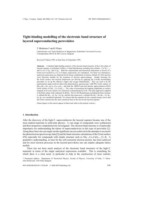
J. Phys.: Condens. Matter 12 (2000) 143–159. Printed in the UK PII: S0953-8984(00)02446-2Tight-binding modelling of the electronic band structure oflayered superconducting perovskitesT Mishonov† and E PenevLaboratorium voor Vaste-Stoffysica en Magnetisme, Katholieke Universiteit Leuven,Celestijnenlaan 200 D, B-3001 Leuven, BelgiumReceived 9 March 1999, in final form 22 September 1999Abstract. A detailed tight-binding analysis of the electron band structure of the CuO 2 plane oflayered cuprates is performed within a σ -band Hamiltonian including four orbitals—Cu 3d x 2 −y 2and Cu 4s, O 2p x and O 2p y . Both the experimental and theoretical indications in favour of aFermi level located in a Cu or O band, respectively, are considered. For these two alternatives,analytical expressions are obtained for the linear combination of atomic orbitals (LCAO) electronwave functions suitable for the treatment of electron superexchange. Simple formulae forthe Fermi surface and electron dispersions are derived by applying the Löwdin downfoldingprocedure to set up the effective copper and oxygen Hamiltonians. They are used to fit theexperimental angle-resolved ultraviolet photoelectron spectroscopy (ARUPS) Fermi surface ofPb 0.42 Bi 1.73 Sr 1.94 Ca 1.3 Cu 1.92 O 8+x and both the ARPES and local density approximation (LDA)Fermi surface of Nd 2−x Ce x CuO 4−δ . The value of presenting the hopping amplitudes as surfaceintegrals of ab initio atomic wave functions is demonstrated as well. The same approach is appliedto the RuO 2 plane of the ruthenate Sr 2 RuO 4 . The LCAO Hamiltonians including the three in-planeπ-orbitals Ru 4d xy ,O a 2p y ,O b 2p x and the four transverse π-orbitals Ru 4d zx ,Ru4d yz ,O a 2p z ,O b 2p z are considered separately. It is shown that the equation for the constant-energy curves andthe Fermi contours has the same canonical form as the one for the layered cuprates.(Some figures in this article appear in black and white in the printed version.)1. IntroductionAfter the discovery of the high-T c superconductors the layered cuprates became one of themost studied materials in solid-state physics. A vast range of compounds were synthesizedand their properties comprehensively investigated. The electron band structure is of particularimportance for understanding the nature of superconductivity in this type of perovskite [1].Along these lines one can single out the significant success achieved in the attempts to reconcilethe photoelectron spectroscopy data [2] and the band-structure calculations of the Fermi surface(FS) especially for compounds with simple structure such as Nd 2−x Ce x CuO 4−δ [3, 4]. Aqualitative understanding, at least for the self-consistent electron picture, has been achievedand for most electron processes in the layered perovskites one can employ adequate latticemodels.There has not been much analysis of the electronic band structures of the high-T cmaterials in terms of the single analytical expressions available. This is something forwhich there is a clear need, in particular to help in the construction of more realistic† Permanent address: Department of Theoretical Physics, Faculty of Physics, University of Sofia, 5 J BourchierBoulevard, 1164 Sofia, Bulgaria.0953-8984/00/020143+17$30.00 © 2000 IOP Publishing Ltd 143

144 T Mishonov and E Penevmany-body Hamiltonians. The aim of this paper is to analyse the common featuresin the electron band structure of the layered perovskites within the tight-binding (TB)method [5]. In the following we shall focus on the metallic (eventually superconducting)phase only, with the reservation that the antiferromagnetic correlations, especially in thedielectric phase, could substantially change the electron dispersions. It is shown thatthe linear combination of atomic orbitals (LCAO) approximation can be considered anadequate tool for analysing energy bands. Within the latter, exact analytic results areobtained for the constant-energy contours (CEC). These expressions are used to fit the FSof Nd 2−x Ce x CuO 4−δ [3], Pb 0.42 Bi 1.73 Sr 1.94 Ca 1.3 Cu 1.92 O 8+x [6], and Sr 2 RuO 4 [7] measuredin angle-resolved photoemission/angle-resolved ultraviolet spectroscopy (ARPES/ARUPS)experiments.In particular, by applying the Löwdin perturbative technique for the CuO 2 plane we givethe LCAO wave function of the states near the Fermi energy ɛ F . These states could be usefulin constructing the pairing theory for the CuO 2 plane. For the layered cuprates we find analternative concerning the Fermi-level location—Cu 3d x 2 −y 2 versus O 2pσ character of theconduction band. It is shown that analysis of extra spectroscopic data is needed in order forthis dilemma to be resolved. As regards the RuO 2 plane, the existence of three pockets of theFS unambiguously reveals the Ru 4dε character of the conduction bands [8, 9].To address the conduction bands in the layered perovskites we start from a commonHamiltonian including the basis of valence states O 2p and Ru 4dε, orCu3d x 2 −y2 and Cu 4s,respectively, for cuprates. Despite the equivalence of the crystal structures of Sr 2 RuO 4 [10]and La 2−x Ba x CuO 4 [11], the states in their conduction band(s) are, in some sense, complementary.In other words, for the CuO 2 plane the conduction band is of σ -character while forthe RuO 2 plane the conduction bands are determined by π-valence bonds. This is due to theseparation into σ - and π-part of the Hamiltonian H = H (σ ) + H (π) in the first approximation.The latter two Hamiltonians are studied separately.Accordingly, the paper is structured as follows. In section 2 we consider the generic H (4σ)Hamiltonian of the CuO 2 plane [12, 13] and H (π) = H (xy) + H (z) is then studied in section 3.The results of the comparison with the experimental data are summarized in section 4. Beforeembarking on a detailed analysis, however, we give an account of some clarifying issuesconcerning the applicability of the TB model and the band theory in general.1.1. Apology to the band theoryIt is well known that the electron band theory is a self-consistent treatment of the electronmotion in the crystal lattice. Even the classical three-body problem demonstrates stronglycorrelated solutions, so it is a priori unknown whether the self-consistent approximation isapplicable when describing the electronic structure of every new crystal. However, the oneparticleband picture is an indispensable stage in the complex study of materials. It is theanalysis of experimental data using a conceptually clear band theory that reveals nontrivialeffects: how strong the strongly correlated electronic effects are, whether it is possible to takeinto account the influence of some interaction-induced order parameter back into the electronicstructure etc. Therefore the comparison of the experiment with the band calculations is not anattempt, as sometimes thought, to hide the relevant issues—it is a tool to reveal interesting andnontrivial properties of the electronic structure.Many electron band calculations have been performed for the layered perovskites andresults were compared to data from ARPES experiments. The shape of the Fermi surfaceis probably the simplest test to check whether we are on the right track or whether someconceptually new theory should be used from the very beginning.

Modelling of layered superconducting perovskites 145The tight-binding interpolation of the electronic structure is often used for fitting theexperimental data. This is because the accuracy of that approximation is often higher than theuncertainties in the experiment. Moreover, the tight-binding method gives simple formulaewhich could be of use for experimentalists to see how far they can get with such a simplemindedapproach. The tight-binding parameters, however, have in a sense ‘their own life’independently of the ab initio calculations. These parameters can be fitted directly to theexperiment even when, for some reasons, the electron band calculations could give wrongpredictions. In this sense the tight-binding parameters are the appropriate intermediary betweenthe theory and experiment. As for the theory, establishing of reliable one-particle tight-bindingparameters is the preliminary step in constructing more realistic many-body Hamiltonians. Therole of the band theory is, thus, quite ambivalent: on one hand, it is the final ‘language’ usedin efforts towards understanding a broad variety of phenomena; on the other hand, it is thestarting point in developing realistic interaction Hamiltonians for sophisticated phenomenasuch as magnetism and superconductivity.The tight-binding method is the simplest one employed in the electron band calculationsand it is described in every textbook in solid-state physics; the layered perovskites are nowprobably the best-investigated materials and the Fermi surface is a fundamental notion in thephysics of metals. There is a consensus that the superconductivity of layered perovskites isrelated to electron processes in the CuO 2 and RuO 2 planes of these materials. It is not, however,fair to criticize a given study, employing the tight-binding method as an interpolation schemefor the first-principles calculations, for not thoroughly discussing the many-body effects. Thecriticism should rather be readdressed to the ab initio band calculations. An interpolationscheme cannot contain more information than the underlying theory. It is not erroneous ifsuch a scheme works with an accuracy high enough to adequately describe both the theory andexperiment.In view of the above, we find it very strange that there are no simple interpolation formulaefor the Fermi surfaces available in the literature and that experimental data are being publishedwithout an attempt towards simple interpretation. One of the aims of the present paper is tohelp interpret the experimental data by the tight-binding method as well as setting up notionsin the analysis of the ab initio calculations.2. Layered cuprates2.1. ModelThe CuO 2 plane appears as a common structural detail for all layered cuprates. Therefore,in order to retain the generality of the considerations, the electronic properties of the bareCuO 2 plane will be addressed without taking into account structural details such as dimpling,orthorhombic distortion, double planes, and surrounding chains. For the square unit cell withlattice constant a 0 a three-atom basis is assumed: {R Cu , R Ob , R Ob }={0,(a 0 /2,0), (0,a 0 /2)}.The unit cell is indexed by the vector n = (n x ,n y ), where n x ,n y = integer. Within such anidealized model the LCAO wave function spanned over the |Cu 3d x 2 −y 2〉, |Cu 4s〉, |O a 2p x 〉,|O b 2p y 〉 states reads asψ LCAO (r) = ∑ [X n ψ Oa 2p x(r − R Oa − a 0 n) + Y n ψ Ob 2p y(r − R Ob − a 0 n)n]+ S n ψ Cu 4s (r − R Cu − a 0 n) + D n ψ Cu 3d (r − R Cu − a 0 n)(2.1)where n = (D n ,S n ,X n ,Y n )is the tight-binding wave function in lattice representation.

+146 T Mishonov and E PenevThe neglect of the differential overlap leads to an LCAO Hamiltonian of the CuO 2 plane:H = ∑ {D † n [−t pd(−X n + X x−1,y + Y n − Y x,y−1 ) + ɛ d D n ]n+ S † n [−t sp(−X n + X x−1,y − Y n + Y x,y−1 ) + ɛ s S n ]+ X † n [−t pp(Y n − Y x+1,y − Y x,y−1 + Y x+1,y−1 )− t sp (−S n + S x+1,y ) − t pd (−D n + D x+1,y ) + ɛ p X n ]+ Y † n [−t pp(X n − X x−1,y − X x,y+1 + X x−1,y+1 )}− t sp (−S n + S x,y+1 ) − t pd (D n + D x,y+1 ) + ɛ p Y n ](2.2)where the components of n should be considered as being Fermi operators. ɛ d , ɛ s , andɛ p stand respectively for the Cu 3d x 2 −y2, Cu 4s and O 2pσ single-site energies. The directO a 2p x → O b 2p y exchange is denoted by t pp and similarly t sp and t pd denote the Cu 4s → O2pandO2p→Cu 3d x 2 −y 2 hoppings respectively. The sign rules for the hopping amplitudesare sketched in figure 1—the bonding orbitals enter the Hamiltonian with a negative sign.The latter follows directly from the surface integral approximation for the transfer amplitudes,given in appendix A.(x-1,y+1)(x,y+1)-+ - + ++ --+Cu4s(x-1,y)+(x,y)+(x+1,y)+ +---+ +-+ -O2p xO2p y--+ +-Cu3d x2-y2t pp -t ppt sp++----+ --t pdt pd+ -(x,y-1)-t sp(x+1,y-1)Figure 1. A schematic diagram of a CuO 2 plane (only orbitals relevant to the discussion aredepicted). The solid square represents the unit cell with respect to which the positions of theother cells are determined. The indices of the wave-function amplitudes involved in the LCAOHamiltonian (2.2) are given in brackets. The rules for determining the signs of the hopping integralst pd , t sp , and t pp are shown as well.For the Bloch states diagonalizing the Hamiltonian (2.2)⎛ ⎞⎛ ⎞D nD p⎜ S n ≡ n ⎟⎝ ⎠ = √ 1 ∑⎜ S p ⎟⎝X n N e iϕ a⎠ e ip·n (2.3)XppY n e iϕ bY p

Modelling of layered superconducting perovskites 147where N is the number of the unit cells; we use the same phases as in references [12, 13]:ϕ a = 1 2 (p x − π), ϕ b = 1 2 (p y − π). This equation describes the Fourier transformationbetween the coordinate representation n = (D n ,S n ,X n ,Y n ), with n being the cell index,and the momentum representation ψ p = (D p ,S p ,X p ,Y p )of the TB wave function (when usedas an index, the electron quasi-momentum vector is denoted by p). Hence, the Schrödingerequation i¯h d t ˆψ p,α = [ ˆψ p,α , H] ˆ for ψ p,α (t) = e −iɛt/¯h ψ p,α , with α being the spin index (↑, ↓)(suppressed hereafter), takes the form⎛⎞ ⎛ ⎞−ε d 0 t pd s X −t pd s Y D p(H p (4σ)⎜ 0 −ε−ɛ11)ψ p =s t sp s X t sp s Y ⎟ ⎜ S p ⎟⎝⎠ ⎝ ⎠ = 0 (2.4)t pd s X t sp s X −ε p −t pp s X s Y X p−t pd s Y t sp s Y −t pp s X s Y −ε p Y pwhereε d = ɛ − ɛ d ε s = ɛ − ɛ s ε p = ɛ − ɛ pands X = 2 sin( 1 2 p x) s Y = 2 sin( 1 2 p y)x = sin 2 ( 1 2 p x) y = sin 2 ( 1 2 p y)0 p x ,p y 2π.This 4σ -band Hamiltonian is generic for the layered cuprates; cf. reference [13]. We have alsoincluded the direct oxygen–oxygen exchange t pp dominated by the σ -amplitude. The secularequationdet(H p (4σ) −ɛ11) = Axy + B(x + y) + C = 0 (2.5)gives the spectrum and the canonical form of the CEC with energy-dependent coefficients:A(ɛ) = 16(4tpd 2 t sp 2 +2t2 sp t ppε d − 2tpd 2 t ppε s − tpp 2 ε dε s )B(ɛ) =−4ε p (t 2 sp ε d + t 2 pd ε s) (2.6)C(ɛ) = ε d ε s εp 2 .Hence, the explicit CEC equation reads asp y =±arcsin √ y if 0 y =− Bx+C 1. (2.7)Ax+BThis equation reproduces the rounded square-shaped FS, centred at the (π, π) point, inherentto all layered cuprates. The best fit is achieved when A, B, and C are considered as fittingparameters. Thus, for a CEC passing through the D = (p d ,p d ) and C = (p c ,π) referencepoints, as indicated in figure 2, the fitting coefficients (distinguished by the subscript ‘f ’) inthe canonical equationhave the formA f xy + B f (x + y) + C f = 0A f = 2x d − x c − 1 x d = sin 2 (p d /2)B f = x c − x 2 d x c = sin 2 (p c /2) (2.8)C f = x 2 d (x c +1)−2x c x dand the resulting LCAO Fermi contour is quite compatible with the LDA calculations forNd 2−x Ce x CuO 4−δ [4, 15]. Due to the simple shape of the FS, the curves just coincide. We

148 T Mishonov and E PenevZ,ΓΓ,ZCXDΓ,ZZ,ΓFigure 2. The LDA Fermi contour of Nd 2−x Ce x CuO 4−δ (dotted line) calculated by Yu andFreeman [4] (reproduced with the kind permission of the authors), and the LCAO fit (solid line)according to (2.5). The fitting procedure uses C and D as reference points.note also that the canonical equation (2.5) would formally correspond to the one-band TBHamiltonian of a 2D square lattice of the formɛ(p) =−2t(cos p x + cos p y ) +4t ′ cos p x cos p ywith strong energy dependence of the hopping parameters, where t ′ is the anti-bonding hoppingbetween the sites along the diagonal; cf. references [16, 17].2.2. Effective HamiltoniansStudies of the electronic structure of the layered cuprates have unambiguously proved theexistence of a large hole pocket—a rounded square centred at the (π, π) point. This observationis indicative for a Fermi level located in a single band of dominant Cu 3d x 2 −y 2 character. Toaddress this band and the related wave functions it is therefore convenient for an effective CuHamiltonian to be derived by Löwdin downfolding of the oxygen orbitals. This is equivalentto expressing the oxygen amplitudes from the third and fourth rows of (2.4):X = 1 [ (t pd s X 1+ t (ppsY)D 2 + t sp s X 1 − t ) ]ppsY2 Sη p ε p ε pwhereY = 1 η p[−t pd s Y(1+ t ppε ps 2 Xη p = ε p − t 2 ppε ps 2 X s2 Y)D + t sp s Y(1 − t ppε ps 2 X) ] (2.9)Sand substituting back into the first and the second rows of the same equation. Such adownfolding procedure results in the following energy-dependent copper Hamiltonian:⎛H Cu (ɛ) = ⎜⎝ɛ d + (2t pd) 2 (x + y + 8t )ppxyη p ε p(2t pd )(2t sp )η p(x − y)(2t pd )(2t sp )(x − y) ɛ s + (2t pd) 2 (x + y − 8t ppxyη p η p ε p⎞) ⎟⎠(2.10)

Modelling of layered superconducting perovskites 149which enters the effective Schrödinger equation( ) ( )D DH Cu = ɛ .S SThus, from (2.9) and (2.10) one can easily obtain an approximate expression for the eigenvectorcorresponding to a dominant Cu 3d x 2 −y 2 character. Taking D ≈ 1, in the lowest order withrespect to the hopping amplitudes t ll ′ one has⎛⎞⎛ ⎞D1|Cu 3d x 2 −y 2〉= ⎜S⎟(t sp t pd /ε s ε p )(sX 2 ⎝ ⎠≈⎜− s2 Y )⎟(2.11)X ⎝ (t pd /η p )s X ⎠Y−(t pd /η p )s Yi.e. |X| 2 + |Y | 2 + |S| 2 ≪|D| 2 ≈1. We note that within this Cu scenario the Fermi-levellocation and the CEC shape are not sensitive to the t pp -parameter. Therefore one can neglect theoxygen–oxygen hopping as was done, for example, by Andersen et al [12,13] (the importanceof the t pp -parameter has been considered by Markiewicz [14]) and the band structure of theHamiltonian (2.10) for the same set of energy parameters as used in reference [13] is shownin figure 3(a). In this case the FS can be fitted by its diagonal alone, i.e. using only D as areference point. Hence an equation for the Fermi energy isA(ɛ F )xd 2 +2B(ɛ F)x d + C(ɛ F ) = 0which yields ɛ F = 2.5 eV. As seen in figure 3(b), the deviation from the two-parameter fit,discussed in section 2.1, is almost vanishing, thus justifying the neglect of t pp and the using ofa one-parameter fit.107.5Energy (eV)52.50ΓYC- 2.5- 5Γ X M Γ(a)DΓ X Γ(b)Figure 3. (a) The electron band structure of the 4σ -band Hamiltonian generic for the CuO 2 planeobtained using the parameters from reference [13] and the Fermi level ɛ F = 2.5 eV fitted from theLDA calculation by Yu and Freeman [4]. (b) The LCAO Fermi contour (solid line) fitted to theLDA Fermi surface (dashed line) for Nd 2−x Ce x CuO 4−δ [4] using only D as a reference point. Thedeviation of the fit at the C point is negligible.However, despite the excellent agreement between the LDA calculations, the LCAO fit,and the ARPES data regarding the FS shape, the theoretically calculated conduction bandwidthw c in the layered cuprates is overestimated by a factor of 2 or even 3 [3]. Such a discrepancymay well point to some alternative interpretations of the available experimental data. In thefollowing section we shall consider the possibility for a Fermi level lying in an oxygen band.

150 T Mishonov and E Penev2.2.1. Oxygen scenario: the Abrikosov–Falkovsky model. There are currently variousindications in favour of O 2p character of the states near the Fermi level [18,19]. We considerthat these arguments cannot be a priori ignored. This is best seen if, following Abrikosov andFalkovsky [20], the experimental data are interpreted within an alternative oxygen scenario.Accordingly, the oxygen 2p level is assumed to lie above the Cu 3d x 2 −y 2 level, and theFermi level to fall into the upper oxygen band, ɛ d

Modelling of layered superconducting perovskites 151the energy surface defined by (2.17) is shown in figure 4(a). In figure 4(b) we have presenteda comparison between the ARPES data from reference [3] and the Fermi contour calculatedaccording to (2.17) for x = 0.15. Note that no fitting parameters are used and this contourshould be referred to as an ab initio calculation of the FS.(a)M(b)0024Γ2468θ10 12X1416182022x = 0.15ARPESCrossingΓ6810ϕ12YMY14YΓX16182022ΓXΓFigure 4. (a) The energy dispersion of the nonbonding oxygen band ɛ c (p), equation (2.17). Afew cuts through the energy surface, i.e. CEC, are presented together with the dispersion alongthe high-symmetry lines in the Brillouin zone. (b) The Fermi surface of Nd 2−x Ce x CuO 4−δ (solidline) determined from equation (2.17) for x = 0.15 (the shaded slice in panel (a)) and comparedwith experimental data (points with error bars) for the same value of x; after King et al [3]. θ andϕ denote the polar and azimuthal emission angles, respectively, measured in degrees. The emptydashed circles show k-space locations where ARPES experiments have been performed (cf. figure 2in reference [3]) and their diameter corresponds to 2 ◦ experimental resolution.The opposite limit case t eff ≫ B, i.e. τ ≫ 1, has been analysed in detail by Abrikosov andFalkovsky [20]. The conduction band dispersion rate ɛ c and the corresponding eigenvector ofthe Hamiltonian H O (2.13) now take the formɛ c ( p) = 4t eff (ɛ c ) √ xy (2.19)⎛⎞(t pd /ε d )(s X + s Y )|c〉 ≈√ 1(t sp /ε s )(s X − s Y )⎜⎟(2.20)2 ⎝ 1 ⎠−1provided that |D| 2 + |S| 2 ≪ |X| 2 + |Y| 2 ≈ 1. In other words, the last approximation,τ ≫ 1, corresponds to a pure oxygen model where only hoppings between oxygen ionsare taken into account. Clearly, this model is complementary to the copper scenario andis based on an effect completely neglected in its copper ‘counterpart’, where t pp ≡ 0.This limit case of the oxygen scenario suitably describes the ARUPS experimental data forPb 0.42 Bi 1.73 Sr 1.94 Ca 1.3 Cu 1.92 O 8+x [6]. The FS of the latter is fitted by its diagonal (the D point)according to the Abrikosov–Falkovsky relation (2.19) and the result is shown in figure 5.There exist a tremendous number of ARPES/ARUPS data for layered cuprates whichmakes the reviewing of all of those spectra impossible. To illustrate our TB model we havechosen data for the Pb substitution for Bi in Bi 2 Sr 2 CaCu 2 O 8 ; see figure 5. In this case the CuO 2planes are quite flat and the ARPES data are not distorted by structural details. When present,distortions were misinterpreted as a manifestation of strong antiferromagnetic correlations. We

152 T Mishonov and E Penev( a)() bXZΓYFigure 5. (a) The ARUPS Fermi surface of Pb 0.42 Bi 1.73 Sr 1.94 Ca 1.3 Cu 1.92 O 8+x given by Aebiet al [6]. (b) The LCAO fit to (a) according to the Abrikosov–Falkovsky model [20], using the Dreference point with p d = 0.171 × 2π.believe, however, that the experiment by Aebi et al [6] reveals the main feature of the CuO 2plane band structure—the large hole pocket found to be in agreement with the one-particleband calculations.Besides the good agreement between the theory and the experiment, regarding the FSshape, we should also point out the compatibility between the calculated and the experimentalconduction bandwidth. Indeed, within the Abrikosov–Falkovsky model [20], accordingto (2.19), one gets for the conduction bandwidth 0 ε c ( p) w c ≈ 4t pp , which coincideswith the value obtained from (2.17) provided that tpd 2 ≪ t pp(ɛ F − ɛ d ). The ab initio calculationof t pp as a surface integral (see appendix A), making use of atomic wave functions standardfor the quantum mechanical calculations, gives t pp ≈ 200–350 meV in different estimations.This range is in acceptable agreement with the experimental w c ≃ 1 eV [3]; within the LCAOmodel an exact analytic result for w c can be obtained from the equationw c = 4t pp +8tpd 2 /(w c − ɛ d ).We note also that the TB analysis allows the bands to be unambiguously classified withrespect to the atomic levels from which they arise. Within such terms, for the oxygen scenarioone can describe the metal → insulator transition as being the charge transferCu 1+ O 1 1 2 −2→ Cu 2+ O 2−2 .The possibility for monovalent copper Cu 1+ in the superconducting state is discussed, forexample, by Romberg et al [22].3. Conduction bands of the RuO 2 planeSr 2 RuO 4 is the first copper-free perovskite superconductor isostructural to the high-T ccuprates [10]. The layered ruthenates, just like the layered cuprates, are strongly anisotropicand in a first approximation the nature of the conduction band(s) can be understood by analysingthe bare RuO 2 plane. One should repeat the same steps as in the previous section, but nowhaving Ru instead of Cu and the Fermi level located in the metallic bands of Ru 4dπ character.To be specific, the conduction bands arise from the hybridization between the Ru 4d xy ,Ru4d yz ,Ru 4d zx and O a 2p y ,O b 2p x ,O a,b 2p z π-orbitals. The LCAO wave function spanned over the

Modelling of layered superconducting perovskites 153four orbitals perpendicular to the RuO 2 plane reads as (z)LCAO (r) = √ 1 ∑ ∑[D zx,n ψ Ru 4dzx (r − a 0 n) + D zy,n ψ Ru 4dzy (r − a 0 n)N p n]+e iϕ aZ a,n ψ Oa 2p z(r − R Oa − a 0 n) +e iϕ bZ b,n ψ Ob 2p z(r − R Ob − a 0 n) e ip·n .(3.1)Hence, the π-analogue of (2.4) takes the form⎛⎞ ⎛ ⎞−ε zx 0 t z,zx s X 0 D zx(H p(z)(z)− ɛ11)ψ p = ⎜ 0 −ε zy 0 t z,zy s Y ⎟ ⎜ D zy ⎟⎝⎠ ⎝ ⎠ = 0 (3.2)t z,zx s X 0 −ε za −t zz c X c Y Z a0 t z,zy s Y −t zz c X c Y −ε zb Z bwhereε zx = ɛ − ɛ zx ε za = ɛ − ɛ za c X = 2 cos(p x /2)(3.3)ε zy = ɛ − ɛ zy ε zb = ɛ − ɛ zb c Y = 2 cos(p y /2)and ɛ zx , ɛ zy , ɛ za , and ɛ zb are the single-site energies respectively for Ru 4d zx ,Ru4d zy ,O a 2p z ,and O b 2p z orbitals. t zz stands for the hopping between the latter two orbitals and, if anegligible orthorhombic distortion is assumed, the metal–oxygen π-hopping parameters areequal, t z,zy = t z,zx , and also ɛ z = ɛ za = ɛ zb . The phase factors e iϕ a,bin (3.1) are chosen incompliance with reference [13]; see equation (2.3).Identically, writing the LCAO wave function spanned over the three in-plane π-orbitalsRu 4d xy ,O a 2p y , and O b 2p x in the way in which (3.1) is designed, one has for the ‘in-plane’Schrödinger equation⎛⎞−ε xy t pdπ s X t pdπ s Y( ) Dxy(H p(xy) − ɛ11)ψ p (xy) = ⎝ t pdπ s X −ε ya t pp ′ s Xs Y⎠ Y a = 0 (3.4)t pdπ s Y t pp ′ s Xs Y −ε xbX bwhere t pdπ denotes the hopping Ru 4d xy → O a,b 2pπ and t pp ′ denotes the hopping O a 2p y →O b 2p x . The definitions for the other energy parameters are in analogy to (3.3) (for negligibleorthorhombic distortion, ɛ ya = ɛ xb ≠ ɛ z ). Thus, the π-Hamiltonian of the RuO 2 plane takesthe formH (π) =∑ψ p,α (z)† H p(z) ψ p,α (z) + ψ(xy)† p,α H p(xy) ψ p,α (xy) . (3.5)p,α=↑,↓In a previous paper [23] we derived the corresponding secular equations, and now we shalljust provide the final expressions in terms of the notation used here:det(H p (z,xy) − ɛ11) = A (z,xy) xy + B (z,xy) (x + y) + C (z,xy) = 0A (z) = 16(t 4 z,zx − t2 zz ε2 zx ) A(xy) = 32t ′ pp t 2 pdπ − 16ε xyt ′2ppB (z) =−16tzz 2 ε2 zx − 4t2 z,zx ε zxε z B (xy) =−tpdπ 2 ε ya(3.6)C (z) = εzx 2 (ε2 z − 16t zz 2 ) C(xy) = ε xy εya 2 .The three sheets of the Fermi surface in Sr 2 RuO 4 fitted to the ARPES data given by Luet al [7] are shown in figure 6(b). To determine the Hamiltonian parameters we have madeuse of the dispersion rate values at the high-symmetry points of the Brillouin zone. To thebest of our knowledge, the TB analysis of the Sr 2 RuO 4 band structure was first performed

154 T Mishonov and E Penev0- 1Energy (eV)- 2- 3- 4- 5XΓ Z X Γ(a)Γ(b)ZFigure 6. (a) The LCAO band structure of Sr 2 RuO 4 according to (3.5). The Fermi level (dashedline) crosses the three Ru 4dε bands of the RuO 2 plane. (b) The LCAO fit (solid lines) to theARPES data (circles) given by Lu et al [7]; cf. also reference [23].in reference [23] (subsequently, the latter results were reproduced in reference [25] withoutreferring to reference [23]). The RuO 2 -plane band structure resulting from the set of parameterst zz = t pp ′ = 0.3eV ε z =−2.3eV ε xy =−1.62 eV(3.7)t pdπ = t z,zx = 1eV ε zx =−1.3eV ε ya,xb =−2.62 eVis shown in figure 6(a). This fit is subject to the requirement of providing as good as possible adescription of the narrow energy interval around ɛ F , whereas the filled bands far below the Fermilevel match only qualitatively to the LDA calculations by Oguchi [8] and Singh [9]. In additionwe note that the de Haas–van Alphen (dHvA) measurements [26] of the Sr 2 RuO 4 FS differfrom the ARPES results [7]. Thus, fitting the dHvA data by using modified TB parametersis a natural refinement of the proposed model. We note that the diamond-shaped hole pocket,centred at the X point (see figure 6(b)), is very sensitive to the ‘game of parameters’. For thatband the Van Hove energy is fairly close to the Fermi energy. As a result, a minor change inthe parameters could drive a Van Hove transition transforming this hole pocket to an electronone, centred at the Ɣ point. Indeed, such a band configuration has been recently observed alsoin the ARPES revision of the Sr 2 RuO 4 Fermi surface [24]. This can be easily traced alreadyfrom the energy surfaces ɛ(p) calculated earlier in reference [23]. The comparison of theARPES data with TB energy surfaces could be a subject of a separate study.4. DiscussionThe LCAO analysis of the layered perovskites band structure, performed in the precedingsections, manifests a good compatibility with the experimental data and the band calculationsas well. Due to the strong anisotropy of these materials, their FS within a reasonable approximationare determined by the properties of the bare CuO 2 or RuO 2 planes.Despite these planes having identical crystal structures, their electronic structuresare quite different. While for the RuO 2 plane the Fermi level crosses metallic π-bands, the conduction band of the CuO 2 plane is described by the σ -Hamiltonian (2.4).The latter gives for the CuO 2 plane a large hole pocket centred at the (π, π) point.Its shape, if no additional sheets exist, is well described by the exact analyticresults within the LCAO model, equation (2.5), as found for Nd 2−x Ce x CuO 4−δ [3, 4]

Modelling of layered superconducting perovskites 155and Pb 0.42 Bi 1.73 Sr 1.94 Ca 1.3 Cu 1.92 O 8+x [6]. For a number of other cuprates, namelyYBa 2 Cu 3 O 7−δ [27], YBa 2 Cu 4 O 8 [21], Bi 2 Sr 2 CaCu 2 O 8 [28,29], Bi 2 Sr 2 CuO 6 [30], the infinitelayeredsuperconductor Sr 1−x Ca x CuO 2 [31], HgBa 2 Ca 2 Cu 3 O 8+δ [32], HgBa 2 CuO 4+δ [33],HgBa 2 Ca n−1 Cu n O 2n+2+δ [34], Tl 2 Ba 2 Ca n−1 Cu n O 4+2n [1], Sr 2 CuO 2 F 2 , Sr 2 CuO 2 Cl 2 , andCa 2 CuO 2 Cl 2 [35], this large hole pocket is easily identified. For all of the above compounds,however, its shape is usually deformed due to appearance of additional sheets of the Fermisurface originating from accessories of the crystal structure.As the most important implication for the CuO 2 plane we should point out the intrinsicalternative as regards the Fermi-level location (see section 2). It is commonly believed that thestates at the FS are of dominant Cu 3d x 2 −y2 character (see e.g. reference [13]). Nevertheless,the spectroscopic data for the FS can be equally well interpreted within the oxygen scenario,according to which the FS states are of dominant O 2pσ character. A number of indicationsexist in favour of the oxygen model and the importance of the t pp -hopping amplitude [14,18]:(i) O 1s → O 2p transitions observed in EELS experiments for the metallic phase of thelayered cuprates, which reveal an unfilled O 2p atomic shell;(ii) the oxygen scenario reproduces in a natural way the extended Van Hove singularityobserved in the ARPES experiments while the Cu scenario fails to describe it;(iii) the metal–insulator transition can be easily described;(iv) the width of the conduction band is directly related to the atomic wave functions.Some authors even ‘wager that the oxygen model will win’ [19] (if the oxygen scenario iscorroborated, due to the cancellation of the largest amplitude t sp the small hoppings t pd and t ppshould be properly evaluated eventually as surface integrals (see appendix A) and some bandcalculations may well need a revision). It would be quite valuable if a muffin-tin calculationfor the H + 2ion was performed and compared with the exact results when the hopping integralis comparatively small, of the order of the one that fits the ARPES data, t pp ∼ 200 meV. Wealso note that even the copper model gives an estimation for t pp closer to the experiment thanthe LDA calculations. The smallness of t pp within the oxygen scenario, on the other hand, isguaranteed by the nonbonding character of the conduction band. This scenario, therefore, caneasily display heavy-fermion behaviour, i.e. an effective masst pp →0m eff −→ hugeand a density of states (DOS) ∝ m eff ∝ 1/t pp (we note that no realistic band calculationsfor heavy-fermion systems can be performed without employing the asymptotic methods fromatomic physics). It is also instructive to compare the TB analyses of heavy-fermion systems andlayered cuprates. The alternatives for the Fermi-level location (metallic versus oxygen band)exist for the cubic bismuthates as well [43,44]. When the Fermi level falls into heavy-fermionoxygen bands, one of the isoenergy surfaces is a rounded cube [43]. Indeed, such an isoenergysurface has been recently confirmed by the LMTO method applied to Ba 0.6 K 0.4 BiO 3 [45].Due to the equally good fit of the results for the FS of the layered cuprates within thetwo models, we can infer that at present any final judgment about this alternative wouldbe premature. Thus far we consider that the oxygen model should be taken into accountin the interpretation of the experimental data. Moreover, the angular dependence of thesuperconducting order parameter ( p) ∝ cos(p x ) − cos(p y ) is readily derived within thestandard BCS treatment of the oxygen–oxygen superexchange [36]. Analysis of some extraspectroscopic data by means of different models would finally resolve this dilemma. Thiscannot be done within the framework of the TB method. A coherent picture requires a thoroughstudy, where the TB model is just a useful tool for testing the properties of a given solution.

156 T Mishonov and E PenevUp to now, the applicability of the LCAO approximation to the electron structure ofthe layered cuprates can be considered as being proved. The basis function of the LCAOHamiltonian can be included in a realistic one-electron part of the lattice Hamiltonians forthe layered perovskites. This is an indispensable step preceding the inclusion of the electron–electron superexchange, electron–phonon interaction or any other kind of interaction betweenconducting electrons.AcknowledgmentsThe authors are especially grateful to P Aebi for being so kind as to provide them with extradetails on ARUPS spectra as well as for correspondence on this topic. We are much indebted toJ Indekeu for hospitality and the good atmosphere during completion of this work, and wouldlike to thank R Danev, I Genchev and R Koleva for collaboration in the initial stages of thisstudy. This paper was partially supported by the Bulgarian NSF No 627/1996, the BelgianDWTC, the Flemish Government Programme VIS/97/01, the IUAP, and the GOA.Appendix A. Calculation of the O–O hopping amplitude by the surface integral methodFrom quantum mechanics [37] it is well known that the usual quantum chemistry calculationof the hopping integrals as matrix elements of the single-particle Hamiltonian does not workwhen the overlap between the atomic functions is too weak. If the hopping integrals aremuch smaller than the detachment energy, they should be calculated as surface integrals using(eventually distorted by the polarization) atomic wave functions.Such an approach has been applied by Landau and Lifshitz [37] and Herring and Flicker[38] to the simple H + 2problem and now the asymptotic methods are well developed in thephysics of atomic collisions [39]. On the basis of the above problem one can easily verifythat the atomic sphere muffin-tin approximation of the Coulomb potentials usual in condensedmatter physics undergoes fiasco when the hopping integrals are of the order of 200–300 meV.Therefore, the factor 2–3 misfit for a single-electron problem cannot be ascribed to the strongcorrelationeffects, renormalizations, and other incantations which are often used to accountfor the discrepancy between the experimental bandwidth and the LDA calculations.Usually, condensed matter physics does not need asymptotically accurate methods forcalculation of hopping integrals, which leads to zero overlap between the muffin-tin andasymptotic methods. However, for the perovskites the largest hopping t sp cancels in theexpression for the upper oxygen band ɛ c ( p). Thus, small hoppings become essential, buthaving no influence on the other bands, and the necessity of taking into account t pp is oftopological nature.Following the calculations for H + 2 [37], in a simplified picture of two oxygen atoms O a,O bseparated by distance d = ( √ 2/2)a 0 the surface integral method gives for the oxygen–oxygenexchange the following explicit expression:∫ ∫t pp = ¯h2 (ψ Oa ∂ z ψ Ob − ψ Ob ∂ z ψ Oa ) dx dy (A.1)2m Swhere the integral is taken over the surface S bisecting d, and m is the electron mass. Thust pp = t pp (ξ) is a function of ξ = κ|R Oa − R Ob | with κ 2 /2 being the oxygen detachment energyin atomic units and the detailed derivation of (A.1) can be found, for example, in reference [39].We note that the derivation of t pp (ξ) imposes no restrictions on the basis set {ψ} used.Hence we choose {ψ Oa,b } to be the simplest minimal (MINI) basis used [40], for example, inthe GAMESS package for doing ab initio electronic structure calculations [41]. The MINI

Modelling of layered superconducting perovskites 157bases are three Gaussian expansions of each atomic orbital. The exponents and contractioncoefficients are optimized for each element, and the s and p exponents are not constrained tobe equal.Accordingly, the oxygen 2p radial wave function R 2p (r) is replaced by a Gaussian expansionR (G)2p(r) and has the form3∑R (G)2p(ζ, r) =i=1C 2p,i g 2p,i (ζ 2p,i , r)(A.2)where g 2p (ζ, r) = A 2p,i e −ζ 2p,ir 2 , and the coefficients for oxygen are given in table A1. It isthen normalized to unity according to∫ ∞0R (G)22pr 2 dr = 1.Table A1. Coefficients for the oxygen 2p wave function in the MINI basis [41].i C 2p,i A 2p,i ζ 2p,i1 8.2741400 2.485782 0.7085202 1.1715463 1.333720 0.4765943 0.3030130 0.263299 0.130440By multiplying with the corresponding cubic harmonic, the oxygen wave functions arebrought into the form√ {3ψ Oa (r a ) = R (G)2p (ζ, r x a ra = r − R Oaa)(A.3)4π r a r a =|r a |and analogously for ψ Ob (r − R Ob ). Substituting (A.3) in (A.1) we gett (MINI)pp= 340 meV.In reference [42] the same integral has been calculated with {ψ} being the asymptotic wavefunctions [39] appropriately tailored to the MINI basis at their outermost inflection pointsr (i) , i.e.⎧⎪⎨ R (G)2pR 2p (r) =√ (r) r r(i)2κ(A.4)⎪⎩ A e −κr r r (i)rwith κ = 0.329 and A = 0.5. The value obtained ist (asymp)pp= 210 meVwhich is found to be in good agreement with that fitted from the ARPES experiment withinthe oxygen scenario. A similar calculation gives, for example, for the t pd - and t sp -hoppingst (MINI)pd= 580 meV t sp(MINI) ∼ 2.5eV.Note added in proof. In a very recent paper by Campuzano et al [46] the ARPES Fermi surface of pureBi 2 Sr 2 CaCu 2 O 8+δ has been presented in the inset of their figure 1(a). This experimental finding is in excellentagreement with our tight-binding fit to the Fermi surface of Pb 0.42 Bi 1.73 Sr 1.94 Ca 1.3 Cu 1.92 O 8+x , studied by Schwallerand co-workers in reference [6], given in figure 5 of the present paper. The remarkable coincidence of the Fermisurfaces of these two compounds is a nice confirmation that Pb substitution for Bi is irrelevant for the band structureof the CuO 2 plane and the Fermi surface of the latter is therefore revealed to be a common feature.

158 T Mishonov and E PenevReferences[1] Pickett W E 1989 Rev. Mod. Phys. 61 433[2] Shen Z-X and Dessau D S 1995 Phys. Rep. 253 1Lynch D W and Olson C G 1999 Photoemission Studies of High-Temperature Superconductors (Cambridge:Cambridge University Press)[3] King D M, Shen Z-X, Dessau D S, Wells B O, Spicer W E, Arko A J, Marshall D S, DiCarlo J, Loeser A G,Park C H, Ratner E R, Peng J L, Li Z Y and Greene R L 1993 Phys. Rev. Lett. 70 3159[4] Yu J and Freeman A J 1991 Proc. Conf. on Advances in Materials Science and Applications of High TemperatureSuperconductors (NASA Conf. Publication 3100) (Greenbelt, MD, 2–6 April 1990) ed L H Bennett et al(Washington, DC: US Government Printing Office) pp 365–71[5] For a nice review on the tight-binding method seeGoringe C M, Bowler D R and Hernández E 1997 Rep. Prog. Phys. 60 1447Eschrig H 1989 Optimized LCAO Method and the Electronic Structure of Extended Systems (Berlin: Springer)Bullett D W 1980 Springer Series in Solid State Physics vol 35 (Berlin: Springer) p 129[6] Aebi P, Osterwalder J, Schwaller P, Schlapbach L, Shimoda M, Mochiku T and Kadowaki K 1994 Phys. Rev.Lett. 72 2757Aebi P, Osterwalder J, Schwaller P, Schlapbach L, Shimoda M, Mochiku T and Kadowaki K 1995 Phys. Rev.Lett. 74 1886Osterwalder J, Aebi P, Schwaller P, Schlapbach L, Shimoda M, Mochiku T and Kadowaki K 1995 Appl. Phys.A 60 247Aebi P, Osterwalder J, Schwaller P, Schlapbach L, Shimoda M, Mochiku T, Kadowaki K, Berger H and Lévy F1994 Physica C 235–240 949[7] Lu D H, Schmidt M, Cummins T R, Schuppler S, Lichtenberg F and Bednorz J G 1996 Phys. Rev. Lett. 76 4845[8] Oguchi T 1995 Phys. Rev. B 51 1385[9] Singh D J 1995 Phys. Rev. B 52 1358[10] Maeno Y, Hashimoto H, Yoshida K, Nishizaki S, Fujita T, Bednorz J G and Lichtenberg F 1994 Nature 372 532[11] Bednorz J G and Müller K A 1986 Z. Phys. B 64 189[12] Andersen O K, Jepsen O, Liechtenstein A I and Mazin I I 1994 Phys. Rev. B 49 4145Andersen O K, Savrazov S Y, Jepsen O and Liechtenstein A I 1996 J. Low Temp. Phys. 105 285 and referencestherein[13] Andersen O K, Liechtenstein A I, Jepsen O and Paulsen F 1995 J. Phys. Chem. Solids 56 1573[14] Markiewicz R S 1997 J. Phys. Chem. Solids 58 1179 (section 5)[15] Massidda S, Hamada N, Yu J and Freeman A J 1989 Physica C 157 571[16] Yu J and Freeman A J 1991 J. Phys. Chem. Solids 52 1351[17] Radtke R J, Levin K, Schüttler H-B and Norman M R 1993 Phys. Rev. B 48 15 957Radtke R J and Norman M R 1994 Phys. Rev. B 50 9554[18] Stechel E B and Jennison D R 1988 Phys. Rev. B 38 4632Stechel E B and Jennison D R 1988 Phys. Rev. B 38 8873Takahashi T, Matsuyama H, Katayama-Yoshida H, Okabe Y, Hosoya S, Seki K, Fujimoto H, Sato M andInokuchi H 1988 Nature 334 691Tanaka M, Takahashi T, Katayama-Yoshida H, Yamazaki S, Fujinami M, Okabe Y, Mizutani W, Ono M andKajimura K 1989 Nature 339 691Takahashi T 1989 Strong Correlation and Superconductivity (Springer Series in Solid State Sciences vol 89) edA Fukuyama et al (Berlin: Springer) p 311[19] Blackstead H A and Dow J 1997 Physica C 282–287 1513[20] Abrikosov A A and Falkovsky L A 1990 Physica C 168 556[21] Gofron K, Campuzano J C, Abrikosov A A, Lindroos M, Bansil A, Ding H, Koelling D and Dobrovski B 1994Phys. Rev. Lett. 73 3302[22] Romberg H, Nücker N, Alexander M, Fink J, Hahn D, Zetterer T, Otto H H and Renk K F 1990 Phys. Rev. B 412609Nücker N, Romberg H, Alexander M and Fink J 1999 Electronic structure studies of high-T c cuprate superconductorsby electron energy-loss spectroscopy Studies of High Temperature Superconductors vol 6, edA Narlikar (New York: Nova Science)[23] Mishonov T M, Genchev I N, Koleva R K and Penev E 1996 J. Low Temp. Phys. 105 1611Mishonov T M, Genchev I N, Koleva R K and Penev E 1996 Czech. J. Phys. Suppl. S2 46 953[24] Puchkov A V, Shen Z-X, Kimura T and Tokura Y 1998 Phys. Rev. B 58 R13 322[25] Noce C and Cuoco M 1999 Phys. Rev. B 59 2659

Modelling of layered superconducting perovskites 159[26] Makenzie A P, Julian S R, Diver A J, McMullan G J, Ray M P, Lonzarich G G, Maeno Y, Nishizaki S andFujita T 1996 Phys. Rev. Lett. 76 3786[27] Yu J, Massidda S, Freeman A J and Koelling D D 1987 Phys. Lett. A 122 203[28] Marshall D S, Dessau D S, King D M, Park C-H, Matsuura A Y, Shen Z-X, Spicer W E, Eckstein JNandBozovic I 1995 Phys. Rev. B 52 12 548Ding H, Bellman A F, Campuzano J S, Randeria M, Norman M R, Yokoya T, Takahashi T, Katayama-Yoshida H,Mochiku T, Kadowaki K, Jennings J and Brivio G P 1996 Phys. Rev. Lett. 76 1533[29] Massidda S, Yu Jaejun and Freeman A J 1988 Physica C 158 251[30] Singh D J and Pickett W E 1995 Phys. Rev. B 51 3128[31] Novikov D L, Gubanov V A and Freeman A J 1993 Physica C 210 301[32] Singh D J and Pickett W E 1994 Physica C 233 237Singh D J and Pickett W E 1994 Phys. Rev. Lett. 73 476[33] Novikov D L and Freeman A J 1993 Physica C 212 233[34] Novikov D L and Freeman A J 1993 Physica C 216 273[35] Novikov D L, Freeman A J and Jorgensen J D 1995 Phys. Rev. B 51 6675[36] Mishonov T M and Donkov A A 1996 Czech. J. Phys. Suppl. S2 46 1051Mishonov T M, Donkov A A, Koleva R K and Penev E S 1997 Bulgarian J. Phys. 24 114Mishonov T M and Donkov A A 1997 J. Low Temp. Phys. 107 541[37] Landau L D and Lifshitz E M 1974 Quantum Mechanics (Theoretical Physics vol 3) (Moscow: Nauka) (inRussian)[38] Herring C and Flicker M 1964 Phys. Rev. 134 A362[39] Smirnov B M 1973 Asymptotic Methods in the Theory of Atomic Collisions (Moscow: Energoatomizdat) (inRussian)[40] Huzinaga S, Andzelm J, Klobukowski M, Radzio-Andzelm E, Sakai Y and Tatewaki H 1984 Gaussian BasisSets for Molecular Calculations (Amsterdam: Elsevier)[41] Schmidt M W, Baldrige K K, Boatz J A, Jensen J H, Koseki S, Gordon M S, Nguyen K A, Windus T L, Elbert ST 1992 QCPE Bull. 10 52[42] Mishonov T M, Koleva R K, Genchev I N and Penev E 1996 Czech. J. Phys. Suppl. S5 46 2645[43] Mishonov T, Genchev I, Koleva R and Penev E 1997 Superlatt. Microstruct. 21 471[44] Mishonov T, Genchev I and Penev E 1997 Superlatt. Microstruct. 21 477[45] Meregalli V and Savrazov Y 1998 Phys. Rev. B 57 14 453[46] Campuzano J C et al 1999 Phys. Rev. Lett. 83 3709