ANCOVA Example - categorical covariate

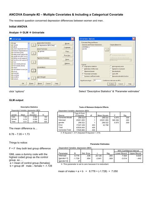
ANCOVA Example #2 – Multiple Covariates & Including a Categorical CovariateThe research question concerned depression differences between women and men.Initial ANOVAAnalyze GLM Univariateclick “options”Select “Descriptive Statistics” & “Parameter estimates”GLM outputDescriptive StatisticsDependent Variable: depression (BDI)Std.gender Mean Deviation Nmale 7.05 5.992 180female 8.78 6.950 225Total 8.01 6.590 405The mean difference is…8.78 – 7.05 = 1.73Tests of Between-Subjects EffectsDependent Variable: depression (BDI)Type III SumSourceof Squares df Mean Square F Sig.Corrected Model 298.522 a 1 298.522 6.975 .009Intercept25051.855 1 25051.855 585.356 .000gender298.522 1 298.522 6.975 .009Error17247.439 403 42.798Total43530.000 405Corrected Total 17545.960 404a. R Squared = .017 (Adjusted R Squared = .015)Things to notice:F = t² they both test group differenceGML uses a dummy code with thehighest coded group as the controlgroup, so …a = mean of control group (females)b = group dif male – female = -1.728Dependent Variable: depression (BDI)ParameterIntercept[gender=1][gender=2]Parameter Estimates95% Confidence IntervalB Std. Error t Sig. Lower Bound Upper Bound8.778 .436 20.126 .000 7.920 9.635-1.728 .654 -2.641 .009 -3.014 -.4420 a . . . . .a. This parameter is set to zero because it is redundant.mean of males = a + b = 8.778 + (-1.728) = 7.050

ANCOVA with Multiple CovariatesAnalyze GLM Univariate“Covariates” can be any quantitative, binary or codedvariable.Adding variables to the “Covariates” window will create aANCOVA.Moving the “IV” into the “Display Means for” window willgive use the “corrected mean” for each condition of thevariable.GLM outtputDescriptive StatisticsDependent Variable: depression (BDI)Std.gender Mean Deviation Nmale 7.05 5.992 180female 8.78 6.950 225Total 8.01 6.590 405agelonelinesstotal social supportDescriptive StatisticsStd.Mean Deviation28.48 10.88537.21 11.3775.6233 1.18204Tests of Between-Subjects EffectsDependent Variable: depression (BDI)Type III SumSourceof Squares df Mean Square F Sig.Corrected Model 6281.245 a 4 1570.311 55.760 .000Intercept40.821 1 40.821 1.450 .229age930.640 1 930.640 33.046 .000ruls2982.872 1 2982.872 105.919 .000tss74.807 1 74.807 2.656 .104gender580.881 1 580.881 20.627 .000Error11264.715 400 28.162Total43530.000 405Corrected Total 17545.960 404a. R Squared = .358 (Adjusted R Squared = .352)genderDependent Variable: depression (BDI)gendermalefemale95% Confidence IntervalMean Std. Error Lower Bound Upper Bound6.642 a .400 5.855 7.4299.104 a .357 8.402 9.806a. Covariates appearing in the model are evaluated at thefollowing values: age = 28.48, loneliness = 37.21, totalsocial support = 5.6233.Dependent Variable: depression (BDI)ParameterInterceptagerulstss[gender=1][gender=2]Parameter Estimates95% Confidence IntervalB Std. Error t Sig. Lower Bound Upper Bound4.340 2.633 1.649 .100 -.835 9.515-.145 .025 -5.749 .000 -.195 -.096.311 .030 10.292 .000 .251 .370-.473 .290 -1.630 .104 -1.043 .097-2.462 .542 -4.542 .000 -3.528 -1.3960 a . . . . .a. This parameter is set to zero because it is redundant.Again, the regression weight for gender is the same as the corrected mean difference. b = the mean difference “holding the value of the covariates constant at their means”Because there are no interactions (i.e.,making the regression homogeneity assumption) the regression weights tell andtest the slope of each quantitative covariate for both group, correcting for the other variables in the model.

ANCOVA with Multiple Covariates Including a Categorical CovariateIf we put more than one variable into the “Fixed Factors”window, we will obtain a factorial analysis.If we want an ANCOVA instead of a factorial, we canspecify that we want a “main effects model” -- as shownbelow on the left.We would also want to get the corrected group means foreach of the categorical variables (gender and maritalstatus) that go with the ANCOVA F-tests for these variablesand regression parameters that tell about the correctedeffects of the quantitative variables (age, ruls,TSS) that gowith the ANCOVA F-tests for these variables – as shownbelow on the right.

GLM outputDescriptive StatisticsDependent Variable: depression (BDI)gender marital MeanStd.Deviation Nmale single7.25 5.673 122married 6.11 6.699 47divorced 8.91 6.188 11Total7.05 5.992 180female single 10.04 8.110 120married 6.89 4.571 74divorced 8.39 5.800 31Total8.78 6.950 225Total single8.63 7.113 242married 6.59 5.483 121divorced 8.52 5.832 42Total8.01 6.590 405The “raw” means are above and the “corrected” means are on theright.1. genderDependent Variable: depression (BDI)gendermalefemale95% Confidence IntervalMean Std. Error Lower Bound Upper Bound6.547 a .514 5.535 7.5588.991 a .455 8.097 9.885a. Covariates appearing in the model are evaluated at thefollowing values: age = 28.48, loneliness = 37.21, totalsocial support = 5.6233.2. maritalDependent Variable: depression (BDI)maritalsinglemarrieddivorced95% Confidence IntervalMean Std. Error Lower Bound Upper Bound8.222 a .452 7.333 9.1117.160 a .636 5.910 8.4117.924 a .981 5.995 9.854a. Covariates appearing in the model are evaluated at thefollowing values: age = 28.48, loneliness = 37.21, total socialsupport = 5.6233.Dependent Variable: depression (BDI)SourceCorrected ModelInterceptgendermaritalagerulstssErrorTotalCorrected TotalTests of Between-Subjects EffectsType III Sumof Squares df Mean Square F Sig.6328.474 a 6 1054.746 37.423 .00011.239 1 11.239 .399 .528568.049 1 568.049 20.155 .00047.229 2 23.614 .838 .433208.332 1 208.332 7.392 .0072981.050 1 2981.050 105.769 .00057.999 1 57.999 2.058 .15211217.487 398 28.18543530.000 40517545.960 404a. R Squared = .361 (Adjusted R Squared = .351)Notice again that the F-tests and t-tests tellthe same story, except for Marital statusThe F-test is a test of the “marital effect”,while the t-tests of the individual dummycodes test specific pairwise comparisons.If either of the dummy codes (pairwisecomparisons) are significant, then the F-testof that k-group effect will be significant.Dependent Variable: depression (BDI)ParameterIntercept[gender=1][gender=2][marital=1][marital=2][marital=3]agerulstssParameter Estimates95% Confidence IntervalB Std. Error t Sig. Lower Bound Upper Bound3.207 3.150 1.018 .309 -2.985 9.399-2.445 .545 -4.489 .000 -3.515 -1.3740 a . . . . ..298 1.213 .246 .806 -2.087 2.683-.764 .969 -.789 .431 -2.669 1.1410 a . . . . .-.114 .042 -2.719 .007 -.197 -.032.311 .030 10.284 .000 .251 .370-.421 .293 -1.435 .152 -.997 .156a. This parameter is set to zero because it is redundant.Note: It is possible to have a significant F,without either of the dummy-code t-tests tobe significant if the comparison grouphappens to be the middle-value mean, thenit might be different from neither the groupwith the higher nor the lower mean, whilethose groups are different from each otherBecause there are no interactions(i.e.,making the regression homogeneityassumption) the regression weights tell andtest the slope of each quantitative covariatefor both groups, correcting for the othervariables in the model.