Lecture notes - Institut für Mathematik - TU Berlin

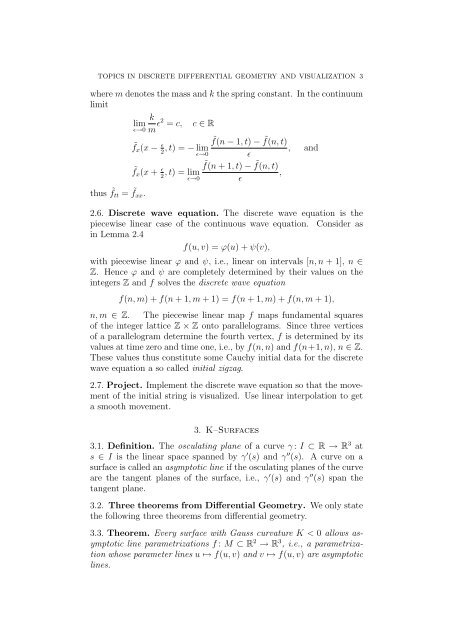
TOPICS IN DISCRETE DIFFERENTIAL GEOMETRY AND VISUALIZATION 3where m denotes the mass and k the spring constant. In the continuumlimitklimɛ→0 m ɛ2 = c, c ∈ Rthus ˜f tt = ˜f xx .˜f x (x − ɛ , t) = − lim2 ɛ→0˜f x (x + ɛ , t) = lim2 ɛ→0˜f(n − 1, t) − ˜f(n, t), andɛ˜f(n + 1, t) − ˜f(n, t),ɛ2.6. Discrete wave equation. The discrete wave equation is thepiecewise linear case of the continuous wave equation. Consider asin Lemma 2.4f(u, v) = ϕ(u) + ψ(v),with piecewise linear ϕ and ψ, i.e., linear on intervals [n, n + 1], n ∈Z. Hence ϕ and ψ are completely determined by their values on theintegers Z and f solves the discrete wave equationf(n, m) + f(n + 1, m + 1) = f(n + 1, m) + f(n, m + 1),n, m ∈ Z. The piecewise linear map f maps fundamental squaresof the integer lattice Z × Z onto parallelograms. Since three verticesof a parallelogram determine the fourth vertex, f is determined by itsvalues at time zero and time one, i.e., by f(n, n) and f(n+1, n), n ∈ Z.These values thus constitute some Cauchy initial data for the discretewave equation a so called initial zigzag.2.7. Project. Implement the discrete wave equation so that the movementof the initial string is visualized. Use linear interpolation to geta smooth movement.3. K–Surfaces3.1. Definition. The osculating plane of a curve γ : I ⊂ R → R 3 ats ∈ I is the linear space spanned by γ ′ (s) and γ ′′ (s). A curve on asurface is called an asymptotic line if the osculating planes of the curveare the tangent planes of the surface, i.e., γ ′ (s) and γ ′′ (s) span thetangent plane.3.2. Three theorems from Differential Geometry. We only statethe following three theorems from differential geometry.3.3. Theorem. Every surface with Gauss curvature K < 0 allows asymptoticline parametrizations f : M ⊂ R 2 → R 3 , i.e., a parametrizationwhose parameter lines u ↦→ f(u, v) and v ↦→ f(u, v) are asymptoticlines.