Split-Plot ANOVA Neuroscience 9506 Statistics for ... - Paul Gribble

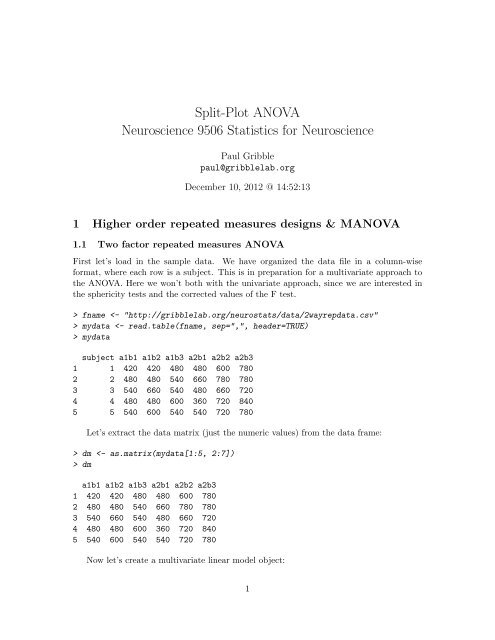
Split-Plot ANOVANeuroscience 9506 Statistics for NeurosciencePaul Gribblepaul@gribblelab.orgDecember 10, 2012 @ 14:52:131 Higher order repeated measures designs & MANOVA1.1 Two factor repeated measures ANOVAFirst let’s load in the sample data. We have organized the data file in a column-wiseformat, where each row is a subject. This is in preparation for a multivariate approach tothe ANOVA. Here we won’t both with the univariate approach, since we are interested inthe sphericity tests and the corrected values of the F test.> fname mydata mydatasubject a1b1 a1b2 a1b3 a2b1 a2b2 a2b31 1 420 420 480 480 600 7802 2 480 480 540 660 780 7803 3 540 660 540 480 660 7204 4 480 480 600 360 720 8405 5 540 600 540 540 720 780Let’s extract the data matrix (just the numeric values) from the data frame:> dm dma1b1 a1b2 a1b3 a2b1 a2b2 a2b31 420 420 480 480 600 7802 480 480 540 660 780 7803 540 660 540 480 660 7204 480 480 600 360 720 8405 540 600 540 540 720 780Now let’s create a multivariate linear model object:1

Neurostats Using R 1 Higher order repeated measures designs & MANOVA> mlm1 library(car)> af bf myfac myfacfactorA factorB1 a1 b12 a1 b23 a1 b34 a2 b15 a2 b26 a2 b3Now we will define the anova using Anova():> mlm1.aov summary(mlm1.aov, multivariate=FALSE)Univariate Type III Repeated-Measures ANOVA Assuming SphericitySS num Df Error SS den Df F Pr(>F)(Intercept) 10443000 1 33600 4 1243.214 3.861e-06 ***factorA 147000 1 33600 4 17.500 0.013881 *factorB 138480 2 39120 8 14.159 0.002354 **factorA:factorB 67920 2 23280 8 11.670 0.004246 **---Signif. codes: 0 ‘***’ 0.001 ‘**’ 0.01 ‘*’ 0.05 ‘.’ 0.1 ‘ ’ 1Mauchly Tests for SphericityTest statistic p-valuefactorB 0.76047 0.66317factorA:factorB 0.96131 0.94254Greenhouse-Geisser and Huynh-Feldt Corrections1 If you don’t have the car package installed, just type install.packages("car") and R will downloadit and install it.2

Neurostats Using R 1 Higher order repeated measures designs & MANOVAfor Departure from SphericityGG eps Pr(>F[GG])factorB 0.80676 0.005291 **factorA:factorB 0.96275 0.004857 **---Signif. codes: 0 ‘***’ 0.001 ‘**’ 0.01 ‘*’ 0.05 ‘.’ 0.1 ‘ ’ 1HF eps Pr(>F[HF])factorB 1.2712 0.002354 **factorA:factorB 1.8384 0.004246 **---Signif. codes: 0 ‘***’ 0.001 ‘**’ 0.01 ‘*’ 0.05 ‘.’ 0.1 ‘ ’ 1Note how the formula FactorA*FactorB uses the same names as in the myfac dataframe we defined.The first part of the output lists the omnibus F tests for the main effects and theinteraction effect. We then see the Mauchly tests of sphericity. We see tests for the maineffect of factorB, and the factorA:factorB interaction effect. We don’t see a test of the maineffect of factorA, because in this case, factorA has only two levels ... and so there is novariances of differences-between-groups... since there are only two levels, there is only asingle variance of differences (between the two levels). We then see Greenhouse-Geisser andHuynh-Felft corrections.1.1.1 Simple main effectsThe factorA:factorB interaction is significant, so we want to conduct so-called simple maineffects analyses. This would be testing the effects of one factor (e.g. factorB), separatelywithin each level of factorA (or vice-versa). In a between-subjects two-factor ANOVA, simplemain effects are evaluated by doing separate one-way ANOVAs, but using the MSerrorterm from the overall two-factor analysis as the error term. For within-subjects designsit’s probably better to use separate error terms for each analysis, since the sphericity assumptionis likely not true, and repeated measures ANOVA Is sensitive (more so thanbetween-subjects ANOVA) to violations of the sphericity assumption. Therefore we can infact literally run separate single-factor repeated measures ANOVAs, with one factor, withinlevels of the other factor.1.1.2 Pairwise tests & linear contrastsThe approach for computing linear contrasts (including pairwise tests) is the same as fora single-factor repeated measures design. We can either compute F ratios by taking theappropriate MSerr term from the ANOVA output (this approach assumes sphericity), or wecan simple compute differences scores and perform t-tests (this doesn’t assume sphericity).Correcting for Type-I error is up to you — you could use a Bonferroni adjustment, orcompute Tukey probabilities, etc.3

Neurostats Using R 1 Higher order repeated measures designs & MANOVA1.2 Split plot designsA split plot design is a mixed design in which there are some repeated measures factor(s)and some between-subjects factor(s). Let’s load in some sample data for a study with onerepeated measures and one between subjects factor:> fname mdata mdatasubject a1 a2 a3 gender1 1 420 420 480 f2 2 480 480 540 f3 3 540 660 540 f4 4 480 480 600 f5 5 540 600 540 f6 6 439 434 495 m7 7 497 497 553 m8 8 555 675 553 m9 9 492 496 615 m10 10 555 617 555 mWe have three levels of a repeated measures factor (a1, a2, a3) and two levels of abetween-subjects factor, gender (m,f), and 10 subjects.First as before we extract the data corresponding to the dependent variable from thedata frame:> dm dma1 a2 a31 420 420 4802 480 480 5403 540 660 5404 480 480 6005 540 600 5406 439 434 4957 497 497 5538 555 675 5539 492 496 61510 555 617 555Then we formulate our multivariate model:> mlm

Neurostats Using R 1 Higher order repeated measures designs & MANOVA> af myfac myfacfactorA1 a12 a23 a3Now we use the Anova() function to perform the split plot anova:> mlm.aov summary(mlm.aov, multivariate=FALSE)Univariate Type III Repeated-Measures ANOVA Assuming SphericitySS num Df Error SS den Df F Pr(>F)(Intercept) 4056000 1 71368 8 454.6592 2.461e-08 ***gender 1733 1 71368 8 0.1942 0.6711factorA 6240 2 40655 16 1.2279 0.3191gender:factorA 4 2 40655 16 0.0007 0.9993---Signif. codes: 0 ‘***’ 0.001 ‘**’ 0.01 ‘*’ 0.05 ‘.’ 0.1 ‘ ’ 1Mauchly Tests for SphericityTest statistic p-valuefactorA 0.15097 0.0013368gender:factorA 0.15097 0.0013368Greenhouse-Geisser and Huynh-Feldt Correctionsfor Departure from SphericityGG eps Pr(>F[GG])factorA 0.54082 0.3031gender:factorA 0.54082 0.9840HF eps Pr(>F[HF])factorA 0.55901 0.3043gender:factorA 0.55901 0.98591.2.1 Followup testsThe rules and approach for further tests following significant omnibus ANOVA test(s) areno different than before.5

Neurostats Using R 1 Higher order repeated measures designs & MANOVA1.3 MANOVAWhen we have multiple (typically correlated) dependent variables, we use MANOVA asa gateway test before conducting single-factor ANOVAs on each dependent variable separately.The MANOVA (multivariate) test is also a convenient method of assessing whetherthere is an effect of our factor, on an optimal linear combination of our dependent variables.First let’s load in some sample data:> fname mdata mdataA GSR HR RR1 1 3 68 102 1 2 70 113 1 3 74 94 1 4 75 105 1 5 77 116 2 3 73 137 2 5 76 148 2 4 78 159 2 3 79 1410 2 4 81 1311 3 4 75 1912 3 5 76 1813 3 4 79 2114 3 4 81 1715 3 5 84 18Here we have 15 subjects, and a single between-subjects factor A (1,2,3), and threedependent variables (GSR, HR and RR). To conduct the MANOVA let’s first extract thedependent variable from the data frame:> dvs dvs[,1] [,2] [,3][1,] 3 68 10[2,] 2 70 11[3,] 3 74 9[4,] 4 75 10[5,] 5 77 11[6,] 3 73 13[7,] 5 76 14[8,] 4 78 15[9,] 3 79 146

Neurostats Using R 1 Higher order repeated measures designs & MANOVA1.3.1 Followup testsThe rules are the same as before. Once we pass the multivariate test, we analyse eachunivariate ANOVA in the usual way. Followup tests are conducted in the usual way.1.3.2 Linear Discriminant FunctionMANOVA computes the optimal linear weighting of the set of original dependent variablesthat maximizes the differences between levels of the factor(s) of interest. This is known aslinear discriminant analysis. It is related to multiple regression, and principle componentsanalysis.Sometimes it is useful to know what the weights are, on the so-called super-variable(meta-variable). In other words, in the optimal weighting of the original dependent variables,which variables are weighted more, and which are weighted less? Looking at theweights gives us an idea of which original dependent variables contribute most or least tothe meta-variable.We will use the lda() function, which is part of the MASS package:> # we will probably have to type: install.packages("MASS")> library(MASS)Now we will perform the linear discriminant function analysis, to compute the optimalweighting of the three dependent variables:> mlda mldaCall:lda(A ~ dvs, data = mdata)Prior probabilities of groups:1 2 30.3333333 0.3333333 0.3333333Group means:dvs1 dvs2 dvs31 3.4 72.8 10.22 3.8 77.4 13.83 4.4 79.0 18.6Coefficients of linear discriminants:LD1 LD2dvs1 -0.02301113 0.6718344dvs2 0.09201051 -0.3110196dvs3 0.88355007 0.1447635Proportion of trace:8

Neurostats Using R 1 Higher order repeated measures designs & MANOVALD1 LD20.992 0.008The output corresponding to Coefficients of linear discriminants: shows theweights for the first two linear discriminant functions (LD1 and LD2). MANOVA uses weightsfrom just the first one, LD1. In this case the MANOVA super-variable is comprised of(−0.023)GSR + (0.092)HR + (0.884)RR9