The Boundary Element Method for the Helmholtz Equation ... - FEI VÅ B

I hereby declare that this thesis is my own work and effort.information have been used, they have been acknowledged.Where other sources ofOstrava, 6 th May 2011 . . . . . . . . . . . . . . . . . . . . . . . . . . . . .

‘Why is raven like a writing desk?’‘I haven’t the slightest idea.’Lewis CarrollI would like to express my gratitude to Doc. RNDr. Jiří Bouchala, Ph.D. for his constructiveadvice and especially for the willingness to share his insight into the adventurous world ofmathematics. My thanks also go to the staff of the Department of Applied Mathematicsfor their continued support during my graduate studies.

AbstractIn this work we study the application of the boundary element method for solving theHelmholtz equation in 3D. Contrary to the finite element method, one does not need todiscretize the whole domain and thus the problem dimension is reduced. This advantage ismost pronounced when solving an exterior problem, i.e., a problem on an unbounded domain.On the other hand, it should be mentioned that the boundary element discretizationleads to dense matrices and is computationally demanding. In this thesis we concentrate onthe Galerkin approach known, e.g., from the finite element method. In sections devoted tothe discretization of boundary integral equations we describe the combination of analyticand numerical integration used for the computation of matrices generated by boundaryintegral operators. We also mention the collocation method, which gained its popularityamong engineers due to its simplicity.Keywords: Boundary Element Method, Boundary Integral Equations, Galerkin Equations,Representation Formulae.AbstraktTato práce se zabývá řešením Helmholtzovy rovnice ve 3D metodou hraničních prvků.Na rozdíl od metody konečných prvků tento přístup nevyžaduje diskretizaci celé oblastia tím snižuje dimenzi problému. Tohoto faktu se dá s výhodou využít především přiřešení vnějších úloh, tedy úloh na neomezených oblastech. Na druhou stranu je třebapodotknout, že při diskretizaci problémů pomocí metody hraničních prvků vznikají hustématice a jejich vyčíslení je výpočetně náročné. V dalším textu se zaměřujeme na Galerkinovudiskretizaci, která je známá například z metody konečných prvků. V části věnovanédiskretizaci hraničních integrálních rovnic popíšeme kombinaci analytické a numerické integracepro sestavení matic generovaných jednotlivými hraničními integrálními operátory.Kromě Galerkinova přístupu zmíníme zároveň metodu kolokace, která se těší popularitěobzvlášť mezi inženýry, a to zejména pro svou jednoduchost.Klíčová slova: Metoda hraničních prvků, hraniční integrální rovnice, Galerkinovy rovnice,věty o reprezentaci.

List of SymbolsR – Set of real numbersR + – Set of positive real numbersN – Set of natural numbersN 0 – Set of natural numbers including zeroC – Set of complex numbersRe z – Real part of a complex number zIm z – Imaginary part of a complex number zi – Imaginary unit∥ · ∥ – Euclidian norm in R n and C n∥ · ∥ X – Norm in a linear space X⟨·, ·⟩ – Euclidian inner product in R n and C n⟨·, ·⟩ – Functional value⟨·, ·⟩ X – Inner product in a linear space XIm V – Image of an operator VL(X, Y ) – Space of linear continuous mappings from X to Y(X) ∗ – Dual space to X, i.e., L(X, C)∇u – Gradient of a function u∆ – Laplace operatorγ 0,int – Interior Dirichlet trace operatorγ 1,int – Interior Neumann trace operatorγ 0,ext – Exterior Dirichlet trace operatorγ 1,ext – Exterior Neumann trace operatorI – Identity operatorv κ – Fundamental solution for the Helmholtz equation

1IntroductionThe boundary element method has started to play an important role in modern mathematicsduring the last few decades. Together with the finite element and the finite differencemethods it belongs to the most used methods for solving elliptic partial differential equations.Contrary to the finite element method, which is based on the weak formulation ofthe partial differential equation, the boundary element method transforms the probleminto a boundary integral equation, which leads to a dimension reduction. The method isparticularly advantageous if one is only interested in the Cauchy data, i.e., in the values ofthe solution on the boundary and its normal derivatives, which may be the only importantvalues in some applications. The boundary element method can especially outperform thefinite element method when solving a problem on an unbounded domain, e.g., acousticscattering or sound propagation problems described by the Helmholtz equation. As thefinite element method is only designed for bounded domains, one has to add an artificialboundary and prescribe a new boundary condition replacing the original radiation condition,i.e., a boundary condition ‘in infinity’. This procedure can be quite tricky whenconsidering the above mentioned Helmholtz equation because reflections from the artificialboundary have to be taken into account. There are several ways of dealing with thisproblem (for the PML method see, e.g., [10]), nevertheless, this concept may seem quiteunnatural contrary to the boundary element approach. Despite the advantages mentionedabove, the boundary element method is not as universal as the finite element method sincethe fundamental solution for the given partial differential equation has to be known toobtain the corresponding boundary integral equations.There are two basic ways of deriving the boundary integral equations. The so-calleddirect methods are based on the representation formulae and properties of the single anddouble layer integral operators. Another approach is based on the fact that the single anddouble layer potentials themselves solve the partial differential equation and only a suitabledensity function has to be found in order to satisfy the boundary conditions. Because thedensity functions have no direct physical meaning, these methods are called indirect. Thisapproach was already proposed by C. F. Gauss, who suggested seeking the solution to aDirichlet boundary value problem for the Laplace equation in the form of a double layerpotential with an unknown density function.The discretization of the variational formulation in the finite element method is basedon the decomposition of the domain into finite elements of the same dimension as theoriginal region. In the boundary element method we are only interested in the boundaryand in 3D we only have to deal with a 2D manifold, which is usually compact regardless ofthe boundedness of the domain itself. The most popular ways of discretizing the boundaryintegral equations are the collocation method used especially by the engineering communityfor its simplicity and the Galerkin method well-known from the finite element method. Inspite of its complexity, the Galerkin approach is well studied and has several advantagesover the collocation method, e.g., better error estimates and rates of convergence, symmetryof matrices, etc.

2Contrary to stiffness matrices arising from the finite element discretization, matricesgenerated by the discretized integral operators are dense and the memory and computationalrequirements can be high. However, new fast boundary element methods have beendeveloped to reduce this drawback (for the ACA method see, e.g., [17]).Because the Laplace equation can be considered as a special case of the Helmholtzequation, this work is related to the bachelor thesis [19] and the paper [20] describingthe boundary element method for the Laplace equation in 2D. This thesis is divided intoseveral sections, together building a scheme for the application of the boundary elementmethod for solving the Helmholtz equation in 3D. In the first section we introduce functionspaces necessary for the boundary integral formulation of the problem. In the followingpart we show the connection between the Helmholtz equation and the well-known waveequation and provide the representation formulae for the solution. In the third section weintroduce boundary integral operators and describe their properties. Afterwards, we deriveboundary integral equations used for the computation of the missing Cauchy data. In thelast part of this thesis we describe the discretization of the boundary integral equationsand provide some thoughts useful for practical implementation. Lastly, we provide somenumerical experiments.

31 Function SpacesIn this section we introduce function spaces necessary for the boundary integral formulationof boundary value problems for the Helmholtz equation. For a more detailed treatment ofthis topic we refer to [1] and [11].For d ∈ N we define a multiindexα = [α 1 , . . . , α d ] ∈ N d 0of the length |α| := α 1 + · · · + α d .u: R d → R can thus be expressed asPartial derivatives of a smooth enough functionD α u :=∂ |α|∂x α 11 . . . u.∂xα ddFor a complex-valued function u: R d → C we define the partial derivatives asD α u := D α (Re u) + iD α (Im u).1.1 Continuous FunctionsIn the following text we assume that Ω denotes a domain, i.e., a non-empty open connectedsubset of R d . By C(Ω) = C 0 (Ω) we denote the space of functions defined and continuousin Ω. For k ∈ N we denote by C k (Ω) the space of k times differentiable functions suchthat∀α, |α| ≤ k : D α u ∈ C(Ω).We also defineC ∞ (Ω) := k∈NC k (Ω).Moreover, for k ∈ N 0 ∪ {∞} we define the space C0 k (Ω) asu ∈ C0 k (Ω) ⇔ u ∈ C k (Ω) ∧ supp u := {x ∈ Ω : u(x) ≠ 0} ⊂ Ω is compact .By C(Ω) = C 0 (Ω) we denote the space of functions in C(Ω) that are bounded anduniformly continuous in Ω. Note that such functions are continuously extendable to ∂Ωasu(x) :=lim u(˜x)Ω∋˜x→x∈∂Ωfor x ∈ ∂Ωand in the following text we assume that these functions are already extended in sucha way. Similarly as above, C k (Ω) with k ∈ N represents the space of all functions inu ∈ C k (Ω) such that D α u ∈ C(Ω) for all α, |α| ≤ k. Equipped with the norm∥u∥ C k (Ω) := sup |D α u(x)|x∈Ω|α|≤k

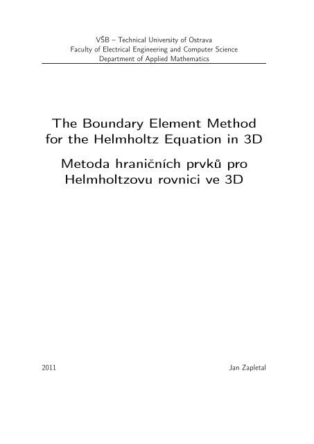
4 1 Function Spacesthe space C k (Ω) is a Banach space. Furthermore, we define C ∞ (Ω) as the space offunctions in C ∞ (Ω) that are continuously extendable to ∂Ω. Note that functions in thisspace do not have to be bounded nor uniformly continuous.For u ∈ C k (Ω) with k ∈ N 0 , a multiindex α, |α| ≤ k and λ ∈ (0, 1] we denote|D α u(x) − D α u(y)|H α,λ (u) := supx,y∈Ω ∥x − y∥ λ .x≠yWe define the space of Hölder continuous functions asC k,λ (Ω) := u ∈ C k (Ω): H α,λ (u) < ∞ for all α, |α| = k .Together with the norm∥u∥ C k,λ (Ω) := x∈Ω|α|≤ksup |D α u(x)| + |α|=k|D α u(x) − D α u(y)|supx,y∈Ω ∥x − y∥ λx≠ythe space C k,λ (Ω) is a Banach space. Setting k = 0 and λ = 1 we get the space C 0,1 (Ω)of Lipschitz continuous functions in Ω.Definition 1.1. A domain Ω ⊂ R d with a compact boundary ∂Ω is a C k,λ domain if thereexists a finite family of open sets {U i } n i=1 such that for every i ∈ {1, . . . , n} there exist• a Cartesian system of coordinates• ε i , δ i ∈ R + ,• a function a i : R d−1 → Rsatisfying(y i 1, . . . , y i d−1 , yi d ) = (yi , y i d ), where yi := (y i 1, . . . , y i d−1 ),• Γ i := U i ∩ ∂Ω = {(y i , y i d ): ∥yi ∥ < δ i , y i d = a i(y i )},• U + i:= {(y i , y i d ): ∥yi ∥ < δ i , a i (y i ) < y i d < a i(y i ) + ε i } ⊂ Ω,• U − i:= {(y i , y i d ): ∥yi ∥ < δ i , a i (y i ) − ε i < y i d < a i(y i )} ⊂ R d \ Ω,• a i ∈ C k,λ ({y i : ∥y i ∥ ≤ δ i }).For a Lipschitz domain, i.e., a C 0,1 domain (for an example of a Lipschitz domain inR 2 see Figure 1.1), the unit outward normal vector n = (n 1 , . . . , n d ) is defined almosteverywhere on ∂Ω. The coordinates n 1 , . . . , n d are bounded measurable functions on ∂Ω.Note that in this case the term ‘measurable’ corresponds to a surface measure defined on∂Ω. This abuse of terminology could be treated by introducing mappings from U i ∩ ∂Ω tothe global coordinate system and the measure could be understood as a (d−1) dimensionalLebesgue measure. However, throughout this text we use the simpler notation and referto this interpretation.

5∂Ωy i 2ΩU + iU − iΓ iy i 1Figure 1.1: Lipschitz domain in R 2 .1.2 Lebesgue and Sobolev SpacesFor a domain Ω ⊂ R d and p ∈ [1, ∞) we introduce L p (Ω) as the space of measurablefunctions u: Ω → C with1/p∥u∥ L p (Ω) := |u(x)| dx p < ∞.ΩRemark 1.2. In L p (Ω) we identify functions that are equal almost everywhere in Ω, thusthe elements of L p (Ω) are actually equivalence classes. By the relation u ∈ L p (Ω) weunderstand that there exists an equivalence class in L p (Ω) such that u belongs to it.For functions u ∈ L p (Ω) and v ∈ L q (Ω) with1p + 1 q= 1, p, q ∈ (1, ∞)it holds that uv ∈ L 1 (Ω) and the Hölder inequality|u(x)v(x)| dx ≤ ∥u∥ L p (Ω)∥v∥ L q (Ω)is satisfied.ΩThe L ∞ (Ω) space is defined as the space of measurable functions u: Ω → C satisfying∥u∥ L ∞ (Ω) := ess sup |u| :=Ωwhere µ d denotes the Lebesgue measure in R d .infE⊂Ωµ d (E)=0sup |u(x)| < ∞,x∈Ω\E

6 1 Function SpacesAll L p (Ω) spaces with p ∈ [1, ∞) ∪ {∞} are Banach spaces. Moreover, L 2 (Ω) is aHilbert space with the inner product⟨u, v⟩ L 2 (Ω) := u(x)v(x) dxinducing the norm ∥ · ∥ L 2 (Ω). In particular, for v = u, i.e., for the square of the L 2 (Ω)norm of u we get the equality∥u∥ 2 L 2 (Ω) = ⟨u, u⟩ L 2 (Ω) = u(x)u(x) dx = |u(x)| 2 dx.ΩFurthermore, we introduce L 1 loc(Ω) as the space of locally integrable measurable functionsu: Ω → C, i.e., for such functions it holds|u(x)| dx < ∞ for all compact subsets K ⊂ Ω.KNote that every function f ∈ L 1 loc(Ω) can be identified with a distribution defined as⟨f, ϕ⟩ := f(x)ϕ(x) dx for all ϕ ∈ C0 ∞ (Ω).ΩA partial derivative of a distribution F is a distribution D α F defined byΩ⟨D α F, ϕ⟩ := (−1) |α| ⟨F, D α ϕ⟩ for all ϕ ∈ C ∞ 0 (Ω). (1.1)ΩSince we deal with the Helmholtz equation in the following sections, it is necessary tointroduce Sobolev spaces of the first order. We define W 1,p (Ω) asW 1,p (Ω) :=u ∈ L p (Ω):∂u∈ L p (Ω) for k ∈ {1, . . . , d} ,∂x kwhere the derivatives must be considered in the distributional sense. Hence, W 1,p (Ω) is asubspace of L p (Ω). We denote by W 1,p0 (Ω) the closure of C0 ∞(Ω) in the space W 1,p (Ω).Both previously introduced spaces are Banach spaces for p ∈ [1, ∞) ∪ {∞} with respect tothe norm d1/p∥u∥ W 1,p (Ω) := |u(x)| p +∂up (x)Ω∂x k dx. (1.2)According to Theorem 3.22 in [1], for Lipschitz domains it holds that the set of functionsin C ∞ 0 (Rd ) restricted to Ω is dense in W 1,p (Ω) and thus for every function u ∈ W 1,p (Ω)there exists a sequence (ϕ n ) ⊂ C ∞ 0 (Rd ) such thatk=1lim ∥ϕ n | Ω − u∥ W 1,p (Ω) = 0.

7For a special choice of p = 2 we get Hilbert spaces H 1 (Ω) := W 1,2 (Ω) and H0 1 (Ω) :=W 1,20 (Ω) equipped with the inner product⟨u, v⟩ H 1 (Ω) := ⟨u, v⟩ L 2 (Ω) + ⟨∇u, ∇v⟩ L 2 (Ω)inducing the norm (1.2), which can be rewritten in the form∥u∥ H 1 (Ω) := ∥u∥ W 1,2 (Ω) = ∥u∥ 2 L 2 (Ω) + ∥∇u∥2 L 2 (Ω) .In the previous two formulae we used the notation⟨∇u, ∇v⟩ L 2 (Ω) :=∥∇u∥ 2 L 2 (Ω) :=dk=1dk=1ΩΩ∂u∂x k(x) ∂v∂x k(x) dx,∂u (x)∂x kIn the following text we also consider a more restricted space H 1 (Ω, ∆ + κ 2 ) ⊂ H 1 (Ω)with κ ∈ R + defined asH 1 (Ω, ∆ + κ 2 ) := {u ∈ H 1 (Ω): ∆u + κ 2 u ∈ L 2 (Ω)}, (1.3)where for smooth functions the symbol ∆ stands for the Laplace operator defined as∆u :=d ∂ 2 u.∂x 2 k=1 kNote that for a non-smooth function u the corresponding function ∆u + κ 2 u from thedefinition (1.3) must be interpreted in the distributional sense, i.e., using the definition ofdistributional derivatives (1.1), ∆u + κ 2 u is a distribution satisfying⟨∆u + κ 2 u, ϕ⟩ =d ∂ 2 u∂x 2 , ϕ + κ 2 ⟨u, ϕ⟩ =kk=12dk=1dx.= ⟨u, ∆ϕ + κ 2 ϕ⟩ for all ϕ ∈ C ∞ 0 (Ω). u, ∂2 ϕ∂x 2 + κ 2 ⟨u, ϕ⟩k(1.4)We say that ∆u + κ 2 u ∈ L 2 (Ω) in the distributional sense if there exists a functionv ∈ L 2 (Ω) satisfyingv(x)ϕ(x) dx = u(x) ∆ϕ(x) + κ 2 ϕ(x) dx for all ϕ ∈ C0 ∞ (Ω).ΩTogether with the normΩ∥u∥ H 1 (Ω,∆+κ 2 ) :=∥u∥ 2 H 1 (Ω) + ∥∆u + κ2 u∥ 2 L 2 (Ω)

8 1 Function Spacesthe space H 1 (Ω, ∆ + κ 2 ) is a Hilbert space.Finally, we introduce Hloc 1 (Ω) and H1 loc (Ω, ∆ + κ2 ) asu ∈ Hloc 1 (Ω) ⇔ u ∈ H1 ( Ω) for all open bounded subsets Ω ⊂ Ω,u ∈ Hloc 1 (Ω, ∆ + κ2 ) ⇔ u ∈ H 1 ( Ω, ∆ + κ 2 ) for all open bounded subsets Ω ⊂ Ω.Note that for a bounded domain Ω we haveHloc 1 (Ω) = H1 (Ω),Hloc 1 (Ω, ∆ + κ2 ) = H 1 (Ω, ∆ + κ 2 ).1.3 Lebesgue and Sobolev Spaces on ManifoldsSince the most important computations in the boundary element method take place onthe boundary, it is necessary to introduce appropriate function spaces defined on ∂Ω.For p ∈ [1, ∞) we denote by L p (∂Ω) the space of functions u : ∂Ω → C satisfying∥u∥ L p (∂Ω) :=∂Ω|u(x)| p ds 1/p< ∞.Furthermore, we introduce L ∞ (∂Ω) as the space of functions u: ∂Ω → C such that∥u∥ L ∞ (∂Ω) := ess sup |u| :=∂ΩinfE⊂∂Ωµ(E)=0sup |u(x)| < ∞.x∈∂Ω\ESimilarly as for the Lebesgue spaces defined on Ω, the elements of L p (∂Ω) are actuallyequivalence classes of functions (see Remark 1.2).Let us recall the trace theorem generalizing the concept of a restriction of a functionto the boundary (see Theorem 2.6.8 in [15]).Theorem 1.3 (On Traces). Let Ω ⊂ R d denote a Lipschitz domain. Then there exists aunique linear continuous mappingγ 0 : H 1 loc (Ω) → L2 (∂Ω)satisfyingu ∈ C ∞ (Ω): γ 0 u = u| ∂Ω .The function γ 0 u ∈ L 2 (∂Ω) is called the (Dirichlet) trace of the function u ∈ H 1 loc (Ω).Remark 1.4. The trace theorem allows an alternative definition of H0 1 (Ω) asH 1 0 (Ω) := {u ∈ H 1 (Ω): γ 0 u = 0}.

9Note that the trace operator is not surjective, i.e., there exist functions in L 2 (∂Ω) thatare not traces of any function in Hloc 1 (Ω). Therefore, we introduce H1/2 (∂Ω) as the tracespace of Hloc 1 (Ω), i.e.,H 1/2 (∂Ω) := γ 0 (Hloc 1 (Ω)).Obviously, H 1/2 (∂Ω) is a linear subset of L 2 (∂Ω). Equipped with the Sobolev–Slobodeckiinorm ∥u∥ H 1/2 (∂Ω) := ∥u∥ 2 L 2 (∂Ω) + |u(x) − u(y)| 2 1/2∥x − y∥ 3 ds x ds y∂Ωthe space is complete. Note that for a bounded domain Ω we have an equivalent norm∥u∥ H 1/2 (∂Ω) :=We define H −1/2 (∂Ω) as the dual space to H 1/2 (∂Ω), i.e., ∗H −1/2 (∂Ω) := H 1/2 (∂Ω)with the standard supremum norm∂Ωinf ∥v∥ H 1 (Ω). (1.5)v∈H 1 (Ω)γ 0 v=u∥f∥ H −1/2 (∂Ω) :=supu∈H 1/2 (∂Ω)u≠0|⟨f, u⟩|∥u∥ H 1/2 (∂Ω). (1.6)For a relatively open part of the boundary Γ ⊂ ∂Ω we define the spacesH 1/2 (Γ ) := v = ṽ| Γ : ṽ ∈ H 1/2 (∂Ω) ,H 1/2 (Γ ) := v = ṽ| Γ : ṽ ∈ H 1/2 (∂Ω), supp ṽ ⊂ Γ , ∗H −1/2 (Γ ) := H 1/2 (Γ ),∗H −1/2 (Γ ) := H 1/2 (Γ ).These spaces will be used for the purposes of mixed boundary value problems. For a moredetailed treatment on this topic see [12] or [18].1.4 Generalized Normal DerivativesLet us now assume that Ω denotes a bounded domain. Recall that for a function u ∈ H 1 (Ω)there exists a unique trace γ 0 u ∈ H 1/2 (∂Ω) generalizing the notion of a restriction tothe boundary. To generalize a normal derivative in the same way we would need higherwould have to be inH 1 (Ω). In the following section we will, however, show that it is possible to introducenormal derivatives for functions in H 1 (Ω, ∆ + κ 2 ).regularity of u. Namely, the distributional partial derivatives ∂u∂x k

10 1 Function SpacesFirst of all, we recall how normal derivatives are treated in the finite element method.To derive the weak formulation of a boundary value problem we will use the first Green’sidentity.Theorem 1.5 (First Green’s Identity). Let Ω ⊂ R d be a bounded C 1 domain and let ndenote the unit exterior normal vector to ∂Ω. Then for u ∈ C 2 (Ω), v ∈ C 1 (Ω) the firstGreen’s identityis satisfied.Ω∆u(x)v(x) dx =∂Ω∂u∂nΩ(x)v(x) ds − ∇u(x)∇v(x) dx (1.7)Remark 1.6. The normal derivatives in the preceding theorem should be understood as∂u(x) := lim ⟨∇u(x − hn(x)), n(x)⟩∂n h→0 +for x ∈ ∂Ω.Corollary 1.7 (Second Green’s Identity). Let Ω ⊂ R d be a bounded C 1 domain and let ndenote the unit exterior normal vector to ∂Ω. Then for u, v ∈ C 2 (Ω) the second Green’sidentityΩ∆u(x)v(x) dx −is satisfied.Ωu(x)∆v(x) dx =Consider the boundary value problem∂Ω∂u∂n∂Ω(x)v(x) ds − u(x) ∂v (x) ds (1.8)∂n⎧−(∆u + κ⎪⎨2 u) = 0 in Ω,u = g D on Γ D ,(1.9)⎪⎩ ∂u∂n = g N on Γ Nwith a bounded C 1 domain Ω, non-overlapping sets Γ D , Γ N ⊂ ∂Ω such that Γ D ∪ Γ N = ∂Ωand g D , g N ∈ C(∂Ω). Considering a classical solution u ∈ C 2 (Ω), we can multiply theequation by a test function v ∈ V := {v ∈ C 2 (Ω): v| ∂Ω = 0 on Γ D } to obtain− ∆u(x)v(x) dx − κ 2 u(x)v(x) dx = 0 for all v ∈ V.ΩΩApplying the first Greens’s identity (1.7) we obtain∇u(x)∇v(x) dx − κ 2 u(x)v(x) dx = g N (x)v(x) ds for all v ∈ V.ΩΩΓ NThis formulation, however, is also valid for more general settings given in the followingdefinition.

11Definition 1.8 (Weak Solution). Consider the boundary value problem (1.9) with abounded Lipschitz domain Ω, non-overlapping measurable sets Γ D , Γ N ⊂ ∂Ω such thatΓ D ∪ Γ N = ∂Ω, g D ∈ H 1/2 (Γ D ) and g N ∈ L 2 (Γ N ). Then u ∈ H 1 (Ω) is a weak solution to(1.9) if it satisfies⎧ ⎪⎨ ∇u(x)∇v(x) dx − κ 2 u(x)v(x) dx = g N (x)γ 0 v(x) ds for all v ∈ V,ΩΩΓ N⎪⎩γ 0 u = g D on Γ DwithV := {v ∈ H 1 (Ω): γ 0 v = 0 on Γ D }The advantage of the weak formulation is that the Neumann boundary condition istransformed into the term Γ Ng N (x)γ 0 v(x) dsand thus the normal derivatives of the solution do not appear in the weak formulation.However, for the purposes of the boundary element method the concept of normalderivatives has to be generalized. Using the definition of distributional partial derivatives(1.1) we get for u ∈ L 1 loc (Ω)d ∂ 2 ud ∂u⟨∆u, ϕ⟩ =∂x 2 , ϕ = − , ∂ϕ =k=1 k∂x k ∂x kk=1= u(x)∆ϕ(x) dx for all ϕ ∈ C0 ∞ (Ω).dk=1For u ∈ H 1 (Ω, ∆ + κ 2 ) we may use the middle term from (1.10)⟨∆u, ϕ⟩ = −dk=1 ∂u, ∂ϕ = −∂x k ∂x kand rewrite (1.10) as∆u(x)ϕ(x) dx = −ΩΩdk=1Ω∂u(x) ∂ϕ (x) dx∂x k ∂x k u, ∂2 ϕ∂x 2 = ⟨u, ∆ϕ⟩kfor all ϕ ∈ C ∞ 0 (Ω)(1.10)∇u(x)∇ϕ(x) dx for all ϕ ∈ C ∞ 0 (Ω). (1.11)Let u ∈ H 1 (Ω, ∆ + κ 2 ) be an arbitrary but fixed function. We define a functional˜L u : H 1 (Ω) → C as˜L u (v) := ∇u(x)∇v(x) dx + ∆u(x) + κ 2 u(x) v(x) dx − κ 2 u(x)v(x) dxΩΩΩApparently, ˜L u is linear and due to the Hölder inequality we have|˜L u (v)| ≤ ∥∇u∥ L 2 (Ω)∥∇v∥ L 2 (Ω) + ∥∆u + κ 2 u∥ L 2 (Ω)∥v∥ L 2 (Ω) + κ 2 ∥u∥ L 2 (Ω)∥v∥ L 2 (Ω)≤ (2 + κ 2 )∥u∥ H 1 (Ω,∆+κ 2 )∥v∥ H 1 (Ω),

13In the previous paragraphs we showed how to generalize the concept of a normal derivativeof a function in H 1 (Ω, ∆ + κ 2 ) with a bounded domain Ω. However, it is also possibleto introduce the Neumann trace operator γ 1 for functions defined on an unbounded domain.Since the trace is only dependable on the behaviour of the function in the vicinityof the boundary, we haveγ 1 : H 1 loc (Ω, ∆ + κ2 ) → H −1/2 (∂Ω).Because H 1 loc (Ω, ∆+κ2 ) coincides with H 1 (Ω, ∆+κ 2 ) for bounded domains, the precedingdefinitions agree with this concept. For a more detailed treatment of this topis see [15],Section 2.7.Note that for a function u ∈ H 2 (Ω), whereH 2 (Ω) := u ∈ L 2 (Ω): D α u ∈ L 2 (Ω) for |α| ≤ 2 ,we have⟨γ 1 u, γ 0 v⟩ =dk=1∂Ωγ 0 ∂u(x)n k (x)γ 0 ∂uv(x) ds =∂x k ∂Ω ∂n (x)γ0 v(x) ds.

152 Helmholtz EquationLet us first recall the well-known wave equation∂ 2 U∂t 2 = c2 ∆U in (0, τ) × Ω (2.1)describing the wave propagation in a homogeneous, isotropic and friction-free medium witha constant speed of propagation c. For the derivation of the wave equation (2.1) see, e.g.,[10] or [9].In the case of time harmonic waves, i.e., waves of the formU(t, x) = Re u(x)e −iωtwith a complex-valued scalar function u: Ω → C, the imaginary unit i and ω ∈ R + denotingthe angular frequency, we can reduce the wave equation (2.1) as follows. For the solutionU we getU(t, x) = Re u(x)e −iωt = (Re u) cos ωt + (Im u) sin ωt. (2.2)Inserting (2.2) into (2.1) and dividing by c 2 we obtain− ω2c 2 (Re u) cos ωt + (Im u) sin ωt= (∆ Re u) cos ωt + (∆ Im u) sin ωt,which after rearranging yieldscos ωt∆ Re u + ω2c 2 Re u + sin ωt∆ Im u + ω2c 2 Im u = 0. (2.3)The equation (2.3) is satisfied in some time interval (0, τ) if it holdsi.e., if the equation∆ Re u + ω2ω2Re u = 0 ∧ ∆ Im u + Im u = 0,c2 c2 ∆u + ω2c 2 u = 0in Ωis satisfied. Defining the wave number κ asκ := ω c ∈ R +we finally obtain the Helmholtz equation∆u + κ 2 u = 0 in Ω.

17the boundary value problem (see, e.g., [6], [9])⎧∆u + κ 2 u = 0 in Ω ext ,⎪⎨⎪⎩x ∇u s (x),∥x∥u s + u i = u in Ω ext ,− iκu s (x)u = 0 on Γ D ,∂u∂n = 0 on Γ N, 1 = O ∥x∥ 2for ∥x∥ → ∞(2.4)with u := u s + u i denoting the total wave. The homogeneous Dirichlet and Neumannboundary conditions represent the so-called sound-soft and sound-hard scattering, respectively.Assuming that the source of the incident wave is remote enough, we can approximateu i by plane waves, i.e.,u i (x) := e iκ⟨x,d⟩with d denoting the normalized propagation direction. Because such u i satisfies the Helmhholtzequation, we can reduce the problem (2.4) to⎧⎪⎨⎪⎩ ∇u s (x),x∥x∥∆u s + κ 2 u s = 0 in Ω ext ,u s = −u i on Γ D ,∂u s∂n = −iκ⟨d, n⟩u i on Γ N , − iκu s (x)1 = O ∥x∥ 2 for ∥x∥ → ∞with n denoting the unit outward normal vector to ∂Ω. The total wave is then given bythe formula u = u s + u i .2.2 Fundamental SolutionThe knowledge of the fundamental solution is essential for the derivation of the representationformulae and the corresponding boundary integral equations. The fundamentalsolution for the Helmholtz equation in R 3 is introduced by the following definition.Definition 2.1 (Fundamental Solution). The function v : R 3 × R 3 → C defined asv κ (x, y) := 1 e iκ∥x−y∥4π ∥x − y∥is called the fundamental solution for the Helmholtz equation in R 3 .In the following theorems we provide some properties of the fundamental solution v κ ,which will be used for the derivation of the representation formulae.

20 2 Helmholtz Equation∂ΩΩ εεynB ε∂B εFigure 2.2: Illustration for the proof of Theorem 2.5.with⎡⎢det J(r, ϑ, ψ) = det ⎣∂x 1∂r∂x 2∂r∂x 3∂r∂x 1∂ϑ∂x 2∂ϑ∂x 3∂ϑ∂x 1∂ψ∂x 2∂ψ∂x 3∂ψ⎤⎥⎦ = r 2 cos ψ.According to Theorem 2.4 we have ṽ κ ∈ L 1 loc (R3 ) and we can identify ṽ κ with a distributionṽ κ : C0 ∞(R3 ) → C defined as⟨ṽ κ , ϕ⟩ :=ṽ κ (x)ϕ(x) dx =R 3 v κ (x, y)ϕ(x) dx.R 3Theorem 2.5. Let y ∈ R 3 . Then the function ṽ κ : R 3 → C,satisfiesṽ κ (x) := v κ (x, y)∆ṽ κ + κ 2 ṽ κ = −δ yin the distributional sense, i.e.,∆ṽκ + κ 2 ṽ κ , ϕ = ⟨−δ y , ϕ⟩ := −ϕ(y) for all ϕ ∈ C ∞ 0 (R 3 ).Proof. Let y ∈ R 3 and ϕ ∈ C ∞ 0 (R3 ) be chosen arbitrarily. We have to prove that∆ṽκ + κ 2 ṽ κ , ϕ = −ϕ(y).Similarly as in (1.4), we get for the left-hand side∆ṽκ + κ 2 ṽ κ , ϕ = ⟨ṽ κ , ∆ϕ + κ 2 ϕ⟩.

21Because ṽ κ ∈ L 1 loc (R3 ) (see Theorem 2.4), we can rewrite the last term of the previousformula as⟨ṽ κ , ∆ϕ + κ 2 ϕ⟩ = v κ (x, y) ∆ϕ(x) + κ 2 ϕ(x) dx =: I.R 3Let us now choose a smooth enough bounded domain Ω ⊂ R 3 such that supp ϕ ⊂ Ω,y ∈ Ω. Furthermore, we denote B ε (y) := {x ∈ R 3 : ∥x − y∥ < ε} and Ω ε := Ω \ B ε (y)(see Figure 2.2). Since the domain Ω ε does not contain the point y, it holds∆ x v κ (x, y) + κ 2 v κ (x, y) = 0for all x ∈ Ω εand we obtainI = v κ (x, y) ∆ϕ(x) + κ 2 ϕ(x) dx = lim v κ (x, y) ∆ϕ(x) + κ 2 ϕ(x) dxR 3 ε→0 + Ω ε= lim v κ (x, y) ∆ϕ(x) + κ 2 ϕ(x) − ∆ x v κ (x, y) + κ 2 v κ (x, y) ϕ(x) dxε→0 + Ω ε =0= lim v κ (x, y)∆ϕ(x) − ∆ x v κ (x, y)ϕ(x) dx.ε→0 + Ω εUsing the second Green’s identity (1.8) and the fact that ϕ = ∂ϕ∂n= 0 on ∂Ω we haveI = lim∂ϕ∂n (x)v κ(x, y) dx − lim =:I 1ε→0 +∂B ε(y)∂v κ(x, y)ϕ(x) dx .∂n x =:I 2ε→0 +∂B ε(y)To evaluate the integrals I 1 and I 2 we parametrize the sphere ∂B ε (y) using (2.6) withr = ε. Because for x ∈ ∂B ε (y) we have ∥x − y∥ = ε, we obtainI 1 = 1 2π π24π 0 − π 2= 14π εeiκε 2π0e iκεε π2− π 2∂ϕ y + ε(cos ϑ cos ψ, sin ϑ cos ψ, sin ψ) ε 2 cos ψ dψ dϑ∂n∂ϕ y + ε(cos ϑ cos ψ, sin ϑ cos ψ, sin ψ) cos ψ dψ dϑ.∂nBecause ϕ ∈ C ∞ 0 (R3 ) andwe obtain for the first integrallim εe iκε = 0,ε→0 +limε→0 +I 1 = 0.To evaluate I 2 we first have to express the normal derivative ∂vκ∂n x∂B ε (y). For the gradient of v κ we get= ⟨∇ x v κ , n⟩ on∇ x v κ (x, y) = 1 iκ∥x − y∥ − 1eiκ∥x−y∥4π ∥x − y∥ 3 (x − y),

22 2 Helmholtz Equationthe normal vector n can be expressed as (see Figure 2.2)n(x) = − 1 (x − y)εand thusHence, we have∂v κ(x, y) = 1∂n x 4π1ε1 − iκ∥x − y∥eiκ∥x−y∥ .∥x − y∥I 2 = 1 2π π24π 0 − π 21ε1 − iκεeiκε ϕ y + ε(cos ϑ cos ψ, sin ϑ cos ψ, sin ψ) ε 2 cos ψ dψ dϑε= 1 2π π2e iκε (1 − iκε)ϕ y + ε(cos ϑ cos ψ, sin ϑ cos ψ, sin ψ) cos ψ dψ dϑ.4π 0 − π 2The Lebesgue dominated convergence theorem allows us to interchange the limit and theintegration. Moreover, because ϕ ∈ C ∞ 0 (R3 ) andlim e iκε (1 − iκε) = 1,ε→0 +we obtainand finallylim I 2 = 1 2π π2ϕ(y) cos ψ dψ dϑ = ϕ(y)ε→0 + 4π 0 − π 2which was to be proved.I = ⟨∆ṽ κ + κ 2 ṽ κ , ϕ⟩ = limε→0 +I 1 − limε→0 +I 2 = −ϕ(y) = ⟨−δ y , ϕ⟩,2.3 Representation FormulaeThe following two theorems form the basis of the boundary element method, providingformulae for calculating the solution to a boundary value problem in any point of thegiven domain. Firstly, we focus on interior problems, i.e., problems on bounded domains.Theorem 2.6 (Representation Formula for Bounded Domains). Let Ω ⊂ R 3 be a boundedC 1 domain, let v κ denote the fundamental solution for the Helmholtz equation in R 3 andlet n denote the unit outward normal vector to ∂Ω. Then for u ∈ C 2 (Ω) we have therepresentation formula∂uu(x) =∂Ω ∂n (y)v κ(x, y) ds y − u(y) ∂v κ(x, y) ds y∂Ω ∂n y− ∆u(y) + κ 2 u(y) v κ (x, y) dy for x ∈ Ω.Ω

23In particular, if u satisfies the Helmholtz equationthenu(x) =∂Ω∆u + κ 2 u = 0 in Ω,∂u∂n (y)v κ(x, y) ds y − u(y) ∂v κ(x, y) ds y for x ∈ Ω. (2.7)∂Ω ∂n yProof. The proof is constructed in the same way as in the case of Theorem 2.5. Let x ∈ Ωbe an arbitrary fixed point. Let us choose ε > 0 such thatB ε (x) := {y ∈ R 3 : ∥x − y∥ < ε} ⊂ B ε (x) ⊂ Ωand let us denote Ω ε := Ω \ B ε (x) (similar situation as in Figure 2.2 with points x and yswapped). From Theorem 2.2 and the symmetry of v κ we have∆ y v κ (x, y) + κ 2 v κ (x, y) = 0 for all y ∈ Ω ε .Using the second Green’s identity with functions u and v κ on Ω ε we obtain=0∆u(y) + κ 2 u(y) v κ (x, y) dy − u(y) ∆ y v κ (x, y) + κ 2 v κ (x, y) dyΩ ε Ω ε∂u=∂Ω ∂n (y)v κ(x, y) ds y − u(y) ∂v κ(x, y) ds y(2.8)∂Ω ∂n y+−∂B ε(x)∂u∂n (y)v κ(x, y) ds y =:I 1Because for y ∈ ∂B ε (x) we have ∥x − y∥ = ε andit holds thatn(y) = 1 (x − y),εu(y) ∂v κ(x, y) ds y∂B ε(x) ∂n y =:I 2.v κ (x, y) = 1 e iκε4π ε ,∇ y v κ (x, y) = 1 1 − iκεeiκε4π ε 3 (x − y),∂v κ(x, y) = ⟨∇ y v κ (x, y), n(y)⟩ = 1 1∂n y 4π ε 2 eiκε (1 − iκε)for all y ∈ ∂B ε (x). Using the parametrization as in the proof of Theorem 2.4 (but with xand y swapped) we have for the integral I 1I 1 = 14π 2π0 π2− π 2= 14π εeiκε 2π0e iκεε π2− π 2∂u x + ε(cos ϑ cos ψ, sin ϑ cos ψ, sin ψ) ε 2 cos ψ dψ dϑ∂n∂u x + ε(cos ϑ cos ψ, sin ϑ cos ψ, sin ψ) cos ψ dψ dϑ∂n

24 2 Helmholtz Equationand due to properties of uFor the integral I 2 we obtainlim I 1 = 0.ε→0 +I 2 = 1 2π π24π 0 − π 21ε 2 eiκε (1 − iκε)u x + ε(cos ϑ cos ψ, sin ϑ cos ψ, sin ψ) ε 2 cos ψ dψ dϑ= 1 2π π2e iκε (1 − iκε)u x + ε(cos ϑ cos ψ, sin ϑ cos ψ, sin ψ) cos ψ dψ dϑ4π 0 − π 2and using the Lebesgue dominated convergence theorem and qualities of u we haveFinally, letting ε → 0 + we obtain from (2.8)∆u(y) + κ 2 u(y) v κ (x, y) dylim I 2 = u(x).ε→0 +Ω=∂Ω∂u∂n (y)v κ(x, y) ds y − u(y) ∂v κ(x, y) ds y − u(x).∂Ω ∂n ySince the point x ∈ Ω was arbitrary, we have proved Theorem 2.6.When solving a problem of sound scattering or wave propagation described by theHelmholtz equation we are usually interested in the solution in an unbounded domain.The following theorem gives us the representation formula for such domains (see [6]).Theorem 2.7 (Representation Formula for Unbounded Domains). Let Ω ⊂ R 3 be abounded C 1 domain, let v κ denote the fundamental solution for the Helmholtz equation inR 3 and let n denote the unit outward normal vector to ∂Ω. Let us define Ω ext := R 3 \ Ω.Then for u ∈ C 2 (Ω ext ) satisfying∆u + κ 2 u = 0in Ω extand the Sommerfeld radiation condition x ∇u(x), − iκu(x)1∥x∥ = O ∥x∥ 2for ∥x∥ → ∞we have the representation formulau(x) = u(y) ∂v κ(x, y) ds y −∂n y∂Ω∂Ω∂u∂n (y)v κ(x, y) ds y for x ∈ Ω ext .

25Ωn to ∂Ω ε0n to ∂Ω∂Ω∂B ε (o)n to ∂Ω εΩ εFigure 2.3: Illustration for the proof of Theorem 2.7.Proof. Let B ε (0) := {y ∈ R 3 : ∥y∥ < ε}, where ε is taken such that Ω ⊂ B ε (0). Furthermore,let Ω ε := B ε (0) \ Ω (see Figure 2.3). We start with showing that|u(y)| 2 ds = O(1) for ε → ∞.∂B ε(0)From the radiation condition we deduce lim∂u2ε→∞ ∂n (y) − iκu(y) ds = 0. (2.9)∂B ε(0)BecauseIm u ∂ū = Re u Im ∂ū∂ū∂u∂u+ Im u Re = − Re u Im + Im u Re∂n∂n ∂n ∂n ∂n ,we get for the integrand from (2.9) ∂u 2∂n − iκu =∂uRe ∂n∂u2 + i Im∂n − iκ Re u + κ Im u = Re ∂u∂n+ κ 2 (Im u) 2 + 2κ Im u Re ∂u ∂n + Im ∂u∂n− 2κ Im ∂u ∂n Re u = ∂u∂n2+ κ 2 |u| 2 + 2κ Im 2 2+ κ 2 (Re u) 2u ∂ū ∂n

26 2 Helmholtz Equationand thus lim∂u 2ε→∞ ∂B ε(0) ∂n (y)Since+ κ 2 |u(y)| 2 ds + 2κ Im u(y) ∂ū∂B ε(0) ∂n (y) ds = 0. (2.10)Now we apply the first Green’s identity (1.7) in Ω ε for functions u and ū to obtain∂ū∆ū(y)u(y) dy + ∇ū(y)∇u(y) dy = (y)u(y) ds. (2.11)Ω ε Ω ε∂n∆ū + κ 2 ū = 0in Ω εand ∂Ω ε = ∂Ω ∪ ∂B ε (0), we can rewrite the formula (2.11) as|∇u(y)| 2 dy − κ 2 |u(y)| 2 ∂ūdy =Ω ε Ω ε ∂B ε(0) ∂n∂Ω(y)u(y) ds − ∂ū(y)u(y) ds, (2.12)∂nwhere we had to take into account the opposite direction of n for y ∈ ∂Ω (see Figure 2.3).Because the left-hand side of (2.12) is real, we obtain∂ūIm∂n∂Ω(y)u(y) ds = Im ∂ū(y)u(y) ds < ∞. (2.13)∂n∂B ε(0)Inserting (2.13) into (2.10) we getand thus lim∂u 2ε→∞ ∂B ε(0) ∂n (y)limε→∞∂B ε(0) ∂u 2∂n (y)∂Ω ε+ κ 2 |u(y)| 2 ds + 2κ Im u(y) ∂ū∂Ω ∂n (y) ds = 0+ κ 2 |u(y)| 2 ds = −2κ Im∂Ωu(y) ∂ū (y) ds < ∞.∂nBecause both terms on the left-hand side are non-negative, they have to be bounded forε → ∞. Therefore, we have proved that|u(y)| 2 ds = O(1) for ε → ∞. (2.14)∂B ε(0)From Theorem 2.3 we know that the radiation condition and thus also (2.14) is validfor the fundamental solution v κ . Using the Hölder inequality we thus obtain ∂vκI 1 := u(y) (x, y) − iκv κ (x, y) ds y∂B ε(0) ∂n y 1/2 ≤ |u(y)| 2 ds y ∂v κ2 1/2 (x, y) − iκv κ (x, y)∂B ε(0)∂B ε(0) ∂n y ds y → 0 for ε → ∞(2.15)

27andI 2 :=∂B ε(0) ∂uv κ (x, y)∂n (y) − iκu(y) ds y 1/2 ≤ |v κ (x, y)| 2 ds y ∂u2 1/2∂B ε(0)∂B ε(0) ∂n (y) − iκu(y) ds y → 0 for ε → ∞.(2.16)Finally, for the bounded domain Ω ε we can apply the representation formula (2.7) toobtain∂uu(x) =∂Ω ε∂n (y)v κ(x, y) ds y − u(y) ∂v κ(x, y) ds y∂Ω ε∂n y∂u= −∂n (y)v κ(x, y) ds y + u(y) ∂v κ(x, y) ds y + I 2 − I 1∂n y∂Ωfor all x ∈ Ω ε . Letting ε → ∞, using (2.15) and (2.16), we eventually getu(x) = u(y) ∂v κ∂u(x, y) ds y −∂n y ∂n (y)v κ(x, y) ds y∂Ωfor all x ∈ Ω ext , which was to be proved.Theorems 2.6 and 2.7 provide representation of the solution to the Helmholtz equationby means of boundary integrals. The functions( V ∂v κκ s)(x) := v κ (x, y)s(y) ds y and (W κ t)(x) := (x, y)t(y) ds y∂n y∂Ωare called potentials with density functions s, t. Although we have only discussed the caseof smooth data, in the following section we will show that the potentials can also be definedfor more general density functions and domains. The properties of the integral operatorsV κ and W κ will play a crucial role in obtaining the missing Cauchy data.∂Ω∂Ω∂Ω

293 Boundary Integral EquationsAt the beginning of this section we introduce some operator properties, which will be usedto prove existence and uniqueness of solutions to boundary integral equations derived laterin Section 3.5. In the following definitions we assume X and Y to be some Hilbert spaces.Definition 3.1. A linear operator A: X → X ∗ is X-elliptic if there exists a constantc A 1 ∈ R + such that the inequalityholds for all u ∈ X.Re ⟨Au, u⟩ ≥ c A 1 ∥u∥ 2 XDefinition 3.2. A linear operator A: X → Y is bounded if there exists a constant c A 2 ∈ R +such that the inequality∥Au∥ Y ≤ c A 2 ∥u∥ Xholds for all u ∈ X.Remark 3.3. Note that for linear operators boundedness is equivalent to continuity.Definition 3.4. A linear operator A: X → X ∗ is coercive if there exists a compactoperator C : X → X ∗ and a constant c A 1 ∈ R + such that the Gårdings inequalityholds for all u ∈ X.∂ΩRe ⟨(A + C)u, u⟩ ≥ c A 1 ∥u∥ 2 XIn the previous section we showed that in the smooth case the solution to the Helmholtzequation on a bounded domain can be represented as∂uu(x) =∂n (y)v κ(x, y) ds y − u(y) ∂v κ(x, y) ds y for x ∈ Ω. (3.1)∂n yFor the solution on an unbounded domain we have similarly∂uu(x) = −∂n (y)v κ(x, y) ds y + u(y) ∂v κ(x, y) ds y for x ∈ Ω ext . (3.2)∂n y∂Ω∂ΩIn both cases the solution u is determined by the Cauchy data, i.e., by the values of thesolution on the boundary and its normal derivatives. However, these data are not givenbeforehand as the boundary value problem would be overdetermined. When considering amixed problem, we are only given Dirichlet data on a part of the boundary and Neumanndata on the remaining part. In this section we show how the Cauchy couple can be obtainedfrom boundary integral equations derived from the representation formulae (3.1) and (3.2).Afterwards, these formulae can be used to compute the solution in any point x ∈ Ω orx ∈ Ω ext , respectively.∂Ω

30 3 Boundary Integral EquationsIntroducing the integral operatorsV κ : H −1/2 (∂Ω) → Hloc 1 (Ω), ( V κ s)(x) :=W κ : H 1/2 (∂Ω) → Hloc 1 (Ω), (W κt)(x) :=∂Ω∂Ωv κ (x, y)s(y) ds y , (3.3)∂v κ∂n y(x, y)t(y) ds y (3.4)with density functions s, t: ∂Ω → R allows us to rewrite the representation formulae (3.1)and (3.2) asu = V κ γ 1,int u − W κ γ 0,int u in Ω,u = − V κ γ 1,ext u + W κ γ 0,ext u in Ω ext .Remark 3.5. The operators V κ and W κ are usually called the single layer potential operatorand the double layer potential operator, respectively. However, there is a naming conflict.In the following sections we also use these terms for composite operators γ 0 Vκ and γ 0 W κ ,where γ 0 denotes the interior or exterior Dirichlet trace operator.Theorem 3.6. The operator V κ : H −1/2 (∂Ω) → Hloc 1 (Ω) is linear and continuous. Hence,for bounded domains there exists a constant c ∈ R + such that∥ V κ s∥ H 1 (Ω) ≤ c∥s∥ H −1/2 (∂Ω)for all s ∈ H −1/2 (∂Ω).Moreover, for all s ∈ H −1/2 (∂Ω) the function V κ s satisfies the Helmholtz equation in theweak sense (including the Sommerfeld radiation condition in the case of an unboundeddomain).Theorem 3.7. The operator W κ : H 1/2 (∂Ω) → Hloc 1 (Ω) is linear and continuous. Hence,for bounded domains there exists a constant c ∈ R + such that∥W κ t∥ H 1 (Ω) ≤ c∥t∥ H 1/2 (∂Ω)for all t ∈ H 1/2 (∂Ω).Moreover, for all t ∈ H 1/2 (∂Ω) the function W κ t satisfies the Helmholtz equation in theweak sense (including the Sommerfeld radiation condition in the case of an unboundeddomain).The preceding theorems allow us to seek the solution to the Helmholtz equation in theform u = V κ s or u = W κ t with unknown density functions s, t. This approach gives rise toindirect boundary element methods, which will be mentioned later.Properties of the above given potential operators, which will be discussed in the followingsections, can be found in [12] (see also [9] and [18]). These properties will be crucialfor the derivation of boundary integral equations (both direct and indirect), which will beused for the computation of the missing Cauchy data.

313.1 Single Layer Potential OperatorLet us first consider the operator V κ defined by (3.3). Recall, that for the Dirichlet traceoperator γ 0 we haveγ 0 : H 1 loc (Ω) → H1/2 (∂Ω).Combining this operator with V κ we obtain the single layer potential operatorV κ : H −1/2 (∂Ω) → H 1/2 (∂Ω), V κ := γ 0 Vκ .From linearity and continuity of γ 0 and V κ we get that the single layer potential operatoris linear and continuous, i.e., there exists a constant c ∈ R + such that∥V κ s∥ H 1/2 (∂Ω) ≤ c∥s∥ H −1/2 (∂Ω)for all s ∈ H −1/2 (∂Ω).Theorem 3.8. The single layer potential operator V κ : H −1/2 (∂Ω) → H 1/2 (∂Ω) is coercive.Proof. From Theorem 6.22 in [18] we have that he operator V 0 corresponding to the Laplaceequation, i.e., the Helmholtz equation with κ = 0, is H −1/2 (∂Ω)-elliptic. Moreover, theoperator C := V 0 − V κ : H −1/2 (∂Ω) → H 1/2 (∂Ω) is compact (see [18], Section 6.9). Thus,we have⟨(V κ + C)s, s⟩ = ⟨V 0 s, s⟩ ≥ c∥s∥ 2 H −1/2 (∂Ω)for all s ∈ H −1/2 (∂Ω),which completes the proof.Theorem 3.9. For s ∈ L ∞ (∂Ω) there holds the representation(V κ s)(x) = v κ (x, y)s(y) ds y for x ∈ ∂Ω.Proof. The proof is similar to the proof of Lemma 6.7 in [18].∂ΩMoreover, for the jump of the Dirichlet trace of the single layer potential V κ s on theboundary we have[γ 0 Vκ s] := γ 0,ext Vκ s − γ 0,int Vκ s = 0 for all s ∈ H −1/2 (∂Ω). (3.5)3.2 Adjoint Double Layer Potential OperatorIn Section 1.4 we introduced the Neumann trace operatorγ 1 : H 1 loc (Ω, ∆ + κ2 ) → H −1/2 (∂Ω).

32 3 Boundary Integral EquationsBecause the function V κ s satisfies the Helmholtz equation in the weak sense, we actuallyhaveV κ : H −1/2 (∂Ω) → H 1 loc (Ω, ∆ + κ2 )and thus we can compose the Neumann trace operator with the single layer potentialoperator to obtain the linear continuous mappingγ 1 Vκ : H −1/2 (∂Ω) → H −1/2 (∂Ω).Theorem 3.10. For s ∈ H −1/2 (∂Ω) there holdsγ 1,int ( V κ s)(x) = σ(x)s(x) + (K ∗ κs)(x) for x ∈ ∂Ω, (3.6)γ 1,ext ( V κ s)(x) = (σ(x) − 1)s(x) + (K ∗ κs)(x) for x ∈ ∂Ω, (3.7)where Kκ ∗ denotes the adjoint double layer potential operator(Kκs)(x) ∗ ∂v κ:= (x, y)s(y) ds y for x ∈ ∂Ω∂n xand∂Ω∂v κσ(x) := lim(x, y) ds y . (3.8)ε→0 +y∈Ω : ∥x−y∥=ε ∂n yProof. The proof can be found in [9], following Lemma 2.29.Remark 3.11. For the function σ we get1σ(x) = lim⟨x − y, n(y)⟩ eiκ∥x−y∥ 1ε→0 + 4π∥x − y∥ 2 ∥x − y∥ − iκ ds y .For n we can substituteto obtainy∈Ω : ∥x−y∥=ε1σ(x) = limε→0 + 4πn(y) =y∈Ω : ∥x−y∥=ε1 1= limε→0 + 4π eiκε ε 2 − iκ εx − y∥x − y∥e iκ∥x−y∥∥x − y∥ 1∥x − y∥ − iκ ds y1 ds y .y∈Ω : ∥x−y∥=εThus, the function σ depends on the interior angle of Ω in x ∈ ∂Ω. In particular, fordomains with boundary smooth in x ∈ ∂Ω we get σ(x) = 1/2. For Lipschitz domainsthe relation σ(x) = 1/2 is valid almost everywhere and we can simplify (3.6) and (3.7) toobtainγ 1,int ( V κ s)(x) = 1 2 s(x) + (K∗ κs)(x) for x ∈ ∂Ω, (3.9)γ 1,ext ( V κ s)(x) = − 1 2 s(x) + (K∗ κs)(x) for x ∈ ∂Ω. (3.10)

33For the jump of the Neumann trace of the single layer potential V κ s on the boundarywe thus get[γ 1 Vκ s] := γ 1,ext Vκ s − γ 1,int Vκ s = −s for all s ∈ H −1/2 (∂Ω).3.3 Double Layer Potential OperatorLet us now consider the operator W κ defined by (3.4). We define the corresponding boundaryintegral operator as the composition of γ 0 and W κ to get the mappingγ 0 W κ : H 1/2 (∂Ω) → H 1/2 (∂Ω).From the properties of the Dirichlet trace operator and the integral operator W κ we getthat γ 0 W κ is linear and continuous.Theorem 3.12. For t ∈ H 1/2 (∂Ω) there holdsγ 0,int (W κ t)(x) = (σ(x) − 1)t(x) + (K κ t)(x)γ 0,ext (W κ t)(x) = σ(x)t(x) + (K κ t)(x)for x ∈ ∂Ω,for x ∈ ∂Ω,where K κ denotes the double layer potential operator∂v κ(K κ t)(x) := (x, y)t(y) ds y∂n y∂Ωfor x ∈ ∂Ωand σ is defined by (3.8).Proof. The proof can be found in [9], following Lemma 2.32.Remark 3.13. Similarly as in Remark 3.11, for Lipschitz domains we get simplified formulaeγ 0,int (W κ t)(x) = − 1 2 t(x) + (K κt)(x) for x ∈ ∂Ω, (3.11)γ 0,ext (W κ t)(x) = 1 2 t(x) + (K κt)(x) for x ∈ ∂Ω. (3.12)For the jump of the Dirichlet trace of the double layer potential W κ t on the boundarywe have[γ 0 W κ t] := γ 0,ext W κ t − γ 0,int W κ t = t for all t ∈ H 1/2 (∂Ω).3.4 Hypersingular Integral OperatorFinally, we consider the hypersingular integral operator defined as the negative Neumanntrace of the double layer potential operator, i.e.,D κ : H 1/2 (∂Ω) → H −1/2 (∂Ω), D κ := −γ 1 W κ .

34 3 Boundary Integral EquationsAgain, the hypersingular operator is linear and there exists a constant c ∈ R + such that∥D κ t∥ H −1/2 (∂Ω) ≤ c∥t∥ H 1/2 (∂Ω)for all t ∈ H 1/2 (∂Ω).The hypersingular operator cannot be represented in the same way as the precedingoperators. For D κ t with a smooth enough density function t we have(D κ t)(x) = −γ 1 (W κ t)(x) = − limΩ∋˜x→x∈∂Ω ⟨n(x), ∇˜x(W κ t)(˜x)⟩.Recall, that for the double layer potential we have the representation∂v κ(W κ t)(˜x) = (˜x, y)t(y) ds y∂Ω ∂n y= 1 ⟨˜x − y, n(y)⟩e iκ∥˜x−y∥ 14π∥˜x − y∥ 3 − iκ∥˜x − y∥ 2 t(y) ds y .∂ΩInterchanging the limit with the computation of the normal derivative we obtainlim (W κt)(˜x)Ω∋˜x→x∈∂Ω= 14π lim⟨x − y, n(y)⟩eε→0 +y∈∂Ω iκ∥x−y∥ : ∥x−y∥≥εBy computing the normal derivative of the integrand we get1∥x − y∥ 3 −(D κ t)(x) = 14π lime⟨n(y),ε→0 +y∈∂Ω iκ∥x−y∥ n(x)⟩: ∥x−y∥≥ε+ ⟨x − y, n(y)⟩⟨x − y, n(x)⟩3∥x − y∥ 5 −iκ∥x − y∥ 2 t(y) ds y .iκ∥x − y∥ 2 − 1∥x − y∥ 33iκ∥x − y∥ 4 − κ 2 ∥x − y∥ 3 t(y) ds y . (3.13)Unfortunately, for ε → 0 + the integrand from (3.13) is not an integrable function. To expressD κ t explicitly we need some regularization procedure. For the Galerkin discretizationof the boundary integral equations we need to evaluate the bilinear form⟨D κ t, s⟩ ∂Ω := (D κ t)(x)s(x) ds x∂Ωinduced by the hypersingular operator. The following theorem gives us a representationusing surface curl operators.Theorem 3.14. For functions s, t ∈ H 1/2 (∂Ω) there holds the representation∂Ω(D κ t)(x)s(x) ds x = 1 4π− κ24π∂Ω∂Ω∂Ω∂Ωe iκ∥x−y∥∥x − y∥ ⟨curl ∂Ω t(y), curl ∂Ω s(x)⟩ ds y ds xe iκ∥x−y∥∥x − y∥ t(y)s(x)⟨n(x), n(y)⟩ ds y ds x

35with the surface curl operatorcurl ∂Ω t(y) := n(y) × ∇˜t(y)for y ∈ ∂Ω,where ˜t is some locally defined extension of t into the neighbourhood of ∂Ω.Proof. For the proof and more details see [13], Theorem 3.4.2 and [15], Theorem 3.3.22and Corrolary 3.3.24.Theorem 3.15. The hypersingular operator D κ : H 1/2 (∂Ω) → H −1/2 (∂Ω) is coercive.Proof. The proof is taken from [15], Lemma 3.9.8. The regularised hypersingular operatorD 0 + I corresponding to the Laplace equation is H 1/2 (∂Ω)-elliptic. Due to the compactembedding H 1/2 (∂Ω) ↩→↩→ H −1/2 (∂Ω) and the compactness of D κ − D 0 , the operatorC := I + D 0 − D κ : H 1/2 (∂Ω) → H −1/2 (∂Ω) is compact. Thus, we have⟨(D κ + C)t, t⟩ = ⟨(D 0 + I)t, t⟩ ≥ c∥t∥ 2 H 1/2 (∂Ω)for all t ∈ H 1/2 (∂Ω),which completes the proof.To conclude, for the jump of the Neumann trace of the double layer potential W κ t onthe boundary we have[γ 1 W κ t] := γ 1,ext W κ t − γ 1,int W κ t = 0 for all t ∈ H 1/2 (∂Ω). (3.14)3.5 Boundary Integral EquationsRecall that the solution to an interior boundary value problem for the Helmholtz equationcan be represented asu = −W κ γ 0,int u + V κ γ 1,int u in Ω.Applying the interior Dirichlet trace operator and using the definition of V κ and the property(3.11) we get the boundary integral equation 1γ 0,int u =2 I − K κ γ 0,int u + V κ γ 1,int u on ∂Ω (3.15)with the identity operator I. Similarly, applying the Neumann trace operator and using(3.9) and the definition of the hypersingular integral operator we obtain 1γ 1,int u = D κ γ 0,int u +2 I + K∗ κ γ 1,int u on ∂Ω. (3.16)The boundary integral equations (3.15), (3.16) can be rewritten as γ 0,int uγ 1,int = C int γ 0,int uu γ 1,int u

36 3 Boundary Integral Equationswith the Calderon projection matrix 1C int := 2 I − K κV κD κ12 I + K∗ κFor the solution in an unbounded domain we have the formula.u = W κ γ 0,ext u − V κ γ 1,ext u in Ω ext .Applying the Dirichlet and Neumann trace operators, respectively, and using properties(3.12), (3.10) and the definitions of the boundary integral operators V κ and D κ we get 1γ 0,ext u =2 I + K κ γ 0,ext u − V κ γ 1,ext u on ∂Ω ext , (3.17)γ 1,ext u = −D κ γ 0,ext u + 12 I − K∗ κγ 1,ext u on ∂Ω ext . (3.18)Again, the boundary integral equations (3.17), (3.18) can be rewritten as γ 0,ext uγ 1,ext = C ext γ 0,ext uu γ 1,ext uwith the Calderon projection matrix 1C ext := 2 I + K κ−V κ1−D κ 2 I − K∗ κTheorem 3.16. The Calderon operators C int and C ext are projection operators, i.e.,.(C int ) 2 = C int (C ext ) 2 = C ext .Proof. The proof is analogous to the proof of Lemma 6.18 in [18].Corollary 3.17. For the boundary integral operators we have the following identities 1 1V κ D κ = κ2 I + K 2 I − K κ ,D κ V κ = 12 I + K∗ κ 12 I − K∗ κD κ K κ = K ∗ κD κ ,K κ V κ = V κ K ∗ κ.Proof. The relations follow directly from the comparison of the matrices (C int ) 2 and C int .,

37The following theorems are standard results of functional analysis and will be usedto prove solvability of boundary integral equations studied in the next sections. In thetheorems we assume that X denotes a Hilbert space.Theorem 3.18 (Lax-Milgram Lemma). Let A: X → X ∗ denote a linear, bounded andX-elliptic operator. Then for any f ∈ X ∗ there exists a unique element u ∈ X satisfyingMoreover, there holds the estimatewith the ellipticity constant c A 1 .Au = f.∥u∥ X ≤ 1c A ∥f∥ X ∗1Proof. For the proof of the Lax-Milgram Lemma see [18], proof following Theorem 3.4 orany standard functional analysis textbook.Theorem 3.19 (Fredholm Alternative). Let K : X → X denote a compact operator. Eitherthe homogeneous equation(I − K)u = 0has a nontrivial solution u ∈ X or the inhomogeneous problem(I − K)u = fhas a unique solution u ∈ X for all f ∈ X. In the latter case there exists a constant c ∈ R +such that∥u∥ X ≤ c∥f∥ X for all f ∈ X.Proof. For the proof of the Fredholm Alternative see, e.g., [7], Theorem 2.2.9.Theorem 3.20. Let A: X → X ∗ denote a linear, bounded and coercive operator and letA be injective, i.e., from Au = 0 it follows u = 0. Then for every f ∈ X ∗ there exists aunique solution to the equationAu = f. (3.19)Moreover, there exists a constant c ∈ R + such that∥u∥ X ≤ c∥f∥ X ∗ for all f ∈ X ∗ . (3.20)Proof. From coercivity of A we know that there exists a compact operator C such that thelinear operator D := A + C : X → X ∗ is X-elliptic. From the Lax-Milgram Lemma 3.18we get that there exists the inverse operator D −1 : X ∗ → X. Therefore, we obtain thatthe equation (3.19) is equivalent toBu = D −1 f

38 3 Boundary Integral EquationswithB := D −1 A = D −1 (D − C) = I − D −1 C.From X-ellipticity of D and boundedness of A we get that B is bounded. Since we assumethat A is injective, it follows that the homogeneous equationD −1 Au = (I − D −1 C)u = 0only has the trivial solution and thus D −1 C is injective. The Fredholm Alternative 3.19with the compact operator K := D −1 C then guarantees a unique solution to (3.19) satisfyingthe estimate (3.20).Theorem 3.21. Let X denote a Hilbert space. Then it holds(∀x, y ∈ X, x ≠ y)(∃f ∈ X ∗ ): ⟨f, x⟩ ≠ ⟨f, y⟩.Proof. The theorem is a direct consequence of the well-known Hahn-Banach Theorem (see,e.g., [21], Theorem 1.B, Corollary 2 on pages 4–5).In Section 2.3 we introduced representation formulae for the solution to the Helmholtzequation with smooth enough data. The following theorems generalize the previous resultsfor a broader range of functions. For more details see [12], Theorems 6.10 and 7.12.Theorem 3.22. Let Ω be a bounded Lipschitz domain and let u ∈ H 1 (Ω, ∆ + κ 2 ) satisfythe Helmholtz equation in the weak sense. Then we have the representationu(x) = ( V κ γ 1,int u)(x) − (W κ γ 0,int u)(x) for x ∈ Ω. (3.21)Theorem 3.23. Let Ω be a bounded Lipschitz domain and let us denote Ω ext := R 3 \ Ω.Let u ∈ H 1 loc (Ωext , ∆ + κ 2 ) satisfy the Sommerfeld radiation condition and the Helmholtzequation in the weak sense. Then we have the representationu(x) = −( V κ γ 1,ext u)(x) + (W κ γ 0,ext u)(x) for x ∈ Ω ext . (3.22)Before we proceed to individual boundary value problems, we provide theorems regardingexistence and uniqueness of the weak solution to general boundary value problems forthe Helmholtz equation (see [12] and [15]).Theorem 3.24. The interior boundary value problem⎧⎪⎨∆u + κ 2 u = 0 in Ω,γ 0,int u = g D on Γ D ,⎪⎩γ 1,int u = g N on Γ Nwith a bounded Lipschitz domain Ω, non-overlapping sets Γ D , Γ N satisfying Γ D ∪ Γ N = ∂Ωand boundary conditions g D ∈ H 1/2 (Γ D ), g N ∈ H −1/2 (Γ N ) has a unique weak solution

39u ∈ H 1 (Ω, ∆+κ 2 ) if and only if κ 2 does not coincide with an eigenvalue λ of the eigenvalueproblem for the Laplace equation⎧⎪⎨−∆u λ = λu λ in Ω,γ 0,int u λ = 0 on Γ D ,(3.23)⎪⎩γ 1,int u λ = 0 on Γ N .Furthermore, if κ 2 coincides with an eigenvalue λ of (3.23), the solution exists if and onlyif⟨γ 0,int u λ , g N ⟩ ΓN = ⟨γ 1,int u λ , g D ⟩ ΓD for all corresponding eigenfunctions u λ .Theorem 3.25. Let us denote Ω ext := R 3 \ Ω with a bounded Lipschitz domain Ω. Theexterior boundary value problem⎧∆u + κ 2 u = 0 in Ω ext ,⎪⎨⎪⎩ ∇u(x),x∥x∥γ 0,ext u = g D on Γ D ,γ 1,ext u = g N on Γ N , − iκu(x)1 = O ∥x∥ 2for ∥x∥ → ∞with non-overlapping sets Γ D , Γ N satisfying Γ D ∪ Γ N = ∂Ω and boundary conditions g D ∈H 1/2 (Γ D ), g N ∈ H −1/2 (Γ N ) has a unique weak solution u ∈ H 1 loc (Ωext , ∆ + κ 2 ).3.5.1 Interior Dirichlet Boundary Value ProblemLet us first consider the interior Dirichlet boundary value problem for the Helmholtz equation∆u + κ 2 u = 0 in Ω,γ 0,int u = g Don ∂Ω(3.24)with a bounded Lipschitz domain Ω and the Dirichlet boundary condition g D ∈ H 1/2 (∂Ω).The solution to (3.24) is given by the representation formula (3.21) with γ 0,int u = g D , i.e.,u(x) = ( V κ γ 1,int u)(x) − (W κ g D )(x) for x ∈ Ω (3.25)with unknown Neumann trace data γ 1,int u ∈ H −1/2 (∂Ω). Applying the Dirichlet traceoperator γ 0,int to (3.25) we obtain the Fredholm integral equation of the first kind(V κ γ 1,int u)(x) = 1 2 g D(x) + (K κ g D )(x) for x ∈ ∂Ω. (3.26)Similarly, applying the Neumann trace operator γ 1,int to (3.25) we obtain the Fredholmintegral equation of the second kind12 γ1,int u(x) − (K ∗ κγ 1,int u)(x) = (D κ g D )(x) for x ∈ ∂Ω. (3.27)

40 3 Boundary Integral EquationsAccording to Theorem 3.21, the boundary integral equations (3.26) and (3.27) areequivalent to the variational problems 1⟨V κ γ 1,int u, s⟩ ∂Ω =2 I + K κ g D , s for all s ∈ H −1/2 (∂Ω)∂Ωand 12κI − K∗ γ 1,int u, t = ⟨D κ g D , t⟩ ∂Ω for all t ∈ H 1/2 (∂Ω),∂Ωrespectively, where⟨u, v⟩ ∂Ω :=∂Ωu(x)v(x) dsdenotes the duality pairing between H 1/2 (∂Ω) and H −1/2 (∂Ω).The equations (3.26) and (3.27) are not uniquely solvable for all κ ∈ R + . To show this,let us consider the Dirichlet eigenvalue problem for the Laplace equation−∆uλ = λu λ in Ω,γ 0,int (3.28)u λ = 0 on ∂Ω,which can be understood as the Helmholtz boundary value problem with κ 2 = λ and thehomogeneous Dirichlet boundary condition. Let λ ∈ R + be an eigenvalue of (3.28) and u λthe corresponding eigensolution. From the boundary integral equations (3.26) and (3.27)we get(V κ γ 1,int u λ )(x) = 1 2 γ0,int u λ (x) + (K κ γ 0,int u λ )(x) = 0 for x ∈ ∂Ω,12 γ1,int u λ (x) − (K ∗ κγ 1,int u λ )(x) = (D κ γ 0,int u λ )(x) = 0 for x ∈ ∂Ωand hence, if κ 2 coincides with the eigenvalue λ, the operators V κ and (1/2I − K ∗ κ) are notinjective and thus not invertible.On the other hand, for other values of κ both operators are injective. The coercivity ofthe single layer potential operator then ensures a unique solution to the boundary integralequation (3.26) (see Theorem 3.20). The following theorem describes the relation betweenthe weak solution and the solution given by the representation formula (see [12], Theorem7.5).Theorem 3.26. If u ∈ H 1 (Ω, ∆+κ 2 ) is a solution to the interior Dirichlet problem (3.24),then the Neumann trace γ 1,int u satisfies the boundary integral equation (3.26) and u hasthe representation (3.25).Conversely, if γ 1,int u satisfies the boundary integral equation (3.26), then the representationformula (3.25) defines a solution u ∈ H 1 (Ω, ∆+κ 2 ) to the interior Dirichlet problem(3.24).

41Another approach to computing the missing Neumann data is based on Theorems 3.6and 3.7 suggesting that we may seek the solution in the form of a single layer potentialor a double layer potentialu(x) = ( V κ s)(x) for x ∈ Ω (3.29)u(x) = −(W κ t)(x) for x ∈ Ω (3.30)with unknown density functions s, t. The density functions usually have no physical meaningand these methods are thus called indirect. The representations (3.29) and (3.30) giverise to the boundary integral equationsand the corresponding variational problemsV κ s(x) = γ 0,int u(x) for x ∈ ∂Ω, (3.31)12 t(x) − (K κt)(x) = γ 0,int u(x) for x ∈ ∂Ω⟨V κ s, t⟩ ∂Ω = ⟨γ 0,int u, t⟩ ∂Ω for all t ∈ H −1/2 (∂Ω), 1κ2 I − K t, s = ⟨γ 0,int u, s⟩ ∂Ω for all s ∈ H −1/2 (∂Ω).∂ΩNote that the structure of (3.31) and (3.26) is similar, only the right-hand sides are different.Thus, for values of κ 2 not coinciding with an eigenvalue of (3.28) we have a uniquesolution to (3.31).Although the indirect approach can also be used for other types of boundary valueproblems, in the following sections we only consider the direct boundary element methods.3.5.2 Interior Neumann Boundary Value ProblemSolution to the interior Neumann boundary value problem∆u + κ 2 u = 0 in Ω,γ 1,int u = g Non ∂Ω(3.32)with a bounded Lipschitz domain Ω and the Neumann trace g N ∈ H −1/2 (∂Ω) is given bythe representation formulau(x) = ( V κ g N )(x) − (W κ γ 0,int u)(x) for x ∈ Ω (3.33)with unknown Dirichlet trace data γ 0,int u. Applying the Dirichlet trace operator to (3.33)we obtain the Fredholm integral equation of the second kind12 γ0,int u(x) + (K κ γ 0,int u)(x) = (V κ g N )(x) for x ∈ ∂Ω. (3.34)

42 3 Boundary Integral EquationsSimilarly, applying the Neumann trace operator we get the Fredholm integral equation ofthe first kind(D κ γ 0,int u)(x) = 1 2 g N(x) − (K ∗ κg N )(x) for x ∈ ∂Ω. (3.35)Alternatively, we may consider the variational problems 1κ2 I + K γ 0,int u, s = ⟨V κ g N , s⟩ ∂Ω for all s ∈ H −1/2 (∂Ω),∂Ωand⟨D κ γ 0,int u, t⟩ ∂Ω = 12 I − K∗ κ g N , t∂Ωfor all t ∈ H 1/2 (∂Ω).corresponding to (3.34) and (3.35), respectively.To study the solvability of (3.34) and (3.35) let us first consider the Neumann eigenvalueproblem for the Laplace equation−∆uµ = µu µ in Ω,γ 1,int u µ = 0on ∂Ω.(3.36)Let µ ∈ R + be an eigenvalue of (3.36) with the corresponding eigensolution u µ . From(3.34) and (3.35) we obtain for κ 2 = µ12 γ0,int u µ (x) + (K κ γ 0,int u µ )(x) = (V κ γ 1,int u µ )(x) = 0 for x ∈ ∂Ω,(D κ γ 0,int u µ )(x) = 1 2 γ1,int u µ (x) − (K ∗ κγ 1,int u µ )(x) = 0 for x ∈ ∂Ω,implying that the function γ 0,int u µ belongs to the kernel of the boundary integral operatorsD κ and (1/2I + K κ ) and thus these operators are not invertible.For values of κ 2 not coinciding with eigenvalues of (3.36) both operators are injective.Since the hypersingular operator D κ is coercive, the boundary integral equation (3.35) isuniquely solvable.Theorem 3.27. If u ∈ H 1 (Ω, ∆ + κ 2 ) is a solution to the interior Neumann problem(3.32), then the Dirichlet trace γ 0,int u satisfies the boundary integral equation (3.35) and uhas the representation (3.33).Conversely, if γ 0,int u satisfies the boundary integral equation (3.35), then the representationformula (3.33) defines a solution u ∈ H 1 (Ω, ∆ + κ 2 ) to the interior Neumannproblem (3.32).

433.5.3 Interior Mixed Boundary Value ProblemIn many engineering problems we have to deal with mixed boundary conditions, i.e., withproblems of the type⎧⎪⎨∆u + κ 2 u = 0 in Ω,γ 0,int u = g D on Γ D ,(3.37)⎪⎩γ 1,int u = g N on Γ Nwith a bounded Lipschitz domain Ω, non-overlapping sets Γ D , Γ N such that Γ D ∪Γ N = ∂Ω,and functions g D ∈ H 1/2 (Γ D ) and g N ∈ H −1/2 (Γ N ). In the smooth case, the solution to(3.37) is given by the representation formulau(x) =γ 1,int u(y) v κ (x, y) ds y +Γ Dg N (y) v κ (x, y) ds yΓ N−Γ Dg D (y) ∂v κ∂n y(x, y) ds y −Γ Nγ 0,int u(y) ∂v κ∂n y(x, y) ds yfor x ∈ Ωwith unknown Dirichlet data γ 0,int u| ΓN and Neumann data γ 1,int u| ΓD . The missing Cauchydata can be obtained using any of the previously mentioned boundary integral equations(3.26), (3.27), (3.34) or (3.35). However, in this section we describe the so-called symmetricformulation using the single layer potential equation (3.26) and the hypersingular equation(3.35) simultaneously (see [17], Section 1.1.3).From Sections 3.5.1 and 3.5.2 we have the relations(V κ γ 1,int u)(x) = 1 2 γ0,int u(x) + (K κ γ 0,int u)(x) for x ∈ Γ D ⊂ ∂Ω,(D κ γ 0,int u)(x) = 1 2 γ1,int u(x) − (K ∗ κγ 1,int u)(x) for x ∈ Γ N ⊂ ∂Ω.(3.38)Let us define functionsH 1/2 (Γ N ) ∋ t := γ 0,int u − ˜g D ,H −1/2 (Γ D ) ∋ s := γ 1,int u − ˜g N(3.39)with some suitable extensions ˜g D , ˜g N defined on ∂Ω. Inserting the functions t, s into (3.38)we obtain the system of equations(V κ s)(x) − (K κ t)(x) = 1 2 ˜g D(x) + (K κ˜g D )(x) − (V κ˜g N )(x) for x ∈ Γ D ,(Kκs)(x) ∗ + (D κ t)(x) = 1 (3.40)2 ˜g N(x) − (Kκ˜g ∗ N )(x) − (D κ˜g D )(x) for x ∈ Γ Nequivalent to the variational formulationa(s, t, q, r) = F (q, r) for all q ∈ H −1/2 (Γ D ), r ∈ H 1/2 (Γ N ) (3.41)with unknown functions s ∈ H −1/2 (Γ D ), t ∈ H 1/2 (Γ N ), the bilinear forma(s, t, q, r) := ⟨V κ s, q⟩ ΓD − ⟨K κ t, q⟩ ΓD + ⟨K ∗ κs, r⟩ ΓN + ⟨D κ t, r⟩ ΓN

44 3 Boundary Integral Equationsand the right-hand side 1F (q, r) :=2 I + K κ ˜g D , q − ⟨V κ˜g N , q⟩ ΓD +Γ D 12κI − K∗ ˜g N , r − ⟨D κ˜g D , r⟩ ΓN .Γ NTheorem 3.28. If u ∈ H 1 (Ω, ∆ + κ 2 ) is a solution to the mixed problem (3.37), thenthe functions s, t satisfy the system of boundary integral equations (3.40) and u has therepresentationu(x) = ( V κ (s + ˜g N ))(x) − (W κ (t + ˜g D ))(x) for x ∈ Ω. (3.42)Conversely, if s, t satisfy the system of boundary integral equations (3.40), then therepresentation formula (3.42) defines a solution u ∈ H 1 (Ω, ∆ + κ 2 ) to the interior mixedproblem (3.37).3.5.4 Exterior Dirichlet Boundary Value ProblemLet us denote Ω ext := R 3 \ Ω with a simply connected bounded Lipschitz domain Ω ⊂ R 3so that ∂Ω ext = ∂Ω. Now we consider the exterior Dirichlet boundary value problem⎧∆u + κ 2 u = 0 in Ω ext ,⎪⎨γ 0,ext u = g D on ∂Ω,⎪⎩∇u(x) x∥x∥ − iκu(x)1 = O ∥x∥ 2for ∥x∥ → ∞(3.43)with the Dirichlet boundary condition g D ∈ H 1/2 (∂Ω). The solution can be representedasu(x) = −( V κ γ 1,ext u)(x) + (W κ g D )(x) for x ∈ Ω ext (3.44)with unknown Neumann trace data γ 1,ext u. Applying the Dirichlet trace operator to (3.44)we obtain the Fredholm integral equation of the first kind(V κ γ 1,ext u)(x) = − 1 2 g D(x) + (K κ g D )(x) for x ∈ ∂Ω. (3.45)Applying the Neumann trace gives rise to the Fredholm integral equation of the secondkind12 γ1,ext u(x) + (K ∗ κγ 1,ext u)(x) = −(D κ g D )(x) for x ∈ ∂Ω. (3.46)The boundary integral equations (3.45) and (3.46) are equivalent to the variationalproblems⟨V κ γ 1,ext u, s⟩ ∂Ω = − 1 2 I + K κ g D , s for all s ∈ H −1/2 (∂Ω) (3.47)∂Ωand 12κI + K∗ γ 1,ext u, t = ⟨−D κ g D , t⟩ ∂Ω for all t ∈ H 1/2 (∂Ω),∂Ω

45respectively.The unique solvability of the boundary integral equation (3.45) and the related variationalproblem (3.47) for κ 2 not coinciding with an eigenvalue of (3.28) follows from thediscussion in Section 3.5.1.Theorem 3.29. If u ∈ H 1 loc (Ωext , ∆ + κ 2 ) is a solution to the exterior Dirichlet problem(3.43), then the Neumann trace γ 1,ext u satisfies the boundary integral equation (3.45) andu has the representation (3.44).Conversely, if γ 1,ext u satisfies the boundary integral equation (3.45), then the representationformula (3.44) defines a solution u ∈ H 1 loc (Ωext , ∆ + κ 2 ) to the exterior Dirichletproblem (3.43).Note that Theorems 3.25 and 3.29 ensure that for all κ ∈ R + it holds− 1 2 I + K κ g D ∈ Im V κeven though the equation (3.45) is not uniquely solvable for some values of κ. To overcomethis difficulty, several approaches have been proposed. The approach of Brakhageand Werner (see [5]) suggests seeking the solution in the form of some complex linearcombination of a single and double layer potentials, i.e.,u(x) = (W κ w)(x) − iη( V κ w)(x)for x ∈ Ω extwith an unknown density function w ∈ L 2 (∂Ω). In [4], Burton and Miller suggest analternative to direct methods, using a complex linear combination of the boundary integralequations (3.17) and (3.18). To conclude, we also mention the CHIEF method proposedby Schenck (see [2]).3.5.5 Exterior Neumann Boundary Value ProblemNow we consider the exterior Neumann boundary value problem⎧∆u + κ 2 u = 0 in Ω ext ,⎪⎨γ 1,ext u = g N on ∂Ω, ⎪⎩x ∇u(x), − iκu(x)1∥x∥ = O ∥x∥ 2 for ∥x∥ → ∞(3.48)with an unbounded domain Ω ext := R 3 \ Ω and the Neumann trace g N ∈ H −1/2 (∂Ω). Thesolution is given byu(x) = −( V κ g N )(x) + (W κ γ 0,ext u)(x) for x ∈ Ω ext (3.49)with unknown Dirichlet trace data γ 0,ext u. Applying the Dirichlet trace operator to (3.49)we obtain the Fredholm integral equation of the second kind− 1 2 γ0,ext u(x) + (K κ γ 0,ext u)(x) = (V κ g N )(x) for x ∈ ∂Ω. (3.50)

46 3 Boundary Integral EquationsSimilarly, applying the Neumann trace operator we get the Fredholm integral equation ofthe first kind(D κ γ 0,ext u)(x) = − 1 2 g N(x) − (K ∗ κg N )(x) for x ∈ ∂Ω. (3.51)andInstead of equations (3.50) and (3.51) we may consider the variational problemsrespectively.− 1 2 I + K κ γ 0,ext u, s = ⟨V κ g N , s⟩ ∂Ω for all s ∈ H −1/2 (∂Ω),∂Ω⟨D κ γ 0,ext u, t⟩ ∂Ω =− 1 2 I − K∗ κ g N , t∂Ωfor all t ∈ H 1/2 (∂Ω), (3.52)The arguments for the unique solvability of the boundary integral equation (3.51) andthe corresponding variational problem (3.52) for κ 2 not coinciding with an eigenvalue of(3.36) are the same as in Section 3.5.2.Theorem 3.30. If u ∈ H 1 loc (Ωext , ∆ + κ 2 ) is a solution to the exterior Neumann problem(3.48), then the Dirichlet trace γ 0,ext u satisfies the boundary integral equation (3.51) andu has the representation (3.49).Conversely, if γ 0,ext u satisfies the boundary integral equation (3.51), then the representationformula (3.49) defines a solution u ∈ H 1 loc (Ωext , ∆ + κ 2 ) to the interior Neumannproblem (3.48).Note that Theorems 3.25 and 3.30 ensure that for all κ ∈ R + it holds− 1 2 I − K∗ κ g N ∈ Im D κand thus one of the methods mentioned at the end of the previous section can be used tocompute a solution to (3.51) with κ 2 coinciding with an eigenvalue of (3.36).3.5.6 Exterior Mixed Boundary Value ProblemFinally, let us consider the exterior mixed boundary value problem⎧⎪⎨⎪⎩ ∇u(x),x∥x∥∆u + κ 2 u = 0 in Ω ext ,γ 0,ext u = g D on Γ D ,γ 1,ext u = g N on Γ N , − iκu(x)1 = O ∥x∥ 2for ∥x∥ → ∞(3.53)

47with an unbounded domain Ω ext := R 3 \ Ω and boundary conditions g D ∈ H 1/2 (Γ D ),g N ∈ H −1/2 (Γ N ). In the smooth case the solution to (3.53) is given byu(x) = − γ 1,ext u(y) v κ (x, y) ds y − g N (y) v κ (x, y) ds yΓ D Γ N+ g D (y) ∂v κ(x, y) ds y + γ 0,ext u(y) ∂v κ(x, y) ds y for x ∈ Ω extΓ D∂n y Γ N∂n ywith unknown Cauchy data γ 0,ext u| ΓN and γ 1,ext u| ΓD . Similarly as for the interior mixedproblem we have the boundary integral equations(V κ γ 1,ext u)(x) = − 1 2 γ0,ext u(x) + (K κ γ 0,ext u)(x) for x ∈ Γ D ⊂ ∂Ω,(D κ γ 0,ext u)(x) = − 1 2 γ1,ext u(x) − (K ∗ κγ 1,ext u)(x) for x ∈ Γ N ⊂ ∂Ω.(3.54)Inserting the functions t, s defined by (3.39) into (3.54) yields(V κ s)(x) − (K κ t)(x) = − 1 2 ˜g D(x) + (K κ˜g D )(x) − (V κ˜g N )(x) for x ∈ Γ D ,(K ∗ κs)(x) + (D κ t)(x) = − 1 2 ˜g N(x) − (K ∗ κ˜g N )(x) − (D κ˜g D )(x) for x ∈ Γ N(3.55)and the equivalent variational formulationa(s, t, q, r) = F (q, r) for all q ∈ H −1/2 (Γ D ), r ∈ H 1/2 (Γ N ) (3.56)with unknown functions s ∈ H −1/2 (Γ D ), t ∈ H 1/2 (Γ N ), the bilinear forma(s, t, q, r) := ⟨V κ s, q⟩ ΓD − ⟨K κ t, q⟩ ΓD + ⟨K ∗ κs, r⟩ ΓN + ⟨D κ t, r⟩ ΓNand the right-hand sideF (q, r) := − 1 2 I + K κ ˜g D , q − ⟨V κ˜g N , q⟩ ΓD + − 1 Γ D2 I − K∗ κ ˜g N , r − ⟨D κ˜g D , r⟩ ΓN .Γ NTheorem 3.31. If u ∈ H 1 loc (Ωext , ∆ + κ 2 ) is a solution to the mixed problem (3.53), thenthe functions s, t satisfy the system of boundary integral equations (3.55) and u has therepresentationu(x) = −( V κ (s + ˜g N ))(x) + (W κ (t + ˜g D ))(x) for x ∈ Ω ext . (3.57)Conversely, if s, t satisfy the system of boundary integral equations (3.55), then therepresentation formula (3.57) defines a solution u ∈ H 1 loc (Ωext , ∆ + κ 2 ) to the interiormixed problem (3.53).

494 Discretization and Numerical RealizationIn this section we will describe the discretization of the boundary integral equations coveredin the previous part. We will discuss the collocation method as well as the more complicatedGalerkin scheme. The solution will be sought in approximating function spaces introducedbelow.We restrict ourselves to triangular meshes approximating the corresponding boundary∂Ω, i.e.,E∂Ω ≈and assume that neighbouring triangular elements either share a whole edge or a singlevertex. Each element τ k ⊂ R 3 with nodes x k 1, x k 2, x k 3can be described via theparametrizationR k (ξ) := x k 1+ R k ξ for ξ ∈ ˆτ, (4.1)where R k denotes the matrixk=1⎡τ kx k 21 − xk 11 x k 31 − xk 11R k := x k 2− x k 1x k 3− x k 1= ⎣x k 22 − xk 12 x k 32 − xk 1⎦ 2∈ R 3×2 (4.2)x k 23 − xk 13 x k 33 − xk 13and ˆτ ⊂ R 2 represents the reference triangle (see Figure 4.1a)ˆτ := {ξ ∈ R 2 : 0 < ξ 1 < 1, 0 < ξ 2 < 1 − ξ 1 }.Remark 4.1. Note that a function f defined on τ k can be identified with a function ˆfdefined on ˆτ and vice versa, i.e.,⎤f(x) = f(R k (ξ)) =: ˆf(ξ)for x ∈ τ k , ξ ∈ ˆτ.In the following text we use the symbol ∂Ω to denote the discretized boundary.4.1 Piecewise Constant Basis FunctionsFor every element τ k we define the function ψ k (see Figure 4.2a) as1 for x ∈ τ k ,ψ k (x) :=0 otherwise.Following Remark 4.1, the function ψ k can alternatively be defined via the reference function1 for ξ ∈ ˆτ,ˆψ(ξ) :=0 otherwise.

50 4 Discretization and Numerical Realizationξ 2x k 31x k 1τ kˆτ(a) Reference triangle.1ξ 1x 3x 2x k 2x 1(b) General triangle.Figure 4.1: Triangular mesh elements.ϕ k (x)ψ k (x)x kτ k(a) Piecewise constant basis function.(b) Piecewise affine basis function.Figure 4.2: Basis functions.Furthermore, we define the linear space T ψ (∂Ω) asT ψ (∂Ω) := span{ψ k } E k=1 ,where E denotes the number of elements. Obviously, dim T ψ (∂Ω) = E and every complexvaluedfunction g ψ ∈ T ψ (∂Ω) can be represented asg ψ =Eg k ψ kand thus it can be identified with a vector g := [g 1 , . . . , g E ] T ∈ C E .k=1A smooth enough function g can be approximated by a linear combination of piecewiseconstant functions in several ways. The simplest approach is to setg k = g(x k∗ )

51with x k∗denoting the midpoint of τ k . Alternatively, we can setg k = 1 3g(x k 1) + g(x k 2) + g(x k 3) .However, since we deal with functions in Lebesgue and Sobolev spaces, where we do notdistinguish between functions differing on a measure zero set, the above mentioned approximationsmay prove impossible. Hence, we introduce the projection P ψ : L 2 (∂Ω) → T ψ (∂Ω)minimizing the error∥g − P ψ g∥ L 2 (∂Ω),i.e.,P ψ g := arg min ∥g − g ψ∥ Lg ψ ∈T ψ (∂Ω) 2 (∂Ω).To find the coefficients g kf : R E → R as E f(g 1 , . . . , g E ) := g − 2g k ψ kk=1= ⟨g, g⟩ L 2 (∂Ω) − 2For the partial derivatives of f we getfor a real-valued function g we introduce the functionL 2 (∂Ω)=g −Eg k ψ k , g −k=1Eg k ⟨g, ψ k ⟩ L 2 (∂Ω) +k=1∂f∂g j= −2⟨g, ψ j ⟩ L 2 (∂Ω) + 2Moreover, for the Hessian of f we haveH f [j, i] =EEg k ψ kk=1Eg kk=1 l=1Eg k ⟨ψ k , ψ j ⟩ L 2 (∂Ω).k=1∂2 f∂g j ∂g i= 2⟨ψ i , ψ j ⟩,L 2 (∂Ω)g l ⟨ψ k , ψ l ⟩ L 2 (∂Ω).which is the double Gram matrix corresponding to the basis of T ψ (∂Ω). Hence, the Hessianis positive definite and to find the minimum of f we set ∂f∂g j= 0 to obtain the system oflinear equationsEg k ⟨ψ k , ψ j ⟩ L 2 (∂Ω) = ⟨g, ψ j ⟩ L 2 (∂Ω) for j ∈ {1, . . . , E}k=1with a unique solution g = [g 1 , . . . , g E ] T ∈ R E . Because∆ k for k = j,⟨ψ k , ψ j ⟩ L 2 (∂Ω) =0 otherwise,

52 4 Discretization and Numerical Realizationwhere ∆ k denotes the surface of τ k , we get for the piecewise constant approximationg k = 1 ∆ kτ kg(x) ds x .Let us now consider the case when g = Re g + i Im g is complex-valued. We thus searchfor coefficients g k = Re g k + i Im g k . For the L 2 error norm we get E g − 2g k ψ kk=1==∂Ω∂ΩL 2 (∂Ω) E = Re g + i Im g − 2(Re g k + i Im g k )ψ kk=1E Re g(x) − Re g k ψ k (x) + i Im g(x) −Re g(x) −k=1L 2 (∂Ω)E2Im g k ψ k (x) ds xk=12 ERe g k ψ k (x)+ Im g(x) −k=1 E = Re g − 2Re g k ψ kk=1L 2 (∂Ω) 2EIm g k (x)ψ k ds xk=1 E + Im g − 2Im g k ψ kk=1L 2 (∂Ω)and therefore, the problem is reduced to searching for appropriate coefficients of the tworeal-valued functions Re g and Im g as was described in the previous paragraph.The space T ψ (∂Ω) will be used for the approximation of the Neumann data, i.e., of thenormal derivatives on ∂Ω.4.2 Continuous Piecewise Affine Basis FunctionsLet N denote the number of all nodes of a given discretization. Then we define the familyof functions {ϕ k } N k=1continuous over the whole discretized boundary (see Figure 4.2b) as⎧⎪⎨ 1 for x = x k ,ϕ k (x) := 0 for x = x⎪⎩l ≠ x k ,piecewise affine otherwise.Furthermore, we define the linear space T ϕ (∂Ω) asT ϕ (∂Ω) := span{ϕ k } N k=1 .Obviously, dim T ϕ (∂Ω) = N. A restriction of a function ϕ k to an element τ l ⊂ supp ϕ kcan be identified with one of the functions ˆϕ 1 , ˆϕ 2 , ˆϕ 3 defined on the reference triangle asˆϕ 1 (ξ) := 1 − ξ 1 − ξ 2 , ˆϕ 2 (ξ) := ξ 1 , ˆϕ 3 (ξ) := ξ 2 for ξ ∈ ˆτ.

53k \ τ k x k 1x k 2x k 3local indices1 1 2 32 2 4 33 4 5 3....global indicesx 1 τ 1τ 2τ 3 x 5x 3 x 4x 2Figure 4.3: Connectivity table.We use the connectivity table (see Figure 4.3) to determine the mapping between globaland local indices of nodes building the triangular mesh. For example, the point x 4 is thesecond vertex of the triangle τ 2 , i.e., x 4 = x 2 2. Furthermore, for ϕ 4 | τ2 we haveϕ 4 | τ2 (x) = ϕ 4 | τ2 (R 4 (ξ)) = ˆϕ 2 (ξ) = ξ 1for x ∈ τ 2 , ξ ∈ ˆτ.As in the case of piecewise constant basis functions we can identify a functionT ϕ (∂Ω) ∋ g ϕ =Ng k ϕ kwith a vector [g 1 , . . . , g N ] T ∈ C N . For the approximation of a smooth enough function gwe can either use an interpolation, i.e.,k=1g k = g(x k ).For a function g ∈ L 2 (∂Ω) it is more appropriate to define the projection P ϕ : L 2 (∂Ω) →T ϕ (∂Ω) asP ϕ g := arg min ∥g − g ϕ∥ Lg 2 (∂Ω).ϕ∈T ϕ(∂Ω)The coefficients for real-valued functions can be found in the same way as for the piecewiseconstant functions as the solution to the system of linear equationsNg k ⟨ϕ k , ϕ j ⟩ L 2 (∂Ω) = ⟨g, ϕ j ⟩ L 2 (∂Ω)k=1for j ∈ {1, . . . , N}.In the case of complex-valued functions we can separately search for the real parts and theimaginary parts of the coefficients.The space T ϕ (∂Ω) will be used for the approximation of the Dirichlet data, i.e., thevalues of the solution on ∂Ω.4.3 Discretized Boundary Integral EquationsIn the following sections we describe the discretization of the boundary integral equationsderived in Section 3.5. Although the collocation method will be mentioned, we will prefer

54 4 Discretization and Numerical Realizationthe well studied Galerkin scheme based on the corresponding variational formulations. Toapproximate the Dirichlet and Neumann boundary data we use continuous piecewise affinefunctions and piecewise constant functions, respectively.4.3.1 Interior Dirichlet Boundary Value ProblemThe solution to the interior Dirichlet boundary value problem (3.24) is given by the representationformula (3.25) with unknown Neumann data g N := γ 1,int u. To compute themissing values we use the Fredholm integral equation of the first kind(V κ g N )(x) = 1 2 g D(x) + (K κ g D )(x) for x ∈ ∂Ωor equivalentlyg N (y)v κ (x, y) ds y = 1 2 g D(x) +∂Ωwith the fundamental solution v κ and the normal derivative∂Ωg D (y) ∂v κ∂n y(x, y) ds y for x ∈ ∂Ω (4.3)∂v κ(x, y) = 1 e iκ∥x−y∥(1 − iκ∥x − y∥)⟨x − y, n(y)⟩.∂n y 4π ∥x − y∥3 The corresponding variational formulation reads 1⟨V κ g N , s⟩ ∂Ω =2 I + K κ g D , sor∂Ω∂Ωfor all s ∈ H −1/2 (∂Ω)s(x) g N (y)v κ (x, y) ds y ds x∂Ω= 1 s(x)g D (x) ds x + s(x) g D (y) ∂v κ(x, y) ds y ds x .2 ∂Ω∂Ω ∂Ω ∂n yWe seek the solution in the approximate formg N ≈ g N,h :=Egl N ψ l ∈ T ψ (∂Ω) (4.4)l=1which can be identified with a vector g N ∈ C E . Furthermore, we use the L 2 projection toapproximate the given Dirichlet datag D ≈ g D,h :=Ngj D ϕ j ∈ T ϕ (∂Ω), (4.5)j=1

55which corresponds to a vector g D ∈ C N . The solution g N,h is given by the GalerkinequationsEgl N ⟨V κψ l , ψ k ⟩ ∂Ω =l=1Nj=1For the left-hand side of (4.6) we obtainwithg D jEgl N ⟨V κψ l , ψ k ⟩ ∂Ω =l=1C E×E ∋ V κ,h [k, l] :==τ k 12 I + K κϕ j , ψ kEl=1El=1The right-hand side of (4.6) yieldswithandNj=1g D j 12 I + K κϕ j , ψ k===Nj=1Nj=1Nj=1g D jg D jg D j 12 12C E×N ∋ K κ,h [k, j] :=∂Ωg N lg N l∂Ωτ k∂Ωfor all k ∈ {1, . . . , E}. (4.6)ψ k (x) ψ l (y)v κ (x, y) ds y ds x∂Ωτ lv κ (x, y) ds y ds x =τ lv κ (x, y) ds y ds x = 14π∂ΩEgl N V κ,h[k, l]l=1τ kτ le iκ∥x−y∥∥x − y∥ ds y ds x . (4.7) ψ k (x)ϕ j (x) ds x + ψ k (x) ϕ j (y) ∂v κ(x, y) ds y ds x∂Ω ∂Ω ∂n yτ kϕ j (x) ds x +τ k 12 M h[k, j] + K κ,h [k, j]τ k= 14π∂Ωϕ j (y) ∂v κ∂n y(x, y) ds y ds xR E×N ∋ M h [k, j] := ϕ j (x) ds xτ k(4.8)∂Ω τ kϕ j (y) ∂v κ∂n y(x, y) ds y ds x (4.9)∂Ωϕ j (y) eiκ∥x−y∥∥x − y∥ 3 (1 − iκ∥x − y∥)⟨x − y, n(y)⟩ ds y ds x .(4.10)

56 4 Discretization and Numerical RealizationThe Galerkin equations (4.6) can thus be rewritten into the system of linear equationsV κ,h g N = 12 M h + K κ,hg D .The approximate solution to (3.24) can be obtained using the discretized representationformulau(x) ≈ u h (x) :=El=1g N lτ lv κ (x, y) ds y −Nj=1g D j∂Ωϕ j (y) ∂v κ∂n y(x, y) ds y . (4.11)Another approach to the discretization of the boundary integral equations is the collocationmethod. Because the relation (4.3) is valid for all x ∈ ∂Ω, we can insert themidpoints x k∗ into (4.3) to obtain the system of linear equationswithV κ,h g N =C E×E ∋ V κ,h [k, l] := 1 e4πτ iκ∥xk∗ −y∥l∥x k∗ − y∥ ds y,R E×N ∋ M h [k, j] := ϕ j (x k∗ ),C E×N ∋ K κ,h [k, j] :=∂Ωϕ j (y) 14π 12 M h + K κ,hg De iκ∥xk∗ −y∥∥x k∗ − y∥ 3 (1 − iκ∥xk∗ − y∥)⟨x k∗ − y, n(y)⟩ ds y .Contrary to the Galerkin scheme, the system matrix V κ,h arising from the collocationmethod is in general non-symmetric and the stability of the method is still an open problem.Although the collocation scheme can be derived for other boundary integral equations inthe same way, in the following sections we prefer the Galerkin discretization.4.3.2 Interior Neumann Boundary Value ProblemThe solution to the interior Neumann boundary value problem (3.32) is given by therepresentation formula (3.33) or by its discretized version (4.11). To compute the missingDirichlet data g D := γ 0,int u we use the hypersingular equation(D κ g D )(x) = 1 2 g N(x) − (K ∗ κg N )(x) for x ∈ ∂Ωor−γ 1,int ∂Ωg D (y) ∂v κ(x, y) ds y = 1 ∂n y 2 g N(x) − g N (y) ∂v κ(x, y) ds y∂Ω ∂n xfor x ∈ ∂Ω

57with∂v κ(x, y) = 1 e iκ∥x−y∥(iκ∥x − y∥ − 1)⟨x − y, n(x)⟩.∂n x 4π ∥x − y∥3 The corresponding variational problem reads 1⟨D κ g D , t⟩ ∂Ω =2 I − K∗ κ g N , t∂Ωfor all t ∈ H 1/2 (∂Ω). (4.12)Inserting the approximations of the Cauchy data (4.4), (4.5) into (4.12) we obtain theGalerkin equationsNgj D ⟨D κ ϕ j , ϕ i ⟩ ∂Ω =j=1El=1g N l 12 I − K∗ κψ l , ϕ iUsing Theorem 3.14, the left-hand side of (4.13) yieldsNgj D ⟨D κ ϕ j , ϕ i ⟩ ∂Ω =j=1withC N×N ∋ D κ,h [i, j] := 1 4π− κ24π∂Ω∂Ω∂Ω∂ΩFor the right-hand side of (4.13) we obtainandEl=1g N l 12 ψ l, ϕ iEgl N ⟨K∗ κψ l , ϕ i ⟩ ∂Ω =l=1===El=1El=1g N lg N lEl=1∂Ωg N l∂ΩNgj D D κ,h [i, j]j=1for all i ∈ {1, . . . , N}. (4.13)e iκ∥x−y∥∥x − y∥ ⟨curl ∂Ω ϕ j (y), curl ∂Ω ϕ i (x)⟩ ds y ds xe iκ∥x−y∥∥x − y∥ ϕ j(y)ϕ i (x)⟨n(x), n(y)⟩ ds y ds x .=∂ΩEl=1g N l1ϕ i (x) ds x =2 τ lϕ i (x)τ lEl=1g N l∂v κ∂n x(x, y) ds y ds x12 M h[l, i]1eϕ i (x)4π ∂Ωτ iκ∥x−y∥l∥x − y∥ 3 (iκ∥x − y∥ − 1)⟨x − y, n(x)⟩ ds y ds x1ϕ i (y)4πτ eiκ∥x−y∥l ∂Ω ∥x − y∥ 3 (1 − iκ∥x − y∥)⟨x − y, n(y)⟩ ds y ds xEgl N K κ,h[l, i]l=1(4.14)

58 4 Discretization and Numerical RealizationΓ DE D (Dirichlet elements)E N (Neumann elements)Γ NN D (Dirichlet nodes)N N (Neumann nodes)Figure 4.4: Triangulation of ∂Ω for the mixed boundary value problem.with matrices M h and K κ,h defined by (4.8) and (4.9), respectively. The Galerkin equations(4.13) can now be represented as 1D κ,h g D =2 MT h − KT κ,h g N .Note that in the system of linear equations above the transpositions are not conjugatetranspositions and only involve reordering of the original matrices.4.3.3 Interior Mixed Boundary Value ProblemFor the solution to the interior mixed boundary value problem (3.37) we consider thesymmetric approach given by the variational formulationa(s, t, q, r) = F (q, r) for all q ∈ H −1/2 (Γ D ), r ∈ H 1/2 (Γ N ) (4.15)with unknown functions s ∈ H −1/2 (Γ D ), t ∈ H 1/2 (Γ N ), the bilinear formthe right-hand sideF (q, r) := 12 I + K κa(s, t, q, r) := ⟨V κ s, q⟩ ΓD − ⟨K κ t, q⟩ ΓD + ⟨K ∗ κs, r⟩ ΓN + ⟨D κ t, r⟩ ΓN , 1˜g D , q − ⟨V κ˜g N , q⟩ ΓD +Γ D2κI − K∗ ˜g N , r − ⟨D κ˜g D , r⟩ ΓNΓ Nand some fixed prolongations of the Cauchy data ˜g D , ˜g N .Before we proceed, we divide the boundary elements into two groups, E D denotingthe set of all elements with the Dirichlet boundary condition and E N denoting the set ofNeumann elements. Similarly, we divide the set of boundary nodes into sets N D and N N(see Figure 4.4). Note that in the following text we also use the symbols E D , E N , N D andN N to denote the cardinality of the corresponding sets.Note that for smooth enough functions t, s we have t| ΓD = 0 and s| ΓN = 0. Thus, weseek the unknown functions in the approximate formst ≈ t h := t i ϕ i ∈ T ϕ (Γ N ), s ≈ s h := s j ψ j ∈ T ψ (Γ D ) (4.16)i∈N N j∈E D

59represented by vectors t ∈ C N Nand s ∈ C E D, respectively. Moreover, we define theprolongations ˜g D , ˜g N as˜g D ≈ ˜g D,h := ˜g i D ϕ i ∈ T ϕ (Γ D ),i∈N D˜g N ≈ ˜g N,h := ˜g j N ψ j ∈ T ψ (Γ N ),j∈E N(4.17)i.e., ˜g D,h | Γ− = 0 with Γ −NNdenoting the Neumann part of the boundary without elementsadjacent to Γ D and ˜g N,h | ΓD = 0. Inserting the approximate representations (4.16), (4.17)into the variational formulation (4.15) we obtain the system of Galerkin equationsa(s h , t h , ψ k , ϕ l ) = F (ψ k , ϕ l ) for all k ∈ E D , l ∈ N N . (4.18)For the left-hand side of (4.18) we obtain⟨V κ s, ψ k ⟩ ΓD = 1s j4πj∈E Dτ kτ je iκ∥x−y∥∥x − y∥ ds y ds x = j∈E Ds j Vκ,h [k, j],⟨K κ t, ψ k ⟩ ΓD = 1t i ϕ i (y)4πi∈Nτ kΓ eiκ∥x−y∥N∥x − y∥ 3 (1 − iκ∥x − y∥)⟨x − y, n(y)⟩ ds y ds xN= t iKκ,h [k, i],i∈N N⟨Kκs, ∗ ϕ l ⟩ ΓN = 1es j ϕ l (x)4πj∈EΓ Nτ iκ∥x−y∥j∥x − y∥ 3 (iκ∥x − y∥ − 1)⟨x − y, n(x)⟩ ds y ds xD= 1s j4πj∈E D= j∈E Ds j Kκ,h [j, l],τ jΓ Nϕ l (y) eiκ∥x−y∥∥x − y∥ 3 (1 − iκ∥x − y∥)⟨x − y, n(y)⟩ ds y ds x⟨D κ t, ϕ l ⟩ ΓN = 1 et i4πi∈NΓ NΓ iκ∥x−y∥N∥x − y∥ ⟨curl ∂Ω ϕ i (y), curl ∂Ω ϕ l (x)⟩ ds y ds xN− κ2 e4πΓ NΓ iκ∥x−y∥N∥x − y∥ ϕ i(y)ϕ l (x)⟨n(x), n(y)⟩ ds y ds x = t iDκ,h [l, i].i∈N NNote that the matrices from the previous formulae are submatrices of (4.7), (4.9) and(4.14) with dimensionsV κ,h ∈ C E D×E D, Kκ,h ∈ C E D×N N, Dκ,h ∈ C N N×N N.For the right-hand side of (4.18) we have⟨˜g D , ψ k ⟩ ΓD = ˜g iD ϕ i (x) ds x = ˜g iDi∈Nτ k D i∈N D¯M h [k, i],

60 4 Discretization and Numerical Realization⟨K κ˜g D , ψ k ⟩ ΓD = i∈N D˜g D i= ⟨V ˜g N , ψ k ⟩ ΓD = 1ϕ i (y)4πτ eiκ∥x−y∥k Γ + ∥x − y∥ 3 (1 − iκ∥x − y∥)⟨x − y, n(y)⟩ ds y ds xDi∈N D˜g D i ¯K κ,h [k, i],j∈E N˜g N j⟨˜g N , ϕ l ⟩ ΓN = 14πτ kτ je iκ∥x−y∥∥x − y∥ ds y ds x = τ jϕ l (x) ds x = j∈E N˜g N j ¯V κ,h [k, j],˜g jN ˜g j N ¯Mh [j, l],j∈E N j∈E N⟨Kκ˜g ∗ N , ϕ l ⟩ ΓN = ˜g N 1ej ϕ l (x)4πj∈EΓ Nτ iκ∥x−y∥j∥x − y∥ 3 (iκ∥x − y∥ − 1)⟨x − y, n(x)⟩ ds y ds xN= j∈E N˜g N j= ˜g j N ¯Kκ,h [j, l],j∈E N⟨D κ˜g D , ϕ l ⟩ ΓN = ˜g D 1i4πi∈N D1ϕ l (y)4πτ jΓ eiκ∥x−y∥N∥x − y∥ 3 (1 − iκ∥x − y∥)⟨x − y, n(y)⟩ ds y ds xΓ NΓ + De iκ∥x−y∥∥x − y∥ ⟨curl ∂Ω ϕ i (y), curl ∂Ω ϕ l (x)⟩ ds y ds x− κ2 e4πΓ iκ∥x−y∥N Γ + ∥x − y∥ ϕ i(y)ϕ l (x)⟨n(x), n(y)⟩ ds y ds xD= ˜g D ¯D i κ,h [l, i]i∈N Dwith Γ + Ddenoting the Dirichlet part of the boundary together with Neumann elementsadjacent to Γ D . Again, the matrices from the above relations are submatrices of (4.8),(4.9), (4.7) and (4.14) with dimensions¯M h ∈ R E D×N D, ¯Kκ,h ∈ C E D×N D, ¯Vκ,h ∈ C E D×E N,¯M h ∈ R E N×N N,¯K κ,h ∈ C E N×N N, ¯Dκ,h ∈ C N N×N D.The system of Galerkin equations can now be rewritten asVκ,hK T κ,h−K κ,h sD κ,h t=121−¯V ¯M κ,h 2 h + ¯K κ,h gN¯M T h − ¯KT κ,h−¯D κ,h g DNote that similarly as for the interior Neumann problem the transpositions do not involvethe complex conjugation..

614.3.4 Exterior Dirichlet Boundary Value ProblemIn the following three sections we describe the solution to exterior boundary value problems.Since the discretization techniques are identical to those mentioned above, the discussionwill be more succinct.The approximate solution to the exterior Dirichlet boundary value problem (3.43) isgiven by the discretized representation formula (3.44), i.e.,u(x) ≈ u h (x) := −El=1g N lτ lv κ (x, y) ds y +Nj=1g D j∂Ωϕ j (y) ∂v κ∂n y(x, y) ds y (4.19)with unknown Neumann data g N,h . To obtain the missing data we use the variationalformulation corresponding to the Fredholm integral equation (3.45), i.e.,⟨V κ g N , s⟩ ∂Ω = − 1 2 I + K κ g D , s for all s ∈ H −1/2 (∂Ω). (4.20)Inserting the approximations of the Cauchy data (4.4), (4.5) into (4.20) we obtain thesystem of Galerkin equationsEgl N ⟨V κψ l , ψ k ⟩ ∂Ω =l=1Nj=1g D j∂Ω− 1 2 I + K κ ϕ j , ψ k∂Ωand the related system of linear equationsV κ,h g N =− 1 2 M h + K κ,h g Dwith the matrices given by (4.7), (4.8) and (4.9).for all k ∈ {1, . . . , E}4.3.5 Exterior Neumann Boundary Value ProblemThe solution to the exterior Neumann boundary value problem (3.48) is given by therepresentation formula (3.49) and its discretized variant (4.19). To compute the missingDirichlet data we use the hypersingular boundary integral equation (3.51) and the relatedvariational problem⟨D κ g D , t⟩ ∂Ω = − 1 2 I − K∗ κ g N , t for all t ∈ H 1/2 (∂Ω). (4.21)∂ΩSubstituting the approximate boundary data g D,h , g N,h into (4.21) we obtain the GalerkinequationsNgj D ⟨D κ ϕ j , ϕ i ⟩ ∂Ω =j=1El=1g N l− 1 2 I − K∗ κ ψ l , ϕ i∂Ωfor all i ∈ {1, . . . , N}

62 4 Discretization and Numerical Realizationand the system of linear equationsD κ,h g D =− 1 2 MT h − KT κ,h g N ,given by the matrices (4.14), (4.8) and (4.9). Again, the transpositions do not involve thecomplex conjugation.4.3.6 Exterior Mixed Boundary Value ProblemLastly, let us consider the exterior mixed boundary value problem (3.53). Similarly asin the case of the interior mixed problem we use the symmetric approach given by thevariational formulationa(s, t, q, r) = F (q, r) for all q ∈ H −1/2 (Γ D ), r ∈ H 1/2 (Γ N ) (4.22)with unknown functions s ∈ H −1/2 (Γ D ), t ∈ H 1/2 (Γ N ), the bilinear forma(s, t, q, r) := ⟨V κ s, q⟩ ΓD − ⟨K κ t, q⟩ ΓD + ⟨K ∗ κs, r⟩ ΓN + ⟨D κ t, r⟩ ΓNthe right-hand sideF (q, r) := − 1 2 I + K κ ˜g D , q − ⟨V κ˜g N , q⟩ ΓD + − 1 Γ D2 I − K∗ κ ˜g N , r − ⟨D κ˜g D , r⟩ ΓNΓ Nand some fixed prolongations of the Cauchy data ˜g D , ˜g N . Inserting the discretized functionss h , t h from (4.16) and the prolongations ˜g D , ˜g N from (4.17) into (4.22) we obtain the systemof Galerkin equationsa(s h , t h , ψ k , ϕ l ) = F (ψ k , ϕ l )for all k ∈ E D , l ∈ N Nand the related system of linear equationsVκ,h −K κ,h s −¯V κ,h − 1 ¯M 2 h + ¯K κ,h gN=D κ,h t ¯M T h − ¯KT κ,h−¯D κ,h g DK T κ,h− 1 2with the matrices defined in Section 4.3.3. The transpositions in the above given systemdo not involve the complex conjugation of the elements.4.4 Integration over Boundary ElementsThere are several approaches to the computation of the double integrals arising from theGalerkin discretization of the boundary integral equations. One way is to use a numericalquadrature for both integrals. It should be, however, noted, that numerical integrationintroduces an additional error and one has to be cautious when dealing with singularitiesin the integrands. As a workaround to this problem the Duffy transformation proposed in

63[8] (see also [16]) can be used. However, we will not describe this technique and will preferanalytic integration when possible.Due to the complexity of the integrands it seems impossible to compute both integralsanalytically. However, it is possible to integrate the inner integral analytically and for theremaining one use a suitable quadrature scheme. In this section we describe a combinationof analytic and numerical integration as proposed in [17].4.4.1 Numerical IntegrationIn the following text we assume the discretization of ∂Ω given by∂Ω ≈Eτ k ,where τ k are triangles in R 3 . Recall from (4.1) and (4.2), that for every element τ we havethe parametrisationk=1R(ξ) := x 1 + Rξ = x 1 + x 2 − x 1 ξ 1 + x 3 − x 1 ξ 2for ξ ∈ ˆτ,where ˆτ denotes the reference triangle (see Figure 4.1a)ˆτ := {ξ ∈ R 2 : 0 < ξ 1 < 1, 0 < ξ 2 < 1 − ξ 1 }.For an arbitrary function f defined on τ we thus havef(x) ds x = f(R(ξ)) x 2 − x 1 × x 3 − x 1 dsξ = 2∆ ττˆτˆτˆf(ξ) ds ξwith ˆf(ξ) := f(R(ξ)) and ∆ τ denoting the surface of the triangle τ, i.e.,∆ τ = 1 ds x .Hence, it is only sufficient to develop a quadrature scheme corresponding to the referencetriangle ˆτ. We approximate the integration asˆττˆf(ξ) ds ξ ≈ 1 2Mω k ˆf(ξ k )k=1with unknown parameters ω k and ξ k ∈ ˆτ for k ∈ {1, . . . , M}.In numerical examples presented in the last section we use a 7-point scheme, which isexact for polynomials up to order 5, i.e., for functions in the linear space P 5 (ˆτ) := span ξ1ξ a 2b , 0 ≤ a + b ≤ 5.

64 4 Discretization and Numerical RealizationThe quadrature points ξ k and corresponding wages ω k are defined as follows;and 11,ξ 1 := 1 3ξ 2 := 1 √ 6 − 1521 6 − √ , ξ 3 := 1 √9 + 2 151521 6 − √ 15ξ 5 := 1 √ 6 + 1521 6 + √ , ξ 6 := 1 √ 6 + 151521 9 − 2 √ 15ω 1 := 9 40 , ω 2 := ω 3 := ω 4 := 155 − √ 151200, ξ 4 := 121, ξ 7 := 121 √ 6 − 159 + 2 √ ,15 √ 9 − 2 15,6 + √ 15, ω 5 := ω 6 := ω 7 := 155 + √ 15.1200For the derivation of the presented 7-point rule and less accurate quadratures see [17],Section C.1.4.4.2 Analytic IntegrationConsidering a triangulation of ∂Ω, the integration over the boundary reduces to integrationover the set of individual elements. For this purpose, it is convenient to introduce anew coordinate system corresponding to a general boundary element τ ⊂ R 3 with verticesx 1 , x 2 , x 3 . The vertex x 1 will be considered as the origin of the coordinate system. Orthogonalcoordinate vectors r 1 , r 2 , n introduced in the following paragraph are visualizedin Figure 4.5a.x 3 r 2x 3nr 1τx ∗x 1 x 2sx 1 x 2t(a) Coordinate system corresponding to τ.(b) Triangle parametrization.Figure 4.5: Analytic integration over triangles.We define the vector r 2 asr 2 := 1 t τ(x 3 − x 2 ),

65where t τ denotes the length of the side x 2 x 3 , i.e.,t τ := ∥x 3 − x 2 ∥.Before we define the vector r 1 , we introduce an auxiliary point x ∗ lying on the intersectionof the line defined by the side x 2 x 3 and the altitude coming through x 1 . Thus, we canwritex ∗ := x 2 + t ∗ r 2 ,where t ∗ can be computed asThen we definewitht ∗ := ⟨x 1 − x 2 , r 2 ⟩.r 1 := 1 s τ(x ∗ − x 1 )s τ := ∥x ∗ − x 1 ∥. (4.23)The last coordinate vector orthogonal to both r 1 and r 2 is defined asn := r 1 × r 2 .Note that for n we have an alternative representationn = (x2 − x 1 ) × (x 3 − x 2 )∥(x 2 − x 1 ) × (x 3 − x 2 )∥ .Any point x ∈ R 3 can now be expressed asx = x 1 + s x r 1 + t x r 2 + u x n,wheres x := ⟨x − x 1 , r 1 ⟩, t x := ⟨x − x 1 , r 2 ⟩, u x := ⟨x − x 1 , n⟩.To derive the parametrization of the triangle we introduce two more quantities, namelythe tangents of the angles between the altitude x 1 x ∗ and the sides x 1 x 2 and x 1 x 3 , respectively.These values can be expressed asα 1 := − t ∗s τ,α 2 := t τ − t ∗s τ. (4.24)Using these parameters together with s τ defined in (4.23) we can parametrize the triangleτ asτ = y = y(s, t) = x 1 + sr 1 + tr 2 : 0 < s < s τ , α 1 s < t < α 2 s .See Figure 4.5b for the illustration of the parametrization.Also note that for any point x ∈ R 3 and a point y ∈ τ we have∥x − y∥ 2 = ∥(s x − s)r 1 + (t x − t)r 2 + u x n∥ 2 = (s − s x ) 2 + (t − t x ) 2 + u 2 x.

66 4 Discretization and Numerical Realization4.4.3 Single Layer Potential OperatorTo compute the matrices arising from the Galerkin equations we need to evaluate thecorresponding double surface integrals. In the following three sections we provide analyticevaluations of the singular parts of the inner integrals related to the single layer potentialmatrix V κ,h , the double layer potential matrix K κ,h and the hypersingular operator matrixD κ,h . The outer integrals can be computed using the 7-point quadrature rule discussed inSection 4.4.1.The analytic formulae corresponding to the single layer potential operator and thedouble layer potential operator are given in [17], Section C.2, and we only provide the finalresults with some discussion. For the hypersingular operator we provide a more detailedcomputation.The entries of the single layer operator matrix are given byV κ,h [k, l] := 1 e4πτ kτ iκ∥x−y∥l∥x − y∥ ds y ds x= 14πτ kFor the latter integrand we have1τ l∥x − y∥ ds y ds x + 14πτ ke iκ∥x−y∥ − 1τ l∥x − y∥e iκ∥x−y∥ − 1 e iκa − 1 llim= lim′ H = lim iκe iκa = iκx→y ∥x − y∥ a→0 a a→0ds y ds x .and thus the integral is not singular and can be evaluated numerically. For the remainingsingular part of the integral we use an analytic computation based on the local coordinatesystem introduced in Section 4.4.2 combined with a quadrature scheme. For the innerintegral we obtain (see [17], Section C.1.2.)S V (τ, x) := 1 14π τ ∥x − y∥ ds y = 1 sτ α2 s1 dt ds4π 0 α 1 s (s − sx ) 2 + (t − t x ) 2 + u 2 x= 1 sτ ln t − t x + α2(s − s x )4π2 + (t − t x ) 2 + u 2 sx ds0α 1 s= 1 F V (s τ , α 2 ) − F V (0, α 2 ) − F V (s τ , α 1 ) + F V (0, α 1 ) ,4πwhereF V (s, α) := (s − s x ) ln αs − t x + (s − s x ) 2 + (αs − t x ) 2 + u 2 x − s+ αs x − t√ x ln 1 + α 2 (s − p) + (s − s x ) 2 + (αs − t x ) 2 + u 21 + α 2 x (sq − αsx−tx1+α −+ 2u x arctan2 sx ) 2 + (αs − t x ) 2 + u 2 x + (αs − t x − q)q(s − p)u x(4.25)

67with parametersp := αt x + s x1 + α 2 , q := u 2 x + (t x − αs x ) 21 + α 2 . (4.26)Notice that q ≥ 0 andq = 0 ⇔ [u x = 0 ∧ t x − αs x = 0].For α = α 1 and α = α 2 (see (4.24)) the above given situation corresponds to the point xlying on the line defined by the triangle sides x 1 x 2 and x 1 x 3 , respectively.The previous formulae provide an analytic computation of the integral for generalparameters. However, we need to discuss the singularities that may appear in (4.25).Although the arguments of the logarithms are non-negative, they may vanish. However,in both cases the situation is similar toln xlim x ln x = limx→0 + x→0 1 +xl ′ 1H = limxx→0 + − 1 x 2= limx→0 +−x = 0.In the case of u x = 0, i.e., the point x lying in the plane defined by the triangle τ wecan set the arctangent part equal to zero due to the jump property of V κ (3.5) and theboundedness of the arctangent function. Lastly, in the case when s = p, the last part ofthe function F becomes2u x arctan αqu x.4.4.4 Double Layer Potential OperatorThe entries in the double layer potential matrix are given byK κ,h [k, j] := 14π= 14π+ 14πτ k∂Ω τ k∂Ω τ k∂Ωϕ j (y) eiκ∥x−y∥∥x − y∥ 3 (1 − iκ∥x − y∥)⟨x − y, n(y)⟩ ds y ds x⟨x − y, n(y)⟩ϕ j (y)∥x − y∥ 3 ds y ds x⟨x − y, n(y)⟩ϕ j (y)∥x − y∥ 3e iκ∥x−y∥ (1 − iκ∥x − y∥) − 1 ds y ds x .Again, the latter integrand is bounded and we can use the 7-point scheme to compute thedouble surface integral. For the first integral it is sufficient to compute the local elementcontributionsD(τ, x) := 1 ⟨x − y, n(y)⟩ϕ 1 (y)4π∥x − y∥ 3 ds ywith the affine function ϕ 1 defined on τ by⎧⎪⎨ 1 for y = x 1 ,ϕ 1 (y) := 0 for y = x⎪⎩2 ,0 for y = x 3 .τ

68 4 Discretization and Numerical RealizationRemark 4.2. For integrals with other affine basis functions it is sufficient to rotate thetriangle.Remark 4.3. For x lying in the plane defined by the triangle τ (and especially in the caseof x ∈ τ) the integrand is equal to zero and we have D(τ, x) = 0.Using the local coordinates and assuming that the local coordinate vector n correspondsto the unit outward normal vector to τ, we haveD(τ, x) = 1 sτ4π 0= u sτx4π 0s τ − ss τ α2 sα 1 ss τ − ss τ1(s − s x ) 2 + u 2 xu xdt ds((t − t x ) 2 + (s − s x ) 2 + u 2 3/2x)t − t x(t − tx ) 2 + (s − s x ) 2 + u 2 x= 14πs τF K (s τ , α 2 ) − F K (0, α 2 ) − F K (s τ , α 1 ) + F K (0, α 1 ). α2 sα 1 sdsFor the function F K we have (see [17], Section C.2.2.)F K (s, α) := −αu x√ ln 1 + α 2 (s − p) + (s − s x ) 2 + (αs − t x ) 2 + u 21 + α 2 x− u x2 ln v 2 + A 1 v + B 1+ (sτ − s x ) u x|u x | arctan 2v + A 12G 1+ u x2 ln v 2 + A 2 v + B 2− (sτ − s x ) u x|u x | arctan 2v + A 2with parameters p and q defined by (4.26) andA 1 := − 2αq√ 1 + α 2u 2 x + α 2 q 2 tx − αs x1 + α 2 + q , A 2 := − 2αq√ 1 + α 2u 2 x + α 2 q 22G 2(4.27) tx − αs x1 + α 2 − q ,B 1 :=G 1 :=v :=1 + α2 tx − αs 2xu 2 x + α 2 q 2 1 + α 2 + q , B 2 := 1 + α2 tx − αs xu 2 x + α 2 q 2√1 + α 2 |u x |u 2 x + α 2 q 2 q + t √x − αs x1 + α1 + α 2 , G 2 :=2 |u x |u 2 x + α 2 q 2(1 + α 2 )(s − p) 2 + q 2 − q√ .1 + α 2 (s − p) 21 + α 2 − q ,q − t x − αs x1 + α 2 ,Singularities in the arguments of the logarithms in (4.27) and in the computation of thecoefficients A 1/2 , B 1/2 and G 1/2 can only occur when u x = 0. In such case, however, wehave D(τ, x) = 0 (see Remark 4.3). To conclude, for the situation when s = p ∧ u x ≠ 0 wehave v = 0.

694.4.5 Hypersingular Integral OperatorThe matrix corresponding to the hypersingular integral operator is given byD κ,h [i, j] := 1 4π− κ24π∂Ω∂Ω∂Ω∂Ωe iκ∥x−y∥∥x − y∥ ⟨curl ∂Ω ϕ j (y), curl ∂Ω ϕ i (x)⟩ ds y ds xe iκ∥x−y∥∥x − y∥ ϕ j(y)ϕ i (x)⟨n(x), n(y)⟩ ds y ds x .Since the unit outward normals are constant on individual elements, we have for the firstintegral D 1 1 e iκ∥x−y∥κ,h [i, j] :=4π ∂Ω ∂Ω ∥x − y∥ ⟨curl ∂Ω ϕ j (y), curl ∂Ω ϕ i (x)⟩ ds y ds x= ⟨curl ∂Ω ϕ j | τl (y), curl ∂Ω ϕ i | τk (x)⟩ 14πτ k ⊂supp ϕ i τ l ⊂supp ϕ i= ⟨curl ∂Ω ϕ j | τl (y), curl ∂Ω ϕ i | τk (x)⟩V κ,h [k, l]τ k ⊂supp ϕ i τ l ⊂supp ϕ iτ kτ le iκ∥x−y∥∥x − y∥ ds y ds xand thus the matrix entries are some linear combination of corresponding entries in V κ,h .Recall thatcurl ∂Ω ϕ(y) := n(y) × ∇ ϕ(y),where for the extensions of the basis functions we can choose functions constant along thenormal defined by the reference functionsˆϕ1 (ξ) := 1 − ξ 1 − ξ 2 , ˆϕ2 (ξ) := ξ 1 , ˆϕ3 (ξ) := ξ 2 for ξ = [ξ 1 , ξ 2 , ξ 3 ] T ∈ ˆτ × R.Hence, it is sufficient to compute the integralD 2 κ2κ,h [i, j] :=4π= κ24π+ κ24π∂Ω∂Ω∂Ωϕ i (x)ϕ i (x)ϕ i (x)∂Ω∂Ω∂Ωe iκ∥x−y∥∥x − y∥ ϕ j(y)⟨n(x), n(y)⟩ ds y ds x1∥x − y∥ ϕ j(y)⟨n(x), n(y)⟩ ds y ds xe iκ∥x−y∥ − 1∥x − y∥ ϕ j(y)⟨n(x), n(y)⟩ ds y ds x .The latter integrand is bounded and we can use the 7-point quadrature scheme. Theremaining integral is similar to the single layer potential matrix entries and although theanalytical formula is not given in [17], we will follow the computations in Section C.2.1

70 4 Discretization and Numerical Realizationand reuse some results. For the inner integral we haveS D (τ, x) := κ21ϕ 1 (y)4π ∥x − y∥ ds ywherewith F V= κ24πτ sτ0= κ2 sτ4π= κ24π0s τ − ss τ α2 sα 1 ss τ − slns τ1 dt ds(s − sx ) 2 + (t − t x ) 2 + u 2 xt − t x + (s − s x ) 2 + (t − t x ) 2 + u 2 xF D (s τ , α 2 ) − F D (0, α 2 ) − F D (s τ , α 1 ) + F D (0, α 1 )F D (s, α) := F V (s, α) 1 − p + s x− 1 I 12s τ s τfrom (4.25) and parameters p, q given by (4.26) and I 1 := s − p + s xlnαs − t x + (1 + α22 )(s − p) 2 + q 2 ds., α2 sdsα 1 sUsing per partes withu = lnαs − t x + (1 + α 2 )(s − p) 2 + q 2 , v ′ = s − p + s x,2u ′ =α (1 + α 2 )(s − p) 2 + q 2 + (1 + α 2 )(s − p)(αs − t x ) (1 + α 2 )(s − p) 2 + q 2 + (1 + α 2 )(s − p) 2 + q 2 , v = 1 2 (s − p)(s − s x)we obtainwithI 2 :=I 1 = 1 2 (s − p)(s − s x) lnαs − t x + (1 + α 2 )(s − p) 2 + q 2 − 1 2 I 2α (1 + α(s − p)(s − s x )2 )(s − p) 2 + q 2 + (1 + α 2 )(s − p)(αs − t x ) (1 + α 2 )(s − p) 2 + q 2 + (1 + α 2 )(s − p) 2 + q ds 2whereI 3 :== s22 − ps + I 3,(s − p) (t x − αs x ) (1 + α 2 )(s − p) 2 + q 2 + (1 + α 2 )(s − p)(p − s x ) − q 2(1 + α 2 )(s − p) 2 + q 2 + (αs − t x ) (1 + α 2 )(s − p) 2 + q 2 ds.With the substitutions = p +qds√ sinh u,1 + α 2du =q√1 + α 2 cosh u

71proposed in [17], page 247, we obtainI 3 =q 2 √1 + α 2sinh uWith another substitution from [17]√1 + α 2 (t x − αs x ) cosh u + α(t x − αs x ) sinh u − q √ 1 + α 2q(1 + α 2 ) cosh u + αq √ 1 + α 2 sinh u + αs x − t xdu.v = tanh u 2v1 + v2, sinh u = , cosh u =2 1 − v2 1 − v 2 , dudv = 21 − v 2we havewith parametersI 3 =√ 4q21 + α 2v1 − v 2 11 − v 2 B 2 v 2 + B 1 v + B 0A 2 v 2 + A 1 v + A 0dvB 2 := 1 + α 2 (t x − αs x + q), A 2 := (1 + α 2 )q − (αs x − t x ),B 1 := 2α(t x − αs x ), A 1 := 2αq 1 + α 2 ,B 0 := 1 + α 2 (t x − αs x − q), A 0 := (1 + α 2 )q + (αs x − t x ).For the decomposition of the fractions in I 3 we get (see [17], pages 247–248)withHence,4q 2√1 + α 2v 1 B 2 v 2 + B 1 v + B 01 − v 2 1 − v 2 A 2 v 2 =+ A 1 v + A 0C 1 := 4q(t x − αs x )1 + α 2 , C 2 := −4qu 2 x.I 3 = 2q(t x − αs x ) 11 + α 2 1 − v 2 − 4qu2 xv1 − v 2 C11 − v 2 + C 2A 2 v 2 + A 1 v + A 0v 11 − v 2 A 2 v 2 dv.+ A 1 v + A 0The fractions from the remaining integral can be decomposed aswith coefficients4qu 2 v 1x1 − v 2 A 2 v 2 = D 1+ A 1 v + A 0 1 − v + D 21 + v + D 3 v + D 4A 2 v 2 + A 1 v + A 0D 1 :=1 u 2 x√ √1 + α 2 1 + α 2 + α , D 3 := (D 1 − D 2 )A 2 = 2u 2 xA 2 ,1 u 2 xD 2 := −√ √1 + α 2 1 + α 2 − α , D 4 := −(D 1 + D 2 )A 0 = √ 2u2 xαA 0.1 + α 2

72 4 Discretization and Numerical RealizationThus, for I 3 we haveI 3 = 2q(t x − αs x ) 11 + α 2 1 − v 2 + 1 u 2 x√ √ ln |1 − v|1 + α 2 1 + α 2 + α+1 u 2 x√ √1 + α 2 1 + α 2 − α ln |1 + v| − u2 x ln |A 2 v 2 + A 1 v + A 0 |− 2αu x(αs x − t x )1 + α 2 arctan 2A 2v + A 12u x√1 + α 2 .Collecting all terms together we finally obtainF D (s, α) = F V (s, α) 1 − p + s x2s τ− 1 (s − p)(s − s x ) lnαs − t x + (1 + α2s 2 )(s − p) 2 + q 2 − s2τ 2 + ps− 2q(t x − αs x ) 11 + α 2 1 − v 2 − 1 u 2 x√ √ ln |1 − v|1 + α 2 1 + α 2 + α1 u 2 x− √ √1 + α 2 1 + α 2 − α ln |1 + v| + u2 x ln |A 2 v 2 + A 1 v + A 0 |+ 2αu x(αs x − t x )1 + α 2 arctan 2A 2v + A√ 1.2u x 1 + α 2Note that the previous formula can be directly evaluated for u x ≠ 0 corresponding tothe case when x does not lie in the plane defined by τ. In the case of u x = 0 the jumpproperty of the hypersingular operator (3.14) allows us to take the limit u x → 0. Theterms with singularity for v = ±1 all vanish for u x → 0 and it only remains to treat theterm u 2 x ln |A 2 v 2 + A 1 v + A 0 |. For the discriminant of A 2 v 2 + A 1 v + A 0 we haveA 2 1 − 4A 2 A 0 = −4(1 + α 2 )u 2 xand thus the polynomial only has a real root for u x = 0. For u x ≠ 0 we have A 2 ≠ 0 andu 2 x ln |A 2 v 2 + A 1 v + A 0 | ≤ u 2 x ln |A 2 v0 2 + A 1 v 0 + A 0 | = u2 x ln(1 + α 2 )q 2 − (αs x − t x ) 2 (1 + α 2 )q − (αs x − t x )withv 0 := − A 1αq √ 1 + α= −22A 2 (1 + α 2 )q − (αs x − t x )corresponding to the vertex of the parabola. In the case of αs x = t x we haveand for the limit we getK := (1 + α2 )q 2 − (αs x − t x ) 2(1 + α 2 )q − (αs x − t x )lim u 2 x ln |u x | = 0.u x→0= |u x |

73Now we consider the situation αs x ≠ t x and α ≠ 0. For K we haveK = u 2 (1 + α 2 )x (1 + α 2 ) u 2 x + (αsx−tx)2 − (αs1+α 2 x − t x )with a nonzero limit of the denominator. Thus, the function u 2 x ln |K| behaves like u2x ln |cu 2 x| → 0 for ux → 0. (4.28)Finally, let us assume the case of αs x ≠ t x and α = 0. For K we haveK =u 2 xu 2 x + t 2 x + t x.For t x ≥ 0 the limit is similar to (4.28). For t x < 0 we haveK =u 2 xu 2 x + t 2 x + t xu 2 x + t 2 x − t xu 2 x + t 2 x − t x= u 2 x + t 2 x − t xand the term u2x ln |K| vanishes for ux → 0.

755 Numerical ExperimentsIn this part we provide numerical solutions to some boundary value problems using theboundary element method described in the previous sections. Although we concentrateon the computation of the missing Cauchy data, we provide some information about thesolution inside the given domain as well.In the following sections we use the Galerkin boundary element method with L 2 projectedCauchy data. We approximate the given Dirichlet and Neumann data by continuouspiecewise affine functions and piecewise constant functions, respectively. For the testingdomains we take a sphere, a cube and a rather simplified model of an elephant (see Figure5.1).110.80.80.60.610.40.20.40.20.80.60.4000.2−0.2−0.20−0.4−0.4−0.2−0.6−0.6−0.4−0.8−0.8−0.6−1−1−0.500.500.51 1(a) Sphere.−0.5−1−1−1−0.500.50.51 1(b) Cube.0−0.5−1−0.8−1−0.500.500.511.5(c) Elephant.−0.5−1Figure 5.1: Testing domains.5.1 Interior Dirichlet Boundary Value ProblemLet us first consider the interior Dirichlet boundary value problem (3.24) with κ = 2. Forthe testing solutions we choosein the case of the sphere and the cube andu(x) := (5i + 17x 1 )(11 + 7ix 2 )e iκx 3(5.1)u(x) := v κ (x, y 1 ) + v κ (x, y 2 ) (5.2)with the fundamental solution v κ and points y 1 := [1.2, 0.25, 0.7] T , y 2 := [1.2, −0.25, 0.7] Tin the case of the elephant.For the computation of the missing Neumann data g N,h we use the discretized Galerkinequations 1⟨V κ g N,h , ψ k ⟩ ∂Ω =2 I + K κ g D,h , ψ k for all k ∈ {1, . . . , E}∂Ω

76 5 Numerical Experimentsand the matrix formulationV κ,h g N = 12 M h + K κ,hg D .The approximate solution u h to (3.24) is given by the discretized representation formula(4.11).E N Err N Err N,p Err ϑ320 162 1.78 · 10 −1 1.24 · 10 −1 1.61 · 10 −31240 622 9.68 · 10 −2 6.48 · 10 −2 1.23 · 10 −47432 3718 3.33 · 10 −2 2.62 · 10 −2 5.44 · 10 −6Table 5.1: Interior Dirichlet BVP on the sphere.E N Err N Err N,p Err ϑ300 152 3.10 · 10 −1 1.81 · 10 −1 3.41 · 10 −31200 602 1.25 · 10 −1 9.10 · 10 −2 2.40 · 10 −47500 3752 4.22 · 10 −2 3.65 · 10 −2 9.55 · 10 −6Table 5.2: Interior Dirichlet BVP on the cube.10.820015010.82001500.60.41000.60.4100500.20−0.25000.20−0.20−50−0.4−50−0.4−100−0.6−0.8−100−0.6−0.8−150−1−1−0.500.500.51 1(a) Real part.−0.5−1−150−200−1−1−0.500.500.51 1(b) Imaginary part.−0.5−1−200−250Figure 5.2: Solution to the interior Dirichlet BVP on the sphere with E = 7432.In Tables 5.1, 5.2, 5.3 we summarize the results. The first two columns correspondto the mesh properties, namely to the number of elements and nodes. In the subsequentcolumns we provide L 2 relative errors given byErr N := ∥g N − g N,h ∥ L 2 (∂Ω)∥g N ∥ L 2 (∂Ω), Err N,p := ∥g N − g N,p ∥ L 2 (∂Ω)∥g N ∥ L 2 (∂Ω), Err ϑ := ∥u − u h∥ L 2 (ϑ)∥u∥ L 2 (ϑ)(5.3)

77E N Err N Err N,p Err ϑ3962 1983 1.54 · 10 −1 1.20 · 10 −1 1.60 · 10 −47510 3757 1.09 · 10 −1 9.18 · 10 −2 3.85 · 10 −5Table 5.3: Interior Dirichlet BVP on the elephant.3.50.151310.10.80.62.50.80.60.050.420.400.201.50.20−0.05−0.2−0.410.5−0.2−0.4−0.1−0.6−0.80−0.6−0.8−0.15−1−0.500.50.511.5(a) Real part.0−0.5−1−0.5−1−1−0.500.500.511.5(b) Imaginary part.−0.5−1−0.2−0.25Figure 5.3: Solution to the interior Dirichlet BVP on the elephant with E = 7510.with g N , g N,h , g N,p denoting the exact, computed and L 2 projected Neumann data, respectively.Note that the error of the computed solution cannot be lower than the errorcorresponding to the L 2 projected function. Furthermore, ϑ: [0, 1] → R 3 denotes the curve⎡ ⎤ ⎡ ⎤0.4 0ϑ(t) := ⎣ 0.3 ⎦ + t ⎣ 0 ⎦ for t ∈ [0, 1]. (5.4)−0.7 1.4See also Figures 5.2, 5.3 depicting the solution on the sphere and the elephant, respectively.5.2 Interior Neumann Boundary Value ProblemFor the testing solutions to the interior Neumann boundary value problem (3.32) withκ = 2 we choose the same functions as for the interior Dirichlet boundary value problem,i.e., the function (5.1) in the case of the sphere and the cube and (5.2) in the case of theelephant.To find the missing Dirichlet data we use the discretized variational formulation relatedto the hypersingular boundary equation (3.35), i.e.,⟨D κ g D,h , ϕ i ⟩ ∂Ω = 12 I − K∗ κg N,h , ϕ i∂Ωfor all i ∈ {1, . . . , N}.

78 5 Numerical Experimentsand the matrix formulationD κ,h g D = 12 MT h − KT κ,hg N .E N Err D Err D,p Err ϑ320 162 5.33 · 10 −2 1.82 · 10 −2 4.96 · 10 −21240 622 1.55 · 10 −2 4.94 · 10 −3 1.41 · 10 −27432 3718 2.75 · 10 −3 7.45 · 10 −4 2.72 · 10 −3Table 5.4: Interior Neumann BVP on the sphere.E N Err D Err D,p Err ϑ300 152 8.11 · 10 −2 3.96 · 10 −2 4.45 · 10 −21200 602 1.79 · 10 −2 8.95 · 10 −3 1.04 · 10 −27500 3752 2.63 · 10 −3 1.36 · 10 −3 1.62 · 10 −3Table 5.5: Interior Neumann BVP on the cube.E N Err D Err D,p Err ϑ3962 1983 1.11 · 10 −1 5.89 · 10 −3 9.44 · 10 −27510 3757 9.71 · 10 −2 2.41 · 10 −3 8.31 · 10 −2Table 5.6: Interior Neumann BVP on the elephant.120012000.81500.81500.60.41000.60.41000.2500.2500−0.200−0.20−0.4−50−0.4−50−0.6−0.8−100−0.6−0.8−100−1−1−0.500.500.51 1(a) Real part.−0.5−1−150−200−1−1−0.500.500.51 1(b) Imaginary part.−0.5−1−150−200Figure 5.4: Solution to the interior Neumann BVP on the cube with E = 7500.

792002000.81500.81500.60.41000.60.41000.2500.2500−0.200−0.20−0.4−50−0.4−50−0.6−0.8−100−0.6−0.8−100−0.500.50.5(a) Real part.0−0.5−150−200−0.500.50.5(b) Imaginary part.0−0.5−150Figure 5.5: Solution to the interior Neumann BVP inside the cube with E = 1200.In Tables 5.4, 5.5, 5.6 we summarize the results. The error columns are now given byErr D := ∥g D − g D,h ∥ L 2 (∂Ω)∥g D ∥ L 2 (∂Ω), Err D,p := ∥g D − g D,p ∥ L 2 (∂Ω), Err ϑ := ∥u − u h∥ L 2 (ϑ)∥g D ∥ L 2 (∂Ω)∥u∥ L 2 (ϑ)(5.5)with g D , g D,h , g D,p denoting the exact, computed and L 2 projected Dirichlet data, respectively.Note that the error of the computed solution cannot be lower than the errorcorresponding to the L 2 projected function. Again, ϑ: [0, 1] → R 3 denotes the curve (5.4).See pictures 5.4, 5.5 for the solution on the cube and on a grid placed inside.5.3 Interior Mixed Boundary Value ProblemLet us now consider the interior mixed boundary value problem (3.37) with κ = 2 and thetesting solution (5.1). For Ω we choose the sphere {x ∈ R 3 : ∥x∥ ≤ 1} withΓ D := {x ∈ R 3 : ∥x∥ = 1 ∧ x 3 > 0}, Γ N := {x ∈ R 3 : ∥x∥ = 1 ∧ x 3 < 0}and the cube with three sides belonging to Γ D and the remaining part belonging to Γ N .To solve the mixed problem and to find the missing Cauchy data we use the discretizedGalerkin equations related to the symmetric formulation (3.41), i.e.,a(s h , t h , ψ k , ϕ l ) = F (ψ k , ϕ l )for all k ∈ E D , j ∈ N Nwith the matrix formulationVκ,h −K κ,h s=D κ,h tK T κ,h121−¯V ¯M κ,h 2 h + ¯K κ,h gN¯M T h − ¯KT κ,h−¯D κ,h g D.

80 5 Numerical ExperimentsE N Err D Err D,p Err N Err N,p Err ϑ320 162 3.09 · 10 −2 1.82 · 10 −2 1.78 · 10 −1 1.24 · 10 −1 7.94 · 10 −31240 622 7.96 · 10 −3 4.98 · 10 −3 9.60 · 10 −2 6.49 · 10 −2 1.68 · 10 −37432 3718 1.21 · 10 −3 7.46 · 10 −4 3.32 · 10 −2 2.62 · 10 −2 2.79 · 10 −4Table 5.7: Interior mixed BVP on the sphere.E N Err D Err D,p Err N Err N,p Err ϑ300 152 5.28 · 10 −2 4.54 · 10 −2 2.84 · 10 −1 1.88 · 10 −1 1.22 · 10 −21200 602 1.19 · 10 −2 1.03 · 10 −2 1.18 · 10 −1 9.47 · 10 −2 2.98 · 10 −37500 3752 1.80 · 10 −3 1.56 · 10 −3 4.15 · 10 −2 3.79 · 10 −2 5.37 · 10 −4Table 5.8: Interior mixed BVP on the cube.The results are summarized in Tables 5.7, 5.8 with errors given byErr D := ∥g D − g D,h ∥ L 2 (Γ N )∥g D ∥ L 2 (Γ N )Err N := ∥g N − g N,h ∥ L 2 (Γ D )∥g N ∥ L 2 (Γ D ), Err D,p := ∥g D − g D,p ∥ L 2 (Γ N ),∥g D ∥ L 2 (Γ N)and the curve ϑ: [0, 1] → R 3 defined by (5.4)., Err N,p := ∥g N − g N,p ∥ L 2 (Γ D ), Err ϑ := ∥u − u h∥ L 2 (ϑ)∥g N ∥ L 2 (Γ D)∥u∥ L 2 (ϑ)(5.6)5.4 Exterior Dirichlet Boundary Value ProblemNow we consider the exterior Dirichlet boundary value problem (3.43) with κ = 2. For thetesting solutions we chooseu(x) := v κ (x, y 1 ) (5.7)with y 1 := [0, 0, 0.9] T in the case of the sphere and the cube andu(x) := v κ (x, y 2 ) + v κ (x, y 3 ) (5.8)with y 2 := [0.9, 0.25, 0.7] T and y 3 := [0.9, −0.25, 0.7] T in the case of the elephant.For the computation of the missing Neumann data we use the discretized Galerkinequations⟨V κ g N,h , ψ k ⟩ ∂Ω = − 1 2 I + K κ g D,h , ψ k for all k ∈ {1, . . . , E}∂Ωleading to the system of linear equationsV κ,h g N =− 1 2 M h + K κ,h g D .

81The approximate solution u h to (3.43) is given by the discretized representation formula(4.19).E N Err N Err N,p Err ϑ320 162 7.99 · 10 −1 7.65 · 10 −1 7.18 · 10 −21240 622 4.97 · 10 −1 4.47 · 10 −1 1.20 · 10 −27432 3718 1.70 · 10 −1 1.51 · 10 −1 4.95 · 10 −4Table 5.9: Exterior Dirichlet BVP on the sphere.E N Err N Err N,p Err ϑ300 152 7.91 · 10 −1 6.82 · 10 −1 1.63 · 10 −11200 602 5.97 · 10 −1 5.43 · 10 −1 2.44 · 10 −27500 3752 2.38 · 10 −1 1.95 · 10 −1 1.77 · 10 −3Table 5.10: Exterior Dirichlet BVP on the cube.E N Err N Err N,p Err ϑ3962 1983 1.38 · 10 −1 1.08 · 10 −1 9.74 · 10 −57510 3757 9.76 · 10 −2 8.14 · 10 −2 2.64 · 10 −5Table 5.11: Exterior Dirichlet BVP on the elephant.0.50.151010.10.80.6−0.50.80.60.050.4−10.400.20.20−1.50−0.05−0.2−0.4−2−0.2−0.4−0.1−0.6−2.5−0.6−0.15−0.8−1−0.500.50.511.5(a) Real part.0−0.5−1−3−3.5−0.8−1−0.500.500.511.5(b) Imaginary part.−0.5−1−0.2−0.25Figure 5.6: Solution to the exterior Dirichlet BVP on the elephant with E = 7510.

82 5 Numerical ExperimentsIn Tables 5.9, 5.10, 5.11 we provide the results with errors given by the formulae (5.3)and the testing curve ϑ: [0, 1] → R 3 defined as⎡ ⎤ ⎡ ⎤−1 2ϑ(t) := ⎣ 0 ⎦ + t ⎣0⎦ for t ∈ [0, 1]. (5.9)1.1 0For the solution on the elephant see Figure 5.6.0.61430.4430.80.620.220.41010.20−1−2−0.2−0.40−1−20−0.2−3−4−4−2024024(a) Real part.−2−4−0.6−0.8−1−3−4−4−202024 4(b) Imaginary part.−2−4−0.4−0.6−0.8−1Figure 5.7: Scattered wave on the sound-soft sphere with E = 1240.41413320.520.5110000−1−1−2−0.5−2−0.5−3−3−4−4−2024024(a) Real part.−2−4−1−4−4−202024 4(b) Imaginary part.−2−4−1Figure 5.8: Total wave on the sound soft-sphere with E = 1240.Let us also consider the scattering problem (2.4) with a sound-soft obstacle, namelythe sphere. For the incoming plane wave we chooseu i (x) := e iκ⟨x,d⟩

83with the unit direction vector d := √ 13[1, 1, 1] T . The scattered wave u s is depicted inFigure 5.7, in Figure 5.8 you can see the total wave u = u s + u i .5.5 Exterior Neumann Boundary Value ProblemNext we consider the exterior Neumann boundary value problem (3.48) with κ = 2 andthe testing solutions (5.7) for Ω being the sphere and the cube and (5.8) in the case of theelephant.To solve the exterior Neumann problem and to find the missing Dirichlet data weuse the discretized variational formulation related to the hypersingular boundary equation(3.51), i.e.,⟨D κ g D,h , ϕ i ⟩ ∂Ω =− 1 2 I − K∗ κ g N,h , ϕ i∂Ωfor all i ∈ {1, . . . , N}and the matrix formulationD κ,h g D =− 1 2 MT h − KT κ,h g N .E N Err D Err D,p Err ϑ320 162 1.92 · 10 −1 7.11 · 10 −2 1.92 · 10 −11240 622 6.36 · 10 −2 1.71 · 10 −2 5.34 · 10 −27432 3718 9.24 · 10 −3 4.39 · 10 −3 6.86 · 10 −3Table 5.12: Exterior Neumann BVP on the sphere.E N Err D Err D,p Err ϑ300 152 2.46 · 10 −1 2.32 · 10 −1 1.20 · 10 −11200 602 9.02 · 10 −2 4.18 · 10 −2 7.78 · 10 −27500 3752 1.86 · 10 −2 1.17 · 10 −2 1.11 · 10 −2Table 5.13: Exterior Neumann BVP on the cube.E N Err D Err D,p Err ϑ3962 1983 7.90 · 10 −2 5.59 · 10 −3 1.77 · 10 −27510 3757 7.14 · 10 −2 2.31 · 10 −3 1.78 · 10 −2Table 5.14: Exterior Neumann BVP on the elephant.

84 5 Numerical Experiments10.80.60.70.610.80.60.140.120.40.50.40.10.200.40.200.08−0.2−0.4−0.60.30.2−0.2−0.4−0.60.060.04−0.8−0.80.02−1−1−0.500.500.51 1(a) Real part.−0.5−10.10−1−1−0.500.500.51 1(b) Imaginary part.−0.5−10−0.02Figure 5.9: Solution to the exterior Neumann BVP on the sphere with E = 7432.0.310.510.250.80.60.40.80.60.20.40.20.30.40.20.150−0.20.20−0.20.1−0.4−0.60.1−0.4−0.60.05−0.8−1−0.500.50.511.5(a) Real part.0−0.5−10−0.1−0.8−1−0.500.500.511.5(b) Imaginary part.−0.5−10−0.05Figure 5.10: Solution to the exterior Neumann BVP on the elephant with E = 7510.In Tables 5.12, 5.13, 5.14 we provide the results, the error columns are given by (5.5)with the curve (5.9). Figures 5.9, 5.10 depict the solution to the exterior Neumann boundaryvalue problem on the sphere and the elephant, respectively.Let us also consider the scattering problem (2.4) with a sound-hard obstacle, namelythe cube. For the incoming plane wave we chooseu i (x) := e iκ⟨x,d⟩with the unit direction vector d := √ 13[1, 1, 1] T . The scattered wave u s is depicted inFigure 5.11, in Figure 5.12 you can see the total wave u = u s + u i .

8540.540.430.430.220.320100.20.110−0.2−10−0.1−1−0.4−2−0.2−2−0.6−3−0.3−3−0.8−4−4−2024024(a) Real part.−2−4−0.4−0.5−4−4−202024 4(b) Imaginary part.−2−4−1Figure 5.11: Scattered wave on the sound-hard cube with E = 1200.4413130.52210.51000−10−1−0.5−2−2−3−0.5−3−1−4−4−2024024(a) Real part.−2−4−1−4−4−202024 4(b) Imaginary part.−2−4−1.5Figure 5.12: Total wave on the sound-hard cube with E = 1200.5.6 Exterior Mixed Boundary Value ProblemFinally, we consider the exterior mixed boundary value problem (3.53) with κ = 2, thetesting solution (5.7) and Ω being the sphere and the cube. The testing domains aredecomposed in the same way as in the case of the interior mixed problem in Section 5.3.We solve the problem of finding the missing Cauchy data using the discretized Galerkinequations corresponding to the symmetric approach (3.56), i.e.,a(s h , t h , ψ k , ϕ l ) = F (ψ k , ϕ l )for all k ∈ E D , j ∈ N N

86 5 Numerical Experimentswith the related system of linear equationsVκ,h −K κ,h s −¯V κ,h − 1 ¯M 2 h + ¯K κ,h gN=D κ,h t ¯M T h − ¯KT κ,h−¯D κ,h g D .K T κ,h− 1 2E N Err D Err D,p Err N Err N,p Err ϑ320 162 1.04 · 10 −2 6.32 · 10 −3 8.09 · 10 −1 7.75 · 10 −1 7.18 · 10 −21240 622 2.51 · 10 −3 1.74 · 10 −3 5.06 · 10 −1 4.54 · 10 −1 1.20 · 10 −27432 3718 4.16 · 10 −4 2.68 · 10 −4 1.73 · 10 −1 1.53 · 10 −1 4.95 · 10 −4Table 5.15: Exterior mixed BVP on the sphere.E N Err D Err D,p Err N Err N,p Err ϑ300 152 2.76 · 10 −1 2.59 · 10 −1 1.71 · 10 −1 1.13 · 10 −1 1.24 · 10 −11200 602 1.01 · 10 −1 4.68 · 10 −2 6.52 · 10 −2 5.71 · 10 −2 7.78 · 10 −27500 3752 2.08 · 10 −2 1.31 · 10 −2 2.41 · 10 −2 2.29 · 10 −2 1.11 · 10 −2Table 5.16: Exterior mixed BVP on the cube.The results are summarized in Tables 5.15, 5.16 with the errors given by (5.6) and thecurve ϑ: [0, 1] → R 3 defined by (5.9).

87ConclusionIn the preceding sections we described the application of the boundary element method forsolving the Helmholtz equation in 3D. We showed that the method is a good alternativeto the widely used finite element method and in the case of exterior problems especially,the boundary integral formulation seems more natural than the finite element approachwith an artificial boundary. In the last section we applied the Galerkin boundary elementmethod to various boundary value problems. In the tables provided we showed that theerror decreases with increasing number of elements not only on the boundary but also inthe domain itself.However, it should be noted that the method presented here is memory and computationallydemanding due to dense system matrices. This is a major drawback makingthe method inapplicable for large problems. To overcome this problem, fast boundary elementmethods have been developed, allowing to approximate some entries in the matricesgenerated by the discretized boundary integral operators. Due to a noticeable complexityreduction such methods offer very attractive alternatives to other standard approaches.To conclude, no elephant was hurt during the making of this thesis.

89References[1] ADAMS, Robert A.; FOURNIER, John J. F. Sobolev Spaces. Oxford : Elsevier ScienceLtd, 2003. 305p.[2] BENTHIEN, George W.; SCHENCK, Harry A. Nonexistence and nonuniqueness problemsassociated with integral equation methods in acoustics. Computers & Structures.1997, 65, 3, p. 295–305.[3] BOUCHALA, Jiří. Úvod do Boundary Elements Method. In BLAHETA, Radim,STARÝ, Jiří. Proceedings of the conference SNA ’07 : Seminar on Numerical Analysis.Ostrava : Institute of Geonics AS CR, 2007. [in Czech][4] BURTON, A. J.; MILLER, G. F. The Application of Integral Equation Methods to theNumerical Solution of Some Exterior Boundary-Value Problems. Proceedings of theRoyal Society of London. Series A, Mathematical and Physical Sciences. 1971, 323,1553, p. 201–210.[5] BRAKHAGE, Helmut; WERNER, Peter Über das Dirichletsche Außenraumproblemfür die Helmholtzsche Schwingungsgleichung. Archiv der Mathematik. 1965, 16, 1, p.325–329. [in German][6] COLTON, David; KRESS, Rainer. Applied Mathematical Sciences : Inverse acousticand electromagnetic scattering theory. Berlin : Springer–Verlag, 1998. 334 p.[7] DRÁBEK, Pavel; MILOTA, Jaroslav. Methods of Nonlinear Analysis : Applicationsto Differential Equations. Basel : Birkhäuser, 2007. 568 p.[8] DUFFY, Michael G. Quadrature over a pyramid or cube of integrands with a singularityat a vertex. SIAM J. Numer. Anal. 1982, 19, 6, p. 1260–1262.[9] ENGLEDER, Sarah. Stabilisierte Randintegralgleichungen für äussere Randwertproblemeder Helmholtz-gleichung. [s.l.], 2006. 97 s. Technische Universität Graz. Diplomathesis. [in German][10] IHLENBURG, Frank. Applied Mathematical Sciences : Finite Element Analysis ofAcoustic Scattering. New York : Springer, 1998. 224 p.[11] KUFNER, Alois; JOHN Oldřich; FUČÍK, Svatopluk. Function Spaces. Leyden : NoordhoffInternational Publishing, 1977. 454 p.[12] McLEAN, William. Strongly Elliptic Systems and Boundary Integral Equations. Cambridge: Cambridge University Press, 2000. 357 p.[13] NÉDÉLEC, Jean-Claude. Acoustic and Electromagnetic Equations : Integral Representationsfor Harmonic Problems. New York : Springer–Verlag, 2001. 316 p.[14] SADOWSKÁ, Marie. Solution of Variational Inequalities by Boundary Integral Equations.[s.l.], 2005. 73 s. VŠB-TU Ostrava. Diploma thesis. [in Czech]

90[15] SAUTER, Stefan; SCHWAB, Christoph. Boundary Element Methods.Berlin : Springer–Verlag, 2011. 561 p.[16] SAUTER, Stefan; SCHWAB, Christoph. Quadrature for hp-Galerkin BEM in R 3 .Numer. Math. 1997, 78, p. 211–258[17] STEINBACH, Olaf; RJASANOW, Sergej. The Fast Solution of Boundary IntegralEquations. New York : Springer–Verlag, 2007. 279 p.[18] STEINBACH, Olaf. Numerical Approximation Methods for Elliptic Boundary ValueProblems : Finite and Boundary Elements. New York : Springer, 2008. 386 p.[19] ZAPLETAL, Jan. The Boundary Element Method for Dirichlet–Neumann BoundaryValue Problem. [s.l.], 2009. 31 s. VŠB-TU Ostrava. Bachelor thesis. [in Czech][20] ZAPLETAL, Jan; BOUCHALA Jiří. The Boundary Element Method For SolvingDirichlet–Neumann Boundary Value Problems In 2D. Journal of Combinatorics, Information& System Sciences 2010, 35, 1-2, p. 111–126.[21] ZEIDLER, Eberhard. Applied Functional Analysis : Main Principles And Their Applications.New York : Springer–Verlag, 1995. 404 p.