Efficient Conflict Driven Learning in a Boolean Satisfiability Solver

Efficient Conflict Driven Learning in aBoolean Satisfiability SolverLintao ZhangDept. of Electrical EngineeringPrinceton Universitylintaoz@ee.princeton.eduConor F. MadiganDepartment of EECSMITcmadigan@mit.eduMatthew H. MoskewiczDepartment of EECSUC Berkeleymoskewcz@alumni.princeton.eduSharad MalikDept. of Electrical EngineeringPrinceton Universitymalik@princeton.eduABSTRACTOne of the most important features of current state-of-the-artSAT solvers is the use of conflict based backtracking andlearning techniques. In this paper, we generalize variousconflict driven learning strategies in terms of differentpartitioning schemes of the implication graph. We re-examinethe learning techniques used in various SAT solvers andpropose an array of new learning schemes. Extensiveexperiments with real world examples show that the bestperforming new learning scheme has at least a 2X speedupcompared with learning schemes employed in state-of-the-artSAT solvers.1. INTRODUCTIONThe Boolean Satisfiability problem (SAT) is one of the moststudied NP-Complete problems because of its significance inboth theoretical research and practical applications. Given aBoolean formula, the SAT problem asks for an assignment ofvariables so that the formula evaluates to true, or adetermination that no such assignment exists. Various EDAapplications ranging from formal verification [2][3] to ATPG[1] use efficient SAT solvers as the basis for reasoning andsearching. Many dedicated solvers (e.g. GRASP [6], POSIT[5], SATO [8], rel_sat [7], Walksat [4], Chaff [9]) based onvarious algorithms (e.g. Davis Putnam [10], local search [4],Stälmark’s algorithm [11]) have been proposed to solve theSAT problem efficiently for practical problem instances.Most often, the Boolean formulae of SAT problems areexpressed in Conjunctive Normal Form (CNF). A CNFformula is a logical and of one or more clauses, where eachclause is a logical or of one or more literals. A literal is eitherthe positive or the negative form of a variable. To satisfy aCNF Boolean formula, each clause must be satisfiedindividually. For a certain clause, if all but one of its literalshas been assigned the value 0, then the remaining literal,referred to as a unit literal, must be assigned the value 1 inorder to satisfy this clause. Such clauses are called unitclauses. The process of assigning the value 1 to all unit literalsis called unit propagation. In the following, we will alwaysassume that the discussed formulae are in CNF format.Since SAT is known to be NP-Complete, it is unlikely thatthere exists any SAT algorithm with polynomial timecomplexity. However, SAT problem instances generated fromreal world applications seem to have some structure thatenables efficient solution. A large class of these instances canactually be solved in reasonable compute time. Due to recentadvances in search pruning techniques, several very efficientSAT algorithms for structured problems have been developed(i.e. GRASP [6], rel_sat [7], SATO [8], Chaff [9]). Suchsolvers can solve many instances with tens of thousands ofvariables, which cannot be handled by other Booleanreasoning methods [2].Most of the more successful complete SAT solvers are basedon the branch and backtracking algorithm called the DavisPutnam Logemann Loveland (DPLL) algorithm [10]. Inaddition to DPLL, the algorithms mentioned earlier utilize apruning technique called learning. Learning extracts andmemorizes information from the previously searched space toprune the search in the future. Learning is achieved by addingclauses to the existing clause database. Since learning plays avery important role in pruning the search space for structuredSAT problems, it is very important to make it as efficient andeffective as possible. In this paper, we will examine thelearning schemes in more detail. Our specific focus is onlearning that occurs as a consequence of conflicts createdduring the generation of implications. This is referred to asconflict driven learning. For the rest of the paper, we will usethe term learning in only this context, without necessarilyprefacing it each time with the “conflict driven” adjective.1.1 DPLL with LearningThe basic DPLL algorithm is the basis for most of the existingcomplete SAT solvers. In [6] and [7], the authors augmentedthe DPLL algorithm with learning and non-chronologicalbacktracking schemes to facilitate the pruning of the searchspace. The pseudo-code of the DPLL algorithm with learningis illustrated in Figure 1.Function decide_next_branch()chooses the branchingvariable based on various heuristics. Each decision has adecision level associated with it. The function deduce()propagates the effect of the decision variable being assigned.

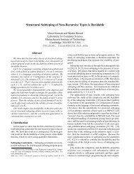
After making a decision, some clauses may become unitclauses. All the unit literals are assigned 1 and the assignmentis propagated until no unit clause exists. All variables assignedas a consequence of implications of a certain decision willhave the same decision level as the decision variable. If aconflict is encountered (i.e. a clause, called conflicting clause,has all its literals assigned value 0), then theanalyze_conflicts() function is called to analyze thereason for the conflict and to resolve it. It also gains someknowledge from the current conflict, and returns abacktracking level so as to resolve this conflict. The returnedbacktracking level indicates the wrong branch decision madepreviously and back_track() will undo the bad branchesin order to resolve the conflict. A zero backtracking levelmeans that a conflict exists even without any branching. Thisindicates that the problem is unsatisfiable. Readers arereferred to [6] for a more detailed discussion of the DPLLalgorithm.There are a large number of different SAT solvers that differmainly in how each of these functions is implemented usingdifferent heuristics. A lot of effort has been spent on decisionmaking(e.g. [13][14][9]), and significant progress has beenmade on how efficient deduction (e.g. [9][15][8]). However,to our knowledge, only [7] and [6] (and its variations) havediscussed implementation of conflict driven learning. Theauthors are not aware of any evaluation of different conflictdriven learning schemes and their influence on theperformance of SAT solvers.while(1) {if (decide_next_branch()) { //Branchingwhile(deduce()==conflict) { //Deducingblevel = analyze_conflicts(); //Learningif (blevel == 0)return UNSATISFIABLE;else back_track(blevel); //Backtracking}}else //no branch means all variables got assigned.return SATISFIABLE;}Figure 1. DPLL with Learning1.2 Implication GraphThe implication relationships of variable assignments duringthe SAT solving process can be expressed as an implicationgraph. A typical implication graph is illustrated in Figure 2.An implication graph is a directed acyclic graph (DAG). Eachvertex represents a variable assignment. A positive variablemeans it is assigned 1; a negative variable means it is assigned0. The incident edges of each vertex are the reasons that leadto the assignment. We will call the vertices that have directededges to a certain vertex as its antecedent vertices. A decisionvertex has no incident edge. Each variable has a decision levelassociated with it, denoted in the graph as a number withinparenthesis. In an implication graph with no conflict there is atmost one vertex for each variable. A conflict occurs whenthere is vertex for both the 0 and the 1 assignment of avariable. Such a variable is referred to as the conflictingvariable. In Figure 2, the variable V 18 is the conflictingvariable. In future discussion, when referring to an implicationgraph, we will only consider the connected component that hasthe conflicting variable in it. The rest of the implication graphis not relevant for the conflict analysis.DecisionVariable-V 6 (1)V 11 (5)-V 13 (2)-V 12 (5)-V 2 (5)V 16 (5)V 4 (3)Conflicting Clause: (V 3 ’+V 19 ’+V 18 ’)-V 10 (5)UIPV 19 (3)V 8 (2)V 1 (5)V 3 (5)-V 5 (5)Figure 2. A typical implication graph-V 17 (1)V 18 (5)ConflictingVariable-V 18 (5)In an implication graph, vertex a is said to dominate vertex biff any path from the decision variable of the decision level ofa to b needs to go through a. A Unique Implication Point(UIP) [6] is a vertex at the current decision level thatdominates both vertices corresponding to the conflictingvariable. For example, in Figure 2, in the sub-graph of currentdecision level 5, V 10 dominates both vertices V 18 and -V 18 ,therefore, it is a UIP. The decision variable is always a UIP.Note that there may be more than one UIP for a certainconflict. In the example, there are three UIPs, namely, V 11 , V 2and V 10 . Intuitively, a UIP is the single reason that implies theconflict at current decision level. We will order the UIPsstarting from the conflict. In the previous example, V 10 is thefirst UIP.In actual implementations, the implication graph is maintainedby associating each assigned non-decision (i.e. implied)variable with a pointer to its antecedent clause. Theantecedent clause of a non-decision variable is the clause thatwas unit at the time when the implication happened, andforced the variable to assume a certain value. By following theantecedent pointers, the implication graph can be constructedwhen needed.1.3 Conflict Analysis and LearningConflict analysis is the procedure that finds the reason for aconflict and tries to resolve it. It tells the SAT solver that thereexists no solution for the problem in a certain search space,and indicates a new search space to continue the search.

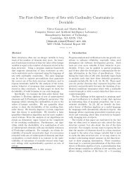
The original DPLL algorithm proposed the simplest conflictanalysis method. For each decision variable, the solver keeps aflag indicating whether it has been tried in both phases or not.When a conflict occurs, the conflict analysis procedure looksfor the decision variable with the highest decision level thathas not been flipped, marks it flipped, undoes all theassignments between that decision level and current decisionlevel, and then tries the other phase for the decision variable.This naïve conflict analysis method actually works well forrandomly generated problems, possibly because randomproblems do not have structure, and learning from a certainpart of the search space will generally not help searches inother parts.More advanced conflict analysis relies on the implicationgraph to determine the actual reasons for the conflict. Thiskind of conflict directed backjumping [7] could back up morethan one level of the decision stack. Thus, it is also called nonchronologicalbacktracking. At the same time, the conflictanalysis engine will also add some clauses to the database.This process is called learning. Such learned clauses arecalled conflict clauses as opposed to conflicting clauses,which refer to clauses that cause the conflict. The conflictclauses record the reasons deduced from the conflict to avoidmaking the same mistake in the future search. These clausesstate that certain combinations of variable assignments are notvalid because they will force the conflicting variable to assumeboth the value 0 and 1, thus leading to a conflict.-V 6 (1)V 11 (5)ReasonSide-V 13 (2)-V 12 (5)-V 2 (5)V 16 (5)Cut 3: cut does notinvolve conflictV 4 (3)-V 10 (5)V 8 (2)V 1 (5)V 3 (5)-V 5 (5)-V 17 (1)V 18 (5)ConflictSide-V 18 (5)Cut 2 Cut 1V 19 (3)Figure 3. Cuts in the implication graph can be added as clausesA conflict clause is generated by a bipartition of theimplication graph. The partition has all the decision variableson one side (called reason side), and the conflicting variablein the other side (the conflict side). All the vertices on thereason side that have at least one edge to the conflict sidecomprise the reason for the conflict. We will call such abipartition a cut. Different cuts correspond to differentlearning schemes. For example, in Figure 3, clause (V 1 ’+ V 3 ’+ V 5 + V 17 + V 19 ’) can be added as a conflict clause, whichcorresponds to cut 1. Similarly, cut 2 corresponds to clause(V 2 + V 4 ’ + V 8 ’ + V 17 + V 19 ’).We will generalize the UIP concept for decision levels otherthan the current level in the context of a partition. We will callvertex a at decision level dl a UIP iff any path from thedecision variable of dl to the conflicting variable needs toeither go through a, or go through a vertex of decision levelhigher than dl that is on the reason side of the partition. Notethat in this definition, the UIP vertices for a certain decisionlevel are determined by the partition of the vertices in decisionlevels higher than it. This is unlike the UIPs for the current(i.e. highest) decision level. Also note that the decisionvariables are UIPs regardless of the partition taken. As in thecase of current decision level UIPs, we will order these UIPsstarting from the conflicting variable as well.As mentioned before, each non-decision variable has anantecedent clause that represents the reason for theassignment. The antecedent clause is represented in theimplication graph as the incoming edges of a vertex. Forexample, in Figure 3, the vertex –V 2 has two incident edges,from –V 12 and V 16 respectively. Therefore, the antecedentclause for V 2 is (V 16 ’ + V 12 + V 2 ’). This clause is alreadypresent in the clause database. We can construct additionalclauses that are consistent with the clause database byreplacing certain literals in the antecedent clause with all oftheir antecedent literals. For example, in the above mentionedclause, if we replace V 16 ’ and V 12 with their antecedentliterals, we get the clause (V 2 ’ + V 6 + V 11 ’ + V 13 ). In Figure 3,this corresponds to cut 3. We will call this kind of replacementa cut not involving conflicts. This clause can be used as alearned clause and be added to the database. However, for thiskind of learning to be useful, there must exist somereconvergence in the part of the graph that is involved in thelearning. Otherwise if the involved part of the graph is a treestructure, then all the information in the learned clause willalready be present in the original database, and the learnedclause will not be useful.The learning process plays a very important role in pruningthe search space of SAT problems. Some state-of-the-art SATsolvers, (e.g. [9]), utilize a technique called random restarts[16] to help the solver from falling into difficult search regionsbecause of bad decisions in the early decision stages. Randomrestarting periodically undoes all the decisions and restarts thesearch from the very beginning. As noted in [12], frequentrestarting actually does not hurt the solving process even forthe unsatisfiable instances. The knowledge of the searchedspace is already recorded in the learned clauses. Therefore,discarding all the searched spaces and restarting is not a wasteof the previous effort as long as the recorded clauses are stillpresent.2. Different Learning Schemes

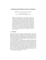
In this section, we will take a look at different learningschemes employed in the existing SAT solvers, and proposesome new schemes based on different cuts of the implicationgraph.Rel_sat [7] is one of the first SAT solvers to incorporatelearning and non-chronological backtracking. The rel_satconflict analysis engine generates the conflict clause byrecursively resolving the conflicting clause with its antecedent,until the resolved clause includes only decision variables ofthe current decision level and variables assigned at decisionlevels smaller than the current level.In the implication graph representation, the rel_sat engine willput all variables assigned at the current decision level, exceptfor the decision variable, on the conflict side; and put all thevariables assigned prior to the current level and the currentdecision variable on the reason side. In our example, theconflict clause added would be:(V 11 ’+ V 6 + V 13 + V 4 ’+ V 8 ’ + V 17 + V 19 ’)We will call this learning scheme rel_sat scheme.ReasonSide-V 6 (1)V 11 (5)-V 13 (2)-V 12 (5)V 16 (5)Cut 3: cut does notinvolve conflictV 4 (3)V 8 (2)V 1 (5)V 3 (5)-V 2 (5) -V 10 (5)ConflictSide-V 5 (5)Figure 4. Different cuts-V 17 (1)V 18 (5)-V 18 (5)First UIP CutV 19 (3)Last UIP CutBy adding a conflict clause, the reason for the conflict isstated. The maximum decision level of the variables (exceptthe current decision level variable) in this conflict clause is thedecision level to backtrack. After backtracking, the conflictclause will become a unit clause, and since the currentdecision variable is the unit literal, it is forced to flip. Such aclause that causes a flip of the variable is called an assertingclause. It is always desirable for a conflict clause to be anasserting clause. The unit variable in the asserting clause willbe forced to assume a value and take the search to a new spaceto resolve the current conflict. To make a conflict clause anasserting clause, the partition needs to have one UIP of thecurrent decision level on the reason side, and all verticesassigned after this UIP on the conflict side. Thus, afterbacktracking, the UIP vertex will become a unit literal, andmake the clause an asserting clause.Another learning scheme is implemented in GRASP [6].GRASP’s learning scheme is different from rel_sat’s in thesense that it tries to learn as much as possible from a conflict.There are two cases when a conflict occurs in GRASP’slearning engine. If the current decision variable is a realdecision variable (explained later), the GRASP learningengine will add each reconvergence between UIPs in currentdecision level as a learned clause. In our example, if V 11 is areal decision (i.e. it has no antecedent), when the conflictoccurs, the GRASP engine will add one clause into thedatabase corresponding to the UIP reconvergences shown inFigure 4. This corresponds to the clause (V 2 ’ + V 6 + V 11 ’ +V 13 ).Moreover, GRASP will also include a conflict clause thatcorresponds to the partition where all the variables assigned atthe current decision level after the first UIP will be put on theconflict side. The rest of the vertices will be put on the reasonside. This corresponds to the FirstUIP cut as shown in figure3. The clause added will be (V 10 + V 8 ’ + V 17 + V 19 ’).After backtracking, the conflict clause will be an assertingclause, which forces V 10 to flip. Note that V 10 was not adecision variable before. In GRASP, such a decision is a fakedecision. The decision level of V 10 remains unchanged. Thisessentially means that we are not done at the current decisionlevel yet. We will call this mode of the analysis engine flipmode.If the deduction found that flipping the decision variable stillleads to a conflict, the GRASP conflict analysis engine willenter backtracking mode. Besides the clauses that have to beadded in the flip mode, it also adds another clause called theback clause. The cut for the back clause will put all thevertices at the current decision level (including the fakedecision variable) on the conflict side, and all other vertices onthe reason side. For our example, suppose the decisionvariable V 11 is actually a fake decision variable, withantecedent clause (V 21 + V 20 + V 11 ’). Then, besides the twoclauses added before, the GRASP engine will add anotherclause(V 21 + V 20 + V 6 + V 13 + V 4 ’ + V 8 ’ + V 17 + V 19 ’)This clause is a conflicting clause, and it only involvesvariables assigned before the current decision level. Theconflict analysis engine will continue to resolve this conflict,and bring the solver to an earlier decision level. We will callthis learning scheme the GRASP scheme.Besides these two learning schemes, many more options exist.One obvious learning scheme is to add only the decisionvariables involved in the conflict to the conflict clause. In ourimplication graph representation, this corresponds to makingthe cut such that only the decision variables are in the reasonside, and all the other variables are in the conflict side. Wewill call this scheme Decision scheme. Note that it is no goodto include all the decision variables of the current search treein the conflict clause, because such a combination of decisions

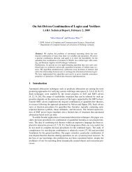
DecisionStrategySDISVMicroprocessor Formal Verification[19] Bounded Model Checking [18]fvp-unsat.1.0(4) sss.1.0(48) sss.1.0a(9) barrel (8) longmult(16) queueinvar(10) satplan(20)1uip 532.8 24.56 10.63 1012.62 2887.11 6.58 39.342uip 746.87 27.32 16.96 641.64 2734.57 16.37 41.373uip 2151.26 69.12 47.66 656.56 2946.73 19.44 57.16alluip 0.68(3) 1746.27(2) 79.09 1081.57(1) 11160.25 18.07 71.86rel_sat 2034.09 193.93 82.51 292.33(1) 5719.73 14.4 96.61mincut 1612.74(2) 2293.18 11.15 4119.34(1) 7321.69(5) 100.94 43.84grasp 2224.44 94.64 33.99 654.54 6196.82 97.82 309.03decision* 0(4) 1022.57(17) 227.37(3) 541.96(2) 1421.35(4) 334.39(4) 193.36(3)1uip_f 11.36(3) 15307.13(3) 2997.37 281.48(1) 3141.8 817.07(5) 18(2)2uip_f 23.07(3) 18844.51(3) 2646.99 344.34(1) 4279.07 777.2(5) 29.51(2)3uip_f 40.75(3) 3985.23(9) 4109.86 432.77(1) 4440.49 860.3(5) 37.62(2)alluip_f 0(4) 4063.44(25) 0.28(8) 699.42(1) 11375.32 2025.08(5) 1136.44(2)relsat_f 80.94(3) 3114.83(16) 4261.25(4) 293.09(1) 4396.73 478.37(6) 3323.71(3)mincut_f 0(4) 5619.4(15) 590.79(4) 3408.28(1) 5232.69(5) 3206.36(4) 373.78(2)grasp_f 22.51(3) 6497.99(8) 3382.47 326.46(1) 5597.1 792.12(5) 149.8(2)decision_f* 0(4) 415.76(42) 40.57(8) 479.61(1) 1006.58(6) 1.27(8) 600.87(10)* timeout set to 600s instead of 3600sDEXIFTable 1. Run time for different learning schemeswill never occur again in the future unless we restart. Thus thelearned clause will hardly help prune any search space at all.The decision variables are the last UIPs for each decisionlevel. A more careful study of the Decision scheme suggestsmaking a partition not limited at decision variables, but afterany UIPs of each of the decision levels. One of the choices isto make a partition after the first UIP of each decision level.We will call this scheme the All UIP scheme. Because UIPs ofa lower level depend on the partition, we need to do thepartition from the current decision level up to decision level 1.More precisely, the solver needs to find the first UIP of thecurrent decision level, then all variables of current decisionlevel assigned after it that have a path to the conflictingvariable will be on the conflict side; the rest will be on thereason side. Then the solver will proceed to the decision levelprior to current one, and so on, until reaching decision level 1.Another learning scheme is to make the conflict clause assmall as possible. This corresponds to the problem that givenan implication graph, remove the smallest number of variables(may include decision variables, but not the conflictingvariable) from the implication graph so that there exist no pathfrom the decision variables to the conflicting variable. This isa typical vertex min-cut problem, which can be transformedinto an edge min-cut problem and solved with maxflowmincutalgorithms.It may also be desirable to make the conflict clause as relevantto the current conflict as possible. Therefore, we may want tomake the partition closer to the conflicting variable. As wementioned earlier, to make the conflict clause an assertingclause, we need to put one UIP of the current decision level onthe reason side. Therefore, if we put all variables assignedafter the first UIP of current decision level that have paths tothe conflicting variable on the conflict side, and everythingelse on the reason side, we get a partition that is as close to theconflict as possible. We will call this 1 UIP scheme.The 1 UIP scheme is different from the All UIP scheme in thatwe only require the current decision level have its first UIP atthe reason side just before the partition. We may also requirethat the immediately previous decision level have its first UIPon the reason side just before the partition. This will make theconflict have only one variable that was assigned at theimmediate previous decision level. We will call this the 2 UIPscheme, similarly, we can have 3 UIP scheme etc., up to AllUIP, which makes the conflict clause have only one variablefor any decision level involved.Other than the min-cut scheme, all the other above-mentionedlearning schemes can be implemented by a traversal of theimplication graph. The time complexity of the traversal isO(V+E). Here V and E are the number of vertices and edgesof the implication graph respectively. The time complexity forfinding a min-cut of the implication graph can be implementedin O(VElg(V 2 /E)) time [17].A good learning scheme should reduce the number ofdecisions needed to solve certain problems as much aspossible. The effectiveness of a learning scheme is very hardto determine a priori. Generally speaking, a shorter clause

9vliw_bp_mc( unsat, 19148 vars )longmult10( unsat, 4852 vars )sat/bw_large.d.cnf( sat, 6325 vars )1UIP rel_sat GRASP 1UIP rel_sat GRASP 1UIP rel_sat GRASPBranches(x10e6) 1.91 4.71 1.07 0.13 0.19 0.12 0.019 0.046 0.027Added Clauses(x10e6) 0.18 0.76 1.06 0.11 0.17 0.36 0.011 0.030 0.071Added Literals (x10e6) 73.13 292.08 622.96 17.16 28.07 77.47 0.56 1.61 6.12Added lits/cls 405.08 384.31 587.41 150.17 162.96 213.43 50.87 52.94 86.19Num. Implications(x10e6) 69.85 266.21 78.49 71.72 108.00 74.83 7.23 17.84 16.81Runtime 522.26 1996.73 2173.14 339.99 612.64 762.94 23.44 52.64 124.13Table 2. Detailed information on three large test cases for three learning schemes using VSIDS branching heuristiccontains more information than a longer clause. Therefore, acommon belief is that the shorter the learned clause, the moreeffective the learning scheme. However, SAT solving is adynamic process. It has complex interplay between thelearning schemes and the search process. Therefore, theeffectiveness of certain searching schemes can only bedetermined by empirical data for the entire solution process.3. Experimental Results and DiscussionsIn this section, we empirically compare the learning schemesdiscussed in previous sections. We have implemented all theabove-mentioned learning schemes in the SAT solver zChaff(an independent implementation that shares several featureswith the Chaff SAT solver [9]). zChaff utilizes the highlyoptimized Chaff Boolean Constraint Propagation (BCP)engine and VSIDS decision heuristic, thus making theevaluation more interesting because some large benchmarkscan be evaluated in reasonable amount of time.zChaff’s default branching scheme VSIDS depends on theadded conflict clauses and literal counts for making branchingdecisions. Therefore, different learning schemes may alsoaffect the decision strategy. To make a fair comparison, wealso implemented a fixed branching strategy, which willbranch on the first unassigned variable with the smallestvariable index. The variables indices are predetermined for agiven problem instance. Default values are used for all othersettings.Our test suite consists of benchmarks from bounded modelchecking [18] and microprocessor formal verification [19].We also included a benchmark from the AI planningcommunity to cover a wider range of applications. Theexperiments were conducted on dual Pentium III 833Mhzmachines running Linux, with 2G bytes physical memory.Each CPU has 32k L1 cache and 256k L2 cache. The time outlimit for each SAT instance is 3600 seconds. For the Decisionlearning scheme, because of the large number of aborts, thetime out limit was set to 600 seconds to reduce totalexperiment time.The run times of different learning schemes on thebenchmarks are shown in Table 1. Each benchmark class hasmultiple instances, shown in the parentheses following eachbenchmark name. In the result section, the times shown are thetotal time spent on the solved instances only. The number ofaborted instances is shown in the parentheses following runtime. If there is no such number, all the instances are solved.For example, fvp-unsat-1.0 has 4 instances. Using the defaultVSIDS decision strategy, the min-cut learning scheme took1612.74 seconds to solve two of them, and aborted on theother two.From the experiment data we can see that for both default andfixed branching heuristics, the 1UIP learning scheme clearlyoutperforms other learning schemes. Contrary to generalbelief, the decision schemes that generate small clauses, e.g.min-cut, all UIP and Decision do not perform as well.We selected the best of our proposed schemes, i.e. the 1UIPscheme, and compared it with the learning schemes employedin other state-of-the-art SAT solvers, i.e. the GRASP schemeand the rel_sat scheme. We selected three difficult test casesfrom three classes of the benchmark suites. Detailed solverstatistics for these schemes are presented in Table 2. Thebranching heuristic employed was VSIDS. From this table wefind that the results are quite interesting. As we mentionedbefore, the GRASP scheme tries to learn as much as possiblefrom conflicts. Actually, it will learn more than one clause foreach conflict. For a given conflict, the clause leaned by 1UIPscheme is actually also learned by the GRASP scheme.Therefore, in most of the cases, the GRASP scheme needs asmaller number of branches to solve the problem. However,because the GRASP scheme records more clauses, the BCPprocess is slowed down. Therefore, the total run time of theGRASP scheme is more than 1UIP scheme. On the other hand,though rel_sat and 1UIP both learn one clause for eachconflict, the learned clause of rel_sat scheme is not aseffective as 1UIP as it needs more branches.4. Conclusions and Future ResearchThis paper explores the conflict driven learning techniqueswidely used in current state-of-the-art Boolean satisfiabilitysolvers. We have examined the strength and weaknesses ofcurrent learning schemes employed in various SAT solvers.

We have generalized conflict driven learning into a problemof partitioning the implication graph, and have proposed somenew learning schemes. These learning schemes wereimplemented in the SAT solver zChaff and extensiveexperiments were conducted. We have found that differentlearning schemes can affect the behavior of the SAT solversignificantly. The learning scheme based on the first UniqueImplication Point of the implication graph has proved to bequite robust and effective in solving SAT problems incomparison with other schemes.For future research, it would be interesting to explore thepossibility of mixing different learning schemes in a single runof the SAT solving process. As the SAT solving processprogresses, the number of literals in the learned clauses growsquickly. For some of the problems, in the later stages of thesolving process each learned clause may have severalthousand literals. The clause database may become tens oftimes larger than the original size; very quickly making thesolving process memory limited. It would be interesting toexplore the possibility of using different learning schemesduring different stages of the solution process. This can lead tobetter control of the size of the learned clause.As pointed out before, learning is very important to thesuccess of the SAT solvers, but there is still little work onlearning in current research of SAT solving algorithms. Infact, there is very little insight about why learning is useful andwhat makes one learning scheme better than the other. Forexample, relevance based learning and clause length boundedlearning are common practices in current SAT algorithms, butnot much attention has been given to choosing optimalparameters for different problems. As SAT based methodsbecomes more and more popular in a wide range ofapplications, it is increasingly important for us to answer thesequestions in a systematic way. This paper represents a step inthat direction.5. REFERENCES[1] P. Stephan, R. K. Brayton, and A. Sangiovanni-Vincentelli, “Combinational Test Generation UsingSatisfiability,” IEEE Transactions on Computer-AidedDesign of Integrated Circuits and Systems, vol. 15, 1167-1176, 1996.[2] M. Velev, and R. Bryant, “Effective Use of BooleanSatisfiability Procedures in the Formal Verification ofSuperscalar and VLIW Microprocessors,” Proceedings ofthe Design Automation Conference, July 2001.[3] A. Biere, A. Cimatti, E. M. Clarke, and Y. Zhu. “SymbolicModel Checking without BDDs,” Tools and Algorithms forthe Analysis and Construction of Systems (TACAS'99),number 1579 in LNCS. Springer-Verlag, 1999.)[4] B. Selman, H. Kautz, and B. Cohen. “Local SearchStrategies for Satisfiability Testing.” DIMACS Series inDiscrete Mathematics and Theoretical Computer Science,vol. 26, AMS, 1996.[5] J. W. Freeman, “Improvements to PropositionalSatisfiability Search Algorithms,” Ph.D. Dissertation,Department of Computer and Information Science,University of Pennsylvania, May 1995.[6] J. P. Marques-Silva and K. A. Sakallah, “GRASP: ASearch Algorithm for Propositional Satisfiability,” IEEETransactions on Computers, vol. 48, 506-521, 1999.[7] R. Bayardo, and R. Schrag, “Using CSP look-backtechniques to solve real-world SAT instances,” Proceedingsof the 14th Nat. (US) Conf. on Artificial Intelligence (AAAI-97), AAAI Press/The MIT Press, 1997.[8] H. Zhang. “SATO: An efficient propositional prover,”Proceedings of the International Conference on AutomatedDeduction, July 1997.[9] M. Moskewicz, C. Madigan, Y. Zhao, L. Zhang, and S.Malik. “Chaff: Engineering an efficient SAT Solver,”Proceedings of the Design Automation Conference, July2001.[10] M. Davis, G. Logemann, and D. Loveland. “A machineprogram for theorem proving.,” Communications of theACM, (5):394-397, 1962.[11] G. Stalmarck, “A system for determining prepositionallogic theorems by applying values and rules to triplets thatare generated from a formula,” Technical report, EuropeanPatent N 0403 454 (1995), US Patent N 5 27689.[12] M. Moskewicz, L. Zhang, Y. Zhao, S. Malik and C.Madigan, “Chaff: A Fast SAT Solver for EDAApplications”, Presented at the Dagstuhl seminar on SATv.s. BDD, March 2001. Dagstuhl, Germany.[13] J. P. Marques-Silva, “The Impact of Branching Heuristicsin Propositional Satisfiability Algorithms,” Proceedings ofthe 9th Portuguese Conference on Artificial Intelligence(EPIA), September 1999.[14] Chu Min Li and Anbulagan, “Heuristics based on unitpropagation for satisfiability problems,” Proceedings of thefifteenth International Joint Conference on ArtificialIntelligence (IJCAI’97), Pages 366-371, Nagoya (Japan),1997[15] Chu Min Li, “Integrating equivalency reasoning intoDavis-Putnam Procedure,” Proceedings of AAAI 2000,2000.[16] C. P. Gomes, B. Selman, and H. Kautz, “BoostingCombinatorial Search Through Randomization”,Proceedings of AAAI-98, Madison, WI, 1998.[17] A. Goldberg, R. Tarjan. “A new approach to themaximum flow problem,” Proceedings of the eighteenthannual ACM Symposium on Theory of Computing, 1986.[18] Bounded Model Checking benchmarks available athttp://www.cs.cmu.edu/~modelcheck/bmc/bmcbenchmarks.html[19] M. N. Velev, Microprocessor Formal VerificationBenchmarks, available at http://www.ece.cmu.edu/~mvelev