SExtractor Draft - METU Astrophysics

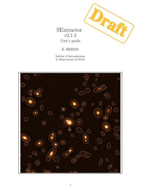
1DraftSExtractorv2.1.3User’s guideE. BERTINInstitut d’Astrophysique& Observatoire de Paris

3Contents1 What is SExtractor? 52 Installing the software 52.1 Software and hardware requirements . . . . . . . . . . . . . . . . . . . . . . . . . 52.2 Obtaining SExtractor . . . . . . . . . . . . . . . . . . . . . . . . . . . . . . . . . 62.3 Installation . . . . . . . . . . . . . . . . . . . . . . . . . . . . . . . . . . . . . . . 63 Using SExtractor 63.1 Syntax . . . . . . . . . . . . . . . . . . . . . . . . . . . . . . . . . . . . . . . . . . 63.2 The configuration file . . . . . . . . . . . . . . . . . . . . . . . . . . . . . . . . . . 63.2.1 Format . . . . . . . . . . . . . . . . . . . . . . . . . . . . . . . . . . . . . 63.2.2 Configuration parameter list . . . . . . . . . . . . . . . . . . . . . . . . . 73.3 The catalog parameter file . . . . . . . . . . . . . . . . . . . . . . . . . . . . . . . 113.3.1 Format . . . . . . . . . . . . . . . . . . . . . . . . . . . . . . . . . . . . . 113.4 Example of configuration . . . . . . . . . . . . . . . . . . . . . . . . . . . . . . . 124 Overview of the software 125 Handling of image data 126 Detection and segmentation 126.1 Background estimation . . . . . . . . . . . . . . . . . . . . . . . . . . . . . . . . . 146.1.1 Configuration parameters and tuning . . . . . . . . . . . . . . . . . . . . . 156.1.2 CPU cost . . . . . . . . . . . . . . . . . . . . . . . . . . . . . . . . . . . . 156.2 Filtering . . . . . . . . . . . . . . . . . . . . . . . . . . . . . . . . . . . . . . . . . 166.2.1 Convolution . . . . . . . . . . . . . . . . . . . . . . . . . . . . . . . . . . . 166.2.2 Non-linear filtering . . . . . . . . . . . . . . . . . . . . . . . . . . . . . . . 176.2.3 What is filtered, and what isn’t . . . . . . . . . . . . . . . . . . . . . . . . 176.2.4 Image boundaries and bad pixels . . . . . . . . . . . . . . . . . . . . . . . 186.2.5 Configuration parameters. . . . . . . . . . . . . . . . . . . . . . . . . . . . 186.2.6 CPU cost. . . . . . . . . . . . . . . . . . . . . . . . . . . . . . . . . . . . . 186.2.7 Filter file formats. . . . . . . . . . . . . . . . . . . . . . . . . . . . . . . . 186.3 Thresholding . . . . . . . . . . . . . . . . . . . . . . . . . . . . . . . . . . . . . . 196.3.1 Configuration parameters. . . . . . . . . . . . . . . . . . . . . . . . . . . . 196.4 Deblending . . . . . . . . . . . . . . . . . . . . . . . . . . . . . . . . . . . . . . . 20

47 Weighting 227.1 Weight-map formats . . . . . . . . . . . . . . . . . . . . . . . . . . . . . . . . . . 227.2 Weight threshold . . . . . . . . . . . . . . . . . . . . . . . . . . . . . . . . . . . . 237.3 Effect of weighting . . . . . . . . . . . . . . . . . . . . . . . . . . . . . . . . . . . 237.4 Combining weight maps . . . . . . . . . . . . . . . . . . . . . . . . . . . . . . . . 247.5 Interpolation . . . . . . . . . . . . . . . . . . . . . . . . . . . . . . . . . . . . . . 248 Flags 248.1 Internal flags . . . . . . . . . . . . . . . . . . . . . . . . . . . . . . . . . . . . . . 258.2 External flags . . . . . . . . . . . . . . . . . . . . . . . . . . . . . . . . . . . . . . 259 Measurements 259.1 Positional parameters derived from the isophotal profile . . . . . . . . . . . . . . 269.1.1 Limits: XMIN, YMIN, XMAX, YMAX . . . . . . . . . . . . . . . . . . . . . . . . 269.1.2 Barycenter: X, Y . . . . . . . . . . . . . . . . . . . . . . . . . . . . . . . . 269.1.3 Position of the peak: XPEAK, YPEAK . . . . . . . . . . . . . . . . . . . . . . 279.1.4 2nd order moments: X2, Y2, XY . . . . . . . . . . . . . . . . . . . . . . . . 279.1.5 Basic shape parameters: A, B, THETA . . . . . . . . . . . . . . . . . . . . . 279.1.6 Ellipse parameters: CXX, CYY, CXY . . . . . . . . . . . . . . . . . . . . . . . 289.1.7 By-products of shape parameters: ELONGATION, ELLIPTICITY . . . . . . . 299.1.8 Position errors: ERRX2, ERRY2, ERRXY, ERRA, ERRB, ERRTHETA, ERRCXX,ERRCYY, ERRCXY . . . . . . . . . . . . . . . . . . . . . . . . . . . . . . . . . 299.1.9 Handling of “infinitely thin” detections . . . . . . . . . . . . . . . . . . . 309.2 Astrometry and WORLD coordinates . . . . . . . . . . . . . . . . . . . . . . . . . . 319.2.1 Angular coordinates . . . . . . . . . . . . . . . . . . . . . . . . . . . . . . 319.2.2 Use of the FITS keywords for astrometry . . . . . . . . . . . . . . . . . . 329.3 Cross-identification within SExtractor . . . . . . . . . . . . . . . . . . . . . . . . 329.3.1 The ASSOC list . . . . . . . . . . . . . . . . . . . . . . . . . . . . . . . . . 329.3.2 Controlling the ASSOC process . . . . . . . . . . . . . . . . . . . . . . . . . 329.3.3 Output from ASSOC . . . . . . . . . . . . . . . . . . . . . . . . . . . . . . . 33A Appendices 35A.1 FAQ (Frequently Asked Questions) . . . . . . . . . . . . . . . . . . . . . . . . . . 35

51 What is SExtractor?SExtractor (Source-Extractor) is a program that builds a catalogue of objects from an astronomicalimage. It is particularly oriented towards reduction of large scale galaxy-survey data,but it also performs well on moderately crowded star fields. Its main features are:• Simplicity of usage and configuration.• Speed: typically 500 kpixel/s with a Pentium2@450MHz.• Ability to work with very large images (up to 65k × 65k pixels on 32bit machines, or2G × 2G pixels on 64bit machines), thanks to buffered image access.• Robust deblending of overlapping extended objects.• Real-time filtering of images to improve detectability.• Neural-Network-based star/galaxy classifier.• Flexible catalogue output of desired parameters only.• Pixel-to-pixel photometry in dual-image mode.• Handling of weight-maps and flag-maps.• Optimum handling of images with variable S/N.• Special mode for photographic scans.• Modularity of the code that enables one to implement new parameters.The purpose of SExtractor was to find a compromise between refinement in both detection andmeasurements, and computational speed.2 Installing the software2.1 Software and hardware requirementsSince the beginning in 1993, the development of SExtractor was always made on Unix systems(successively: SUN-OS, HP/UX, SUN-Solaris, Digital Unix and GNU/Linux). Successful portsby external contributors have been reported on non-Unix OSes such as AMIGA-OS, DEC-VMSand even MS-DOS Windows95 1 and NT ; ). They are however not currently supported by theauthor, and Unix remains the recommended system for running SExtractor. The software isgenerally run in (ANSI) text-mode from a shell. A window system is therefore unnecessary withpresent versions.On the hardware side, memory requirements obviously depend on the size of the images to beprocessed. But to give an idea, a typical processing of 1024 × 1024 pixel images should requireno more than 8 MB of silicon memory. For very large images, (32000 × 32000 pixels or more), aminimum of 200MB is recommended. Swap-space can of course be put to contribution, althougha strong performance hit is to be expected.1 Binaries are available on the WWW, see e.g. http://www.tass-survey.org/tass/software/software.html#sextract

62.2 Obtaining SExtractorThe easiest way to obtain SExtractor is to download it from an internet site. The current officialanonymous FTP site is ftp://ftp.iap.fr/pub/from users/bertin/sextractor/. There canbe found the latest versions of the program as standard .tar.gz Unix archives, plus somedocumentation.2.3 InstallationTo install, you must first uncompress and unarchive the archive:gzip -dc sex_2.x.x.tar.gz | tar xvA new directory called sextractor2.x.x should now appear at the current position on yourdisk. You should then just enter the directory and follow the instructions in the file called“INSTALL”.3 Using SExtractor3.1 SyntaxSExtractor is run from the shell with the following syntax:% sex image [-c configuration-file] [ -Parameter1 Value1 ] [ -Parameter2 Value2 ] ...The part enclosed within brackets is optional. Any ”-Parameter Value” statement in thecommand-line overrides the corresponding definition in the configuration-file or any defaultvalue (see below). Actually, two image filenames can be provided, separated by a comma:% sex image1,image2This syntax makes SExtractor run in the so-called “double-image mode”: image1 will be used fordetection of sources, and image2 for measurements only. image1 and image2 must have the samedimensions. Changing image2 for another image will not modify the number of detected sources,neither affect their positional or basic shape parameters. But most photometric parameters,plus a few others, will use image2 pixel values, which allows one to easily measure pixel-to-pixelcolours.3.2 The configuration fileSExtractor needs a configuration file. If no configuration file-name is specified in the commandline, SExtractor tries to load a file called “default.sex” from the local directory.3.2.1 FormatThe format is ASCII. There must be only one parameter set per line, following the form:Config-parameterValue(s)Extra spaces or linefeeds are ignored. Comments must begin with a “#” and end with a linefeed.Values can be of different types: strings (can be enclosed between double quotes), floats, integers,keywords or boolean (Y/y or N/n). Some parameters accept zero or several values, which must

7then be separated by commas. Integers can be given as decimals, in octal form (preceded by digitO), or in hexadecimal (preceded by 0x). The hexadecimal format is particularly convenient forwriting multiplexed bit values such as binary masks. Environment variables, written as $HOMEor ${HOME} are expanded, and not only for string parameters. Some parameters are assigneddefault values in SExtractor and can therefore be omitted from the configuration file; they arelisted in §3.2.2.3.2.2 Configuration parameter listHere is a complete list of all the configuration parameters known to SExtractor. Many of themare just used with default values. Please refer to §?? for a detailed description of their meaning.Parameter default type DescriptionANALYSIS THRESH — floats (n ≤ 2) Threshold (in surface brightness) atwhich CLASS STAR and FWHM operate.1 argument: relative toBackground RMS. 2 arguments: mu(mag.arcsec −2 ), Zero-point (mag).ASSOC DATA 2,3,4 integers (n ≤ 32) Nos of the columns in the ASSOC filethat will be copied to the catalog output.ASSOC NAME sky.list string Name of the ASSOC ASCII file.ASSOC PARAMS 2,3,4 integers (2 ≤ n ≤ 3) Nos of the columns in the ASSOC filethat will be used as coordinates andweight for cross-matching.ASSOC RADIUS 2.0 float Search radius (in pixels) for ASSOC.ASSOC TYPE MAG SUM keyword Method for cross-matching in ASSOC:FIRST– keep values corresponding to thefirst match found,NEAREST– values corresponding to the nearestmatch found,MEAN– weighted-average values,MAG MEAN– exponentialy weighted-average values,SUM– sum values,MAG SUM– exponentialy sum values,MIN– keep values corresponding to thematch with minimum weight,MAX– keep values corresponding to thematch with maximum weight.ASSOCSELEC TYPE MATCHED keyword What sources are printed in the outputcatalog in case of ASSOC:ALL– all detections,MATCHED– only matched detections,-MATCHED – only detections that were notmatched.BACK FILTERSIZE — integers (n ≤ 2) Size, or Width,Height (in backgroundmeshes) of the background-filteringmask.

8BACK SIZE — integers (n ≤ 2) Size, or Width,Height (in pixels) of abackground mesh.BACK TYPE INTERNAL keywords (n ≤ 2) What background is subtracted fromthe images:INTERNAL – the internal interpolatedbackground-map,MANUAL– a user-supplied constant value providedin BACK VALUE.BACK VALUE 0.0,0.0 floats (n ≤ 2) in BACK TYPE MANUAL mode, the constantvalue to be subtracted from theimages.BACKPHOTO THICK 24 integer Thickness (in pixels) of the backgroundLOCAL annulus.BACKPHOTO TYPE GLOBAL keyword Background used to compute magnitudes:GLOBAL– taken directly from the backgroundLOCALmap,– recomputed in a “rectangular annulus”around the object.CATALOG NAME — string Name of the output catalogue. Ifthe name “STDOUT” is given andCATALOG TYPE is set to ASCII,ASCII HEAD, or ASCII SKYCAT, thecatalogue will be piped to thestandard output (stdout)CATALOG TYPE — keyword Format of output catalog:ASCII– ASCII table; the simplest, but spaceand time consuming,– as ASCII, preceded by a header containinginformation about the content,ASCII SKYCAT – SkyCat ASCII format (WCS coordinatesrequired),FITS 1.0 – FITS format as in SExtractor 1,ASCII HEADFITS LDAC – FITS “LDAC” format (the originalimage header is copied).CHECKIMAGE NAME check.fits strings (n ≤ 16) File name for each “check-image”.CHECKIMAGE TYPE NONE keywords (n ≤ 16) Type of information to put in the“check-images”:NONE– no check-image,IDENTICAL – identical to input image (useful forconverting formats),BACKGROUND – full-resolution interpolated backgroundmap,BACKGROUND RMS – full-resolution interpolated backgroundnoise map,MINIBACKGROUND – low-resolution background map,MINIBACK RMS – low-resolution background noisemap,-BACKGROUND – background-subtracted image,FILTERED – background-subtracted filtered image(requires FILTER = Y),

9OBJECTS-OBJECTSAPERTURESSEGMENTATION– detected objects,– background-subtracted image withdetected objects blanked,– MAG APER and MAG AUTO integrationlimits,– display patches corresponding topixels attributed to each object.CLEAN — boolean If true, a “cleaning” of the catalogueis done before being written to disk.CLEAN PARAM — float Efficiency of “cleaning”.DEBLEND MINCONT — float Minimum contrast parameter for deblending.DEBLEND NTHRESH — integer Number of deblending sub-thresholds.DETECT MINAREA — integer Minimum number of pixels abovethreshold triggering detection.DETECT THRESH — floats (n ≤ 2) Detection threshold. 1 argument:(ADUs or relative to Background RM-S, see THRESH TYPE). 2 arguments: µ(mag.arcsec −2 ), Zero-point (mag).DETECT TYPE CCD keyword Type of device that produced the image:CCD– linear detector like CCDs or NIC-MOS,PHOTO– photographic scan.FILTER — boolean If true, filtering is applied to the databefore extraction.FILTER NAME — string Name of the file containing the filterdefinition.FILTER THRESH floats (n ≤ 2) Lower and higher thresholds (in backgroundstandard deviations) for a pixelto be considered in filtering (usedfor retina-filtering only).FITS UNSIGNED N boolean Force 16-bit FITS input data to be interpretedas unsigned integers.FLAG IMAGE flag.fits strings (n ≤ 4) File name(s) of the “flag-image(s)”.FLAG TYPE OR keyword Combination method for flags on thesame object:OR– arithmetical OR,AND– arithmetical AND,MIN– minimum of all flag values,MAX– maximum of all flag values,MOST– most common flag value.GAIN float “Gain” (conversion factor ine − /ADU) used for error estimates ofCCD magnitudes .INTERP MAXXLAG 16 integers (n ≤ 2) Maximum x gap (in pixels) allowed ininterpolating the input image(s).INTERP MAXYLAG 16 integers (n ≤ 2) Maximum y gap (in pixels) allowed ininterpolating the input image(s).

10INTERP TYPE ALL keywords (n ≤ 2) Interpolation method from thevariance-map(s) (or weight-map(s)):NONE– no interpolation,VAR ONLY – interpolate only the variance-map(detection threshold),ALL– interpolate both the variance-mapand the image itself.MAG GAMMA float γ of the emulsion (takes effect inPHOTO mode only).MAG ZEROPOINT float Zero-point offset to be applied to magnitudes.MASK TYPE CORRECT keyword Method of “masking” of neighboursfor photometry:NONE– no masking,BLANK– put detected pixels belonging toCORRECTneighbours to zero,– replace by values of pixels symetricwith respect to the source center.MEMORY BUFSIZE — integer Number of scan-lines in the imagebuffer.Multiply by 4 the frame widthto get equivalent memory space inbytes.MEMORY OBJSTACK — integer Maximum number of objects that theobject-stack can contain. Multiply by300 to get equivalent memory space inbytes.MEMORY PIXSTACK — integer Maximum number of pixels that thepixel-stack can contain. Multiply by16 to 32 to get equivalent memory s-pace in bytes.PARAMETERS NAME — string The name of the file containing the listof parameters that will be computedand put in the catalogue for each object.PHOT APERTURES — floats (n ≤ 32) Aperture diameters in pixels (used byMAG APER).PHOT AUTOPARAMS — floats (n = 2) MAG AUTO controls: scaling parameterk of the 1st order moment, and minimumR min (in units of A and B).PHOT AUTOAPERS 0.0,0.0 floats (n = 2) MAG AUTO minimum (circular) aperturediameters: estimation disk, andmeasurement disk.PHOT FLUXFRAC 0.5 floats (n ≤ 32) Fraction of FLUX AUTO defining eachelement of the FLUX RADIUS vector.PIXEL SCALE — float Pixel size in arcsec (for surfacebrightness parameters, FWHM and s-tar/galaxy separation only).SATUR LEVEL — float Pixel value above which it is consideredsaturated.SEEING FWHM — float FWHM of stellar images in arcsec (onlyfor star/galaxy separation).

11FULLSTARNNW NAME — string Name of the file containing the neuralnetworkweights for star/galaxy separation.THRESH TYPE RELATIVE keywords (n ≤ 2) Meaning of the DETECT THRESH andANALYSIS THRESH parameters :RELATIVE – scaling factor to the backgroundRMS,ABSOLUTE – absolute level (in ADUs or in surfacebrightness).VERBOSE TYPE NORMAL keyword How much SExtractor comments itsoperations:QUIET– run silently,NORMAL– display warnings and limited infoconcerning the work in progress,EXTRA WARNINGS – like NORMAL, plus a few more warningsif necessary,– display a more complete informationand the principal parameters of all theobjects extracted.WEIGHT GAIN Y boolean If true, weight maps are considered asgain maps.WEIGHT IMAGE weight.fits strings (n ≤ 2) File name of the detection and measurement“weight-image”, respectively.WEIGHT TYPE NONE keywords (n ≤ 2) Weighting scheme (for single image, ordetection and measurement images):NONEBACKGROUNDMAP RMSMAP VARMAP WEIGHT– no weighting,– variance-map derived from the imageitself,– variance-map derived from an externalRMS-map,– external variance-map,– variance-map derived from an externalweight-map,3.3 The catalog parameter fileIn addition to the configuration file detailed above, SExtractor needs a file containing the list ofparameters that will be listed in the output catalog for every detection. This allows the softwareto compute only catalog parameters that are needed. The name of this catalog-parameter fileis traditionally suffixed with .param, and must be specified using the PARAMETERS NAME configparameter.3.3.1 FormatThe format of the catalog parameter list is ASCII, and there must be only one keyword perline. Presently two kinds of keywords are recognized by SExtractor: scalars and vectors. S-calars, like X IMAGE, yield single numbers in the output catalog. Vectors, like MAG APER(4) or1 Optional parameter

12VIGNET(15,15), yield arrays of numbers. The order in which the parameters will be listed inthe catalogue are the same as that of the keywords in the parameter list. Comments are allowed,they must begin with a “#”. Here is a descriptive list of available parameter keywords.3.4 Example of configuration4 Overview of the softwareThe complete analysis of an image is done in two passes through the data. During the firstpass, a model of the sky background is built, and a couple of global statistics are estimated.During the second pass, the image is background-subtracted, filtered and thresholded “on-thefly”.Detections are then deblended, pruned (“CLEANed”), photometered, classified and finallywritten to the output catalog. Let’s now enter a little more into the details of each of theseoperations 2 .5 Handling of image dataSExtractor accepts images stored in FITS 3 format (Wells et al. 1981, see also http://fits.gsfc.nasa.gov).Currently, only “Basic FITS” images are recognized. For images with NAXIS > 2, only the firstdata-plane is loaded. Extensions are ignored. If WCS 4 information (Greisen & Calabretta 1995,http://www.cv.nrao.edu/fits/documents/wcs/wcs.all.ps) is available in the header, it isautomatically used by SExtractor to compute astrometric parameters. Other astrometric descriptionslike AST (Starlink format) or the solution coefficients of the DSS 5 plates are notrecognized by the software.In SExtractor, as in all similar programs, FITS axis “1” is traditionaly refered as the X axis,and FITS axis “2” as the Y axis.6 Detection and segmentationIn SExtractor, the detection of sources is part of a process called segmentation in the imageprocessingvocabulary. Segmentation normally consists of identifying and separating imageregions which have different properties (brightness, colour, texture...) or are delineated byedges. In the astronomical context, the segmentation process consists of separating objects fromthe sky background. This is however a somewhat imprecise definition, as astronomical sourceshave, on the images — and even often physically —, no clear boundaries, and may overlap. Weshall therefore use the following working definition of an object in SExtractor: a group of pixelsselected through some detection process and for which the flux contribution of an astronomicalsource is believed to be dominant over that of other objects. Note that this means that a simplex, y position vector alone cannot be handled by SExtractor as a detection: most measurementroutines require some rough shape information about the objects.2 In the text, uppercase keywords in typewriter font refer to parameters from the configuration file or from theparameter file3 Flexible Image Transport System4 World Coordinate System5 Digital Sky Survey

13Input frameFrame bufferBackgroundsubtractionWeight-mapFrame bufferImagefilteringConvolutionmask,or RetinaImagesegmentationFlag-mapDe-blendingFrame bufferIsophotalanalysisExt. weight mapFrame buffer‘‘Cleaning’’of detectionsExternal imageFrame bufferPSF mappingPhotometryAstrometryBackgroundsubtractionInput catalog(ASCII)PixelstackObjectstackCrossidentificationOutput catalogFigure 1: Layout of the main SExtractor procedures. Dashed arrows represent optional inputs.

14Segmentation in SExtractor is achieved through a very simple thresholding process: a group ofconnected pixels that exceed some threshold above the background is identified as a detection.But things are a little bit more complicated in practice. First, on most astronomical images, thebackground is not constant over the frame, and its determination can be ambiguous in crowdedregions. Second, the software has to operate on noisy data, and some filtering adapted to thecharacteristics of the image has to be applied prior to detection, to reduce the contamination bynoise peaks. Third, many sources that overlap on the image are unlikely to be detected separatelywith a single detection threshold, and require a de-blending procedure, which is actually multithresholdingin SExtractor. Each of these points will now be described in greater detail below.It is worth mentioning here that these 3 difficulties could, to a large extent, be bypassed usinga wavelet decomposition (e.g. Bijaoui et al. 1998). Although such an algorithm might beimplemented in a future version of SExtractor, current constraints in processing speed, availablememory (processing of gigantic images) make the “pedestrian approach” still more interestingin the case of large scale surveys.6.1 Background estimationThe value measured at each pixel is a function of the sum of a “background” signal and lightcoming from the objects of interest. To be able to detect the faintest of these objects and alsoto measure accurately their fluxes, one needs to have an accurate estimate of the backgroundlevel in any place of the image, a “background map”. Strictly speaking, there should be onebackground map per object, that is, what would the image look like if that object was absent.But, at least for detection, we may start by assuming that most discrete sources do not overlaptoo severely, which is generally the case for high galactic latitude fields.To construct the background map, SExtractor makes a first pass through the pixel data, computingan estimator for the local background in each mesh of a grid that covers the whole frame.The background estimator is a combination of κ.σ clipping and mode estimation, similar to theone employed in Stetson’s DAOPHOT program (see e.g. Da Costa 1992). Briefly, the localbackground histogram is clipped iteratively until convergence at ±3σ around its median; if σis changed by less than 20% during that process, we consider that the field is not crowded andwe simply take the mean of the clipped histogram as a value for the background; otherwise weestimate the mode with:Mode = 2.5 × Median − 1.5 × Mean (1)This expression is different from the usual approximationMode = 3 × Median − 2 × Mean (2)(e.g. Kendall and Stuart 1977), but was found to be more accurate with our clipped distributions,from the simulations we made. Fig. 2 shows that the expression of the mode aboveis considerably less affected 6 by crowding than a simple clipped mean — like the one used inFOCAS (Jarvis and Tyson 1981) or by Infante (1987) — but is ≈ 30% noisier. For this reasonwe revert to the mean in non-crowded fields.Once the grid is set up, a median filter can be applied to suppress possible local overestimationsdue to bright stars. The resulting background map is then simply a (natural) bicubic-splineinterpolation between the meshes of the grid. In parallel with the making of the background map,an “RMS-background-map”, that is, a map of the background noise in the image is produced.It will be used if the WEIGHT TYPE parameter is set different from NONE (see §7.1).6 Obviously in some very unfavorable cases (like small meshes falling on bright stars), it leads to totallyinaccurate results.

15105Clipped Mode (ADU)0-5-100 5 10 15 20 25 30Clipped Mean (ADU)Figure 2: Simulations of 32×32 pixels background meshes polluted by random Gaussian profiles.The true background lies at 0 ADU. While being slightly noisier, the clipped “Mode” gives amore robust estimate than a clipped Mean in crowded regions.6.1.1 Configuration parameters and tuning. The choice of the mesh size (BACK SIZE) is very important. If it is too small, the backgroundestimation is affected by the presence of objects and random noise. Most importantly, part ofthe flux of the most extended objects can be absorbed in the background map. If the mesh sizeis too large, it cannot reproduce the small scale variations of the background. Therefore a goodcompromise has to be found by the user. Typically, for reasonably sampled images, a width 7 of32 to 256 pixels works well. The user has some control over the background map by specifyingthe size of the median filter (BACK FILTERSIZE). A width and height of 1 means that no filteringwill be applied to the background grid. Usually a size of 3×3 is enough, but it may be necessaryto use larger dimensions, especially to compensate, in part, for small background mesh sizes, orin the case of large artefacts in the images. Median filtering also helps reducing possible ringingeffects of the bicubic-spline around bright features. In some specific cases it might be desirableto median-filter only background meshes whose original values exceed some threshold above thefiltered-value. This differential threshold is set by the BACK FILTERTHRESH parameter, in ADUs.It is important to note that all BACK configuration parameters also affect the background-RMSmap.It is possible to subtract a user-supplied value, which can be zero if no background-subtractionis wanted.6.1.2 CPU cost. The background estimation operation can take a considerable time on the largest images, e.g.10 minutes for a 32000 × 32000 frame on a Pentium2@450MHz.7 SExtractor offers the possibility of rectangular background meshes; but it is advised to use square ones, exceptin some very special cases (rapidly varying background in one direction for example).

166.2 Filtering6.2.1 ConvolutionDetectability is generally limited at the faintest flux levels by a background noise. The powerspectrumof the noise and that of the superimposed signal can be significantly different. Somegain in the ability to detect sources may therefore be obtained simply through appropriate linearfiltering of the data, prior to segmentation. In low density fields, an optimal convolution kernelh (“matched filter”) can be found that maximizes detectability. An estimator of detectability isfor instance the signal-to-noise ratio at source position (x 0 , y 0 ) ≡ (0, 0):( SN) 2≡ ((s ∗ h)(x 0, y 0 )) 2(n ∗ h) 2 , (3)where s is the signal to be detected, n the noise, and ‘∗’ the convolution operator. Moving toFourier space, we get:( SN) 2= (∫ SH dω) 2∫ |N | 2 |H| 2 dω , (4)where S and H are the Fourier-transforms of s and h, respectively, and |N | 2 is the powerspectrumof the noise. Remarking, using Schwartz inequality, thatwe see that∫∣ ∣2SH dω∣ ≤∫ |S|2|N | 2 dω ∫Equality (maximum S/N) in (5) and (6) is achieved for|N | 2 |H| 2 dω , (5)( ) S 2 ∫ |S|2≤ dω . (6)N |N | 2S|N | ∝ |N |H∗ , that is (7)H ∝S∗|N | 2 . (8)In the case of white noise (a valid approximation for many astronomical images, especially CCDones), |N | 2 = cste ; the optimal convolution kernel for detecting stars is then the PSF flippedover the x and y directions. It may also be described as the cross-correlation with the templateof the sources to be detected (for more details see, e.g. Bijaoui & Dantel 1970, or Das 1991).There are of course a few problems with this method. First of all, many sources of unquestionableinterest, like galaxies, appear in a variety of shapes and scales on astronomical images. Aperfectly optimized detection routine should ultimately apply all relevant convolution kernelsone after the other in order to make a complete catalog. Approximations to this approach are the(isotropic) wavelet analysis mentioned earlier, or the more empirical ImCat algorithm (Kaiseret al. 1995), for both of which sources to detect are assumed to be reasonably round. The impacton memory usage and processing speed of such refinements is currently judged too severe to beapplied in SExtractor. Simple filtering does a good job in general: the topological constraintsadded by the segmentation process make the detection somewhat tolerant towards larger objects.Extended, very Low-Surface-Brightness (LSB) features found in astronomical images are oftenartifacts (flat-fielding errors, optical “ghosts” or halos). However, it is true that some of themcan be genuine objects, like LSB galaxies, or distant galaxy clusters burried in the background

17noise. For detecting those with software like SExtractor, a specific processing is needed (see forinstance Dalcanton et al. 1997 and references therein). The simplest way to achieve the detectionof extended LSB objects in SExtractor is to work on MINIBACK check-images (see §??).A second problem may occur because of overlaps with other objects. Convolving with a lowpassfilter (the PSF has no negative side-lobes) diminishes the contrast between objects, andmakes segmentation less effective in isolating individual sources. This can to some extent berecovered by deblending (see §6.4). In severely crowded fields however, confusion noise becomesthe limiting factor for detection, and it is then advisable not to filter at all, or to use a bandpassfilter(compensated filter).Finally, the PSF appears sometimes to be variable across the field. The convolution mask shouldideally follow these changes in order to allow for optimal detection everywhere in the image.However, considering approximately-Gaussian PSF cores and convolution kernels, detectabilityis a rather slow function of their FWHMs 8 : a mismatch as large as 50% between the kernelFWHM and that of the PSF will lead to no more than a 10% loss in peak S/N (Irwin 1985).Considering that PSF variations are generally much smaller than this, filtering in SExtractor islimited to constant kernels.6.2.2 Non-linear filteringThere are many situations in which convolution is of little help: filtering of (strongly) non-Gaussian noise, extraction of specific image patterns,... In those cases, one would like to extendthe concept of a convolution kernel to that of a more general stationnary filter, able for instanceto mimick boolean-like operations on pixels. What one wants like is thus a mapping from R nto R around each pixel. But the more general the filter, the more difficult it is to design “byhand”for each case, specifying how input pixel #i should be taken into account with respectto input pixel #j to form the output, etc.. The solution to this is machine-learning. Givena training set containing input and output pixels, a machine-learning software will adapt itsinternal parameters in order to minimize a “cost function” (generally a χ 2 error) and convergetoward the desired mapping-function. These parameters can then for example be reloaded by a“read-only” routine to provide the actual filtering.SExtractor implements this kind of “read-only” functionnality in the form of the so-called“retina-filtering”. The EyE 9 software (Bertin 1997) performs neural-network-learning on inputand output images to produce “retina-files”. These files contain weights that describe thebehaviour of the neural network. The neural network can thus be seen as an “artificial retina”that takes its stimuli from a small rectangular array of pixels and produces a response accordingto prior learning (for more details, see the EyE documentation). Typical applications of theretina are the identification of glitches.6.2.3 What is filtered, and what isn’tAlthough filtering is a benefit for detection, it distorts profiles and correlates the noise; it istherefore nefast for most measurement tasks. Because of this, filtering is applied “on the fly” tothe image, and directly affects only the detection process and the isophotal parameters describedin §9.1. Other catalog parameters are indirectly affected — through the exact position of thebarycenter and typical object extent —, but the effect is considerably less. Obviously, in doubleimagemode, filtering is only applied to the detection image.8 Full-Width at Half-Maximum9 Enhance Your Extraction

186.2.4 Image boundaries and bad pixels“Virtual” pixels that lie outside image boundaries are arbitrarily set to zero. This makes sensesince filtering occurs on a background-subtracted image. When weighting is applied (§??),bad pixels (pixels with weight < WEIGHT THRESH) are interpolated by default (§7.5) and shouldtherefore not cause much trouble. It is recommended not to turn-off interpolation of bad pixelswhen filtering is on.6.2.5 Configuration parameters.Filtering is triggered when the FILTER keyword is set to Y. If active, a file with name specifiedby FILTER NAME is searched for and loaded. Filtering with large retinas can be extremely timeconsuming. In many cases, one is only interested in filtering pixels whose values stand outfrom the background noise. The FILTER THRESH keyword can be given to specify the range ofpixel values within which retina-filtering will be applied, in units of background noise standarddeviation. If one value is given, it is interpreted as a lower threshold. For instance:FILTER_THRESH 3.0will allow filtering for pixel values exceeding +3σ above the local background, whereasFILTER_THRESH -10.0,3.0will only allow filtering for pixel values between −10σ and +3σ. FILTER THRESH has no effecton convolution.The result of the filtering process can be verified through a FILTERED check-image: see §??.6.2.6 CPU cost.The SExtractor filtering routine is particularly optimized for small kernels. It thus provides aconvenient way of filtering large image data. On a P2@450MHz, a convolution by a 5 × 5 kernelwill typically contribute ≈ 1 second to the processing time of a 2048×2048 image. The numbersfor non-linear (retina) filtering depend on the complexity of the neural network, but can be ahundred times larger.6.2.7 Filter file formats.As described above, two kinds of filter files are recognized by SExtractor: convolution files(traditionaly suffixed with “.conv”), and “retina” files (“.ret” extensions 10 ).Retina files are written exclusively by the EyE software, as FITS binary-tables.Convolution files are in ASCII format. The following example shows the content of the gauss 2.0 5x5.convfile which can be found in the config/ sub-directory of the SExtractor distribution:CONV NORM# 5x5 convolution mask of a gaussian PSF with FWHM = 2.0 pixels.0.006319 0.040599 0.075183 0.040599 0.0063190.040599 0.260856 0.483068 0.260856 0.0405990.075183 0.483068 0.894573 0.483068 0.07518310 In SExtractor, file name extensions are just conventions; they are not used by the software to distinguishbetween different file formats.

190.040599 0.260856 0.483068 0.260856 0.0405990.006319 0.040599 0.075183 0.040599 0.006319The CONV keyword appearing at the beginning of the first line tells SExtractor that the filecontains the description of a convolution mask (kernel). It can be followed by NORM if themask is to be normalized to 1 before being applied, or NONORM otherwise 11 . The followinglines should contain an equal number of kernel coefficients, separated by of characters. Coefficients in the example above are read from left to right and top to bottom,corresponding to increasing NAXIS1 (x) and NAXIS2 (y) in the image. Formatting is free, andnumber representations like -0.14, -0.1400, -1.4e-1 or -1.4E-01 are equivalent. The widthof the kernel is set by the number of values per line, and its height is given by the number oflines. Lines beginning with “#” are treated as comments.6.3 ThresholdingThresholding is applied to the background-subtracted, filtered image to isolate connected groupsof pixels. Each group defines the approximate position and shape of a basic SExtractor detectionthat will be processed further in the pipeline. Groups are made of pixels whose values exceedthe local threshold and which touch each other at their sides or angles (“8-connectivity”).6.3.1 Configuration parameters.Thresholding is mostly controlled through the DETECT THRESH and DETECT MINAREA keywords.DETECT THRESH sets the threshold value. If one single value is given, it is interpreted as athreshold in units of the background’s standard deviation. For example:DETECT_THRESH 1.5will set the detection threshold at 1.5σ above the local background. It is important to notethat em the standard deviation quoted here is that of the unFILTERed image, at the pixel scale.Hence, on images with white Gaussian background noise for instance, a DETECT THRESH of 3.0will be close to optimum if low-pass FILTERing is turned off, but sub-optimum (too high) ifit is on. On the contrary, if the background noise of the image is intrinsically correlated frompixel-to-pixel, a DETECT THRESH of 3.0 (with no FILTERing) wil be too low and will result in apoor reliability of the extracted catalog.Two numbers can be given as arguments to DETECT THRESH, in which case the first one isinterpreted as an absolute threshold in units of “magnitudes per square-arcsecond”, and thesecond as a zero-point in the same units.DETECT_THRESH 27.2,30.0will for example set the threshold at 10 −0.4(27.2−30) = 13.18 ADUs above the local background.DETECT MINAREA sets the minimum number of pixels a group should have to trigger a detection.Obviously this parameter can be used just like DETECT THRESH to detect only bright and “big”sources, or to increase detection reliability. It is however more tricky to manipulate at lowdetection thresholds because of the complex interplay of object topology, noise correlations(including those induced by filtering), and sampling. In most cases it is therefore recommendedto keep DETECT MINAREA at a small value, typically 1 to 5 pixels, and let DETECT THRESH andthe filter define SExtractor’s sensitivity.11 If the sum of the kernel coefficients happens to be exactly zero, the kernel is normalized to variance unity.

206.4 DeblendingEach time an object extraction is completed, the connected set of pixels passes through a sortof filter that tries to split it into eventual overlapping components. This case appears morefrequently when the field is crowded or when the detection threshold is set very low. Thedeblending method adopted in SExtractor, is based on multi-thresholding, and works on anykind of object; but it is unable to deblend components that are so close that no saddle is presentin their profile. However, as no assumption has to be made on the shape of the objects, it isperfectly suited for galaxies as well as for high galactic latitude stellar fields.Typical problematic cases for deblending include patchy, extended Sc galaxies (which haveto be considered as single entities), and close or interacting pairs of optically faint galaxies(which have to be considered as separate objects). Basically, the multi-thresholding algorithmemploys a multiple isophotal analysis technique similar to those in use at the APM and theCOSMOS machines (Beard, McGillivray and Thanish 1991); in a first time, each extracted setof connected pixels is re-thresholded at N levels linearly or exponentially spaced between itsprimary extraction threshold and its peak value. This gives us a sort of 2-dimensional “model”of the light distribution within the object(s), which is stored in the form of a tree structure (fig.3). Then the algorithm goes downwards, from the tips of branches to the trunk, and decidesat each junction whether it shall extract two (or more) objects or continue its way down. Tomeet the conditions described earlier, the following simple decision criteria are adopted: at anyjunction threshold t i , any branch will be considered as a separate component if(1) the integrated pixel intensity (above t i ) of the branch is greater than a certain fraction δ cof the total intensity of the composite object.(2) condition (1) is verified for at least one more branch at the same level i.Note that ideally, condition (1) is both flux- and scale-invariant. However for faint, poorlyresolved objects, the efficiency of the deblending is limited mostly by seeing and sampling.From the analysis of both small and extended galaxy images, a compromise value for the contrastparameter δ c ∼ 0.005 proved to be optimum. This should normally exclude to separate objectswith a difference in magnitude greater than ≈ 6.The outlying pixels with flux lower than the separation thresholds have to be reallocated tothe proper components of the merger. To do so, we have opted for a statistical approach: ateach faint pixel we compute the contribution which is expected from each sub-object using abivariate Gaussian fit to its profile, and turn it into a probability for that pixel to belong to thesub-object. For instance, a faint pixel lying halfway between two close bright stars having thesame magnitude will be appended to one of these with equal probabilities. One big advantageof this technique is that the morphology of any object is completely defined simply through itslist of pixels.To test the effects of deblending on photometry and astrometry measurements, we made severalsimulations of photographic images of double stars with different separations and magnitudesunder typical observational conditions (fig. 4). It is obvious that multiple isophotal techniquesfail when there is no saddle point present in profiles (i.e. for distance between stars < 2σ in thecase of Gaussian images). We measured a magnitude error ≤ 0.2 mag and a shift of the centroid(≤ 0.4 pixels) for the fainter star in the very worst cases, but no other systematic effects werenoticeable.The user can control the multi-thresholding operation through 3 parameters. The first one isthe number of deblending thresholds (DEBLEND NTHRESH). A good value is 32. Higher values

21Figure 3: A schematic diagram of the method used to deblend a composite object. The areaprofile of the object (smooth curve) can be described in a tree-structured way (thick lines).The decision to regard or not a branch as a distinct object is determined according to itsrelative integrated intensity (tinted area). In that case above, the original object shall split intotwo components A and B. Remaining pixels are assigned to their most credible “progenitors”afterwards.Centroid error (pixels)0.40.20-0.2-0.4Centroidm=21m=19m=15m=11-0.2MagnitudeMagnitude error-0.100.10.20 5 10 15 20 25 30Separation (pixels)Figure 4: Centroid and corrected isophotal magnitude errors for a simulated 19 th magnitudestar blended with a 11, 15, 19 and 21 th mag. companion as a function of distance (expressed inpixels). Lines stop at the left when the objects are too close to be deblended. The dashed verticalline is the theoretical limit for unsaturated stars with equal magnitudes. In the centroid plot,the arrow indicates the direction of the neighbour. The simulation assumes a 1 hour exposurewith the CERGA telescope on a IIIaJ plate and Moffat profiles with a seeing FWHM of 3 pixels(2 ”).

22are generally useless, except perhaps for images having an unusually high dynamic range. Incase of memory problems, decreasing the number of thresholds to say, 8 or even less may bea solution. But then of course a degradation of the deblending performances may occur. Thesecond parameter is the contrast parameter (DEBLEND MINCONT). As described above, valuesfrom 0.001 to 0.01 give best results. Putting DEBLEND MINCONT to 0 means that even the faintestlocal peaks in the profile will be considered as separate objects. Putting it to 1 means thatno deblending will be authorized. The last parameter concerns the kind of scale used for thethresholds. If the image comes from photographic material, then a linear scale has to be used(DETECTION TYPE = PHOTO). Otherwise, for an image obtained with a linear device like a CCD,an exponential scale is more appropriate (DETECTION TYPE = CCD).7 WeightingThe noise level in astronomical images is often fairly constant, that is, constant values for thegain, the background noise and the detection thresholds can be used over the whole frame.Unfortunately in some cases, like strongly vignetted or composited images, this approximationis no longer good enough. This leads to detecting clusters of detected noise peaks in the noisiestparts of the image, or missing obvious objects in the most sensitive ones. SExtractor is ableto handle images with variable noise. It does it through weight maps, which are frames havingthe same size as the images where objects are detected or measured, and which describe thenoise intensity at each pixel. These maps are internally stored in units of absolute variance (inADU 2 ). We employ the generic term “weight map” because these maps can also be interpretedas quality index maps: infinite variance (≥ 10 30 by definition in SExtractor) means that therelated pixel in the science frame is totally unreliable and should be ignored. The varianceformat was adopted as it linearizes most of the operations done over weight maps (see below).This means that the noise covariances between pixels are ignored. Although raw CCD imageshave essentially white noise, this is not the case for co-added images, for which resampling mayinduce a strong correlation between neighbouring pixels. In theory, all non-zero covarianceswithin the geometrical limits of the analysed patterns should be taken into account to derivethresholds or error estimates. Fortunately, the correlation length of the noise is often smallerthan the patterns to be detected or measured, and constant over the image. In that case onecan apply a simple “fudge factor” to the estimated variance to account for correlations onsmall scales. This proves to be a good approximation in general, although it certainly leads tounderestimations for the smallest patterns.7.1 Weight-map formatsSExtractor accepts in input, and converts to its internal variance format, several types of weightmaps.This is controlled through the WEIGHT TYPE configuration keyword. These weight-mapscan either be read from a FITS file, whose name is specified by the WEIGHT IMAGE keyword, orcomputed internally. Valid WEIGHT TYPEs are:• NONE: No weighting is applied. The related WEIGHT IMAGE and WEIGHT THRESH (see below)parameters are ignored.• BACKGROUND: the science image itself is used to compute internally a variance map (therelated WEIGHT IMAGE parameter is ignored). Robust (3σ-clipped) variance estimates are

23first computed within the same background meshes as those described in §?? 12 . The resultinglow-resolution variance map is then bicubic-spline-interpolated on the fly to producethe actual full-size variance map. A check-image with CHECKIMAGE TYPE MINIBACK RMScan be requested to examine the low-resolution variance map.• MAP RMS: the FITS image specified by the WEIGHT IMAGE file name must contain a weightmapin units of absolute standard deviations (in ADUs per pixel).• MAP VAR: the FITS image specified by the WEIGHT IMAGE file name must contain a weightmapin units of relative variance. A robust scaling to the appropriate absolute level isthen performed by comparing this variance map to an internal, low-resolution, absolutevariance map built from the science image itself.• MAP WEIGHT: the FITS image specified by the WEIGHT IMAGE file name must contain aweight-map in units of relative weights. The data are converted to variance units (by definitionvariance ∝ 1/weight), and scaled as for MAP VAR. MAP WEIGHT is the most commonlyused type of weight-map: a flat-field, for example, is generally a good approximation to aperfect weight-map.7.2 Weight thresholdIt may happen, that some weights are too low (or variances too high) to be of any interest: it isthen more appropriate to discard such pixels than to include them in unweighted measurementssuch as FLUX APER. To allow discarding these very bad pixels, a threshold can be set with theWEIGHT THRESH parameter. The unit in which this threshold should be expressed is that of inputdata: ADUs for BACKGROUND and MAP RMS maps, uncalibrated ADUs 2 for MAP VAR,and uncalibrated weight-values for MAP WEIGHT maps. Depending on the weight-map type,the threshold will set a lower or a higher limit for “bad pixel” values: higher for weights, andlower for variances and standard deviations. The default value is 0 for weights, and 10 30 forvariance and standard deviation maps.7.3 Effect of weightingWeight-maps modify the working of SExtractor in the following respects:1. Bad pixels are discarded from the background statistics. If more than 50% of the pixelsin a background mesh are bad, the local background value and its standard deviation arereplaced by interpolation of the nearest valid meshes.2. The detection threshold t above the local √ sky background is adjusted for each pixel i withvariance σi 2: t i = DETECT THRESH × σi 2 , where DETECT THRESH is expressed in units ofstandard deviations of the background noise. Pixels with variance above the threshold setwith the WEIGHT THRESH parameter are therefore simply not detected. This may result insplitting objects crossed by a group of bad pixels. Interpolation (see §7.5) should be usedto avoid this problem. If convolution filtering is applied for detection, the variance map isconvolved too. This yields optimum scaling of the detection threshold in the case wherenoise is uncorrelated from pixel to pixel. Non-linear filtering operations (like those offeredby artificial retinae) are not affected.12 The mesh-filtering procedures act on the variance map, too.

243. The CLEANing process (§??) takes into account the exact individual thresholds assigned toeach pixel for deciding about the fate of faint detections.4. Error estimates like FLUXISO ERR, ERRA IMAGE, ... make use of √individual variances too.Local background-noise standard deviation is simply set to σi 2.In addition, if theWEIGHT GAIN parameter is set to Y — which is the default —, it is assumed that thelocal pixel gain (i.e., the conversion factor from photo-electrons to ADUs) is inverselyproportional to σi 2 , its median value over the image being set by the GAIN configurationparameter. In other words, it is then supposed that the changes in noise intensities seenover the images are due to gain changes. This is the most common case: correction forvignetting, or coverage depth. When this is not the case, for instance when changes arepurely dominated by those of the read-out noise, WEIGHT GAIN shall be set to N.5. Finally, pixels with weights beyond WEIGHT THRESH are treated just like pixels discardedby the MASKing process (§??).7.4 Combining weight mapsAll the weighting options listed in §7.1 can be applied separately to detection and measurementimages (§??), — even if some combinations may not always make sense. For instance, thefollowing set of configuration lines:WEIGHT_IMAGE rms.fits,weight.fitsWEIGHT_TYPE MAP_RMS,MAP_WEIGHTwill load the FITS file rms.fits and use it as an RMS map for adjusting the detection thresholdand CLEANing, while the weight.fits weight map will only be used for scaling the errorestimates on measurements. This can be done in single- as well as in dual-image mode (§??).WEIGHT IMAGEs can be ignored for BACKGROUND WEIGHT TYPEs. It is of course possible to useweight-maps for detection or for measurement only. The following configuration:WEIGHT_IMAGE weight.fitsWEIGHT_TYPE NONE,MAP_WEIGHTwill apply weighting only for measurements; detection and CLEANing operations will remainunaffected.7.5 InterpolationTBW8 FlagsA set of both internal and external flags is accessible for each object. Internal flags are producedby the various detection and measurement processes within SExtractor; they tell for instanceif an object is saturated or has been truncated at the edge of the image. External flags comefrom “flag-maps”: these are images with the same size as the one where objects are detected,where integer numbers can be used to flag some pixels (for instance, “bad” or noisy pixels).Different combinations of flags can be applied within the isophotal area that defines each object,to produce a unique value that will be written to the catalog.

26on the isophotal object profiles. Only pixels above the detection threshold are considered. Manyof these isophotal measurements (like X IMAGE, Y IMAGE, etc.) are necessary for the internal operationsof SExtractor and are therefore executed even if they are not requested. Measurementsfrom the second category have access to all pixels of the image. These measurements are generallymore sophisticated and are done at a later stage of the processing (after CLEANing andMASKing).9.1 Positional parameters derived from the isophotal profileThe following parameters are derived from the spatial distribution S of pixels detected abovethe extraction threshold. The pixel values I i are taken from the (filtered) detection image.Note that, unless otherwise noted, all parameter names given below are only prefixes.They must be followed by ” IMAGE” if the results shall be expressed in pixel units(see §..), or ” WORLD” for World Coordinate System (WCS) units (see §9.2). Example:THETA → THETA IMAGE. In all cases parameters are first computed in the image coordinatesystem, and then converted to WCS if requested.9.1.1 Limits: XMIN, YMIN, XMAX, YMAXThese coordinates define two corners of a rectangle which encloses the detected object:XMIN = min i,i∈S(9)YMIN = min i,i∈S(10)XMAX = max i,i∈S(11)YMAX = max i,i∈S(12)where x i and y i are respectively the x-coordinate and y-coordinate of pixel i.9.1.2 Barycenter: X, YBarycenter coordinates generally define the position of the “center” of a source, although thisdefinition can be inadequate or inaccurate if its spatial profile shows a strong skewness or verylarge wings. X and Y are simply computed as the first order moments of the profile:∑I i x ii∈SX = x = ∑I i, (13)Y = y =i∈S∑i∈S∑i∈SI i y iI i. (14)Actually, x i and y i are summed relative to XMIN and YMIN in order to reduce roundoff errors inthe summing.

279.1.3 Position of the peak: XPEAK, YPEAKIt is sometimes useful to have the position XPEAK,YPEAK of the pixel with maximum intensityin a detected object, for instance when working with likelihood maps, or when searching forartifacts. For better robustness, PEAK coordinates are computed on filtered profiles if available.On symetrical profiles, PEAK positions and barycenters coincide within a fraction of pixel (XPEAKand YPEAK coordinates are quantized by steps of 1 pixel, thus XPEAK IMAGE and YPEAK IMAGEare integers). This is no longer true for skewed profiles, therefore a simple comparison betweenPEAK and barycenter coordinates can be used to identify asymetrical objects on well-sampledimages.9.1.4 2nd order moments: X2, Y2, XY(Centered) second-order moments are convenient for measuring the spatial spread of a sourceprofile. In SExtractor they are computed with:∑I i xi2X2 = x 2 =Y2 = y 2 =XY = xy =i∈S∑i∈S∑i∈S∑i∈S∑I i− x 2 , (15)I i y 2 ii∈S∑i∈SI i− y 2 , (16)I i x i y iI i− x y, (17)These expressions are more subject to roundoff errors than if the 1st-order moments were subtractedbefore summing, but allow both 1st and 2nd order moments to be computed in one pass.Roundoff errors are however kept to a negligible value by measuring all positions relative hereagain to XMIN and YMIN.9.1.5 Basic shape parameters: A, B, THETAThese parameters are intended to describe the detected object as an elliptical shape. A andB are its semi-major and semi-minor axis lengths, respectively. More precisely, they representthe maximum and minimum spatial rms of the object profile along any direction. THETA is theposition-angle between the A axis and the NAXIS1 image axis. It is counted counter-clockwise.Here is how they are computed:2nd-order moments can easily be expressed in a referential rotated from the x, y image coordinatesystem by an angle +θ:x 2 θ= cos 2 θ x 2 + sin 2 θ y 2 − 2 cos θ sin θ xy,yθ 2 = sin 2 θ x 2 + cos 2 θ y 2 + 2 cos θ sin θ xy,xy θ = cos θ sin θ x 2 − cos θ sin θ y 2 + (cos 2 θ − sin 2 θ) xy.One can find interesting angles θ 0 for which the variance is minimized (or maximized) along x θ :∂x 2 θ= 0, (19)∂θ ∣θ0(18)

28which leads to2 cos θ sin θ 0 (y 2 − x 2 ) + 2(cos 2 θ 0 − sin 2 θ 0 ) xy = 0. (20)If y 2 ≠ x 2 , this implies:xytan 2θ 0 = 2x 2 − y , (21)2a result which can also be obtained by requiring the covariance xy θ0 to be null. Over the domain[−π/2, +π/2[, two different angles — with opposite signs — satisfy (21). By definition, THETAis the position angle for which x 2 θis max imized. THETA is therefore the solution to (21) that hasthe same sign as the covariance xy. A and B can now simply be expressed as:A 2 = x 2 THETA, and (22)B 2 = y 2 THETA. (23)A and B can be computed directly from the 2nd-order moments, using the following equationsderived from (18) after some tedious arithmetics:( )A 2 = x2 + y 2 √+x 2 − y 2 2+ xy 2 , (24)22B 2 = x2 + y 22( )√−x 2 − y 2 2+ xy 2 . (25)2Note that A and B are exactly halves the a and b parameters computed by the COSMOS imageanalyser (Stobie 1980,1986). Actually, a and b are defined by Stobie as the semi-major andsemi-minor axes of an elliptical shape with constant surface brightness, which would have thesame 2nd-order moments as the analysed object.9.1.6 Ellipse parameters: CXX, CYY, CXYA, B and THETA are not very convenient to use when, for instance, one wants to know if aparticular SExtractor detection extends over some position. For this kind of application, threeother ellipse parameters are provided; CXX, CYY and CXY. They do nothing more than describingthe same ellipse, but in a different way: the elliptical shape associated to a detection is nowparameterized asCXX(x − x) 2 + CYY(y − y) 2 + CXY(x − x)(y − y) = R 2 , (26)where R is a parameter which scales the ellipse, in units of A (or B). Generally, the isophotallimit of a detected object is well represented by R ≈ 3 (Fig. 5). Ellipse parameters can bederived from the 2nd order moments:CXX = cos2 THETAA 2CYY = sin2 THETAA 2+ sin2 THETAB 2 =+ cos2 THETAB 2 =( 1CXY = 2 cos THETA sin THETAA 2 − 1 )B 2y 2√ ( ) (27)2x 2 −y 2+ xy 22x 2√ ( ) (28)2x 2 −y 2+ xy 22xy= −2√ ( ) (29)2x 2 −y 2+ xy 22

29¡ ¡ ¢ £ ¤ ¥ ¦ § ¨ © © ¢ £ ¤ ¥ ¦ § ¨ ¡ ¢ £ ¤ ¥ ¦ § ¨ © © ¨ B_IMAGEA_IMAGETHETA_IMAGEFigure 5: The meaning of basic shape parameters. THETA is negative here.9.1.7 By-products of shape parameters: ELONGATION, ELLIPTICITY15These parameters are directly derived from A and B:ELONGATION = A Band (30)ELLIPTICITY = 1 − B A . (31)9.1.8 Position errors: ERRX2, ERRY2, ERRXY, ERRA, ERRB, ERRTHETA, ERRCXX, ERRCYY,ERRCXYUncertainties on the position of the barycenter can be estimated using photon statistics. Ofcourse, this kind of estimate has to be considered as a lower-value of the real error since itdoes not include, for instance, the contribution of detection biases or the contamination byneighbours. As SExtractor does not currently take into account possible correlations betweenpixels, the variances simply write:ERRX2 = var(x) =ERRY2 = var(y) =∑σi 2 (x i − x) 2i∈S( ) ∑ 2, (32)I ii∈S∑σi 2 (y i − y) 2i∈S( ∑i∈SI i) 2, (33)15 Such parameters are dimensionless and therefore do not accept any IMAGE or WORLD suffix

30ERRXY = cov(x, y) =∑σi 2 (x i − x)(y i − y)i∈S( ) ∑ 2. (34)I ii∈Sσ i is the flux uncertainty estimated for pixel i:σ 2 i = σ B2i + I ig i, (35)where σ Bi is the local background noise and g i the local gain — conversion factor — for pixeli (see §?? for more details). Major axis ERRA, minor axis ERRB, and position angle ERRTHETA ofthe 1σ position error ellipse are computed from the covariance matrix exactly like in 9.1.5 forshape parameters:√ (var(x) )ERRA 2 var(x) + var(y)− var(y) 2= ++ cov222 (x, y), (36)√ (var(x) )ERRB 2 var(x) + var(y)− var(y) 2= −+ cov222 (x, y), (37)cov(x, y)tan(2 × ERRTHETA) = 2var(x) − var(y) . (38)And the ellipse parameters are:ERRCXX = cos2 ERRTHETAERRA 2ERRCYY = sin2 ERRTHETAERRA 2+ sin2 ERRTHETAERRB 2 =+ cos2 ERRTHETAERRB 2 =var(y)√ ( ) (39)var(x)−var(y)2+ cov 2 (x, y),2var(x)√ ( ) (40)var(x)−var(y)2+ cov 2 (x, y),ERRCXY =( 12 cos ERRTHETA sin ERRTHETAERRA 2 − 1 )ERRB 2 (41)=cov(x, y)−2√ ( ) var(x)−var(y) 2+ cov 2 (x, y). (42)229.1.9 Handling of “infinitely thin” detectionsApart from the mathematical singularities that can be found in some of the above equationsdescribing shape parameters (and which SExtractor handles, of course), some detections withvery specific shapes may yield quite unphysical parameters, namely null values for B, ERRB, oreven A and ERRA. Such detections include single-pixel objects and horizontal, vertical or diagonallines which are 1-pixel wide. They will generally originate from glitches; but very undersampledand/or low S/N genuine sources may also produce such shapes. How to handle them?For basic shape parameters, the following convention was adopted: if the light distribution ofthe object falls on one single pixel, or lies on a sufficiently thin line of pixels, which we translatemathematically byx 2 y 2 − xy 2 < ρ 2 , (43)then x 2 and y 2 are incremented by ρ. ρ is arbitrarily set to 1/12: this is the variance of a1-dimensional top-hat distribution with unit width. Therefore 1/ √ 12 represents the typicalminor-axis values assigned (in pixels units) to undersampled sources in SExtractor.

31Positional errors are more difficult to handle, as objects with very high signal-to-noise can yieldextremely small position uncertainties, just like singular profiles do. Therefore SExtractor firstchecks that (43) is true. If this is the case, a new test is conducted:var(x) var(y) − covar 2 (x, y) < ρ 2 e, (44)where ρ e is arbitrarily set to (∑ ) ∑i∈S σ2 i / ( i∈S I i) 2 . If (44) is true, then x 2 and y 2 are incrementedby ρ e .9.2 Astrometry and WORLD coordinatesAll SExtractor measurements related to positions, distances and areas in the image, like thosedescribed above can also be expressed in WORLD coordinates in the output catalog. These parameterssimply have the WORLD suffix instead of the IMAGE appended to them. The conversionfrom IMAGE to WORLD coordinates is presently performed by using information found in theFITS header of the measurement image, even if the parameter is originally computed from thedetection image (like the basic shape parameters for instance).To understand how this is done in practice, let’s have a general look at the way the mappingfrom IMAGE to WORLD coordinates is currently described in a FITS image header. First, a lineartransformation (involving most of the time only scaling and possibly rotation, and more rarelyshear) allows one to convert integer pixel positions (1,2,...) for each axis to some “projected”coordinate system. This is where you might want to stop if your WORLD system is just some kind ofsimple focal-plane coordinate-system (in meters for instance), or for a calibrated wavelength axis(spectrum). Now, the FITS WCS (World Coordinate System) convention allows you to applyto these “projected coordinates” a non-linear transformation, which is in fact a de-projectionback to “local” spherical (celestial) coordinates. Many types of projections are allowed by theWCS convention, but the traditional tangential (gnomonic) projection is the most commonlyused. The last step of the transformation is to convert these local coordinates, still relativeto a projection reference point, to an absolute position in celestial longitude and latitude, forinstance right-ascension and declination. For this one needs to know the reference frame of thecoordinate system, which often requires some information about the equinox or the observationdate. At this level, all transformations are matters of spherical trigonometry.9.2.1 Angular coordinatesWe will not describe here the transformations (α, δ) = f(x, y) themselves. SExtractor deprojectionsrely on the WCSlib 2.4 written by Mark Calabretta, and all the details concerningthose can be found in Greisen & Calabretta (1995). In addition to the WORLD parameters, 3purely angular “world” coordinates are available in SExtractor, expressed in decimal degrees:1. SKY coordinates: strictly identical to WORLD coordinates, except that the units are explicitelydegrees. They correspond to sky coordinates in the “native” system without anyprecession correction, conversion, etc.2. J2000 coordinates: precession corrections are applied in the FK5 system to convert toJ2000 coordinates if necessary.3. B1950 coordinates: precession corrections are computed in the FK5 system and transformationto B1950 is applied.

32Transformation to J2000 or B1950 is done without taking into account proper motions, whichare obviously unknown for the detected objects. In both cases, epoch 2000.0 is assumed.Here is a list of catalog parameters currently supporting angular coordinates:Image parameters World parameters Angular parametersX IMAGE, Y IMAGE X WORLD, Y WORLD ALPHA SKY, DELTA SKYALPHA J2000, DELTA J2000ALPHA B1950, DELTA B1950XPEAK IMAGE, YPEAK IMAGE XPEAK WORLD, YPEAK WORLD ALPHAPEAK SKY, DELTAPEAK SKYALPHAPEAK J2000, DELTAPEAK J2000ALPHAPEAK B1950, DELTAPEAK B1950TBW9.2.2 Use of the FITS keywords for astrometryTBW9.3 Cross-identification within SExtractorSExtractor allows one to perform on-line cross-identification of each detection with an ASCIIlist. Although the cross-identification algorithm is not very sophisticated — it works in pixelcoordinatesonly —, it is particularly convenient for assessing SExtractor performances, on imagesimulations from instance. Configuration parameters related to cross-identification are prefixedwith ASSOC.9.3.1 The ASSOC listThe ASSOC process is initiated by requesting in the parameter file at least one of the ASSOCcatalog parameters: VECTOR ASSOC and NUMBER ASSOC. Then SExtractor looks for an ASCII file(let’s call it the ASSOC list) whose file name has to be specified by the ASSOC NAME configurationkeyword. The ASSOC list must contain columns of numbers separated by spaces or tabs. Eachline describes a source that will enter the cross-identification process. Lines with zero characters,or beginning with “#” (for comments) are ignored. This means you may use any ASCII cataloggenerated by a previous SExtractor run as an ASSOC list.To perform the cross-identification, SExtractor needs to know what are the columns that containthe x and y coordinates 16 in the ASSOC list. These shall be specified using the ASSOC PARAMSconfiguration parameter. The syntax is: “ASSOC PARAMS c x ,c y [,c Z ]”, where c x and c y are thepositions of the columns containing the x and y coordinates (the first column has position 1).c Z (optional) specifies an extra column containing some “Z” parameter that may be used forcontrolling or weighting the ASSOC process. Z will typically be a flux estimate. c Z is required ifASSOC TYPE is MIN, MAX, MEAN or MAG MEAN (see below).9.3.2 Controlling the ASSOC processTwo configuration parameters control the ASSOC process. The first one, ASSOC RADIUS, accepts adecimal number which represents the maximum distance (in pixels) one should have between the16 The x and y coordinates must comply with the FITS (and SExtractor) convention: by definition, the centerof the first pixel in the image array has pixel-coordinates (1.0,1.0).

33barycenter of the current SExtractor detection and an ASSOC-list member to consider a match.This number must of course account for positional uncertainties in both catalogs. In most cases,a value of a few pixels will do just fine. The second configuration parameter, ASSOC TYPE, acceptsa keyword as argument and selects the kind of identification procedure one wants to operate:• FIRST: this is the simplest way of performing a cross-identification. It does not requirethe c Z column in ASSOC PARAMS. The first geometrical match encountered while scanningthe ASSOC list is retained as the actual match. This can used for catalogs with low spatialdensity.• NEAREST: this option does not require the c Z column in ASSOC PARAMS. The match isperformed with the ASSOC-list member the closest (in position) to the current detection,provided that it lies within the ASSOC RADIUS.• SUM: all parameters issued from ASSOC-list members which geometrically match the currentdetection are summed. c Z is not required.• MAG SUM: all parameters c i issued from ASSOC-list members which geometrically match thecurrent detection are combined using the following law: −2.5 log( ∑ i 10−0.4c i. This optionallows one to sum flux contributions from magnitude data. c Z is not required.• MIN: among all geometrical matches, retains the ASSOC-list member which has the smallestZ parameter.• MAX: among all geometrical matches, retains the ASSOC-list member which has the largestZ parameter.• MEAN: all parameters issued from ASSOC-list members which geometrically match the currentdetection are weighted-averaged, using the Z parameter as the weight.• MAG MEAN: all parameters issued from ASSOC-list members which geometrically match thecurrent detection are weighted-averaged, using 10 −0.4Z as the weight. This option is usefulfor weighting catalog sources with magnitudes.9.3.3 Output from ASSOCNow that we have described the cross-identification process, let’s see how informations comingfrom the matching with the ASSOC list are propagated to the output SExtractor catalog.The output of ASSOC data in SExtractor catalog is done through the VECTOR ASSOC() catalogparameter. VECTOR ASSOC() is a vector, each element of which refers to a column from theinput ASSOC list. VECTOR ASSOC() contains either ASSOC-list member data from the best match(if ASSOC TYPE is FIRST, NEAREST, MIN or MAX), or a combination of ASSOC-list member data(if ASSOC TYPE is MEAN, MAG MEAN, SUM or MAG SUM). If no match has been found, it just containszeros. The NUMBER ASSOC contains the number of ASSOC-list members that geometricallymatch the current SExtractor detection, and obviously, if different from zero, indicates thatVECTOR ASSOC() has a meaningful content.The ASSOC DATA configuration parameter is used to tell SExtractor to which column refers eachelement of VECTOR ASSOC(). The syntax of ASSOC DATA is similar to that of ASSOC PARAMS:“ASSOC DATA c 1 ,c 2 ,c 3 ,...” where the c i are the column positions in the ASSOC list. The specialcase “ASSOC DATA 0” tells SExtractor to propagate all columns from the ASSOC file to the outputcatalog.

34There are situations where it might be desirable to keep in the output SExtractor catalog onlythose detections that were matched with some ASSOC-list member. Such a feature is controlledby the ASSOCSELEC TYPE configuration parameter, which accepts one of the three followingkeywords:• ALL: keep all SExtractor detections, regardless of matching. This is the default.• MATCHED: keep only SExtractor detections that were matched with at least one ASSOC-listmember.• -MATCHED: keep only SExtractor detections that were not matched with any ASSOC-listmember.AcknowledgmentsReferences[1] Beard S.M., McGillivray H.T., Thanisch P.F., 1990, MNRAS 247, 311[2] Bertin E., E.y.E 1.1, User’s manual, 1997, Leiden[3] Bertin E., WeightWatcher 1.2, User’s manual, 1997, ESO[4] Bijaoui A., Dantel M., 1991, A&A 6, 51[5] Bijaoui A., Slezak E., Vandame B., 1998, in Astrophysics and Algorithms: a DIMACSWorkshop on Massive Astronomical Data Sets[6] Dalcanton J.J., Spergel D.N., Gunn J.E., Schmidt M., Schneider D.P., 1997, AJ, 114, 635[7] Das P.K., 1991, Optical Signal Processing, (Springer-Verlag)[8] Greisen E.W., Calabretta M., 1995, A.D.A.S.S. 4, 233 ()[9] Infante L., 1987, A&A 183, 177[10] Irwin M.J., 1985, MNRAS 214, 575[11] Jarvis J.J., Tyson J.A., 1981, AJ, 86, 476[12] Kaiser N., Squires G., Broadhurst T., 1995, ApJ, 449, 460[13] Kendall M., Stuart K., 1977, The Advanced Theory of Statistics, Vol. 1, (Charles Griffin& Co., London)[14] Kron R.G., 1980, ApJS 43, 305[15] Lutz R.K., 1979, The Computer Journal 23, 262[16] Moffat A.F.J., 1969,[17] Wells D.C., Greisen E.W., Harten R.H., 1981, A&AS 44, 363

35AAppendicesA.1 FAQ (Frequently Asked Questions)Fairly often, I am asked by users about the reason for some limitations or choices in the waythings are done in SExtractor. In this section, I try to justify them.Q: SExtractor supports WCS. So why isn’t it possible to have the ASSOC crossidentificationworking in α, δ (or any other world-coordinates)?A: The ASSOC list which is used for cross-identification can be very long (100,000 objects ormore). Performing an exhaustive cross-id in real-time can therefore be extremely slow, unlessthe ASSOC coordinates are sorted in some way beforehand. In pixel coordinates, such a sorting issimple and very efficient, as SExtractor works line-by-line; but it would be much more difficultin the general WCS context. This is why this hasn’t been implemented, considering it as beyondthe scope of SExtractor.Q: Why isn’t the detection threshold expressed in units of the background noisestandard deviation in the FILTERed image ?A: There are two reasons for this. First, it makes the threshold independent of the choice of aFILTER, which is a good thing. Second, having σ measured on the FILTERed image may havegiven un-informed users the wrong impression that increasing filtering systematically improvesthe detectability of any source, whereas it depends on scale.