iii. condensed matter physics iii.1. the skin effect

III. CONDENSED MATTER PHYSICS
1. Work purpose
III.1. THE SKIN EFFECT
The determination of the penetration depth and of the electrical
conductivity of a metal.
2. Theory
The skin effect takes place when the electromagnetic waves pass
through a conductor that both absorbs and disperses the electromagnetic
waves. Due to this effect the current density increases in the surface layers.
The absorption is a phenomenon that takes place during the wave
propagation through a dissipative medium and it means the decrease of the
wave intensity when the covered distance increases. The metals are
dissipative media for the electromagnetic waves. Their intensity rapidly
decreases whit the distance, due to the conduction electrons that, under the
external alternate field, determine a supplementary electric field inside the
conductor. This field overlaps with the external one, weakening it.
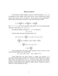
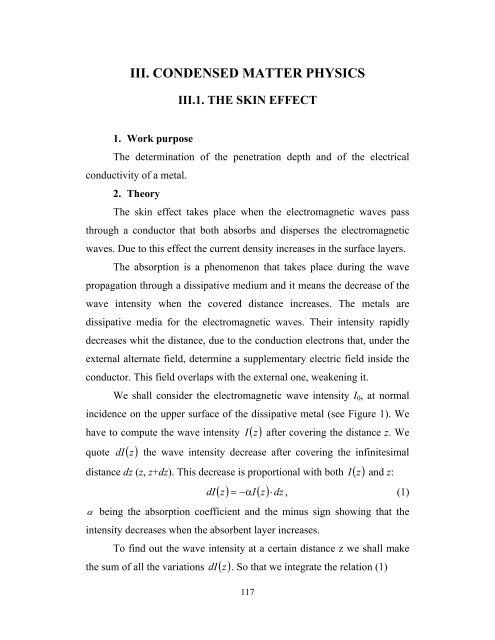
We shall consider the electromagnetic wave intensity I0, at normal
incidence on the upper surface of the dissipative metal (see Figure 1). We
have to compute the wave intensity I ( z)
after covering the distance z. We
quote dI ( z)
the wave intensity decrease after covering the infinitesimal
distance dz (z, z+dz). This decrease is proportional with both I ( z)
and z:
( z)
−αI
( z)
dz
dI = ⋅ , (1)
α being the absorption coefficient and the minus sign showing that the
intensity decreases when the absorbent layer increases.
To find out the wave intensity at a certain distance z we shall make
the sum of all the variations dI ( z)
. So that we integrate the relation (1)
117

and we obtain:
I
( z)
dI
∫ I
I
0
( z)
( z)
z
= −α
118
∫
0
dz
( z)
= I exp(
− z)
(2)
I 0 α . (3)
Figure 1.
The relation (3) shows that in a conductor the intensity of the
electromagnetic waves exponentially drops with the distance. As
the amplitude E ( z)
also drops exponentially with the distance:
where 0
2
I ∝ E ,
⎛ αz
⎞ ⎛ z ⎞
E ( z)
= E0
exp⎜− ⎟ = E0
exp⎜−
⎟ ,
⎝ 2 ⎠ ⎝ 2δ
⎠
(4)
E is the electric field amplitude of the incident wave and α = δ 1 ,
called penetration depth or skin thickness,, represents the distance over
which the wave intensity decreases e times. This depth depends on the
wave frequency ν and on the medium electric and magnetic properties.
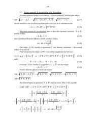
Let us consider an infinite conductor half-space. We choose a
Cartesian system of coordinate axes, such that the Ox and Oy axes belong
to the separation plane (z = 0), and the Oz axis is oriented towards the
interior of the conductor (see Figure 2). The electric field intensity vector
E r and the conduction current density vector j are oriented parallel to the

Ox axis, and the magnetic field induction vector B r is oriented parallel to
r
E = E , 0,
0
r
j = j , 0,
0
r
= 0 , B,
0 . The
the Oy axis. Hence ( ) , ( )
x
119
x
B y
and ( )
vector components are functions of the coordinate z and of the time t (these
components do not vary with the x and y coordinates). The equations that
govern the skin effect analysis are the equations of the electromagnetic
wave propagation in substances.
Figure 2.
Electromagnetic wave propagation through a conductor is studied by
taking into account that the conduction current density is much greater than
the displacement current density. Neglecting the displacement current, we
obtain the following equations for the electric and magnetic field
propagation through the conductors:
r
r ∂E
∆E
= σµ
,
∂t
r
r ∂B
∆B
= σµ
∂t
(5)
In our case, we have:
2
E x
2
x
2
y
∂
∂z
∂E
= σµ
∂t
∂ B y ∂B
, = σµ
. (6)
2
∂z
∂t
We remark that we may write the y component of the magnetic field B r as a
function of the x component of the electric field E r , if we use the Maxwell-
Faraday equation, which can be rewritten as follows:

( ∧ E)
∇ r
y
∂E
=
∂z
x
∂B
= −
∂t
120
y
. (7)
We accept a periodical time variation of the electric field, current density
and magnetic field such that:
( z,
t)
E(
z)
exp(
iωt
) , j ( z,
t)
= j(
z)
exp(
iωt
) , B ( z,
t)
= B(
z)
exp(
iωt
).
E x
x
y
= (8)
Replacing the expression of E x from Eq. (8) in Eq. (6), we obtain:
d
2
E
dz
( z)
2
= iωσµ
E
( z)
. (9)
Quoting p = iωσµ
2
, the differential equation (9) will become:
2
( z)
d E
2
dz
2
= p E(
z)
. (10)
The general solution of this differential equation is:
where A 1 and 2
( z)
= A ( pz)
+ A exp(
pz)
E 1 exp 2 − , (11)
A are two integration constants and
ωσµ
p = iωσµ
= i ωσµ = ( 1+
i)
, (12)
2
where we have used i ( 1+ i)
2
determined from the following conditions:
- for → +∞,
E(
z)
→ 0
z hence A 0 ;
= . The integration constants are
1 =
z → 0, E z = E 0 ≡ E = A .
- for ( ) ( ) 0 2
So, the solution (11) will become:
⎡
E(
z)
= E0
exp( pz)
= E0
exp⎢−
( 1+
i)
⎣
If we introduce the constant:
ωσµ ⎤
⋅ z⎥
.
2 ⎦
(13)
δ =
1
,
2ωσµ
(14)

the equation (13) may be written as:
⎡ z ⎤ ⎛ z ⎞ ⎛ z ⎞
E . (15)
( z)
= E0
exp
⎢
− ( 1+
i)
⎥
= E0
exp⎜−
⎟⋅
exp⎜−
i ⎟
⎣ 2δ⎦
⎝ 2δ
⎠ ⎝ 2δ
⎠
Taking into account the equation (8) and (15) we obtain then:
⎛ z ⎞ ⎡ ⎛ z ⎞⎤
E x . (16)
( z,
t)
= E0
exp⎜−
⎟exp⎢i⎜
ωt
− ⎟⎥
⎝ 2δ
⎠ ⎣ ⎝ 2δ
⎠⎦
To compute the current density j x and the magnetic field B y , we use
similar relations:
⎛ z ⎞ ⎡ ⎛ z ⎞⎤
j x ( z,
t)
= σE0
exp⎜−
⎟exp⎢i⎜
ωt
− ⎟⎥
, (17)
⎝ 2δ
⎠ ⎣ ⎝ 2δ
⎠⎦
2δσµ
⎛ z ⎞ ⎡ ⎛ z ⎞⎤
B y . (18)
In these relations,
( z,
t)
= E0
exp⎜−
⎟exp⎢i⎜
ωt
− ⎟
1+
i
⎥
⎝ 2δ
⎠ ⎣ ⎝ 2δ
⎠⎦
δ =
1
2ωσµ
121
=
1
4πυσµ
(19)
represents the penetration depth of the electromagnetic wave through the
conductor. Its value varies inversely proportional with the square root of
both the frequency of the field ν and the metal conductivity σ. Due to this
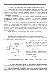
relation, we may notice that, simultaneously with the absorption, there is a
dispersion of the electromagnetic waves. If we increase the frequency ν, the
penetration depth decreases, meaning that the electromagnetic wave is
localized at the conductor surface. Due to this effect, the conductors used
for high frequency currents may look like pipes, to save up material.
In Table 1 we find the values of the penetration depth δ for an
alternate current through a copper conductor, for two frequencies of the
alternate current: 50 Hz and
decreases with the increase of the current frequency.
5
5 ⋅ 10 Hz. Hence the skin thickness δ

Table 1
Material σ (Ω -1 ·m -1 ) ν (Hz) δ (mm)
Copper 5.8 . 10 7 50 4.67
Copper 5.8 . 10 7 5 . 10 5 0.0467
In this paper we will determine the penetration depth δ and the
electrical conductivity σ for various frequency values. An electromagnetic
wave of a known frequency will fall on a conductor made from one or
more metallic plates and we will record the amplitude of the alternate
voltage determined in a receiving coil by the waves that pass through the
plates. Due to the proportionality between the voltage and the electric field
intensity, the amplitude of the incident alternate voltage U 0 drops
exponentially with the distance z and it is described by Eq. (4), meaning:
so that
or
⎛ z ⎞
U , (20)
( z)
= U 0 exp⎜−
⎟
⎝ 2δ
⎠
z
U = logU
− , (21)
2δ
log 0
U
log
U
0
122
z
= . (22)
2δ
If we draw the dependence of log U 0 U upon z, we will obtain a
straight line with the slope m = 1 2δ
. By determining the slope we will find
the penetration depth δ = 1 2m.
From the relation (14), we notice that δ is a linear function of 1 ν
δ =
1
⋅
4πσµ
1 1
= m ′ . (23)
ν ν

Drawing the dependence of δ upon 1 ν , and determining the slope
m’ of the straight line, we will compute the electrical conductivity:
where
µ ≈ µ
0
−7
= 4π ⋅10
N ⋅ A
3. Experimental set-up
-2
1
σ = , (24)
2
4πµ
m′
.
The experimental set-up (see Figure 3) is made of a sine oscillation
generator in the frequency range 10 – 100 kHz with a voltage level of 1000
mV (Versatester – type E0502), on which we connect an oscillator coil B1
and a receiving coil B2. Between them we put some metallic sheets (of Cu,
Al, Sn). By supplying an alternate current (through the coaxial cable C1) to
the B1 coil, a phenomenon of electromagnetic induction appears, inducing
an alternate voltage in the receiving coil B2. The induction current
frequency may be varied, and the induced voltage in B2 is measured with
the apparatus millivoltmeter (mV).
4. Working procedure
Figure 3.
1. The device is plugged in at 220 V a. c. and the coaxial cable C1 of the
oscillator coil B1 is connected at the muff “IESIRE 50”. We press the key
123

“10 – 100 kHz”, and the level selector (NIVEL INTERN) is on “1000
mV”.
2. With the fine frequency selector “FRECVENTA” we choose a frequency
(for instance 50 kHz), which is read on the digital display, by choosing
“INTERN F” from the internal switch.
3. We determine on the voltmeter the voltage U0 for zero absorber
thickness, switching the external switch on “EXTERN F”.
4. We choose a metallic sheet of a known thickness z (zAl = 80 µm, zCu = 40
µm, zSn = 50 µm), which is placed between the coils B1 and B2, and we
determine the received voltage on the millivoltmeter, switching the external
switch on “EXTERN F”. We successively add sheets of the same metal and
we record for every total thickness z’ = n·z (n being the total number of
sheets), the received voltage. At least another 4 values of the frequency (for
instance ν = 60, 70, 80, and 90 kHz) must be used for all thicknesses. The
obtained data will be filled in Table 2:
Table 2
Metal ν (kHz) z (mm) U (mV) U0/U log U0/U δ (mm)
... ... ... ... ... ... ...
5. We shall repeat the experiment for the other metals too. For each metal,
we will fill the obtained data in Table 2.
6. In order to find the electrical conductivity σ of the used materials, after
data processing, Table 3 is filled in:
Table 3
Metal ν (kHz) ν 1/2 (kHz 1/2 ) δ (mm)
... ... ... ...
5. Experimental data processing.
1. For each metal and fixed frequency ν1, ν2, ..., we draw on the same
log U U = f z , where U0 is the voltage when
diagram the dependency ( )
0
124

all metallic sheets are removed. Using the relation (22) we obtain, for each
metal, a family of straight lines for which we will determine their slopes
m1, m2, ... We compute the penetration depths δ1, δ2, ..., knowing that
δ = 1 2m
.
2. Using the data from Table 3, another graph is drawn, with the
dependency of δ upon 1 ν . A straight line of slope m’ is obtained for
each metal and using the relation (24) the electrical conductivities σ are
determined.
3. In order to determine the slope of the line y = ax , we can apply the least
square method. Then, the estimated value for the slope is:
n ⎛ n ⎞⎛
n ⎞
n∑
x ⎜ ⎟⎜
⎟
i yi
−
⎜∑
xi
⎟⎜∑
yi
⎟
i=
1 ⎝ i=
1 ⎠⎝
i=
1 ⎠
a =
, (25)
n
2
2 ⎛ n ⎞
n∑
x − ⎜ ⎟
i ⎜∑
xi
⎟
i=
1 ⎝ i=
1 ⎠
where n is the number of pairs {xi, yi} experimentally measured. The value
of the parameter a is affected by the mean square deviation:
⎧
⎫
⎪ n
2 ⎪
⎪ ∑ ( yi
− axi
) ⎪
⎪ i=
1
⎪
s a = ⎨
⎬
2
⎪ ⎡ n
⎤ ⎪
2 ⎛ n ⎞
⎪(
n −1)
⎢n∑
x − ⎜ ⎟ ⎥
i
⎪
⎪ ⎢ ⎜∑
xi
⎟
1 1 ⎥ ⎪
⎩ ⎣ i=
⎝ i=
⎠ ⎦ ⎭
. (26)
4. The linear dependence between log U 0 U and z is given by the relation
logU 0 U = z 2δ
. We quote y = logU
0 U , x = z , a = 1 2δ.
The
unknown a must be expressed as a function of its estimated value and mean
square deviation
a = a ± sa
. (27)
Similarly
δ = δ ± s δ .
δ = δ a , we have:
(28)
Taking into account the relation ( )
2 ⎛ dδ
⎞ 2
s = ⎜ ⎟ s
δ
a .
⎝ da ⎠a=
a
(29)
5. We apply the same method for the determination of the conductivity σ.
In this case y = δ , x = 1 ν and
σ = σ ± s . (30)
125
2
σ
1 2