Incorporating Uncertainty into Discounted Cash Flow Equity ...

Incorporating Uncertainty into Discounted Cash Flow EquityValuationsJon ComeauEconomics Senior ProjectFall 2009Advisor: Dr. Eduardo Zambrano[Abstract]: The discounted cash flow valuation is widely used by corporations, financialadvisers, and investors to help guide investment decisions. However, the valuation estimatescontain a high level of uncertainty. Multiple academics and practitioners have developed waysto combat uncertainty in investment decisions. This paper is aimed at giving decision makersmore information to help improve the decision making process via Monte Carlo simulations andutility theory.1

Table of ContentsI. Introduction ............................................................................................................................................... 3II. Literature Review ..................................................................................................................................... 5III. DCF Model 1: Overview ........................................................................................................................ 10DCF Method ........................................................................................................................................ 10WACC .................................................................................................................................................. 11IV. DCF Model 1: Data and Analysis ........................................................................................................... 13V. DCF Model 2: Overview ......................................................................................................................... 17Incorporating Probability Models ....................................................................................................... 18Expected Utility and Certainty Equivalents ........................................................................................ 20VI. DCF Model 2: Data and Analysis ........................................................................................................... 23DCF Valuation...................................................................................................................................... 23Expected Utility and Certainty Equivalents ........................................................................................ 25VII. Conclusion ........................................................................................................................................... 27References ................................................................................................................................................. 30Appendix A: Model 1 ................................................................................................................................. 32Appendix B: Model 2 .................................................................................................................................. 402

I. IntroductionDiscounted cash flow (DCF) analysis is a method of valuing investments including equity, realestate, corporate projects and even entire companies. The method essentially estimates future cashflows and discounts them using an appropriate rate to determine an estimate of their present value.The concept of DCF is derived from the fact that the value of an investment today should be equal to thepresent value of the cash flow it will generate. Discounting the cash flows is necessary to account formoney being received at a future date being worth less than money received today because it could bereinvested to earn additional income. The method was first developed by Arthur M. Wellington, arailroad engineer, in the late 19 th century. The method was further developed by academics andengineers post World War Two. DCF valuations are now widely used by firms to make irrevocable capitalbudgeting decisions (Dulman).Beyond capital budgeting decisions, DCF valuations can be used to determine enterprise value,the estimated value of an entire company, and the intrinsic value of a firm’s equity. Value investors usevaluations, including DCF, to find stocks that are trading at a significantly different price than theirestimated intrinsic value (“Value Investing”). To calculate a firm’s intrinsic equity value using the DCFmethod future free cash flow (FCF) must be estimated. To obtain the FCF estimate the firm’s incomestatement and balance sheet is forecasted out for typically 5 years. Beyond the 5 year period theGordon Growth Model is used to calculate a terminal value which is the value of the FCF a firm willgenerate into infinity calculated as perpetuity. The company’s weighted average cost of capital (WACC)is then used as the discount rate to determine the present value (PV) of FCF. To determine equity value,the current level of the firm’s debt is subtracted from PV of FCF, which gives the cash flow available to3

equity investors. That value is then divided by the current number of shares outstanding to obtain theintrinsic value of the company’s stock price (Gorman).Due to the calculated intrinsic values being based on forecasts, the resulting estimate isuncertain. The only input in the DCF calculation that is not a forecast is the WACC used to discount thecash flows. However, the values used for the exogenous variables in the equation can differ frompractitioner to practitioner. The uncertainty inherent in DCF calculations has significant real worldimplications. Firms make large and often irrevocable investment decisions based on DCF valuations.According to a survey of 37 leading Fortune 500 firms, 96% of corporations and 100% of financialadvisers surveyed use the DCF technique to evaluate investment opportunities (Bruner 190). Valueinvestors who utilize the DCF method are essentially betting that their valuation is accurate, and thefirm’s intrinsic value will be realized in the market during a particular time horizon. Despite the highlevel of uncertainty and the dependence on assumptions, DCF estimates are ubiquitous in the world offinance. Cal Poly Finance Professor John Dobson summarized this point by relating to his students thatwhen all you have is a hammer everything looks like a nail, and in finance the hammer is the DCFvaluation.The objective of this paper is to analyze ways for value investors to make more informedinvestment decisions under uncertainty. Specifically, the paper focuses on incorporating probabilitymodels into a DCF equity valuation and running thousands of Monte Carlo simulations to derive anexpected equity value rather than a single point estimate. The descriptive statistics that can becalculated from the simulation outputs should help illustrate the level of uncertainty in the valuationand help with the decision making process. The paper then looks at how calculating the expected utilityof the investment based on a fixed level of risk tolerance can be used as an added decision making4

criteria. The decision maker can compare the expected utility of the investment to the expected utilityof alternative investments or of not investing at all and choose the investment that maximizes expectedutility. Running Monte Carlo simulations and calculating expected utility will not necessarily equate tomore profitable investment decisions. The real benefit of applying these methods is framing theinvestment decision in the context of the level of uncertainty surrounding the estimate and the decisionmaker’s risk profile.The paper begins by over viewing previous work regarding investment under uncertainty, andalthough there is an extensive amount of literature on the subject only a few studies closely related tothis paper will be profiled. The paper then overviews a DCF equity valuation of Cracker Barrel (Nasdaq:CBRL) conducted in December 2008. The DCF valuation is then redone by incorporating uncertainty intothe FCF forecasts and running 5,000 simulations. Finally, the paper looks at calculating the expectedutility of the investment by using a constant level of risk tolerance.II. Literature ReviewVarious Academics have analyzed ways to incorporate uncertainty into investment decisions.Beginning in the 1930’s Benjamin Graham laid the foundation for the modern value investor in SecuritiesAnalysis and The Intelligent Investor. In both books, Graham made a clear distinction between investingand speculating and argued that intelligent investors can protect themselves from the risk of uncertaintyby making investments with a particular margin of safety. Graham made the distinction betweeninvestment and speculation in Securities Analysis as follows: “An investment operation is one in which,upon thorough analysis, promises safety of principal and a satisfactory return. Operations not meetingthese requirements are speculative” (3). Graham advocates against investors timing the market,5

selecting stocks thought to outperform the market in the short term, and selecting stocks thought tooutperform the market in the long term (i.e. growth stocks). The problem with those strategies is thedifficulty of accurately predicting the future and doing it better than a “host of competitors” (11).Graham promotes investing in securities at bargain levels relative to their fundamental valuesand in other promising securities and leading investment funds when the market is not too high (16). Hebelieves these opportunities generally occur when the market is at depressed levels and when individualissues are particularly unpopular (173). The margin of safety advised by Graham is essentially pickingsecurities whose value to the investor does not depend on accurately predicting the future. The marginof safety for fixed income investments can be thought of as the difference between the value of thecompany and their level of debt. For example, if a company is worth $30 million and they have $10million in debt the company could shrink by 2/3 before there is any risk to the debt holders. For ordinarycommon stock Graham describes the margin of safety as the difference between the expected earningpower of the stock and the going rate for bonds. To mitigate the uncertainty risk that is inherent ininvestments, Graham promotes investing in securities that have strong fundamentals at bargain levelsthat have an adequate margin of safety (256). The difference between the intrinsic or fundamentalvalue and the low level the security is trading at provides a cushion against miscalculations and adversemarket conditions.When making investment decisions the worth of not investing immediately is another factorthat can be taken into consideration. In Investment Under Uncertainty Avinash Dixit and Robert Pindyckargue that the value of delaying the investment should be incorporated into the decision makingprocess. One technique is to view the investment decision as a real option. Firm’s make large oftenirrevocable investment decisions continuously throughout time. The irreversibility of investment6

decisions requires that the standard NPV analysis taught in business schools be adjusted. TraditionalNPV analysis ignores the opportunity cost of investing now. If the investment can be made now or at afuture date and if it is irrevocable then the decision to invest can be viewed and valued as a call option(26). The adjusted NPV method developed in Investment Under Uncertainty can be utilized by valueinvestors via incorporating the value of the option into the DCF.Kenton Yee’s Deep-Value Investing, Fundamental Risks, and the Margin of Safety, in the Journalof Investing, applies the option framework to Benjamin Graham’s margin of safety. Yee views the marginof safety as the discount (the intrinsic value minus the market value) that is equal to the value of theoption to delay the investment. The paper develops a model to determine how large a margin of safetya value oriented investor should demand. Value investing relies on mispricing, a convergence datewhere the intrinsic value will be realized in the market, and the ability to establish the desired positionbefore the convergence date. Yee identifies four risks to value investors:1. Market risk: volatility of the market price2. News risk: news that will disrupt the investors intrinsic value estimate3. Valuation risk: The intrinsic value estimate may be systematically biased or imprecise4. Convergence risk: uncertainty about when the market price will converge to theestimated valueYee incorporates those risk factors into calculating appropriate margins of safety using the real optionsframework. Analyzing companies in the S&P 500, Yee calculates the typical margin of safety to bebetween 20-30% of share prices. Like Graham, Yee advocates making investments with a large marginof safety to increase the probability of a desirable outcome.7

Nick French and Laura Gabrielli analyze ways to incorporate uncertainty into the DCF method ofvaluing real estate in their Discounted cash flow: accounting for uncertainty study. The authors’ find thatalthough DCF real estate valuations are uncertain they are generally reported as a single point estimatewithout any reference to the uncertainty behind it. A point estimate is a common approach that usesthe valuer’s best estimate of the unknown value to make the calculation without any consideration ofuncertainty (Myerson 49). The cash flows from real estate investments are uncertain which results inthe valuation being uncertain. The projected cash flows are based on the best estimate of aprofessional. The authors argue that probabilities should be incorporated into those estimates. Normaldistributions are the most statistically robust, but the Triangular distribution better reflects thejudgment and thought process of the valuer. The valuer can use market information to determine themost likely outcome and then asses what they believe to be the best and worst outcome. The study usesCrystal Ball, a software package, to run Monet Carlo simulations. Instead of producing a single pointestimate the simulation carries out multiple iterative calculations using random values that are based onthe provided triangular distribution values. The process is repeated thousands of times and the mean ofthe resulting valuations is used as an expected estimate rather than a single point estimate. The studyfound that the expected value is not significantly different than the point estimate, but incorporatinguncertainty adds beneficial information about the uncertainty of the result. One benefit is thesimulation results provide a standard deviation which describes the risk of the valuation estimate notbeing realized. A range can be provided to show the probability of the value falling between a certaindollar range. Incorporating uncertainty places the valuation estimate in the context of the uncertainty ofinputs and the risk of the output estimate not being realized (French).8

Another method of making investment decisions under uncertainty is by looking at the expectedutility of the investment. In Probability Models for Economic Decision Making Dr. Roger Myersonoverviews how utility can be incorporated into investment decisions. The investor’s risk tolerance can beestimated using a hypothetical binary lottery with each pay off being equally likely. If the risk tolerancecan be assumed to remain constant then the investor’s utility from various gambles can be computed.Using Monte Carlo simulations similar to the study mentioned above, the expected utility of aninvestment can be found by taking the average of thousands of simulation results. This value can thenbe compared to the expected utility of other investments or the utility of not investing at all. Thismethod allows decision makers to make choices based on utility maximization given a specific riskprofile.Graham and Yee’s objective in dealing with investment under uncertainty is to increase theprobability that the investor will experience favorable results. As opposed to wealth maximization,French and Myerson focus on increasing the information available to decision makers. The focus of thispaper will not be on increasing the chances of wealth maximization but rather on increasing informationto aid in the decision making process. The Monte Carlo simulations will not necessarily provide a moreaccurate estimate, but it will illustrate the uncertainty surrounding the estimated stock price. UnlikeFrench and Gabrielli’s study, this paper will use the Generalized Log-Normal distribution rather than theTriangular distribution to incorporate uncertainty into the forecasts. The Triangular distribution providesa smaller range of possible randomly generated forecasts, and the Generalized-Log normal is used in thispaper to reflect my higher level of uncertainty regarding CBRL’s FCF forecasts. Incorporating theexpected utility will add another decision making criteria to the margin of safety concept that is widelyused by value oriented investors.9

III. DCF Model 1: OverviewDCF MethodThe discounted cash flows or free cash flow for the firm (FCFF) is the method used in this studyto calculate the intrinsic value of CBRL’s equity. The FCFF is the after tax earnings adjusted fordepreciation, changes in working capital, and increases in capital expenditures. The method ofcalculating the overall cash flow to a zero debt firm used in this paper is listed below:FCFF = EBIT (1-t c ) + (Depreciation + Amortization) – Cash Flows from Capital Spending – Cash Flows fromChanges in Working CapitalwhereEBIT = Total Revenue – Cost of Goods Sold (COGS) – Sales, General & Administrative Expenses (SG&A) –Other Indirect Expenses – Depreciation & AmortizationCash Flows from Capital Spending = Purchases of Property Plant & Equipment (PPE) - Sale ofPPE before Taxes + Taxes on Sale of PPECash Flows from Changes in Working Capital = Increase (Decrease) in Accounts Receivable +Increase (Decrease) in Inventory + Decrease (Increase) in Accounts Payable10

The DCF discounts the year by year FCF and a terminal value, V n , which is calculating using the GordonGrowth Model. The discount rate used is the firm’s weighted average cost of capital (Bodie 613).Enterprise Value = ∑ + , where V n = To obtain the intrinsic value of equity, the current value of CBRL’s debt is subtracted from theenterprise value, and a share price is obtained by dividing the value available to equity investors by thecurrent number of shares outstanding.Weighted Average Cost of CapitalWACC is the dominant discount rate used in DCF analyses (Bruner 173). It is given as follows:whereWACC = (W debt (1 - t c )K debt )+(W preferred K preferred )+(W equity K equity )K = component cost of capitalW= weight of each component as % of total capitalt c = marginal corporate tax rateThe cost of equity can be calculated via the capital asset pricing model (CAPM) or a multifactormodel. This valuation ran market model regressions to determine the cost of equity using both the11

CAPM and a multifactor model. The CAPM was developed in 1964 by William Sharpe, John Linter, andJan Mossin as method of calculating the required return of an asset (Bodie 279). The equation isK e = R rf + β(R m – R rf )whereR rf = Interest rate available on a risk free bondR m = Return required to attract investors to hold the broad market portfolio of risky assetsR m – R rf = The equity risk premiumβ = The relative risk of the particular asset (Bruner 175)Another approach to calculating the cost of equity is using a multifactor model which aims toidentify macroeconomic sources of systematic risk (i.e. risk that should be rewarded and thus increasethe required return on an asset) (Bodie 424). This valuation incorporates the Fama French three factormodel. The equation is given below:K e - R rf = α 0 + β 1 E[R(Market-rf)] + β 2 E[R(SMB)] + β 3 E[R(HML)]whererf = Interest rate available on a risk free bondE[R(Market-rf)] = The expected return on the market minus the Interest rate available on a riskfree bondE[R(SMB)] = The expected returns of small market cap stocks over big market cap stocksE[R(HML)] = The expected returns of high book/market value stocks over low book/marketstocks12

The firm specific factors are incorporated into calculating the expected return on a security due to longstanding empirical observations that firm size and the book-to-market ratio predict stock returns thatare inconsistent with the CAPM (Bodie 336). There is much debate over the validity of the CAPM andmulti factor models, but for the purpose of this paper it will be assumed that both adequately predictreturns. The model that results in the highest statistical significance is used in this valuation.The DCF model contains multiple assumptions beyond the forecasted FCF. The WACC value usedcan vary dramatically and will have a significant impact on the calculated value. A study examining theWACC estimation practices of various corporations, financial advisors, and finance textbooks foundsignificant deviations in the practices of calculating WACC (Bruner 171). To account for the variouspossible values of the WACC a sensitivity analysis is incorporated into the second valuation. Theobjective of this paper is not to analyze the best practices of DCF valuations. The paper assumes themethods of calculating the DCF valuation in this study is valid and will focus on adding information tothe decision making process.IV. DCF Model 1: Data and AnalysisFCF Forecasts:To forecast CBRL’s FCF, 10 years of financial data were obtained from MergentOnline.Specifically, balance sheet, income statement, and statement of cash flows data from 1999-2008 areused. To estimate FCF revenue must first be forecasted (Figure 1 of Appendix A). Multiple regressionswere run to try and determine factors that explain changes in CBRL’s sales. However, due to the lack of13

an adequate model, revenue forecasts for 2009-2011 from Capital IQ and 2012-2013 forecasts fromValue Line are used (Figures 2 and 3 of Appendix A). COGS, SG&A, and other indirect expenses areestimated using a 10 year historical mean percentage of sales. Depreciation and amortization isestimated using Value Line’s future estimate. 2009 and 2010 purchases of PP&E are determined by usingestimates listed on Cracker Barrel’s 10-K. The remaining PP&E values use a 15 year historical average.The 2009 estimate of gains from the sale of PP&E is taken from the company’s 10-K and the remainingyears are forecasted from a 15 year historical average. Changes in working capital are estimated byusing a 10 year historical average of days A/R, days inventory, and days A/P. Cracker Barrel predicted a35% corporate tax rate for 2009, and that value is used for the 2009-2013 forecasts. The forecasting isdone in Excel, and all the values mentioned above are located in a driver box that is used to computethe forecasted values (Figure 4 of Appendix A). With those values forecasted, the FCF generated from2009-2013 is calculated (Figure 5 Appendix A).Terminal Growth Rate:To calculate the value of Cracker Barrel beyond 2013 a terminal growth must be determined.The terminal growth rate is highly subjective and can essentially be a shot in the dark. Investment Bank’susing the Gordon Growth Model to calculate enterprise values will typically use the country’s GDPgrowth rate, the rate of inflation, or something similarly conservative (“Breaking into Wall Street”). Therate used in the calculation is 3%, and is determined by taking the 1989-2009 average annual growthrate of the U.S.’s GDP from the Bureau of Economic Analysis.14

WACC:To properly determine the present value of the company’s future cash flows it is necessary todiscount those cash flows at the company’s cost of capital. To determine the weighted average cost ofcapital for CBRL, I first determined the expected return of their equity to be 10.43% via the Fama Frenchthree factor model.Cost of Equity/Market Model Regressions:To determine the company’s cost of equity market model regressions are run using both thecapital asset pricing model (CAPM) and the Fama French three factor model. For the CAPM regression,60 months of stock price data from November 2003 to October 2008 from Yahoo! Finance is used. TheS&P 500 is used to represent the market, and to compute accurate returns S&P 500 dividends estimatedby Yale University professor Robert Schiller are factored in. To get the excess returns, the returns on 1year U.S. Treasury-notes obtained from economagic.com are subtracted from the returns of bothCracker Barrel and the S&P 500. To make the data accurate the T-note returns are divided by 1200 toget them in monthly decimal format. The regression resulted in an adjusted R 2 of .1079033 and a β 1 of.79691. β 1 is not statistically different from 1, meaning CBRL approximately moves with the market. Thefollowing model was run using OLS:R(CBRL) = β 0 + β 1 *R(Market-rf) + εLike the CAPM, 60 months of stock price data from November 2003 to October 2008 fromYahoo! Finance is used for the Fama French regression. In addition, 60 months of data from November15

2003 to October 2008 was taken off of Ken French’s website. The data includes excess market returns,returns of high book/market value stocks over low book/market stocks, and returns of small market capstocks over big market cap stocks. The following regression model was run using OLS:R(CBRL) = β 0 + β 1 *R(Market-rf) + β 2 *R(SMB) + β 3 *R(HML) + εThe HML estimator is not statistically significant. The variable was removed and a restricted Ftest shows the restriction is valid. The restricted model results in statistically significant estimators withβ 1 = .73982 and β 2 =.93548. The restricted model has an adjusted R 2 of .165766. The Fama French modelis used to calculate the cost of equity due to it having a higher adjusted R 2 (Figure 6 Appendix A).For this valuation the betas were manually calculated. However, a majority of corporations andfinancial advisors will use betas from published sources (Bruner 191).Cost of Debt:At the time of the valuation Cracker Barrel’s S&P credit rating was BB- (“CBRL Group IncNasdaqGS CBRL Fixed Income”). As of fiscal 2008, Cracker Barrel had $789.9 million in debt. 99.5% ofthe company’s debt was in term loans and the rest in capital leases and short term revolving lines ofcredit (“CBRL Group Inc NasdaqGS CBRL Financials”). Since Cracker Barrel has no outstanding bonds, ayield to maturity is calculated by using an outstanding bond, found on Yahoo! Finance, within a similarindustry and with a similar maturity date. The cost of debt is calculated to be 8.306%.16

Weights:Best practices in calculating the WACC dictates using the market values of debt and equity tocalculate the weights (Bruner 175). The market value of equity of $405,074,770 at the date of thevaluation is calculated by multiplying the current share price of $17.78 by the number of sharesoutstanding. The value of debt was taken from figures provided by Capital IQ.CBRL’s current tax rate of 30.2% is used. Cracker Barrel had no preferred shares, so that elementof the equation dropped out to zero. CBRL’s WACC is calculated to be 7.34% (Figure 7 Appendix A).Estimated Value of CBRL’s EquityThis valuation of CBRL determines the present value of CBRL’s assets in 2008 to beapproximately $2.2 billion. Subtracting off the approximately $1.2 billion in liabilities leaves $967,890available to equity investors. Dividing the $9.7 million PV of equity results in an intrinsic share pricevalue of $42.44 (Figure 8 Appendix A). With CBRL trading at $17.78/share at the time of the valuationthis represents a significant undervaluation of the company’s equity and this analysis resulted in atheoretical buy decision.V. DCF Model 2: OverviewThe original model was redone by incorporating probability models and running thousands ofMonte Carlo simulations. Like the previous model, this valuation is done for CBRL as of their fiscal year17

ending in 2008. The simulation output is used to calculate the expected stock price and descriptivestatistics, as well as the expected utility of the investment.Incorporating Probability Models:The forecasted values used to compute the future FCF in model 1 are single point estimateswhich results in the estimated stock price being a single point estimate. To combat this, probabilities canbe incorporated into the forecasts. This model uses the Generalized-Lognormal distribution. Thedistribution is meant to represent my uncertainty regarding the true value of the forecasts and is notassumed to accurately represent the true distribution of the variables. The Generalized-Lognormaldistribution is defined by three quartile boundary points: Q 1 , Q 2 , and Q 3 .The quartile points characterizethe distribution by specifying the .25, .50, and .75 cumulative probabilities. Q 1 , Q 2 , and Q 3 are thequartile boundary points for a Generalized-Lognormal distribution when for an unknown value XP(X < Q 1 ) = .25, P(X < Q 2 ) = .50, and P(X < Q 3 ) = .75If X is a continuous random variable then the actual value of X is equally likely (i.e. probability of ¼) to belocated in any of the 4 quartiles. Q 2 can also be defined as the median value of the distribution (Myerson122).To estimate the FCF forecasts subjective probability assessments are used. Rather than to thinkin sophisticated statistical concepts it can be easier to think in terms of a simple binary lottery. Theperson conducting the assessment can think of a simple lottery that pays either $1000 or $0 with eachof the outcomes being equally likely. For example, the subjectively assessed Q 2 would be the point18

where the person would be indifferent between the following 2 lotteries: (1) pays $1000 if the truevalue, N, is < Q 2 and $0 otherwise and (2) pays $1000 if N ≥ Q 2 and $0 otherwise (Myerson 127). Thesubjective probabilities would be defined asP(N < Q 2 ) = P(N ≥ Q 2 ) = ½The process is continued until the 3 quartile boundary points are defined such thatP(N < Q 1 ) = .25, P(N < Q 2 ) = .50, an P(N < Q 3 ) = .75The simulation is run in Excel using the Simtools add-in developed by University of ChicagoProfessor Roger Myerson. Like the previous model, this valuation is done in Excel. However, the driversin this model are random variables generated by the subjectively assed quartile boundary points. Theadd-in utilizes Excel’s RAND() function which generates a number between 0 and 1 with each valuebeing equally likely. The RAND() function is used as the probability input in the Generalzied-lognormalequation used to incorporate probabilities into the forecasts. The Excel function used is= GENLINV(RAND(), Q 1 , Q 2 , Q 3 )Minimum and maximum values can be included in the function by including a low and high value afterthe quartile boundary points (Myerson 124).= GENLINV(RAND(), Q 1 ,Q 2 ,Q 3 ,L,H)19

The drivers from the original model are used as the median values for the probabilitydistributions, since they are essentially my best estimate. The future FCF generated from 2009-2013 iscalculated from the randomly generated drivers. Then 5,000 simulations are run on the estimatedintrinsic stock price. From the simulation output an expected stock price is calculated, as well as otherdescriptive statistics.The purpose of using the probability models based on the Generalized-Lognormal distribution isnot to necessarily obtain a more accurate stock price. Using probability models does not remove thedanger of the valuation being based on bad assumptions. In fact, this valuation uses my own subjectiveassumptions, as well as assumptions from Capital IQ and Value Line. All simulation models face theproblem of garbage in garbage out; meaning the accuracy of the simulation is dependent on thespecified parameters. The real benefit from running the simulation comes from the descriptive statisticsthat can clearly illustrate the level of uncertainty in the valuation.Expected Utility and Certainty Equivalent:To improve the decision making process this valuation also includes the expected utility of theinvestment. The expected utility (E(U)) can be compared to that of a similar investment or of notinvesting at all. The E(U) in this paper is calculated by computing my own risk tolerance. Most investor’shave at least a general sense of the risk they are willing to take. A risk seeking investor may prefer younggrowth companies that have no demonstrated ability to generate predictable earnings, while a highlyrisk adverse investor may prefer to older companies with predictable earnings that pay a stabledividend.20

To specifically define an individual’s risk tolerance a simple binary lottery can be used todetermine a certainty equivalent (CE). For a simple lottery, the CE would be the lowest possible amountof money an individual would be willing to accept instead of taking the gamble. If an individual wasoffered a gamble that paid $5000 or $0 with each having a probability of 0.5 then the expectedmonetary value (EMV) of the gamble is 0.5*($5000 + $0) = $2,500. A perfectly risk neutral individualwould have a CE equal to the EMV. If the individual is risk adverse then they would have a CE that isbelow the EMV. The difference between the EMV and the CE is known as the risk premium (RP).Specifically,RP = EMV – CEWhen looking at multiple gambles the one with the highest CE should be chosen because it is worth themost (Myerson 83).Utility theory provides a useful way to analyze CEs while incorporating the decision maker’swillingness to take risks. Utility theory assumes that individuals have personal utility functions withspecific utility levels for every possible monetary level, and that individuals will always want to maximizetheir expected utility. With the choice of 2 gambles that have a random payoff of X for gamble 1 and Yfor gamble 2, a risk neutral individual will prefer 1 if E(X) > E(Y). However, according to utility theory, thefirst gamble will be preferred when E(U(X)) > E(U(Y)), where U = Utility. The CE for gamble 1 should havethe same utility as the expected utility of the gamble. The basic equation isU(CE) = E(U(X))21

Von Neumann and Morgenstern argued in 1947 that rational decision makers should makedecisions involving risky gambles based on utility theory. Accurately assessing an individual’s utilityfunction is difficult, but in this case it is made easier by assuming a constant level of risk tolerance.Assuming that an individual’s risk tolerance remains constant means that if the payoff of a gamblechanges by a fixed amount in all possible outcomes of the gamble then the CE of the gamble will changeby the same amount. Constant risk tolerance allows independent gambles to be analyzed separately(Myerson 84). With constant risk tolerance the utility function can be defined asU(x) = -e (-x/r)where r is the risk-tolerance constant. The Simtools add-in used in this valuation has a UTIL function thatis used in place of the above function (UTIL (x,r) = -e (-x/r) ). The benefit of assuming constant risk toleranceis that only the parameter, r, needs to be calculated to determine the utility from different payoffs.The parameter, r, can be calculated by a subjective assessment. The decision maker can think ofa gamble that is similar to the potential real life payoffs. The gamble should have a high and low payoffwith each being equally likely. The decision maker can then assess their CE. With the high and lowpayoffs denoted by H and L, the expected utility function isE(U) = 0.5*-e (-H/r) + 0.5*-e (-L/r)The utility of the decision maker’s CE must equal the expected utility of the gamble, thus r can be solvedby setting the 2 equations equal to each other.22

0.5*-e (-H/r) + 0.5*-e (-L/r) = -e (-CE/r)This study uses the Simtools add-in that solves for r given a high and low payoff and a CE. Thegeneral equation used in Excel is RISKTOL = (H, L, CE). With a defined constant risk tolerance parameterthe expected utility and certainty equivalent can now be calculated for any simulated gamble orinvestment (Myerson 85-86).This study assumes that on December 2, 2008, I purchased 100 shares of CBRL at the price of$17.78. Then from the simulation data my wealth a time T is calculated, with T being equal to the lengthof time it takes for the intrinsic stock price to be realized in the market. For the utility analysis, it isassumed that the intrinsic value and market value will converge at some date T. The initial investment of$1778 ($17.78/share *100 shares) is subtracted from the new value of the investment at date T tocalculate the profit from each simulation result. For the ease of computation and the ambiguity of dateT, the time value of money is ignored in computing profits as is bid ask spreads and other transactioncosts. Then from each simulated payoff my utility is calculated based on my subjectively assed r. Fromthese figures the E(U), EMV, and risk premium is calculated. The E(U) of the investment is compared tomy utility of not investing. Assuming my risk tolerance profile remains constant, I can determinewhether investing or not investing will maximize my utility.VI. DCF Model 2: Data and AnalysesDCF:This valuation used the same 10 year financial data from MergentOnline. To perform thesubjective probability assessment for the quartile boundary points I used the point estimates from the23

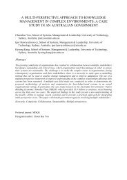
original model as a guide. Specifically, the point estimates used to estimate the future financialperformance were used as the median quartile values. To help guide my decision making process the 1and 99 percentile values are calculated (Figure 1 Appendix B). I could assess whether I believed the valuebeing analyzed had a 1% chance of being above or below a certain value.The WACC for the new model is held constant at the same 7.37% value used in the originalmodel. However, a sensitivity analysis was performed using the original model. Both models are highlysensitive to the discount rate used. Decreasing the WACC by 37 basis points (i.e. 0.37%) to 7% increasesthe stock price by 17%, while increasing the discount rate by 63 basis points to 8% decreases the stockprice by 28% (Figure 5 Appendix B).The expected stock price was calculated by taking an average of the 5,000 simulated prices. Thenewly estimated price is $67.07 vs. the $42.44 originally calculated. This represents a 58% increase inthe estimated intrinsic value. Nick French and Laura Gabrielli’s study on incorporating probabilitymodels into real estate DCF valuations only found a 10% difference between the point estimate and theexpected value they calculated. This discrepancy is likely due to me having a larger amount ofuncertainty regarding the true values of the forecasts. Also, the Triangular distribution used in theirstudy provides a smaller range of possible randomly generated forecasts. The difference in the level ofuncertainty is reflected in the different standard deviations of both valuations. The standard deviation intheir study is £9,068 with a mean of £203,662 and a median of £202,489. My study has a standarddeviation of $2,478 with a mean of $67.07 and a median of $47.16 (Figure 2 Appendix B). Experiencedpractitioners will likely be able to build simulations with smaller levels of uncertainty resulting in thepoint estimate being closer to the average of the simulated values. However, it is important to keep inmind that even if the practitioner is confident in their estimates and incorporates highly efficientdistributions it does not necessarily mean that future events will match their predicted distributions.24

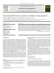
With an alpha of 10% the confidence interval for the expected stock price is ($9.25; $124.88).The calculation is as follows:µ ± 1.65*(σ/√)Lower bound = $67.07 – 1.65 *($2,478/5000 1/2 ) = $9.25Upper bound = $67.07 + 1.65*($2,478/5000 1/2 ) = $124.88Assuming I invested in 100 shares at December 2, 2008 at the price of $17.78, the valuation predictswith 90% certainty that my wealth at date T would be between -$852.51 and $10,710.22, ignoringtransaction costs and the time value of money.The range computed from this valuation is significantly different than the estimate provided byValue Line. Projections for CBRL’s stock price provided by Value Line are between a high and low valueof $65-$45 for 2011-2013. The expected value is only 3% higher than Value Line’s high estimate, butthere is a drastically higher level of uncertainty regarding the range of possible stock prices (Figure 6Appendix B). Again, this could be caused by my own inexperience causing higher levels of uncertainty.Also, Value Line does not state the method of calculating their projections or the level of confidence fortheir predicted stock price values. With an alpha of 50% the interval of CBRL’s expected stock pricedecreases to ($44.64; $89.49). Based solely on the expected stock price this valuation would also lead toa theoretical buy decision. However, taking into account the standard deviation and confidence interval25

of the estimate the decision to invest is no longer a clear yes. The following section of the paper focuseson calculating the expected utility to help make the investment decision.Expected Utility and Certainty Equivalent:To calculate my risk tolerance constant I looked at a hypothetical gamble that had a 50% chanceof paying $5000 or a 50% chance of paying $1000. The EMV of this gamble is $3000. The high and lowvalues are chosen to reflect possible pay offs of the CBRL investment. Although the simulation indicatesa potential loss, I am assuming there is a reasonable chance of two equally likely profitable outcomes.The high and low payoffs represent a stock price of approximately $67 and $28, respectively. Thehypothetical gamble is not meant to be a 100% accurate representation of equally likely outcomes frominvesting CBRL, but rather it is meant to be a proxy for a potential payoff. Given the depressed level ofthe market and the extremely pessimistic outlook for the casual dining industry during the midst of thefinancial crisis, I do not believe the values used are unreasonable approximation. After consideration, Idecided that I would be indifferent between taking the gamble or receiving $2500 for sure. Thisrepresents a $500 risk premium (RP = EMV – CE). Using the RISKTOL function in Excel my risk toleranceconstant is calculated to be $3,830.46 (Figure 3 Appendix B).To determine the utility of each simulated stock price, the payoff of each result is computed. Asstated earlier, the number of shares purchased is assumed to be 100. The profit (or payoff) of eachscenario is calculated by subtracting the initial cost of the investment from the value at time T. UsingExcel’s UTIL function the utility of each simulated investment outcome was computed. The expectedutility for this investment is -0.77. The CE or the amount of money I would take for sure is $1,003.16. My26

utility of not investing is -1. So, based on utility theory I should make this investment. My certaintyequivalent for not investing is $0. From the perspective of certainty equivalents, I should make thisinvestment because it is worth $1,003.16 more to me. However, different choices of a CE for thehypothetical lottery can have a significant impact on the expected utility. For the lottery used in thisstudy, if I decreased my CE by 11% to $2,215 I would be indifferent between investing and not investing(Figure 4 Appendix B). Utilizing expected utility is highly attractive because it provides an unambiguousway to make a decision under uncertainty; choose the investment that maximizes your expected utility.The downside to this method is the subjectively assessed CE. It is difficult to assess a CE and a risktolerance parameter that would universally hold at all times for an investor. Also, the simulated payoffsfrom the investment assume the simulated stock price will be realized in the market and it ignores thetime value of money and transaction costs all of which would change the payoffs and thus change theexpected utility. Like the Monte Carlo simulations, the utility analysis is not meant to be a definitiverepresentation of reality. Both are meant to be used as guides and their limitations need to be kept inmind while making investment decisions.VII. ConclusionThe accuracy DCF valuations are dependent on the practitioner’s ability to predict the future.Naturally that capability cannot be expected which means that estimates from DCF valuations can neverbe 100% accurate. Decision makers need to clearly understand the level of uncertainty in the valuationto make more informed and hopefully better decisions. The uncertainty of DCF valuations is not a trivialmatter. Large investment decisions are constantly made using DCF valuations as a guide.27

The main objective of this study is to analyze ways to help value oriented investors make moreinformed investment decisions when utilizing the DCF method. By incorporating probability models thatreflect the practitioners’ uncertainty about the true future values used in the analysis, the level ofuncertainty can be easily modeled. The use of Monte Carlo simulations will not necessarily result in amore accurate calculation. The added benefit comes from the amount of uncertainty surrounding theestimate being clear to the decision maker. Adding more information will help put the estimate in aproper context and should hopefully help investors make better decisions. Nevertheless, placing theestimates in the context of uncertainty will not guarantee more profitable investment outcomes. Thispaper adds to the work done by French and Gabrielli by incorporating utility theoryUtility theory can help investors make decisions under uncertainty. Equity investments are riskyand can essentially be thought of as a gamble. Most investor’s have at least a general sense of the levelof risk they are willing to take on. By assessing the risk tolerance of a decision maker and assuming itremains constant, the expected utility of a simulated investment outcome can be easily computed. Asopposed to descriptive statistics describing the uncertainty surrounding the estimate and sensitivityanalyses, maximizing expected utility is a clear way to make an investment decision under uncertainty.However, the subjectively assessed certainty equivalent can dramatically change the expected utility ofthe investment. Also, the validity of calculated payoffs from DCF simulations is questionable due to thenecessity of ignoring the time value of money. Utility theory can be a powerful tool to help decisionmaking under uncertainty, but like all calculations involving assumptions it faces the risk of bad inputsleading to bad outputs.A real world application of the recommendations laid out this paper would require thepractitioner to go more in depth. This paper assumed the method used to compute the DCF was valid28

and ignored issues regarding best practices. For real investment decisions those considerations shouldbe explored further. Adjusting inputs can dramatically change the valuation and effect the investmentdecision. If the practitioner is fairly certain of their forecasts, a Triangular distribution can be usedinstead of the Generalized-lognormal. Beyond applying Graham’s margin of safety, value investors canidentify their risk tolerance and use utility theory to help choose investments. If expected utility is to beused as a guide, adequate time and serious consideration should be put into assessing an appropriatecertainty equivalent. Also, it would be beneficial to analyze the expected utility of similar investmentsrather than just the utility of not investing. Applying Monte Carlo simulations and utility theory toinvestment decisions can aid in the decision making process but a profitable equity investment is neverguaranteed.29

ReferencesBodie, Kane, and Alan J. Marcus. Investments, Eight Edition. New York: Mcgraw-Hill Irwin, 2009Bruner, R. Case Studies in Finance, Fifth Edition. New York: Mcgraw-Hill Irwin, 2007.Breaking into Wall Street, Capital Capable Media. 2009“CBRL Group” Value Line, 2008.CBRL, Inc., November 2, 2009 Form 10-K (Filed September 30, 2008) via MergentOline , accessedNovember 2009“Cracker Barrel Old Country Store, Inc. (NMS: CBRL)”, MergentOnline. November 2009.< http://www.mergentonline.com/compdetail.asp?company=13727>“Cracker Barrel Old Country Store, Inc. (CBRL) Historical Prices”, Yahoo! Finance. November 2009.< http://finance.yahoo.com/q/hp?s=CBRL>CBRL Group Inc NasdaqGS CBRL Financials, Capital IQ , Inc., a division of Standard & Poor’sCBRL Group Inc NasdaqGS CBRL Fixed Income S P Credit Ratings, Capital IQ , Inc., a division of Standard& Poor’sDixit, A., Pindyck, R. Investment under Uncertainty, New Jersey: Princeton University Press, 1994.Dulman, S. (1989), “The Development of Discounted Cash Flow Techniques in US Industry”, The BusinessHistory Review, Vol. 63 No. 3, pp. 555-587French, K. Data Library. September 2008.French, N., Gabrielli, L. (2005). “Discounted cash flow: accounting for uncertainty”, Journal of PropertyInvestment & Finance, Vol. 23 No. 1, pp. 76-89Gorman, L. Business 431. California Polytechnic Institute, San Luis Obispo. Fall quarter 2009.Graham, B. The Intelligent Investor, New York: Harper & Brothers Publishers, 1959Myerson, R. Probability Models for Economics Decision Making, Belmont: Thomson Brooks/Cole, 2005.30

Studenmund, A.H. Using Econometrics, Fifth Edition. Pearson Addison Wesley, 2006.United States; Dept. of Commerce; Bureau of Economic Analysis; National Economic Accounts;Current-dollar and “real” GDP; U.S. Dept of Commerce, 24 Nov. 2009; Web; 2 Dec. 2009“US Monthly Interest Rate Data” Economagic. September 2008.< http://www.economagic.com/fedbog.htm>“Value Investing.” Investopedia.com. 6 Nov. 2009.Yee, K. (2008), “Deep-Value Investing, Fundamental Risks, and the Margin of Safety”, Journal ofInvesting, Vol. 17 Iss. 3, pg. 35, 13 pgs31

Appendix A: Model 1Figure 1: Historical CBRL Free Cash Flow DataYear: 1999 2000 2001 2002 2003 2004 2005 2006 2007 2008Total Revenue 1,531,625 1,772,712 1,963,692 2,066,892 2,198,182 2,380,947 2,567,548 2,642,997 2,351,576 2,384,521COGS 538,051 614,472 664,332 677,738 703,915 785,703 847,045 845,644 744,275 773,757Gross Profit 993,574 1,158,240 1,299,360 1,389,154 1,494,267 1,595,244 1,720,503 1,797,353 1,607,301 1,610,764Selling, General and Admin. Exp. 82,006 95,289 102,541 115,152 121,886 126,489 130,986 155,847 136,186 127,273Other Indirect Expenses 735,145 884,320 1,034,550 1,062,724 1,133,021 1,216,417 1,316,380 1,421,821 1,246,009 1,273,832EBITDA 176,423 178,631 162,269 211,278 239,360 252,338 273,137 219,685 225,106 209,659Depreciation and Amortization 53,839 58,998 64,902 62,759 64,376 63,868 67,321 56030 56,908 57,689EBIT 122,584 119,633 97,367 148,519 174,984 188,470 205,816 163,655 168,198 151,970Cap ExPurchases of PP&E -164,718 -138,032 -91,439 -96,692 -120,921 -144,611 -146,291 -89,715 -96,538 -88,027Sale of PP&E 3,383 17,333 141,283 5,813 1,968 945 7,854 6,905 8,726 5,143Taxes on sale of PP&E 1,184 6,067 49,449 2,035 689 331 2,749 2,417 3,054 1,800Working CapitalA/R 8,935 11,570 10,201 8,161 9,013 9,802 13,736 14,629 11,759 13,484Inventory 100,455 107,377 116,590 124,693 136,020 141,820 142,804 138,176 144,416 155,954A/P 67,286 62,377 64,939 85,461 82,172 53,295 97,710 83,846 93,060 93,112Figure 2: Capital IQ ProjectionsCBRL Group Inc. (NasdaqGS:CBRL) > Financials > Key StatsIn Millions of the trading currency, except per share items. Currency: Trading Currency Conversion: Today's Spot RateOrder: Latest on Right Units: Capital IQ (Default)Decimals: Capital IQ (Default)Key Financials¹For the Fiscal Period Ending12 months †Jul-31-2009E12 monthsJul-31-2010E12 monthsJul-31-2011ECurrency USD USD USDTotal Revenue $2,439.2 $2,524.5 $2,666.4Growth Over Prior Year 2.29% 3.50% 5.62%FY 2008 Capital Structure As Reported DetailsDescription Type Principal Due (USD) Coupon Rate Maturity Seniority Secured ConvertibleCapital Lease Obligations Capital Lease 0.1 5.000% - 10.000% 2013 Senior Yes NoDelayed-draw Term Loan Facility Term Loans 151.1 4.290%, VariousBenchmarksRevolving Credit Facility Revolving Credit 3.2 5.500%, VariousBenchmarksTerm Loan B Facility Term Loans 633.5 4.290%, VariousBenchmarksApr-27-2013 Senior No NoApr-27-2011 Senior No NoApr-27-2013 Senior No No32

Capital Structure DataFor the Fiscal Period EndingCurrency12 months Aug-01-2008USDUnits Millions % of TotalTotal Debt 787.9 89.47%Total Common Equity 92.8 10.53%Total Capital 880.6 100.00%33

Figure 3: Value Line Data34

Figure 4: FCF DriversDrivers: 2009 2010 2011 2012 2013Sales Growth 2.29% 3.50% 5.62% 10.50% 10.50%COGS/Sales 33.05% 33.05% 33.05% 33.05% 33.05%SG&A/Sales 5.45% 5.45% 5.45% 5.45% 5.45%Other Exp/Sales 51.61% 51.61% 51.61% 51.61% 51.61%Dep & Amort 75000 75000 75000 75000 75000Days A/R (using average A/R) 1.87 1.87 1.87 1.87 1.87Days Inventory (using average inventory) 66.52 66.52 66.52 66.52 66.52Days A/P (using ave. A/P, relative to COGS) 39.35 39.35 39.35 39.35 39.35Figure 5: FCF 2009-2013 ForecastsEstimated: 2009 2010 2011 2012 2013Total Revenue 2,439,127 2,524,496 2,666,373 2,920,512 2,598,491COGS 806,131 834,346 881,236 965,229 858,801Gross Profit 1,632,995 1,690,150 1,785,136 1,955,283 1,739,690Selling, General and Admin. Exp. 132,932 137,585 145,317 159,168 141,618Other Indirect Expenses 1,258,833 1,302,892 1,376,115 1,507,276 1,341,081EBITDA 241,230 249,673 263,704 288,839 256,991Depreciation and Amortization 75,000 75,000 75,000 75,000 75,000EBIT 166,230 174,673 188,704 213,839 181,991Cap ExPurchases of PP&E 68,700 72,500.00 127,560.00 127,560.00 127,560.00Sale of PP&E 58,755 3,383.00 3,383.00 3,383.00 3,383.00Taxes on sale of PP&E 20,564 1,184 1,184 1,184 1,184Working CapitalA/R 11,509 14,359 12,962 16,963 9,663Inventory 137,875 166,238 154,967 196,853 116,174A/P 80,703 99,196 90,813 117,306 67,86635

Figure 6: Market Model RegressionDependent Variable: R(CBRL)VariableCAPMFama FrenchRestrictedFama FrenchUnrestrictedConstant -0.005057 -0.006973 -0.009899(-0.503233) (-.071546) (-0.95163)Rmk - rf 0.796908 0.739822 0.799259(-0.726943) (2.229807)** (2.34735)**SMB n/a 0.935480 0.899265(1.924009)* (1.836788)*HML n/a n/a 0.479153(0.822317)Adjusted R^2 0.107903 0.165766 0.161000Coefficient estimates with t-stats in parenthesis.** and * denote significance at 5 and 10 percent, respectivelyRestricted F TestHypothesis:H 0 : β HML = 0H A : β HML ≠ 0Test statistic:F = [(SSRr - SSRur)/q] / [SSRur/(N-k-1)]whereSSRr = Sum of squared residuals from the restricted modelSSRur = Sum of squared residuals from the unrestricted modelq = The number of restrictionsN = The sample sizeK = The number of variables in the unrestricted modelF = [(0.317233 - 0.321063)/1] / [0.321063/(60-3-1)] = 0.676096The critical region for this test with numerator degrees of freedom = 1 and denominator degrees offreedom = N-k-1 = 56 and an alpha of 5% is ~ 4.00. Since 0.68 < 4.00, the null fails to be rejected. β HML isnot statistically different from 0, thus the restriction is valid.36

Figure 7: WACCWACC: Market Value Weight E[R] Tax RateDebt $ 787,900,000.00 0.660 0.08306 0.302Equity $ 405,074,770.24 0.340 0.1043Total $ 1,192,974,770.24 1WACC= 7.37%Fama French:Beta 1 0.739822E[R_Mkt-rf] 0.07Beta 2 0.93548E[Rsmb] 0.0152Beta 3 0E[Rhml] 0.0694Risk-free rate 0.0383E[R_CBRL]= 10.43%Figure 8: DCF Model 1 ResultsDiscounted Cash Flow Valuation 2009 2010 2011 2012 2013Current Year: 2008Cash Flows form OperationsEBIT*(1-tax rate) + Depreciation 183049.2 188537.2 197657.8 213995.1 193294Cash Flows form Captial SpendingPurchases of PPE (-) -68,700 -72,500 -127,560 -127,560 -127,560Sale of PPE before Taxes (+) 58,755 3,383 3,383 3,383 3,383Taxes on Sale of PPE (-) 20,564 1,184 1,184 1,184 1,184Sum of Cash Flows Form Capital Spending -30,509 -70,301 -125,361 -125,361 -125,361Cash Flows form Changes in Working CapitalDecrease (increase) in A/R 1,975 -2,850 1,396 -4,000 7,300Decrease (increase) in Inventory 18,079 -28,363 11,272 -41,886 80,679Increase (decrese) in A/P (12,409) 18,492 (8,382) 26,492 (49,440)Sum of Cash Flows from Working Capital 7,645 -12,720 4,286 -19,394 38,539Overall cash Flow to a zero debt firm 160,185 105,516 76,582 69,240 106,47237

WACC 7.37%Growth in CF beyond 2013 3.00%PV of CF's in 2009 $ 149,190PV of CF's in 2010 91,528PV of CF's in 2011 61,870PV of CF's in 2012 52,098PV of CF's in 2013 74,614PV of CF's 2014 to Infinity 1,758,631PV of Assets 2,187,930Less Total Debt -1,220,952PV of Equity 966,978Shares outstanding 22,783Fair Value Stock Price per Share $ 42.4438

Figure 9: DCF Illustration39

Appendix B: Model 2Figure 1: Subjectively Assessed Quartiles2009-2013 COGS/Sales SG&A/Sales Other Exp/Sales Dep & Amort Gain on Sale of PP&E Days A/R Inventory Days/AP FCF Growth RateQ 1 30.00% 5.00% 49.00% 26,488.00 2,000.00 1.60 60.00 31.00 2.50%Q 2 33.05% 5.45% 51.61% 59,286.00 3,383.00 1.87 66.52 39.35 3.00%Q 3 36.00% 6.25% 54.00% 72,278.00 8,319.99 2.00 73.00 46.00 3.75%1%tile 22.09% 4.56% 41.55% $ 10,000.00 $ 1,485.67 1.00 58.00 30.00 1.87%99%tile 42.82% 11.90% 59.04% $ 79,917.96 $ 156,218.73 2.10 88.70 57.12 7.57%Sales GrowthYear: 2009 2010 2011 2012 2013Q 1 1.00% 1.50% 3.00% 8.40% 8.40%Q 2 2.29% 3.50% 5.62% 10.50% 10.50%Q 3 4.00% 6.25% 9.00% 12.25% 12.25%1%tile -0.98% -1.39% -1.19% 1.31% 1.31%99%tile 10.92% 18.16% 22.02% 15.40% 15.40%Purchase of PP&EYear: 2011 2012 2013Q 1 $ 62,000.00 $ 60,000.00 $ 60,000.00Q 2 $ 127,560.00 $ 127,560.00 $ 127,560.00Q 3 $ 181,000.00 $ 181,000.00 $ 181,000.001%tile $ 50,000.00 $ 10,000.00 $ 10,000.0099%tile $ 273,798.93 $ 269,353.30 $ 269,353.30Figure 2: Simulated Stock Price StatisticsNumber of simulations 5,000E(Stock Price) $ 67.07Median $ 47.16Stdev $ 2,477.60Range Min $ (107,619.13)Range Max 93413.74597Lower bound Upper boundα = 10% $ 9.25 $ 124.88α = 50% $ 44.29 $ 89.4940

Figure 3: Certainty Equivalent and Risk ToleranceH L CE EMV RisktolP(H) = P(L) = 0.5 $ 5,000 $ 1,000 $ 2,500 $ 3,000 $ 3,830.46Figure 4: Expected Utility and CE Calculations from Simulation ResultsRisktol $ 3,830.46 Calculations from utilities:EMV $ 17,662.29 E(U) -0.77CE $ 1,003.16 CE $ 1,003.16Risk Premium $ 16,659.13 Stdev(U) 0.74181651Utility from not investingU -1Utility Confidence IntervalCE Confidence IntervalUpper bound -0.7490337 Upper bound $ 1,106.89Lower bound -0.79015791 Lower bound $ 902.16Alpha of 5%41

Figure 5: WACC Sensitivity Analysis Using DCF Model 1$180.00$160.00$140.00$120.00CBRL Stock Price$100.00$80.00$60.00$40.00$20.00$-4.50% 5.00% 5.50% 6.00% 6.50% 7.00% 7.50% 8.00% 8.50% 9.00%WACC42

Figure 6: Post Valuation Movement in CBRL’s Stock PriceCBRL Stock Price$70.00$65.00$60.00$55.00$50.00$45.00$40.00$35.00$30.00$25.00$20.00$15.00$10.00$5.00$0.0010/19/2008 1/27/2009 5/7/2009 8/15/2009 11/23/2009 3/3/2010DCF Model 2Projected PriceValue Line2011-2013Projection43