Pattern recognition to forecast seismic time series - Teknoring

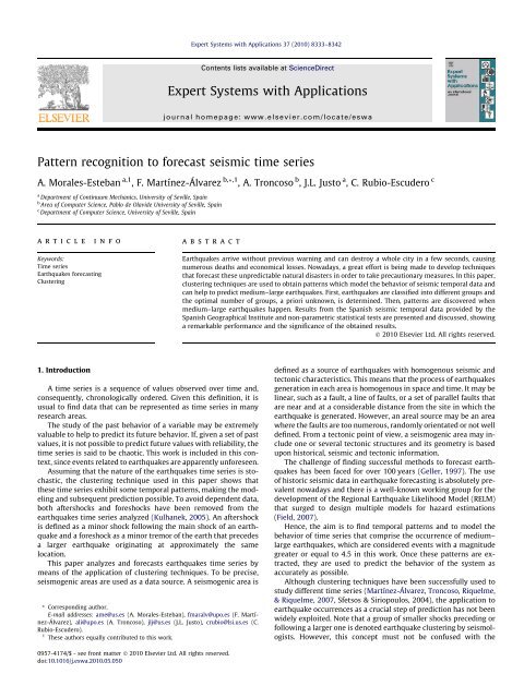
Expert Systems with Applications 37 (2010) 8333–8342Contents lists available at ScienceDirectExpert Systems with Applicationsjournal homepage: www.elsevier.com/locate/eswaPattern recognition to forecast seismic time seriesA. Morales-Esteban a,1 , F. Martínez-Álvarez b, * ,1 , A. Troncoso b , J.L. Justo a , C. Rubio-Escudero ca Department of Continuum Mechanics, University of Seville, Spainb Area of Computer Science, Pablo de Olavide University of Seville, Spainc Department of Computer Science, University of Seville, SpainarticleinfoabstractKeywords:Time seriesEarthquakes forecastingClusteringEarthquakes arrive without previous warning and can destroy a whole city in a few seconds, causingnumerous deaths and economical losses. Nowadays, a great effort is being made to develop techniquesthat forecast these unpredictable natural disasters in order to take precautionary measures. In this paper,clustering techniques are used to obtain patterns which model the behavior of seismic temporal data andcan help to predict medium–large earthquakes. First, earthquakes are classified into different groups andthe optimal number of groups, a priori unknown, is determined. Then, patterns are discovered whenmedium–large earthquakes happen. Results from the Spanish seismic temporal data provided by theSpanish Geographical Institute and non-parametric statistical tests are presented and discussed, showinga remarkable performance and the significance of the obtained results.Ó 2010 Elsevier Ltd. All rights reserved.1. IntroductionA time series is a sequence of values observed over time and,consequently, chronologically ordered. Given this definition, it isusual to find data that can be represented as time series in manyresearch areas.The study of the past behavior of a variable may be extremelyvaluable to help to predict its future behavior. If, given a set of pastvalues, it is not possible to predict future values with reliability, thetime series is said to be chaotic. This work is included in this context,since events related to earthquakes are apparently unforeseen.Assuming that the nature of the earthquakes time series is stochastic,the clustering technique used in this paper shows thatthese time series exhibit some temporal patterns, making the modelingand subsequent prediction possible. To avoid dependent data,both aftershocks and foreshocks have been removed from theearthquakes time series analyzed (Kulhanek, 2005). An aftershockis defined as a minor shock following the main shock of an earthquakeand a foreshock as a minor tremor of the earth that precedesa larger earthquake originating at approximately the samelocation.This paper analyzes and forecasts earthquakes time series bymeans of the application of clustering techniques. To be precise,seismogenic areas are used as a data source. A seismogenic area is* Corresponding author.E-mail addresses: ame@us.es (A. Morales-Esteban), fmaralv@upo.es (F. Martínez-Álvarez),ali@upo.es (A. Troncoso), jlj@us.es (J.L. Justo), crubio@lsi.us.es (C.Rubio-Escudero).1 These authors equally contributed to this work.defined as a source of earthquakes with homogenous seismic andtectonic characteristics. This means that the process of earthquakesgeneration in each area is homogenous in space and time. It may belinear, such as a fault, a line of faults, or a set of parallel faults thatare near and at a considerable distance from the site in which theearthquake is generated. However, an areal source may be an areawhere the faults are too numerous, randomly orientated or not welldefined. From a tectonic point of view, a seismogenic area may includeone or several tectonic structures and its geometry is basedupon historical, seismic and tectonic information.The challenge of finding successful methods to forecast earthquakeshas been faced for over 100 years (Geller, 1997). The useof historic seismic data in earthquake forecasting is absolutely prevalentnowadays and there is a well-known working group for thedevelopment of the Regional Earthquake Likelihood Model (RELM)that surged to design multiple models for hazard estimations(Field, 2007).Hence, the aim is to find temporal patterns and to model thebehavior of time series that comprise the occurrence of medium–large earthquakes, which are considered events with a magnitudegreater or equal to 4.5 in this work. Once these patterns are extracted,they are used to predict the behavior of the system asaccurately as possible.Although clustering techniques have been successfully used tostudy different time series (Martínez-Álvarez, Troncoso, Riquelme,& Riquelme, 2007, Sfetsos & Siriopoulos, 2004), the application toearthquake occurrences as a crucial step of prediction has not beenwidely exploited. Note that a group of smaller shocks preceding orfollowing a larger one is denoted earthquake clustering by seismologists.However, this concept must not be confused with the0957-4174/$ - see front matter Ó 2010 Elsevier Ltd. All rights reserved.doi:10.1016/j.eswa.2010.05.050

8334 A. Morales-Esteban et al. / Expert Systems with Applications 37 (2010) 8333–8342clustering techniques used in this paper, which are one of the maingoals of the Artificial Intelligence. In this sense, the novelty of thiswork lies on discovering clustering-based patterns and the use ofthem as seismological precursor in Spanish temporal data.Cluster analysis is the basis of many classification algorithmsthat provide models of systems (Xu & Wunsch, 2005). The mainaim of this analysis is to generate grouping of data from a largedataset with the intention of producing an accurate representationof the behavior of a system. Thus, these algorithms are focused onextracting useful information to find patterns in data.The rest of the work is divided as follows. Section 2 introducesthe methods used to predict the occurrence of earthquakes. TheSpanish seismic database is described in Section 3. The fundamentalsthat support the theory exposed in this work are presented inSection 4. Section 5 presents how the pattern recognition has beenperformed. Finally, the experimental results are shown in Section 6.2. Seismicity-based forecasting methodsMany authors have proposed different methods to predict theoccurrence of earthquakes. The work in Ward (2007) added fivedifferent models to the RELM. The first one, similar to the modelpresented in Kagan, Jackson, and Rong (2007), was based onsmoothed seismicity and predicted earthquakes with magnitudegreater or equal to 5.0. The second model is similar to the one proposedin Shen, Jackson, and Kagan (2007). The third is based onfault data analysis. The fourth model is a combination of the firstthree models and, finally, the last one is based on earthquake simulations(Ward, 2000).Kagan et al. (2007) have obtained forecasts of earthquakes withmagnitude greater or equal to 5.0 for five-years in Southern California.The forecasts were based on spatially smoothed historicalearthquake catalogue using the methodology described in Kaganand Jackson (1994).The authors in Helmstetter, Kagan, and Jackson (2007) havedeveloped a time-independent forecast for California by smoothedseismicity, similar to Kafka and Levin (2000), but including smallerevents and removing aftershocks. The working group on CaliforniaEarthquake Probability (Petersen, Cao, Campbell, & Frankel, 2007)has presented the Uniform California Earthquake Rupture Forecastversion 1 composed of four types of earthquake sources with distributedseismicity, similar to the National Seismic Hazard MapFrankel et al. (2002).Another forecast of five-years was provided by the AsperitybasedLikelihood Model (ALM), which assumes a Gutenberg–Richterdistribution of events (Wiemer & Schorlemmer, 2007) and considersthe size distribution of recent micro-earthquakes to be themost relevant information for predicting events of magnitudegreater or equal to 5.0.The Pattern Informatics model (Holliday et al., 2007) forecaststhe regions where earthquakes are most likely to occur in a nearfuture (5 to 10 years) by discovering zones with a high seismicactivity.Equally remarkable was the work in Shen et al. (2007), in whichthe authors developed a method based on geodetically observedstrain rate averaged over a time period, a decade concretely, forSouthern California.Bird and Liu (2007) proposed a two-step process for estimatinglong-term average seismicity of any region. The first step incorporatesall plate tectonic, geologic, geodetic and stress-direction datainto the model. The second one converts the deformation or momentrate into rate of earthquakes by applying the Seismic HazardInferred from Tectonics hypothesis, which states that the providedforecasts using the plate tectonic theory are more accurate thanthose based on past samples.Gerstenberguer, Jones, and Wiemer (2007) developed a methodto spatially map the probability of earthquake occurrences in 24 hbased on foreshock/aftershock statistics.The model in Rhoades (2007) performed forecasts for one yearbased on the notion that every earthquake is a precursor in accordancewith the scale. For this aim, the previous earthquakes ofminor magnitude were used to forecast those with major one.Finally, two forecasting methods were provided in Ebel, Chambers,Kafka, and Baglivo (2007). The first method was based on theassumption that the average of several statistical variables, such asspatial and temporal occurrences of earthquakes with magnitudegreater or equal to 4.0, during the forecasting period was the sameas the average of those variables over the past 70 years. The secondmethod used a hidden Markov model for making predictions forthe next day.The authors in Murru, Console, and Falcone (2009) presented ashort-term forecast model based on the propagation of aftershocksequences simulating the spreading of an epidemic.3. Description of the Spanish seismic dataThe database used for this study is the catalogue of SpanishGeographical Institute (SGI), which has calculated the locationand magnitude of Spanish earthquakes. The SGI has producedweekly and monthly catalogues for the area between 35N to 44Nand 10W to 5E.López and Muñoz (2003) reviewed how the magnitudes thatappear in the Spanish bulletins and catalogues were calculatedby the different authors that proposed them. The estimate of magnitudebased upon amplitude was obtained from Lg-wave registersor, generally, from the maximum train of the S-waves. The equationfor this estimate was corrected using a selection of earthquakes,whose magnitude had been measured by the UnitedStates Coast and Geodetic Survey (USCGS). Formerly, the difficultyin measuring the maximum amplitude for analog data, which producesunreliable magnitude estimates, encouraged some authorssuch as Tsumura (1967) to develop formulas based on the durationof their signals. Lee, Bennet, and Meagher (1972) defined a formulabased on trace duration between the arrival of the P-wave and theS-wave end. Owing to the development of these formulas, data recordedbefore 1962 were calculated using the earthquakes durationand after 1962, due to technological advances, usingamplitude and period of waves.Once aftershocks and foreshocks have been removed from thecatalogue, the first step is to determine the year of completenessof the catalogue for each area, defined as the year from which allthe earthquakes of magnitude equal or larger to M have been recorded.The year 1978 has been determined as the year of completenessfor Spanish seismic data in Justo Alpañés, Carrasco, andMartín Martín (1999).Magnitude estimates in the earthquake catalogue are nothomogeneous, because the calculation of the registers obtained before1962 was carried out using a different procedure. However,this does not have an effect on this study as only the registers from1978 onwards are used, because this is the completeness date ofthe seismic catalogue for magnitudes greater or equal to the cutoffmagnitude (Ranalli, 1969).The procedure used for the location of earthquakes is describedin Mezcua, Rueda, and García Blanco (2004). The location of theolder earthquake epicenters has been found graphically, usingisoseismic maps. The earthquake location has been found withthe application HYPO 71, based on the arrival time of the wavesto the stations and a model of the crust. Location errors have beenreduced from an average error of 25 km in 1964 to 3 km in 1996(see Giner, Molina, Jauregui, & Delgado, 2002).

8338 A. Morales-Esteban et al. / Expert Systems with Applications 37 (2010) 8333–8342Fig. 3. Seismogenic areas of Spain and Portugal.Mean silhouette values0.80.70.60.5Zone 26Zone 27Cluster1230.42 3 4 5 6 7 8 9 10Number of clustersFig. 4. Selection of the optimal number of clusters.0 0.2 0.4 0.6 0.8 1Silhouette Valuefive-earthquake groups that belong to the cluster 3, except for oneearthquake, occurred from the year 1993 to 1994, preceded by afive-earthquake group that belongs to the cluster 1. This onlyearthquake can be considered a separately case or an outlier forthis area.When the set of the preceding five-earthquakes was classifiedinto cluster 3, the mean magnitude of this set is low and the incrementof the b-value is positive according to the Table 2. When anearthquake of magnitude greater or equal to 4.5 occur, the groupof five-earthquakes including this large earthquake belongs tothe cluster 1. Therefore, it can be noted that the sequence of labelsthat characterize the earthquakes with magnitude greater or equalto 4.5 for this area is 3–1. The change of the membership from cluster3 to cluster 1 entails that the b-value decreases in a short time(from 1 to 2 months) nearby the occurrence of the shock (see Table2). Consequently, a decrease of the b-value is a precursor of earthquakesof magnitude greater or equal to 4.5 for the area ]26.Cluster123−0.2 0 0.2 0.4 0.6 0.8 1Silhouette ValueFig. 5. Silhouette index for three clusters in areas ]26 and ]27.

A. Morales-Esteban et al. / Expert Systems with Applications 37 (2010) 8333–8342 8339Table 2Centroids of the clusters.Area Cluster M Db Dt Membership (%)]26 ]1 3.56 0.047 0.16 34.38]2 3.39 0.013 0.83 9.38]3 3.28 +0.028 0.16 56.24]27 ]1 3.99 0.028 0.140 34.62]2 3.54 0.005 0.091 43.59]3 3.33 +0.035 0.519 21.79It can be observed that several five-earthquake groups withsmall magnitude are classified into the cluster 2, in which the b-valueis nearly constant and probably no important stress changesoccur.From Fig. 7, it can be stated that the seismogenic area ]27 followsa similar pattern to area ]26 until the year 2000. That is,the membership of five-earthquake groups to clusters changesfrom cluster 3 to 1 when a moderate–large earthquake occurs.Around the year 2000, a period of great tectonic activity take placewhere many earthquakes of magnitude greater or equal to 4.5 arerecorded. This period is characterized by short time intervals inwhich five–earthquake groups change their membership fromcluster 2 to 1, from cluster 1 to 2 and from cluster 1 to 1. However,all earthquakes of magnitude greater or equal to 4.5 (black circles)are classified into cluster 1 and most of them are preceded by five–earthquake groups that belong to the cluster 2 or 1 (sequences oflabels 2–1 and 1–1). It can be observed that most of precedingearthquakes classified into cluster 1 are, at the same time, precededby earthquakes that belong to the cluster 2. Let be 1–1 2the subset of earthquakes classified into the cluster 1 and precededby earthquakes belonging to the cluster 1 that are preceded byearthquakes classified into the cluster 2. Moreover, three earthquakeswith magnitude greater or equal to 4.5 classified into cluster1 also appeared in the last quarter of the year 2006. However,the preceding five-earthquake groups are not classified into thecluster 2 but into the cluster 3, in contrast to what it happens inthe 1–1 2 sequence. This sequence is denoted by 1–1 3 . Therefore,the sequences that characterize the earthquakes with magnitudegreater or equal to 4.5 for the area ]27 are 2–1, 1–1 2 and 1–1 3 .Thus, a decrease of the b-value is considered a precursor ofmoderate–large earthquakes for this area due to the change ofFig. 6. Clustering of earthquakes for the Alboran sea.Fig. 7. Clustering of earthquakes for the West Azores–Gibraltar fault.

8340 A. Morales-Esteban et al. / Expert Systems with Applications 37 (2010) 8333–8342membership of preceding earthquakes from cluster 3 to 1 in the sequence1–1 3 and from cluster 2 to 1 in the sequences 1–1 2 and 2–1(see Table 2).Moreover, it can be noticed that several earthquakes with smallmagnitude, occurring before the year 1995 with a longer period oftime among them, are classified into cluster 3 implying a large increaseof the b-value.In short, when a group of small earthquakes is classified into thecluster 3 or 2 and the b-value begins to decrease, the occurrence ofan earthquake with magnitude greater or equal to 4.5 in a near futureis forecasted and furthermore, this large earthquake will beclassified into the cluster 1.6.3. Quality of the resultsAll earthquakes with a magnitude greater or equal to 4.5 areclassified into cluster 1 and most of these earthquakes were precededby others belonging to cluster 3, cluster 2, sequence of clusters2–1 or sequence of clusters 3–1. Therefore, the sequences oflabels 3–1, 2–1, 1–1 2 and 1–1 3 are now going to be studied in orderto provide a measure of the quality of the obtained results in theprevious subsection.Table 3 provides the distribution of all earthquakes for differentclusters taking into consideration the cluster in which the precedingearthquakes are classified. The Hits columns identify thoseearthquakes that have magnitudes greater or equal to 4.5. It canstated that most of Hits are represented by sequences of labels3–1, 2–1 and 1–1 2 (13, 9 and 7, respectively).The last column makes reference to the existing ratio betweenthe number of earthquakes with magnitude greater or equal to4.5 classified into each sequence and the total occurrences of suchsequence. Note that the ratio corresponding to the sequences 3–1,2–1 and 1–1 2 are 0.65, 0.56 and 1, respectively. These values arethe highest ones among that of all sequences except for the sequence1–1 3 , which has a similar ratio to the ones in sequences3–1 and 2–1 (0.60 versus 0.65 and 0.56, respectively). Thus, the sequence1–1 3 is also considered to be representative, as it was statedin the previous section.True positives (TP) identify the occurrence of earthquakes withmagnitude greater or equal to 4.5 when any of the considered sequencesof labels are present. On the other hand, the false negatives(FN) represent the number of cases in which a medium–large earthquake also occurs but no proposed sequences of labelsare found. True negatives (TN) and false positives (FP) refer tothe situation in which no earthquakes occurred. However, the TNdenotes that no proposed sequences appear, while the FP makesreference to the apparition of any of the considered sequences.In addition, two well-known indices are provided, the sensitivityand the specificity. In this context, the sensitivity quantifies theTable 3Distribution of earthquakes into different sequences.Sequences Area #26 Area #27 RatioCases Hits Cases Hits1–1 1 7 1 3 3 0.401–1 2 1 0 6 7 11–1 3 4 0 1 3 0.601–2 1 0 14 0 01–3 16 0 2 0 02–1 2 0 14 9 0.562–2 2 0 16 2 0.112–3 5 0 4 1 0.113–1 17 9 3 4 0.653–2 6 0 4 0 03–3 35 0 10 0 0Total 96 10 77 29grade of reliability of the method when real events take placewhile the specificity measures the reliability of the method whensequences of labels are discarded. These indices are defined bythe following equations:Sensitivity ¼TPTP þ FN ;Specificity ¼TNFP þ TN :ð20Þð21ÞTable 4 measures the quality of the results obtained from the earthquakestemporal data distribution shown in Table 3. It can be observedthat the method obtains good levels of accuracy, sincesensitivities of 90.00% and 79.31% are reached for areas #26 and#27, respectively. Furthermore, the specificity reaches values greaterthan 80% and 90% for the areas #26 and #27, respectively. In short,not only medium–large earthquakes are detected with a good reliability,but also those cases in which earthquakes with a magnitudelesser than 4.5 appear are properly discarded. The obtained performanceis considered relevant for geophysical data analysts as theoccurrences of earthquakes present a high level of uncertainty.6.4. Statistical analysisThe well-known Wilcoxon rank-sum (WRS) test is applied in orderto show that the magnitude distributions of the earthquakesthat belong to the sequences 3–1, 2–1, 1–1 3 and 1–1 2 come fromthe same distribution with equal medians. The test has been appliedto all possible two–sequence combinations.The WRS is a standard non–parametric test for two independentsamples based on data ranking and it has been chosen because therequired conditions to apply parametric tests, such as normality ofdata, are not satisfied. A null hypothesis is an assumption about thepopulation to be tested. This hypothesis is accepted or rejected bythe test according to the p-value. When the p-value is lesser orgreater than a certain level of significance the hypothesis is rejectedor accepted, respectively. Therefore, the level of significanceis the probability of rejecting the null hypothesis being true. For instance,when the level of significance is 0.05, the probability ofmaking a mistake rejecting the null hypothesis is 5%.In this context, the samples are the maximum magnitudes ofthe groups of five-earthquakes classified into the cluster 1 for allsequences of clusters 3–1, 2–1, 1–1 3 and 1–1 2 versus the remainingsequences of two clusters. Therefore, the null hypothesis assumesthat these magnitudes are equally likely to occur. The level of significancehas been set to 0.05 as it is considered a typical level ofsignificance in most of statistical tests. The test has been appliedto the joining of all samples from both areas #26 and #27 sincethe number of the earthquakes classified into some of the sequences3–1, 2–1, 1–1 3 and 1–1 2 is not representatively enoughfor both areas separately. For instance, the sequence of labels 2–1 only appears twice in area #26 and the sequence 3–1 only appearsthree times in area #27.Table 5 shows the p-values obtained by the application of theWRS test to the samples for seismogenic areas #26 and #27, wherethe number in brackets represents the number of occurrences ofTable 4Results performance.Parameters Area #26 Area #27TP 9 23FN 1 6FP 15 5TN 71 47Sensitivity 90.00% 79.31%Specificity 82.56% 90.38%