Analytic design formulae for the design of reactive polymer blend ...

Journal of Membrane Science 360 (2010) 1–8Contents lists available at ScienceDirectJournal of Membrane Sciencejournal homepage: www.elsevier.com/locate/memsciAnalytic formulae for the design of reactive polymer blend barrier materialsS. Carranza, D.R. Paul, R.T. Bonnecaze ∗Department of Chemical Engineering, The University of Texas at Austin, 1 University Station CO400, Austin, TX 78712, United StatesarticleinfoabstractArticle history:Received 17 October 2009Received in revised form 13 April 2010Accepted 21 April 2010Available online 29 April 2010Keywords:Reactive membranesPackagingOxygen scavengingReactive particles that scavenge an undesirable permeate can be incorporated into thin plastic films tomake high performance composite barriers used as packaging materials. A multiscale model is presentedwith analytic solutions to the resulting equations to describe blends of non-spherical particles in thelimiting cases of fast and slow reaction rates. These analytic design formulae include predictions for thepermeate flux, time lag and kill time. In particular a quasi-steady permeate flux is quantified, which isobserved at early times when most reactive sites are still available. This flux can lead to significant leakageof the mobile species well before the time lag, and it is proposed as a critical figure of merit for the designof reactive barrier materials. The equation for the quasi-steady flux is valid for reactive particles of anyshape and requires only knowledge of average area to volume ratio for the particles within the blend inthe limit of fast reactions. The time lag is also shown to be valid for any polymer blends, irrespective ofparticle geometry, aspect ratio or reaction mechanism within the particle. The ranges of validity of thedesign formulae are found to be broad based on comparisons with numerical solutions of the model.© 2010 Elsevier B.V. All rights reserved.1. IntroductionPolymers are widely used as packaging materials that providechemically tunable barrier properties combined with goodmechanical properties and low cost. New polymer barrier materialsthat react or absorb undesirable permeates are being developed forproducts that are highly sensitive to oxygen or moisture, such asorganic light emitting diodes (OLEDs) for flexible displays [1–3]. Thecharacterization and validation of such reactive polymer materialsis challenging because they would provide barriers with lifetimeson the order of several years. In practice experiments for characterizationwould be done on much shorter time scales, and thusmodels are needed to extrapolate to long times to predict barrierperformance. The main purpose of this paper is to develop suchmodels for polymer blends.Oxygen scavenging polymers (OSPs), like polybutadiene, readilyoxidize [4–10]. However, scavenging polymers typically lackadequate structural properties so they are usually employed ascomposites with polymers such as poly(ethylene terephthalate)(PET) and polystyrene (PS). Polymer blends [11] and multilayercomposites [12–17] are two possible configurations of interest. Singlelayer reactive membranes have been modeled as homogeneoussystems [18–25], including the case of reactive particles uniformlydispersed in an inert media. A recent paper by Ferrari et al. [11] presenteda multiscale mathematical model describing the transport∗ Corresponding author. Tel.: +1 512 471 1497; fax: +1 512 471 7060.E-mail address: rtb@che.utexas.edu (R.T. Bonnecaze).of oxygen in a blend of spherical OSP particles within an inert polymermatrix. The system of non-linear partial differential equationswas solved numerically over a wide parameter space relevant topackaging applications.This paper significantly extends the methodology developedby Carranza et al. [26] for homogeneous reactive membranes toderive design formulae for polymer blends. It is also shown that thisanalytical approach can be easily adapted for blends to the practicallyimportant case of non-spherical particles. Furthermore, themethodology is demonstrated to accommodate variations in thekinetic model within the reactive particle, and in fact the functionalforms of the design equations obtained by asymptotic analysis areindependent of the details of the reactive term in the model equations.In particular the limits of fast and slow reactions within theparticles are considered here. The derivation of analytical designequations based on approximate solutions of the non-linear modeleliminates the need for lengthy simulations and provide clear relationshipsbetween critical design parameters and the physical andchemical properties of the polymer blend. In addition, extractionof parameters, such as diffusion and reaction coefficients, and sensitivityanalyses are made easier with analytical models.The results in this paper will be developed in the context of oxygenscavenging but in fact are generally applicable to any reactivepermeate and barrier system. Three regimes for the flux of oxygenwere observed in the numerical solutions of the multiscale model.At early times, an initial quasi-steady-state flux occurs. This leakageflux, though much smaller than that at true steady state when allthe scavengers have been consumed, is likely the most critical characteristicof such barrier materials. At intermediate times, the initial0376-7388/$ – see front matter © 2010 Elsevier B.V. All rights reserved.doi:10.1016/j.memsci.2010.04.029

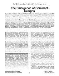
2 S. Carranza et al. / Journal of Membrane Science 360 (2010) 1–8Fig. 1. Schematic illustration of the polymer blend film and a particle in the limit of fast reaction.plateau gives way to a transient regime with increased oxygen flux,leading to the final regime, characterized by the time lag, when theflux approaches its steady-state value. Analytical estimates for theinitial flux plateau, for the intermediate transient flux, the time lagand kill time are presented along with their ranges of validity. Theextent and nature of the dependence of each regime on the particlegeometry and reactivity is discussed.2. Model descriptionConsider a membrane composed of reactive particles in an inertpolymer matrix, as illustrated schematically in Fig. 1. The matrix istypically an inert polymer with good mechanical properties, suchas poly(ethylene terephthalate) (PET) or polystyrene (PS), while theparticles are oxygen scavenging polymers (OSPs) such as polybutadiene(PB). As the matrix is inert, the reaction is confined to thescavenging particles. The particles and the matrix are assumed initiallydevoid of oxygen. A transport model at the particle-scale isfirst developed and then used to develop a multiscale transportmodel in a film of the blend.2.1. Particle modelThe reactive sites within each particle are immobilized and areconsumed as reaction progresses. Oxygen transport through theparticle obeys Fick’s law. Initially, the particles are devoid of oxygenand all reactive sites are available. The material balances, initial andboundary conditions for oxygen and the reactive materials withina spherical particle, for example, are given by∂C p∂t= D p ∂r 2 ∂r(r 2 ∂C p∂r)− k R nC p , (1)∂n∂t =−ˆk R nC p , (2)I.C. : C p (r, t = 0) = 0, n(r, t = 0) = n 0 ,B.C. : ∂C p∂r∣∣r=0= 0, C p (r = R, t) = C mH , (3)where C p is the oxygen concentration within the OSP particle, t istime, r is the radial position in spherical coordinates, D p is the oxygendiffusion coefficient within the particle, k R is the bulk reactionrate constant for reactive particle, n is the concentration of reactivesites, ˆ is the stoichiometric constant relating moles of oxygen tomoles of reactive sites, R is the radius of the OSP particle, C m is theconcentration of oxygen in the inert matrix, H = S m /S p is the partitioncoefficient relating the solubility of oxygen in the matrix S mto the solubility of oxygen oxidized OSP S p , and n 0 is initial concentrationof reactive sites. We will now consider the limiting cases ofvery fast reaction and very slow reaction.2.1.1. Reaction is much faster than diffusionDo [27] has shown that for cases where reaction is muchfaster than diffusion within the particle, i.e., the Thiele modulus˚p = (R 2 k R n 0 /D p ) 1/2 ≫ 1, the shrinking core model is valid. In theshrinking core model the reaction progresses as a moving front,consuming the immobilized sites behind the front, and leaving anunreacted shrinking core ahead of the front. The pseudo-steadystateconcentration at the particle’s moving front and the rate ofchange of the core radius are thus given by [11]:C p (a) = C mH(1 + k pa 2D p R( Ra − 1 ) ) −1, (4)(∂a=−ˆk p C m1 + k pa 2 ( R) ) −1∂t n 0 H D p R a − 1 , (5)where C m is the oxygen concentration in the inert matrix, k p is aneffective surface rate constant, a is the radius of the reactive coreand R is the radius of the OSP particle. The effective surface √ rateconstant in the moving front regime is given by k p = D p k R n 0 ,as shown √ in [26]. Sample calculations of the reactive length scaleL rxn = D p /k R n 0 = D p /k p , covering the range of values used innumerical calculations of Ferrari et al. [11], are shown in Table 1(note that in [11] the Damköhler number for the OSP particle isdefined by Da OSP = Rk P /D p = ˚p). These indicate the validity of theshrinking core model for much of the practical range of physicalparameters. However, as it will be discussed in the next sections,the specific form of Eq. (4) is only required for the derivation of theTable 1Sample calculations for OSP particles and blend for range of parameters used in [11].k p (cm/s) D p (cm 2 /s) R (m) L rxn (m) ˚p ˚bBase case 8 × 10 −5 2 × 10 −9 2.5 0.25 10 104Highest k p 1 × 10 −3 2 × 10 −9 2.5 0.02 125 367Low k p 1 × 10 −6 2 × 10 −9 2.5 20 0.1 12High D p 8 × 10 −5 2 × 10 −8 2.5 2.5 1 104Low D p 8 × 10 −5 2 × 10 −10 2.5 0.03 100 104High R 8 × 10 −5 2 × 10 −9 5.0 0.25 20 73Low R 8 × 10 −5 2 × 10√−9 0.5 0.25 2 231L rxn = D p/k p, ˚p = Rk P/D P, ˚b = 3k pL 2 /D mRH, where D m = 5.6 × 10 −9 cm 2 /s, H =1and L = 250 m for all cases above.

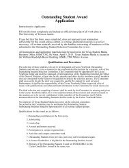
S. Carranza et al. / Journal of Membrane Science 360 (2010) 1–8 3Table 2Reactive sites material balance for various particle models. a .Shrinking core ˚p ≫ 1 Homogeneous ˚p ≪ 1Sphere = V 0/A 0k p, V 0/A 0 = R/3 = 1/k R n 0f (n/n 0) =∂n∂t , (11) ∂n(n/n 0 ) 2/3f (n/n 0) = n1+˚p((n/n 0 ) 1/3 −(n/n 0 ) 2/3 )n 0(n/n 0 ) 1/2f (n/n 0) = n1+˚p(n/n 0 ) 1/2 ln ((n/n 0 ) −1/2 )n 011+˚p(1−n/n 0 )√f (n/n 0) = nn 0R 2 k Rn 0/D p(n/n 0 ) 2/3, (6)1 + ˚p((n/n 0 ) 1/3 − (n/n 0 ) 2/3 )Cylinder = V 0/A 0k p, V 0/A 0 ∼ = R/2 = 1/kR n 0h 0 ≫ R f(n/n 0) =Disk = V 0/A 0k p, V 0/A 0 ∼ = h0/2 = 1/k R n 0h 0 ≪ R f(n/n 0) =√D p k Rn 0, ˚p = Rk p/D p =k p =aScavenger material balance is given by Eq. (12), ∂n =−ˆ C m∂t H f (n/n0).intermediate times regime, and variations of Eq. (4) can be easilyincluded in the model.Eq. (5) can be expressed in terms of the concentration of reactivesites n, which is proportional to the particle volume according to therelationship n/n 0 = V/V 0 = a 3 /R 3 , where n 0 is the initial concentrationof reactive sites, V 0 is the initial scavenger particle volumeand V is the volume of the unreacted core. Thus, the scavenger siteconcentration equation and initial condition are given by∂n=−ˆk pAC p=−ˆ 3k p C m∂t V 0 R HI.C. : n(t = 0) = n 0 , (7)where A = 4a 2 is the particle surface area at the moving front,V 0 = 4R 3 /3 is the initial volume of the particle and ˚p = Rk P /D Pis the Thiele modulus for the particle, expressed in terms of theeffective reactive rate constant k p . Equations similar to Eq. (6) canbe derived for shapes other than spheres and are listed in Table 2.2.1.2. Reaction is much slower than diffusionWhen reaction is much slower than diffusion, i.e., ˚p ≪ 1, thenthe concentration is uniform within the particle and the reactivesites are consumed uniformly over time [28]. Eqs. (1) and (2) andthe initial conditions reduce toC p = C mH , (8)∂n∂t =−ˆk C mR n, (9)HI.C. : n(t = 0) = n 0 . (10)2.2. Transport in the filmHere a model of the transport in the film of the blend is developedbased on the particle-scale reaction of oxygen with thescavengers. A schematic of the polymer blend of reactive particlesimbedded in an inert matrix is illustrated in Fig. 1. For packagingapplications the upstream side is exposed to an infinite source ofoxygen at partial pressure (p O2 ) 0at time t = 0. This source is typicallyair and the downstream side has vanishing oxygen partial pressure.The oxygen concentration at the gas/polymer interface is assumedto obey Henry’s law. The particles are assumed to be uniformly distributed,in large enough numbers and small enough compared tothe film thickness that average effective properties can be used. Theconcentration profile over the film takes into account the oxygenconsumption in each particle and the number density of particles inthe film. The non-linear transport equations in the reactive blend,along with initial and boundary conditions, are given by∂C m∂t= D m∂ 2 C m∂x 2+ ˆ=−ˆ C m∂t H f (n/n 0), (12)I.C. : C m (x, t = 0) = 0, n(x, t = 0) = n 0 , (13)B.C. : C m (0) ≡ C m (x = 0,t) = S m p O2 ,C m (L) ≡ C m (x = L, t) = 0. (14)where D m is the oxygen diffusion coefficient of the inert matrix and is the volume fraction of OSP in polymer blend. The characteristictime and the generic function of reactive sites concentrationf (n/n 0 ) depend on the reactive model chosen for the particle. Forspherical particles in the limit of ˚p ≫ 1, = R/3k p and f (n/n 0 ) =(n/n 0 ) 2/3 /(1 + ˚p((n/n 0 ) 1/3 − (n/n 0 ) 2/3 )), recovering Eq. (6).Inthelimit of ˚p ≪ 1, = 1/k R n 0 and f (n/n 0 ) = n/n 0 , recovering Eq.(9). Expressions for and f (n/n 0 ) for the two different models ofparticle-scale and particle shapes are given in Table 2. Note thatEq. (12) is the generic form of the material balance for reactivesites, which applies to both the homogeneous (slow reaction) andshrinking core (fast reaction) models of particles of any shape.The oxygen flux and the total amount of oxygen permeated arequantities of interest derived from the solution of Eqs. (11)–(14).The downstream flux J at time t is given by∣ J∣x=L =−D ∂Cm∂x ∣ , (15)x=Land the total oxygen permeated through the membrane Q t at timet is given by∫ tQ t = J| x=L dt. (16)0Numerical solutions of Eqs. (11)–(14) reveal three regimes ofinterest for the downstream flux (Fig. 2), as has been shown by Ferrariet al. [11]. The early time regime is characterized by a fast rise ofthe flux, followed by a flux plateau. This quasi-steady plateau eventuallygives way to a second regime of rising oxygen flux. The thirdregime occurs when all the reactive sites have been consumed, andthe flux reaches its final steady-state value. Note that the characteristictimes for each regime is independent of ˚p, as shown inFig. 2.The regimes observed in the transient downstream flux can bemapped to the concentration profiles, as illustrated in Fig. 3. Theearly time regime occurs before significant consumption of reactivesites. Most sites are still available, except for the region very closeto the upstream boundary. The uptake of oxygen in this regimecan be approximated by a simpler first-order reaction, as will bediscussed in the next section. For intermediate times, the concentrationprofiles can be divided into three zones. The first zone ispredominantly diffusive, characterized by a linear oxygen concentrationprofile, with all the reactive sites consumed. The secondzone shows a non-linear decay in the oxygen concentration due toreaction, coupled with a gradual change in reactive sites concentration.In the third zone, most reactive sites are still available, andthe oxygen concentration is vanishingly small, which is consistentwith the downstream boundary condition. A moving front developsduring this regime, leading to the analysis described in AppendixA to develop predictive equations for this regime. Note that thisis a front moving through the film and not to be confused withthe moving front within the reactive particle illustrated in Fig. 1.Finally, the third regime occurs when all the reactive sites havebeen consumed, and the concentration profile becomes linear overthe whole film. This regime is characterized by the time lag, whenthe flux approaches its steady-state value.The three regimes illustrated in Figs. 2 and 3 are observed forreactive transport in reactive polymer blends as well as homogeneousreactive membranes. The analytical solutions for these three

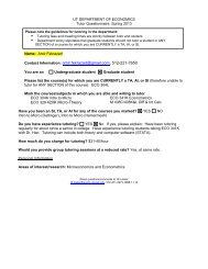
4 S. Carranza et al. / Journal of Membrane Science 360 (2010) 1–8Fig. 3. Concentration profiles for early, intermediate and long times.imated by the initial concentration of reactive sites n 0 . The oxygenflux in the plateau region of interest is also quasi-steady, and thus,the oxygen transport equation and boundary conditions becomeFig. 2. Comparison of numerical solution and analytical estimates for the threeregimes relevant to analysis of dimensionless downstream oxygen flux for = 0.0023, ˚b = 18 and (a) ˚p = 0.125, (b) ˚p = 1.25 and (c) ˚p = 12.5. Solutionsbased on shrinking core particle model (solid line = numerical solution, dashedline = prediction) and the bulk reaction particle model (dotted line = numerical solution,dash-dot = prediction) are compared. The initial flux plateau (horizontal dashedline) is the same for both models and matches closely the numerical solution. Insetshows the time lag as determined from the numerical solution, using the asymptoteas Q t→∞.regimes are derived for polymer blends in the next sections, followingthe framework described in Carranza et al. [26]. Table 3summarizes the approximate times for each time region in termsof the physical parameters of polymer blends for oxygen scavenging.Similar analysis could be extended to blends targeting otherspecies, e.g. water, by modifying the scavenging behavior accordingly.3. Analysis of early times to estimate initial leakage fluxplateauAt early times, most of the scavenger sites remain unreacted,except those very close to the upstream boundary, as illustrated inFig. 3. Therefore, the concentration of reactive sites n can be approx-d 2 C mdx 2− C m= 0, (17) HB.C. : C m (0) C m (x = 0,t) = S m p O2 ,C m (L) C m (x = L, t) = 0. (18)Table 3Analytical predictions of dimensionless flux for early, intermediate and long timesfor a reactive polymer blend.Time intervalEarly times aDimensional equationsJ| x=L = 2J SS˚b e −˚bt onset ≤ t ≤ t SFt onset = ((˚b − 1) H/2)√Intermediate times J| x=L = bJ SS (L/x F ) e −˚b (1−x F /L) , x F = 2 D m tt SF ≤ t ≤ t SF = H/2Long timesJ| x=L → J SS = C m(0)D m/Lt > √√= 0(1+3/)˚b = L 2 /D mH, ˚p = R 2 k R n 0/D p, = ˆC m(0)/n 0, 0 = L 2 /6D m. = 1/k R n 0 for ˚p ≪ 1, = V 0/A 0k p for ˚p ≫ 1.a J| x=L ∼ = 0 for t < tonset.

S. Carranza et al. / Journal of Membrane Science 360 (2010) 1–8 5Fig. 4. Parity chart for flux plateau comparing numerical solution and analytical predictionfor various ˚b and ˚p. The values in parenthesis give ˚b and ˚p, respectively,for each data point.This equation, along with the boundary conditions can be easilysolved to show thatC m =−C m (0) cosh(˛L)sinh(˛L) sinh(˛x) + C m(0) cosh(˛x), (19)√where ˛ = /H. Using Eq. (15) for the downstream flux withEq. (19) for oxygen concentration gives the following expressionfor the flux:∣∣J∣x=L = ˛LJ SS/sinh(˛L), or J∣x=L ∼2˛LJ SSe −˛L for ˛L ≫ 1, (20)where J SS is the steady-state oxygen flux Flux SS = J SS = C m (0)D m /L.Solovyov and Goldman [24] derived a similar equation for the fluxto describe a system with a large excess of reactive sites, as partof their modified moving front model. Here this model is used todescribe the flux in the early time regime.This equation can be expressed in terms of the √effective Thielemodulus for the film of the polymer blend ˚b = L 2 /D m H, i.e.,the ratio of the length scale of diffusion through the film and thelength scale of reaction within the particle so thatFlux plat = J| x=L = 2J SS˚b e −˚b , (21)which is valid for ˚b ≫ 1. This algebraic expression predicts theinitial flux plateau using physical properties that can be measuredexperimentally. Note that in the limit of ˚p ≪ 1, = 1/k R n 0 asshown in Table 2, thus making Eq. (21) independent of particleshape or surface area. In the limit of ˚p ≫ 1, = V 0 /A 0 k p in generalagain√regardless of particle shape as shown in Table 2, and thus˚b = A 0 k p L 2 /V 0 D m H. Therefore, the flux given by Eq. (21) isindependent of particle shape and depends only on the specific areaA 0 /V 0 in the limit of ˚p ≫ 1. In systems where particle shape cannotbe described by simple geometries, A 0 /V 0 can be determined byanalyzing images, e.g., by transmission electron microscopy, usingthe principles of stereology [29,30]. Eq. (21) is identical in functionalform in the limit of fast and slow reactions within the particles.Indeed the existence of the quasi-steady plateau flux is independentof the details of the reaction within the particle because atearly times all the scavenging sites are essentially accessible.The initial plateau estimate of Eq. (21) was compared to the valuesobtained by numerical solutions of the polymer blend modelequations and boundary conditions given by Eqs. (11)–(14) forboth fast and slow reactions. The prediction is in excellent agreementwith the numerical solutions for all the cases computed,as illustrated in Fig. 2 and the parity√plot of Fig. 4. The plateauflux decreases with increasing ˚b = L 2 /D m H, as illustratedin Fig. 5. The plateau flux is proportional to the steady-state fluxJ SS = C m (0)D m /L, and consequently to the upstream oxygen con-Fig. 5. Dimensionless downstream oxygen flux for = 0.0023 and various ˚b and˚p. The values in parenthesis give ˚b and ˚p, respectively, for each case. The plateauflux increases with decreasing ˚b, as predicted by Eq. (21). The initial plateau regionis bound by the plateau onset t onset and t SF, as predicted by Eqs. (22) and (23).,respectively.centration C m (0). Increasing D m increases J SS and decreases ˚b,leading to an increase in the initial flux plateau. Conversely, increasingL decreases J SS and increases ˚b, leading to a decrease in theinitial flux plateau. The increase in the flux due to increasing C m (0)or D m is expected, since the former causes more oxygen to be available,while the later enables fast transport of oxygen through thefilm, which leads to greater leakage through the film. Likewise, thedecrease due to higher L is also expected, since for thicker films, thediffusion time is longer, allowing the reaction to occur and, thus,reducing the amount of oxygen breakthrough at early times.The onset of the initial plateau t onset can be derived by recognizingthat the transient can be modeled as an unsteady first-orderreaction diffusion problem. This t onset is the time lag for an equivalentfirst-order reactive membrane, given by [26]:t onset = ˚b coth(˚b) − 1, or t onset ∼ = ˚b − 12/H2/H for ˚b ≫ 1. (22)Note that the second approximate expression for the onset timeretains the constant 1 in the numerator because it is found to be agood approximation for ˚b as low as 2 or 3.The initial plateau regime eventually transitions to a fast rise inthe downstream oxygen flux, in a transient regime described in thenext section. The transition between these two regimes occurs att SF , the time a steady front has been established. Following the stepsin [26], this time can be estimated by comparing the consumptionof reactive sites within the front volume with the influx of oxygeninto the front volume, and is given byt SF = H2 , (23)where = ˆC m (0)/ n 0 is the ratio between dissolved oxygenand reactive capacity. When the onset of the initial plateaut onset = t SF (˚b − 1) occurs before the steady front has been established,i.e., 0

6 S. Carranza et al. / Journal of Membrane Science 360 (2010) 1–8Table 4Values of b in Eq. (26) for flux estimate for blends of spherical particles with various˚p.˚p = (Rk P/D P) = (R 2 k Rn 0/D p) 1/2Homogeneous film 0.6530.1 0.5141 0.58110 1.54100 335tration equations are given by∂C m∂t= D m∂ 2 C m∂x 2− 3k pRC mH(n/n 0 ) 2/3, (24)1 + ˚p((n/n 0 ) 1/3 − (n/n 0 ) 2/3 )∂n∂t =−ˆ 3k p C m (n/n 0 ) 2/3. (25)R H 1 + ˚p((n/n 0 ) 1/3 − (n/n 0 ) 2/3 )Solutions in the frame of reference of the moving reaction zonewere developed, as shown in Appendix A, giving the algebraicexpression for the downstream flux:∣ J∣x=L = bJ L/x FSSe˚b (1−x F /L) , (26)where √ J SS = C m (0)D m /L is the steady-state oxygen flux andx F = 2 D m t is the position of the moving front. Values of bin Eq. (26), which are listed in Table 4 for spherical particles andvarious values of ˚p, are computed by numerical solutions of themoving front ODEs, as discussed in Appendix A. Note that thefunctional form of Eq. (26) is valid for a wide range of models, withspecific values of b computed for each different model. In the limitof ˚p ≪ 1 the transient result for the homogenous film is recoveredwhere b = 0.653 [26]. Fig. 2 compares the numerical solution to thepredicted values of the initial flux plateau [Eq. (21)] and the intermediatetransient flux [Eq. (26)] using the shrinking core particlemodel [Eqs. (24) and (25)] and the bulk reaction particle model[Eqs. (11) and (12) where = 1/k R n 0 and f (n/n 0 ) = n/n 0 ]. Thegraphs show the results for ˚p = 0.125, ˚p = 1.25 and ˚p = 12.5,where = 0.0023 and ˚b = 18 for all cases. Note that the resultsfor the shrinking core particle model and the bulk reaction particlemodel are nearly identical for ˚p = 0.125 and ˚p = 1.25, thereforeboth models can be used in this range of ˚p.As indicated in Table 3, the transient flux prediction of Eq. (26)is valid between the time a steady front has been established [t SFgiven by Eq. (23)] to the time before the front has reached the rightboundary, i.e., when most of the reactive sites have been consumed.Note that for larger ˚p (Fig. 2c) the flux increase from the initialplateau flux starts before t SF , resulting in a larger deviation fromthe predicted values.5. Figures of meritThe prediction of time lag for a reactive polymer blend wasderived in Ferrari et al. [11], following a method developed by Frisch[31], and adapted by Siegel and Cussler [18] to estimate the timelag for homogeneous reactive membranes. The expression derivedby Ferrari et al. is given by = 0 (1 + 3/), (27)where 0 = L 2 /6D m is the diffusion time lag of the inert matrix and = ˆC m (0)/n 0 is the ratio between dissolved oxygen and reactivecapacity. This algebraic equation for time lag was obtained assumingspherical particles, but is in fact generally valid irrespective ofthe shapes or sizes of the particles, and irrespective of the specificreaction mechanism within the particles. Note that the time lagbdepends only on the diffusion time scale through the inert matrix,and the ratio between dissolved oxygen and scavenging capacity ofthe blend.The cumulative oxygen permeate Q t is obtained by the integrationof the downstream flux, per Eq. (16), and can be estimatedanalytically by adding the contributions from the initial plateauregime, see Eq. (21), and the transient regime, see Eq. (26). Thus,the oxygen permeate can be estimated byQ t =∫ tSFt onset= 2J SSt SF ˚be˚b∫ tJ∣dt + x=Lt SF∣J∣x=L dt(1 + (1 − ˚b) + b (e√ t/tSF− e)) . (28)For times below t SF , the above equation reduces to the first integral,2J SS˚be −˚b (t + t SF (1 − ˚b)), which is the initial flux plateaumultiplied by t − t onset . The kill time t K , i.e., the time when theoxygen permeate reaches a predefined max Q max , proposed as atransient parameter in [22], can be found by solving Eq. (28) fortime, giving[t k = t SF ln 2 Qmax]e˚b 1 + (1 − ˚b)− + e . (29)2bJ SS t SF ˚b b6. Summary and conclusionsThe transport equations for a mobile permeate in a blend ofreactive particles in an inert matrix have been derived to describereactive particles of any shape in the limits of fast reaction andslow reaction. The framework developed to derive analytical designformulae for homogeneous reactive membranes [26] has beenextended to these reactive polymer blends, illustrating how theapproach can be adapted for models with very distinct reactiveterms. Equations for flux and characteristic times for the threeregimes identified in the numerical solutions have been derivedfor the polymer blend. It was found that the details of the reactionmechanism within the particles do not affect the functionalform of the analytic models and only affect the values of known oreasily determined constants in the predictive equations. The techniquepresented is broadly applicable and can be easily adapted toaccommodate other particle-scale reaction models.For the initial regime, when most reactive particles are still available,the initial plateau flux and plateau onset time t onset can bedetermined without knowledge of particle shapes, using insteadthe average area to volume ratio of the reactive particles A 0 /V 0 ,which can be determined by analyzing images using the principlesof stereology. Likewise, the characteristic time for the intermediateregime t SF , which marks the end of the initial flux plateau,requires only knowledge of A 0 /V 0 . One of the critical conclusionsof this paper is the generality of Eq. (21) for the prediction of thisflux. For many packaging applications, the initial plateau flux is theimportant design consideration because it characterizes the smallbut persistent leakage of oxygen through the barrier. Furthermore,the calculations for early times do not require the knowledge ofthe reaction details within the particle. The value of the downstreamflux for intermediate times can be predicted analyticallyif the particle shape is known. The third regime, when most particleshave been consumed, is characterized by the time lag andthe steady-state flux, which are completely independent of particleshape, area to volume ratios, or details of reaction within eachparticle.Traditionally, the time lag, which is independent of reaction rate,has been considered the figure of merit when designing reactivemembranes, as it marks the exhaustion of the reactive particles.However, this study suggests that the value of the initial fluxplateau, which accounts for both diffusion and reaction rates, along

S. Carranza et al. / Journal of Membrane Science 360 (2010) 1–8 7with its end time t SF are additional parameters to consider whendesigning packaging materials. For applications where it may bepreferable to design a barrier which will remain in the plateauregion throughout the life of the product, the end of the usefullife may be determined by the beginning of the transient regiont SF instead of time lag , and the value of the flux plateau can beused to determine the total permeate over the life of the product.AcknowledgmentThis work was supported in part by the National Science Foundationunder Grant Number DMR0423914.Appendix A.Following Carranza et al. [26], solutions in the frame of referenceof the moving reaction zone were developed, with solutions of theform:n(x, t)= (), (A.1)n 0C(x, t) = C m (0) =√Ht G(),(A.2)x − x F (t)√ , (A.3)D m H/where () represents the reactive site in the new frame of reference,G() is the self-similar oxygen √concentration field, H/ is thereactive time scale for the blend, D m H/ is the reactive lengthscale for the blend. The position of the moving front is given by√x F = 2 D m t, (A.4)where = ˆC m (0) / n 0 is the ratio between dissolved oxygen andreactive capacity. The leading order equations for the polymerblend becomed 2 Ĝ− Ĝf() = 0,d2 (A.5)d− Ĝf() = 0,d (A.6)B.C. : (∞) = 1, Ĝ(∞) = 0,dĜd ∣ =−1,−∞(A.7)where Ĝ = √ 2G.Provided that f () → 1as →∞, the asymptotic solutions ofthese equations as →∞are given byĜ = be − , = 1 − be − . (A.8)Thus, substituting Eq. (A.8) in Eq. (A.2) for concentration in themoving front regime and using Eq. (15) for flux gives Eq. (26), thealgebraic expression for the downstream flux. Note that Eq. (26)functional form is valid for any model with the asymptote f () → 1as →∞, regardless of the details of f (). If f () is known, thevalues of b may be computed by solving Eqs. (A.5) and (A.6) bythe shooting method using Eq. (A.8) as the initial conditions whilevarying b until the condition for matching the asymptotic solutionsof the diffusion zone and the moving reaction zone is satisfied, i.e.,Ĝ() =− as →−∞[26].Nomenclaturea radius of the reactive core, cmA area of scavenging core, cm 2A 0 area of scavenging particle, cm 2b constant for moving front flux prediction, dimensionlessC m O 2 concentration in the film, mol O2 /cm 3C m (0) oxygen concentration at the polymer blend filmupstream surface C m (0) = p O2 S m ,mol O2 /cm 3C p oxygen concentration in the OSP particle,mol O2 /cm 3 OSPD m oxygen diffusion coefficient of the inert matrix,cm 2 /sD p oxygen diffusion coefficient for the oxidized OSP,cm 2 /sf(n/n 0 ) reactive sites consumption function for a particleG variable for moving front analysis, dimensionlessĜ = √ 2GH partition coefficient, H = S m /S pJ oxygen flux, mol/cm 2 sk p reaction rate constant for reactive particle, cm/sk R bulk reaction rate constant for reactive particle,cm 3 OSP/mol RS sL thickness of the film, cmn concentration of reactive sites, mol RS /cm 3n 0 initial concentration of reactive sites, mol RS /cm 3p O2 oxygen partial pressure, MPaQ t oxygen permeate, mol/cm 2R radius of the OSP particle, cmS m solubility coefficient for oxygen in inert matrix,cm 3 (STP)/cm 3 MPaS p solubility coefficient for oxygen in the scavengingpolymer, cm 3 (STP)/cm 3 MPat time, st K kill time, st onset onset time for the initial flux plateau, st SF time when a steady moving front is established, sV volume of reactive core, cm 3V 0 volume of scavenging particle, cm 3x position along film thickness, cmx F moving front position, cmẋ F moving front speed, cm/s∼ denotes dimensionless variablesGreek lettersˇ OSP capacity, ˇ = n 0 /ˆ, mol O2 /cm 3 OSP time lag, s 0 diffusion time lag of inert polymer, 0 = L 2 /6D m ,s volume fraction of OSP in polymer blend˚b effective √ Thiele modulus for the blend,˚b = L 2 /D m H˚p Thiele√modulus for the OSP particle,˚p = R 2 k R n 0 /D p or ˚p = Rk p /D p reactive sites expressed in terms of moving frontcoordinate ratio between dissolved oxygen and reactive capacity, = ˆC m (0)/n 0ˆ stoichiometric coefficient, mol RS mol O2 time scale, = V 0 /A 0 k p or = 1/k R n 0 ,s moving front coordinate, dimensionless

8 S. Carranza et al. / Journal of Membrane Science 360 (2010) 1–8References[1] P.E. Burrows, et al., Gas permeation and lifetime tests on polymer-based barriercoatings, Proc. SPIE 4105 (2001) 75–83.[2] J. Lewis, Material challenge for flexible organic devices, Mater. Today 9 (2006)38–45.[3] M.C. Choi, Y. Kim, C.S. Ha, Polymers for flexible displays: from material selectionto device applications, Prog. Polym. Sci. 33 (2008) 581–630.[4] A.V. Tobolsky, D.J. Metz, R.B. Mesrobian, Low temperature autoxidation ofhydrocarbons: the phenomenon of maximum rates, J. Am. Chem. Soc. 72 (1950)1942–1952.[5] R.G. Bauman, S.H. Maron, Oxidation of polybutadiene. I. Rate of oxidation, J.Polym. Sci. 22 (1956) 1–12.[6] S.W. Beavan, D. Phillips, Mechanistic studies on the photo-oxidation of commercialpoly(butadiene), Eur. Polym. J. 10 (1974) 593–603.[7] J.F. Rabek, J. Lucki, B. Rånby, Comparative studies of reactions of commercialpolymers with molecular oxygen, singlet oxygen, atomic oxygen and ozone-I,Eur. Polym. J. 15 (1979) 1089–1100.[8] V.B. Ivanov, S.G. Burkova, Y.L. Morozov, V.Y. Shlyapintokh, Kinetics of thechain-propagation and chain-termination reactions in the oxidation of polybutadieneand copolymers of butadiene with styrene, Kinet. Katal. 20/5 (1979)1330–1333.[9] C. Adam, J. Lacoste, J. Lemaire, Photo-oxidation of elastomeric materials. Part 1-Photo-oxidation of polybutadienes, Polym. Degrad. Stabil. 24 (1989) 185–200.[10] M. Piton, A. Rivaton, Photooxidation of polybutadiene at long wavelengths( > 300 nm), Polym. Degrad. Stabil. 53 (1996) 343–359.[11] M.C. Ferrari, S. Carranza, R.T. Bonnecaze, K.K. Tung, B.D. Freeman, D.R. Paul,Modeling of oxygen scavenging for improved barrier behavior: blend films, J.Membr. Sci. 329 (2009) 183–192.[12] C.D. Mueller, S. Nazarenko, T. Ebeling, T.L. Schuman, A. Hiltner, E. Baer, Novelstructures by microlayer coextrusion—Talc-filled PP, PC/SAN, and HDPE/LLDPE,Polym. Eng. Sci. 37/2 (1997) 355–362.[13] E.E. Nuxoll, E.L. Cussler, Layered reactive barrier films, J. Membr. Sci. 252 (2005)29–36.[14] S.E. Solovyov, A.Y. Goldman, Optimized design of multilayer barrier films incorporatinga reactive layer. I. Methodology of ingress analysis, J. Appl. Polym. Sci.100 (2006) 1940–1951.[15] S.E. Solovyov, A.Y. Goldman, Optimized design of multilayer barrier films incorporatinga reactive layer. II. Solute dynamics in two-layer films, J. Appl. Polym.Sci. 100 (2006) 1952–1965.[16] S.E. Solovyov, A.Y. Goldman, Optimized design of multilayer barrier films incorporatinga reactive layer. III. Case analysis and generalized multilayer solutions,J. Appl. Polym. Sci. 100 (2006) 1966–1977.[17] S.E. Solovyov, A.Y. Goldman, Mass Transport Reactive Barriers in Packaging,DEStech Publications, Lancaster, PA, 2008.[18] R.A. Siegel, E.L. Cussler, Reactive barrier membranes: some theoretical observationsregarding the time lag and breakthrough curves, J. Membr. Sci. 229 (2004)33–41.[19] C. Yang, E.E. Nuxoll, E.L. Cussler, Reactive barrier films, AIChE J. 47/2 (2001)295–302.[20] C. Yang, E.L. Cussler, Oxygen barriers that use free radical chemistry, AIChE J.47/12 (2001) 2725–2732.[21] N.K. Lape, C. Yang, E.L. Cussler, Flake-filled reactive membranes, J. Membr. Sci.209 (2002) 271–282.[22] E.E. Nuxoll, E.L. Cussler, The third parameter in reactive barrier films, AIChE J.51/2 (2005) 456–463.[23] S.E. Solovyov, A.Y. Goldman, Theory of transient permeation through reactivebarrier films. I. Steady state theory for homogeneous passive and reactivemedia, Int. J. Polym. Mater. 54 (2005) 71–91.[24] S.E. Solovyov, A.Y. Goldman, Theory of transient permeation through reactivebarrier films. II. Two layer reactive-passive structures with dynamic interface,Int. J. Polym. Mater. 54 (2005) 93–115.[25] S.E. Solovyov, A.Y. Goldman, Theory of transient permeation through reactivebarrier films. III. Solute ingress dynamics and model lag times, Int. J. Polym.Mater. 54 (2005) 117–139.[26] S. Carranza, D.R. Paul, R.T. Bonnecaze, Design formulae for reactive barriermembranes, Chem. Eng. Sci. 65 (2010) 1151–1158.[27] D.D. Do, On the validity of the shrinking core model in noncatalytic gas solidreaction, Chem. Eng. Sci. 37/10 (1982) 1477–1481.[28] O. Levenspiel, Chemical Reaction Engineering, 3rd ed., John Wiley & Sons, NewYork, 1999.[29] G. Thomas, M.J. Goringe, Transmission Electron Microscopy of Materials, Wiley,New York, 1979.[30] J.C. Russ, R.T. Dehoff, Practical Stereology, 2nd ed., Kluwer Academic/PlenumPublishers, New York, 2000.[31] H.L. Frisch, The time lag in diffusion, J. Phys. Chem. 61 (1957) 93–95.