Dynamic price competition with capacity constraints and strategic ...

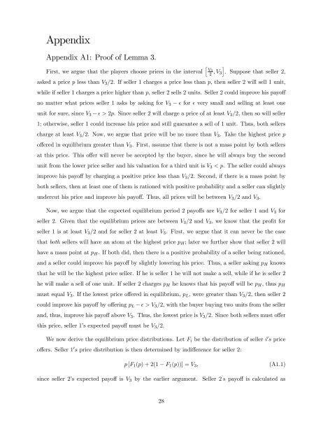
AppendixAppendix A1: Proof of Lemma 3.hFirst, we argue that the players choose prices in the interval V32,V 3i. Suppose that seller 2,asked a price p less than V 3 /2. Ifseller1 charges a price less than p, then seller 2 will sell 1 unit,while if seller 1 charges a price higher than p, seller2 sells 2 units. Seller 2 could improve his payoffno matter what prices seller 1 asks by asking for V 3 − ² for ² very small and selling at least oneunit for sure, since V 3 − ²>2p. Since seller 2 will charge a price of at least V 3 /2, thensowillseller1; otherwise, seller 1 could increase his price and still guarantee a sell of 1 unit. Thus, both sellerscharge at least V 3 /2. Now,wearguethatpricewillbenomorethanV 3 . Take the highest price poffered in equilibrium greater than V 3 . First, assume that there is not a mass point by both sellersat this price. This offer will never be accepted by the buyer, since he will always buy the secondunit from the lower price seller and his valuation for a third unit is V 3 V 3 /2, with the buyer buying two units from the sellerand, thus, improve his payoff above V 3 . Thus, the lowest price is V 3 /2. Since both sellers must offerthis price, seller 1’s expected payoff must be V 3 /2.We now derive the equilibrium price distributions. Let F i be the distribution of seller i 0 s priceoffers. Seller 1 0 s price distribution is then determined by indifference for seller 2:p [F 1 (p)+2(1− F 1 (p))] = V 3 ,since seller 2’s expected payoff is V 3 by the earlier argument.(A1.1)Seller 2 ’ spayoff is calculated as28