Dynamic price competition with capacity constraints and strategic ...
Dynamic price competition with capacity constraints and strategic ...
Dynamic price competition with capacity constraints and strategic ...

Create successful ePaper yourself
Turn your PDF publications into a flip-book with our unique Google optimized e-Paper software.
<strong>Dynamic</strong> <strong>price</strong> <strong>competition</strong> <strong>with</strong> <strong>capacity</strong> <strong>constraints</strong> <strong>and</strong><strong>strategic</strong> buyersGary Biglaiser 1University of North CarolinaNikolaos VettasAthens University of Economics <strong>and</strong> Business <strong>and</strong> CEPRJune 20, 20071 Biglaiser: Department of Economics, University of North Carolina, Chapel Hill, NC 27599-3305, USA;e-mail: gbiglais@email.unc.edu. Vettas: Department of Economics, Athens University of Economics <strong>and</strong>Business, 76 Patission Str., Athens 10434, Greece <strong>and</strong> CEPR, U.K.; e-mail: nvettas@aueb.gr. We are gratefulto the Editor <strong>and</strong> four anonymous referees of this Review <strong>and</strong> to Jim Anton, Luís Cabral, Jacques Crémer,Thomas Gehrig, Dan Kovenock, Jean-Jacques Laffont, Jean Tirole, Lucy White, Dennis Yao <strong>and</strong> seminarparticipants at various Universities <strong>and</strong> conferences for helpful comments <strong>and</strong> discussions. Parts of this workhave been completed while the first author was visiting the Portuguese Competition Authority - he gratefullyacknowledges the hospitality. Responsibility for all omissions <strong>and</strong> possible errors are, of course, only ours.
AbstractWe analyze a dynamic durable good oligopoly model where sellers are <strong>capacity</strong> constrained overthe length of the game. Buyers act <strong>strategic</strong>ally in the market, knowing that their purchases mayaffect future <strong>price</strong>s. The model is examined when there is one <strong>and</strong> multiple buyers. Sellers choosetheir capacities at the start of the game. We find that there are only mixed strategy equilibria.Buyers may split orders, preferring to buy a unit from both high <strong>and</strong> low <strong>price</strong> sellers to buying allunits from the low <strong>price</strong> seller. Sellers enjoy a rent above the amount needed to satisfy the marketdem<strong>and</strong> that the other seller cannot meet. Buyers would like to commit not to buy in the future orhire agents <strong>with</strong> instructions to always buy from the lowest <strong>price</strong>d seller. Further, sellers’ marketshares tend to be asymmetric <strong>with</strong> high probability, even though they are ex ante identical.JEL numbers: D4, L1Keywords: Strategic buyers, <strong>capacity</strong> <strong>constraints</strong>, bilateral oligopoly, dynamic <strong>competition</strong>.
1 IntroductionIn many durable goods markets, sellers who have market power <strong>and</strong> intertemporal <strong>capacity</strong> <strong>constraints</strong>face <strong>strategic</strong> buyers who make purchases over time. There may be a single buyer, as inthe case of a government that purchases military equipment or awards construction projects, suchas for bridges, roads, or airports, <strong>and</strong> chooses among the offers of a few large available suppliers.Or, there may be a small number of large buyers, such as in the case of airline companies thatorder aircraft or that of shipping companies that order cruise ships, where the supply could comeonly from a small number of large, specialized companies. 1 The <strong>capacity</strong> constraint may be dueto the production technology: a construction company undertaking to build a highway today maynot have enough engineers or machinery available to compete for an additional large project tomorrow,given that the projects take a long time to complete; a similar constraint is faced by anaircraft builder that accepts an order for a large number of aircraft. Or, the <strong>capacity</strong> constraintmaysimplycorrespondtotheflow of a resource that cannot exceed some level: thus, if a supplierreceives a large order today, he will be constrained on what he can offer in the future. This effectmay be indirect, if the resource is a necessary ingredient for a final product (as often in the caseof pharmaceuticals). More generally, cases like the ones mentioned above suggest a need to studydynamic oligopolistic <strong>price</strong> <strong>competition</strong> for durable goods under <strong>capacity</strong> <strong>constraints</strong>, when buyersare also <strong>strategic</strong>. Although this topic is both important <strong>and</strong> interesting, it has not been treatedyet in the literature.To obtain some first insights into the problem, consider the following simple setting. Take twosellers of some homogeneous product, say aircraft, to fix ideas. Each seller cannot supply morethan a given number of aircraft over two periods. Suppose that there is only one large buyer inthis market, this may be the Defense Department of some country, <strong>with</strong> a dem<strong>and</strong> that exceeds the<strong>capacity</strong> of each seller but not that of both sellers combined. Let the period one <strong>price</strong>s be lower1 Anton <strong>and</strong> Yao (1990) provide a critical survey of the empirical literature on <strong>competition</strong> in defenseprocurement - see also Burnett <strong>and</strong> Kovacic (1989) for an evaluation of relevant policies. In an empiricalstudy of the defense market, Greer <strong>and</strong> Liao (1986, p.1259) find that “the aerospace industry’s <strong>capacity</strong>utilization rate, which measures propensity to compete, has a significant impact on the variation of defensebusiness profitability <strong>and</strong> on the cost of acquiring major weapon systems under dual-source <strong>competition</strong>”.Ghemawat <strong>and</strong> McGahan (1998) show that order backlogs, that is, the inability of manufacturers to supplyproducts at the time the buyers want them, is important in the U.S. large turbine generator industry <strong>and</strong>affects firms’ <strong>strategic</strong> pricing decisions. Likewise, production may take significant time intervals in severalindustries: e.g., for large cruise ships, it can take three years to build a single ship <strong>and</strong> an additional two yearsor more to produce another one of the same type. Jofre-Bonet <strong>and</strong> Pesendorfer (2003) estimate a dynamicprocurement auction game for highway construction in California - they find that, due to contractors’ <strong>capacity</strong><strong>constraints</strong>, previously won uncompleted contracts reduce the probability of winning further contracts.1
for one seller than the other. Then, if the buyer’s purchases exhaust the <strong>capacity</strong> of the low <strong>price</strong>seller, only the other seller will remain active in the second period <strong>and</strong>, unconstrained from any<strong>competition</strong>, he will charge the monopoly <strong>price</strong>. A number of questions arise. Anticipating suchbehavior, how should the buyer behave? Should he split his orders in the first period, in order topreserve <strong>competition</strong> in the future, or should he get the best deal today? Given the buyer’s possibleincentives to split orders, how will the sellers behave in equilibrium? Should sellers <strong>price</strong> in a waythat would induce the buyer to split or not to split his purchases between the sellers? How dosellers’ equilibrium profits compare <strong>with</strong> the case of only a single pricing stage? Does the buyerhave an incentive to commit to not making purchases in the future? Are there incentives for thebuyer to vertically integrate <strong>with</strong> a seller? When there is more than one buyer, are the equilibriummarket shares of the (ex ante identical) sellers expected to be symmetric or asymmetric?We consider a set of simple dynamic models <strong>with</strong> the following key features. There are twoincumbent sellers who choose their capacities <strong>and</strong> a large number of potential sellers who can enter<strong>and</strong> choose their capacities after the incumbents. Capacity choices are, thus, endogenized <strong>and</strong>determine how much a firm can produce over the entire game. Next, sellers set first-period <strong>price</strong>s<strong>and</strong> then buyers decide how many units of the durable good they wish to purchase from each seller.The situation is repeated in the second period, given the remaining <strong>capacity</strong> of the firms; sellersset <strong>price</strong>s <strong>and</strong> buyers decide which firm to purchase from. We examine separately the cases of asingle buyer (monopsony) <strong>and</strong> that of two or more buyers (oligopsony).Our main results are as follows. First, entry is always blockaded - the <strong>capacity</strong> levels chosen bythe incumbent sellers are such that there is no profitable entry by other sellers. Given these <strong>capacity</strong>levels, a pure strategy subgame perfect equilibrium fails to exist. This is due to a combination oftwo phenomena. On the one h<strong>and</strong>, a buyer has an incentive to split his order in the first period ifthe <strong>price</strong>s are close, in order to keep strong <strong>competition</strong> in the second period. This in turn, givesthe sellers incentives to raise their <strong>price</strong>s. On the other h<strong>and</strong>, if <strong>price</strong>s get “high,” each seller has aunilateral incentive to lower his <strong>price</strong>, <strong>and</strong> sell all his <strong>capacity</strong>. We characterize the mixed strategyequilibrium <strong>and</strong> show that it has two important properties. Buyers have a strict incentive to splittheir orders <strong>with</strong> positive probability: for certain realizations of the equilibrium <strong>price</strong>s (that do notdiffer too much) a buyer chooses to buy in the first period from both a high <strong>price</strong> seller <strong>and</strong> a low<strong>price</strong> seller. Further, we also show that the sellers make a positive economic rent above the profitsof serving the buyer’s residual dem<strong>and</strong>, if the other seller sold all of his units. There are three mainimplications that follow from this result. First, buyers would like to commit to not make purchases2
in the second period, so as to induce strong <strong>price</strong> <strong>competition</strong> in the first period (that is, a buyeris hurt when <strong>competition</strong> takes place in two periods rather than in one). This is consistent <strong>with</strong>the practice in the airline industry, where airliners have options to buy airplanes in the future. Inparticular, the common practice of airline companies when they are purchasing aircraft is to ordera specific number (to be delivered over 2-4 years) <strong>and</strong> at the same time to agree on a significantnumber of “option aircraft”, <strong>with</strong> these options possible to be exercised over a specified time intervalof say 5-7 years. So, airline companies choose not to negotiate frequently <strong>with</strong> the sellers <strong>and</strong> placenew orders as their needs may increase over time, but instead they negotiate at one time in a waythat covers their possible needs over the foreseeable future. 2 Second, a buyer has the incentive toinstruct its purchasing agents to always buy from the lowest <strong>price</strong> firm. Thisisconsistent<strong>with</strong>many government procurement rules that do not allow discretion to its purchasing officers. In otherwords, in equilibrium, a buyer is hurt by his ability to behave <strong>strategic</strong>ally over the two periods <strong>and</strong>would like to commit to myopic behavior, if possible. Furthermore, buyers have a strict incentiveto vertically integrate <strong>with</strong> one of the suppliers. Finally, when there are multiple buyers, we findthat it is highly likely that sellers’ markets shares in both the first period <strong>and</strong> for the entire gamecan be quite asymmetric, even though sellers are ex ante identical.This paper studies <strong>competition</strong> <strong>with</strong> <strong>strategic</strong> buyers <strong>and</strong> sellers under dynamic (that is, intertemporal)<strong>capacity</strong> <strong>constraints</strong>. It is broadly related to two literatures. First, the literature on<strong>capacity</strong>-constrained <strong>competition</strong> starts <strong>with</strong> the classic work of Edgeworth (1897) who shows that<strong>competition</strong> may lead to the “nonexistence” of a <strong>price</strong> equilibrium or, as is sometimes described,<strong>price</strong> “cycles”. Subsequent work that has studied pricing under <strong>capacity</strong> <strong>constraints</strong> includes Beckman(1965), Levitan <strong>and</strong> Shubik (1972), Osborne <strong>and</strong> Pitchik (1986) <strong>and</strong> Dasgupta <strong>and</strong> Maskin(1986b). 3 Other papers have studied the choice of capacities in anticipation of oligopoly competi-2 This is common practice in the industry. For example, in 2002 EasyJet signed a contract <strong>with</strong> Airbus for120 new A319 aircraft <strong>and</strong> also for the option to buy, in addition, up to an equal number of such aircraft for(about) the same <strong>price</strong>. While the agreed aircraft were being gradually delivered, in 2006 EasyJet exercisedthe option <strong>and</strong> placed an order for an additional 20 units to account for projected growth, <strong>with</strong> delivery setbetween then <strong>and</strong> 2008. Similarly, an order was placed in 2006 by GE Commercial Aviation to buy 30 Nextgeneration 737s from Boeing <strong>and</strong> also to agree for an option for an additional 30 such aircraft.3 Kirman <strong>and</strong> Sobel (1974) prove equilibrium existence in a dynamic oligopoly model <strong>with</strong> inventories.Gehrig (1990, ch.2) studies non-linear pricing <strong>with</strong> <strong>capacity</strong> constrained sellers. Lang <strong>and</strong> Rosenthal (1991)characterize mixed strategy <strong>price</strong> equilibria in a game where contractors face increasing cost for each additionalunit they supply.3
tion 4 <strong>and</strong> the effect of <strong>capacity</strong> <strong>constraints</strong> on collusion. 5 All this work refers to <strong>capacity</strong> <strong>constraints</strong>that operate period-by-period, that is, there is a limit on how much can be produced or sold in eachperiod that does not depend on past decisions. <strong>Dynamic</strong> <strong>capacity</strong> <strong>constraints</strong>, the focus of our paper,have received much less attention in the literature. Griesmer <strong>and</strong> Shubik (1963), <strong>with</strong> <strong>price</strong>s ina discrete set <strong>and</strong> Dudey (1992), allowing <strong>price</strong>s to vary continuously, study games where <strong>capacity</strong>constrainedduopolists face a finite sequence of identical buyers <strong>with</strong> unit dem<strong>and</strong>s. Under certainconditions, the equilibrium has sellers maximizing their joint profits. Ghemawat (1997, ch.2) <strong>and</strong>Ghemawat <strong>and</strong> McGaham (1998) characterize mixed strategy equilibria in a two-period duopoly(<strong>with</strong> one seller having initially half of the <strong>capacity</strong> of the other). Garcia, Reitzes, <strong>and</strong> Stacchetti(2001) examine hydro-electric plants that can use their <strong>capacity</strong> (water reservoir) or save it for usein a later period. Dudey (2006) presents conditions so that a Bertr<strong>and</strong> outcome is consistent <strong>with</strong>capacities chosen by the sellers before the buyers arrive. In the above mentioned papers, dem<strong>and</strong>is modeled as static <strong>and</strong> independent across periods. The key distinguishing feature of our work isthat the buyers (<strong>and</strong> not just the sellers) are <strong>strategic</strong> <strong>and</strong> the evolution of capacities across periodsdepends on the actions of both sides of the market. 6Second, the present paper is related to the body of research where both buyers <strong>and</strong> sellers arelarge <strong>and</strong> <strong>strategic</strong>. 7 In particular, it is related to other work that examines when a buyer influencesthe degree of <strong>competition</strong> among (potential) suppliers, as in the context of “split awards” <strong>and</strong> “dualsourcing”.Rob (1986) studies procurement contracts that allow selection of an efficient supplier,while providing incentives for product development. Anton <strong>and</strong> Yao (1987, 1989, <strong>and</strong> 1992) considermodels where a buyer can buy either from one seller or split his order <strong>and</strong> buy from two sellers, whohave strictly convex cost functions. They find conditions under which a buyer will split his order4 See e.g. Dixit (1980), Spulber (1981), Kreps <strong>and</strong> Scheinkman (1984), Davidson <strong>and</strong> Deneckere (1986),<strong>and</strong> Allen, Deneckere, Faith, <strong>and</strong> Kovenock (2000) to mention a few.5 See e.g. Brock <strong>and</strong> Scheinkman (1985), Lambson (1987), <strong>and</strong> Compte, Jenny <strong>and</strong> Rey (2002).6 In recent work, Bhaskar (2001) shows that, by acting <strong>strategic</strong>ally, a buyer can increase his net surpluswhen sellers are <strong>capacity</strong> constrained. In his model, however, there is a single buyer who has unit dem<strong>and</strong>in each period for a perishable good, <strong>and</strong> so “order splitting” cannot be studied: the buyer can chose not tobuy in a given period, thus receiving zero value in that period, but gets future units at lower <strong>price</strong>s. Ourmodel allows both for a single <strong>and</strong> for multiple buyers. Buyers view the good as durable (receive value overboth periods) <strong>and</strong> may wish to split their orders, possibly buying from the more expensive supplier in thefirst period. Our focus <strong>and</strong> set of results are, thus, quite different. Equilibrium behavior is such that thebuyers get hurt as a result of their <strong>strategic</strong> behavior because it alters the pricing incentives for the sellers.In our model, in equilibrium a buyer never chooses not to buy any units in the first period.7 Aspects of bilateral oligopoly have been studied, among other papers, in Horn <strong>and</strong> Wolinsky (1988),Dobson <strong>and</strong> Waterson (1997), Hendricks <strong>and</strong> McAfee (2000) <strong>and</strong> Inderst <strong>and</strong> Wey (2003).4
consumption value V in each period. We assume that V ≥ V 3 > 0. 9At the start of the game the incumbent sellers simultaneously choose their capacities. Thepotential entrants observe the incumbents’ <strong>capacity</strong> choices <strong>and</strong> then simultaneously choose whetherto enter <strong>and</strong> their <strong>capacity</strong> choice if they enter. We assume that the cost of <strong>capacity</strong> for any seller issmall, ε, but positive. The marginal cost of production is 0 if total sales across both selling periodsone <strong>and</strong> two do not exceed <strong>capacity</strong> <strong>and</strong> infinite otherwise. 10 The <strong>capacity</strong> choice is the maximumthat the seller can produce over the two periods. Thus, each seller has <strong>capacity</strong> at the beginningof the second period equal to his initial <strong>capacity</strong> less the units he sold in the first period.Throughout the analysis, we will examine subgames where the <strong>capacity</strong> choice at the start ofthe game for each incumbent seller is equal to 3N − 1, whereN is the number of buyers (e.g.in monopsony each seller has 2 units <strong>and</strong> in duopsony each seller has 5 units) <strong>and</strong> that entry isalways blockaded. We demonstrate that these are the equilibrium <strong>capacity</strong> choices when we workvia backward induction in the analysis.In each period, each of the sellers sets a per unit <strong>price</strong> for his available units of <strong>capacity</strong>. 11 Eachbuyer chooses how many units he wants to purchase from each seller at the <strong>price</strong> specified, as longas the seller has enough <strong>capacity</strong>. If the dem<strong>and</strong> by buyers is greater than a seller’s <strong>capacity</strong>, thenthey are rationed. The rationing rule that we use is that each buyer is equally likely to get hisorder filled. The rationed buyers can buy from the other seller as many units as they want. 12 Weassume that sellers commit to their <strong>price</strong>s one period at a time <strong>and</strong> that all information is commonknowledge <strong>and</strong> symmetric. We are looking for symmetric subgame perfect equilibria of the game.Let us now discuss why we have adopted this modelling strategy. We analyze a dynamic bilateral9 To clarify, the maximum gross value that a buyer could obtain over both periods <strong>and</strong> evaluated at thebeginning of the first period is equal to 2V (1+δ)+δV 3 . Our specification is consistent <strong>with</strong> growing dem<strong>and</strong>.Note that, in general, the first <strong>and</strong> second units could have different values (say V 1 ≥ V 2 ). Also, we couldallow the dem<strong>and</strong> of the third unit to be r<strong>and</strong>om. It is straightforward to introduce either of these cases inthe model, <strong>with</strong> no qualitatitive change in the results, only at the cost of some additional notation.10 It will be clear that if the marginal cost of producing an additional unit above the intial <strong>capacity</strong> level,2formonoposony,issufficiently high, then the results still hold. Also, fixed costs would not change theresults as long as fixed costs are below a seller’s equilibrium profit. If the fixed costs were above a seller’sequilibrium profit, then the firm would not enter.11 We focus on the core case where each seller sets a simple unit <strong>price</strong>, that is <strong>competition</strong> when thereis no <strong>price</strong> discrimination among buyers or among units. The flavor of our results would be the same ifdiscriminatory pricing was allowed <strong>with</strong> multiple buyers.12 Our results would not change qualitatively if the sellers could choose which buyer to ration, as long aseach buyer has a positive probability of being rationed.6
oligopoly game, where all players are “large” <strong>and</strong> are therefore expected to have market power. Insuch cases, one wants the model to reflect the possibility that each player can exercise some marketpower. By allowing the sellers to make <strong>price</strong> offers <strong>and</strong> the buyers to choose how many units toaccept from each seller, all players have market power in our model. It follows that quantities <strong>and</strong><strong>price</strong>s evolve from the first period to the second jointly determined by the strategies adopted by thebuyers <strong>and</strong> the sellers. If, instead, we allowed the buyers to make <strong>price</strong> offers, then the buyers wouldhave all the market power <strong>and</strong> the <strong>price</strong> would be zero. This would not be realistic, particularly inthe case when there are at least as many buyers as sellers. 13 In fact, anticipating such a scenario,sellers would not be willing to pay even an infinitesimal entry cost <strong>and</strong>, thus, such a market wouldnever open. 14 There are further advantages of this modeling strategy. First, it makes the resultseasy to compare between the monopsony <strong>and</strong> the oligopsony cases. Second, it makes our resultsmore easily comparable <strong>with</strong> other papers in the literature, in particular the ones mentioned in theIntroduction <strong>with</strong> intertemporal <strong>capacity</strong> <strong>constraints</strong>, where the <strong>price</strong>s are indeed set by the sellers.Third, there may be agency (moral hazard) considerations that contribute to why in practice wetypically see the sellers making offers. 15 We note, that in any games <strong>with</strong> multiple players on bothsides of the market there are many possible game forms. We have chosen a natural one as a startingpoint to examine the issues that we are investigating.The interpretation of the timing of the game is immediate in case the sellers’ supply comes froman existing stock (either units that have been produced at an earlier time, or some natural resourcethat the firm controls). One simple way to underst<strong>and</strong> the timing in the case where production13 Inderst (2006) demonstrates that giving multiple buyers the right to make offers generates interestingresults due to the convexity of the sellers’ cost functions for all units. In our model of constant marginalcosts for all units where a seller has <strong>capacity</strong> in place, the buyer will always buy a unit at a <strong>price</strong> of 0 if thebuyers can make offers.14 Of course, there are other structures that would allow buyers <strong>and</strong> sellers to each keep part of themarket surplus, involving some form of multilateral bargaining. However these appear less robust <strong>and</strong> morecomplicated (<strong>and</strong> in particular, dependent on the exact modeling details) than the structure we have adoptedhere. In any game where the sellers would have some control over setting <strong>price</strong>s <strong>and</strong> the buyers over choosingwhere to buy from, it is expected that equilibrium behavior would reflect the same qualitative features weemphasize here.15 In general we see the sellers making offers, even <strong>with</strong> a single buyer, like when the Department of Defense(DOD) is purchasing weapon systems. The DOD may do this to solve possible agency problems betweenthe agent running the procurement auction <strong>and</strong> the DOD. If an agent can propose offers, it is much easierfor sellers to bribe the agent to make high offers than if sellers make offers, which can be observed by theregulator. This is because the sellers can bribe the agent to make high offers to each of them, but <strong>competition</strong>between the sellers would give each seller an incentive to submit a bid to make all the sells <strong>and</strong> it would bequite difficult for the agent to accept one offer that was much higher than another.7
t = 0 t = 1 t = 2Production of units ordered at t = 1Production of units ordered at t = 2Sellersset<strong>price</strong>sBuyers placetheir orders.Production ofunits ordered inperiod 1 starts.Sellersset<strong>price</strong>sBuyers place theirorders.Production ofunits ordered inperiod 2 starts.Figure 1: Timingtakes place in every period is illustrated in Figure 1. The idea here is that actual production takestime. Thus, orders placed in period 1 are not completed before period two orders arrive. Sinceeach seller has the <strong>capacity</strong> to work only on a limited number of units at a time, units orderedin period one restrict how many units could be ordered in period two. In such a case, since ourinterpretation involves delivery after the current period, the buyers’ values specified in the gameshould be understood as the present values for these future deliveries (<strong>and</strong> the interpretation ofdiscounting should also be accordingly adjusted).3 MonopsonyWe first examine the single buyer case (N =1), that is, monopsony. We are constructing a subgameperfect equilibrium, <strong>and</strong> thus we work backwards by starting from period 2.3.1 Second periodThere are several cases to consider, depending on how many units the buyer has bought from eachseller in period one. We will use, throughout the paper, the convention of calling a seller <strong>with</strong> iunits of remaining <strong>capacity</strong> seller i.Buyer bought two units in period 1. If the buyer bought a unit from each of the sellers in period1, then the <strong>price</strong> in period 2 is 0 due to Bertr<strong>and</strong> <strong>competition</strong>. If the buyer bought both units fromthe same firm, then the other firm would be a monopolist in period 2 <strong>and</strong> charge V 3 .Thus,period2 equilibrium profit of a seller that has one remaining unit of <strong>capacity</strong> is 0 <strong>and</strong> that of a seller <strong>with</strong>two remaining units of <strong>capacity</strong> is V 3 .Buyer bought one unit in period 1. In this case, the buyer has dem<strong>and</strong> for two units, one of8
the sellers has a <strong>capacity</strong> of 1 unit, seller 1, while the other has a <strong>capacity</strong> of 2 units, seller 2. Wedemonstrate that there is no pure strategy equilibrium in period 2 by the following Lemma.Lemma 1 If the buyer bought one unit in period 1 in the monopsony model, then there is no purestrategy equilibrium in period 2.Proof. First, notice that the equilibrium cannot involve seller 2 charging a zero <strong>price</strong>: thatseller could increase his profit by raising his <strong>price</strong> (as seller 1 does not have enough <strong>capacity</strong> tocover the buyer’s entire dem<strong>and</strong>). Thus, seller 1 would also never charge a <strong>price</strong> of zero. Supposenow that both sellers charged the same positive <strong>price</strong>. One, if not both, sellers have a positiveprobability of being rationed. A rationed seller could defect <strong>with</strong> a slightly lower <strong>price</strong> <strong>and</strong> raisehis payoff. Suppose that the <strong>price</strong>s are not equal: p i
We obtain two key insights from Lemma 2 that run throughout the paper. The first concerns thecalculation of the equilibrium sellers’ profits <strong>and</strong> the second regards the ranking of the sellers’ <strong>price</strong>distributions. The high <strong>capacity</strong> seller can always guarantee himself a payoff of at least V 3 (B − C),since he knows that, no matter what the other seller does, he can always charge V 3 <strong>and</strong> sell at leastB − C units. This is the high-<strong>capacity</strong> seller’s security profit level. This is because the low-<strong>capacity</strong>seller can supply only up to C of the B units that the buyer dem<strong>and</strong>s <strong>and</strong> the buyer is willing topay up to V 3 . This high-<strong>capacity</strong> seller’s security profit puts a lower bound on the <strong>price</strong> offered inperiod 2. Given the high-<strong>capacity</strong> seller can sell at most B units (that is, the total dem<strong>and</strong>), hewill never charge a <strong>price</strong> below V 3 (B − C)/B, since a lower <strong>price</strong> would lead to profit lessthanhissecurity profit. Since the high-<strong>capacity</strong> seller would never change a <strong>price</strong> below V 3 (B − C)/B, thislevel also puts a lower bound on the <strong>price</strong> the low-<strong>capacity</strong> seller would charge <strong>and</strong>, as that sellerhas C units he could possibly sell, his profit isatleastC V 3(B−C)Bhis security profit. 17 Competitionbetween the two sellers fixes their profits at their respective security levels. 18The second insight deals <strong>with</strong> the incentives for aggressive pricing. We find that the seller <strong>with</strong>larger <strong>capacity</strong> will <strong>price</strong> less aggressively than the seller <strong>with</strong> smaller <strong>capacity</strong> in period 2. Thelarger <strong>capacity</strong> seller knows that he will make sales even if he is the highest <strong>price</strong> seller, whilethe smaller <strong>capacity</strong> seller makes no sales if he is the highest <strong>price</strong> seller. So, the low <strong>capacity</strong>seller always has incentives to <strong>price</strong> more aggressively. More precisely, the high-<strong>capacity</strong> seller <strong>price</strong>distribution first-order stochastically dominates the <strong>price</strong> distribution of the low <strong>capacity</strong> seller.This general property has important implications for the quantities sold <strong>and</strong> the market sharesover the entire game.For the special case of interest here, <strong>with</strong> a single buyer, we have: 19Lemma 3 If the buyer bought one unit in period 1 in the monopsony model, then there is a uniquemixed strategy equilibrium. Both sellers mix on the interval [V 3 /2,V 3 ] . Seller 1 0 s <strong>price</strong> distributionis F 1 (p) =2− V 3p, <strong>with</strong> an expected profit ofV 3 /2. Seller 2 0 s <strong>price</strong> distribution is F 2 (p) =1− V 32p forp
1F 11 2F 2V32V3pFigure 2: Mixed strategy equilibrium <strong>with</strong> asymmetric capacitiesfirst order stochastically dominates seller 1’s distribution.Figure 2 illustrates the <strong>price</strong> distributions in this case.We now examine the remaining period-two case (subgame).Buyer bought no units in period 1. Each seller enters period 2 <strong>with</strong> 2 units of <strong>capacity</strong>, whilethe buyer dem<strong>and</strong>s 3 units. Using argument along the lines used for Lemma 2, each player’sexpected second-period equilibrium profit willbeequaltoV 3 , the security profit ofeachseller. Theequilibrium behavior in the second period is now summarized:Lemma 4 Second period <strong>competition</strong> for a monopsonist falls into one of three categories. (i) Ifonly one seller is active (the rival has zero remaining <strong>capacity</strong>), that seller sets the monopoly <strong>price</strong>,V 3 , <strong>and</strong> extracts the buyer’s entire surplus. (ii) If each seller has enough <strong>capacity</strong> to cover by himselfthe buyer’s dem<strong>and</strong> then the <strong>price</strong> is zero. (iii) If the buyer’s dem<strong>and</strong> exceeds the <strong>capacity</strong> of oneseller but not the aggregate sellers’ <strong>capacity</strong>, then there is no pure strategy equilibrium. In the mixedstrategy equilibrium, a seller <strong>with</strong> two units of <strong>capacity</strong> has expected profit equaltoV 3 <strong>and</strong> a seller<strong>with</strong> one unit of <strong>capacity</strong> has expected profit equaltoV 3 /2.3.2 First periodNow, we go back to period 1. First, we demonstrate that the buyer will always buy two unitsin equilibrium <strong>and</strong> that there is no pure strategy equilibrium. We then characterize equilibriumpayoffs <strong>and</strong> discuss the properties of equilibria.Proposition 1 The buyer buys two units in period 1.11
We sketch the proof here; the formal proof is in Appendix A2. First, <strong>price</strong>s must be positive,sincethesellerknowsthatevenifhedoesnotsellaunitinperiod1,hewillmakepositiveprofitsin period 2. We then show that a buyer will never buy three units in period 1. For the buyer tobuy three units, he must buy two units from the low <strong>price</strong> seller at a positive <strong>price</strong> <strong>and</strong> one fromthe other seller. If he only buys one unit from each seller in period 1, the <strong>price</strong> for the third unitbought in period 2 is zero due to Bertr<strong>and</strong> <strong>competition</strong>; thus, the buyer will never buy three units.We next argue that the <strong>price</strong> never exceeds a bound such that the buyer prefers buying one unitfrom each seller as opposed to only one unit from the low <strong>price</strong> seller. This is because this <strong>price</strong> isgreater than δV 3 , which by Lemma 4 is greater than a seller’s expected profit inperiod2 if he makesno sales in period 1. Thus, two units will always be purchased in any equilibrium. An importantimplication for this result is that production is always efficient: the buyer always gets units whenhe needs them.A feature of the equilibrium is the incentive of the buyer to split his order. This is captured bythe following result.Lemma 5 The buyer prefers to buy one unit from each seller as opposed to buying two units fromthe lowest <strong>price</strong> seller if the difference in <strong>price</strong>s is less than δV 3 .This is an important result. The buyer prefers to split his order if the discounted <strong>price</strong> differentialis lower than the discounted <strong>price</strong> of a third unit when facing a monopolist. The <strong>price</strong> of a thirdunit in the second period is zero when splitting an order in the first period, while if the buyer doesnot split an order it is V 3 . This value is the expected discounted payoff to a seller of not sellinga unit in period 1, which makes sense since the third unit will always be bought by the buyer sothere is no efficiency loss.The next Proposition demonstrates that there is no pure strategy equilibrium (symmetric orasymmetric) in the entire game.Proposition 2 There is no pure strategy equilibrium in the monopsony model.Proof.See Appendix A3.The non-existence of pure strategy equilibria is common in games <strong>with</strong> <strong>capacity</strong> <strong>constraints</strong>. Inour model, the buyer’s incentive to split his order as depicted in Lemma 5 when <strong>price</strong>s are <strong>with</strong>inδV 3 of each other creates the non-existence of pure strategy equilibria. If <strong>price</strong>s are <strong>with</strong>in δV 3 of12
p Bp45°p −δV 3p + δV 3: (2,0): (1,1): (0,2)pδV 3δV 3p p + δV3p δV3− p pAFigure 3: Period 1 acceptances as a function of <strong>price</strong>s.seller’s <strong>price</strong> will never be more than δV 3 above his <strong>price</strong>. He will sell 1 unit if the <strong>price</strong>s are <strong>with</strong>inδV 3 , <strong>and</strong> 0 units otherwise. Since we show that p − p ≥ 2δV 3 , we establish the following importantresult.Proposition 3 In the monopsony model, splitting of orders by the buyer between the two sellersoccurs in equilibrium <strong>with</strong> positive probability: when the difference of the two <strong>price</strong>s is smaller thanδV 3 ,thebuyerbuysoneunitfromeachseller.In Appendix A4, we also prove that the lowest <strong>price</strong>, p, offered by the sellers in a mixed strategyequilibrium of the monopsony model is greater than δV 3 . It immediately then follows that:Proposition 4 In the monopsony model, the expected profit of each seller is greater than δV 3 .Thus, in equilibrium, the sellers receive rents above satisfying the residual dem<strong>and</strong> after thebuyer bought the other seller’s <strong>capacity</strong> (or the static Bertr<strong>and</strong> <strong>competition</strong>), δV 3 . Why is this thecase? By Lemma 4, a seller knows that, if he makes no sales in period 1, his expected profit isδV 3 .This gives a seller the incentive to raise his <strong>price</strong> above δV 3 to take a chance of not making a sale inperiod 1, since by Lemma 5 a seller knows that even if he hasthehighest<strong>price</strong>hewillmakeasellas long as the <strong>price</strong> difference is less than δV 3 . Since there is no cost of increasing his <strong>price</strong> aboveδV 3 while there is a potential benefit, the seller can improve his payoff.14
3.3 Initial <strong>capacity</strong> choices by sellersThus far, we have conducted the analysis in this Section assuming that each seller has 2 units ofinitial <strong>capacity</strong>. We now argue that these capacities are indeed the ones chosen in equilibrium byeach incumbent <strong>and</strong> that there is no entry.If the incumbents have a total of less than four units of <strong>capacity</strong>, then an entrant can profitablyenter, since if there are four or fewer units of <strong>capacity</strong> among three sellers, the <strong>price</strong> in period1 will always be strictly above 0; if each seller had only one unit of <strong>capacity</strong>, they would nevercharge a <strong>price</strong> less than δV 3 in period 1, while if one seller had two units of <strong>capacity</strong> he will nevercharge a <strong>price</strong> less than δV 3 /2. This creates a positive profit opportunity for an entrant. Entry toincrease industry <strong>capacity</strong> will lower the profit of an incumbent who chose a <strong>capacity</strong> of one. Amarket configuration of either four sellers each having one unit of <strong>capacity</strong> or one seller having twounits of <strong>capacity</strong> <strong>and</strong> two sellers each having one unit of <strong>capacity</strong> results in lower <strong>price</strong>s than whentwo sellers each have two units of <strong>capacity</strong>, since sellers <strong>with</strong> lower levels of <strong>capacity</strong> <strong>price</strong> moreaggressively as demonstrated in Lemma 3.On the other h<strong>and</strong>, if each incumbent chooses two units of <strong>capacity</strong> an entrant cannot profitablyenter the market. This is because of the following argument. First, it is straightforward todemonstrate in any subgame in period 2 the <strong>price</strong> will equal 0. Given this fact, a firm knows itcan make no profits from sales in period 2. Going back to period 1, the equilibrium has all sellerscharging <strong>price</strong> 0, where no seller can profitably deviate by charging a higher <strong>price</strong>; all the buyerdem<strong>and</strong> for three units can be satisfied by the other two sellers.Finally, there is no possible way for a seller to improve his profit by increasing his <strong>capacity</strong>above 2 units. The <strong>price</strong> for a unit in period 2 is 0, unless the buyer bought two units from a seller<strong>with</strong> <strong>capacity</strong> 2. But, this means that the seller <strong>with</strong> a <strong>capacity</strong> greater than 2 units will have anequilibrium profit ofδV 3 less his <strong>capacity</strong> cost. If the seller <strong>with</strong> high <strong>capacity</strong> sold all three unitsin period 1, then these sales must be at a <strong>price</strong> of 0, since this would be the <strong>price</strong> in period 2 whenboth sellers would have a <strong>capacity</strong> of at least 1. Thus, the seller’s profit falls by adding more than2 units of <strong>capacity</strong> <strong>and</strong> we have:Proposition 5 In the monopsony model, the equilibrium <strong>capacity</strong> choice by each incumbent is twounits<strong>and</strong>thereisnoentry.15
3.4 Possible actions by the buyer to reduce sellers’ rentsAs we saw above (Proposition 4), in the equilibrium of the monopsony model each seller’s profitexceeds δV 3 . Note that our equilibrium is efficient <strong>and</strong> that the buyer’s payment is equal to thetotal profit ofthetwosellers. 21 Therefore, in equilibrium the buyer obtains a gross value equalto 2V (1 + δ)+δV 3 <strong>and</strong>paysanamountthatexceeds2δV 3 . That the equilibrium expected profitis greater than δV 3 for each seller is an important property <strong>and</strong> we further discuss some of itsimplications in the following subsection. We illustrate three strategies that the buyer can useto reduce his expected payments <strong>and</strong> still preserve efficiency. First, the buyer benefits if he cancommit to make all his purchases at once, effectively making the game collapse into a one-shotinteraction. This is equivalent to the buyer having an option to buy units in period 2 at the period1 <strong>price</strong>s. Second, we show that the buyer has an incentive to commit to (myopic) period-by-periodminimization of his purchase costs. The buyer can accomplish this by hiring an agent <strong>and</strong> requiringthe agent in each period to buy from the lowest <strong>price</strong> seller. Government procurement often worksthis way. Third, we demonstrate that the buyer will benefit by acquiring one of the sellers.These three observations help to demonstrate the fundamental force underlying the equilibrium:due to <strong>strategic</strong> considerations, the buyer does not always purchase from the lowest <strong>price</strong> seller whenhe plans to make further purchases, giving sellers the incentive to raise their <strong>price</strong>s above the staticequilibrium level. As the buyer is “hurt” by acting <strong>strategic</strong>ally across the two periods of the game,we show that there are actions he can take (e.g. through some unilateral policy commitments) toeffectively change the game. In cases when such actions are possible, we thus identify reasons forwhich the buyer would like to choose them. We note that the unilateral incentives for a buyer tocommit to either buying from the low <strong>price</strong> seller <strong>with</strong>in the period or, alternatively, to not buyingany units after the first period are valid regardless of whether the game form allows the buyers totake an action before or after the sellers choose their capacities. This is because the sellers willchoose the same <strong>capacity</strong> levels in either game form.Our first observation is:Corollary 1 In the monopsony model, the buyer would like to commit to not buying any units inperiod 2.21 Whenever we talk about efficiency, we are ignoring <strong>capacity</strong> costs which can be made arbitrarily small.Thus, we are talking about efficient allocations net of <strong>capacity</strong> costs. Clearly, the most efficient <strong>capacity</strong>choice would be for total industry <strong>capacity</strong> to equal 3 times the number of buyers.16
The equilibrium profit level described in Proposition 4 is larger than in the static equilibrium(when the buyer commits to buying all goods in period 1). This is by the following argument. Wefound in Lemma 4 that the second-period expected equilibrium profit ifnounitsaresoldinperiodone is V 3 . If all <strong>competition</strong> took place in one period the sellers’ expected payoff would be δV 3 ,since the <strong>strategic</strong> situation would be exactly the same as the last period <strong>with</strong> all sellers having full<strong>capacity</strong> (<strong>and</strong> the buyer’s valuation for the third unit, as of period 1, equal to δV 3 ). Thus, eachseller’s profit in the one-shot situation would be δV 3 . Since the allocation is always efficient, lowerseller profits implies a higher buyer profit. Thus, the buyer’s profit ishigherifhecancommittoonly buying once. 22The behavior described in Corollary 1 would require, of course, some vehicle of commitmentthat would make future purchases not possible. This is an interesting result <strong>and</strong> can be viewedas consistent <strong>with</strong> the practice of airliners placing a large order that often involves the option topurchase some planes in the future at the same <strong>price</strong> for firm orders placed now. Such behavior issometimes attributed to economies of scale — our analysis shows that such behavior may emerge forreasons purely having to do <strong>with</strong> how sellers compete <strong>with</strong> one another. In particular, it is easy tosee that a game where sellers set in period 1 <strong>price</strong>s for units purchased in periods 1 <strong>and</strong> 2 is exactlythe same as if the game was only played in a single period. 23Our second observation is:Corollary 2 The buyer would like to commit to myopic behavior <strong>and</strong> to make his purchases on thebasis of static optimization in each period.Suppose that the buyer could commit to behaving myopically (that is, to not behaving <strong>strategic</strong>allyacross periods). In other words, while valuations are the same as assumed in the model,22 We note that a seller’s <strong>capacity</strong> choice does not change if the buyer commits to only buying in period1. First, if either seller has a <strong>capacity</strong> less than two units, then entry will occur <strong>and</strong> this will lower a seller’sprofits. Second, if both sellers have a <strong>capacity</strong> of at least 3, then the <strong>price</strong> would be 0. Finally, if one sellerhad a <strong>capacity</strong> of 3 <strong>and</strong> the other 2, then using Lemma 2, the expected profit of the seller <strong>with</strong> 3 units of<strong>capacity</strong> is δV 3 − 3ε, which is less than δV 3 − 2ε, hisprofit if he has two units of <strong>capacity</strong> <strong>and</strong> the other sellerhas 2 units of <strong>capacity</strong>. That is, if one seller has 2 units of <strong>capacity</strong>, then the other seller’s equilibrium flowprofit isδV 3 regardless of whether he has 2 or 3 units of <strong>capacity</strong>.23 It is also easy to see that the buyer would be better-off if he could commit to reduce his dem<strong>and</strong> to onlytwo units. By committing to not purchasing a third unit (in any period), the value he obtains gets reducedby δV 3 , while his payment gets reduced by an amount strictly higher than that (each seller’s equilibriumprofit dropsfromπ > δV 3 to zero). Of course, commitment to such behavior may be difficult: once theinitial purchases have been made, the buyer would then have a strict incentive to “remember” his dem<strong>and</strong>for a third unit.17
now the buyer does not recognize the link between the periods <strong>and</strong> views his purchases in eachperiod as a separate problem. Thus, the buyer <strong>with</strong>in each period purchases a unit from the sellerthat charges the lowest <strong>price</strong> (as long as this <strong>price</strong> is below his reservation <strong>price</strong>). There are twopossible ways to generate a pure strategy equilibrium for this model. First, in equilibrium eachseller charges δV 3 /2 in the first period <strong>and</strong> the buyer purchases two units from one or the otherseller. Then, the seller that has not sold his two units in the first period, charges a <strong>price</strong> of V 3 inthe second period <strong>and</strong> the buyer purchases one unit from that seller. Thus, total payment for thebuyer is 2δV 3 . To establish that this is an equilibrium, first observe that the buyer indeed behavesoptimally, on a period by period basis. Furthermore, neither seller has a profitable deviation. Inperiod 1, if a seller lowers his <strong>price</strong> below δV 3 /2, he then sells both units <strong>and</strong> obtains a lower profit.If he raises his <strong>price</strong>, he sells no units in the first period but obtains a profit equaltoV 3 in thesecond. 24The possibility that the buyer may split his order (he is indifferent, given the myopia assumption,between splitting his order <strong>and</strong> not splitting) may be viewed as a weakness of the equilibriumdescribed just above. This can be easily addressed in the second possible way to establish anequilibrium, if we introduce a smallest unit of account, ∆. The equilibrium has one seller chargingδV 3 /2 − ∆ <strong>and</strong> the other seller charging δV 3 /2 in the first period <strong>and</strong> the buyer buying two unitsfromthelow<strong>price</strong>seller. Thesellerthatmadenosalesinthefirst period, charges V 3 in the secondperiod <strong>and</strong> the buyer purchases one unit from that seller. Thus, total payment in present valueterms for the buyer is 2δV 3 − 2∆. 25 Clearly, the equilibrium payoffs are essentially the same underboth approaches.What drives this result is that now a seller knows that if he sets a higher <strong>price</strong> than his rivalhe cannot sell a unit in period one (<strong>and</strong> can only obtain a second period profit ofV 3 ). The abovecomparison may provide a rationale for purchasing policies that large buyers have in place thatrequire purchasing at each situation strictly from the lowest <strong>price</strong> seller. In particular, a government24 As in the case when the buyer buys only in period 1, the <strong>capacity</strong> choices will still be 2 units each. First,note that any lower <strong>capacity</strong> will induce entry while if each seller had 3 units of <strong>capacity</strong>, the <strong>price</strong> woulddrop to 0. Second, if one seller has 3 units of <strong>capacity</strong> <strong>and</strong> the other 2 units, then the buyer would only buy3 units from a seller <strong>with</strong> <strong>capacity</strong> of 3 if the <strong>price</strong> was 0, since this will be the <strong>price</strong> in period 2.25 To establish that this is an equilibrium, first observe that the buyer behaves optimally. Second, neitherseller has a profitable deviation. Clearly, no seller can gain from lowering his <strong>price</strong>. If the low <strong>price</strong> sellerraises his <strong>price</strong> to δV 3 /2, the equilibrium can have the buyer splitting his order (as the <strong>price</strong>s would be equal)<strong>and</strong> lowering this seller’s profit. Thus, there are no profitable deviations. We note that the equilibrium <strong>with</strong>a<strong>strategic</strong>buyerisnot affected if there is a smallest unit of account, since the buyer will want to split hisorder as long as the gap between the two <strong>price</strong>s is less than δV 3 .18
may often assume the role of such a large buyer. It is often observed that, even when faced <strong>with</strong>scenarios like the one examined here, governments require that purchasing agents to absolutely buyfrom the low-<strong>price</strong> supplier, <strong>with</strong> no attention paid to the future implications of these purchasingdecisions. While there may be other reasons for such a commitment policy (such as preventingcorruption <strong>and</strong> bribes for government agents), our analysis suggests that by “tying its h<strong>and</strong>s” <strong>and</strong>committing to purchase from the seller that sets the lowest current <strong>price</strong>, the government managesto obtain a lower purchasing cost across the entire purchasing horizon. We find, in other words,that delegation to such a purchasing agent that maximizes in a myopic way is beneficial, since itends up intensifying <strong>competition</strong> among sellers. 26Suppose that a buyer can acquire a seller after he has chosen his <strong>capacity</strong>. A further implicationof Proposition 4 is:Corollary 3 In the monopsony model, the buyer has a strict incentive to acquire one of the sellers,that is, to become vertically integrated.This result is based on the following calculations. By vertically integrating, <strong>and</strong> paying theequilibrium profit of a seller when there is no integration, π, the total <strong>price</strong> that the buyer will payis π + δV 3 since the other seller would charge the monopoly <strong>price</strong> V 3 for a third unit (sold in period2). This total payment is strictly less than the total expected payment (2π) that the buyer wouldotherwise make in equilibrium. Thus, even though the other seller will be a monopolist, the buyer’spayments are lower, since the seller that has not participated in the vertical integration has nowlower profits. 27 We note here that a seller cannot gain by buying any units from the other seller.Since this is equal to the buyer’s valuation of the unit, there are no gains of trade between sellers. 2826 Strategic delegation has been also shown to be (unilaterally) beneficial by providing commitment tosome modified market behavior in other settings (see e.g. Fershtman <strong>and</strong> Judd, 1987). In our case, the keyis the separation from the subsequent period <strong>and</strong> the commitment to myopia.27 The <strong>capacity</strong> choices are still 2 units each. This is by the following reasoning. First, note that a seller isbetter-off being purchased than one who is not. Second, if one of the sellers choses only one unit of <strong>capacity</strong><strong>and</strong> the other two, the buyer will buy the larger <strong>capacity</strong> seller. Otherwise, if each seller chooses two unitsof <strong>capacity</strong>, the buyer could mix between which seller to purchase.28 In our analysis, sellers use linear <strong>price</strong>s. It should not be too surprising that the application of nonlinearpricing would lead to different results. This case would be relevant when a seller can <strong>price</strong> the sale of one unitseparately from the sale of two units. In an earlier working paper, Biglaiser <strong>and</strong> Vettas (2004), we show that<strong>with</strong> a monopsonist under nonlinear pricing, there are unique pure strategy equilibrium payoffs <strong>with</strong>eachseller making profit equaltoδV 3 . In period 1, both sellers charge δV 3 for both a single unit <strong>and</strong> two units<strong>and</strong> the buyer buys either two or three units. The ability of each seller to <strong>price</strong> each of his units separately19
4 DuopsonyNow, we study <strong>strategic</strong> issues raised when there are two buyers. Each buyer has the same dem<strong>and</strong>as in the monopsony case, <strong>and</strong> each seller has now a <strong>capacity</strong> of five units. We will show that, inequilibrium, the same economic phenomena occur in duopsony as in monopsony <strong>and</strong> demonstratethat the analysis can be generalized for any number of buyers.4.1 Second periodWe first consider equilibrium behavior in the period-two subgames. Mixed strategy equilibria ariseunless either both sellers can cover the market or one seller is a monopolist. The construction ofequilibria is similar to that for the monopsony case <strong>and</strong> based on Lemma 2. 29 The key resultsfrom the period 2 analysis, required for our subsequent analysis of period 1, are summarized in thefollowing Lemma.Lemma 6 In the second period of a duopsony (i) the expected payoff for a seller <strong>with</strong> full <strong>capacity</strong>is V 3 regardless of the other seller’s <strong>capacity</strong>; (ii) if one seller has sold 4 units <strong>and</strong> the other sellerno units, then the expected <strong>price</strong> is EP 2 >V 3 /2; (iii) if each seller has enough <strong>capacity</strong> to satisfythe market dem<strong>and</strong>, then each seller’s profit is0.Part (ii) of the Lemma follows because, if dem<strong>and</strong> is for two units, the high <strong>capacity</strong> seller, <strong>and</strong>subsequently the low <strong>capacity</strong> seller, will never charge a <strong>price</strong> less than V 3 /2 in the mixed strategyequilibrium. The equilibrium <strong>price</strong>s belong to [V 3 /2,V 3 ], <strong>with</strong> distribution functions F 1 (p 1 ) =2 − V 3 /p 1 for the seller <strong>with</strong> 1 unit of <strong>capacity</strong> <strong>and</strong> F 5 (p 5 )=1− V 3 /2p 5 <strong>with</strong> a mass point of 1/2at V 3 , for the seller <strong>with</strong> 5 units of <strong>capacity</strong>. Clearly, the expected equilibrium <strong>price</strong> is above V 3 /2.4.2 First periodNow, we go to period 1. As in the monopsony case, there will be no pure strategy equilibrium.At a mixed strategy equilibrium, we show that the expected profit for each seller is again strictlygreater than δV 3 , the profit in the one-shot game, <strong>and</strong> that the buyers split their orders betweenchanges the <strong>strategic</strong> incentives, intensifies <strong>price</strong> <strong>competition</strong> <strong>and</strong> allows us to derive an equilibrium wherethe sellers make no positive rents.29 The calculation details are available from the authors upon request.20
sellers <strong>with</strong> positive probability. As in the monopsony model, a buyer will always buy at least twounits. That is, the sellers will always choose <strong>price</strong>s such that buyers prefer to buy in period 1 thanto wait till period 2 for the first two units. Each seller chooses to have five units of <strong>capacity</strong> at thebeginning of period 1.The equilibrium behavior in the first period is as follows. Like in the one buyer case, sellersmix <strong>with</strong> respect to the <strong>price</strong>s they charge. Now that we have two buyers, these buyers also haveto mix given certain realizations of the <strong>price</strong>s: when the <strong>price</strong>s set by the sellers turn out (at therealization of the mixed strategies) to be different enough from each other, each buyer buys twounits from the low <strong>price</strong> seller. But when these <strong>price</strong>s are not too far apart, each buyer plays amixed strategy, r<strong>and</strong>omizing between buying two units from the low <strong>price</strong> seller <strong>and</strong> splitting ordersbuying one unit from each seller.Suppose that the <strong>price</strong>s offered by the sellers (as realizations of the mixed strategies played)are P L <strong>and</strong> P H ,whereP L ≤ P H . As in the monopsony case, we can demonstrate that a buyer willbuy only two units in period 1. Let α be the probability in the symmetric equilibrium that a buyerwill buy two units from the low <strong>price</strong> seller <strong>and</strong> (1 − α) the probability that he will split his ordersbetween the two sellers. It is never the case in equilibrium that a buyer will buy two units fromthe high <strong>price</strong> seller, since if a buyer splits his order between the two sellers, he will guarantee a<strong>price</strong> of 0 in period 2 for a third unit, since each seller will have at least two units of <strong>capacity</strong> <strong>and</strong>market dem<strong>and</strong> is two. A buyer is indifferent between buying two units from the low <strong>price</strong> seller<strong>and</strong> splitting his order if−2P L − αδEP 2 = −P L − P Hwhere, by Lemma 6, EP 2 >V 3 /2 is the expected <strong>price</strong> that the buyer will pay in period 2 if oneseller sells 4 units in period 1 <strong>and</strong> the other seller sells 0. Solving for α we obtainα = P H − P LδEP 2. (1)Note that if the <strong>price</strong>s are equal (P H = P L ), the buyer always splits his order <strong>and</strong> if the <strong>price</strong>difference is greater than δEP 2 , then the buyer always buys both units from the low <strong>price</strong> seller.This is because the value of splitting an order to obtain the unit in period 2 for a <strong>price</strong> of 0 insteadof EP 2 is not worth the additional cost of buying a unit from the high <strong>price</strong> seller.The profit of a seller if he charges a lower <strong>price</strong>, P , than the other seller can be calculated asπ = α 2 [4P + δV 3 /2] + 2α(1 − α)[3P ]+(1− α) 2 [2P ] . (2)21
The first term is his profit if both buyers buy 2 units from him plus his expected profit inperiod2, δV 3 /2. The second term is his profit if one buyer buys two units from him <strong>and</strong> the other buyerbuys one unit. This occurs <strong>with</strong> probability 2α(1 − α) <strong>and</strong>byLemma6thesellermakesnoprofitin period 2. The final term is the seller’s profit if both buyers buy one unit from each seller. Theseller’s profit is zero in period 2 in this case. Equation (2) simplifies toπ = α 2 δV 3 /2+2αP +2P. (3)Differentiating (3) <strong>with</strong> respect to P ,weobtain∙∂π∂P =2 1 − P ¸ ∙+ α 2 − δV ¸3.δEP 2 δEP 2The important property to note is that this profit is strictly increasing in P for any P below δEP 2(using the fact that EP 2 >V 3 /2, by Lemma 6).Now we turn to the profit of the seller whose <strong>price</strong> is the higher of the two <strong>price</strong>s set. The profitof this high <strong>price</strong> seller isπ = α 2 δV 3 +2α(1 − α)[P ]+(1− α) 2 [2P ] . (4)The first term is his profit if both buyers buy 2 units from the other seller, using Lemma 6, hisexpected profit inperiod2isV 3 . The second term is his profit if one buyer buys two units fromthe other seller <strong>and</strong> the other seller splits his order. This occurs <strong>with</strong> probability 2α(1 − α) <strong>and</strong> byLemma 6 the seller makes no profit inperiod2.Thefinal term is the seller’s profit if both buyersbuy one unit from each seller. The seller’s period 2 profit iszerointhiscase.Equation (4) simplifies toDifferentiating (5) <strong>with</strong> respect to P we haveπ = α 2 δV 3 − 2αP +2P. (5)∙∂π∂P =2 1 − α − P + α δV ¸3.δEP 2 δEP 2The important property of this first order condition is that for any <strong>price</strong> P below δV 3 /2, profit isstrictly increasing in P for any α ∈ [0, 1].Thus,wehavejustestablishedthataseller’sprofit is always increasing in <strong>price</strong>, whether he isthe low or high <strong>price</strong> seller, for any <strong>price</strong> less than δV 3 /2. Since the low <strong>price</strong> seller has expectedsales of greater than 2 units, a seller’s expected profit is greater than δV 3 , which is the one-shotequilibrium profit level.22
Further, we need to argue that, if the low <strong>price</strong> seller charges a <strong>price</strong> less than δV 3 /2, he wouldnot want to have his fifth unit of <strong>capacity</strong> purchased in period 1 <strong>and</strong> would improve his payoff byraising his <strong>price</strong>. This is the case, since his payoff from not having this unit accepted, δEP 2 isgreater than the revenue from selling the unit at a <strong>price</strong> below δV 3 /2.Finally, as <strong>with</strong> the monopsony case, there will be no entry in the game <strong>and</strong> each incumbentwill choose five units of <strong>capacity</strong>. To see this, note that if the total incumbent <strong>capacity</strong> is lessthan ten units, then an entrant can profitably enter the market (<strong>and</strong> in this case the profit ofeachincumbent would drop). Furthermore, it is straightforward to show that if an incumbent has morethan five units, additional units will either go unsold or be sold for a <strong>price</strong> of 0. Finally, no entrantcan profitably enter the market if each incumbent has 5 units, since the period 1 subgame has eachfirm charging 0. Thus, we have the following resultProposition 6 In the duopsony model, sellers’ expected profits are greater than in the correspondingstatic model, <strong>and</strong> buyers split their orders across sellers <strong>with</strong> positive probability.We observe a few things regarding the duopsony model. First, it is straightforward to showthat there is no pure strategy equilibrium, symmetric or asymmetric. This is because at least oneof the sellers always will have an incentive to deviate from any pair of putative equilibrium <strong>price</strong>s.Second, if <strong>price</strong>s are sufficiently close, <strong>with</strong>in δEP 2 , then buyers must split their orders <strong>with</strong> positiveprobability, 0 < α < 1. Notethatthispropertydiffers from the monopsony model, where the buyersplit his order <strong>with</strong> probability 1 if the <strong>price</strong>s were <strong>with</strong>in δV 3 (see Lemma 5), which is strictlygreater than δEP 2 . The reason why we see more order splitting for a given <strong>price</strong> differential in themonopsony model is that <strong>with</strong> two buyers each buyer is providing a “public good” to the otherbuyer by splitting his order, since if at least one buyer splits his order in period one, each seller willhave enough <strong>capacity</strong> to satisfy the market in period 2.As in the monopsony model, the following two corollaries follow directly from this Proposition. 30Corollary 4 Thebuyershaveastrictincentivetocommit not to buy in the future or to have apolicy of only buying from the lowest <strong>price</strong> seller.Suppose that one of the buyers has a policy of either not buying in the future or buying only30 As in the monopsony case, it is straightforward to demonstrate that the <strong>capacity</strong> choices will still be 5units by each seller, whether one or both buyers adopt either a strategy to only buy from the lowest <strong>price</strong>dseller or to only buy in period 1.23
from the lowest <strong>price</strong> seller. The other buyer would also adopt the same policy, since either policywill essentially make the game a one period game <strong>and</strong> limit each seller’s expected profit toδV 3 .This will limit the buyer’s expected payment to δV 3 , which is less than his expected payment inthe two-period game. This follows from the result that in the static model, each seller’s expectedequilibrium profit isequaltoδV 3 .Corollary 5 A buyer has a unilateral incentive to vertically integrate <strong>with</strong> a seller.Suppose that a buyer unilaterally buys a seller. This increases his expected profit becauseabuyer can buy a seller, by paying the equilibrium profit. This is the buyer’s expected cost. He canthen satisfy his dem<strong>and</strong> for 3 units <strong>and</strong> have two extra units of supply <strong>and</strong> obtain an additionalpositive profit by selling to the other buyer.It is interesting to note that the realized equilibrium market shares of the firms may be quiteasymmetric both in terms of the quantity sold by each firm <strong>and</strong> their profits (or revenues): oneseller may sell four units in period 1 <strong>and</strong> possibly one in period 2 for an expected profit ofatleast2.5δV 3 (since both the first <strong>and</strong> second period <strong>price</strong>s are at least δV 3 /2), while the other sells at mosttwo units in period 2 <strong>with</strong> an expected profit ofδV 3 . This result, which follows from there beingonly mixed strategy equilibria (due to the buyers’ incentives to split orders), is complementary toother studies of asymmetries in the literature - see e.g. Saloner (1987), Gabszewicz <strong>and</strong> Poddar(1997) <strong>and</strong> Besanko <strong>and</strong> Doraszelski (2004). In these studies, <strong>capacity</strong> asymmetries are typicallydue to the selling firms’ incentives to invest <strong>strategic</strong>ally in anticipation of a market <strong>competition</strong>stage. In contrast, in our analysis, the asymmetries are due to the fact that the buyers are largeplayers <strong>and</strong> choose <strong>strategic</strong>ally which firms they should purchase from - the fact that they cannotfully coordinate their behavior in equilibrium, but need to mix, gives rise to asymmetric sellers’market shares.4.3 Multiple buyersOur analysis can be generalized to the case when there are N > 2 buyers, each <strong>with</strong> the samedem<strong>and</strong> as in the preceding analysis. Each incumbent seller now will choose a <strong>capacity</strong> of 3N − 1units. The arguments needed to establish this <strong>capacity</strong> level for each seller are similar to those inthe monopsony <strong>and</strong> duopsony cases. 3131 As before, a lower incumbent <strong>capacity</strong> level would invite entry (which would lower each incumbent’sprofit), whereas a higher level for each would lead to zero equilibrium profits.24
As a benchmark, suppose that <strong>competition</strong> was taking place in a single period.Followingarguments familiar from our analysis thus far, in this one-shot pricing game there is no purestrategy equilibrium. In the unique mixed strategy equilibrium, each seller makes an expectedh iprofit ofδV 3 , his security profit, <strong>and</strong> the support of the pricing distribution is δV33N−1 , δV 3 , wherethe lowest <strong>price</strong> seller sells 3N − 1 units <strong>and</strong> the highest <strong>price</strong> seller sells a single unit. 32 Note that,again, this equilibrium is efficient <strong>and</strong> that each of the N buyers will have a gross surplus equal to2V (1 + δ)+δV 3 independently of N <strong>and</strong> make a net expected payment of 2δV 3 /N . 33In our model <strong>with</strong> N buyers <strong>and</strong> <strong>competition</strong> taking place over two periods, we can supportequilibrium behavior that is similar to that in duopsony case. Again, sellers play a mixed strategy<strong>with</strong> respect to their <strong>price</strong>s <strong>and</strong> each buyer buys two units in the firstperiod(<strong>and</strong>oneinthesecond period): when the <strong>price</strong>s turn out to be far apart enough, were far is appropriately derived,all buyers buy in period 1 from the low <strong>price</strong> seller, while if <strong>price</strong>s are close enough each buyerr<strong>and</strong>omizes between splitting his order <strong>and</strong> buying both units from the low <strong>price</strong> seller. Again sellerexpected profit will be above δV 3 .As before, we cannot have an equilibrium where all buyers buy always from the low <strong>price</strong> seller,regardless of the <strong>price</strong> difference. Suppose that all the other N −1 buyers are expected to buy fromthe low <strong>price</strong> seller. Then, if the period 1 <strong>price</strong>s are close enough to each other, P H − P L ≤ δV 3 ,abuyer has a unilateral incentive to split his order instead of buying both units from the low <strong>price</strong>seller. If he splits his order, then each seller will have enough residual <strong>capacity</strong> in period 2 (thatis, at least N units) <strong>and</strong>, as a result, the buyer will get his period 2 unit for free. If he buys bothunits from the low <strong>price</strong> seller in period 1, he <strong>and</strong> all other buyers will have to pay V 3 in period 2for a unit. Another way to view this is that if one buyer splits his order <strong>with</strong> probability 1, thenallother buyers buy 2 units from the low <strong>price</strong> seller. Thus, the buyer who splits his order provides apublic good for all the other buyers.In the characterization of the equilibrium for the two buyer model above, we have assumed thatbuyers did not coordinate their strategies. We have demonstrated that this induced positive rentsabove δV 3 for the sellers. We observe that even if buyers could perfectly coordinate their purchases,32 In equilibrium, each seller <strong>price</strong>s according to the distribution function F (p) =1− δV 3h iδV33N−1 , δV 3 .p(3N−1)<strong>with</strong> support33 Note that the net surplus for each buyer is strictly increasing <strong>with</strong> N. The reason why each buyerbenefits by having more buyers in the market is that the sellers then become more aggressive, since if theyare the low <strong>price</strong> seller they can sell more units <strong>and</strong> obtain higher profits.25
sellers will get positive rents above δV 3 . This is because it is not credible for all buyers to refuse<strong>with</strong> probability one to not buy from a higher <strong>price</strong> seller if the <strong>price</strong> differential is small enough.This gives a seller an incentive to deviate from any equilibrium where expected profits are less thanor equal to δV 3 . Thus, our results hold even if buyers can use correlated strategies when decidingon which seller to make purchases from in period 1. Finally, as in the one <strong>and</strong> the two buyer cases,the buyers would benefit if they could commit to not buying in the future <strong>and</strong> to have a policy toalways buy from the current lowest <strong>price</strong> supplier.5 ConclusionCapacity <strong>constraints</strong> play an important role in oligopolistic <strong>competition</strong>. In this paper, we haveexamined markets where both sellers <strong>and</strong> buyers act <strong>strategic</strong>ally. Sellers have intertemporal <strong>capacity</strong><strong>constraints</strong>, as well as the power to set <strong>price</strong>s. Buyers decide which sellers to buy from, takinginto consideration that their current purchasing decisions affect the intensity of sellers’ <strong>competition</strong>in the future. Capacity <strong>constraints</strong> imply that a pure strategy equilibrium fails to exist. Instead,sellers play a mixed strategy <strong>with</strong> respect to their pricing, <strong>and</strong> the buyers may split their orders.Importantly, we find that the sellers enjoy higher profits than what they would have in an one-shotinteraction (or, equivalently, the competitive profit from satisfying residual dem<strong>and</strong>). The buyersare hurt, in equilibrium, by their ability to behave <strong>strategic</strong>ally over the two periods, since thisbehavior allows the sellers to increase their <strong>price</strong>s above their rival’s <strong>and</strong> still sell their products.Thus, the buyers have a strict incentive to commit not to buy in the future, or to commit to myopic,period-by-period maximization (perhaps by delegating purchasing decisions to agents), as well asto vertically integrate <strong>with</strong> one of the sellers.While we have tried to keep the model as simple as possible, our qualitative results appearrobust to possible alternative formulations. Perhaps the most important ones refer to how the<strong>capacity</strong> <strong>constraints</strong> function. In the model, if a seller sells one unit today, his available <strong>capacity</strong>decreases tomorrow by exactly one unit. In some of the cases for which our analysis is relevant, likethe ones mentioned in the Introduction, it may be that the <strong>capacity</strong> decreases by less than one unit,in particular, if we adopt the view that each unit takes time to build <strong>and</strong>, thus, occupies the firm’sproduction <strong>capacity</strong> for a certain time interval. Similarly, instead of the unit cost jumping to infinityonce <strong>capacity</strong> is reached, in some cases it may be that the unit cost increases in a smoother way:cost curves that are convex enough function in a way similar to <strong>capacity</strong> <strong>constraints</strong>. We believethe spirit of our main results is valid under such modifications, as long as the crucial property that,26
y purchasing a unit from a seller, you decrease this seller’s ability to supply in the subsequentperiods holds.This is, to our knowledge, one of the first papers that considers <strong>capacity</strong> <strong>constraints</strong> <strong>and</strong> buyers’<strong>strategic</strong> behavior in a dynamic setting. A number of extensions are open for future work. Whilenon trivial, these present theoretical interest <strong>and</strong>, at the same time, may make the analysis moredirectly relevant for certain markets. First, one may wish to examine the case where the productsoffered by the two sellers are differentiated. Is there a distortion because buyers <strong>strategic</strong>allypurchase products different from their most preferred ones, simply <strong>with</strong> the purpose of intensifying<strong>competition</strong> in the future? A second interesting extension is allowing for non-linear <strong>price</strong>s. Inan earlier working paper, Biglaiser <strong>and</strong> Vettas (2004), we have worked out the equilibrium in themonopsony case <strong>and</strong> found that the sellers obtained no additional rents. Interestingly, we foundthat the sellers still retain rents in the duopsony case. It is an open question what happens whenthere are more than two buyers <strong>and</strong> <strong>capacity</strong> is endogenous. In particular, there may be no purestrategy equilibrium in the <strong>capacity</strong> levels of firms. Finally, in our model, sellers set <strong>price</strong>s in eachperiod. Alternative <strong>price</strong> determination formulations are also possible. For instance, sellers maybe able to make their <strong>price</strong>s dependent on the buyers’ purchasing behavior e.g. by offering a lower<strong>price</strong> to a buyer that has not purchased in the past - or does not currently purchase - a unit fromthe rival seller. Our general setting may allow us to examine such “loyalty discount” discriminatoryschemes.27
AppendixAppendix A1: Proof of Lemma 3.hFirst, we argue that the players choose <strong>price</strong>s in the interval V32,V 3i. Suppose that seller 2,asked a <strong>price</strong> p less than V 3 /2. Ifseller1 charges a <strong>price</strong> less than p, then seller 2 will sell 1 unit,while if seller 1 charges a <strong>price</strong> higher than p, seller2 sells 2 units. Seller 2 could improve his payoffno matter what <strong>price</strong>s seller 1 asks by asking for V 3 − ² for ² very small <strong>and</strong> selling at least oneunit for sure, since V 3 − ²>2p. Since seller 2 will charge a <strong>price</strong> of at least V 3 /2, thensowillseller1; otherwise, seller 1 could increase his <strong>price</strong> <strong>and</strong> still guarantee a sell of 1 unit. Thus, both sellerscharge at least V 3 /2. Now,wearguethat<strong>price</strong>willbenomorethanV 3 . Take the highest <strong>price</strong> poffered in equilibrium greater than V 3 . First, assume that there is not a mass point by both sellersat this <strong>price</strong>. This offer will never be accepted by the buyer, since he will always buy the secondunit from the lower <strong>price</strong> seller <strong>and</strong> his valuation for a third unit is V 3 V 3 /2, <strong>with</strong> the buyer buying two units from the seller<strong>and</strong>, thus, improve his payoff above V 3 . Thus, the lowest <strong>price</strong> is V 3 /2. Since both sellers must offerthis <strong>price</strong>, seller 1’s expected payoff must be V 3 /2.We now derive the equilibrium <strong>price</strong> distributions. Let F i be the distribution of seller i 0 s <strong>price</strong>offers. Seller 1 0 s <strong>price</strong> distribution is then determined by indifference for seller 2:p [F 1 (p)+2(1− F 1 (p))] = V 3 ,since seller 2’s expected payoff is V 3 by the earlier argument.(A1.1)Seller 2 ’ spayoff is calculated as28
follows. When seller 2 charges <strong>price</strong> p, then <strong>with</strong> probability F 1 (p) seller 1’s <strong>price</strong> is lower <strong>and</strong> seller2 sells one unit, while <strong>with</strong> probability 1 − F 1 (p) seller 1’s <strong>price</strong> is higher <strong>and</strong> seller 2 sells both hisunits. Solving equation (A1.1), we obtain:F 1 (p) =2− V 3p .Seller 2 0 s <strong>price</strong> distribution is a little more complicated. For p
In the following period, the buyer will buy two additional units. He will pay the lowest <strong>price</strong> offeredin the following period for the second unit <strong>and</strong> will buy the third unit from the seller who has twounits of <strong>capacity</strong> in period 2, since either he is the low <strong>price</strong> seller or the other seller has no more<strong>capacity</strong>.The buyer’s expected payoff if he buys two units from the lowest <strong>price</strong> seller <strong>and</strong> one from thehighest <strong>price</strong> seller isW 4 ≡ 2V (1 + δ) − 2p L − p H + δV 3 .Now, the series of Lemmas. These are numbered (A1-A5) independently from the Lemmas in themain body of the paper.Lemma A1 The sellers set strictly positive <strong>price</strong>s in period 1.Proof.If a seller set a <strong>price</strong> of 0, then either the buyer would buy two units from that selleror one from each of the sellers. In either case, the seller makes 0 profit. If the buyer buys two unitsfrom that seller, then the seller can sell no more in period 2. If the seller sells one unit, then thebuyer must have bought one unit from the other seller, since W 1 >W 3 at a 0 <strong>price</strong> in period 1. Aseller could raise his <strong>price</strong>, sell no units in period 1, <strong>and</strong> improve his payoff by Lemma 3.It follows directly that:Lemma A2 The buyer never buys three units in period 1.Proof.By Lemma A1, both <strong>price</strong>s are positive. Since W 1 >W 4 , if p L > 0 then buying twounits always dominates buying three units.We now argue in the following three Lemmas that no <strong>price</strong> will be above V +δ [E min[p 1 ,p 2 ]+Ep 2 ] ≡p C , from which the Proposition will be proven.Lemma A3 The buyer prefers to buy one unit from each of the sellers instead of only one unitfrom the low <strong>price</strong> seller if p H ≤ p C . Thus the buyer will not buy any units from a seller chargingp H >p C , when p H >p L .Proof.Compare W 1 <strong>and</strong> W 3 .Lemma A4 In any equilibrium, each <strong>price</strong> offered by each seller in period 1 is an offer whichresults in his selling at least one unit <strong>with</strong> positive probability.Proof. Let p be the highest <strong>price</strong> offered in any (possibly mixed strategy) equilibrium by aseller. Suppose that in equilibrium p is never accepted. By Lemma 4 the seller’s expected payoff30
of making this offer is δV 3 .Letp be the lowest <strong>price</strong> offered in equilibrium by the other seller. ByLemmas 3 <strong>and</strong> A1, if the difference between the two <strong>price</strong>s is less than δV 3 , then the highest <strong>price</strong>willalwaysbeaccepted,aslongasitislessthanp C . By Lemma 1, p > 0. Aplayeroffering p c<strong>and</strong>efect <strong>and</strong> offer a <strong>price</strong> p that is the minimum of {p+δV 3 ,p C } <strong>and</strong> know that it will be accepted,<strong>and</strong> increase his payoff. Thus,nooffer is made that is always rejected.Lemma A5 In any equilibrium, no seller will offer a <strong>price</strong> above p C .Proof.Let p i be the highest <strong>price</strong> offered in any equilibrium by seller i. Suppose that p i ≥ p j ,i 6= j, <strong>and</strong>p i >p C .Ifp i > p j ,thenselleri’s offer will never be accepted by Lemma A3. Then selleri 0 s payoff is δV 3 . Seller i can clearly improve his payoff by making an offer of δV 3 + ² (note thatδV 3 + ²p H −δV 3 , then the buyer will split his order by Lemma5. Seller L could improve his profit byincreasinghisoffer. If p L p H − δV 3 , then the buyer will split his order by Lemma 5.31
Seller L could improve his profit byincreasinghisoffer. If p L
If p + δV 3 δV 3 .References[1] Allen, B., R. Deneckere, T. Faith, <strong>and</strong> D. Kovenock (2000) “Capacity precommitment as abarrier to entry: a Bertr<strong>and</strong> - Edgeworth approach”, Economic Theory, 15, 501-530.[2] Anton J. J. <strong>and</strong> D. Yao (1987) “Second sourcing <strong>and</strong> the experience curve: <strong>price</strong> <strong>competition</strong>in defense procurement”, RAND Journal of Economics, 18(1), 57-76.[3] Anton, J.J. <strong>and</strong> D. Yao (1989) ”Split Awards, Procurement <strong>and</strong> Innovation, RAND Journalof Economics, 20, 538-552.[4] Anton J. J. <strong>and</strong> D. Yao (1990) “Measuring the effectiveness of <strong>competition</strong> in defense procurement:A survey of the empirical literature”, Journal of Policy Analysis <strong>and</strong> Management, Vol.9, 60-79.[5] Anton, J.J. <strong>and</strong> D. Yao (1992) “Coordination in split award auctions”, The Quarterly Journalof Economics, May, 681-707.[6] Beckmann, M. J. (1965) “Edgeworth-Bertr<strong>and</strong> duopoly revisited”, in Henn, R. (ed.) OperationsResearch-Verfahren, III (meisenheim: Sonderdruck, Verlag, Anton Hein), pp. 55-68.[7] Bergemann, D. <strong>and</strong> J. Välimäki (1996) “Learning <strong>and</strong> <strong>strategic</strong> pricing ”, Econometrica, 64,1125-1149.33
[8] Besanko, D. <strong>and</strong> U. Doraszelski (2004) “Capacity dynamics <strong>and</strong> endogenous asymmetries infirm size”, RAND Journal of Economics, 35(1), 23-49.[9] Bhaskar V. (2001) “Information <strong>and</strong> the exercise of counterveiling power ”, working paper,University of Essex.[10] Biglaiser, G. <strong>and</strong> N. Vettas (2004) “<strong>Dynamic</strong> <strong>price</strong> <strong>competition</strong> <strong>with</strong> <strong>capacity</strong> <strong>constraints</strong> <strong>and</strong><strong>strategic</strong> buyers”, CEPR discussion paper no. 4315.[11] Brock W. A. <strong>and</strong> J. Scheinkman (1985) “Price-setting supergames <strong>with</strong> <strong>capacity</strong> <strong>constraints</strong>”,Review of Economic Studies, LII, 371-382.[12] Burnett W. B. <strong>and</strong> Kovacic W. E. (1989) “Reform of United States weapons acquisitionspolicy: Competition, teaming agreements, <strong>and</strong> dual-sourcing”, Yale Journal on Regulation,6(2), 249-317.[13] Cabral L. M. B. <strong>and</strong> M. H. Riordan (1994) “The learning curve, market dominance <strong>and</strong>predatory pricing”, Econometrica, 62, 57-76.[14] Compte O., F. Jenny, <strong>and</strong> P. Rey (2002) “Capacity <strong>constraints</strong>, mergers <strong>and</strong> collusion”, EuropeanEconomic Review, 46, 1-29.[15] Dasgupta, P. <strong>and</strong> E. Maskin (1986a) “The existence of equilibrium in discontinuous economicgames, I: Theory”, Review of Economic Studies, LIII,1-26.[16] Dasgupta. P. <strong>and</strong> E. Maskin (1986b) “The existence of equilibrium in discontinuous economicgames, II: Applications”, Review of Economic Studies, LIII, 27-41.[17] Davidson, C. <strong>and</strong> R. Deneckere (1986) “Long-run <strong>competition</strong> in <strong>capacity</strong>, short-run <strong>competition</strong>in <strong>price</strong>, <strong>and</strong> the Cournot model”, RAND Journal of Economics,17(3), 404-415.[18] Demski, J. S, D. E. M Sappington, <strong>and</strong> P. T. Spiller (1987) “Managing supplier switching”,RAND Journal of Economics, 18(1), 77-97.[19] Dixit, A. (1980) “The role of investment in entry deterrence”, Economic Journal, 90, 95-106.[20] Dobson, P. <strong>and</strong> M. Waterson (1997) “Countervailing power <strong>and</strong> consumer <strong>price</strong>s”, EconomicJournal, 107, 418-430.[21] Dudey, M. (1992) “<strong>Dynamic</strong> Edgeworth-Bertr<strong>and</strong> <strong>competition</strong>”, Quarterly Journal of Economics,107(4), 1461-1477.34
[22] Dudey, M. (2006) “Quantity pre-commitment <strong>and</strong> <strong>price</strong> <strong>competition</strong> yield Bertr<strong>and</strong> outcomes”,working paper, Rice University.[23] Edgeworth, F.Y. (1897) “Me teoria pura del monopolio”, Giornale degli Economisti, 40, 13-31.English translation: “Pure Theory of Monopoly”, in Edgeworth F.Y. (ed.) Papers relating topolitical economy, vol. I, London, Macmillan, 1925.[24] Fershtman, C. <strong>and</strong> K. Judd (1987) “Equilibrium incentives in oligopoly”, American EconomicReview, 77, 927-940.[25] Gabszewicz, J. <strong>and</strong> S. Poddar (1997) “Dem<strong>and</strong> fluctuations <strong>and</strong> <strong>capacity</strong> utilization underduopoly”, Economic Theory, 10(1), 131-146.[26] Garcia, A., J. D. Reitzes <strong>and</strong> E. Stacchetti (2001) “Strategic Pricing when Electricity is Storable”,Journal of Regulatory Economics, 20(3), 223-247.[27] Gehrig, T. (1990) Game theoretic models of <strong>price</strong> discrimination <strong>and</strong> financial intermediation,Doctoral thesis, London School of Economics.[28] Ghemawat, P. (1997) GamesBusinessesPlay, Cambridge, MIT Press.[29] Ghemawat, P. <strong>and</strong> A.N. McGahan (1998) “Order backlogs <strong>and</strong> <strong>strategic</strong> pricing: the case ofthe U.S. large turbine generator industry”, Strategic Management Journal, 19, 255-268.[30] Greer, W.R. Jr <strong>and</strong> S.S. Liao (1986) “An analysis of risk <strong>and</strong> return in the defense market: itsimpact on weapon system <strong>competition</strong>”, Management Science, 32(10), 1259-1273.[31] Griesmer, J. <strong>and</strong> M. Shubik (1963) “Towards a Study of Bidding Processes, Part II: Games<strong>with</strong> Capacity Limitations,” Naval Research Logistics Quarterly, 10, 151-174.[32] Hendricks, K. <strong>and</strong> R.P. McAfee (2000) “A theory of bilateral oligopoly, <strong>with</strong> applications tovertical mergers,” manuscript, University of Texas, Austin.[33] Horn, H. <strong>and</strong> A. Wolinsky (1988) “Bilateral monopolies <strong>and</strong> incentives for merger”, RANDJournal of Economics, 19(3), 408-419.[34] Inderst, R. <strong>and</strong> C. Wey (2003) “Bargaining, mergers, <strong>and</strong> technology choice in bilaterallyoligopolistic industries”, RAND Journal of Economics, 34(1), 1-19.[35] Inderst, R. (2006) “Single Sourcing <strong>and</strong> Multiple Sourcing,” working paper, University ofFrankfurt <strong>and</strong> London School of Economics.35
[36] Jofre-Bonet, M. <strong>and</strong> M. Pesendorfer (2003) “Estimation of a dynamic auction game”, Econometrica,71 (5), 1443-1489.[37] Kirman, A. P. <strong>and</strong> M. J. Sobel (1974) “<strong>Dynamic</strong> oligopoly <strong>with</strong> inventories”, Econometrica,42(2), 279-287.[38] Kreps, D. M. <strong>and</strong> J. A. Scheinkman (1983) “Quantity precommitment <strong>and</strong> Bertr<strong>and</strong> <strong>competition</strong>yield Cournot outcomes”, Bell Journal of Economics, 14(2), 326-337.[39] Lambson, V.E. (1987) “Optimal penal codes in <strong>price</strong>-setting supergames <strong>with</strong> <strong>capacity</strong> <strong>constraints</strong>”Reviewof Economic Studies, 54, 385-397.[40] Lang, K. <strong>and</strong> R. Rosenthal (1991) “The contractors’ game”, RAND Journal of Economics,22(3), 329-337.[41] Levitan, R. <strong>and</strong> M. Shubik (1972) “Price duopoly <strong>and</strong> <strong>capacity</strong> <strong>constraints</strong>”, InternationalEconomic Review, 13(1), 111-121.[42] Lewis, T. R. <strong>and</strong> H. Yildirim (2002) “Managing dynamic <strong>competition</strong>”, American EconomicReview, 92, 779-797.[43] Lewis, T. R. <strong>and</strong> H. Yildirim (2005) “Managing switching costs in multiperiod procurements<strong>with</strong> <strong>strategic</strong> buyers”, International Economic Review, 46, 1233-1269.[44] Osborne, M. J. <strong>and</strong> C. Pitchik (1986) “Price <strong>competition</strong> in a <strong>capacity</strong> constrained duopoly”,Journal of Economic Theory, 38, 238-260.[45] Riordan, M. H. <strong>and</strong> D.E.M. Sappington (1987) “Awarding monopoly franchises”, AmericanEconomic Review, 77, 375-387.[46] Rob, R. (1986) “The design of procurement contracts”, American Economic Review, 76, 378-389.[47] Saloner, G. (1987) “Cournot duopoly <strong>with</strong> two production periods”, Journal of EconomicTheory, 42(1), 183-187.[48] Spulber, D. F. (1981) “Capacity, output, <strong>and</strong> sequential entry”, American Economic Review,71(3), 503-514.[49] Yanelle, M.-O. (1997) “Banking <strong>competition</strong> <strong>and</strong> market efficiency”, Review of Economic Studies,64, 215-239.36

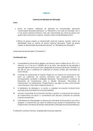
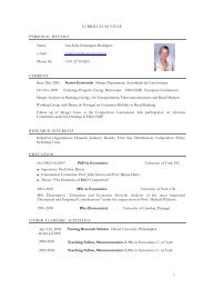
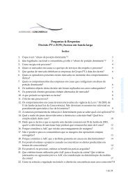
![Versão Pública Nota: Indicam-se entre parêntesis rectos [â¦] as ...](https://img.yumpu.com/39768942/1/184x260/versao-pablica-nota-indicam-se-entre-parantesis-rectos-a-as-.jpg?quality=85)