Nonequilibrium Molecular Dynamics Simulations of Steady-State ...

4204 Ind. Eng. Chem. Res., Vol. 35, No. 11, 1996This flux is defined to give Stefan diffusion (Taylor andKrishna, 1993). For a direct physical interpretation ofthe relative molar flux, also see eq 6. Here J h and J lare given with the surface as the frame of reference.The relative flux, J r h , gives a more convenient chemicalforce as used before (Kjelstrup Ratkje et al., 1995).There is a certain degree of freedom in the choice offluxes and forces. The entropy production rate is, ofcourse, invariant to the choice. With the fluxes givenabove, the thermal force is ∇(1/T), where T is thetemperature, and the chemical force is -∇ T µ h /T, whereµ h is the chemical potential of h. Subscript T meansthat the temperature derivative of the chemical potentialgradient is not taken. It follows from eq 1 that thenumber of independent thermodynamic forces is two.Although the fluxes and forces are vectors, we considerhere only the contributions normal to the interface. Wechoose this normal to be the x direction, which gives ∇) ∂/∂x.The fluxes of heat and mass in the column are linearlyrelated to these forces by∇TJ q )-l qqT - l ∇ T µ h2 qhTJ r ∇Th )-l hqT -l ∇Tµ h2 hhTThe phenomenological coefficients (the l coefficients) areproperties of the system; i.e., their values depend on thesystem’s local intensive thermodynamic variables. Onsager’sreciprocity relation (l hq ) l qh ) was confirmed fora supercritical state by nonequilibrium molecular dynamicssimulations by Hafskjold and Kjelstrup Ratkje(1995) for much larger gradients than found in adistillation column, and we shall assume validity alsoin the present case. When the coupling coefficients l hqand l qh can be neglected, or one of the fluxes is zero, eq3 and 4 can be recast into the form of Fourier’s andFick’s laws (see below).Standard engineering texts uses the assumption ofconstant molal overflow to find the number of theoreticalstages in a McCabe-Thiele diagram (see any textbookin chemical engineering, e.g., Lydersen, 1983). Thisassumption, which means that the number of moles ofliquid entering one stage equals the number of molesof liquid leaving the same stage, implies operating lineswith constant slopes. In eq 2, constant molal overflowmeans J h ) -J l (equimolar counterdiffusion). Theenthalpies of vaporization of the components are takento be almost the same under constant molal overflow(Lydersen, 1983). In the general situation, the enthalpiesare different, and the operating line is bending.Nonequilibrium thermodynamics does not use the assumptionof constant molal overflow a priori, and thepossible bending of the operating line is a consequenceof a significant coupling term in eqs 3 and 4. Nonequilibriumthermodynamics therefore gives a more generaldescription of distillation.The minimum energy needed to separate an isothermalmixture is the Gibbs energy of separation, ∆G,representing a reversible process. The energy neededin excess of the Gibbs energy is the local entropyproduction rate per unit volume, θ, times the absolutetemperature, T, integrated over the column volume, V,and time, t (Kjelstrup Ratkje et al., 1995). The totalwork needed for the separation is then(3)(4)W ) ∆G + ∫ t∫ VTθ dV dt (5)For reversible conditions, θ is zero. This correspondsto the condition of zero thermodynamic loss (Dhole andLinnhoff, 1993). This is a situation of no practicalinterest, because such processes are infinitely slow. Ithas long been known that close to global equilibrium,minimum entropy production occurs at steady states(Prigogine, 1947). In order to obtain a more usefulresult, Tondeur and Kvaalen (1987) proposed that thedistribution of the entropy production rate over theprocess equipment should be uniform. We have shownthat the entropy production rate will be minimum, fora given demand on the output, when the forces of eqs 3and 4 are equipartitioned over the process equipment(Kjelstrup Ratkje et al., 1995; Sauar et al., 1996). Whilespecial knowledge of the phenomenological coefficientsis not necessary for the direct application of the principleof equipartition of forces, such knowledge is useful infinding potential regions of reduction of the entropyproduction. In their attempt to numerically estimatethe entropy production of a distillation column, KjelstrupRatkje et al. (1995) used the assumption ofnegligible entropy production in the liquid phase as wellas on the surface. Other assumptions, which are notgood for actual columns, were constant phenomenologicalcoefficients and area for transfer on each stage. Inthe present work, we do not need such assumptions, aswe calculate the entropy production rate directly frommolecular properties. The results obtained can thereforebe used to discuss the previously used assumptions.Information about fluxes and forces in eqs 3 and 4helps us to quantify the energy efficiency of the columnthrough eq 5. Through the variables and coefficientsof eqs 3 and 4, we know which processes are ratelimiting, and from eq 5, we then know where the energyis required for separation. In this way, eqs 3-5 areimportant for column design and operation: They givethe second law efficiency of the column (through eq 5)and enable the application of the principle of equipartitionof forces.It is very laborious to measure the transport coefficientsfor a gas/liquid interface, the forces, the fluxes,and thus the entropy production rate. This makesnonequilibrium molecular dynamics simulations (NEMD)an attractive tool for the study of such systems. In arecent review (Kjelstrup Ratkje and Hafskjold, 1996),we analyzed some natural and technical processes thatare characterized by transport of heat and mass, interms of NEMD; the basic finding was that the moleculesof the systems distribute in a stationary-statetemperature gradient so as to conduct heat (or mass)in the most effective way. The systems reported includedtransports of heat and mass both in a binary,homogeneous mixture and in a one-component systemundergoing a liquid-vapor phase transition (Ikeshojiand Hafskjold, 1994; Hafskjold and Ikeshoji, 1996).In this article, we continue the work on nonequilibriumthermodynamics and NEMD which are relevantfor distillation. We want to study heat and masstransfer across the liquid/vapor interface and, in particular,spatial variations in entropy production rate,fluxes, and forces. The following questions are ofinterest: What are typical variations in temperatureand composition across an interface, given a temperaturegradient across the system? In Fick’s law ofdiffusion, the concentration gradient is the driving forceof transport. Is this applicable to the system? What

are the conditions for application of Fourier’s law? Thecoupling coefficients are relatively small in bulk materials(Kincaid et al., 1992; Kincaid and Hafskjold, 1994).We shall see that the term containing the couplingcoefficient (i.e., the heat of transfer) cannot be neglectedin the expression for heat fluxes in distillation-likephenomena. How do the entropy production rate andthe conjugate fluxes and forces vary across the interfacein this situation? What are the major contributions tothe entropy production? Can the results support theassumptions in the numerical analysis of distillationcolumns of Sauar and co-workers (1995, 1996)? Whichpractical consequences can be seen from the results? Isthe steady-state situation compatible with uniformdistribution of the entropy production (Tondeur andKvaalen, 1987)?This paper starts with a summary of some conceptsfrom nonequilibrium thermodynamics. We continuewith a short description of the NEMD method beforewe give the results of the simulations. Variations ofintensive variables across the interface, fluxes, andforces for separation of isotope (ideal) mixtures andnonideal mixtures are reported. NEMD simulation dataof these systems also offer the possibility of extractingphenomenological coefficients for the bulk and for thesurface as such, and we shall to some extent discussthe diffusion coefficient and the thermal conductivity.The molecular interpretation of their values, however,is outside the topic of the present paper and will begiven later. Finally, we discuss the local entropyproduction and the application of the results to analysesof distillation.Heat and Mass Transports in a DistillationColumnIn a distillation column, gas is in close contact withliquid, and the main question we address here is howthe interface influences the transport processes. Weconsider a planar interface with infinitely large reservoirsof matter and heat both in the gas and liquidphases. The transport path is chosen from a point inthe bulk gas to a point in the bulk liquid, and wedescribe the exchange of components h (heavy) and l(light) and of heat, between the gas and liquid. Thedriving forces are a temperature gradient and a chemicalpotential gradient, as in eqs 3 and 4. Component l,the component with the lowest boiling point, is enrichedat the top of the distillation column.The relative molar flux of component h is also relatedto its velocity byJ h r ) c h (v h - v l ) (6)where v k is the velocity of component k (k ) h, l) relativeto the interface (dimension m s -1 ) and c h is the molarconcentration of component h (mol m -3 ). There is norseparation when J h ) 0, which makes this flux ameasure of practical interest.The heat of transfer, q*, is defined by the coefficientratio l qh /l hq and byJ q )-λ∇T+q*J hr(7)The heat of transfer refers to the relative flux, J h r ,according to this equation. The thermal conductivityis from eqs 3, 4, and 7:Ind. Eng. Chem. Res., Vol. 35, No. 11, 1996 4205(8)λ ) 1 T 2( l qq - l hq l qhl hh)Fourier’s law for the nonuniform mixture is obtainedwhen the mass flux is zero:(J q ) Jh r)0 )-λ∇T (9)We shall say here that Fourier’s law applies when thethermal conductivity of eq 9 is constant. Fick’s lawdefines the isothermal diffusion coefficient, D:(J h r ) ∇T)0 )-D c x l∇x h (10)where c is the total molar concentration of the mixture.We shall also say that Fick’s law applies when the ratioDc/x l is constant. The D as defined here is exactly thesame as the D in the molar reference velocity (de Grootand Mazur, 1969). For isothermal systems, we havefrom eq 4(J h r ) ∇T)0 )-l hh∇ T µ hTThe isothermal diffusion coefficient, D, is related to thephenomenological coefficient, l hh ,bywhere f h is the activity coefficient of the heavy component,with activities on a mole fraction basis. We noteat this point that all the factors except the thermodynamicfactor, i.e., the parentheses at the right-hand sideof eq 12, are positive. The thermodynamic factor is alsonormally positive (Taylor and Krishna, 1993), but inextreme cases (like for phase splitting), ∂ ln f h /∂ ln x hmay be smaller than -1, with a negative “diffusioncoefficient” as the result. We shall see that localconditions near the vapor/liquid interface for a nonidealmixture is one such case.In the presence of a temperature gradient, the masstransport is described by a combination of eqs 4 and 10:where R hl is the thermal diffusion factor defined by(11)D ) l hh R x lcx h( 1 + ∂ ln f h∂ ln x h)(12)J r h )-D c x l( x h x l R ∇ThlT + ∇x h) (13)R hl )- Tx h x l( ∇x h∇T)Jh )J l )0(14)We shall use constant mass fluxes, J h and J l , in thiswork. The separation flux, J r h , is not constant, however.The total heat flux referring to the wall or theinterface, which here is the enthalpy flux, J H , is relatedto the measurable heat flux byJ H ) J q + H h J h + H l J l (15)where H k is the partial molar enthalpy of component k.Conservation of energy means in the stationary statethat the enthalpy flux is constant throughout thesystem.When we eliminate the chemical force ∇ T µ h /T fromeq 3 by application of (4), the entropy production rate

4206 Ind. Eng. Chem. Res., Vol. 35, No. 11, 1996can be written aseqs 2 and 3. Our results must be understood withinthese contexts.Simulation Method. The MD cell contained 2048particles, 1024 of each type. The cell was noncubic withaspect ratios L x /L y ) L x /L z ) 8(L q is the length of thecell in the q direction), and it had normal periodicboundary conditions.The coupled heat and mass transport was generatedas follows: The cell was divided into 64 layers of equalthickness perpendicular to the x axis. To generate aheat flux, layers 1 and 64 (counting from one end of thebox) were thermostated to a high temperature T H , andlayers 32 and 33 (in the center of the box) werethermostated to a low temperature T L . In this way,there is a heat source at each end of the box and a heatsink in the center. The high-temperature and lowtemperatureregions will be referred to as regions H andL, respectively. This gave a symmetry plane in thecenter of the cell, consistent with periodic boundaryconditions. Periodic boundary conditions are used inthese simulations in order to obtain sufficient accuracyin the simulation of one liquid/vapor interface. Inaddition to giving a heat flux from the warm ends tothe cold center of the cell, the temperature profile alsogenerated a liquid region in the center with one vaporregion at each side. A snapshot of the configuration isshown in Figure 1, where components h and l arerepresented by black and white circles, respectively. Theliquid phase in the center of the cell with vapor at eachside is clearly seen.Mass diffusion was generated by particle swappingfrom type l to type h in region H and simultaneouslyfrom type h to type l in region L. This gave a surplusof type h particles in region H and of type l in region L,with a consequent diffusive mass flux in between.Finally, a mass flux simulating a net transport fromthe vapor to the liquid was generated by moving arandomly chosen particle of type h from region L toregion H, such that the particle maintained its y and zcoordinates, but the x coordinate was shifted by a valueL x /2. The particle insertion into layer H was made witha certain probability given by the Boltzmann factor inorder to avoid large perturbations to the energy of thesystem.Simulation Conditions. The system was a binarymixture of Lennard-Jones/spline particles (Holian andEvans, 1983). Twelve cases were studied as specifiedin Table 1. In all cases, the Lennard-Jones potentialparameters were equal (σ hh ) σ hl ) σ lh ), while the massratios m l /m h were 0.1 and 1 and the parameter ratioɛ ll /ɛ hh was 1.0 or 0.8 (see Table 1). These sets ofparameters mean that we are dealing with an idealisotope mixture in runs 2-7 with m l /m h ) 0.1 and ɛ ll /ɛ hh ) 1.0. This mixture has zero enthalpy of mixing.Nonideality is introduced in runs 8-12 by using m l /m h) 1 and ɛ ll /ɛ hh ) 0.8. The nonideal mixture has a nonzeroenthalpy of mixing and, therefore, an activitycoefficient different from unity.We used T* H ) 1.0, T* L ) 0.7, and the overall numberdensity n* ) Nσ hh 3/V ) 0.4 in all cases. The reducedtemperature is defined as T* ) k B T/ɛ hh where k B isBoltzmann’s constant. The phase diagram of thissystem is to some extent known (Halseid, 1993), andwe chose the overall temperature and density in such away that we got about equal volumes of vapor and liquidin the cell.Calculation conditions and some results from theNEMD simulations are reported in Table 1. All quantiθ) λ (∇TT ) 2 - l hql hhJ hr∇TT 2 + l qhl hhJ hr∇TT + (J r h) 22l hh(16)Two of the terms in eq 16 cancel because l hq ) l qh . Thetotal entropy production rate in the vapor, liquid, andinterface per unit interfacial area is therefore( λ ∇TΘ ) ∫ gl[2T )+ (J r h) 2l hh]where the local entropy production is integrated fromacross the system, from the bulk gas (g) to the bulkliquid (l). The entropy production is positive, in agreementwith the second law of thermodynamics. Equation17 expresses that the energy needed in excess of ∆G(cf. eq 5) increases with increasing superheating of thevapor (∇T) and with increasing separation flux, J r h . Itis reduced by a high mass-transfer coefficient l hh , andalso by a high coupling coefficient, l hq , or heat oftransfer, q*, since in eq 8 the term l hq l qh /l hh reduces theheat conductivity and thereby the entropy productionrate.Equation 17 will be used for a discussion of relativecontributions to the entropy production rate. It differsfrom eq 1 in the way that it gives a clear separationbetween the dissipation by pure heat conduction andby pure mass transfer. In eq 1, the heat flux in the firstterm also contains an effect from the mass flux and viceversa for the mass flux in the second term.It is a problem that the transport coefficients for heatand mass transfer generally are not known. Introductionof average transport coefficients can simplify thesituation. When we consider serial transports, it isappropriate to consider the average resistance to therflux. Since J h is constant across the system, theaverage transport coefficient enters as the coefficientof the second term of eq 17.1) 1 ∫ l dxl ij L gl ij (x)where L is the length of the path. The application ofeq 18 facilitates numerical analyses of eq 17. We shalldiscuss briefly the possibility of finding such averagecoefficients.Molecular Dynamics Simulations of theCoupled Transport of Heat and MassThe basis for our NEMD simulations is describedelsewhere (Ikeshoji and Hafskjold, 1994; Hafskjold etal., 1993; Hafskjold and Kjelstrup Ratkje, 1995), andwe shall only briefly describe the method here. Themain purpose of the simulations is to study how thedifferent variables and derived properties vary acrossthe interface between liquid and vapor. In order toobtain a sufficient statistical accuracy of computedresults, in particular for the vapor phase, we will haveto use temperature and concentration gradients in thesimulations which exceed the real gradients in a columnby several orders of magnitude. Still we shall see thatuseful conclusions can be obtained. The size of thesimulation box is some 35 molecular diameters. Thisis a range which barely extends the interface. It canbe regarded to cover the laminar dissipative films in thebulk vapor and liquid phases, which are described bydx (17)(18)

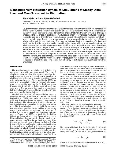
Ind. Eng. Chem. Res., Vol. 35, No. 11, 1996 4207Figure 1. Snapshot of the isotope mixture used in the molecular dynamics simulation. The heavy component is represented by blackcircles, the light component by white circles. In Ar units, the system has a temperature gradient of approximately -4 × 10 9 Km -1 in thegas and approximately -10 8 Km -1 in the liquid. The mole fraction gradient is approximately 10 7 m -1 (case 4, Table 1).Table 1. Simulation Conditions and Results for Enthalpy and Mass Fluxes acomment case m l/m h ɛ ll/ɛ hh z h 10 3 J* H 10 3 J* h ( 10 10 3 J* l ( 10pure heat conduction 1 N/A N/A 1.0 1.64 ( 0.06 N/A N/Aequimolar overflow distillation 2 1.0 1.0 0.5 1.25 ( 0.05 0.31 -0.31thermal diffusion 3 0.1 1.0 0.5 2.3 ( 0.2 0 0equimolar overflow distillation 4 0.1 1.0 0.5 2.2 ( 0.2 0.34 -0.34equimolar overflow distillation 5 0.1 1.0 0.5 1.8 ( 0.2 1.54 -1.54distillation 6 0.1 1.0 0.5 2.4 ( 0.2 0.95 -0.59distillation 7 0.1 1.0 0.5 6.1 ( 0.2 4.06 -1.45thermal diffusion 8 1.0 0.8 0.8 3.31 ( 0.05 0 0equimolar overflow distillation 9 1.0 0.8 0.8 2.60 ( 0.06 0.41 -0.41equimolar overflow distillation 10 1.0 0.8 0.8 2.52 ( 0.08 0.87 -0.87distillation 11 1.0 0.8 0.8 3.34 ( 0.06 0.66 -0.41distillation 12 1.0 0.8 0.8 7.16 ( 0.07 3.12 -0.73a Component mass ratio is m l/m h, Lennard-Jones/spline potential parameters that vary are ɛ ll/ɛ hh ()ɛ lh/ɛ hh), z h is the average molefraction of h in the mixture, J* H is the reduced enthalpy flux, and J* h and J* l are reduced component fluxes. N/A means not applicable.ties are given in reduced Lennard-Jones units, i.e.,reduced enthalpy flux, J* H ) J H (σ 3 hh /ɛ hh )(m h /ɛ hh ) 1/2 , andreduced molar flux, J* i ) J i (σ hh 3M h /m h )(m h /ɛ hh ) 1/2 , whereM h is the molar mass of h. The details of the calculationof the temperature (from the equipartition principle),the fluxes, and the forces were given before (Hafskjoldet al., 1993). The entropy production rate was calculatedfrom eq 1.Case 1 of the NEMD simulations is a case of pure heatconduction for the single component h. The heat flux,J q , is constant across the interface. Cases 2-7 representideal mixtures, while cases 8-12 are for nonidealmixtures; see Table 1.In cases 2, 4, 5, 9, and 10, we used J l )-J h to studythe assumption of constant molal overflow. These caseshave contributions to J q from both heat and masstransfer. For the ideal mixture, the heat of vaporizationof component l exactly cancels the heat of condensationof component h.Cases 3 and 8 represent pure heat conduction in ideal(case 3) or nonideal (case 8) mixtures. Cases 6, 7, 11,and 12 represent combinations of intermolecular diffusion,condensation, and evaporation. These are thecases that model distillation in general, as componenth condensates and l evaporates.Results and DiscussionThe results for the density, composition, and temperatureas a function of distance x are given in Figures 2,3, and 4. Figure 3 gives the separation of mass for thetemperature gradients of Figure 4. The heat flux andthe relative mass flux are given in Figures 5 and 6,while the entropy production rate is shown in Figures7 and 8 for cases 1-8 and for a homogeneous binarymixture, respectively. All results are given in dimensionlessvariables is these figures.Numerical Results for an Ar-like Isotope Mixture.The results reported in this work can be usedwith any mixture for which the molecular diameter, σ,the mass of the heavy component, m h , and the Lennard-Jones potential energy depth, ɛ/k B , are known. For thesake of getting some numerical insight, we shall use anideal mixture with mass ratio m l /m h ) 0.1. For Ar-likeparticles, we then have the diameter 3.405 Å, the mass6.64 × 10 -26 kg, and ɛ/k B ) 120 K. (The resultingseparation has no practical interest.) The averagetemperature gradients over the system are then enormous,-4 × 10 9 Km -1 in the vapor and -10 8 Km -1 inthe liquid. These gradients are very large compared togradients one can achieve in the laboratory. We havestudied earlier such gradients and established by NEMD(Hafskjold and Kjelstrup Ratkje, 1995) that the basicassumption of nonequilibrium thermodynamics, that oflocal equilibrium, is still valid.We get an order-of-magnitude estimate for the dissipatedenergy by separating an equimolar mixture ofhandlin∆t)1s,forA)1m 2 transfer area byintegrating the equation, using estimates of the averagevalues for T and θ:Θ ≈ TθA∆x∆t (19)Here ∆x is the distance needed to achieve pure componentsin the actual composition gradient. We choosethe reduced variables m* ) 1, T* ) 1, n* ) 0.4, J* h )10 -3 , J* H ) 10 -3 , and θ* ) 10 -4 , which correspondroughly to case 5. Using Ar as an example, we thenget T ) 120 K, n ) 16 800 mol m -3 , J h ) 6650 mol m -2s -1 , J H ) 6.7 × 10 6 Jm -2 s -1 , and θ ) 1.6 × 10 13 JK -1m -3 s -1 . The mole fraction gradient read from Figure3 for case 5 converted to Ar units gives that ∆x ) 1.8 ×10 -8 m is needed for full separation. This gives the totaldissipated energy equal to 35 × 10 6 J (for 6650 mol).For comparison, the Gibbs energy of demixing theequimolar mixture into pure components under thesame conditions is 9 × 10 6 J. The total work needed toperform the separation is the sum of the two, 44 × 10 6J, leading to a second law efficiency for the separationof 20% (eq 5). This efficiency is not realistic for severalreasons. Firstly, it assumes that separation takes placein one step. Secondly, it assumes that products are

Ind. Eng. Chem. Res., Vol. 35, No. 11, 1996 4209Figure 5. Variation in the heat flux across the interface for someselected ideal (white symbols) and nonideal (black symbols)mixtures.Figure 4. Temperature profiles across the vapor/liquid interfacein the stationary states given in Table 1.used with constant Dc/x l also across the interface. Thiscannot be done for cases 5 and 7, where the diffusivefluxes are larger and Dc/x l jumps at the surface. Thedifference between cases 4 and 5 is noteworthy sincethese cases model similar situations: equimolar diffusion.It is the difference in molar flux that gives thedifference in mole fraction profiles between cases 4 and5, as the heat flux is very similar in the two cases (seeTable 1).The nonideal mixtures have a region near the interfacewhere diffusion occurs against the compositiongradient. The consequence is that the mutual diffusioncoefficient, as defined locally by Fick’s law, is negativein this region, cf. eq 10. The transport is, however,along with the chemical potential gradient. The transportis also along the temperature gradient. The processis therefore not in disagreement with the second law ofthermodynamics. The importance of using forces for thetransports given by nonequilibrium thermodynamics isemphasized by this finding.We conclude that the product Dc/x l in Fick’s law isconstant in bulk mixtures of ideal liquids and gases. Atthe interface, there may be a jump in this variable. Theproduct may be taken as constant for bulk nonideal gasFigure 6. Relative molar flux across the interface for someselected ideal (white symbols) and nonideal (black symbols)mixtures.and liquid mixtures only with great care. Fick’s lawfails in the surface region of the these mixtures.The temperature profiles for all cases studied areshown in Figure 4. All cases have a linear temperatureprofile in the liquid phase, which means that the heatconductivity of Fourier’s law is constant in this phase.The relatively small temperature gradients in the liquidphase mean that the heat conductivity is larger for thisphase than for the vapor. Cases 1, 3, and 8 were usedto compute the thermal conductivity. A significantincrease from gas to liquid and a smooth variation

4210 Ind. Eng. Chem. Res., Vol. 35, No. 11, 1996Figure 7. Entropy production rate for heat and mass transportacross an interface with ideal (white symbols) and nonideal (blacksymbols) mixtures.vapor interface. This has support in kinetic theory(Ytrehus and Østmo, 1996) and molecular dynamicssimulations (Yasuoka et al., 1995). Different kineticenergies are then associated with the condensing andevaporating molecules, and these energies must havean impact on the steady-state distribution of mass inthe temperature gradient (the Soret equilibrium), cases3 and 8 (Hafskjold et al., 1993).We know that the Soret effect can be neglected in thevapor phase and gives a 10% contribution from the firstterm of eq 13 in the liquid phase (Kincaid et al., 1992;Kincaid and Hafskjold, 1994). At the surface, the Soreteffect is as yet unknown. We have seen that thepresence of an interface has an impact on the temperatureprofile in the gas phase. It therefore appears thata bigger value can be expected at the interface than inthe bulk phases. We predict a big value from eq 24below.Heat Flux across the Phase Boundary. The heatfluxes for selected cases are shown in Figure 5. Thegeneral picture is that the heat flux is close to constantin the bulk phases, but in cases with a source term atthe interface (the heat of condensation), it changessharply at the interface, i.e. the coupling coefficients ofeqs 3 and 4 are significant. This is illustrated by case7, in which there is a net condensation of vapor (|J h | >|J l |). In cases 1, 3, and 8, J q is constant because J l ) J h) 0. In case 5, J q is constant because J l )-J h and thetwo components have the same heat of vaporization.Equation 15 explains why the measurable heat flux,J q , is generally not constant throughout the system.Generally, the last terms contribute. Neglecting thecontributions from the heat of mixing, we may rewritethe heat flux of eq 15:J ql) J q v + ∆ vap H l J l + ∆ vap H h J h (20)where superscripts l and v represent liquid and vapor,respectively, and ∆ vap represents a change upon vaporization.Depending on the relative magnitude of thefluxes, the first or the last two terms on the right-handside of eq 20 may be small compared to the other terms.For small temperature gradients, it may be useful toassume that the heat flux in the liquid phase is givenby the net heat effect of condensation and evaporation,i.e., the last two terms of eq 20. This means that wecan writeFigure 8. Entropy production rate for heat and mass transportin an ideal homogeneous mixture.across the interface was found (not shown here). Fourier’slaw can then be applied locally only when theposition dependency of the heat conductivity is known.The most interesting feature of the stationary-statetemperature profile in the gas phase and through theinterface is its nonlinearity near the interface. Thenonlinear part near x/L x ) 0 is a “wall” effect of the Hlayers due to the thermostat and low density, but theshoulder that shows in most profiles is due to propertiesof the gas-liquid system. It should be noted that eventhe simple cases of heat conduction only (cases 1, 3, and8) show the shoulder in the temperature profile. Theposition of the shoulder is clearly on the gas side of theinterface. An independent simulation of a single-phasevapor mixture subject to the same temperature differencedid not give this shoulder. We conclude that theshoulder is a consequence of heat effects at the liquid/J ql≈ ∆ vap H l J l + ∆ vap H h J h (21)These terms will sum to a constant when the massfluxes are constant. Constant mass fluxes were usedthroughout these simulations, meaning that the approximation(21) is valid only for case 7 in Figure 5. Inlthe other cases of this figure, we have J q ) J v q .The pure heat conductance term (the first term onthe right-hand side of eq 20 since the thermal diffusionfactor is small) is of the order 2-3 × 10 -3 in Lennard-Jones units as taken from Figure 5. Although thescatter of the data is higher in the liquid than in thelvapor, J q is of the same order in all the cases shownexcept case 7, where it is approximately 13 × 10 -3 .Incase 7, there is a net mass flux from the vapor to theliquid, which means that there is a significant heatsource due to condensation at the interface (see eqs 7and 20). Even though there is also a diffusive mass fluxin case 5, it does not give a heat source since the heatof condensation of component h exactly cancels the heat

of vaporization of component l in the isotope mixture.Cases 1, 3, and 8 are cases of pure heat conduction insystems without net mass flux.The approximation (21) is not generally true forcondensation or distillation. Equimolar diffusion of thecomponents in ideal mixtures gives no heat sink orsource at the interface, and then the terms of eq 21cancel, and vice versa, equimolar diffusion need not bemaintained when the enthalpies of vaporization aredifferent as in case 9 or 10. This result is in agreementwith the conclusion reached long ago by Krishna (1977)from analysis of multicomponent distillation.Nonequilibrium thermodynamics gives, for these reasons,a more accurate description of distillation than theequilibrium stage model. From knowledge of the heatof transfer, one may calculate the impact of the massflux on the heat flux in eq 7. This will further determinethe mass or volume of the bulk streams in a distillationcolumn, the operating line, and the number of theoreticalstages.Relative Mass Flux across the Interface. Therelative mass flux, J r h , is shown in Figure 6. We see asystematic difference between the fluxes for ideal andnonideal mixtures. The ideal mixtures, cases 4-6, arenot associated with a large change in composition acrossrthe interface, and J h is monotonous. The nonidealmixtures, cases 9-12, show an interesting feature:There are extremal values for J r h at the interface.A minimum in J r h represents a tendency to collectivemotion of the two components, whereas a maximum inJ rh indicates a strong tendency for separation at theinterface, cf. eq 6, in accordance with ∂ ln f h /∂ ln x h beingnegative in eq 12. When the thermodynamic drivingforce, ∇ T µ h /T, is monotonous across the interface, thephenomenological coefficient, l hh , has a a maximum atthe interface and a minimum just outside (on the vaporside). Physically, this means that the rate-limiting stepfor mass transfer is in the vapor. The explanation forthe maximum at the interface is that the equilibriumcompositions favor a higher concentration of h in theliquid than in the vapor and vice versa for component l(see Figure 2). Since fluxes J h and J l are constant acrossrthe interface, the maximum in J h is a direct consequenceof the mole fraction ratio x h /x l in eq 2. Althoughthere is probably no anomaly in the thermodynamicdriving force, the equilibrium compositions are such thatseparation is enhanced at the interface. The minimumrin J h is more subtle, although it may simply be aconsequence of the maximum discussed above, superimposedon the sloping curves we also see for the idealmixtures. The apparent collective motion may, however,also be a separate phenomenon near the interfaceand, like the shoulder in the temperature profile shownin Figure 4, be related to the escape/capture processbetween the vapor and the liquid.The relative mass fluxes for cases 2, 4, and 6 show asmaller change in J r h at the interface. The fluxes arealso relatively small. Considering the large gradientsthat we apply in the simulation, we may expect a nearlyconstant value in practical situations for such idealmixtures.Heat of Transfer. One procedure to find the heatof transfer can be obtained by combining eqs 7 and 20,which gives for the liquid phaseInd. Eng. Chem. Res., Vol. 35, No. 11, 1996 4211should be reasonably good. For ideal mixtures with∆ vap H h ≈ ∆ vap H l , we than see that q* vanishes at theinterface. This explains why the interface has such asmall impact on the separation of isotopes, cf. upper partof Figure 3. The heat of transfer can always be expectedto be significant at the interface for nonideal mixturedistillation, as exemplified by cases 9, 10, and 6.rThe value of J h differs from stage to stage in adistillation column, depending on the driving forces forseparation at the stage in question. This means thatq* probably varies across the column. The heat oftransfer may be positive or negative depending on therelative magnitude of the two heats of vaporization ineq 22. This has an impact on the action of the forces ofeqs 3 and 4. The forces may enhance or counteract eachother, depending on the sign of q*. A positive thermalforce reduces J r h when q* is negative. A positive valuefor the heat of transfer is beneficial when a large valuefor J hr is wanted.Entropy Production Rate. The local entropy productionrate from the thermal flux and force and themass separation flux and force was calculated accordingto eq 1 and shown in Figure 7.The first conclusion to be drawn from this is that theentropy production rate of the surface may be significantcompared to the entropy production rates in layers ofsimilar thickness in the adjoining bulk phases. It is onlywhen the mass fluxes are at the largest (case 7) thatthe entropy production rate in the liquid becomes muchlarger than that of the surface. Otherwise, the valuesare comparable in magnitude. We expect that this willhold also for smaller (real) gradients. All parts of theentropy production rate therefore play a role in theexcess energy needed in terms of ∆G in eq 5. This fitswith practical experience. It is hard to make a clearcutassignment of the phase which is rate limiting forcolumn performance.The contribution from the thermal flux and force tothe entropy production rate is generally smaller thanthe contribution from the chemical flux and force, andit is negligible in the liquid. However, the peak nearthe interface is dominated by the thermal contribution(not shown) and can account for as much as one-thirdof the total entropy production rate in the vapor (Hafq*) J v q + ∆ vap H l J l + ∆ vap H h J h + (λ∇T) lrJ hwhere superscripts v and l represent vapor and liquid,respectively. For equimolar overflow, J l )-J h , thisexpression reduces toq* ) J v q + (λ∇T) l+ (∆rvap H h - ∆ vap H l ) J hrJ h J h(22)(23)We found from Figure 5 that the measurable heat fluxfor the ideal mixtures was rather independent of themass fluxes in the gas phase for equimolar flow andconstant across the interface. This implies that J q v ≈-λ∇T, and the numerator in the first term on the righthandside of eq 23 vanishes. In such cases, the modelq* ≈ (∆ vap H h - ∆ vap H l ) J hJ hr ≈constant(∆ vap H h - ∆ vap H l ) (24)

4212 Ind. Eng. Chem. Res., Vol. 35, No. 11, 1996skjold and Kjelstrup Ratkje, 1996). The entropy productionrate is of the same order of magnitude in theliquid and vapor. These results do not support theassumptions made by Kjelstrup Ratkje et al. (1995) intheir estimation of the entropy production rate, viz.neglecting the thermal contribution to the entropyproduction and the entropy production in the liquidphase. We see that NEMD can be used to give the localvalue of the entropy production rate.Comparison of eqs 1 and 17 gives that, if l hq ) l qh >0 (usually the case), it is better to neglect the “thermalcontribution” to the entropy production rate in eq 17than in eq 1. In eq 17, the two terms proportional tothe coupling terms in eq 16 cancel. The finite value ofthe coupling term reduces the thermal contribution (cf.eq 16) and increases the contribution from the massflux. For the same reason, it is better to neglect thecontribution from the mass flux in eq 1 than in eq 17.The two forms therefore serve different purposes.The striking feature of Figure 7 is that all simulationsperformed even for the one-component system show amaximum in the entropy production rate slightly at thevapor side of the interface. The maxima are larger forcases which have a nonnegligible q*.By contrast, the entropy production rate in a homogeneousideal two-component mixture shows a monotonousincrease from the hot to the cold side (Figure 8).The entropy production rate is not uniformly distributedin the stationary state, neither in the one-componentsystem nor in the two-component system.The results also show that forces are generally notconstant across the interface. The concentration gradientsin the liquid and gas ideal mixtures are constant(Figure 3). The temperature gradients are constant onlyin the liquid phase (Figure 4) (for both ideal andnonideal mixtures). Consequently, the definition of anaverage diffusion coefficient for transport across theinterface (eq 18) is easy for ideal mixtures; otherwise,the definition is nontrivial in the sense that the integrandin eq 18 may change abruptly across the interface.More work is needed to find such average coefficients.We have previously studied molecular mechanismsof transport of heat and mass in one-phase systems inthe stationary state (Hafskjold et al., 1993; Hafskjoldand Kjelstrup Ratkje, 1995). The heat was most effectivelyconducted in this state by a distribution of thecomponents which gave a constant-concentration gradientin a constant-temperature gradient. When a liquidgastransition is involved, it is clear from Figure 3 thateffective heat transfer does not imply such a simpledistribution. We intend to examine how the systemresponds most effectively to given boundary conditionson a molecular level in a future work.Liquid/Vapor Surface. This study has shown thatthe surface has special transport properties and that itis necessary to use nonequilibrium thermodynamics inthe description of transport in this region. A largerportion of the energy dissipated in the system isdissipated at the surface. (This part of the dissipationis probably unavoidable in the distillation column.)The special properties of the surface region indicatethat the surface can be regarded as a separate systemin the thermodynamic sense, a topic we shall elaborateon in a future article. It is possible to compute allvariables of Figures 2-8 in a well-defined manner alsoin the surface region. The length scale for our investigationis a molecular one (in nanometer), not a macroscopicscale (in micrometers). A formulation of thetransport problem on a micrometer scale can be obtainedby integration over the surface variables; seeBedeaux et al. (1992). Albano et al. (1979) showed thatthe dynamic behavior of the interfacial densities can begiven in terms of interfacial fluxes and extrapolatedbulk densities and fluxes alone. The description isequivalent to a description which uses densities andfluxes which are singular at the surface. The intriguingshoulder of the temperature profile (Figure 4) is anindication that singularities may occur in such a macroscopicdescription.Applications to Distillation. The present work isan attempt to encourage work on nonequilibrium thermodynamicmodeling of distillation. We have shownhow forces and fluxes during distillation of binarymixtures can be defined locally and how they can beincluded into an efficiency calculation of the process.Severe gradients have been applied in the study, butthis means that the general conclusions can be transferredwith certainty to less severe situations. Nonequilibriummolecular dynamics simulation yields valuesfor transport coefficients under conditions that arehardly accessible in practice. The fact that transportdata for the complex transport equations (3 and 4) areavailable through computer simulations may facilitatethe application of nonequilibrium modeling of distillationcolumns. The coefficients obtainable from thepresent data and their molecular interpretation will bediscussed in a further work.In our simulation technique, we set the condition ofequimolar overflow in the computer experiment andinvestigated its consequences (cases 2, 4, 5, 9, and 10).In the real case, the situation is different: The heatsupply to the column is controlled (adiabatic column),and separation follows. When we see a net heat effectat the surface in our simulations, we know that the lastterm of eq 7 plays a role. This is compatible with abending operating line. The sign of the heat of transferwill relate to the curvature of the operating line. Apositive value for q* means that the heavy componenthas a higher flux than the light component (cf. eq 13).The volume of the vapor phase may be reduced, and theoperating line in the rectifying section, say, will increaseits slope. It should be possible to find a revised numberof theoretical stages needed from this information.We have found that average phenomenological coefficients(eq 18) can be calculated by integrating acrosseach of the phases in the ideal system. The assumptionof a negligible contribution to the entropy productionrate from the liquid phase (Kjelstrup Ratkje et al., 1995)was not substantiated from these data, however. Thepresent results mean that the entropy production rateof distillation may depend on the transport propertiesof the surface. This means that it will be important tofind transport coefficients for the surface.Conclusions and PerspectivesThe present work is an attempt to get direct informationon the relationship between the molecular andmacroscopic heat- and mass-transfer properties at thegas/liquid interface. We have seen that the ordinaryFick’s and Fourier’s laws can be used for the liquid andgas separately. As soon as the mixture is not ideal, thethermodynamic equations of transport are needed, andthe properties of the liquid-vapor interface have to betaken into account.On a molecular (nanometer) scale, the intensivevariables of the system are smooth functions across the

interface. There are, however, indications of an anomalyin the temperature profile (a shoulder). Nonequilibriumthermodynamics for surfaces may therefore give adiscontinuity in the temperature at a macroscopic scale.More work is needed to establish the boundary conditionsfor integrations across the surface in this case.The entropy production rate has a peak near theinterface in all the cases we have studied in this work.This peak stems from the shoulder in the temperatureprofile. In the cases studied, the entropy production isof the same order of magnitude in the gas and liquid.The thermal and mass-transfer contributions to theentropy production are also comparable in magnitude.We have indicated how the equations of transportgiven by nonequilibrium thermodynamics can be usedto analyze the efficiency of column elements and calculateoperating lines. The burden of getting transportcoefficients can probably also be eased by applicationof nonequilibrium molecular dynamics simulation techniques.AcknowledgmentB.H. thanks the Agency of Industrial Science andTechnology (AIST) and TRU at the University of Oslofor providing computer resources for this work. B.H.is also grateful to AIST for financial support during hissabbatical stay there.Literature CitedAlbano, A. M.; Bedeaux,D.; Vlieger, J. On the Description ofInterfacial Properties Using Singular Densities and Currentsat a Dividing Surface, Phys. A 1979, 99, 293.Bedeaux, D.; Hermans, L. J. F.; Ytrehus, T. Slow Evaporation andCondensation. Phys. A 1990, 169, 263.Bedeaux, D.; Smit, J. A. M.; Hermans, L. J. F.; Ytrehus, T. SlowEvaporation and Condensation. II. A Dilute Mixture. Phys. A1992, 182, 388.de Groot, S. R.; Mazur, P. Non-Equilibrium Thermodynamics;North-Holland: Amsterdam, 1961; Dover: New York, 1985.Dhole, V. R.; Linnhoff, B. Distillation Column Targets. Comput.Chem. Eng. 1993, 17, 549.Dysthe, D. K.; Hafskjold, B.; Breer, J.; Cejka, D. An interferometrictechnique for measuring interdiffusion at high pressures. J.Phys. Chem. 1995, 99, 11230.Førland, K. S.; Førland, T.; Kjelstrup Ratkje, S. IrreversibleThermodynamics. Theory and Applications; John Wiley &Sons: Chichester, 1988; 2. Reprinted 1994.Hafskjold, B.; Ikeshoji, T. Partial specific quantities computed bynonequilibrium molecular dynamics. Fluid Phase Equilib. 1995,104, 173.Hafskjold, B.; Ikeshoji, T. Non-equilibrium molecular dynamicssimulation of coupled heat- and mass transport across a liquid/vapor interface. Molec. Simul. 1996, in press.Hafskjold, B.; Kjelstrup Ratkje, S. Criteria for local equilibriumin a system with transport of heat and mass. J. Stat. Phys. 1995,78, 463.Hafskjold, B.; Kjelstrup Ratkje, S. Molecular Interpretation ofcouples transport of heat- and mass transport across a vapor/liquid interface. In ECOS’96 Symposium Proceed; Alvfors, P.,Eidensten, L., Svedberg, G., Yan, J., Eds.; Dept. of Chem. Eng.,Royal Insitute of Technology: Stockholm, 1996; p 405.Ind. Eng. Chem. Res., Vol. 35, No. 11, 1996 4213Hafskjold, B.; Ikeshoji, T.; Kjelstrup Ratkje, S. On the molecularmechanism of thermal diffusion in liquids. Molec. Phys. 1993,80, 1389.Halseid, R. The Critical Point of the Lennard-Jones Spline Fluid,Project Report, Norw. Inst. of Technology, Trondheim, 1993.Holian, B. L.; Evans, D. J. Shear Viscosities away from the MeltingLine: A Comparison of Equilibrium and Nonequilibrium MolecularDynamics. J. Chem. Phys. 1983, 78, 5147.Ikeshoji, T.; Hafskjold, B. Non-equilibrium Molecular DynamicsCalculation of Heat Conduction in Liquid and through Liquid-Gas Interface. Molec. Phys. 1994, 81, 251.Kincaid J. M.; Hafskjold, B. Thermal Diffusion Factors for theLennard-Jones/spline System, Molec. Phys. 1994, 82, 1099.Kincaid, J. M.; Li, X.; Hafskjold, B. Nonequilibrium MolecularDynamics Calculation of the Thermal Diffusion Factor. FluidPhase Equilib. 1992, 76, 113.Kjelstrup Ratkje, S.; Hafskjold, B. Coupled Transports of Heat andMass. Theory and Applications. In Entropy and EntropyGeneration: Fundamentals and Applications; Shiner, J., Ed.;Kluwer: Dordrecht, 1996, in press.Kjelstrup Ratkje, S.; Sauar, E.; Hansen, E. M.; Lien, K. M.;Hafskjold, B. Analysis of Entropy Production Rates for Designof Distillation Columns. Ind. Eng. Chem. Res. 1995, 34, 3001.Krishna R. A film model analysis of non-equimolar distillation ofmulticomponent mixtures. Chem. Eng. Sci. 1977, 32, 1197.Linnhof, B.; Townsen, D. W.; Boland, D.; Hewitt, G. F.; Thomas,B. E. A.; Guy, A. R.; Marsland, R. H. User Guide on ProcessIntegration for the Efficient Use of Energy. The Institution ofChemical Engineers; Warks, 1982.Lydersen, A. Mass Transfer in Engineering Practice, Wiley:Chichester, 1983.Prigogine, I. Etude thermodynamique des phenomenes irreversibles.Thesis, Desoer, Liège, 1947.Sauar, E.; Kjelstrup Ratkje, S.; Lien, K. M. Process optimizationby equipartition of forces. Applications to distillation columns.In ECOS’95 Symp. Proceed; Gogus, Y. A., Ozturk, A., Tsatsaronis,G., Eds.; Turkish Soc. for Thermal Sciences and Technology,Mechanical Eng. Dept., Ankara and ASME: New York,1995; Vol. I, p 413.Sauar, E.; Kjelstrup Ratkje, S.; Lien, K. M. Equipartition offorcessa new principle for process design and optimization. Ind.Eng. Chem. Res. 1996, in press.Sigmund, P. M. Prediction of molecular diffusion ar reservoirconditions. Part I. measurement and prediction of binary densegas diffusion coefficients. J. Can. Petrol. Technol. 1976, April-June, 48.Taylor, R.; Krishna, R. Multicomponent Mass Transfer; John Wiley& Sons: New York, 1993.Taylor, R.; Lucia, A. Modeling and Analysis of Multi-componentSeparation Processes. AIChE Symp. Ser. 1995, 91 (304), 19.Tondeur, D.; Kvaalen, E. Equipartition of Entropy Production. AnOptimality Criterion for Transfer and Separation Processes.Ind. Eng. Chem. Res. 1987, 26, 50.Yasuoka, K.; Matsumoto, M.; Kataoka, Y. Molecular Simulationof Evaporation and Condensation I. Self Condensation andMolecular Exchange. In ASME/JSME Thermal EngineeringProceed.; Fletcher, L. S., Aihara, T., Eds.; The American Societyof Mechanical Engineers: New York, 1995Ytrehus, T; Østmo, S. Kinetic Approach to Interphase Processes.Int. J. Multiphase Flow 1996, 22, 133.Received for review April 8, 1996Revised manuscript received August 23, 1996Accepted August 29, 1996 XXAbstract published in Advance ACS Abstracts, October 15,1996.