Mixed Gaussian Process and State-Space Approach for Fatigue ...

More documents

Recommendations

Info

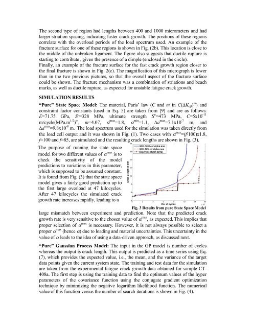
The second type of region had lengths between 400 and 1000 micrometers and hadlarger striation spacing, indicating faster crack growth. The positions of these regionscorrelate with the overload periods of the load spectrum used. An example of thefracture surface for one of these regions is shown in Fig. (2b). This location is close tothe middle of the unbroken ligament. The figure also suggests that ductile rupture isstarting to contribute , given the presence of a dimple (enclosed in the circle).Finally, an example of the fracture surface for the fast crack growth region closer tothe final fracture is shown in Fig. 2(c). The magnification of this micrograph is lowerthan in the two previous pictures, so that the overall aspect of the fracture surfacecould be shown. The fracture mechanism was a combination of striations and beachmarks, as well as ductile rupture, as expected for unstable fatigue crack growth.SIMULATION RESULTS“Pure” State Space Model: The material, Paris’ law (C and m in C(∆K eff ) m ) andconstraint factor constants (used in Eq. 5) are taken from [9] and are as follows:E=71.75 GPa, S y =328 MPa, ultimate strength S u =473 MPa, C=5x10 -11m/cycle(MPa.m 1/2 ) m , m=4.07, max =1.8, min =1.1, ∆a max =7.1x10 -7 m, and∆a max =9.8x10 -8 m. The load spectrum used for the simulation was taken directly fromthe load cell output and it was shown in Fig. (1). Two cases with max =(f/100)x1.8,f=100 and f=85, are simulated and the resulting crack lengths are shown in Fig. (3).The purpose of running the state spacemaxmodel for two different values of is tocheck the sensitivity of the modelpredictions to variations in this parameter,which is supposed to be assumed constant.It is found from Fig. (3) that the state spacemodel gives a fairly good prediction up tothe first large overload at 47 kilocycles.After 47 kilocycles the simulated crackgrowth rate increases rapidly, leading to aFig. 3 Results from pure State Space Modellarge mismatch between experiment and prediction. Note that the predicted crackgrowth rate is very sensitive to the chosen value of max , as expected. This implies thatproper selection of max is necessary. However, it is not always possible to select aproper max (hence ) due to loading and material uncertainties. This uncertainty in thevalue of leads to the idea of using a data-driven approach, as discussed next.“Pure” Gaussian Process Model: The input in the GP model is number of cycleswhereas the output is crack length. This output is predicted as a time series using Eq.(7), which provides the expected value, i.e., the mean, and the variance of the targetdata points given the current system state. The training and test data for the simulationare taken from the experimental fatigue crack growth data obtained for sample CT-408a. The first step is using the training data to find the optimum values of the hyperparameters of the covariance function using the conjugate gradient optimizationtechnique by minimizing the negative logarithm likelihood function. The numericalvalue of this function versus the number of search iterations is shown in Fig. (4).
It is evident that the function convergesto its lowest value, which in turn leads toa prediction of the optimal set of hyperparameters. These hyper parameterswere used to predict the crack lengthsfor two different cases: in the first casethe training data are taken from the first14 experimental points, i.e., up to 80kilocycles (refer to Fig. 5) andcontinuous crack growth data arepredicted from 80 to 170 kilocycles.Fig. 4. Optimization of the function L.In the second case the full set of 32 experimental points are used as the training datato predict a smooth crack growth curve between 40 to 170 kilocycles. Thecorresponding expected values and their 3σ confidence intervals are plotted in Fig. 5.Fig. 5 Simulated crack growth from the “pure” GP modelFrom this figure it can be seen that as the number of training points increases theprocedure provides a better 3σ confidence interval. However, note from Fig. 5b thateven though the test data are available for the whole domain of interest, the GP modelis unable to retain the shape of the measured crack growth curve. This is because ofthe lack of physical information in the Gaussian process model, which results in asmooth “curve fit” of the data. This suggests that a “hybrid” physics and data-drivenapproach should be used. Results for this case are discussed in the next subsection.Hybrid SS-GP (State Space and Gaussian Process) Model: for the hybrid approachsuggested above, the input crack length a k in Eq. (5) is being constantly supplied froma GP data driven model rather than from an error accumulating state space model.Once k is calculated, the future crack length a k is recalculated using the state-spacemodel and the process continues in a loop for the fatigue cycles of interest. Thetraining of the GP model is performed with the full set of experimental points fromsample CT-408a, whereas the validation of the hybrid model prediction is done againstthe experimental data from sample CT-407a. Note that the case of max =1.8 isconsidered. The crack growth rate is shown in Fig. (6) and it is evident that the hybridmodel results in better prediction than those of the state-space model whilereproducing the shape of the experimental crack growth curve fairly well.
Page 1 and 2: Mixed Gaussian Process and State-Sp
Page 3 and 4: a k h(K eff k) with h(0) 0effK k a
Page 5: E647-93 with a width of 25.4 mm (fr

Mixed Gaussian Process and State-Space Approach for Fatigue ...

Create successful ePaper yourself

Delete template?

Save as template?