Mixed Gaussian Process and State-Space Approach for Fatigue ...

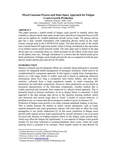
Mixed Gaussian Process and State-Space Approach for FatigueCrack Growth PredictionSubhasish. Mohanty 1 , Rikki. Teale 2Aditi. Chattopadhyay 3 , Pedro. Peralta 4 and Christina Willhauck 5Department of Mechanical and Aerospace Engineering,Arizona State University, Tempe, AZ 85287ABSTRACTThis paper presents a hybrid model of fatigue crack growth in metallic alloys thatcombines a physics-based state-space model and a data-driven Gaussian Process (GP)and can be applied for variable-amplitude aircraft service loads. The physics drivenpart has a state variable formulation with underlying physics based on the crackclosure concept used in the FASTRAN-II model. The data driven part of the modeluses a kernel based GP regression model, which is being considered as the equivalentof an infinite neuron neural network model. The state space part is linked to the datadriven part via a constraint factor k , which accounts for the effects of the stress stateon the plastic-zone size. Through simulations it is shown that the hybrid model givesbetter predictions of fatigue crack length and growth rate as compared to both the purephysics model and the pure data driven GP model.INTRODUCTIONIntensive research and development efforts are currently being dedicated to on-boardsystems for integrated health management of aerospace structures, which need to becomplemented by a prognosis approach. In this regard, a simple form of prognostics,known as a life usage model, is widely used and is based on gathering statisticalinformation about how long a component lasts before failure, and uses thesestatistics, collected from a large population sample, to make remaining lifepredictions for individual components. However, these predictions are not based onmeasured characteristics of the individual components. Another method that iswidely practiced and constantly been improved is a physics based approach. This isprimarily based on fracture mechanics, as far as fatigue failure is concerned. A thirdapproach is the data mining, data driven or the machine learning method, whichuses historical and current usage data to “learn” a model of system behavior. Adetailed review on various data driven prognosis models is given in reference [1].Prediction of fatigue crack growth, even under constant amplitude loading, is not easy.This is mainly because the manner in which various parameters, such as loads,material properties and crack geometries, interact with each other to affect the crackpropagation is not clearly understood [2]. In this sense, prediction of fatigue crackgrowth under typical service loads experienced by aircraft structures is an even moreinvolved task because of loading transient effects in the fatigue crack growth rates,which may affect the fatigue life significantly. A vast majority of fatigue crack growthmodels [3], has been restricted to constant-amplitude stress cycles, where the crackopening stress is assumed to be constant. These models cannot be used directly for1 Graduate Research Associate, Subhasish.Mohanty@asu.edu2 Graduate Research Assistant, Rikki.Teale@asu.edu3 Professor, Fellow AIAA, ASME, aditi@asu.edu4 Associate Professor, pperalta@asu.edu5 Graduate Research Assistant, Christina.Willhauck@asu.edu

variable-amplitude service loading, because they cannot capture the intrinsic dynamicbehavior. The FASTRAN-II [4-6] and the AFGROW [7] models capture thedynamics under variable amplitude by incorporating the crack opening stress as aphysical variable in the fatigue crack growth model. Under variable-amplitudeloading, these models typically rely on a memory-dependent variable (e.g., crackopening stress) that requires knowing the load history. In general the model is moreaccurate if the load history is considered, but that is not always the case. Accountingfor the load history makes a model more complicated and time-consuming forcalculations, and load histories are not always available. It would be beneficial toestablish a procedure whereby load history is not explicitly required but is accountedfor in other ways, such as an additional equation for an extra (state) variable withmemory, which would likely make the model more computationally efficient. Thestate space model presented in [8-11], though based on the original physical concept ofthe FASTRAN model [4-6], significantly reduces the computation time and memoryrequirements. A detailed comparison of computational time requirements underdifferent variable load cases for both the FASTRAN and state space models is given in[9]. The lower computational requirements for the state space model would also helpin possible future implementations of on-board computations for a prognosis model.A parallel effort is being undertaken by the information science community to developand improve data driven approaches. In the context of structural life prediction, manyof the existing approaches to data driven prognosis have used Multi-layer perceptron(MLP) artificial neural networks to model the prognosis system [12, 13]. However,these networks have drawbacks: Firstly, the learning algorithm is generally believed tobe implausible from a biological point of view, for example in requiring synapses toact bi-directionally, and being very slow to train. Secondly, there is no uncertainty in aneural network implemented in this way: given an input, the network produces aunique output. This is undesirable – the real world is dominated by uncertainty, andpredictions without it are of limited value.The above discussion motivates exploring other methods to predict structural damageif its growth is highly uncertain and non-linear. Unlike neural networks, GP regression[14-16] is not based on a biological model, provides an uncertainty measure and doesnot require the lengthy ‘training’ that a neural network does.The physics-based state-space and the data-driven GP models have their own meritsand demerits. Though the state-space model has lower computational cost than theFASTRAN model, it does not consider the uncertainty that is prevalent in fatigue ofmetallic structures. The GP model, on the other hand, has explicit uncertaintymeasures and it requires less training data and computational time compared to neuralnetworks, but it lacks the ability to retain the shape/trend of a prediction in the absenceof large amounts of physical information. The present paper discusses a hybridapproach, which integrates the state-space and GP models to address these problems.STATE-SPACE AS A PHYSICS-BASED MODELIn the two state-space [8-10] model used here the inputs are maximum stress S maxkandminimum stress S k min , whereas the outputs are crack-length increments akand crackopening stressS k o . The crack growth equation in the state-space model is similar to theParis equation [3] modified for crack closure, which has been used in FASTRAN [6].Equation1 describes the Paris model and the first output state:

a k h(K eff k) with h(0) 0effK k a k 1F(a k 1,w) (S max k max(S min ok,S k 1) U(S min ok S k 1)) (1)Where, h( . o) is a non-negative monotonically increasing function, ak 1and S k 1are thecrack length and the crack opening stress in the (k-1) th cycle; w is the width of thesample and F( . , . ) is a geometric factor that for the CT sample is given by [17]:1 (2 )23 4 ak1F(ak1, w)(0.8864.69-13.3214.72-5.6) ; (2)3/ 2 (1 )wThe second output state, the crack opening stressS o kis given by:1S o k (1 )S o k 1 (1 )S 1ossk 1 (1 )(S oss ok S k 1)U(S oss ok S k 1)(3)1 (1 )(S oss k S ossold k)U(S min k 1 S min k)[1 U(S oss ok S k 1)]Where, in Eq. 1 and 3, U(x) is the unit Heaviside (step) function and for thickness ‘t’,yield stress S y , and Young’s modulus E the parameter =(tS y )/(2wE). In Eq. (3) thecrack opening stress under constant-amplitude load is given as:S oss k S oss (S max k,S min k, k, F(a k 1,w)) (max{(A 0 k A 1 kR k A 2 k(R k) 2 A 3 k(R k) 3 max), R k})S k(A 0 k A 1 maxkR k)S kotherwisefor R k 0(4)Where S ossold k S oss (S max k,S min k 1, k, F(a k 1,w)) , R k S min k/ S max kis the k th cycle loadratio and A i k(i=0, 1, 2, 3) are empirical parameters, the details of which can be found inthe FASTRAN manual [6] or from [8-11]. The constraint factors k used to find theiempirical parameters A kare calculated from:maxmin max min ln( a ) ln( a) ( )kk minmax (5)ln(a) ln( a) GAUSSIAN PROCESS AS A DATA-DRIVEN MODELThe goal of Gaussian process forecasting is to compute the distribution( N 1) ( n)( n)N ( n1)p(a | D { x , a }n1,x ) , i.e., to compute the probability distribution ofthe damage index a (N+1) ( n1)given a test input x and a set of ‘N’ training pointsD { x r (n) ,a (n) } Nn1. Let us define our damage index data vector a to be a Gaussianprocess with a covariance matrix C N and a mean vector =0. By doing this we havebypassed the step of expressing individual priors on the noise and the modelingfunction by combining both priors into the covariance matrix C N . Now the Gaussiandistribution over a N+1 can be written as

p(a N 1| D,C( x r i, x r j), x N 1,) p(r a N 1| C( x r i, x r j), x r N 1,{ x r N})p( a r N| C( x r i, x r j),{ x r N}) 1 Z exp (a â (6)N 1 N 1) 2 2 âN 1Where Z is an appropriate normalizing constant and the mean and variance of thenew distribution are, respectively, defined as:â N 1 k r TN 1C1r 2NaN ; âN 1 k k r TN 1C r 1Nk N 1 (7)There are many possible choices of prior covariance functions. From a modelingpoint of view, the objective is to specify a prior covariance that contains ourassumptions about the structure of the process being modeled. Formally, we arerequired to specify a function that will generate a positive definite covariancematrix for any set of inputs. A simple non-stationary neural network based [14]covariance function is used for the current Gaussian process model and is given by: p T q( x ) 12( )ixjCN 1 Sin ( ) 3(8) p T p q T q(1 ( x ) ( x ) )(1 ( x ) ( x ) )i2iThe pameters i , (i=1,2,3) are adjusted to maximize the log likelihood L, given byL 1 2 logdetC 1 rNa T NC1rNaN N log2 (9)2 2These hyper parameters are initialized to reasonable values and then, the conjugategradient method is used to search for their optimal values.HYBRID MODELIn the FASTRAN model the constraint factor k is used to account for the effects ofthe stress state on plastic-zone size, which elevates the tensile flow stress for the intactelements [6] in the plastic zone in front of the crack tip. The constraint factor varieswith the crack growth rate [5], which in turn depends on the crack-length and stressamplitude. Note that the stress state effect on the plastic-zone size is highly dependenton the microstructural parameters of the material. Due to this fact, calculation of kusing Eq. (5) may sometimes result in an erroneous prediction. In addition, the erroraccumulates due to the power law prediction of the crack growth rate. The currenthybrid formulation allows calculating the constraint factor using Eq. (5), but in thecurrent approach it is suggested to use input crack length in Eq. (5) from a GP datadrivenmodel rather than from an error accumulating state-space model. This not onlyincorporates uncertainty, which exists due to material and load variability, into thestate-space model, but also avoids error accumulation. However, note that there shouldbe enough data available for the training of the GP model, otherwise erroraccumulation similar to that of the “pure” state-space model would occur.EXPERIMENTAL RESULTSCrack Growth Measurement: Compact Tension (CT) samples 6.31 mm thick madeof Al 2024 T3 were used. The CT specimens were fabricated according to ASTMj2j

E647-93 with a width of 25.4 mm (from the center of the pin hole to the edge of thespecimen) and an initial notch length of 5 mm.The experiments were performedin an Instron 1331 servohydraulicload frame operating at20 Hz. Two samples, CT407a andCT408a, were tested. To simulatereal flight conditions a typicalcenter wing load spectrum wasprogrammed into the digitalcontroller of the load frame. Thespectrum, as measured by theload-cell, is shown in Fig. (1).Fig. 1 Typical center wing flight spectrumFractography: The fracture surface of sample CT-408a was examined usingScanning Electron Microscopy (SEM) in an FEI XL-30 operating at 15 kV. Thefracture surface showed features typical of fatigue crack propagation that correlatedclosely with the load spectrum used to propagate the crack. Examples of the featuresobserved and their correlation with the crack length are shown in Fig. 2.Fig. 2 Crack growth curves for CT407a and 408a and striation patterns for CT408a.There were two different regions forming bands that alternated along the crack growthdirection. One type of region was between 130 and 160 micrometers long and hadsmall striation spacing, indicating slow crack growth. These regions correlated withthe low load periods of the load spectrum. An example of the fracture surfaceappearance for a region of slow crack growth is shown in Fig. (2a). This correspondsto a location within a few millimeters from the notch tip. The slow crack growth inthese regions, which correspond to a periods right after a stage of tensile overload, canbe attributed to a combination of the lower driving force and the well-knownretardation effect associated to tensile overloads during fatigue crack growth [3].

The second type of region had lengths between 400 and 1000 micrometers and hadlarger striation spacing, indicating faster crack growth. The positions of these regionscorrelate with the overload periods of the load spectrum used. An example of thefracture surface for one of these regions is shown in Fig. (2b). This location is close tothe middle of the unbroken ligament. The figure also suggests that ductile rupture isstarting to contribute , given the presence of a dimple (enclosed in the circle).Finally, an example of the fracture surface for the fast crack growth region closer tothe final fracture is shown in Fig. 2(c). The magnification of this micrograph is lowerthan in the two previous pictures, so that the overall aspect of the fracture surfacecould be shown. The fracture mechanism was a combination of striations and beachmarks, as well as ductile rupture, as expected for unstable fatigue crack growth.SIMULATION RESULTS“Pure” State Space Model: The material, Paris’ law (C and m in C(∆K eff ) m ) andconstraint factor constants (used in Eq. 5) are taken from [9] and are as follows:E=71.75 GPa, S y =328 MPa, ultimate strength S u =473 MPa, C=5x10 -11m/cycle(MPa.m 1/2 ) m , m=4.07, max =1.8, min =1.1, ∆a max =7.1x10 -7 m, and∆a max =9.8x10 -8 m. The load spectrum used for the simulation was taken directly fromthe load cell output and it was shown in Fig. (1). Two cases with max =(f/100)x1.8,f=100 and f=85, are simulated and the resulting crack lengths are shown in Fig. (3).The purpose of running the state spacemaxmodel for two different values of is tocheck the sensitivity of the modelpredictions to variations in this parameter,which is supposed to be assumed constant.It is found from Fig. (3) that the state spacemodel gives a fairly good prediction up tothe first large overload at 47 kilocycles.After 47 kilocycles the simulated crackgrowth rate increases rapidly, leading to aFig. 3 Results from pure State Space Modellarge mismatch between experiment and prediction. Note that the predicted crackgrowth rate is very sensitive to the chosen value of max , as expected. This implies thatproper selection of max is necessary. However, it is not always possible to select aproper max (hence ) due to loading and material uncertainties. This uncertainty in thevalue of leads to the idea of using a data-driven approach, as discussed next.“Pure” Gaussian Process Model: The input in the GP model is number of cycleswhereas the output is crack length. This output is predicted as a time series using Eq.(7), which provides the expected value, i.e., the mean, and the variance of the targetdata points given the current system state. The training and test data for the simulationare taken from the experimental fatigue crack growth data obtained for sample CT-408a. The first step is using the training data to find the optimum values of the hyperparameters of the covariance function using the conjugate gradient optimizationtechnique by minimizing the negative logarithm likelihood function. The numericalvalue of this function versus the number of search iterations is shown in Fig. (4).

It is evident that the function convergesto its lowest value, which in turn leads toa prediction of the optimal set of hyperparameters. These hyper parameterswere used to predict the crack lengthsfor two different cases: in the first casethe training data are taken from the first14 experimental points, i.e., up to 80kilocycles (refer to Fig. 5) andcontinuous crack growth data arepredicted from 80 to 170 kilocycles.Fig. 4. Optimization of the function L.In the second case the full set of 32 experimental points are used as the training datato predict a smooth crack growth curve between 40 to 170 kilocycles. Thecorresponding expected values and their 3σ confidence intervals are plotted in Fig. 5.Fig. 5 Simulated crack growth from the “pure” GP modelFrom this figure it can be seen that as the number of training points increases theprocedure provides a better 3σ confidence interval. However, note from Fig. 5b thateven though the test data are available for the whole domain of interest, the GP modelis unable to retain the shape of the measured crack growth curve. This is because ofthe lack of physical information in the Gaussian process model, which results in asmooth “curve fit” of the data. This suggests that a “hybrid” physics and data-drivenapproach should be used. Results for this case are discussed in the next subsection.Hybrid SS-GP (State Space and Gaussian Process) Model: for the hybrid approachsuggested above, the input crack length a k in Eq. (5) is being constantly supplied froma GP data driven model rather than from an error accumulating state space model.Once k is calculated, the future crack length a k is recalculated using the state-spacemodel and the process continues in a loop for the fatigue cycles of interest. Thetraining of the GP model is performed with the full set of experimental points fromsample CT-408a, whereas the validation of the hybrid model prediction is done againstthe experimental data from sample CT-407a. Note that the case of max =1.8 isconsidered. The crack growth rate is shown in Fig. (6) and it is evident that the hybridmodel results in better prediction than those of the state-space model whilereproducing the shape of the experimental crack growth curve fairly well.

Fig. 6 Crack growth curve from the hybrid model.CONCLUSIONThe hybrid state space andGaussian Process (SS-GP) modelgives a better prediction of cracklength evolution and crackgrowth rate compared to both aphysics based “pure” state spacemodel and a data driven “pure”GP model. The hybrid model notonly implicitly incorporatesuncertainty into physics basedstate space model but also avoidsexponential error accumulationdue to the Paris type formulation.ACKNOWLEDGEMENTThis research was supported by the Air Force Office of Scientific Research, grant number:FA9550-06-1-0309, with Technical Monitor Dr. Victor GiurgiutiuREFERENCES1. Schwabache, M.A. 2005. “A Survey of Data-Driven Prognostics,” presented at theInfotech@Aerospace AIAA Conference, September 26-29, 2005.2. Ghonem, H., and Dore, S. 1987, “Experimental Study of the Constant Probability Crack GrowthCurves Under Constant Amplitude Loading ,” Engineering Fracture Mechanics., 27(1):1-253. Suresh, S. 1991, Fatigue of Materials, Cambridge University Press, Cambridge, U.K4. Newman, J.C., Jr. 1982, "Prediction of fatigue crack growth under variable-amplitude andspectrum loading using a closure model". ASTM STP 761: 255-2775. Newman, J.C. Jr. 1984. A crack-opening stress equation for fatigue crack growth. InternationalJournal of Fracture 24, R131–R135.6. Newman, J.C. Jr.1992. FASTRAN-II – A Fatigue Crack Growth Structural Analysis Program.NASA Technical Memorandum 104159, Langley Research Center.7. Harter, J.A. 1999, AFGROW Users’ Guide and Technical Manual. Report No. AFRL-VA-WP-1999-3016, Air force Research Laboratory.8. Ray, A., Patankar, R.P.,2001, “Fatigue Crack Growth Under Variable Amplitude Loading-Part-I:Model Formulation in State-Space Setting,” J. of Applied Mathematical Modeling, pp. 979-994.9. Ray, A., Patankar, R.P.,2001, “Fatigue Crack Growth Under Variable Amplitude Loading-Part-II:Code Development and Model Validation,” J. of Applied Mathematical Modeling, pp. 995-1013.10. Patankar, R., Qu, R. 2005, “Validation of the state-space model of fatigue crack growth in ductilealloys under variable-amplitude load via comparison of the crack-opening stress data,” Int J. ofFracture., 131(4):337-34911. QU, R. 1 ; Patankar, R. P.; Rao, M. D. 2006, “A third-order state-space model for fatigue crackgrowth ”, Fatigue Fract Engng Mater Struct, 29(12):1045-105512. Haque, M.E., and Sudhakari,K.V.,2001, “ANN based prediction model for fatigue crack growthin DP steel,” Fatigue Fract Engng Mater Struct., 23, 63–68.13. Hidetoshi, F.., D.. Mackay, and H. Bhadeshia. 1996, “Bayesian Neural Network Analysis of FatigueCrack Growth Rate in Nickel Base Supper alloys” ISIJ International., 36(11): 1373-1 382.14. MacKay, D. J. C. 1997, “Gaussian processes - a replacement for supervised neural networks?”Tutorial lecture notes for NIPS,1-32.15. MacKay, D. 1998, Introduction to Gaussian processes. In C. M. Bishop, editor, Neural Networksand Machine Learning, volume 168 of NATO ASI Series, pages 133-165. Springer, Berlin.16. Rasmussen, C., and C. Williams.2006, Gaussian Processes for Machine Learning. The MIT Press,Cambridge, MA, 2006.17. ASTM Standards, 1981, ASTM E 399-81, PART-10.