Interactive Segmentation with Super-Labels - University of Western ...

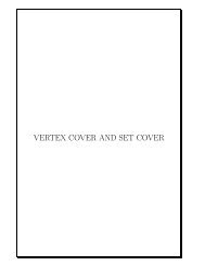
2 A. Delong, L. Gorelick, F. R. Schmidt, O. Veksler and Y. Boykovuser scribbles1 2propose models fromcurrent super-labelingsolve 2-level MRF converged to finalvia α-expansionsub-labelingE=503005 E=4522883 re-estimate all sub-modelsFig. 2. We iteratively propose new models by randomly sampling pixels from superlabels,optimize the resulting two-level MRF, and re-estimate model parameters.We propose a novel energy that unifies these two approaches by incorporatingunsupervised learning into interactive segmentation. We show that thismore descriptive object model leads to better high-level segmentations. In ourformulation, each object (super-label) is automatically decomposed into spatiallycoherent regions where each region is described by a distinct appearance model(sub-label). This results in a two-level MRF with super-labels at the top level thatare partitioned into sub-labels at the bottom. Figure 1 illustrates the main idea.We introduce the hierarchical Potts (hPotts) prior to govern spatial coherenceat both levels of our MRF. The hierarchical Potts prior regularizes boundariesbetween objects (super-label transitions) differently from boundaries within eachobject (sub-label transitions). The unsupervised aspect of our MRF allows appearancemodels of arbitrary complexity and would severely over-fit the imagedata if left unregularized. We address this by incorporating global sparsity priorinto our MRF via the energetic concept of “label costs” [7].Since our framework is based on multi-label MRFs, a natural choice of optimizationmachinery is α-expansion [11, 7]. Furthermore, the number, class, andparameters of each object’s appearance models are not known a priori — in orderto use powerful combinatorial techniques we must propose a finite set of possibilitiesfor α-expansion to select from. We therefore resort to an iterative graph-cutprocess that involves random sampling to propose new models, α-expansion toupdate the segmentation, and re-estimation to improve the current appearancemodels. Figure 2 illustrates our algorithm.The remainder of the paper is structured as follows. Section 2 discusses othermethods for modeling complex appearance, MDL-based segmentation, and relatediterative graph-cut algorithms. Section 3 describes our energy-based formulationand algorithm in formal detail. Section 4 shows applications in interactivebinary/multi-class segmentation and interactive co-segmentation; furthermore itdescribes how our framework easily allows appearance models to come from amixture of classes (GMM, plane, etc.). Section 5 draws an interesting parallelbetween our formulation and multi-class semi-supervised learning in general.2 Related WorkComplex appearance models. The DDMCMC method [6] was the first toemphasize the importance of representing object appearance with complex mod-

Interactive Segmentation with Super-Labels 3els (e.g. splines and texture based models in addition to GMMs) in the contextof unsupervised segmentation. However, being unsupervised, DDMCMC doesnot delineate objects but rather provides low-level segments along with their appearancemodels. Ours is the first multi-label graph-cut based framework thatcan learn a mixture of such models for segmentation.There is an interactive method [10] that decomposes objects into spatiallycoherent sub-regions with distinct appearance models. However, the number ofsub-regions, their geometric interactions, and their corresponding appearancemodels must be carefully designed for each object of interest. In contrast, weautomatically learn the number of sub-regions and their model parameters.MDL-based segmentation. A number of works have shown that minimumdescription length (MDL) is a useful regularizer for unsupervised segmentation,e.g. [5–7]. Our work stands out here in two main respects: our formulationis designed for semi-supervised settings and explicitly weighs the benefit of eachappearance model against the ‘cost’ of its inherent complexity (e.g. number ofparameters). To the best of our knowledge, only the unsupervised DDMCMC [6]method allows arbitrary complexity while explicitly penalizing it in a meaningfulway. However, they use a completely different optimization framework and,being unsupervised, they do not delineate object boundaries.Iterative graph-cuts. Several energy-based methods have employed EM-stylealternation between a graph-cut/α-expansion phase and a model re-estimationphase, e.g. [12, 2, 13, 14, 7]. Like our work, Grab-Cut [2] is about interactive segmentation,though their focus is binary segmentation with a bounding-box interactionrather than scribbles. The bounding box is intuitive and effective formany kinds of objects but often requires subsequent scribble-based interactionfor more precise control. Throughout this paper, we compare our method toan iterative multi-label variant of Boykov-Jolly [1] that we call iBJ. Given userscribbles, this baseline method maintains one GMM per object label and iteratesbetween α-expansion and re-estimating each model.On an algorithmic level, the approach most closely related to ours is the unsupervisedmethod [14, 7] because it also involves random sampling, α-expansion,and label costs. Our framework is designed to learn complex appearance modelsfrom partially-labeled data and differs from [14, 7] in the following respects:(1) we make use of hard constraints and the current super-labeling to guide randomsampling, (2) our hierarchical Potts potentials regularize sub- and superlabelsdifferently, and (3), again, our label costs penalize models based on theirindividual complexity rather than using uniform label costs.3 Modeling Complex Appearance via Super-LabelsWe begin by describing a novel multi-label energy that corresponds to our twolevelMRF. Unlike typical MRF-based segmentation methods, our actual setof discrete labels (appearance models) is not precisely known beforehand andwe need to estimate both the number of unique models and their parameters.Section 3.1 explains this energy formulation in detail, and Section 3.2 describesour iterative algorithm for minimizing this energy.

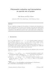
Interactive Segmentation with Super-Labels 5c 2 encourages smoothness among super-labels. This potential is a special case ofour more general class of hierarchical Potts potentials introduced in Appendix 7,but two-level Potts is sufficient for our interactive segmentation applications.For image segmentation we assume c 1 ≤ c 2 , though in general any V withc 1 ≤ 2c 2 is still a metric [11] and can be optimized by α-expansion. Appendix 7gives general conditions for hPotts to be metric. It is commonly known thatsmoothness costs directly affect the expected length of the boundary and shouldbe scaled proportionally to the size of the image. Intuitively c 2 should be largeras it operates on the entire image as opposed to smaller regions that correspondto objects. The weight w pq ≥ 0 of each pairwise term in (1) is computed fromlocal image gradients in the standard way (e.g. [1, 2]).Finally, we incorporate a model-dependent “label costs” [7] to regularize thenumber of unique models in L and their individual complexity. A label cost h lis a global potential that penalizes the use of l in labeling f through indicatorfunction δ l (f) = 1 ⇔ ∃f p = l. There are many possible ways to define the weighth l of a label cost, such as Akaike information criterion (AIC) [16] or Bayesianinformation critierion (BIC) [17]. We use a heuristic described in Section 4.2.3.2 Our SUPERLABELSEG AlgorithmWe propose a novel segmentation algorithm based on the iterative Pearl framework[7]. Each iteration of Pearl has three main steps: propose candidatemodels by random sampling, segment via α-expansion with label costs, andre-estimate the model parameters for the current segmentation. Our algorithmdiffers from [7] as follows: (1) we make use of hard constraints g and the currentsuper-labeling π ◦ f to guide random sampling, (2) our two-level Potts potentialsregularize sub- and super-labels differently, and (3) our label costs penalizemodels based on their individual complexity rather than uniform penalty.The proposal step repeatedly generates a new candidate model l with parametersθ l fitted to a random subsample of pixels. Each model is proposed in thecontext of a particular super-label i ∈ S, and so the random sample is selectedfrom the set of pixels P i = { p | π(f p ) = i } currently associated with i. Eachcandidate l is then added to the current label set L with super-label assignmentset to π(l) = i. A heuristic is used to determine a sufficient number of proposalsto cover the set of pixels P i at each iteration.Once we have candidate sub-labels for every object a naïve approach wouldbe to directly optimize our two-level MRF. However, being random, not all of anobject’s proposals are equally good for representing its appearance. For example,a proposal from a small sample of pixels is likely to over-fit or mix statistics(Figure 3, proposal 2). Such models are not characteristic of the object’s overallappearance but are problematic because they may incidentally match some portionof another object and lead to an erroneous super-label segmentation. Beforeallowing sub-labels to compete over the entire image, we should do our best toensure that all appearance models within each object are relevant and accurate.Given the complete set of proposals, we first re-learn the appearance of eachobject i ∈ S. This is achieved by restricting our energy to pixels that are currentlylabeled with π(f p ) = i and optimizing via α-expansion with label costs [7];

6 A. Delong, L. Gorelick, F. R. Schmidt, O. Veksler and Y. BoykovGMM for 1GMM for 2GMM for 3123graywhitegraywhitegraynot an accurate appearance model for red scribble!whiteFig. 3. The object marked with red has two spatially-coherent appearances: pure gray,and pure white. We can generate proposals for the red object from random patches1–3. However, if we allow proposal 2 to remain associated with the red object, it mayincorrectly claim pixels from the blue object which actually does look like proposal 2.this ensures that each object is represented by an accurate set of appearancemodels. Once each object’s appearance has been re-learned, we allow the objectsto simultaneously compete for all image pixels while continuing to re-estimatetheir parameters. Segmentation is performed on a two-level MRF defined by thecurrent (L, θ, π). Again, we use α-expansion with label costs to select a goodsubset of appearance models and to partition the image. The pseudo-code belowdescribes our SuperLabelSeg algorithm.SuperLabelSeg(g) where g : P → S ∪ {none} is a partial labeling1 L = {} // empty label set with global f, π, θ undefined2 Propose(g) // initialize L, π, θ from user scribbles3 repeat4 Segment(P, L) // segment entire image using all available labels L5 Propose(π ◦f) // update L, π, θ from current super-labeling6 until convergedPropose(z) where z : P → S ∪ {none}1 for each i ∈ S2 P i = { p | z p = i } // set of pixels currently labeled with super-label i3 repeat sufficiently4 generate model l with parameters θ l fitted to random sample from P i5 π(l) = i6 L = L ∪ {l}7 end8 L i = { l | π(l) = i }9 Segment(P i , L i ) // optimize models and segmentation within super-label iSegment( ˆP, ˆL) where ˆP ⊆ P and ˆL ⊆ L1 let f| ˆPdenote current global labeling f restricted to ˆP2 repeat3 f| ˆP= argmin ˆfE( ˆL, θ, π, ˆf) // segment by α-expansion with label costs [7]4 // where we optimize only on ˆf : ˆP → ˆL5 L= L \ { l ∈ ˆL | δ l ( ˆf) = 0} // discard unused models6 θ = argmin θ E( ˆL, θ, π, ˆf) // re-estimate each sub-model params7 until converged

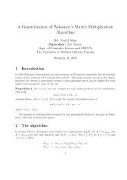
Interactive Segmentation with Super-Labels 7user scribbles sub-labeling our appearance models our segmentation iBJ segmentationFig. 4. Binary segmentation examples. The second column shows our final sub-labelsegmentation f where blues indicate foreground sub-labels and reds indicate backgroundsub-labels. The third column is generated by sampling each I p from model θ fp .The last two columns compare our super-label segmentation π ◦f and iBJ.4 Applications and ExperimentsOur experiments demonstrate the conceptual and qualitative improvement thata two-level MRF can provide. We are only concerned with scribble-based MRFsegmentation, an important class of interactive methods. We use an iterativevariant of Boykov-Jolly [1] (iBJ) as a representative baseline because it is simple,popular, and exhibits a problem characteristic to a wide class of standardmethods. By using one appearance model per object, such methods implicitlyassume that pixels within each object are i.i.d. with respect to its model. However,this is rarely the case, as objects often have multiple distinct appearancesand exhibit strong spatial correlation among their pixels. The main message ofall the experiments is to show that by using multiple distinctive appearancemodels per object we are able to reduce uncertainty near the boundaries of objectsand thereby improve segmentation in difficult cases. We show applicationsin interactive binary/multi-class segmentation and interactive co-segmentation.Implementation details: In all our experiments we used publicly availableα-expansion code [11, 7, 4, 18]. Our non-optimized matlab implementation takeson the order of one to three minutes depending on the size of the image, withthe majority of time spent on re-estimating the sub-model parameters. We usedthe same within- and between- smoothness costs (c 1 = 5, c 2 = 10) in all binary,multi-class and co-segmentation experiments. Our proposal step uses distancebasedsampling within each super-label whereby patches of diameter 3 to 5are randomly selected. For re-estimating model parameters we use the Matlabimplementation of EM algorithm for GMMs and we use PCA for planes. Weregularize GMM covariance matrices to avoid overfitting in (L, a, b) color spaceby adding constant value of 2.0 to the diagonal.4.1 Binary SegmentationFor binary segmentation we assume that the user wishes to segment an objectfrom the background where the set of super-labels (scribble indexes) is definedby S = {F, B}. In this specific case we found that most of the user interaction isspent on removing disconnected false-positive object regions by scribbling overthem with background super-label. We therefore employ a simple heuristic: after

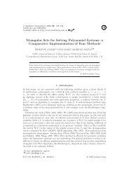
8 A. Delong, L. Gorelick, F. R. Schmidt, O. Veksler and Y. Boykovuser scribbles ours iBJFig. 5. More binary segmentation results showing scribbles, sub-labelings, synthesizedimages, and final cut-outs.iBJoursGMMsoursplaneFig. 6. An image exhibiting gradual changes in color. Columns 2–4 show colors sampledfrom the learned appearance models for iBJ, our two-level MRF restricted to GMMsonly, and ours with both GMMs and planes. Our framework can detect a mix of GMMs(grass,clouds) and planes (sky) for the background super-label (top-right).convergence we find foreground connected components that are not supported bya scribble and modify their data-terms to prohibit those pixels from taking thesuper-label F . We then perform one extra segmentation step to account for thenew constraints. We apply this heuristic in all our binary segmentation results forboth SuperLabelSeg and iBJ (Figures 4, 5, 6). Other heuristics could be easilyincorporated in our energy to encourage connectivity, e.g. star-convexity [19, 20].In Figure 4, top-right, notice that iBJ does not incorporate the floor as partof the background. This is because there is only a small proportion of floor pixelsin the red scribbles, but a large proportion of a similar color (roof) in the bluescribbles. By relying directly on the color proportions in the scribbles, the learnedGMMs do not represent the actual appearance of the objects in the full image.Therefore the ground is considered a priori more likely to be explained by the(wrong) roof color than the precise floor color, giving an erroneous segmentationdespite the hard constraints. Our methods relies on spatial coherence of thedistinct appearances within each object and therefore has a sub-label that fitsthe floor color tightly. This same phenomenon is even more evident in the bottomrow of Figure 5. In the iBJ case, the appearance model for the foreground mixesthe statistics from all scribbled pixels and is biased towards the most dominantcolor. Our decomposition allows each appearance with spatial support (texturedfabric, face, hair) to have good representation in the composite foreground model.

Interactive Segmentation with Super-Labels 9iBJours, GMM onlyours, GMM + planesGMMGMMGMMGMM GMMplaneplaneGMM2 planesdetectedGMMdetectedFig. 7. Our algorithm detects complex mixtures of models, .for example GMMs and planes. The appearance of the above y.xobject cannot be captured by GMMs alone.black white4.2 Complex Appearance ModelsIn natural images objects often exhibit gradual change in hue, tone or shades.Modeling an object with a single GMM in color space [1, 2] makes the implicitassumption that appearance is piece-wise constant. In contrast, our frameworkallows us to decompose an object into regions with distinct appearance models,each from an arbitrary class (e.g. GMM, plane, quadratic, spline). Our algorithmwill choose automatically the most suitable class for each sub-label within anobject. Figure 6 (right) shows such an example where the background is decomposedinto several grass regions, each modeled by a GMM in (L, a, b) color space,and a sky region that is modeled by a plane 3 in a 5-dimensional (x, y, L, a, b)space. Note the gradual change in the sky color and how the clouds are segmentedas a separate ‘white’ GMM.Figure 7 show a synthetic image, in which the foreground object breaks intotwo sub-regions, each exhibiting a different type of gradual change in color. Thiskind of object appearance cannot be captured by a mixture of GMM models.In general our framework can incorporate a wide range of appearance modelsas long as there exists a black-box algorithm for estimating the parameters θ l ,which can be used at the line 6 of Segment. The importance of more complexappearance models was proposed by DDMCMC [6] for unsupervised segmentationin a completely different algorithmic framework. Ours is the first multi-labelgraph-cut based framework that can incorporate such models.Because our appearance models may be arbitrarily complex, we must incorporateindividual model complexity in our energy. Each label cost h l is computedbased on the number of parameters θ l and the number ν of pixels that are tobe labeled, namely h l = 1 2√ ν|θl |. We set ν = #{ p | g p ≠ none } for line 2 of theSuperLabelSeg algorithm and ν = |P| for lines 4,5. Penalizing complexity isa crucial part of our framework because it helps our MRF-based models to avoidover-fitting. Label costs balance the number of parameters required to describethe models against the number of data points to which the models are fit. Whenre-estimating the parameters of a GMM we allow the number of components toincrease or decrease if favored by the overall energy.4.3 Multi-Class SegmentationInteractive multi-class segmentation is a straight-forward application of our energy(1) where the set of super-labels S contains an index for each scribble color.3 In color images a ‘plane’ is a 2-D linear subspace (a 2-flat) of a 5-D image space.

10 A. Delong, L. Gorelick, F. R. Schmidt, O. Veksler and Y. Boykovuser scribbles our sub-labeling our models iBJ labeling iBJ modelsFig. 8. Multi-class segmentation examples. Again, we show the color-coded sublabelingsand the learned appearance models. Our super-labels are decomposed intospatially coherent regions with distinct appearance.Figure 8 shows examples of images with multiple scribbles corresponding to multipleobjects. The resulting sub-labelings show how objects are decomposed intoregions with distinct appearances. For example, in the top row, the basket isdecomposed into a highly-textured colorful region (4-component GMM) and amore homogeneous region adjacent to it (2-component GMM). In the bottomrow, notice that the hair of children marked with blue was so weak in the iBJ appearancemodel that it was absorbed into the background. The synthesized imagessuggest the quality of the learned appearance models. Unlike the binarycase, here we do not apply the post-processing step enforcing connectivity.4.4 Interactive Co-segmentationOur two-level MRFs can be directly used for interactive co-segmentation [3, 21].Specifically, we apply our method to co-segmentation of a collection of similarimages as in [3] because it is a natural scenario for many users. This differs from‘unsupervised’ binary co-segmentation [8, 9] that assumes dissimilar backgroundsand similar-sized foreground objects. Figure 9 shows a collection of four imageswith similar content. Just by scribbling on one of the images our method isable to correctly segment the objects. Note that the unmarked images containbackground colors not present in the scribbled image, yet our method was ableto detect these novel appearances and correctly segment the background intosub-labels.5 Discussion: Super-Labels as Semi-Supervised LearningThere are evident parallels between interactive segmentation and semi-supervisedlearning, particularly among graph cut methods ([1] versus [22]) and randomwalk methods ([23] versus [24]). An insightful paper by Duchenne et al. [25]explicitly discusses this observation. Looking back at our energy and algorithmfrom this perspective, it is clear that we actually do semi-supervised learning appliedto image segmentation. For example, the grayscale image in Figure 7 can bevisualized as points in a 3D feature space where small subsets of points have beenlabeled either blue or red. In addition to making ‘transductive’ inferences, ouralgorithm automatically learned that the blue label is best decomposed into two

Interactive Segmentation with Super-Labels 11image collection our co-segmentation iBJ co-segmentationFig. 9. Interactive co-segmentation examples. Note that our method detected submodelsfor grass, water, and sand in the 1 st and 3 rd bear images; these appearanceswere not present in the scribbled image.linear subspaces (green & purple planes in Figure 7, right) whereas the red labelis best described by a single bi-modal GMM. The number, class, and parametersof these models was not known a priori but was discovered by SuperLabelSeg.Our two-level framework allows each object to be modeled with arbitrarycomplexity but, crucially, we use spatial coherence (smooth costs) and labelcosts to regularize the energy and thereby avoid over-fitting. Setting c 1 < c 2 inour smooth costs V corresponds to a “two-level clustering assumption,” i.e. thatclass clusters are better separated than the sub-clusters within each class. Tothe best of our knowledge, we are first to suggest iterated random samplingand α-expansion with label costs (SuperLabelSeg) as an algorithm for multiclasssemi-supervised learning. These observations are interesting and potentiallyuseful in the context of more general semi-supervised learning.6 ConclusionIn this paper we raised the question of whether GMM/histograms are an appropriatechoice for modeling object appearance. If GMMs and histograms are notsatisfying generative models for a natural image, they are equally unsatisfyingfor modeling appearance of complex objects within the image.To address this question we introduced a novel energy that models complexappearance as a two-level MRF. Our energy incorporates both elementsof interactive segmentation and unsupervised learning. Interactions are used to

12 A. Delong, L. Gorelick, F. R. Schmidt, O. Veksler and Y. Boykovprovide high-level knowledge about objects in the image, whereas the unsupervisedcomponent tries to learn the number, class and parameters of appearancemodels within each object. We introduced the hierarchical Potts prior to regularizesmoothness within and between the objects in our two-level MRF, and weuse label costs to account for the individual complexity of appearance models.Our experiments demonstrate the conceptual and qualitative improvement thata two-level MRF can provide.Finally, our energy and algorithm have interesting interpretations in terms ofsemi-supervised learning. In particular, our energy-based framework can be extendedin a straight-forward manner to handle general semi-supervised learningwith ambiguously-labeled data [26]. We leave this as future work.7 Appendix — Hierarchical PottsIn this paper we use two-level Potts potentials where the smoothness is governedby two coefficients, c 1 and c 2 . This concept can be generalized to a hierarchicalPotts (hPotts) potential that is useful whenever there is a natural hierarchicalgrouping of labels. For example, the recent work on hierarchical context [27]learns a tree-structured grouping of the class labels for object detection; withhPotts potentials it is also possible to learn pairwise interactions for segmentationwith hierarchical context. We leave this as future work.We now characterize our class of hPotts potentials and prove necessary andsufficient conditions for them to be optimized by the α-expansion algorithm [11].Let N = L∪S denote combined set of sub-labels and super-labels. A hierarchicalPotts prior V is defined with respect to an irreducible 4 tree over node set N . Theparent-child relationship in the tree is determined by π : N → S where π(l) givesthe parent 5 of l. The leaves of the tree are the sub-labels L and the interior nodesare the super-labels S. Each node i ∈ S has an associated Potts coefficient c i forpenalizing sub-label transitions that cross from one sub-tree of i to another. AnhPotts potential is a special case of general pairwise potentials over L and can bewritten as an |L|×|L| “smooth cost matrix” with entries V (l, l ′ ). The coefficientsof this matrix are block-structured in a way that corresponds to some irreducibletree. The example below shows an hPotts potential V and its corresponding tree.V(l, l ′ )0 c 1c 5c 1000 c 2 c4c2 0c 5c 40 c 3c 3 0⇔1sub-labels L5super-labels S42 3α β γLet π n (l) denote n applications of the parent function as in π(· · · π(l)). Letlca(l, l ′ ) denote the lowest common ancestor of l and l ′ , i.e. lca(l, l ′ ) = i where4 A tree is irreducible if all its internal nodes have at least two children.5 The root of the tree r ∈ S is assigned π(r) = r.

Interactive Segmentation with Super-Labels 13i = π n (l) = π m (l ′ ) for minimal n, m. We can now define an hPotts potential asV (l, l ′ ) = c lca(l,l ′ ) (4)where we assume V (l, l) = c l = 0 for each leaf l ∈ L. For example, in the treeillustrated above lca(α, β) is super-label 4 and so the smooth cost V (α, β) = c 4 .Theorem 1. Let V be an hPotts potential with corresponding irreducible tree π.V is metric on L ⇐⇒ c i ≤ 2c j for all j = π n (i). (5)Proof. The metric constraint V (β, γ) ≤ V (α, γ) + V (β, α) is equivalent toc lca(β,γ) ≤ c lca(α,γ) + c lca(β,α) (6)for all α, β, γ ∈ L. Because π defines a tree structure, for every α, β, γ thereexists i, j ∈ S such that, without loss of generality,j = lca(α, γ) = lca(β, α), andi = lca(β, γ) such that j = π k (i) for some k ≥ 0.(7)In other words there can be up to two unique lowest common ancestors among(α, β, γ) and we assume ancestor i is in the sub-tree rooted at ancestor j, possiblyequal to j. For any particular (α, β, γ) and corresponding (i, j) inequality (6) isequivalent to c i ≤ 2c j . Since π defines an irreducible tree, for each (i, j) theremust exist corresponding sub-labels (α, β, γ) for which (6) holds. It follows thatc i ≤ 2c j holds for all pairs j = π k (i) and completes the proof of (5). References1. Boykov, Y., Jolly, M.P.: Interactive Graph Cuts for Optimal Boundary and RegionSegmentation of Objects in N-D Images. Int’l Conf. on Computer Vision (ICCV)1 (2001) 105–1122. Rother, C., Kolmogorov, V., Blake, A.: GrabCut: Interactive Foreground Extractionusing Iterated Graph Cuts. In: ACM SIGGRAPH. (2004)3. Batra, D., Kowdle, A., Parikh, D., Luo, J., Chen, T.: iCoseg: Interactive Cosegmentationwith Intelligent Scribble Guidance. In: IEEE Conf. on ComputerVision and Pattern Recognition (CVPR). (2010)4. Kolmogorov, V., Zabih, R.: What Energy Functions Can Be Optimized via GraphCuts. IEEE Trans. on Patt. Analysis and Machine Intelligence 26 (2004) 147–1595. Zhu, S.C., Yuille, A.L.: Region competition: unifying snakes, region growing, andBayes/MDL for multiband image segmentation. IEEE Trans. on Pattern Analysisand Machine Intelligence 18 (1996) 884–9006. Tu, Z., Zhu, S.C.: Image Segmentation by Data-Driven Markov Chain Monte Carlo.IEEE Trans. on Pattern Analysis and Machine Intelligence 24 (2002) 657–6737. Delong, A., Osokin, A., Isack, H., Boykov, Y.: Fast Approximate Energy Minimizationwith Label Costs. Int’l Journal of Computer Vision (2011) (in press).

14 A. Delong, L. Gorelick, F. R. Schmidt, O. Veksler and Y. Boykov8. Rother, C., Minka, T., Blake, A., Kolmogorov, V.: Cosegmentation of Image Pairsby Histogram Matching - Incorporating a Global Constraint into MRFs. In: IEEEConf. on Computer Vision and Pattern Recognition (CVPR). (2006)9. Vicente, S., Kolmogorov, V., Rother, C.: Cosegmentation Revisited: Models andOptimization. In: European Conf. on Computer Vision (ECCV). (2010)10. Delong, A., Boykov, Y.: Globally Optimal Segmentation of Multi-Region Objects.In: Int’l Conf. on Computer Vision (ICCV). (2009)11. Boykov, Y., Veksler, O., Zabih, R.: Fast Approximate Energy Minimization viaGraph Cuts. IEEE Trans. on Pattern Analysis and Machine Intelligence (2001)12. Birchfield, S., Tomasi, C.: Multiway cut for stereo and motion with slanted surfaces.In: Int’l Conf. on Computer Vision. (1999)13. Zabih, R., Kolmogorov, V.: Spatially Coherent Clustering with Graph Cuts. In:IEEE Conf. on Computer Vision and Pattern Recognition (CVPR). (2004)14. Isack, H.N., Boykov, Y.: Energy-based Geometric Multi-Model Fitting. Int’l Journalof Computer Vision (2011) (accepted).15. Lafferty, J., McCallum, A., Pereira, F.: Conditional random fields: Probabilisticmodels for segmenting and labeling sequence data. In: Int’l Conf. on MachineLearning (ICML). (2001)16. Akaike, H.: A new look at statistical model identification. IEEE Trans. on AutomaticControl 19 (1974) 716–72317. Schwarz, G.: Estimating the Dimension of a Model. Annals of Statistics 6 (1978)461–64618. Boykov, Y., Kolmogorov, V.: An Experimental Comparison of Min-Cut/Max-FlowAlgorithms for Energy Minimization in Vision. IEEE Trans. on Pattern Analysisand Machine Intelligence 29 (2004) 1124–113719. Veksler, O.: Star Shape Prior for Graph-Cut Image Segmentation. In: EuropeanConf. on Computer Vision (ECCV). (2008)20. Gulshan, V., Rother, C., Criminisi, A., Blake, A., Zisserman, A.: Geodesic StarConvexity for Interactive Image Segmentation. In: IEEE Conf. on Computer Visionand Pattern Recognition (CVPR). (2010)21. Schnitman, Y., Caspi, Y., Cohen-Or, D., Lischinski, D.: Inducing Semantic Segmentationfrom an Example. In: Asian Conf. on Computer Vision (ACCV). (2006)22. Blum, A., Chawla, S.: Learning from labeled and unlabeled data using graphmincuts. In: Int’l Conf. on Machine Learning. (2001)23. Grady, L.: Random Walks for Image Segmentation. IEEE Trans. on PatternAnalysis and Machine Intelligence 28 (2006) 1768–178324. Szummer, M., Jaakkola, T.: Partially labeled classication with markov randomwalks. In: Advances in Neural Information Processing Systems (NIPS). (2001)25. Duchenne, O., Audibert, J.Y., Keriven, R., Ponce, J., Segonne, F.: Segmentationby transduction. In: IEEE Conf. on Computer Vision and Pattern Recognition(CVPR). (2008)26. Cour, T., Sapp, B., Jordan, C., Taskar, B.: Learning from Ambiguously LabeledImages. In: IEEE Conf. on Computer Vision and Pattern Recognition (CVPR).(2009)27. Choi, M.J., Lim, J., Torralba, A., Willsky, A.S.: Exploiting Hierarchical Contexton a Large Database of Object Categories. In: IEEE Conf. on Computer Visionand Pattern Recognition (CVPR). (2010)