AST242 LECTURE NOTES PART 5 Contents 1. Waves and ...

AST242 LECTURE NOTES PART 5Contents1. Waves and instabilities 11.1. Sound waves – compressive waves in 1D 12. Jeans Instability 53. Stratified Fluid Flows – Waves or Instabilities on a Fluid Boundary 63.1. Surface gravity waves 103.2. Rayleigh-Taylor instability 103.3. Kelvin-Helmholtz Instability 114. Thermal Instability 124.1. Acoustic waves damped by thermal conductivity 144.2. Field Stability Criterion 154.3. An aside on positive and negative feedback 165. Convective Instability 175.1. Schwarzschild criterion and the Brunt-Väisälä frequency 186. Waves traveling in a plane parallel atmosphere 197. Acknowledgements 231. Waves and instabilitiesIn this section we will carry out a series of calculations that are similar in that theyinvolve considering small perturbations and how they evolve. We will often derive adispersion relation and use it to determine if waves are likely to be able to travel orif small perturbations can become unstable and grow. Our first example illustratesthe procedure with sounds waves. In this case there is no instability but we do finda dispersion relation relating wavelengths to frequencies for wave solutions.1.1. Sound waves – compressive waves in 1D. Consider an isentropic ideal fluidwith equation of state p = Kρ γ . Recall Euler’s equation.(1)∂u∂t + u · ∇u = −1 ρ ∇pConsider small perturbations in one dimension about an equilibrium configurationwith zero velocity, u(x, t) = u 1 (x, t) and ρ(x, t) = ρ 0 + ρ 1 (x, t) where u 1 and ρ 1 are1

2 AST242 LECTURE NOTES PART 5both small. We assume that the zeroth order velocity u 0 = 0. We have restrictedthe possible waves to 1 dimension. We also assume that pressure can be describedas p(x, t) = p 0 + p 1 (x, t) where p 0 is independent of time and position. We insertthese expressions in to Euler’s equation∂(2)∂t (u 0 + u 1 ) + (u 0 + u 1 ) ∂∂x (u 0 + u 1 ) = − 1 ∂ρ 0 + ρ 1 ∂x (p 0 + p 1 )1We can approximateρ 0 +ρ 1∼ 1 ρ 0(1 − ρ 1 /ρ 0 )Any term that is a produce of two first order terms is second order so we can dropit. We can also drop zero-th order terms as they should satisfy Euler’s equation ontheir own. Euler’s equation becomes∂u 1(3)∂t + u ∂u 10∂x + u ∂u 01∂x = − 1 ∂p 1ρ 0 ∂x + ρ 1 ∂p 0ρ 2 0 ∂xAs u 0 = 0 we can drop the second term on the left hand side. As u 0 doesn’t dependon position we can drop the third term on the left hand side. As p 0 does not dependon position we can drop the second term on the right hand side. Euler equation nowbecomes∂u 1(4)∂t = − 1 ∂p 1ρ 0 ∂xWe note that(5) dp 1 = ∂p ( )0∂ρ dρ → ∂p 1 ∂p∂x = ∂ρ0∂ρ 1∂x .and Euler’s equation can be written in terms of density and velocity only∂u 1(6)∂t = − 1 ( ) ∂p ∂ρ 1ρ 0 ∂ρ ∂xTo first order in our perturbations Euler’s equation has become(7) u 1,t = − 1 ( ) ∂pρ 0 ∂ρ0ρ 1,x0where ,x refers to a derivative with respect to x. The u · ∇u term is second order inour perturbation strength and so has been dropped. Let’s take the time derivativeof this equation(8) u 1,tt = − 1 ρ 0( ∂p∂ρ)ρ 1,xt0We now use the equation of continuity∂ρ(9)∂t + ∇ · (ρu) = 0

AST242 LECTURE NOTES PART 5 3Following the same procedure of using first order perturbations, conservation of massbecomes(10) ρ 1,t = −ρ 0 u 1,xLet’s take the x derivative of this equation(11) ρ 1,tx = −ρ 0 u 1,xxPutting these together we find(12) u 1,tt =This is a wave equation with solutions(13)(14)( ) ∂pu 1,xx∂ρ0u 1 = A exp(i(kx − ωt))ρ 1 = B exp(i(kx − ωt))for amplitudes A, B. Inserting these wavelike solutions into our equation for conservationof mass and that derived from Euler’s equation we find a dispersion relation( ) ∂p(15) ω 2 =∂ρThe sound speed is√ (∂p )(16) c s =∂ρ0k 20=√γ p ρwhere the derivative is often describe in terms of keeping the entropy fixed. FurthermoreEquation (7) relates the amplitude in velocity to that in density withA = c s B/ρ 0 .The above procedure of using a first order perturbation approximation and lookingfor a dispersion relation is seen again and again in fluid dynamics. It is used forstability analysis, for example in derivation of the Kelvin Helmholtz instability. Thisprocedure is also used to find the dispersion relation for spiral density waves in afluid disk.Consider how we would have done a similar derivation but not restricting thesystem to 1 dimension. Equation 7 (derived from Euler’s equation) becomes(17) u 1,t = − 1 ρ 0( ∂p∂ρand the equation of continuity becomes(18) ρ 1,t = −ρ 0 ∇ · u 1)∇ρ 10

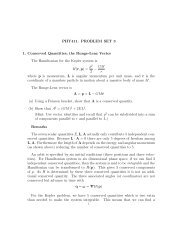
AST242 LECTURE NOTES PART 5 7Figure 1. Two fluids, one lying above the other in a gravitationalfield. The top fluid has horizontal velocity U ′ and the bottom one hasvelocity U. When the top fluid is denser than the bottom fluid ρ ′ > ρthen the boundary is unstable to the Rayleigh-Taylor instability. Whenρ ′ < ρ gravity waves can propagate on the boundary. When U ′ ≠ Uthen the boundary is unstable to the Kelvin-Helmholtz instability.This problem is somewhat more complicated than our previous example of soundwaves as we must consider an interface.Recall Euler’s equation(44)∂u∂t + (u · ∇u)u = −1 ∇p − ∇ΦρWe use the vector identity( ) u2(45) (u · ∇)u = ∇ − u × ∇ × u2If the flow is irrotational we can drop the second term on the right. For an irrotationalflow Euler’s equation becomes( )∂u u2(46)∂t + ∇ = − 1 ∇p − ∇Φ2 ρIf the flow is irrotational then we can use a potential function for the velocity usuch that(47) ∇ψ = −u

AST242 LECTURE NOTES PART 5 9We require that fluid elements not cross the interface, ξ(x, t). This means that(55) u z = − dψ′dz = ∂ξ∂t + U ′ ∂ξ∂xand(56) u z = − dψdz = ∂ξ∂t + U ∂ξ∂xEquation 50 gives partial derivatives∂ξ(57)∂t = −iωAei(kx−ωt)Inserting these into equations 55, 56 we find(58)for z > 0for z < 0.∂ξ∂x = ikAei(kx−ωt)i(kU ′ − ω)A = kφ ′ 1i(kU − ω)A = −kφ 1 .and each is satisfied. So far the above are two equations for three unknowns A, φ ′ 1, φ 1 .However we have another equation derived from Euler’s equation (or Bernoulli’sequation).We can invert equation 49 to solve for pressure((59) p = −ρ − ∂ψ )∂t + u22 + Φ + ρF (t)At the interface we require pressure balance. The gravitational potential at theinterface Φ = gz = gξ so()((60) −ρ ′ − ∂ψ′∂t + u′22 + gξ + ρ ′ F (t) = −ρ − ∂ψ )∂t + u22 + gξ + ρF (t)For large and small z above and below the boundary we assume that perturbationsin the fluid will decay. Because F (t) does not depend on position we can set it tozero.Zeroth order terms should balance, so we need only consider terms that are firstorder in our perturbation quantities. To first order(61) u ′2 → −2U ′ ∂φ′∂xu 2 → −2U ∂φ∂x .Equation 54 implies that ∂ψ′ = ∂φ′ and likewise for ψ and φ. Inserting these expressionsinto our pressure relation (equation 60) and evaluating it at z = 0∂t ∂t( ) ] [ ( ∂(62) ρ[−′ ∂t + U ′ ∂∂φ ′ + gξ = ρ −∂x∂t + U ∂ ) ]φ + gξ .∂x

10 AST242 LECTURE NOTES PART 5Evaluating at z = 0 is equivalent to assuming that the amplitude of perturbationA is very small (specifically A < k −1 ). Using our exponential forms for φ, φ ′ , ξ thisbecomes(63) ρ ′ (−i(kU ′ − ω)φ ′ 1 + gA) = ρ (−i(kU − ω)φ 1 + gA) .Using equations 58 to eliminate φ ′ 1, φ 1 we find an equation where each term is proportionalto A. Dividing this by A we find a dispersion relation that can be put inthe following form(64) ρ(kU − ω) 2 + ρ ′ (kU ′ − ω) 2 = kg(ρ − ρ ′ ).This is our dispersion relation.3.1. Surface gravity waves. For two fluids at rest (U = U ′ = 0) our dispersionrelation is(65) ω = ± √ √ρ − ρgk′ρ + ρ ′If ρ > ρ ′ then ω is real and we have wave-like solutions. In the limit of ρ ′ ≪ ρ (airover water) ω = √ gk and we have surface gravity waves.3.2. Rayleigh-Taylor instability. Consider fluids at rest with ρ ′ > ρ. In this caseω has to be complex which implies that perturbations can grow exponentially andso are unstable. The solution is(66) ω = ±i √ gk√ρ ′ − ρρ + ρ ′with solutions ∝ e ±iωt . We can construct a growth timescale(67) t grow = i|ω| = (gk)−1/2 ∣ ∣∣∣ ρ ′ − ρρ + ρ ′ ∣ ∣∣∣−1/2so we can write solutions as(68) ∝ e ±t/tgrowAs we have assumed uniform acceleration by gravity, this instability could alsotake place in other settings where there is uniform acceleration such as in the shellof a supernova remnant. Outward acceleration is equivalent to inwardly directedgravity.

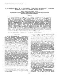
AST242 LECTURE NOTES PART 5 11Figure 2. Kelvin Helmholtz instability grows because of pressure differencescaused by the velocity perturbations. It’s not obvious here,but there must be a small lag between pressure and velocity differencesfor water waves to be excited by wind. If the velocity and pressure perturbationsare exactly in phase then there is no energy transfer betweenmedia.3.3. Kelvin-Helmholtz Instability. We consider the case when fluids are stableto the Rayleigh-Taylor instability but moving with respect to one another. Ourdispersion relation (equation 64) is a quadratic equation for ω. Grouping terms wecan write the dispersion relation as a polynomial of ω,(69) ω 2 (ρ + ρ ′ ) − ω2k(ρU + ρ ′ U ′ ) + k 2 (ρU 2 + ρ ′ U ′2 ) − kg(ρ − ρ ′ ) = 0The quadratic equation gives(70)ω =12(ρ + ρ ′ ) (2k(ρU + ρ′ U ′ )±√4k2 (ρU + ρ ′ U ′ ) 2 − 4(ρ + ρ ′ )(k 2 (ρU 2 + ρ ′ U ′2 ) − kg(ρ − ρ ′ ))).There is no real solution and instability occurs when(71) k > (ρ2 − ρ ′2 )gρρ ′ (U − U ′ ) 2 .Note ω is not necessarily small at the transition point. When gravity is unimportant,we can take g → 0, and then find that all wavelengths are unstable as long as U ′ ≠ U.When ρ > ρ ′ , then gravity stabilizes short k or long wavelengths. The larger k

12 AST242 LECTURE NOTES PART 5are more unstable, consequently the smallest wavelengths grow the fastest, howeversurface tension and other small scale processes can stabilize the smallest wavelengths.4. Thermal InstabilityWe consider the case of the interstellar medium, gas with different temperaturesbut with each phase approximately in pressure equilibrium. There are differentheating and cooling mechanisms. We start with an equation for energy conservation.We would like to work with variables density, temperature and pressure.(72) T dS = de − p dρρ 2For an ideal gas with e = p ρ1γ−1(73) ρT dS = dpγ − 1 −γ pγ − 1 ρ dρUsing the Lagrangian derivative and equating heating rate with that due to thermalconductivity and heating and cooling(74) ρT DSDt = 1 Dpγ − 1 Dt −γ pγ − 1 ρDρDt = ∇ · (λ∇T ) + Q+ (ρ, T ) − Q − (ρ, T )where λ is the thermal conductivity, Q + is the heating rate per unit volume and Q −is the cooling rate. The form of the cooling rate, Q − , is expected to be non-trivial inshape. It contains a peak at about 100K, due to molecular line emission (vibrationaland rotational transitions), and one at 10 5 K due to optical and UV emission linesfrom ions (e.g., bound-free, bound-bound, and during recombination).We include three more equations, the continuity equation (conservation of mass)and Euler’s equation (conservation of momentum) and an equation of state(75) ∂ρ∂t + ∇ · (ρu) = 0(76) ∂u∂t + (u · ∇)u = −1 ρ ∇pp = ρk BT(77)¯m

AST242 LECTURE NOTES PART 5 13We consider perturbations of velocity, density, temperature and pressure in theform(78)ρ(x, t) = ρ 0 + ρ 1 e i(k·x−ωt)p(x, t) = p 0 + p 1 e i(k·x−ωt)T (x, t) = T 0 + T 1 e i(k·x−ωt)u(x, t) = u 1 e i(k·x−ωt)We assume the gas without perturbations is uniform and at rest (u 0 = 0, and p 0 , ρ 0 , T 0independent of x and time).Let consider perturbations to the heating and cooling functions(79) Q(ρ, T ) = Q + (ρ 0 , T 0 ) − Q − (ρ 0 , T 0 ) + Q ρ ρ 1 + Q T T 1so that(80)Q ρ = ∂(Q+ − Q − )∂ρQ T = ∂(Q+ − Q − )∂T∣∣ρ0 ,T 0∣∣ρ0 ,T 0To first order in our perturbations, the continuity equation, Euler’s equation, theequation of state and our equation for conservation of energy become(81)(82)(83)(84)Note γp 0ρ 0−iωρ 1 + ik · u 1 ρ 0 = 0−iωu 1 = −ik p 1p 1= ρ 1+ T 1p 0 ρ 0 T 0− iω (p 1 − γp )0ρ 1 = −λk 2 T 1 + Q T T 1 + Q ρ ρ 1γ − 1 ρ 0= c 2 s where c s is the sound speed. We can dot k with equation (82) to findρ 0(85) ωk · u 1 = k 2 p 1ρ 0and this can be used to eliminate the velocity from the continuity equation(86) ω 2 ρ 1 = k 2 p 1

14 AST242 LECTURE NOTES PART 5Inserting this into the last two perturbation equations( ) ω2ρ 0 ρ1− 1 = T 1(87)k 2 p 0 ρ 0 T 0− iω ( ) ω2(88)γ − 1 k − 2 c2 s ρ 1 = Q T T 1 − λk 2 T 1 + Q ρ ρ 1These can be manipulated to give a dispersion relation(89) − iω ( ) ω2γ − 1 k − 2 c2 s − ( Q T − λk 2) ( )T 0 ω2p 0 k − c2 s= Q 2 ργwhere we have used our definition for sound speed. This differs only in the sign of ωfrom the expression given by Pringle & King (equation 8.10) because of the differentsign in our assumed form for the perturbation. The dispersion relation is a cubicequation in ω. The three roots (real or/and complex) can be studied as a functionof k.Note: We have assumed an ideal gas described with an adiabatic index even thoughwe are considering heating and cooling.4.1. Acoustic waves damped by thermal conductivity. If there is no thermalconductivity, λ = 0, and heating and cooling are negligible (Q ρ = Q T = 0) then thedispersion relation (equation 89) simplifies to(90) ω 2 = k 2 c 2 swhich is the relation for acoustic or sound waves.Let’s consider the dispersion relation when heating balances cooling and we are atan equilibrium point Q ρ = Q T = 0. In this case the dispersion relation becomes(91) iω ( ω 2 − k 2 c 2 s)= λk2 T 0ρ 0(γ − 1) ( ω 2 − k 2 c 2 sγ −1)If we assume that λ is small we can try a solution ω = kc s + x where x is small. Tofirst order in λ and x(92)(93)Thusi2k 2 c 2 sx = λk 2 T 0ρ 0(γ − 1) 2 γ −1 k 2 c 2 sx = − iλ 2T 0ρ 0(γ − 1) 2 γ −1(94) ω = c s k − iδ δ = λ 2T 0ρ 0(γ − 1) 2 γ −1

AST242 LECTURE NOTES PART 5 15with δ > 0. With our form for the perturbations ∝ exp(i(k · x − ωt) we find that ourperturbations exponentially damp due to thermal conductivity.Note that δ is not small if k is sufficiently large. Hence our assumption that δis small is only satisfied for moderate values of k. For k sufficiently large (or oversufficiently small distances) perturbations are rapidly damped due to conduction.The parameter δ has units of inverse time. We can estimate how much the amplitudeis reduced per wavelength traveled with the factor e −δP where P is the period,P = 2π = 2π .ω c sk4.2. Field Stability Criterion. We consider slow changes or small ω. In this limitω ≪ kc s and our dispersion relation (equation 89) reduces to(95)We can rewrite this asiωγ − 1 c2 s + ( Q T − λk 2) T 0p 0c 2 sγ = Q ρ(96) iω = γ − 1 ( )Qρ ρ 0 − Q T T 0 + λk 2 T 0 .γp 0 The ISM is nearly in pressure equilibrium. Since p ∝ ρT we can use ∂ρ ∣∂T p= − ρ Tand∂Q(97)∂ ln T ∣ = Q T T + Q ρ T ∂ρp∂T ∣ = Q T T − Q ρ ρpThus our dispersion relation (equation 95) becomes[(98) −iω = γ − 1]∂Qγp 0 ∂ ln T ∣ − λk 2 T 0pIn the case of no conductivity (λ = 0) there is instability when(99) instability ⇐⇒ ∂Q∂ ln T ∣ > 0pThis is called the Field stability criterion.Let us consider the Field stability criterion physically. Pressure equilibrium isexpected otherwise there will be large velocities generated and mixing. If increasingthe temperature increases the heating rate then the temperature will continue torise and we will have instability. If increasing the temperature decreases the heatingrate then we will have convergence to a stable situation. For the second case, givingstability, we have negative feedback. For the first case, giving instability, we havepositive feedback. I note that there can be instability even in the negative feedbackcase if the feedback (heating or cooling) is delayed, a situation that we have not

16 AST242 LECTURE NOTES PART 5taken into account here but does happen for example when star formation heats orperturbs the medium affecting future generations of stars.When there is conductivity and k is large there is stability even when the stabilitycriterion shown in equation (99) is violated. In this case the thermal conductivitysmoothes or damps temperature fluctuations faster than they can grow. We candefine a critical wavevector by setting ω = 0 in equation (99) and solving for k(100) k 2 F ≡ 1λT 0∂Q∂ ln TThe Field length λ F ≡ 2π/k F . For wavelengths larger than the critical one perturbationswill grow. Small perturbations are smoothed out by the conductivity and sostabilized.4.3. An aside on positive and negative feedback. The very simplest systemdΣ(101)dt = f(Σ)can achieve equilibrium near a fixed point Σ ∗ where f(Σ ∗ ) = 0. Expanding aboutthe fixed point and letting x = Σ − Σ ∗dx(102)dt = f ′ (Σ ∗ )xThis has an exponential solution that is exponentially decaying to the fixed point iff ′ (Σ ∗ ) < 0. If the derivative is negative we say the system has negative feedbackand we expect a stable system. Otherwise we say the system has positive feedbackand we expect it to be unstable. Note that f ′ (Σ) is in units of inverse time and sodefines a decay or growth timescale;(103) t decay = − 1f ′ (Σ) .A system with delayed feedback might look like thisdΣ(t)(104)= f(Σ(t − τ))dtso that its rate of change depends on the density Σ at a time τ in the past. Wecould imagine a complicated function f that depends on Σ at various times. Thereis a class of differential equations called delayed differential equations that can beemployed. Instability can occur even when there is negative feedback in systems withdelayed feedback. Instability or oscillating solutions can occur when the feedbackdelay timescale τ exceeds the timescale for decay to equilibrium, t decay . For exampleπ(105) ˙Σ = − Σ(t − τ)2τ∣∣p

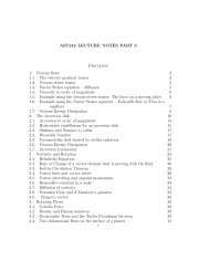
has solution(106) Σ ∝ sinAST242 LECTURE NOTES PART 5 17( ) πt.2τ. Oscillating solutions can have frequencies that period related to the delay; hereP ∼ 4τ.5. Convective InstabilityFigure 3. A small fluid element is displaced by δz. Originally it hadpressure and density p, ρ. At its new location the ambient pressureand density are p ′ , ρ ′ . We let the fluid element expand or contractto reach pressure equilibrium at its new location without exchangingheat. Its new density is ρ ∗ . If ρ ∗ > ρ ′ and the fluid element is denserthan the ambient medium then it will sink back to its original location.Otherwise it will keep rising and the system is convectively unstable.Consider a small fluid element that is located in fluid that is in hydrostatic equilibriumin a gravitational field. Our fluid element starts in equilibrium with pressureand density p, ρ. We then displace it by a vertical amount δz. At this new positionthe ambient pressure and density are slightly different with pressure and densityp ′ , ρ ′ . When we displaced our fluid element it may have contracted or expanded. Ifits new density ρ ∗ is larger than the new ambient value ρ ′ then the fluid elementwill sink back to its original position. In this case the system is stable. If the newfluid element density ρ ∗ is lower than the new ambient value then the fluid elementis buoyant and we say the system is convectively unstable.How are we going to let the fluid element change? We let it remain in pressureequilibrium with its surroundings. This means its new pressure is p ′ . We don’tallow it to heat or cool while we displace it. This is equivalent to assuming that

18 AST242 LECTURE NOTES PART 5heat exchange is slow. This is equivalent to moving the fluid element adiabatically.Because we consider adiabatic changes p ∝ ρ γ and( ) γ ( )p ∗(107)p = p′p = ρ∗p′ 1/γor ρ ∗ = ρρpThe pressure gradient for our atmosphere is dp . If we go up by δz from a particulardzlocation, then the ambient pressure and density are(108) p ′ = p + dpdz δzρ′ = ρ + dρdz δz.We insert p ′ into our previous equation finding( ) p′ 1/γρ ∗ = ρp( p + dp/dzδz= ρp(= ρ 1 + 1 )dpγp dz δz(109)= ρ + ρ dpγp dz δz.) 1/γThe difference in densities( ρ(110) ρ ∗ − ρ ′ dp=γp dz − dρ )δzdzThe system is stable if ρ ∗ > ρ ′ or(111)ρ dpγp dz > dρdzThe stability criterion is often called the Schwarzschild criterion but it is usuallyexpressed in terms of temperature.5.1. Schwarzschild criterion and the Brunt-Väisälä frequency. Using an idealgas p ∝ ρT orExpanding the derivative dρdz ,ρ ∝ p T .(112) ρ ′ = ρ + dρ [ ρdz δz = ρ + dpp dz − ρ T]dTδz.dz

AST242 LECTURE NOTES PART 5 19We can modify equation 110[(113) ρ ∗ − ρ ′ = −(1 − γ −1 ) ρ dpp dz + ρ T]dTδzdzmust be positive for stability. Both dT dpand are expected to be negative in andz dzatmosphere. The first term dominates and the medium is stable if(114)dT∣ dz ∣ < (1 − γ−1 ) T dpρ ∣dz∣ .This is the Schwarzschild criterion.The force per unit volume acting on the displaced fluid element is g(ρ ∗ − ρ) wherethe difference in densities is given by equation (113). An equation of motion(115) ρ d2 (δz)= −g(ρ − ρdt 2 ∗ )ord 2 (δz)(116)= − g [−(1 − γ −1 ) ρ dpdt 2 ρp dz + ρ TThe Brunt-Väisälä frequency, N,(117) N 2 = g [ dTT dz − (1 − γ−1 ) T ]dpp dz]dTδzdzgives the frequencies of small oscillations when the system is stable. These are calledinternal gravity waves to differentiate them from surface waves. The frequency isthat for buoyant oscillations. The Brunt-Väisälä frequency can also be written (seeequation 110)(118) N 2 = g ( ρ dpρ γp dz − dρ )dzFor an isothermal gas γ = 1, the pressure is proportional to the density, p ∝ ρ,and the temperature gradient is zero, dT/dz = 0. In an isothermal atmospherethe Brunt-Väisälä frequency vanishes; N = 0. An atmosphere with a steep temperaturegradient is likely to be convective (with negative N 2 and not satisfying theSchwarzchild criterion for stability) whereas one with a shallow temperature gradientshould be stable (and with positive N 2 ).6. Waves traveling in a plane parallel atmosphereThe background setting is an atmosphere in hydrostatic equilibrium. We encountertwo restoring forces for small perturbations: pressure and buoyancy. We suspect thatwaves can travel at the sound speed, c s if they are primarily acoustic in nature, andwith a frequency that is related to the Brunt-Väisälä frequency, N if they are buoyant

20 AST242 LECTURE NOTES PART 5in nature. We expect a dispersion relation that has limits of ω = c s k for acousticwaves and ω = N for internal gravity waves.Our zero-th order or equilibrium solution has density and pressure ρ 0 (z) and p 0 (z)related via hydrostatic equilibrium(119)dp 0dz = −ρ 0gwhere g is the gravitational acceleration. Mass conservation to first order(120)∂ρ 1∂t + ρ 0∇ · u 1 + ρ 1 ∇ · u 0 + u 0 · ∇ρ 1 + u 1 · ∇ρ 0 = 0We drop terms with u 0 as the equilibrium system is static and u 0 = 0. The gradient∇ρ 0 only contains a z component.(121)∂ρ 1∂t + u ∂ρ 0z1∂z + ρ 0∇ · u 1 = 0Euler’s equation for momentum conservation, again to first order(122)∂u 1∂t= ρ 1 dp 0ρ 2 0 dz ẑ − 1 ∇p 1ρ 0and we have ignored the variation of the gravitational acceleration. We have usedthe fact that the unperturbed pressure gradient is in the z direction.We have a system that in which two directions x, y differ from the other, z, wheregradients in the ambient pressure and density exist. Let our velocity perturbation(123)u 1 = (u, v, w).Let our perturbations be functions of z that are wavelike in the other two dimensions,(124) u, v, w, ρ 1 , p 1 ∝ exp i(ωt − k x x − k y y)with(125) k ⊥ ≡√k 2 x + k 2 y.The equation for conservation of mass (equation 121) becomes(126) iωρ 1 + w dρ [0dz + ρ 0 −i(k x u + k y v) + dw ]= 0dz

Euler’s equation (equation 122) becomesAST242 LECTURE NOTES PART 5 21ωu = 1 ρ 0k x p 1(127)ωv = 1 ρ 0k y p 1iωw = ρ 1 dp 0ρ 2 0 dz − 1 dp 1ρ 0 dzWe can use the first two expressions above to remove u, v from equation (126).(128) iωρ 1 + w dρ 0dz − i(k2 x + ky) 2 p 1ω + ρ dw0dz = 0We now relate pressure perturbations to density perturbations. We assume thatperturbations are locally adiabatic. This condition can be written( ) ( )∂ p p(129)+ (u · ∇) = 0∂t ρ γ ρ γExpanding this∂p(130)∂t − ∂ρc2 s∂t + (u · ∇)p − c2 s(u · ∇)ρ = 0where c 2 s = γp/ρ. To first order(131)or(132) iω(p 1 − c 2 sρ 1 ) + w∂p 1∂t − ∂ρ 1c2 s∂t + w dp 0dz − c2 sw dρ 0dz = 0( dp0dz − c2 s)dρ 0= 0.dzRemember that c 2 s depends on z! The right terms can be written in terms of theBrunt-Väisälä frequency (equation 118)(133) iω(p 1 − c 2 sρ 1 ) + w ρ 0c 2 sN 2Use hydrostatic equilibrium(134) g = − 1 ρ 0dp 0dzand the Brunt-Väisälä frequency(135) − dρ 0dz = N 2 ρ 0g+ gρ 0c 2 sg= 0.

22 AST242 LECTURE NOTES PART 5we can remove vertical derivatives of ρ 0 and p 0 . Pulling together our equations(equation 128,127 and 133)(136)( N2iωρ 1 − wρ 0g + g )− ik 2 p 1c 2 ⊥s ω + ρ dw0dz= 0(137)(138)iωw + gρ 1+ 1 dp 1ρ 0 ρ 0 dziω(p 1 − c 2 sρ 1 ) + w ρ 0c 2 sN 2g= 0= 0The above involve vertical derivatives of w and p 1 but not ρ 1 so we can reduce theproblem to two coupled first order equations involving p 1 and w. These can bestudied by themselves with all variables depending on z.One can do a local analysis assuming that wavelengths are smaller than the atmospherescale height. In this case we can assume that ρ 1 , p 1 , w all depend on e ikzz andrequire that k z ≫ g/c 2 s. In this limit we find a local dispersion relation(139) ω 4 − (N 2 + k 2 c 2 s)ω 2 + N 2 k 2 ⊥c 2 s = 0with(140) k 2 = k 2 ⊥ + k 2 zThere are two separated regimes on a plot of ω 2 vs k⊥ 2 for allowed wave propagation(see Figure 4). There is a higher frequency set with ω 2 > N 2 which are known asp-waves and a lower frequency set which are known as g-waves. The acoustic orp-waves have phase velocities (ω/k) greater than the sound speed and the buoyancyor g-waves have phase velocities below the sound speed.In the limit of high ω, we find ω 2 ∼ N 2 + k 2 c 2 s.In the limit of high ω, k, we find ω 2 ∼ k 2 c 2 s and the waves are acoustic.In the limit of low ω, we find ω 2 ∼ N 2 k⊥ 2 c2 s.N 2 +k 2 c 2 sIn the limit of low ω, k, we find ω 2 ∼ k 2 c 2 s and the waves are acoustic.In the limit of low ω and high k we find ω 2 ∼ N 2 k⊥2 .k 2Some notes: Apparently low g waves are incompressible, (but why?) and thephase velocity is perpendicular to the group velocity (make this clear?). Why is thisimportant?If there are boundary conditions then there is a discrete set of modes. I have triedto be careful here not to use the word ‘mode’ instead of the word ‘wave’. Abovewe have a local dispersion relation. Prior to that we had coupled equations thatdepended on depth in the atmosphere. For a whole body one would not necessarilyuse a plane parallel approximation but instead consider the equations as a functionof radius, and if the system is rotating, as a function of latitude. Certain frequencies

AST242 LECTURE NOTES PART 5 23Figure 4. The grey regions show the allowed regions for wave propagationbased on the local dispersion relation for waves in a planeparallel atmosphere. Here N is the Brunt-Väisälä frequency and c sthe sound speed. Waves propagating with ω > N are p-waves andthose propagating with ω < N are g-waves.will resonate and these can be called modes. Observations of the spectrum of modescan be used to probe the structure of the object. For example thousands of modeshave been measured on the Sun. The study of these waves and modes is calledhelioseismology. The internal structures of the Sun, Earth and stars are tightlyconstrained by the properties of the modes of oscillation.7. AcknowledgementsInstability at an interface following Clarke and Carswell. Thermal instabilityfollowing Pringle and King. Convective instability following Clarke and Carswell.Waves in atmospheres following Pringle and King.