Lyapunov exponents - ChaosBook.org

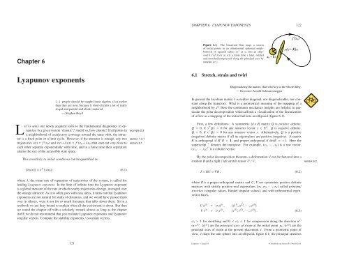
CHAPTER 6. LYAPUNOV EXPONENTS 122Chapter 6Figure 6.1: The linearized flow maps a swarmof initial points in an infinitesimal spherical neighborhoodof squared radius δx 2 at x 0 into an ellipsoidδx⊤ (J ⊤ J)δx at x(t) a finite time t later, rotatedand stretched/compressed along the principal axes bystreches{σ j} .x0000000111111100000001111111000000011111110000000111111100000001111111000000011111110000000111111100000001111111000000011111110000011111 000000011111110000011111 000000011111110000011111 000000011111110000011111 000000011111110000011111 000000011111110000011111 000000011111110000011111 000000011111110000011111 000000011111110000011111 000000011111110000011111111111111111111111111+ δ00000001111111 x0000000111111100000001111111000000011111110000000111111100000001111111000000011111110000000111111100000001111111t0f ( )x(t)+ Jδxx 0Lyapunov exponentsL[...] people should be taught linear algebra a lot earlierthan they are now, because it short-circuits a lot of reallystupid and painful and idiotic material.— Stephen Boydetusapply our newly acquired tools to the fundamental diagnostics in dynamics:Is a given system ‘chaotic’? And if so, how chaotic? If all points in example 2.3a neighborhood of a trajectory converge toward the same orbit, the attractoris a fixed point or a limit cycle. However, if the attractor is strange, any two section 1.3.1trajectories x(t)= f t (x 0 ) and x(t)+δx(t)= f t (x 0 +δx 0 ) that start out very close to remark 6.1each other separate exponentially with time, and in a finite time their separationattains the size of the accessible state space.This sensitivity to initial conditions can be quantified as‖δx(t)‖≈e λt ‖δx 0 ‖ (6.1)whereλ, the mean rate of separation of trajectories of the system, is called theleading Lyapunov exponent. In the limit of infinite time the Lyapunov exponentis a global measure of the rate at which nearby trajectories diverge, averaged overthe strange attractor. As it so often goes with easy ideas, it turns out that Lyapunovexponents are not natural for study of dynamics, and we would have passed themover in silence, were it not for so much literature that talks about them. So in atextbook we are duty bound to explain what all the excitement is about. But thenwe round the chapter off with a scholarly remark almost as long as the chapteritself: we do not recommend that you evaluate Lyapunov exponents and Lyapunovsingular vectors. Compute the stability exponents/ covariant vectors.1216.1 Stretch, strain and twirlDiagonalizing the matrix: that’s the key to the whole thing.— Governor Arnold SchwarzeneggerIn general the Jacobian matrix J is neither diagonal, nor diagonalizable, nor constantalong the trajectory. What is a geometrical meaning of the mapping of aneighborhood by J? Here the continuum mechanics insights are helpful, in particularthe polar decomposition which affords a visualization of the linearizationof a flow as a mapping of the initial ball into an ellipsoid (figure 6.1).First, a few definitions: A symmetric [d× d] matrix Q is positive definite,Q > 0, if x ⊤ Qx > 0 for any nonzero vector x ∈ R d . Q is negative definite,Q < 0, if x ⊤ Qx < 0 for any nonzero vector x. Alternatively, Q is a positive(negative) definite matrix if all its eigenvalues are positive (negative). A matrixR is orthogonal if R ⊤ R = 1, and proper orthogonal if det R = +1. Here thesuperscript ⊤ denotes the transpose. For example, (x 1 ,···, x d ) is a row vector,(x 1 ,···, x d ) ⊤ is a column vector.By the polar decomposition theorem, a deformation J can be factored into arotation R and a right/ left stretch tensor U/ V, remark 6.2J= RU= VR, (6.2)where R is a proper-orthogonal matrix and U, V are symmetric positive definitematrices with strictly positive real eigenvalues{σ 1 ,σ 2 ,···,σ d } called principalstretches (singular values, Hankel singular values), and with orthonormal eigenvectorbases,U u (i) = σ i u (i) , {u (1) , u (2) ,···,u (d) }V v (i) = σ i v (i) , {v (1) , v (2) ,···,v (d) }. (6.3)σ i > 1 for stretching and 0

CHAPTER 6. LYAPUNOV EXPONENTS 123CHAPTER 6. LYAPUNOV EXPONENTS 124are then the lengths of the semiaxes of this ellipsoid. The rotation matrix R carriesthe initial axes of strain into the present ones, V= RUR ⊤ . The eigenvalues of theremark 6.1δx0x(0)δx1x(t 1)right Cauchy-Green strain tensor: J ⊤ J= U 2left Cauchy-Green strain tensor: J J ⊤ = V 2 (6.4)are{σ 2 j }, the squares of principal stretches. example 6.2Figure 6.2: A long-time numerical calculation of theleading Lyapunov exponent requires rescaling the distancein order to keep the nearby trajectory separationwithin the linearized flow range.x(t ) 2δ x26.2 Lyapunov exponentsp. 129(J. Mathiesen and P. Cvitanović)The mean growth rate of the distance‖δx(t)‖/‖δx 0 ‖ between neighboringtrajectories (6.1) is given by the leading Lyapunov exponent which can be estimatedfor long (but not too long) time t asλ≃ 1 t ln‖δx(t)‖ ‖δx(0)‖(6.5)For notational brevity we shall often suppress the dependence of quantities suchasλ=λ(x 0 , t),δx(t)=δx(x 0 , t) on the initial point x 0 . One can use (6.5) as is,take a small initial separationδx 0 , track the distance between two nearby trajectoriesuntil‖δx(t 1 )‖ gets significantly big, then record t 1 λ 1 = ln(‖δx(t 1 )‖/‖δx 0 ‖),rescaleδx(t 1 ) by factorδx 0 /δx(t 1 ), and continue add infinitum, as in figure 6.2,with the leading Lyapunov exponent given by1λ= limt→∞ t∑ ∑t i λ i , t= t i . (6.6)iiDeciding what is a safe ’linear range’, the distance beyond which the separationvectorδx(t) should be rescaled, is a dark art.We can start out with a smallδx and try to estimate the leading Lyapunov exponentλfrom (6.6), but now that we have quantified the notion of linear stabilityin chapter 4, we can do better. The problem with measuring the growth rate of thedistance between two points is that as the points separate, the measurement is lessand less a local measurement. In the study of experimental time series this mightbe the only option, but if we have equations of motion, a better way is to measurethe growth rate of vectors transverse to a given orbit.Given the equations of motion, for infinitesimalδx we know theδx i (t)/δx j (0)ratio exactly, as this is by definition the Jacobian matrixlimδx(0)→0δx i (t)δx j (0) = ∂x i(t)∂x j (0) = Jt i j (x 0),so the leading Lyapunov exponent can be computed from the linearization (4.16)1λ(x 0 )= limt→∞ t ln⇑ Jt (x 0 )δx 0⇑ 1= lim‖δx 0 ‖ t→∞ 2t ln(ˆn ⊤ J t⊤ J t ˆn ) . (6.7)In this formula the scale of the initial separation drops out, only its orientationgiven by the initial orientation unit vector ˆn=δx 0 /‖δx 0 ‖ matters. If one does notcare about the orientation of the separation vector between a trajectory and its perturbation,but only its magnitude, one can interpret⇑ J t δx 0⇑ 2 =δx 0 ⊤ (J t⊤ J t )δx 0 ,as the error correlation matrix. In the continuum mechanics language, the rightCauchy-Green strain tensor J ⊤ J (6.4) is the natural object to describe how linearizedneighborhoods deform. In the theory of dynamical systems the stretchesof continuum mechanics are called the finite-time Lyapunov or characteristic exponents,λ(x 0 , ˆn; t)= 1 t ln⇑ Jt ˆn⇑= 1 2t ln(ˆn ⊤ J t⊤ J t ˆn ) . (6.8)They depend on the initial point x 0 and on the direction of the unit vector ˆn,‖ ˆn‖=1 at the initial time. If this vector is aligned along the ith principal stretch,ˆn=u (i) , then the corresponding finite-time Lyapunov exponent (rate of stretching)is given byλ j (x 0 ; t)=λ(x 0 , u ( j) ; t)= 1 t lnσ j(x 0 ; t). (6.9)We do not need to compute the strain tensor eigenbasis to determine the leadingLyapunov exponent,1λ(x 0 , ˆn)= limt→∞ t ln⇑ 1Jt ˆn⇑= limt→∞ 2t ln(ˆn ⊤ J t⊤ J t ˆn ) , (6.10)Lyapunov - 12aug2013 ChaosBook.org version15.6, Mar 15 2015Lyapunov - 12aug2013 ChaosBook.org version15.6, Mar 15 2015

CHAPTER 6. LYAPUNOV EXPONENTS 125CHAPTER 6. LYAPUNOV EXPONENTS 126Figure 6.3: A numerical computation of the logarithmof the stretch ˆn ⊤ (J t⊤ J t )ˆn in formula (6.10) for theRössler flow (2.27), plotted as a function of the Rösslertime units. The slope is the leading Lyapunov exponentλ≈0.09. The exponent is positive, so numerics lendscredence to the hypothesis that the Rössler attractor ischaotic. The big unexplained jump illustrates perils ofLyapunov exponents numerics. (J. Mathiesen)0.0 0.5 1.0 1.5 2.0 2.50 5 10 15 20telliptic islands and chaotic regions, a chaotic trajectory gets captured in the neighborhoodof an elliptic island every so often and can stay there for arbitrarily longtime; as there the orbit is nearly stable, during such episode ln|σ p,1 (x 0 , t)|/t candip arbitrarily close to 0 + . For state space volume non-preserving flows the trajectorycan traverse locally contracting regions, and ln|σ p,1 (x 0 , t)|/t can occasionallygo negative; even worse, one never knows whether the asymptotic attractor is periodicor ‘chaotic’, so any finite time estimate ofλmight be dead wrong. exercise 6.3as expanding the initial orientation in the strain tensor eigenbasis (6.3), ˆn= ∑ (ˆn·u (i) )u (i) , we haveRésuméˆn ⊤ J t⊤ J t ˆn=d∑ ((ˆn·u (i) ) 2 σ 2 i= (ˆn·u (1) ) 2 σ 2 1 1+O(σ22/σ 2 1 )) ,i=1with stretches ordered by decreasing magnitude,σ 1 >σ 2 ≥σ 3···. For long timesthe largest stretch dominates exponentially in (6.10), provided the orientation ˆn ofthe initial separation was not chosen perpendicular to the dominant expandingeigen-direction u (1) . Furthermore, for long times J t ˆn is dominated by the largeststability multiplierΛ 1 , so the leading Lyapunov exponent isλ(x 0 )1{ = lim lnt→∞⇑ ˆn·e (1) ⇑+ln|Λ 1 (x 0 , t)|+O(e −2(λ1−λ2)t ) }t1= limt→∞ t ln|Λ 1(x 0 , t)|, (6.11)whereΛ 1 (x 0 , t) is the leading eigenvalue of J t (x 0 ). The leading Lyapunov exponentnow follows from the Jacobian matrix by numerical integration of (4.10). Theequations can be integrated accurately for a finite time, hence the infinite time limitof (6.7) can be only estimated from a finite set of evaluations of 1 2 ln(ˆn⊤ J t⊤ J t ˆn) asfunction of time, such as figure 6.3 for the Rössler flow (2.27).As the local expansion and contraction rates vary along the flow, the temporaldependence exhibits small and large humps. The sudden fall to a low valuein figure 6.3 is caused by a close passage to a folding point of the attractor, anillustration of why numerical evaluation of the Lyapunov exponents, and provingthe very existence of a strange attractor is a difficult problem. The approximatelymonotone part of the curve you can use (at your own peril) to estimate the leadingLyapunov exponent by a straight line fit.As we can already see, we are courting difficulties if we try to calculate theLyapunov exponent by using the definition (6.11) directly. First of all, the statespace is dense with atypical trajectories; for example, if x 0 happens to lie on aperiodic orbit p,λwould be simply ln|σ p,1 |/T p , a local property of cycle p, nota global property of the dynamical system. Furthermore, even if x 0 happens tobe a ‘generic’ state space point, it is still not obvious that ln|σ p,1 (x 0 , t)|/t shouldbe converging to anything in particular. In a Hamiltonian system with coexistingLet us summarize the ‘stability’ chapters 4 to 6. A neighborhood of a trajectorydeforms as it is transported by a flow. In the linear approximation, the stabilitymatrix A describes the shearing/compression/ expansion of an infinitesimalneighborhood in an infinitesimal time step. The deformation after a finite time tis described by the Jacobian matrix J t , whose eigenvalues (stability multipliers)depend on the choice of coordinates.Floquet multipliers and eigen-vectors are intrinsic, invariant properties of finitetime,compact invariant solutions, such as periodic orbits and relative periodicorbits; they are explained in chapter 5. Stability exponents [6.1] are the correspondinglong-time limits estimated from typical ergodic trajectories.Finite-time Lyapunov exponents and the associated principal axes are definedin (6.8). Oseledec Lyapunov exponents are the t→∞ limit of these.CommentaryRemark 6.1 Lyapunov exponents are uncool, and ChaosBook does not use them atall. Eigenvectors/ eigenvalues are suited to study of iterated forms of a matrix, suchas Jacobian matrix J t or exponential exp(tA), and are thus a natural tool for study ofdynamics. Principal vectors are not, they are suited to study of the matrix J t itself. Thepolar (singular value) decomposition is convenient for numerical work (any matrix, squareor rectangular, can be brought to such form), as a way of estimating the effective rank ofmatrix J by separating the large, significant singular values from the small, negligiblesingular values.Lorenz [6.2, 6.3, 6.4] pioneered the use of singular vectors in chaotic dynamics. Wefound the Goldhirsch, Sulem and Orszag [6.1] exposition very clear, and we also enjoyedHoover and Hoover [6.5] pedagogical introduction to computation of Lyapunov spectraby the method of Lagrange multipliers. Greene and Kim [6.6] discuss singular valuesvs. Jacobian matrix eigenvalues. While they conclude that “singular values, rather thaneigenvalues, are the appropriate quantities to consider when studying chaotic systems,”we beg to differ: their Fig. 3, which illustrates various semiaxes of the ellipsoid in thecase of Lorenz attractor, as well as the figures in ref. [6.7], are a persuasive argument fornot using singular values. The covariant vectors are tangent to the attractor, while theprincipal axes of strain point away from it. It is the perturbations within the attractor thatLyapunov - 12aug2013 ChaosBook.org version15.6, Mar 15 2015Lyapunov - 12aug2013 ChaosBook.org version15.6, Mar 15 2015

CHAPTER 6. LYAPUNOV EXPONENTS 127CHAPTER 6. LYAPUNOV EXPONENTS 128describe the long-time dynamics; these perturbations lie within the subspace spanned bythe leading covariant vectors.That is the first problem with Lyapunov exponents: stretches{σ j } are not related tothe Jacobian matrix J t eigenvalues{Λ j } in any simple way. The eigenvectors{u ( j) } ofstrain tensor J ⊤ J that determine the orientation of the principal axes, are distinct fromthe Jacobian matrix eigenvectors{e ( j) }. The strain tensor J ⊤ J satisfies no multiplicativesemigroup property such as (4.20); unlike the Jacobian matrix (5.3), the strain tensorJ ⊤r J r for the rth repeat of a prime cycle p is not given by a power of J ⊤ J for the singletraversal of the prime cycle p. Under time evolution the covariant vectors map forwardas e ( j) → J e ( j) (transport of the velocity vector (4.9) is an example). In contrast, theprincipal axes have to be recomputed from the scratch for each time t.If Lyapunov exponents are not dynamical, why are they invoked so frequently? Onereason is fear of mathematics: the monumental and therefore rarely read Oseledec [6.8,6.9] Multiplicative Ergodic Theorem states that the limits (6.7–6.11) exist for almost allpoints x 0 and vectors ˆn, and that there are at most d distinct Lyapunov exponentsλ i (x 0 )as ˆn ranges over the tangent space. To intimidate the reader further we note in passingthat “moreover there is a fibration of the tangent space T x M, L 1 (x)⊂L 2 (x)⊂···⊂L r (x)=T x M, such that if ˆn∈ L i (x)\ L i−1 (x) the limit (6.7) equalsλ i (x).” Oseledec proofis important mathematics, but the method is not helpful in elucidating dynamics.The other reason to study singular vectors is physical and practical: Lorenz [6.2, 6.3,6.4] was interested in the propagation of errors, i.e., how does a cloud of initial pointsx(0)+δx(0), distributed as a Gaussian with covariance matrix Q(0)=〈δx(0)δx(0) ⊤ 〉,evolve in time? For linearized flow with initial isotropic distribution Q(0)=ǫ1 the answeris given by the left Cauchy-Green strain tensor,Q(t)=〈δx(0) J J ⊤ δx(0) ⊤ 〉= J Q(t) J ⊤ =ǫJ J ⊤ . (6.12)The deep problem with Lyapunov exponents is that the intuitive definition (6.5) dependson the notion of distance‖δx(t)‖ between two state space points. The Euclidean (orL 2 ) distance is natural in the theory of 3D continuous media, but what the norm should befor other state spaces is far from clear, especially in high dimensions and for PDEs. As wehave shown in sect. 5.3, Floquet multipliers are invariant under all local smooth nonlinearcoordinate transformations, they are intrinsic to the flow, and the Floquet eigenvectors areindependent of the definition of the norm [6.7]. In contrast, the stretches{σ j }, and theright/left principal axes depend on the choice of the norm. Appending them to dynamicsdestroys its invariance.There is probably no name more liberally and more confusingly used in dynamicalsystems literature than that of Lyapunov (AKA Liapunov). Singular values/principalaxes of strain tensor J ⊤ J (objects natural to the theory of deformations) and their longtimelimits can indeed be traced back to the thesis of Lyapunov [6.10, 6.8], and justlydeserve sobriquet ‘Lyapunov’. Oseledec [6.8] refers to them as ‘Liapunov characteristicnumbers’, and Eckmann and Ruelle [6.11] as ‘characteristic exponents’. The naturalobjects in dynamics are the linearized flow Jacobian matrix J t , and its eigenvaluesand eigenvectors (stability multipliers and covariant vectors). Why should they also becalled ‘Lyapunov’? The Jacobian matrix eigenvectors{e ( j) } (the covariant vectors) areoften called ‘covariant Lyapunov vectors’, ‘Lyapunov vectors’, or ‘stationary Lyapunovbasis’ [6.12] even though they are not the eigenvectors that correspond to the Lyapunovexponents. That’s just confusing, for no good reason - the Lyapunov paper [6.10] is notabout the linear stability Jacobian matrix J, it is about J ⊤ J and the associated principalaxes. However, Trevisan [6.7] refers to covariant vectors as ‘Lyapunov vectors’, andRadons [6.13] calls them ‘Lyapunov modes’, motivated by thinking of these eigenvectorsas a generalization of ‘normal modes’ of mechanical systems, whereas by ith ‘Lyapunovmode’ Takeuchi and Chaté [6.14] mean{λ j , e ( j) }, the set of the ith stability exponent andthe associated covariant vector. Kunihiro et al. [6.15] call the eigenvalues of stabilitymatrix (4.3), evaluated at a given instant in time, the ‘local Lyapunov exponents’, andthey refer to the set of stability exponents (4.8) for a finite time Jacobian matrix as the‘intermediate Lyapunov exponent’, “averaged” over a finite time period. Then there isthe unrelated, but correctly attributed ‘Lyapunov equation’ of control theory, which is thelinearization of the ‘Lyapunov function’, and there is the ‘Lyapunov orbit’ of celestialmechanics, entirely unrelated to any of objects discussed above.In short: we do not recommend that you evaluate Lyapunov exponents; computestability exponents and the associated covariant vectors instead. Cost less and gets youmore insight. Whatever you call your exponents, please state clearly how are they beingcomputed. While the Lyapunov exponents are a diagnostic for chaos, we are doubtfulof their utility as means of predicting any observables of physical significance. This isthe minority position - in the literature one encounters many provocative speculations,especially in the context of foundations of statistical mechanics (‘hydrodynamic’ modes)and the existence of a Lyapunov spectrum in the thermodynamic limit of spatiotemporalchaotic systems.Remark 6.2 Matrix decompositions of the Jacobian matrix. A ‘polar decomposition’of a matrix or linear operator is a generalization of the factorization of complex numberinto the polar form, z=r exp(φ). Matrix polar decomposition is explained in refs. [6.16,6.17, 6.18, 6.19]. One can go one step further than the polar decomposition (6.2) into aproduct of a rotation and a symmetric matrix by diagonalizing the symmetric matrix bya second rotation, and thus express any matrix with real elements in the singular valuedecomposition (SVD) formJ= R 1 DR 2 ⊤ , (6.13)where D is diagonal and real, and R 1 , R 2 are orthogonal matrices, unique up to permutationsof rows and columns. The diagonal elements{σ 1 ,σ 2 ,...,σ d } of D are the singularvalues of J.Though singular values decomposition provides geometrical insights into how tangentdynamics acts, many popular algorithms for asymptotic stability analysis (computingLyapunov spectrum) employ another standard matrix decomposition, the QR scheme [6.20],through which a nonsingular matrix J is (uniquely) written as a product of an orthogonaland an upper triangular matrix J=QR. This can be thought as a Gram-Schmidt decompositionof the column vectors of J. The geometric meaning of QR decomposition is thatthe volume of the d-dimensional parallelepiped spanned by the column vectors of J has avolume coinciding with the product of the diagonal elements of the triangular matrix R,whose role is thus pivotal in algorithms computing Lyapunov spectra [6.21].Remark 6.3 Numerical evaluation of Lyapunov exponents. There are volumes of literatureon numerical computation of the Lyapunov exponents, see for example refs. [6.22,6.11, 6.23, 6.24]. For early numerical methods to compute Lyapunov vectors, see refs. [6.25,6.26]. The drawback of the Gram-Schmidt method is that the vectors so constructedare orthogonal by fiat, whereas the stable/unstable eigenvectors of the Jacobian matrixare in general not orthogonal. Hence the Gram-Schmidt vectors are not covariant,Lyapunov - 12aug2013 ChaosBook.org version15.6, Mar 15 2015Lyapunov - 12aug2013 ChaosBook.org version15.6, Mar 15 2015

EXERCISES 129REFERENCES 130i.e., the linearized dynamics does not transport them into the eigenvectors of the Jacobianmatrix computed further downstream. For computation of covariant vectors, seerefs. [6.27, 6.28].6.3 ExamplesThe reader is urged to study the examples collected here. To return back to themain text, click on [click to return] pointer on the margin.Example 6.1 Lyapunov exponent. Given a 1-dimensional map, consider observableλ(x)=ln| f ′ (x)| and integrated observable∑n−1∏n−1A(x 0 , t)= ln|f ′ (x k )|=ln∣ f ′ (x k )∣∣∣∣ ∣∣ = ln ∂ f n∂x (x 0)∣ .k=0k=0The Lyapunov exponent is the average rate of the expansion1∑n−1λ(x 0 )= lim ln|f ′ (x k )|.n→∞ nk=0See sect. 6.2 for further details.ues. (Christov et al. [?])6.3. How unstable is the Hénon attractor?(a) Evaluate numerically the Lyapunov exponentλ byiterating some 100,000 times or so the Hénon map[ ] [ ]x′ 1−axy ′ =2 + ybxfor a=1.4, b=0.3.(b) Would you describe the result as a ’strange attractor’?Why?(c) How robust is the Lyapunov exponent for theHénon attractor? Evaluate numerically the Lyapunovexponent by iterating the Hénon map fora=1.39945219, b=0.3. How much do you nowtrust your result for part (a) of this exercise?(d) Re-examine this computation by plotting the iterates,and erasing the plotted points every 1000 iteratesor so. Keep at it until the ’strange’ attractorvanishes like the smile of the Chesire cat. Whatreplaces it? Do a few numerical experiments toestimate the length of typical transient before thedynamics settles into this long-time attractor.(e) Use your Newton search routine to confirm existenceof this attractor. Compute its Lyapunov exponent,compare with your numerical result fromabove. What is the itinerary of the attractor.(f) Would you describe the result as a ’strange attractor’?Do you still have confidence in claims suchas the one made for the part (b) of this exercise?6.4. Rössler attractor Lyapunov exponents.(a) Evaluate numerically the expanding Lyapunov exponentλe of the Rössler attractor (2.27).(b) Plot your own version of figure 6.3. Do not worryif it looks different, as long as you understand whyyour plot looks the way it does. (Remember thenonuniform contraction/expansion of figure 4.3.)(c) Give your best estimate ofλ e . The literature givessurprisingly inaccurate estimates - see whetheryou can do better.(d) Estimate the contracting Lyapunov exponentλ c .Even though it is much smaller thanλ e , a glanceat the stability matrix (4.31) suggests that you canprobably get it by integrating the infinitesimal volumealong a long-time trajectory, as in (4.29).Example 6.2 Singular values and geometry of deformations: Suppose we arein three dimensions, and the Jacobian matrix J is not singular (yet another confusingusage of word ‘singular’), so that the diagonal elements of D in (6.13) satisfyσ 1 ≥σ 2 ≥σ 3 > 0. Consider how J maps the unit ballS={x∈R 3 | x 2 = 1}. V is orthogonal(rotation/reflection), so V ⊤ S is still the unit sphere: then D mapsSonto ellipsoid ˜S={y∈R 3 | y 2 1 /σ2 1 + y2 2 /σ2 2 + y2 3 /σ2 3= 1} whose principal axes directions - y coordinates -are determined by V. Finally the ellipsoid is further rotated by the orthogonal matrix U.The local directions of stretching and their images under J are called the right-hand andleft-hand singular vectors for J and are given by the columns in V and U respectively:it is easy to check that Jv k =σ k u k , if v k , u k are the k-th columns of V and U. click to return: p. ??References[6.1] I. Goldhirsch, P. L. Sulem, and S. A. Orszag, Stability and Lyapunov stabilityof dynamical systems: A differential approach and a numerical method,Physica D 27, 311 (1987).[6.2] E. N. Lorenz, A study of the predictability of a 28-variable atmosphericmodel, Tellus 17, 321 (1965).[6.3] E. N. Lorenz, Irregularity: a fundamental property of the atmosphere*,Tellus A 36, 98 (1984).Exercises6.1. Principal stretches. Consider dx= f (x 0 + dx 0 )−f (x 0 ), and show that dx=Mdx 0 + higher order termswhen‖dx 0 ‖ ≪ 1. (Hint: use Taylor expansion fora vector function.) Here,‖dx 0 ‖ ≡ √ dx 0· dx 0 is thenorm induced by the usual Euclidean dot (inner) product.Then let dx 0 = (dl)e i and show that‖dx 0 ‖=dl and‖dx‖=σ i dl. (Christov et al. [?])[6.4] S. Yoden and M. Nomura, Finite-time Lyapunov stability analysis and itsapplication to atmospheric predictability, J. Atmos. Sci. 50, 1531 (1993).[6.5] W. G. Hoover and C. G. Hoover, Local Gram–Schmidt and covariant Lyapunovvectors and exponents for three harmonic oscillator problems, Commun.Nonlinear Sci. Numer. Simul. 17, 1043 (2012),arXiv:1106.2367.[6.6] J. M. Greene and J.-S. Kim, The calculation of Lyapunov spectra, PhysicaD 24, 213 (1987).[6.7] A. Trevisan and F. Pancotti, Periodic orbits, Lyapunov vectors, and singularvectors in the Lorenz system, J. Atmos. Sci. 55, 390 (1998).6.2. Eigenvalues of the Cauchy-Green strain tensor.Show thatκ i =σ 2 iusing the definition of C, the polardecomposition theorem, and the properties of eigenvalexerLyapunov- 18mar2013 ChaosBook.org version15.6, Mar 15 2015refsLyapunov - 18apr2013 ChaosBook.org version15.6, Mar 15 2015

References 131References 132[6.8] V. I. Oseledec, A multiplicative ergodic theorem. Liapunov characteristicnumbers for dynamical systems, Trans. Moscow Math. Soc. 19, 197 (1968).[6.9] M. Pollicott, Lectures on Ergodic Theory and Pesin Theory in CompactManifolds, (Cambridge Univ. Press, Cambridge 1993).[6.10] A. Lyapunov, Problème général de la stabilité du mouvement, Ann. ofMath. Studies 17 (1977), Russian original Kharkow, 1892.[6.11] J.-P. Eckmann and D. Ruelle, Ergodic theory of chaos and strange attractors,Rev. Mod. Phys. 57, 617 (1985).[6.26] G. Benettin, L. Galgani, A. Giorgilli, and J. M. Strelcyn, Lyapunov characteristicexponents for smooth dynamical systems; a method for computingall of them. Part 1: theory, Meccanica 15, 9 (1980).[6.27] F. Ginelli et al., Characterizing dynamics with covariant Lyapunov vectors,Phys. Rev. Lett. 99, 130601 (2007),arXiv:0706.0510.[6.28] A. Politi, A. Torcini, and S. Lepri, Lyapunov exponents from nodecountingarguments, J. Phys. IV 8, 263 (1998).[6.12] S. V. Ershov and A. B. Potapov, On the concept of stationary Lyapunovbasis, Physica D 118, 167 (1998).[6.13] H. Yang and G. Radons, Comparison between covariant and orthogonalLyapunov vectors, Phys. Rev. E 82, 046204 (2010),arXiv:1008.1941.[6.14] K. A. Takeuchi and H. Chaté, Collective Lyapunov modes, 2012,arXiv:1207.5571.[6.15] T. Kunihiro et al., Chaotic behavior in classical Yang-Mills dynamics,Phys. Rev. D 82, 114015 (2010).[6.16] J. M. Ottino, The Kinematics of Mixing: Stretching, Chaos and Transport(Cambridge Univ. Press, Cambridge, 1989).[6.17] C. Truesdell, A First Course in Rational Continuum Mechanics: Generalconcepts Vol. 1 (Academic Press, New York, 1991).[6.18] M. E. Gurtin, An Introduction to Continuum Mechanics (Academic Press,New York, 1981).[6.19] R. A. Horn and C. R. Johnson, Matrix Analysis (Cambridge Univ. Press,Cambridge, 1990).[6.20] C. Meyer, Matrix Analysis and Applied Linear Algebra (SIAM, Philadelphia,2000).[6.21] C. Skokos, The Lyapunov characteristic exponents and their computation,p. 63 (2010),arXiv:0811.0882.[6.22] A. Wolf, J. B. Swift, H. L. Swinney, and J. A. Vastano, DeterminingLyapunov exponents from a time series, Physica D 16, 285 (1985).[6.23] J.-P. Eckmann, S. O. Kamphorst, D. Ruelle, and S. Ciliberto, Liapunovexponents from time series, Phys. Rev. A 34, 4971 (1986).[6.24] J.-L. Thiffeault, Derivatives and constraints in chaotic flows: asymptoticbehaviour and a numerical method, Physica D 172, 139 (2002),arXiv:nlin/0101012.[6.25] I. Shimada and T. Nagashima, A numerical approach to ergodic problemof dissipative dynamical systems, Prog. Theor. Phys. 61, 1605 (1979).refsLyapunov - 18apr2013 ChaosBook.org version15.6, Mar 15 2015refsLyapunov - 18apr2013 ChaosBook.org version15.6, Mar 15 2015