Extension of stochastic volatility models with Hull-White interest rate ...

More documents

Recommendations

Info

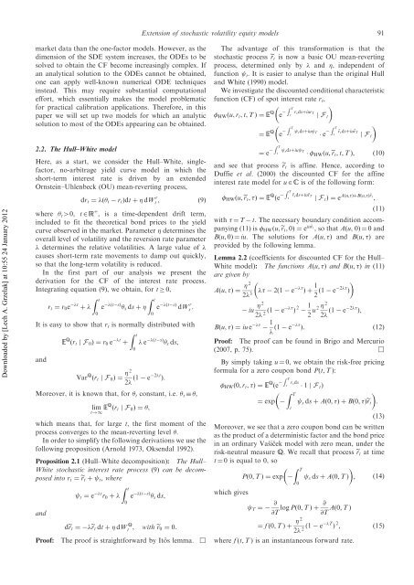
Extension of stochastic volatility equity models 91Downloaded by [Lech A. Grzelak] at 10:55 24 January 2012market data than the one-factor models. However, as thedimension of the SDE system increases, the ODEs to besolved to obtain the CF become increasingly complex. Ifan analytical solution to the ODEs cannot be obtained,one can apply well-known numerical ODE techniquesinstead. This may require substantial computationaleffort, which essentially makes the model problematicfor practical calibration applications. Therefore, in thispaper we will set up two models for which an analyticsolution to most of the ODEs appearing can be obtained.2.2. The Hull–White modelHere, as a start, we consider the Hull–White, singlefactor,no-arbitrage yield curve model in which theshort-term interest rate is driven by an extendedOrnstein–Uhlenbeck (OU) mean-reverting process,dr t ¼ ð t r t Þdt þ dW rt ,ð9Þwhere t 40, t 2 R þ , is a time-dependent drift term,included to fit the theoretical bond prices to the yieldcurve observed in the market. Parameter determines theoverall level of volatility and the reversion rate parameter determines the relative volatilities. A large value of causes short-term rate movements to damp out quickly,so that the long-term volatility is reduced.In the first part of our analysis we present thederivation for the CF of the interest rate process.Integrating equation (9), we obtain, for t 0,r t ¼ r 0 e t þ Z te ðt0sÞ s ds þ Z t0e ðt sÞ dW r s :It is easy to show that r t is normally distributed withandE Q ðr t jF 0 Þ¼r 0 e t þZ t0 e ðtsÞ s ds,Var Q ðr t jF 0 Þ¼ 22 ð1 e 2t Þ:Moreover, it is known that, for t constant, i.e. t ,limt!1 EQ ðr t jF 0 Þ¼,which means that, for large t, the first moment of theprocess converges to the mean-reverting level .In order to simplify the following derivations we use thefollowing proposition (Arnold 1973, Oksendal 1992).Proposition 2.1 (Hull–White decomposition): The Hull–White stochastic interest rate process (9) can be decomposedinto r t ¼ er t þ t , whereandProof:t ¼ e t r 0 þ Z te ðt0sÞ s ds,der t ¼ er t dt þ dW Q t , with er 0 ¼ 0:The proof is straightforward by Itoˆs lemma. œThe advantage of this transformation is that thestochastic process er t is now a basic OU mean-revertingprocess, determined only by and , independent offunction t . It is easier to analyse than the original Hulland White (1990) model.We investigate the discounted conditional characteristicfunction (CF) of spot interest rate r t ,R T HW ðu, r t , t, T Þ¼EeQ r s dsþiur Tt jF tR TR T¼ EeQ sdsþiu T ~rt es dsþiu~r Tt jF tR Ttsdsþiu¼ eT HW ðu,er t , t, T Þ, ð10Þand see that process er t is affine. Hence, according toDuffie et al. (2000) the discounted CF for the affineinterest rate model for u 2 C is of the following form:R Tt HW ðu,er t , Þ ¼E Q ~rðes dsþiu~r TjF t Þ¼e Aðu,ÞþBðu,Þ~r t,ð11Þwith ¼ T t. The necessary boundary condition accompanying(11) is HW ðu,er t ,0Þ¼e iu~r t, so that A(u, 0)¼ 0 andB(u,0)¼ iu. The solutions for A(u, ) and B(u, ) areprovided by the following lemma.Lemma 2.2 (coefficients for discounted CF for the Hull–White model): The functions A(u, ) and B(u, ) in (11)are given byAðu, Þ ¼ 2 2 3 2ð1 e Þþ 1 2 ð1 e 2 Þiu 22 2 ð1 e Þ 2 12 u 2 22 ð1 e 2 Þ,Bðu, Þ ¼iu e 1 ð1 e Þ: ð12ÞProof: The proof can be found in Brigo and Mercurio(2007, p. 75). œBy simply taking u ¼ 0, we obtain the risk-free pricingformula for a zero coupon bond P(t, T ): HW ð0, r t , Þ ¼E Q ðe¼ expR TtZ Ttr s ds 1 jF t Þs ds þ Að0, ÞþBð0, Þer tð13ÞMoreover, we see that a zero coupon bond can be writtenas the product of a deterministic factor and the bond pricein an ordinary Vasˇicˇek model with zero mean, under therisk-neutral measure Q. We recall that process er t at timet ¼ 0 is equal to 0, so Z TPð0, T Þ¼exps ds þ Að0, T Þ , ð14Þ0which gives@@T ¼ log Pð0, T Þþ@T @T Að0, T Þ¼ f ð0, T Þþ 22 2 ð1 e T Þ 2 , ð15Þwhere f (t, T ) is an instantaneous forward rate.:
92 L. A. Grzelak et al.Downloaded by [Lech A. Grzelak] at 10:55 24 January 2012This result shows that T can be obtained from theinitial forward curve, f(0, T ). The other time-invariantparameters, and , have to be estimated using marketprices of, in particular, interest rate caps. Now fromproposition 2.1 we have t ¼ (1/)(@/@t) t þ t , which reads t ¼ f ð0, tÞþ 1 2@ f ð0, tÞþ @t 2 2 ð1 e 2t Þ: ð16ÞMoreover, the CF, HW (u, r t , ), for the Hull–Whitemodel can be simply obtained by integration of s overthe interval [t, T ].2.3. Scho¨bel–Zhu–Hull–White hybrid modelIn this section we derive an analytic pricing formula in(semi-)closed form for European call options under theScho¨bel–Zhu–Hull–White (SZHW) asset pricing modelwith a full matrix of correlations, defined by (2). Thework on the SZHW hybrid model was initiated by Pelsser(Lord 2007) and resulted (later) in a working paper(Haastrecht et al. 2008).For the state vector X t ¼ [S t , r t , t ] T let us fixa probability space (, F, P) and a filtrationF¼{F t : t 0}, which satisfies the usual conditions.Furthermore, X t is assumed to be Markovian relative toF t . The Scho¨bel–Zhu–Hull–White hybrid model can beexpressed by the following 3D system of SDEs:dS t ¼ r t S t dt þ t S t dWt x dr t ¼ ð t r t Þdt þ dWt r ,d t ¼ ð t Þdt þ dWt , ð17Þwith the parameters as in equations (1), for p ¼ 1, and thecorrelationsdWt x dWt ¼ x, dt,dWtx dWt r ¼ x,r dt,dWt r dW t ¼ r, dt: ð18ÞBy extending the space vector (as in Cheng and Scaillet(2007)) with another stochastic process, defined byv t :¼ t 2,and choosing x t ¼ log S t , we obtain the following4D system of SDEs:1dx t ¼ er t þ t2 v tpdt þffiffiffiffiv tdWxt ,der t ¼ er t dt þ dW r t ,dv t ¼ð 2v t þ 2 t þ 2 pÞdt þ 2 ffiffiffiffi v t dWd t ¼ ð t Þdt þ dW t ,where we also used r t ¼ er t þ t , as in subsection 2.2. Notethat t is now included in t . We see that model (19) isindeed affine in the state vector X t ¼½x t ,er t , v t , t Š T . By theextension of the vector space we have obtained an affinemodel that enables us to apply the results from Duffieet al. (2000). In order to simplify the calculations, weintroduce a variable x t :¼ ex t þ t, where t ¼ R t0 s dsanddex t ¼ er t12 v t pffiffiffiffidt þ dWxv tt : ð19ÞB r ðu, Þ ¼ 1 ðiu 1Þð1 ð 2ÞÞ,B v ðu, Þ ¼ 1 4 2 1 ð 2d Þð d Þ,1 gð 2d ÞB ðu, Þ ¼f 0 f 1 þ 1 ðiu 1Þ x,r iu ðf 2 f 3 Þþ r,v2 ð d Þðf 4 þ f 5 Þ ,1 gð 2d Þ 1 1ð20Þ Aðu, Þ ¼f 6 log22g 1 2 3 f 7 þ ðu, Þ,According to Duffie et al. (2000) the discounted CF foru 2 C 4 is of the following form:R T SZHW ðu, X t , t, T Þ¼EeQ r s ds t e iuT X TjF t ð21ÞR Tsdsþiu¼ e½ T, T ,0,0Š TtR T EeQ ~r s dsþiu T X tTjF t ð22ÞR T¼ e tsdsþiu T ½ T, T ,0,0Š T e Aðu, ÞþBT ðu, ÞX t ,ð23ÞwhereX t ¼½ex t,er t , v t , t Š T ,Bðu, Þ ¼½B x ðu, Þ, B r ðu, Þ, B v ðu, Þ, B ðu, ÞŠ T :Now we set u ¼ [u,0,0,0] T , so that at time T we obtain theobvious boundary condition: SZHW ðu, X T , T, T Þ¼EQ ðe iuT X T jFT Þ¼e iuT X T ¼ eiu ~x T(as the price at time T is known deterministically). Thisboundary condition for ¼ 0 gives B x (u,0)¼ iu,A(u,0)¼ 0, B r (u,0)¼ 0, B (u,0)¼ 0 and B v (u,0)¼ 0. Thefollowing lemmas define the ODEs, from (8), and detailtheir solution.Lemma 2.3 (Scho¨bel–Zhu–Hull–White ODEs): Thefunctions A(u, ), B x (u, ), B (u, ), B v (u, ), B r (u, ) andu 2 R in (23) satisfy the following system of ODEs:dB xd ¼ 0,dB rd ¼ 1 þ B x B r ,dB vd ¼ 1 2 B xðB x 1Þþ2ð x,v B x ÞB v þ 2 2 Bv 2 ,dB d ¼ð2 B v þ x,r B x B r þ 2 r, v B r B v Þþð2 2 B v þ x, B x ÞB ,dAd ¼ 2 B v þ 1 2 2 Br 2 þ þ 1 2 2 B þ r B r B :Proof: The proof can be found in appendix A.1. œLemma 2.4: The solution to the system of ODEs specifiedin lemma 2.3 is given byt , B x ðu, Þ ¼iu,
Page 1 and 2: This article was downloaded by: [Le
Page 3: 90 L. A. Grzelak et al.Downloaded b
Page 7 and 8: 94 L. A. Grzelak et al.Downloaded b
Page 13 and 14: 100 L. A. Grzelak et al.10.9Strateg
Page 15 and 16: 102 L. A. Grzelak et al.Downloaded
Page 17 and 18: 104 L. A. Grzelak et al.Downloaded

Extension of stochastic volatility models with Hull-White interest rate ...

Create successful ePaper yourself

Delete template?

Save as template?