Extension of stochastic volatility models with Hull-White interest rate ...

This article was downloaded by: [Lech A. Grzelak]On: 24 January 2012, At: 10:55Publisher: RoutledgeInforma Ltd Registered in England and Wales Registered Number: 1072954 Registered office: MortimerHouse, 37-41 Mortimer Street, London W1T 3JH, UKQuantitative FinancePublication details, including instructions for authors and subscription information:http://www.tandfonline.com/loi/rquf20Extension of stochastic volatility equity models withthe Hull–White interest rate processLech A. Grzelak a b , Cornelis W. Oosterlee a c & Sacha Van Weeren ba Delft Institute of Applied Mathematics, Delft University of Technology, Mekelweg 4,2628 CD Delft, The Netherlandsb Derivatives Research and Validation Group, Rabobank, Jaarbeursplein 22, 3521 APUtrecht, The Netherlandsc CWI, National Research Institute for Mathematics and Computer Science, Kruislaan 413,1098 SJ Amsterdam, The NetherlandsAvailable online: 24 Jun 2011To cite this article: Lech A. Grzelak, Cornelis W. Oosterlee & Sacha Van Weeren (2012): Extension of stochastic volatilityequity models with the Hull–White interest rate process, Quantitative Finance, 12:1, 89-105To link to this article: http://dx.doi.org/10.1080/14697680903170809PLEASE SCROLL DOWN FOR ARTICLEFull terms and conditions of use: http://www.tandfonline.com/page/terms-and-conditionsThis article may be used for research, teaching, and private study purposes. Any substantial or systematicreproduction, redistribution, reselling, loan, sub-licensing, systematic supply, or distribution in any form toanyone is expressly forbidden.The publisher does not give any warranty express or implied or make any representation that the contentswill be complete or accurate or up to date. The accuracy of any instructions, formulae, and drug dosesshould be independently verified with primary sources. The publisher shall not be liable for any loss, actions,claims, proceedings, demand, or costs or damages whatsoever or howsoever caused arising directly orindirectly in connection with or arising out of the use of this material.

Quantitative Finance, Vol. 12, No. 1, January 2012, 89–105Extension of stochastic volatility equity models withthe Hull–White interest rate processLECH A. GRZELAK*yz, CORNELIS W. OOSTERLEEyx and SACHA VAN WEERENzDownloaded by [Lech A. Grzelak] at 10:55 24 January 20121. IntroductionyDelft Institute of Applied Mathematics, Delft University of Technology,Mekelweg 4, 2628 CD Delft, The NetherlandszDerivatives Research and Validation Group, Rabobank, Jaarbeursplein 22,3521 AP Utrecht, The NetherlandsxCWI, National Research Institute for Mathematics and Computer Science,Kruislaan 413, 1098 SJ Amsterdam, The Netherlands(Received 28 July 2008; in final form 6 July 2009)We present an extension of stochastic volatility equity models by a stochastic Hull–Whiteinterest rate component while assuming non-zero correlations between the underlyingprocesses. We place these systems of stochastic differential equations in the class of affinejump-diffusion–linear quadratic jump-diffusion processes so that the pricing of Europeanproducts can be efficiently performed within the Fourier cosine expansion pricing framework.We compare the new stochastic volatility Scho¨bel–Zhu–Hull–White hybrid model with aHeston–Hull–White model, and also apply the models to price hybrid structured derivativesthat combine the equity and interest rate asset classes.Keywords: Finance; Financial applications; Mathematical finance; Financial derivatives;Financial econometrics; Financial engineering; Mathematical models; Financial mathematicsIn recent years the financial world has focused on theaccurate pricing of exotic and hybrid products that arebased on a combination of underlyings from differentasset classes. In this paper we therefore present a flexiblemulti-factor stochastic volatility (SV) model that includesthe term structure of the stochastic interest rates (IR). Ouraim is to combine an arbitrage-free Hull–White IR modelin which the parameters are consistent with market pricesof caps and swaptions. In order to perform efficientoption valuation we fit this process in the class of affinejump-diffusion (AJD) processes (Duffie et al. 2000)(although jump processes are not included in this work).We specify under which conditions such a general modelcan fall in the class of AJD processes.A major step away from the assumption of constantvolatility in derivatives pricing was made by Hull andWhite (1990), Stein and Stein (1991) and Heston (1993),who defined the volatility as a diffusion process.This improved the pricing of derivatives under*Corresponding author. Email: l.a.grzelak@tudelft.nlheavy-tailed return distributions significantly and alloweda trader to quantify the uncertainty in the pricing.Stochastic volatility models have become popular forderivative pricing and hedging (see, for example, Fouqueet al. 2000), however financial engineers have developedmore complex exotic products that additionally requirethe modeling of a stochastic interest rate component. Aderivative pricing tool in which all these features areexplicitly modeled may have the potential of generatingmore accurate option prices for hybrid products. Theseproducts can be designed to provide capital or incomeprotection, diversification for portfolios and customizedsolutions for both institutional and retail markets.Fang and Oosterlee (2008a) developed a highly efficientalternative pricing method based on a Fourier-cosineexpansion of the density function and called it the COSmethod. This method can also determine a whole set ofoption prices in one computation. The COS algorithmrelies heavily on the availability of the characteristicfunction of the price process, which is guaranteed if westay within the AJD class (Duffie et al. 2000, Lewis 2001,Lee 2004). We examine the effect of correlated processesfor assets, stochastic volatility and interest rates on optionQuantitative FinanceISSN 1469–7688 print/ISSN 1469–7696 online ß 2012 Taylor & Francishttp://www.tandfonline.comhttp://dx.doi.org/10.1080/14697680903170809

90 L. A. Grzelak et al.Downloaded by [Lech A. Grzelak] at 10:55 24 January 2012prices through a comparison with, for example, the in which the squared volatility, v t ¼ t 2 , represents theHeston model.variance of the instantaneous stock return.pdS t ¼ rS t dt þffiffiffiffi v tStdW x t ,The dimension of the (complex-valued) ODEs for B(u, )dv t ¼ 2 v t þ t þ 2 dt þ 2ffiffiffifficorresponds to the dimension of the state vector, X t .pv t dWt2Typically, multi-factor models, such as the SZHW andthe HHW models, provide a better fit to the observedThe plan of the paper is as follows. In section 2 weperform an analysis of the Scho¨bel–Zhu–Hull–Whitemodel. In subsection 2.3 we show that the hybrid modelof interest admits a semi-closed form for the characteristicfunction. In the following subsection we derive theIt has already been reported by Heston (1993) andScho¨bel and Zhu (1999) that the plain Scho¨bel–Zhumodel is a particular case of the original Heston model.We can see that if ¼ 0, the Scho¨bel–Zhu model equalsthe Heston model in which H ¼ 2, H ¼ 2 =2, andHeston–Hull–White model with non-zero correlation H ¼ 2. This relation gives a direct connection betweenbetween the stock and the interest rate. In section 3 weshow how to efficiently price options with a Fouriercosinetheir discounted characteristic functions (Lord and Kahl2006). Finally, if we set r t constant and p ¼ 0 in the systemexpansion technique when the characteristic of equations (1), and zero correlations, the modelfunction with stochastic interest rate of the asset processis available. Further, in section 4 the two hybrid models,Scho¨bel–Zhu–Hull–White and Heston–Hull–White, andthe stochastic volatility Heston model are compared indetail with respect to calibration and hybrid productpricing. Section 5 concludes. The lengthy proofs of thecollapses to the standard Black–Scholes model.We will choose the parameters of equations (1) suchthat we deal with the Scho¨bel–Zhu–Hull–White (SZHW)model in subsection 2.3, and with the Heston–Hull–White(HHW) model in subsection 2.4. Gaspar (2004) andCheng and Scaillet (2007) showed that the so-calledlemmas are given in the appendices.linear-quadratic jump-diffusion (LQJD) models areequivalent to the AJD models with an augmented statevector.2. Extension of stochastic volatility equity models2.1. Affine jump-diffusion processesIn this section we present a hybrid stochastic volatilityThe AJD class refers to a fixed probability space (, F, P)equity model that includes a stochastic interest rateand a Markovian n-dimensional affine process X t in someprocess. In particular, we add to the SV model the wellknownHull–White stochastic interest rate process (Hullspace D R n . The model without jumps can be expressedby the following stochastic differential form:and White 1996), which is a generalization of the Vasˇicˇek(1977) model.dX t ¼ ðX t Þdt þ ðX t ÞdW t ,We consider a three-dimensional system of stochastic where W t is a F t -standard Brownian motion in R n , (X t ):differential equations of the formD ! R n , (X t ):D ! R nn . Moreover, for processes indS t ¼ r t S t dt þ t p S t dWt x ,the AJD class it is assumed that drift (X t ), volatilitydr t ¼ ð t r t Þdt þ dWt r (X t )(X t ) T and interest rate component r(X t ) are of theaffine form, i.e.d t ¼ ð t Þdt þ t1 p dW t , ð1Þ ðX t Þ¼a 0 þ a 1 X t , for any ða 0 , a 1 Þ2R n R nn , ð5Þwhere p is an exponent, and control the speed ofmean reversion, represents the interest rate volatility, ðX t ÞðX t Þ T ¼ðc 0 Þ ij þðc 1 Þ T ij X t, for arbitraryand 1 p determines the variance of the t process.Parameters and t are the long-run mean of theðc 0 , c 1 Þ2R nn R nnn , ð6Þvolatility and the interest rate processes, respectively.W i are correlated Wiener processes, also governed byrðX t Þ¼r 0 þ r T 1 X t, for ðr 0 , r 1 Þ2R R n : ð7Þan instantaneous covariance matrix,Then, for a state vector, X t , the discounted characteristic23function (CF) is of the following form:1 x, x,rR67T ¼ 4 ,x 1 ,r 5dt:ð2Þ ðu, X t , t, T Þ¼E Q rðes dsþiu T X Tt jF t Þ¼e Aðu, ÞþBT ðu, ÞX t, r,x r, 1where the expectation is taken under the risk-neutralIf we keep r t deterministic and p ¼ 1/2, we have the measure, Q. For a time lag, :¼ T t, the coefficientsHeston (1993) model,A(u, ) and B T (u, ) have to satisfy certain complex-valuedpdS t ¼ rS t dt þffiffiffiffi tStdW x t ,ordinary differential equations (ODEs) (Duffie et al.d t ¼ H ð H t Þdt þ H p ffiffiffiffi2000): t dWt : ð3ÞdFor p ¼ 1, our model is, in fact, the generalized Stein–d Aðu, Þ ¼ r 0 þ B T a 0 þ 1 2 BT c 0 B,Stein (Stein and Stein 1991) model, which is also calleddthe Scho¨bel–Zhu (Scho¨bel and Zhu 1999) model,d Bðu, Þ ¼ r 1 þ a T 1 B þ 1 ð8Þ2 BT c 1 B:

Extension of stochastic volatility equity models 91Downloaded by [Lech A. Grzelak] at 10:55 24 January 2012market data than the one-factor models. However, as thedimension of the SDE system increases, the ODEs to besolved to obtain the CF become increasingly complex. Ifan analytical solution to the ODEs cannot be obtained,one can apply well-known numerical ODE techniquesinstead. This may require substantial computationaleffort, which essentially makes the model problematicfor practical calibration applications. Therefore, in thispaper we will set up two models for which an analyticsolution to most of the ODEs appearing can be obtained.2.2. The Hull–White modelHere, as a start, we consider the Hull–White, singlefactor,no-arbitrage yield curve model in which theshort-term interest rate is driven by an extendedOrnstein–Uhlenbeck (OU) mean-reverting process,dr t ¼ ð t r t Þdt þ dW rt ,ð9Þwhere t 40, t 2 R þ , is a time-dependent drift term,included to fit the theoretical bond prices to the yieldcurve observed in the market. Parameter determines theoverall level of volatility and the reversion rate parameter determines the relative volatilities. A large value of causes short-term rate movements to damp out quickly,so that the long-term volatility is reduced.In the first part of our analysis we present thederivation for the CF of the interest rate process.Integrating equation (9), we obtain, for t 0,r t ¼ r 0 e t þ Z te ðt0sÞ s ds þ Z t0e ðt sÞ dW r s :It is easy to show that r t is normally distributed withandE Q ðr t jF 0 Þ¼r 0 e t þZ t0 e ðtsÞ s ds,Var Q ðr t jF 0 Þ¼ 22 ð1 e 2t Þ:Moreover, it is known that, for t constant, i.e. t ,limt!1 EQ ðr t jF 0 Þ¼,which means that, for large t, the first moment of theprocess converges to the mean-reverting level .In order to simplify the following derivations we use thefollowing proposition (Arnold 1973, Oksendal 1992).Proposition 2.1 (Hull–White decomposition): The Hull–White stochastic interest rate process (9) can be decomposedinto r t ¼ er t þ t , whereandProof:t ¼ e t r 0 þ Z te ðt0sÞ s ds,der t ¼ er t dt þ dW Q t , with er 0 ¼ 0:The proof is straightforward by Itoˆs lemma. œThe advantage of this transformation is that thestochastic process er t is now a basic OU mean-revertingprocess, determined only by and , independent offunction t . It is easier to analyse than the original Hulland White (1990) model.We investigate the discounted conditional characteristicfunction (CF) of spot interest rate r t ,R T HW ðu, r t , t, T Þ¼EeQ r s dsþiur Tt jF tR TR T¼ EeQ sdsþiu T ~rt es dsþiu~r Tt jF tR Ttsdsþiu¼ eT HW ðu,er t , t, T Þ, ð10Þand see that process er t is affine. Hence, according toDuffie et al. (2000) the discounted CF for the affineinterest rate model for u 2 C is of the following form:R Tt HW ðu,er t , Þ ¼E Q ~rðes dsþiu~r TjF t Þ¼e Aðu,ÞþBðu,Þ~r t,ð11Þwith ¼ T t. The necessary boundary condition accompanying(11) is HW ðu,er t ,0Þ¼e iu~r t, so that A(u, 0)¼ 0 andB(u,0)¼ iu. The solutions for A(u, ) and B(u, ) areprovided by the following lemma.Lemma 2.2 (coefficients for discounted CF for the Hull–White model): The functions A(u, ) and B(u, ) in (11)are given byAðu, Þ ¼ 2 2 3 2ð1 e Þþ 1 2 ð1 e 2 Þiu 22 2 ð1 e Þ 2 12 u 2 22 ð1 e 2 Þ,Bðu, Þ ¼iu e 1 ð1 e Þ: ð12ÞProof: The proof can be found in Brigo and Mercurio(2007, p. 75). œBy simply taking u ¼ 0, we obtain the risk-free pricingformula for a zero coupon bond P(t, T ): HW ð0, r t , Þ ¼E Q ðe¼ expR TtZ Ttr s ds 1 jF t Þs ds þ Að0, ÞþBð0, Þer tð13ÞMoreover, we see that a zero coupon bond can be writtenas the product of a deterministic factor and the bond pricein an ordinary Vasˇicˇek model with zero mean, under therisk-neutral measure Q. We recall that process er t at timet ¼ 0 is equal to 0, so Z TPð0, T Þ¼exps ds þ Að0, T Þ , ð14Þ0which gives@@T ¼ log Pð0, T Þþ@T @T Að0, T Þ¼ f ð0, T Þþ 22 2 ð1 e T Þ 2 , ð15Þwhere f (t, T ) is an instantaneous forward rate.:

92 L. A. Grzelak et al.Downloaded by [Lech A. Grzelak] at 10:55 24 January 2012This result shows that T can be obtained from theinitial forward curve, f(0, T ). The other time-invariantparameters, and , have to be estimated using marketprices of, in particular, interest rate caps. Now fromproposition 2.1 we have t ¼ (1/)(@/@t) t þ t , which reads t ¼ f ð0, tÞþ 1 2@ f ð0, tÞþ @t 2 2 ð1 e 2t Þ: ð16ÞMoreover, the CF, HW (u, r t , ), for the Hull–Whitemodel can be simply obtained by integration of s overthe interval [t, T ].2.3. Scho¨bel–Zhu–Hull–White hybrid modelIn this section we derive an analytic pricing formula in(semi-)closed form for European call options under theScho¨bel–Zhu–Hull–White (SZHW) asset pricing modelwith a full matrix of correlations, defined by (2). Thework on the SZHW hybrid model was initiated by Pelsser(Lord 2007) and resulted (later) in a working paper(Haastrecht et al. 2008).For the state vector X t ¼ [S t , r t , t ] T let us fixa probability space (, F, P) and a filtrationF¼{F t : t 0}, which satisfies the usual conditions.Furthermore, X t is assumed to be Markovian relative toF t . The Scho¨bel–Zhu–Hull–White hybrid model can beexpressed by the following 3D system of SDEs:dS t ¼ r t S t dt þ t S t dWt x dr t ¼ ð t r t Þdt þ dWt r ,d t ¼ ð t Þdt þ dWt , ð17Þwith the parameters as in equations (1), for p ¼ 1, and thecorrelationsdWt x dWt ¼ x, dt,dWtx dWt r ¼ x,r dt,dWt r dW t ¼ r, dt: ð18ÞBy extending the space vector (as in Cheng and Scaillet(2007)) with another stochastic process, defined byv t :¼ t 2,and choosing x t ¼ log S t , we obtain the following4D system of SDEs:1dx t ¼ er t þ t2 v tpdt þffiffiffiffiv tdWxt ,der t ¼ er t dt þ dW r t ,dv t ¼ð 2v t þ 2 t þ 2 pÞdt þ 2 ffiffiffiffi v t dWd t ¼ ð t Þdt þ dW t ,where we also used r t ¼ er t þ t , as in subsection 2.2. Notethat t is now included in t . We see that model (19) isindeed affine in the state vector X t ¼½x t ,er t , v t , t Š T . By theextension of the vector space we have obtained an affinemodel that enables us to apply the results from Duffieet al. (2000). In order to simplify the calculations, weintroduce a variable x t :¼ ex t þ t, where t ¼ R t0 s dsanddex t ¼ er t12 v t pffiffiffiffidt þ dWxv tt : ð19ÞB r ðu, Þ ¼ 1 ðiu 1Þð1 ð 2ÞÞ,B v ðu, Þ ¼ 1 4 2 1 ð 2d Þð d Þ,1 gð 2d ÞB ðu, Þ ¼f 0 f 1 þ 1 ðiu 1Þ x,r iu ðf 2 f 3 Þþ r,v2 ð d Þðf 4 þ f 5 Þ ,1 gð 2d Þ 1 1ð20Þ Aðu, Þ ¼f 6 log22g 1 2 3 f 7 þ ðu, Þ,According to Duffie et al. (2000) the discounted CF foru 2 C 4 is of the following form:R T SZHW ðu, X t , t, T Þ¼EeQ r s ds t e iuT X TjF t ð21ÞR Tsdsþiu¼ e½ T, T ,0,0Š TtR T EeQ ~r s dsþiu T X tTjF t ð22ÞR T¼ e tsdsþiu T ½ T, T ,0,0Š T e Aðu, ÞþBT ðu, ÞX t ,ð23ÞwhereX t ¼½ex t,er t , v t , t Š T ,Bðu, Þ ¼½B x ðu, Þ, B r ðu, Þ, B v ðu, Þ, B ðu, ÞŠ T :Now we set u ¼ [u,0,0,0] T , so that at time T we obtain theobvious boundary condition: SZHW ðu, X T , T, T Þ¼EQ ðe iuT X T jFT Þ¼e iuT X T ¼ eiu ~x T(as the price at time T is known deterministically). Thisboundary condition for ¼ 0 gives B x (u,0)¼ iu,A(u,0)¼ 0, B r (u,0)¼ 0, B (u,0)¼ 0 and B v (u,0)¼ 0. Thefollowing lemmas define the ODEs, from (8), and detailtheir solution.Lemma 2.3 (Scho¨bel–Zhu–Hull–White ODEs): Thefunctions A(u, ), B x (u, ), B (u, ), B v (u, ), B r (u, ) andu 2 R in (23) satisfy the following system of ODEs:dB xd ¼ 0,dB rd ¼ 1 þ B x B r ,dB vd ¼ 1 2 B xðB x 1Þþ2ð x,v B x ÞB v þ 2 2 Bv 2 ,dB d ¼ð2 B v þ x,r B x B r þ 2 r, v B r B v Þþð2 2 B v þ x, B x ÞB ,dAd ¼ 2 B v þ 1 2 2 Br 2 þ þ 1 2 2 B þ r B r B :Proof: The proof can be found in appendix A.1. œLemma 2.4: The solution to the system of ODEs specifiedin lemma 2.3 is given byt , B x ðu, Þ ¼iu,

Extension of stochastic volatility equity models 93Downloaded by [Lech A. Grzelak] at 10:55 24 January 2012whereðu, Þ¼withZ 0B ðu, sÞ þ 1 2 2 B ðu, sÞþ r, B r ðu, sÞ ds,f 0 ¼ðd Þð2d Þ g , 16 f 1 ¼4 2 d ð d Þsinh 2 d,4f 2 ¼ 2 ðððd Þ 1Þþgðð d Þ 1ÞÞ,d2ððd 2Þ 1Þ2gð1 ð2 d ÞÞ,d þ 2f 3 ¼d 2f 4 ¼ 2 4d 2 d þ 2d þ 2 ,22ð2df 5 ¼ ð 2 d Þ ð2Þð1 þ ð2d ÞÞdf 6 ¼ 14 2 ð d Þ,f 7 ¼ðiu 1Þ 2 ð3 þ ð 4Þ 4ð 2Þ 2Þ,Þd 2ð24Þ2,d þ 2pand ¼ 2( x,v ui), d ¼ ffiffiffiffiffiffiffiffiffiffiffiffiffiffiffiffiffiffiffiffiffi 2 8 2 , with ¼12uði þ uÞ, g ¼ ( d)/( þ d) and (x) ¼ exp(x/2).Proof: The proof is presented in appendix A.2. œNow, since we have found expressions for the coefficientsA(u, ) and B T (u, ) we return to equation (21) andderive a representation in which the term structure isincluded. It is known that the price of a zero coupon bondcan be obtained from the characteristic function by takingu ¼ [0, 0, 0, 0] T . So, Z T SZHW ð0, X t , Þ ¼exps ds SZHW ð0, X t , Þ:Since er 0 ¼ 0 we find Z TPð0, T Þ¼exp0ts ds þ Að0, ÞþB x ð0, Þx 0þ B v ð0, Þv 0 þ B ð0, Þ 0,ð25Þwith boundary conditions B x (0, T ) ¼ 0, B v (0, T ) ¼ 0,B (0, T ) ¼ 0 andAð0, T Þ¼ 1 Z T2 2 B r ð0, sÞ 2 ds ¼ 2We thus find0Pð0, T Þ¼expZ T04 3 ð1 þ 2T ðe T 2Þ 2 Þ:s ds þ Að0, T Þ :ð26ÞBy combining the results from the previous lemmas, wecan prove the following lemma.Lemma 2.5: In the Scho¨bel–Zhu–Hull–White model, thediscounted characteristic function, SZHW (u, X t , t, T ) forlog S T , is given by SZHW ðu, X t , t, T Þ¼expðeAðu, ÞþB x ðu, Þx t þ B r ðu, Þ~r tþ B v ðu, Þv t þ B ðu, Þ t Þ,where B x (u, ), B r (u, ), B v (u, ), B (u, ) and A(u, ) aregiven in lemma 2.4, andZ TeAðu, Þ ¼Aðu, Þþðiu 1Þ s ds ¼ Aðu, Þþðu, t, T Þ,tð27Þwithðu,t,TÞ¼ð1 iuÞ logPð0,TÞ þ 2 þ 2 Tðe e t ÞPð0,tÞ 2 2 1 2Tðe e 2t Þ : ð28Þ2Proof: The proof is straightforward from the definitionof the discounted CF.œ2.3.1. Numerical integration for the SZHW hybridmodel. Lemma 2.4 indicates that many terms in theCF for the SZHW hybrid model can be obtainedanalytically, except the (u, ) term (24), which requiresnumerical integration of the hyper-geometric function 2 F 1(Mayrhofer and Fischer 1996). For a given partitioning0 ¼ s 1 s 2 s N 0 1 s N 0 ¼ ,we calculate the following integral approximation of (24):ðu,Þ XN0B ðu,s i Þ þ 1 2 2 B ðu,s i Þþ r, B r ðu,s i Þ si ,i¼0ð29Þwith the functions B r (u, s i ) and B (u, s i ) as in (24). In table 1we present the numerical convergence results for two basicquadrature rules for one particular (representative) exampleof (29). It shows that both integration routines—thecomposite trapezoidal and the composite Simpson rule—converge very satisfactory with only a small number of gridpoints, N 0 . Convergence with the trapezoidal rule is ofTable 1. CPU time, absolute error, and the convergence ratefor different numbers of integration points N 0 for evaluatingfunction (u, ). The time to maturity is set to ¼ 1 and u ¼ 5and the remaining parameters for the model are ¼ 0.5, ¼ 1, ¼ 0.1, ¼ 0:3, ¼ 0.5, x,v ¼ 0.5, x,r ¼ 0.3, r 0 ¼ 0.05, 0 ¼ 0.256 and r,v ¼ 0.9.(N 0 ¼ 2 n0 )Trapezoidal ruleSimpson’s rulen 0 Time (s) jErrorj Time (s) jErrorj2 1.5e 4 1.5e 4 1.5e 4 7.3e 64 2.6e 4 6.0e 6 2.7e 4 2.3e 86 3.4e 4 3.4e 7 3.5e 4 1.3e 108 6.6e 4 2.1e 8 6.7e 4 6.0e 13

94 L. A. Grzelak et al.Downloaded by [Lech A. Grzelak] at 10:55 24 January 2012second order, and with Simpson’s rule of fourth order, asexpected. Simpson’s rule is superior in terms of the ratiobetween time and absolute error. We therefore continuewith the Simpson rule, setting N 0 ¼ 2 6 .2.4. Heston–Hull–White hybrid modelIt is known, for example from Muskulus et al. (2007), thatit is not possible to formulate the so-called Heston–Hull–White (HHW) hybrid process, with a full matrix ofcorrelations, so that it belongs to the class of AJDprocesses. For this, restrictions regarding the parametersor the correlation structure have to be introduced. Onepossible restriction is to assume that the interest rateprocess, r t , evolves independently of the stock price, S t ,and the volatility process, t , while the other correlationis not equal to zero, i.e. dW x t dW r t ¼ 0, dW t dW rt ¼ 0and dW x t dW t ¼ x, dt. Another option is to solve theproblem under the assumption that dW t dW rt ¼ 0 and,additionally, that 2 =4 ¼ (Muskulus et al. 2007). Itmay, however, be difficult to apply this latter model inpractice, as the economical meaning of the parameterrelationship is difficult to interpret.Since for the HHW model with a full matrix ofcorrelations between the processes the affinity of themodel is lost, the aim is to reformulate the HHW modelso that affinity is preserved while the correlations areincluded to some extent. Giese (2006) introduced thefollowing HHW-type model:pdS t ¼ r t S t dt þffiffiffiffi tStdW xt þ S, r S t dW r t ,dr t ¼ ð t r t Þdt þ dW rt ,pd t ¼ ð t Þdt þ ffiffiffiffi t dWt ,ð30ÞwithdW x tdW x t dW t dW rt ¼ 0,¼ x, dt,dW rt dW t ¼ 0: ð31ÞSince the interest rate, r t , is uncorrelated with the otherdriving processes, the reformulated HHW model stays(in the log-space for equity) in the class of affineprocesses. By taking S,r ¼ 0 the model collapses to thewell-known Heston–Hull–White model with independentinterest rate. We see that by S,r 6¼ 0 one controls,indirectly, the correlation between the equity and interestrate processes.Now, by log-transform of the stock process, x t ¼ log S t ,and using r t ¼ er t þ t and x t ¼ ex t þ t, we obtain1dex t ¼ er t 2 ð t þ S,r 2 Þ pdt þffiffiffiffi tder t ¼ er t dt þ dW rt ,pd t ¼ ð t Þdt þ ffiffiffiffi t dWt :dWxtþ S,r dW rt ,ð32Þdiscounted CF. Since for constant S,r the system isalready affine, the CF for u 2 C 3 is of the following form:R T HHW ðu, X t , t, T Þ¼EeQ r s ds t e iuT X TjF t ð33Þ¼ eR Ttsdsþiu T ½ T, T ,0Š T e Aðu, ÞþBT ðu, ÞX t ,ð34Þwhere X t ¼½ex t,er t , t Š T and B(u, ) ¼ [B x (u, ), B r (u, ),B (u, )] T . As before, by setting u ¼ [u,0,0] T we find thecorresponding ODEs and their solutions.Lemma 2.6 (Heston–Hull–White ODEs): The functionsA(u, ), B x (u, ), B r (u, ) and B (u, ), u 2 R, in (33) satisfythe following system of ODEs:dB xd ¼ 0,dB rd ¼ 1 þ B x B r ,dB d ¼ 1 2 B xðB x 1Þþð x, B x ÞB þ 1 2 2 B 2 ,dAd ¼ 1 2 S,r 2 B xðB x 1Þþ S,r B x B r þ 1 2 2 Br 2 þ B ,with boundary conditions B x (u,0)¼ iu, B (u,0)¼ 0,B r (u,0)¼ 0 and A(u,0)¼ 0.Proof: The proof can be found in appendix A.3. œLemma 2.7 (CF coefficients for the HHW model): Thesolution to the system of ODEs specified in lemma 2.4 isgiven byB x ðu, Þ ¼iu,B r ðu, Þ ¼ 1 ðiu 1Þð1 ð 2ÞÞ,B ðu, Þ ¼ 1 1 ð 2d Þ ð d Þ,21 gð 2d ÞAðu, Þ ¼ ð 4Þ dgð 1 ðÞþð4Þ 2 ðÞÞ2dggð 2d Þ 1þ 3 ðÞ log ,g 1where1ðÞ ¼ f 4 f6 2 þ 2f 6ð f 3 þ 2f 4 f 6 Þð2Þ,2ðÞ ¼ð f 6 ð2f 3 þ 3f 4 f 6 Þþ2ð f 1 þ f 2 f 5 þ f 6 ð f 3 þ f 4 f 6 ÞÞÞ,3ðÞ ¼2f 2 f 5 ð4Þðg 1Þ,with f 1 ¼ 1 2 S,r 2 uði þ uÞ, f 2 ¼ , f 3 ¼ S,r iu, f 4 ¼ 1 2 2 ,pf 5 ¼ (1/ 2 )( d ), f 6 ¼ (1/)(iu 1), d ¼ ffiffiffiffiffiffiffiffiffiffiffiffiffiffiffiffiffiffiffiffiffiffiffiffiffiffiffiffiffiffiffiffi 2 þðiu þ u 2 Þ 2 ,g ¼ ( d )/( þ d ), ¼ x, iu and (x) ¼ exp(x/2).Proof: The proof requires solving Riccati-type ODEsthat are analogous to those for the SZHW hybridmodel.œNow, by the above lemma the CF for the HHW hybridmodel in (33) for log S t is given byAs in the case of the SZHW hybrid model, the nextstep of the analysis is to find the corresponding HHW ðu, X t , t, T Þ¼expðeAðu, ÞþB x ðu, Þx tþ B r ðu, Þ~r t þ B ðu, Þ t Þ,ð35Þ

Extension of stochastic volatility equity models 95Downloaded by [Lech A. Grzelak] at 10:55 24 January 2012whereeAðu, Þ ¼Aðu, Þþðu, t, T Þ,where B x (u, ), B r (u, ), B (u, ) and A(u, ) are given inlemma 2.7, and W(u, t, T ) is given in equation (28).As already mentioned, the HHW model defined in (30)assumes a zero correlation between the equity process S tand the short-term r t , i.e. dW x t dW r t ¼ 0, as these twoprocesses are indirectly linked via S,r . We now discussthe relation between S,r and the instantaneous correlation x,r .By Itoˆ’s lemma and dW xtinstantaneous correlation dW rt ¼ 0 we have theCovðdS t ,dr t Þ x,r ¼ pffiffiffiffiffiffiffiffiffiffiffiffiffiffiffiffiffiffipffiffiffiffiffiffiffiffiffiffiffiffiffiffiffiffiffiVarðdS t Þ Varðdr t Þ S,r S t dt S,r¼ qffiffiffiffiffiffiffiffiffiffiffiffiffiffiffiffiffiffiffiffiffiffiffiffiffiffiffiffiffiffiffiffiffiffiffiffiffiffiffi t St 2 dt þ s, 2 r S t 2 dtpffiffiffiffiffiffiffiffiffiffi¼ q ffiffiffiffiffiffiffiffiffiffiffiffiffiffiffiffiffiffi : ð36Þ 2 dt t þ S,r2From (36) we find S,r as a function of x,r : S,r ðtÞ ¼ pffiffiffiffix,r tq ffiffiffiffiffiffiffiffiffiffiffiffiffiffiffi :1 x,r2Since S,r is defined in terms of the stochastic process t ,it is also stochastic. The first approach to deal with statedependent S,r is to include it in the original system (30);however, the system’s affinity may then become problematic.In this article we therefore adopt the basicapproximation for S,r proposed by Giese (2006), i.e.qffiffiffiffiffiffiffiffiffiffiffiffiffiffiffiffiffiffiffiffiffiffiffiffiffiffiffiffi x,r E ð1=T Þ R T0 t dt S,r q ffiffiffiffiffiffiffiffiffiffiffiffiffiffiffi , ð37Þ1 x,r2which can be further simplifiedy via0sffiffiffiffiffiffiffiffiffiffiffiffiffiffiffiffiffiffiffiffi1Z1 TE@ t dsA E 1 Z T t dsTT001 Varð R T4T0 t dsÞEð R T0 t dsÞ! 1=2:ð38ÞSince t is a Cox–Ingersoll–Ross (CIR)-type process theexpectations and variance on the RHS of (38) can befound analytically.2.4.1. Limits for the HHW hybrid model. We analysehere the accuracy of the approximation for S,rintroduced in (37). With a prescribed correlation, x,r ,we approximate the effective S,r in equation (37) andcompare it with the correlation, e S,r , obtained by a MonteCarlo simulation of (30). The results are generated by50,000 Monte Carlo paths with a step-size of 0.01.Table 2 shows that, although the instantaneous correlationbetween the equity process and the interest rate canbe indirectly included in the HHW model via S,r , someextreme correlations cannot be generated. Moreover,Table 2. The error for instantaneous correlation, by a MonteCarlo simulation. The simulation is performed with ¼ 0.35, ¼ 0:05, ¼ 0.4, ¼ 0.15, ¼ 0.07, x, ¼ 0.7, S 0 ¼ 1,v 0 ¼ 0.0625 and r 0 ¼ 0.02.Maturity x,r (%) S,r e S;r (%) x;r e x;r (%) ¼ 2 30 0.0646 29.90 0.10050 0.1187 48.84 1.16070 0.2016 66.90 3.10090 0.4247 79.23 10.77 ¼ 12 30 0.0587 25.25 4.75050 0.1078 38.85 11.1570 0.1831 45.89 24.1190 0.3857 41.16 48.81we also see that this effect is more pronounced forlong maturities. Thus, we cannot fully control the HHWmodel, as accurate calibration and pricing, especially forhigh correlations and long maturities, is not guaranteed.Often in practice, however, we hardly encounter such highcorrelations. However, since this model admits a closedform for the CF, we do not need a numerical integrationprocedure as in section 2.3.1 for SZHW.3. Pricing methodologyThe pricing of plain vanilla options is common practice inthe Fourier domain when the CF of the logarithm of thestock price is available.Recently, an effective pricing method, the COS method,based on Fourier-cosine expansion, was developed byFang and Oosterlee (2008a). This method can also (as theCarr–Madan method (Carr and Madan 1999)) computethe option prices for a whole strip of strikes in onecomputation and also depends on the availability ofthe CF. Implementation is straightforward. The COSmethod can achieve an exponential convergence rate forEuropean, Bermudan and barrier options for affinemodels whose probability density function is in C 1 [a, b],with non-zero derivatives (Fang and Oosterlee 2008a, b).Here, we extend the COS method to include thestochastic interest rate process.We start the description of the pricing method with thegeneral risk-neutral pricing formula: R TVðt, S t Þ¼E Q res ds t VðT, S T ÞjF tZ¼ VðT, yÞ b f Y ðy j xÞdy,ð39ÞRwhere b f Y ð y j xÞ ¼ R R ez f Y, Z ð y, z j xÞdz, with z ¼tr s ds.The claim V(t, S t ) under E Q () is defined in S t whichmay be correlated to r t . As we assume a fast decay of thedensity function, the following approximation can bemade:ZVðt, S t Þ VðT, yÞ b f Y ðy j xÞdy, ð40ÞR Tyvar( f(X )) ( f 0 (E(X ))) 2 var(X ).

96 L. A. Grzelak et al.Downloaded by [Lech A. Grzelak] at 10:55 24 January 2012where ¼ [ 1 , 2 ] and jj¼ 2CF is now given by 1 , 2 4 1 . The discountedðu, X t , t, T Þ¼E Q rðes dsþiu T X Tt jF t Þ, ð41Þwhich, for u ¼ [u,0,...,0] T and X T ¼ [S T , r T , ...] T , readsZZZðu,X t ,t,TÞ¼ e zþiuy f Y,Z ðy,z j xÞdzdy ¼ e iuy b fY ðy j xÞdy:RRð42ÞNote that the integration in (42) is simply the Fouriertransform of b f Y ð yjxÞ, which can be approximated on abounded domain ,Zðu, X t , t, T Þ e iuy b f Y ð y j xÞdy ¼: ~ðu, X t , t, T Þ:ð43ÞSince we are interested in the pricing of claims of the form(40), we link b f Y ð yjxÞ with its CF via the following result.Result 3.1: For a given bounded domain ¼ [ 1 , 2 ], andN a number of terms in the expansion, the probabilitydensity function b f Y ð yjxÞ given by (40) can be approximatedbyb fY ð yjxÞ XN n cos np ðy 1Þ,jjn¼0where n ¼ 2! njj < ~ np exp np i 1,jj jjwhere R denotes taking the real part, ! 0 ¼ 1 2 and ! n ¼ 1,n 2 N þ .For a proof we refer to the original paper on the COSmethod (Fang and Oosterlee 2008a).Using the above lemma, we replace the probabilitydensity function b f Y ð yjxÞ in (40),ZVðt, S t Þ VðT, yÞ XN n cos np ð y 1Þdyjjn¼0¼ jj X N n n, ð44Þ2 !n¼0 nwheren ¼ 2! ZnVðT, yÞ cos np ð y 1Þdy: ð45Þjj jjThe above equation provides us with the pricing formulafor any stochastically discounted payoff, V(T, S T ), forwhich the CF is available. We note that, depending onthe payoff, the n in (45) change, but a closed-formexpression is available for the most common payoffs.As the hybrid products will be calibrated to plain vanillaoptions, we provide the gamma coefficients for theEuropean call options.Result 3.2: The n coefficient in (45) for pricing a calloption defined byVðT, yÞ ¼maxðKðe y 1Þ,0Þ,R Twith y ¼ log(S/K ) for a given strike K, is given byn ¼ 2Kjj ð n n Þ, ð46Þwherejj 2 n ¼jj 2 þðnpÞ 2 cosðnpÞe 21 npcos þ npjj jj sinðnpÞe 2 1 npsin, ð47Þjjand( h ijjn ¼np sinðnpÞ sin 1 npjj, for n 6¼ 0,ð48Þ 2 , for n ¼ 0:Proof: The proof is straightforward by calculating theintegral in (45) with the transformed payoff functionV(T, y).œSince the coefficients n are available in closed form,the expression in (44) can easily be implemented.The availability of such a pricing formula is particularlyuseful in a calibration procedure, in which the parametersof the stochastic processes need to be approximated.In practice, option pricing models are calibrated to anumber of market observed call option prices. It istherefore necessary for such a procedure to be highlyefficient and a (semi-)closed form for an option pricingformula is desirable.The COS method’s accuracy is related to the size of theintegration domain, . If the domain is chosen too small,we expect a significant loss of accuracy (Fang andOosterlee 2008a). On the other hand, if the domain istoo wide, a large number of terms in the Fourierexpansion, N, has to be used for satisfactory accuracy.Fang and Oosterlee (2008a) defined the truncation rangein terms of the moments of log(S T /K) of the formqffiffiffiffiffiffiffiffiffiffiffiffiffiffiffiffiffiffiffiffip 1,2 ¼ 1 L 2 þffiffiffiffiffi , ð49Þwith the minus sign for 1 and the plus sign for 2 , the i are the corresponding ith moments, and L is anappropriate constant. In our work, with the moments notdirectly available, we apply a simplified approximationfor the integration range, and usep 1,2 ¼ 0 Lffiffi ,ð50Þwith the time to maturity. As in Fang and Oosterlee(2008a), we fix L ¼ 8 in (50).4. Calibration and pricing under the hybrid modelFor exotic financial products that involve more than oneasset class, the pricing engine should be based on astochastic model that takes into account the interactionsbetween the asset classes, such as the SZHW and HHWmodels presented above. It is therefore interesting toevaluate price differences between the classical modelsand these hybrid models. For this purpose we considerseveral hybrid products, treated in subsequent subsections.The pricing is done using a Monte Carlo method. 4

Extension of stochastic volatility equity models 97Downloaded by [Lech A. Grzelak] at 10:55 24 January 2012Before we can price these products, however, we needto calibrate the models, i.e. to find the model parametersso that the models recover the market prices of plainvanilla options. This calibration procedure relies heavilyon the characteristic function derived in the previoussection and the appendices.4.1. Calibration of the modelsIn this section we examine the extended stochasticvolatility models and compare their performance withthe Heston model. We use financial market data toestimate the model parameters and discuss the effect ofthe correlation between the equity and interest rate onthe estimated parameters. For this purpose we have chosenthe CAC40 call option implied volatilities of 17.10.2007.We perform the calibration of the models in two stages.Firstly, we calibrate the parameters for the interest rateprocess using caplets and swaptions. Secondly, theremaining parameters, for the underlying asset, thevolatility and the correlations, are calibrated to the plainvanilla option market prices. Standard procedures for theHull–White calibration are employed (Brigo and Mercurio2007). Tables 3 and 4 present the estimated parameters andthe associated squared sum errors (SSE), defined asSSE ¼ Xni¼1X mj¼1ðCðT i , K j Þ ^CðTi , T j ÞÞ 2 , ð51Þwhere C(T i , K i ) and Cˆ(T i , T j ) are the market and themodel prices, respectively, T i is the ith time to maturityTable 3. Parameters estimated from the market data (Hull–White model); r 0 is assumed to be the earliest forward rate. Theinterest rate term structure t was found via equation (16).Model r 0 SSEHull–White 0.01733 1.12 0.001 1e 3and K j is the jth strike. We have 32 strikes (m ¼ 32) and20 time points (n ¼ 20).Table 4 shows the calibration results for the Heston,Heston–Hull–White and Scho¨bel–Zhu–Hull–Whitemodels. We see that all the models are reasonably wellcalibrated with approximately the same error. We haveused a two-level calibration routine: a global searchalgorithm (simulated annealing) combined with a localsearch (Nelder–Mead) algorithm. In order to reduceparameter risk we set the speed of mean reversion ofthe volatility process, , to 0.5 and we have performed thesimulation for a number of correlations, x,r . For bothhybrid models, patterns can be observed in the calibratedparameters (see table 4). For the SZHW and HHWmodels, two parameters, and 0 , are unaffected bychanging the correlation x,r . For the SZHW model wefound 0:2 and 0 0.1, and for the HHW model 0:035 and 0 0.01. Another pattern we observed isthat the the vol–vol parameter decreases from 0.08 to0.02 for the SZHW and from 0.29 to 0.05 for the HHWmodel with increasing correlation x,r from 70% to 0%.The reverse effect was obtained for positive correlation x,r . The correlation x, between stock S t and thevolatility t remains relatively stable for the HHWmodel, oscillating around 0.98. For the SZHW modelit decreased from 0.31 to 0.99 for x,r varying from70% to 10% and increased from 0.72 to 0.38 for x,r from 10% to 70%. The correlation r, in the SZHWmodel does not show any regularity.In the next section we use the obtained calibrationresults and check the impact of the correlation betweenthe equity and interest rate on pricing exotic products.For the pricing of financial derivatives, Monte Carlomethods are commonly used tools, especially for productslike hybrid derivatives for which a closed-form pricingformula is not available. Because of discretizationtechniques like the Euler–Maruyama or Milstein schemes(see, for example, Schurz 1996) a Monte Carlo techniquemay sometimes give a negative or imaginary variance inTable 4. Calibration results for the Scho¨bel–Zhu–Hull–White, Heston–Hull–White and Heston models defined in (17) and (30).The experiment was performed with a priori defined speed of reversion for the volatility ¼ 0.5, and correlation x,r (SZHW andHHW). In the simulation for the Heston model, a constant interest rate of r ¼ 0.0327 was chosen.Model x,r (%) x,v r, 0 SSESZHW 70 0.1929 0.0787 0.3116 0.4000 0.1000 9.5e 350 0.2000 0.0539 0.3967 0.1190 0.0990 9.1e 330 0.2030 0.0400 0.5699 0.3238 0.1000 9.0e 310 0.2049 0.0189 0.9888 0.3173 0.1002 9.2e 310 0.2039 0.0315 0.7167 0.0634 0.0998 9.2e 330 0.2029 0.0376 0.6039 0.2407 0.1001 9.0e 350 0.2018 0.0429 0.5335 0.2505 0.0980 9.0e 370 0.1981 0.0576 0.3822 0.0776 0.0990 9.2e 3HHW 70 0.0242 0.2905 0.4157 0.0129 7.9e 350 0.0309 0.0732 0.9900 0.0104 8.3e 330 0.0372 0.0596 0.9899 0.0124 8.3e 310 0.0403 0.0543 0.9900 0.0134 8.3e 310 0.0402 0.0545 0.9899 0.0134 8.3e 330 0.0370 0.0600 0.9899 0.0123 8.3e 350 0.0306 0.0740 0.9900 0.0103 8.3e 370 0.0215 0.1327 0.8641 0.0078 8.3e 3Heston 0.0770 0.3500 0.6622 0.0107 7.8e 3

98 L. A. Grzelak et al.Downloaded by [Lech A. Grzelak] at 10:55 24 January 2012the SV models. This is not acceptable. Improvedtechniques to perform a simulation of AJD processeshave been developed (Broadie and Kaya 2006, Andersen2007). An analysis of the possible ways to overcome thenegative variance problem can be found in Lord et al.(2007). We have chosen the so-called absorption schemefrom Lord et al. (2007), where at each iteration stepmax( tþt , 0) is taken.4.2. Cliquet optionsCliquet options are very popular in the world of equityderivatives (Wilmott 2002). The contracts are constructedto give protection against downside risk combined witha significant upside potential. A cliquet option can beinterpreted as a series of forward-starting Europeanoptions, for which the total premium is determined inadvance. The payout on each option can either be paidat the final maturity date, or at the end of a reset period.One of the cliquet-type structures is a Globally FlooredCliquet with the following payoff:ðt 0 ¼ 0,TÞR! !T¼ E Q ersds 0 max XMminðA ti ,LocalCapÞ,MinCoupon F 0 :i¼1ð52ÞHereS tiA ti ¼ max LocalFloor, 1 ,S ti 1t i ¼ i(T/M), with maturity T. M indicates the number ofreset periods. We notice that the term A ti can berecognized as an ATM forward starting option, which isdriven by a forward skew. It has been shown by Gatheral(2006) that the cliquet structures are significantly underpricedunder a local volatility model for which forwardskews are basically too flat.Since the forward prices are not known a priori, wederive the values from the so-called forward characteristicfunction. If we define X T as a state vector at time T, thenthe forward characteristic function, F , can be found asR T F ðu,X T ,t ,TÞ¼EeQ rsds 0 e iuT ðX T X t Þ jF 0R t ¼ EeQ r s ds iu T X t 0 ðu,X T ,t ,TÞjF 0¼ e Aðu,t ,TÞ E Q eR t r0 sds iu T X t þB T ðu,t ,TÞX t jF 0:ð53ÞIn the case of the plain Heston model, the forwardcharacteristic function, FH , reads FH ðu, X T , t , T Þ¼e Aðu, Þ E Q ðe B ðu, Þv tjF 0 Þ, ð54Þwhere ¼ T t , and A H (u, ) and B (u, ) are theHeston functions as introduced by Heston (1993). Theexpectation under the risk-neutral measure in (54) canbe recognized as the Laplace transform of the transitionalprobability density function of a Cox–Ingersoll–Rossmodel (Cox et al. 1985), which is given by the followinglemma.Lemma 4.1 (Laplace transform of for the Heston volatilityprocess): The Laplace transform of the equation givenby (54) for the Heston stochastic volatility process hasthe form E Q ðe Bðu,t ,TÞv t12 = 2jF 0 Þ¼1 ð 2 =2Þð1 e ÞB ðu,t ,TÞe B ðu,t ,TÞ 0 exp1 ð 2 =2Þð1 e ÞB ðu,t :,TÞProof: A detailed proof can be found in Shreve (2004) orAlbanese and Lawi (2007).œFigure 1 shows the performance of all three modelsapplied to the pricing of the cliquet option defined in (52).We choose here T ¼ 3, LocalCap ¼ 0.01, LocalFloor ¼0.01 and M ¼ 36 (the contract measures the monthlyperformance). For large values of the MinCoupon thevalues of the hybrid under the three models are identical,which is expected since a large MinCoupon dominates themax operator in (52) and the expectation becomes simplythe price of a zero coupon bond at time t ¼ 0 multiplied bythe deterministic MinCoupon. Figure 1 shows the pricingresults for two correlations x,r ¼ 0.7 and x,r ¼ 0.7. Inboth cases the HHW model generates lower prices thanthe other models. Moreover, the cliquet is pricedsignificantly lower by the SZHW model than by theHeston model for x,r ¼ 0.7 and it is priced higher than theHeston model for x,r ¼ 0.7.4.3. A diversification product (performance basket)Other hybrid products that an investor may use instrategic trading are so-called diversification products.These products, also known as ‘performance baskets’, arebased on sets of assets with different expected returns andrisk levels. Proper construction of such products may givereduced risk compared with any single asset, and anexpected return that is greater than that of the least riskyasset (Hunter and Picot 2005/2006). A simple example isa portfolio with two assets: a stock with a high risk andhigh return and a bond with a low risk and low return.If one introduces an equity component in a pure bondportfolio the expected return will increase. However,because of the non-perfect correlation between these twoassets a risk reduction is also expected. If the percentageof the equity in the portfolio is increased, it eventuallystarts to dominate the structure and the risk may increasewith a greater impact for a low or negative correlation(Hunter and Picot 2005/2006). An example is a financialproduct defined in the following way: R Tðt 0 ¼ 0,TÞ¼E Q ersds 0 max 0,! S Tþð1 !Þ B T F 0 ,S 0 B 0ð55Þwhere S T is the underlying asset at time T, B T is a bond,and ! represents a percentage ratio. Figure 2 shows thepricing results for the models discussed. The productpricing is performed with the Monte Carlo method andthe parameters calibrated from the market data. For! 2 [0%, 100%] the max disappears from the payoff andonly a sum of discounted expectations remains. The figure

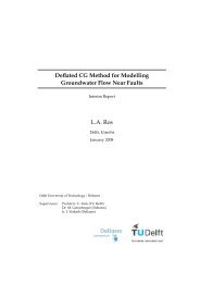
Extension of stochastic volatility equity models 990.060.055Cliquet prices from SZHW and HHW with r x,r= −0.7 and the HestonSchöbel−Zhu−Hull−WhiteHeston−Hull−WhiteHeston0.060.055Cliquet prices from SZHW and HHW with r x,r= 0.7 and the HestonSchöbel−Zhu−Hull−WhiteHeston−Hull−WhiteHeston0.050.05Value of Cliquet at t=00.0450.040.0350.03Value of Cliquet at t=00.0450.040.0350.030.0250.0250.020.020.015−0.1 −0.08 −0.06 −0.04 −0.02 0 0.02 0.040.015−0.1 −0.08 −0.06 −0.04 −0.02 0 0.02 0.04MinCouponMinCouponDownloaded by [Lech A. Grzelak] at 10:55 24 January 2012Figure 1. Pricing a cliquet product under the SZHW, the HHW and the Heston models. Both figures present the price of a globallyfloored cliquet as a function of MinCoupon given by (52) for T ¼ 3 years and M ¼ 36. The remaining parameters are as in table 4.Left: Pricing with x,r ¼ 0.7. Right: Pricing with x,r ¼ 0.7.Value of Diversification product at t = 01.31.251.21.151.11.051Diversification product prices from SZHW and HHW with r x,r= −0.7 and the HestonSchöbel−Zhu−Hull−WhiteHeston−Hull−WhiteHeston0.950 50% 100% 150% 200% 250%ωValue of Diversification product at t = 01.31.251.21.151.11.05Diversification product prices from SZHW and HHW with r x,r= 0.7 and the Heston1Schöbel−Zhu−Hull−WhiteHeston−Hull−WhiteHeston0.950 50% 100% 150% 200% 250%ωFigure 2. Pricing of a diversification hybrid product under different models. The simulations were performed with ¼ 10. Theremaining parameters are as in table 4. Left: Pricing with x,r ¼ 0.7. Right: Pricing with x,r ¼ 0.7.shows that the Heston model generates a significantlyhigher price, whereas the HHW and SZHW prices arerelatively close. The absolute difference between themodels increases with percentage !.4.4. Strategic investment hybrid (best-of-strategy)Suppose that an investor believes that if the price of anasset, S 1 t , goes up, then the equity markets under-performrelative to the interest rate yields, whereas if S 1 t goesdown, the equity markets over-perform relative to theinterest rate (Hunter and Picot 2005/2006). If the prices ofS 1 t are high, the market may expect an increase in inflationand hence in interest rates and low S 1 t prices could havethe opposite effect. In order to include such a feature in ahybrid product we define a contract in which an investoris allowed to buy a weighted performance coupondepending on the performance of another underlying.Such a product can be defined as follows:withðt 0 ¼ 0, T Þ¼E Q ðeV T ¼ max 0, ! L 0þð1L TR T0 r sds V T jF 0 Þ, ð56Þ!Þ S TS 0þ max 0, ð1 !Þ L 0L Tþ ! S TS 01 S 1T >S 1 01 S 1T 5S 1 0,where ! 0 is a weighting factor related to a percentage,and L T ¼ P Mi¼1 PðT, t iÞ with t 1 ¼ T is the T-value of theprojected liabilities for certain time t M , with!4100% !.Figure 3 shows the prices obtained from Monte Carlosimulation of the contract at time t 0 ¼ 0 for maturityT ¼ t 1 ¼ 3 and time horizon t M ¼ 12 with one year spacing.

100 L. A. Grzelak et al.10.9Strategic Investment SZHW, HHW with r x,r= −0.7 and the Heston modelSchöbel−Zhu−Hull−WhiteHeston−Hull−WhiteHeston10.9Strategic Investment SZHW, HHW with r = 0.7 and the Heston modelx,rSchöbel−Zhu−Hull−WhiteHeston−Hull−WhiteHestonValue of Strategic Investment at t = 00.80.70.60.5Value of Strategic Investment at t = 00.80.70.60.50.40.40% 50% 100% 150% 200% 250%ω0% 50% 100% 150% 200% 250%ωFigure 3. Discounted payoffs of the strategic investment hybrid priced with the SZHW, the HHW and the Heston models as afunction of !. The remaining parameters are as in table 4. Left: Pricing with x,r ¼ 0.7. Right: Pricing with x,r ¼ 0.7.Downloaded by [Lech A. Grzelak] at 10:55 24 January 2012Since we did not model the second underlying process, S 1 T ,we assume that S 1 T > S1 0 . We see that, for ! 2 [0%, 100%],the max over the sum of performances disappears andthe hybrid can be relatively easily priced, i.e. separatelyfor both underlyings (L 0 /L T and S T /S 0 ). The differencebetween the stochastic models becomes more pronouncedfor !40% since, then, the correlation plays a moreimportant role. The simulations performed for x,r ¼ 70% and x,r ¼ 70% show that the absolutedifference between the SZHW and HHW models becomessignificant for !4200%. The figure shows that, for small!, the prices of the SZHW and HHW models arerelatively close, whereas the Heston model gives lowerprices for !450%.5. ConclusionsIn this paper we have presented an extension of theScho¨bel–Zhu stochastic volatility model with a Hull–White interest rate process and evaluated it by means ofpricing structured hybrid derivative products.The aim was to define a hybrid stochastic process thatbelongs to the class of affine jump-diffusion models, asthis may lead to efficient calibration of the model. Wehave shown that the so-called Scho¨bel–Zhu–Hull–Whitemodel belongs to the category of affine jump-diffusionprocesses. No restrictions regarding the choice ofcorrelation structure between the different Wiener processesappearing need to be made.We also compared the model with the Heston–Hull–White hybrid model with an indirectly implied correlationbetween the equity and the interest rate. We found thatalthough the model is very attractive because of its squareroot volatility structure, it is unable to generate extremecorrelations.Due to the resulting semi-closed (for Scho¨bel–Zhu–Hull–White) and closed (Heston–Hull–White)characteristic functions we were able to calibrate themodels in an efficient way by means of the Fourier-cosineexpansion pricing technique, adapted to a stochasticinterest rate.It has been shown by numerical experiments fordifferent hybrid products that under the same plainvanilla prices the extended stochastic volatility modelsgive different prices than the Heston model.The present hybrid model cannot model a skew in theinterest rates, which will form part of our future work.AcknowledgementsThe authors would like to thank two anonymous refereesfor valuable suggestions that have significantly improvedthe paper. Moreover, the authors thank NataliaBorovykh and Roger Lord from RabobankInternational and Bin Chen and Fang Fang from theDelft University of Technology for helpful comments.ReferencesAlbanese, C. and Lawi, S., Laplace transforms for integrals ofMarkow processes. Working Paper, 2007. Available onlineat: http://arxiv.org/PS_cache/arxiv/pdf/0710/0710.1599v1.pdf(accessed 2008).Andersen, L.B.G., Efficient simulation of the Heston stochasticvolatility model. J. Comput. Finance, 2007, 11, 1–42.Arnold, L., Stochastic Differential Equations, Theory andApplications, 1973 (Wiley: New York).Brigo, D. and Mercurio, F., Interest Rate Models—Theory andPractice: With Smile, Inflation and Credit, 2nd ed., 2007(Springer: Berlin).Broadie, M. and Kaya, O¨ ., Exact simulation of stochasticvolatility and other affine jump diffusion processes. Oper.Res., 2006, 54, 217–231.Carr, P.P. and Madan, D.B., Option valuation using the fastFourier transform. J. Comput. Finance, 1999, 2, 61–73.

Extension of stochastic volatility equity models 101Downloaded by [Lech A. Grzelak] at 10:55 24 January 2012Cheng, P. and Scaillet, O., Linear–quadratic jump-diffusionmodelling. Math. Finance, 2007, 17, 575–598.Cox, J.C., Ingersoll, J.E. and Ross, S.A., A theory of theterm structure of interest rates. Econometrica, 1985, 53,385–407.Duffie, D., Pan, J. and Singleton, K., Transform analysis andasset pricing for affine jump-diffusions. Econometrica, 2000,68, 1343–1376.Fang, F. and Oosterlee, C.W., A novel pricing method forEuropean options based on Fourier-cosine series expansions.SIAM J. Sci. Comput., 2008a, 31, 826–848.Fang, F. and Oosterlee, C.W., Pricing early-exercise and discretebarrier options by Fourier-cosine series expansions. Workingpaper, 2008b. Available online at: http://ta.twi.tudelft.nl/mf/users/oosterle/oosterlee/bermCOS.pdf (accessed 2008).Fouque, J.P., Papanicolaou, G. and Sircar, K.R., Derivatives inFinancial Markets with Stochastic Volatility, 2000 (CambridgeUniversity Press: Cambridge).Gaspar, R., General quadratic term structures of bond,futures and forward prices. Working Paper Series inEconomics and Finance, 559, Stockholm School ofEconomics, Sweden, 2004.Gatheral, J., The Volatility Surface. A Practitioner’s Guide, 2006(Wiley: New York).Giese, A., On the pricing of auto-callable equity securities in thepresence of stochastic volatility and stochastic interest rates,in Frankfurt, MathFinance Workshop, 2006. Available onlineat: http://www.mathfinance.com/workshop/2006/papers/giese/slides.pdf (accessed 2007).Haastrecht, A., Lord, R., Pelsser, A. and Schrager, D., Pricinglong-maturity equity and FX derivatives with stochasticinterest and stochastic volatility. SSRN Working Paper,2008. Available online at: http://papers.ssrn.com/sol3/papers.cfm?abstract_id=1125590 (accessed 2008).Heston, S., A closed-form solution for options with stochasticvolatility with applications to bond and currency options.Rev. Financial Stud., 1993, 6, 327–343.Hull, J. and White, A., Pricing interest-rate derivative securities.Rev. Financial Stud., 1990, 3, 573–592.Hull, J. and White, A., Using Hull–White interest rate trees.J. Deriv., 1996, 4, 26–36.Hunter, C. and Picot, G., Hybrid derivatives—Financial enginesof the future, in The Euromoney—Derivatives and RiskManagement Handbook, 2005/2006 (BNP Paribas).Lee, R., The moment formula for implied volatility at extremestrikes. Math. Finance, 2004, 14, 469–480.Lewis, A., A simple option formula for general jump-diffusionand other exponential Le´vy processes. SSRN Working Paper,2001. Available online at: http://ssrn.com/abstract=282110(accessed 2007).Lord, R., Private communication, 2007.Lord, R. and Kahl, C., Why the rotation count algorithmworks. Tinbergen Institute Discussion Paper No. 2006-065/2,2006. Available online at: http://ssrn.com/abstract=921335(accessed 2007).Lord, R., Koekkoek, R. and Dijk, D.A comparison ofbiased simulation schemes for stochastic volatility models.Working Paper, Erasmus University Rotterdam, 2007.Available online at: http://www.tinbergen.nl/discussionpapers/06046.pdf (accessed 2007).Mayrhofer, K. and Fischer, F.D., Analytical solutions and anumerical algorithm for the Gauss’s hypergeometric function2F 1 (a, b; c; z). Z. Angew. Math. Mech. (ZAMM), 1996, 74,265–273.Muskulus, M., in’t Hout, K., Bierkens, J., van der Ploeg, A.P.C.,in’t Panhuis, J., Fang, F., Janssens, B. and Oosterlee, C.W., TheING problem—Aproblem fromfinancial industry; threepaperson the Heston–Hull–White model. in Proceeding ofMathematics with Industry, 2007, pp. 91–115.Oksendal, B., Stochastic Differential Equations; An Introductionwith Applications, 3rd ed., 1992 (Springer: New York).Scho¨bel, R. and Zhu, J., Stochasic volatility with an Ornstein–Uhlenbeck process: an extension. Eur. Financial Rev., 1999, 3,23–46.Schurz, H., Asymptotical mean square stability of an equilibriumpoint of some linear numerical solutions with multiplicativenoise. Stoch. Anal. App., 1996, 14, 313–353.Shreve, S.E., Stochastic Calculus Models for Finance: ContinuousTime Models, 2004 (Springer: New York).Stein, J.C. and Stein, E.M., Stock price distributions withstochastic volatility: an analytic approach. Rev. FinancialStud., 1991, 4, 727–752.Vasˇiček, O.A., An equilibrium characterization of the termstructure. J. Financial Econ., 1977, 5, 177–188.Wilmott, P., Cliquet options and volatility models. WILMOTTMag., 2002, Dec, 78–83.Appendix A: Proofs of various lemmasIn this appendix we report the proofs of the variouslemmas.A.1. Proof of lemma 2.3Proof:We need to find the solution ofdd Aðu, Þ ¼ r 0 þ B T a 0 þ 1 2 BT c 0 B, ðA1Þdd Bðu, Þ ¼ r 1 þ a T 1 B þ 1 2 BT c 1 B: ðA2ÞFor the space vector X t ¼½ex t,er t , v t , t Š T we have2130 120a 0 ¼½0, 0, 2 , Š T 0 0 0, a 1 ¼ 674 0 0 2 2 5 ,0 0 0 2 301r 0 ¼ 0, r 1 ¼ 6 74 0 5 ,0and:¼ ðX t ÞðX t Þ T ¼This leads to230 0 0 0 20 r,c 0 ¼64 0 075 , 2264v x,r 2v x,v x, 2 2 r,v r,4v 2 2 2 2375 :23ð0,0,1,0Þ ð0,0,0, x,r Þ ð0,0,2 x,v ;0Þ ð0,0,0, x, Þð0,0,0,0Þ ð0,0,0,2 r,v Þ ð0,0,0,0Þc 1 ¼64ð0,0,4 2 ,0Þ ð0,0,0,2 2 Þ75 :ð0,0,0,0Þ

102 L. A. Grzelak et al.Downloaded by [Lech A. Grzelak] at 10:55 24 January 2012With2 P 4 P 4i¼1 j¼1 B 3i½s 1 ð1ÞŠ i, j B j12 BT c 1 B ¼ 1 P 4 P 4i¼1 j¼1 B i½s 1 ð2ÞŠ i, j B jP2 4 P 4i¼1 j¼1 B 6i½s 1 ð3ÞŠ i, j B j745P 4 P 4i¼1 j¼1 B i½s 1 ð4ÞŠ i, j B j(with i ¼ 1, ..., 4 representing x, v, r, ) we obtain thefollowing system:2 30dAd ¼½B 0x, B r , B v , B Š64 2 7523230 0 0 0 B xþ 1 2 ½B 2 0 r,B rx, B r , B v , B Š67674 0 0 545 ,2dB x3 2 3d 0dBdBrd ¼d6 dB4v 7d 5 ¼ 16 74 0 5dB 0d2320 0 0 01 0 0þ 6176420 2 0 540 0 2 whereB xB rB vB 2S 1 ¼ B 2 x þ 4 x,vB x B v þ 4 2 B 2 v ,B vB ðA3Þ3 2 3075 þ 1 06 72 4 S 1 5 ,S 2ðA4ÞðA5ÞS 2 ¼ 2 x,r B x B r þ 2 x, B x B þ 4 r,v B r B v þ 4 2 B v B :ðA6ÞSimplification of equations (A3) and (A4) finishes theproof.œA.2. Proof of lemma 2.4Proof: In the 1D case, i.e. u ¼ [u,0,0,0] T , we start bysolving the ODE for dB r ,dd B r þ B r ¼ iu 1:Standard calculations giveZ 0dðe s B r ðu, sÞÞ ¼ ðiu1ÞZ 0e s ds,i.e. e B r ðu, Þ e 0 1 1B r ðu,0Þ¼ðiu 1Þ e :Using the boundary condition B r (u, 0)¼ 0 gives B r (u, ) ¼(1/)(iu 1)(1 e t ).The ODE for B v now reads (using B x ¼ iu)dd B v ¼ 1 2 uði þ uÞþ2 2 Bv 2 2ð x,v iuÞB v : ðA7ÞIn order to simplify this equation we introduce thevariables ¼ 1 2 uði þ uÞ and ¼ 2( x,viu). The ODEcan then be presented in the following form:dd B v ¼ B v þ 2 2 Bv 2 : ðA8ÞFollowing the calculations for the Heston model thesolution of (A8) readsB v ðu, Þ ¼ d 1 e d 4 2 1 e d ,ðb=aÞpwhere ffiffiffiffiffiffiffiffiffiffiffiffiffiffiffiffiffiffiffiffiffi a ¼ þ d/4 2 , b ¼ ( d )/(4 2 ) and d ¼ 2 8 2 . This solution can be simplified to1 e d B v ðu, Þ ¼b1 g e d ,with g ¼ ( d )/( þ d ).Next, we solve the ODE for B ,dd B ¼ð2B v þ x,r B x B r þ 2 r,v B r B v Þþð x, B x þ 2 2 B v ÞB : ðA9ÞWe introduce the following functions:ðÞ ¼2B v þ x,r B x B r þ 2 r,v B r B v , ðA10ÞðÞ ¼ x, B x þ 2 2 B v : ðA11ÞThis leads to the following ODE:dd B ðÞB ¼ ðÞ,whose solution follows fromRd d ðe ðsÞds 0 B Þ¼ðÞ expor Z Z exp ðsÞds B ¼ ðsÞ exp0So, finally, we need to calculateZ Z B ðu, Þ ¼exp ðsÞds ðsÞ expB ðu,0Þ¼0:000Z 0ðsÞds ,Z s0Z s0ðkÞdk ds:ðkÞdk ds,ðA12Þ

Extension of stochastic volatility equity models 103Downloaded by [Lech A. Grzelak] at 10:55 24 January 2012For this, we start with the integral for (k),Z sZ sðkÞdk ¼ ð x, iu þ 2 2 B v Þdk00¼ x, iu þ d s2g ð d Þðg 1Þþ log esd g2dg 1 g ¼ C 1 s þ C 2 log esd g, ðA13Þ1 gwhere C 1 ¼ { x, iu þ [( pd )/2g]}, C 2 ¼ [( d )( g 1)]/2dg, ¼ 2( x,v iu), d ¼ ffiffiffiffiffiffiffiffiffiffiffiffiffiffiffiffiffiffiffiffiffi 2 8 2 and g ¼ ( d )/( þ d ). After substitution of these quantities, we find thatC 1 ¼ D/2 and C 2 ¼ 1.Next, we need to calculate the exponent of the integralof ,Z s exp ðkÞdk ¼ exp C 1 s þ C 2 log esd g01 g¼ exp sd 1 g2 e sd , ðA14Þgand we can include in the integral,Z Z sðsÞ exp ðkÞdk ds0Z 0Z 0¼ ð2B v þ x,r B x B r þ 2 r,v B r B v Þ0 d esd exp2 s gds:ðA15Þ1 gThis integral is split into three parts. The first part can besolved analytically,Z 2B v e ðd=2Þs e sd gds01 gZ 1 e sd ¼ 2b1 e sd e ðd=2Þs e sd gdsg 1 g¼ 2b1 g0e sd=2 e sd¼ 16b sinh 2 ðd=4Þð1 gÞd1 ds f 11 g : ðA16ÞThe second part can also be solved analytically,Z x,r B x B r e ðd=2Þs e sd gds01 gZ 1¼ x,r0 iuðiu 1Þð1 e s Þe sd=2 e sd gds1 g¼ Zx,riuðiu 1Þ e sd=2 ð1 e s Þðe sd gÞdsð1 gÞ 0¼ x,riuðiu 1Þð f 2 f 3 Þ, ðA17Þð1 gÞwheref 2 ¼ 2 d ðed=21Þþ 2gd ðe d=2 1Þ ðA18Þf 3 ¼ 2ðeð=2Þðd 2Þ 1Þ 2gð1 e ð=2Þðdþ2Þ Þ, ðA19Þd 2d þ 2and the third part readsZ 2 r,v B r B v e ðd=2Þs e sd gds01 g¼ 2 Z r,vB r B v e ðd=2Þs ðe sd gÞds1 g 0¼ 2 Zr,vðiu 1Þb e ð1=2Þsðdþ2Þ ðe sd 1Þðe s 1Þdsð1 gÞ 0¼ 2 r,vðiu 1Þbð f 4 þ f 5 Þ,ðA20Þð1 gÞwheref 4 ¼ 2d 24d þ 2d þ 2 ,f 5 ¼ðe ð1=2Þðdþ2Þ Þ 2e ð1 þ e d ÞdSo, finally, we haveZ Z B ðu, Þ ¼exp ðsÞds ðsÞ exp002e dd 2Z s0ðA21Þ2:d þ 2ðA22ÞðkÞdk ds¼ f 0 f 1 þ 1 x,riuðiu 1Þð f 2 f 3 Þþ 1 2 r,vbðiu 1Þð f 4 þ f 5 ÞÞ, ðA23Þwith f 0 ¼ e (d/2) /(e d g), f 2 and f 3 from (A18) and (A19),respectively, f 4 from (A21) and f 5 from (A22).Now we solve the ODE for A(u, ),dd A ¼ 2 B v þ B þ 1 2 2 B 2 r þ 1 2 2 B 2 þ r,B B r ,with solutionZ ðA24ÞZ Aðu,Þ Aðu,0Þ¼ 2 B v ds þ B ds þ 1 Z 00 2 2 Br 2 ds0þ 1 Z Z 2 2 B 2 ds þ r, B B r ds,00ðA25ÞorZ Aðu, Þ ¼ 2 B v þ 1 0 2 2 Br2 ds|fflfflfflfflfflfflfflfflfflfflfflfflfflfflfflfflfflfflffl{zfflfflfflfflfflfflfflfflfflfflfflfflfflfflfflfflfflfflffl}A 1 ðu, ÞZ þ B þ 1 0 2 2 B þ r, B r ds : ðA26Þ|fflfflfflfflfflfflfflfflfflfflfflfflfflfflfflfflfflfflfflfflfflfflfflfflfflfflfflfflfflfflffl{zfflfflfflfflfflfflfflfflfflfflfflfflfflfflfflfflfflfflfflfflfflfflfflfflfflfflfflfflfflfflffl}ðu, Þ

104 L. A. Grzelak et al.Downloaded by [Lech A. Grzelak] at 10:55 24 January 2012In order to find A(u, ) we have to evaluate the integralsA 1 (u, ) and (u, ). Integral (u, ) involves a hypergeometricfunction (called the 2 F 1 function or simply theGaussian function), which is computed numerically here.For integral A 1 (u, ) we have two representations,orA 1 ðu, Þ ¼whereA 1 ðu, Þ ¼12 2 log g e sd 1g 11 esd glog221 gþ f 612 3 f 7,þ f 612 3 f 7,ðA27ÞðA28Þf 6 ¼ 1 ð d Þ, ðA29Þ42f 7 ¼ðiu 1Þ 2 ð3 þ e 2 4e 2Þ: ðA30ÞSince a complex-valued logarithm appears in A 1 (u, ), itshould be treated with some care. It turns out that thesecond formulation gives rise to discontinuities that maycause inaccuracies. According to Lord and Kahl (2006),an easy way to avoid any errors due to complex-valueddiscontinuities is to apply numerical integration.We know that the price of a zero coupon bondcan be obtained from the characteristic function SZHW (u, X t , t, T ) by setting u ¼ [0, 0, 0, 0] T . Therefore,Pðt,TÞ¼ð0,X t ,Þ¼ expZ Ttþ B v ð0,Þv t þ B ð0,Þ t Þ:Since er 0 ¼ 0, we havePð0, T Þ¼exps ds expðAð0,ÞþB x ð0,Þx t þ B r ð0,Þer tZ T0ðA31Þs ds expðAð0, ÞþB x ð0, Þx 0þ B v ð0, Þv 0 þ B ð0, Þ 0 Þ,and it is easy to check that B x (0, T ) ¼ 0, B v (0, T ) ¼ 0,B (0, T ) ¼ 0 andAð0, T Þ¼ 1 Z T2 2 B r ð0, sÞ 2 ds0¼ 2 3 12 3 2 2 e 2T þ 2e T þ T : ðA32ÞR TTherefore, Pð0, T Þ¼expð0 s ds þ Að0, T ÞÞ orlog ðPð0, T ÞÞ ¼R T0 s ds þ Að0, T Þ, which finally givesT ¼@@T logPð0,TÞþ @2Að0,TÞ¼fð0,TÞþ@T 2 ð1 e T Þ 2 ,2ðA33Þsince 0 ¼ f(0, 0) r 0 , where r 0 is the initial value of theinterest rate process r t . With u ¼ [u, 0,0,0] T , we find SZHW ðu, X t , t, T Þ¼expðeAðu, ÞþB x ðu, Þx t þ B r ðu, Þ~r tþ B v ðu, Þv t þ B ðu, Þ t Þ, ðA34ÞwitheAðu, Þ¼¼ðiu¼ð1Z TtZ Tt1ÞiuÞð1Z Ts ds þ iuZ TtZ Tts ds þ Aðu, Þtf ð0, sÞþ 2 2 ð1 e s Þ 2 ds þ Aðu, Þ2dðlogðPð0, sÞÞÞ þ ð1 iuÞ 2e s Þ 2 ds þ Aðu, Þ2 2¼ð1 iuÞ log Pð0, T Þ þð1 iuÞ 2Pð0, tÞ2 2 ðT tÞþ 2 ðe T e t 1 2TÞ ðe e2þ Aðu, Þ,2t ÞðA35Þand A(u, ) as in (A26). Now, by setting (x) ¼ exp(x/2)the discounted CF for the Scho¨bel–Zhu–Hull–White hybrid process is determined and the proof isfinished.œA.3. Proof of lemma 2.4Proof: As in the case of the SZHW hybrid model weneed to find the solution ofdd Aðu, Þ ¼ r 0 þ B T a 0 þ 1 2 BT c 0 B, ðA36Þdd Bðu, Þ ¼ r 1 þ a T 1 B þ 1 2 BT c 1 B: ðA37ÞFor the space vector X t ¼½ex t,er t , t Š T we haveanda 0 ¼r 0 ¼ 0, 1T2 S,r 2 ,0, , a 1 ¼2 306 7r 1 ¼ 4 1 5,0:¼ ðX t ÞðX t Þ T ¼2310 12674 0 0 5,0 0 23 t þ S,r 2 S,r x, t4 2 0 5: 2 tThis leads to23S,r 2 S,r 0c 0 ¼ 6 S,r 2 0 745 ,0 0 02ð0, 0, 1Þ ð0, 0, 0Þ3ð0, 0, x, Þ6c 1 ¼ 4 ð0, 0, 0Þ ð0, 0, 0Þ ð0, 0, 0Þ75:ð0, 0, x, Þ ð0, 0, 0Þ ð0, 0, 2 Þ

Downloaded by [Lech A. Grzelak] at 10:55 24 January 2012Extension of stochastic volatility equity models 105With2 P 3 P 412 BT c 1 B ¼ 1 i¼1 j¼1 B 3i½s 1 ð1ÞŠ i, j B j6 P 3 P 4i¼1 j¼12B 74i½s 1 ð2ÞŠ i, j B j 5P 3 P 4i¼1 j¼1 B i½s 1 ð3ÞŠ i, j B j(with i ¼ 1, ..., 3 representing x, r, ) we obtain thefollowing system:212dA 3S,r2d ¼½B 6 7x, B r , B Š40 5 þ 1 2 ½B x, B r , B Š 2323S,r 2 S,r 0 B x6 4 S,r 2 7670 54B r 5, ðA38Þ0 0 0 B 2 3dB x2 3ddBd ¼6 dB r 74 d 5 ¼ 6 7401 5dB 0d2320 0 06þ 1 076454120 whereB xB rB S 1 ¼ B 2 x þ 2 xB x B þ 2 B 2 :3 2 375 þ 1 06 74 0 5, ðA39Þ2S 1ðA40ÞNow, simplification of equations (A38) and (A39) finishesthe proof.œ