Addendum to the Restoration Plan for the Northwest Fork of the ...
Addendum to the Restoration Plan for the Northwest Fork of the ...
Addendum to the Restoration Plan for the Northwest Fork of the ...

You also want an ePaper? Increase the reach of your titles
YUMPU automatically turns print PDFs into web optimized ePapers that Google loves.
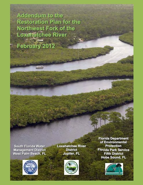
<strong>Addendum</strong> <strong>to</strong> <strong>the</strong>Res<strong>to</strong>ration <strong>Plan</strong> <strong>for</strong> <strong>the</strong><strong>Northwest</strong> <strong>Fork</strong> <strong>of</strong> <strong>the</strong>Loxahatchee RiverFebruary 2012Soutth Fllorriida WatterrManagementt DiisttrriicttWestt Pallm Beach,, FLLoxahattchee RiiverrDiisttrriicttJupiitterr,, FLFllorriida Deparrttment<strong>to</strong>ff EnviirronmenttallPrrottecttiionFllorrriida Parrk SerrviiceFiifftth DiisttrriicttHobe Sound,, FL
This page is intentionally left blank.
Executive SummaryEXECUTIVE SUMMARYOften referred <strong>to</strong> as <strong>the</strong> last free flowing river in South Florida, <strong>the</strong> <strong>Northwest</strong> <strong>Fork</strong> <strong>of</strong> <strong>the</strong>Loxahatchee River is one <strong>of</strong> only two federally-designated Wild and Scenic Rivers in Florida.The Wild and Scenic portion <strong>of</strong> this river consists <strong>of</strong> 9.5 miles <strong>of</strong> freshwater riverine and tidalfloodplain that provides essential habitat. A combination <strong>of</strong> <strong>the</strong> opening <strong>of</strong> Jupiter Inlet, sea levelrise, diversion <strong>of</strong> flows from <strong>the</strong> <strong>Northwest</strong> <strong>Fork</strong> <strong>to</strong> <strong>the</strong> Southwest <strong>Fork</strong>, and development hasresulted in significant encroachment <strong>of</strong> saltwater and saltwater <strong>to</strong>lerant mangroves in<strong>to</strong> what wasonce a large expanse <strong>of</strong> bald cypress freshwater floodplain.To begin <strong>to</strong> address <strong>the</strong>se issues, <strong>the</strong> South Florida Water Management District (SFWMD)developed and adopted a Minimum Flows and Levels (MFL) Rule in 2003 (Chapter 40E, FloridaAdministrative Code). The MFL criteria were written <strong>to</strong> protect <strong>the</strong> remaining floodplain swampcommunity from “significant harm”:A MFL violation occurs within <strong>the</strong> <strong>Northwest</strong> <strong>Fork</strong> <strong>of</strong> <strong>the</strong> Loxahatchee River when anexceedance <strong>of</strong> <strong>the</strong> minimum flow criteria occurs more than once every six years. An“exceedance” is defined as when Lainhart Dam flows <strong>to</strong> <strong>the</strong> <strong>Northwest</strong> <strong>Fork</strong> <strong>of</strong> <strong>the</strong> riverdecline below 35 cubic feet per second (cfs) <strong>for</strong> more than 20 consecutive days withinany given calendar year or when <strong>the</strong> 20-day moving average salinity measured at RiverMile 9.2 exceeds 2 psu [practical salinity units].As required by <strong>the</strong> MFL legislation, a recovery strategy was developed. This strategy committed<strong>the</strong> SFWMD and <strong>the</strong> Florida Department <strong>of</strong> Environmental Protection (FDEP) <strong>to</strong> develop “apractical res<strong>to</strong>ration plan and goal” (SFWMD 2002a).Staff from <strong>the</strong> SFWMD, FDEP Florida Park Service (FPS) District 5, and Loxahatchee RiverDistrict (LRD) collected and analyzed data and developed <strong>to</strong>ols and models <strong>to</strong> investigate effects<strong>of</strong> several res<strong>to</strong>ration flow scenarios on <strong>Northwest</strong> <strong>Fork</strong> flora and fauna. Although emphasis wasplaced on improving conditions in <strong>the</strong> floodplain and along riverine portions <strong>of</strong> <strong>the</strong> <strong>Northwest</strong><strong>Fork</strong>, downstream ecological indica<strong>to</strong>rs were evaluated under increased flow scenarios <strong>to</strong> assure<strong>the</strong>se flows would not detrimentally affect <strong>the</strong> Loxahatchee Estuary. A “preferred res<strong>to</strong>rationflow scenario” that incorporated both dry and wet season hydrologic flow patterns wasdetermined. This scenario is expected <strong>to</strong> provide <strong>the</strong> greatest ecological benefit <strong>to</strong> <strong>the</strong> freshwaterriverine and tidal floodplain with minimal impact on <strong>the</strong> estuary. The preferred res<strong>to</strong>ration flowscenario includes a variable dry season flow between 50 and 110 cfs, with a 69 cfs mean monthlyflow over Lainhart Dam, while providing an additional 30 cfs <strong>of</strong> flow from downstreamtributaries. These ef<strong>for</strong>ts are documented in <strong>the</strong> Res<strong>to</strong>ration <strong>Plan</strong> <strong>for</strong> <strong>the</strong> <strong>Northwest</strong> <strong>Fork</strong> <strong>of</strong> <strong>the</strong>Loxahatchee River (SFWMD 2006) available at www.sfwmd.gov.In addition <strong>to</strong> <strong>the</strong> preferred res<strong>to</strong>ration flow scenario, <strong>the</strong> res<strong>to</strong>ration plan recommended(1) development <strong>of</strong> a science plan <strong>for</strong> <strong>the</strong> Loxahatchee River and (2) a five-year update <strong>of</strong> <strong>the</strong>res<strong>to</strong>ration plan. The purpose <strong>of</strong> <strong>the</strong> science plan was <strong>to</strong> 1) moni<strong>to</strong>r effects <strong>of</strong> res<strong>to</strong>ration ef<strong>for</strong>ts<strong>to</strong> support adaptive management <strong>of</strong> <strong>the</strong> system and 2) fill knowledge gaps critical <strong>to</strong> ecosystemres<strong>to</strong>ration success. The Loxahatchee River Science <strong>Plan</strong> (SFWMD et al. 2010) was completedin 2010 and is also available at www.sfwmd.gov.iii
Executive SummarySince 2006, moni<strong>to</strong>ring ef<strong>for</strong>ts recommended by <strong>the</strong> res<strong>to</strong>ration plan have been conducted. Theseef<strong>for</strong>ts culminated in this <strong>Addendum</strong> <strong>to</strong> <strong>the</strong> Res<strong>to</strong>ration <strong>Plan</strong> <strong>for</strong> <strong>the</strong> <strong>Northwest</strong> <strong>Fork</strong> <strong>of</strong> <strong>the</strong>Loxahatchee River. This addendum is a compilation <strong>of</strong> new knowledge gained during <strong>the</strong> lastfive years and focuses on analysis <strong>of</strong> fac<strong>to</strong>rs identified in <strong>the</strong> 2006 res<strong>to</strong>ration plan as needingmore attention. The new research and moni<strong>to</strong>ring results were organized in<strong>to</strong> six majorcategories: (1) salinity and stage, (2) floodplain vegetation, (3) floodplain fish and wildlife,(4) estuarine flora and fauna, (5) water quality, and (6) res<strong>to</strong>ration progress. In addition, thisaddendum evaluates <strong>the</strong> 2006 flow scenario in light <strong>of</strong> <strong>the</strong> results <strong>of</strong> <strong>the</strong>se moni<strong>to</strong>ring ef<strong>for</strong>ts.Generally, <strong>the</strong> new in<strong>for</strong>mation fur<strong>the</strong>r validates <strong>the</strong> recommendations made in <strong>the</strong> 2006res<strong>to</strong>ration plan.Salinity and stage are discussed in Section 2.0. The freshwater flow–salinity relationships atRiver Mile (RM) 9.1 and Kitching Creek were revisited confirming <strong>the</strong> relationships establishedin <strong>the</strong> res<strong>to</strong>ration plan and showing a 99.9 percent probability that salinity at RM 9.1 will remainbelow 2 psu provided freshwater flow over Lainhart Dam remains above 35 cfs. The flow–stagerelationships established in <strong>the</strong> res<strong>to</strong>ration plan <strong>for</strong> at RM 11 and RM 12 were also re-evaluatedand confirmed.The estimated average groundwater seepage upstream <strong>of</strong> RM 6 was found <strong>to</strong> be around 9 cfswith a minimum <strong>of</strong> 2 cfs and a maximum <strong>of</strong> 14 cfs. Compared with <strong>the</strong> minimum flow target <strong>of</strong>35 cfs, <strong>the</strong> groundwater contribution <strong>to</strong> <strong>the</strong> river can be a significant source <strong>of</strong> fresh water,particularly in <strong>the</strong> dry season. The implication is that wetland res<strong>to</strong>ration in <strong>the</strong> watershed willhelp achieve a healthy groundwater contribution <strong>to</strong> <strong>the</strong> river.In order <strong>to</strong> evaluate <strong>the</strong> potential impact <strong>of</strong> sea level rise on <strong>the</strong> stage <strong>of</strong> <strong>the</strong> <strong>Northwest</strong> <strong>Fork</strong> tidalfloodplain stage, an analytical solution was derived based on a tidal-averaged one-dimensionalmodel. The derived analytical solution suggests <strong>the</strong> influence <strong>of</strong> downstream tidal stage could begreater on floodplain stage than watershed inflow.Floodplain soil moisture, ground water stage and Lainhart Dam flow relationships weredeveloped <strong>to</strong> help manage flows and stages <strong>for</strong> a healthier floodplain community. It was foundthat infiltration <strong>of</strong> salt water inundated on <strong>the</strong> floodplain during high tides, not <strong>the</strong> diffusion <strong>of</strong>salt water in <strong>the</strong> river <strong>to</strong> <strong>the</strong> aquifer, contributed <strong>to</strong> high porewater salinity in <strong>the</strong> floodplain. Thisfinding suggests tidal inundation <strong>of</strong> <strong>the</strong> floodplain should be <strong>the</strong> emphasis <strong>for</strong> salinity control in<strong>the</strong> floodplain.Section 3.0 presents results from vegetation surveys. Five additional tree species (blackmangrove, cocoplum, mulberry, climbing cassia and poison ivy) have been introduced. Increasesin abundance and relative abundance <strong>of</strong> tree species were attributed mainly <strong>to</strong> white mangroveand pond apple, while <strong>the</strong>re were losses in bald cypress, cabbage palm, wax myrtle, Brazilianpepper and red maple. Most <strong>of</strong> <strong>the</strong> losses were attributed <strong>to</strong> damage from <strong>the</strong> 2004–2005hurricanes, saltwater intrusion, and exotic removal programs within Jonathan Dickinson StatePark. The highest percentage <strong>of</strong> shrub coverage was provided by lea<strong>the</strong>r fern, pond apple, swampfern, red mangrove and tri-veined fern. Cabbage palm shrubs were more abundant on riverinetransects and responded negatively <strong>to</strong> <strong>the</strong> 2007 drought and positively <strong>to</strong> increased freshwaterdry season flows in 2010. Few bald cypress shrubs were present. Groundcover was dominated bytri-vein fern, white mangrove, water hyssop and penny wort. White mangrove seedlings showediv
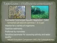
Executive Summarya positive reaction <strong>to</strong> <strong>the</strong> 2007 drought and a negative reaction <strong>to</strong> <strong>the</strong> increased freshwater dryseason flows in 2010. Bald cypress showed an increase in seedling production; however, most <strong>of</strong><strong>the</strong>se seedlings were present on transects <strong>of</strong> <strong>the</strong> upper tidal reach, which characteristically haslower salinity and is tidally inundated twice daily. During <strong>the</strong> vegetative surveys, 30 nonnativespecies were encountered within <strong>the</strong> floodplain. The Loxahatchee River VegetationalDemonstration Research project showed that if exotic vegetation is removed, native vegetationcan naturally recruit back in<strong>to</strong> areas <strong>of</strong> <strong>the</strong> upper tidal reach.Results <strong>of</strong> various wildlife moni<strong>to</strong>ring were analyzed in Section 4.0. The purpose <strong>of</strong> thismoni<strong>to</strong>ring was <strong>to</strong> obtain pre-res<strong>to</strong>ration baseline data. Few frogs with longer life cycles wereobserved, indicating that perhaps water levels were not sufficient in <strong>the</strong> observed years <strong>to</strong>adequately sustain <strong>the</strong>m. This should change with res<strong>to</strong>rative flows and <strong>the</strong> system could bemanaged in <strong>the</strong> future <strong>to</strong> have an excess <strong>of</strong> 90 days <strong>of</strong> inundation in <strong>the</strong> floodplain. Alliga<strong>to</strong>rs areusing <strong>the</strong> freshwater (i.e. ≤ 1 psu) portions <strong>of</strong> <strong>the</strong> river much more than <strong>the</strong> lower tidal reaches <strong>of</strong><strong>the</strong> river perhaps due <strong>to</strong> higher salinity. The riverine reach <strong>of</strong> <strong>the</strong> river supports a wider variety <strong>of</strong>species due <strong>to</strong> <strong>the</strong> older and more complex vegetation community structure. Drying out <strong>of</strong> <strong>the</strong>riverine reach <strong>of</strong> <strong>the</strong> river allows <strong>for</strong> small mammals <strong>to</strong> utilize this part <strong>of</strong> <strong>the</strong> floodplain <strong>for</strong>longer periods <strong>of</strong> time; however it is more important <strong>for</strong> aquatic species <strong>to</strong> have an inundatedfloodplain <strong>for</strong> <strong>the</strong>ir life cycle events. No one species or set <strong>of</strong> species was found <strong>to</strong> be clear cutcandidates <strong>for</strong> potential indica<strong>to</strong>rs <strong>of</strong> river health, but alliga<strong>to</strong>rs and small mammals seem <strong>to</strong> have<strong>the</strong> clearest relationship with fresh water in <strong>the</strong> river and floodplain. The Florida Park Service,who conducted <strong>the</strong>se studies, recommends fur<strong>the</strong>r study <strong>of</strong> <strong>the</strong>se species. It is important that onceres<strong>to</strong>rative flows reach <strong>the</strong> river floodplain, this work be revisited <strong>for</strong> <strong>the</strong> sake <strong>of</strong> comparison.Section 5.0 contains new research and moni<strong>to</strong>ring results <strong>for</strong> seagrass and oysters. Detailedspecies mapping results confirmed that shoal grass and Johnson’s seagrass are <strong>the</strong> dominantseagrass species throughout <strong>the</strong> estuary. Maps from aerial pho<strong>to</strong>graphs revealed <strong>the</strong> dynamicnature <strong>of</strong> <strong>the</strong> core seagrass beds. An apparent increasing trend in seagrass acreage was observed,but only shoal grass and Johnson’s seagrass successfully recruited <strong>to</strong> <strong>the</strong> darker water areas with<strong>the</strong> greatest salinity variations. Seagrass species diversity and coverage increased downstream <strong>of</strong>RM 2 because <strong>of</strong> more stable and higher salinity. The dynamic nature <strong>of</strong> <strong>the</strong> sediments in <strong>the</strong>Loxahatchee River Estuary may play an important role in seagrass distribution includingspecies distribution.The patterns <strong>of</strong> oyster abundance, health, and population ecology within <strong>the</strong> Loxahatcheegenerally fell within <strong>the</strong> bounds expected <strong>for</strong> South Florida oyster populations. Through anAmerican Recovery and Reinvestment Act <strong>of</strong> 2009 stimulus grant, an oyster reef habitatres<strong>to</strong>ration project was initiated on June 21, 2010 by <strong>the</strong> LRD and <strong>the</strong>ir partners. The projectsignificantly increased suitable oyster recruitment substrate from approximately 8.5 <strong>to</strong> 13.5acres. It is expected that overall acreage <strong>of</strong> live oyster reefs in <strong>the</strong> Loxahatchee River Estuarywill ultimately increase with <strong>the</strong> addition <strong>of</strong> this suitable substrate.A significant supplement <strong>of</strong> this addendum <strong>to</strong> <strong>the</strong> res<strong>to</strong>ration plan is <strong>the</strong> water quality status andnutrient loads estimation presented in Section 6.0. Water quality in <strong>the</strong> Loxahatchee River in2010 was generally good. Total nitrogen and <strong>to</strong>tal phosphorus concentrations were generallybelow target values established by <strong>the</strong> United States Environmental Protection Agency and LRD.Elevated chlorophyll a concentrations, particularly in <strong>the</strong> meso/oligohaline and brackish waterv
Executive Summarytributaries, and low dissolved oxygen levels were observed at a variety <strong>of</strong> sampling sitesthroughout <strong>the</strong> watershed. Fur<strong>the</strong>r investigation in<strong>to</strong> <strong>the</strong> causes and potential consequences <strong>of</strong> <strong>the</strong>elevated chlorophyll a concentration is needed.Water quality and flow data were used <strong>to</strong> estimate nutrient loads <strong>to</strong> <strong>the</strong> estuary from 2003 <strong>to</strong>2008. The estimated nutrient loads that flow over Lainhart Dam contributed 65 percent <strong>of</strong> <strong>the</strong>dissolved inorganic nitrogen <strong>to</strong> <strong>the</strong> river while Cypress Creek is <strong>the</strong> major contribu<strong>to</strong>r in <strong>to</strong>talnitrogen (45%), dissolved inorganic phosphorus (47%), and <strong>to</strong>tal phosphorus (52%). Also,increased flows and associated nutrient loads will generally increase nutrient concentrations andreduce oxygen content and water clarity in <strong>the</strong> downstream areas, but no discernable increase inchlorophyll a was observed.Lastly, Section 7.0 describes res<strong>to</strong>ration progress. The Comprehensive Everglades Res<strong>to</strong>ration<strong>Plan</strong>’s Loxahatchee River Watershed Res<strong>to</strong>ration Project (<strong>for</strong>merly <strong>the</strong> North Palm BeachCounty – Part 1 Project) has already completed acquisition <strong>of</strong> <strong>the</strong> L-8 Reservoir, construction <strong>of</strong><strong>the</strong> Control 2 pump station and G-160 and G-161 structures, and widening <strong>of</strong> <strong>the</strong> M-Canal. In <strong>the</strong>dry season from March 1 <strong>to</strong> April 19, 2011, <strong>the</strong> L-8 Reservoir Pilot Test Project was successfullyimplemented. The project was a collaborative ef<strong>for</strong>t between <strong>the</strong> SFWMD, City <strong>of</strong> West PalmBeach, Palm Beach County and LRD. The primary purpose <strong>of</strong> <strong>the</strong> project was <strong>to</strong> provideoperational testing <strong>of</strong> <strong>the</strong> existing facilities’ ability <strong>to</strong> deliver flows <strong>to</strong> <strong>the</strong> <strong>Northwest</strong> <strong>Fork</strong> <strong>of</strong> <strong>the</strong>Loxahatchee River. One conclusion from <strong>the</strong> test was that delivering ‘dedicated water’ from <strong>the</strong>L-8 Reservoir <strong>to</strong> Grassy Waters Preserve and <strong>the</strong> <strong>Northwest</strong> <strong>Fork</strong> <strong>of</strong> <strong>the</strong> Loxahatchee River had amultitude <strong>of</strong> complexities and constraints related <strong>to</strong> operations, water quality, wildlife concerns,public water supply and water losses. Data collected from <strong>the</strong> pilot project will be used <strong>to</strong>provide <strong>the</strong> technical basis <strong>for</strong> validation <strong>of</strong> modeling <strong>to</strong>ols needed <strong>to</strong> design <strong>the</strong> L-8 pumpstation.vi
Table <strong>of</strong> ContentsTABLE OF CONTENTSAcknowledgementsiExecutive SummaryiiiTable <strong>of</strong> ContentsviiList <strong>of</strong> TablesxList <strong>of</strong> FiguresxiiiAcronyms and Units <strong>of</strong> Measurementxxi1.0 Introduction 12.0 Salinity and Stage as System Health Indica<strong>to</strong>rs 52.1 Flow-Salinity Relationship ................................................................................................. 52.2 Groundwater Contribution <strong>to</strong> Flow ................................................................................... 102.3 Tidal Influence .................................................................................................................. 142.3.1 Tidal and Salinity Surge during 2004 Hurricane Season .......................................... 152.3.2 Tidal Stage and Floodplain Inundation ..................................................................... 152.4 Soil Moisture, Groundwater Salinity and Pore Water Salinity ......................................... 222.4.1 Soil Moisture ............................................................................................................. 232.4.2 Groundwater Stage .................................................................................................... 282.4.3 Groundwater Salinity ................................................................................................ 312.4.4 Porewater Salinity ..................................................................................................... 312.4.5 Porewater Salinity Variation in <strong>the</strong> Upper Tidal Floodplain .................................... 342.5 Flow-Stage Relationship ................................................................................................... 593.0 Riverine and Tidal Floodplain Vegetation Indica<strong>to</strong>rs 733.1 Vegetation Surveys ........................................................................................................... 743.1.1 Summary <strong>of</strong> Methods ................................................................................................ 773.1.2 Rainfall and Freshwater Flow ................................................................................... 783.1.3 Canopy Communities ................................................................................................ 813.1.4 Shrub Communities ................................................................................................... 963.1.5 Ground Cover Communities ................................................................................... 1093.1.6 Status <strong>of</strong> Nonnative Vegetation ............................................................................... 1203.2 Loxahatchee River Vegetational Demonstration Research Project ................................ 1303.3 Bald Cypress and Pond Apple Seedling Studies............................................................. 1343.4 Discussion and Conclusions ........................................................................................... 1404.0 Floodplain Fish and Wildlife Utilization 1434.1 Fish Moni<strong>to</strong>ring .............................................................................................................. 143vii
Table <strong>of</strong> Contents4.1.1 2007 Loxahatchee River Watershed Fish Survey ................................................... 1444.1.2 Fish Assemblages and Dry Season Flow and Stage Levels .................................... 1504.1.3 Snook Behavior in Relation <strong>to</strong> Freshwater Inflows ................................................ 1574.1.4 Snook and Largemouth Bass Habitat Utilization and Resource Partitioning ......... 1614.1.5 Future Fish Moni<strong>to</strong>ring ........................................................................................... 1624.2 Wildlife ........................................................................................................................... 1624.2.1 Bird Moni<strong>to</strong>ring ....................................................................................................... 1634.2.2 Small Mammal Moni<strong>to</strong>ring ..................................................................................... 1694.2.3 Frog Moni<strong>to</strong>ring ...................................................................................................... 1704.2.4 Alliga<strong>to</strong>r Moni<strong>to</strong>ring ............................................................................................... 1774.2.5 Wildlife Conclusions ............................................................................................... 1805.0 Estuarine Vegetation and Wildlife 1815.1 Seagrass........................................................................................................................... 1815.1.1 Background ............................................................................................................. 1815.1.2 Mapping Projects ..................................................................................................... 1835.1.3 Moni<strong>to</strong>ring Ef<strong>for</strong>ts ................................................................................................... 1905.1.4 Conclusions ............................................................................................................. 1955.1.5 Recommendations ................................................................................................... 1965.2 Oysters ............................................................................................................................ 1965.2.1 1991 Survey ............................................................................................................. 1965.2.2 2003 Survey ............................................................................................................. 1975.2.3 2008 Survey ............................................................................................................. 2015.2.4 2009 FMRI Long-term Study .................................................................................. 2055.2.5 Oyster Reef Res<strong>to</strong>ration and Moni<strong>to</strong>ring ................................................................ 2206.0 Water Quality 2266.1 Loxahatchee River Water Quality Moni<strong>to</strong>ring ............................................................... 2266.1.1 Introduction ............................................................................................................. 2266.1.2 Study Area ............................................................................................................... 2306.1.3 Methods ................................................................................................................... 2306.1.4 Results and Discussion ............................................................................................ 2326.1.5 Conclusions ............................................................................................................. 2476.2 Estimates <strong>of</strong> Nutrient Loads............................................................................................ 2486.2.1 Introduction ............................................................................................................. 2486.2.2 Materials and Methods ............................................................................................ 248viii
Table <strong>of</strong> Contents6.2.3 Results ..................................................................................................................... 2506.2.4 Discussion ............................................................................................................... 2557.0 Res<strong>to</strong>ration Progress 2567.1 Loxahatchee River Watershed Res<strong>to</strong>ration Project ........................................................ 2567.2 The L-8 Reservoir Pilot Test........................................................................................... 2577.2.1 Existing Infrastructure ............................................................................................. 2577.2.2 Data Collection and Major Findings ....................................................................... 2587.3 The Loxahatchee River Preservation Initiative ............................................................... 2597.4 Watershed Res<strong>to</strong>ration Projects ...................................................................................... 2607.4.1 Moonshine Creek Tributary and Hobe Grove Ditch Res<strong>to</strong>ration ............................ 2607.4.2 Cypress Creek Res<strong>to</strong>ration ...................................................................................... 2627.4.3 Kitching Creek Res<strong>to</strong>ration ..................................................................................... 2627.4.4 Pal Mar East Res<strong>to</strong>ration ......................................................................................... 2637.4.5 Culpepper Ranch Res<strong>to</strong>ration .................................................................................. 2637.4.6 Loxahatchee Slough Natural Area Res<strong>to</strong>ration ....................................................... 2647.4.7 Pine Glades Natural Area Res<strong>to</strong>ration ..................................................................... 2648.0 References 266ix
List <strong>of</strong> TablesLIST OF TABLESTable 2-1. Well locations and characteristics ............................................................................ 10Table 2-2. Estimated average groundwater discharge rate in<strong>to</strong> <strong>the</strong> <strong>Northwest</strong> <strong>Fork</strong> ................ 13Table 2-3. Saturated soil moisture content (θ S ) used <strong>to</strong> calculate effective soil moisture ( Θ )eand curve parameters a and b fit <strong>to</strong> Equation 2-13 <strong>to</strong> model effective soil moisture (Θ ) as a function <strong>of</strong> SWE on T1 ............................................................................. 25eTable 2-4. Constant level parameters ( µ ), model parameters and coefficients <strong>of</strong> efficiencyn(C eff ) from a multilinear regression model ............................................................... 30Table 2-5.Number <strong>of</strong> days that <strong>the</strong> 2 psu bald cypress salinity <strong>to</strong>lerance threshold wasexceeded in pore water, surface water and groundwater at T7 ................................ 34Table 2-6. T1 flow-stage relationship ....................................................................................... 65Table 2-7. T3 flow-stage relationship ....................................................................................... 66Table 3-1. Forest type names and abbreviations ....................................................................... 75Table 3-2. Number <strong>of</strong> plots <strong>of</strong> each <strong>for</strong>est type along each transect ......................................... 76Table 3-3. Mean monthly flow values at Lainhart Dam 1999–2010 ........................................ 80Table 3-4. Abundance and relative abundance <strong>of</strong> canopy species in 2003 and 2009 ............... 83Table 3-5. Percent basal area by canopy species in 2003 and 2009.......................................... 84Table 3-6.Frequency <strong>of</strong> occurrence <strong>of</strong> canopy species by transect, <strong>to</strong>tal occurrence and percent<strong>to</strong>tal occurrence in 2009 ........................................................................................... 85Table 3-7. Importance values <strong>for</strong> <strong>the</strong> <strong>to</strong>p fourteen canopy species in 2003 and 2009 .............. 86Table 3-8. Summary <strong>of</strong> canopy growth analysis between 2003 and 2009 ................................ 94Table 3-3-9. Growth analysis <strong>of</strong> bald cypress .............................................................................. 94Table 3-10. Total ground cover stem counts <strong>for</strong> selected species ............................................. 115Table 3-11. List <strong>of</strong> nonnative trees, shrubs and ground cover and <strong>the</strong>ir percent cover ............ 122Table 3-12. Percent cover and average height <strong>of</strong> recruiting species between 2004 and 2009 .. 134Table 4-1.Table 4-2.Fish species collected during <strong>the</strong> 2007 Loxahatchee River Watershed Fish Survey............................................................................................................................... 145Data on fish species collected by electr<strong>of</strong>ishing on Loxahatchee Slough Lake inMay 2006 ............................................................................................................... 146Table 4-3. Total numbers <strong>of</strong> fishes collected by electr<strong>of</strong>ishing in <strong>the</strong> <strong>Northwest</strong> <strong>Fork</strong> in 2008............................................................................................................................... 154Table 4-4. Phylogenetic listing <strong>of</strong> fishes collected by electr<strong>of</strong>ishing in <strong>the</strong> <strong>Northwest</strong> <strong>Fork</strong> . 156Table 4-5.Number <strong>of</strong> bird species and number <strong>of</strong> observations in <strong>the</strong> riverine reach versus <strong>the</strong>tidal river reaches ................................................................................................... 164x
List <strong>of</strong> TablesTable 4-4-6. The 32 most commonly observed bird species (>20 observations) in terms <strong>of</strong>numbers <strong>of</strong> observations ± standard error (SE) by river reach .............................. 165Table 4-7.Statistical results <strong>of</strong> <strong>the</strong> 32 most commonly observed bird species(>20 observations) in terms <strong>of</strong> monthly observations ........................................... 166Table 4-8. Small mammal trap success by river reach ............................................................ 170Table 4-9.The 13 most commonly encountered species <strong>of</strong> frogs organized by percent chance<strong>of</strong> encounter on any given survey date and frog call abundance by month ........... 172Table 4-10. Results <strong>of</strong> <strong>the</strong> multiple regression with respect <strong>to</strong> <strong>the</strong> variable <strong>of</strong> <strong>the</strong> river milewhere <strong>the</strong> alliga<strong>to</strong>rs were found ............................................................................. 178Table 4-11. American alliga<strong>to</strong>r observations by salinity .......................................................... 178Table 5-1. Seagrass density compared with muck and water depth........................................ 189Table 5-2. Number and acres <strong>of</strong> oyster reefs within <strong>the</strong> Loxahatchee River .......................... 201Table 5-3. CERP oyster moni<strong>to</strong>ring sites in <strong>the</strong> Loxahatchee River ...................................... 205Table 5-4. Reproductive staging criteria <strong>for</strong> oysters collected from Florida waters ............... 212Table 5-5. Mackin scale showing different stages <strong>of</strong> Perkinsus marinus infection ................ 217Table 6-1. River Keeper sampling sites .................................................................................. 228Table 6-2. Summary <strong>of</strong> annual rainfall and river flows .......................................................... 232Table 6-3. S<strong>to</strong>plight summary relative <strong>to</strong> <strong>the</strong> 1998–2002 reference period ............................ 234Table 6-4.Table 6-5.Table 6-6.Table 6-7.Table 6-8.Table 6-9.TN annual geometric means <strong>for</strong> freshwater analysis groups color coded by USEPAnumeric nutrient criteria <strong>for</strong> Florida streams ......................................................... 237TN annual geometric means <strong>for</strong> estuarine and marine analysis groups color codedby LRD 1998–2002 target value ............................................................................ 238TP annual geometric mean <strong>for</strong> freshwater analysis groups color coded by USEPAnumeric nutrient criteria <strong>for</strong> Florida streams ......................................................... 239TP annual geometric mean <strong>for</strong> estuarine and marine analysis groups color coded byLRD 1998–2002 target value ................................................................................. 240Chlorophyll a annual geometric means <strong>for</strong> analysis groups color coded by LRD1998–2002 target value .......................................................................................... 241DO annual geometric means <strong>for</strong> all analysis groups color coded by FDEP criteria<strong>for</strong> Class III waters ................................................................................................. 243Table 6-10. Fecal coli<strong>for</strong>m annual geometric means <strong>for</strong> estuarine analysis groups color codedby FDEP criteria <strong>for</strong> Class II waters ...................................................................... 245Table 6-11. Ranges <strong>of</strong> annual freshwater flow and nutrient loads <strong>to</strong> <strong>the</strong> <strong>Northwest</strong> <strong>Fork</strong> fromthree tributaries and <strong>the</strong>ir average seasonal and individual (geographic)contributions .......................................................................................................... 252Table 6-12. Differences in molar ratios <strong>of</strong> TN <strong>to</strong> TP and DIN <strong>to</strong> DIP and percentages <strong>of</strong>dissolved <strong>for</strong>ms <strong>to</strong> TN and TP concentrations from three tributaries .................... 253xi
List <strong>of</strong> TablesTable 6-13. Spearman’s rank correlation coefficient and statistical significance (p < 0.05)between daily mean discharge (in cubic feet per second), <strong>to</strong>tal daily loads (in <strong>to</strong>ns)from three tributaries, and water quality in two reaches <strong>of</strong> <strong>the</strong> <strong>Northwest</strong> <strong>Fork</strong>. .. 254Table 7-1. Loxahatchee River Preservation Initiative Projects 2005–2009 ............................ 261xii
List <strong>of</strong> FiguresLIST OF FIGURESFigure 1-1. Map <strong>for</strong> <strong>the</strong> Loxahatchee River and Estuary showing mile designations, <strong>the</strong> centralembayment, lateral <strong>for</strong>ks, Wild and Scenic River boundaries, and water qualitystations ....................................................................................................................... 2Figure 2-1. Surface water inflow <strong>to</strong> <strong>the</strong> <strong>Northwest</strong> <strong>Fork</strong> <strong>of</strong> <strong>the</strong> Loxahatchee River .................... 6Figure 2-2. Flow versus salinity relationship at RM 9.1 .............................................................. 8Figure 2-3. Flow versus salinity relationship at Kitching Creek .................................................. 8Figure 2-4. Flow at Lainhart Dam versus salinity at RM 9.1 ....................................................... 9Figure 2-5. Layout <strong>of</strong> wells along transects ............................................................................... 11Figure 2-6. Groundwater moni<strong>to</strong>ring well on <strong>the</strong> floodplain ..................................................... 12Figure 2-7. Groundwater gradient at T7 ..................................................................................... 13Figure 2-8. Groundwater contribution <strong>to</strong> <strong>the</strong> <strong>Northwest</strong> <strong>Fork</strong>.................................................... 14Figure 2-9. Relationship between daily averaged stage and <strong>to</strong>tal daily flow in<strong>to</strong> <strong>the</strong> <strong>Northwest</strong><strong>Fork</strong> .......................................................................................................................... 18Figure 2-10. Relationship between daily averaged stage difference between RM 9.1 and <strong>the</strong>USCG dock stations and <strong>to</strong>tal daily flow in<strong>to</strong> <strong>the</strong> <strong>Northwest</strong> <strong>Fork</strong> ......................... 19Figure 2-11. Daily averaged stages at RM 9.1 (blue) and USCG dock (green) stations and daily<strong>to</strong>tal inflow (red) in<strong>to</strong> <strong>the</strong> <strong>Northwest</strong> <strong>Fork</strong> ............................................................... 19Figure 2-12. CH3D modeled SWE compared with observation at RM 9.1 December 2003–March 2004 .............................................................................................................. 20Figure 2-13. CH3D modeled salinity compared with observation at RM 9.1 December 2003–March 2004 .............................................................................................................. 21Figure 2-14. Bot<strong>to</strong>m friction, nonlinear interaction between tide and residual flow and windeffect on mean (daily averaged) stage differences between RM 9.1 and USCG dockstations as numerically evaluated by <strong>the</strong> CH3D model ........................................... 21Figure 2-15. Relationship between daily averaged stage difference between RM 9.1 and USCGdock stations and <strong>to</strong>tal daily flow in<strong>to</strong> <strong>the</strong> <strong>Northwest</strong> <strong>Fork</strong>, same as Figure 2-10, butstages were computed by <strong>the</strong> CH3D model ............................................................. 22Figure 2-16. Topography, layout <strong>of</strong> vadose zone moni<strong>to</strong>ring stations and groundwater wells, anddominant vegetation communities on (a) T1 and (b) T7 with probe installationelevations listed below each station ......................................................................... 24Figure 2-17. Observed (symbols) and modeled (lines) effective soil moisture ( Θ ) versus surfaceewater elevation at Lainhart Dam <strong>for</strong> <strong>the</strong> 12 moni<strong>to</strong>ring locations on T1 ................ 25Figure 2-18. Nomograph <strong>for</strong> estimating effective soil moisture ( Θ ) pr<strong>of</strong>iles along T1 based oneSWE at Lainhart Dam and soil elevation (m NGVD29; labeled on curves). .......... 26xiii
List <strong>of</strong> FiguresFigure 2-19. Relationship between soil moisture (θ) and river water stage (SWE) in <strong>the</strong> highestelevation (i.e., shallowest) probe on downstream, tidally influenced T7 over 6 daysin May 2006. ............................................................................................................ 27Figure 2-20. The Loxahatchee River and surrounding area, showing (a) <strong>the</strong> location <strong>of</strong> USGSwells (WTE_R) used in this study and (b) transect locations (T1, T3, T7, T8 andT9), surface water elevation (SWE) and meteorological measurement locations, andmajor hydraulic infrastructure. ................................................................................ 29Figure 2-21. (a) River stage (SWE) and rainfall, (b) groundwater stage (water table elevation),(c) groundwater EC, and (d) surface water EC measured at selected stations on ornear downstream T7 and (e) soil pore water EC at T7-135 and (f) soil pore waterEC at T7-25 .............................................................................................................. 32Figure 2-22. (a) T7 pr<strong>of</strong>ile and (b) soil probe locations along T7 ................................................ 37Figure 2-23. (a) River EC at RM 9.1 and rainfall at JDWX, (b) river stage at RM 9.1, and porewater EC <strong>for</strong> three different layers at wells (c) T7-2, (d) T7-25, (e) T7-90 and (f)T7-135 during 2007 ................................................................................................. 38Figure 2-24. Observed river stage and EC at RM 9.1 at <strong>the</strong> beginning <strong>of</strong> a complete dry seasontidal cycle ................................................................................................................. 39Figure 2-25. Observed river stage and EC at RM 9.1 during <strong>the</strong> second time frame <strong>of</strong> a dryseason tidal cycle ..................................................................................................... 40Figure 2-26. Observed river stage and EC at RM 9.1 during <strong>the</strong> third time frame <strong>of</strong> a dry seasontidal cycle ................................................................................................................. 41Figure 2-27. Observed river stage and EC at RM 9.1 during <strong>the</strong> fourth time frame <strong>of</strong> a dry seasontidal cycle ................................................................................................................. 42Figure 2-28. Observed river stage and EC at RM 9.1 during <strong>the</strong> fifth time frame <strong>of</strong> a dry seasontidal cycle ................................................................................................................. 43Figure 2-29. Observed river stage and EC at RM 9.1 during <strong>the</strong> sixth time frame <strong>of</strong> a dry seasontidal cycle ................................................................................................................. 44Figure 2-30. Observed river stage and EC at RM 9.1 during <strong>the</strong> seventh time frame <strong>of</strong> a dryseason tidal cycle ..................................................................................................... 45Figure 2-31. Observed river stage and EC at RM 9.1 during <strong>the</strong> eighth time frame <strong>of</strong> a dryseason tidal cycle ..................................................................................................... 46Figure 2-32. Observed river stage and EC at RM 9.1 during <strong>the</strong> ninth time frame <strong>of</strong> a dry seasontidal cycle ................................................................................................................. 47Figure 2-33. Observed river stage and EC at RM 9.1 during <strong>the</strong> end <strong>of</strong> a dry season tidal cycle 48Figure 2-34. Observed river stage and EC at RM 9.1 at <strong>the</strong> beginning <strong>of</strong> a wet season tidal cycle................................................................................................................................. 50Figure 2-35. Observed river stage and EC at RM 9.1 during <strong>the</strong> second time frame <strong>of</strong> a wetseason tidal cycle ..................................................................................................... 51xiv
List <strong>of</strong> FiguresFigure 2-36. Observed river stage and EC at RM 9.1 during <strong>the</strong> third time frame <strong>of</strong> a wet seasontidal cycle ................................................................................................................. 52Figure 2-37. Observed river stage and EC at RM 9.1 during <strong>the</strong> fourth time frame <strong>of</strong> a wetseason tidal cycle ..................................................................................................... 53Figure 2-38. Observed river stage and EC at RM 9.1 during <strong>the</strong> fifth time frame <strong>of</strong> a wet seasontidal cycle ................................................................................................................. 54Figure 2-39. Observed river stage and EC at RM 9.1 during <strong>the</strong> sixth time frame <strong>of</strong> a wet seasontidal cycle ................................................................................................................. 55Figure 2-40. Observed river stage and EC at RM 9.1 during <strong>the</strong> seventh time frame <strong>of</strong> a wetseason tidal cycle ..................................................................................................... 56Figure 2-41. Observed river stage and EC during RM 9.1 at <strong>the</strong> end <strong>of</strong> a wet season tidal cycle 57Figure 2-42. T7 floodplain porewater EC con<strong>to</strong>ur showing EC variation from <strong>the</strong> dry seasonthrough <strong>the</strong> wet season ............................................................................................. 58Figure 2-43. LIDAR TIN around T1 ............................................................................................ 60Figure 2-44. LIDAR TIN around T3 ............................................................................................ 61Figure 2-45. LIDAR showing laser cross-sections around T1 ..................................................... 62Figure 2-46. LIDAR showing laser cross-sections around T3 ..................................................... 63Figure 2-47. Adjusted LIDAR data plotted against survey data <strong>for</strong> T1 ....................................... 64Figure 2-48. Adjusted LIDAR data plotted against survey data <strong>for</strong> T3 ....................................... 64Figure 2-49. Flow-stage relationship at T1 using LOXR1 stage recorder data with flows over <strong>the</strong>Lainhart Dam measured by <strong>the</strong> USGS ..................................................................... 65Figure 2-50. Flow-stage relationship at T3 using LOXR3 stage recorder data with flows over <strong>the</strong>Lainhart Dam measured by <strong>the</strong> USGS ..................................................................... 66Figure 2-51. T1 inundation when flow over <strong>the</strong> Lainhart Dam is 110 cfs ................................... 67Figure 2-52. T1 inundation when flow over <strong>the</strong> Lainhart Dam is 150 cfs ................................... 68Figure 2-53. T1 inundation when flow over <strong>the</strong> Lainhart Dam is 200 cfs ................................... 69Figure 2-54. T3 inundation when flow over <strong>the</strong> Lainhart Dam is 90 cfs ..................................... 70Figure 2-55. T3 inundation when flow over <strong>the</strong> Lainhart Dam is 150 cfs ................................... 71Figure 2-56. T3 inundation when flow over <strong>the</strong> Lainhart Dam is 200 cfs ................................... 72Figure 3-1. Location <strong>of</strong> vegetation transects .............................................................................. 74Figure 3-2. Schematic <strong>of</strong> transect moni<strong>to</strong>ring ............................................................................ 77Figure 3-3. Total monthly rainfall at S-46 during 2003, 2007 and 2010 ................................... 78Figure 3-4. Dry and wet season flows at Lainhart Dam during 2003, 2007 and 2010 ............... 79Figure 3-5. Canopy species relative abundance in 2009 ............................................................ 82Figure 3-6. Bald cypress canopy dbh surveys <strong>for</strong> a) 2003 and b) 2009 ..................................... 93xv
List <strong>of</strong> FiguresFigure 3-7. Distribution <strong>of</strong> growth rates <strong>for</strong> (a) all 105, (b) riverine and (c) upper tidal baldcypress surveyed ...................................................................................................... 95Figure 3-8. Number <strong>of</strong> species observed in <strong>the</strong> shrub layer in each <strong>of</strong> <strong>the</strong> surveys ................... 98Figure 3-9. Number <strong>of</strong> species observed along each transect in <strong>the</strong> shrub layer in each <strong>of</strong> <strong>the</strong>surveys ..................................................................................................................... 98Figure 3-10. Lea<strong>the</strong>r fern shrub layer percent cover .................................................................... 99Figure 3-11. Lea<strong>the</strong>r fern shrub layer percent cover <strong>of</strong> each transect .......................................... 99Figure 3-12. Pond apple shrub layer percent cover <strong>for</strong> each survey year .................................. 100Figure 3-13. Pond apple shrub layer percent cover <strong>for</strong> each transect <strong>for</strong> each survey year ....... 100Figure 3-14. Tri-veined fern shrub layer percent cover <strong>for</strong> each survey year ............................ 103Figure 3-15. Tri-veined fern shrub layer percent cover <strong>for</strong> each transect <strong>for</strong> each survey year . 103Figure 3-16. White mangrove shrub layer percent cover <strong>for</strong> each survey year.......................... 104Figure 3-17. White mangrove shrub layer percent cover <strong>for</strong> each transect <strong>for</strong> each survey year............................................................................................................................... 104Figure 3-18. Cabbage palm shrub layer percent cover <strong>for</strong> each survey year ............................. 105Figure 3-19. Cabbage palm shrub layer percent cover <strong>for</strong> each transect <strong>for</strong> each survey year .. 105Figure 3-20. Bald cypress shrub layer percent cover <strong>for</strong> each survey year ................................ 106Figure 3-21. Bald cypress shrub layer percent cover <strong>for</strong> each transect <strong>for</strong> each survey year .... 106Figure 3-22. Ground cover species richness <strong>for</strong> each survey year ............................................. 111Figure 3-23. Ground cover species richness <strong>for</strong> each transect <strong>for</strong> each survey year .................. 111Figure 3-24. Tri-veined fern ground cover stem count <strong>for</strong> each survey year ............................. 112Figure 3-25. Tri-veined fern ground cover stem count <strong>for</strong> each transect <strong>for</strong> each survey year . 112Figure 3-26. White mangrove ground cover stem count <strong>for</strong> each survey year .......................... 113Figure 3-27. White mangrove ground cover stem count <strong>for</strong> each transect <strong>for</strong> each survey year 113Figure 3-28. Bald cypress ground cover stem count <strong>for</strong> each survey year ................................. 114Figure 3-29. Bald cypress ground cover stem count <strong>for</strong> each transect <strong>for</strong> each survey year ..... 114Figure 3-30. Tri-veined fern ground cover percent cover <strong>for</strong> each survey year ......................... 116Figure 3-31. Tri-veined fern ground cover percent cover <strong>for</strong> each transect <strong>for</strong> each survey year............................................................................................................................... 116Figure 3-32. Bald cypress ground cover <strong>to</strong>tal percent cover <strong>for</strong> all survey years ...................... 117Figure 3-33. Bald cypress ground cover percent cover <strong>for</strong> each transect <strong>for</strong> each survey year . 117Figure 3-34. Abundance <strong>of</strong> nonnative canopy trees ................................................................... 123Figure 3-35. Indian swamp weed stem counts <strong>for</strong> each survey year .......................................... 125Figure 3-36. Asian marsh weed stem counts <strong>for</strong> each survey year ............................................ 125xvi
List <strong>of</strong> FiguresFigure 3-37. Brazilian pepper stem counts <strong>for</strong> each transect <strong>for</strong> each survey year .................... 126Figure 3-38. Old World climbing fern stem counts <strong>for</strong> each transect <strong>for</strong> each survey year ....... 126Figure 3-39. Downy shield fern stem counts <strong>for</strong> each transect <strong>for</strong> each survey year ................. 127Figure 3-40. Wild taro stem counts <strong>for</strong> each survey year ........................................................... 127Figure 3-41. Guinea grass stem counts <strong>for</strong> each survey year ..................................................... 128Figure 3-42. Caesar weed stem counts <strong>for</strong> each survey year ...................................................... 128Figure 3-43. Common dayflower stem counts <strong>for</strong> each survey year .......................................... 129Figure 3-44. Nephthytis stem counts <strong>for</strong> each transect <strong>for</strong> each survey year ............................. 129Figure 3-45. Location <strong>of</strong> <strong>the</strong> Loxahatchee River Vegetational Demonstration Research Projectwithin Jonathan Dickinson State Park (1985 infrared aerial) ................................ 131Figure 3-46. Loxahatchee River Vegetational Demonstration Research Project one year aftertreatment <strong>for</strong> <strong>the</strong> removal <strong>of</strong> common screw pine and common bamboo; insertshows common screw pine removal ...................................................................... 131Figure 3-47. View <strong>of</strong> <strong>the</strong> cleared site from <strong>the</strong> river .................................................................. 132Figure 3-48. Site 2 in May 2009; insert shows bald cypress and pond apple seedlings thatnaturally recruited <strong>to</strong> <strong>the</strong> site ................................................................................. 133Figure 3-49. Bald cypress seedlings treated with 8 psu salinity <strong>for</strong> two weeks at differentflooding levels........................................................................................................ 135Figure 3-50. Mesocosm setups containing bald cypress seedlings at <strong>the</strong> IFAS lab ................... 137Figure 3-51. Bald cypress seedlings at <strong>the</strong> IFAS lab .................................................................. 137Figure 3-52. The differences in plant heights <strong>of</strong> control and treated bald cypress seedlingsMarch 17, 2008 <strong>to</strong> May 23, 2008........................................................................... 138Figure 3-53. Bald cypress died after being fully submerged in 9 psu water <strong>for</strong> four days ........ 138Figure 3-54. Dry and wet season flows over Lainhart Dam indicating effects on vegetation ... 141Figure 4-1. A multi-agency task <strong>for</strong>ce conducted <strong>the</strong> 2007 fish survey ................................... 144Figure 4-2. Abundance <strong>of</strong> fish species collected in <strong>the</strong> upper Loxahatchee watershed ........... 146Figure 4-3. Exotic fish species found in <strong>the</strong> Loxahatchee River in 2007 ................................. 147Figure 4-4. Percent frequency <strong>of</strong> occurrence <strong>of</strong> fish species 1 in <strong>the</strong> upper Loxahatchee Riverwatershed ............................................................................................................... 149Figure 4-5. Largemouth bass length frequencies from <strong>the</strong> 2006 sampling period ................... 150Figure 4-6. Estimated daily flows over Lainhart Dam <strong>for</strong> <strong>the</strong> April – Oc<strong>to</strong>ber 2008 study periodwith red arrows representing fish sampling days................................................... 151Figure 4-7. Sampling reaches in <strong>the</strong> upper <strong>Northwest</strong> <strong>Fork</strong> <strong>of</strong> <strong>the</strong> Loxahatchee River ........... 152Figure 4-8. Mo<strong>to</strong>rized canoe equipped with genera<strong>to</strong>r and single anode <strong>for</strong> electroshocking in<strong>the</strong> <strong>Northwest</strong> <strong>Fork</strong> ................................................................................................ 153xvii
List <strong>of</strong> FiguresFigure 4-9. Map <strong>of</strong> <strong>the</strong> Loxahatchee River Estuary showing <strong>the</strong> current location <strong>of</strong> all acousticreceivers used <strong>to</strong> examine snook movement patterns with respect <strong>to</strong> freshwaterinflow ..................................................................................................................... 157Figure 4-10. Number (abundance) <strong>of</strong> acoustically-tagged snook 1 present in <strong>the</strong> upper reaches <strong>of</strong><strong>the</strong> Southwest <strong>Fork</strong> <strong>of</strong> <strong>the</strong> Loxahatchee River plotted against mean daily freshwaterinflow through <strong>the</strong> S-46 structure February 19 – August 3, 2009 ......................... 158Figure 4-11. Number (abundance) <strong>of</strong> acoustically-tagged snook 1 present in <strong>the</strong> lower <strong>Northwest</strong><strong>Fork</strong> <strong>of</strong> <strong>the</strong> Loxahatchee River near Island Way Bridge plotted against mean dailyfreshwater flow over Lainhart Dam February 19 – July 30, 2009 ......................... 159Figure 4-12. Fish species composition in <strong>the</strong> upper Southwest <strong>Fork</strong> at varying levels <strong>of</strong>freshwater inflow ................................................................................................... 160Figure 4-13. FWC electroshocking on <strong>the</strong> tidal portion <strong>of</strong> <strong>the</strong> river .......................................... 161Figure 4-14. Seasonal variation <strong>of</strong> (a) <strong>to</strong>tal number <strong>of</strong> bird observations and (b) species richness 1(number <strong>of</strong> species) by month with standard error bars ........................................ 167Figure 4-15. Frog call abundance by month with standard error bars ........................................ 172Figure 4-16. Total number <strong>of</strong> all frog calls with mean monthly flow at Lainhart Dam and <strong>to</strong>talmonthly rainfall at S-46 ......................................................................................... 173Figure 4-17. A comparison <strong>of</strong> <strong>to</strong>tal monthly rainfall and <strong>the</strong> abundance <strong>of</strong> sou<strong>the</strong>rn leopard frogand nonnative Cuban tree frog calls. ..................................................................... 173Figure 4-18. Breakdown <strong>of</strong> four frog species call abundance by month .................................... 174Figure 4-19. Breakdown <strong>of</strong> four frog species call abundance by month .................................... 175Figure 4-20. Breakdown <strong>of</strong> three frog species call abundance by month .................................. 176Figure 4-21. The two significant fac<strong>to</strong>rs in <strong>the</strong> multiple regression <strong>to</strong> determine what fac<strong>to</strong>rswere important in where alliga<strong>to</strong>rs were found along <strong>the</strong> river (river mile) weresalinity and water temperature ............................................................................... 179Figure 5-1. Seagrass maps created nearly 20 years apart reveal similar species distributions. 182Figure 5-2. Seagrass maps <strong>for</strong> 2003–2007 were created by interpreting benthic signatures onaerial pho<strong>to</strong>graphs .................................................................................................. 183Figure 5-3. Areas <strong>of</strong> change in seagrass distribution between 2003–2004, 2004–2006 and2006–2007 ............................................................................................................. 184Figure 5-4. Seagrass distribution in <strong>the</strong> Loxahatchee River Estuary varied over time ............ 185Figure 5-5. Species maps <strong>of</strong> all points moni<strong>to</strong>red in 2007 and 2010 as well as points containingeach seagrass species ............................................................................................. 187Figure 5-6. Of <strong>the</strong> sample points containing seagrass, at least 50 percent were occupied byJohnson’s seagrass in both years with shoal grass being <strong>the</strong> second most abundant............................................................................................................................... 188Figure 5-7. Interpolation <strong>of</strong> <strong>the</strong> 1,667 sample points in 2010 identifies where seagrass habita<strong>to</strong>ccurs in <strong>the</strong> Loxahatchee River Estuary .............................................................. 188xviii
List <strong>of</strong> FiguresFigure 5-8. Seagrasses are currently moni<strong>to</strong>red bimonthly at four locations in <strong>the</strong> LoxahatcheeRiver Estuary and one “reference” location in Hobe Sound ................................. 191Figure 5-9. Results from four Loxahatchee River Estuary seagrass moni<strong>to</strong>ring sites and <strong>the</strong>Hobe Sound reference site ..................................................................................... 192Figure 5-10. Mean salinity, color and light values plotted from upstream <strong>to</strong> downstream along asalinity gradient...................................................................................................... 193Figure 5-11. Oyster bed study area ............................................................................................. 197Figure 5-12. Oyster beds and selected moni<strong>to</strong>ring sites on <strong>the</strong> <strong>Northwest</strong> <strong>Fork</strong> ........................ 199Figure 5-13. Oyster beds and selected moni<strong>to</strong>ring sites on <strong>the</strong> Southwest <strong>Fork</strong> and its tributaries............................................................................................................................... 200Figure 5-14. Oyster reef mapping and assessment project area in <strong>the</strong> Loxahatchee River 2008survey ..................................................................................................................... 201Figure 5-15. Average live oyster density per square meter in each reef mapped in 2008 in <strong>the</strong><strong>Northwest</strong> <strong>Fork</strong> <strong>of</strong> <strong>the</strong> Loxahatchee River ............................................................. 202Figure 5-16. Average live oyster density per square meter in each reef mapped in 2008 in <strong>the</strong>Southwest <strong>Fork</strong> <strong>of</strong> <strong>the</strong> Loxahatchee River ............................................................. 203Figure 5-17. Percentage <strong>of</strong> live oysters in each reef in 2008 in <strong>the</strong> <strong>Northwest</strong> <strong>Fork</strong> ................. 204Figure 5-18. Percentage <strong>of</strong> live oysters in each reef in 2008 in <strong>the</strong> Southwest <strong>Fork</strong> ................. 204Figure 5-19. Mean monthly oyster spat in <strong>the</strong> <strong>Northwest</strong> <strong>Fork</strong> <strong>of</strong> <strong>the</strong> Loxahatchee River ........ 206Figure 5-20. Mean monthly oyster spat in <strong>the</strong> Southwest <strong>Fork</strong>................................................. 207Figure 5-21. Mean (± standard error) oyster spat recruitment using “oyster Ts” in <strong>the</strong> <strong>Northwest</strong><strong>Fork</strong> ........................................................................................................................ 208Figure 5-22. Mean (± standard error) oyster spat recruitment using “oyster Ts” in <strong>the</strong> Southwest<strong>Fork</strong> ........................................................................................................................ 208Figure 5-23. Mean shell height (+ standard deviation) <strong>of</strong> live oysters present at (a) <strong>Northwest</strong><strong>Fork</strong> and (b) Southwest <strong>Fork</strong> study sites during <strong>the</strong> spring and fall 2009 surveys 210Figure 5-24. Mean number (+ standard deviation) <strong>of</strong> live and dead oysters present (density) at(a) <strong>Northwest</strong> <strong>Fork</strong> and (b) Southwest <strong>Fork</strong> study sites during <strong>the</strong> spring and fall2009 surveys .......................................................................................................... 211Figure 5-25. Reproductive development <strong>of</strong> oysters collected from <strong>the</strong> (a) <strong>Northwest</strong> <strong>Fork</strong> and (b)Southwest <strong>Fork</strong> study sites during 2009 ................................................................ 213Figure 5-26. Monthly mean condition index (± standard deviation) <strong>of</strong> oysters collected from (a)<strong>Northwest</strong> <strong>Fork</strong> and (b) Southwest <strong>Fork</strong> study sites during 2009 ......................... 214Figure 5-27. Mean number (+ standard deviation) <strong>of</strong> oyster recruits collected per shell eachmonth from (a) <strong>Northwest</strong> <strong>Fork</strong> and (b) Southwest <strong>Fork</strong> study sites during 2009 215Figure 5-28. Monthly mean shell height (± standard deviation) <strong>of</strong> wild juvenile oysters settledon<strong>to</strong> growth arrays at (a) <strong>Northwest</strong> <strong>Fork</strong> and (b) Southwest <strong>Fork</strong> study sites ..... 216xix
List <strong>of</strong> FiguresFigure 5-29. Monthly mean prevalence (percent) <strong>of</strong> oysters infected with Perkinsus marinus at(a) <strong>Northwest</strong> <strong>Fork</strong> and (b) Southwest <strong>Fork</strong> study sites during 2009 .................... 218Figure 5-30. Monthly mean infection intensity (+ standard deviation) <strong>of</strong> oysters infected withPerkinsus marinus at stations in <strong>the</strong> (a) <strong>Northwest</strong> <strong>Fork</strong> and (b) Southwest <strong>Fork</strong>study sites during 2009 .......................................................................................... 219Figure 5-31. Natural reef and oyster reef res<strong>to</strong>ration sites in <strong>the</strong> Loxahatchee River ................ 220Figure 5-32. 2010 Oyster reef res<strong>to</strong>ration sites in <strong>the</strong> <strong>Northwest</strong> <strong>Fork</strong> ...................................... 222Figure 5-33. Oyster (a) density and (b) size over time at res<strong>to</strong>ration sites ................................. 224Figure 5-34. Oyster (a) density and (b) size over time <strong>for</strong> each type <strong>of</strong> substrate used <strong>for</strong>res<strong>to</strong>ration sites ...................................................................................................... 225Figure 6-1. Loxahatchee River watershed and associated features .......................................... 226Figure 6-2. LRD’s water quality moni<strong>to</strong>ring stations in <strong>the</strong> Loxahatchee River and associatedwaters color coded by analysis group .................................................................... 227Figure 6-3. Daily flow at Lainhart Dam and daily rainfall at <strong>the</strong> LRD Treatment <strong>Plan</strong>tJanuary 2008 – Oc<strong>to</strong>ber 2010 ................................................................................ 233Figure 6-4. Syn<strong>the</strong>sis <strong>of</strong> 2010 water quality s<strong>to</strong>plight scoring by sampling site <strong>for</strong> TP, TN,chlorophyll a, DO and fecal coli<strong>for</strong>m combined ................................................... 246Figure 6-5. Gauges (stars) at which freshwater flow is moni<strong>to</strong>red by <strong>the</strong> USGS and SFWMDand water quality stations (circles) moni<strong>to</strong>red by <strong>the</strong> LRD ................................... 249Figure 6-6. Annual flows and loads (filled circles) and (a) freshwater inflows and (b) DIN, (c)TN, (d) DIN and (e) TP loads <strong>to</strong> <strong>the</strong> <strong>Northwest</strong> <strong>Fork</strong> from each tributary and <strong>for</strong>seasons during <strong>the</strong> 2003–2008 period. ................................................................... 251Figure 6-7. Mean concentrations (+ standard deviation) <strong>of</strong> nutrients measured in threetributaries from 2003 <strong>to</strong> 2008 ................................................................................ 253Figure 7-1. Flow path <strong>for</strong> <strong>the</strong> delivery <strong>of</strong> L-8 Reservoir water <strong>to</strong> Grassy Waters Preserve and<strong>the</strong> <strong>Northwest</strong> <strong>Fork</strong> ................................................................................................ 258xx
Acronyms and Units <strong>of</strong> MeasurementACRONYMS AND UNITS OF MEASUREMENTμg/LANOSIMANOVACAPCERPcfsCH3Dcmcm/yrdbhDBHYDRODFADINDIPDOECETFDEPftFLEPPCFMRIFPSFWCFWRImicrograms per literanalysis <strong>of</strong> similaritiesanalysis <strong>of</strong> variancecanonical analysis <strong>of</strong> principal coordinatesComprehensive Everglades Res<strong>to</strong>ration <strong>Plan</strong>cubic feet per secondCurvilinear-grid Hydrodynamics Three-Dimensional Modelcentimeterscentimeter per yeardiameter breast heightSFWMD database containing hydrologic and water quality datadynamic fac<strong>to</strong>r analysisdissolved inorganic nitrogendissolved inorganic phosphorusdissolved oxygenelectrical conductivityevapotranspirationFlorida Department <strong>of</strong> Environmental ProtectionfeetFlorida Exotic Pest <strong>Plan</strong>t CouncilFlorida Marine Research Institute (a division <strong>of</strong> <strong>the</strong> FWC)Florida Park ServiceFlorida Fish and Wildlife Conservation CommissionFish and Wildlife Research Institute (a program <strong>of</strong> <strong>the</strong> FWC)xxi
Acronyms and Units <strong>of</strong> MeasurementGISGPSHHIFASLIDARLRDLTmixgeographic in<strong>for</strong>mation systemgeographic positioning systemhydric hammock <strong>for</strong>est typeInstitute <strong>for</strong> Food and Agricultural Scienceslight detection and rangingLoxahatchee River Districtlower tidal reach <strong>for</strong>est type containing some areas that are dry and o<strong>the</strong>rsthat are continuously saturatedLTsw1 lower tidal reach swamp <strong>for</strong>est type 1LTsw2 lower tidal reach swamp <strong>for</strong>est type 2LTsw3 lower tidal reach swamp <strong>for</strong>est type 3Mmm 2marsh <strong>for</strong>est typemeterssquare meters/m 2 per square meterm 3 m -3m 3 /secmg/Lmmmm/yrMFLMHNGVDNOAAPBCERMcubic meter per cubic metercubic millimeters per secondmilligrams per litermillimetersmillimeters per yearMinimum Flows and Levels Rule criteriamesic hammock <strong>for</strong>est typeNational Geodetic Vertical DatumNational Oceanic and Atmospheric AdministrationPalm Beach County Environmental Resources Managementxxii
Acronyms and Units <strong>of</strong> MeasurementUSACEUSCGUSEPAUSFWSUSGSUTmixUnited States Army Corps <strong>of</strong> EngineersUnited States Coast GuardUnited States Environmental Protection AgencyUnited States Fish and Wildlife ServiceUnited States Geological Surveyupper tidal reach <strong>for</strong>est type containing some areas that are dry and o<strong>the</strong>rsthat are continuously saturatedUTsw1 upper tidal reach swamp <strong>for</strong>est type 1UTsw2 upper tidal reach swamp <strong>for</strong>est type 2UTsw3 upper tidal reach swamp <strong>for</strong>est type 3VECvalued ecosystem componentxxiv
1.0 Introduction1.0 INTRODUCTIONThis document is an addendum <strong>to</strong> <strong>the</strong> Res<strong>to</strong>ration <strong>Plan</strong> <strong>for</strong> <strong>the</strong> <strong>Northwest</strong> <strong>Fork</strong> <strong>of</strong> <strong>the</strong>Loxahatchee River published in 2006 (SFWMD 2006). The Loxahatchee River and Estuary areais shown in Figure 1-1. A brief description <strong>of</strong> <strong>the</strong> purpose <strong>of</strong> <strong>the</strong> res<strong>to</strong>ration plan is providedbelow. A detailed introduction and description <strong>of</strong> <strong>the</strong> Loxahatchee River and its watershed canbe found in <strong>the</strong> 2006 plan (SFWMD 2006). Also provided below is a brief description <strong>of</strong> <strong>the</strong>contents <strong>of</strong> this addendum.Over <strong>the</strong> past several decades adverse impacts <strong>to</strong> <strong>the</strong> ecosystem <strong>of</strong> <strong>the</strong> Loxahatchee River andEstuary and <strong>the</strong> associated watershed have occurred due <strong>to</strong> alterations in hydrology. The mostwidely recognized alteration is <strong>the</strong> reduction <strong>of</strong> dry season flows <strong>to</strong> <strong>the</strong> <strong>Northwest</strong> <strong>Fork</strong> andassociated saltwater intrusion in<strong>to</strong> downstream freshwater wetland vegetation communities. Thehis<strong>to</strong>rical flows through Loxahatchee and Hungryland Sloughs <strong>to</strong> <strong>the</strong> <strong>Northwest</strong> <strong>Fork</strong> wereshunted <strong>for</strong> agricultural and urban use. Construction <strong>of</strong> numerous small drainage canals in <strong>the</strong>early 1900s, inlet dredging in 1947, and construction <strong>of</strong> <strong>the</strong> C-18 Canal in 1958 divertedfreshwater flows from <strong>the</strong> Southwest <strong>Fork</strong> at <strong>the</strong> S-46 structure <strong>to</strong> tide. Today, <strong>the</strong> C-18 Canaldiverts much <strong>of</strong> <strong>the</strong> run<strong>of</strong>f from <strong>the</strong> <strong>Northwest</strong> <strong>Fork</strong> <strong>to</strong> <strong>the</strong> Southwest <strong>Fork</strong> <strong>of</strong> <strong>the</strong> river(SFWMD et al. 2010).In 2006, <strong>the</strong> Res<strong>to</strong>ration <strong>Plan</strong> <strong>for</strong> <strong>the</strong> <strong>Northwest</strong> <strong>Fork</strong> <strong>of</strong> <strong>the</strong> Loxahatchee River (SFWMD 2006)was developed <strong>to</strong> provide <strong>the</strong> basis <strong>for</strong> <strong>the</strong> management <strong>of</strong> flows <strong>to</strong> protect and res<strong>to</strong>re <strong>the</strong>freshwater floodplain, tidal floodplain, and estuarine reaches <strong>of</strong> <strong>the</strong> <strong>Northwest</strong> <strong>Fork</strong> <strong>of</strong> <strong>the</strong>Loxahatchee River. Using <strong>the</strong> best available in<strong>for</strong>mation, <strong>the</strong> plan identified a preferredres<strong>to</strong>ration flow scenario that specifies deliveries <strong>of</strong> water at <strong>the</strong> Lainhart Dam and o<strong>the</strong>rtributaries <strong>of</strong> <strong>the</strong> <strong>Northwest</strong> <strong>Fork</strong> <strong>of</strong> <strong>the</strong> Loxahatchee River. The plan recommended updates andprogress reports every five years. Since <strong>the</strong> plan was developed, much hydrologic and ecologicdata have been obtained. These data have been used <strong>to</strong> conduct various data analyses andresearch by local agencies. This document presents new scientific in<strong>for</strong>mation gained since <strong>the</strong>publication <strong>of</strong> <strong>the</strong> 2006 plan on res<strong>to</strong>ration indica<strong>to</strong>rs including salinity and stage, riverine andtidal floodplain vegetation, floodplain fish and wildlife utilization, estuarine vegetation andwildlife, and water quality. A summary <strong>of</strong> res<strong>to</strong>ration progress is also provided in this addendum.Generally, data analysis and research results presented in this addendum support <strong>the</strong> findingspresented in <strong>the</strong> 2006 res<strong>to</strong>ration plan.The salinity and stage indica<strong>to</strong>rs and <strong>the</strong>ir relationship are discussed in Section 2.0 <strong>of</strong> thisaddendum. The specific items discussed are (1) relationship validation <strong>of</strong> upstream freshwaterinflow and salinity at river mile (RM) 9.1 using <strong>the</strong> latest available five-year data record, (2) ananalytical solution based on a tidal-averaged one-dimensional model used <strong>to</strong> identify majorinfluencing fac<strong>to</strong>rs on river stage, (3) floodplain soil moisture and groundwater analysis,(4) porewater salinity dynamics, and (5) flow-stage analysis using <strong>the</strong> latest hydrologic and<strong>to</strong>pographic data collected along riverine floodplain transects.1
Figure 1-1. Map <strong>for</strong> <strong>the</strong> Loxahatchee River and Estuary showing mile designations, <strong>the</strong> centralembayment, lateral <strong>for</strong>ks, Wild and Scenic River boundaries, and water quality stations.2
1.0 IntroductionBiological indica<strong>to</strong>rs are discussed in Sections 3.0, 4.0 and 5.0. A comprehensive data analysis<strong>of</strong> riverine and tidal floodplain vegetation surveys conducted in 2003, 2007, 2009 and 2010 areprovided in Section 3.0 and its appendices. Section 3.0 also discusses several floodplainvegetation research projects. Floodplain fish and wildlife moni<strong>to</strong>ring and utilization arediscussed in Section 4.0. Latest seagrass and oyster results and analysis are addressed inSection 5.0.Water quality data and analysis, which was barely addressed in <strong>the</strong> 2006 plan, are included inSection 6.0. This new component presents water quality moni<strong>to</strong>ring and status in detail andprovides nutrient load estimates from <strong>the</strong> watershed.Section 7.0 provides in<strong>for</strong>mation on res<strong>to</strong>ration projects. Projects that have been completed in<strong>the</strong> past five years, as well as ongoing res<strong>to</strong>ration projects are described. These projects include aComprehensive Everglades Res<strong>to</strong>ration <strong>Plan</strong> (CERP) project, <strong>the</strong> L-8 Pilot Project, and projectsconducted under <strong>the</strong> Loxahatchee River Preservation Initiative.3
1.0 IntroductionThis page is intentionally left blank.4
2.0 Salinity and Stage as System Health Indica<strong>to</strong>rs2.0 SALINITY AND STAGE AS SYSTEM HEALTH INDICATORSSalinity regimes are crucial <strong>to</strong> all valued ecosystem components (VECs) in <strong>the</strong> estuary.Freshwater inflow <strong>to</strong> <strong>the</strong> <strong>Northwest</strong> <strong>Fork</strong> <strong>of</strong> <strong>the</strong> Loxahatchee River is critical <strong>to</strong> maintainingsalinity in <strong>the</strong> preferred range (SFWMD 2006, Hu 2002). Salinity in <strong>the</strong> <strong>Northwest</strong> <strong>Fork</strong> iscontrolled by both surface water and groundwater freshwater inflows and tidal exchange with <strong>the</strong>ocean (SFWMD 2006). In addition <strong>to</strong> flow and salinity within surface water and groundwater,soil moisture, groundwater salinity and pore water salinity are also important fac<strong>to</strong>rs affectingoverall salinity within <strong>the</strong> <strong>Northwest</strong> <strong>Fork</strong>. The flow-stage relationship is also discussed inthis section.2.1 Flow-Salinity RelationshipTo simulate salinity and freshwater inflow from <strong>the</strong> watershed in<strong>to</strong> <strong>the</strong> estuary, <strong>the</strong> South FloridaWater Management District (SFWMD) calibrated and verified a two-dimensional finite elementhydrodynamic model (Hu 2002). In <strong>the</strong> Res<strong>to</strong>ration <strong>Plan</strong> <strong>for</strong> <strong>the</strong> <strong>Northwest</strong> <strong>Fork</strong> <strong>of</strong> <strong>the</strong>Loxahatchee River (SFWMD 2006), a quantitative relationship was established betweenfreshwater input and salinity at 20 locations in <strong>the</strong> estuary by conducting 11 model simulationswith various levels <strong>of</strong> freshwater inflow along with statistical analysis <strong>of</strong> measured flow andsalinity data (Hu 2006). The correlation between freshwater inflow and salinity is strongest in <strong>the</strong>upper <strong>Northwest</strong> <strong>Fork</strong>. Both <strong>the</strong> field data and model results indicate that a change <strong>of</strong> freshwaterinput as small as 10 cubic feet per second (cfs) at Lainhart Dam can cause detectable salinitychanges in <strong>the</strong> upper <strong>Northwest</strong> <strong>Fork</strong> <strong>of</strong> <strong>the</strong> Loxahatchee River (SFWMD 2002a).An analysis <strong>of</strong> <strong>the</strong> relationship between freshwater inflow and salinity in <strong>the</strong> riverine portion <strong>of</strong><strong>the</strong> <strong>Northwest</strong> <strong>Fork</strong> <strong>of</strong> <strong>the</strong> Loxahatchee River was per<strong>for</strong>med as an update <strong>to</strong> <strong>the</strong> original workpresented in <strong>the</strong> 2006 res<strong>to</strong>ration plan. The flow-salinity relationship <strong>of</strong> <strong>the</strong> updated simulation isbased on <strong>the</strong> period <strong>of</strong> record from 2002 through 2009. Fresh water only appears <strong>to</strong> be <strong>the</strong>dominant fac<strong>to</strong>r <strong>for</strong> salinity in <strong>the</strong> upper portion <strong>of</strong> <strong>the</strong> river. The tidal influence is strongerdownstream, which is addressed in Section 2.3.Of <strong>the</strong> four tributaries contributing fresh water <strong>to</strong> <strong>the</strong> <strong>Northwest</strong> <strong>Fork</strong>, <strong>the</strong> largest portion <strong>of</strong> flowis from <strong>the</strong> Lainhart Dam. Since 1971, <strong>the</strong> United States Geological Survey (USGS) has beenmoni<strong>to</strong>ring water stage immediately upstream <strong>of</strong> <strong>the</strong> Lainhart Dam. The magnitude <strong>of</strong> flow iscalculated from a stage-flow rating curve. The SFWMD also started moni<strong>to</strong>ring stage at <strong>the</strong> samelocation in 1977 <strong>to</strong> calculate real-time flows <strong>for</strong> management purposes. In 2004, <strong>the</strong> rating curveestablished in 1977 was revisited, and periodic updates were recommended <strong>to</strong> maintainappropriate levels <strong>of</strong> accuracy (Gonzalez 2004). The freshwater flow from <strong>the</strong> three additionaltributaries downstream <strong>of</strong> Lainhart Dam has also been moni<strong>to</strong>red since 2002. Stage recorderswere installed outside <strong>of</strong> <strong>the</strong> region <strong>of</strong> tidal influence at Kitching Creek, Cypress Creek and HobeGrove Ditch <strong>for</strong> flow calculation (Figure 1-1 in Section 1.0).Figure 2-1 presents combined freshwater flow from <strong>the</strong> four moni<strong>to</strong>ring stations at <strong>the</strong> LainhartDam, Cypress Creek, Kitching Creek and Hobe Grove Ditch in <strong>the</strong> period from 2002 <strong>to</strong> 2009.This flow data set was used <strong>for</strong> <strong>the</strong> freshwater inflow and salinity relationship analysis. The flowmoni<strong>to</strong>ring stations capture flow from about 80 percent <strong>of</strong> <strong>the</strong> entire watershed discharging in<strong>to</strong><strong>the</strong> Loxahatchee Estuary (Wan and Hu 2006). Highest flows recorded in <strong>the</strong> period were during<strong>the</strong> 2004 and 2005 hurricanes.5
2.0 Salinity and Stage as System Health Indica<strong>to</strong>rsFigure 2-1. Surface water inflow <strong>to</strong> <strong>the</strong> <strong>Northwest</strong> <strong>Fork</strong> <strong>of</strong> <strong>the</strong> Loxahatchee RiverThe Res<strong>to</strong>ration <strong>Plan</strong> <strong>for</strong> <strong>the</strong> <strong>Northwest</strong> <strong>Fork</strong> <strong>of</strong> <strong>the</strong> Loxahatchee River (SFWMD 2006)established a relationship between freshwater inflow and salinity based on regression <strong>of</strong> bothmodel data and field records. Regression analysis <strong>of</strong> <strong>the</strong> results yielded regression curveequations with excellent fit.Although <strong>the</strong> regression equations express salinity as a single dependent variable function <strong>of</strong>freshwater inflow, o<strong>the</strong>r driving <strong>for</strong>ces affect salinity including tide, wind, flux between river andgroundwater, etc. On <strong>the</strong> o<strong>the</strong>r hand, <strong>the</strong> regression between freshwater flow and salinityindicates a strong correlation between salinity and freshwater flow in <strong>the</strong> riverine portion <strong>of</strong> <strong>the</strong>estuary in <strong>the</strong> upper <strong>Northwest</strong> <strong>Fork</strong>. This confirms that <strong>the</strong> freshwater inflow is <strong>the</strong> mostimportant driving <strong>for</strong>ce <strong>of</strong> salinity in <strong>the</strong> upper <strong>Northwest</strong> <strong>Fork</strong> under normal tidal condition.When tidal action is stronger, such as during <strong>the</strong> 2004 hurricanes, <strong>the</strong> influence <strong>of</strong> tide is moresignificant.Figure 2-2 and Figure 2-3 overlay <strong>the</strong> 2006 regression curve <strong>for</strong> river mile (RM) 9.1 , which is9.1 miles upstream <strong>of</strong> <strong>the</strong> river mouth (Jupiter Inlet), and Kitching Creek, respectively, with allavailable data points that have been accumulated since <strong>the</strong> inception <strong>of</strong> <strong>the</strong> tide/salinity gauge atRM 9.1 since 2003. The flow in <strong>the</strong> figures includes recorded flows at Lainhart Dam, CypressCreek, Hobe Ditch and Kitching Creek.Since <strong>the</strong> updated data set has a wider range <strong>of</strong> data values in both flow magnitude and salinity,<strong>the</strong> original regression curve does not extend as far as <strong>the</strong> updated data set. On <strong>the</strong> o<strong>the</strong>r hand,<strong>the</strong> most critical data points around 2 practical salinity units (psu) salinity still con<strong>for</strong>m well <strong>to</strong><strong>the</strong> original regression line. The comparison <strong>of</strong> <strong>the</strong> 2006 regression curve with updated data set at6
2.0 Salinity and Stage as System Health Indica<strong>to</strong>rs<strong>the</strong> Kitching Creek site has a similar pattern. The original regression curve goes through <strong>the</strong>middle <strong>of</strong> <strong>the</strong> data points around <strong>the</strong> 2 psu salinity line.7
2.0 Salinity and Stage as System Health Indica<strong>to</strong>rsFigure 2-2. Flow versus salinity relationship at RM 9.1Figure 2-3. Flow versus salinity relationship at Kitching Creek8
2.0 Salinity and Stage as System Health Indica<strong>to</strong>rsThe Loxahatchee salinity model and regression equation <strong>for</strong> RM 9.1 was used <strong>for</strong> <strong>the</strong> minimumflows and levels (MFL) rulemaking (SFWMD 2002). The threshold flow that would keep <strong>the</strong>salinity at RM 9.1 below 2 psu was determined <strong>to</strong> be 35 cfs. The L-shaped grey area in Figure2-4 is where <strong>the</strong> data points should fall <strong>to</strong> satisfy <strong>the</strong> minimum flow requirements <strong>for</strong> salinitycontrol. Since <strong>the</strong> data points are so dense in <strong>the</strong> chart, it is hard <strong>to</strong> tell that over two thousanddata points have been plotted in<strong>to</strong> <strong>the</strong> grey box. Of <strong>the</strong> over two thousand data points, two felloutside <strong>the</strong> prediction. This leads <strong>to</strong> a 99.9 percent probability that salinity at RM 9.1 would bekept below 2 psu provided that <strong>the</strong> freshwater flow from <strong>the</strong> Lainhart Dam remains above 35 cfs.Flow from tributaries such as Cypress Creek, Hobe Grove and Kitching Creek also affect <strong>the</strong>salinity in <strong>the</strong> <strong>Northwest</strong> <strong>Fork</strong>. His<strong>to</strong>ric flow records indicate that <strong>the</strong> ratio between LainhartDam flow and tributary flows are relatively steady. This explains <strong>the</strong> strong correlation in <strong>the</strong>empirical relationship between <strong>the</strong> Lainhart Dam flow and salinity at RM 9.1. In <strong>the</strong> modelsimulation, <strong>the</strong> tributary flows were included in <strong>the</strong> calculation ei<strong>the</strong>r using his<strong>to</strong>ric flow recordor <strong>the</strong> flow ratio.Figure 2-4. Flow at Lainhart Dam versus salinity at RM 9.1The relationship between freshwater flow at <strong>the</strong> Lainhart Dam and salinity at RM 9.1 was alsoexamined by a field study conducted by <strong>the</strong> University <strong>of</strong> Florida (Kaplan et al. 2010). The studyconcluded that maintaining surface water elevation (SWE) at Lainhart Dam at 10.86 feet (ft)National Geodetic Vertical Datum (NGVD) would prevent 95 percent <strong>of</strong> salinity eventsexceeding 2 psu in salinity. Based on <strong>the</strong> stage-flow relationship at <strong>the</strong> Lainhart Dam, <strong>the</strong>discharge over <strong>the</strong> structure is approximately 35.31 cfs at a stage <strong>of</strong> 10.86 ft NGVD. Theconclusion <strong>of</strong> <strong>the</strong> paper was based on a shorter data set, which may explain <strong>the</strong> difference in <strong>the</strong>probability <strong>of</strong> salinity exceedance. None<strong>the</strong>less, 95 percent is still a very high probability thatsalinity would be maintained below <strong>the</strong> 2 psu threshold.9
2.0 Salinity and Stage as System Health Indica<strong>to</strong>rs2.2 Groundwater Contribution <strong>to</strong> FlowThe previous USGS study indicated that groundwater seepage is a significant source <strong>of</strong> freshwater <strong>to</strong> <strong>the</strong> Loxahatchee River (Swarzenski et al. 2006). The objective <strong>of</strong> this section is <strong>to</strong> use asimpler approach <strong>to</strong> provide an initial estimate <strong>of</strong> groundwater contribution <strong>to</strong> <strong>the</strong> <strong>Northwest</strong><strong>Fork</strong> <strong>of</strong> <strong>the</strong> Loxahatchee River. Data from two studies were used in this estimation.The first study, conducted by <strong>the</strong> USGS in 2003 and 2004, characterized <strong>the</strong> radium iso<strong>to</strong>picsignature <strong>of</strong> surface water and groundwater within <strong>the</strong> Loxahatchee River and its floodplain(Swarzenski et al. 2006). Samples were taken in September 2003 and March 2004. The radiumiso<strong>to</strong>pe technique and o<strong>the</strong>r methods were used <strong>to</strong> quantify wet and dry season fresh groundwaterinput in<strong>to</strong> <strong>the</strong> Loxahatchee River system.In 2003, <strong>the</strong> SFWMD installed 12 shallow groundwater moni<strong>to</strong>ring wells along Transect 1 (T1),T3, T7, T8 and T9 (see Figure 3-1 in Section 3.0). Electronic moni<strong>to</strong>ring at 15- <strong>to</strong> 20-minuteintervals measured stage, temperature, electrical conductivity (EC), dissolved oxygen (DO),barometric pressure and water pressure. Upriver transects T1 and T3 each have only one well,while transitional and tidal transects have multiple wells <strong>to</strong> document differences in groundwaterEC from <strong>the</strong> river channel <strong>to</strong>wards <strong>the</strong> upland. T7 has four wells and T8 and T9 each have threewells (Figure 2-5). Table 2-1 summarizes important attributes <strong>of</strong> <strong>the</strong> twelve wells in <strong>the</strong> study.Table 2-1. Well locations and characteristicsWellRiverMileTransectTypeElevation(ft NGVD)Elevation(meters NGVD)Upland/FloodplainT1W1 14.5 Riverine 13.75 4.19 UplandT3W1 12.1 Riverine 8.24 2.51 UplandT7W1 9.1 Transitional 4.17 1.27 FloodplainT7W2 9.1 Transitional 4.40 1.34 FloodplainT7W3 9.1 Transitional 4.82 1.47 FloodplainT7W4 9.1 Transitional 12.63 3.85 UplandT8W1 8.1 Transitional 3.38 1.03 FloodplainT8W2 8.1 Transitional 4.17 1.27 FloodplainT8W3 8.1 Transitional 10.47 3.19 UplandT9W1 6.5 Tidal 4.33 1.32 FloodplainT9W2 6.5 Tidal 5.02 1.53 FloodplainT9W3 6.5 Tidal 12.63 3.85 Upland10
2.0 Salinity and Stage as System Health Indica<strong>to</strong>rsFigure 2-5. Layout <strong>of</strong> wells along transectsThe Florida Department <strong>of</strong> Environment Protection (FDEP) Florida Park Service (FPS)conducted maintenance and data retrieval from <strong>the</strong> groundwater moni<strong>to</strong>ring wells (Figure 2-6).These data are essential <strong>to</strong> document hydroperiods and saltwater movement within <strong>the</strong>groundwater <strong>of</strong> <strong>the</strong> upper and lower tidal floodplains so <strong>the</strong>y can be related <strong>to</strong> changes invegetation. Additionally, <strong>the</strong>se data are being used by <strong>the</strong> SFWMD <strong>to</strong> moni<strong>to</strong>r groundwatermovement under various hydrological conditions.11
2.0 Salinity and Stage as System Health Indica<strong>to</strong>rsFigure 2-6. Groundwater moni<strong>to</strong>ring well on <strong>the</strong> floodplainData from <strong>the</strong>se 12 wells were analyzed <strong>to</strong>ge<strong>the</strong>r with river surface water salinity data at <strong>the</strong>Indian<strong>to</strong>wn Road, RM 9.1, Kitching Creek outlet, Boy Scout dock and United States CoastGuard (USCG) dock sampling stations. The results indicated that <strong>the</strong> major fac<strong>to</strong>rs impactinggroundwater salinity are rainfall, flow over Lainhart Dam, and salinity at <strong>the</strong> KitchingCreek outlet.The chart in Figure 2-7 plots <strong>the</strong> groundwater head at two wells along T7. Well 1 along T7(T7W1) is located near <strong>the</strong> shoreline <strong>of</strong> <strong>the</strong> upper <strong>Northwest</strong> <strong>Fork</strong> <strong>of</strong> <strong>the</strong> Loxahatchee River.T7W4 is located on <strong>the</strong> upland approximately 490 ft (150 meters [m]) from <strong>the</strong> river. Thegroundwater heads at T7 show a positive slope that tilts <strong>to</strong>ward <strong>the</strong> river. This is a goodindication that groundwater discharged <strong>to</strong> <strong>the</strong> river throughout <strong>the</strong> period <strong>of</strong> record. Themagnitude <strong>of</strong> groundwater flow rate is proportional <strong>to</strong> <strong>the</strong> head difference between two points.The groundwater head at T7 became very small during dry periods. There<strong>for</strong>e, <strong>the</strong> amount <strong>of</strong>groundwater movement <strong>to</strong>ward <strong>the</strong> river would have been greatly reduced accordingly during<strong>the</strong>se dry periods. In order <strong>to</strong> maintain <strong>the</strong> necessary freshwater input <strong>to</strong> <strong>the</strong> river, it is important<strong>to</strong> maintain <strong>the</strong> water table around <strong>the</strong> river at an appropriate level. An understanding <strong>of</strong> how <strong>the</strong>groundwater head is related <strong>to</strong> groundwater seepage <strong>to</strong> <strong>the</strong> river will help better manage <strong>the</strong>hydrology <strong>of</strong> <strong>the</strong> system.The USGS study concluded <strong>the</strong> average Loxahatchee River estuary submarine groundwaterdischarge rate was 0.49 <strong>to</strong> 1.84 gallons per square feet per day (20 <strong>to</strong> 75 liters per square meterper day). Assuming a relatively uni<strong>for</strong>m groundwater seepage rate over <strong>the</strong> footprint <strong>of</strong> <strong>the</strong> riverchannel, <strong>the</strong> seepage rate <strong>of</strong> groundwater in<strong>to</strong> <strong>the</strong> upper <strong>Northwest</strong> <strong>Fork</strong> would be in <strong>the</strong> range <strong>of</strong>3.9 <strong>to</strong> 14.6 cfs. This calculation included <strong>the</strong> river channel upstream from RM 6. Since <strong>the</strong> USGSsampling was conducted in both wet and dry seasons, we may assume <strong>the</strong> average groundwatercontribution <strong>to</strong> <strong>the</strong> upper <strong>Northwest</strong> <strong>Fork</strong> <strong>of</strong> <strong>the</strong> Loxahatchee River above RM 6 is approximately9 cfs. Based on <strong>the</strong> uni<strong>for</strong>m seepage rate assumption, <strong>the</strong> estimated average groundwaterdischarge rates in<strong>to</strong> <strong>the</strong> <strong>Northwest</strong> <strong>Fork</strong> above river mile markers and <strong>for</strong> <strong>the</strong> entire <strong>Northwest</strong><strong>Fork</strong> are listed in Table 2-2.12
2.0 Salinity and Stage as System Health Indica<strong>to</strong>rsFigure 2-7. Groundwater gradient at T7Table 2-2. Estimated average groundwater discharge rate in<strong>to</strong> <strong>the</strong> <strong>Northwest</strong> <strong>Fork</strong>River ReachGroundwater Seepage Rate<strong>Northwest</strong> <strong>Fork</strong>65 cfs<strong>Northwest</strong> <strong>Fork</strong> above RM 342 cfs<strong>Northwest</strong> <strong>Fork</strong> above RM 426 cfs<strong>Northwest</strong> <strong>Fork</strong> above RM 516 cfs<strong>Northwest</strong> <strong>Fork</strong> above RM 69 cfsAccording <strong>to</strong> Darcy’s Law, <strong>the</strong> flow rate through porous media should be proportional <strong>to</strong> <strong>the</strong>groundwater head loss and inversely proportional <strong>to</strong> <strong>the</strong> length <strong>of</strong> <strong>the</strong> flow path. Considering <strong>the</strong>hydraulic conductivity <strong>of</strong> <strong>the</strong> system would not change significantly in a time span <strong>of</strong> a fewyears, <strong>the</strong> seepage rate <strong>of</strong> groundwater flow in<strong>to</strong> <strong>the</strong> <strong>Northwest</strong> <strong>Fork</strong> should fluctuate following<strong>the</strong> same pattern <strong>of</strong> head loss variation over <strong>the</strong> same time period. Assuming <strong>the</strong> measuredseepage rate represents <strong>the</strong> average seepage rate at T7, <strong>the</strong> hydraulic conductivity at T7 could beestimated as approximately 2 m per day. This hydraulic conductivity value is consistent with finesand with some silt content.Based on this reasoning, a time series <strong>of</strong> groundwater seepage in<strong>to</strong> <strong>the</strong> upper <strong>Northwest</strong> <strong>Fork</strong> wasreconstructed based on <strong>the</strong> floodplain well data. The daily average head difference between wellsT7W1 and T7W4 was used as an indica<strong>to</strong>r <strong>of</strong> <strong>the</strong> overall groundwater condition in <strong>the</strong> area.13
2.0 Salinity and Stage as System Health Indica<strong>to</strong>rsFigure 2-8. Groundwater contribution <strong>to</strong> <strong>the</strong> <strong>Northwest</strong> <strong>Fork</strong>Figure 2-8 presents an estimated flow rate time series <strong>for</strong> <strong>the</strong> upper <strong>Northwest</strong> <strong>Fork</strong> aboveRM 6. The chart covers <strong>the</strong> period where well data are available from November 2004 <strong>to</strong> <strong>the</strong> end<strong>of</strong> 2008. The estimated peak seepage rate <strong>for</strong> <strong>the</strong> 2008 wet season is almost eight times higherthan <strong>the</strong> low seepage rate in <strong>the</strong> 2007 dry season. While <strong>the</strong> absolute values <strong>of</strong> <strong>the</strong>se estimateswere based on assumptions made in <strong>the</strong> calculations, <strong>the</strong> variation <strong>of</strong> groundwater heads is agood indication that <strong>the</strong> amount <strong>of</strong> groundwater contribution <strong>to</strong> <strong>the</strong> <strong>Northwest</strong> <strong>Fork</strong> is highlyseasonal and highly dependent on <strong>the</strong> overall groundwater condition in <strong>the</strong> watershed. The wellrecord is not long enough <strong>to</strong> establish dry and wet season seepage flow patterns. The minimumseepage rate over <strong>the</strong> four-year period was approximately 2 cfs. And <strong>the</strong> estimated maximumseepage rate <strong>for</strong> <strong>the</strong> same period was 14 cfs.The 2002 study on <strong>the</strong> minimum flow requirement <strong>for</strong> <strong>the</strong> <strong>Northwest</strong> <strong>Fork</strong> found that it isnecessary <strong>to</strong> maintain flow at Lainhart Dam above 35 cfs <strong>to</strong> avoid harm <strong>to</strong> <strong>the</strong> ecosystem(SFWMD 2002). Comparing <strong>the</strong> minimum flow target with <strong>the</strong> amount <strong>of</strong> groundwater inflow inFigure 2-8, it is apparent that <strong>the</strong> groundwater contribution <strong>to</strong> <strong>the</strong> river is a significant source <strong>of</strong>fresh water <strong>to</strong> <strong>the</strong> <strong>Northwest</strong> <strong>Fork</strong>. It is necessary <strong>to</strong> maintain <strong>the</strong> groundwater level in <strong>the</strong>watershed so <strong>the</strong> groundwater contribution <strong>to</strong> <strong>the</strong> river is at a healthy level.2.3 Tidal InfluenceTidal regime is ano<strong>the</strong>r important fac<strong>to</strong>r that affects salinity. Freshwater inflows appear <strong>to</strong> be <strong>the</strong>dominant fac<strong>to</strong>r <strong>for</strong> salinity in <strong>the</strong> upper portion <strong>of</strong> <strong>the</strong> river, but <strong>the</strong> tidal influence is stronger in<strong>the</strong> downstream portion. The relationship between freshwater inflow and salinity is not as closein <strong>the</strong> lower portion <strong>of</strong> <strong>the</strong> estuary as in <strong>the</strong> river at RM 6. This pattern was also observed in <strong>the</strong>previous analysis conducted in 2005 during <strong>the</strong> development <strong>of</strong> <strong>the</strong> Res<strong>to</strong>ration <strong>Plan</strong> <strong>for</strong> <strong>the</strong><strong>Northwest</strong> <strong>Fork</strong> <strong>of</strong> <strong>the</strong> Loxahatchee (SFWMD 2006).Since 2002, tidal stage and salinity have been moni<strong>to</strong>red in <strong>the</strong> <strong>Northwest</strong> <strong>Fork</strong>. This salinitymoni<strong>to</strong>ring ef<strong>for</strong>t includes <strong>the</strong> River Keeper project with monthly or bimonthly sampling, and <strong>the</strong>data sonde moni<strong>to</strong>ring program with high frequency sampling (every 60 minutes) conducted by<strong>the</strong> Loxahatchee River District (LRD) in partnership with <strong>the</strong> SFWMD. The SFWMD alsosponsored a USGS long-term tide and salinity moni<strong>to</strong>ring program since 2002 at stations locatedat <strong>the</strong> USCG dock, Pompano Drive, Boy Scout dock, Kitching Creek and, since 2003, RM 9.1.14
2.0 Salinity and Stage as System Health Indica<strong>to</strong>rs2.3.1 Tidal and Salinity Surge during 2004 Hurricane SeasonIn 2004, two major hurricanes, Frances and Jeanne, made landfall near <strong>the</strong> Loxahatchee Riverand caused substantial damage. Hurricane Frances made landfall on September 5 with maximumsustained winds <strong>of</strong> 105 miles per hour (Category 2 strength). Hurricane Jeanne came ashore onSeptember 26 as a Category 3 hurricane with maximum sustained winds <strong>of</strong> 120 miles per hour.During Hurricanes Frances and Jeanne, most moni<strong>to</strong>ring stations in <strong>the</strong> Loxahatchee Riversurvived <strong>the</strong> s<strong>to</strong>rms and recorded a relatively complete data set. The flow and salinity datacollected during <strong>the</strong> hurricanes provided an opportunity <strong>to</strong> observe <strong>the</strong> impact <strong>of</strong> both freshwaterinflow and tide on <strong>the</strong> salinity regime in <strong>the</strong> upper <strong>Northwest</strong> <strong>Fork</strong> (Hu and Wan 2006).The <strong>Northwest</strong> <strong>Fork</strong> inflow reached 1,188 cfs (including Lainhart Dam and o<strong>the</strong>r tributary flows)during Hurricane Frances and 2,211 cfs during Hurricane Jeanne. The corresponding peakdischarge from S-46 was 1,551 cfs and 2,574 cfs, respectively. After <strong>the</strong> s<strong>to</strong>rm, salinityrecovered from 35 psu <strong>to</strong> <strong>the</strong> 30 psu level approximately a week later at <strong>the</strong> USCG docksampling station located near Jupiter Inlet.The overall tidal pattern and <strong>the</strong> magnitude <strong>of</strong> tidal surge in <strong>the</strong> upper <strong>Northwest</strong> <strong>Fork</strong> recordedby moni<strong>to</strong>ring stations at RM 6, RM 8 and RM 9.1 are approximately <strong>the</strong> same as those at <strong>the</strong>USCG dock. The water level rise was nearly 2.95 ft at all three sites during <strong>the</strong> landfall <strong>of</strong>Hurricane Frances and about 2.62 ft during Hurricane Jeanne.In spite <strong>of</strong> <strong>the</strong> similarity in <strong>the</strong> tidal amplitude, <strong>the</strong> salinity regime in <strong>the</strong> <strong>Northwest</strong> <strong>Fork</strong> differedsignificantly from <strong>the</strong> salinity condition near Jupiter Inlet. Because <strong>the</strong> tidal surge pushed a largemass <strong>of</strong> water with high salt content in<strong>to</strong> <strong>the</strong> upper <strong>Northwest</strong> <strong>Fork</strong>, a sharp salinity increase wasobserved at RM 6 during both hurricanes. Salinity at this site reached 24 psu during <strong>the</strong> firsts<strong>to</strong>rm and reached 15 psu during <strong>the</strong> second s<strong>to</strong>rm. The sustained tidal impact prior <strong>to</strong> <strong>the</strong>landfall <strong>of</strong> Hurricane Jeanne created salinity oscillation ranging from about 1 psu <strong>to</strong> as high as 18psu <strong>for</strong> three days in spite <strong>of</strong> high rainfall and increased freshwater inflow. However, <strong>for</strong> stationsat RM 8 and RM 9.1, such salinity spikes were observed only during Hurricane Frances but notduring Hurricane Jeanne. This is possibly due <strong>to</strong> <strong>the</strong> fact that freshwater inflow in<strong>to</strong> <strong>the</strong><strong>Northwest</strong> <strong>Fork</strong> prior <strong>to</strong> and during Hurricane Jeanne was much greater than that duringHurricane Frances. As a result, <strong>the</strong> salt wedge was impeded by <strong>the</strong> large amount <strong>of</strong>freshwater flow.2.3.2 Tidal Stage and Floodplain InundationFreshwater inflow is apparently one <strong>of</strong> <strong>the</strong> main fac<strong>to</strong>rs affecting tidal stage. In general, asfreshwater inflow increases, stage increases and so does <strong>the</strong> likelihood or frequency <strong>of</strong>inundation. O<strong>the</strong>r important fac<strong>to</strong>rs include tide, wind and bot<strong>to</strong>m friction, and length <strong>of</strong> <strong>the</strong> tidalchannel. Ano<strong>the</strong>r potentially important, but <strong>of</strong>ten neglected fac<strong>to</strong>r, is <strong>the</strong> stage downstream, <strong>for</strong>example, at <strong>the</strong> inlet. These fac<strong>to</strong>rs will be considered in <strong>the</strong> following analysis.15
2.0 Salinity and Stage as System Health Indica<strong>to</strong>rsThe following governing equations <strong>for</strong> continuity and momentum are appropriate <strong>for</strong> a onedimensionaltidal channel (van de Kreeke 1971):∂η ∂q+ = 0(2-1)∂t∂x∂q2 ∂q∂ηFq q τ+ q + g(h + η)= − +w∂th ∂x∂x( h + η)2 ρ(2-2)Where,η = SWE with respect <strong>to</strong> still waterq = discharge per unit widthg = gravityh = depth with respect <strong>to</strong> still waterF = friction fac<strong>to</strong>r when using a quadratic relation between friction and velocityx = horizontal Cartesian coordinatet = timeτ w = wind stressρ = water densityThe left-hand side <strong>of</strong> Equation 2-2 contains both linear and nonlinear terms. When assuming <strong>the</strong>linear terms <strong>to</strong> be <strong>of</strong> O(a/h) (a = tidal amplitude, h = depth), <strong>the</strong> nonlinear terms are <strong>of</strong> O(a 2 /h 2 )and thus <strong>the</strong> importance <strong>of</strong> <strong>the</strong> nonlinear terms increases <strong>for</strong> increasing a/h.The Loxahatchee River is not a one-dimensional channel because it has branches. However,Equations 2-1 and 2-2 should apply piecewise with appropriate boundary conditions <strong>for</strong>each branch.Equations 2-1 and 2-2 can be solved numerically. In fact <strong>the</strong>re is a more sophisticated threedimensionalhydrodynamic model available <strong>for</strong> <strong>the</strong> Loxahatchee River (Sun 2004). Hereanalytical expression is sought because analytical solution wherever possible is more intuitiveand more revealing <strong>of</strong> <strong>the</strong> importance <strong>of</strong> various contributing fac<strong>to</strong>rs. To derive <strong>the</strong> analyticalexpression, a simplified <strong>for</strong>m <strong>of</strong> <strong>the</strong> momentum equation is used:∂q2 ∂q∂ηF q τ+ q + g(h + η)= − 1 +w∂th ∂x∂x( h + η)ρIn which F 1 = linear friction fac<strong>to</strong>r.(2-3)Solutions <strong>to</strong> Equations 2-1 and 2-3 <strong>for</strong> q and η can be sought in series <strong>of</strong> <strong>the</strong> <strong>for</strong>m:*η = η + η1( x,t)+ η2(x,t)+ ...(2-4)*q = q + q x,t)+ q ( x,t)+ ...(2-5)1 ( 2The functions η 1 , q 1 , η 2 , q 2, etc. are periodic in time and it is assumedthat if η 1 and q 1 are <strong>of</strong> O(a/h), <strong>the</strong> o<strong>the</strong>rs are <strong>of</strong> O(a 2 /h 2 ) or higher.16
2.0 Salinity and Stage as System Health Indica<strong>to</strong>rsSubstituting <strong>the</strong> series expansion <strong>of</strong> η and q in<strong>to</strong> Equations 2-1 and 2-3, averaging over <strong>the</strong> tidalperiod and retaining only <strong>the</strong> terms <strong>of</strong> O(a 2 /h 2 ) or lower yields:*∂q = 0(2-6)∂x2 2*∂ q1 η1* F1q τw( + g + ghη) = − +(2-7)∂xh 2h ρWhere <strong>the</strong> over bar indicates tidal averaging.Integrating Equation 2-7 along two points x1 and x2:2 2x2x2* x2q1η1x2* F1τw(2-8)( ghη)x1+ ( + g )x1= −q∫ dx +2x1∫ dxhh x1ρ2 2x2x2* x2qAa x2* F1τw( ghη )x1+ ( + g )x1= −q∫ dx +2 4x1∫ dx(2-9)hh x1ρWhere q А is <strong>the</strong> amplitude <strong>of</strong> q, and a is <strong>the</strong> amplitude <strong>of</strong> η 1.Equation 2-9 can be used <strong>to</strong> estimate tidal averaged elevation at x2:2 222* * 1 q2 * 1 x11 xAa xFτwη2= η1− ( + g )x1− q ∫ dx +2 4x1∫ dx(2-10)gh hgh h gh x1ρ1Where h is <strong>the</strong> water depth (assuming uni<strong>for</strong>m water depth <strong>for</strong>* *simplicity), and η1and η2are tidal averaged SWE at x1 and x2,respectively.1The first term on <strong>the</strong> right-hand side <strong>of</strong> <strong>the</strong> equation is <strong>the</strong> downstreamstage, <strong>the</strong> second term is <strong>the</strong> contribution from tide and it is a nonlinearterm, <strong>the</strong> third term is <strong>the</strong> friction term which is dependent on <strong>the</strong>*friction coefficient and tidal averaged flow q .From Equation 2-6*q is spatially constant and should equal freshwater inflow Q or1*q = −Q(2-11)The negative sign is due <strong>to</strong> <strong>the</strong> fact that Q is opposite <strong>to</strong> <strong>the</strong> x axis. The last term inEquation 2-10 is <strong>the</strong> contribution from wind. An onshore wind would cause higher elevation.Although it would be difficult <strong>to</strong> numerically evaluate each term in Equation 2-10 without anumerical model, it clearly suggests <strong>the</strong> potentially important relationship between stagesupstream and downstream and freshwater inflow.17
2.0 Salinity and Stage as System Health Indica<strong>to</strong>rsThe <strong>the</strong>oretical analysis was encouraging. It is possible <strong>to</strong> use data collected <strong>to</strong> demonstrate orconfirm <strong>the</strong> relationship as shown by Equation 2-10. For this purpose, SWE data collected atRM 9.1 (upstream) and USCG dock stations were daily averaged. The relationship between dailyaveraged SWE at RM 9.1 and daily flow from Lainhart Dam and o<strong>the</strong>r sources in<strong>to</strong> <strong>the</strong><strong>Northwest</strong> <strong>Fork</strong> was sought using regression analysis.Figure 2-9 shows <strong>the</strong> stage-flow relationship at RM 9.1 on a daily basis. Figure 2-10 shows <strong>the</strong>relationship between daily averaged stage difference between RM 9.1 and <strong>the</strong> USCG dockstations and <strong>to</strong>tal daily flow in<strong>to</strong> <strong>the</strong> <strong>Northwest</strong> <strong>Fork</strong>. The results show, as one would expect, apositive stage-flow relationship (R 2 =0.32) at RM 9.1, but <strong>the</strong> correlation is significantlyenhanced (R 2 =0.55) if <strong>the</strong> stage difference is used instead <strong>of</strong> <strong>the</strong> stage at RM 9.1 itself, and thisconfirms what is predicted by Equation 2-10. The enhanced correlation between stagedifference and freshwater inflow indicates <strong>the</strong> upstream tidal floodplain stage could beinfluenced by downstream stage and, <strong>the</strong>re<strong>for</strong>e, low frequency (subtidal) variation, including sealevel rise at open sea, could have a significant impact on <strong>the</strong> stage and inundation at <strong>the</strong> upstreamlocations. Figure 2-9 and Figure 2-10 also suggest higher inflow in<strong>to</strong> <strong>the</strong> <strong>Northwest</strong> <strong>Fork</strong> willresult in higher stage upstream including both tidal and riverine floodplains and <strong>the</strong> influence ismono<strong>to</strong>nic, meaning as long as <strong>the</strong> inflow increases, <strong>the</strong> stage will increase. And when inflow issmall, <strong>for</strong> example at around 35 cfs (minimum flow level), its influence could be insignificantand <strong>the</strong> influence <strong>of</strong> downstream stage could be a more important fac<strong>to</strong>r (Figure 2-11).However, a more accurate quantitative analysis and a more sophisticated model are needed <strong>to</strong>determine <strong>the</strong> relative importance <strong>of</strong> each contributing fac<strong>to</strong>r.43y = 0.0015x + 0.526R² = 0.3078Stage (ft)210-10 500 1000 1500 2000 2500Total Flow (cfs)Figure 2-9. Relationship between daily averaged stage and <strong>to</strong>tal daily flow in<strong>to</strong> <strong>the</strong><strong>Northwest</strong> <strong>Fork</strong>18
2.0 Salinity and Stage as System Health Indica<strong>to</strong>rsStage Difference (ft)0.300.250.200.150.100.05y = 0.0004x + 0.0601R² = 0.61120.00-0.050 100 200 300 400 500 600Discharge (cfs)Figure 2-10. Relationship between daily averaged stage difference between RM 9.1 and<strong>the</strong> USCG dock stations and <strong>to</strong>tal daily flow in<strong>to</strong> <strong>the</strong> <strong>Northwest</strong> <strong>Fork</strong>Figure 2-11. Daily averaged stages at RM 9.1 (blue) and USCG dock(green) stations and daily <strong>to</strong>tal inflow (red) in<strong>to</strong> <strong>the</strong> <strong>Northwest</strong> <strong>Fork</strong>19
2.0 Salinity and Stage as System Health Indica<strong>to</strong>rsTo fur<strong>the</strong>r evaluate <strong>the</strong> contributing fac<strong>to</strong>rs affecting stage, a Curvilinear Hydrodynamic Three-Dimensional (CH3D) model (Sheng 1986), was applied <strong>to</strong> <strong>the</strong> Loxahatchee River Estuary. Thismodel was already calibrated, verified and applied <strong>to</strong> <strong>the</strong> Loxahatchee River <strong>to</strong> study <strong>the</strong>feasibility and effectiveness <strong>of</strong> saltwater barriers <strong>for</strong> <strong>the</strong> prevention <strong>of</strong> saltwater intrusion (Sun2004). For <strong>the</strong> present analysis, results from <strong>the</strong> model simulation <strong>for</strong> <strong>the</strong> period from January2003 <strong>to</strong> April 2004 (Figure 2-12 and Figure 2-13) <strong>for</strong> SWE and salinity at RM 9.1 wereanalyzed according <strong>to</strong> Equation 2-10. Daily average values <strong>of</strong> SWE at <strong>the</strong> USCG dock and RM9.1 stations were obtained along with amplitudes <strong>of</strong> tide and <strong>to</strong>tal discharges. Daily average windstresses were also computed. Each <strong>of</strong> <strong>the</strong> terms in <strong>the</strong> right-hand side <strong>of</strong> Equation 2-10 wasevaluated. Figure 2-14 shows <strong>the</strong> three contributing fac<strong>to</strong>rs <strong>to</strong> <strong>the</strong> daily averaged stagedifference between <strong>the</strong> RM 9.1 and USCG dock stations. Stage fluctuates day <strong>to</strong> day dependingon wind direction (onshore or <strong>of</strong>fshore). On average, wind effect is small. Nonlinearity due <strong>to</strong>interaction between tide and <strong>the</strong> mean motion can cause tidal setup similar <strong>to</strong> wave setup onbeaches. The contribution from this nonlinear mechanism is noticeable but minor relative <strong>to</strong> <strong>the</strong>bot<strong>to</strong>m friction, which is clearly <strong>the</strong> dominant term. Figure 2-15 shows <strong>the</strong> linear regressionbetween model-computed daily averaged stage difference and <strong>the</strong> freshwater inflow in<strong>to</strong> <strong>the</strong><strong>Northwest</strong> <strong>Fork</strong>. The R 2 , 0.61, is close <strong>to</strong> <strong>the</strong> R 2 from <strong>the</strong> data analysis (Figure 2-10). This shows<strong>the</strong> dynamics are well represented in <strong>the</strong> CH3D model and it confirms <strong>the</strong> relationship betweendaily averaged stage difference and bot<strong>to</strong>m friction from both <strong>the</strong> analytical solution andempirical analysis.Figure 2-12. CH3D modeled SWE compared with observation at RM 9.1December 2003–March 200420
2.0 Salinity and Stage as System Health Indica<strong>to</strong>rsFigure 2-13. CH3D modeled salinity compared with observation at RM 9.1December 2003–March 2004Figure 2-14. Bot<strong>to</strong>m friction, nonlinear interaction between tide and residual flowand wind effect on mean (daily averaged) stage differences between RM 9.1 andUSCG dock stations as numerically evaluated by <strong>the</strong> CH3D model21
2.0 Salinity and Stage as System Health Indica<strong>to</strong>rsFigure 2-15. Relationship between daily averaged stage difference betweenRM 9.1 and USCG dock stations and <strong>to</strong>tal daily flow in<strong>to</strong> <strong>the</strong> <strong>Northwest</strong> <strong>Fork</strong>,same as Figure 2-10, but stages were computed by <strong>the</strong> CH3D model2.4 Soil Moisture, Groundwater Salinity and Pore Water SalinitySoil moisture, groundwater salinity and pore water salinity moni<strong>to</strong>ring within <strong>the</strong> <strong>Northwest</strong><strong>Fork</strong> floodplain are part <strong>of</strong> <strong>the</strong> moni<strong>to</strong>ring program established by <strong>the</strong> Res<strong>to</strong>ration <strong>Plan</strong> <strong>for</strong> <strong>the</strong><strong>Northwest</strong> <strong>Fork</strong> <strong>of</strong> <strong>the</strong> Loxahatchee River (SFWMD 2006). Up <strong>to</strong> 2009, measured soil andgroundwater data were available and SFWMD funded University <strong>of</strong> Florida scientists <strong>to</strong> conducta series <strong>of</strong> analysis on floodplain soil and groundwater data. The overall objective <strong>of</strong> <strong>the</strong> analyseswas <strong>to</strong> develop relationships between surface water, groundwater and soil moisture <strong>to</strong> betterpredict <strong>the</strong> effects <strong>of</strong> proposed res<strong>to</strong>ration and management scenarios on ecological communitiesin <strong>the</strong> floodplain. This is achieved by long-term experimental characterization <strong>of</strong> soil moistureand pore water salinity dynamics in <strong>the</strong> floodplain at several depths and distances from <strong>the</strong> river— complemented by surface water and groundwater stage and salinity, and meteorologicalmoni<strong>to</strong>ring — <strong>to</strong> identify differences between areas with varying soils, hydrology andvegetation. This section provides a summary <strong>of</strong> <strong>the</strong> analyses presented in reports and productssubmitted by <strong>the</strong> University <strong>of</strong> Florida scientists (Muñoz-Carpena et al. 2007, 2008, 2009;Kaplan et al. 2010), as well as recently conducted exploration <strong>of</strong> pore water salinity dynamics in<strong>the</strong> floodplain.22
2.0 Salinity and Stage as System Health Indica<strong>to</strong>rs2.4.1 Soil MoistureProbes were deployed and installed along vegetation transects T1 and T7 (Figure 3-1) <strong>to</strong>measure soil moisture, EC and temperature. Each transect had four moni<strong>to</strong>ring locations and ateach location probes were placed at three different depths (Figure 2-16). Data collection beganin September 2004 at transect T1 and in January 2005 at transect T7 and continued throughSeptember 2008. Descriptions <strong>of</strong> transects T1 and T7 can be found in Section 3.0.In order <strong>to</strong> compare and conduct soil moisture analysis <strong>of</strong> different soil types, <strong>the</strong> actual(measured) soil moisture data were normalized using effective soil moisture, which scales valuesfrom 0 <strong>to</strong> 1 and is calculated by <strong>the</strong> following equation:θ −θrΘe=(2-12)θs−θrWhere,Θ = effective soil moisture content (-)eθ = actual (measured) soil moisture content (cubic meters per cubic meters [m3 m -3 ])θr= residual soil moisture content (m 3 m -3 )θ = saturated soil moisture content (m 3 m -3 )sRelationships between effective soil moisture content ( Θ ) and SWE at <strong>the</strong> river were exploredeat each transect.For <strong>the</strong> 12 measurement locations at upstream transect T1, average daily effective soil moisturecontent ( Θ ) in <strong>the</strong> floodplain versus average daily SWE <strong>of</strong> Lainhart Dam headwater was fit <strong>to</strong> aecommon model (sigmoid, two parameters) <strong>of</strong> <strong>the</strong> following <strong>for</strong>m:Θe=1+e1h −a−()b(2-13)Where,h = river stage elevation measured at Lainhart Dam (m NGVD)a = curve parameterb = curve parameterFigure 2-17 shows <strong>the</strong> fit with good results (overall Nash-Sutcliffe Coefficient C eff = 0.92 <strong>for</strong> <strong>the</strong>12 soil moisture measurement locations). The fit curve parameters <strong>for</strong> each measurementlocation are shown in Table 2-3.Values <strong>of</strong> saturated soil moisture content ( θ s) <strong>for</strong> <strong>the</strong> three soil groups given in Mortl (2006)were based on composite soil samples and did not represent <strong>the</strong> variability in saturated soilmoisture content ( θ s) observed on transect T1, especially in <strong>the</strong> layered soil <strong>of</strong> <strong>the</strong> fluvent.23
2.0 Salinity and Stage as System Health Indica<strong>to</strong>rsFigure 2-16. Topography, layout <strong>of</strong> vadose zone moni<strong>to</strong>ring stations and groundwater wells, and dominant vegetationcommunities on (a) T1 and (b) T7 with probe installation elevations listed below each station(after Kaplan et al. 2010)24
2.0 Salinity and Stage as System Health Indica<strong>to</strong>rsFigure 2-17. Observed (symbols) and modeled (lines) effective soil moisture ( Θ ) versusesurface water elevation at Lainhart Dam <strong>for</strong> <strong>the</strong> 12 moni<strong>to</strong>ring locations on T1m, NGVD29 – meters National Geodetic Vertical Datum <strong>of</strong> 1929Table 2-3. Saturated soil moisture content (θ S ) used <strong>to</strong> calculate effective soil moisture ( Θ )eand curve parameters a and b fit <strong>to</strong> Equation 2-13 <strong>to</strong> model effective soil moisture ( Θ ) asea function <strong>of</strong> SWE on T1Probe Elevation ElevationSaturated SoilMoisture ContentCurveParametersNash-SutcliffeCoefficientNumber (ft) (m)(θ S ) a b (C eff )T1-60 12.80 3.90 0.40 3.91 0.24 0.64T1-60 12.47 3.80 0.35 3.63 0.15 0.72T1-60 11.81 3.60 0.28 3.33 0.06 0.78T1-50 12.17 3.71 0.34 3.63 0.16 0.77T1-50 11.19 3.41 0.35 3.41 0.07 0.82T1-50 10.04 3.06 0.33 3.26 0.06 0.65T1-30 9.06 2.76 0.74 3.01 0.12 0.54T1-30 8.24 2.51 0.74 2.75 0.12 0.33T1-30 7.25 2.21 0.71 —§ —§ 1.00T1-1 8.89 2.71 0.80 3.13 0.09 0.51T1-1 8.07 2.46 0.75 2.76 0.12 0.34T1-1 7.35 2.24 0.63 —§ —§ 1.0025
2.0 Salinity and Stage as System Health Indica<strong>to</strong>rsAlthough consideration <strong>of</strong> rain, evapotranspiration (ET), antecedent moisture conditions andsurface <strong>to</strong>pography would improve <strong>the</strong> model’s predictive ability, this simplified relationship isuseful <strong>for</strong> evaluating <strong>the</strong> effects <strong>of</strong> river management on actual (measured) soil moisture content(θ ) pr<strong>of</strong>iles because MFL and res<strong>to</strong>ration scenarios are based on flow at <strong>the</strong> Lainhart Dam.A nomograph describing effective soil moisture content ( Θ ) at transect T1 was developedebased on <strong>the</strong> simpler model (Figure 2-18), which can be used <strong>to</strong> estimate moisture pr<strong>of</strong>ilesacross <strong>the</strong> floodplain under different management scenarios. For example, <strong>the</strong> MFL <strong>of</strong> 35.31 cfs(1 cubic meter per second) corresponds <strong>to</strong> 10.86 ft (3.31 m) head water stage at Lainhart Dam(vertical dashed line in Figure 2-18). This yields a Θ pr<strong>of</strong>ile ranging from 0.06 on <strong>to</strong>p <strong>of</strong> <strong>the</strong>ehydric hammock (on <strong>the</strong> 3.9 m curve) <strong>to</strong> 1.00 in <strong>the</strong> consistently flooded soils <strong>of</strong> <strong>the</strong> floodplain(on <strong>the</strong> < 2.5 m curve), with Θ e= 0. 86 at <strong>the</strong> lower floodplain soil surface (average elevation2.81 m; filled black circle in Figure 2-18).Figure 2-18. Nomograph <strong>for</strong> estimating effective soil moisture ( Θ ) pr<strong>of</strong>iles along T1ebased on SWE at Lainhart Dam and soil elevation (m NGVD29; labeled on curves).Filled circle represents at <strong>the</strong> average soil surface elevation, which is 9.22 ft (2.81 m) in <strong>the</strong> lowerfloodplain under <strong>the</strong> minimum flow level (SWE = 10.86 ft [3.31 m]).Dark-shaded area corresponds <strong>to</strong> dry season flow levels, which is 10.99 ft ≤ SWE ≤ 11.55 ft (3.35 m ≤SWE ≤ 3.52 m) (identified in <strong>the</strong> res<strong>to</strong>ration plan [SFWMD 2006]).Light-shaded area corresponds <strong>to</strong> wet season floods with one- <strong>to</strong> two-year return interval, which is11.94 ft ≤ SWE ≤ 13.35 ft (3.64 m ≤ SWE ≤ 4.07 m) (identified in <strong>the</strong> res<strong>to</strong>ration plan[SFWMD 2006]).m, NGVD29 is meters National Geodetic Vertical Datum <strong>of</strong> 1929.26
2.0 Salinity and Stage as System Health Indica<strong>to</strong>rsAt transect T7, due <strong>to</strong> daily tidal inundation, actual soil moisture content (θ) was relativelyconsistent over <strong>the</strong> study period, with very little variation regardless <strong>of</strong> elevation or distancefrom <strong>the</strong> river. However, inspection <strong>of</strong> actual soil moisture content (θ) data from <strong>the</strong> highestelevation (i.e., shallowest) probe revealed a correlation between actual soil moisture content (θ)and river stage. Figure 2-19 shows a six-day time series <strong>of</strong> soil moisture <strong>for</strong> <strong>the</strong> highest elevationprobe on transect T7 (T7-135; 1.21 ft [0.37 m]). Fourier smoothing <strong>of</strong> 30-minute actual soilmoisture content (θ) data and 15-minute river stage data <strong>to</strong> six-hour time series reveals that whenmean river stage is above <strong>the</strong> probe elevation, actual soil moisture content (θ) and river stage aretightly coupled, with coinciding peaks and valleys corresponding <strong>to</strong> low and high tides. Whenmean tide drops below probe elevation, this relationship breaks down, and <strong>the</strong> surface soilcontinues <strong>to</strong> dry (though slightly). The <strong>to</strong>tal range <strong>of</strong> variation in soil moisture observed attransect T7 is small (a change <strong>of</strong> 1.24 percent between saturation and “drawdown” moisturecontents in Figure 2-19), and is unlikely <strong>to</strong> affect seed germination or seedling survival at thistransect. Instead, germination and seedling survival are likely more limited by tidal inundationrange and periods <strong>of</strong> high river stage and pore water salinity.Figure 2-19. Relationship between soil moisture (θ) and river water stage (SWE)in <strong>the</strong> highest elevation (i.e., shallowest) probe on downstream, tidally influencedT7 over 6 days in May 2006.Changes in soil moisture were small (~1 percent) and tightly coupled with SWE but only when meantide was above probe elevation.m, NGVD29 – meters National Geodetic Vertical Datum <strong>of</strong> 192927
2.0 Salinity and Stage as System Health Indica<strong>to</strong>rs2.4.2 Groundwater StageGroundwater stage data from 2005 <strong>to</strong> 2008 at 12 wells along four transects (Figure 2-5) werecollected and processed. Preliminary data analysis shows river stages in <strong>the</strong> <strong>Northwest</strong> <strong>Fork</strong>,where available, correlate well with groundwater elevations in upriver and tidal locations fur<strong>the</strong>rconfirming <strong>the</strong> reliability <strong>of</strong> <strong>the</strong> final groundwater data sets. Also, on <strong>the</strong> transitional transects T7and T8, a general progression <strong>of</strong> increasing water table with distance from <strong>the</strong> river is apparent,with <strong>the</strong> upland wells exhibiting higher water elevations than bot<strong>to</strong>mland floodplain wells.During <strong>the</strong> 2006–2007 dry season, this freshwater head falls sharply, nearly equalizing withwater table elevations in <strong>the</strong> floodplain, but always remaining higher. This indicates a variableflow <strong>of</strong> fresh water from <strong>the</strong> uplands <strong>to</strong>wards <strong>the</strong> river, even in extremely dry seasons.Description and modeling <strong>of</strong> hydroperiod, groundwater elevation and salinity, soil moisture andsoil pore water salinity are essential <strong>to</strong> understanding <strong>the</strong> hydrological and ecological functioning<strong>of</strong> <strong>the</strong> floodplain <strong>for</strong>est (e.g., Mitsch and Gosselink 2000) where Valued Ecosystem Components(VECs) live and die. However, finding direct relationship between basic hydrological inputs(rainfall, river stage, river salinity, etc.) is not always straight<strong>for</strong>ward (Ritter et al. 2009) because<strong>of</strong> <strong>the</strong> complex interactions between surface water, groundwater, and pore water in a variablysaturated matrix with heterogeneous soils, vegetation and <strong>to</strong>pography.In order <strong>to</strong> investigate <strong>the</strong> relationship between groundwater stages and o<strong>the</strong>r associated impactfac<strong>to</strong>rs, dynamic fac<strong>to</strong>r analysis (DFA) was applied <strong>to</strong> study <strong>the</strong> interactions betweenhydrological conditions in <strong>the</strong> floodplain and o<strong>the</strong>r hydrological variables obtained throughout<strong>the</strong> Loxahatchee River watershed. DFA is a dimension reduction technique originally developed<strong>for</strong> <strong>the</strong> interpretation <strong>of</strong> economic time series (Geweke 1977). It is a multivariate application <strong>of</strong>classic time series analysis and can be a powerful <strong>to</strong>ol <strong>for</strong> <strong>the</strong> modeling <strong>of</strong> short, incomplete,nonstationary time series in terms <strong>of</strong> common trends and explana<strong>to</strong>ry variables (Zurr et al.2003b). With DFA, underlying temporal variation in observed data (input time series) is modeledas linear combinations <strong>of</strong> common trends (unexplained variability), a constant level (or intercept)parameter, zero or more explana<strong>to</strong>ry variables (additional observed time series), and noise (Zuuret al. 2003a). Like o<strong>the</strong>r time series models, DFA aims <strong>to</strong> maintain a good fit while minimizing<strong>the</strong> number <strong>of</strong> common trends, and thus, model selection is made using Akaike’s in<strong>for</strong>mationcriterion, which includes a penalty <strong>for</strong> each additional estimated parameter (Akaike 1974, Zuuret al. 2003a).DFA is based on <strong>the</strong> structural time series models (Harvey 1989), and provides <strong>for</strong> <strong>the</strong>description <strong>of</strong> a time series with N response variable using a dynamic fac<strong>to</strong>r model consisting <strong>of</strong>a combination <strong>of</strong> M common trends, K explana<strong>to</strong>ry variables, a level or intercept parameter andnoise (Lütkepohl 1991, Zuur et al. 2003a):HMKgwt, n( t)= ∑ m,nαm(t)+ µn+ ∑ βk, nνk( t)+ εn(t)m= 1 k=1γ (2-14)Where,H ( ) I = size N (1≤ n ≤ N) vec<strong>to</strong>r containing <strong>the</strong> groundwater stages at time tgwt , ntα (t) m= length M (1≤ m ≤ N) vec<strong>to</strong>r containing <strong>the</strong> common unknown patterns attime t28
2.0 Salinity and Stage as System Health Indica<strong>to</strong>rsγ = fac<strong>to</strong>r loadings or weighting coefficients <strong>for</strong> eachm,nα m(t)pattern= fitted regression parameter <strong>for</strong> <strong>the</strong> k-th (<strong>for</strong> 1≤ k ≤ K) explana<strong>to</strong>ryβk ,nvariable νk(t)The constant level parameter µ shifts up or down each linear combination <strong>of</strong>ncommon patterns.K corresponds here <strong>to</strong> <strong>the</strong> number <strong>of</strong> explana<strong>to</strong>ry variables considered in <strong>the</strong> DFA.In this study, <strong>the</strong> following hydrological variables were included: (1) river stages at LainhartDam head water, RM 9.1, Kitching Creek up/downstream, Boy Scout dock, and USCG dock;(2) groundwater table elevation from wells near <strong>the</strong> Loxahatchee River including M1001,M1024, M1048, M1234, M1255, M1261, PB565, PB689 and PB1642; (3) cumulative netrainfall (rainfall minus ET) from wea<strong>the</strong>r stations at <strong>the</strong> S-46 structure (NR S46) and in JonathanDickinson State Park (JDWX) in <strong>the</strong> Loxahatchee River watershed. Locations <strong>of</strong> USGS wellsand rainfall gauge stations are shown in Figure 2-20.The hydrological data collected during this study represent a wide range <strong>of</strong> climatic conditions.These include four wet-dry seasonal cycles, two wet years with hurricane-induced flooding(2004 and 2005), and <strong>the</strong> driest two-year period (2006 <strong>to</strong> 2007) recorded in south Florida since1932 (Neidrauer 2009).Figure 2-20. The Loxahatchee River and surrounding area, showing (a) <strong>the</strong> location <strong>of</strong>USGS wells (WTE_R) used in this study and (b) transect locations (T1, T3, T7, T8 andT9), surface water elevation (SWE) and meteorological measurement locations, andmajor hydraulic infrastructure.Transect notation is followed by distance from river mouth (river kilometer [RK]).NR_S46 is <strong>the</strong> S-46 structure.After Kaplan et al. (2010).29
2.0 Salinity and Stage as System Health Indica<strong>to</strong>rsThrough DFA, a final multilinear regression model was developed with only five explana<strong>to</strong>ryvariables identified as significantly contributing <strong>to</strong> floodplain groundwater variation. This modelhas an overall Nash Sutcliffe coefficient <strong>of</strong> efficiency C eff (-∞ ≤ C eff ≤ 1) (Nash and Sutcliffe1970) value <strong>of</strong> 0.81 (0.59 ≤ C eff ≤ 0.94). The model does a good job predicting groundwaterstages in higher elevation wells far<strong>the</strong>st from <strong>the</strong> river and in lower elevation wells close <strong>to</strong> <strong>the</strong>river, and a fair job <strong>for</strong> middle distance and elevation wells. The model parameter andcoefficients <strong>of</strong> efficiency C eff are presented in Table 2-4.Table 2-4. Constant level parameters ( µ ), model parameters and coefficients <strong>of</strong> efficiencyn(C eff ) from a multilinear regression model 1RiverStage atRM 9.1Model Parameters ( β )k , nNetRainfall atJDWX 2RegionalGroundwaterStage at M1001River Stage at Net RainfallWell µn Lainhart Damat S-46C effT1W1 0.0 0.69 -0.09 0.41 0.07 -0.02 0.91T3W1 0.0 0.70 -0.06 0.35 0.08 0.00 0.94T7W1 0.0 -0.07 0.95 0.09 0.08 -0.05 0.93T7W2 0.0 0.07 0.86 0.09 -0.05 -0.31 0.76T7W3 0.0 0.13 0.65 -0.32 0.42 0.30 0.59T7W4 0.0 0.18 0.03 0.68 0.07 0.23 0.91T8W1 0.0 0.18 0.78 0.07 -0.38 -0.09 0.80T8W2 0.0 0.06 0.55 0.35 -0.12 0.01 0.68T8-W3 0.0 -0.34 -0.04 0.69 -0.05 -0.04 0.81T9-W1 0.0 -0.12 0.87 0.10 -0.06 -0.11 0.81T9-W2 0.0 0.12 0.87 -0.04 -0.17 0.15 0.86T9-W3 0.0 0.14 0.38 0.5 -0.01 0.05 0.77Overall 0.811 After Muñoz-Carpena et al. (2009).2 The wea<strong>the</strong>r station within Jonathan Dickinson State Park.Closer <strong>to</strong> <strong>the</strong> edges <strong>of</strong> <strong>the</strong> system, explana<strong>to</strong>ry variables act as boundary conditions (regionalgroundwater stage at <strong>the</strong> far<strong>the</strong>st landward end <strong>of</strong> transects and river stage at <strong>the</strong> river) and <strong>the</strong>ireffects can be seen directly in <strong>the</strong> floodplain groundwater stage series. In middle distance andmiddle elevation wells, <strong>the</strong> interaction <strong>of</strong> surface water and groundwater is most complex andnonlinear, which is not as well captured by a linear combination model. Despite <strong>the</strong>selimitations, overall per<strong>for</strong>mance <strong>of</strong> <strong>the</strong> model is adequate <strong>to</strong> describe variation in groundwaterstage in <strong>the</strong> Loxahatchee River floodplain and may be useful in assessing Loxahatchee Riverres<strong>to</strong>ration scenarios, especially considering <strong>the</strong> wide range <strong>of</strong> climatic conditions captured in <strong>the</strong>study. This empirical model may be deemed useful <strong>for</strong> assessment <strong>of</strong> <strong>the</strong> effect <strong>of</strong> LoxahatcheeRiver res<strong>to</strong>ration and management scenarios on water table elevation dynamics, includingincreased groundwater withdrawals, sea level rise, and changes in rainfall and ET patternsassociated with climate change.30
2.0 Salinity and Stage as System Health Indica<strong>to</strong>rs2.4.3 Groundwater SalinityGroundwater EC data used <strong>to</strong> determine groundwater salinity was collected from <strong>the</strong> 12 wellsalong <strong>the</strong> five transects discussed in previous sections and shown in Figure 2-20. Trends in ECcan be observed over individual tidal cycles as well as over longer seasonal and yearly timeperiods. In general, <strong>the</strong> EC values recorded were low upstream and increased with proximity <strong>to</strong><strong>the</strong> Jupiter Inlet and Atlantic Ocean. On transects with multiple wells, observed EC wasgenerally greatest closest <strong>to</strong> <strong>the</strong> river and decreased with distance <strong>to</strong>wards uplands. Seasonalvariation in groundwater temperature was observed in all 12 groundwater wells. Seasonalamplitude <strong>of</strong> <strong>the</strong>se variations appears <strong>to</strong> be greatest at <strong>the</strong> river and decreases with distance <strong>to</strong> <strong>the</strong>river. This trend could be used <strong>to</strong> explore mixing ratios between groundwater and surface waterin <strong>the</strong> floodplain.2.4.4 Porewater SalinityAt transect T1, pore water and groundwater salinity were low and had similar magnitudes, withaverages <strong>of</strong> 0.054 and 0.068 Siemens per meter (S/m), respectively. Salinity remained wellbelow <strong>the</strong> 0.3125 S/m threshold over <strong>the</strong> entire study period. In <strong>the</strong> floodplain, porewater salinitywas consistently two <strong>to</strong> three times higher than river water and groundwater salinity, although noconsistent relationships between porewater salinity and o<strong>the</strong>r hydrological or meteorologicalvariables were found. Values <strong>of</strong> porewater salinity were highest in <strong>the</strong> surface soils closest <strong>to</strong> <strong>the</strong>river and exceeded <strong>the</strong> 0.3125 S/m threshold slightly <strong>for</strong> 59 days in 2007. Based on <strong>the</strong> datarecorded in this study, it is unlikely that pore water salinity reaches a high enough level <strong>to</strong> causeacute salt stress <strong>to</strong> bald cypress (Taxodium distichum) along transect T1 even during extendeddry periods. The salinity may cause chronic stress <strong>for</strong> shallow-rooted, salt-sensitive species,however, which could be ameliorated by more frequent, longer duration inundation <strong>of</strong> <strong>the</strong>floodplain by <strong>the</strong> adjacent, low salinity surface water (Abrol et al. 1988, Richardson and Hussain2006).In order <strong>to</strong> explore <strong>the</strong> porewater-salinity relationship with o<strong>the</strong>r hydrologic fac<strong>to</strong>rs, <strong>the</strong>porewater salinity variation <strong>of</strong> two moni<strong>to</strong>ring sites along transect T7 (Figure 2-21e <strong>for</strong> T7-135and Figure 2-21f <strong>for</strong> T7-25) are plotted <strong>to</strong>ge<strong>the</strong>r with rainfall data (Figure 2-21a), river stage atRM 9.1 (Figure 2-21a), groundwater stage (Figure 2-21b), groundwater EC (Figure 2-21c) andsurface water EC (Figure 2-21d). River stage at RM 9.1 is influenced primarily by daily andmonthly tidal cycles, although high water events may also be associated with s<strong>to</strong>rm surges andlarge rainfall events. For example, <strong>the</strong> high river stage in September 2004 was caused by tidalsurges and increased freshwater flows during Hurricanes Frances and Jeanne (Figure 2-21a).Groundwater stage in <strong>the</strong> upland well (T7-W4) showed responses <strong>to</strong> wet and dry season rainfallpatterns similar <strong>to</strong> those observed in upstream river and groundwater stages at T1 (Figure 2-21b,upper line). During <strong>the</strong> 2006 and 2007 dry seasons, groundwater stage in this well fellconsiderably, but remained higher than groundwater stages in floodplain wells (Figure 2-21b,lower lines), which were lower (close <strong>to</strong> mean sea level) and more influenced by daily tidaloscillations. This indicates a variable, but consistently positive, flow <strong>of</strong> fresh water from <strong>the</strong>uplands <strong>to</strong> <strong>the</strong> river through <strong>the</strong> floodplain, even under extreme drought conditions.31
2.0 Salinity and Stage as System Health Indica<strong>to</strong>rsFigure 2-21. (a) River stage (SWE) and rainfall, (b) groundwater stage (watertable elevation), (c) groundwater EC, and (d) surface water EC measured atselected stations on or near downstream T7 and (e) soil pore water EC at T7-135and (f) soil pore water EC at T7-25WTE – water table elevation cm – centimetersGWEC – groundwater EC ppt – parts per thousand; equivalent <strong>to</strong> practicalSWEC – surface water ECsalinity units (psu)– soil pore water ECơ w32
2.0 Salinity and Stage as System Health Indica<strong>to</strong>rsUpland well T7-W4 had <strong>the</strong> lowest groundwater salinity along T7 (Figure 2-21c, lower hashedline). 1 This low groundwater salinity, combined with <strong>the</strong> high groundwater stage in <strong>the</strong> uplands,likely plays a role in regulating pore water and groundwater salinity in <strong>the</strong> floodplain, mitigating<strong>the</strong> severity <strong>of</strong> saltwater intrusion at this transect. Figure 2-21c shows that groundwater salinitywas generally highest closest <strong>to</strong> <strong>the</strong> river and decreased <strong>to</strong>ward <strong>the</strong> uplands, although this trendreversed in 2007, when groundwater salinity in well T7-W2 surpassed that <strong>of</strong> well T7-W1 <strong>for</strong> <strong>the</strong>duration <strong>of</strong> <strong>the</strong> year be<strong>for</strong>e falling in 2008. Groundwater salinity approached <strong>the</strong> 0.3125 S/mthreshold only briefly at <strong>the</strong> end <strong>of</strong> 2007 in well T7-W2, several months after peaks in river andpore water salinity (Figure 2-21d, e and f). Based on <strong>the</strong>se results, it is unlikely that groundwaterdirectly contributes <strong>to</strong> increases in <strong>the</strong> pore water observed on this transect; instead, groundwatersalinity shows a damped and delayed response <strong>to</strong> high salinity in river water.Salinity peaks at RM 9.1, near transect T7, occurred in four distinct periods corresponding <strong>to</strong> dryseasons with low rainfall and low upstream river stage at Lainhart Dam (Figure 2-21d). Themaxima measured EC at 15-minute intervals reached 1.250 <strong>to</strong> 2.890 S/m during dry seasons <strong>of</strong>2005 <strong>to</strong> 2008 (4 <strong>to</strong> 9 times <strong>the</strong> 0.3125 S/m threshold). The daily average EC maxima were lower(1 <strong>to</strong> 5 times <strong>the</strong> threshold) but still exceeded <strong>the</strong> threshold <strong>for</strong> 6 days in 2005, 18 days in 2006,and 64 days in 2007.Peaks in porewater salinity corresponding <strong>to</strong> river water salinity were observed across transectT7 during each dry season (Figure 2-21e and f). At station T7-135, which is far<strong>the</strong>st from <strong>the</strong>river, pore water shows peaks during <strong>the</strong> dry season, but <strong>the</strong> highest elevation soils salinityreached <strong>the</strong> critical limit <strong>for</strong> only a brief period in 2007. The lowest elevation soils had lowsalinity, similar in magnitude <strong>to</strong> that <strong>of</strong> groundwater, throughout <strong>the</strong> measurement period(Figure 2-21c). Despite repeated river salinity peaks at RM 9.1, <strong>the</strong> porewater salinity remainedrelatively low at T7-135. The porewater salinity at T7-90 showed a very similar pattern, withsalinity approaching <strong>the</strong> critical value only in <strong>the</strong> 2007 dry season.Station T7-25 is closer <strong>to</strong> <strong>the</strong> river and had higher pore water salinity (Figure 2-21f), exceeding<strong>the</strong> critical value <strong>for</strong> a considerable time in 2007 (53, 55 and 34 days in <strong>the</strong> surface, middle andlower soil moni<strong>to</strong>ring points, respectively, not including days during a gap in data). Applyinglinear interpolation <strong>to</strong> <strong>the</strong> data gap during this time period, <strong>the</strong> estimated days exceeding criticalsalinity value are 83, 85 and 64, respectively, <strong>for</strong> <strong>the</strong> three soil elevations. Porewater salinity atT7-2 closely mirrored <strong>the</strong> timing and magnitude <strong>of</strong> river water salinity variation with slightlylower salinity levels and longer lag times (up <strong>to</strong> 90 days) on peaks.Table 2-5 summarizes <strong>the</strong> duration <strong>of</strong> river water, groundwater and porewater salinityexceedances along transect T7 from 2005 <strong>to</strong> 2008. River water salinity exceeds <strong>the</strong> 0.3125 S/mlimit <strong>for</strong> extended periods <strong>of</strong> time in three <strong>of</strong> <strong>the</strong> four study years but does not explain <strong>the</strong>distribution <strong>of</strong> variable salt-<strong>to</strong>lerant vegetation across <strong>the</strong> transect. Transect T7 has very littlevariation in elevation and received tidal inundation over most or all <strong>of</strong> its length nearly every dayand soil moisture on this transect was relatively constant at or near saturation. Althoughgroundwater generally decreased with increasing distance from <strong>the</strong> river, it was lower than <strong>the</strong>1 Note that Figure 2-21c, d, e and f present electrical conductivity (EC), not salinity. Conductivity is <strong>the</strong> ability <strong>of</strong>water <strong>to</strong> conduct an electrical current, and dissolved ions are <strong>the</strong> conduc<strong>to</strong>rs. Salt consists <strong>of</strong> charged ions. Salinity isa measure <strong>of</strong> <strong>the</strong> amount <strong>of</strong> salts in <strong>the</strong> water. Because dissolved ions, such as those in salt, increase salinity as wellas conductivity, <strong>the</strong> two measures are related.33
2.0 Salinity and Stage as System Health Indica<strong>to</strong>rscritical salinity threshold at all locations on all but three days <strong>of</strong> <strong>the</strong> four-year study period andthus, also failed <strong>to</strong> explain <strong>the</strong> observed vegetation patterns. On <strong>the</strong> o<strong>the</strong>r hand, <strong>the</strong> 12 porewatersalinity data series described EC dynamics at <strong>the</strong> interface between river water and groundwaterand showed that porewater salinity in <strong>the</strong> soil pr<strong>of</strong>ile was above <strong>the</strong> critical limit 6.6 and 82 ft (2and 25 m) from <strong>the</strong> river, where vegetation is dominated by salt-<strong>to</strong>lerant mangroves, but below<strong>the</strong> limit (90 and 135 m) from <strong>the</strong> river, where vegetation consist <strong>of</strong> riverine and mixed swamps,dominated by bald cypress and pop ash (Fraxinus caroliniana) (Figure 2-21b). This suggeststhat porewater salinity dynamics help <strong>to</strong> explain <strong>the</strong> distribution <strong>of</strong> variable salt-<strong>to</strong>lerant speciesacross <strong>the</strong> floodplain, which nei<strong>the</strong>r river water nor groundwater were able <strong>to</strong> do (Kaplan et al.2010).Table 2-5. Number <strong>of</strong> days that <strong>the</strong> 2 psu bald cypress salinity <strong>to</strong>lerance threshold wasexceeded in pore water, surface water and groundwater at T7 1Elevation Elevation Days Threshold ExceededSite 2 (m)(ft) 2005 2006 2007 2008PorewaterT7-135 0.37 1.21 0 0 26 0T7-90 -0.10 -0.33 0 0 6 0T7-25 0.20 0.66 0 0 83 0T7-25 -0.03 -0.10 0 0 85 0T7-25 -0.23 -0.75 0 0 64 0T7-2 0.30 0.98 0 0 113 0T7-2 0.14 0.46 0 0 51 0T7-2 -0.20 -0.66 0 0 9 0River WaterRM 9.1 6 18 64 0GroundwaterT7-W2 0 0 3 01After Kaplan et al. 20102 Moni<strong>to</strong>ring stations and groundwater wells in which EC did not exceed 0.3125 S/m in any year are excluded.2.4.5 Porewater Salinity Variation in <strong>the</strong> Upper Tidal FloodplainWhile Kaplan et al. (2010) shows that vegetation change in saltwater-affected wetlandcommunities is a result <strong>of</strong> root zone porewater salinity dynamics, salinity dynamics along <strong>the</strong>tidal floodplain were not explored in <strong>the</strong> study. For example, <strong>the</strong> porewater salinity increases anddecreases with lag time in low soil compared with <strong>to</strong>p soil. The study did not investigate <strong>the</strong>reason <strong>for</strong> <strong>the</strong> lag time phenomenon. This section explores <strong>the</strong> salinity variation and its causationrelationships with o<strong>the</strong>r environmental fac<strong>to</strong>rs, such as river stage, river water salinity, andgroundwater in <strong>the</strong> upper tidal floodplain using observed hydrological and soil data. The34
2.0 Salinity and Stage as System Health Indica<strong>to</strong>rsporewater salinity dynamics at transect T7 are fur<strong>the</strong>r characterized. Figure 2-22 shows <strong>the</strong>transect T7 pr<strong>of</strong>ile and porewater salinity sensors at three different depths at four locations along<strong>the</strong> floodplain.The dry season between 2006 and 2007 started in Oc<strong>to</strong>ber 2006 and ended in June 2007. Salinityalong transect T7 increased significantly during this very dry wet season (Figure 2-21e and f) <strong>to</strong>as high as 0.6 S/m, which is beyond <strong>the</strong> salinity <strong>to</strong>lerance threshold (0.3125 S/m) <strong>for</strong> baldcypress. Then, in <strong>the</strong> 2007 wet season, <strong>the</strong> porewater salinity decreased back <strong>to</strong> 0 S/m. It isapparent that <strong>the</strong> porewater salinity increase is due <strong>to</strong> saltwater intrusion. However, <strong>the</strong>mechanism <strong>of</strong> how river salt water impacts floodplain pore water salinity remains unknown.River salt water could affect floodplain porewater salinity in two ways. In <strong>the</strong> first scenario, saltwater in <strong>the</strong> river could recharge <strong>the</strong> groundwater in <strong>the</strong> aquifer underneath <strong>the</strong> river bed causinggroundwater salinity <strong>to</strong> increase. When groundwater stage increases, it could transport salt in<strong>to</strong><strong>the</strong> soil causing porewater salinity <strong>to</strong> increase. In <strong>the</strong> second scenario, salt water in <strong>the</strong> rivercould flow in<strong>to</strong> <strong>the</strong> floodplain and remain <strong>the</strong>re infiltrating in<strong>to</strong> <strong>the</strong> soil causing porewatersalinity <strong>to</strong> increase. By comparing porewater salinity and groundwater salinity along transect T7(Kaplan et al. 2010), it was found that groundwater salinity (Figure 2-21b) was never as high asporewater EC (Figure 2-21e and f). Thus, groundwater is not <strong>the</strong> source <strong>of</strong> porewater salinityalong transect T7, which leads <strong>to</strong> a conclusion that <strong>the</strong> first scenario does not occur alongtransect T7. There<strong>for</strong>e, <strong>the</strong> focus is on <strong>the</strong> second scenario <strong>to</strong> explore <strong>the</strong> salinity dynamics along<strong>the</strong> tidal floodplain.Comparisons between water level stage and EC at RM 9.1, rainfall at station JDWX, andporewater EC at four locations were conducted (Figure 2-23). Comparing <strong>the</strong> river stage at RM9.1 (Figure 2-23b) and <strong>the</strong> <strong>to</strong>pographic data, it is apparent that <strong>the</strong> floodplain is inundatedalmost every day. A series <strong>of</strong> con<strong>to</strong>ur maps <strong>of</strong> porewater salinity were generated <strong>to</strong> show spatialand temporal porewater salinity variation, and <strong>to</strong> assist in exploration <strong>of</strong> porewater salinitydynamics along <strong>the</strong> transect T7 floodplain. It was found that salinity <strong>of</strong> surface water thatinundated <strong>the</strong> transect T7 floodplain was completely different during <strong>the</strong> dry season than during<strong>the</strong> wet season. This difference caused <strong>the</strong> porewater salinity variation along <strong>the</strong> floodplain. Thevariation in river water salinity was compared with <strong>the</strong> porewater salinity variation in differentlayers and at different distances from <strong>the</strong> river. This comparison clearly shows <strong>the</strong> river surfacesalinity variation caused porewater salinity increases and decreases in <strong>the</strong> floodplain with a lagtime from <strong>the</strong> shallow layer <strong>to</strong> <strong>the</strong> deep soil layer.Dry Season Floodplain Inundation ProcessFigure 2-24 through Figure 2-33 show <strong>the</strong> inundation process over a complete tidal cycle (fromFebruary 17, 2007 3:00 pm <strong>to</strong> February 18, 2007 4:00 pm) in <strong>the</strong> dry season along transect T7.The figures include <strong>the</strong> river stage and EC changes at RM 9.1 (near T7), ground surface(<strong>to</strong>pographic elevation) pr<strong>of</strong>ile, soil EC con<strong>to</strong>ur (color underneath ground surface), soil EC probelocations, and groundwater stage. Since <strong>the</strong> fresh water from upstream (mainly from <strong>the</strong> LainhartDam) significantly decreases in <strong>the</strong> dry season, <strong>the</strong> tidal salt water intrudes in<strong>to</strong> <strong>the</strong> river andfloodplain during high tide. From Figure 2-24 <strong>to</strong> Figure 2-26 and from Figure 2-29 <strong>to</strong> Figure2-31, we can see <strong>the</strong> river stage rising while water with high EC inundating <strong>the</strong> floodplain. FromFigure 2-26 <strong>to</strong> Figure 2-29 and from Figure 2-31 <strong>to</strong> Figure 2-33, we can see that <strong>the</strong> river stage35
2.0 Salinity and Stage as System Health Indica<strong>to</strong>rsrecesses from high <strong>to</strong> low. Through <strong>the</strong> inundation process, <strong>the</strong> river EC is low at low stage andhigh at high stage. In o<strong>the</strong>r words, <strong>the</strong> water inundating <strong>the</strong> floodplain is salt water.36
2.0 Salinity and Stage as System Health Indica<strong>to</strong>rsFigure 2-22. (a) T7 pr<strong>of</strong>ile and (b) soil probe locations along T737
2.0 Salinity and Stage as System Health Indica<strong>to</strong>rsFigure 2-23. (a) River EC at RM 9.1 and rainfall at JDWX, (b) river stage at RM9.1, and pore water EC <strong>for</strong> three different layers at wells (c) T7-2, (d) T7-25,(e) T7-90 and (f) T7-135 during 2007Notes: m, NGVD29 – meters National Geodetic Vertical Datum <strong>of</strong> 1929; in - inches38
2.0 Salinity and Stage as System Health Indica<strong>to</strong>rs02-017-2007: 15:00Figure 2-24. Observed river stage and EC at RM 9.1 at <strong>the</strong> beginning <strong>of</strong> a complete dry season tidal cycle39
2.0 Salinity and Stage as System Health Indica<strong>to</strong>rs02-017-2007: 19:00Figure 2-25. Observed river stage and EC at RM 9.1 during <strong>the</strong> second time frame <strong>of</strong> a dry season tidal cycle40
2.0 Salinity and Stage as System Health Indica<strong>to</strong>rs02-017-2007: 20:30Figure 2-26. Observed river stage and EC at RM 9.1 during <strong>the</strong> third time frame <strong>of</strong> a dry season tidal cycle41
2.0 Salinity and Stage as System Health Indica<strong>to</strong>rs02-017-2007: 21:30Figure 2-27. Observed river stage and EC at RM 9.1 during <strong>the</strong> fourth time frame <strong>of</strong> a dry season tidal cycle42
2.0 Salinity and Stage as System Health Indica<strong>to</strong>rs02-017-2007: 23:00Figure 2-28. Observed river stage and EC at RM 9.1 during <strong>the</strong> fifth time frame <strong>of</strong> a dry season tidal cycle43
2.0 Salinity and Stage as System Health Indica<strong>to</strong>rs02-018-2007: 03:30Figure 2-29. Observed river stage and EC at RM 9.1 during <strong>the</strong> sixth time frame <strong>of</strong> a dry season tidal cycle44
2.0 Salinity and Stage as System Health Indica<strong>to</strong>rs02-018-2007: 07:00Figure 2-30. Observed river stage and EC at RM 9.1 during <strong>the</strong> seventh time frame <strong>of</strong> a dry season tidal cycle45
2.0 Salinity and Stage as System Health Indica<strong>to</strong>rs02-018-2007: 09:30Figure 2-31. Observed river stage and EC at RM 9.1 during <strong>the</strong> eighth time frame <strong>of</strong> a dry season tidal cycle46
2.0 Salinity and Stage as System Health Indica<strong>to</strong>rs02-018-2007: 11:00Figure 2-32. Observed river stage and EC at RM 9.1 during <strong>the</strong> ninth time frame <strong>of</strong> a dry season tidal cycle47
2.0 Salinity and Stage as System Health Indica<strong>to</strong>rs02-018-2007: 16:00Figure 2-33. Observed river stage and EC at RM 9.1 during <strong>the</strong> end <strong>of</strong> a dry season tidal cycle48
2.0 Salinity and Stage as System Health Indica<strong>to</strong>rsWet Season Floodplain Inundation ProcessFigure 2-34 through Figure 2-41 show <strong>the</strong> river stage and EC changes over a tidal cycle in <strong>the</strong>wet season (June 2, 2007 7:00 am <strong>to</strong> June 3, 2007 7:00 am). Figure 2-34 <strong>to</strong> Figure 2-35 andFigure 2-37 <strong>to</strong> Figure 2-38 show <strong>the</strong> river stage going up from low <strong>to</strong> high tide, while Figure2-35 <strong>to</strong> Figure 2-37 and Figure 2-39 <strong>to</strong> Figure 2-41 show <strong>the</strong> river stage going down from hightide <strong>to</strong> low. In both low stage and high stage, <strong>the</strong> river EC was always low, since freshwaterinflow from upstream (mainly from Lainhart Dam) is large enough <strong>to</strong> prevent saltwater intrusion.In o<strong>the</strong>r words, <strong>the</strong> water inundated in <strong>the</strong> floodplain was fresh water (low EC).Porewater Salinity Dynamics on <strong>the</strong> Tidal FloodplainThe dry and wet season floodplain inundation processes observed above can be applied <strong>to</strong>explore seasonal floodplain porewater dynamics. Porewater EC con<strong>to</strong>ur maps <strong>for</strong> transect T7were created and plotted along with river stage and EC <strong>to</strong> show that seasonal porewater ECvaries along with river stage and EC (Figure 2-42). In this ef<strong>for</strong>t, a <strong>to</strong>tal <strong>of</strong> eight time pointswere selected <strong>to</strong> illustrate <strong>the</strong> porewater EC variation from dry season <strong>to</strong> wet season (Figure2-42c <strong>to</strong> j). The river EC time series with rainfall and river stage time series were also plotted(Figure 2-42a and b). Time points selected <strong>for</strong> porewater EC variation illustration are indicatedby red lines. The time points were selected with a time interval <strong>of</strong> 20 <strong>to</strong> 30 days. Due <strong>to</strong> variabledata availability (<strong>the</strong>re are some data gaps in time period <strong>of</strong> study due <strong>to</strong> lightning and o<strong>the</strong>rreason), some time intervals are less than 20 days or more than 30 days. The general rule <strong>for</strong> timepoint selection was <strong>to</strong> capture <strong>the</strong> pore water variation through both <strong>the</strong> dry and wet season.From <strong>the</strong> dry season floodplain inundation analysis determined using field data collected alongtransect T7, it is known that <strong>the</strong> water inundating <strong>the</strong> floodplain has high EC. During inundation,which usually takes a few hours <strong>for</strong> one tidal cycle, <strong>the</strong> high EC water infiltrates in<strong>to</strong> <strong>the</strong>floodplain soil. When high tide is over, <strong>the</strong> river stage recedes below bank height, and some highEC water stays in <strong>the</strong> floodplain because <strong>of</strong> <strong>the</strong> overall flat <strong>to</strong>pographic elevation withdepressions on <strong>the</strong> surface ground. This water infiltrates in<strong>to</strong> <strong>the</strong> soil. The high EC water reaches<strong>the</strong> upper soil first, and <strong>the</strong>n sinks <strong>to</strong> lower soil, which results in salinity increasing in <strong>the</strong> <strong>to</strong>p soilfirst, <strong>the</strong>n, after a lag time, in<strong>to</strong> <strong>the</strong> lower soil. In addition, during <strong>the</strong> dry season, ET is greaterthan rainfall, intensifying <strong>the</strong> porewater salinity increase. Figure 2-23c <strong>to</strong> f show this dry seasonEC increase from February <strong>to</strong> June. This variation is not obvious through <strong>the</strong> short term, such asone tidal cycle, but this variation is apparent over days and months (Figure 2-42c <strong>to</strong> i).In <strong>the</strong> wet season, <strong>the</strong> water inundating <strong>the</strong> floodplain is fresh water coming from <strong>the</strong> upstreamwatershed through Lainhart Dam and o<strong>the</strong>r tributaries. The low EC water in <strong>the</strong> floodplaininfiltrates in<strong>to</strong> <strong>the</strong> soil, washing <strong>the</strong> upper soil first and <strong>the</strong>n <strong>the</strong> lower layer. In addition, in <strong>the</strong>wet season, rainfall is greater than ET, which also plays a role in washing soil from <strong>the</strong> <strong>to</strong>p <strong>to</strong> <strong>the</strong>deep layers. This effect becomes apparent over days and months, but not during a shorttimeframe. Figure 2-23c <strong>to</strong> f shows porewater salinity decrease from late August <strong>to</strong> <strong>the</strong> end <strong>of</strong><strong>the</strong> year. At stations T7-2 and T7-25, <strong>the</strong> salinity in <strong>the</strong> upper soil decreases earlier than <strong>the</strong>lower soil (Figure 2-23c and d). The salinity decrease with lag time in lower soil was no<strong>to</strong>bserved in <strong>the</strong> location <strong>of</strong> <strong>the</strong> floodplain fur<strong>the</strong>st from <strong>the</strong> river (station T7-135, Figure 2-23fand Figure 2-42c <strong>to</strong> j) possibly due <strong>the</strong> high groundwater table in this area.49
2.0 Salinity and Stage as System Health Indica<strong>to</strong>rs06-02-2007: 07:00Figure 2-34. Observed river stage and EC at RM 9.1 at <strong>the</strong> beginning <strong>of</strong> a wet season tidal cycle50
2.0 Salinity and Stage as System Health Indica<strong>to</strong>rs06-02-2007: 11:00Figure 2-35. Observed river stage and EC at RM 9.1 during <strong>the</strong> second time frame <strong>of</strong> a wet season tidal cycle51
2.0 Salinity and Stage as System Health Indica<strong>to</strong>rs06-02-2007: 14:30Figure 2-36. Observed river stage and EC at RM 9.1 during <strong>the</strong> third time frame <strong>of</strong> a wet season tidal cycle52
2.0 Salinity and Stage as System Health Indica<strong>to</strong>rs06-02-2007: 18:30Figure 2-37. Observed river stage and EC at RM 9.1 during <strong>the</strong> fourth time frame <strong>of</strong> a wet season tidal cycle53
2.0 Salinity and Stage as System Health Indica<strong>to</strong>rs06-02-2007: 21:00Figure 2-38. Observed river stage and EC at RM 9.1 during <strong>the</strong> fifth time frame <strong>of</strong> a wet season tidal cycle54
2.0 Salinity and Stage as System Health Indica<strong>to</strong>rs06-03-2007: 00:30Figure 2-39. Observed river stage and EC at RM 9.1 during <strong>the</strong> sixth time frame <strong>of</strong> a wet season tidal cycle55
2.0 Salinity and Stage as System Health Indica<strong>to</strong>rs06-03-2007: 04:00Figure 2-40. Observed river stage and EC at RM 9.1 during <strong>the</strong> seventh time frame <strong>of</strong> a wet season tidal cycle56
2.0 Salinity and Stage as System Health Indica<strong>to</strong>rs06-03-2007: 07:00Figure 2-41. Observed river stage and EC during RM 9.1 at <strong>the</strong> end <strong>of</strong> a wet season tidal cycle57
2.0 Salinity and Stage as System Health Indica<strong>to</strong>rsFigure 2-42. T7 floodplain porewater EC con<strong>to</strong>ur showing EC variation from <strong>the</strong> dry season through <strong>the</strong> wet season58
2.0 Salinity and Stage as System Health Indica<strong>to</strong>rsAt station T7-90, porewater salinity decreases with lag time is not obvious. It seems this stationis a transition area between decrease with lag time and decreases without lag time (Figure2-23e). In addition, porewater salinity con<strong>to</strong>ur maps show highest salinity was observed 30 <strong>to</strong> 70m from <strong>the</strong> river bank but not <strong>the</strong> location closest <strong>to</strong> <strong>the</strong> river. This salinity distribution patternmay explain vegetation changes along <strong>the</strong> transect where white mangroves and pond apples growbetween <strong>the</strong> river bank and T7-25, and red mangroves between T7-25 and T7-90. Porewatersalinity exhibits a strong seasonal pattern increasing in <strong>the</strong> dry season and decreasing in <strong>the</strong> wetseason, with a lag time <strong>of</strong> several months between <strong>the</strong> start <strong>of</strong> season and observed river watersalinity change. Tidal cycles have very little impact on porewater salinity. The findings can beapplied <strong>to</strong> <strong>the</strong> soil moisture and salinity management in <strong>the</strong> <strong>Northwest</strong> <strong>Fork</strong>, and links <strong>to</strong>vegetation patterns.2.5 Flow-Stage RelationshipThe Res<strong>to</strong>ration <strong>Plan</strong> <strong>for</strong> <strong>the</strong> <strong>Northwest</strong> <strong>Fork</strong> <strong>of</strong> <strong>the</strong> Loxahatchee River (SFWMD 2006)established <strong>the</strong> flow-stage relationship <strong>for</strong> <strong>the</strong> <strong>Northwest</strong> <strong>Fork</strong>. Two field studies were conductedin 2004 <strong>to</strong> determine this hydrologic relationship. One study was a controlled release <strong>of</strong> 82 <strong>to</strong> 84cfs <strong>of</strong> water over <strong>the</strong> Lainhart Dam with concurrent stage measurements at transects T1 throughT4 (Figure 3-1). The o<strong>the</strong>r study focused on episodic stage measurements <strong>of</strong> <strong>the</strong> river undervarying flow conditions in 2004. Fur<strong>the</strong>r in<strong>for</strong>mation on each study can be found in <strong>the</strong>res<strong>to</strong>ration plan.The flow-stage relationship has since been reevaluated focusing on <strong>the</strong> areas around <strong>the</strong> LOXR1and LOXR3 stage recorders installed adjacent <strong>to</strong> transects T1 and T3, respectively (Figure 2-43and Figure 2-44). The first objective was <strong>to</strong> determine <strong>the</strong> elevation at each transect whereinundation would begin. In 2003, surveyed transect lines were measured from <strong>the</strong> benchmark at<strong>the</strong> <strong>to</strong>p <strong>of</strong> <strong>the</strong> floodplain <strong>to</strong> <strong>the</strong> edge <strong>of</strong> <strong>the</strong> river. These surveys are valuable but only show a slice<strong>of</strong> <strong>the</strong> <strong>to</strong>pography. A more complete <strong>to</strong>pographic representation was obtained by data collectedin 2007 using terrestrial light detection and ranging (LIDAR). These data were processed in<strong>to</strong>triangular irregular networks (TINS) (Figure 2-43 and Figure 2-44). The LIDAR TINS proved<strong>to</strong> be a valuable <strong>to</strong>ol <strong>to</strong> locate <strong>the</strong> low areas around <strong>the</strong> transects in <strong>the</strong> field, especially thosedescending <strong>to</strong> <strong>the</strong> river’s edge connecting <strong>the</strong> floodplain <strong>to</strong> <strong>the</strong> river. The TINS were also usefulin identifying flow impedances and isolated depressions.Fur<strong>the</strong>r analysis <strong>of</strong> <strong>the</strong> LIDAR data revealed its limitations due <strong>to</strong> its absolute vertical accuracy.Artifacts such as fallen trees and vegetation were left in <strong>the</strong> data, resulting in artificially higherelevations. The LIDAR TIN was compared <strong>to</strong> <strong>the</strong> 2003 survey data using <strong>the</strong> statistical approach<strong>of</strong> <strong>the</strong> root mean square error (RMSE) method, a method adopted by <strong>the</strong> Federal EmergencyManagement Agency. RMSE measures <strong>the</strong> square root <strong>of</strong> <strong>the</strong> average squared differencesbetween <strong>the</strong> LIDAR data and <strong>the</strong> more accurate survey data at identical points. The LIDAR’sRMSE resulted in an error <strong>of</strong> 1.04 ft at transect T1 and 0.76 ft at transect T3. An error <strong>of</strong> 1.04 ftis equivalent <strong>to</strong> approximately a 55 cfs difference in flow. Due <strong>to</strong> <strong>the</strong> magnitude <strong>of</strong> this error,elevations were measured in <strong>the</strong> low areas <strong>of</strong> each transect and in <strong>the</strong> areas <strong>of</strong> possible artifactswith a laser level by SFWMD staff (Figure 2-45 and Figure 2-46). These measurements wereused <strong>to</strong> ascertain <strong>the</strong> elevations where floodplain inundation would occur at various stages and <strong>to</strong>adjust <strong>the</strong> LIDAR data wherever possible with <strong>the</strong>se measurements (Figure 2-47 and Figure2-48.)59
2.0 Salinity and Stage as System Health Indica<strong>to</strong>rsFigure 2-43. LIDAR TIN around T160
2.0 Salinity and Stage as System Health Indica<strong>to</strong>rsFigure 2-44. LIDAR TIN around T361
2.0 Salinity and Stage as System Health Indica<strong>to</strong>rsFigure 2-45. LIDAR showing laser cross-sections around T162
2.0 Salinity and Stage as System Health Indica<strong>to</strong>rsFigure 2-46. LIDAR showing laser cross-sections around T363
2.0 Salinity and Stage as System Health Indica<strong>to</strong>rsFigure 2-47. Adjusted LIDAR data plotted against survey data <strong>for</strong> T1Figure 2-48. Adjusted LIDAR data plotted against survey data <strong>for</strong> T3Due <strong>to</strong> <strong>the</strong> limitations <strong>of</strong> <strong>the</strong> LIDAR data, <strong>the</strong> adjusted LIDAR TINs were used only <strong>to</strong>approximate <strong>the</strong> area <strong>of</strong> inundation <strong>for</strong> different flow scenarios at each transect. One fur<strong>the</strong>r note,after <strong>the</strong> LIDAR was adjusted at transect T1, <strong>the</strong> RMSE improved <strong>to</strong> 0.45 ft. in <strong>the</strong> area <strong>of</strong> <strong>the</strong>riverine swamp. Additional vegetation artifacts are left in <strong>the</strong> data, artificially raising <strong>the</strong>elevations at certain points. It would require more field measurements <strong>to</strong> fur<strong>the</strong>r adjust <strong>the</strong> data.At transect T1, <strong>the</strong> field measurements can be used <strong>to</strong> determine <strong>the</strong> river stage needed <strong>to</strong> reach9.9 ft NGVD <strong>to</strong> flow in<strong>to</strong> <strong>the</strong> transect. The stage data from LOXR1 was plotted against <strong>the</strong>Lainhart Dam flows (Figure 2-49). A flow <strong>of</strong> 110 cfs would create a stage <strong>of</strong> 9.95 ft NGVD,inundating first <strong>the</strong> midsection <strong>of</strong> <strong>the</strong> transect. In Table 2-6, <strong>the</strong> flow-stage relationship attransect T1 is listed <strong>for</strong> flows ranging from 85 <strong>to</strong> 300 cfs over <strong>the</strong> Lainhart Dam.Transect T3 is traversed by lateral braided streams. The LIDAR results show <strong>the</strong>se streams areconnected <strong>to</strong> <strong>the</strong> river at three different sites, located outside <strong>of</strong> <strong>the</strong> vegetation transect (Figure2-44). The LIDAR results also indicate several impedances <strong>to</strong> flow within <strong>the</strong>se braided streams(Figure 2-44 and Figure 2-46). SFWMD staff field verified <strong>the</strong> connections and measured crosssections at several locations including <strong>the</strong> locations <strong>of</strong> <strong>the</strong> impedances in <strong>the</strong> braidedstreams (Figure 2-46).64
2.0 Salinity and Stage as System Health Indica<strong>to</strong>rsFigure 2-49. Flow-stage relationship at T1 using LOXR1 stage recorder data with flowsover <strong>the</strong> Lainhart Dam measured by <strong>the</strong> USGSTable 2-6. T1 flow-stage relationshipFlow(cfs)Stage(ft NGVD)Flow(cfs)Stage(ft NGVD)85 9.43 150 10.5890 9.55 155 10.6595 9.65 160 10.71100 9.76 165 10.77105 9.86 170 10.82110 9.95 175 10.88115 10.04 180 10.93120 10.13 185 10.98125 10.21 190 11.02130 10.29 195 11.07135 10.37 200 11.11140 10.44 250 11.44145 10.52 300 11.69The floodplain around transect T3 is inundated not from <strong>the</strong> river’s bank but from <strong>the</strong> riverstaging up in<strong>to</strong> <strong>the</strong> braided streams and spilling over <strong>the</strong>ir banks on<strong>to</strong> <strong>the</strong> floodplain. The fieldmeasurements determined <strong>the</strong> braided streams would begin <strong>to</strong> be filled when <strong>the</strong> river reached astage <strong>of</strong> 3.79 ft NGVD. The streams would overflow <strong>the</strong>ir banks at a stage ranging from 4.19 <strong>to</strong>4.67 ft NGVD with an average elevation <strong>of</strong> 4.43 ft NGVD. When <strong>the</strong> stage data from LOXR365
2.0 Salinity and Stage as System Health Indica<strong>to</strong>rswas plotted against <strong>the</strong> flows <strong>of</strong> <strong>the</strong> Lainhart Dam (Figure 2-50), <strong>the</strong> braided streams wouldbegin <strong>to</strong> fill from <strong>the</strong> river’s stage at 90 cfs and overflow <strong>the</strong>ir banks at 110 cfs <strong>to</strong> 140 cfs. InTable 2-7, <strong>the</strong> flow-stage relationship at transect T3 is listed <strong>for</strong> flows ranging from 85 <strong>to</strong> 300cfs over <strong>the</strong> Lainhart Dam. Figure 2-51 through Figure 2-56 show <strong>the</strong> approximate area <strong>of</strong>inundation under varying flows at each transect using <strong>the</strong> LIDAR TINS. In conclusion, <strong>the</strong>reevaluation <strong>of</strong> <strong>the</strong> flow-stage relationship at transects T1 and T3 builds upon and is consistentwith <strong>the</strong> Res<strong>to</strong>ration <strong>Plan</strong> <strong>for</strong> <strong>the</strong> <strong>Northwest</strong> <strong>Fork</strong> <strong>of</strong> <strong>the</strong> Loxahatchee River (SFWMD 2006).Figure 2-50. Flow-stage relationship at T3 using LOXR3 stage recorder data with flowsover <strong>the</strong> Lainhart Dam measured by <strong>the</strong> USGSNGVD29 – National Geodetic Vertical Datum <strong>of</strong> 1929Table 2-7. T3 flow-stage relationshipFlow(cfs)Stage(ft NGVD)Flow(cfs)Stage(ft NGVD)85 3.67 131 4.5590 3.78 135 4.6195 3.90 140 4.68100 4.00 150 4.81105 4.10 175 5.07110 4.20 200 5.27115 4.29 250 5.51120 4.38 300 5.6866
2.0 Salinity and Stage as System Health Indica<strong>to</strong>rsFigure 2-51. T1 inundation when flow over <strong>the</strong> Lainhart Dam is 110 cfs67
2.0 Salinity and Stage as System Health Indica<strong>to</strong>rsFigure 2-52. T1 inundation when flow over <strong>the</strong> Lainhart Dam is 150 cfs68
2.0 Salinity and Stage as System Health Indica<strong>to</strong>rsFigure 2-53. T1 inundation when flow over <strong>the</strong> Lainhart Dam is 200 cfs69
2.0 Salinity and Stage as System Health Indica<strong>to</strong>rsFigure 2-54. T3 inundation when flow over <strong>the</strong> Lainhart Dam is 90 cfs70
2.0 Salinity and Stage as System Health Indica<strong>to</strong>rsFigure 2-55. T3 inundation when flow over <strong>the</strong> Lainhart Dam is 150 cfs71
2.0 Salinity and Stage as System Health Indica<strong>to</strong>rsFigure 2-56. T3 inundation when flow over <strong>the</strong> Lainhart Dam is 200 cfs72
3.0 Riverine and Tidal Floodplain Vegetation Indica<strong>to</strong>rs3.0 RIVERINE AND TIDAL FLOODPLAIN VEGETATION INDICATORSThe floodplain plant communities on <strong>the</strong> <strong>Northwest</strong> <strong>Fork</strong> <strong>of</strong> <strong>the</strong> Loxahatchee River and its majortributaries were divided in<strong>to</strong> three distinct reaches <strong>for</strong> study purposes: riverine, upper tidal andlower tidal (Figures 19 and 20 in SFWMD and FDEP FPS 2009). Hydroperiod influences <strong>the</strong><strong>for</strong>est community composition in <strong>the</strong> riverine reaches, while salinity levels (e.g., saltwaterintrusion and freshwater input) and tidal stage levels affect <strong>the</strong> <strong>for</strong>est community composition <strong>of</strong><strong>the</strong> upper and lower tidal reaches <strong>of</strong> <strong>the</strong> river.The major concerns regarding floodplain communities in <strong>the</strong> riverine reach are (1) minimal postdevelopmentinundation <strong>of</strong> <strong>the</strong> swamp community, (2) insufficient inundation <strong>to</strong> discourage <strong>the</strong>intrusion <strong>of</strong> transitional, upland and exotics plant species, (3) displacement <strong>of</strong> younger his<strong>to</strong>riccanopy species by multiple <strong>for</strong>est type communities, and (4) insufficient inundation <strong>for</strong> aquaticorganisms <strong>to</strong> utilize floodplain swamp communities. A main goal <strong>of</strong> <strong>Northwest</strong> <strong>Fork</strong> res<strong>to</strong>rationis <strong>the</strong> reestablishment <strong>of</strong> sufficient hydroperiods (frequency, duration and amplitude <strong>of</strong> duration)across riverine floodplain <strong>for</strong>est in <strong>the</strong> upper portions <strong>of</strong> <strong>the</strong> river.Tidal portions <strong>of</strong> <strong>the</strong> river experienced higher salinity and greater tidal amplitude resulting in aloss <strong>of</strong> freshwater vegetation species, primarily bald cypress (Taxodium distichum), and created adominant <strong>for</strong>est <strong>of</strong> red mangrove (Rhizophora mangle) and white mangrove (Lagunculariaracemosa) (Roberts et al. 2008). In addition, increases in salinity in tidal soils have resulted in anincrease in hydrogen sulfide levels whereby organic sediment remains suspended in <strong>the</strong> watercolumn instead <strong>of</strong> <strong>for</strong>ming more solid layers <strong>of</strong> muck <strong>for</strong> healthier plant growth. Mesocosm andfield studies on bald cypress seedlings collected from <strong>the</strong> Loxahatchee River have shown thatbald cypress seedlings are stressed and may die at salinity above 2 practical salinity units (psu) aswell as from prolonged flooding events (Li et al. 2006). Our emphasis on res<strong>to</strong>ration in <strong>the</strong> tidalreaches is focused on reducing salinity <strong>to</strong> below 2 psu at <strong>the</strong> mouth <strong>of</strong> Kitching Creek.Recommended hydroperiods <strong>for</strong> bald cypress swamp and hammock communities on <strong>the</strong>Loxahatchee River were established as 4–8 months and 1–2 months, respectively. In <strong>the</strong> tidalfloodplain, <strong>the</strong> preferred res<strong>to</strong>ration scenario will push <strong>the</strong> saltwater front from near River Mile(RM) 9.5, upstream <strong>of</strong> Hobe Grove Ditch, down <strong>to</strong> between RM 8, near Kitching Creek, andRM 7.5 (SFWMD 2006). This should improve recruitment <strong>of</strong> freshwater plant species in <strong>the</strong>mid-tidal reach <strong>of</strong> <strong>the</strong> river. For more details on this study, see <strong>the</strong> Res<strong>to</strong>ration <strong>Plan</strong> <strong>for</strong> <strong>the</strong><strong>Northwest</strong> <strong>Fork</strong> <strong>of</strong> <strong>the</strong> Loxahatchee River (SFWMD 2006).Sea level rise, climate change, land use and development, and water management are externaldrivers that result in ecological stressors including nutrients, hydrology and hydrodynamics, soiltype, and o<strong>the</strong>r fac<strong>to</strong>rs. An ecologic conceptual model (SFWMD et al. 2010) shows <strong>the</strong> effectscaused by <strong>the</strong>se stressors are salinity, saltwater intrusion, flow, altered hydroperiods, vegetativegrowth, hurricane, fire, lumbering, changes in light and canopy cover, and invasion <strong>of</strong> exoticvegetation species. The major concern in <strong>the</strong> riverine reach is <strong>the</strong> lack <strong>of</strong> post-developmentinundation. This lack <strong>of</strong> inundation encourages <strong>the</strong> intrusion <strong>of</strong> native transitional, upland andnonnative plant species; modifies <strong>the</strong> subcanopy vegetation in<strong>to</strong> multiple types <strong>of</strong> <strong>for</strong>estcommunities; and reduces <strong>the</strong> utilization <strong>of</strong> <strong>the</strong> floodplain swamp by aquatic organisms. Thetidal portions <strong>of</strong> <strong>the</strong> river have experienced a loss <strong>of</strong> freshwater plant species (i.e., bald cypress)and a shift <strong>to</strong> more saltwater <strong>to</strong>lerant plants (i.e., red and white mangroves) associated withincreases in salinity and tidal amplitude (Roberts et al. 2008).73
3.0 Riverine and Tidal Floodplain Vegetation Indica<strong>to</strong>rs3.1 Vegetation SurveysVegetation surveys were conducted in 2003, 2007, 2009 and 2010. The canopy was surveyed in2003 and 2009. Shrub and ground cover layers were surveyed in 2003, 2007 and 2010. Theresults <strong>of</strong> <strong>the</strong>se summaries are discussed below. To survey vegetation, ten vegetative belttransects were established. Each transect runs from <strong>the</strong> uplands <strong>to</strong> <strong>the</strong> edge <strong>of</strong> <strong>the</strong> river channel.Transects were established in all three reaches <strong>of</strong> <strong>the</strong> river (Figure 3-1). Transects 1–5 are within<strong>the</strong> riverine reach, Transects 6–8 and 10 are within <strong>the</strong> upper tidal reach, and Transect 9 is within<strong>the</strong> lower tidal reach.Figure 3-1. Location <strong>of</strong> vegetation transects74
3.0 Riverine and Tidal Floodplain Vegetation Indica<strong>to</strong>rsMajor <strong>for</strong>est type categories were developed <strong>for</strong> <strong>the</strong> Loxahatchee River floodplain vegetativecommunities based on relative basal area <strong>of</strong> <strong>the</strong> canopy species present. O<strong>the</strong>r <strong>for</strong>est compositionfac<strong>to</strong>rs examined include salinity, soil type, elevation, s<strong>to</strong>rm events, logging and fire his<strong>to</strong>ry.These 17 <strong>for</strong>est types are summarized in Table 3-1. Rules <strong>for</strong> each <strong>for</strong>est type can be found in<strong>the</strong> Res<strong>to</strong>ration <strong>Plan</strong> <strong>for</strong> <strong>the</strong> <strong>Northwest</strong> <strong>Fork</strong> <strong>of</strong> <strong>the</strong> Loxahatchee River (SFWMD 2006) andRiverine and Tidal Floodplain Vegetation <strong>of</strong> <strong>the</strong> Loxahatchee River and Its Major Tributaries(SFWMD and FDEP FPS; see Table 3-4 through Table 3-6 later in this section). The five majorcommunity types were identified as swamp, bot<strong>to</strong>mland hardwood, hydric or mesic hammocks,freshwater marsh, and upland. Table 3-2 provides a summary <strong>of</strong> <strong>the</strong> number <strong>of</strong> plots <strong>of</strong> eachcommunity type found along each transect.Table 3-1. Forest type names and abbreviationsReachRiverineUpper tidalLower tidalForest TypeSwampLow bot<strong>to</strong>mland hardwoodHigh bot<strong>to</strong>mland hardwoodHammocksUplandsSwampsHammocksUplandsFreshwater MarshSwampHammocksUplandsForest TypeAbbreviationsRsw1Rsw2Rblh1Rblh2Rblh3MHHHUUTsw1UTsw2UTsw3UTmixRsw1RmixHHMHUMLTsw1LTsw2LTmixHHU75
3.0 Riverine and Tidal Floodplain Vegetation Indica<strong>to</strong>rsTable 3-2. Number <strong>of</strong> plots <strong>of</strong> each <strong>for</strong>est type along each transectForest TypeNumber <strong>of</strong> PlotsRiverineUpper TidalLowerTidalUpperTidalT1 T2 T3 T4 T5 T6 T7 T8 T9 T10SwampRsw1 9 4 2 5 4 1 2Rsw2 7 1Rmix 5 2UTsw1 6 4 5UTsw2 3 1UTsw3 6UTmix 1 4 4LTsw1 5LTsw2 11LTmix 1Bot<strong>to</strong>mland HardwoodRblh1 1 1 1Rblh2 2 3 5Rblh3 1 1 1HammockMH 2 3 1 1HH 2 2 1 1 1O<strong>the</strong>rU 2 1M 1CombinationsRsw1/Rblh2 1 1MH/Rsw1 1HH/Rsw1 3HH/LTsw2 1HH/Rblh3 1HH/U 1 1HH/M 1Total 15 13 13 12 14 16 15 12 20 876
3.0 Riverine and Tidal Floodplain Vegetation Indica<strong>to</strong>rs3.1.1 Summary <strong>of</strong> MethodsThe methods used in <strong>the</strong> vegetationsurveys were based largely on thosedefined by Ward (1993), Ward andRoberts (1996), and Light and Darst on<strong>the</strong> Suwannee River (Light et al. 2002,Darst et al. 2003). Each belt transect was10 meters (m) wide and divided in<strong>to</strong>adjacent 10 m by 10 m plots along itslength (Figure 3-2). A <strong>to</strong>tal <strong>of</strong> 138 tensquare meter (m 2 ) plots were establishedalong <strong>the</strong> ten transects. Within each 10m² plot, all trees with greater than 5centimeters (cm) diameter at breas<strong>the</strong>ight (dbh) were identified by speciesand dbh was measured <strong>for</strong> canopyanalysis. Shrub layer cover wasmeasured by examining all plant specieswith a height greater than 1 m and dbhless than 10 cm within a 10 m line Figure 3-2. Schematic <strong>of</strong> transect moni<strong>to</strong>ringintercept nested within each 10 m² plot.Percent cover and stem counts <strong>of</strong> all herbaceous and woody plant species under 1 m weremeasured within three, 1 m² subplots nested within each 10 m² plot and recorded as ground coverdata. Additional in<strong>for</strong>mation collected within each vegetation plot included presence <strong>of</strong>hummocks, presence <strong>of</strong> cypress stumps, and estimates <strong>of</strong> percent open ground, percent exposedroots, percent leaf litter and percent fallen logs. Within each transect and vegetation plot,corresponding elevations and soil types were determined <strong>to</strong> investigate environmental fac<strong>to</strong>rsaffecting plant distribution and abundance. Field work was conducted by staff from <strong>the</strong> SouthFlorida Water Management District (SFWMD) and <strong>the</strong> Florida Department <strong>of</strong> EnvironmentalProtection’s (FDEP) Florida Park Service (FPS) with assistance from student interns provided by<strong>the</strong> Student Conservation Association and Americorp, and a botanist from Palm Beach CountyEnvironmental Resources Management (Appendix 3-1).Field data was analyzed using several categories. Canopy data was examined <strong>for</strong> abundance,basal area, dbh, frequency <strong>of</strong> occurrence, growth rate <strong>of</strong> select species, and dbh size frequency.The relative basal area <strong>of</strong> canopy species was used <strong>to</strong> determine <strong>for</strong>est type within each plot. Therelative basal area was calculated by dividing <strong>the</strong> <strong>to</strong>tal basal area <strong>of</strong> a species (in m 2 ) by <strong>the</strong> <strong>to</strong>talbasal area <strong>of</strong> all species within a 10 m 2 plot.The shrub layer data was reported by percent cover and frequency <strong>of</strong> occurrence by transect and<strong>for</strong>est type and included all plant species (Mueller-Dombois and Ellenberg 1974). Frequency <strong>of</strong>occurrence was determined <strong>for</strong> each species by counting <strong>the</strong> number <strong>of</strong> plots <strong>the</strong> species occurredin within a transect. In this case, each shrub line intercept and <strong>the</strong> three ground cover squareswere considered a plot or sampling site. Percent cover was determined by summing <strong>the</strong>individual branch measurements <strong>of</strong> each species and dividing by <strong>the</strong> <strong>to</strong>tal measurement <strong>of</strong> allspecies along <strong>the</strong> intercept line <strong>of</strong> each plot.77
3.0 Riverine and Tidal Floodplain Vegetation Indica<strong>to</strong>rsWith regards <strong>to</strong> <strong>the</strong> ground cover layer, percent cover and stem counts <strong>of</strong> all herbaceous andwoody plant species shorter than 1 m were measured within three 1 m 2 subplots nested withineach 10 m 2 plot. Ground cover data was analyzed <strong>for</strong> abundance <strong>of</strong> stems, percent cover andfrequency <strong>of</strong> occurrence.3.1.2 Rainfall and Freshwater FlowSalinity, rainfall and freshwater flow are three effects shown <strong>to</strong> alter floodplain vegetation in <strong>the</strong>Loxahatchee River watershed. Salinity in <strong>the</strong> river and on <strong>the</strong> floodplain was discussed in moredetailed in Section 2.0. However, it is important when discussing vegetation survey results <strong>to</strong>have a general understanding <strong>of</strong> rainfall and freshwater flow over at least <strong>the</strong> last 10 years.The Loxahatchee River watershed generally receives about 61inches <strong>of</strong> rainfall annually (Dent1997) although rainfall <strong>to</strong>tals have ranged from 38 <strong>to</strong> 93 inches due <strong>to</strong> droughts and tropicals<strong>to</strong>rms. Figure 3-3 illustrates <strong>to</strong>tal monthly rainfall at <strong>the</strong> S-46 water control structure on <strong>the</strong>Southwest <strong>Fork</strong> <strong>of</strong> <strong>the</strong> Loxahatchee River. As expected, heaviest precipitation occurred during<strong>the</strong> wet season from late spring <strong>to</strong> early fall (May through Oc<strong>to</strong>ber) while low values wererecorded <strong>for</strong> <strong>the</strong> dry season from November <strong>to</strong> April. A localized rainfall event occurred inOc<strong>to</strong>ber 2000 that produced 1.85 inches at S-46 while only 0.08 inches were recorded at <strong>the</strong>JDWX wea<strong>the</strong>r station located near Kitching Creek obtained from <strong>the</strong> SFWMD’s hydrologic andwater quality databases (DBHYDRO). O<strong>the</strong>r events included Hurricanes Frances, Ivan andJeanne in September 2004 resulting in a <strong>to</strong>tal <strong>of</strong> 19 inches <strong>of</strong> rainfall, Hurricane Wilma inOc<strong>to</strong>ber 2005 resulting in 8 inches <strong>of</strong> rainfall, and <strong>the</strong> severe drought during 2007.Figure 3-3. Total monthly rainfall at S-46 during 2003, 2007 and 2010Dry and wet season freshwater flows over Lainhart Dam are assessed as a means <strong>of</strong> looking athydrological conditions in <strong>the</strong> river channel and floodplain. Figure 3-4 illustrates monthly dryand wet season flows at Lainhart Dam during <strong>the</strong> three years vegetation was moni<strong>to</strong>red (2003,2007 and 2010) along <strong>the</strong> river floodplain. The gold solid line represents 90 cubic feet persecond (cfs), which is approximately <strong>the</strong> flow where stage at Transect (T1) is at <strong>the</strong> <strong>to</strong>p <strong>of</strong> bankand <strong>the</strong> floodplain is still not inundated. At T1, <strong>the</strong> floodplain becomes inundated at78
3.0 Riverine and Tidal Floodplain Vegetation Indica<strong>to</strong>rsTable 3-3. Mean monthly flow values at Lainhart Dam 1999–2010Monthly Flow (cfs)Years January February March April May June July August September Oc<strong>to</strong>ber November December Average1999 182 84 43 6 8 106 140 130 158 221 120 80 1072000 47 40 26 72 39 13 41 36 32 136 70 54 512001 24 19 14 27 17 43 130 210 258 272 259 94 1142002 75 124 61 54 23 97 286 113 100 56 35 40 892003 29 22 33 40 80 183 48 98 136 100 145 93 842004 47 47 32 18 19 9 22 71 226 134 83 49 632005 23 94 73 66 167 151 146 180 180 119 110 109 1122006 41 35 20 13 7 25 63 69 178 113 55 50 562007 37 30 9 15 23 67 148 157 160 176 157 105 912008 74 81 127 101 30 70 107 55 42 32 107 55 982009 42 32 45 49 126 145 114 132 47 86 48 86 762010 73 70 171 127 80 217 138 136 211 120 41 25 117Average 58 57 55 49 52 93 116 116 144 130 103 70 90Legend< 35 cfs< 65 cfs≥ 65 & ≤ 100 cfs> 110 cfsWhite outline denotes vegetation survey months2003 canopy, shrub and ground cover survey was conducted July–November 2003.2007 shrub and ground cover survey was conducted February 22–May 10.2009 canopy survey was conducted March 6–May 15.2010 shrub and ground cover survey was conducted March 10–June 11.80
3.0 Riverine and Tidal Floodplain Vegetation Indica<strong>to</strong>rs3.1.3 Canopy CommunitiesThe canopy trees <strong>of</strong> <strong>the</strong> floodplain <strong>for</strong>est are long-term indica<strong>to</strong>rs <strong>of</strong> hydrological conditionswithin <strong>the</strong> floodplain. The oldest and largest community by acreage on <strong>the</strong> Loxahatchee Riverfloodplain is <strong>the</strong> bald cypress swamp community with some <strong>of</strong> <strong>the</strong> oldest trees estimated <strong>to</strong> beover 300 years old. The Loxahatchee River is <strong>the</strong> largest remaining bald cypress <strong>for</strong>estcommunity in sou<strong>the</strong>ast Florida. Riverine and Tidal Floodplain Vegetation <strong>of</strong> <strong>the</strong> LoxahatcheeRiver and Its Major Tributaries (SFWMD and FDEP FPS 2009) contains an analysis <strong>of</strong> <strong>the</strong>canopy data collected by transect in 2003. During <strong>the</strong> 2003 survey, 27 canopy species and onewoody vine were encountered within <strong>the</strong> ten transects. During <strong>the</strong> 2009 canopy survey, fiveadditional canopy species were reported: black mangrove (Avicennia germinans), coco plum(Chrysobalanus icaco), mulberry (Morus rubra), climbing cassia (Senna pendula) and poisonivy (Toxicodendron radicans). The majority <strong>of</strong> <strong>the</strong> species (i.e., relative abundance) observed in<strong>the</strong> 2009 canopy survey were white mangrove (29%), red mangrove (18%), pond apple (Annonaglabra; 14%), cabbage palm (Sabal palmet<strong>to</strong>; 10%) and bald cypress (8%) (Figure 3-5 andTable 3-4). Increases in abundance and relative abundance between 2003 and 2009 were mainlyattributed <strong>to</strong> white mangrove (23 <strong>to</strong> 29%), red mangrove (14 <strong>to</strong> 18%) and pond apple (13 <strong>to</strong>14%). Decreases in abundance were noticeable in bald cypress (9 <strong>to</strong> 8%), cabbage palm (12 <strong>to</strong>10%), wax myrtle (Myrica cerifera; 6.6 <strong>to</strong> 3.63%), Brazilian pepper (Schinus terebinthifolius; 3<strong>to</strong> 1%) and red maple (Acer rubrum; 4 <strong>to</strong> 2%). Decreases were generally attributed <strong>to</strong> damagefrom <strong>the</strong> 2004–2005 hurricanes, saltwater intrusion, and exotic removal programs withinJonathan Dickinson State Park.Basal area reflects more <strong>of</strong> <strong>the</strong> nature <strong>of</strong> canopy cover than tree abundance. The bald cypresscommunity dominated <strong>the</strong> floodplain <strong>of</strong> <strong>the</strong> Loxahatchee River and its major tributaries with a40.2 percent basal area in 2003 and a 42.4 percent basal area in 2009 (Table 3-5). Cabbage palmwas <strong>the</strong> next highest species with 22.8 percent in 2003 and 23 percent in 2009. The saltwaterspecies white mangrove was next with 8.4 percent in 2003 and 8.1 percent in 2009 while redmangrove, <strong>the</strong> o<strong>the</strong>r saltwater species, occurred at only 1.6 and 2.6 percent in 2003 and 2009,respectively. Red maple decreased from 3.3 <strong>to</strong> 1.5 percent from 2003 <strong>to</strong> 2009 and water hickory(Carya aquatica) decreased from 8.0 <strong>to</strong> 7.6 percent. Pond apple increased from2.5 <strong>to</strong> 3.3 percent.Frequency <strong>of</strong> occurrence <strong>of</strong> <strong>the</strong> 2009 canopy species by transect is illustrated in Table 3-6. Thesaltwater species, white and red mangroves, occurred at <strong>the</strong> highest frequencies overall (29.4 and18.0%, respectively) although <strong>the</strong>y only occurred within <strong>the</strong> brackish tidal transects (T6–T10).Pond apple was <strong>the</strong> next highest with a 14.0 percent frequency. They occurred on seven <strong>of</strong> <strong>the</strong>ten transects; however, occurrences were much lower in <strong>the</strong> riverine reach than <strong>the</strong> tidal reaches.In <strong>the</strong> riverine reach, <strong>the</strong>y were highest on T3, which features several small braided streamswithin <strong>the</strong> floodplain and, <strong>the</strong>re<strong>for</strong>e, ground water levels may remain higher and more stable.Pond apple is a swamp species and needs inundation. This is ano<strong>the</strong>r indication thathydroperiods on our riverine transects are not sufficient <strong>to</strong> support a variety <strong>of</strong> freshwater swampspecies. This is also supported by <strong>the</strong> low numbers <strong>of</strong> freshwater swamp recruits in <strong>the</strong> riverineshrub and ground cover communities. Canopy bald cypress trees (7.3%) were observed on eigh<strong>to</strong>f <strong>the</strong> ten transects with <strong>the</strong> highest occurrences mostly in <strong>the</strong> Upper Tidal Reach where soilmoisture levels never reach zero because <strong>of</strong> tidal inundation twice a day.81
3.0 Riverine and Tidal Floodplain Vegetation Indica<strong>to</strong>rsFigure 3-5. Canopy species relative abundance in 2009Note: Scientific names are provided in Appendix 3-2.82
3.0 Riverine and Tidal Floodplain Vegetation Indica<strong>to</strong>rsTable 3-4. Abundance and relative abundance <strong>of</strong> canopy species in 2003 and 2009Abundance Relative Abundance(<strong>to</strong>tal number) (percent <strong>to</strong>tal)Common Name 1 2003 2009 2003 2009Red maple 61 48 3.50 2.35Pond apple 228 285 13.00 14.00Black mangrove 1 0.00 0.05Water hickory 33 29 1.90 1.40But<strong>to</strong>nbush 3 9 0.20 0.44Coco plum 3 0.00 0.15Wild orange 2 4 0 0.20 0.00Strangler fig 5 5 0.30 0.24Pop ash 139 143 7.90 7.02Dahoon holly 5 4 0.30 0.20White mangrove 396 598 22.50 29.34Mulberry 1 0.00 0.05Wax myrtle 117 74 6.60 3.63Red bay 6 0 0.30 0.00Swamp bay 1 2 0.10 0.01Slash pine 10 10 0.60 0.49Strawberry guava 2 4 1 0.20 0.05Laurel oak 18 17 1.00 0.83Live oak 24 21 1.40 1.03Myrsine 1 1 0.10 0.05Red mangrove 250 365 14.20 17.91Florida royal palm 4 4 0.20 0.20Cabbage palm 219 200 12.40 9.81Carolina willow 19 21 1.10 1.03Brazilian pepper 2 49 29 2.80 1.40Climbing cassia 2 0 1 0.00 0.05Saw palmet<strong>to</strong> 1 2 0.10 0.01Java plum 2 3 3 0.20 0.15Bald cypress 158 156 9.00 7.65Poison ivy 0 1 0.00 0.05Calloose grape 2 1 4 0.10 0.20Total 1,760 2,038 100% 100%1 Scientific names are provided in Appendix 3-2.2Nonnative species.83
3.0 Riverine and Tidal Floodplain Vegetation Indica<strong>to</strong>rsTable 3-5. Percent basal area by canopy species in 2003 and 2009Percent Basal AreaCommon Name 12003 2009Red maple 3.3 1.5Pond apple 2.5 3.3Black mangrove 0.0
3.0 Riverine and Tidal Floodplain Vegetation Indica<strong>to</strong>rsTable 3-6. Frequency <strong>of</strong> occurrence <strong>of</strong> canopy species by transect, <strong>to</strong>tal occurrence and percent <strong>to</strong>tal occurrence in 2009Common Name T1 T2 T3 T4 T5 T6 T7 T8 T9 T10 Occurrence Occurrence1Frequency <strong>of</strong> Occurrence per Transect Total Percent TotalRed maple 2 3 7 19 5 1 10 1 48 2.4Pond apple 5 15 66 99 47 13 40 285 14.0Black mangrove 1 1 0.0Water hickory 1 15 13 29 1.4But<strong>to</strong>nbush 2 3 4 9 0.4Coco plum 3 3 0.1Strangler fig 3 1 1 5 0.2Pop ash 8 57 35 1 6 32 4 143 7.0Dahoon holly 2 2 4 0.2White mangrove 159 2 15 404 17 597 29.4Mulberry 1 1 0.0Wax myrtle 2 18 35 13 6 74 3.6Swamp bay 1 1 2 0.1Slash pine 3 1 1 2 2 1 10 0.5Strawberry guava 2 1 1 0.0Laurel oak 2 2 2 3 7 1 17 0.8Live oak 3 6 2 2 8 21 1.0Myrsine 1 1 0.0Red mangrove 181 53 1 130 365 18.0Florida royal palm 1 1 2 4 0.2Cabbage palm 30 48 10 2 8 6 31 4 26 46 211 10.4Carolina willow 19 2 21 1.0Brazilian pepper 2 1 6 7 4 18 0.9Climbing cassia 2 1 1 0.0Saw palmet<strong>to</strong> 1 1 2 0.1Java plum 2 3 3 0.1Bald cypress 28 13 4 16 16 9 36 27 149 7.3Poison ivy 1 0.0Calloose grape 2 4 0.2Total 75 77 101 100 57 462 334 127 585 11 2,030 100.01Scientific names are provided in Appendix 3-2.2 Nonnative species.85
3.0 Riverine and Tidal Floodplain Vegetation Indica<strong>to</strong>rsIn Riverine and Tidal Floodplain Vegetation <strong>of</strong> <strong>the</strong> Loxahatchee River and Its Major Tributaries(SFWMD and FDEP FPS 2009), an importance ranking that incorporated values <strong>for</strong> abundance,basal area and frequency <strong>of</strong> occurrence <strong>for</strong> canopy species was used. Table 3-7 illustrates <strong>the</strong>importance values <strong>for</strong> <strong>the</strong> <strong>to</strong>p fourteen canopy species in 2003 and 2009. Cabbage palmremained <strong>the</strong> highest ranked canopy species <strong>for</strong> both 2003 and 2009 while bald cypress shared<strong>the</strong> second highest ranking with white mangrove in 2009. Pond apple moved up from fourth <strong>to</strong>third in rank. Both pop ash (Fraxinus caroliniana) and water hickory moved up in rank (5.0 <strong>to</strong>4.0 and 7.0 <strong>to</strong> 6.0, respectively) while red maple fell in rank from 6.5 <strong>to</strong> 7.5. Red mangrove alsomoved up in rank from 6.5 <strong>to</strong> 5.0. Overall, <strong>the</strong> freshwater species — cabbage palm, bald cypressand pond apple — remained high in <strong>the</strong> importance rankings; however, it is significant that <strong>the</strong>brackish water species appear <strong>to</strong> be increasing in importance. The canopy is scheduled <strong>to</strong> bemoni<strong>to</strong>red again in 2015.Table 3-7. Importance values <strong>for</strong> <strong>the</strong> <strong>to</strong>p fourteen canopy species in 2003 and 2009RankingsAbundance Basal AreaFrequency <strong>of</strong>Occurrence Total Rank ImportanceCommon Name 1 2003 2009 2003 2009 2003 2009 2003 2009 2003 2009Red maple 8 8 6 10 6 7 20 25 6.5 7.5Pond apple 3 3 8 6 3 3 14 12 4 3Water hickory 10 9.5 4 4 9 10 23 23.5 7 6Pop ash 6 6 5 5 4.5 5 15.5 16 5 4White mangrove 1 1 3 3 5 4 9 8 3 2.5Wax myrtle 7 7 13 12 4.5 6 24.5 25 8 7.5Slash pine 14 14 9 9 13 12 36 35 12 11Laurel oak 13 11.5 7 7 10 11 30 29.5 10 8Live oak 11 10.5 11 11 10 11 32 32.5 11 10Red mangrove 2 2 10 8 8 8 20 18 6.5 5Cabbage palm 4 4 2 2 1 1 7 7 1 1Carolina willow 12 10.5 14 14 15 15 41 39.5 13 12Brazilian pepper 2 9 9.5 13 13 7 9 29 31.5 9 9Bald cypress 5 5 1 1 2 2 8 8 2 2.51 Scientific names are provided in Appendix 3-2.2 Nonnative species.86
3.0 Riverine and Tidal Floodplain Vegetation Indica<strong>to</strong>rsCanopy Changes along Transects and Plots from 2003 <strong>to</strong> 2009In both 2003 and 2009, percent relative basal area was calculated <strong>for</strong> each <strong>of</strong> <strong>the</strong> 138 vegetativeplots that make up <strong>the</strong> 10 belt transects. Appendix 3-3 contains a table <strong>for</strong> each transect by plotindicating <strong>the</strong>se changes in biomass. Following is a summary <strong>of</strong> <strong>the</strong>se data.Within T1, located at RM 14.5 just downstream <strong>of</strong> Lainhart Dam (Figure 3-1), losses <strong>of</strong> laureloak (Quercus laurifolia) and wild orange (Citrus aurantium) were observed (Appendix 3-3,Table 3-3-1). The wild orange trees were removed by FPS staff from <strong>the</strong> swamp and hydrichammock areas as part <strong>of</strong> a nonnative plant eradication program. New recruits <strong>to</strong> <strong>the</strong> canopy onthis transect included red maple (5.7%), pond apple (4.0%), mulberry (0.6%), laurel oak (1.0%)and <strong>the</strong> nonnative climbing cassia (1.4%) primarily in <strong>the</strong> swamp habitat. Bald cypress lost basalarea in some plots due <strong>to</strong> four tree deaths and two missing trees. Cabbage palm increased inalmost every plot and every habitat including hammock (28.1 <strong>to</strong> 87.2%), bot<strong>to</strong>mland hardwood(91.8%) and swamp (5.2 <strong>to</strong> 25.6%) habitats. We believe <strong>the</strong> cabbage palms are able <strong>to</strong> grow in<strong>the</strong> swamp habitat due <strong>to</strong> reduced periods <strong>of</strong> inundation <strong>of</strong> <strong>the</strong> floodplain and on some higherspots <strong>of</strong> elevation noted in <strong>the</strong> light detection and ranging (LIDAR) data at this transect.T2 is located at RM 13.6 (Figure 3-1), which is near Masten Dam. It had few losses or gains inbasal area (Appendix 3-3, Table 3-3-2). One swamp plot lost red maple and one plot gained redmaple. Bald cypress and laurel oak showed mostly gains while cabbage palm showed primarilylosses. No canopy size pond apple trees and very little pop ash (ano<strong>the</strong>r swamp species) werefound on this transect, although <strong>the</strong>re were four swamp plots and one plot that waspartially swamp.T3 is located downstream <strong>of</strong> Interstate 95 and <strong>the</strong> Florida Turnpike at RM 12.1 (Figure 3-1).Unlike any <strong>of</strong> <strong>the</strong> o<strong>the</strong>r transects, canopy on this transect was dominated by <strong>the</strong> swamp speciespop ash (Appendix 3-3, Table 3-3-3). This is probably attributed <strong>to</strong> <strong>the</strong> removal <strong>of</strong> some <strong>of</strong> <strong>the</strong>bald cypress <strong>for</strong> lumber, relatively low elevations and <strong>the</strong> presence <strong>of</strong> multiple braided channelsthat keep groundwater levels higher. In <strong>the</strong> nor<strong>the</strong>rn part <strong>of</strong> <strong>the</strong> Florida peninsula, pop ash isgenerally more abundant in lower elevations (longer hydroperiods) than bald cypress. Also, thistransect contained <strong>the</strong> largest specimens <strong>of</strong> pop ash observed in <strong>the</strong> Loxahatchee Riverfloodplain. Some losses <strong>of</strong> laurel oak, cabbage palm and Brazilian pepper were observed. Onenew recruit, pond apple (1.1%), was also observed.At T4 it appears that all species had some losses and some gains (Appendix 3-3, Table 3-3-4).This transect is located at RM 11.2 upstream <strong>of</strong> Cypress Creek and Trapper Nelson’s InterpretiveSite (Figure 3-1). Pop ash disappeared from one plot while new recruits <strong>of</strong> red maple, waxmyrtle and Brazilian pepper appeared in three o<strong>the</strong>r plots. There were several dead and missingbald cypress and one very large missing water hickory (88.6 cm dbh from plot T4153, adjacent<strong>to</strong> <strong>the</strong> channel, relative basal area 50.9% reduced <strong>to</strong> 19.9%).T5 was heavily impacted by <strong>the</strong> 2004–2005 hurricanes. Both wind damage and high flows, alongwith high water velocities impacted <strong>the</strong> canopy at this site, which is located just upstream <strong>of</strong> <strong>the</strong>mouth <strong>of</strong> Cypress Creek at RM 10.3 (Figure 3-1). The largest losses were in red maple and baldcypress (Appendix 3-3, Table 3-3-5). Three plots lost all <strong>of</strong> <strong>the</strong> red maple (10.6, 34.1 and 27.2<strong>to</strong> 0.0) while two plots lost all <strong>of</strong> <strong>the</strong>ir bald cypress (52.2 and 20.9 <strong>to</strong> 0.0). Caloosa grape (Vitisshuttleworthii) was a new recruit <strong>to</strong> <strong>the</strong> canopy <strong>of</strong> this transect.87
3.0 Riverine and Tidal Floodplain Vegetation Indica<strong>to</strong>rsT6 is located near Ornamental Gardens at RM 8.4 in <strong>the</strong> upper tidal reach (Figure 3-1) andshows evidence <strong>of</strong> selective logging. It is characterized by a riverine plot <strong>of</strong> bald cypressadjacent <strong>to</strong> <strong>the</strong> uplands, followed by several plots <strong>of</strong> predominately upper tidal reach swamp<strong>for</strong>est type 3 (UTsw3) with a river fringe <strong>of</strong> upper tidal reach swamp <strong>for</strong>est type 1 (UTsw1). Themajor changes here were increases across <strong>the</strong> floodplain in white and red mangrove anddecreases in pond apple and cabbage palm (Appendix 3-3, Table 3-3-6). One plot (T6178) wentfrom a basal area <strong>of</strong> 42.8 <strong>to</strong> 0 percent <strong>for</strong> cabbage palm. Field notes reflected that most <strong>of</strong> <strong>the</strong>secabbage palms were dead or missing. This was probably a result <strong>of</strong> stress from a combination <strong>of</strong>saltwater intrusion, higher tidal stage levels and hurricane winds. Pond apples, which can <strong>to</strong>leratehigher salinity and higher tidal stages, appeared <strong>to</strong> be more stable on <strong>the</strong> outer plots closer <strong>to</strong> <strong>the</strong>river channel with moderate gains, unlike those at <strong>the</strong> back <strong>of</strong> <strong>the</strong> floodplain. There was also newrecruitment <strong>of</strong> but<strong>to</strong>nbush (Cephalanthus occidentalis; 0.8%), dahoon holly (Ilex cassine 0.2%),wax myrtle (1.8%) and live oak (Quercus virginiana; 21.4%).T7 is located directly across from <strong>the</strong> mouth <strong>of</strong> Hobe Grove Ditch at RM 9.1 (Figure 3-1). It wasselectively logged <strong>of</strong> bald cypress. From <strong>the</strong> uplands <strong>to</strong> <strong>the</strong> river channel, this transect actuallyhad one-half plot <strong>of</strong> mesic hammock (MH), 2.5 plots <strong>of</strong> riverine reach swamp <strong>for</strong>est type 1(Rsw1) dominated by bald cypress, five plots <strong>of</strong> mixed riverine reach (Rmix) with 50 percentbald cypress and 50 percent cabbage palm dominance, four plots <strong>of</strong> UTsw1, and three plots <strong>of</strong>upper tidal reach <strong>for</strong>est type 2 (UTsw2). Forest types were adjusted on three <strong>of</strong> <strong>the</strong> whitemangrove plots (T7192, T7193 and T7194) due <strong>to</strong> <strong>the</strong> presence <strong>of</strong> a noticeable subcanopychange. Both T7192 and T7193 contained two bald cypress trees each (19.5, 26.1, 35.0 and 17.8cm dbh; Appendix 3-3, Table 3-3-1), which normally would have made <strong>the</strong>se plots Rsw1;however, <strong>the</strong>y also had a prominent subcanopy <strong>of</strong> pond apple and mangrove, particularly plotT7192. Plot T7194 had four bald cypress (43.8, 9.6, 10.6 and 21.2 cm dbh) and a subcanopy <strong>of</strong>several red maple, pond apple and pop ash. It was assumed that <strong>the</strong> larger bald cypress trees wereprobably from <strong>the</strong> unlogged <strong>for</strong>est while <strong>the</strong> remaining trees came in since 1940. However, in <strong>the</strong>2009 field notes, it was mentioned that two new recruits <strong>of</strong> young bald cypress were found in <strong>the</strong>canopy since 2003 (12.2 cm dbh at T7186; 9.1 cm dbh at T7189).Similar <strong>to</strong> T6, T7 also showed increases in white and red mangroves and decreases in cabbagepalm and bald cypress (Appendix 3-3, Table 3-3-7). There were also small gains and losses <strong>of</strong>wax myrtle, pop ash, pond apple and Carolina willow (Salix caroliniana). Most <strong>of</strong> <strong>the</strong> losseswere from <strong>the</strong> five bald cypress-cabbage palm mix plots (T7187 <strong>to</strong> T7191) and <strong>the</strong> adjacent firstred mangrove plot (T7192). In this area <strong>of</strong> <strong>the</strong> floodplain, red maple dropped from 9.2 <strong>to</strong> 0.0percent and pond apple dropped from 23.5 <strong>to</strong> 0.0 percent on plot T7192. One plot <strong>of</strong> bald cypressdropped from 15.5 <strong>to</strong> 0.0 percent (T7188). Plot T7192 also had an increase in red mangrove from2.2 <strong>to</strong> 10.8 percent. Soil and pore water samples from this area indicated a lens <strong>of</strong> lingering highconductivity water during low flow conditions during <strong>the</strong> 2007 drought. In addition, a braidedstream in this area may have caused <strong>the</strong> salts <strong>to</strong> linger and has, over time, produced a microcommunity<strong>of</strong> mangroves in this area <strong>of</strong> mixed cabbage palm-bald cypress and mangroves(T7191, T7192). More detailed in<strong>for</strong>mation on this observation is covered in Section 2.0 and inKaplan et al. (2010). Soil type changes were also observed with Immokalee fine sand in <strong>the</strong>hammock area, Terra Ceia variant inclusion in <strong>the</strong> riverine swamp and mixed plots, andOkeelanta variant muck in <strong>the</strong> outer upper tidal plots. Terra Ceia variant muck is more closelyassociated with inland muck, whereas Okeelanta variant muck is considered <strong>to</strong> be more <strong>of</strong> acoastal muck.88
3.0 Riverine and Tidal Floodplain Vegetation Indica<strong>to</strong>rsT8 is located on Kitching Creek at RM 8.1 (Figure 3-1). It is similar <strong>to</strong> T6 and T7 <strong>of</strong> <strong>the</strong> uppertidal reach; however, it has an unders<strong>to</strong>ry <strong>of</strong> mangroves directly adjacent <strong>to</strong> <strong>the</strong> creek channel.Since 2003, both white and red mangroves, which only occurred in one plot each, have increasedin basal area (Appendix 3-3, Table 3-3-8). Red mangrove in Plot T81108 increased from 1.5 <strong>to</strong>6.4 percent while white mangrove increased from 20.8 <strong>to</strong> 31.0 percent in Plot T81107 andappeared as new recruits in five additional plots in 2009. In two <strong>of</strong> <strong>the</strong> plots, white mangrovejumped from 0.0 <strong>to</strong> 20.5 and 32.4 percent. There were losses <strong>of</strong> red maple, wax myrtle,but<strong>to</strong>nbush, dahoon holly, pop ash, red bay (Persea borbonia), Java plum (Syzygium cumini),cabbage palm and Brazilian pepper. Bald cypress appeared <strong>to</strong> be doing very well with basal areaincreases in almost every plot and one new recruit. In fact, bald cypress were present in everyplot <strong>of</strong> T8 with <strong>the</strong> exception <strong>of</strong> one plot <strong>of</strong> upper tidal reach mixed <strong>for</strong>est type (UTmix;T81105), which is dominated by pond apple (60.6%), white mangrove (20.5%) and Brazilianpepper (18.8%).T9 is <strong>the</strong> only transect that we moni<strong>to</strong>r in <strong>the</strong> lower tidal reach since this area is dominated bymangrove communities. It is on a peninsula located at RM 6.5 (Figure 3-1), and has undergonetremendous changes in vegetative communities. Taylor Alexander established this transect in1967 and documented <strong>the</strong> changes that he saw occurring in <strong>the</strong> floodplain (Alexander 1967). Heobserved dead, stressed and healthy bald cypress trees. His survey notes indicated that 67.0percent <strong>of</strong> <strong>the</strong> bald cypress and 12.5 percent <strong>of</strong> <strong>the</strong> cabbage palms were dead due <strong>to</strong> saltwaterintrusion. Also, in 1975 and again in 2004, bald cypress trees were surveyed on this peninsula by<strong>the</strong> FPS. In <strong>the</strong> 1975 survey <strong>of</strong> 100 bald cypress trees, only 21.0 percent were classified ashealthy and no seedlings or saplings were reported. In <strong>the</strong> 2004 survey <strong>of</strong> <strong>the</strong>se same trees andsome additional trees, 98.0 percent <strong>of</strong> 168 trees were dead and <strong>the</strong> peninsula had been invaded byred and white mangroves. These changes in <strong>the</strong> plant communities were fur<strong>the</strong>r documented inVegetational Responses <strong>to</strong> Saltwater Intrusion along <strong>the</strong> <strong>Northwest</strong> <strong>Fork</strong> <strong>of</strong> <strong>the</strong> LoxahatcheeRiver within Jonathan Dickinson State Park (Roberts et al. 2008). Although no canopy-sizedbald cypress were observed in <strong>the</strong> 2009 survey <strong>of</strong> T9, several living trees were associated with<strong>the</strong> elevated trail that runs through this site.Changes in <strong>the</strong> relative basal area <strong>of</strong> canopy species along <strong>the</strong> T9 transect between 2003 and2009 are illustrated in Appendix 3-3, Table 3-3-9. The basal area <strong>of</strong> red and white mangrovesincreased in almost every plot although <strong>the</strong> 2004–2005 hurricanes caused some damage.Cabbage palm was <strong>to</strong>tally lost from four plots and decreased in basal area in three o<strong>the</strong>rs. Pondapple, strangler fig (Ficus aurea) and Brazilian pepper also had losses and gains while newrecruits included black mangrove (0.6%) and laurel oak (5.2%). Groundwater well data from <strong>the</strong>three wells located along this transect had shown high levels <strong>of</strong> conductivity and sulfidesparticularly at <strong>the</strong> back <strong>of</strong> <strong>the</strong> floodplain. It was thought <strong>the</strong> old elevated trail may contribute <strong>to</strong><strong>the</strong> poor exchange or flushing <strong>of</strong> tidal waters.T10 is located on <strong>the</strong> North <strong>Fork</strong> <strong>of</strong> <strong>the</strong> Loxahatchee River (Figure 3-1) and is considered <strong>to</strong> bein <strong>the</strong> upper tidal reach. The North <strong>Fork</strong> comes in<strong>to</strong> <strong>the</strong> embayment area <strong>of</strong> <strong>the</strong> river at RM 1.8. Itwas suggested in Riverine and Tidal Floodplain Vegetation <strong>of</strong> <strong>the</strong> Loxahatchee River and ItsMajor Tributaries (SFWMD and FDEP FPS 2009) that <strong>the</strong> upper North <strong>Fork</strong> was transitioningfrom a freshwater coastal marsh and hammock system <strong>to</strong> a young <strong>for</strong>ested wetland systemdominated by pond apple and white mangrove due <strong>to</strong> saltwater intrusion, rising tidal amplitudeand reduced freshwater flow. Bald cypress were absent from T10 but a few could be seen close89
3.0 Riverine and Tidal Floodplain Vegetation Indica<strong>to</strong>rs<strong>to</strong> <strong>the</strong> transect. The nontidal freshwater portion <strong>of</strong> <strong>the</strong> North <strong>Fork</strong> receives flow from <strong>the</strong>savannah system <strong>of</strong> <strong>the</strong> Atlantic Ridge area north <strong>of</strong> Bridge Road in Hobe Sound. This systemflows in<strong>to</strong> a <strong>for</strong>ested system just south <strong>of</strong> Bridge Road and spreads out in<strong>to</strong> freshwater marsh <strong>to</strong><strong>the</strong> east and cypress sloughs <strong>to</strong> <strong>the</strong> west. The downstream portion <strong>of</strong> <strong>the</strong> North <strong>Fork</strong> is dominatedby mangroves.Appendix 3-3, Table 3-3-10 illustrates changes in basal area on transect T10 between 2003 and2009. There were losses and gains in most species indicating that <strong>the</strong> largest fac<strong>to</strong>r was probablyhurricane impacts. In addition, <strong>the</strong> first two plots (marsh and hammock) from <strong>the</strong> upland wereimpacted by fire management. This probably accounted <strong>for</strong> <strong>the</strong> loss <strong>of</strong> red maple and waxmyrtle. Plot T10132 went from 100 percent wax myrtle <strong>to</strong> a combination <strong>of</strong> 51.9 percent pondapple, 29.2 percent white mangrove, 19.0 percent Brazilian pepper, and no wax myrtle. Bothpond apple and white mangrove increased in almost every plot.Canopy Species <strong>of</strong> Special ConcernTo fur<strong>the</strong>r study trends in <strong>the</strong> floodplain canopy <strong>of</strong> <strong>the</strong> Loxahatchee River, several tree specieswere chosen <strong>for</strong> fur<strong>the</strong>r investigation. These species included cabbage palm within <strong>the</strong> hydrichammock <strong>for</strong>est type; red maple, water hickory and laurel oak within <strong>the</strong> bot<strong>to</strong>mland hardwood<strong>for</strong>est types; and pop ash, pond apple and bald cypress within <strong>the</strong> swamp <strong>for</strong>est types. Growth <strong>of</strong><strong>the</strong>se canopy trees was examined by using dbh size frequency analysis and bydetermining annual growth rates using dbh measurements from 2003 and 2009. The dbh sizeclasses were 5–20 cm, 21–40 cm, 41–60 cm, 61–80 cm and 81–99+ cm. In Riverine and TidalFloodplain Vegetation <strong>of</strong> <strong>the</strong> Loxahatchee River and Its Major Tributaries (SFWMD and FDEPFPS 2009), dbh size frequencies were used <strong>to</strong> observe recruitment, maturation and death betweenthree decades using data from <strong>the</strong> 1983 (Worth 1984), 1995 (Ward and Roberts 1996), and 2003canopy surveys. These his<strong>to</strong>grams are expanded in Appendix 3-4 <strong>of</strong> this document <strong>to</strong> include <strong>the</strong>2009 size frequency data.After initial losses <strong>of</strong> cabbage palm at T1 and T2 in <strong>the</strong> 21–40 cm class between 1984 and 1995,it remained fairly stable in this group (Appendix 3-4, Figure 3-4-1). However, little or norecruitment occurred and very few trees entered <strong>the</strong> 41–60 cm class, which is probably as largeas cabbage palm can grow. Cabbage palm abundance was much lower on transects T3, T4 andT5 with very little recruitment.The best recruitment (5–20 cm class) <strong>of</strong> red maple between 1984 and 2009 occurred alongtransect T4 (Appendix 3-4, Figure 3-4-2). The 21–40 cm and 41–60 cm classes showed declinesand losses on all five transects. Red maples were highly impacted by <strong>the</strong> 2004–2005 hurricanesand were shown <strong>to</strong> generally have shallow root systems that leave <strong>the</strong>m vulnerable <strong>to</strong> <strong>the</strong> highwinds and flows <strong>of</strong> tropical s<strong>to</strong>rms.Water hickory was not observed on transects T1 or T3 during any <strong>of</strong> <strong>the</strong> surveys. Thisbot<strong>to</strong>mland hardwood species prefers elevations higher than <strong>the</strong> swamp species and perhaps wasunable <strong>to</strong> compete in <strong>the</strong> primarily bald cypress and cabbage palm canopy because <strong>of</strong> <strong>the</strong>changes in hydroperiod. Recruitment was low and/or steadily declining on transects T2, T4 andT5 (Appendix 3-4, Figure 3-4-3). The 21–40 cm and 41–60 cm classes on transect T4 werefairly stable; however, losses were observed in <strong>the</strong> 61–80 cm and 81–99+ cm classes. Reversetrends in <strong>the</strong> 21–40 cm and 41–60 cm classes along transect T5 may be an indication <strong>of</strong> growth90
3.0 Riverine and Tidal Floodplain Vegetation Indica<strong>to</strong>rswhere trees leave one size class and move up <strong>to</strong> <strong>the</strong> next group. Growth rates also appear <strong>to</strong> beslower in <strong>the</strong> older trees (61–80 cm and 81–99+ cm).Laurel oak is ano<strong>the</strong>r bot<strong>to</strong>mland hardwood species that appears <strong>to</strong> have low recruitment on alltransects (Appendix 3-4, Figure 3-4-4). For <strong>the</strong> 2009 survey, only one new recruit <strong>to</strong> <strong>the</strong> 5–20cm class was found along transect T1. Transects T4 and T5 each had only two additions <strong>to</strong> <strong>the</strong> 5–20 cm class. The 21–40 cm class declined or disappeared on all five transects except on T4,which remained <strong>the</strong> same.Recruitment <strong>for</strong> pop ash, a swamp species, was much higher at all transects during <strong>the</strong> 1984survey (Appendix 3-4, Figure 3-4-5). Even on transect T3, which has <strong>the</strong> most and largest popash, recruitment, is continuing <strong>to</strong> decline. It completely disappeared from transect T1 after <strong>the</strong>1984 survey. Very few pop ash are reaching <strong>the</strong> 41–60 cm class.Since <strong>the</strong> 1984 survey, pond apples have been rare in <strong>the</strong> riverine reach presumably because <strong>of</strong><strong>the</strong> shortened hydroperiod (Appendix 3-4, Figure 3-4-6). Most <strong>of</strong> <strong>the</strong>se swamp trees arefound along <strong>the</strong> river bank where <strong>the</strong> groundwater table is more stable. Only pond apples within<strong>the</strong> 5–20 cm class were noted. In <strong>the</strong> 2009 survey, recruitment was observed only at transects T1and T3 in <strong>the</strong> riverine reach and on all transects <strong>of</strong> <strong>the</strong> tidal reaches.Bald cypress is <strong>the</strong> longest living and largest tree in <strong>the</strong> floodplain canopy <strong>of</strong> <strong>the</strong> LoxahatcheeRiver. The river’s floodplain <strong>for</strong>est has specimens <strong>of</strong> all five size classes. Overall, between <strong>the</strong>2003 and 2009 surveys, 14 bald cypress were gained and 24 were lost (Figure 3-6; Appendix3-4, Figure 3-4-7). These numbers have some overlap because growth <strong>of</strong> some trees moves <strong>the</strong>mup <strong>to</strong> higher size frequencies. In looking at new recruits (5–20 cm), all transects remained <strong>the</strong>same with <strong>the</strong> exceptions <strong>of</strong> T5 and T7, which gained three trees each, and T4, which lost fourtrees. These trees do not appear <strong>to</strong> have moved up <strong>to</strong> <strong>the</strong> next size frequency, which also sufferedone loss. With <strong>the</strong> exception <strong>of</strong> transect T2, all <strong>of</strong> <strong>the</strong> riverine transects lost trees (7 <strong>to</strong>tal) in <strong>the</strong>21–40 cm class. T6 and T8 both gained a tree. In <strong>the</strong> 41–60 cm class, five trees were lost fromtransect T1 and one from transect T4. Transect T6 gained one tree. In <strong>the</strong> 61–80 cm class, seventrees were lost (3 in T1 and T5; 1 in T2) and two gained. Two <strong>of</strong> <strong>the</strong>se trees definitely moved up<strong>to</strong> <strong>the</strong> 81–99+ cm class, which had a gain <strong>of</strong> two trees on transect T1 and no losses. As expressedin Riverine and Tidal Floodplain Vegetation <strong>of</strong> <strong>the</strong> Loxahatchee River and Its Major Tributaries(SFWMD and FDEP FPS 2009), <strong>the</strong> dip in bald cypress abundance and density at transects T2,T3 and T6 was probably a fac<strong>to</strong>r <strong>of</strong> past lumbering activities. Overall, transect T7 now has morebald cypress than transect T1, which had <strong>the</strong> most in 2003. Bald cypress trees were not presentwithin plots along transects T9 or T10.Growth Analysis <strong>of</strong> Canopy SpeciesWithin <strong>the</strong> 138 10-m 2 vegetative plots, we were able <strong>to</strong> re-identify many <strong>of</strong> <strong>the</strong> individual canopytrees. When this was possible, we were able <strong>to</strong> obtain a growth <strong>for</strong> <strong>the</strong> tree using dbhmeasurements. Table 3-8 is a summary <strong>of</strong> <strong>the</strong> ten species we were able <strong>to</strong> examine <strong>for</strong> growthrates between <strong>the</strong> 2003 and 2009 surveys. We did not examine growth rate by size because <strong>the</strong> Nvalues (sample size) would have been even lower; however, averages and ranges in dbh andaverage growth rates and range <strong>of</strong> growth rates are given by species. White mangrove had <strong>the</strong>fastest growth rate at 0.36 cm per year (cm/yr) and cabbage palm had <strong>the</strong> slowest rate (0.1091
3.0 Riverine and Tidal Floodplain Vegetation Indica<strong>to</strong>rscm/yr). Red maple, pond apple and pop ash had similar average growth rates (0.18, 0.16 and 0.12cm/yr) while water hickory and bald cypress were similar (0.34 and 0.30 cm/yr, respectively).92
3.0 Riverine and Tidal Floodplain Vegetation Indica<strong>to</strong>rsFigure 3-6. Bald cypress canopy dbh surveys <strong>for</strong> a) 2003 and b) 200993
3.0 Riverine and Tidal Floodplain Vegetation Indica<strong>to</strong>rsTable 3-8. Summary <strong>of</strong> canopy growth analysis between 2003 and 2009AverageGrowth Rate(cm/yr)Range <strong>of</strong>Growth Rate(cm/yr)Common Name 1 NumberAverage dbh(cm)Range <strong>of</strong> dbh(cm)Red maple 30 14.1 5.3–41.3 0.18 0.0–0.52Water hickory 24 37.6 7.1–91.1 0.34 0.0–1.28Pop ash 45 15.7 5.7–29.1 0.12 0.0–0.62Pond apple 20 11.8 5.1–24.0 0.16 0.0–0.62White mangrove 25 20.1 8.3–30.6 0.36 0.0–0.92Slash pine 8 30.0 7.5–41.5 0.12 0.0–0.32Laurel oak 15 34.3 9.0–72.5 0.28 0.0–0.88Live oak 15 22.7 10.7–49.5 0.18 0.0–0.52Cabbage palm 77 28.9 17.2–49.2 0.10 0.0–1.43Bald cypress 105 40.4 5.8–152.4 0.30 0.0–1.451 Scientific names are provided in Appendix 3-2.Bald cypress growth rates are fur<strong>the</strong>r broken down by transect in Table 3-3-9. Growth rates weregenerally higher <strong>for</strong> bald cypress in <strong>the</strong> riverine reach with <strong>the</strong> highest occurring on transect T4(0.51 cm/yr); however, <strong>the</strong> ranges in values were large. The lowest growth rates were in <strong>the</strong>upper tidal reach on transect T6 (0.17 cm/yr) and transect T7 (0.19 cm/yr) while transect T8(0.40 cm/yr) along Kitching Creek was more comparable <strong>to</strong> <strong>the</strong> growth rates in <strong>the</strong> riverinereach. Figure 3-7a illustrates <strong>the</strong> distribution growth rates <strong>of</strong> all 105 bald cypress trees surveyed.This is fur<strong>the</strong>r broken down by reach (Figure 3-7b and Figure 3-7c). An increasing trend in <strong>the</strong>growth rate <strong>of</strong> those trees located in <strong>the</strong> riverine reach, and a decreasing trend in <strong>the</strong> growth ratetrees from <strong>the</strong> upper tidal reach are apparent. Salinity may be <strong>the</strong> major fac<strong>to</strong>r in <strong>the</strong> distribution<strong>of</strong> <strong>the</strong>se average growth rates <strong>for</strong> bald cypress in <strong>the</strong> Loxahatchee River floodplain. Visser andSasser (1995) observed an average dbh growth rate <strong>of</strong> 1.63 millimeter per year (mm/yr) over aten-year period in a bald cypress swamp <strong>for</strong>est <strong>of</strong>f <strong>of</strong> <strong>the</strong> Mississippi River in sou<strong>the</strong>asternLouisiana, and growth rates were significantly correlated with plot elevation. Mitsch and Ewel(1979) observed 0.2 <strong>to</strong> 3.3 mm/yr growth. Bald cypress are known <strong>to</strong> be slow growing and longlived with some existing trees estimated at 1,000 years old.TransectTable 3-3-9. Growth analysis <strong>of</strong> bald cypressAverageGrowth Rate(cm/yr)Range <strong>of</strong>Growth Rate(cm/yr)NumberAverage dbh(cm)Range dbh(cm)StandardDeviationT1 27 49.7 11.9–87.7 20.56 0.21 0.00–0.63 0.21T2 11 71.7 31.2–105.9 27.32 0.41 0.00–1.18 0.39T3 4 93.9 50.6–152.4 0.52 0.41 0.07–0.23 0.41T4 9 37.5 13.2–90.5 27.87 0.51 0.20–1.15 0.35T5(Cypress Creek)StandardDeviation9 30.1 10.7–59.2 15.00 0.19 0.00–0.68 0.23T6 8 30.6 14.9–73.5 20.24 0.17 0.00–0.43 0.15T7 32 29.6 8.0–50.5 12.77 0.79 0.00–0.68 0.23T8(Kitching Creek)25 28.5 5.8–118.4 23.50 0.40 0.00–1.45 0.3594
3.0 Riverine and Tidal Floodplain Vegetation Indica<strong>to</strong>rsFigure 3-7. Distribution <strong>of</strong> growth rates <strong>for</strong> (a) all 105, (b) riverine and (c) upper tidal bald cypress surveyed95
3.0 Riverine and Tidal Floodplain Vegetation Indica<strong>to</strong>rsIt was interesting <strong>to</strong> note in <strong>the</strong> Visser and Sasser (1995) study in Louisiana that over <strong>the</strong> tenyearstudy period, densities <strong>of</strong> bald cypress and water tupelo (Nyssa aquatica) in <strong>the</strong>ir 60 <strong>to</strong> 100year old second growth <strong>for</strong>est stayed relative constant while red maple and ash (Fraxinus sp.)densities were rapidly declining. With regard <strong>to</strong> all four canopy tree species, mortality exceededrecruitment, particularly <strong>for</strong> red maple. Both maple and ash were less flood <strong>to</strong>lerant than baldcypress and water tupelo, and <strong>the</strong>re was a general trend <strong>of</strong> increased flooding in <strong>the</strong> area (it wasnot mentioned whe<strong>the</strong>r this was due <strong>to</strong> sea level rise.). Death <strong>of</strong> maple and ash trees was alsoattributed <strong>to</strong> windthrow during s<strong>to</strong>rm events. Salinity was not an apparent fac<strong>to</strong>r in <strong>the</strong>ir study.Regarding recruitment, no maple seedlings were observed in <strong>the</strong>ir study area. Maple seedsreportedly lose <strong>the</strong>ir viability when submerged in water and, <strong>the</strong>re<strong>for</strong>e, only become establishedif <strong>the</strong>y fall on dry or moist soils or tree stumps. Seeds <strong>of</strong> bald cypress and water tupelo remainviable when submerged in water <strong>for</strong> longer periods <strong>of</strong> time and germinate readily whenfloodwaters recede. For <strong>the</strong>ir study area, Visser and Sasser concluded that a combination <strong>of</strong> highseed production and a relatively dry year is necessary <strong>for</strong> bald cypress <strong>to</strong> establish and filloccasional gaps in <strong>the</strong> <strong>for</strong>est. In our 2003 and 2009 canopy surveys on <strong>the</strong> Loxahatchee River, itis fur<strong>the</strong>r interesting <strong>to</strong> note that red maple and pop ash also declined as <strong>the</strong>y did in <strong>the</strong> Louisianaswamp study. In addition, s<strong>to</strong>rm damage was also a fac<strong>to</strong>r in changes in plantspecies composition.Unlike <strong>the</strong> swamp in sou<strong>the</strong>astern Louisiana, <strong>the</strong> Loxahatchee River floodplain <strong>for</strong>est wasstressed by low freshwater flow, saltwater intrusion, increased tidal inundation, and an invasion<strong>of</strong> saltwater <strong>to</strong>lerant plant species. McWilliams and Rossen (1990) reported increases in salinityhave been associated with losses <strong>of</strong> large <strong>for</strong>ested wetland areas in <strong>the</strong> sou<strong>the</strong>astern UnitedStates, which contains 650,000 hectares or more <strong>of</strong> bald cypress and water tupelo communities.Saltwater effects range from <strong>the</strong> <strong>to</strong>tal destruction and conversion <strong>of</strong> swamp <strong>for</strong>est <strong>to</strong> marsh andopen water <strong>to</strong> <strong>the</strong> reduction <strong>of</strong> standing trees. Conner et al. (2007) stated that even smallincreases in salinity and prolonged flooding can have considerable impact. For example, in SouthCarolina and Louisiana, basal area was reduced from 87 <strong>to</strong> 44 m 2 per hectare in <strong>for</strong>est with nosalinity <strong>to</strong> 36 <strong>to</strong> 23 m 2 per hectare in <strong>for</strong>ests with 1.3 <strong>to</strong> 3.0 psu salinity. Increases in salinity wereattributed <strong>to</strong> levees along rivers <strong>to</strong> prevent over bank flooding, dredging <strong>of</strong> canals, oil and gasexploration, recent trends in sea level rise, and temporary or permanent saltwater intrusion as aresult <strong>of</strong> s<strong>to</strong>rm surges. Conner et al. (2007) stated that s<strong>to</strong>rm surge can extend tens <strong>of</strong> kilometersinland and <strong>to</strong> at least a meter in depth in some coastal <strong>for</strong>ests while sea level rise may be as highas 0.90 <strong>to</strong> 0.88 m over <strong>the</strong> next 100 years. This would result in chronic shifts in tidal prisms andsalinity distributions in coastal wetlands if we continue <strong>to</strong> reduce freshwater flow <strong>to</strong>river systems.3.1.4 Shrub CommunitiesShrub layers generally show an intermediate response <strong>to</strong> environmental changes in <strong>the</strong> floodplaincommunity as compared with slow changes in canopy and rapid or seasonal changes in groundcover communities. Shrubs also help us identify whe<strong>the</strong>r we are getting res<strong>to</strong>rative water levelsand inundation periods <strong>to</strong> floodplain plant communities. Shrubs give us an idea <strong>of</strong> which plantspecies are surviving from <strong>the</strong> ground cover layer and which species will be recruiting soon <strong>to</strong><strong>the</strong> canopy layer. In this study, shrub communities were examined <strong>for</strong> <strong>to</strong>tal number <strong>of</strong> species,percent cover, percent cover by <strong>for</strong>est type, and frequency <strong>of</strong> occurrence. Shrub communitieswere examined in 2003, 2007 and 2010.96
3.0 Riverine and Tidal Floodplain Vegetation Indica<strong>to</strong>rsFor <strong>the</strong> three surveys combined, 100 shrubs species were recorded within <strong>the</strong> 138 vegetativeplots. The 2003 survey had <strong>the</strong> fewest species with a <strong>to</strong>tal <strong>of</strong> 43 (Figure 3-8). The 2007 and 2010surveys were very similar with 76 and 75 species, respectively. This was probably a directresponse <strong>to</strong> <strong>the</strong> 2004–2005 hurricanes opening <strong>the</strong> canopy cover and allowing additional light <strong>to</strong>reach <strong>the</strong> floor <strong>of</strong> <strong>the</strong> floodplain. With <strong>the</strong> exceptions <strong>of</strong> transects T4 and T6, <strong>the</strong> <strong>to</strong>tal number <strong>of</strong>shrub species was considerably lower <strong>for</strong> 2003 compared <strong>to</strong> 2007 and 2010 (Figure 3-9). Alongtransects T4 and T6, <strong>to</strong>tals <strong>for</strong> 2003 and 2010 were very similar with its moderate <strong>to</strong> high flowvalues. The 2007 survey with its drought conditions had <strong>the</strong> highest numbers <strong>of</strong> species. Thehighest number <strong>of</strong> shrub species were observed at transect T7 in <strong>the</strong> upper tidal reach (36 in2007).Percent Cover <strong>of</strong> Shrub SpeciesBecause branches may overlap on <strong>the</strong> 10 m intercept lines, percent cover can be greater than 100percent. General guidelines from a field perspective <strong>of</strong> abundance or cover would be 0.01percent very rare or very little present, 0.1 percent common but not abundant, 1.0 percentabundant and 10.0 percent (our highest) dominant.The shrub species with <strong>the</strong> highest percentage <strong>of</strong> cover were lea<strong>the</strong>r fern (Acrostichumdanaeifolium), pond apple, swamp fern (Blechnum serrulatum), red mangrove, and tri-veinedfern (Thelypteris interrupta). Appendix 3-5 provides a summary <strong>of</strong> shrub coverage by transect<strong>for</strong> <strong>the</strong> three survey years (2003, 2007, 2010).Lea<strong>the</strong>r fern was abundant on all transects except transect T5 where it probably could notcompete with <strong>the</strong> nonnative grasses that came in after much <strong>of</strong> <strong>the</strong> canopy was destroyed byhurricanes. It is able <strong>to</strong> <strong>to</strong>lerate both fresh and brackish water habitats. Total percentages were33.0 percent <strong>for</strong> 2003, 26.6 percent <strong>for</strong> 2007, and 26.9 percent <strong>for</strong> 2010 (Figure 3-10). It was <strong>the</strong>most robust along <strong>the</strong> brackish T6 transect (4.76, 6.90, 4.34%), T7 (6.21, 4.68, 3.75%), and T9transect (9.66, 7.86, 8.75%) (Figure 3-11). Increased periods <strong>of</strong> tidal inundation and highernutrient input may be a fac<strong>to</strong>r in this fern’s abundance and very large size on some tidaltransects.Pond apple percentages (10.25, 5.40, 9.29%) were lower <strong>for</strong> <strong>the</strong> riverine (0.02–0.48%) andhigher <strong>for</strong> tidal reaches (0.43–3.17%) where soil moisture and groundwater levels were higher(Figure 3-12 and Figure 3-13). In addition, we have learned that pond apple can be very <strong>to</strong>leran<strong>to</strong>f salt water (see Section 3.3). We have also observed that those pond apples found in brackishwater have a tendency <strong>to</strong>ward multiple trunks and over time are somewhat stunted in height but<strong>the</strong>y do survive. They were also more exposed <strong>to</strong> freezing temperatures along <strong>the</strong> river channelcorridor and defoliated rapidly when temperatures dropped. O<strong>the</strong>r pond apples within <strong>the</strong>floodplain were less affected, probably due <strong>to</strong> <strong>the</strong> protection <strong>of</strong> <strong>the</strong> higher canopy.Swamp fern (10.75, 5.06, 2.46%) appeared <strong>to</strong> have higher percent cover (0.05–5.37%) in <strong>the</strong>riverine reach during <strong>the</strong> 2007 drought period than <strong>the</strong> percentages (0.01–0.43%) observed in <strong>the</strong>tidal reaches (Appendix 3-5). This very common fern species was probably taking advantage <strong>of</strong><strong>the</strong> dryer floodplain soils and appeared <strong>to</strong> have a low <strong>to</strong>lerance <strong>for</strong> brackish water. Along transectT5, swamp fern (5.37, 1.24, 0.57%) appeared <strong>to</strong> be declining.97
3.0 Riverine and Tidal Floodplain Vegetation Indica<strong>to</strong>rsFigure 3-8. Number <strong>of</strong> species observed in <strong>the</strong> shrub layer in each <strong>of</strong> <strong>the</strong> surveysFigure 3-9. Number <strong>of</strong> species observed along each transect in <strong>the</strong> shrublayer in each <strong>of</strong> <strong>the</strong> surveys98
3.0 Riverine and Tidal Floodplain Vegetation Indica<strong>to</strong>rsFigure 3-10. Lea<strong>the</strong>r fern shrub layer percent coverFigure 3-11. Lea<strong>the</strong>r fern shrub layer percent cover <strong>of</strong> each transect99
3.0 Riverine and Tidal Floodplain Vegetation Indica<strong>to</strong>rsFigure 3-12. Pond apple shrub layer percent cover <strong>for</strong> each survey yearFigure 3-13. Pond apple shrub layer percent cover <strong>for</strong> each transect <strong>for</strong> each survey year100
3.0 Riverine and Tidal Floodplain Vegetation Indica<strong>to</strong>rsWhere it was present, red maple shrubs showed primarily increases in percent cover between2003 and 2010 (1.17, 1.45, 4.94%) (Appendix 3-5). In <strong>the</strong> riverine reach on transects T2 and T4,percent cover <strong>of</strong> red maple went from 0.51 <strong>to</strong> 1.22 percent on T2 and 0.57 <strong>to</strong> 1.82 percent ontransect T4. They did not fare well in <strong>the</strong> tidal reaches, being absent from transects T6, T9 andT10 and disappearing in 2010 from transect T8. This shows that red maple has a low <strong>to</strong>lerance <strong>to</strong>salinity and flooding.Tri-veined fern reacted positively <strong>to</strong> <strong>the</strong> 2007 drought and negatively <strong>to</strong> <strong>the</strong> higher flows in2010). Percentage cover was 4.21 in 2003, 25.07 in 2007, and 3.60 in 2010 (Figure 3-14). It wasmost abundant during <strong>the</strong> 2007 survey along <strong>the</strong> riverine transects (3.73–5.97%) and evenappeared in three <strong>of</strong> <strong>the</strong> tidal transects, T6 (0.10%), T7 (0.40%) and T8 (0.04%) in 2003 (Figure3-15).Pop ash is more <strong>of</strong> an incidental species in south Florida’s wetland systems. Unlike nor<strong>the</strong>rnFlorida, we do not have <strong>for</strong>est communities <strong>of</strong> ash species, because it does not appear <strong>to</strong> be able<strong>to</strong> compete with bald cypress, pond apple, red maple or water hickory. Pop ash cover was 1.13percent in 2003, 2.94 percent in 2007 and 6.01 percent in 2010 (Appendix 3-5). The mostpercent cover (2.77%) <strong>of</strong> pop ash was on transect T3 in <strong>the</strong> 2010 wet period. This area had <strong>the</strong>highest concentration and biggest specimens <strong>of</strong> pop ash on <strong>the</strong> Loxahatchee River’s floodplain.This is attributed <strong>to</strong> his<strong>to</strong>rical lumbering activities, lower elevations and multiple braidedchannels within this transect.The riverine reach also appeared <strong>to</strong> be <strong>to</strong>o dry <strong>for</strong> wax myrtle. This plant only occurred on tidaltransects (except T9), and was more abundant in <strong>the</strong> 2010 wet period. Wax myrtle may havebeen unable <strong>to</strong> compete with <strong>the</strong> shading from larger canopy species <strong>of</strong> <strong>the</strong> riverine reach.White mangrove was present on all tidal transects and T5 (Cypress Creek). It showed a slightincrease in percent cover during <strong>the</strong> 2007 drought and a decline during <strong>the</strong> 2010 wet period(2.13, 4.47, 3.35%) (Figure 3-16 and Figure 3-17). White mangrove percent cover was <strong>the</strong>highest (2.74%) along transect T9 during <strong>the</strong> 2007 drought.Percent cover <strong>of</strong> red mangrove, which was only present in <strong>the</strong> tidal reaches, was generally higherin 2007 and lowest in 2010 except on transect T9 where <strong>the</strong> floodplain community wascomposed primarily <strong>of</strong> red and white mangroves (Appendix 3-5). For example, along transectT7, percent cover <strong>of</strong> red mangroves was 0.12 in 2003, 0.37 in 2007, and 0.24 in 2010. Redmangrove shrubs are not yet present along transect T10.Cabbage palm shrubs were most abundant on <strong>the</strong> riverine transects (0.05–1.79%) and respondednegatively <strong>to</strong> <strong>the</strong> drought and positively <strong>to</strong> <strong>the</strong> 2010 increases in freshwater flow (3.11, 1.78,5.54%) (Figure 3-18 and Figure 3-19). Percentages on both <strong>the</strong> riverine and tidal transects werehigher during <strong>the</strong> 2010 wet period.Bald cypress shrubs were only observed on two transects: T1 (0.48% in 2007) and T8 (0.25% in2010) (Figure 3-20 and Figure 3-21). The cypress shrubs on transect T1 were gone in 2010. Nonew recruits were found on transect T1 in <strong>the</strong> 5–20 cm size class, so <strong>the</strong> young trees apparentlydid not survive. The new recruitment <strong>of</strong> bald cypress on transect T8 is a good sign that thistributary (Cypress Creek) is not being harmfully impacted by saltwater intrusion although <strong>the</strong>101
3.0 Riverine and Tidal Floodplain Vegetation Indica<strong>to</strong>rsfloodplain <strong>of</strong> upper Kitching Creek is suffering from reduced hydroperiods as a result <strong>of</strong> reducedfreshwater flow.Water hickory shrubs were only observed on transect T5 (Appendix 3-5). Percent cover <strong>of</strong> waterhickory in <strong>the</strong> shrub layer was 0.06 during <strong>the</strong> 2007 drought and <strong>the</strong>n 1.62 during <strong>the</strong> 2010 wetperiod.102
3.0 Riverine and Tidal Floodplain Vegetation Indica<strong>to</strong>rsFigure 3-14. Tri-veined fern shrub layer percent cover <strong>for</strong> each survey yearFigure 3-15. Tri-veined fern shrub layer percent cover <strong>for</strong> each transect <strong>for</strong>each survey year103
3.0 Riverine and Tidal Floodplain Vegetation Indica<strong>to</strong>rsFigure 3-16. White mangrove shrub layer percent cover <strong>for</strong> each survey yearFigure 3-17. White mangrove shrub layer percent cover <strong>for</strong> each transect <strong>for</strong>each survey year104
3.0 Riverine and Tidal Floodplain Vegetation Indica<strong>to</strong>rsFigure 3-18. Cabbage palm shrub layer percent cover <strong>for</strong> each survey yearFigure 3-19. Cabbage palm shrub layer percent cover <strong>for</strong> each transect <strong>for</strong>each survey year105
3.0 Riverine and Tidal Floodplain Vegetation Indica<strong>to</strong>rsFigure 3-20. Bald cypress shrub layer percent cover <strong>for</strong> each survey yearFigure 3-21. Bald cypress shrub layer percent cover <strong>for</strong> each transect <strong>for</strong> each survey year106
3.0 Riverine and Tidal Floodplain Vegetation Indica<strong>to</strong>rsFrequency <strong>of</strong> Occurrence <strong>of</strong> Shrub SpeciesAppendix 3-6 provides a summary <strong>of</strong> percent frequency <strong>of</strong> occurrence <strong>of</strong> shrub species bytransect <strong>for</strong> <strong>the</strong> three survey years (2003, 2007, 2010). Most <strong>of</strong> <strong>the</strong> shrub species appeared onless than 50 percent <strong>of</strong> <strong>the</strong> plots within <strong>the</strong> ten transects. The most frequently observed specieswere lea<strong>the</strong>r fern (0.13–0.87%), pond apple (0.06–0.75%), but<strong>to</strong>nbush (0.07–0.63%), swampfern (0.05–0.57%), white mangrove (0.06–0.75%) and tri-veined fern (0.08–0.77%). Lea<strong>the</strong>r fernand pond apple were frequently observed on <strong>the</strong> tidal transects (T6– T10), and generallyoccurred in over 25 <strong>to</strong> 90 percent <strong>of</strong> <strong>the</strong> plots. The nonnative species wild taro (Colocasiaesculenta) and Old World climbing fern (Lygodium microphyllum) were frequently observed onT1 (70%) and Old World climbing fern was frequently observed on T10 (63%). Wax myrtle washighly observed in all three surveys on T10 (100, 63, 88%). Finally, tri-veined fern occurred veryfrequently on transects T3 (77%) and T4 (83%) during <strong>the</strong> 2007 drought.Percent Cover <strong>of</strong> Shrub Species by Forest TypeAppendix 3-7 contains a series <strong>of</strong> tables displaying percent cover <strong>of</strong> shrubs by <strong>for</strong>est type alongeach transect <strong>for</strong> <strong>the</strong> three survey years (2003, 2007, 2010). The purpose <strong>of</strong> this analysis was <strong>to</strong>visually examine if species moved from one <strong>for</strong>est type <strong>to</strong> ano<strong>the</strong>r with changes in hydrology.Forest types are generally presented from uplands (U) on <strong>the</strong> left <strong>to</strong> swamp and <strong>the</strong> river channelon <strong>the</strong> right.In <strong>the</strong> hydric hammock <strong>for</strong>est type (HH) <strong>of</strong> transect T1 during <strong>the</strong> 2007 drought, no shrubs wereobserved at all while five species were present in 2003, and eight species were present in 2010(Appendix 3-7, Table 3-7-1). Lea<strong>the</strong>r fern also disappeared from <strong>the</strong> Rsw1 plots on this transectin 2007 while it covered 3.17 percent in 2003 and 1.14 percent in 2010.A number <strong>of</strong> shrub species recruited in<strong>to</strong> <strong>the</strong> swamp plots <strong>of</strong> transect T2 during <strong>the</strong> 2007 drought(Appendix 3-7, Table 3-7-2): swamp fern (0.06%), moon vine (Ipomoea alba, 0.21%), bluemorning glory (Ipomoea indica, 0.27%), hemp vine (Mikania scandens, 0.43%), and royal fern(Osmunda regalis, 0.27%). Tri-veined fern, generally a swamp species, also recruited in<strong>to</strong> <strong>the</strong>HH and bot<strong>to</strong>mland hardwood <strong>for</strong>est type 1 (Rblh1) plots with fairly high values <strong>of</strong> cover (1.63and 1.26%, respectively).Shrub species on transect T3 reacted positively <strong>to</strong> <strong>the</strong> 2007 drought and negatively <strong>to</strong> <strong>the</strong>increased freshwater flows in 2010 (Appendix 3-7, Table 3-7-3). But<strong>to</strong>nbush <strong>to</strong>tally disappearedfrom this transect in 2007 and came back <strong>to</strong> a 0.54 percent cover by 2010 in <strong>the</strong> riverine reachswamp <strong>for</strong>est type 2 (Rsw2). Lea<strong>the</strong>r fern also decreased in swamp plots (Rsw1, Rsw2) in 2007(1.49, 0.06%) and returned with higher percentages (2.47, 0.37%) in 2010. For <strong>the</strong> most part, triveinedfern and meniscium fern (Thelypteris serrata) reacted positively <strong>to</strong> <strong>the</strong> drought in several<strong>for</strong>est types: U/HH, Rblh1, bot<strong>to</strong>mland hardwood <strong>for</strong>est types 2 and 3 (Rblh2 and Rblh3,respectively), Rsw1 and Rsw2. False nettle (Boehmeria cylindrica), moon vine and blue morningglory only appeared in <strong>the</strong> plots with swamp <strong>for</strong>est types during <strong>the</strong> 2007 drought.Several species <strong>of</strong> shrub on transect T4 were only present during <strong>the</strong> drought (Appendix 3-7,Table 3-7-4). Red maple increased in 2007 and decreased in 2010 (0.5, 0.26, 0.0%) possibly due<strong>to</strong> <strong>the</strong> 2007 drought and <strong>the</strong>n <strong>the</strong> prolonged inundation periods <strong>of</strong> <strong>the</strong> 2010 wet winter. Triveinedfern increased its distribution during <strong>the</strong> drought while Virginia willow (Itea virginica)107
3.0 Riverine and Tidal Floodplain Vegetation Indica<strong>to</strong>rsdisappeared or decreased in percent cover. Swamp fern decreased in four <strong>for</strong>est types, Rblh3,Rblh2, Rsw2 and Rsw1, since 2003 and disappeared <strong>to</strong>tally from three <strong>of</strong> <strong>the</strong> habitats by 2010.Old World climbing fern, blue morning glory, hemp vine and royal fern only appeared during <strong>the</strong>drought year.Transect T5 results, located in Cypress Creek, s<strong>to</strong>od out <strong>for</strong> <strong>the</strong> recruitment <strong>of</strong> water hickory on<strong>the</strong> floodplain in four different <strong>for</strong>est types in 2010 (HH/Rblh3, Rblh3, Rblh1 and Rsw1), and <strong>for</strong>many shrub species that were only recorded during <strong>the</strong> drought (Appendix 3-7, Table 3-7-5).These included false nettle, common dayflower (Commelina diffusa), Florida butterfly orchid(Encyclia tampensis), Indian laurel ficus (Ficus microcarpa), musty mint (Hyptis alata), moonvine, Mexican primrose willow (Ludwigia oc<strong>to</strong>valis), Peruvian primrose willow (Ludwigiaperuviana), hemp vine, cinnamon fern (Osmunda cinnamomea), Pouzolz’s bush (Pouzolziazeylanica), and summer grape.Most <strong>of</strong> <strong>the</strong> transect T6 shrub community was located in <strong>the</strong> UTsw1 and UTsw3 plots closer <strong>to</strong><strong>the</strong> river channel (Appendix 3-7, Table 3-7-6). Strawberry guava (Psidium cattleianum) wasremoved by FPS staff, which accounts <strong>for</strong> its absence in 2010, and probably <strong>the</strong> increase in sawpalmet<strong>to</strong> (Serenoa repens; 1.00 <strong>to</strong> 2.00%). Within <strong>the</strong> Rsw1 plots at <strong>the</strong> back <strong>of</strong> <strong>the</strong> floodplain,shrubs were scarce in 2007 consisting <strong>of</strong> only two species, white vine (Sarcostemma clausum;0.04%) and Brazilian pepper (0.35%). Lea<strong>the</strong>r fern, false indigo (Amorpha fruticosa), andbut<strong>to</strong>nbush disappeared from Rsw1 plots during <strong>the</strong> drought and came back in 2010. Swamp ferndisappeared from Rsw1 plots during <strong>the</strong> drought, but did not come back. Lea<strong>the</strong>r fern appearedin all o<strong>the</strong>r brackish water <strong>for</strong>est types and increased in percent cover out <strong>to</strong> <strong>the</strong> river channel.Red mangrove and pond apple also occurred in all <strong>of</strong> <strong>the</strong> brackish water <strong>for</strong>est types while whitemangrove occurred only in <strong>the</strong> UTsw3 and in UTsw1 plots (2010 only). It appears that <strong>the</strong> back<strong>of</strong> <strong>the</strong> floodplain was ei<strong>the</strong>r <strong>to</strong>o dry or <strong>to</strong>o saline <strong>for</strong> most freshwater shrub species on transectT6.Most notable on transect T7 was <strong>the</strong> flip flop <strong>of</strong> <strong>the</strong> UTsw1 and UTsw2 plots (Kaplan et al.2010). Generally, red mangrove communities are <strong>the</strong> closest <strong>to</strong> <strong>the</strong> river channel as on transectT9 in <strong>the</strong> lower tidal reach. Again, <strong>the</strong>se <strong>for</strong>est types were based on canopy trees that have dbhgreater than 5 cm. It was interesting <strong>to</strong> note that on transect T7, shrub-size red mangroves wereonly reported within <strong>the</strong> UTsw2 plots adjacent <strong>to</strong> <strong>the</strong> river (0.12, 0.37, 0.24%) and not in <strong>the</strong>UTsw1 plots (Appendix 3-7, Table 3-7-7). So <strong>the</strong> canopy/subcanopy <strong>of</strong> red mangroves in <strong>the</strong>UTsw1 plots must have been established <strong>for</strong> some period <strong>of</strong> time on perhaps a braided stream ordepression. Shrub-sized white mangroves were only observed in 2010 (0.17%) in <strong>the</strong> UTsw2plots adjacent <strong>to</strong> <strong>the</strong> river channel. Thus <strong>the</strong> UTsw1 plots must be inundated <strong>for</strong> <strong>to</strong>o long <strong>for</strong> <strong>the</strong>white mangroves <strong>to</strong> establish. Many freshwater species such as red maple, false indigo, pondapple and but<strong>to</strong>nbush declined or disappeared, while o<strong>the</strong>r species only appeared during <strong>the</strong>2007 drought, including marlberry (Ardisia escallonoides), salt bush (silverling) (Baccharisglomeruliflora) and downy shield fern (Thelypteris dentata).Like transect T7, transect T8 has a braided stream approximately two plots away from <strong>the</strong> creekchannel, which has increased <strong>the</strong> distribution <strong>of</strong> red mangroves in <strong>the</strong> vicinity <strong>of</strong> <strong>the</strong> stream;however, bald cypress remains as <strong>the</strong> dominant canopy species. The shrub community ontransect T8 was dominated by lea<strong>the</strong>r fern, pond apple, but<strong>to</strong>nbush and wax myrtle (Appendix 3-7, Table 3-7-8). Red mangrove shrubs were only observed in <strong>the</strong> UTsw1plots in 2003 (0.25%)108
3.0 Riverine and Tidal Floodplain Vegetation Indica<strong>to</strong>rswhile white mangrove shrubs were observed in <strong>the</strong> UTmix and UTsw1 plots in all three surveyperiods and had a high percent cover (35%). Lea<strong>the</strong>r fern had its highest percent coverage in <strong>the</strong>UTsw1 plots (2.22, 1.22, 1.01%). Since 2003, pond apple first decreased than increased in <strong>the</strong>UTmix plots (1.02, 0.33, 0.63%) and increased in <strong>the</strong> UTsw1 plots (1.32, 1.43, 1.91%) <strong>of</strong>transect T8. Wax myrtle appeared in all four <strong>for</strong>est types but had <strong>the</strong> highest percentages in <strong>the</strong>UTmix plots (0.79, 0.53 and 0.80%). The nonnative plant strawberry guava also appeared in allfour <strong>for</strong>est types but never occurred any higher than 0.18 percent. Cabbage palm shrubs onlyoccurred in <strong>the</strong> UTmix plots and ranged from 0.21 <strong>to</strong> 0.26 percent during <strong>the</strong> survey periods.Bald cypress shrubs were only found in <strong>the</strong> HH (0.10%) and UTsw1 (0.15%) <strong>for</strong>est types. Saltbush (silverling), persimmon (Diospyros virginiana), fire weed (Erechitites hieraciifolius),Peruvian primrose willow, red bay, saw palmet<strong>to</strong> and Spanish moss (Tillandsia usneoides) wereonly found during <strong>the</strong> 2007 drought.Transect T9 is located on a peninsula near <strong>the</strong> Jonathan Dickinson State Park boat ramp at RM6.46. This transect is dominated by cocoplum in <strong>the</strong> U and HH plots and red and whitemangroves and lea<strong>the</strong>r fern in <strong>the</strong> swamp plots (Appendix 3-7, Table 3-79). Transect T9 had <strong>the</strong>highest percent coverage <strong>of</strong> lea<strong>the</strong>r fern observed within <strong>the</strong> Loxahatchee River floodplain. In <strong>the</strong>lower tidal reach <strong>for</strong>est type 2 (LTsw2), lea<strong>the</strong>r fern ranged from 8.17 percent in 2003, <strong>to</strong> 6.07and 6.39 percent in 2007 and 2010, respectively. Pond apple disappeared from <strong>the</strong> plots during<strong>the</strong> drought after exhibiting a 0.89 percent cover in 2003 on <strong>the</strong> HH/LTsw2 plots and a 0.05percent on <strong>the</strong> LTsw2 plots. False indigo, black mangrove, saw palmet<strong>to</strong>, laurel greenbrier(Smilax laurifolia), Spanish moss and muscadine grape (Vitis rotundifolia) were only observedduring <strong>the</strong> drought while rosary pea (Abrus preca<strong>to</strong>rius) was only observed in 2010. Whitemangrove shrubs were only observed in <strong>the</strong> LTsw2 plots, and were most abundant during <strong>the</strong>2007 drought (2.74%). Red mangrove shrubs were found in <strong>the</strong> LTsw2 and lower tidal reachswamp <strong>for</strong>est type 1 (LTsw1) plots with <strong>the</strong> highest percent coverage in <strong>the</strong> LTsw1 plots.As mentioned previously, transect T10 on <strong>the</strong> North <strong>Fork</strong> <strong>of</strong> <strong>the</strong> Loxahatchee River istransitioning from a freshwater coastal marsh and hammock system <strong>to</strong> a young <strong>for</strong>ested wetlandsystem dominated by pond apple and white mangrove. The most abundant shrubs were lea<strong>the</strong>rfern, pond apple, saw grass (Cladium jamaicense), wax myrtle and Brazilian pepper (Appendix3-7, Table 3-7-10). Saw grass and wax myrtle were present on all five <strong>for</strong>est types. In <strong>the</strong> 2010survey, lea<strong>the</strong>r fern, but<strong>to</strong>nbush, sawgrass and wax myrtle disappeared from <strong>the</strong> marsh <strong>for</strong>esttype (M) and were replaced by pond apple (0.16%), white mangrove (0.11%), Old Worldclimbing fern (0.37%), saw palmet<strong>to</strong> (0.07%) and broadleaf cattail (Typha latifolia; 0.02%).Pond apple remained about <strong>the</strong> same in <strong>the</strong> M, UTmix and UTsw2 <strong>for</strong>est types instead <strong>of</strong>showing an increase as it had on many <strong>of</strong> <strong>the</strong> tidal transects. Salt bush (groundsel tree)(Baccharis halimifolia) was only present during <strong>the</strong> 2010 survey in <strong>the</strong> HH/M and UTmix plotswhile swamp fern disappeared from <strong>the</strong> M, UTmix and UTsw2 plots in 2007. White mangrovesappeared <strong>to</strong> be increasing in <strong>the</strong> M, UTmix and UTsw2 areas and even appeared in <strong>the</strong> HH in2007 and 2010. S<strong>to</strong>rm surge from <strong>the</strong> hurricanes may have taken <strong>the</strong> seedlings fur<strong>the</strong>r inland andacross <strong>the</strong> floodplain.3.1.5 Ground Cover CommunitiesThe ground cover community is our first link <strong>to</strong> subtle and quick changes in <strong>the</strong> floodplain<strong>for</strong>est. It responds quickly <strong>to</strong> rain events, flooding and drought. There<strong>for</strong>e, many plant species109
3.0 Riverine and Tidal Floodplain Vegetation Indica<strong>to</strong>rsmay come and go entirely or change distribution in reaction <strong>to</strong> changes in hydrological, salinityor light conditions. This includes climate, seasonal reactions <strong>to</strong> <strong>the</strong> wet and dry seasons <strong>of</strong> southFlorida, and long-term changes in water management within <strong>the</strong> river system. Ground cover wasexamined in 2003, 2007 and 2010.The ground cover community within all ten transects and all 138 permanent vegetative plotswere examined in 2003, 2007 and 2010 as proposed in <strong>the</strong> Res<strong>to</strong>ration <strong>Plan</strong> <strong>for</strong> <strong>the</strong> <strong>Northwest</strong><strong>Fork</strong> <strong>of</strong> <strong>the</strong> Loxahatchee River (SFWMD 2006). Total number <strong>of</strong> ground cover species hadincreased since 2003. One hundred ground cover species were found in 2003 while 135 and 147,were found in 2007 and 2010, respectively (Figure 3-22 and Figure 3-23). As with <strong>the</strong> shrubcommunity, this is probably <strong>the</strong> result <strong>of</strong> increased sunlight reaching <strong>the</strong> floor <strong>of</strong> <strong>the</strong> floodplainfollowing <strong>the</strong> 2004–2005 hurricanes. Transects T5 (37, 42, 60), T7 (36, 48, 50), and T8 (26, 38,48) had <strong>the</strong> highest number <strong>of</strong> species in each survey year (2003, 2007, 2010) while transects T9(18, 22, 28) and T10 (22, 20, 26) had <strong>the</strong> lowest number <strong>of</strong> species. Transect T5 had <strong>the</strong> highestnumber <strong>of</strong> species and also had <strong>the</strong> most physical damage <strong>of</strong> <strong>the</strong> five riverine transects afterHurricanes Frances and Jeanne in 2004 (Roberts et al. 2011).Stem CountsAppendix 3-8 provides a summary <strong>of</strong> <strong>the</strong> stem count data set by transect and by survey (2003,2007, 2010). Ground cover species with <strong>the</strong> highest stem counts were tri-veined fern (5006),white mangrove (3563), water hyssop (Bacopa spp.; 4525) and pennywort (Hydrocotyle spp.;1986). Tri-veined fern was <strong>the</strong> most dominant (1038, 1794, 2174; Figure 3-24 and Figure 3-25).Seedlings were highest along transect T1 (177, 544, 740). White mangrove showed a positivereaction <strong>to</strong> <strong>the</strong> 2007 drought conditions and a negative reaction <strong>to</strong> <strong>the</strong> increased freshwater flowsin 2010 (251, 2976, 336; Figure 3-26 and Figure 3-27). Transect T6 had <strong>the</strong> highest number <strong>of</strong>white mangrove seedlings (22, 1618, 123). Noteworthy was <strong>the</strong> first two red mangroveseedlings observed on transect T10 along <strong>the</strong> North <strong>Fork</strong> in 2010. Water hyssop (427, 2506,1592) was not found in <strong>the</strong> riverine reach but occurred mostly in <strong>the</strong> upper tidal reach; it appears<strong>to</strong> be salt and flood <strong>to</strong>lerant. On <strong>the</strong> o<strong>the</strong>r hand, pennywort (362, 1153, 471) was found in allthree reaches but mainly in <strong>the</strong> riverine reach. It occurred in <strong>the</strong> lower tidal reach only during <strong>the</strong>higher freshwater flows in 2010.Bald cypress showed an increase in seed production with <strong>the</strong> 2010 freshwater flow levels(Figure 3-28 and Figure 3-29). Cypress seedlings went up from a low <strong>of</strong> two in 2003 <strong>to</strong> 18 in2007 and 295 in 2010. Most <strong>of</strong> <strong>the</strong>se seedlings occurred on transects T7 (0, 12, 97) and T8 (1, 4,165); however, it was significant that, <strong>for</strong> <strong>the</strong> first time in any survey, bald cypress seedlingswere observed in <strong>the</strong> lower tidal reach on transect T9. Although only one seedling was recordedin a transect T9 plot, o<strong>the</strong>rs were observed adjacent <strong>to</strong> <strong>the</strong> transect. Table 3-10 provides asummary <strong>of</strong> o<strong>the</strong>r species that may have showed evidence <strong>of</strong> being effected by hydrologicalchanges while o<strong>the</strong>rs showed little correlation.110
3.0 Riverine and Tidal Floodplain Vegetation Indica<strong>to</strong>rsFigure 3-22. Ground cover species richness <strong>for</strong> each survey yearFigure 3-23. Ground cover species richness <strong>for</strong> each transect <strong>for</strong> each survey year111
3.0 Riverine and Tidal Floodplain Vegetation Indica<strong>to</strong>rsFigure 3-24. Tri-veined fern ground cover stem count <strong>for</strong> each survey yearFigure 3-25. Tri-veined fern ground cover stem count <strong>for</strong> each transect <strong>for</strong>each survey year112
3.0 Riverine and Tidal Floodplain Vegetation Indica<strong>to</strong>rsFigure 3-26. White mangrove ground cover stem count <strong>for</strong> each survey yearFigure 3-27. White mangrove ground cover stem count <strong>for</strong> each transect<strong>for</strong> each survey year113
3.0 Riverine and Tidal Floodplain Vegetation Indica<strong>to</strong>rsFigure 3-28. Bald cypress ground cover stem count <strong>for</strong> each survey yearFigure 3-29. Bald cypress ground cover stem count <strong>for</strong> each transect <strong>for</strong> each survey year114
3.0 Riverine and Tidal Floodplain Vegetation Indica<strong>to</strong>rsTable 3-10. Total ground cover stem counts <strong>for</strong> selected speciesCommon Name 1 2003 2007 2010 CommentsRed maple 35 25 64 +2010–2007Lea<strong>the</strong>r fern 95 186 210 +2010Pond apple 200 204 615 +2010Swamp fern 891 731 556 decliningFalse nettle 67 406 192 +2007–2010Water hickory 44 43 63 +2010Common dayflower 299 489 389 +hurricanesSwamp lily 180 238 12 +2007Variable witch grass 343 408 444 +hurricanesRed mangrove 635 119 58 –hurricanes–20101 Scientific names are provided in Appendix 3-2.Percent Cover <strong>of</strong> Ground Cover SpeciesThe highest <strong>to</strong>tal percent covers <strong>of</strong> ground species were <strong>of</strong> tri-veined fern, swamp fern, lea<strong>the</strong>rfern, pond apple and swamp lily (Crinum americanum). Tri-veined fern had <strong>the</strong> highest <strong>to</strong>talpercent cover <strong>of</strong> 949.5 percent on transect T1 and 806.5 percent on transect T3 in 2010 (Figure3-30 and Figure 3-31). Percentages <strong>for</strong> tri-veined fern were lower downstream. They werepresent on all transects but transects T9 and T10. They have been increasing since <strong>the</strong> hurricanes.Appendix 3-9 summarizes <strong>the</strong> percent cover <strong>for</strong> all ground cover species by transect <strong>for</strong> all threesurvey years (2003, 2007, 2010).Swamp fern was also present on all transects in 2007 except at transect T6. It had a <strong>to</strong>talpercentage <strong>of</strong> 319.5 percent on transect T1 in 2003 and 486 percent on transect T2 in 2010 whilelea<strong>the</strong>r fern had 204 percent on transect T7. However, lea<strong>the</strong>r fern was <strong>to</strong>tally missing fromtransects T3, T4 and T5 during all three surveys. In general, <strong>the</strong> percent cover <strong>of</strong> lea<strong>the</strong>r fernwent down during <strong>the</strong> 2007 drought except on transect T1 (22.5, 2.5, 0.0%).Swamp lily was present on all transects in almost every survey year. It was absent from transectT5 in 2003 and 2010 and absent from transect T9 in 2003 and 2007. Swamp lily had its highestpercent cover on transects T8 (150.0, 40.0, 137.5%) and T1 (137.5, 37.5, 84.5). It was present at15 percent cover in 2010 at transect T9 during <strong>the</strong> period <strong>of</strong> increased freshwater flow.Percent cover <strong>of</strong> pond apple in ground cover was low in <strong>the</strong> riverine reach (2.5–7.5%) except ontransect T3, which had 40.0 percent cover <strong>of</strong> pond apple in 2007. This is probably due <strong>to</strong> a lack<strong>of</strong> adequate inundation <strong>of</strong> <strong>the</strong> floodplain in <strong>the</strong> riverine reach. Transect T3, with its braidedstreams and low elevations, would have higher groundwater levels and more frequent inundationthan <strong>the</strong> o<strong>the</strong>r riverine transects. In <strong>the</strong> tidal reaches, pond apple ranged from 332.0 <strong>to</strong> 0.0 percen<strong>to</strong>n transect T6 between 2003 and 2007. This species reacted negatively <strong>to</strong> <strong>the</strong> 2007 drought andpositively <strong>to</strong> increased freshwater flows in 2010.Bald cypress was present on transects T2 (2.5% in 2003), T3 (2.5% in 2007), T4 (2.5% in 2010),T5 (37.5% in 2010), T6 (11.0% in 2010), T7 (12.5% in 2007; 82.5% in 2010), T8 (2.5, 7.5,202.0%) and T9 (2.5% in 2010) (Figure 3-32 and Figure 3-33).115
3.0 Riverine and Tidal Floodplain Vegetation Indica<strong>to</strong>rsFigure 3-30. Tri-veined fern ground cover percent cover <strong>for</strong> each survey yearFigure 3-31. Tri-veined fern ground cover percent cover <strong>for</strong> each transect<strong>for</strong> each survey year116
3.0 Riverine and Tidal Floodplain Vegetation Indica<strong>to</strong>rsFigure 3-32. Bald cypress ground cover <strong>to</strong>tal percent cover <strong>for</strong> all survey yearsFigure 3-33. Bald cypress ground cover percent cover <strong>for</strong> each transect <strong>for</strong>each survey year117
3.0 Riverine and Tidal Floodplain Vegetation Indica<strong>to</strong>rsWith regard <strong>to</strong> saltwater species, white mangrove occurred on all tidal transects during all threesurveys (32.5–172.5%). The highest percent cover was on transects T6 (32.5, 172.5, 127.5%)and T9 (137.5, 130.0, 127.5%). Red mangrove was present on all tidal transects including T10(5.0% in 2010) located in <strong>the</strong> North <strong>Fork</strong> and disappeared from transect T8 located in KitchingCreek after occurring at 2.5 percent in 2003. It was at its highest percent cover on transect T9(125, 30, 85%) in <strong>the</strong> lower tidal reach.Lizard’s tail (Saururus cernuus) was also present along all ten transects except <strong>for</strong> T9 and T10. Itdecreased during <strong>the</strong> drought period and came back strong in 2010 with increased freshwaterflows. It was highest on transect T8 (202.0, 57.5, 363.5%) and T3 (199.5, 52.5, 229.0%).Additional percent cover and stem count figures <strong>for</strong> ground cover species are provided inAppendix 3-12.Percent Cover <strong>of</strong> Ground Cover Species by Forest TypePercent cover <strong>of</strong> ground cover species by <strong>for</strong>est type and survey year (2003, 2007, 2010) isprovided <strong>for</strong> each transect in Appendix 3-10. Brief summaries <strong>of</strong> <strong>the</strong> species with <strong>the</strong> greatestcoverage along with changes between survey years are provided here <strong>for</strong> each transect. Referback <strong>to</strong> Table 3-1 <strong>for</strong> descriptions <strong>of</strong> <strong>for</strong>est types and Table 3-2 <strong>for</strong> a summary <strong>of</strong> <strong>for</strong>est typesfound within <strong>the</strong> plots along each transect.Swamp fern occurred only in <strong>the</strong> HH plots and <strong>the</strong> plot <strong>of</strong> combined HH and U along transect T1(Appendix 3-10, Table 3-10-1). It had <strong>the</strong> highest coverage in all three survey years in <strong>the</strong> HHplots (119.0, 106.5, 193.5%). Pelli<strong>to</strong>ry (Parietaria floridana) occurred both in <strong>the</strong> HH (89% in2007) and Rsw1 (82% in 2007; 149.5% in 2010) plots, while tri-veined fern occurred in <strong>the</strong> MH(15% in 2003), Rlbh1 (64.5, 243.5, 99.5%) and Rsw1 (201.5, 534.5, 850.0%) plots. Caesar weed(Urena lobata) occurred in both HH (2.5–30.0%) and Rsw1 (5.0% in 2007) plots.Swamp fern was found in all four <strong>for</strong>est types along transect T2 (Appendix 3-10, Table 3-10-2).Its highest percentages were in 2010 when it covered 109.0 percent <strong>of</strong> <strong>the</strong> MH, 129.0 percent <strong>of</strong><strong>the</strong> HH plots and 119.0 percent <strong>of</strong> <strong>the</strong> combined HH/Rsw1 plot. In all habitats, swamp ferndecreased during <strong>the</strong> 2007 drought and reacted with significant increases in 2010 with increasedfreshwater flow. For example, percent cover in Rsw1 plots were 17.5, 15.0 and 77.0 percent <strong>for</strong>2003, 2007 and 2010, respectively. Lizard’s tail responded similarly with 57.5, 12.5 and 143.5percent cover in Rsw1 plots <strong>for</strong> 2003, 2007 and 2010, respectively. With regard <strong>to</strong> bald cypress,2.5 percent was reported in Rblh1 plots, but disappeared and none was found in <strong>the</strong> later surveys.Tri-veined fern in <strong>the</strong> Rsw1 plots had <strong>the</strong> highest percent cover on T3 (257, 70, 543%) in 2010(Appendix 3-10, Table 3-10-3). Pop ash recruitment was low across this transect in all surveyyears but highest also in <strong>the</strong> Rsw1 plots (45.0, 12.5, 0.0%) in which <strong>the</strong> canopy is dominated byvery large pop ash trees. Red maple and pond apple seedling coverage was also low, perhapsbecause <strong>the</strong> layer <strong>of</strong> ferns and lizard’s tail may be preventing <strong>the</strong> recruitment <strong>of</strong> canopy species.Fakahatchee grass (Tripsacum dactyloides) was reported at 62.5 percent in 2007 in <strong>the</strong> Rblh1<strong>for</strong>est type but was not observed in ei<strong>the</strong>r <strong>of</strong> <strong>the</strong> o<strong>the</strong>r survey years.118
3.0 Riverine and Tidal Floodplain Vegetation Indica<strong>to</strong>rsPercent cover <strong>of</strong> swamp fern, lizard’s tail and tri-veined fern decreased in 2007 in <strong>the</strong> bot<strong>to</strong>mlandhardwood and swamp <strong>for</strong>est types along transect T4 (Appendix 3-10, Table 3-10-4). Also,canopy seedlings were low in percent cover across this transect. Water hickory seedlings werepresent on <strong>the</strong> high bot<strong>to</strong>mland hardwood (Rblh2, Rblh3) and swamp habitats. They werehighest in <strong>the</strong> swamp (Rsw1, Rsw2) plots in each survey year (5.0, 15.0, 7.5%).Swamp fern and Caesar weed were present along all transect T5 (Cypress Creek) <strong>for</strong>est typesfrom MH <strong>to</strong> Rsw1 with 5.0 <strong>to</strong> 77.0 percent and 2.5 <strong>to</strong> 82.5 percent coverage, respectively(Appendix 3-10, Table 3-10-5). Common dayflower and tri-veined fern occurred in everyhabitat except MH. Several o<strong>the</strong>r species were abundant in many <strong>of</strong> <strong>the</strong> habitats including greenflat sedge (Cyperus virens), witch grass (Dichan<strong>the</strong>lium spp.), guinea grass (Panicum maximum)and Pouzolz’s bush reflecting <strong>the</strong> open canopy present after <strong>the</strong> hurricanes.On tidal transect T6, tri-veined fern was limited <strong>to</strong> <strong>the</strong> Rsw1 and UTsw3 habitats at <strong>the</strong> back <strong>of</strong><strong>the</strong> floodplain while swamp fern again was found on all habitats, but disappeared from <strong>the</strong>UTmix area after 2003 (Appendix 3-10, Table 3-10-6). White (5.0%) and red (2.5%) mangroveseedlings were found in all <strong>of</strong> <strong>the</strong> upper tidal plots and, in 2010, in <strong>the</strong> Rsw1 plots at lowpercentages at <strong>the</strong> back <strong>of</strong> <strong>the</strong> floodplain.Creeping primrose willow (Ludwigia repens), swamp fern and bald cypress were found withinplots <strong>of</strong> all <strong>for</strong>est types along transect T7 (Appendix 3-10-7). Lea<strong>the</strong>r fern and pond apple werefound in all habitats with <strong>the</strong> exception <strong>of</strong> <strong>the</strong> MH/Rsw1 plot adjacent <strong>to</strong> <strong>the</strong> U <strong>for</strong>est type. Ontransect T7, bald cypress was found only after <strong>the</strong> hurricanes and peaked in 2010. The highestpercent coverage was in <strong>the</strong> Rmix plots during 2010 (42%).Pond apple, water hyssop (Bacopa monnieri), swamp fern, white mangrove, creeping primrosewillow, hemp vine, swamp smartweed (Polygonum hydropiperoides), lizard’s tail and baldcypress occurred within all <strong>of</strong> <strong>the</strong> <strong>for</strong>est types along transect T8 (Kitching Creek) ranging fromHH <strong>to</strong> brackish water swamp (UTsw1). Tri-veined fern only occurred in <strong>the</strong> UTmix and UTsw1plots closer <strong>to</strong> <strong>the</strong> river channel. In 2010, bald cypress occurred at 45 percent in HH, 57.5 percentin UTmix, and 92 percent (up from 2.5% in 2003) in <strong>the</strong> UTsw1 plots adjacent <strong>to</strong> <strong>the</strong> riverchannel. Table 3-10-8 in Appendix 3-10 lists coverages <strong>for</strong> all species in plots along transectT8.Pond apple and white mangrove were present in all <strong>for</strong>est types except <strong>the</strong> U plot <strong>of</strong> transect T9(Appendix 3-10, Table 3-10-9). Both were even present in <strong>the</strong> HH plots where <strong>the</strong>y were carriedas seeds or seedlings deeper in<strong>to</strong> <strong>the</strong> floodplain during extreme high tides. Cabbage palm wasfound on most <strong>of</strong> <strong>the</strong> habitats, and was probably assisted by <strong>the</strong> additional elevation provided byhummocks in <strong>the</strong> tidal swamp. Many <strong>of</strong> <strong>the</strong> canopy cabbage palms appeared <strong>to</strong> be dead or dyingfrom saltwater intrusion.Pond apple, water hyssop, swamp fern and white mangrove occurred in all <strong>for</strong>est types alongtransect T10 (North <strong>Fork</strong>) including <strong>the</strong> HH plot, which was out in <strong>the</strong> middle <strong>of</strong> <strong>the</strong> floodplainon this transect (Appendix 3-10, Table 3-10-10). Old World climbing fern was found on allhabitats except <strong>for</strong> <strong>the</strong> HH mock plots. Sawgrass was noted on <strong>the</strong> more inundated areas <strong>of</strong>UTmix and UTsw2 plots. Pond apple (15.0–45.0%), water hyssop (60.0–124.0%), swamp fern(54.5–122.5%) and white mangrove (10.0–40.0%) percent covers were highest on <strong>the</strong> UTmix119
3.0 Riverine and Tidal Floodplain Vegetation Indica<strong>to</strong>rsplots while on <strong>the</strong> HH and UTsw2 plots closer <strong>to</strong> <strong>the</strong> channel, percentages were never higherthan 17.5 percent.Frequency <strong>of</strong> Occurrence <strong>of</strong> Ground Cover SpeciesAppendix 3-11 summarizes <strong>the</strong> percent frequency <strong>of</strong> occurrence <strong>of</strong> ground cover species bytransect <strong>for</strong> each survey year (2003, 2007, 2010). White mangrove, swamp fern, lizard’s tail andtri-veined fern had <strong>the</strong> highest values. White mangrove showed a trend <strong>of</strong> increasing infrequency from upstream <strong>to</strong> downstream with percentages <strong>of</strong> 0.25, 0.60 and 0.60 on transect T7<strong>to</strong> percentages <strong>of</strong> 0.75, 1.00 and 0.88 on transect T10. Red mangrove occurred at <strong>the</strong> highestfrequency on transect T6 (0.69, 0.69, 0.63%), and was not correlated with changing hydrology.Swamp fern occurred <strong>the</strong> most on transects T2 (0.62, 0.69, 0.63%), T5 (0.93, 0.71, 0.43%), andT10 (1.00, 0.50, 0.63%). It appeared <strong>to</strong> be decreasing in frequency on most transects since 2003.Lizard’s tail percent frequency was highest on transect T8 (0.91, 0.92, 0.83%) by appearing inalmost every plot and occurring on all transects except transects T9 and T10. When it waspresent, little correlation was found with changing hydrology; it appeared <strong>to</strong> be more affected bysalinity. Tri-veined fern also did not occur on transects T9 or T10. Its highest coverage occurredon transects T3 (0.85, 1.00, 0.92%) and T4 (1.00, 0.83, 0.92%).3.1.6 Status <strong>of</strong> Nonnative VegetationMany nonnative plant species have a substantial time lag from when first observed <strong>to</strong> anexplosive growth in<strong>to</strong> <strong>the</strong> environment. Disturbance <strong>of</strong> natural areas has long been a part <strong>of</strong> southFlorida’s environment, providing an opportunity <strong>for</strong> nonnative species <strong>to</strong> spread in<strong>to</strong> new areas.With human activities and multiple plant introductions, <strong>the</strong>se species have invaded altered sites,<strong>of</strong>ten adversely affecting <strong>the</strong> natural complexity <strong>of</strong> <strong>the</strong> community (Roberts and Flanner 2010).Of <strong>the</strong> introduced flora <strong>of</strong> Florida, 1,399 species have become pervasive and 155 species arelisted by <strong>the</strong> Florida Exotic Pest <strong>Plan</strong>t Council (FLEPPC) as invasive pest plants (Wunderlin andHenson 2008, FLEPPC 2009). In Jonathan Dickinson State Park, 180 nonnative plants arepresent, equaling 20 percent <strong>of</strong> <strong>the</strong> <strong>to</strong>tal plant species richness (Roberts et. al. 2006). Of <strong>the</strong>senonnative plants, 37 species are targeted <strong>for</strong> intensive control in <strong>the</strong> park’s management plan(FDEP 2000).During <strong>the</strong> 2003, 2007 and 2010 vegetational surveys, 30 species <strong>of</strong> vascular nonnative trees,shrubs, ground cover and vines were identified along <strong>the</strong> transects. These species are listed alongwith <strong>the</strong>ir occurrence and percent cover within <strong>the</strong> survey plots (Table 3-11). Percent basal area<strong>of</strong> trees from 2003 and 2009 are combined. Shrubs and ground cover are consolidated from2003, 2007 and 2010 <strong>for</strong> <strong>the</strong>ir <strong>to</strong>tals. Within <strong>the</strong> riverine reach, 21 nonnative species wererecorded. Nine nonnative species were recorded in each <strong>of</strong> <strong>the</strong> upper tidal and lower tidalreaches. Three species were found in all reaches and 21 species were found in only one reach <strong>of</strong><strong>the</strong> river.A wetland indica<strong>to</strong>r index is also provided in Table 3-11. The indica<strong>to</strong>r index <strong>of</strong> wetlandvascular plants places plants in<strong>to</strong> five categories:• Obligate – occurs almost always under natural conditions in wetlands• Facultative wet – usually occurs in wetlands• Facultative – equally likely <strong>to</strong> occur in wetlands or nonwetlands120
3.0 Riverine and Tidal Floodplain Vegetation Indica<strong>to</strong>rs• Facultative upland – usually occurs in nonwetlands• Upland – occurs almost always in upland sites121
3.0 Riverine and Tidal Floodplain Vegetation Indica<strong>to</strong>rsTable 3-11. List <strong>of</strong> nonnative trees, shrubs and ground cover and <strong>the</strong>ir percent coverWetlandSpecies Occurrence by River Reach Percent Cover by LayerCommon Name 1 Layer or VineIndica<strong>to</strong>rIndexFLEPPCCategory RiverineUpperTidalLowerTidalAllReaches Canopy ShrubGroundCoverRosary pea vine --- 1 √ √ 0.55 77.5Blue mink ground cover facultative upland --- √ 90.0Alliga<strong>to</strong>r weed ground cover obligate 2 √ 94.5Sessile joyweed ground cover obligate --- √ √ 17.5Bishop wood canopy --- 1 √ 2.5Green shrimp plant ground cover facultative wet 2 √ 2.5Wild orange canopy facultative upland --- √ 0.20Wild taro ground cover obligate 1 √ 2.12 431.5Common dayflower ground cover facultative wet --- √ 0.13 1020.5Three-flower beggar weed ground cover facultative upland --- √ √ 2.5Indian laurel ficus canopy --- 1 √ 0.61Indian swamp weed ground cover obligate 1 √ 20.0Asian marsh weed ground cover obligate 2 √ √ 315.5Peruvian primrose willow shrub obligate 1 √ 27.5Old World climbing fern vine --- 1 √ 639.0Guinea grass shrub facultative 2 √ 200.5Elephant grass shrub facultative 1 √ 0.57 15.0Pouzoulz's bush ground cover --- --- √ 0.04 152.0Strawberry guava canopy facultative 1 √ √ 0.11 2.77 52.5Water spangles ground cover obligate 1 2.5Brazilian pepper canopy facultative 1 √ 0.08 8.48 112.5Climbing cassia canopy --- 1 √
3.0 Riverine and Tidal Floodplain Vegetation Indica<strong>to</strong>rsIf applicable, <strong>the</strong> Florida Exotic Pest <strong>Plan</strong>t Council (FLEPPC) category <strong>for</strong> each species is alsoprovided in Table 3-11. Category 1 species are those nonnative plants that are altering nativeplant communities by displacing native species. Category 2 species are those that have notshown <strong>the</strong> extent <strong>of</strong> displacement as those in Category 1. Twenty species found in <strong>the</strong> plots arelisted by <strong>the</strong> FLEPPC with 15 classified as Category 1 and five classified as Category 2.The abundance <strong>of</strong> <strong>to</strong>tal canopy species is a measure <strong>of</strong> <strong>the</strong> number <strong>of</strong> individual trees (density) ina unit area. Total abundance <strong>of</strong> nonnative canopy species was measured in 2003 and 2009(Figure 3-34). In <strong>the</strong> 2003 survey, <strong>the</strong> abundance <strong>of</strong> <strong>to</strong>tal canopy species numbers wasexceedingly small <strong>for</strong> Brazilian pepper (2.8%). This demonstrates that past resource managementactivities, which utilized herbicides applied by contrac<strong>to</strong>rs and FPS personnel, have obtainedgood results on this, as well as o<strong>the</strong>r, larger trees.Figure 3-34. Abundance <strong>of</strong> nonnative canopy treesThe 2003, 2007 and 2010 nonnative shrub <strong>to</strong>tal percent cover was highest <strong>for</strong> Old Worldclimbing fern, Brazilian pepper, Caesar weed, strawberry guava, wild taro, Java plum andPeruvian primrose willow in that order, followed by eight o<strong>the</strong>r shrub species (Table 3-11).Generally, shrub layer plants exhibit a more intermediate growth response between <strong>the</strong> treecanopy and ground cover. Results from this study show that <strong>the</strong> nonnative shrubs are becomingmore established and spreading.Ground cover vegetation reacts rapidly <strong>to</strong> changes in hydrological conditions. Their positionwithin <strong>the</strong> <strong>to</strong>pographical gradient can result in <strong>the</strong>ir being impacted by increased or decreasedflows and inundation. Of <strong>the</strong> 28 nonnative plants documented in Table 3-11 and found in <strong>the</strong>ground cover plots, <strong>the</strong> ten that have <strong>the</strong> largest percent cover were common dayflower, Caesarweed, Old World climbing fern, wild taro, Asian marsh weed (Limnophila sessiliflora), downyshield fern, guinea grass, Brazilian pepper, nephthytis (Syngonium podophyllum) and Indianswamp weed (Hygrophila polysperma). However, based on researching <strong>the</strong>se sites and traversingareas <strong>of</strong> <strong>the</strong> floodplain, some <strong>of</strong> <strong>the</strong> percent cover <strong>to</strong>tals, such as those <strong>for</strong> nephthytis and Indianswamp weed, are unexpectedly low.123
3.0 Riverine and Tidal Floodplain Vegetation Indica<strong>to</strong>rsTo substantiate <strong>the</strong>se ground cover observations, stem counts <strong>for</strong> <strong>the</strong> ten nonnative species with<strong>the</strong> largest percent cover were calculated <strong>for</strong> all three years. The <strong>to</strong>tal stem counts closelymatched <strong>the</strong> same order <strong>for</strong> <strong>the</strong> percent cover, except <strong>for</strong> <strong>the</strong> two aquatic plants, Indian swampweed (Figure 3-35) and Asian marsh weed (Figure 3-36), which were higher. The most widelydistributed plants, Brazilian pepper (Figure 3-37) was found in all transects and Old Worldclimbing fern (Figure 3-38) in nine transects. Nei<strong>the</strong>r species are actively controlled on transectT10 (North <strong>Fork</strong>). With <strong>the</strong> exception <strong>of</strong> downy shield fern (Figure 3-39) being found in transectT7, all <strong>the</strong> remaining ten selected species are only in <strong>the</strong> riverine reach <strong>of</strong> <strong>the</strong> river. It is <strong>the</strong>riverine reach area that contained <strong>the</strong> greatest concentration <strong>of</strong> nonnative vegetation.Those nonnative plant species showing <strong>the</strong> greatest increase in stem count from 2003 <strong>to</strong> 2010were Indian swamp weed (Figure 3-35), wild taro (Figure 3-40), guinea grass (Figure 3-41) andCaesar weed (Figure 3-42), in that order. Transect T5 was <strong>the</strong> most highly impacted from flowsand hurricanes, and <strong>the</strong> greatest increases were guinea grass, Caesar weed and commondayflower (Figure 3-43). Again, <strong>the</strong>re was a disparity between both <strong>the</strong> Indian swamp weed(Figure 3-35) and nephthytis (Figure 3-44) measured versus what was observed within <strong>the</strong>vicinity <strong>of</strong> <strong>the</strong> transect.Although not included within <strong>the</strong> ten nonnative ground cover species with <strong>the</strong> greatest percentcover, an additional five plants pose serious threats, especially since four are FLEPPC-listedplants. They are Java plum (Category 1), Pouzoulz’s bush (not FLEEPC-listed), alliga<strong>to</strong>r weed(Alternan<strong>the</strong>ra philoxeroides; Category 2), strawberry guava (Category 1) and Peruvian primrosewillow (Category 1). Pouzoulz’s bush has shown some invasive tendencies wherein it can spreadby seed and has an extensive root system (Rogers 2011).The proliferation <strong>of</strong> many <strong>of</strong> <strong>the</strong>se nonnative plants in <strong>the</strong> <strong>Northwest</strong> <strong>Fork</strong> contradicts <strong>the</strong> river’sres<strong>to</strong>ration and management goals <strong>of</strong> maintaining <strong>the</strong> river’s existing native plant communitiesand res<strong>to</strong>ring hydrological processes. Many <strong>of</strong> <strong>the</strong>se plants are self-sustaining and are expanding<strong>the</strong>ir range, whereas o<strong>the</strong>rs have not been deemed <strong>to</strong> be invasive in this environment. In <strong>the</strong>surveys, <strong>the</strong>se plants were assessed according <strong>to</strong> those that were clearly detrimental in <strong>the</strong>existing environment and those that were expected <strong>to</strong> expand or contract with changes in <strong>the</strong>river’s stage and flow relationshipFor example, in <strong>the</strong> riverine reach during prolong periods <strong>of</strong> reduced flow and rainfall, <strong>the</strong>shortened hydroperiod facilitates more upland species (facultative and facultative upland) <strong>to</strong>germinate in areas o<strong>the</strong>rwise <strong>to</strong>o inundated with water <strong>for</strong> most <strong>of</strong> <strong>the</strong> year. Conversely, thoseareas with high flows and soil moisture are <strong>to</strong>o wet <strong>for</strong> <strong>the</strong>se nonnative plants. However, thosespecies that can <strong>to</strong>lerate submersions can persist. This assumes no varied micro-<strong>to</strong>pographicalelevations within <strong>the</strong> floodplain, such as fallen logs, cypress knees or hummocks. These elevatedsites will always be locations <strong>for</strong> diversity and seedling germination <strong>for</strong> both native andnonnative plants.124
3.0 Riverine and Tidal Floodplain Vegetation Indica<strong>to</strong>rsFigure 3-35. Indian swamp weed stem counts <strong>for</strong> each survey yearFigure 3-36. Asian marsh weed stem counts <strong>for</strong> each survey year125
3.0 Riverine and Tidal Floodplain Vegetation Indica<strong>to</strong>rsFigure 3-37. Brazilian pepper stem counts <strong>for</strong> each transect <strong>for</strong> each survey yearFigure 3-38. Old World climbing fern stem counts <strong>for</strong> each transect <strong>for</strong> each survey year126
3.0 Riverine and Tidal Floodplain Vegetation Indica<strong>to</strong>rsFigure 3-39. Downy shield fern stem counts <strong>for</strong> each transect <strong>for</strong> each survey yearFigure 3-40. Wild taro stem counts <strong>for</strong> each survey year.127
3.0 Riverine and Tidal Floodplain Vegetation Indica<strong>to</strong>rsFigure 3-41. Guinea grass stem counts <strong>for</strong> each survey yearFigure 3-42. Caesar weed stem counts <strong>for</strong> each survey year128
3.0 Riverine and Tidal Floodplain Vegetation Indica<strong>to</strong>rsFigure 3-43. Common dayflower stem counts <strong>for</strong> each survey yearFigure 3-44. Nephthytis stem counts <strong>for</strong> each transect <strong>for</strong> each survey year129
3.0 Riverine and Tidal Floodplain Vegetation Indica<strong>to</strong>rsThose species expected <strong>to</strong> increase with reduced flows and soil moisture would include Caesarweed, guinea grass, Java plum, strawberry guava and elephant grass (Pennisetum purpureum).Both Java plum and strawberry guava are now prioritized species <strong>for</strong> control ef<strong>for</strong>ts. Strawberryguava is considered <strong>the</strong> worst pest plant in Hawaii, where it has invaded a variety <strong>of</strong> natural areas(Cronk and Fuller 1995). However, even with res<strong>to</strong>red flows <strong>to</strong> <strong>the</strong> river and floodplain, <strong>the</strong>nonnative plants that are considered obligate or facultative wet species will persist even in thiswetter environment (Tobe et al. 1998). These are common dayflower, wild taro, Asian marshweed, downy shield fern, alliga<strong>to</strong>r weed, Peruvian primrose willow and Indian swamp weed.Only common dayflower and downy shield fern are not listed as ei<strong>the</strong>r a Category 1 or 2 plant by<strong>the</strong> FLEPPC. Since <strong>the</strong> initial research on nephthytis in 1996, its control has been apersistent problem.As discussed in Riverine and Tidal Floodplain Vegetation <strong>of</strong> <strong>the</strong> Loxahatchee River and itsMajor Tributaries (SFWMD and FDEP FPS 2009), disturbances are <strong>of</strong>ten associated with anincrease <strong>of</strong> invasive species. However, disturbances do not have <strong>to</strong> be large or a result <strong>of</strong> humanactivity <strong>to</strong> promote <strong>the</strong>se infestations (Marler 2000). Old World climbing fern, Brazilian pepper,nephthytis, strawberry guava, Java plum, wild taro, common dayflower, Indian swamp weed andAsian marsh weed have invaded relatively undisturbed sites and eco<strong>to</strong>nes separating wetlandsand uplands (Richard Roberts, FPS, personal observation)3.2 Loxahatchee River Vegetational Demonstration Research ProjectNatural and anthropogenic disturbances play a significant role in riverine <strong>for</strong>est dynamics,species diversity, and community composition. In <strong>the</strong> interpretation <strong>of</strong> <strong>the</strong> 1940 pho<strong>to</strong>graph byAlexander and Crook (1975) <strong>of</strong> <strong>the</strong> <strong>Northwest</strong> <strong>Fork</strong> <strong>of</strong> <strong>the</strong> Loxahatchee River, a significant shiftfrom freshwater <strong>to</strong> more saltwater <strong>to</strong>lerant vegetation is evident. This was <strong>the</strong> result <strong>of</strong> <strong>the</strong>alteration <strong>of</strong> <strong>the</strong> natural hydrological system <strong>of</strong> <strong>the</strong> Loxahatchee’s watershed by drainageactivities associated with agriculture, urbanization, and a permanently opened Jupiter Inlet.These multiple impacts have brought about changes in <strong>the</strong> balance <strong>of</strong> <strong>the</strong> freshwater–saltwaterinterface, resulting in significant shifts in <strong>the</strong> distribution <strong>of</strong> vegetation along <strong>the</strong> river’sfloodplain (Roberts et al. 2006).In 2004, a study <strong>to</strong> evaluate <strong>the</strong> res<strong>to</strong>ration and enhancement <strong>of</strong> a small area <strong>of</strong> <strong>the</strong> upper tidalreach was conducted by <strong>the</strong> FPS in association with <strong>the</strong> mitigation <strong>of</strong> approximately 0.1 acres <strong>of</strong>mangroves that were adversely impacted by <strong>the</strong> reopening <strong>of</strong> <strong>the</strong> Jonathan Dickinson State Parkswimming area. The site selected <strong>for</strong> mitigation (approximately 0.8 acres) is located within <strong>the</strong>park and <strong>the</strong> floodplain <strong>of</strong> <strong>the</strong> Loxahatchee National Wild and Scenic River area at RM 8.75(Figure 3-45). The research plan included <strong>the</strong> eradication <strong>of</strong> nuisance and/or nonnative plantspecies and a study <strong>of</strong> <strong>the</strong> natural recruitment <strong>of</strong> native species under current hydrological flows.The target success criterion was <strong>to</strong> achieve 80 percent coverage <strong>of</strong> desired obligate andfacultative wetland species (Tobe et al. 1998) after five years following nonnativevegetation removal.The study area was divided in<strong>to</strong> four sites. The sites were separated but in close proximity <strong>to</strong>each o<strong>the</strong>r and contained nonnative species. Sites One, Two and Four were predominatelycommon screw-pine (Pandanus utilis). Site Three was populated by common bamboo (Bambusavulgaris) (Figure 3-46 and Figure 3-47). A few Brazilian pepper plants and many morestrawberry guava plants were scattered throughout all locations.130
3.0 Riverine and Tidal Floodplain Vegetation Indica<strong>to</strong>rsFigure 3-45. Location <strong>of</strong> <strong>the</strong> Loxahatchee River Vegetational Demonstration ResearchProject within Jonathan Dickinson State Park (1985 infrared aerial)Figure 3-46. Loxahatchee River Vegetational Demonstration ResearchProject one year after treatment <strong>for</strong> <strong>the</strong> removal <strong>of</strong> common screw pine andcommon bamboo; insert shows common screw pine removal131
3.0 Riverine and Tidal Floodplain Vegetation Indica<strong>to</strong>rsFigure 3-47. View <strong>of</strong> a cleared site from <strong>the</strong> riverTo evaluate <strong>the</strong> relative success <strong>of</strong> <strong>the</strong>se mitigation ef<strong>for</strong>ts, a moni<strong>to</strong>ring plan was developed <strong>to</strong>follow <strong>the</strong> elimination and res<strong>to</strong>ration (i.e., natural recruitment) within <strong>the</strong>se four very disturbedsites. Each 5 m by 5 m (25 m 2 ) plot was selected utilizing a superimposed grid that containedthree randomly selected one-meter squares. Within each one-meter square, relative percent cover<strong>of</strong> desirable plant species, percent cover <strong>of</strong> nuisance and nonnative plant species, and randomheights were recorded. The first survey <strong>of</strong> <strong>the</strong>se four sites was completed in April 2004 and <strong>the</strong>final moni<strong>to</strong>ring was conducted in May 2009. During this time interval, <strong>the</strong> nonnativevegetational species were removed ei<strong>the</strong>r by hand or through <strong>the</strong> application <strong>of</strong> herbicide as par<strong>to</strong>f Jonathan Dickinson State Park’s invasive plant management program.The study period began with <strong>the</strong> dry season in December 2003. Rainfall during <strong>the</strong> first survey(January–May) was 5.92 inches. In <strong>the</strong> intervening years, <strong>the</strong> lowest yearly rainfall was in 2006with just 35.1 inches. During <strong>the</strong> first four months <strong>of</strong> 2009, <strong>to</strong>tal rainfall measured only7.91 inches.Natural recruitment began <strong>to</strong> occur across <strong>the</strong> site (Figure 3-48). In evaluating <strong>the</strong> target successcriterion described above, nonnative species and native vines negatively impacting <strong>the</strong> site, suchas hemp vine, climbing aster (Symphyotrichum carolinianum) and muscadine grape, wereexcluded. The resulting percent cover was 88 percent. However, if cabbage palm, which is afacultative species, was excluded, <strong>the</strong> <strong>to</strong>tal was 76 percent. The six species with <strong>the</strong> highestpercent cover in 2009 were creeping primrose, cabbage palm, false hop sedge (Carexlupuli<strong>for</strong>mis), swamp fern, pond apple and bald cypress. When comparing <strong>the</strong> two surveys <strong>for</strong>species richness in 2004, 20 species were found within <strong>the</strong> one-meter squares, with an additional132
3.0 Riverine and Tidal Floodplain Vegetation Indica<strong>to</strong>rsFigure 3-48. Site 2 in May 2009; insert shows bald cypress and pondapple seedlings that naturally recruited <strong>to</strong> <strong>the</strong> site21 species within <strong>the</strong> <strong>to</strong>tal 5 m by 5 m squares. Of <strong>the</strong>se plants, six were nonnatives. The lastsurvey in 2009 showed 30 species within <strong>the</strong> one-meter squares and an additional 16 speciesfound within <strong>the</strong> 5 m by 5 m squares. Five <strong>of</strong> <strong>the</strong> species were nonnatives. Excluding nonnativeplants, this is an increase <strong>of</strong> six obligate, five facultative wetland, four facultative, one facultativeupland and one upland species. Three obligate, two facultative wetland, six facultative and onefacultative upland species were lost. For a description <strong>of</strong> <strong>the</strong>se wetland indica<strong>to</strong>r index categoriessee page 120.The SFWMD and FDEP FPS (2009) used <strong>the</strong> importance values <strong>of</strong> canopy species <strong>to</strong> comparespecies in <strong>the</strong> sampling area based on <strong>the</strong> density, basal area and frequency <strong>of</strong> occurrence.Species with <strong>the</strong> highest importance values were considered <strong>to</strong> have <strong>the</strong> most influence on <strong>the</strong>composition and distribution <strong>of</strong> o<strong>the</strong>r species. Within <strong>the</strong> upper tidal reach <strong>of</strong> <strong>the</strong> river where <strong>the</strong>study sites are located, pond apple had <strong>the</strong> greatest importance value followed by whitemangrove, red mangrove, cabbage palm, bald cypress, wax myrtle, pop ash, red maple, Brazilianpepper and Carolina willow. Within <strong>the</strong> one-meter squares <strong>of</strong> all four study sites, percent cover<strong>of</strong> plant species increased or stayed <strong>the</strong> same from 2004 <strong>to</strong> 2009 (Table 3-12).As expected, percent coverage <strong>of</strong> some vines increased. These include coin vine (Dalbergiaecastaphyllum), hairy pod cowpea (Vigna luteola), hemp vine, muscadine grape and climbingaster.133
3.0 Riverine and Tidal Floodplain Vegetation Indica<strong>to</strong>rsTable 3-12. Percent cover and average height <strong>of</strong> recruitingspecies between 2004 and 2009Species 1Percent Cover2004–2009Average Height2004–2009(cm)Pond apple 12–140% 85.1White mangrove 0–80% 230.0Red mangrove 0–16% 40.3Cabbage palm 24–151% 254.2Bald cypress 68–141% 95.3Wax myrtle 0–0% 0.0Pop ash 0–0% 0.0Red maple 0–0% 0.0Brazilian pepper 2 2–4% 3.0Carolina willow 0–0% 0.01Scientific names are provided in Appendix 3-2.2 Nonnative plantThe importance value results reflect <strong>the</strong> uniqueness <strong>of</strong> <strong>the</strong> upper tidal reach, with six <strong>of</strong> <strong>the</strong> ten<strong>to</strong>p canopy species present. As compared <strong>to</strong> <strong>the</strong> importance value rankings in <strong>the</strong> riverine reach,five were included in this list: cabbage palm, bald cypress, pop ash, red maple and pond apple. Itwas significant <strong>to</strong> observe <strong>the</strong> large increases in cabbage palm, bald cypress and pond apple inthis section <strong>of</strong> <strong>the</strong> upper tidal reach, which had previously showed signs <strong>of</strong> salinity stress andincreases in saltwater species (i.e., mangroves).With <strong>the</strong> impact <strong>of</strong> saltwater intrusion still having an effect on freshwater species’ seedproduction and germination, seedling growth, and survival <strong>of</strong> adult trees, we have <strong>the</strong> ability <strong>to</strong>utilize this site <strong>to</strong> evaluate res<strong>to</strong>ration and regrowth <strong>of</strong> freshwater vegetation under improvedhydrological conditions over time.Appendix 3-13 provides <strong>the</strong> field plant list <strong>for</strong> <strong>the</strong> Loxahatchee River VegetationalDemonstration Research Project.3.3 Bald Cypress and Pond Apple Seedling StudiesThree major seedling research ef<strong>for</strong>ts were conducted by staff from <strong>the</strong> University <strong>of</strong> Florida’sInstitute <strong>for</strong> Food and Agricultural Sciences (IFAS). Two projects were funded by <strong>the</strong> SFWMDand one was funded by <strong>the</strong> FPS. The purposes <strong>of</strong> <strong>the</strong>se studies were <strong>to</strong> examine more closely <strong>the</strong>fac<strong>to</strong>rs that were inhibiting <strong>the</strong> growth <strong>of</strong> bald cypress and pond apple, and target species <strong>for</strong> <strong>the</strong>Loxahatchee River floodplain community, as well as <strong>to</strong> recommend possible methods <strong>of</strong>re<strong>for</strong>estation <strong>of</strong> <strong>the</strong>se species <strong>to</strong> support a more hands on approach <strong>to</strong> current and futureres<strong>to</strong>ration ef<strong>for</strong>ts. Since <strong>the</strong> survival <strong>of</strong> <strong>the</strong> bald cypress community on <strong>the</strong> Loxahatchee River is134
3.0 Riverine and Tidal Floodplain Vegetation Indica<strong>to</strong>rsthreatened by both salinity and flooding, attention was directed <strong>to</strong> <strong>to</strong>lerance levels <strong>of</strong>both stressors.A 2004–2005 Bald CypressSeedling Study consisted <strong>of</strong>labora<strong>to</strong>ry experiments (controlledmesocosm) and field observationswith <strong>the</strong> objective <strong>of</strong> determining<strong>the</strong> influence <strong>of</strong> salinity and alteredhydroperiods on <strong>the</strong> growth andsurvival <strong>of</strong> bald cypress seedlingscollected from <strong>the</strong> brackish waterreach <strong>of</strong> <strong>the</strong> Loxahatchee River (Liuet al. 2005). Labora<strong>to</strong>ry experimentswere conducted at <strong>the</strong> TropicalResearch and Education Center inHomestead, Florida, while fieldobservations were conducted at <strong>the</strong>Loxahatchee River VegetationalDemonstration Research Project atRM 8.75 in Jonathan DickinsonState Park, which was discussed in<strong>the</strong> previous section.In <strong>the</strong> IFAS labora<strong>to</strong>ry study, baldcypress seedlings <strong>to</strong>lerated 100percent flooding (plant rootssubmerged in water) withoutsalinity <strong>for</strong> as long as 30 days. Allseedlings survived <strong>the</strong> 50 percentflooding (half root submerged inwater) with exposure <strong>to</strong> 2, 4, 6 and 8psu. All seedlings survived 50–100percent flooding with 2 psu while25–75 percent <strong>of</strong> <strong>the</strong> seedlings diedunder 100 percent flooding with 4–8psu (Figure 3-49).Figure 3-49. Bald cypress seedlings treated with 8 psusalinity <strong>for</strong> two weeks at different flooding levelsFront row at 100% flooding level, middle row at 50 percentflooding level and back row at 0 percent flooding levelSix 1 m 2 plots were established within <strong>the</strong> Jonathan Dickinson State Park Loxahatchee RiverVegetational Demonstration Research Project site in August 2004 <strong>for</strong> cypress seedling fieldstudy. However, all <strong>of</strong> plots were destroyed during Hurricanes Frances and Jeanne in September2004. The experimental plots with eight 1 m 2 squares were reestablished again on February 3,2005. Bald cypress seedlings in each <strong>of</strong> <strong>the</strong> set plots were counted and <strong>the</strong>ir heights weremeasured every month. Field observations showed that seedlings started growing in February orMarch and reached maximum growth rate in May 2005.135
3.0 Riverine and Tidal Floodplain Vegetation Indica<strong>to</strong>rsAlso during <strong>the</strong> two-year study period, IFAS staff examined <strong>the</strong> effects <strong>of</strong> different chemicals orphysical treatments on germination rates <strong>of</strong> bald cypress seeds. Seeds were soaked in a variety <strong>of</strong>treatments and were <strong>the</strong>n sowed in<strong>to</strong> cell trays containing Pro-Mix soil. Emerging seedlings werecounted every day and <strong>the</strong>n transplanted <strong>to</strong> one-gallon plastic pots. Heights <strong>of</strong> seedling weremeasured every week. Seedlings were later used in <strong>the</strong> salinity and altered hydrologyexperiments. Eight <strong>to</strong> twelve treatments <strong>of</strong> soaking <strong>the</strong> seeds in a one percent sodium hydroxidesolution <strong>for</strong> five minutes and <strong>the</strong>n in water <strong>for</strong> 24 hours produced <strong>the</strong> best germination rate. Fiftypercent <strong>of</strong> <strong>the</strong> seedlings germinated (Liu et al. 2009). It was suggested that alkaline solutionsmay accelerate germination by neutralizing <strong>the</strong> acidity <strong>of</strong> <strong>the</strong> resins that surround bald cypressseeds. Physical treatment <strong>of</strong> mechanical cutting or heating negatively impacted germinationrates.In a 2007 continuation study, bald cypress seedlings were obtained from <strong>the</strong> North CarolinaDivision <strong>of</strong> Forest Sources Seedling Coordina<strong>to</strong>r in Doldsboro, North Carolina, while pond appleseedlings were purchased from 3E Tree Farm Partners in Loxahatchee, Florida. In addition, 85pond apple seedlings were collected from <strong>the</strong> Loxahatchee River floodplain. In a mesocosmexperiment, both bald cypress and pond apple seedlings were exposed <strong>to</strong> 0, 3 or 9 psu salinitywith no flooding or 100 percent flooding. Then four different treatments were applied: (1) none,(2) 20 grams fertilizer, (3) 50 milliliters three-percent hydrogen peroxide, and (4) 20 grams plus50 milliliters three-percent hydrogen peroxide). In <strong>the</strong> field study, sixteen 1 m 2 plots wereestablished on transects T6 and T7 (125 seedlings) along with 12 plots (96 seedlings) at <strong>the</strong>Loxahatchee River Vegetational Demonstration Research Project in Jonathan Dickinson StatePark. A portion <strong>of</strong> <strong>the</strong> plots were fertilized with 20g <strong>of</strong> oxygen fertilizer. Water samples werecollected from <strong>the</strong> field sites and tested <strong>for</strong> conductivity and pH, while soil samples were tested<strong>for</strong> sodium, potassium, calcium and magnesium. Metal detection was also examined from planttissue taken from seedling leaves, stems and roots.Some <strong>of</strong> <strong>the</strong> results <strong>of</strong> <strong>the</strong> 2007 bald cypress and pond apple study were as follows:• Bald cypress seedlings started dying at 3 psu salinity (6.7% died) and 100 percentdied at 15 psu.• Pond apple seedlings <strong>to</strong>lerated 25 psu salinity and survived <strong>for</strong> one week at 35 psu(<strong>the</strong> same salinity level as seawater), but <strong>the</strong>y lost most <strong>of</strong> <strong>the</strong>ir leaves.• Solid oxygen fertilizer significantly increased <strong>the</strong> survival rate <strong>of</strong> cypress seedlings at3 and 9 psu. The seedlings <strong>of</strong> bald cypress exposed <strong>to</strong> both flooding and 0, 3, or 9 psusalinity stress all survived with solid oxygen fertilization.• Solid oxygen fertilizer significantly increase biomass <strong>of</strong> both cypress and pond appleseedlings exposed <strong>to</strong> flooding at 3 and 9 psu.• Both cypress and pond apple seedlings survived during a 28-day research periodwhen whole plants were submerged in water with or without 9 psu. Both species kept<strong>the</strong>ir leaves when salinity stress in water was absent; however, pond apple seedlingsdropped all <strong>of</strong> <strong>the</strong>ir leaves when <strong>the</strong>y were submerged in water with 9 psu salinity.• Both solid oxygen fertilizer incorporated in<strong>to</strong> soil or three-percent hydrogen peroxideadded in<strong>to</strong> water with or without 9 psu salinity significantly increased <strong>the</strong> biomass <strong>of</strong>both cypress and pond apple seedlings.136
3.0 Riverine and Tidal Floodplain Vegetation Indica<strong>to</strong>rs• Solid oxygen fertilizer significantly increased <strong>the</strong> growth <strong>of</strong> cypress seedlings in <strong>the</strong>twelve 1 m 2 square plots in <strong>the</strong> Loxahatchee River Vegetational DemonstrationResearch Project in Jonathan Dickinson State Park.The objectives <strong>of</strong> <strong>the</strong> 2008 bald cypress and pond apple study were <strong>to</strong> (1) determine <strong>the</strong> range <strong>of</strong>flooding and salinity <strong>to</strong>lerance on <strong>the</strong> survival and growth <strong>of</strong> bald cypress seedlings in acontrolled mesocosm experiment; (2) examine effects <strong>of</strong> oxygen fertilizers on improving <strong>the</strong>survival and growth <strong>of</strong> bald cypress seedlings in a controlled mesocosm experiment; and(3) examine effects <strong>of</strong> oxygenfertilizers on improving <strong>the</strong>survival and growth <strong>of</strong> baldcypress seedlings in field trials(Liu and Li 2008). To achieve<strong>the</strong>se objectives, a field study, ascreen house study and labora<strong>to</strong>ryanalyses were per<strong>for</strong>med again at<strong>the</strong> IFAS lab and <strong>the</strong> vegetationdemonstration site.The mesocosm experimentconsisted <strong>of</strong> placing bald cypressseedlings in<strong>to</strong> flooding tubs andexposing <strong>the</strong>m <strong>to</strong> 0 and 9 psusalinity while testing six differenttreatments consisting <strong>of</strong> rootsubmergence (0, 50, and 100%)and applying different rates <strong>of</strong>solid oxygen fertilizer (26.1, 52.1,and 104.2 millimole bioavailableoxygen) (Figure 3-50).Both screen house and labora<strong>to</strong>rystudies were conducted <strong>to</strong>determine (1) appropriateapplication rates <strong>of</strong> oxygenfertilization <strong>to</strong> bald cypressseedlings, (2) soil redox potentialin soils with or without oxygenfertilization and (3) plantphysiological characterization <strong>of</strong>bald cypress seedlings exposed <strong>to</strong>flooding and/or salinity (Figure3-51). The light density in <strong>the</strong>field study sites was measuredwith two light sensors (LI-COR,Model: Quantum) and a datalogger (LI-COR, LI-1000) everyFigure 3-50. Mesocosms containing bald cypressseedlings at <strong>the</strong> IFAS labFigure 3-51. Bald cypress seedlings at <strong>the</strong> IFAS lab137
3.0 Riverine and Tidal Floodplain Vegetation Indica<strong>to</strong>rs15 minutes on September 11, 2008. Solid oxygen fertilizer was applied <strong>to</strong> some seedlings whileo<strong>the</strong>rs were used as control plants and did not receive solid oxygen fertilizer treatment. Thegrowth increments <strong>of</strong> <strong>the</strong> treated and control seedlings were compared with each o<strong>the</strong>r.Some <strong>of</strong> <strong>the</strong> results <strong>of</strong> <strong>the</strong> 2008 bald cypress study were as follows:• Bald cypress seedlings significantlygrew better in inundated conditionsin <strong>the</strong> field with oxygen fertilizationthan without oxygen fertilization(Figure 3-52). No significantdifferences were observed in growth<strong>of</strong> seedlings in uninundatedconditions with and withou<strong>to</strong>xygen fertilization.• In <strong>the</strong> mesocosm studies, 67 percen<strong>to</strong>f bald cypress seedlings died <strong>of</strong>flooding and 9 psu salinity stresseswhen no oxygen fertilization wasmade while 26.1, 52.1 and 104.2millimole bioavailable oxygenfertilization reduced <strong>the</strong> impact <strong>of</strong>stress on all treated seedlings.Growth Increment (cm)22201816141210ControlFigure 3-52. The differences in plant heights<strong>of</strong> control and treated bald cypress seedlingsMarch 17, 2008 <strong>to</strong> May 23, 2008SOF - solid oxygen fertilizerSOF• Biomass <strong>of</strong> <strong>the</strong> seedlings impacted from both flooding and 9 psu salinity wassignificantly smaller than that <strong>of</strong> any o<strong>the</strong>r treatments with ei<strong>the</strong>r oxygen fertilization, n<strong>of</strong>looding, or 50 percent roots without flooding.• Treatments with 26.1, 52.1 and 104 millimole bioavailable oxygen fertilization reduced<strong>the</strong> impact <strong>of</strong> stress on seedlings exposed <strong>to</strong> both flooding and 9 psu salinity.• Fully submerged bald cypress seedlingswere all killed at 9 psu salinity stressduring two tests (1–4 days [Figure3-53]; 1–4 weeks). The seedlings allsurvived after one week <strong>of</strong> fullsubmergence at ei<strong>the</strong>r 2 or 3 psu.• Seedlings without leaves flooded in9 psu brackish water survived and grewnew shoots in weeks while those withleaves were killed within one week. Baldcypress seedling’s transpiration was asmuch as twice that observed in pondapple seedlings.Figure 3-53. Bald cypress died afterbeing fully submerged in 9 psu water <strong>for</strong>four days138
3.0 Riverine and Tidal Floodplain Vegetation Indica<strong>to</strong>rsResults from <strong>the</strong>se three studies can be used <strong>to</strong> address saltwater intrusion and alteredhydroperiods issues on <strong>the</strong> Loxahatchee River. It will be almost impossible <strong>to</strong> address increasedflooding with future rises in sea level without considering temporary or permanent barriers. Withregard <strong>to</strong> saltwater intrusion, it was concluded from <strong>the</strong> 2004–2005 bald cypress study that 2 psusalinity was probably a safe level <strong>to</strong> adopt <strong>for</strong> cypress seedlings. The Res<strong>to</strong>ration <strong>Plan</strong> <strong>for</strong> <strong>the</strong><strong>Northwest</strong> <strong>Fork</strong> <strong>of</strong> <strong>the</strong> Loxahatchee River (SFWMD 2006) provided approximate locations atwhich salinity should be 1 psu (RM 7.5) and 2 psu (RM 7) <strong>to</strong> maintain a salinity distributionbased on variable res<strong>to</strong>rative flows <strong>of</strong> 90–60 cfs. With regard <strong>to</strong> flooding, no relationship appears<strong>to</strong> exist between flow and stage in <strong>the</strong> tidal reaches <strong>of</strong> <strong>the</strong> <strong>Northwest</strong> <strong>Fork</strong> due <strong>to</strong> <strong>the</strong> highvariability <strong>of</strong> tidal influences. On <strong>the</strong> o<strong>the</strong>r hand, altered hydroperiods on <strong>the</strong> floodplain <strong>of</strong> <strong>the</strong>riverine reach may explain why recruitment <strong>of</strong> new bald cypress and pond apple was so low.With <strong>the</strong> lack <strong>of</strong> floodplain inundation and low soil moisture, germination <strong>of</strong> seeds was greatlyreduced. There<strong>for</strong>e, ef<strong>for</strong>ts <strong>to</strong> increase freshwater flow <strong>to</strong> <strong>the</strong> river should help <strong>to</strong> alleviatesalinity stress on all freshwater species in <strong>the</strong> floodplain.The 2007 bald cypress and pond apple seedlings study showed that pond apple seedlings can<strong>to</strong>lerate up <strong>to</strong> 35 psu <strong>for</strong> at least a week, although <strong>the</strong>y may drop <strong>the</strong>ir leaves <strong>to</strong> conserve water.The content <strong>of</strong> potassium, calcium and magnesium was always greater in pond apple than in baldcypress seedlings, while sodium was always lower in pond apple than in bald cypress. Thissuggests that pond apple plants not only have a greater <strong>to</strong>lerance <strong>of</strong> salinity but may be able <strong>to</strong>better regulate <strong>the</strong> o<strong>the</strong>r essential elements. With regard <strong>to</strong> fully submerged plants, both baldcypress and pond apple seedlings showed that addition <strong>of</strong> <strong>the</strong> oxygen fertilizer alleviated <strong>the</strong>negative impacts <strong>of</strong> both flooding and salinity. Solid oxygen fertilizer was a vehicle <strong>for</strong> oxygen.Once dry soils meet wet conditions <strong>the</strong> bioavailable oxygen was released, and provided a growthboost <strong>to</strong> both bald cypress and pond apple seedlings and reduced <strong>the</strong> impact <strong>of</strong> flooding. In <strong>the</strong>future, problem areas in <strong>the</strong> floodplain could be treated with solid oxygen fertilizer <strong>to</strong> improvewetland plant production.The 2008 bald cypress and pond apple seedling study provided more detailed in<strong>for</strong>mation on <strong>the</strong>effects <strong>of</strong> different application rates in <strong>the</strong> labora<strong>to</strong>ry and in <strong>the</strong> field regarding inundated anduninundated conditions. For future res<strong>to</strong>ration ef<strong>for</strong>ts, <strong>the</strong> results suggest appropriate applicationrates <strong>for</strong> <strong>the</strong> oxygen fertilizer, and better explain <strong>the</strong> physiological responses <strong>of</strong> <strong>the</strong> seedlingsincluding soil redox potential and root architecture (root <strong>to</strong> shoot ratio). The study basicallyillustrated again that bald cypress seedlings have a higher transpiration rate than pond appleseedlings, which probably accounts <strong>for</strong> <strong>the</strong>ir retreat in <strong>the</strong> lower tidal portions <strong>of</strong> <strong>the</strong> river. Itillustrates how plants adjust <strong>the</strong>ir uptake <strong>of</strong> cations <strong>to</strong> anions in <strong>the</strong> rhizophere <strong>of</strong> <strong>the</strong> seedlingsbased on <strong>the</strong>ir physiological situation. In o<strong>the</strong>r words, <strong>the</strong> hypoxic plants were taking up morenitrate ions <strong>to</strong> ammonium ions than <strong>the</strong> aerobic plants. Oxygen fertilizer could be broadcast byhelicopters in some problem areas along <strong>the</strong> river <strong>to</strong> improve growth. Reapplication may benecessary after significant flood events. In an economic analysis, it was shown that solid oxygenfertilizer kernel material cost about $3.50 per kilogram and one kilogram <strong>of</strong> kernel material canproduce four kilograms <strong>of</strong> solid oxygen fertilizer <strong>for</strong> ei<strong>the</strong>r pellets or plugs. It was estimated thatthis amount <strong>of</strong> fertilizer could save 50 <strong>to</strong> 100 two-gallon size trees in a one acre area. The studyalso suggested that it might be possible <strong>to</strong> reduce transpiration rates by applying anti-transpirantsor anti-desiccants <strong>to</strong> accelerate ecological res<strong>to</strong>ration.139
3.0 Riverine and Tidal Floodplain Vegetation Indica<strong>to</strong>rs3.4 Discussion and ConclusionsSince <strong>the</strong> 1940s, <strong>the</strong> Loxahatchee River has experienced considerable hydrologic change.Significant changes were made <strong>to</strong> <strong>the</strong> watershed that resulted in minimal post-developmentinundation <strong>of</strong> <strong>the</strong> floodplain swamp community and insufficient inundation <strong>to</strong> discourage <strong>the</strong>intrusion <strong>of</strong> transitional, upland and nonnative plant species. After <strong>the</strong> diversion <strong>of</strong> freshwaterflow <strong>to</strong> <strong>the</strong> Southwest <strong>Fork</strong> in 1957–58 with <strong>the</strong> construction <strong>of</strong> C-18 Canal and <strong>the</strong> S-46structure, bald cypress tree deaths were noted in <strong>the</strong> tidal reaches but not in <strong>the</strong> riverine reach <strong>of</strong><strong>the</strong> <strong>Northwest</strong> <strong>Fork</strong>; however, <strong>the</strong>y were probably stressed during very dry years. In <strong>the</strong> riverinereach, biologists and local residents reported <strong>the</strong> river channel would dry up <strong>for</strong> long stretchesduring <strong>the</strong> 1960s and 1970s, which was <strong>the</strong> most stressful period <strong>for</strong> bald cypress and o<strong>the</strong>rfreshwater species in <strong>the</strong> tidal floodplain with regard <strong>to</strong> saltwater intrusion (Duever andMcCollum 1983). Lainhart and Masten Dams may have provided some protection byimpounding <strong>the</strong> fresh water from local rainfall upstream <strong>of</strong> <strong>the</strong> Florida Turnpike. Rainfallaverages increased during <strong>the</strong> 1980s and 1990s and water was redirected back <strong>to</strong> <strong>the</strong> <strong>Northwest</strong><strong>Fork</strong> via <strong>the</strong> G-92 structure, which was built in 1975. This is probably why <strong>to</strong>day canopy treedeaths caused by saltwater intrusion seem reduced . However, in <strong>the</strong> lower tidal reach, <strong>the</strong> death<strong>of</strong> most <strong>of</strong> <strong>the</strong> remaining cabbage palms within <strong>the</strong> swamp and mixed plots <strong>of</strong> transect T9 wastelling. Orem et al. (2006) identified high conductivity and high sulfides on portions <strong>of</strong> transectsT9 and T6 probably due <strong>to</strong> poor flushing conditions at <strong>the</strong> back <strong>of</strong> <strong>the</strong> floodplain.Figure 3-54 illustrates <strong>the</strong> <strong>for</strong>ever changing hydrology within riparian areas <strong>of</strong> <strong>the</strong> LoxahatcheeRiver and its major tributaries. It is highly subjected <strong>to</strong> rainfall events and <strong>the</strong> management <strong>of</strong>major water control structures. The figure represents mean daily flow over Lainhart Damcollected by <strong>the</strong> United States Geological Survey from <strong>the</strong> beginning <strong>of</strong> dry seasons in December<strong>to</strong> <strong>the</strong> end <strong>of</strong> <strong>the</strong> wet seasons in November. With regard <strong>to</strong> our survey years, mean daily flowsbetween November and May averaged 39.9 cfs in 2003, 31.3 cfs in 2007, and 93.6 cfs in 2010.In 2007, conductivity measurements taken on transect T7 (RM 9.1) showed high salinity in porewater <strong>for</strong> about four months (See Section 2.0 <strong>for</strong> details and Kaplan et al. 2010). Mean dailyflows at Lainhart Dam did not go above <strong>the</strong> gold colored line in Figure 3-54 (90 cfs) until June2007. Vegetation data showed that <strong>the</strong> area <strong>of</strong> <strong>the</strong> highest and <strong>the</strong> most prolonged salinity eventin <strong>the</strong> pore water was dominated by a subcanopy <strong>of</strong> red mangrove with a few live mature baldcypress trees while <strong>the</strong> adjacent area had more pond apple and white mangroves. This illustrates<strong>the</strong> direct effect saltwater intrusion has on plant community structure on <strong>the</strong> Loxahatchee River’sfloodplain. Continued moni<strong>to</strong>ring <strong>of</strong> <strong>the</strong> pore water showed that when freshwater flows resumedin <strong>the</strong> wet season, surface water and soils were flushed <strong>of</strong> <strong>the</strong> salt water.Mean daily flows ranged from 75 <strong>to</strong> 95 cfs between December and February 2010 (Figure 3-54).By mid-February mean daily flows rose <strong>to</strong> just above 200 cfs in March and <strong>the</strong>n back down <strong>to</strong>about 90 cfs by May 2010 <strong>for</strong> an average <strong>of</strong> 93.6 cfs. Overall, <strong>the</strong> shrub and ground cover data<strong>for</strong> <strong>the</strong> 2010 survey showed a decline in red and white mangrove recruitment and increases inmost, if not all, <strong>of</strong> <strong>the</strong> freshwater species that were present within each reach. Most importantly,bald cypress seedlings were encountered <strong>for</strong> <strong>the</strong> first time on T9 (RM 6.5) in <strong>the</strong> lower tidalreach. These observations illustrate <strong>the</strong> res<strong>to</strong>rative nature <strong>of</strong> increasing freshwater flow and itsimpact on plant community structure on <strong>the</strong> Loxahatchee River floodplain. Additional flow willalso provide added nutrients <strong>to</strong> <strong>the</strong> vegetation in <strong>the</strong> floodplain which should improveplant growth.140
3.0 Riverine and Tidal Floodplain Vegetation Indica<strong>to</strong>rsFigure 3-54. Dry and wet season flows over Lainhart Dam indicating effects on vegetationMost environments can probably be managed <strong>to</strong> favor native species by altering resource levelsand disturbance regimes so that native species per<strong>for</strong>mance is maximized relative <strong>to</strong> that <strong>of</strong> mostnonnative invaders (Daehler 2003). In <strong>the</strong> case <strong>of</strong> riverine res<strong>to</strong>ration, <strong>the</strong> promotion <strong>of</strong> <strong>the</strong>natural hydrological regimes and reduced anthropogenic disturbances should favor nativevegetation. The specific management <strong>of</strong> nonnative plants along <strong>the</strong> Loxahatchee River'sfloodplain was initiated in 1996 (Richard Roberts, FPS, unpublished report). Since that time, <strong>the</strong>largest infestations <strong>of</strong> <strong>the</strong>se plants have been controlled. To prevent <strong>the</strong> reestablishment <strong>of</strong> <strong>the</strong>seinvasive plants, constant maintenance must be continued and not just <strong>for</strong> FLEPPC Category Iand II species. Regular moni<strong>to</strong>ring is important <strong>for</strong> both early detection and prioritization <strong>for</strong>rapid response <strong>to</strong> deal with specific problems, as well as <strong>for</strong> continuing overall management(Luken 2004).Examining <strong>the</strong> impacts <strong>of</strong> Hurricanes Frances and Jeanne provided insight in<strong>to</strong> <strong>the</strong> physicalimpacts <strong>of</strong> severe wea<strong>the</strong>r, and a baseline <strong>for</strong> determining <strong>the</strong> amount <strong>of</strong> time needed <strong>for</strong> <strong>the</strong>floodplain plant community <strong>to</strong> recover. As demonstrated, hurricanes have <strong>the</strong> capability <strong>of</strong>opening <strong>the</strong> canopy <strong>of</strong> a <strong>for</strong>est and compounding hydrological complications within <strong>the</strong> riversystem by reducing soil moisture and providing more light <strong>to</strong> encourage <strong>the</strong> growth <strong>of</strong> groundcover species that perhaps may impede <strong>the</strong> recruitment <strong>of</strong> new canopy seedlings and saplings.The canopy continues <strong>to</strong> recover from <strong>the</strong> 2004 and 2005 hurricanes with new trees recruitingfrom <strong>the</strong> shrub layer.141
3.0 Riverine and Tidal Floodplain Vegetation Indica<strong>to</strong>rsWhile perpetuation <strong>of</strong> <strong>the</strong> floodplain plant communities is <strong>the</strong> primary focus <strong>of</strong> this study, weconcluded bald cypress should be <strong>the</strong> primary species <strong>of</strong> concern <strong>for</strong> res<strong>to</strong>ration andenhancement in <strong>the</strong> riverine swamp (Rsw1, Rsw2 and Rsw3), while red maple and water hickoryshould be <strong>the</strong> primary species <strong>of</strong> concern <strong>for</strong> bot<strong>to</strong>mland hardwoods communities (Rblh1, Rblh2and Rblh3) and cabbage palm <strong>for</strong> hydric hammocks. We continue <strong>to</strong> support <strong>the</strong>recommendations <strong>for</strong> hydroperiods and depths in floodplain swamp and hydric hammockcommunities established in Chapter 4 <strong>of</strong> <strong>the</strong> Res<strong>to</strong>ration <strong>Plan</strong> <strong>for</strong> <strong>the</strong> <strong>Northwest</strong> <strong>Fork</strong> <strong>of</strong> <strong>the</strong>Loxahatchee River (SFWMD 2006). For hydric hammocks, <strong>the</strong> per<strong>for</strong>mance measure wasinundation <strong>of</strong> at least 30–60 days per year with 2–6 inches <strong>of</strong> water. For floodplain swamp, <strong>the</strong>per<strong>for</strong>mance measure was 4–8 months <strong>of</strong> inundation (100–300 days) with 18–30 inches <strong>of</strong> water.If hydroperiods in <strong>the</strong> floodplain are not adequate in depth and duration, <strong>the</strong>se conditions allow<strong>for</strong> intrusion <strong>of</strong> nonhydric species and displacement <strong>of</strong> hydric species in floodplain<strong>for</strong>est communities.Recommendations <strong>for</strong> future floodplain vegetation moni<strong>to</strong>ring on <strong>the</strong> Loxahatchee River consists<strong>of</strong> examining canopy communities every six years and shrub and ground cover communitiesevery three years. This schedule was presented in <strong>the</strong> 2006 res<strong>to</strong>ration plan (SFWMD 2006) as ameans <strong>to</strong> best utilize staff and allow <strong>the</strong> sites <strong>to</strong> recover from impacts created during samplingevents. We continue <strong>to</strong> support this moni<strong>to</strong>ring schedule <strong>for</strong> floodplain vegetation.With <strong>the</strong> guidelines created <strong>for</strong> <strong>for</strong>est type identification and relative basal area databases <strong>for</strong> <strong>the</strong>Loxahatchee River canopy communities, future research will include working on a floodplainindex (Darst and Light 2008). The floodplain index will be used <strong>to</strong> calculate and track changes inrelative dryness in our current and future <strong>for</strong>est plot databases. As <strong>the</strong> various res<strong>to</strong>ration projectsare completed and operational and seasonal res<strong>to</strong>rative freshwater flows become <strong>the</strong> norm, it willbe essential <strong>to</strong> document how <strong>the</strong> Loxahatchee River floodplain community responds at canopy,shrub and ground cover levels.142
4.0 Floodplain Fish and Wildlife Utilization4.0 FLOODPLAIN FISH AND WILDLIFE UTILIZATIONThe periodic inundation <strong>of</strong> riparian floodplains is closely linked with <strong>the</strong> overall biologicalproductivity <strong>of</strong> river ecosystems. Many fish and wildlife species associated with rivers utilizeboth instream and floodplain habitats, and inundation <strong>of</strong> <strong>the</strong> river floodplains greatly expands <strong>the</strong>habitat and food resources available <strong>to</strong> <strong>the</strong>se organisms. Floodplain habitats support a variety <strong>of</strong>fish and wildlife species that differ greatly in <strong>the</strong>ir life his<strong>to</strong>ries and hydrologic requirements. On<strong>the</strong> Loxahatchee River, fish have experienced increasing salinity regimes as a result <strong>of</strong> oceaninlet stabilization and diminishing natural freshwater flows. Floodplain vegetation has changedfrom primarily freshwater species <strong>to</strong> brackish water communities. Res<strong>to</strong>ration plans <strong>for</strong> <strong>the</strong><strong>Northwest</strong> <strong>Fork</strong> are addressing both saltwater intrusion in <strong>the</strong> tidal reaches and diminishedfloodplain hydroperiods in <strong>the</strong> riverine reach.4.1 Fish Moni<strong>to</strong>ringMuch work is currently underway within Florida’s five water management districts <strong>to</strong> address<strong>the</strong> issues <strong>of</strong> fish community dynamics and water management practices. Hill and Cichra (2002)prepared an annotated literature bibliography <strong>for</strong> water level effects on fish populations. Theirreport has shown <strong>the</strong> clear relationship between stream flow and water levels on fishreproduction, survival, growth and recruitment in freshwater, estuarine and coastal marinehabitats. Christensen (1965) conducted an ichthyological survey <strong>of</strong> Jupiter Inlet and LoxahatcheeRiver as part <strong>of</strong> his master’s degree program at Florida State University in Tallahassee, Florida.However, all <strong>of</strong> his collections were made in <strong>the</strong> Embayment Area and surrounding brackishwater habitats. Hedgepeth et al. (2001) examined four sites on <strong>the</strong> Loxahatchee River including<strong>the</strong> Embayment Area, lower Southwest <strong>Fork</strong>, mid and upper <strong>Northwest</strong> <strong>Fork</strong>, and lower andupper North <strong>Fork</strong> in <strong>the</strong> early 1980s. However, both <strong>the</strong> upper <strong>Northwest</strong> and upper North <strong>Fork</strong>swere still in brackish water tidal areas. The Florida Fish and Wildlife ConservationCommission’s (FWC) Florida Marine Research Institute (FMRI) has continued <strong>to</strong> conductinvestigations over <strong>the</strong> past 20 years on <strong>the</strong> distribution, size and age structure <strong>of</strong> snook(Centropomus spp.) in <strong>the</strong> Loxahatchee River and Indian River Lagoon, while staff from <strong>the</strong>Freshwater and Exotic Fishery Programs have investigated fish populations in portions <strong>of</strong> LakeOkeechobee, <strong>the</strong> C-18 Canal, and associated canal systems. In February 2002, Florida Sportsmanfeatured an article by Terry Gibson entitled “Wild and Scenic Bassing” that featured <strong>the</strong>freshwater reach <strong>of</strong> <strong>the</strong> <strong>Northwest</strong> <strong>Fork</strong> <strong>of</strong> <strong>the</strong> Loxahatchee River. As a boy, Gibson fished <strong>the</strong>river and reportedly captured many snook, tarpon (Megalops atlanticus) and mullet (Mullus spp.)throughout <strong>the</strong> river. He even observed sheepshead (Archosargus proba<strong>to</strong>cephalus) under <strong>the</strong>cypress. At <strong>the</strong> Second Loxahatchee River Science Symposium in 2004, Mary Ridler(Loxahatchee River District [LRD]) and David Snyder (Continental Shelf Associates) presenteddata on fish assemblages in <strong>the</strong> sou<strong>the</strong>rn Indian River Lagoon and <strong>the</strong> lower Loxahatchee River.From 1986 through 1988 and again in 2004, <strong>the</strong> South Florida Water Management District(SFWMD) investigated larval fishes in <strong>the</strong> low salinity zone at <strong>the</strong> head <strong>of</strong> <strong>the</strong> estuary. Theresults <strong>of</strong> this study were described in <strong>the</strong> Res<strong>to</strong>ration <strong>Plan</strong> <strong>for</strong> <strong>the</strong> <strong>Northwest</strong> <strong>Fork</strong> <strong>of</strong> <strong>the</strong>Loxahatchee River (SFWMD 2006). Greatest densities <strong>of</strong> larval fish were captured at salinityfrom 2 <strong>to</strong> 8 practical salinity units (psu). Reductions in flow were thought <strong>to</strong> decrease primaryproductivity, and in turn, secondary productivity (e.g., benthos and preda<strong>to</strong>ry fishes). On <strong>the</strong>o<strong>the</strong>r hand, <strong>to</strong>o great a flow can flush plank<strong>to</strong>nic organisms downstream and decreaseproductivity in <strong>the</strong> inner estuary. In<strong>for</strong>mation on baseline freshwater fish species and <strong>the</strong> use <strong>of</strong>143
4.0 Floodplain Fish and Wildlife Utilizationfreshwater habitats by estuarine fish species was clearly needed <strong>to</strong> better understand flow andwater level requirements <strong>for</strong> fish habitat.4.1.1 2007 Loxahatchee River Watershed Fish SurveyA general fish survey was initiated<strong>to</strong> examine <strong>the</strong> major familygroups utilizing <strong>the</strong> <strong>for</strong>ested andchannelized wetlands in <strong>the</strong> riverand watershed. The project was amulti-agency field ef<strong>for</strong>t thatincluded staff from SFWMD,Florida Department <strong>of</strong> EnvironmentalProtection’s (FDEP)Florida Park Service (FPS) andSou<strong>the</strong>ast District Office, FWC,Palm Beach County EnvironmentalResources Management(PBCERM), United States Fishand Wildlife Service (USFWS),Student Conservation Association,and Continental Shelf AssociatesInternational, Inc. (Figure 4-1).Figure 4-1. A multi-agency task <strong>for</strong>ce conducted a2007 fish surveyAlong with <strong>the</strong> survey, a literature review was conducted on freshwater fishes <strong>of</strong> South Floridawith specific references <strong>to</strong> <strong>the</strong>ir water level needs. The survey also gave an opportunity <strong>to</strong>explore <strong>the</strong> current status <strong>of</strong> endangered, threatened, special concern, and exotic (nonnative) fishspecies on <strong>the</strong> river and its tributaries.The watershed fish survey was conducted between June and December 2007. Sampling areaswere divided in<strong>to</strong> four components, riverine floodplain, riverine channel, tidal channel and tidalfloodplain, and seven study areas: (1) upper Kitching Creek, (2) upper Cypress Creek, (3) upperNorth <strong>Fork</strong>, (4) C-14 and C-18 canals, (5) upper <strong>Northwest</strong> <strong>Fork</strong>, (6) upper and lower tidal and(7) Lainhart and Masten Dams. Fish sampling gear included seines, dip nets, backpackelectroshockers, cast net, and underwater video camera.As a result <strong>of</strong> <strong>the</strong> survey, a <strong>to</strong>tal <strong>of</strong> 593 fish <strong>of</strong> 26 species were obtained from <strong>the</strong> 14 samplinglocations (Table 4-1 and Appendix 4-2). The most abundant species were Eastern mosqui<strong>to</strong> fish(Gambusia holbrooki), bluegill (Lepomis macrochirus), spotted tilapia (Tilapia mariae),Everglades pygmy sunfish (Elassoma evergladei), Mayan cichlid (Cichlasoma urophthalma) andbrown hoplo (Hoplosternum lit<strong>to</strong>rale) (Figure 4-2). Eight additional species have been capturedby FWC on <strong>the</strong> Loxahatchee River and PBCERM has captured an additional five species (Table4-2) in <strong>the</strong> Loxahatchee Slough <strong>for</strong> a <strong>to</strong>tal <strong>of</strong> 40 species. The six exotic fish species are illustratedin red in Figure 4-2 and included black acara (Cichlasoma bimaculatum), Mayan cichlid,walking catfish (Clarias batrachus), brown hoplo, sailfin catfish (Pterygoplichthysmultiradiatus) and spotted tilapia. Oscars (Astronotus ocellatus) were not captured during <strong>the</strong>survey, but were observed at Lainhart Dam. The six exotic species are pictured in Figure 4-3.During <strong>the</strong> survey, no exotic species were returned <strong>to</strong> <strong>the</strong> water bodies. At <strong>the</strong> end <strong>of</strong> each144
4.0 Floodplain Fish and Wildlife Utilizationsampling day, exotic fishes were donated <strong>for</strong> use as animal food <strong>to</strong> <strong>the</strong> Busch Wildlife Sanctuaryin Jupiter, Florida. No species listed by <strong>the</strong> USFWS or <strong>the</strong> State <strong>of</strong> Florida as endangered,threatened or <strong>of</strong> special concern was collected during <strong>the</strong> survey.Table 4-1. Fish species collected during <strong>the</strong> 2007 LoxahatcheeRiver Watershed Fish SurveyCommon NameScientific NameTotalNumberSwordspine snook Centropomus ensiferus 1Common snook Centropomus undecimalis 2Black acara 1 Cichlasoma bimaculatum 7Mayan cichlid 1 Cichlasoma urophthalma 27Walking catfish 1 Clarias batrachus 4Everglades pygmy sunfish Elassoma evergladei 75Lake chubsucker / creek chubsucker Erimyzon oblongus 1Spotfin mojarra Eucinos<strong>to</strong>mus argenteus 6Striped mojarra / stripped mojarra Eugerres plumieri 1Banded <strong>to</strong>pminnow Fundulus cingulatus 4Golden <strong>to</strong>pminnow Fundulus chrysotus 3Eastern mosqui<strong>to</strong>fish Gambusia holbrooki 247Least killifish Heterandria <strong>for</strong>mosa 2Brown hoplo 1 Hoplosternum lit<strong>to</strong>rale 22Flagfish Jordanella floridae 15Brook silverside Labides<strong>the</strong>s sicculus 6Florida gar Lepisosteus platyrhincus 2Bluegill Lepomis macrochirus 91Redear sunfish Lepomis microlophus 8Largemouth bass Micropterus salmoides 2Striped mullet Mugil cephalus 11Sailfin molly Poecilia latipinna 10Black crappie Pomoxis nigromaculatus 2Sailfin catfish / armored catfish 1 Pterygoplichthys multiradiatus 1Spotted tilapia 1 Tilapia mariae 41Hogchoker Trinectes maculatus 2Total 5931 Nonnative species145
4.0 Floodplain Fish and Wildlife UtilizationFigure 4-2. Abundance <strong>of</strong> fish species 1 collected in <strong>the</strong> upper Loxahatchee watershed1 Scientific names are provided in Appendix 4-1.Table 4-2. Data on fish species collected by electr<strong>of</strong>ishing on LoxahatcheeSlough Lake in May 2006 1Size RangeTotal Length(millimeter)TotalNumberPercentCompositionNumber perMinuteSpecies 2SportLargemouth bass 102–485 190 60 4.67Bluegill 58–204 34 11 0.83Warmouth 80–171 7 2 0.17Redear sunfish 95–234 25 8 0.62Spotted sunfish 80–166 15 5 0.37O<strong>the</strong>rLake chubsucker 250–250 1 0 0.03Spotted tilapia 3 167–200 2 1 0.05Bowfin 44–632 19 6 0.47Florida gar 238–465 21 7 0.531 Additional species noted but not collected include eastern mosqui<strong>to</strong>fish and oscar.2 Scientific names are provided in Appendix 4-1.3Nonnative species.146
4.0 Floodplain Fish and Wildlife UtilizationFigure 4-3. Exotic fish species 1 found in <strong>the</strong> Loxahatchee River in 20071 Scientific names are provided in Appendix 4-1.147
4.0 Floodplain Fish and Wildlife UtilizationPercent frequency <strong>of</strong> fish occurrence <strong>of</strong> <strong>the</strong> watershed survey is shown in Figure 4-4. The mostwidely distributed fishes were eastern mosqui<strong>to</strong>fish (78.6%), bluegill (42.8%), spotted tilapia(26.7%), black acara (21.4%) and Mayan cichlid (21.4%). The most diverse site was Hobe GroveDitch (water control structure) with 10 species collected. The fish were a combination <strong>of</strong>freshwater, estuarine and exotic species at this tidally inundated site. With regards <strong>to</strong> observedhabitat differences, Everglades pygmy sunfish and walking catfish were <strong>of</strong>ten associated withisolated wetlands and sloughs ra<strong>the</strong>r than channelized areas. Video observations at both Lainhartand Masten Dams indicated <strong>the</strong> most frequent visi<strong>to</strong>rs <strong>to</strong> <strong>the</strong>se structures were spotted tilapia.The frequency and abundance <strong>of</strong> <strong>the</strong> <strong>to</strong>p three exotic species are troublesome. Both spottedtilapia and Mayan cichlids are popular food fish with local sports fishermen. Of <strong>the</strong> six species,perhaps <strong>the</strong> major species <strong>of</strong> concern, but still in relatively low numbers during this survey, is <strong>the</strong>armored or sailfin catfish. Because <strong>of</strong> its thick armored skin, <strong>the</strong>y are not popular <strong>to</strong> catch as afood fish, although otters at <strong>the</strong> Busch Wildlife Sanctuary devoured <strong>the</strong>m. They are <strong>of</strong> concern inLake Okeechobee, where <strong>the</strong>y are abundant in some areas, because males burrow in<strong>to</strong> <strong>the</strong> levee<strong>to</strong> create <strong>the</strong>ir nest and present an erosion threat. In addition, females can lay up <strong>to</strong> 2,000 eggs ina nest at one time. In addition, ano<strong>the</strong>r species from <strong>the</strong> same genus, <strong>the</strong> vermiculated sailfincatfish (Pterygoplichthys disjunctivus), has also been reported in <strong>the</strong> Loxahatchee River.Fishermen are not encouraged <strong>to</strong> return exotic fish <strong>to</strong> our local water bodies (i.e., Florida’s SportFishing Regulations). Aquarium releases are ano<strong>the</strong>r issue that needs <strong>to</strong> be addressed at <strong>the</strong> stateand federal regula<strong>to</strong>ry level. These exotic fish species compete <strong>for</strong> local resources with ournative fish species at all trophic levels.During <strong>the</strong> winter cold waves <strong>of</strong> 2010–11, several exotic fish kills were noted throughout southFlorida water bodies including <strong>the</strong> Loxahatchee River and Lake Okeechobee. The main speciesobserved were Mayan cichlid and <strong>the</strong> armored catfish. Air temperatures reached down in<strong>to</strong> <strong>the</strong>30 degrees Fahrenheit range. Thus, cold waves may serve as nature’s way <strong>of</strong> controlling exoticfishes on <strong>the</strong> Florida peninsular.Recreational species such as snook and largemouth bass (Micropterus salmoides) were small innumber and size during <strong>the</strong> survey; however, <strong>the</strong>y were present in larger sizes in <strong>the</strong> channelsand deeper pools examined in o<strong>the</strong>r studies. While electroshocking in 2006 in <strong>the</strong> LoxahatcheeSlough, FWC observed nine species <strong>of</strong> fish including largemouth bass (Table 4-2). Sixty percen<strong>to</strong>f <strong>the</strong>ir catch was largemouth bass. Length frequency <strong>of</strong> largemouth bass is shown in Figure4-5. They ranged from 102 <strong>to</strong> 485 millimeters (mm) long. Approximately 40 percent <strong>of</strong> <strong>the</strong> basswere between 160 and 180 mm in length.The composition <strong>of</strong> fish taken during <strong>the</strong> watershed survey indicated river channel, wet prairie,and tributary creeks supported common native freshwater species along with a few exoticspecies. With regards <strong>to</strong> size, <strong>the</strong> largest representatives <strong>of</strong> <strong>the</strong> fish community were snook andlargemouth bass. Snook spawn downstream in <strong>the</strong> vicinity <strong>of</strong> Jupiter Inlet. Adult and juvenilesnook both appear <strong>to</strong> be attracted <strong>to</strong> <strong>the</strong> additional freshwater habitat available in <strong>the</strong> upperLoxahatchee River and its tributaries. Inundation <strong>of</strong> <strong>the</strong> riverine floodplain allows snook ando<strong>the</strong>r marine species <strong>to</strong> travel around both Masten and Lainhart Dams. Largemouth bassgenerally reside and construct <strong>the</strong>ir nests in <strong>the</strong> deeper holes within <strong>the</strong> freshwater river system.Both snook and largemouth bass need adequate water levels <strong>to</strong> maintain fish passage within thisriver system.148
4.0 Floodplain Fish and Wildlife UtilizationFigure 4-4. Percent frequency <strong>of</strong> occurrence <strong>of</strong> fish species 1 in <strong>the</strong> upper Loxahatchee River watershed1 Scientific names are provided in Appendix 4-1.149
4.0 Floodplain Fish and Wildlife UtilizationFigure 4-5. Largemouth bass length frequencies from <strong>the</strong> 2006 sampling periodThe current minimum flow and level (MFL) criterion <strong>of</strong> 35 cubic feet per second (cfs) overLainhart Dam reduces aquatic habitat <strong>to</strong> <strong>the</strong> bare minimum in <strong>the</strong> channel and some back creekareas, and provides no inundation <strong>of</strong> floodplain areas in <strong>the</strong> riverine reach upstream <strong>of</strong> MastenDam. In fact, with regards <strong>to</strong> fish passage, larger fishes generally tend <strong>to</strong> congregate duringperiods <strong>of</strong> low water levels at bends in <strong>the</strong> river where deeper holes have <strong>for</strong>med from erosion.Dutterer and Allen’s model simulation (2008) indicated that on three southwest Florida rivers,0.3 meter reductions in average daily river stage could reduce habitat availability <strong>for</strong> spottedsunfish (Lepomis punctatus) by 20 <strong>to</strong> 70 percent across systems. In 2006 and 2007, Burgess(2008) looked at <strong>the</strong> connectivity between fish populations, floodplains and <strong>the</strong>ir connectingslough systems on freshwater segments <strong>of</strong> <strong>the</strong> Apalachicola River in nor<strong>the</strong>rn Florida. Adultfishes including largemouth bass, spotted bass (Micropterus punctulatus), redear sunfish(Lepomis microlophus) and spotted suckers (Minytrema melanops) used both floodplain andmain stem habitats during a given year. Strong evidence indicates <strong>the</strong>se species use <strong>the</strong>floodplain as spawning grounds while juveniles use it as rearing grounds. Proposed res<strong>to</strong>rativeflows <strong>for</strong> <strong>the</strong> <strong>Northwest</strong> <strong>Fork</strong> <strong>of</strong> <strong>the</strong> Loxahatchee River would increase current dry season stagelevels, which would be beneficial <strong>for</strong> both adult and juvenile fish and o<strong>the</strong>r aquatic communities.4.1.2 Fish Assemblages and Dry Season Flow and Stage LevelsIn 2008, a freshwater fish study was conducted by <strong>the</strong> SFWMD and Continental Shelf AssociatesInternational, Inc. <strong>to</strong> examine <strong>the</strong> relationships between fish assemblages and dry season flowand stage levels on <strong>the</strong> riverine reach <strong>of</strong> <strong>the</strong> <strong>Northwest</strong> <strong>Fork</strong> <strong>of</strong> <strong>the</strong> Loxahatchee River (CSAInternational Inc. 2009). The specific objectives <strong>of</strong> this study were <strong>to</strong> obtain data on fishabundance, biomass, size, body depth and species composition in response <strong>to</strong> flow and stagechanges in <strong>the</strong> river channel during <strong>the</strong> dry season; examine habitat characteristics andenvironmental fac<strong>to</strong>rs (e.g., temperature, conductivity, dissolved oxygen [DO]) associated withflow variation that may influence fish distribution in <strong>the</strong> river channel; and summarize <strong>the</strong>150
4.0 Floodplain Fish and Wildlife Utilizationcurrent status <strong>of</strong> endangered, threatened, special concern and exotic fish species. This was <strong>the</strong>first systematic fish sampling program undertaken in <strong>the</strong> upper <strong>Northwest</strong> <strong>Fork</strong>.Sampling began in March 2008; however, persistent coastal rainfall resulted in above normalflows <strong>for</strong> much <strong>of</strong> <strong>the</strong> dry season (Figure 4-6). Sampling finally resumed in mid-April whenrainfall subsided and flows dropped within target levels. Fish were sampled within fourestablished reaches between river mile (RM) 12 and RM 15 (Figure 4-7; see Figure 1-1 inSection 1.0 <strong>for</strong> river mile locations). Three target flow ranges were sampled: (1) low - less than35 cfs (< 1.0 cubic meters per second [m 3 /sec]); (2) medium - 36 <strong>to</strong> 65 cfs (1.0 <strong>to</strong> 1.8 m 3 /sec);and (3) 66 <strong>to</strong> 90 cfs (1.8 <strong>to</strong> 2.5 m 3 /sec). A canoe-mounted electroshocker was used <strong>to</strong> samplefishes (Figure 4-8). Fish were identified, measured and weighed. For large adult individuals <strong>of</strong>largemouth bass, snook, tarpon and sunfishes (Lepomis spp.), body depth was measured <strong>to</strong> get anestimate <strong>of</strong> <strong>the</strong> minimum stage levels needed <strong>for</strong> movement in <strong>the</strong> channel. With <strong>the</strong> exception <strong>of</strong>exotics, all fish were released back in<strong>to</strong> <strong>the</strong> channel. Habitat characteristics <strong>of</strong> <strong>the</strong> samplingreaches were assessed using <strong>the</strong> Qualitative Habitat Evaluation Index, which incorporatessubstrate, instream cover, channel morphology, riparian zone, pool/glide quality, and riffle/runquality variables. Water quality pr<strong>of</strong>iles included conductivity, temperature, DO and pH, whichwere recorded by <strong>the</strong> LRD.Figure 4-6. Estimated daily flows over Lainhart Dam <strong>for</strong> <strong>the</strong> April – Oc<strong>to</strong>ber 2008 studyperiod with red arrows representing fish sampling days151
4.0 Floodplain Fish and Wildlife UtilizationFigure 4-7. Sampling reaches in <strong>the</strong> upper <strong>Northwest</strong> <strong>Fork</strong> <strong>of</strong> <strong>the</strong> Loxahatchee River152
4.0 Floodplain Fish and Wildlife UtilizationFigure 4-8. Mo<strong>to</strong>rized canoe equipped with genera<strong>to</strong>r and single anode <strong>for</strong>electroshocking in <strong>the</strong> <strong>Northwest</strong> <strong>Fork</strong>A <strong>to</strong>tal <strong>of</strong> 32 fish species were collected during <strong>the</strong> study period (Table 4-3). The ichthy<strong>of</strong>auna<strong>of</strong> <strong>the</strong> upper <strong>Northwest</strong> <strong>Fork</strong> consisted <strong>of</strong> freshwater, marine, catadromous (living in fresh waterand going <strong>to</strong> <strong>the</strong> sea <strong>to</strong> spawn), and exotic species. Notably, marine fishes included severaltropical peripheral species with Caribbean origins. Species from this group included smallscalefat snook (Centropomus parallelus), burro grunt (Pomadasys crocro), river goby (Awaousbanana), bigmouth sleeper (Giobiomorus dormi<strong>to</strong>r) and mountain mullet (Agonos<strong>to</strong>musmonticola). The most frequently occurring species overall were bigmouth sleeper (91.0%),spotted tilapia (82.6 %), Florida gar (Lepisosteus platyrhincus; 73.9%), vermiculated sailfincatfish (73.9%), striped mullet (Mugil cephalus; 70%), spotted sunfish (65.2%), bluegill (65.2%),and largemouth bass (65.2%). The most abundant species was <strong>the</strong> exotic spotted tilapia, whichaccounted <strong>for</strong> 16 percent <strong>of</strong> <strong>the</strong> 1,080 fishes collected during <strong>the</strong> survey. No individual <strong>of</strong> anyspecies had a body length exceeding 200 mm.153
4.0 Floodplain Fish and Wildlife UtilizationTable 4-3. Total numbers <strong>of</strong> fishes collected by electr<strong>of</strong>ishing in <strong>the</strong> <strong>Northwest</strong> <strong>Fork</strong> in 2008Type Common Name 1 1 2 3 4 1 2 3 4 1 2 3 4Low Flow Medium Flow High FlowReach Reach ReachSpotted sunfish 1 5 4 33 8 20 2 3 2 5 83 7.2Bluegill 2 24 1 4 24 2 4 12 73 6.3Largemouth bass 2 7 5 12 1 15 9 5 1 1 6 64 5.6Florida gar 3 2 5 10 1 3 7 7 3 3 4 48 4.2Redear sunfish 1 1 19 3 11 1 1 37 3.2Freshwater Eastern mosqui<strong>to</strong>fish 19 6 2 27 2.3Bowfin 3 2 2 7 0.6Warmouth 2 1 3 0.3Brown bullhead 1 1 0.1Sailfin molly 1 1 0.1Dollar sunfish 1 1 0.1Freshwater Total 9 15 36 101 6 38 76 16 12 8 28 345 30.0MarineBigmouth sleeper 13 30 15 47 26 20 9 12 9 5 186 16.2Striped mullet 14 10 5 4 6 17 5 9 2 3 1 76 6.6Smallscale fat snook 4 1 9 15 3 2 1 35 3.0Mountain mullet 1 3 5 6 4 7 2 3 4 35 3.0Striped mojarra 2 4 2 2 5 3 2 2 6 1 29 2.5Gray snapper 5 1 6 2 5 3 2 1 25 2.2Hogchoker 2 4 1 8 3 5 1 1 25 2.2Tidewater mojarra 2 3 2 3 2 8 1 2 2 25 2.3Snapper 5 1 6 2 5 3 2 1 25 2.2Common snook 5 1 2 1 6 3 1 2 2 23 2.0Fat sleeper 2 3 9 3 4 21 1.8Largescale spinycheek sleeper 1 12 3 2 2 20 1.7Burro grunt 1 3 2 1 1 1 9 0.8River goby 1 1 4 6 0.5Sheepshead 1 1 1 3 0.3Tarpon snook 1 1 2 0.2Tarpon 2 2 0.2Marine Total 45 67 56 87 17 78 56 42 35 23 16 522 45.4ExoticSpotted tilapia 7 11 73 18 35 6 11 7 1 4 173 15.0Vermiculated sailfin catfish 2 5 2 7 3 15 5 4 5 14 6 68 5.9Walking catfish 2 1 1 2 6 0.5Mayan cichlid 1 3 1 1 6 0.5Exotic Total 9 16 78 28 4 51 12 15 12 18 10 253 22.0Catadromous American eel 1 4 7 3 5 3 1 2 4 30 2.6Grand Total 63 99 174 223 27 170 149 76 60 51 58 1,1501 Scientific names are provided in Appendix 4-1.TotalPercent154
4.0 Floodplain Fish and Wildlife UtilizationIn a one-way analysis <strong>of</strong> variance analysis (ANOVA), <strong>the</strong> highest catch rates in numbers perminute occurred during low flow sampling dates while <strong>the</strong> lowest catch rates occurred duringhigh flow sampling dates (Table 4-4). Total number <strong>of</strong> species collected did differ significantly(ANOVA, F=5.66, p=0.011). Results presented in this report suggest fish assemblage response(both aggregate and compositional variables) <strong>to</strong> categorical flows in <strong>the</strong> upper <strong>Northwest</strong> during<strong>the</strong> dry season was subtle. Only <strong>the</strong> aggregate variables <strong>of</strong> <strong>to</strong>tal species and numbers per minuteexhibited any statistically significant change in association with categorical flows. These dataindicated that during low and medium flow sampling, more fishes were collected, whichincluded a greater portion <strong>of</strong> smaller individuals. During high flows, fewer numbers <strong>of</strong> fisheswere taken but larger (heavier) individuals continued <strong>to</strong> be collected. Fishes are obviously moreconcentrated and <strong>the</strong>re<strong>for</strong>e more susceptible <strong>to</strong> capture during low flow conditions.Alternatively, during high flow conditions, fishes tend <strong>to</strong> be more widely dispersed and lessvulnerable <strong>to</strong> capture. From a multivariate perspective, a principal coordinate analysis (PCA) didnot reveal complete separation <strong>of</strong> samples from different flow categories or reaches, whichwould indicate appreciable compositional differences. However, canonical analysis <strong>of</strong> principalcoordinates (CAP) confirmed very little difference occurred among numbers collected duringmedium and low flow samples. Overall sample sizes were small so additional moni<strong>to</strong>ringis warranted.Four exotic species were collected during <strong>the</strong> survey: walking catfish, vermiculated sailfincatfish, spotted tilapia and Mayan cichlid. Vermiculated sailfin catfish and spotted tilapia wereamong <strong>the</strong> highest contribu<strong>to</strong>rs <strong>to</strong> <strong>to</strong>tal numbers (73.9 and 82.6%, respectively). Vermiculatedsailfin catfish were commonly seen and collected around downed trees and in undercut portions<strong>of</strong> <strong>the</strong> bank. Although this species accounted <strong>for</strong> seven percent <strong>of</strong> <strong>the</strong> numbers <strong>of</strong> fishes caught, itappeared <strong>to</strong> be generally resistant <strong>to</strong> electroshocking. Thus, its relative abundance is likely <strong>to</strong> beaccurate, but this method may have greatly underestimated its absolute abundance. Catfishes, ingeneral, are less susceptible <strong>to</strong> electrical currents used in standard electroshocking. Spottedtilapia also appeared <strong>to</strong> be more resistant <strong>to</strong> <strong>the</strong> electrical current than <strong>the</strong> native marine orfreshwater species. Consequently, <strong>the</strong>se two exotic species were captured in proportion <strong>to</strong> <strong>the</strong>irabundances relative <strong>to</strong> o<strong>the</strong>r species, but absolute abundances are likely much higher. The sizerange <strong>of</strong> fishes captured reflected what was observed in <strong>the</strong> river. Spotted tilapia adults wereusually captured in groups around downed trees in pools whereas small juveniles were commonin <strong>the</strong> grassy area west <strong>of</strong> <strong>the</strong> Florida Turnpike crossing (Reach 3). No species listed by <strong>the</strong>USFWS or <strong>the</strong> State <strong>of</strong> Florida as endangered, threatened, or <strong>of</strong> special concern was collectedduring <strong>the</strong> survey. However, smallscale fat snook, bigmouth sleeper and river goby are listed by<strong>the</strong> American Fisheries Society as species at risk <strong>for</strong> extinction (Musick et al. 2000).From <strong>the</strong> multivariate perspective, PCA ordination did not reveal complete separation <strong>of</strong> samplesfrom different flow categories (or reaches) that would indicate appreciable compositionaldifferences. However, CAP plots did show some differences between groups <strong>of</strong> low and mediumflow samples, which clustered <strong>to</strong>ge<strong>the</strong>r, and high flow samples that were separate, but highlyvariable, in ordination space. In this study, CAP confirmed species composition <strong>of</strong> fish collectedduring medium and low flow samples did not differ much. In addition, analysis <strong>of</strong> similarities(ANOSIM) tests failed <strong>to</strong> reject <strong>the</strong> null hypo<strong>the</strong>sis <strong>of</strong> no difference in species composition basedon numbers or biomass among flow categories or sampling reach. Species composition showedfew differences among flow categories likely because most <strong>of</strong> <strong>the</strong> collected species are structureassociatedand maintain <strong>the</strong>ir station around fallen trees and o<strong>the</strong>r three-dimensional features that155
4.0 Floodplain Fish and Wildlife UtilizationTable 4-4. Phylogenetic listing <strong>of</strong> fishes collected by electr<strong>of</strong>ishing in <strong>the</strong><strong>Northwest</strong> <strong>Fork</strong>FreshwaterMarineExoticCatadromousStandardLength(mm)Family Common Name 1Lepisosteidae Florida gar • 140–550 17 73.9Amiidae Bowfin • 450–680 4 17.4Megalopidae Tarpon • 470–520 1 4.3Anguillidae American eel • 130–560 12 52.2Ictaluridae Brown bullhead • 280–280 1 4.3Clariidae Walking catfish • 105–360 6 26.1Loricariidae Vermiculated sailfin catfish 2 • 93–354 17 73.9PoeciliidaeEastern mosqui<strong>to</strong>fish • 20–36 4 17.4Sailfin molly • 40–40 1 4.3Smallscale fat snook • 40–480 8 34.8Centropomidae Tarpon snook • 415–465 1 4.3Common snook • 40–780 12 52.2Warmouth • 95–130 3 13.0Bluegill • 52–190 15 65.2CentrarchidaeDollar sunfish • 50–50 1 4.3Redear sunfish • 75–202 8 34.8Spotted sunfish • 45–168 15 65.2Largemouth bass • 160–581 15 65.2Lutjanidae Snapper • 135–230 12 52.2GerreidaeTidewater mojarra • 45–103 13 56.5Striped mojarra • 92–280 12 52.2Haemulidae Burro grunt • 60–390 7 30.4Sparidae Sheepshead • 280–290 3 13.0CichlidaeMayan cichlid 2 • 80–176 4 17.4Spotted tilapia 2 • 25–192 19 82.6MugilidaeMountain mullet • 55–142 13 56.5Striped mullet • 180–440 16 69.6Fat sleeper • 25–78 8 34.8ElectridaeLargescale spinycheek sleeper • 54–111 7 30.4Bigmouth sleeper • 95–350 20 87.0Gobiidae River goby • 75–110 4 17.4Achiridae Hogchoker • 28–94 12 52.2Total 32 11 16 4 11 Scientific names are provided in Appendix 4-2.2 Nonnative species.OccurrencePercent156
4.0 Floodplain Fish and Wildlife Utilizationprovide a break from <strong>the</strong> flow. Future sampling should continue <strong>to</strong> increase overall sample sizeand, <strong>the</strong>re<strong>for</strong>e, <strong>the</strong> power <strong>of</strong> univariate and multivariate statistical tests <strong>to</strong> confirm that <strong>the</strong> finding<strong>of</strong> no effect is real and not a consequence <strong>of</strong> sample size. Incorporating discrete habitat (micro ormeso habitat) measurements in<strong>to</strong> <strong>the</strong> sampling program would increase <strong>the</strong> resolution <strong>of</strong> thisaspect <strong>of</strong> study.4.1.3 Snook Behavior in Relation <strong>to</strong> Freshwater InflowsFlorida International University conducted a study in association with <strong>the</strong> SFWMD, LRD andFWC <strong>to</strong> determine if snook exhibit predictable movement patterns with respect <strong>to</strong> freshwaterinflow (Layman 2009). As part <strong>of</strong> a 2008 pilot study, 16 common snook (Centropomusundecimalis) were acoustically tagged and tracked in <strong>the</strong> Loxahatchee River (Figure 4-9). Basedon preliminary data obtained during <strong>the</strong> pilot study, upstream movements in common snook maybe related <strong>to</strong> increases in freshwater discharge. Snook tagged in <strong>the</strong> lower section <strong>of</strong> <strong>the</strong> estuaryfrequently made <strong>for</strong>ays in<strong>to</strong> <strong>the</strong> upper reaches <strong>of</strong> all three river <strong>for</strong>ks. It was not uncommon <strong>for</strong>snook <strong>to</strong> make roundtrip movements on <strong>the</strong> order <strong>of</strong> several miles in a single day. Briefmigrations <strong>to</strong> upstream sections <strong>of</strong> <strong>the</strong> river were <strong>of</strong>ten observed in conjunction with periods <strong>of</strong>increased freshwater inflow.Figure 4-9. Map <strong>of</strong> <strong>the</strong> Loxahatchee River Estuary showing <strong>the</strong> current location<strong>of</strong> all acoustic receivers used <strong>to</strong> examine snook movement patterns with respect <strong>to</strong>freshwater inflow157
4.0 Floodplain Fish and Wildlife UtilizationTo follow up on <strong>the</strong> preliminary findings, an additional ten common snook were acousticallytagged in late June and early July 2009. All <strong>of</strong> <strong>the</strong>se fish were tagged in <strong>the</strong> upriver section <strong>of</strong> <strong>the</strong>Southwest <strong>Fork</strong>, immediately downstream <strong>of</strong> <strong>the</strong> S-46 structure. The number <strong>of</strong> individual snookpresent in <strong>the</strong> upper Southwest <strong>Fork</strong> during five-day time intervals was plotted against meandaily freshwater inflow through <strong>the</strong> S-46 structure from February 19 through August 3, 2004(Figure 4-10). During <strong>the</strong> dry season, very few snook entered <strong>the</strong> Southwest <strong>Fork</strong>. Snooknumbers began <strong>to</strong> increase following <strong>the</strong> first freshwater inflow event in early June. The greatestsnook abundance in <strong>the</strong> upper Southwest <strong>Fork</strong> was observed in conjunction with <strong>the</strong> plannedfreshwater release event that occurred from July 6 through 8, 2009. Many <strong>of</strong> <strong>the</strong> snook thatentered <strong>the</strong> Southwest <strong>Fork</strong> during <strong>the</strong> release event left shortly after freshwater inflow was cu<strong>to</strong>ff. In <strong>the</strong> <strong>Northwest</strong> <strong>Fork</strong>, changes <strong>to</strong> inflow level tend <strong>to</strong> occur more gradually and remainelevated during most <strong>of</strong> <strong>the</strong> wet season. The number <strong>of</strong> individual snook present during five-daytime blocks in <strong>the</strong> lower <strong>Northwest</strong> <strong>Fork</strong>, near Island Way Bridge, was plotted against meandaily freshwater flow over Lainhart Dam from February 19 through July 30, 2009 (Figure 4-11).During <strong>the</strong> dry season, very few snook were present in ei<strong>the</strong>r section <strong>of</strong> <strong>the</strong> <strong>Northwest</strong> <strong>Fork</strong>. Asflow increased at <strong>the</strong> onset <strong>of</strong> <strong>the</strong> wet season, snook abundance in <strong>the</strong> <strong>Northwest</strong> <strong>Fork</strong> increased.This pattern was most apparent in <strong>the</strong> lower <strong>Northwest</strong> <strong>Fork</strong>; however, snook do appear <strong>to</strong> movefur<strong>the</strong>r in<strong>to</strong> <strong>the</strong> <strong>for</strong>k during periods <strong>of</strong> increased freshwater inflow. It is important <strong>to</strong> note that <strong>the</strong>maximum flow over Lainhart Dam during this study period was less than 180 cfs. Much greaterflow levels can occur during s<strong>to</strong>rm events. The response <strong>of</strong> snook <strong>to</strong> unusually high flows has yet<strong>to</strong> be determined. Acoustic telemetry data suggest that common snook may respond <strong>to</strong> eachincrease in freshwater discharge, moving upriver during or shortly after periods <strong>of</strong> higher inflow.Number <strong>of</strong> snook (bars)654321019-Feb-091-Mar-0911-Mar-0921-Mar-0931-Mar-0910-Apr-0920-Apr-0930-Apr-0910-May-0920-May-0930-May-099-Jun-0919-Jun-0929-Jun-099-Jul-0919-Jul-0929-Jul-09Figure 4-10. Number (abundance) <strong>of</strong> acoustically-tagged snook 1 present in <strong>the</strong> upperreaches <strong>of</strong> <strong>the</strong> Southwest <strong>Fork</strong> <strong>of</strong> <strong>the</strong> Loxahatchee River plotted against mean dailyfreshwater inflow through <strong>the</strong> S-46 structure February 19 – August 3, 20091 Each vertical bar represents <strong>the</strong> <strong>to</strong>tal number <strong>of</strong> unique snook detected in <strong>the</strong> area over <strong>the</strong> previousfive days.200180160140120100806040200Flow in CFS (line)158
4.0 Floodplain Fish and Wildlife UtilizationNumber <strong>of</strong> snook (bars)18161412108642019-Feb-091-Mar-0911-Mar-0921-Mar-0931-Mar-0910-Apr-0920-Apr-0930-Apr-0910-May-0920-May-0930-May-099-Jun-0919-Jun-0929-Jun-099-Jul-0919-Jul-0929-Jul-09Figure 4-11. Number (abundance) <strong>of</strong> acoustically-tagged snook 1 present in <strong>the</strong> lower<strong>Northwest</strong> <strong>Fork</strong> <strong>of</strong> <strong>the</strong> Loxahatchee River near Island Way Bridge plotted against meandaily freshwater flow over Lainhart Dam February 19 – July 30, 2009 11 Each vertical bar represents <strong>the</strong> <strong>to</strong>tal number <strong>of</strong> unique snook detected in <strong>the</strong> area over <strong>the</strong> previousfive days.Additionally, fish were collected in <strong>the</strong> upper Southwest <strong>Fork</strong> with a 350 foot seine andexamined <strong>for</strong> species composition, acoustic tagging and dietary analysis. Fish communitystructure was observed <strong>to</strong> change over time (Figure 4-12). In samples collected on June 30, 2009(be<strong>for</strong>e any major freshwater inflow) and July 3, 2009 (during an initial period <strong>of</strong> low freshwaterinflow), fish diversity and richness were high. A number <strong>of</strong> marine associated species wereidentified on <strong>the</strong>se dates. During periods <strong>of</strong> high freshwater inflow (July 7 and July 9, 2009),most <strong>of</strong> <strong>the</strong> marine associated species were absent from <strong>the</strong> upper reaches <strong>of</strong> <strong>the</strong> Southwest <strong>Fork</strong>.It appears <strong>the</strong> initial pulse <strong>of</strong> fresh water through <strong>the</strong> system at <strong>the</strong> start <strong>of</strong> <strong>the</strong> wet season greatlyaffects fish community structure. Many <strong>of</strong> <strong>the</strong> species present prior <strong>to</strong> <strong>the</strong> reduction in salinitycaused by freshwater inflow did not return <strong>to</strong> <strong>the</strong> upper Southwest <strong>Fork</strong> even after discharge hadceased on August 4. Richness and diversity were much lower following periods <strong>of</strong> freshwaterinflow. Preliminary analysis has revealed snook diets were dominated by anchovies (Anchoaspp.), small herrings (Clupeidae) and Penaeid shrimp (Penaeidae). The largest snook examinedfrequently had empty s<strong>to</strong>machs. Large mullet were <strong>the</strong> most abundant prey item consumed bysnook that were greater than 700 mm in length.200180160140120100806040200Flow in CFS (line)159
4.0 Floodplain Fish and Wildlife Utilization100%90%80%70%60%50%40%30%20%Mangrove SnapperAtlantic StingrayHogchokerTarpon SnookBull SharkThread HerringWhite MulletBluefishJack CrevalleCroakerSpadefishBlue TalapiaSheepsheadLadyfishYellowfin MojarraFat SnookPompanoStriped MojarraLookdownStriped MulletIrish PompanoSnook10%0%June 30 July 3 July 7 July 9 August 4(0.2 CFS) (34.0 CFS) (87.3 CFS) (96.9 CFS) (0.6 CFS)Figure 4-12. Fish species 1 composition 2 in <strong>the</strong> upper Southwest <strong>Fork</strong> at varyinglevels <strong>of</strong> freshwater inflow 31 Scientific names are provided in Appendix 4-1.2 Vertical bars represent <strong>the</strong> proportional contribution <strong>of</strong> each species <strong>to</strong> <strong>the</strong> <strong>to</strong>tal catch.3 Flow values refer <strong>to</strong> mean daily discharge over <strong>the</strong> previous 72 hours.160
4.0 Floodplain Fish and Wildlife Utilization4.1.4 Snook and Largemouth Bass Habitat Utilization and Resource PartitioningFrom May 2007 <strong>to</strong> March 2010, scientists from <strong>the</strong> FWC Fish and Wildlife Research Institute(FWRI) conducted bimonthly sampling in selected rivers <strong>of</strong> sou<strong>the</strong>ast Florida <strong>to</strong> collectecological and biological in<strong>for</strong>mation on largemouth bass and common snook (Figure 4-13).The objectives <strong>of</strong> this cooperative study were <strong>to</strong> determine how largemouth bass and commonsnook coexist and partition resources in three rivers (St. Lucie, Loxahatchee and Sebastian), and<strong>to</strong> describe habitat use, trophic dynamics and ecological interactions between <strong>the</strong>se species. Thefindings from <strong>the</strong> current project, combined with findings from previous investigations, willexpand <strong>the</strong> knowledge base necessary <strong>for</strong> sustainable management <strong>of</strong> <strong>the</strong>se popular sport fishes.Figure 4-13. FWC electroshocking on <strong>the</strong> tidal portion <strong>of</strong> <strong>the</strong> riverObservations were made and biological samples were collected using nonlethal electr<strong>of</strong>ishingsampling techniques at randomly selected sites in <strong>the</strong> three rivers. In <strong>the</strong> Loxahatchee River, <strong>for</strong><strong>the</strong> three years combined, a <strong>to</strong>tal <strong>of</strong> 58 largemouth bass (size range 63–532 mm <strong>to</strong>tal length[TL]) and 450 common snook (size range 38–1,070 mm TL) were sampled during <strong>the</strong>electr<strong>of</strong>ishing surveys. Movements patterns and habitat utilization patterns will be describedusing recaptures <strong>of</strong> fish tagged with conventional external dart tags (sample size was 66 commonsnook and 34 largemouth bass) in <strong>the</strong> upstream habitats <strong>of</strong> <strong>the</strong> Loxahatchee River, in conjunctionwith data collected from common snook tagged with surgically implanted acoustic transmitters(sample size was 24, size range 808–1,052 mm TL) in Jupiter Inlet and <strong>the</strong> adjacent area. Thisongoing tagging study is part <strong>of</strong> a FWRI comprehensive acoustic telemetry study <strong>to</strong> investigatecommon snook population dynamics along <strong>the</strong> sou<strong>the</strong>ast coast <strong>of</strong> Florida and determine <strong>the</strong> rates161
4.0 Floodplain Fish and Wildlife Utilization<strong>of</strong> exchange between <strong>the</strong> freshwater rivers and <strong>the</strong> higher salinity portions <strong>of</strong> estuaries andadjacent coastal areas. Data are being analyzed and results will be available shortly.4.1.5 Future Fish Moni<strong>to</strong>ringIn <strong>the</strong> Loxahatchee River Science <strong>Plan</strong> (SFWMD et al. 2010), recommendations <strong>for</strong> moni<strong>to</strong>ring<strong>of</strong> fishes as a bio-indica<strong>to</strong>r group included <strong>the</strong> continuation <strong>of</strong> both riverine reach and lowsalinity zone studies <strong>to</strong> establish flow and salinity per<strong>for</strong>mance measures relating abundance anddiversity <strong>of</strong> fishes in <strong>the</strong> river. The fish projects summarized in this chapter illustrate howchannel and floodplain habitats support a variety <strong>of</strong> fish and wildlife on <strong>the</strong> Loxahatchee Riverand its watershed. The presence <strong>of</strong> major freshwater, marine and exotic species weredocumented; however, due <strong>to</strong> unusually wet conditions during that dry season, it was difficult <strong>to</strong>assess fish distribution and movement with regards <strong>to</strong> <strong>the</strong> effect <strong>of</strong> persistent low flows and lowstage levels. By reexamining segments <strong>of</strong> <strong>the</strong> channel between Lainhart Dam (RM 14.7) andHobe Grove Ditch (RM 9.1), fish utilization can be observed with regard <strong>to</strong> water level and fishpassage in <strong>the</strong> channel, back creek and tidal floodplain areas in an attempt <strong>to</strong> answer questionsregarding how flows and water levels affect <strong>the</strong> reproductive behavior <strong>of</strong> <strong>the</strong> fish community.Breeding seasons tend <strong>to</strong> be geared <strong>to</strong>wards spring and summer months. Stage levels are affectednot only by man-made manipulation <strong>of</strong> a water control structure, but also by direct s<strong>to</strong>rm waterrun<strong>of</strong>f, which can temporarily inundate <strong>the</strong> floodplain <strong>for</strong> short periods <strong>of</strong> time and <strong>the</strong>n fall backin<strong>to</strong> <strong>the</strong> channel. This scenario happens on <strong>the</strong> freshwater sections <strong>of</strong> <strong>the</strong> Loxahatchee Riverperiodically during dry and wet seasons because adequate freshwater flow is not currentlyavailable <strong>to</strong> maintain seasonal stage levels. Rehage and L<strong>of</strong>tus (2008) found that in <strong>the</strong>southwestern Everglades, freshwater fishes would migrate from <strong>the</strong> freshwater habitat areasdown in<strong>to</strong> <strong>the</strong> mangrove creeks when stage levels were very low as a means <strong>of</strong> survival. Withregards <strong>to</strong> low salinity zone studies, additional studies are needed <strong>to</strong> incorporate managed flowsduring <strong>the</strong> dry season <strong>to</strong> produce a productive low salinity zone in areas that will provide <strong>the</strong> bestphysical habitat <strong>for</strong> fish larvae and juveniles.Additional fish studies are needed <strong>to</strong> compare with future species composition and abundancesonce additional water is received and hydroperiods are modified. These studies could alsocontribute <strong>to</strong> <strong>the</strong> state-wide survey <strong>of</strong> exotic and nuisance fish species that is conducted by <strong>the</strong>FWC. The results <strong>of</strong> this and future fish projects would be utilized by <strong>the</strong> Loxahatchee RiverRes<strong>to</strong>ration Team and <strong>the</strong> Comprehensive Everglades Res<strong>to</strong>ration <strong>Plan</strong> (CERP) Res<strong>to</strong>rationCoordination and Verification Team (RECOVER). Results can also be used by <strong>the</strong> SFWMD is<strong>the</strong> development <strong>of</strong> MFLs and water reservations.4.2 WildlifeIn <strong>the</strong> Res<strong>to</strong>ration <strong>Plan</strong> <strong>for</strong> <strong>the</strong> <strong>Northwest</strong> <strong>Fork</strong> <strong>of</strong> <strong>the</strong> Loxahatchee River (SFWMD 2006), avariety <strong>of</strong> data on terrestrial and aquatic vegetation, fish, oysters and water quality werepresented as indica<strong>to</strong>rs <strong>of</strong> river health. A gap in knowledge identified in <strong>the</strong> plan was wildlifedata. Of specific interest was wildlife use <strong>of</strong> <strong>the</strong> floodplain as a baseline <strong>to</strong> revisit in <strong>the</strong> future <strong>to</strong>determine success <strong>of</strong> res<strong>to</strong>ration ef<strong>for</strong>ts. A second objective was <strong>to</strong> look at a variety <strong>of</strong> sites <strong>to</strong>determine current differences in distribution <strong>of</strong> vertebrates among <strong>the</strong> three reaches <strong>of</strong> <strong>the</strong> riverdefined as riverine, upper tidal and lower tidal. The third objective was <strong>to</strong> determine if anyanimals or groups <strong>of</strong> animals could serve as indica<strong>to</strong>rs <strong>for</strong> overall river health.162
4.0 Floodplain Fish and Wildlife UtilizationThe examination <strong>of</strong> wildlife occurred in and around six <strong>of</strong> ten vegetation transects establishedalong <strong>the</strong> Loxahatchee River (see Figure 3-1 in Section 3.0) so vegetation, water quality and soilstudies can be linked <strong>to</strong> <strong>the</strong> wildlife investigation. Transects T1, T2 and T3 are categorized asbeing within <strong>the</strong> riverine reach, which begins at RM 15.5 and ends at RM 9.5. Transects T6 andT7 are part <strong>of</strong> <strong>the</strong> upper tidal reach (RM 9.5 <strong>to</strong> 8.13) and transect T9 is an example <strong>of</strong> <strong>the</strong> lowertidal reach (RM 8.13 <strong>to</strong> 5.5).A field trial began in 2006–07 <strong>to</strong> determine <strong>the</strong> feasibility <strong>of</strong> techniques and methodologies(Crossroads Environmental 2007, Cotleur and Hearing 2007). Following <strong>the</strong> field trial, from2008 <strong>to</strong> 2010, birds, small mammals, frogs and alliga<strong>to</strong>rs were moni<strong>to</strong>red. O<strong>the</strong>r groups <strong>of</strong>animals considered, but deemed <strong>to</strong> be impractical <strong>to</strong> work with included snakes, turtles, lizardsand mid-size mammals.Three specific recommendations regarding floodplain wildlife were made in <strong>the</strong> 2006 res<strong>to</strong>rationplan (SFWMD 2006):• Bird population moni<strong>to</strong>ring is necessary <strong>to</strong> establish baseline studies and <strong>to</strong>evaluate <strong>the</strong> effects <strong>of</strong> res<strong>to</strong>rative flows on habitat and associated wildlife.• Small and mid-size mammals moni<strong>to</strong>ring was recommended.• Adult and metamorphic amphibian population moni<strong>to</strong>ring was recommended.These studies are discussed in <strong>the</strong> following sections. The data collected can be fur<strong>the</strong>rscrutinized <strong>to</strong> determine seasonal occurrence and abundance. These data will also be presented inthis document as a resource <strong>for</strong> future ef<strong>for</strong>ts.4.2.1 Bird Moni<strong>to</strong>ringBirds are used as biological indica<strong>to</strong>rs <strong>for</strong> both upland and wetland ecosystems throughout <strong>the</strong>world (Gardali et al. 2006, Peak and Thompson 2006, Scholefield et al. 2011). The impact onbird communities <strong>of</strong> hydrological res<strong>to</strong>ration in <strong>for</strong>ested wetlands is potentially significant.Longer hydroperiods may increase chances <strong>of</strong> nesting success <strong>for</strong> some birds by preventingpreda<strong>to</strong>r attacks and may increase food availability (Petranka et al. 2007, Hoover 2009). In someinstances, changes in hydrology may also predict whe<strong>the</strong>r a particular species is present or absent(Desgranges et al. 2006). In addition <strong>to</strong> <strong>the</strong> direct impacts <strong>of</strong> hydroperiod on birds’ reproductionand <strong>for</strong>aging, it is very likely that, in <strong>the</strong> long-term, res<strong>to</strong>ration would have indirect impacts onbirds such as changes in vegetation type and structure, which would affect <strong>for</strong>aging and breedingsites. Examples <strong>of</strong> <strong>the</strong> influence <strong>of</strong> vegetation on bird assemblages occurring in <strong>the</strong> LoxahatcheeRiver area are not something that was found in <strong>the</strong> literature specifically as it relates <strong>to</strong> <strong>the</strong>ecosystems found on <strong>the</strong> Loxahatchee River. However, <strong>the</strong> literature makes it clear that riparianvegetation structure has major impacts on bird assemblages (Stauffer and Best 1980, Desgrangeset al. 2006, Peak and Thompson 2006), and that salinity is <strong>the</strong> driving fac<strong>to</strong>r that has altered <strong>the</strong>vegetation structure on <strong>the</strong> Loxahatchee River (Roberts et al. 2006).In contrast <strong>to</strong> <strong>the</strong> vegetation surveys conducted starting in <strong>the</strong> 1960s and continuing <strong>to</strong> <strong>the</strong>present day (Roberts et al. 2008), little <strong>for</strong>mal ornithological work has been done on <strong>the</strong>Loxahatchee River. The only exception is that osprey (Pandion haliaetus) surveys were163
4.0 Floodplain Fish and Wildlife Utilizationconducted from 1988 <strong>to</strong> 2004 in <strong>the</strong> lower parts <strong>of</strong> <strong>the</strong> river (RM 10 <strong>to</strong> 6). These generallyshowed low productivity with a short-term trend <strong>for</strong> an increase in <strong>the</strong> number <strong>of</strong> nests <strong>to</strong>wards<strong>the</strong> end <strong>of</strong> <strong>the</strong> 16 year study period (Roland 2004). In contrast <strong>to</strong> <strong>the</strong> osprey work, <strong>the</strong> moni<strong>to</strong>ringef<strong>for</strong>t described here was much more comprehensive in nature and is unlike anything previouslydone on <strong>the</strong> Loxahatchee River.Bird moni<strong>to</strong>ring was conducted using point count methodology, which involves using audi<strong>to</strong>ryand visual cues <strong>to</strong> identify birds (Buffing<strong>to</strong>n et al. 2000). Each transect had four equidistantpoints. Observations were made <strong>for</strong> 15 minute periods <strong>of</strong> birds no more than twenty meters from<strong>the</strong> observer’s location. Surveys were repeated on each transect a minimum <strong>of</strong> three times permonth starting at first light. If a bird could not be positively identified by <strong>the</strong> observer, it was notincluded in <strong>the</strong> data set. If a survey had <strong>to</strong> be abandoned <strong>for</strong> any reason, <strong>the</strong> survey <strong>for</strong> thatmorning was disregarded and repeated ano<strong>the</strong>r morning.Statistical analyses were calculated using <strong>the</strong> program JMP (2001) using repeated measures <strong>of</strong>analysis <strong>of</strong> variance. Transects T1, T2 and T3 were used as <strong>the</strong> control group and transects T6,T7 and T9 were used as <strong>the</strong> experimental group. A full fac<strong>to</strong>rial analysis was not possiblebecause <strong>of</strong> <strong>the</strong> limited degrees <strong>of</strong> freedom associated with only three replicates per group.Treatment was considered <strong>the</strong> most important fac<strong>to</strong>r, followed by month, year and <strong>the</strong>n <strong>the</strong>interaction <strong>of</strong> treatment and year. Analyses were done <strong>for</strong> species richness and <strong>to</strong>tal number <strong>of</strong>birds observed and by individual species abundance <strong>for</strong> those animals with enough observations.P-values <strong>of</strong> less than 0.05 were considered statistically significant.A <strong>to</strong>tal <strong>of</strong> 98 <strong>of</strong> <strong>the</strong> 159 species known <strong>to</strong> be found in Jonathan Dickinson State Park wereencountered along <strong>the</strong> river’s floodplains during 6,273 <strong>to</strong>tal bird observations. The number <strong>of</strong>bird species and number <strong>of</strong> observations were higher in <strong>the</strong> upper parts <strong>of</strong> <strong>the</strong> river (p-value =0.00026) versus <strong>the</strong> tidal portion (p-value < 0.0001) (Table 4-5).Table 4-4-6 breaks down commonly observed species by numbers <strong>of</strong> observations by riverreach. Of <strong>the</strong> <strong>to</strong>p 32 species observed, nine were more commonly found in <strong>the</strong> riverine reach andeight were more commonly found in <strong>the</strong> tidal river reach.Table 4-5. Number <strong>of</strong> bird species and number <strong>of</strong> observationsin <strong>the</strong> riverine reach versus <strong>the</strong> tidal river reachesRiverine Tidal RiverBird species 8.45 ± 0.24 7.60 ± 0.18Bird observations 12.98 ± 0.41 10.96 ± 0.30164
4.0 Floodplain Fish and Wildlife UtilizationTable 4-4-6. The 32 most commonly observed bird species (>20 observations) in terms <strong>of</strong>numbers <strong>of</strong> observations ± standard error (SE) by river reachCommon NameScientific NameAverage Number <strong>of</strong>Observations ± SERiverine Reach Tidal ReachP-valueTotalNumber <strong>of</strong>ObservationsNor<strong>the</strong>rn cardinal Cardinalis cardinalis 8.70±0.59 7.57±0.45 0.11 1,318Pileated woodpecker Dryocopus pileatus 3.83±0.27 3.33±0.20 0.10 580Blue jay Cyanocitta cristata 2.85±0.42 2.99±0.28 0.73 473Blue-gray gnatcatcher Polioptila caerulea 3.94±0.34 1.54±0.18
4.0 Floodplain Fish and Wildlife UtilizationIn addition, <strong>to</strong>tal monthly observations <strong>of</strong> birds and bird species were found <strong>to</strong> be statisticallysignificant (P-values <strong>of</strong> 0.0042 and 0.0028, respectively; F-ratio 2.66 and 2.78; sum squares82.22 and 251.81). However, when individual months were compared <strong>to</strong> each o<strong>the</strong>r usingTukey’s highly significant difference test, only <strong>the</strong> number <strong>of</strong> species found in September wasfound <strong>to</strong> be lower than March and April (Figure 4-14). No o<strong>the</strong>r differences were found. Datawere fur<strong>the</strong>red analyzed in terms <strong>of</strong> seasonal variation when looked at from a monthlyperspective (Table 4-7).Table 4-7. Statistical results <strong>of</strong> <strong>the</strong> 32 most commonly observed bird species(>20 observations) in terms <strong>of</strong> monthly observationsCommon Name Scientific Name P-valueTotal Number <strong>of</strong>ObservationsNor<strong>the</strong>rn cardinal Cardinalis cardinalis 0.0049 1,318Pileated woodpecker Dryocopus pileatus
4.0 Floodplain Fish and Wildlife UtilizationFigure 4-14. Seasonal variation <strong>of</strong> (a) <strong>to</strong>tal number <strong>of</strong> bird observations and (b) speciesrichness 1 (number <strong>of</strong> species) by month with standard error bars1 Each month that is different from ano<strong>the</strong>r does not share a common letter.167
4.0 Floodplain Fish and Wildlife UtilizationOverall, bird moni<strong>to</strong>ring revealed higher numbers <strong>of</strong> birds and number <strong>of</strong> species <strong>of</strong> birdsobserved in riverine reaches versus <strong>the</strong> tidal reaches (Table 4-5). When looking at <strong>the</strong> moredetailed species by species account, five <strong>of</strong> nine species that occur more commonly in <strong>the</strong>freshwater reaches <strong>of</strong> <strong>the</strong> river are passerines (Table 4-4-6). Three <strong>of</strong> <strong>the</strong> eight species morecommonly found in <strong>the</strong> tidal reaches <strong>of</strong> <strong>the</strong> river are wading birds. However, limpkins (Aramusguarauna) were more commonly found in <strong>the</strong> riverine reach, which can be anecdotally attributedin large part <strong>to</strong> <strong>the</strong> abundance <strong>of</strong> salt in<strong>to</strong>lerant, island apple snails (Pomacea insularum). In <strong>the</strong>recent past (2005, 2006), limpkins were not commonly observed along <strong>the</strong> riverine reaches <strong>of</strong> <strong>the</strong>river, but <strong>the</strong> appearance <strong>of</strong> <strong>the</strong> nonnative snails seems <strong>to</strong> coincide with <strong>the</strong> more commonobservations <strong>of</strong> limpkins. Ospreys only nest in areas where <strong>the</strong> channel <strong>of</strong> <strong>the</strong> river is not coveredby canopy vegetation, which starts around RM 10.2 and explains why <strong>the</strong>y were more commonlyfound in tidal reaches versus <strong>the</strong> riverine reach (Roland 2004). Black vultures (Coragyps atratus)are commonly seen roosting in flocks along <strong>the</strong> upper and lower tidal reaches <strong>of</strong> <strong>the</strong> river.The differences in <strong>the</strong> avifauna, when looking at individual species, between <strong>the</strong> riverine andtidal reaches <strong>of</strong> <strong>the</strong> river indicate at least three patterns: different species use <strong>the</strong> tidal portion <strong>of</strong><strong>the</strong> river because <strong>the</strong>y require <strong>the</strong> more open river channel (i.e., osprey and wading birds; Poole1989); some species may prefer <strong>the</strong> vegetation associated with <strong>the</strong> riverine or tidal reaches <strong>of</strong> <strong>the</strong>river (i.e., downy woodpecker [Picoides pubescens], and some species preferentially use parts <strong>of</strong><strong>the</strong> river because <strong>of</strong> an abundance <strong>of</strong> food (i.e., limpkin). Explanations are not readily available<strong>for</strong> all <strong>the</strong> species found more commonly in one part <strong>of</strong> <strong>the</strong> river than <strong>the</strong> o<strong>the</strong>r such as <strong>the</strong> redshoulderedhawk (Buteo lineatus), downy woodpecker and wood duck (Aix sponsa), which weremore commonly observed in <strong>the</strong> riverine reach or mourning doves (Zenaida macroura), fishcrows (Corvus ossifragus) and American crows (Corvus brachyrhynchos), which were morecommonly found in <strong>the</strong> tidal reaches <strong>of</strong> <strong>the</strong> river. However, overall abundance and speciesrichness were higher in <strong>the</strong> riverine reach versus <strong>the</strong> tidal reach <strong>of</strong> <strong>the</strong> river, indicating that <strong>the</strong>two reaches <strong>of</strong> <strong>the</strong> river provide different and unequal types <strong>of</strong> habitat <strong>for</strong> birds.In addition <strong>to</strong> abundances along <strong>the</strong> river by reach, many birds were found <strong>to</strong> be more abundantduring different seasons. Winter residents were belted kingfisher (Megaceryle alcyon), blackand-whitewarbler (Mniotilta varia), gray catbird (Dumetella carolinensis) and blue-graygnatcatcher (Polioptila caerulea). Great crested flycatchers (Myiarchus crinitus) are summerresidents and yellow warblers (Dendroica petechia) migrate through in <strong>the</strong> fall and spring. O<strong>the</strong>rbirds are year-round residents but are seasonally much more common. These include <strong>the</strong>nor<strong>the</strong>rn cardinal (Cardinalis cardinalis), pileated woodpecker (Dryocopus pileatus), blue jay(Cyanocitta cristata), common yellowthroat (Geothlypis trichas), downy woodpecker, osprey,mourning dove, great blue heron (Ardea herodias), red-shouldered hawk, yellow-crowned nigh<strong>the</strong>ron (Nyctanassa violacea) and wood duck. Figures showing <strong>the</strong> average number <strong>of</strong>observations by month <strong>for</strong> many <strong>of</strong> <strong>the</strong>se species can be found in Appendix 4-3.Res<strong>to</strong>rative flows are likely <strong>to</strong> lead <strong>to</strong> a variety <strong>of</strong> changes in habitat <strong>for</strong> <strong>the</strong> avifauna <strong>of</strong> <strong>the</strong><strong>Northwest</strong> <strong>Fork</strong> and future updates <strong>of</strong> <strong>the</strong> science plan should provide follow-up data <strong>to</strong> thisbaseline work. Of particular interest would be <strong>the</strong> response <strong>of</strong> <strong>the</strong> birds that are now morecommonly observed in <strong>the</strong> tidal portions <strong>of</strong> <strong>the</strong> river and <strong>the</strong> adaptation <strong>of</strong> <strong>the</strong> birds that currentlyreside in <strong>the</strong> riverine reaches <strong>of</strong> <strong>the</strong> river.168
4.0 Floodplain Fish and Wildlife Utilization4.2.2 Small Mammal Moni<strong>to</strong>ringSmall mammals are important links between primary production and preda<strong>to</strong>rs such as snakes,birds <strong>of</strong> prey, and larger mammals in food webs (Wike et al. 2000). Studies <strong>of</strong> small mammalpopulations and <strong>the</strong>ir responses <strong>to</strong> flooding vary from positive <strong>to</strong> negative. In one study, aspecies in <strong>the</strong> genus Antechinus stayed in <strong>the</strong> floodplain by using unsubmerged, downed trees asrefugia (Lada et al. 2008). In o<strong>the</strong>r places, small mammals are fully adapted <strong>to</strong> very wet marshconditions (i.e., marsh rice rat, Oryzomys palustris; Whitsitt and Tappe 2009). In o<strong>the</strong>r studiessmall mammals are found <strong>to</strong> move in and out <strong>of</strong> <strong>the</strong> floodplain with rising waters (Shepe 1972,Andersen et al. 2000).Some small mammals are herbivores or omnivores and have significant impacts on recruitmen<strong>to</strong>f plants in all types <strong>of</strong> ecosystems (Asquith et al. 1997, Manson et al. 2001, Gough et al. 2008,Gedan et al. 2009). In a case study in <strong>the</strong> western United States, a lack <strong>of</strong> floodplain inundationwas shown <strong>to</strong> reduce recruitment <strong>of</strong> trees because <strong>of</strong> increased mortality caused by smallmammal <strong>for</strong>aging (Andersen and Cooper 2000). It is possible <strong>the</strong>se impacts are occurring in <strong>the</strong>Loxahatchee River floodplain on plant species <strong>of</strong> high interest.Mammal surveys in <strong>the</strong> <strong>Northwest</strong> <strong>Fork</strong> <strong>of</strong> <strong>the</strong> Loxahatchee River targeted small mammals usingSherman traps. The pilot study showed that raccoon interference, cold wea<strong>the</strong>r and high waterwere obstacles <strong>to</strong> successful small mammal trapping (Crossroads Environmental 2007). Tominimize raccoon interference, two techniques were used: (1) Sherman traps were encased inrectangular cages built <strong>of</strong> wood and chicken wire and secured <strong>to</strong> substrate above <strong>the</strong> high tidemark and (2) three larger traps were set alongside <strong>the</strong> Sherman traps <strong>to</strong> minimize raccooninterference. The traps were baited with peanut butter and lined with straw as bedding material.Traps were checked at first light <strong>to</strong> reduce heat stress on <strong>the</strong> animals and reset just be<strong>for</strong>e dusk.Statistical analyses were calculated using <strong>the</strong> program JMP (2001) using repeated measuresanalysis <strong>of</strong> variance. As with <strong>the</strong> analysis <strong>of</strong> bird survey data, transects T1, T2 and T3 were <strong>the</strong>control group and transectsT6, T7 and T9 were labeled as <strong>the</strong> experimental group. A fullfac<strong>to</strong>rial analysis was not possible because <strong>of</strong> <strong>the</strong> limited degrees <strong>of</strong> freedom associated withonly three replicates per group. Treatment was considered <strong>the</strong> most important fac<strong>to</strong>r, followed bymonth, year, and <strong>the</strong>n <strong>the</strong> interaction <strong>of</strong> treatment and year. Analyses were done <strong>for</strong> each species.P-values <strong>of</strong> less than 0.05 were considered statistically significant.Small mammal trapping resulted in <strong>the</strong> finding <strong>of</strong> two species: cot<strong>to</strong>n mice (Peromyscusgossypinus) and cot<strong>to</strong>n rats (Sigmodon hispidus). None were ever found in <strong>the</strong> lower tidal reach,few in <strong>the</strong> upper tidal reach, and about 18 percent <strong>of</strong> <strong>the</strong> time ei<strong>the</strong>r cot<strong>to</strong>n mice or cot<strong>to</strong>n ratswere found in traps in <strong>the</strong> riverine reach <strong>of</strong> <strong>the</strong> river (Table 4-8).Small mammal trapping resulted in <strong>the</strong> finding <strong>of</strong> two species <strong>of</strong> small mammals commonlyfound in <strong>the</strong> riverine reach <strong>of</strong> <strong>the</strong> <strong>Northwest</strong> <strong>Fork</strong>, generally during nonwinter months when <strong>the</strong>river levels were low. However, <strong>the</strong> tidal reaches had almost no detectable small mammalactivity. These results were similar <strong>to</strong> <strong>the</strong> findings in 2007 and 2008 although many more cot<strong>to</strong>nrats were found at that time (35 captures in 139 trap nights in riverine areas, 25%, versus 1capture in 132 trap nights,
4.0 Floodplain Fish and Wildlife UtilizationFur<strong>the</strong>r investigation through experimentation may be fruitful because <strong>of</strong> <strong>the</strong> minimal amount <strong>of</strong>bald cypress (Taxodium distichum) recruitment occurring in <strong>the</strong> floodplain. In addition <strong>to</strong>possible small mammal damage <strong>to</strong> native vegetation, o<strong>the</strong>r mammals, particularly wild pigs (Susscr<strong>of</strong>a), are known <strong>to</strong> severely damage native vegetation (Campbell and Long 2009). Withincreases in water levels, it is possible <strong>the</strong>se animals would be pushed out <strong>of</strong> <strong>the</strong> floodplain anddamage <strong>to</strong> native vegetation recruitment would be minimized. An approach by which <strong>to</strong> test this<strong>the</strong>ory could use experimental exclosures (i.e., Gough et al. 2008).Table 4-8. Small mammal trap success by river reachCommon Name Scientific Name Riverine Tidal River P-valueCot<strong>to</strong>n mouse Peromyscus gossypinus 14.81% 0.74% 0.0004Hispid cot<strong>to</strong>n rat Sigmodon hispidus 3.33% 0.37% 0.13Total 18.15% 1.11% 0.00024.2.3 Frog Moni<strong>to</strong>ringAmphibians are declining worldwide <strong>for</strong> a variety <strong>of</strong> reasons including disease, pollutants,nonnative animals, and habitat destruction and degradation (Lotters et al. 2009). In addition,successful breeding in frog populations can be extremely variable from year <strong>to</strong> year, and are tied<strong>to</strong> rainfall and <strong>the</strong> resultant hydroperiod (Semlitsch et al. 1996). However, o<strong>the</strong>r fac<strong>to</strong>rs such aspredation may also have key impacts on successful breeding (Semlitsch et al. 1996, Petranka etal. 2007). Creation and res<strong>to</strong>ration <strong>of</strong> wetlands has been clearly demonstrated as an effective <strong>to</strong>ol<strong>to</strong> manage <strong>for</strong> pond ecosystems (Petranka et al. 2007, Rannap et al. 2009). However, examples <strong>of</strong>amphibian responses <strong>to</strong> hydrological res<strong>to</strong>ration in stream ecosystems in <strong>the</strong> sou<strong>the</strong>astern UnitedStates are less clear cut (Weller 1995). Collecting sufficient data <strong>of</strong> high quality on <strong>the</strong>Loxahatchee River could provide major insight in<strong>to</strong> how hydrological res<strong>to</strong>ration impacts streambreeding frogs.Frog moni<strong>to</strong>ring was conducted using nocturnal audi<strong>to</strong>ry surveys. Audi<strong>to</strong>ry surveys werecompleted on <strong>the</strong> same six transects as <strong>the</strong> o<strong>the</strong>r wildlife moni<strong>to</strong>ring (transects T1, T2, T3, T6,T7 and T9). Each survey was conducted bimonthly at night <strong>for</strong> a <strong>to</strong>tal <strong>of</strong> 40 surveys betweenJune 2008 and May 2010. Nocturnal surveys were conducted on two points per transect <strong>for</strong> 15minutes at a time. One point was located at <strong>the</strong> start <strong>of</strong> <strong>the</strong> transect and <strong>the</strong> o<strong>the</strong>r was located at<strong>the</strong> end <strong>of</strong> <strong>the</strong> transect close <strong>to</strong> <strong>the</strong> river. At each point, <strong>the</strong> observer identified <strong>the</strong> call <strong>to</strong> speciesand <strong>the</strong> intensity <strong>of</strong> <strong>the</strong> call (e.g., individual call, 2 <strong>to</strong> 5 individuals calling, and chorus <strong>of</strong> frogscalling). All six transects were visited on <strong>the</strong> same night. Temperature, humidity and wind speedwere recorded at each transect. If a survey had <strong>to</strong> be abandoned <strong>for</strong> any reason, <strong>the</strong> survey data<strong>for</strong> that night was disregarded.Statistical analyses were done using <strong>the</strong> program JMP (2001) using repeated measures analysis<strong>of</strong> variance and Excel. As with both <strong>the</strong> bird and small mammal data analyses, transects T1, T2and T3 were <strong>the</strong> control group and transects T6, T7 and T9 constituted <strong>the</strong> experimental group. Afull fac<strong>to</strong>rial analysis was not possible because <strong>of</strong> <strong>the</strong> limited degrees <strong>of</strong> freedom associated with170
4.0 Floodplain Fish and Wildlife Utilizationonly three replicates per group. Treatment was considered <strong>the</strong> most important fac<strong>to</strong>r, followed bymonth and year, and <strong>the</strong>n <strong>the</strong> interaction <strong>of</strong> treatment and year. Analyses were done <strong>for</strong> <strong>to</strong>talnumber <strong>of</strong> frogs observed and <strong>for</strong> individual species abundance <strong>for</strong> those animals with enoughobservations. P-values <strong>of</strong> less than 0.05 were considered statistically significant. Overallabundances <strong>for</strong> frogs did not yield any significant differences by river reach (P-value 0.61). Oneach transect, 14 species <strong>of</strong> frogs were found.Table 4-9 shows <strong>the</strong> most common species by river reach in percentages <strong>of</strong> times found duringsurveys. Combined frog abundances were significant <strong>for</strong> month (P-value
4.0 Floodplain Fish and Wildlife UtilizationTable 4-9. The 13 most commonly encountered species <strong>of</strong> frogs organized by percentchance <strong>of</strong> encounter on any given survey date and frog call abundance by monthCommon Name 1 Riverine River P-value Metamorphosis MonthPercent Chance <strong>of</strong> Encounter P-value <strong>for</strong>CallTidalDays <strong>to</strong> Abundance byCricket frog 86.20% 91.15% 0.065 41 <strong>to</strong> 90
4.0 Floodplain Fish and Wildlife UtilizationFigure 4-16. Total number <strong>of</strong> all frog calls with mean monthly flow at Lainhart Dam and<strong>to</strong>tal monthly rainfall at S-46Figure 4-17. A comparison <strong>of</strong> <strong>to</strong>tal monthly rainfall and <strong>the</strong> abundance <strong>of</strong> sou<strong>the</strong>rnleopard frog and nonnative Cuban tree frog calls.Monthly data was also looked at by species (Figure 4-18–Figure 4-20; Table 4-9). All speciesexcept sou<strong>the</strong>rn <strong>to</strong>ads (Anaxyrus terrestris) were found <strong>to</strong> have a monthly variation incall abundances.173
4.0 Floodplain Fish and Wildlife UtilizationFigure 4-18. Breakdown <strong>of</strong> four frog species call abundance by monthLetters assigned <strong>to</strong> each month indicate statistically significant differences by month. When a point shares a letter, <strong>the</strong> values <strong>for</strong> that month arenot statistically different than <strong>the</strong> o<strong>the</strong>r number. Conversely, if two points do not share a value <strong>the</strong>y have statistically different values according<strong>to</strong> Tukey’s highly significant difference test.Scientific names are provided in Appendix 4-4.174
4.0 Floodplain Fish and Wildlife UtilizationFigure 4-19. Breakdown <strong>of</strong> four frog species call abundance by monthLetters assigned <strong>to</strong> each month indicate statistically significant differences by month. When a point shares a letter, <strong>the</strong> values <strong>for</strong> that month arenot statistically different than <strong>the</strong> o<strong>the</strong>r number. Conversely, if two points do not share a value <strong>the</strong>y have statistically different values according<strong>to</strong> Tukey’s highly significant difference test.Scientific names are provided in Appendix 4-4.175
4.0 Floodplain Fish and Wildlife UtilizationFigure 4-20. Breakdown <strong>of</strong> three frog species call abundance by monthLetters assigned <strong>to</strong> each month indicate statistically significant differences by month. When a point shares a letter <strong>the</strong> values <strong>for</strong> that month arenot statistically different than <strong>the</strong> o<strong>the</strong>r number. Conversely, if two points do not share a value <strong>the</strong>y have statistically different values according<strong>to</strong> Tukey’s highly significant difference test.Scientific names are provided in Appendix 4-4.176
4.0 Floodplain Fish and Wildlife Utilization4.2.4 Alliga<strong>to</strong>r Moni<strong>to</strong>ringReptile moni<strong>to</strong>ring as outlined in an initial proposal was impractical. A pilot <strong>of</strong> snake surveyingin <strong>the</strong> floodplain yielded little results <strong>for</strong> <strong>the</strong> amount <strong>of</strong> time spent searching transects (Cotleurand Hearing 2007). In addition, turtle trapping attracted alliga<strong>to</strong>rs and no turtles were caught inthis manner.American alliga<strong>to</strong>rs (Alliga<strong>to</strong>r mississippiensis) are used as indica<strong>to</strong>rs <strong>for</strong> Everglades ecosystem(DeAngelis et al. 1998, Sergio 2008, Mazzotti et al. 2009). In <strong>the</strong> Everglades, alliga<strong>to</strong>rs are no<strong>to</strong>nly <strong>to</strong>p preda<strong>to</strong>rs and ecosystem engineers (Sergio 2008), <strong>the</strong>y also have indirect positiveinfluences on o<strong>the</strong>r invertebrates and vertebrates through <strong>the</strong>ir feeding habits (Bondavalli andUlanwicz 1999). For <strong>the</strong>se reasons alone, alliga<strong>to</strong>rs are an important part <strong>of</strong> <strong>the</strong> ecosystems inwhich <strong>the</strong>y live.Mazzotti et al. (2009) studied <strong>the</strong> effects <strong>of</strong> hydrology on alliga<strong>to</strong>rs in <strong>the</strong> Everglades. Unnaturalreleases <strong>of</strong> water may flood alliga<strong>to</strong>r nests. Unnatural droughts in both frequency and durationmay also decrease <strong>the</strong> <strong>to</strong>tal amount <strong>of</strong> area that can be used by alliga<strong>to</strong>rs and can have suchnegative impacts on food <strong>for</strong> alliga<strong>to</strong>rs that <strong>the</strong>y cannot survive. Lastly and perhaps mostimportantly, alliga<strong>to</strong>rs prefer fresh water and brackish water <strong>to</strong> salt water. Saltwater intrusion haslimited <strong>the</strong> distribution <strong>of</strong> alliga<strong>to</strong>rs in <strong>the</strong> Everglades (Mazzotti et al. 2009). It is unclear what, ifany, <strong>of</strong> <strong>the</strong>se problems are occurring in <strong>the</strong> Loxahatchee River, but it is likely alliga<strong>to</strong>rs are beingaffected.Alliga<strong>to</strong>r surveys were conducted mostly by kayak on <strong>the</strong> upper part <strong>of</strong> <strong>the</strong> river from RM 14.8<strong>to</strong> RM 10.2, and by kayak or mo<strong>to</strong>rized boat on <strong>the</strong> lower part <strong>of</strong> <strong>the</strong> river from RM 10.2 <strong>to</strong>RM 6.2. Alliga<strong>to</strong>rs were located using a spot light (portable 500,000 candlepower light) thatresults in a reflection from <strong>the</strong> eyes <strong>of</strong> alliga<strong>to</strong>rs. When an alliga<strong>to</strong>r was spotted, it wasapproached and, where possible, approximate size was determined (Webb et al. 2009). Also,when each <strong>of</strong> <strong>the</strong> alliga<strong>to</strong>rs was located, water salinity, water temperature, and global positioningsatellite (GPS) coordinates measures were taken. Sampling was conducted once a month afterdusk <strong>for</strong> both <strong>the</strong> lower (RM 10.2 <strong>to</strong> RM 6.2) and upper (RM 14.8 <strong>to</strong> RM 10.2) parts <strong>of</strong> <strong>the</strong> river.Surveys were not conducted on <strong>the</strong> upper part <strong>of</strong> <strong>the</strong> river when river flows were <strong>to</strong>o low <strong>to</strong>continue kayaking down <strong>the</strong> river. Seventeen surveys were completed on <strong>the</strong> upper part <strong>of</strong> <strong>the</strong>river and 26 surveys were completed on <strong>the</strong> lower part <strong>of</strong> <strong>the</strong> river between February 2008 andMay 2010.Data were collected in such a way that <strong>the</strong> most logical analysis was a multiple regression model.River mile at which <strong>the</strong> alliga<strong>to</strong>rs were found were plotted against water temperature, salinity,length <strong>of</strong> <strong>the</strong> alliga<strong>to</strong>r, and average flow over Lainhart Dam <strong>for</strong> <strong>the</strong> survey date. The result <strong>of</strong> <strong>the</strong>multiple regression revealed an overall significant model (P-value
4.0 Floodplain Fish and Wildlife UtilizationTable 4-10. Results <strong>of</strong> <strong>the</strong> multiple regression with respect <strong>to</strong> <strong>the</strong> variable <strong>of</strong> <strong>the</strong> river milewhere <strong>the</strong> alliga<strong>to</strong>rs were foundFac<strong>to</strong>rP-valueTemperature (ºFahrenheit) 0.0020Salinity (psu) 0.0002Flow over Lainhart Dam (cfs) 0.2201Body size (feet) 0.3590Table 4-11. American alliga<strong>to</strong>r observations by salinitySalinity Range(psu)Number <strong>of</strong>ObservationsPercentage <strong>of</strong>Observations0.00–0.49 132 74%0.50–0.99 15 8%1.00–1.49 6 3%1.50–1.99 3 2%2.00–4.99 9 5%5.00–9.99 9 5%10.00–14.99 3 2%15.00 plus 1 1%Total 178 100%178
4.0 Floodplain Fish and Wildlife UtilizationFigure 4-21. The two significant fac<strong>to</strong>rs in <strong>the</strong> multiple regression <strong>to</strong> determinewhat fac<strong>to</strong>rs were important in where alliga<strong>to</strong>rs were found along <strong>the</strong> river (rivermile) were salinity and water temperature179
4.0 Floodplain Fish and Wildlife UtilizationThe regression model does not explain very much <strong>of</strong> <strong>the</strong> variability. While <strong>the</strong>re are severalreasons why <strong>for</strong> this, salinity can still be a major explana<strong>to</strong>ry fac<strong>to</strong>r <strong>of</strong> how alliga<strong>to</strong>rs aredistributed along <strong>the</strong> river. In <strong>the</strong> regression model, river mile is used <strong>to</strong> explain <strong>the</strong> four fac<strong>to</strong>rsmeasured: water temperature, salinity, size <strong>of</strong> <strong>the</strong> alliga<strong>to</strong>r and flow over Lainhart Dam. Salinitychanges through <strong>the</strong> course <strong>of</strong> <strong>the</strong> year according <strong>to</strong> flow over <strong>the</strong> dam and is also compoundedby tides. This may be why river mile where alliga<strong>to</strong>rs were found and salinity are by <strong>the</strong>mselvesa poor explanation <strong>of</strong> why an alliga<strong>to</strong>r occurs in a certain area. However, when looking only atsalinity (Table 4-11), <strong>the</strong>se animals occur almost exclusively in fresh water and particularly insalinity <strong>of</strong> less than 1 psu (82% <strong>of</strong> all observations). Surveys were conducted in all periods <strong>of</strong> <strong>the</strong>year, during dry and wet times, and in all parts <strong>of</strong> <strong>the</strong> river. In addition, <strong>the</strong> literature is clear thatAmerican alliga<strong>to</strong>rs prefer fresh or brackish water (Pidcock et al. 1997, Mazzotti et al. 2009).Scientific literature is less clear about <strong>the</strong> mechanism <strong>of</strong> why alliga<strong>to</strong>rs do not venture much in<strong>to</strong>marine water environments. To fur<strong>the</strong>r test this hypo<strong>the</strong>sis, additional moni<strong>to</strong>ring could beconducted on <strong>the</strong> river, especially during periods <strong>of</strong> drought. The implication <strong>of</strong> <strong>the</strong>se data is thatwith res<strong>to</strong>rative freshwater flows, <strong>the</strong> saltwater wedge would be pushed fur<strong>the</strong>r downstream <strong>for</strong>longer periods <strong>of</strong> time, and alliga<strong>to</strong>rs <strong>to</strong> be more common in <strong>the</strong> lower parts <strong>of</strong> river. Fur<strong>the</strong>rinvestigation in<strong>to</strong> this issue is recommended as alliga<strong>to</strong>r distribution and salinity seem <strong>to</strong> have avery clear relationship.4.2.5 Wildlife ConclusionsMuch data were collected on various wildlife species along <strong>the</strong> <strong>Northwest</strong> <strong>Fork</strong> between spring2008 and early summer 2010, and <strong>the</strong> results described in this report. The purpose <strong>of</strong> thismoni<strong>to</strong>ring, <strong>to</strong> obtain baseline data on wildlife using <strong>the</strong> <strong>Northwest</strong> <strong>Fork</strong>, was fulfilled and willbe very useful <strong>for</strong> comparison once res<strong>to</strong>ration is complete. Frog observations after res<strong>to</strong>rativeflows reach <strong>the</strong> river will be very interesting. In this study, few observations were made <strong>of</strong> pigfrogs and sou<strong>the</strong>rn leopard frogs, frogs with longer metamorphic life cycles, indicating perhapsthat water levels were not sufficient in <strong>the</strong> observed years <strong>to</strong> adequately sustain <strong>the</strong>m. Perhapsthis will change with res<strong>to</strong>rative flows and <strong>the</strong> system could be managed in <strong>the</strong> future <strong>to</strong> have anexcess <strong>of</strong> 90 days <strong>of</strong> inundation in <strong>the</strong> floodplain, while moni<strong>to</strong>ring is conducted <strong>to</strong> see if <strong>the</strong>sefrogs will respond. Alliga<strong>to</strong>rs are using <strong>the</strong> freshwater (≤1 psu) portions <strong>of</strong> <strong>the</strong> river much morethan <strong>the</strong> lower tidal reaches <strong>of</strong> <strong>the</strong> river. Reversal <strong>of</strong> higher salinity may create more suitablehabitat <strong>for</strong> alliga<strong>to</strong>rs. Bird surveys indicate <strong>the</strong> riverine reach <strong>of</strong> <strong>the</strong> river supports a wider variety<strong>of</strong> species perhaps due <strong>to</strong> <strong>the</strong> older and more complex vegetation community structure created by<strong>the</strong> vegetation <strong>of</strong> <strong>the</strong> riverine reach <strong>of</strong> <strong>the</strong> river. Drying out <strong>of</strong> <strong>the</strong> riverine reach <strong>of</strong> <strong>the</strong> riverallows <strong>for</strong> small mammals <strong>to</strong> utilize this part <strong>of</strong> <strong>the</strong> floodplain <strong>for</strong> longer periods <strong>of</strong> time;however it is more important <strong>for</strong> aquatic species <strong>to</strong> have an inundated floodplain <strong>for</strong> <strong>the</strong>ir lifecycle events. It is important that once res<strong>to</strong>rative flows reach <strong>the</strong> river floodplain that this workbe revisited <strong>for</strong> <strong>the</strong> sake <strong>of</strong> comparison. No one species or set <strong>of</strong> species were found <strong>to</strong> be clearcut candidates as potential indica<strong>to</strong>rs <strong>of</strong> river health, but alliga<strong>to</strong>rs, frogs and small mammalsseem <strong>to</strong> have <strong>the</strong> clearest relationship with fresh water in <strong>the</strong> river and water in <strong>the</strong> floodplainand <strong>the</strong>re<strong>for</strong>e <strong>the</strong>y are recommended <strong>for</strong> fur<strong>the</strong>r study.180
5.0 Estuarine Vegetation and Wildlife5.0 ESTUARINE VEGETATION AND WILDLIFE5.1 Seagrass5.1.1 BackgroundSeagrass is a valued ecosystem component (VEC) <strong>of</strong> <strong>the</strong> polyhaline zone <strong>of</strong> <strong>the</strong> LoxahatcheeRiver Estuary. All seven seagrass species found in Florida have been documented in <strong>the</strong>Loxahatchee River Estuary: shoal grass (Halodule wrightii), manatee grass (Syringodiumfili<strong>for</strong>me), turtle grass (Thalassia testudinum), Johnson’s seagrass (Halophila johnsonii), paddlegrass (Halophila decipiens), star grass (Halophila engelmanni) and widgeon grass (Ruppiamaritima). Scientists and managers use seagrass condition and distribution <strong>to</strong> assess <strong>the</strong> healthand condition <strong>of</strong> <strong>the</strong> estuary. Fur<strong>the</strong>r, seagrass data will be used <strong>to</strong> assess res<strong>to</strong>ration successfollowing modified freshwater inflows resulting from implementation <strong>of</strong> <strong>the</strong> ComprehensiveEverglades Res<strong>to</strong>ration <strong>Plan</strong> (CERP) and <strong>the</strong> Res<strong>to</strong>ration <strong>Plan</strong> <strong>for</strong> <strong>the</strong> <strong>Northwest</strong> <strong>Fork</strong> <strong>of</strong> <strong>the</strong>Loxahatchee River (SFWMD 2006).The res<strong>to</strong>ration plan provided a summary <strong>of</strong> available seagrass distribution in<strong>for</strong>mation based onmaps produced by various agencies <strong>for</strong> 1981, 1985, 1990, 1994, 1996, 2000, 2003 and 2004.Although mapping methods and project boundaries were not consistent, several generalconclusions were reached:• Seagrass beds have been a persistent feature <strong>of</strong> <strong>the</strong> estuary since at least <strong>the</strong>early 1980s.• Seagrass tends <strong>to</strong> grow in very shallow water in <strong>the</strong> Loxahatchee RiverEstuary (typically less than 1 meter deep).• Shoal grass and Johnson’s seagrass are <strong>the</strong> dominant species in <strong>the</strong>Loxahatchee River Estuary.• High rainfall in 1994–1995 may have caused <strong>the</strong> large loss <strong>of</strong> seagrassdocumented in 1996.• A general trend <strong>of</strong> increasing seagrass acreage was documented from 1996through 2003.• Core seagrass beds persisted in all map years; however, <strong>the</strong> size and shape <strong>of</strong><strong>the</strong> beds varied considerably.• Seagrass distribution changes were attributed <strong>to</strong> changes in shifting andaccreting sediments in shoal areas <strong>of</strong> <strong>the</strong> Central Embayment and <strong>to</strong> lowersalinity, greater salinity variation, and darker water in <strong>the</strong> upper estuary andriver <strong>for</strong>ks.Understanding seagrass species distribution, not just changes in seagrass cover, is important <strong>for</strong>water management considerations because <strong>the</strong> species found in <strong>the</strong> Loxahatchee River Estuary181
5.0 Estuarine Vegetation and WildlifeFigure 5-1. Seagrass maps created nearly 20years apart reveal similar species distributionshave species specific salinity thresholds(SFWMD 2006). Once res<strong>to</strong>rationprojects are completed, species shiftsmay occur.At <strong>the</strong> time <strong>the</strong> Res<strong>to</strong>ration <strong>Plan</strong> <strong>for</strong> <strong>the</strong><strong>Northwest</strong> <strong>Fork</strong> <strong>of</strong> <strong>the</strong> LoxahatcheeRiver (SFWMD 2006) was completed,only two detailed species-level mappingef<strong>for</strong>ts had been completed <strong>for</strong> <strong>the</strong>Loxahatchee River Estuary. Theseef<strong>for</strong>ts were conducted by Klemm andVare (1985) and <strong>the</strong> Loxahatchee RiverDistrict [LRD] (2004a). Methods andproject area varied, but a visualcomparison <strong>of</strong> <strong>the</strong>se maps revealed verysimilar seagrass species distributions(Figure 5-1). Shoal grass and Halophilaspecies (Johnson’s seagrass and paddlegrass) were found throughout <strong>the</strong>estuary. Turtle grass and manatee grasswere present but not abundant and werelocated in <strong>the</strong> lower estuary downstream<strong>of</strong> River Mile (RM) 2. In 2004, manateegrass was found approximately 0.3 mileupstream <strong>of</strong> its location in 1985. Speciesdiversity was highest downstream <strong>of</strong> RM2 in both years. During <strong>the</strong> 2004 mapfield work, widgeon grass was foundnear RM 6.5 and two patches <strong>of</strong> stargrass (first documentation <strong>of</strong> this speciesin <strong>the</strong> estuary) were found just upstream<strong>of</strong> <strong>the</strong> railroad bridge in coves alongboth shores.Following <strong>the</strong> completion <strong>of</strong> <strong>the</strong> res<strong>to</strong>ration plan, several o<strong>the</strong>r mapping projects wereconducted: (1) three seagrass mapping projects based on interpretation <strong>of</strong> aerial pho<strong>to</strong>graphswere completed in 2004, 2006 and 2007, (2) two detailed species-level mapping projects werecompleted in 2007 and 2010, and (3) a natural resource inven<strong>to</strong>ry that included seagrass speciesdistribution in<strong>for</strong>mation was completed in 2005. Additionally, seagrass moni<strong>to</strong>ring along <strong>the</strong>estuary’s salinity gradient was initiated in summer 2003 and continues <strong>to</strong>day. The seagrassmapping and moni<strong>to</strong>ring ef<strong>for</strong>ts completed since 2003 and preliminary comparisons withavailable water quality data are summarized below providing insights in<strong>to</strong> <strong>the</strong> ecology anddynamics <strong>of</strong> seagrass in <strong>the</strong> Loxahatchee River Estuary.182
5.0 Estuarine Vegetation and Wildlife5.1.2 Mapping ProjectsMaps Based on AerialPho<strong>to</strong>graphsMaps <strong>of</strong> Loxahatchee RiverEstuary seagrass distributioncreated from <strong>the</strong> interpretation<strong>of</strong> aerial pho<strong>to</strong>graphs werecompleted under direction <strong>of</strong><strong>the</strong> South Florida Water ManagementDistrict (SFWMD) <strong>for</strong>2003, 2004, 2006 and 2007.Methodology included using1:4,800 scale imagery, flyingimagery during high tides <strong>to</strong>ensure that Central Embaymentbenthic features would bevisible on <strong>the</strong> imagery, usingsubmeter accuracy globalposition system (GPS)-guidedfield checks <strong>to</strong> ground truthquestionable pho<strong>to</strong>graphic signatures,and using state <strong>of</strong> <strong>the</strong>Figure 5-2. Seagrass maps <strong>for</strong> 2003–2007 were created byinterpreting benthic signatures on aerial pho<strong>to</strong>graphsMethods were consistent <strong>for</strong> all years, making acreagecomparisons possible. Acreages shown represent areas <strong>of</strong> <strong>the</strong>estuary upstream <strong>of</strong> <strong>the</strong> railroad bridge.art mapping methods <strong>to</strong> generate geographic in<strong>for</strong>mation system (GIS) data. The quality andtiming <strong>of</strong> <strong>the</strong> imagery allowed pho<strong>to</strong> interpretation upstream <strong>to</strong> approximately RM 3. From 2003<strong>to</strong> 2007, <strong>the</strong> Central Embayment supported <strong>the</strong> greatest seagrass acreage, with an apparentincrease from 2004 through 2007 (Figure 5-2). Since different mapping methods were used prior<strong>to</strong> 2003, it is not appropriate <strong>to</strong> compare acreage changes where methods were not consistent.However, it is interesting that both ef<strong>for</strong>ts suggest an increasing trend in Loxahatchee RiverEstuary seagrass coverage over time.Areas <strong>of</strong> seagrass gain, loss and no change from 2003 through 2007 are shown on Figure 5-3. Aspast mapping indicated (SFWMD 2006), seagrass bed shapes and sizes are dynamic in <strong>the</strong>Loxahatchee River Estuary. From 2003 <strong>to</strong> 2004, losses (primarily in <strong>the</strong> Central Embayment)and gains (typically on <strong>the</strong> deep edges <strong>of</strong> beds throughout <strong>the</strong> estuary) tended <strong>to</strong> balance eacho<strong>the</strong>r out resulting in similar <strong>to</strong>tal acreages <strong>for</strong> both years. A slight increase in acreage occurredfrom 2004 <strong>to</strong> 2006, but acreage losses still occurred in some locations such as <strong>the</strong> downstreamend <strong>of</strong> <strong>the</strong> <strong>Northwest</strong> <strong>Fork</strong> and near <strong>the</strong> Sand Bar seagrass bed. However, <strong>for</strong> this time period,overall acreage gains throughout <strong>the</strong> estuary were greater than losses.Significant gains in acreage were observed from 2006 <strong>to</strong> 2007, primarily in <strong>the</strong> CentralEmbayment. Detailed field data (discussed in greater detail below) was available from summer2007. Comparison <strong>of</strong> those data points with mapped areas <strong>of</strong> seagrass gain revealed that <strong>the</strong> areasmapped as seagrass “gain” were dominated by Johnson’s seagrass, at times mixed with shoalgrass. Both species are opportunistic species that can rapidly colonize suitable substrate. Sincemuch <strong>of</strong> <strong>the</strong> acreage gain from 2006 <strong>to</strong> 2007 occurred along shoal areas in <strong>the</strong>183
5.0 Estuarine Vegetation and WildlifeFigure 5-3. Areas <strong>of</strong> change in seagrass distribution between 2003–2004, 2004–2006 and 2006–2007184
5.0 Estuarine Vegetation and WildlifeCentral Embayment, it is possible that increases in seagrass acreage reflect suitable seagrasssubstrate created from movement <strong>of</strong> <strong>the</strong> sediments and/or continued recovery following <strong>the</strong>hurricane impacts <strong>of</strong> 2004. Evaluation <strong>of</strong> available bathymetric data may help assessacreage increases.The 2003–2007 maps were prepared using consistent, state-<strong>of</strong>-<strong>the</strong>-art methods, and <strong>the</strong> data areavailable <strong>for</strong> analysis in Arc Map GIS. Comparison <strong>of</strong> <strong>the</strong> four GIS data sets provides insightin<strong>to</strong> variations in distribution and acreage over time. Figure 5-4 shows areas where seagrassbeds were consistently mapped (persistent, core seagrass beds documented in all four years) andwhere seagrass coverage varied. As indicated in past mapping ef<strong>for</strong>ts (SFWMD 2006) seagrass“bed” distribution is dynamic in <strong>the</strong> Loxahatchee River Estuary and sediment shifts may play animportant role in seagrass distribution.Figure 5-4. Seagrass distribution in <strong>the</strong> Loxahatchee River Estuary varied over timeGreen areas define persistent seagrass beds from 2003 <strong>to</strong> 2007. The yellow areas show whereseagrass cover fluctuated outside <strong>of</strong> <strong>the</strong> core beds over <strong>the</strong> 2003–2007 timeframe.Maps Based on Detailed Field InspectionsSeagrass Mapping Using GPSWhile <strong>the</strong> maps created from aerial pho<strong>to</strong>s provide valuable landscape-scale in<strong>for</strong>mation ontrends in <strong>the</strong> seagrass bed distribution, <strong>the</strong>y do not provide species in<strong>for</strong>mation and cannotcapture very sparse seagrass and/or seagrass distribution in <strong>the</strong> upper reaches <strong>of</strong> <strong>the</strong> <strong>for</strong>ks wheredark water and/or very sparse seagrass distribution preclude mapping from imagery. During <strong>the</strong>185
5.0 Estuarine Vegetation and Wildlifesummers in 2003–2004, 2007 and 2010, LRD staff mapped Loxahatchee River Estuary seagrass<strong>to</strong> <strong>the</strong> species level. In <strong>the</strong> 2003–2004 study (LRD 2004a), seagrass beds were snorkeled, bededges were marked with buoys, bed outlines were captured with a mapping-grade GPS providingsubmeter accuracy, and species composition was recorded. As noted in <strong>the</strong> 2006 res<strong>to</strong>ration plan(SFWMD 2006), <strong>the</strong> species mapping ef<strong>for</strong>t revealed seagrass upstream <strong>of</strong> previous maps <strong>for</strong> <strong>the</strong><strong>Northwest</strong> <strong>Fork</strong> <strong>of</strong> <strong>the</strong> Loxahatchee River (Figure 5-1).A 2005 natural resource inven<strong>to</strong>ry <strong>of</strong> <strong>the</strong> Loxahatchee River Estuary was conducted <strong>for</strong> <strong>the</strong>Jupiter Inlet District (Taylor Engineering 2005). This project provided important post-hurricanedocumentation <strong>of</strong> Loxahatchee River Estuary seagrass and mangrove distribution. Maps weredeveloped using aerial pho<strong>to</strong> interpretation with extensive ground-truthing, which included usingdifferential GPS <strong>to</strong> record <strong>the</strong> edges <strong>of</strong> <strong>the</strong> seagrass beds. In areas where no seagrass was notedon aerials, divers were <strong>to</strong>wed behind a boat along transects spaced 150 feet apart. Whereseagrass was present on shoals, <strong>the</strong> bed edge was walked and recorded using differential GPS.Where visibility was poor (i.e., river <strong>for</strong>ks) staff traversed shore perpendicular transects spacedless than 100 feet apart. Their results were in general agreement with <strong>the</strong> LRD’s 2004 map.Shoal and Johnson’s seagrass were <strong>the</strong> most abundant species and were distributed throughout<strong>the</strong> estuary. Manatee grass was found near RM 2, as in <strong>the</strong> LRD’s 2003–2004 findings, but not in<strong>the</strong> Sand Bar area. The 2005 report compared mapped acreage from 2000 through 2005 (similarmethods used), and found that species composition was “relatively <strong>the</strong> same” except that isolatedpatches <strong>of</strong> turtle grass were found along <strong>the</strong> sou<strong>the</strong>ast shore. Additionally, <strong>the</strong>y estimated anacreage increase from 2000 through 2005. The increase was mostly due <strong>to</strong> increased seagrassacreage in <strong>the</strong> North and <strong>Northwest</strong> <strong>Fork</strong>s.Quadzilla MappingIn 2007 and 2010, species mapping methods were fur<strong>the</strong>r refined and included quantifyingseagrass occurrence and density using a random stratified design that located sampling pointsthroughout <strong>the</strong> estuary (Figure 5-5). Each point on Figure 5-5 represents a 3 meter by 3 meterquadrat (dubbed a “quadzilla”) subdivided in<strong>to</strong> nine, 1 meter by 1 meter quadrants. Presenceabsencescores (0–9) <strong>for</strong> each species were recorded at each sampling point. In 2010, substratetype and muck depth were also documented. Results from <strong>the</strong>se projects provide unprecedented,species-specific assessments <strong>of</strong> seagrass in <strong>the</strong> Loxahatchee River Estuary. Details <strong>of</strong> <strong>the</strong>seef<strong>for</strong>ts, including methods, results and detailed maps, can be found atwww.loxahatcheeriver.org/reports.php and are summarized below.In 2007, 849 <strong>of</strong> 1,085 points contained seagrass. In 2010, 979 <strong>of</strong> 1,667 points contained seagrass.With <strong>the</strong> exception <strong>of</strong> paddle grass, <strong>the</strong> distributions <strong>of</strong> o<strong>the</strong>r grasses (Johnson’s seagrass andshoal, manatee and turtle grasses) were generally similar in 2007 and 2010 (Figure 5-5). Thedistribution <strong>of</strong> paddle grass showed marked changes between <strong>the</strong> surveys, expanding in<strong>to</strong> <strong>the</strong>North <strong>Fork</strong> but declining greatly in <strong>the</strong> area south <strong>of</strong> <strong>the</strong> Sand Bar site where it was a dominantspecies in 2007. Johnson’s seagrass, a federally-listed threatened species, was <strong>the</strong> mostfrequently encountered seagrass in 2007 and 2010 (Figure 5-6). Shoal grass was <strong>the</strong> second mostencountered species in both years. Figure 5-7 shows an example <strong>of</strong> how <strong>the</strong> seagrass data pointscan be interpolated <strong>to</strong> create seagrass habitat maps.186
5.0 Estuarine Vegetation and WildlifeFigure 5-5. Species maps <strong>of</strong> all points moni<strong>to</strong>red in 2007 and 2010 as well as pointscontaining each seagrass speciesEach point represents a 3 meter by 3 meter quadrat. The points are not <strong>to</strong> scale; <strong>the</strong>y are drawn largerthan actual size so colors can been distinguished.187
5.0 Estuarine Vegetation and WildlifeFigure 5-6. Of <strong>the</strong> sample points containing seagrass, at least 50 percent were occupied byJohnson’s seagrass in both years with shoal grass being <strong>the</strong> second most abundantFigure 5-7. Interpolation <strong>of</strong> <strong>the</strong> 1,667 sample points in 2010 identifies where seagrasshabitat occurs in <strong>the</strong> Loxahatchee River Estuary188
5.0 Estuarine Vegetation and WildlifeThe 2010 survey included water depth measurements and sediment characterization at eachsample point, and when present, muck depth was recorded. Comparisons <strong>of</strong> seagrass density withwater depth concurred with past assessments that indicated seagrass typically grows in veryshallow water in <strong>the</strong> Loxahatchee River Estuary (Table 5-1). Additionally, <strong>the</strong> data suggests astrong negative relationship between seagrass occurrence and water and muck depth.Table 5-1. Seagrass density compared with muck and water depthSeagrass DensityWater Depth (cm)Muck Bot<strong>to</strong>m Sand Bot<strong>to</strong>mMuck Depth(cm)Absent 153 160 31Patchy 128 136 16Continuous 74 81 11cm - centimetersMapping Methods ComparisonMaps from aerial pho<strong>to</strong>graphs facilitate evaluation <strong>of</strong> seagrass bed trends over time. These types<strong>of</strong> maps represent conditions at <strong>the</strong> time <strong>of</strong> imagery acquisition, and are limited <strong>to</strong> areas <strong>of</strong> <strong>the</strong>estuary where <strong>the</strong> water is clear enough <strong>for</strong> <strong>the</strong> imagery <strong>to</strong> capture benthic features and whereseagrass density is typically greater than 10 percent. Accordingly, dark water areas such as areasupstream <strong>of</strong> RM 3 in <strong>the</strong> <strong>Northwest</strong> <strong>Fork</strong> and areas <strong>of</strong> <strong>the</strong> estuary where seagrass is relativelysparse (
5.0 Estuarine Vegetation and WildlifeThese two possibilities result in considerable differences in <strong>the</strong> map results. Additionally, <strong>the</strong>two dominant Loxahatchee River Estuary seagrass species, Johnson’s seagrass and shoal grass,can also rapidly colonize areas.In summary, both mapping methods have <strong>the</strong>ir benefits and limitations, but certainlycomplement each o<strong>the</strong>r. Maps created from interpolated points may overestimate seagrasscoverage where maps from aerial pho<strong>to</strong>graphs likely underestimate seagrass coverage by beingunable <strong>to</strong> capture very sparse seagrass signatures or grasses present in dark water areas. Thequadzilla method provides species-specific distribution data that cannot be obtained with aerialpho<strong>to</strong> interpretation. It also provides significantly more robust data when water color values arehigh (dark water). It is recommended that future mapping include both methods conducted asclose in time as feasible <strong>to</strong> ensure accurate documentation <strong>of</strong> Loxahatchee River Estuaryseagrass resources, especially considering <strong>the</strong> dominance <strong>of</strong> opportunistic species in this system.The next aerial image acquisition is scheduled <strong>for</strong> 2012 and <strong>the</strong> next quadzilla mapping isscheduled <strong>for</strong> 2013. To provide <strong>the</strong> best possible documentation <strong>of</strong> Loxahatchee River Estuaryseagrasses, it is recommended that <strong>the</strong> aerial images be acquired in 2013 <strong>to</strong> coincide with <strong>the</strong>quadzilla mapping ef<strong>for</strong>t.5.1.3 Moni<strong>to</strong>ring Ef<strong>for</strong>tsFigure 5-8 shows seagrass and associated water quality moni<strong>to</strong>ring locations in <strong>the</strong> LoxahatcheeRiver Estuary and a nearby “reference” location in Hobe Sound not influenced by freshwaterdischarges <strong>to</strong> <strong>the</strong> estuary. Water quality results are detailed in reports that can be found atwww.loxhatcheeriver.org/reports.php and generally compared with seagrass results below.In summer 2003, <strong>the</strong> LRD began a transect-based seagrass moni<strong>to</strong>ring program conductedmonthly at three locations in <strong>the</strong> estuary: Pennock Point, Sand Bar and North Bay (Figure 5-8).The primary purpose <strong>of</strong> <strong>the</strong> study was <strong>to</strong> document seasonal changes in seagrass along <strong>the</strong>salinity gradient within <strong>the</strong> Loxahatchee River Estuary. The transect methodology was replacedin 2007 with a patch-scale, quadrat-based methodology recommended by <strong>the</strong> RECOVERprogram. Since Oc<strong>to</strong>ber 2007, <strong>the</strong> RECOVER methods have been used <strong>to</strong> moni<strong>to</strong>r seagrass everyo<strong>the</strong>r month at <strong>the</strong> three sites used in <strong>the</strong> transect study plus a site in <strong>the</strong> <strong>Northwest</strong> <strong>Fork</strong> <strong>of</strong> <strong>the</strong>river and a reference site (Hobe Sound) in <strong>the</strong> Sou<strong>the</strong>rn Indian River Lagoon (Figure 5-8).Comparisons <strong>of</strong> transect and patch-scale quadrat data have demonstrated similar results.There<strong>for</strong>e, data sets are combined in Figure 5-9. For methodology details please visit:www.loxahatcheeriver.org/reports.php.Hurricanes in 2004 greatly impacted <strong>the</strong> Loxahatchee River Estuary seagrass resources.Subsequent moni<strong>to</strong>ring continues <strong>to</strong> document seagrass recovery (Figure 5-9). During <strong>the</strong> mostrecent moni<strong>to</strong>ring year, Oc<strong>to</strong>ber 2009–September 2010, seagrass in <strong>the</strong> Loxahatchee RiverEstuary appeared <strong>to</strong> be relatively healthy, though percent cover values <strong>for</strong> some species andmoni<strong>to</strong>ring sites remain below those observed prior <strong>to</strong> <strong>the</strong> September 2004 hurricanes.Comparison <strong>of</strong> seagrass conditions in <strong>the</strong> Loxahatchee River against those <strong>of</strong> <strong>the</strong> reference siteand across <strong>the</strong> upstream-downstream gradient help explain Loxahatchee River Estuary seagrassdynamics. Preliminary results and observations are presented below from upstream <strong>to</strong>downstream sites, following <strong>the</strong> salinity gradient.190
5.0 Estuarine Vegetation and WildlifeFigure 5-8. Seagrasses are currently moni<strong>to</strong>red bimonthly at four locations in <strong>the</strong>Loxahatchee River Estuary and one “reference” location in Hobe SoundThe green polygons represent <strong>the</strong> actual size and shape <strong>of</strong> <strong>the</strong> seagrass bed moni<strong>to</strong>red at each location.Associated water quality stations are also shown. The seagrass transects (orange lines) are part <strong>of</strong> a St.Johns River Water Management District moni<strong>to</strong>ring network. While results are not presented in thisreport, locations are shown so that all known seagrass studies in <strong>the</strong> area are represented. Results from<strong>the</strong> St. Johns River Water Management District moni<strong>to</strong>ring agree with mapping and moni<strong>to</strong>ring datapresented in this addendum.191
5.0 Estuarine Vegetation and WildlifeFigure 5-9. Results from four Loxahatchee River Estuary seagrass moni<strong>to</strong>ring sites and<strong>the</strong> Hobe Sound reference site192
5.0 Estuarine Vegetation and Wildlife<strong>Northwest</strong> <strong>Fork</strong>The most upstream seagrass site is in <strong>the</strong> <strong>Northwest</strong> <strong>Fork</strong> at RM 3.4. It is adjacent <strong>to</strong> RiverKeeper water quality station 60. Moni<strong>to</strong>ring <strong>of</strong> seagrass at this location began in Oc<strong>to</strong>ber 2007.Johnson’s seagrass and shoal grass are <strong>the</strong> only seagrass species that have been observed at thislocation. During 2010, Johnson’s seagrass consistently had <strong>the</strong> greatest percent cover <strong>of</strong> <strong>the</strong> twospecies, reaching as high as 70 percent in April 2010. Shoal grass percent cover was consistentlybetween 10 and 20 percent. Average canopy height was typically less than 10 centimeter (cm).Because <strong>of</strong> freshwater flowing down <strong>the</strong> <strong>Northwest</strong> <strong>Fork</strong> <strong>of</strong> <strong>the</strong> Loxahatchee River, hydrologicstressors include <strong>the</strong> highest average water color, lowest light penetration, lowest average salinitycondition and most variable salinity conditions among <strong>the</strong> seagrass sites sampled (Figure 5-10).Pennock PointFigure 5-10. Mean salinity, color and light values plottedfrom upstream <strong>to</strong> downstream along a salinity gradientIn <strong>the</strong> legend, PCU is platinum-cobalt units. Along <strong>the</strong> x-axis, NWF is<strong>Northwest</strong> <strong>Fork</strong>, PP is Pennock Point, NB is North Bay, and HS isHobe Sound.At RM 2.5, <strong>the</strong> Pennock Point seagrass bed has been moni<strong>to</strong>red since June 2003. It is adjacent <strong>to</strong>River Keeper water quality station 42. As with <strong>the</strong> <strong>Northwest</strong> <strong>Fork</strong> site, only Johnson’s seagrassand shoal grass occur at this location. Unlike <strong>the</strong> <strong>Northwest</strong> <strong>Fork</strong> location, this site wasmoni<strong>to</strong>red prior <strong>to</strong> <strong>the</strong> 2004 hurricanes, providing <strong>the</strong> opportunity <strong>to</strong> document impacts andrecovery. Seagrass resources at this location appear <strong>to</strong> have fully recovered. In 2010, shoal grassoccupied roughly 60 percent <strong>of</strong> <strong>the</strong> seagrass patch and Johnson’s seagrass occupied 30 <strong>to</strong> 70193
5.0 Estuarine Vegetation and Wildlifepercent <strong>of</strong> <strong>the</strong> seagrass patch. Johnson’s seagrass has exhibited a pronounced increase inoccurrence especially since 2008. Average seagrass canopy height is similar <strong>to</strong> <strong>the</strong> <strong>Northwest</strong><strong>Fork</strong> site; typically less than 10 cm. Hydrologic stressors at this location include low averagesalinity that varies over a wide range, as well as elevated color resulting in low light (Figure5-10) and may contribute <strong>to</strong> fac<strong>to</strong>rs preventing colonization and persistence by manatee grass atthis location. A datasonde, recording salinity at 15 minute intervals, is co-located with <strong>the</strong>seagrass moni<strong>to</strong>ring site and has been in place since January 2004. LRD’s 2010 report(www.loxahatcheeriver.org/reports.php) provides salinity envelope analysis that illustrates <strong>the</strong>variability in salinity at this station and along <strong>the</strong> salinity gradient in <strong>the</strong> estuary. Clearly, <strong>the</strong>Pennock Point and North Bay seagrass stations are subject <strong>to</strong> greater fluctuations in salinity,relative <strong>to</strong> <strong>the</strong> downstream stations (Sand Bar and North Bay).Sand BarThe Sand Bar site is located at RM 1.8. As at Pennock Point, both shoal grass and Johnson’sseagrass appear <strong>to</strong> have made a full recovery. Manatee grass occurred in 30 <strong>to</strong> 40 percent <strong>of</strong> SandBar samples prior <strong>to</strong> <strong>the</strong> 2004 hurricanes, but was only found in small, sparse patches occupyingless than 10 percent <strong>of</strong> samples in 2010. Reasons <strong>for</strong> manatee grass’ lack <strong>of</strong> recovery at <strong>the</strong> SandBar site may include sand deposition, resulting in <strong>the</strong> <strong>for</strong>mer manatee grass location in <strong>the</strong> bednow becoming exposed at extreme low tides (i.e., <strong>to</strong>o shallow <strong>to</strong> support manatee grass). Waterquality has been stable at this site since <strong>the</strong> hurricanes so should not preclude manatee grassrecovery. Johnson’s seagrass has a pronounced seasonality at this site with annual peakstypically occurring in April, though peak abundance in 2008 occurred in February. In general,seagrass canopy height averages around 10 cm at <strong>the</strong> Sand Bar except <strong>for</strong> patches that containmanatee grass where canopy height peaks around 20 cm. Since this site is closer <strong>to</strong> <strong>the</strong> influence<strong>of</strong> <strong>the</strong> Jupiter Inlet, hydrologic stressors discussed <strong>for</strong> <strong>the</strong> upstream sites are not as pronounced atthis site. Heavy human use, as well as shallow depths, may play a role in seagrass speciescomposition at this location.North BayThe North Bay site, <strong>the</strong> most downstream Loxahatchee River Estuary seagrass moni<strong>to</strong>ringlocation, is located at RM 1.5. Prior <strong>to</strong> <strong>the</strong> 2004 s<strong>to</strong>rms, this seagrass bed was dominated bymanatee grass. While manatee grass appears <strong>to</strong> be mounting a slow and steady recovery, <strong>the</strong>present occurrence <strong>of</strong> manatee grass remains about 50 percent <strong>of</strong> its predisturbance occurrence.Shoal grass has occurred in approximately 70 percent <strong>of</strong> North Bay samples since August 2010.Johnson’s seagrass showed significant increases in occurrence <strong>the</strong> two years following hurricaneimpacts, but declined <strong>to</strong> near predisturbance occurrence levels (approximately 20 percent) in2010 as canopy <strong>for</strong>ming species moved in. Maximum canopy height within <strong>the</strong> North Bay wasgenerally around 30 cm, with manatee grass <strong>for</strong>ming <strong>the</strong> tallest canopy. This site has <strong>the</strong> moststable salinity regime <strong>of</strong> <strong>the</strong> Loxahatchee River Estuary sites, which may explain why manateegrass is more successful here than anywhere else in <strong>the</strong> Central Embayment. A data sonderecording salinity at 15 minute intervals is co-located with <strong>the</strong> seagrass moni<strong>to</strong>ring site and hasbeen in place since January 2004. The less variable and generally higher salinity at this site(www.loxahatcheeriver.org/reports.php) provides insight in<strong>to</strong> <strong>the</strong> salinity <strong>to</strong>lerances <strong>for</strong> manateegrass, turtle grass and, <strong>to</strong> a lesser extent, paddle grass.194
5.0 Estuarine Vegetation and WildlifeHobe SoundLocated north in <strong>the</strong> Intracoastal Waterway <strong>the</strong> reference seagrass bed in Hobe Sound continued<strong>to</strong> exhibit relatively stable seagrass community composition. It is adjacent <strong>to</strong> River Keeper anddata sonde water quality station 25. Manatee grass occupied nearly 80 percent <strong>of</strong> <strong>the</strong> bedthroughout <strong>the</strong> year. Shoal grass occupied around 40 percent <strong>of</strong> <strong>the</strong> bed <strong>for</strong> most <strong>of</strong> <strong>the</strong> year, andJohnson’s seagrass generally occupied less than five percent <strong>of</strong> <strong>the</strong> seagrass bed. Canopy heightat Hobe Sound was generally found <strong>to</strong> be 30 <strong>to</strong> 40 cm with manatee grass as <strong>the</strong> dominantcanopy species. Analysis <strong>of</strong> <strong>the</strong> data sonde data ((January 2006 – February 2008;www.loxahatcheeriver.org/reports.php) indicates very stable and relatively high salinityconditions at this site due <strong>to</strong> <strong>the</strong> lack <strong>of</strong> freshwater inflows. As such, manatee grass, a canopy<strong>for</strong>ming species sensitive <strong>to</strong> salinity fluctuations, has uni<strong>for</strong>mly dominated this site through time.5.1.4 ConclusionsTremendous gains have occurred in our knowledge <strong>of</strong> <strong>the</strong> seagrass resources <strong>of</strong> <strong>the</strong> LoxahatcheeRiver Estuary since <strong>the</strong> completion <strong>of</strong> <strong>the</strong> Res<strong>to</strong>ration <strong>Plan</strong> <strong>for</strong> <strong>the</strong> <strong>Northwest</strong> <strong>Fork</strong> <strong>of</strong> <strong>the</strong>Loxahatchee River (SFWMD 2006):• Detailed species mapping results confirmed that shoal grass and Johnson’s seagrassare <strong>the</strong> dominant seagrass species throughout <strong>the</strong> estuary.• Maps from aerial pho<strong>to</strong>graphs revealed <strong>the</strong> dynamic nature <strong>of</strong> <strong>the</strong> core seagrass beds,especially in <strong>the</strong> Central Embayment.• An apparent increasing trend in seagrass bed acreage that can be mapped from aerialpho<strong>to</strong>graphs upstream <strong>of</strong> <strong>the</strong> railroad bridge was documented from 2003through 2007.• Water quality comparisons with seagrass beds along a salinity gradient show that onlyshoal grass and Johnson’s seagrass are successful in <strong>the</strong> darker water areas with <strong>the</strong>greatest salinity variations.• Seagrass species diversity increases downstream <strong>of</strong> RM 2 because <strong>of</strong> more stable andhigher salinity.• Post-hurricane recovery has been documented at most <strong>of</strong> <strong>the</strong> moni<strong>to</strong>ring locations.However, manatee grass has not recovered at <strong>the</strong> Sand Bar site (Ridler et al. 2006).Because water quality seems suitable <strong>for</strong> recovery and source plants are nearby, o<strong>the</strong>rfac<strong>to</strong>rs may be important. It is possible that changes in bathymetry over time andheavy human use <strong>of</strong> <strong>the</strong> area preclude recovery.• The dynamic nature <strong>of</strong> <strong>the</strong> sediments in <strong>the</strong> Loxahatchee River Estuary, especially <strong>the</strong>lower portion <strong>of</strong> <strong>the</strong> Central Embayment, may play important roles in seagrassdistribution including species distribution.195
5.0 Estuarine Vegetation and Wildlife5.1.5 RecommendationsRecommendations related <strong>to</strong> seagrass res<strong>to</strong>ration in <strong>the</strong> Loxahatchee River Estuary are asfollows:• Continue bimonthly seagrass and associated water quality data collection programs <strong>to</strong>fur<strong>the</strong>r characterize variability in seagrass distributions relative <strong>to</strong> <strong>the</strong> spectrum <strong>of</strong>water quality conditions.• Fur<strong>the</strong>r investigate and evaluate existing seagrass and water quality data. Additionalanalysis and insight will provide a better understanding <strong>of</strong> differences in salinityregimes and pr<strong>of</strong>iles among seagrass patches and provide essential in<strong>for</strong>mation <strong>for</strong>adaptive management <strong>of</strong> future res<strong>to</strong>ration activities.• Continue <strong>the</strong> landscape-scale species-specific mapping at three-year intervals <strong>to</strong>fur<strong>the</strong>r assess and document <strong>the</strong> extent <strong>of</strong> seagrass species variation and distributionunder <strong>the</strong> present spectrum <strong>of</strong> water quality conditions.• Continue mapping from aerial pho<strong>to</strong>graphs on a five-year interval as recommendedby <strong>the</strong> CERP Moni<strong>to</strong>ring and Assessment <strong>Plan</strong> (RECOVER 2009). Aerialpho<strong>to</strong>graphs are scheduled <strong>to</strong> be taken in 2012. However, it is recommended that <strong>the</strong>next image acquisition take place in conjunction with <strong>the</strong> 2013 quadzilla mappingfield work and that field work, especially south <strong>of</strong> <strong>the</strong> Sand Bar site, be conducted asclose <strong>to</strong> <strong>the</strong> date <strong>of</strong> imagery acquisition as possible.• Locate and evaluate all available bathymetric data <strong>for</strong> seagrass dominated areas <strong>of</strong> <strong>the</strong>Loxahatchee River Estuary. Evaluation <strong>of</strong> this data may help our understanding <strong>of</strong> <strong>the</strong>dynamic seagrass bed shifts (size and shape) and species distribution in <strong>the</strong>Loxahatchee River Estuary.5.2 OystersOysters have also been selected as VEC candidates within <strong>the</strong> estuarine portion <strong>of</strong> <strong>the</strong>Loxahatchee River watershed. According <strong>to</strong> his<strong>to</strong>rical accounts, during <strong>the</strong> late nineteenth andearly twentieth centuries, <strong>the</strong> Loxahatchee River Estuary supported a large and robust oysterpopulation within <strong>the</strong> Central Embayment, only a few miles from <strong>the</strong> Jupiter Inlet. Changes inwater quality and volumes, and bot<strong>to</strong>m sediment composition over <strong>the</strong> past sixty years haveserved <strong>to</strong> greatly alter and diminish <strong>the</strong> quality <strong>of</strong> environmental conditions.5.2.1 1991 SurveyIn 1991, Law Environmental, Inc. conducted an evaluation <strong>of</strong> live oysters within <strong>the</strong> estuary <strong>for</strong><strong>the</strong> Jupiter Inlet District (Law Environmental, Inc. 1991). The report documented minimalpresence <strong>of</strong> oyster bars in <strong>the</strong> Central Embayment and <strong>the</strong> north prong, but a more substantialpresence near <strong>the</strong> mouths <strong>of</strong> <strong>the</strong> <strong>Northwest</strong> and Southwest <strong>Fork</strong>s. During that study, two species<strong>of</strong> oyster were observed <strong>to</strong> be living within <strong>the</strong> estuary, <strong>the</strong> eastern oyster (Crassostrea virginica)and <strong>the</strong> flat tree oyster (Isognomon alatus). While both species were documented, <strong>the</strong> dominantspecies found in both <strong>the</strong> <strong>Northwest</strong> and Southwest <strong>Fork</strong>s <strong>of</strong> <strong>the</strong> Loxahatchee River was <strong>the</strong>eastern oyster. The flat tree oyster was found closest <strong>to</strong> <strong>the</strong> inlet, within <strong>the</strong> Central Embayment196
5.0 Estuarine Vegetation and Wildlifeand not found concentrated in bars, but ra<strong>the</strong>r living on seawalls and pilings. The estuarineportion <strong>of</strong> <strong>the</strong> North <strong>Fork</strong> supported no oyster beds, limiting <strong>the</strong> areas <strong>of</strong> oyster presence <strong>to</strong> <strong>the</strong>seawalls and pilings.5.2.2 2003 SurveyAno<strong>the</strong>r study completed by LRD (2004b) had <strong>the</strong> following objectives:• Identify <strong>the</strong> composition <strong>of</strong> <strong>the</strong> oyster community and record <strong>the</strong>environmental conditions present.• Define and map <strong>the</strong> distribution patterns <strong>of</strong> <strong>the</strong> oysters in each <strong>of</strong> <strong>the</strong> majorsegments <strong>of</strong> <strong>the</strong> estuary.• Evaluate <strong>the</strong> health and viability <strong>of</strong> <strong>the</strong> observed oysters by documentingoyster size, density and viability.The study area is shown in Figure 5-11. The study resulted in <strong>the</strong> identification <strong>of</strong> 72 oysterbeds, typically small in size and covering approximately ten acres in <strong>to</strong>tal. These beds weremapped. Oyster sampling points were established on twelve <strong>of</strong> <strong>the</strong> beds, including four in <strong>the</strong><strong>Northwest</strong> <strong>Fork</strong> and eight in <strong>the</strong> Southwest <strong>Fork</strong>. The beds were almost exclusively composed <strong>of</strong>eastern oysters with flat tree oysters appearing at only four sites and never contributing moreFigure 5-11. Oyster bed study areaFrom LRD 2004b197
5.0 Estuarine Vegetation and Wildlifethan seven percent <strong>of</strong> <strong>the</strong> individuals. The greatest number <strong>of</strong> beds, largest spatial distributionand highest living densities were recorded within <strong>the</strong> <strong>Northwest</strong> <strong>Fork</strong>. The oysters observed inboth <strong>for</strong>ks were generally small in size (less than 5 cm) and <strong>the</strong> percentage <strong>of</strong> live oysterstypically exceeded 75 percent <strong>of</strong> all individuals counted.<strong>Northwest</strong> <strong>Fork</strong>Figure 5-12 shows <strong>the</strong> 48 oyster beds within <strong>the</strong> <strong>Northwest</strong> <strong>Fork</strong>. All were found within sevenmiles <strong>of</strong> <strong>the</strong> Jupiter Inlet. Relative extent <strong>of</strong> oyster bar distribution <strong>of</strong> areas <strong>of</strong> greater than onesquare meter, supporting greater than five live oysters was described as approximately nine <strong>to</strong>talacres (LRD 2004b). Figure 5-12 also identifies <strong>the</strong> four oyster moni<strong>to</strong>ring stations located in <strong>the</strong><strong>Northwest</strong> <strong>Fork</strong> where specific data regarding size, density and viability was obtained.The eastern oyster was found exclusively at each <strong>of</strong> three sampling points in <strong>the</strong> <strong>Northwest</strong> <strong>Fork</strong>.Flat tree oysters accounted <strong>for</strong> less than 0.5 percent <strong>of</strong> <strong>the</strong> individuals observed at station 4. Therecorded densities in <strong>the</strong> <strong>Northwest</strong> <strong>Fork</strong> ranged from 167 <strong>to</strong> 901 oysters per square meter (/m 2 )<strong>of</strong> oyster bar habitat.Oyster size and <strong>the</strong> percentage <strong>of</strong> live organisms compared <strong>to</strong> <strong>to</strong>tal count <strong>of</strong> live oysters andoyster shell were assessed <strong>to</strong> evaluate <strong>the</strong> health and viability <strong>of</strong> oysters. Over three-quarters <strong>of</strong><strong>the</strong> oysters observed at <strong>the</strong> four moni<strong>to</strong>ring sites fell in<strong>to</strong> <strong>the</strong> smallest size category. Class sizecounts included: 1,672 individual live oysters measured less than 5 cm, 503 were sized between5 and 10 cm and only four oysters were greater than 10 cm in size. The relationship <strong>of</strong> liveversus dead oysters <strong>for</strong> <strong>the</strong> four moni<strong>to</strong>ring stations ranged from 61 percent live oysters found atstation 5 <strong>to</strong> 88 percent <strong>of</strong> live oysters recorded at station 4.Southwest <strong>Fork</strong>Figure 5-13 shows <strong>the</strong> observed oyster beds and <strong>the</strong> specific sampling points located in <strong>the</strong>Southwest <strong>Fork</strong> and associated tributaries <strong>of</strong> Jones and Sims Creeks. During <strong>the</strong> study, 24 oysterbeds were documented within this area (LRD 2004b). These oyster beds were characterized assubstantially smaller than those observed in <strong>the</strong> <strong>Northwest</strong> <strong>Fork</strong> and covering less than one acrein <strong>to</strong>tal, including one very small bed found 0.5 miles upstream (station 1). The beds weremainly distributed within a 0.5 mile reach <strong>of</strong> <strong>the</strong> channelized portion <strong>of</strong> <strong>the</strong> Southwest <strong>Fork</strong> andapproximately 0.3 miles in<strong>to</strong> Jones and Sims Creeks. Approximately 3.5 miles from <strong>the</strong> JupiterInlet was <strong>the</strong> eastern most extent where oyster reefs were identified.The eastern oyster was <strong>the</strong> sole species identified at five <strong>of</strong> <strong>the</strong> eight stations and predominantspecies found within this reach. The very limited population, <strong>of</strong> which flat tree oysters consisted<strong>of</strong> less than seven percent, was identified at stations 3, 5 and 7. The densities, in numbers <strong>of</strong> liveoysters, recorded at each <strong>of</strong> <strong>the</strong> eight moni<strong>to</strong>ring stations in <strong>the</strong> Southwest <strong>Fork</strong> and tributarystreams range from 23 <strong>to</strong> 457 organisms/m 2 .Approximately 58 percent <strong>of</strong> <strong>the</strong> individuals fell within <strong>the</strong> less than 5 cm group, while nearly 40percent were in <strong>the</strong> 5 <strong>to</strong> 10 cm category. A small percentage, 1.9 percent <strong>of</strong> <strong>the</strong> oysters, wasgreater than 10 cm in size.198
5.0 Estuarine Vegetation and WildlifeFigure 5-12. Oyster beds and selected moni<strong>to</strong>ring sites on <strong>the</strong> <strong>Northwest</strong> <strong>Fork</strong>From LRD (2004b).199
5.0 Estuarine Vegetation and WildlifeFigure 5-13. Oyster beds and selected moni<strong>to</strong>ring sites on <strong>the</strong> Southwest <strong>Fork</strong> andits tributariesFrom LRD (2004b).200
5.0 Estuarine Vegetation and Wildlife5.2.3 2008 SurveyIn 2008, LRD staff mapped a <strong>to</strong>tal <strong>of</strong> 91 oyster reefs, with a <strong>to</strong>tal area <strong>of</strong> over 15 acres,throughout <strong>the</strong> <strong>Northwest</strong> and Southwest <strong>Fork</strong>s (Figure 5-14) (LRD 2008). The 56 oyster reefsin <strong>the</strong> <strong>Northwest</strong> <strong>Fork</strong> comprised over 90 percent <strong>of</strong> <strong>the</strong> <strong>to</strong>tal acreage mapped in 2008 (Table5-2). While 35 oyster reefs were identified in <strong>the</strong> Southwest <strong>Fork</strong>, <strong>the</strong>se smaller reefs <strong>to</strong>taledonly 1.2 acres in area. Overall, <strong>the</strong> 2008 survey was able <strong>to</strong> identify nearly 50 percent moreacreage <strong>of</strong> oyster reefs than were observed during <strong>the</strong> survey in 2003.Figure 5-14. Oyster reef mapping and assessment project area in <strong>the</strong>Loxahatchee River 2008 surveyTable 5-2. Number and acres <strong>of</strong> oyster reefs within <strong>the</strong> Loxahatchee River<strong>Northwest</strong> <strong>Fork</strong>Southwest <strong>Fork</strong>TotalFrom LRD (2008)2003 2008Number <strong>of</strong> reefs 48 56Acres 9.5 13.9Number <strong>of</strong> reefs 24 35Acres 0.7 1.2Number <strong>of</strong> reefs 72 91Acres 10.2 15.1201
5.0 Estuarine Vegetation and WildlifeDensityEastern oyster density was calculated via summary statistics excluding oysters with a shell heightless than 2.5 cm. When <strong>the</strong> small, newly recruited oysters were excluded from <strong>the</strong> densitycalculations, oyster density between <strong>the</strong> <strong>Northwest</strong> and Southwest <strong>Fork</strong>s was similar. This maysuggest more recruitment occurred in <strong>the</strong> <strong>Northwest</strong> <strong>Fork</strong> or may have been a sampling artifactdue <strong>to</strong> surveys <strong>of</strong> more <strong>Northwest</strong> <strong>Fork</strong> sites during high recruitment months.Excluding newly recruited oysters, that is, those smaller than 2.5 cm, approximate eastern oysterdensity was 120/m 2 . Of <strong>the</strong>se smaller oysters, approximately 79 percent were alive, with similarresults in <strong>the</strong> <strong>Northwest</strong> and Southwest <strong>Fork</strong>s at 80 and 74 percent, respectively.In general, oyster reefs in <strong>the</strong> <strong>Northwest</strong> <strong>Fork</strong> had highest densities <strong>of</strong> live oysters between RM 4and RM 6 (Figure 5-15). Many <strong>of</strong> <strong>the</strong> long lived and well studied oyster reefs in <strong>the</strong> vicinity <strong>of</strong><strong>the</strong> mangrove islands south <strong>of</strong> <strong>the</strong> Island Way Bridge showed moderate densities ranging from50 <strong>to</strong> 150 live oysters/m 2 . Oyster densities in <strong>the</strong> Southwest <strong>Fork</strong> showed similar spatialvariability in live oyster density (Figure 5-16). Most apparent is <strong>the</strong> lack <strong>of</strong> high density oysterreefs (greater than 150 live oysters/m 2 ) in <strong>the</strong> Southwest <strong>Fork</strong> (LRD 2008).Figure 5-15. Average live oyster density per square meter in each reef mapped in 2008 in<strong>the</strong> <strong>Northwest</strong> <strong>Fork</strong> <strong>of</strong> <strong>the</strong> Loxahatchee RiverExcludes small (
5.0 Estuarine Vegetation and WildlifeFigure 5-16. Average live oyster density per square meter in each reef mapped in 2008 in<strong>the</strong> Southwest <strong>Fork</strong> <strong>of</strong> <strong>the</strong> Loxahatchee RiverExcludes small (
5.0 Estuarine Vegetation and WildlifeFigure 5-17. Percentage <strong>of</strong> live oysters in each reef in 2008 in <strong>the</strong> <strong>Northwest</strong> <strong>Fork</strong>Figure 5-18. Percentage <strong>of</strong> live oysters in each reef in 2008 in <strong>the</strong> Southwest <strong>Fork</strong>Both figures are from LRD (2008).204
5.0 Estuarine Vegetation and WildlifeRecruitmentMonthly oyster spat moni<strong>to</strong>ring by <strong>the</strong> LRD showed variable settlement patterns at <strong>the</strong> upstreamand downstream moni<strong>to</strong>ring sites in <strong>the</strong> <strong>Northwest</strong> and Southwest <strong>Fork</strong>s as indicated in Figure5-19 and Figure 5-20. The data suggest oyster recruitment peaks in <strong>the</strong> spring and summer in <strong>the</strong>Loxahatchee River, but some degree <strong>of</strong> oyster recruitment occurs most months. The highest oysterspat settlement occurred in September 2007 at <strong>the</strong> downstream site with an average <strong>of</strong> more than 20oyster spat per shell. The moni<strong>to</strong>ring data from <strong>the</strong> Southwest <strong>Fork</strong> was also variable with <strong>the</strong> highestrecruitment occurring in Oc<strong>to</strong>ber 2008, January 2009, April 2009, August/September 2009, May2010, August/September 2010, May 2011 and September 2011. These findings were consistent withthose obtained by <strong>the</strong> Fish and Wildlife Research Institute (FWRI) recruitment findings at siteslocated between LRD’s upstream and downstream sampling sites.In 2009, monthly oyster spat moni<strong>to</strong>ring by <strong>the</strong> LRD showed variable settlement patterns asindicated in Figure 5-21 and Figure 5-22 <strong>for</strong> <strong>the</strong> <strong>Northwest</strong> and Southwest <strong>Fork</strong>s, respectively.In general, <strong>the</strong>se results show oyster recruitment occurred every month sampled except February.The oyster spat recruitment counts were significantly lower in <strong>the</strong> Southwest <strong>Fork</strong>, with typicallyless than half <strong>the</strong> spat settlement measured in <strong>Northwest</strong> <strong>Fork</strong> sampling sites. The lower oysterrecruitment may be due <strong>to</strong> less oyster seed source from <strong>the</strong> fewer naturally occurring oysters ormore variable conditions than those found in <strong>the</strong> <strong>Northwest</strong> <strong>Fork</strong>. For example, salinity in <strong>the</strong>Southwest <strong>Fork</strong> is consistently higher (between 25–35 practical salinity units [psu]) than in <strong>the</strong><strong>Northwest</strong> <strong>Fork</strong> during <strong>the</strong> dry season (winter months). In contrast, <strong>the</strong> Southwest <strong>Fork</strong> canexperience extreme freshwater influences during <strong>the</strong> summer wet season as a result <strong>of</strong> substantialfreshwater discharges from <strong>the</strong> S-46 water control structure draining water from <strong>the</strong> C-18 Canal.5.2.4 2009 FMRI Long-term StudyThe Florida Marine Research Institute (FMRI), a division <strong>of</strong> <strong>the</strong> Florida Fish and WildlifeConservation Commission (FWC), conducted oyster moni<strong>to</strong>ring on <strong>the</strong> <strong>Northwest</strong> and Southwest<strong>Fork</strong>s <strong>of</strong> <strong>the</strong> Loxahatchee River in 2009. Moni<strong>to</strong>ring included four aspects <strong>of</strong> oyster ecology andhealth: (1) spatial and size distribution patterns <strong>of</strong> adult oysters, (2) reproduction andrecruitment, (3) juvenile oyster growth and (4) distribution and frequency patterns <strong>of</strong> <strong>the</strong> oysterdiseases Perkinsus marinus (dermo) and Haplosporidium nelsoni (MSX). Coordinates <strong>for</strong> eachsampling reef are provided in Table 5-3.Table 5-3. CERP oyster moni<strong>to</strong>ring sites in <strong>the</strong> Loxahatchee River<strong>Fork</strong> Station Latitude °N Longitude °W1 26 58.164 80 07.688<strong>Northwest</strong> <strong>Fork</strong>2 26 58.237 80 07.6493 26 58.370 80 07.686Southwest <strong>Fork</strong>1 26 56.574 80 07.1122 26 56.630 80 07.280°N is degrees north. °W is degrees west.Adapted from FWC (2010).205
5.0 Estuarine Vegetation and WildlifeFigure 5-19. Mean monthly oyster spat in <strong>the</strong> <strong>Northwest</strong> <strong>Fork</strong> <strong>of</strong> <strong>the</strong> Loxahatchee RiverFrom LRD (2011)206
5.0 Estuarine Vegetation and Wildlife2520Loxahatchee River District Oyster Recruitment Moni<strong>to</strong>ringSouthwest <strong>Fork</strong>SWF UpstreamSWF DownstreamMean Number <strong>of</strong> Spat per Shell (N=40)151050Deployment DateFigure 5-20. Mean monthly oyster spat in <strong>the</strong> Southwest <strong>Fork</strong>From LRD (2011)207
5.0 Estuarine Vegetation and WildlifeFigure 5-21. Mean (± standard error) oyster spat recruitment using “oyster Ts” in <strong>the</strong><strong>Northwest</strong> <strong>Fork</strong>Figure 5-22. Mean (± standard error) oyster spat recruitment using “oyster Ts” in <strong>the</strong>Southwest <strong>Fork</strong>SE - standard error; N - sample size; NWF - <strong>Northwest</strong> <strong>Fork</strong>; SWF - Southwest <strong>Fork</strong>From LRD (2008)208
5.0 Estuarine Vegetation and WildlifeSalinityThe eastern oyster thrives in salinity from 10 <strong>to</strong> 30 psu, but does poorly when salinity falls below5 psu <strong>for</strong> a period <strong>of</strong> from one <strong>to</strong> five months (Shumway 1996). Salinity continues <strong>to</strong> be <strong>the</strong>driving <strong>for</strong>ce behind changes in oyster survival, abundance and health in <strong>the</strong> study sites.Although oysters in each estuary were subjected <strong>to</strong> large variations in salinity, 2009 had noextreme rainfall events or prolonged freshwater releases.DensityOyster densities exhibited similar patterns <strong>to</strong> those seen in <strong>the</strong> 2008 survey discussed above.Mean live oyster densities exceeded 400/m 2 in <strong>the</strong> spring and increased significantly <strong>to</strong> over700/m 2 in <strong>the</strong> fall (Figure 5-24) (FWC 2010). Doubling <strong>of</strong> oyster density doubling was also seenin <strong>the</strong> <strong>Northwest</strong> <strong>Fork</strong> in 2008, but at slightly lower densities with 250/m 2 in <strong>the</strong> spring versus500/m 2 in <strong>the</strong> fall. In contrast, in <strong>the</strong> Southwest <strong>Fork</strong>, live oyster densities were similar betweenspring and fall at stations 1 and 2 with a nonsignificant decrease in station 3 counts only. Fall2009 mean shell heights in <strong>the</strong> <strong>Northwest</strong> <strong>Fork</strong> ranged from 35 <strong>to</strong> 37 millimeters (mm) and in <strong>the</strong>Southwest <strong>Fork</strong> from 29 <strong>to</strong> 41 mm (Figure 5-23). Dead oyster density patterns were similarbetween seasons and reflected those seen in previous years (Figure 5-24) (FWC 2010).Despite <strong>the</strong> fact that <strong>the</strong> Loxahatchee River sites are rarely impacted by low salinity events, localsalinity regimes do influence density patterns both directly and indirectly. In 2009, oysterdensities in <strong>the</strong> <strong>Northwest</strong> <strong>Fork</strong> increased from spring <strong>to</strong> fall while densities in <strong>the</strong> Southwest<strong>Fork</strong> were similar between seasons. Salinity at <strong>the</strong> <strong>Northwest</strong> <strong>Fork</strong> site was relatively lower andcloser <strong>to</strong> <strong>the</strong> optimal range <strong>for</strong> maximal oyster survival and recruitment success throughout <strong>the</strong>year (annual average <strong>of</strong> 18.5 psu) allowing densities <strong>to</strong> increase between seasons. In contrast,salinity in <strong>the</strong> Southwest <strong>Fork</strong> site was much higher, reaching annual averages <strong>of</strong> 25 psu orgreater. While <strong>the</strong> average salinity is within <strong>the</strong> <strong>to</strong>lerance range <strong>for</strong> oysters (10–30 psu), it isimportant <strong>to</strong> note that salinity at <strong>the</strong> site was near or exceeded 30 psu <strong>for</strong> six months <strong>of</strong> <strong>the</strong> year.As a consequence, oyster densities were likely kept in check by a resultant increase in predationand/or disease incidence related <strong>to</strong> <strong>the</strong> high salinity (FWC 2010).209
5.0 Estuarine Vegetation and WildlifeFigure 5-23. Mean shell height (+ standard deviation) <strong>of</strong> live oysters present at(a) <strong>Northwest</strong> <strong>Fork</strong> and (b) Southwest <strong>Fork</strong> study sites during <strong>the</strong> spring and fall 2009surveysFilled bars represent <strong>the</strong> number <strong>of</strong> live oysters and <strong>the</strong> hollow bars represent <strong>the</strong> number <strong>of</strong> deadoysters with articulated shells. Please note <strong>the</strong> differences in <strong>the</strong> y-axis range between <strong>the</strong> twostudy sites.Adapted from FWC (2010).210
5.0 Estuarine Vegetation and WildlifeFigure 5-24. Mean number (+ standard deviation) <strong>of</strong> live and dead oysters present(density) at (a) <strong>Northwest</strong> <strong>Fork</strong> and (b) Southwest <strong>Fork</strong> study sites during <strong>the</strong> springand fall 2009 surveysFilled bars represent <strong>the</strong> number <strong>of</strong> live oysters and <strong>the</strong> hollow bars represent <strong>the</strong> number <strong>of</strong> deadoysters with articulated shells. Please note <strong>the</strong> differences in <strong>the</strong> y-axis range between <strong>the</strong> twostudy sites.Adapted from FWC (2010).211
5.0 Estuarine Vegetation and WildlifeReproductionEach sample was assigned a reproductive stage following <strong>the</strong> classification scheme provided inTable 5-4, which is modified from <strong>the</strong> work <strong>of</strong> Fisher et al. (1996) and FWC (2010). Forgraphical presentation, <strong>the</strong> 11 reproductive stages have been simplified by combining <strong>the</strong>m in<strong>to</strong>four different categories: (1) indifferent stage, (2) developing stage, (3) ripe/spawning stage and(4) spent/recycling stage.Table 5-4. Reproductive staging criteria <strong>for</strong> oysters collected from Florida watersValueObservationsSimplifiedStage Categories0 Neuter or resting stage with no visible signs <strong>of</strong> gametes Indifferent stage1 Game<strong>to</strong>genesis has begun with no mature gametes2First appearance <strong>of</strong> mature gametes <strong>to</strong> approximatelyone-third mature gametes in follicles3Follicles have approximately equal proportions <strong>of</strong> Developing stagemature and developing gametes4Game<strong>to</strong>genesis progressing, but follicles dominated bymature gametesFollicles distended and filled with ripe gametes, limited5 game<strong>to</strong>genesis, ova compacted in<strong>to</strong> polygonalconfigurations, and sperm have visible tailsActive emission (spawning) occurring, generalRipe/spawning stage6 reduction in sperm density or morphologicalrounding <strong>of</strong> ova7 Follicles one-half depleted <strong>of</strong> mature gametes8Gonadal area is reduced, follicles two-thirds depleted <strong>of</strong>mature gametesSpent/recycling stage9 Only residual gametes remain, some cy<strong>to</strong>lysis evident10Gonads completely devoid <strong>of</strong> gametes, and cy<strong>to</strong>lysisis ongoingIndifferent stageAdapted from FWC (2010).Analysis <strong>of</strong> gonadal tissues indicated that most oysters were in various stages <strong>of</strong> reproductivedevelopment including game<strong>to</strong>genesis, active spawning and gonadal recycling throughout mos<strong>to</strong>f 2009 (Figure 5-25). However, oysters classified as ei<strong>the</strong>r developing or ripe/spawning weremore prevalent during <strong>the</strong> summer months in <strong>the</strong> <strong>Northwest</strong> <strong>Fork</strong> and during <strong>the</strong> first few months<strong>of</strong> 2009 in <strong>the</strong> Southwest <strong>Fork</strong>. In <strong>the</strong> fall, reproductive development began decreasing as moreoysters entered <strong>the</strong> winter resting stage.212
5.0 Estuarine Vegetation and WildlifeFigure 5-25. Reproductive development <strong>of</strong> oysters collected from <strong>the</strong> (a) <strong>Northwest</strong> <strong>Fork</strong>and (b) Southwest <strong>Fork</strong> study sites during 2009Adapted from FWC (2010).In general, those oysters in what is considered developmental or fully ripe stages were mostprevalent during <strong>the</strong> spring and summer months while most oysters collected in January,February and December were classified as indifferent, completely devoid <strong>of</strong> gametes or resting.The Southwest <strong>Fork</strong> sites also had some indifferent stage oysters present in mid-summer. Thesemay represent young-<strong>of</strong>-<strong>the</strong>-year oysters that have not matured, or could represent earlyspawning oysters that were completely spent by <strong>the</strong> end <strong>of</strong> spring.213
5.0 Estuarine Vegetation and WildlifeConditionChanges in physiological condition reflected <strong>the</strong>se reproductive patterns in that peak conditionindex values in <strong>the</strong> <strong>Northwest</strong> <strong>Fork</strong> occurred between April and July 2009, coinciding with <strong>the</strong>greatest percentage <strong>of</strong> reproductively developing oysters (Figure 5-26). Similarly, Southwest<strong>Fork</strong> condition index values were maximal from January through March 2009, also coincidingwith <strong>the</strong> time period <strong>of</strong> greatest reproductive development. In 2009, physiological conditionbegan <strong>the</strong> year high and gradually declined, representative <strong>of</strong> <strong>the</strong> transfer <strong>of</strong> energetic reservesin<strong>to</strong> gamete production.Figure 5-26. Monthly mean condition index (± standard deviation) <strong>of</strong> oysters collectedfrom (a) <strong>Northwest</strong> <strong>Fork</strong> and (b) Southwest <strong>Fork</strong> study sites during 2009Adapted from FWC (2010).214
5.0 Estuarine Vegetation and WildlifeRecruitmentSpat moni<strong>to</strong>ring arrays were deployed and retrieved at each station on a monthly schedule ateach study site and mean numbers <strong>of</strong> spat per shell per month were calculated <strong>for</strong> each reef(FWC 2010). In 2009, recruitment rates peaked twice in both study sites <strong>the</strong> Loxahatchee River.Recruitment peaked in May and Oc<strong>to</strong>ber in <strong>the</strong> <strong>Northwest</strong> <strong>Fork</strong>, while in <strong>the</strong> Southwest <strong>Fork</strong>, <strong>the</strong>peaks occurred in May and September (Figure 5-27). In both study sites, recruitment occurredcontinuously from April through December 2009. Overall, <strong>the</strong> peaks and duration <strong>of</strong> <strong>the</strong>recruitment season are comparable <strong>to</strong> rates seen in previous years.Figure 5-27. Mean number (+ standard deviation) <strong>of</strong> oyster recruits collected pershell each month from (a) <strong>Northwest</strong> <strong>Fork</strong> and (b) Southwest <strong>Fork</strong> study sitesduring 2009Adapted from FWC (2010).215
5.0 Estuarine Vegetation and WildlifeIn 2009, recruitment commenced as early as April and continued <strong>for</strong> <strong>the</strong> remainder <strong>of</strong> <strong>the</strong> year.However, each site had two strong recruitment peaks. Both sites had strong spring peaks in May,but in <strong>the</strong> fall, peaks occurred in September in <strong>the</strong> Southwest <strong>Fork</strong> and Oc<strong>to</strong>ber in <strong>the</strong> <strong>Northwest</strong><strong>Fork</strong>. This bimodal pattern <strong>of</strong> recruitment is typical <strong>of</strong> oysters in o<strong>the</strong>r Florida waters such asApalachicola Bay (Ingle 1951) and has been observed in o<strong>the</strong>r study sites in past years(Arnold et al. 2008).GrowthJuvenile growth moni<strong>to</strong>ring was conducted at each study site from March 2009 until March2010. Juvenile oysters first appeared in <strong>the</strong> Southwest <strong>Fork</strong> in April and in <strong>the</strong> <strong>Northwest</strong> <strong>Fork</strong> inMay (Figure 5-28). This corresponds <strong>to</strong> <strong>the</strong> spat recruitment results in that <strong>the</strong> first recruitsFigure 5-28. Monthly mean shell height (± standard deviation) <strong>of</strong> wild juvenileoysters settled on<strong>to</strong> growth arrays at (a) <strong>Northwest</strong> <strong>Fork</strong> and (b) Southwest <strong>Fork</strong>study sitesMonths with no data indicate months when no juvenile oysters were present on <strong>the</strong> growth arrays.Adapted from FWC (2010).216
5.0 Estuarine Vegetation and Wildliferecorded in each study site were found in April. Juvenile oysters at both sites exhibited moderategrowth rates, adding an average <strong>of</strong> approximately 2 mm shell height per month. When <strong>the</strong> studywas completed in March 2010, <strong>the</strong> juvenile oysters had reached a mean size <strong>of</strong> approximately 28mm shell height in <strong>the</strong> <strong>Northwest</strong> <strong>Fork</strong> and 33 mm shell height in <strong>the</strong> Southwest <strong>Fork</strong>.Juvenile growth rate was moderate. These growth rates are typical <strong>of</strong> oysters in <strong>the</strong> sou<strong>the</strong>asternUnited States and particularly in <strong>the</strong> Gulf <strong>of</strong> Mexico, but are more rapid than those typicallyreported <strong>for</strong> more nor<strong>the</strong>rn populations (Shumway 1996). Consistent with o<strong>the</strong>r bivalves, <strong>the</strong>more rapid growth <strong>of</strong> oysters in sou<strong>the</strong>rn latitudes may be attributed <strong>to</strong> <strong>the</strong> longer growingseason ra<strong>the</strong>r than <strong>to</strong> an inherently more rapid growth rate (Jones et al. 1990). This distinction isimportant, because fac<strong>to</strong>rs o<strong>the</strong>r than temperature also influence growth rate. In particular,oysters do not grow well at salinity less than 10 psu (Loosan<strong>of</strong>f 1953). Ramifications <strong>of</strong> growthvariation can be significant, as faster growing oysters will more quickly escape <strong>the</strong> ravages <strong>of</strong>size-limited preda<strong>to</strong>rs and also would be expected <strong>to</strong> reallocate energy from growth <strong>to</strong>reproduction at an earlier age.Disease Prevalence and IntensityUsing <strong>the</strong> Mackin scale, parasite density (infection intensity) can be ranked (Table 5-5). Averageparasite densities were calculated <strong>for</strong> each individual sample and from those values. MeanPerkinsus marinus infection intensity and prevalence were calculated <strong>for</strong> each stationwithin each site.Table 5-5. Mackin scale showing different stages <strong>of</strong> Perkinsus marinus infectionStage Category Cell Number Notes0 Uninfected No cells detected0.5 Very light
5.0 Estuarine Vegetation and WildlifePrevalence <strong>of</strong> <strong>the</strong> Perkinsus marinus infection was moderate <strong>to</strong> high with 20 <strong>to</strong> 80 percent <strong>of</strong>oysters from <strong>the</strong> <strong>Northwest</strong> <strong>Fork</strong> and 33 <strong>to</strong> 80 percent from <strong>the</strong> Southwest <strong>Fork</strong> infected eachmonth (Figure 5-29) (FWC 2010). But while Perkinsus marinus infection was presentthroughout <strong>the</strong> year in oysters collected from both <strong>the</strong> <strong>Northwest</strong> and Southwest <strong>Fork</strong>s, levelswere relatively low, rarely exceeding a score <strong>of</strong> 1 (light infection) on <strong>the</strong> Mackin scale (Figure5-30) (FWC 2010). Haplosporidium nelsoni (MSX) infection was not evident in any<strong>of</strong> <strong>the</strong> oysters.Figure 5-29. Monthly mean prevalence (percent) <strong>of</strong> oysters infected with Perkinsus marinusat (a) <strong>Northwest</strong> <strong>Fork</strong> and (b) Southwest <strong>Fork</strong> study sites during 2009Adapted from FWC (2010).218
5.0 Estuarine Vegetation and WildlifeIn 2009, both intensity and prevalence <strong>of</strong> disease were much higher where salinity was bothhigher and more stable. It is well established that low temperature and low salinity are correlatedwith reduced levels <strong>of</strong> infection (Craig et al. 1989). Infection levels rarely exceeded 1 on <strong>the</strong>Mackin scale even though <strong>the</strong> intensity levels in <strong>the</strong> Loxahatchee River are high because <strong>the</strong>estuary experiences longer periods <strong>of</strong> high salinity. To date, <strong>the</strong> MSX parasite has not detected inany samples collected from <strong>the</strong> Loxahatchee River Estuary.Figure 5-30. Monthly mean infection intensity (+ standard deviation) <strong>of</strong> oystersinfected with Perkinsus marinus at stations in <strong>the</strong> (a) <strong>Northwest</strong> <strong>Fork</strong> and (b)Southwest <strong>Fork</strong> study sites during 2009Adapted from FWC (2010).219
5.0 Estuarine Vegetation and WildlifeConclusionResults from 2009 indicate that <strong>the</strong> patterns <strong>of</strong> oyster abundance, health and population ecologywithin <strong>the</strong> Loxahatchee River Estuary generally fell within <strong>the</strong> bounds expected <strong>for</strong> central andsouth Florida oyster populations. It is apparent that freshwater releases must be carefullyconsidered with respect <strong>to</strong> <strong>the</strong>ir impact on a host <strong>of</strong> downstream organisms, but particularlyoysters. Because one <strong>of</strong> <strong>the</strong> benefits <strong>of</strong> <strong>the</strong> oysters includes habitat engineering, impacts <strong>to</strong> oysterpopulations can have uniquely broad-ranging consequences <strong>for</strong> a host <strong>of</strong> ancillary organisms and<strong>for</strong> <strong>the</strong> oysters <strong>the</strong>mselves, whose recovery from such events may be serially degraded <strong>to</strong> <strong>the</strong>point <strong>of</strong> no return.5.2.5 Oyster Reef Res<strong>to</strong>ration and Moni<strong>to</strong>ringThe LRD has an ongoing oyster reef res<strong>to</strong>ration pilot study that involves local property ownerspermitting <strong>the</strong> construction <strong>of</strong> nine artificial reefs under <strong>the</strong>ir residential docks. In addition, alarge-scale (5.8 acre) oyster reef habitat res<strong>to</strong>ration project was initiated on June 21, 2010 nearRM 4.2 in <strong>the</strong> <strong>Northwest</strong> <strong>Fork</strong> by <strong>the</strong> LRD, National Oceanic and Atmospheric Administration(NOAA) and Martin County (Figure 5-31 and Figure 5-32). Funding <strong>for</strong> this res<strong>to</strong>ration projectwas made available through an American Recovery and Reinvestment Act <strong>of</strong> 2009 stimulusgrant. It is hoped that <strong>the</strong> increase in suitable substrate will ultimately increase <strong>the</strong> overallFigure 5-31. Natural reef and oyster reef res<strong>to</strong>ration sites in <strong>the</strong> Loxahatchee RiverImage courtesy <strong>of</strong> <strong>the</strong> LRD.220
5.0 Estuarine Vegetation and Wildlifeacreage <strong>of</strong> oyster reefs in this area. An approximately six-inch layer <strong>of</strong> substrate, comprised <strong>of</strong>rock and shell (<strong>the</strong> by-product <strong>of</strong> Palm Beach County’s Juno Beach Renourishment Project) wasdeposited in water with an average subtidal water depth between two <strong>to</strong> five feet. This riverreach presently supports some oyster reefs with moderate densities (50 <strong>to</strong> 150/m 2 ), whichsuggests suitable substrate is <strong>the</strong> fac<strong>to</strong>r most likely limiting oyster occurrence and densities inthis area.221
5.0 Estuarine Vegetation and WildlifeFigure 5-32. 2010 Oyster reef res<strong>to</strong>ration sites in <strong>the</strong> <strong>Northwest</strong> <strong>Fork</strong>Image courtesy <strong>of</strong> <strong>the</strong> LRD.222
5.0 Estuarine Vegetation and WildlifeTo assess <strong>the</strong> success <strong>of</strong> <strong>the</strong> oyster reef res<strong>to</strong>ration projects, <strong>the</strong> LRD has conducted bi-annual(summer and winter) moni<strong>to</strong>ring at each <strong>of</strong> <strong>the</strong> residential dock and NOAA res<strong>to</strong>ration sites sinceAugust 2009. Summer samples were collected during August/September, and winter sampleswere collected during January/February. Moni<strong>to</strong>ring <strong>of</strong> both <strong>the</strong> residential dock and NOAAres<strong>to</strong>ration sites commenced following project completion. Quantifying <strong>the</strong> trajec<strong>to</strong>ry <strong>of</strong>res<strong>to</strong>ration success, that is, <strong>the</strong> change in oyster density and size over time, and <strong>the</strong> relativefunctionality <strong>of</strong> various res<strong>to</strong>ration materials (clutch) were <strong>the</strong> primary objectives <strong>of</strong> <strong>the</strong>semoni<strong>to</strong>ring ef<strong>for</strong>ts.The LRD initially moni<strong>to</strong>red <strong>the</strong> residential dock res<strong>to</strong>ration sites by collecting and evaluatingnew oyster settlement from shells collected from <strong>the</strong> shell bags used in <strong>the</strong> res<strong>to</strong>ration. However,due <strong>to</strong> extensive recruitment and growth <strong>of</strong> new oysters, <strong>the</strong> LRD began quantifying oysterdensity using a quarter-square meter quadrat sampling method in summer 2010. This quadratmethod was less invasive and has been applied consistently at all <strong>of</strong> <strong>the</strong> oyster res<strong>to</strong>ration siteswithin <strong>the</strong> Loxahatchee River.Quarter-Square Meter Quadrat SamplingEach summer and winter since 2010, LRD scientists collected and evaluated new oystersettlement occurring within <strong>the</strong> quarter-square meter quadrats. Within each quadrat, shells wereexcavated <strong>to</strong> a depth <strong>of</strong> six inches, or until no additional live oysters were present. All live anddead oysters were counted and measured within each quadrat. Two quadrat samples werecollected at each dock site, with one sample haphazardly collected from <strong>the</strong> nearshore half <strong>of</strong> <strong>the</strong>dock and one sample collected from <strong>the</strong> <strong>of</strong>fshore half <strong>of</strong> <strong>the</strong> dock. At <strong>the</strong> NOAA res<strong>to</strong>ration sites,multiple sites were randomly sampled throughout <strong>the</strong> res<strong>to</strong>ration areas, with <strong>the</strong> number <strong>of</strong>samples varying by <strong>the</strong> size <strong>of</strong> <strong>the</strong> res<strong>to</strong>ration site (i.e., 10 samples were collected at site N8, 16samples were evaluated at Site 13, and 21 samples evaluated at Site 14). For all new spat/oysterswithin each quadrat (sample), <strong>the</strong> following parameters were quantified:• Number <strong>of</strong> live (post-settlement) oysters• Number <strong>of</strong> dead oysters• Oyster size (i.e., shell height)• Res<strong>to</strong>ration substrate (e.g., shell, rock, fossil shell if identifiable)• Water depth• Location (GPS coordinates)Results and DiscussionBoth <strong>the</strong> dock and NOAA oyster reef res<strong>to</strong>ration projects have had rapid and dense oystersettlement. At <strong>the</strong> dock sites, approximately 12–24 months after construction, median densitiesranged from 1,000 <strong>to</strong> 2,500 post-settlement spat and/or oysters per m 2 (Figure 5-33a). For <strong>the</strong>NOAA sites, six and 12 months after construction, median densities were roughly 500oyster/m 2 ). The range <strong>of</strong> oyster spat densities at <strong>the</strong> older dock sites reached over 4,000 spat/m 2 .The ranges <strong>of</strong> spat densities were generally lower at <strong>the</strong> newer NOAA sites than <strong>the</strong> dock sites,but several samples exceeded 1,000 spat/m 2 on <strong>the</strong> NOAA sites. It is likely that <strong>the</strong> constructionmethodology used under <strong>the</strong> docks (i.e., placing bags <strong>of</strong> oyster shell) contributed <strong>to</strong> <strong>the</strong>223
5.0 Estuarine Vegetation and WildlifeFigure 5-33. Oyster (a) density and (b) size over time at res<strong>to</strong>ration sitesm2 = square metersignificantly higher oyster spat densities observed under <strong>the</strong> docks, because placement <strong>of</strong> baggedoyster shell creates a larger amount <strong>of</strong> vertical habitat space. Also, it seems <strong>the</strong> higher spatdensities may simply be more larval oysters settling on a larger amount <strong>of</strong> available space.None<strong>the</strong>less, <strong>the</strong> age and size <strong>of</strong> <strong>the</strong> res<strong>to</strong>ration sites also may contribute <strong>to</strong> <strong>the</strong> varying oysterdensities observed among <strong>the</strong> res<strong>to</strong>ration projects.Median size <strong>of</strong> live, post-settlement oysters at <strong>the</strong> res<strong>to</strong>ration sites gradually increased over time(Figure 5-33b). At dock sites, median oyster size was 25 mm, though some oysters exceeded 75mm only 12 months after construction. Several oysters exceeded 100 mm within 24 monthsfollowing construction. At <strong>the</strong> NOAA res<strong>to</strong>ration sites, median oyster size was over 25 mm, withseveral oysters over 60 mm just six months after construction. As <strong>the</strong> res<strong>to</strong>red oyster reefsmature, we have observed oyster densities decline while oyster size has increased (Figure 5-33).Moni<strong>to</strong>ring results clearly show several oyster recruitment events over time. Based on <strong>the</strong> 2011winter and summer moni<strong>to</strong>ring <strong>of</strong> <strong>the</strong> dock sites, which occurred 12 and 18 months afterconstruction, <strong>the</strong> res<strong>to</strong>red reefs in <strong>the</strong> Loxahatchee River quickly matured with median oystersize approximately 40 mm (Figure 5-33b). This median size is comprised <strong>of</strong> juvenile oysterssettling on and growing over older oysters with only a few oysters able <strong>to</strong> grow larger than 75mm. It will be valuable <strong>to</strong> continue <strong>to</strong> moni<strong>to</strong>r <strong>the</strong>se res<strong>to</strong>red oyster reefs <strong>to</strong> better understand<strong>the</strong>ir relative health relative <strong>to</strong> existing, mature, natural oyster reefs.Ano<strong>the</strong>r key question <strong>for</strong> <strong>the</strong>se res<strong>to</strong>ration projects was <strong>the</strong> per<strong>for</strong>mance <strong>of</strong> <strong>the</strong> various cultchmaterials used. The materials used <strong>for</strong> <strong>the</strong> dock sites included oyster shell from area restaurantsor fossilized shell, or a combination <strong>of</strong> both. The cultch material used in <strong>the</strong> NOAA project waslimes<strong>to</strong>ne rock and shell, a by-product from Palm Beach County’s Juno Beach RenourishmentProject. At <strong>the</strong> NOAA sites, <strong>the</strong> delineation <strong>of</strong> <strong>the</strong> mixed base material (rock or shell) wasdiscontinued following <strong>the</strong> winter 2011 sampling because <strong>the</strong> extensive growth <strong>of</strong> new oysters224
5.0 Estuarine Vegetation and Wildlifehad obscured <strong>the</strong> original cultch material. Preliminary results are shown in Figure 5-34 andsuggest that all <strong>of</strong> <strong>the</strong>se calcium carbonate materials provide good cultch <strong>for</strong> res<strong>to</strong>ration work in<strong>the</strong> Loxahatchee River. Moreover, <strong>the</strong>se data suggest oyster res<strong>to</strong>ration using fossilized shell,fresh oyster shell from restaurants, or limes<strong>to</strong>ne rock and shell from beach renourishmentprojects all provided equally high quality substrate (cultch) rapidly colonized by oyster larvae.Figure 5-34. Oyster (a) density and (b) size over time <strong>for</strong> each type <strong>of</strong> substrate used <strong>for</strong>res<strong>to</strong>ration sitesm2 = square meter225
6.0 Water Quality6.0 WATER QUALITY6.1 Loxahatchee River Water Quality Moni<strong>to</strong>ring6.1.1 IntroductionSince 1971 <strong>the</strong> Loxahatchee River District (LRD) has been fulfilling its mission <strong>to</strong> preserve andprotect <strong>the</strong> Loxahatchee River through an innovative wastewater treatment and reuse programand an active water quality moni<strong>to</strong>ring program. LRD staff have moni<strong>to</strong>red water quality in <strong>the</strong>surface waters <strong>of</strong> <strong>the</strong> Loxahatchee River and associated waters (Figure 6-1 and Figure 1-1 inSection 1.0) in an ef<strong>for</strong>t <strong>to</strong> document <strong>the</strong> ecological health <strong>of</strong> <strong>the</strong> river, and <strong>to</strong> determine <strong>the</strong>location and extent <strong>of</strong> water quality issues that need <strong>to</strong> be addressed. Over <strong>the</strong>se past 35 years,<strong>the</strong> LRD has contributed significantly <strong>to</strong> <strong>the</strong> understanding <strong>of</strong> <strong>the</strong> ecology <strong>of</strong> this river. Whilenumerous reports have been written regarding <strong>the</strong> Loxahatchee River, perhaps none are ascomprehensive as <strong>the</strong> Res<strong>to</strong>ration <strong>Plan</strong> <strong>for</strong> <strong>the</strong> <strong>Northwest</strong> <strong>Fork</strong> <strong>of</strong> <strong>the</strong> Loxahatchee River(SFWMD 2006). This document characterizes <strong>the</strong> watershed, discusses various res<strong>to</strong>rationalternatives, and identifies <strong>the</strong> preferred res<strong>to</strong>ration flow scenarios. In particular, Table 10-1 <strong>of</strong>Figure 6-1. Loxahatchee River watershed and associated features226
6.0 Water Quality<strong>the</strong> res<strong>to</strong>ration plan includes <strong>the</strong> water quality targets <strong>for</strong> <strong>the</strong> marine (salinity >30 practicalsalinity units [psu]), polyhaline (salinity 18–30 psu), meso/oligohaline (salinity 5–18/0.5–5 psu),Wild and Scenic (salinity
6.0 Water QualityTable 6-1. River Keeper sampling sitesStation Analysis GroupRes<strong>to</strong>ration <strong>Plan</strong>Zone 1SamplingFrequency Northing 2 Easting 2 Latitude 3 Longitude 310 Marine Marine Monthly 950,408 957,903 26 56.7206 -80 04.429320 Marine Marine Bimonthly 953,238 956,193 26 57.1897 -80 04.740425 Marine Bimonthly 972,837 950,720 27 00.4308 -80 05.722430 Marine Marine Bimonthly 945,745 954,896 26 55.9546 -80 04.989232 Marine Bimonthly 948,686 955,606 26 56.4391 -80 04.854635 Brackish Tributary Bimonthly 927,816 959,468 26 52.9901 -80 04.171740 Marine Monthly 951,108 951,709 26 56.8435 -80 05.569042 Polyhaline Bimonthly 952,109 946,497 26 57.0148 -80 06.527551 Polyhaline Polyhaline Bimonthly 954,927 948,122 26 57.4780 -80 06.224655 Brackish Tributary Bimonthly 964,841 944,439 26 59.1185 -80 06.890159 Freshwater Canal Bimonthly 989,168 933,755 27 03.1456 -80 08.828060 Polyhaline Polyhaline Monthly 954,920 942,739 26 57.4831 -80 07.216062 Meso/Oligohaline Meso/Oligohaline Monthly 961,525 938,899 26 58.5776 -80 07.914863 Meso/Oligohaline Meso/Oligohaline Bimonthly 965,503 934,848 26 59.2387 -80 08.656164 Meso/Oligohaline Meso/Oligohaline Bimonthly 966,884 934,503 26 59.4670 -80 08.717965 Meso/Oligohaline Monthly 966,873 931,330 26 59.4687 -80 09.302566 Wild and Scenic Bimonthly 964,747 929,142 26 59.1202 -80 09.708267 Wild and Scenic Wild and Scenic Monthly 961,353 928,662 26 58.5606 -80 09.800868 Wild and Scenic Wild and Scenic Bimonthly 953,689 928,384 26 57.2960 -80 09.861369 Wild and Scenic Wild and Scenic Monthly 947,259 924,583 26 56.2389 -80 10.569171 Brackish Tributary Bimonthly 948,947 943,456 26 56.4965 -80 07.091672 Polyhaline Polyhaline Monthly 949,554 942,258 26 56.5981 -80 07.311473 Brackish Tributary Bimonthly 948,621 942,812 26 56.4434 -80 07.210675 Brackish Tributary Bimonthly 946,078 945,127 26 56.0211 -80 06.78761 From <strong>the</strong> Res<strong>to</strong>ration <strong>Plan</strong> <strong>for</strong> <strong>the</strong> <strong>Northwest</strong> <strong>Fork</strong> <strong>of</strong> <strong>the</strong> Loxahatchee River (SFWMD 2006)2 State <strong>Plan</strong>e, Florida East, in feet3 World Geodetic System 1984, in degrees and decimal minutes228
6.0 Water QualityTable 6-1. continuedStation Analysis GroupRes<strong>to</strong>ration <strong>Plan</strong>Zone 1SamplingFrequency Northing 2 Easting 2 Latitude 3 Longitude 381 Freshwater Tributary Freshwater Tributary Bimonthly 946,035 935,787 26 56.0246 -80 08.507586 Freshwater Tributary Bimonthly 942,562 930,899 26 55.4568 -80 09.411887 Freshwater Tributary Bimonthly 939,867 927,701 26 55.0155 -80 10.003988 Freshwater Tributary Bimonthly 949,254 927,103 26 56.5654 -80 10.102692 Freshwater Canal Bimonthly 937,810 924,731 26 54.6793 -80 10.553195 Freshwater Canal Freshwater Tributary Monthly 946,288 919,695 26 56.0839 -80 11.4703100 Freshwater Tributary Freshwater Tributary Monthly 961,807 927,804 26 58.6365 -80 09.9583101 Freshwater Canal Bimonthly 978,724 927,740 27 01.4285 -80 09.9494104 Freshwater Canal Bimonthly 964,884 924,842 26 59.1475 -80 10.5002105 Freshwater Canal Bimonthly 959,657 920,431 26 58.2895 -80 11.3190106 Freshwater Tributary Bimonthly 968,197 931,290 26 59.6873 -80 09.3082107 Brackish Tributary Bimonthly 962,186 934,199 26 58.6920 -80 08.7798108 Freshwater Tributary Bimonthly 974,119 928,465 27 00.6677 -80 09.8215111 Freshwater Canal Bimonthly 983,296 927,764 27 02.1831 -80 09.9395112 Freshwater Canal Bimonthly 985,981 927,200 27 02.6268 -80 10.0401Alternate Analysis GroupingsLongitudinal (downstream <strong>to</strong> upstream): 10, 40, 42, 60, 62, 63, 64, 65, 66, 67, 68, 69, 92, 81Indian River Lagoon: 20, 25Lake Worth Lagoon: 30, 32, 35South Indian River Water Control District: 95Kitching Creek: 101, 106, 108, 111, 112Brackish Tributaries: 55, 71, 73, 75, 1071 From <strong>the</strong> Res<strong>to</strong>ration <strong>Plan</strong> <strong>for</strong> <strong>the</strong> <strong>Northwest</strong> <strong>Fork</strong> <strong>of</strong> <strong>the</strong> Loxahatchee River (SFWMD 2006)2 State <strong>Plan</strong>e, Florida East, in feet3 World Geodetic System 1984, degrees - decimal minutes229
6.0 Water QualityThe water quality moni<strong>to</strong>ring program, entitled “River Keeper”, was developed <strong>to</strong> identify longtermtrends and make comparisons <strong>to</strong> <strong>the</strong> established water quality targets. Fur<strong>the</strong>rmore, ongoingresults are used <strong>to</strong> establish baseline conditions prior <strong>to</strong> modification <strong>of</strong> freshwater inflowsresulting from <strong>the</strong> implementation <strong>of</strong> <strong>the</strong> Comprehensive Everglades Res<strong>to</strong>ration <strong>Plan</strong> (CERP)and <strong>the</strong> <strong>Northwest</strong> <strong>Fork</strong> <strong>of</strong> <strong>the</strong> Loxahatchee Res<strong>to</strong>ration <strong>Plan</strong> (RECOVER 1999, SFWMD 2006).The purpose <strong>of</strong> this report is <strong>to</strong> provide a simplified characterization and overview <strong>of</strong> <strong>the</strong> waterquality conditions in <strong>the</strong> Loxahatchee River. Water quality results are summarized throughout<strong>the</strong> watershed at three levels: (1) a high-level s<strong>to</strong>plight approach by analysis group; (2) atemporal and spatial assessment by analysis group and (3) annual comparisons <strong>of</strong> individualsampling sites relative <strong>to</strong> target levels.6.1.2 Study AreaThe Loxahatchee River Estuary encompasses approximately 700 hectares (1,000 acres) anddrains a watershed <strong>of</strong> approximately 700 square kilometers (370 square miles) located innor<strong>the</strong>astern Palm Beach County and sou<strong>the</strong>astern Martin County (Figure 6-1). Freshwaterdischarges in<strong>to</strong> <strong>the</strong> estuary from <strong>the</strong> North <strong>Fork</strong>, <strong>the</strong> <strong>Northwest</strong> <strong>Fork</strong>, and <strong>the</strong> Southwest <strong>Fork</strong> <strong>of</strong><strong>the</strong> Loxahatchee River. The hydrology <strong>of</strong> <strong>the</strong> basin has been substantially altered by floodcontrol ef<strong>for</strong>ts since <strong>the</strong> 1950s. His<strong>to</strong>rically (pre-1950) most surface water run<strong>of</strong>f reaching <strong>the</strong>estuary originated in Loxahatchee and Hungryland Sloughs and flowed gradually <strong>to</strong> <strong>the</strong><strong>Northwest</strong> <strong>Fork</strong>. In <strong>the</strong> 1930s <strong>the</strong> Lainhart Dam, a small fixed-weir dam, was constructed in <strong>the</strong><strong>Northwest</strong> <strong>Fork</strong> at river mile (RM) 14.5 <strong>to</strong> reduce “over” drainage <strong>of</strong> upstream reaches <strong>of</strong> <strong>the</strong><strong>Northwest</strong> <strong>Fork</strong> during dry seasons. In 1958 a major canal (C-18) and flood control structure(S-46) were constructed <strong>to</strong> divert flows from <strong>the</strong> <strong>Northwest</strong> <strong>Fork</strong> <strong>to</strong> <strong>the</strong> Southwest <strong>Fork</strong>, whichincreased <strong>the</strong> intensity and decreased <strong>the</strong> duration <strong>of</strong> s<strong>to</strong>rm-related discharge <strong>to</strong> <strong>the</strong> estuary.Fur<strong>the</strong>rmore, since 1947 Jupiter Inlet, <strong>the</strong> eastern link <strong>to</strong> <strong>the</strong> ocean, was expanded throughongoing dredging projects. These hydraulic modifications promoted increased saltwater <strong>to</strong>intrude in<strong>to</strong> <strong>the</strong> previously freshwater portions <strong>of</strong> <strong>the</strong> <strong>Northwest</strong> <strong>Fork</strong>. Ongoing res<strong>to</strong>rationef<strong>for</strong>ts seek <strong>to</strong> increase base freshwater flows <strong>to</strong> <strong>the</strong> <strong>Northwest</strong> <strong>Fork</strong> while not compromising <strong>the</strong>ecological integrity <strong>of</strong> downstream reaches (i.e., estuary), nor impairing valued ecosystemcomponents <strong>of</strong> <strong>the</strong> estuary such as oysters and seagrasses (SFWMD 2006).6.1.3 MethodsLRD scientists collected water quality samples monthly or every o<strong>the</strong>r month at <strong>the</strong> stationsidentified in Table 6-1. At each station, physical water quality conditions (e.g., temperature, pH,conductivity, salinity and dissolved oxygen [DO]) were evaluated using a multi-probe waterquality instruments near <strong>the</strong> water surface (0.3 meter depth). At stations 60 through 66, <strong>the</strong> riverreach most likely <strong>to</strong> experience a halocline (salinity stratification), <strong>the</strong> mid-depth was sampled,and approximately 20 centimeters (cm) above <strong>the</strong> river bot<strong>to</strong>m.Nutrient, bacteriological, chlorophyll a, turbidity, <strong>to</strong>tal suspended solids (TSS) and water colorsamples were processed following standard methods by <strong>the</strong> LRD’s WildPine Labora<strong>to</strong>ry. TheWildPine Labora<strong>to</strong>ry has been certified (#E56026) under <strong>the</strong> National Environmental Labora<strong>to</strong>ryAccreditation Program since 2000. Prior <strong>to</strong> 2000, <strong>the</strong> WildPine lab was a state certifiedlabora<strong>to</strong>ry. Pho<strong>to</strong>syn<strong>the</strong>tically active radiation was assessed by simultaneously logging at least230
6.0 Water Qualitythree replicates using three LI-COR spherical sensors (4 π) fixed at 20 cm, 50 cm, and 100 cmbelow <strong>the</strong> water surface.A key distinction in this report and analysis is <strong>the</strong> removal <strong>of</strong> problematic nitrogen data,including <strong>to</strong>tal kjeldahl nitrogen (TKN), <strong>to</strong>tal nitrogen (TN) and dissolved organic nitrogen,collected prior <strong>to</strong> January 1, 2005. Prior <strong>to</strong> 2005 <strong>the</strong> WildPine labora<strong>to</strong>ry employed a labora<strong>to</strong>ryanalysis technique <strong>for</strong> nitrogen that used mercury. Un<strong>for</strong>tunately, saline waters causedinterference making <strong>the</strong> results unreliable. These problems were remedied in 2005 though <strong>the</strong> use<strong>of</strong> an analysis technique utilizing copper. As a precaution <strong>to</strong> eliminate spurious results, <strong>the</strong>nitrogen data <strong>for</strong> all samples collected prior <strong>to</strong> 2005 where salinity was greater than 10 psu, havenot been included in this analysis.For consistency in analyses, <strong>the</strong> “annual” period is set at Oc<strong>to</strong>ber 1 through September 30. Forexample, <strong>the</strong> data group named “2010” includes all data collected between Oc<strong>to</strong>ber 1, 2009through September 30, 2010. The five-year target period group from 1998 <strong>to</strong> 2002 included alldata collected from Oc<strong>to</strong>ber 1, 1997 through September 30, 2002.Results are summarized using a s<strong>to</strong>plight approach <strong>to</strong> provide a simplified, integrated assessmen<strong>to</strong>f annual observed water quality conditions <strong>for</strong> key nutrient measures including TN, <strong>to</strong>talphosphorus (TP) and chlorophyll a as measured by annual geometric mean. The annualgeometric mean relative <strong>to</strong> target water quality values (1998–2002) are compared <strong>for</strong> each <strong>of</strong> <strong>the</strong>seven river reaches: marine, polyhaline, mesohaline, Wild and Scenic, freshwater tributaries,brackish tributaries and freshwater canals. The geometric mean statistic is also utilized in <strong>the</strong>Florida Department <strong>of</strong> Environmental Protection (FDEP) and United States EnvironmentalProtection Agency (USEPA) analytical approaches, and it is <strong>the</strong> more appropriate measure <strong>of</strong>central tendency <strong>for</strong> <strong>the</strong>se types <strong>of</strong> skewed data. Analytical results <strong>for</strong> each river reach weredivided in<strong>to</strong> three categories (red, yellow and green), which can be interpreted similar <strong>to</strong> <strong>the</strong>colors in a traffic signal. Appendix 6-1 presents <strong>the</strong> decision rules and results. In general terms,<strong>the</strong> annual geometric means relative <strong>to</strong> <strong>the</strong> 75th and 90th percentiles are evaluated from <strong>the</strong> datacollected during <strong>the</strong> target period (1998–2002). Green indicates good or acceptable conditions —no degradation is occurring. Yellow indicates caution should be observed — degradation may ormay not be occurring (i.e., <strong>the</strong>re may be causes <strong>for</strong> concern). Red indicates degradation is likelyoccurring, and resource managers should seek <strong>to</strong> identify <strong>the</strong> source <strong>of</strong> <strong>the</strong> problem anddetermine what actions might be employed <strong>to</strong> remedy <strong>the</strong> observed degradation in water quality.A more comprehensive and thorough temporal and spatial assessment was also conducted usingbox-and-whisker plots <strong>to</strong> compare water quality conditions <strong>for</strong> all parameters among <strong>the</strong>following periods: <strong>the</strong> target period (1998–2002), <strong>the</strong> subsequent five-year period (2003–2007),and <strong>the</strong>n annually from 2008 through 2010.Results are compared <strong>to</strong> values given in Water Quality Standards <strong>for</strong> <strong>the</strong> State <strong>of</strong> Florida’s Lakesand Flowing Waters (40 CFR §131; USEPA 2010a) and <strong>the</strong> USEPA numeric nutrient criteria <strong>for</strong>stream protection <strong>of</strong> streams in Florida’s peninsula region (40 CFR §131.43; USEPA 2010a,2010b). To compliment <strong>the</strong> comparisons <strong>to</strong> <strong>the</strong> nutrient criteria, comparisons are included <strong>for</strong> <strong>the</strong>non-freshwater analysis groups <strong>to</strong> <strong>the</strong> 1998–2002 target period using <strong>the</strong> s<strong>to</strong>plight methoddescribed above. These comparisons provide a more detailed s<strong>to</strong>plight assessment <strong>of</strong> annualwater quality conditions <strong>for</strong> each sampling site <strong>for</strong> TN, TP, chlorophyll a, DO and fecal coli<strong>for</strong>mbacteria. Results are also summarized in maps showing all sampling sites symbolized by <strong>the</strong>231
6.0 Water Quality2010 s<strong>to</strong>plight scores developed from <strong>the</strong> previously described comparisons <strong>to</strong> USEPA or FDEPnumeric nutrient criteria or <strong>the</strong> 1998–2002 target period.6.1.4 Results and DiscussionDuring <strong>the</strong> period from Oc<strong>to</strong>ber 2009 through September 2010, 374 water quality samples werecollected and analyzed <strong>for</strong> 29 parameters resulting in over 6,000 analytical results. Becausewater quality is closely related <strong>to</strong> <strong>the</strong> hydrologic conditions in <strong>the</strong> region, an assessment <strong>of</strong>rainfall and resulting river flows is provided. Results from <strong>the</strong> SFWMD’s hydrological and waterquality database (DBHYDRO) were used. Water managers have established minimum flowcriteria designed <strong>to</strong> provide sufficient flows <strong>to</strong> protect <strong>the</strong> river’s freshwater ecosystems fromsaltwater intrusion migrating up <strong>the</strong> river.Rainfall and River FlowsTotal annual rainfall <strong>for</strong> <strong>the</strong> period from Oc<strong>to</strong>ber 1, 2009 through September 30, 2010 was <strong>the</strong>highest observed since 2003. The increased rainfall and effective flood control managementresulted in moderate but consistent river flows measured at Lainhart Dam. In 2010, 70 inches <strong>of</strong>rainfall was recorded at <strong>the</strong> LRD’s treatment plant in Jupiter, compared <strong>to</strong> 60, 59 and 64 inches<strong>for</strong> <strong>the</strong> same period (Oc<strong>to</strong>ber–September) in 2009, 2008 and 2007 (Table 6-2). Annual averagedaily flows at Lainhart Dam during <strong>the</strong> same period were also moderate at 89 cubic feet persecond (cfs) in 2010 compared <strong>to</strong> 77, 106 and 80 cfs <strong>for</strong> 2009, 2008 and 2007, respectively.Daily flows over <strong>the</strong> Lainhart Dam were less than 35 cfs, <strong>the</strong> minimum target flow established in<strong>the</strong> Res<strong>to</strong>ration <strong>Plan</strong> <strong>for</strong> <strong>the</strong> <strong>Northwest</strong> <strong>Fork</strong> <strong>of</strong> <strong>the</strong> Loxahatchee (SFWMD 2006), <strong>for</strong> only 11<strong>to</strong>tal days in 2010 compared <strong>to</strong> 45, 48 and 162 days during 2009, 2008 and 2007, respectively.Year(Oc<strong>to</strong>ber 1–September 30)Table 6-2. Summary <strong>of</strong> annual rainfall and river flows 1Annual AverageRainfall(inches)Annual AverageDaily Flow(cfs)Number <strong>of</strong> DaysLainhart Flow
6.0 Water QualityFigure 6-3 illustrates <strong>the</strong> daily rainfall and elevated flows in 2010, with fewer low flowconditions compared <strong>to</strong> 2008 and 2009. For <strong>the</strong> first time since 1997, <strong>the</strong> minimum flows andlevels (MFL) criteria were not violated in <strong>the</strong> <strong>Northwest</strong> <strong>Fork</strong>. This was <strong>the</strong> result <strong>of</strong> increasedrainfall during <strong>the</strong> 2009–2010 dry season and sound water management operations.Figure 6-3. Daily flow at Lainhart Dam and daily rainfall at <strong>the</strong> LRD Treatment <strong>Plan</strong>tJanuary 2008 – Oc<strong>to</strong>ber 2010S<strong>to</strong>plight AssessmentWhen compared against <strong>the</strong> water quality targets (i.e., nondegradation standards), water qualityin <strong>the</strong> Loxahatchee River <strong>for</strong> 2010 (Oc<strong>to</strong>ber 2009–September 2010) scored green, or good,within all analysis groups <strong>for</strong> TN and TP (Table 6-3). Two analysis groups, meso/oligohalineand brackish tributaries, showed elevated chlorophyll a values suggesting possible impairment <strong>of</strong><strong>the</strong>se waters, meaning a s<strong>to</strong>plight score <strong>of</strong> yellow, relative <strong>to</strong> <strong>the</strong> 1998–2002 target values. Apreliminary review <strong>of</strong> chlorophyll a over time suggests a trend <strong>of</strong> increasing concentrationsrelative <strong>to</strong> <strong>the</strong> 1998–2002 target period (Table 6-3). However, more detailed analyses <strong>of</strong> <strong>the</strong>sedata are needed <strong>to</strong> determine if <strong>the</strong>se are significant trends, or artifacts due <strong>to</strong> changes insampling frequency (monthly prior <strong>to</strong> 2007 versus bimonthly since 2007), variations in duration<strong>of</strong> <strong>the</strong> reference period, or some o<strong>the</strong>r cause. The marine and polyhaline analysis groups continue<strong>to</strong> show <strong>the</strong> greatest overall health. Semi-diurnal tides flush <strong>the</strong>se downstream sites twice a daywith relatively high quality (e.g., has low nutrient concentrations) sea water flowing from <strong>the</strong>Atlantic Ocean through <strong>the</strong> Jupiter Inlet.233
6.0 Water QualityIn order <strong>to</strong> provide a his<strong>to</strong>rical perspective on water quality throughout <strong>the</strong> watershed, scores <strong>for</strong>several previous years beginning with 2003 are included (Table 6-3). Using <strong>the</strong>se scoringthresholds, <strong>the</strong> river appears relatively healthy. Increased nutrient levels and <strong>the</strong> subsequentyellow scores during <strong>the</strong> years labeled 2005 and 2006 correspond with <strong>the</strong> heavier tropical s<strong>to</strong>rmactivity during that period. Chlorophyll a values in <strong>the</strong> meso/oligohaline and brackish tributariesanalysis groups are more frequently higher than <strong>the</strong> target values than <strong>the</strong> o<strong>the</strong>r analysis groups.The temporal and spatial assessment sections (discussed below) provide additional detail in<strong>to</strong><strong>the</strong>se observations. These data are somewhat perplexing. The observed increase in chlorophyll aappears <strong>to</strong> have occurred without an increase in ei<strong>the</strong>r nitrogen or phosphorus. It is conceivablethat <strong>the</strong> observed increase in chlorophyll a is due <strong>to</strong> an increase in availability <strong>of</strong> some o<strong>the</strong>rlimiting nutrient. Presently, sufficient data <strong>to</strong> evaluate this hypo<strong>the</strong>sis is not available.Table 6-3. S<strong>to</strong>plight summary relative <strong>to</strong> <strong>the</strong> 1998–2002 reference periodMarinePolyhalineMeso/OligohalineWild andScenicFreshwaterTributariesBrackishTributariesFreshwaterCanalsTotal Nitrogen20032004200520062007200820092010Total Phosphorus20032004200520062007200820092010Chlorophyll a20032004200520062007200820092010234
6.0 Water QualityTemporal AssessmentIn addition <strong>to</strong> <strong>the</strong> previous s<strong>to</strong>plight assessment, box-and-whisker plots <strong>for</strong> each parameter aregiven in Appendix 6-2. These plots facilitate comparisons <strong>of</strong> water quality <strong>for</strong> all parametersamong five temporal periods: <strong>the</strong> target period (1998–2002), five years following <strong>the</strong> targetperiod (2003–2007), <strong>the</strong>n 2008, 2009 and 2010 (Oc<strong>to</strong>ber–September <strong>for</strong> all). The followingprovides a brief summary <strong>of</strong> noteworthy results from 2010, relative <strong>to</strong> <strong>the</strong> target period (1998–2002) <strong>for</strong> each parameter.Alkalinity values measured in 2010 were above <strong>the</strong> target values in <strong>the</strong> polyhaline and brackishtributaries analysis groups. Chlorophyll a values from 2010 in <strong>the</strong> meso/oligohaline analysisgroups were higher relative <strong>to</strong> <strong>the</strong> target period, but down from last year’s high. Medianchlorophyll values in <strong>the</strong> brackish tributaries reached a new high, and are well above <strong>the</strong> targetvalues. Conductivity and salinity values in 2010 were notably lower than <strong>the</strong> targets in <strong>the</strong>important, saline sensitive meso/oligohaline and Wild and Scenic analysis groups. The lowersalinity is likely a result <strong>of</strong> <strong>the</strong> favorable river flows and higher annual rainfall during <strong>the</strong> dryseason. Median DO values in 2010 in <strong>the</strong> Wild and Scenic analysis group were slightly lowerthan <strong>the</strong> target period and similar <strong>to</strong> 2008. In contrast, <strong>the</strong> median DO <strong>for</strong> 2010 was higher thanhis<strong>to</strong>rical observations in <strong>the</strong> freshwater canals analysis groups. Median fecal coli<strong>for</strong>m valueswere highest in <strong>the</strong> brackish tributaries, while all o<strong>the</strong>r analysis groups were similar <strong>to</strong> previousobservations. Percent light transmission readings in 2010 were higher than previous years,meeting or exceeding median target periods in nearly all river analysis groups. An importan<strong>to</strong>bservation is that despite heavier flows in<strong>to</strong> <strong>the</strong> river, nitrogen related values (nitrate + nitrite,TKN, TN, organic nitrogen and ammonia) are generally similar <strong>to</strong> previous years, and in linewith target values. Note that comparisons <strong>of</strong> nitrogen related values (TKN, TN and organicnitrogen) in <strong>the</strong> marine analysis groups prior <strong>to</strong> 2005 are based on substantially reduced samplesizes because <strong>of</strong> data redaction (see methods section <strong>for</strong> details). Median pH values in 2010 wereelevated relative <strong>to</strong> <strong>the</strong> target period in <strong>the</strong> marine, polyhaline and brackish tributaries analysisgroups. Despite record cold water temperatures during January and February 2010, <strong>the</strong> coolertemperatures are not reflected in <strong>the</strong> median or low range <strong>of</strong> <strong>the</strong> River Keeper sampling relative<strong>to</strong> <strong>the</strong> target period. This finding rein<strong>for</strong>ces <strong>the</strong> benefits <strong>of</strong> high frequency sampling usinginstrumentation because <strong>the</strong> timing <strong>of</strong> monthly or bimonthly sampling might not capturesignificant events. Similar <strong>to</strong> <strong>the</strong> 2010 nitrogen-related parameters, phosphorus values(orthophosphorus and TP) also did not show substantial increases relative <strong>to</strong> <strong>the</strong> target perioddespite higher river flows and rainfall. While individual sites show higher values (see discussionbelow), <strong>the</strong> combination <strong>of</strong> sites that comprise an analysis group appear <strong>to</strong> be relatively healthyand similar <strong>to</strong> <strong>the</strong> target period values. In 2010, TSS and turbidity values in 2010 were lower innearly all analysis groups relative <strong>to</strong> <strong>the</strong> target periods and previous observations.Assessment <strong>of</strong> Individual Sampling SitesAn additional level <strong>of</strong> detail is given at individual sampling sites throughout <strong>the</strong> watershed <strong>for</strong>five key parameters (TN, TP, chlorophyll a, DO and fecal coli<strong>for</strong>m bacteria). This analysisprovides insight in<strong>to</strong> <strong>the</strong> water quality at specific sampling sites within <strong>the</strong> analysis groupsdescribed above. The annual geometric mean <strong>of</strong> TN and TP are compared <strong>to</strong> <strong>the</strong> USEPA numericnutrient criteria <strong>for</strong> freshwater streams in Florida <strong>for</strong> <strong>the</strong> stations within <strong>the</strong> Wild and Scenic,freshwater tributaries and freshwater canals analysis groups. For <strong>the</strong> o<strong>the</strong>r analysis groups(marine, polyhaline, meso/oligohaline and brackish tributaries), means were compared <strong>to</strong> <strong>the</strong>235
6.0 Water Qualityannual geometric means from <strong>the</strong> 1998–2002 targets. For chlorophyll a, we compared <strong>the</strong> stationgeometric mean relative <strong>to</strong> <strong>the</strong> 1998–2002 analysis group targets. Observed DO concentrationswere compared <strong>to</strong> FDEP Class III surface water criteria. Lastly, <strong>for</strong> <strong>the</strong> fecal coli<strong>for</strong>m bacteria,<strong>the</strong> annual geometric means were compared <strong>to</strong> USEPA and FDEP thresholds <strong>for</strong> recreationalwaters. Appendix 6-3 provides spatial plots <strong>of</strong> <strong>the</strong> five water quality parameters.TN values in 2010 were elevated (greater than 75% <strong>of</strong> <strong>the</strong> numeric nutrient criteria limit) at <strong>the</strong>majority <strong>of</strong> sampling stations within Kitching Creek (Table 6-4 and Figure 6-3-1 inAppendix 6-3). Station 59, a canal tributary in <strong>the</strong> nor<strong>the</strong>rn part <strong>of</strong> <strong>the</strong> watershed, exceeded <strong>the</strong>numeric nutrient criteria value <strong>of</strong> 1.54 milligrams per liter (mg/L) (Table 6-4). All o<strong>the</strong>r stationswere below <strong>the</strong> 1998–2002 target or <strong>the</strong> numeric nutrient criteria (Table 6-4, Table 6-5 andFigure 6-3-1).TP values were elevated at several sampling stations within <strong>the</strong> meso/oligohaline and brackishtributary analysis groups (Table 6-7 and Figure 6-3-2). Two sampling sites (88 and 104)exceeded <strong>the</strong> numeric nutrient criteria <strong>for</strong> phosphorus (Table 6-6 and Figure 6-3-2).Chlorophyll a values were elevated at more stations (17 <strong>to</strong>tal) than any o<strong>the</strong>r parameter. Theseelevated levels were distributed throughout <strong>the</strong> various analysis groups (Table 6-8 andFigure 6-3-3). Seven <strong>of</strong> <strong>the</strong> stations measured values greater than <strong>the</strong> 90th percentile <strong>of</strong> <strong>the</strong>target period <strong>for</strong> <strong>the</strong> respective analysis group. Clearly, chlorophyll a is a parameter that needs <strong>to</strong>be moni<strong>to</strong>red closely and fur<strong>the</strong>r evaluated <strong>to</strong> gain a better understanding <strong>of</strong> <strong>the</strong> causes driving<strong>the</strong> increasing concentrations.Observed DO values relative <strong>to</strong> FDEP Class III surface water criteria were moderately low <strong>for</strong>fourteen stations and below <strong>the</strong> criteria at five stations (Table 6-9 and Figure 6-3-4). The annualgeometric means <strong>for</strong> each station were scored green (good) <strong>for</strong> DO values that exceeded <strong>the</strong> 5mg/L criterion; yellow (caution) <strong>for</strong> values less than 5 mg/L, but greater 3 mg/L, <strong>the</strong> lower limit<strong>for</strong> agricultural water supplies, and red (poor) <strong>for</strong> values less than 3 mg/L. All <strong>of</strong> <strong>the</strong> stations in<strong>the</strong> Wild and Scenic analysis group scored yellow, but <strong>the</strong>se DO values are not surprisingconsidering <strong>the</strong> connectivity between <strong>the</strong> river channel and <strong>the</strong> floodplain swamp. Similarly, lowDO values in <strong>the</strong> meso/oligohaline stations may be attributed <strong>to</strong> <strong>the</strong> significant groundwaterinputs in<strong>to</strong> this segment <strong>of</strong> <strong>the</strong> river documented in studies by <strong>the</strong> United States GeologicalSurvey (USGS). While <strong>the</strong> DO values <strong>for</strong> <strong>the</strong>se analysis groups are concerning relative <strong>to</strong> FDEPcriteria, <strong>the</strong> values are generally comparable <strong>to</strong> <strong>the</strong> 1998–2002 targets using <strong>the</strong> previouslydescribed s<strong>to</strong>plight criteria. The freshwater canals, tributaries, and brackish tributaries each havestations that score yellow or red and do not meet <strong>the</strong> state’s criteria <strong>for</strong> DO. While <strong>the</strong>se stationshave his<strong>to</strong>rically experienced low oxygen levels because <strong>of</strong> <strong>the</strong> nature <strong>of</strong> <strong>the</strong> sites (e.g., stagnantditches, canals, etc.), <strong>the</strong>y do not meet FDEP criteria.Fecal coli<strong>for</strong>m bacteria counts were high at two stations (107 and 73), and moderately high attwo stations (106 and 75) (Table 6-10 and Figure 6-3-5). The LRD has invested significantef<strong>for</strong>t in converting existing development from <strong>the</strong> use <strong>of</strong> onsite wastewater treatment systems(i.e., septic systems) <strong>to</strong> <strong>the</strong> regional sanitary sewer system. None<strong>the</strong>less, <strong>the</strong> homes along <strong>the</strong>banks <strong>of</strong> <strong>the</strong> river near station 107 continue <strong>to</strong> rely on septic systems <strong>for</strong> <strong>the</strong>ir wastewatertreatment, so this might be a source.236
6.0 Water QualityTable 6-4. TN annual geometric means <strong>for</strong> freshwater analysis groups color coded by USEPA numeric nutrient criteria <strong>for</strong>Florida streamsRiver Analysis GroupWild and ScenicFreshwater TributariesFreshwater CanalsSiteTotal Nitrogen (mg/l)1998–2002 2003 2004 2005 2006 2007 2008 2009 201066 1.07 1.27 0.98 1.33 1.49 1.09 0.88 0.98 0.7467 0.93 1.07 1.00 1.22 1.34 1.10 0.97 1.05 0.8568 0.97 1.01 1.03 1.38 1.37 1.37 0.96 1.02 0.9169 0.88 1.09 0.97 1.37 1.30 1.11 0.99 1.05 0.9381 0.90 1.02 0.96 1.34 1.18 1.29 0.91 1.10 0.8786 0.64 1.06 0.8987 0.62 1.11 0.8788 1.30 1.45 1.17100 1.07 1.14 0.95 1.45 1.32 1.09 0.98 1.02 0.89106 1.18 1.44 0.98 1.48 1.91 1.09 1.15 1.04 1.24108 2.14 1.34 0.94 1.34 1.2259 1.20 1.05 1.47 1.60 2.05 1.95 1.42 2.24 1.8992 0.97 0.92 0.98 1.44 1.32 1.37 1.01 1.18 0.9095 0.85 0.95 0.87 1.52 1.27 1.48 0.88 1.10 0.93101 1.23 1.38 1.11 1.95 2.10 2.02 1.19 1.62 1.52104 1.37 1.77 1.26 1.93 1.42 1.14 0.99 1.13 1.08105 1.11 1.14 0.97 1.51 1.52 1.09 0.88 1.02 1.05111 1.23 1.15 1.54 1.86 1.65 0.87 1.79 1.50112 1.23 1.65 1.42 2.08 1.81 1.38 1.38 1.41Color CodeYellow >1.16 (75% <strong>of</strong> USEPA numeric nutrient limit) and ≤1.54 (USEPA numeric nutrient limit)Red >1.54 (USEPA numeric nutrient limit)Alternate Analysis GroupingsLongitudinal (downstream <strong>to</strong> upstream): 66, 67, 68, 69, 92, 81South Indian River Water Control District: 95Kitching Creek: 101, 106, 108, 111, 112237
6.0 Water QualityTable 6-5. TN annual geometric means <strong>for</strong> estuarine and marine analysis groups color coded by LRD 1998–2002 target valueRiver Analysis GroupMarineBrackish TributariesPolyhalineMeso/OligohalineTotal Nitrogen (mg/l)Site 1998-2002 2003 2004 2005 2006 2007 2008 2009 201010 0.85 0.60 0.45 0.15 0.16 0.12 0.1620 0.78 0.59 0.28 0.17 0.18 0.16 0.1525 0.82 0.73 0.37 0.12 0.12 0.16 0.1130 0.95 0.68 0.47 0.18 0.22 0.18 0.2132 0.67 0.54 0.17 0.17 0.12 0.1940 1.44 0.63 0.69 0.38 0.20 0.19 0.11 0.11Thresholds not available because <strong>of</strong> limited data35 1.17 0.65 0.42 0.22 0.33 0.18 0.1655 1.26 1.46 1.75 1.41 0.65 0.75 0.37 0.47 0.4571 1.23 2.40 1.24 1.14 0.63 0.39 0.56 0.27 0.3873 1.28 2.47 0.81 0.79 0.71 0.65 0.66 0.49 0.5875 0.49 0.62 0.58 0.82107 1.20 1.62 1.20 2.26 1.81 0.60 1.01 0.99 0.91Color Code - yellow >1.46 and ≤1.79; red >1.7942 1.62 0.78 0.57 0.37 0.36 0.18 0.2551 0.54 1.86 0.78 0.50 0.30 0.30 0.23 0.1560 1.77 1.06 2.09 1.25 0.76 0.35 0.55 0.54 0.3072 1.41 2.49 0.86 1.22 0.78 0.55 0.56 0.40 0.49Color Code - yellow >1.95 and 2.3262 1.46 1.78 2.18 2.73 0.97 0.62 0.77 0.58 0.7263 1.33 1.83 1.15 2.01 1.49 0.52 1.29 0.77 0.9164 1.26 2.16 1.07 1.86 1.69 0.69 1.18 0.84 0.8765 1.13 1.68 0.99 1.43 1.64 0.98 0.93 0.94 0.89Color Code - yellow >1.54 and ≤1.91; red >1.91Alternate Analysis Groupings: Longitudinal (downstream <strong>to</strong> upstream): 10, 40, 42, 60, 62, 63, 64, 65; Indian River Lagoon: 20, 25; Lake Worth Lagoon: 30,32, 35; Brackish Tributaries: 55, 71, 73, 75, 107238
6.0 Water QualityTable 6-6. TP annual geometric mean <strong>for</strong> freshwater analysis groups color coded by USEPA numeric nutrient criteria <strong>for</strong>Florida streamsTotal Phosphorus (mg/l)River Analysis Group Site 1998-2002 2003 2004 2005 2006 2007 2008 2009 2010Wild and ScenicFreshwater TributariesFreshwater CanalsAlternate Analysis GroupingsLongitudinal (downstream <strong>to</strong> upstream): 66, 67, 68, 69, 92, 81South Indian River Water Control District: 95Kitching Creek: 101, 106, 108, 111, 11266 0.055 0.058 0.061 0.059 0.062 0.072 0.051 0.061 0.05667 0.043 0.046 0.048 0.045 0.049 0.080 0.060 0.051 0.04468 0.040 0.042 0.040 0.036 0.042 0.080 0.046 0.053 0.04769 0.033 0.032 0.030 0.033 0.032 0.054 0.043 0.041 0.03881 0.028 0.037 0.016 0.025 0.026 0.029 0.026 0.024 0.02786 0.027 0.040 0.02787 0.038 0.028 0.03488 0.350 0.587 0.492100 0.059 0.058 0.045 0.065 0.060 0.070 0.058 0.058 0.065106 0.068 0.077 0.081 0.052 0.088 0.081 0.086 0.085 0.069108 0.105 0.087 0.063 0.089 0.06859 0.060 0.040 0.076 0.054 0.101 0.070 0.080 0.223 0.07692 0.031 0.031 0.027 0.031 0.033 0.057 0.039 0.040 0.04095 0.038 0.042 0.043 0.050 0.041 0.088 0.074 0.069 0.057101 0.067 0.058 0.038 0.064 0.090 0.086 0.051 0.078 0.068104 0.085 0.094 0.095 0.105 0.121 0.080 0.107 0.108 0.144105 0.058 0.061 0.059 0.057 0.075 0.085 0.035 0.055 0.064111 0.053 0.041 0.033 0.052 0.054 0.036 0.102 0.055112 0.031 0.057 0.021 0.067 0.037 0.050 0.067 0.040Color CodeYellow >0.09 (75% <strong>of</strong> USEPA numeric nutrient limit) and ≤0.12 (USEPA numeric nutrient limit)Red >0.12 (USEPA numeric nutrient limit)239
6.0 Water QualityTable 6-7. TP annual geometric mean <strong>for</strong> estuarine and marine analysis groups color coded by LRD 1998–2002 target valueTotal Phosphorus (mg/l)River Analysis Group Site 1998-2002 2003 2004 2005 2006 2007 2008 2009 2010MarineBrackish TributariesMeso/OligohalinePolyhaline10 0.017 0.012 0.012 0.043 0.013 0.009 0.016 0.014 0.01420 0.013 0.008 0.010 0.034 0.010 0.004 0.008 0.011 0.00825 0.019 0.014 0.012 0.022 0.022 0.013 0.015 0.013 0.01230 0.030 0.022 0.027 0.031 0.033 0.024 0.021 0.022 0.02732 0.029 0.029 0.019 0.020 0.022 0.02340 0.022 0.015 0.013 0.031 0.023 0.008 0.019 0.013 0.015Color Code - yellow >0.033 and ≤0.043; red >0.04335 0.034 0.029 0.029 0.032 0.030 0.022 0.026 0.024 0.02355 0.042 0.037 0.049 0.042 0.045 0.043 0.039 0.040 0.04071 0.048 0.041 0.052 0.044 0.047 0.031 0.046 0.034 0.04473 0.055 0.049 0.066 0.052 0.049 0.040 0.065 0.048 0.04775 0.067 0.079 0.074 0.088107 0.208 0.179 0.232 0.115 0.091 0.107 0.101 0.110 0.118Color Code - yellow >0.080 and ≤0.150; red >0.15062 0.049 0.045 0.062 0.050 0.051 0.056 0.057 0.048 0.05263 0.054 0.055 0.062 0.059 0.059 0.062 0.064 0.058 0.06964 0.053 0.062 0.065 0.057 0.065 0.064 0.064 0.062 0.06665 0.056 0.064 0.066 0.055 0.068 0.072 0.063 0.061 0.066Color Code - yellow >0.066 and ≤0.081; red >0.08142 0.031 0.028 0.025 0.021 0.024 0.018 0.02651 0.027 0.020 0.026 0.030 0.028 0.016 0.023 0.023 0.02460 0.037 0.030 0.035 0.038 0.041 0.056 0.038 0.031 0.03772 0.041 0.032 0.042 0.043 0.037 0.031 0.038 0.030 0.035Color Code - yellow >0.044 and ≤0.070; red >0.070Alternate Analysis Groupings: Longitudinal (downstream <strong>to</strong> upstream): 10, 40, 42, 60, 62, 63, 64, 65; Indian River Lagoon: 20, 25; Lake Worth Lagoon: 30,32, 35; Brackish Tributaries: 55, 71, 73, 75, 107240
6.0 Water QualityTable 6-8. Chlorophyll a annual geometric means <strong>for</strong> analysis groups color coded by LRD 1998–2002 target valueRiver Analysis GroupWild and ScenicFreshwater TributariesFreshwater CanalsMarineChlorophyll aSite 1998-2002 2003 2004 2005 2006 2007 2008 2009 201066 3.5 3.8 3.6 4.6 3.0 4.1 1.9 5.4 3.267 2.2 1.2 1.3 4.0 1.6 3.7 3.5 3.8 2.368 1.8 1.3 1.1 3.2 1.5 2.8 4.1 3.2 3.069 2.6 3.7 2.8 5.2 2.1 5.7 7.1 9.6 8.6Color Code - yellow >4.4 and ≤8.3; red >8.381 5.0 10.5 3.8 6.4 2.4 12.5 6.9 7.0 9.086 10.0 12.4 12.287 11.2 10.3 12.688 49.5 48.2 19.5100 2.8 3.2 2.3 3.7 1.4 4.0 2.7 3.1 2.9106 4.4 6.7 9.9 4.0 5.2 4.0 10.4 7.3 5.5108 5.2 3.3 7.5 4.6 3.5Color Code - yellow >8.0 and ≤12.8; red >12.859 6.3 13.3 2.5 6.0 15.7 6.8 10.1 14.5 11.992 4.5 10.1 3.6 8.4 3.4 9.1 7.3 10.9 11.095 3.1 4.5 3.8 6.4 2.0 10.0 8.4 11.0 7.8101 10.6 27.3 10.8 13.5 8.3 13.9 7.1 9.8 21.6104 11.3 11.7 9.7 21.1 7.7 3.4 17.3 20.0 12.8105 3.5 3.6 2.4 4.5 2.3 1.2 2.7 4.0 4.4111 19.1 9.0 7.1 5.2 9.4 7.3 12.1 9.6112 16.2 12.3 6.6 8.5 7.0 9.8 7.0 5.5Color Code - yellow >11.0 and ≤26.5; red >26.510 1.9 2.3 2.3 3.3 0.9 1.0 2.4 1.6 2.020 1.5 1.8 1.9 2.9 0.9 0.5 3.4 1.2 1.125 2.8 4.0 3.4 4.7 2.5 1.7 3.7 1.8 2.230 4.4 6.0 8.9 6.3 4.6 5.4 8.4 5.6 7.9241
6.0 Water QualityTable 6-8. continuedChlorophyll aRiver Analysis Group Site 1998-2002 2003 2004 2005 2006 2007 2008 2009 2010Marine (continued)Brackish TributaryMeso/OligohalinePolyhaline32 4.7 4.3 4.9 7.3 5.5 5.740 2.6 3.5 2.7 4.1 2.0 2.2 3.9 2.4 2.6Color Code - yellow >4.2 and 6.935 3.4 3.8 7.5 8.0 4.5 5.5 8.5 6.0 7.955 5.6 8.4 4.6 13.8 5.0 11.2 5.3 10.1 8.771 7.3 9.6 9.9 16.2 6.2 10.5 12.3 11.3 12.673 8.4 16.9 14.2 22.0 5.8 11.1 17.8 12.6 15.275 16.0 11.6 20.1107 3.6 5.4 4.4 14.4 5.7 5.0 4.0 4.0 7.0Color Code - yellow >8.9 and ≤13.7; red >13.762 4.1 6.9 6.2 7.6 6.9 5.6 8.8 9.4 8.163 4.2 8.8 4.6 7.6 5.3 5.6 8.9 8.7 7.964 4.0 10.3 3.8 7.6 4.0 3.2 8.1 7.0 8.565 3.7 7.5 4.5 5.3 3.1 4.7 5.6 8.5 5.6Color Code - yellow >5.8 and ≤8.3; red >8.342 4.5 7.2 3.0 5.6 6.8 4.4 7.151 3.7 5.6 10.3 7.7 3.2 4.2 6.0 5.0 5.460 4.2 6.8 4.0 10.6 5.8 4.9 7.4 8.4 7.372 9.9 15.7 13.4 17.0 6.5 13.3 12.8 11.7 14.8Color Code - yellow >9.3 and ≤14.5; red >14.5Alternate Analysis GroupingsLongitudinal (downstream <strong>to</strong> upstream): 10, 40, 42, 60, 62, 63, 64, 65, 66, 67, 68, 69, 92, 81Indian River Lagoon: 20, 25Lake Worth Lagoon: 30, 32, 35South Indian River Water Control District: 95Kitching Creek: 101, 106, 108, 111, 112Brackish Tributaries: 55, 71, 73, 75, 107242
6.0 Water QualityTable 6-9. DO annual geometric means <strong>for</strong> all analysis groups color coded by FDEP criteria <strong>for</strong> Class III watersRiver Analysis GroupWild and ScenicFreshwater TributariesFreshwater CanalsMarineDissolved Oxygen (mg/l)Site 1998-2002 2003 2004 2005 2006 2007 2008 2009 201066 5.63 5.46 4.88 6.05 4.39 4.27 4.97 4.86 4.8567 5.67 5.40 4.55 4.91 3.93 4.10 4.57 4.61 4.9568 5.75 5.64 6.67 4.70 4.45 4.17 4.52 4.78 4.8769 4.41 4.08 5.00 3.99 4.05 3.25 4.02 4.19 3.8181 6.73 6.42 6.00 5.40 6.09 5.49 5.46 6.79 5.8886 6.44 6.58 6.3787 6.90 6.18 6.2488 1.16 0.69 1.60100 6.17 6.24 5.91 6.15 4.88 5.23 5.71 5.39 5.17106 3.68 3.53 4.66 3.98 4.59 4.30 4.03 3.52 4.27108 3.92 2.75 3.21 3.83 4.8259 0.50 0.53 0.49 1.35 1.79 0.88 0.36 0.36 2.7792 5.26 4.55 5.16 4.21 4.52 2.80 4.60 4.38 4.3795 5.30 4.73 4.29 4.39 4.73 3.32 4.15 4.59 4.51101 0.74 0.58 1.77 2.28 2.12 1.01 1.09 2.36 2.67104 6.33 4.77 6.72 5.96 5.54 4.84 5.29 6.45 6.49105 4.69 3.12 5.68 4.91 4.91 3.40 3.83 4.00 5.42111 2.18 1.86 1.78 1.33 1.39 1.19 1.43 2.81112 0.81 1.32 3.08 2.31 2.81 1.18 3.14 4.0510 6.49 6.33 6.13 6.64 6.32 6.62 6.51 6.72 6.9620 6.66 6.63 6.41 6.61 6.18 6.56 6.64 6.79 7.0625 6.62 6.33 6.07 6.44 6.32 6.24 6.41 6.59 6.5930 6.00 5.96 5.80 6.44 5.41 5.88 5.96 6.06 6.2232 6.14 5.34 5.89 5.93 5.94 6.2040 6.65 6.53 6.36 6.62 6.45 6.65 6.54 6.85 7.09243
6.0 Water QualityTable 6-9. continuedDissolved OxygenRiver Analysis Group Site 1998-2002 2003 2004 2005 2006 2007 2008 2009 2010Brackish TributariesMeso/OligohalinePolyhaline35 5.61 5.50 5.81 6.03 5.82 5.72 5.70 6.01 5.9355 4.94 3.51 3.67 5.30 4.22 4.27 4.22 4.22 4.9871 5.28 4.64 4.18 5.76 5.59 5.70 4.68 5.52 5.6973 4.86 4.30 3.75 5.36 4.99 5.50 4.40 4.95 5.9475 3.01 2.91 2.72 2.95107 4.40 2.90 5.07 4.37 4.00 3.99 4.58 4.12 3.4062 5.40 5.12 4.86 5.71 5.04 4.61 5.26 5.48 5.5763 5.14 4.73 3.56 5.23 4.23 4.10 4.65 4.60 4.6464 5.22 4.75 3.21 5.17 4.11 4.46 4.92 4.54 4.8265 4.99 3.81 2.91 5.60 3.15 3.50 5.00 3.46 4.7542 6.50 6.51 6.08 6.04 5.86 6.27 6.6251 6.25 5.91 5.80 6.27 6.16 5.92 6.35 6.28 6.8560 6.20 5.86 6.27 6.34 5.78 5.61 6.04 6.22 6.2872 6.16 5.31 5.48 6.31 6.06 5.22 5.95 5.93 5.30Color CodeYellow >3.0 and ≤5.0Red ≤ 3.0Alternate Analysis GroupingsLongitudinal (downstream <strong>to</strong> upstream): 10, 40, 42, 60, 62, 63, 64, 65, 66, 67, 68, 69, 92, 81Indian River Lagoon: 20, 25Lake Worth Lagoon: 30, 32, 35South Indian River Water Control District: 95Kitching Creek: 101, 106, 108, 111, 112Brackish Tributaries: 55, 71, 73, 75, 107244
6.0 Water QualityTable 6-10. Fecal coli<strong>for</strong>m annual geometric means <strong>for</strong> estuarine analysis groups color coded by FDEP criteria <strong>for</strong> Class IIwatersRiver Analysis GroupSiteFecal Coli<strong>for</strong>m (colony <strong>for</strong>ming units 100 per m/l)1998-2002 2003 2004 2005 2006 2007 2008 2009 2010Marine 40 5 6 6 10 10 3 11 1 3Brackish TributariesMeso/OligohalinePolyhaline71 84 68 139 125 136 50 158 97 15073 145 202 346 513 194 254 922 441 52062 73 66 40 142 46 61 149 51 9063 117 115 188 120 115 76 276 63 12764 129 132 121 102 92 91 187 79 15642 61 10 36 9 49 8 3051 12 6 11 14 17 8 33 5 960 40 20 30 18 15 17 53 14 3172 53 59 57 145 52 97 197 67 121Color CodeWhite ≤ 43Yellow > 43 and ≤ 200Red > 200245
6.0 Water QualityIn Figure 6-4 is a syn<strong>the</strong>sis <strong>of</strong> <strong>the</strong> results in a spatial plot. When considering all five parameters,station 88, a freshwater tributary/ditch flowing in<strong>to</strong> <strong>the</strong> <strong>Northwest</strong> <strong>Fork</strong>; station 75 at JonesCreek, a brackish tributary flowing in<strong>to</strong> <strong>the</strong> Southwest <strong>Fork</strong>; and station 107, a brackish tributaryflowing in<strong>to</strong> <strong>the</strong> <strong>Northwest</strong> <strong>Fork</strong> are <strong>the</strong> most degraded sampling sites in <strong>the</strong> watershed. Station88 is a surface water outfall that delivers water from a fallow agriculture area <strong>to</strong> <strong>the</strong> floodplain <strong>of</strong><strong>the</strong> <strong>Northwest</strong> <strong>Fork</strong> just upstream <strong>of</strong> Masten Dam. During <strong>the</strong> dry season, this site (i.e., culvert)is dry. During <strong>the</strong> wet season, low flows are observed at this site following rainfall events.Station 75 is in Jones Creek, a drainage tributary <strong>for</strong> an extensive urban area <strong>of</strong> Jupiter. TheTown <strong>of</strong> Jupiter, in partnership with <strong>the</strong> Loxahatchee River Preservation Initiative, continuesFigure 6-4. Syn<strong>the</strong>sis <strong>of</strong> 2010 water quality s<strong>to</strong>plight scoring by sampling site <strong>for</strong> TP,TN, chlorophyll a, DO and fecal coli<strong>for</strong>m combinedBar height corresponds <strong>to</strong> <strong>the</strong> s<strong>to</strong>plight score relative <strong>to</strong> <strong>the</strong> LRD 1998–2002 target period, or <strong>the</strong>USEPA numeric nutrient criteria or FDEP criteria <strong>for</strong> Class II or III Waters. No bar is equivalent <strong>to</strong>green (good), short bar is equivalent <strong>to</strong> yellow (caution) and tall bar is equivalent <strong>to</strong> red (poor).246
6.0 Water Qualitywork on a variety <strong>of</strong> s<strong>to</strong>rmwater improvement projects that may improve water quality withinthis subbasin. Station 107 is in a tributary <strong>of</strong> <strong>the</strong> <strong>Northwest</strong> <strong>Fork</strong> referred <strong>to</strong> as Ketter Creek. Thistributary provides drainage from an older residential community that relies on septic systems <strong>for</strong>wastewater treatment as well as a new development on <strong>for</strong>mer agriculture fields. These threesampling sites clearly present opportunities <strong>for</strong> res<strong>to</strong>ration that would fur<strong>the</strong>r improve surfacewater quality within <strong>the</strong> Loxahatchee River watershed.6.1.5 ConclusionsIn conclusion, water quality in <strong>the</strong> Loxahatchee River during 2010 was generally good. Thesefindings are encouraging because <strong>the</strong> river experienced greater base flows than observed over <strong>the</strong>past several years. In fact, during <strong>the</strong> 2009–2010 dry season, river flows measured at LainhartDam fell below <strong>the</strong> 35 cfs target <strong>for</strong> only 11 days <strong>to</strong>tal, and it was <strong>the</strong> first year since 1997 that<strong>the</strong> minimum flow criterion was not violated. Higher than usual rainfall, particularly during <strong>the</strong>dry season, and improved water management within <strong>the</strong> basin were key contribu<strong>to</strong>rs <strong>to</strong> improvedflows.Despite <strong>the</strong> increased flows, TN and TP values were generally below target values established by<strong>the</strong> USEPA numeric nutrient criteria and <strong>the</strong> targets established by <strong>the</strong> LRD. Elevatedchlorophyll a concentrations, particularly in <strong>the</strong> meso/oligohaline and brackish water tributaries,continue <strong>to</strong> exhibit values higher than <strong>the</strong> LRD targets. Fur<strong>the</strong>r investigation in<strong>to</strong> <strong>the</strong> causes andpotential consequences <strong>of</strong> <strong>the</strong> elevated chlorophyll a concentrations is needed.This report provides a his<strong>to</strong>rical assessment <strong>of</strong> water quality <strong>for</strong> five key parameters by riveranalysis group and by individual sampling station, relative <strong>to</strong> USEPA numeric nutrient criteria,FDEP Class II and III water quality criteria, and LRD targets. Fortunately, <strong>the</strong> vast majority <strong>of</strong>sampling sites in <strong>the</strong> Loxahatchee River watershed meet <strong>the</strong> numeric nutrient criteria <strong>for</strong> nitrogenand phosphorus. In general, many <strong>of</strong> <strong>the</strong> parameters with elevated concentrations correspondwith significant wea<strong>the</strong>r events observed in 2004 and 2005. Elevated chlorophyll a and low DOlevels were observed at sampling sites throughout <strong>the</strong> watershed. The causes <strong>of</strong> <strong>the</strong> elevatedchlorophyll values are not clear. While <strong>the</strong>re are some logical explanations <strong>for</strong> <strong>the</strong> lower DOobservations, water quality does not consistently meet FDEP criteria <strong>for</strong> Class III waters. Threesampling sites present consistently poor water quality and <strong>the</strong>se subbasins should be targeted <strong>for</strong>res<strong>to</strong>ration work <strong>to</strong> improve water quality.The River Keeper water quality moni<strong>to</strong>ring project continues <strong>to</strong> be an excellent and efficientapproach <strong>to</strong> moni<strong>to</strong>r water quality in <strong>the</strong> Loxahatchee River watershed. Because <strong>of</strong> <strong>the</strong> LRD’slong standing commitment <strong>to</strong> assess water quality in <strong>the</strong> Loxahatchee River watershed, anexcellent his<strong>to</strong>rical record has been established. As res<strong>to</strong>ration ef<strong>for</strong>ts continue <strong>to</strong> move <strong>for</strong>wardin <strong>the</strong> watershed, water quality conditions should continue <strong>to</strong> be evaluated, and compared <strong>to</strong> <strong>the</strong>USEPA numeric nutrient criteria, FDEP Class II and III water quality criteria, established LRDtarget conditions and pre-res<strong>to</strong>ration conditions, <strong>the</strong>reby providing a comprehensive measure <strong>of</strong>project success. Such across-time comparisons can be valuable <strong>for</strong> adaptively managing <strong>the</strong>resource. Finally, it should be noted that while much work has been done in <strong>the</strong> LoxahatcheeRiver watershed (e.g., <strong>the</strong> numerous Loxahatchee River Preservation Initiative projects), <strong>the</strong>recontinue <strong>to</strong> be water quality issues that need <strong>to</strong> be addressed.247
6.0 Water QualityA summary <strong>of</strong> recommendations <strong>for</strong> future work include <strong>the</strong> following:• Continue <strong>the</strong> River Keeper moni<strong>to</strong>ring project <strong>to</strong> assess long- and short-term trends inwater quality in <strong>the</strong> Loxahatchee River. These data provide essential in<strong>for</strong>mation <strong>for</strong>adaptive management <strong>of</strong> res<strong>to</strong>ration activities.• Fur<strong>the</strong>r assess causes and potential consequences <strong>of</strong> elevated chlorophyll a concentrationsobserved at various sites throughout <strong>the</strong> watershed.• Where water quality concerns are identified, resource managers should identify <strong>the</strong>source <strong>of</strong> <strong>the</strong> degradation and develop and implement projects <strong>to</strong> remedy <strong>the</strong> source <strong>of</strong>water quality degradation.• The River Keeper data should be used <strong>to</strong> <strong>the</strong> greatest extent possible by <strong>the</strong> FDEP under<strong>the</strong>ir ef<strong>for</strong>ts <strong>to</strong> assess <strong>to</strong>tal maximum daily loads <strong>for</strong> <strong>the</strong> Loxahatchee River andits tributaries.6.2 Estimates <strong>of</strong> Nutrient Loads6.2.1 IntroductionA preferred res<strong>to</strong>ration flow scenario was proposed in <strong>the</strong> Res<strong>to</strong>ration <strong>Plan</strong> <strong>for</strong> <strong>the</strong> <strong>Northwest</strong><strong>Fork</strong> <strong>of</strong> <strong>the</strong> Loxahatchee River (SFWMD 2006). The development <strong>of</strong> this flow scenario wasbased primarily on <strong>the</strong> response <strong>of</strong> salinity levels <strong>to</strong> freshwater inflow. The res<strong>to</strong>ration goal was<strong>to</strong> provide salinity levels needed <strong>to</strong> support a wide spectrum <strong>of</strong> ecological resources includingfreshwater riverine and tidal floodplain vegetation. However, <strong>the</strong> response <strong>of</strong> water quality <strong>to</strong>freshwater flow and associated nutrient loads was not given much consideration during <strong>the</strong>development <strong>of</strong> <strong>the</strong> preferred res<strong>to</strong>ration flow scenario. Water quality response is criticallyimportant <strong>to</strong> appropriately evaluate <strong>the</strong> effects <strong>of</strong> freshwater inflow on estuaries (Alber 2002). Inaddition, an assessment <strong>of</strong> responses <strong>of</strong> an estuary <strong>to</strong> nutrient loads has been <strong>the</strong> focus in recentfederal and state ef<strong>for</strong>ts such as <strong>the</strong> development <strong>of</strong> <strong>to</strong>tal maximum daily loads and <strong>the</strong> derivation<strong>of</strong> numeric nutrient criteria (USEPA 2010c).One <strong>of</strong> <strong>the</strong> reasons <strong>for</strong> this gap <strong>of</strong> in<strong>for</strong>mation was <strong>the</strong> lack <strong>of</strong> concurrent measurements <strong>of</strong> flowand water quality data, making it difficult <strong>to</strong> estimate loading <strong>of</strong> nutrients <strong>to</strong> <strong>the</strong> river. To addressthis gap, flow measurements made by <strong>the</strong> USGS and SFWMD and water quality data collectedby <strong>the</strong> LRD are combined. The objectives <strong>of</strong> analyses were <strong>to</strong> (1) quantify freshwater flows andnutrient loads, (2) determine <strong>the</strong> sources <strong>of</strong> <strong>the</strong> flows and loads and (3) examine water qualityresponses in <strong>the</strong> <strong>Northwest</strong> <strong>Fork</strong> <strong>to</strong> freshwater and nutrient loads. The estimated nutrient loadsand riverine responses will provide baseline in<strong>for</strong>mation <strong>to</strong> evaluate impacts <strong>of</strong> ongoing andfuture CERP projects on <strong>the</strong> hydrology and ecosystem <strong>of</strong> this area.6.2.2 Materials and MethodsThe Loxahatchee River is composed <strong>of</strong> three <strong>for</strong>ks — Southwest, North and <strong>Northwest</strong> (SeeFigure 1-1 in Section 1.0). The <strong>Northwest</strong> <strong>Fork</strong> has <strong>the</strong> longest reach and provides <strong>the</strong> largestfreshwater inflow, most <strong>of</strong> which is through <strong>the</strong> Lainhart Dam, Kitching Creek and CypressCreek (Figure 6-5) and o<strong>the</strong>r tributaries, such as Hobe Grove Ditch (Mcpherson and Sonntag248
6.0 Water Quality1984, SFWMD 2006). The Southwest <strong>Fork</strong> is linked <strong>to</strong> <strong>the</strong> C-18 Canal, which is ano<strong>the</strong>r mainsource <strong>of</strong> fresh water and nutrients <strong>to</strong> <strong>the</strong> Loxahatchee River Estuary. Flow from <strong>the</strong> C-18 Canalin<strong>to</strong> <strong>the</strong> Southwest <strong>Fork</strong> is controlled by <strong>the</strong> S-46 structure.Figure 6-5. Gauges (stars) at which freshwater flow is moni<strong>to</strong>red by <strong>the</strong> USGS andSFWMD and water quality stations (circles) moni<strong>to</strong>red by <strong>the</strong> LRDGreen circles indicate <strong>the</strong> station is sample monthly.Yellow circles indicate <strong>the</strong> station is sampled bimonthly (every o<strong>the</strong>r month).The focus <strong>of</strong> this analysis is primarily on fresh water and associated nutrient loads flowing in<strong>to</strong><strong>the</strong> <strong>Northwest</strong> <strong>Fork</strong> from Lainhart Dam, Cypress Creek and Kitching Creek because <strong>of</strong> <strong>the</strong>irrelative contributions and <strong>the</strong> availability <strong>of</strong> flow and water quality data. The daily flow datawere downloaded from <strong>the</strong> USGS website (http://waterdata.usgs.gov/fl/nwis/). The nutrientconcentration, measured as TN, TP, dissolved inorganic nitrogen (DIN) and dissolved inorganicphosphorus (DIP) or orthophosphate, were taken on a monthly or bimonthly (every o<strong>the</strong>r month)basis by <strong>the</strong> LRD, and linearly interpolated in<strong>to</strong> daily concentrations from bimonthly samples.Finally, daily nutrient loads were estimated by multiplying daily flows and interpolated dailynutrient concentrations <strong>to</strong> determine wet season (May–Oc<strong>to</strong>ber), dry season (November–April),and annual loads.249
6.0 Water QualityIn a river dominated estuary, water quality is driven by magnitudes <strong>of</strong> freshwater discharge andmaterials within <strong>the</strong>se discharges, and varies with geographic distance from discharge. Toaccount <strong>for</strong> spatial differences in responses <strong>of</strong> water quality <strong>to</strong> freshwater flows and nutrientloads, two reaches in <strong>the</strong> <strong>Northwest</strong> <strong>Fork</strong> were chosen. The first is <strong>the</strong> Wild and Scenic reach(stations 67 and 68 on Figure 6-5), which relates <strong>to</strong> freshwater discharges and nutrient loadsfrom Lainhart Dam. The o<strong>the</strong>r is <strong>the</strong> mesohaline reach or oligahaline ecozones (stations 62, 63and 64), which relate <strong>to</strong> discharges and loads from all three tributaries. The stations locatedfur<strong>the</strong>r downstream were not included in this study because water quality is potentially impactedby discharges from <strong>the</strong> C-18 Canal through <strong>the</strong> S-46 structure.The parameters examined were salinity, chlorophyll a, DO concentration and saturation,percentage <strong>of</strong> surface light at a depth <strong>of</strong> one meter, nutrient concentrations (TN, TP, DIN andDIP) and <strong>the</strong>ir molar ratios, color, TSS and fecal coli<strong>for</strong>m bacteria. These same divisions <strong>of</strong>reaches, stations and parameters were used <strong>to</strong> develop water quality targets in <strong>the</strong> 2006res<strong>to</strong>ration plan (Table 10-1 in SFWMD 2006). Average daily discharge and <strong>to</strong>tal daily nutrientloads were related <strong>to</strong> averaged water quality at each reach on <strong>the</strong> same water quality sampledates. On <strong>the</strong> average, slightly over 60 percent <strong>of</strong> <strong>the</strong> <strong>to</strong>tal volume <strong>of</strong> <strong>the</strong> estuary is flushed oneach tide (Mcpherson and Sonntag 1984). A daily time period was chosen because <strong>of</strong> this shortflushing time <strong>of</strong> <strong>the</strong> river and because this timescale yielded a higher flow-salinity relationshipand captured well <strong>the</strong> responses <strong>of</strong> <strong>the</strong> river and estuary <strong>to</strong> freshwater inflow (Wan and Hu2006).The Mann-Whitney rank test was used <strong>to</strong> examine statistical differences in means <strong>of</strong> seasonalnutrient concentrations and <strong>the</strong>ir molar ratios from <strong>the</strong> three tributaries. Spearman’s rankcorrelation was used <strong>to</strong> relate <strong>the</strong> water quality responses <strong>to</strong> freshwater discharges and nutrientloads. Differences or corrections are statistically significant when p is less than 0.05.6.2.3 ResultsHydrological LoadFreshwater inflow or hydrologic load <strong>to</strong> <strong>the</strong> <strong>Northwest</strong> <strong>Fork</strong> <strong>of</strong> <strong>the</strong> Loxahatchee River showsdistinct seasonal and interannual variations (Figure 6-6a). The <strong>to</strong>tal annual inflow from KitchingCreek, Cypress Creek and Lainhart Dam <strong>to</strong> <strong>the</strong> <strong>Northwest</strong> <strong>Fork</strong> ranges from 100 million cubicmeters per year (2006) <strong>to</strong> approximately 260 million cubic meters per year (2005). This largeinterannual variation is related <strong>to</strong> <strong>the</strong> hurricanes experienced during 2004 and 2005 (Hu and Wan2006). In each year, about 70 percent <strong>of</strong> <strong>the</strong> fresh water was delivered <strong>to</strong> <strong>the</strong> <strong>Northwest</strong> <strong>Fork</strong> in<strong>the</strong> wet season (May–Oc<strong>to</strong>ber) (Table 6-11). Overall, flows were delivered via <strong>the</strong> Lainhart Dam(~48%) and Cypress Creek (~44%) with only eight percent flowing from Kitching Creek and<strong>the</strong>se relative contributions varied over different seasons and years. Inflows at <strong>the</strong>se threetributaries account <strong>for</strong> about 80 percent <strong>of</strong> <strong>the</strong> entire watershed that discharged in<strong>to</strong> <strong>the</strong>Loxahatchee River during <strong>the</strong> study period (Wan and Hu 2006). Ano<strong>the</strong>r tributary flowing in<strong>to</strong><strong>the</strong> <strong>Northwest</strong> <strong>Fork</strong> Hobe Grove Ditch was not included in this study.250
6.0 Water QualityFigure 6-6. Annual flows and loads (filled circles) and (a) freshwater inflows and(b) DIN, (c) TN, (d) DIN and (e) TP loads <strong>to</strong> <strong>the</strong> <strong>Northwest</strong> <strong>Fork</strong> from each tributaryand <strong>for</strong> seasons during <strong>the</strong> 2003–2008 period.“x 10 6 m 3 ” indicates <strong>the</strong> numbers on <strong>the</strong> y-axis are multiplied by one million cubic meters.251
6.0 Water QualityTable 6-11. Ranges <strong>of</strong> annual freshwater flow and nutrient loads <strong>to</strong> <strong>the</strong> <strong>Northwest</strong> <strong>Fork</strong>from three tributaries and <strong>the</strong>ir average seasonal and individual (geographic) contributionsSeasonalContributionGeographicContributionMean ±StandardKitching Cypress LainhartParametersRanges Deviation Dry Wet Creek Creek DamTotal flows(million cubic meters per year)102–267 172 ± 55 33% 66% 8% 44% 48%DIN (<strong>to</strong>ns per year) 17.8–36.0 26.8 ± 9.0 36% 64% 3% 31% 65%TN (<strong>to</strong>ns per year) 153.0–389.0 223.0 ± 86.2 28% 72% 10% 45% 44%DIP (<strong>to</strong>ns per year) 2.0–4.0 4.0 ± 0.8 21% 79% 11% 47% 41%TP (<strong>to</strong>ns per year) 6.9–15.5 11.1 ± 3.8 24% 76% 10% 52% 37%Nutrient Loads and CompositionsNutrient loads <strong>to</strong> <strong>the</strong> <strong>Northwest</strong> <strong>Fork</strong> mimic <strong>the</strong> temporal variations <strong>of</strong> freshwater inflows withclear interannual and seasonal signals (Figure 6-6). On a seasonal scale, freshwater inflowsaccount <strong>for</strong> about 65, 94, 51 and 62 percent <strong>of</strong> DIN, TN, DIP and TP variations in loads,respectively, and more than 70 percent <strong>of</strong> nutrients were delivered <strong>to</strong> <strong>the</strong> <strong>Northwest</strong> <strong>Fork</strong> during<strong>the</strong> wet season. TN loads range from 150 <strong>to</strong> 390 metric <strong>to</strong>ns per year with relative contributionsfrom <strong>the</strong> tributaries similar <strong>to</strong> those <strong>of</strong> flows (Figure 6-6c; Table 6-11), whereas DIN loads are17 <strong>to</strong> 36 <strong>to</strong>ns per year with more contribution from <strong>the</strong> Lainhart Dam (>66%) than CypressCreek (31%) and Kitching Creek (3%) (Figure 6-6b). TP and DIP loads are 6 <strong>to</strong> 15 <strong>to</strong>ns and 2 <strong>to</strong>4 <strong>to</strong>ns per year, respectively, with major contributions from Cypress Creek (>50%) ra<strong>the</strong>r thanLainhart Dam (~40%) (Figure 6-6c and d; Table 6-11).The differences in <strong>the</strong> contributions are likely due <strong>to</strong> <strong>the</strong> different concentrations in <strong>the</strong>tributaries (Figure 6-7). Kitching Creek has <strong>the</strong> highest concentration <strong>of</strong> all <strong>the</strong> nutrients except<strong>for</strong> DIN. But due <strong>to</strong> <strong>the</strong> relatively small freshwater inflow from Kitching Creek, <strong>the</strong> focus is oncomparisons <strong>of</strong> nutrients between Lainhart Dam and Cypress Creek, which have similarfreshwater inflows. Mann-Whitney rank tests showed that Cypress Creek has statistically higherTP (p < 0.01) and lower DIN (p < 0.001) than Lainhart Dam with no statistical differences inDIP and TN (Table 6-12), consistent with estimated differences in contributions mentionedabove. Fur<strong>the</strong>rmore, examination <strong>of</strong> relationships between nutrient concentrations and flowsshowed nutrient concentrations are mostly independent <strong>of</strong> flows, indicating <strong>the</strong> increases inestimated nutrient loads are mainly associated with flow increases. However, <strong>the</strong> DIP and TP in<strong>the</strong> Lainhart Dam was found <strong>to</strong> have a positive correlation (p < 0.05) with inflows (figure notshown), indicating that phosphorus load from <strong>the</strong> Lainhart Dam increases not only with higherflows but also from increased concentrations as well. These differences in concentrations andrelationships with flows fur<strong>the</strong>r lead <strong>to</strong> different compositions <strong>of</strong> nutrient loads from differenttributaries (Table 6-12). Both molar ratios <strong>of</strong> DIN <strong>to</strong> DIP and percentages <strong>of</strong> DIN <strong>to</strong> TN arestatistically different among <strong>the</strong>se three tributaries, while no difference was found in percentages<strong>of</strong> DIP <strong>to</strong> TP among <strong>the</strong>m. The molar ratio <strong>of</strong> TN <strong>to</strong> TP from <strong>the</strong> Lainhart Dam was statisticallyhigher than those from Kitching Creek and Cypress Creek. Overall, <strong>the</strong> waters from <strong>the</strong> LainhartDam have a higher N <strong>to</strong> P ratio than that <strong>of</strong> <strong>the</strong> waters from Kitching and Cypress Creeks.252
6.0 Water Quality2.5Nutrient concentrations (mg/l)2.01.51.00.5LDCCKC0.0DIN DIP TN TPNutrientsFigure 6-7. Mean concentrations (+ standard deviation) <strong>of</strong> nutrients measured in threetributaries from 2003 <strong>to</strong> 2008mg/l - milligrams per literTable 6-12. Differences in molar ratios <strong>of</strong> TN <strong>to</strong> TP and DIN <strong>to</strong> DIP and percentages <strong>of</strong>dissolved <strong>for</strong>ms <strong>to</strong> TN and TP concentrations from three tributaries 1Means ± Standard DeviationsTributariesTN:TP Molar RatioDIN:DIPMolar RatioDIN:TN(%)DIP:TP(%)Cypress Creek 42.2 ± 13.2 19.5 ± 14.5 10.7 ± 7.1 25.4 ± 9.3Kitching Creek 47.5 ± 11.7 7.2 ± 5.4 5.0 ± 7.1 31.4 ± 6.4Cypress + Kitching Creeks 44.8 ± 12.5 28.4 ± 8.4Lainhart Dam 64.5 ± 23.7 43.7 ± 23.6 18.5 ± 7.6 28.2 ± 7.7Statistical DifferencesNo difference between Cypressand Kitching Creeks but bothdifferent from Lainhart DamAll threedifferentAll threedifferentNonedifferent1If Kitching and Cypress Creeks are not statistically different, <strong>the</strong>n averaged ratios or percentages werecalculated.253
6.0 Water QualityWater Quality Responses <strong>to</strong> Freshwater Flow and Nutrient LoadsAnalysis indicated various correlations between water quality and freshwater discharges andnutrient loads. Some parameters (color, DIN, DIP, TN, TP and water clarity) showed positivecorrelation with flows or loads, while some parameters (DO, salinity and TSS) were inverselycorrelated with discharges and loads (Table 6-13). The results suggest that higher freshwaterinflows and associated nutrient loads tended <strong>to</strong> increase nutrient concentrations, and reduce DOcontent and water clarity in <strong>the</strong> <strong>Northwest</strong> <strong>Fork</strong>. Conversely, chlorophyll was not statisticallycorrelated with flows in both reaches, indicating variations in phy<strong>to</strong>plank<strong>to</strong>n biomass in <strong>the</strong><strong>Northwest</strong> <strong>Fork</strong> are not associated with discharge induced higher nutrient concentrations.Fur<strong>the</strong>rmore, relationships varied between <strong>the</strong> reaches. For example, nei<strong>the</strong>r fecal coli<strong>for</strong>m norTSS showed statistically significant correlation with flows in <strong>the</strong> Wild and Scenic reach, but bothshowed significant correlation in <strong>the</strong> mesohaline reach, indicating discharges o<strong>the</strong>r than thosefrom Lainhart Dam affected water quality in <strong>the</strong> downstream portions <strong>of</strong> <strong>the</strong> river. In contrast, aninverse correlation between flow and DIN <strong>to</strong> DIP ratio observed in <strong>the</strong> upper stream <strong>of</strong> <strong>the</strong> riverbecame insignificant downstream. The inverse correlation at stations 67 and 68 is consistent withincreasing phosphorus with increasing flow at <strong>the</strong> Lainhart Dam. These varying relationships <strong>for</strong>each reach indicate water quality may change as a function <strong>of</strong> both <strong>to</strong>tal discharges and <strong>the</strong>irsources. Finally, phosphorus concentrations were generally better correlated with TP loads orfreshwater flow than nitrogen, although nitrogen loads are better correlated with discharge(Table 6-13). This difference indicates a more complex biogeochemical cycle <strong>of</strong> nitrogen thanphosphorus in <strong>the</strong> river, leading <strong>to</strong> no correlation between <strong>the</strong> TN <strong>to</strong> TP ratios and flows or loadsin both reaches.Table 6-13. Spearman’s rank correlation coefficient and statistical significance (p < 0.05)between daily mean discharge (in cubic feet per second), <strong>to</strong>tal daily loads (in <strong>to</strong>ns) fromthree tributaries, and water quality in two reaches <strong>of</strong> <strong>the</strong> <strong>Northwest</strong> <strong>Fork</strong>.ParametersMesohaline Reach(stations 62, 63 and 64)Wild and Scenic Reach 2(stations 67 and 68)Flow vs. percentage <strong>of</strong> light at one meter -0.78 -0.38 not significantFlow vs. oxygen saturation -0.70 -0.65Flow vs. salinity -0.69 -0.84Flow vs. oxygen -0.56 -0.64Flow vs. TSS -0.41 -0.11 not significantFlow vs. chlorophyll a -0.26 not significant 0.07 not significantFlow vs. TN:TP molar ratio -0.06 not significant -0.21 not significantFlow vs. DIN:DIP molar ratio 0.07 not significant -0.42Flow vs. fecal coli<strong>for</strong>m 0.44 -0.15 not significantFlow vs. color 0.47 0.49TN load:TN concentration 0.48 0.07 not significantDIN load vs. DIN concentration 0.68 0.45DIP loads:DIP concentration 0.71 0.58TP load vs. TP concentration 0.74 0.47254
6.0 Water Quality6.2.4 DiscussionUsing gauged flow rates and water quality moni<strong>to</strong>ring data collected near <strong>the</strong> gauges, freshwaterinflow and associated nutrient loads <strong>to</strong> <strong>the</strong> <strong>Northwest</strong> <strong>Fork</strong> were successfully estimated <strong>for</strong> <strong>the</strong>first time using data from 2003 <strong>to</strong> 2008. The estimated hydrological and nutrient loads providedoverall load ranges, showed clear interannual and seasonal variation, and relative contributions<strong>of</strong> three tributaries <strong>to</strong> <strong>to</strong>tal freshwater flow and nutrient loads. However, <strong>the</strong> results are onlyrough estimates <strong>of</strong> <strong>the</strong>se loads due <strong>to</strong> high spatial and temporal variations in nutrientconcentrations. Nutrient concentrations are not sampled at exactly <strong>the</strong> same locations as <strong>the</strong>hydrology gauges, thus spatial differences in nutrient concentrations may give rise <strong>to</strong> differentnutrient loads. For example, a close examination <strong>of</strong> nutrient concentrations between stations 67,68 and 69 indeed showed spatial differences in concentrations, and thus introduce someuncertainties in estimated nutrient loads (data not shown here). In addition, water quality wassampled, at best, on a monthly basis and <strong>the</strong>n linearly interpolated in<strong>to</strong> daily concentrations from<strong>the</strong>se monthly values. This approach temporally under-samples water quality and may introducelarge uncertainties in <strong>the</strong> estimated loads. Mcpherson and Sonntag (1984) found that s<strong>to</strong>rmrelated nutrient loads could account <strong>for</strong> more than 50 percent <strong>of</strong> nutrient loads during <strong>the</strong>ir 1981study period. Spikes in loads are likely missed in some monthly sampled data. Thus, <strong>the</strong>estimated nutrient loads in this study could be an underestimate relative <strong>to</strong> realistic loads <strong>to</strong> <strong>the</strong><strong>Northwest</strong> <strong>Fork</strong>. What is striking, however, is that <strong>the</strong> average TN and TP loads <strong>to</strong> <strong>the</strong> <strong>Northwest</strong><strong>Fork</strong> obtained in this study are nearly double during <strong>the</strong> 2003–2008 period as compared <strong>to</strong> TNand TP estimates in 1981 (Table 3 in Mcpherson and Sonntag 1984). It is not clear if <strong>the</strong>differences indicate a long-term increase in nutrient loads from 1981 <strong>to</strong> 2008 or are due <strong>to</strong>different approaches used in estimation.Analyses indicated that increased flows and associated nutrient loads will generally increasenutrient concentrations and reduce oxygen content and water clarity in <strong>the</strong> downstream areas, butno discernable increase in chlorophyll was observed. In <strong>the</strong> preferred res<strong>to</strong>ration flow scenarioproposed in <strong>the</strong> Res<strong>to</strong>ration <strong>Plan</strong> <strong>for</strong> <strong>the</strong> <strong>Northwest</strong> <strong>Fork</strong> <strong>of</strong> <strong>the</strong> Loxahatchee River (SFWMD2006), only <strong>the</strong> impact <strong>of</strong> flow on salinity is quantified with no consideration <strong>of</strong> o<strong>the</strong>r impactssuch as oxygen content and water clarity. Fur<strong>the</strong>rmore, only freshwater quantity was taken in<strong>to</strong>consideration in determining <strong>the</strong> res<strong>to</strong>ration scenario defined in <strong>the</strong> plan. O<strong>the</strong>r constituentsassociated with discharges and <strong>the</strong>ir possible impacts on water quality in <strong>the</strong> downstream riverwere not considered. The analyses presented here clearly indicates that different water sourcesare composed <strong>of</strong> different nutrient constituents and quantities, and some water quality parametersin <strong>the</strong> downstream river changed as a function <strong>of</strong> fresh water inputs and <strong>the</strong> relative contributions<strong>of</strong> nutrients. More importantly, given <strong>the</strong> short flushing time in <strong>the</strong> system (Mcpherson andSonntag 1984), <strong>the</strong> relationship between freshwater and nutrient loads and water qualityresponses is likely complex. On <strong>the</strong> one hand, increased freshwater inflow and nutrient load willlikely increase nutrient concentration and color, but phy<strong>to</strong>plank<strong>to</strong>n growth may be depressed due<strong>to</strong> strong flush out effects as observed in o<strong>the</strong>r freshwater tidal reaches tributaries (Lionard et al.2008). On <strong>the</strong> o<strong>the</strong>r hand, reduced flows and nutrient loads may be associated with highphy<strong>to</strong>plank<strong>to</strong>n biomass due <strong>to</strong> increased residence time such that phy<strong>to</strong>plank<strong>to</strong>n growth isstimulated. Thus a scientific evaluation <strong>of</strong> responses <strong>of</strong> water quality <strong>to</strong> variations in flows andnutrient sources is warranted.255
7.0 Res<strong>to</strong>ration Progress7.0 RESTORATION PROGRESS7.1 Loxahatchee River Watershed Res<strong>to</strong>ration ProjectThe Loxahatchee River Watershed Res<strong>to</strong>ration Project is a component <strong>of</strong> <strong>the</strong> ComprehensiveEverglades Res<strong>to</strong>ration <strong>Plan</strong> (CERP) that encompasses nor<strong>the</strong>rn Palm Beach and sou<strong>the</strong>rnMartin Counties. It was <strong>for</strong>merly called <strong>the</strong> North Palm Beach County Project - Part 1. Theproject incorporates many <strong>of</strong> <strong>the</strong> elements or projects that were identified in <strong>the</strong> Nor<strong>the</strong>rn PalmBeach County Comprehensive Water Management <strong>Plan</strong> (SFWMD 2002b), with additionalelements that have been included because <strong>of</strong> <strong>the</strong> larger regional scope and <strong>the</strong> 50-year designhorizon <strong>of</strong> <strong>the</strong> CERP.One <strong>of</strong> <strong>the</strong> primary goals <strong>of</strong> <strong>the</strong> Loxahatchee River Watershed Res<strong>to</strong>ration Project is <strong>to</strong> provides<strong>to</strong>rage <strong>of</strong> run<strong>of</strong>f from <strong>the</strong> L-8 basin during wet conditions, and <strong>to</strong> divert <strong>the</strong> water <strong>to</strong> providebenefits <strong>to</strong> <strong>the</strong> ecological systems <strong>of</strong> <strong>the</strong> Loxahatchee River, while reducing flows from <strong>the</strong> L-8basin directly <strong>to</strong> tide. S<strong>to</strong>rage provided by <strong>the</strong> L-8 Reservoir should increase water availability<strong>for</strong> improved hydroperiods in <strong>the</strong> Loxahatchee Slough, and provide res<strong>to</strong>rative flows <strong>to</strong> <strong>the</strong><strong>Northwest</strong> <strong>Fork</strong> <strong>of</strong> <strong>the</strong> Loxahatchee River. It will be necessary <strong>to</strong> design and constructinfrastructure that reconnect and manage <strong>the</strong> water flows and levels within <strong>the</strong> Grassy WatersPreserve and Loxahatchee Slough. The wetland systems, which provided <strong>the</strong> his<strong>to</strong>ric flow <strong>of</strong>water <strong>to</strong> <strong>the</strong> river, have been severed by <strong>the</strong> construction <strong>of</strong> canals, roads and railways in <strong>the</strong>project area. In addition <strong>to</strong> capturing and rerouting water <strong>to</strong> benefit wetlands and <strong>the</strong> river, <strong>the</strong>project is anticipated <strong>to</strong> attenuate some problematic s<strong>to</strong>rmwater discharges <strong>to</strong> <strong>the</strong> Lake WorthLagoon, and also provide <strong>for</strong> flood control improvements in <strong>the</strong> Indian Trail ImprovementDistrict. A pilot project <strong>of</strong> this system was conducted in 2011.The South Florida Water Management District (SFWMD) recognized that many <strong>of</strong> <strong>the</strong> elementswithin <strong>the</strong> Loxahatchee River Watershed Res<strong>to</strong>ration Project are essential <strong>to</strong> deliver necessarydry season res<strong>to</strong>rative flows <strong>to</strong> <strong>the</strong> <strong>Northwest</strong> <strong>Fork</strong>. There<strong>for</strong>e, in parallel with <strong>the</strong> United StatesArmy Corps <strong>of</strong> Engineers (USACE) CERP planning process, <strong>the</strong> SFWMD has completed <strong>the</strong>acquisition <strong>of</strong> <strong>the</strong> L-8 Reservoir, and expects <strong>to</strong> move <strong>for</strong>ward with <strong>the</strong> design and construction<strong>of</strong> <strong>the</strong> pump station and inflow structure that is necessary <strong>to</strong> capture and deliver flows <strong>to</strong> <strong>the</strong>system. The SFWMD has completed design and construction <strong>of</strong> both <strong>the</strong> Loxahatchee Slough(G-160) and Northlake Boulevard (G-161) water control structures, facilities that are necessary<strong>to</strong> provide <strong>the</strong> connectivity between <strong>the</strong> river and its his<strong>to</strong>ric headwaters. The SFWMD has alsopartnered with Palm Beach County and <strong>the</strong> City <strong>of</strong> West Palm Beach <strong>to</strong> design <strong>the</strong> NorthlakeBoulevard Bridge, which will provide additional hydrological connectivity between GrassyWaters Preserve and <strong>the</strong> Loxahatchee Slough during high water level stages. O<strong>the</strong>r relatedimprovements, such as <strong>the</strong> widening <strong>of</strong> <strong>the</strong> M-Canal, and <strong>the</strong> relocation and expansion <strong>of</strong> <strong>the</strong>Control 2 (Loxahatchee) Pump Station, will also take place on this expedited path in partnershipwith <strong>the</strong> City <strong>of</strong> West Palm Beach. In addition <strong>to</strong> <strong>the</strong> components noted above, <strong>the</strong> projectincludes an analysis <strong>of</strong> an alternative route <strong>to</strong> deliver water more directly through <strong>the</strong> C-18 Canalwest leg. This could provide <strong>for</strong> significant watershed res<strong>to</strong>ration activities within <strong>the</strong> CypressCreek basin <strong>to</strong> reduce flood flows and reroute water <strong>to</strong> res<strong>to</strong>re groundwater levels and wetlands.The SFWMD will continue <strong>to</strong> coordinate with <strong>the</strong> USACE during <strong>the</strong> planning process <strong>to</strong> ensure<strong>the</strong> work per<strong>for</strong>med by <strong>the</strong> SFWMD is included in <strong>the</strong> alternatives analysis and incorporated,where appropriate, in <strong>the</strong> selected plan, which will be documented in a project implementation256
7.0 Res<strong>to</strong>ration Progressreport expected <strong>to</strong> be completed in 2013. It is anticipated that many <strong>of</strong> <strong>the</strong> components identifiedin <strong>the</strong> Nor<strong>the</strong>rn Palm Beach County Comprehensive Water Management <strong>Plan</strong> (SFWMD 2002b)will continue <strong>to</strong> demonstrate <strong>the</strong>ir worth through <strong>the</strong> analysis <strong>of</strong> <strong>the</strong> project implementationreport ef<strong>for</strong>t, and will be included in <strong>the</strong> recommendation <strong>to</strong> Congress <strong>for</strong> cost-sharingconsideration.The amount, timing and distribution <strong>of</strong> res<strong>to</strong>ration flows <strong>to</strong> be delivered by <strong>the</strong> LoxahatcheeRiver Watershed Res<strong>to</strong>ration Project elements have been identified. These res<strong>to</strong>ration flowtargets have being incorporated in<strong>to</strong> a model simulation analysis <strong>to</strong> evaluate alternative designs<strong>for</strong> water delivery <strong>to</strong> <strong>the</strong> <strong>Northwest</strong> <strong>Fork</strong>. The project implementation report currently beingdeveloped will identify <strong>the</strong> means and methods necessary <strong>to</strong> meet <strong>the</strong>se future requirements. Theef<strong>for</strong>t is led by <strong>the</strong> SFWMD and USACE and supported by o<strong>the</strong>r public and privateorganizations.7.2 The L-8 Reservoir Pilot TestThe L-8 Reservoir Pilot Test was a collaborative ef<strong>for</strong>t between <strong>the</strong> SFWMD, City <strong>of</strong> West PalmBeach, Palm Beach County, and Loxahatchee River District (LRD). This pilot test wasimplemented successfully <strong>for</strong> a <strong>to</strong>tal <strong>of</strong> 50 days from March 1 <strong>to</strong> April 19, 2011 during <strong>the</strong> dryseason. Its initial purpose was <strong>to</strong> begin <strong>the</strong> process <strong>of</strong> lowering water levels within <strong>the</strong>L-8 Reservoir in anticipation <strong>of</strong> planned future construction <strong>for</strong> a new pump station. Theobjectives changed prior <strong>to</strong> implementation <strong>to</strong> take advantage <strong>of</strong> additional data collectionopportunities and provide operational testing <strong>of</strong> <strong>the</strong> existing facilities <strong>to</strong> deliver flows <strong>to</strong> <strong>the</strong><strong>Northwest</strong> <strong>Fork</strong>.7.2.1 Existing InfrastructureThe pilot test utilized an existing 75 cubic feet per second (cfs) pump located within <strong>the</strong>L-8 Reservoir that discharges <strong>to</strong> <strong>the</strong> L-8 Canal where it mixes with gravity inflows from LakeOkeechobee (Figure 7-1). This water is <strong>the</strong>n pumped from <strong>the</strong> L-8 Canal eastward via <strong>the</strong>L-8 Tieback Canal utilizing <strong>the</strong> City <strong>of</strong> West Palm Beach’s Control 2 pump station (150 cfspumping capacity) <strong>to</strong> <strong>the</strong> M-Canal a distance <strong>of</strong> 9.4 miles east in<strong>to</strong> Grassy Waters Preserve.Grassy Waters Preserve is a 20 square mile preserve area comprised <strong>of</strong> wetland and uplandhabitat that serves as a water supply source <strong>for</strong> <strong>the</strong> City <strong>of</strong> West Palm Beach. A portion <strong>of</strong> thiswater was routed north through Grassy Waters Preserve <strong>to</strong> <strong>the</strong> G-161, G-160 and G-92 structuresand ultimately delivered <strong>to</strong> <strong>the</strong> <strong>Northwest</strong> <strong>Fork</strong> (Figure 7-1). Part <strong>of</strong> <strong>the</strong> water was also deliveredin<strong>to</strong> <strong>the</strong> City <strong>of</strong> West Palm Beach’s Lake Mangonia and Clear Lake via <strong>the</strong> M-Canal and Control4 structure <strong>for</strong> public water supply.The project included <strong>the</strong> water s<strong>to</strong>rage and conveyance features currently owned by <strong>the</strong> SFWMDand City <strong>of</strong> West Palm Beach, including but not limited <strong>to</strong> <strong>the</strong> L-8 Reservoir; L-8 Canal;L-8 Tieback Canal; Control 2 pump station; Control 3 and Control 4 structures; M-Canal; GrassyWaters Preserve; G-161, G-160 and G-92 structures; and Lainhart Dam.257
7.0 Res<strong>to</strong>ration ProgressFigure 7-1. Flow path <strong>for</strong> <strong>the</strong> delivery <strong>of</strong> L-8 Reservoir water <strong>to</strong> Grassy Waters Preserveand <strong>the</strong> <strong>Northwest</strong> <strong>Fork</strong>7.2.2 Data Collection and Major FindingsWPB – West Palm BeachFlow and water quality data (<strong>to</strong>tal phosphorus [TP] and chlorides) were collected at critical watercontrol structures and selected locations within Grassy Waters Preserve. The data were analyzedand results will be reported in a technical report being prepared by <strong>the</strong> project team (SFWMD2011). System operation, water budget, phosphorus and chloride transport, and compliance wereevaluated. Some <strong>of</strong> <strong>the</strong> major findings were summarized below.The data collected during <strong>the</strong> pilot test demonstrated that water deliveries from <strong>the</strong> L-8 Reservoir<strong>to</strong> <strong>the</strong> <strong>Northwest</strong> <strong>Fork</strong> via Grassy Waters Preserve can be accomplished under extreme droughtconditions. However, this water delivery proved <strong>to</strong> be challenging in part because <strong>of</strong> <strong>the</strong> longdelivery distance <strong>of</strong> 28.8 miles, multiple control structures along <strong>the</strong> conveyance route, andlimitations <strong>of</strong> <strong>the</strong> existing pump facilities. Over <strong>the</strong> 50 day pilot test period, <strong>the</strong> Control 2 pumpstation (150 cfs) delivered 13,640 acre-feet <strong>of</strong> water <strong>to</strong> <strong>the</strong> M-Canal and Grassy Water Preserve.Over 3,005 acre-feet <strong>of</strong> water was released from Grassy Waters Preserve via G-161 <strong>to</strong> <strong>the</strong><strong>Northwest</strong> <strong>Fork</strong>. Approximately 60 percent <strong>of</strong> <strong>the</strong> <strong>to</strong>tal volume coming in<strong>to</strong> Grassy WatersPreserve was lost <strong>to</strong> evapotranspiration and seepage. The balance <strong>of</strong> <strong>the</strong> remaining water wasdelivered <strong>to</strong> <strong>the</strong> City <strong>of</strong> West Palm Beach via <strong>the</strong> M-Canal and Control 4 structure <strong>for</strong> watersupply. One <strong>of</strong> <strong>the</strong> major successes <strong>of</strong> <strong>the</strong> project was meeting <strong>the</strong> minimum flows and levels(MFL) criteria <strong>for</strong> <strong>the</strong> <strong>Northwest</strong> <strong>Fork</strong> <strong>of</strong> <strong>the</strong> Loxahatchee River, which was met <strong>for</strong> 48 daysduring <strong>the</strong> 50 day test period.258
7.0 Res<strong>to</strong>ration ProgressThe water quality dynamics within <strong>the</strong> L-8 Reservoir and Grassy Waters Preserve are complexand are dependent upon a multitude <strong>of</strong> fac<strong>to</strong>rs such as rainfall, seepage, basin inflows, mineralcontent and mixing that affect chloride concentrations. During <strong>the</strong> test period, <strong>the</strong> averageconcentration <strong>of</strong> TP coming from Lake Okeechobee decreased as water pumped from <strong>the</strong> L-8Reservoir and L-8 Canal was delivered <strong>to</strong>wards Grassy Waters Preserve and mixed along <strong>the</strong>conveyance route. During <strong>the</strong> pilot test, <strong>the</strong> average TP concentration was 95 micrograms perliter (µg/L) <strong>for</strong> Lake Okeechobee water and 17 µg/L <strong>for</strong> <strong>the</strong> L-8 Reservoir water.Chloride concentrations varied at different locations during and after <strong>the</strong> pilot test. The pilot testwas suspended on April 19, 2011 in response <strong>to</strong> concerns related <strong>to</strong> increasing chlorideconcentrations upstream <strong>of</strong> Control 4. These increasing concentrations had <strong>the</strong> potential <strong>to</strong> affect<strong>the</strong> City <strong>of</strong> West Palm Beach’s public water supply. However, <strong>the</strong> highest residual chlorideconcentration <strong>of</strong> 134 milligrams per liter (mg/L) at <strong>the</strong> compliance point (Lake Mangonia)occurred after <strong>the</strong> test was completed, and was well below <strong>the</strong> compliance target <strong>of</strong> 250 mg/L.The initial water stage within Grassy Waters Preserve (18.69 feet National Geodetic VerticalDatum [NGVD]) was critical <strong>to</strong> <strong>the</strong> success <strong>of</strong> <strong>the</strong> test so that sufficient mixing <strong>of</strong> water occurred<strong>to</strong> comply with <strong>the</strong> water quality target <strong>for</strong> chlorides. The availability <strong>of</strong> sufficient dilution water,managing chloride concentrations, and maintaining stage elevations within Grassy WatersPreserve were <strong>the</strong> most constraining fac<strong>to</strong>rs associated with <strong>the</strong> test. Chloride concentrationswere found <strong>to</strong> be closely correlated with stage elevations, pump operation, rainfall, andavailability <strong>of</strong> dilution water within <strong>the</strong> regional system. The pilot test also resulted in <strong>the</strong>removal <strong>of</strong> nearly 4,000 metric <strong>to</strong>ns <strong>of</strong> chlorides from <strong>the</strong> L-8 Reservoir.The pilot test concluded that delivering “dedicated water” from <strong>the</strong> L-8 Reservoir <strong>to</strong> GrassyWaters Preserve and <strong>the</strong> <strong>Northwest</strong> <strong>Fork</strong> has a multitude <strong>of</strong> complexities and constraints related<strong>to</strong> operations, water quality, wildlife concerns, public water supply and water losses(evapotranspiration and seepage). The data collected from this pilot test will be used <strong>to</strong> makerefinements <strong>to</strong> a pilot test planned <strong>for</strong> <strong>the</strong> 2011–2012 dry season. The results will also be used <strong>to</strong>assist with updating <strong>the</strong> assumptions in <strong>the</strong> modeling <strong>to</strong>ol used <strong>for</strong> <strong>the</strong> final design <strong>of</strong> <strong>the</strong> L-8pump station.7.3 The Loxahatchee River Preservation InitiativeThe Loxahatchee River is <strong>the</strong> sou<strong>the</strong>rnmost tributary <strong>of</strong> <strong>the</strong> Indian River Lagoon and includes <strong>the</strong><strong>Northwest</strong> <strong>Fork</strong>, <strong>the</strong> first federally designated Wild and Scenic River in Florida (see Figure 1-1in Section 1). This his<strong>to</strong>ric watershed, which once covered over 750 square miles, has beenreduced by flood control basins and drainage districts <strong>to</strong> approximately 277 square miles insou<strong>the</strong>rn Martin and nor<strong>the</strong>rn Palm Beach Counties. The region’s population is nearing 100,000,with most <strong>of</strong> <strong>the</strong> residents living in <strong>the</strong> coastal communities <strong>of</strong> Hobe Sound, Tequesta, Jupiter,Palm Beach Gardens and Juno Beach.Water quantity and quality influence <strong>the</strong> aquatic and wetland ecosystems in <strong>the</strong> watershed. Wateris a limited resource necessary, not only <strong>for</strong> public use, but <strong>to</strong> conserve natural areas and protectwetlands. Fresh water that his<strong>to</strong>rically reached <strong>the</strong> Wild and Scenic River portion <strong>of</strong> <strong>the</strong><strong>Northwest</strong> <strong>Fork</strong> began being diverted at <strong>the</strong> turn <strong>of</strong> <strong>the</strong> last century <strong>to</strong> provide drinking water <strong>to</strong>Palm Beach. In <strong>the</strong> 1950s, <strong>the</strong> headwaters <strong>of</strong> <strong>the</strong> river were drained <strong>for</strong> agriculture and o<strong>the</strong>rurban land uses. Today, even more water is being diverted <strong>for</strong> human consumption. Over <strong>the</strong> past259
7.0 Res<strong>to</strong>ration Progress50 years, about four river miles <strong>of</strong> cypress swamp have been replaced by mangroves due <strong>to</strong>saltwater intrusion resulting from diminished freshwater flow. Wetlands have been intentionallydrained and/or filled, or simply degraded through water diversion and a lowered water table.Changes in hydrology have allowed invasive exotic plants <strong>to</strong> move in<strong>to</strong> areas that were oncehigh quality wetlands. Meanwhile, <strong>the</strong> environmental quality <strong>of</strong> <strong>the</strong> Loxahatchee River has beennegatively influenced by pollution entering waterways via point and nonpoint sources. Some <strong>of</strong><strong>the</strong> waterways in <strong>the</strong> river system are impaired waters and do not meet <strong>the</strong>ir designated uses.The Loxahatchee River Preservation Initiative is <strong>the</strong> outgrowth <strong>of</strong> a watershed managementef<strong>for</strong>t that <strong>the</strong> Florida Department <strong>of</strong> Environmental Protection spearheaded in 1996. Theinitiative was <strong>for</strong>med in 2000 with <strong>the</strong> single purpose <strong>of</strong> seeking out funding assistance <strong>for</strong>projects that would improve and protect <strong>the</strong> natural resources within <strong>the</strong> watershed. Several keyprojects, critical <strong>to</strong> preserving <strong>the</strong> long-term health <strong>of</strong> <strong>the</strong> Loxahatchee River, have not beenimplemented due <strong>to</strong> lack <strong>of</strong> resources and o<strong>the</strong>r regional priorities taking precedence. Urbans<strong>to</strong>rmwater improvements and <strong>the</strong> res<strong>to</strong>ration <strong>of</strong> o<strong>the</strong>r tributaries including <strong>the</strong> estuarine portion<strong>of</strong> <strong>the</strong> river system are emphasized in <strong>the</strong> Loxahatchee River Preservation Initiative. Urbanresidents and river users will be <strong>the</strong> primary beneficiaries <strong>of</strong> ef<strong>for</strong>ts <strong>to</strong> improve <strong>the</strong> water quality<strong>of</strong> <strong>the</strong> Loxahatchee River. Over <strong>the</strong> past six years, <strong>the</strong> Loxahatchee River Preservation Initiativehas been instrumental in kick starting over $34 million dollars in water quality enhancementprojects.7.4 Watershed Res<strong>to</strong>ration ProjectsOngoing and planned watershed res<strong>to</strong>ration activities will improve surface water s<strong>to</strong>rage,groundwater recharge and increase native biodiversity. The entities that are ei<strong>the</strong>r implementingor have planned res<strong>to</strong>ration activities are Martin and Palm Beach Counties, SFWMD andUSACE. The following is a summary <strong>of</strong> priority projects including those that will fulfill researchobjectives and should be considered <strong>for</strong> additional moni<strong>to</strong>ring and assessment. The locations <strong>of</strong>many <strong>of</strong> <strong>the</strong> areas discussed below can be found in Figure 1-1 in Section 1 <strong>of</strong> this document.7.4.1 Moonshine Creek Tributary and Hobe Grove Ditch Res<strong>to</strong>rationHobe Grove Ditch was excavated through uplands in <strong>the</strong> 1960s <strong>to</strong> drain flood waters from newlyplanted citrus groves in<strong>to</strong> <strong>the</strong> <strong>Northwest</strong> <strong>Fork</strong>. Run<strong>of</strong>f from <strong>the</strong> surrounding groves was directed<strong>to</strong> Hobe Grove Ditch instead <strong>of</strong> Moonshine Creek. The groves have been purchased by <strong>the</strong>SFWMD and Martin County. These agencies are planning <strong>to</strong> res<strong>to</strong>re <strong>the</strong> area <strong>to</strong> its naturalcondition <strong>of</strong> pine flatwoods and wet prairies. The hydroperiod <strong>of</strong> <strong>the</strong> floodplain <strong>for</strong>estcommunity on Moonshine Creek will be res<strong>to</strong>red and more treatment <strong>of</strong> <strong>the</strong> surface waters willbe provided prior <strong>to</strong> its entry in<strong>to</strong> <strong>the</strong> Loxahatchee River.260
7.0 Res<strong>to</strong>ration ProgressTable 7-1. Loxahatchee River Preservation Initiative Projects 2005–2009Title Initiated StatusUrban S<strong>to</strong>rmwater Management System Rehabilitation - Phase I 2005 CompletedData Sonde Moni<strong>to</strong>ring in <strong>the</strong> Loxahatchee River 2005 CompletedLoxahatchee River Water Quality Event Sampling Project 2005 CompletedWild and Scenic River Corridor Exotic/Pest <strong>Plan</strong>t Control - Phase 1 2005 CompletedLittle Club S<strong>to</strong>rmwater Quality Retr<strong>of</strong>it Project 2005 CompletedHydrologic Res<strong>to</strong>ration <strong>of</strong> Sawfish Bay Park (<strong>for</strong>merly known as Harborview Park) 2005 CompletedLimes<strong>to</strong>ne Creek Res<strong>to</strong>ration - South 2005 CompletedWildlife Utilization <strong>of</strong> <strong>the</strong> Flood Plain <strong>of</strong> <strong>the</strong> Loxahatchee River Prior <strong>to</strong>Res<strong>to</strong>ration Ef<strong>for</strong>ts2005 CompletedExotic Vegetation Removal 2005 CompletedLoxahatchee River Water Quality Trends and Standards 2005 CompletedLoxahatchee River Monthly Seagrass/Algae Moni<strong>to</strong>ring 2005 CompletedLoxahatchee River Oyster/Benthic Indica<strong>to</strong>r Data Moni<strong>to</strong>ring 2005 CompletedWild and Scenic River Corridor Exotic/Pest <strong>Plan</strong>t Control - Phase 2 2006 CompletedAtlantic Ridge Hydrologic Res<strong>to</strong>ration - Phase 1 2006 CompletedCypress Creek Res<strong>to</strong>ration - Phase II 2006 CompletedCypress Creek 2006 CompletedKitching Creek Res<strong>to</strong>ration - Phase IV 2006 CompletedDelaware Scrub Natural Area Res<strong>to</strong>ration 2006 CompletedLimes<strong>to</strong>ne Creek Res<strong>to</strong>ration - Phase II 2006 CompletedUrban S<strong>to</strong>rmwater Management System Rehabilitation - Phase II 2006 CompletedLoxahatchee River Water and Biological Moni<strong>to</strong>ring 2006 CompletedMuck Removal in SFWMD Canal and Removal <strong>of</strong> Exotics in Right-<strong>of</strong>-ways 2006 CompletedJones Creek Parcel Hydrological Res<strong>to</strong>ration 2006 CompletedSurface Water Recharge System Improvement 2006 CompletedLoxahatchee River Preservation Initiative Public Outreach Project 2006 CompletedLoxahatchee Septic Tank Maintenance Program 2006 CompletedKitching Creek - Phase V 2006 CompletedLimes<strong>to</strong>ne Creek Res<strong>to</strong>ration - Phase III 2006 CompletedCypress Creek/Loxahatchee Project - Phase III (2007) 2006 CompletedSandhill Crane East - Loxahatchee Slough Res<strong>to</strong>ration Project - Phase I 2007 CompletedUrban S<strong>to</strong>rmwater Management System Rehabilitation - Phase III 2007 CompletedLoxahatchee River Water Quality and Biological Moni<strong>to</strong>ring 2007 CompletedWild and Scenic River Corridor Exotic/Pest <strong>Plan</strong>t Control - Phase 1 2007 CompletedLoxahatchee River Public Outreach Project II 2007 CompletedLimes<strong>to</strong>ne Creek Septic <strong>to</strong> Sewer Conversion 2007 CompletedLoxahatchee River Public Outreach Project III 2007 CompletedUrban S<strong>to</strong>rmwater Management System Rehabilitation - Phase IV 2008 CompletedCypress Creek/Loxahatchee Project - Phase IV 2008 OngoingSandhill Crane East - Loxahatchee Slough Res<strong>to</strong>ration Project - Phase II 2008 OngoingDelaware Scrub Natural Area Res<strong>to</strong>ration Project - Phase II 2008 OngoingWild and Scenic River Water Quality and Biological Moni<strong>to</strong>ring 2008 CompletedLoxahatchee River Water Quality and Biological Moni<strong>to</strong>ring 2008 CompletedCypress Creek East Res<strong>to</strong>ration Project 2009 OngoingLoxahatchee River Neighborhood Sewer Project 2009 CompletedUrban S<strong>to</strong>rmwater Management System Rehabilitation - Phase V 2009 CompletedLoxahatchee River Water Quality and Biological Moni<strong>to</strong>ring 2009 CompletedWild and Scenic River Corridor Exotic/Pest <strong>Plan</strong>t Control - Phase III 2009 Completed261
7.0 Res<strong>to</strong>ration ProgressBe<strong>for</strong>e upstream res<strong>to</strong>ration can be completed, an engineering study is required <strong>to</strong> examine <strong>the</strong>best structural methods <strong>to</strong> reconnect Moonshine Creek, maintain or reduce existing drainagelevels, and fill in Hobe Grove Ditch. As part <strong>of</strong> this engineering study, <strong>the</strong> quantity and quality(nutrient loads) <strong>of</strong> water within Moonshine Creek and Hobe Grove Ditch will be moni<strong>to</strong>red <strong>to</strong>obtain baseline in<strong>for</strong>mation. The measured data will <strong>the</strong>n be analyzed <strong>to</strong> quantify improvements<strong>to</strong> water quantity and quality resulting from creek and upstream res<strong>to</strong>ration activities.7.4.2 Cypress Creek Res<strong>to</strong>rationThe Cypress Creek Res<strong>to</strong>ration project area covers approximately 4,000 acres and is equallydivided between Martin and Palm Beach Counties as <strong>the</strong> county line bisects <strong>the</strong> property. Thearea provides approximately one-third <strong>of</strong> <strong>the</strong> his<strong>to</strong>ric flow <strong>to</strong> <strong>the</strong> <strong>Northwest</strong> <strong>Fork</strong>. This area isimportant because it has a direct drainage connection <strong>to</strong> <strong>the</strong> <strong>Northwest</strong> <strong>Fork</strong> through CypressCreek. The area is interspersed with numerous marshes, cypress swamps and wet prairies. Theprotection and res<strong>to</strong>ration <strong>of</strong> <strong>the</strong> wetlands in <strong>the</strong> Cypress Creek area will be extremely beneficialin improving <strong>the</strong> supply <strong>of</strong> fresh water <strong>to</strong> <strong>the</strong> <strong>Northwest</strong> <strong>Fork</strong>. These actions will assist inreducing saltwater intrusion. O<strong>the</strong>r benefits include floodwater attenuation, protection <strong>of</strong> fish andwildlife habitat, and enhancement <strong>of</strong> water quality.The project area has been heavily impacted by agricultural practices and development.Construction <strong>of</strong> drainage ditches in <strong>the</strong> early 1950s impacted <strong>the</strong> sites hydrology, creatingfavorable conditions <strong>for</strong> nonnative invasive species <strong>to</strong> flourish. Currently, <strong>the</strong> floodplain <strong>of</strong> <strong>the</strong>creek experiences abnormal dryness and sedimentation problems. The floodplain needs <strong>to</strong> beanalyzed in relation <strong>to</strong> <strong>the</strong> bathymetric depth <strong>of</strong> <strong>the</strong> channel and floodplain inundation.Res<strong>to</strong>ration activities <strong>to</strong> eradicate nonnative invasive vegetation began in 1999. To date, over1,600 acres have been treated within <strong>the</strong> project area. Hydrologic activities began in spring 2007and have resulted in over six miles <strong>of</strong> ditch filling and plugging.The Cypress Creek Res<strong>to</strong>ration project is funded by Martin and Palm Beach Counties and <strong>the</strong>Loxahatchee River Preservation Initiative, which is discussed in more detail in <strong>the</strong> previoussection. It entails construction that will provide <strong>for</strong> redistribution, s<strong>to</strong>rage and timed delivery <strong>of</strong>basin s<strong>to</strong>rmwater. It is anticipated that existing conveyances and <strong>the</strong> creation <strong>of</strong> a larges<strong>to</strong>rmwater treatment area on land currently owned by Martin County and <strong>the</strong> SFWMD willprovide <strong>the</strong> needed facilities. Flows from <strong>the</strong> Pal Mar basin will be delivered <strong>to</strong> <strong>the</strong> <strong>Northwest</strong><strong>Fork</strong> <strong>to</strong> assist in ecosystem res<strong>to</strong>ration. The redistribution <strong>of</strong> seasonal flows will also reducechannel erosion and its impact on <strong>the</strong> floodplain. Its connection with Flow Way 3 <strong>of</strong> <strong>the</strong>Loxahatchee River Watershed Res<strong>to</strong>ration Project (discussed above) will also enhance <strong>the</strong>benefit <strong>of</strong> <strong>the</strong> project.To date, nuisance non-native plants have been removed from <strong>the</strong> Martin County portion <strong>of</strong>Cypress Creek. A proposal <strong>to</strong> plug ditches and install two water control structure on <strong>the</strong> samelands <strong>to</strong> res<strong>to</strong>re <strong>the</strong> hydrology is being considered, which is consistent with already completedef<strong>for</strong>ts on <strong>the</strong> Palm Beach County portion <strong>of</strong> <strong>the</strong> project.7.4.3 Kitching Creek Res<strong>to</strong>rationThe his<strong>to</strong>ric flows that fed Kitching Creek provided key freshwater contributions <strong>to</strong> <strong>the</strong><strong>Northwest</strong> <strong>Fork</strong>. Urban development <strong>of</strong> <strong>the</strong> upper watershed has diverted and affected <strong>the</strong> timelydistribution <strong>of</strong> <strong>the</strong>se flows <strong>to</strong> Jonathan Dickinson State Park and <strong>the</strong> <strong>Northwest</strong> <strong>Fork</strong>. TheKitching Creek Res<strong>to</strong>ration project entails <strong>the</strong> res<strong>to</strong>ration <strong>of</strong> <strong>the</strong> his<strong>to</strong>rical discharges <strong>of</strong> <strong>the</strong>262
7.0 Res<strong>to</strong>ration Progressheadwaters <strong>of</strong> <strong>the</strong> Kitching Creek watershed. The project area is located south <strong>of</strong> Cove Road,east <strong>of</strong> <strong>the</strong> South <strong>Fork</strong> <strong>of</strong> <strong>the</strong> St. Lucie River and west <strong>of</strong> U.S. Highway 1 in sou<strong>the</strong>rn MartinCounty. The project is designed <strong>to</strong> improve water quality and quantity by enhancing surfacewater deliveries <strong>to</strong> Kitching Creek and res<strong>to</strong>re up <strong>to</strong> 1,000 acres <strong>of</strong> habitat in <strong>the</strong> upper KitchingCreek watershed. This will create rehydration <strong>of</strong> <strong>the</strong> his<strong>to</strong>rical portion <strong>of</strong> Kitching Creek that hasbeen dewatered by a ditch <strong>to</strong> <strong>the</strong> east on Kitching Creek Road. Rehydration <strong>of</strong> this watershedshould also increase nesting and roosting by wading birds, improve habitat <strong>for</strong> fish, invertebratesand o<strong>the</strong>r riverine-dependent species, and lead <strong>to</strong> improved water quality. To date all permitshave been received <strong>for</strong> <strong>the</strong> eastern and middle flow ways. Martin County staff is awaiting anassessment by <strong>the</strong> Federal Emergency Management Agency <strong>for</strong> possible cost sharing.7.4.4 Pal Mar East Res<strong>to</strong>rationPal Mar East covers 3,100 acres in sou<strong>the</strong>rn Martin County. Martin County and <strong>the</strong> SFWMD, inconjunction with <strong>the</strong> Natural Resources Conservation Service <strong>of</strong> <strong>the</strong> United States Department <strong>of</strong>Agriculture are currently developing a res<strong>to</strong>ration plan <strong>for</strong> <strong>the</strong> 1,350 acre portion <strong>of</strong> Pal Mar Eastwithin <strong>the</strong> conservation easement. The plan is being implemented as part <strong>of</strong> CERP’sLoxahatchee River Watershed Res<strong>to</strong>ration Project (discussed in earlier in <strong>the</strong> section), andshould only be considered an interim step in <strong>the</strong> res<strong>to</strong>ration <strong>of</strong> Pal Mar East. The NaturalResources Conservation Service plan will focus on those areas within <strong>the</strong> conservation easementbut will also include some res<strong>to</strong>ration measures <strong>for</strong> <strong>the</strong> entire site.Flow Way 3 is a component <strong>of</strong> one <strong>the</strong> Loxahatchee River Watershed Res<strong>to</strong>ration Project’salternatives (Figure 7-1). Flow Way 3, if carried <strong>for</strong>ward as part <strong>of</strong> <strong>the</strong> selected plan, will help <strong>to</strong>reestablish sheet flow and hydrological connectivity across areas in <strong>the</strong> nor<strong>the</strong>rn section <strong>of</strong> <strong>the</strong>project boundary, and help ensure adequate and timely flows <strong>to</strong> <strong>the</strong> Loxahatchee River. TheFlow Way 3 portion <strong>of</strong> <strong>the</strong> project includes measures <strong>to</strong> res<strong>to</strong>re several <strong>for</strong>mer agricultural andranch lands back <strong>to</strong> wetlands, improve hydroperiods in existing wetlands, provide improvedwater deliveries <strong>to</strong> <strong>the</strong> Loxahatchee River via Cypress Creek, and improve flood protection <strong>for</strong>Ranch Colony; all <strong>of</strong> which rely in part on being able <strong>to</strong> successfully promote sheet flow throughPal Mar East.To date, all exotic plant removal and phase one <strong>of</strong> hydrological res<strong>to</strong>ration have been completed.Additionally, portions <strong>of</strong> <strong>the</strong> area have been subjected <strong>to</strong> a prescribed burn. The area has beenopened <strong>for</strong> passive recreation and some limited hunting in coordination with <strong>the</strong> Florida Fish andWildlife Conservation Commission.7.4.5 Culpepper Ranch Res<strong>to</strong>rationThe most recent acquisition in <strong>the</strong> Cypress Creek watershed, <strong>the</strong> Culpepper Ranch, also referred<strong>to</strong> as <strong>the</strong> Pal Mar addition, comprises 1,280 acres <strong>of</strong> land <strong>for</strong>mally in cattle ranching and, be<strong>for</strong>ethat, in dairy farming. The land was purchased with a combination <strong>of</strong> SFWMD and MartinCounty funds. The county has completed a full sweep <strong>of</strong> exotic plant removal on <strong>the</strong> entireproperty. Additionally, <strong>the</strong> county has recently completed <strong>the</strong> first phase <strong>of</strong> hydrologicalres<strong>to</strong>ration by plugging <strong>of</strong> agricultural ditches and breaching berms <strong>for</strong>mally used <strong>to</strong>hydrologically isolate <strong>the</strong> property from <strong>the</strong> rest <strong>of</strong> Hungryland and Pal Mar. All parties arecurrently discussing opening <strong>the</strong> property <strong>for</strong> passive recreation and limited hunting, which isconsistent with <strong>the</strong> remainder <strong>of</strong> Hungryland.263
7.0 Res<strong>to</strong>ration Progress7.4.6 Loxahatchee Slough Natural Area Res<strong>to</strong>rationThe Loxahatchee Slough Natural Area is <strong>the</strong> Palm Beach County’s largest natural area, a <strong>to</strong>tal <strong>of</strong>12,836 acres. The slough serves as <strong>the</strong> headwaters <strong>for</strong> <strong>the</strong> Wild and Scenic Loxahatchee River.To date, hydrologic res<strong>to</strong>ration activities include backfilling over 15 miles <strong>of</strong> agricultural ditchesand an extensive eradication program targeting exotic and nuisance plant species. Palm BeachCounty currently has surface water staff gauges located within specific wetlands and data isrecorded on a monthly basis.7.4.7 Pine Glades Natural Area Res<strong>to</strong>rationThe Pine Glades Natural Area includes 3,124 acres <strong>of</strong> pine flatwoods, wet prairies andfreshwater marshes. The area supplies water <strong>to</strong> <strong>the</strong> federally designated Wild and Scenic portion<strong>of</strong> <strong>the</strong> <strong>Northwest</strong> <strong>Fork</strong>. Large portions <strong>of</strong> <strong>the</strong> project area have ei<strong>the</strong>r been drained <strong>for</strong>development or channelized through <strong>the</strong> construction <strong>of</strong> large canal systems. The res<strong>to</strong>ration <strong>of</strong><strong>the</strong> wetland and upland systems within Pine Glades will improve <strong>the</strong> ecological conditionswithin <strong>the</strong> watershed and ultimately <strong>the</strong> river.264
7.0 Res<strong>to</strong>ration ProgressThis page is intentionally left blank.265
8.0 References8.0 REFERENCESAbrol, I.P., J.S.P. Uadar and F.I. Massoud. 1988. Salt-Affected Soils and Their Management.FAO Soils Bulletin 39, Food and Agriculture Organization <strong>of</strong> <strong>the</strong> United Nations,Rome, Italy.Akaike, H. 1974. A new look at <strong>the</strong> Statistical Model Identification. IEEE Transactions onAu<strong>to</strong>matic Control 19:716-723.Alber, M. 2002. A Conceptual Model <strong>of</strong> Estuarine Freshwater Inflow Management. Estuaries25(6B):1246-1261.Alexander, T.R. 1967. Bald Cypress and Mangrove Complex <strong>of</strong> Jonathan Dickinson State Park,Florida. Paper presented at <strong>the</strong> annual meeting <strong>of</strong> <strong>the</strong> Florida Academy <strong>of</strong> Sciences.March 25–27, 1971.Alexander, T.R. and A.G. Crook. 1975. Recent and Long-Term Vegetation Changes and Patternsin South Florida. Part II. National Technical In<strong>for</strong>mation Service, United StatesDepartment <strong>of</strong> Commerce, Alexandria, VA. PB264462.Andersen, D.C. and D.J. Cooper. 2000. <strong>Plan</strong>t-herbivore-hydroperiod interactions: effects <strong>of</strong>native mammals on floodplain tree recruitment. Ecological Applications10(5):1384-1399.Andersen, D.C., K.R. Wilson, M.S. Miller and M. Falck. 2000. Movement patterns <strong>of</strong> ripariansmall mammals during predictable floodplain inundation. Journal <strong>of</strong> Mammalogy81(4):1087-1099.Arnold, W.S., M.L. Parker and S.P. Stephenson. 2008. Oyster Moni<strong>to</strong>ring in <strong>the</strong> Nor<strong>the</strong>rnEstuaries. Final report <strong>to</strong> <strong>the</strong> South Florida Water Management District, West PalmBeach, FL. Grant number CP040614.Asquith, N.M., A.J. Wright and M.J. Clauss. 1997. Does mammal community compositioncontrol recruitment in neotropical <strong>for</strong>ests? Evidence from Panama. Ecology78(3):941-946.Bondavalli, C. and R.E. Ulanowicz. 1999. Unexpected effects <strong>of</strong> preda<strong>to</strong>rs upon <strong>the</strong>ir prey: Thecase <strong>of</strong> <strong>the</strong> American alliga<strong>to</strong>r. Ecosystems 2:49-63.Buffing<strong>to</strong>n, J.M., J.C. Kilgo, R.A. Sargent, K.V. Miller and B.R. Chapman. 2000. EcologicalEngineering 15: S115-S120.Burgess, O.T. 2008. The importance <strong>of</strong> floodplain connectivity <strong>to</strong> fish populations in <strong>the</strong>Apalachicola River, Florida. Florida Chapter <strong>of</strong> <strong>the</strong> American Fish Society, Shellcracker,July 2008:7-8.Campbell, T.A. and D.B. Long. 2009. Feral swine damage and damage management in <strong>for</strong>estedecosystems. Forest Ecology and Management 257:2319-2326.266
8.0 ReferencesChristensen, R.F. 1965. An Ichthyological Survey <strong>of</strong> Jupiter Inlet and Loxahatchee River. MSThesis, Florida State University, Tallahassee, FL.Conner, W.H., K.W. McLeod and J.K. McCarron. 2007. Flooding and salinity effects on growthand survival <strong>of</strong> four common <strong>for</strong>ested wetland species. Wetland Ecology 5:99-109.Cotleur and Hearing. 2007. A Snapshot <strong>of</strong> <strong>the</strong> Herpe<strong>to</strong>faunal Community <strong>of</strong> <strong>the</strong> <strong>Northwest</strong> <strong>Fork</strong><strong>of</strong> <strong>the</strong> Loxahatchee River, Spring 2007. Report <strong>to</strong> Florida Department <strong>of</strong> EnvironmentalProtection, Tallahassee, FL by Cotleur and Hearing, Inc., Jupiter, FL.Craig, A., E.N. Powell, R.R. Fay and J.M. Brooks, 1989. Distribution <strong>of</strong> Perkinsus marinus inGulf coast oyster populations. Estuaries 12:82-91.Cronk, Q.C.B. and J.L. Fuller. 1995. <strong>Plan</strong>t Invaders. The Threat <strong>to</strong> Natural Ecosystems.Chapman and Hall, London, UK.Crossroads Environmental. 2007. Preliminary Diversity Study <strong>of</strong> Small and Medium SizeMammal and Bird Populations Documenting Pre-Res<strong>to</strong>ration Conditions at FourTransects within <strong>the</strong> <strong>Northwest</strong> <strong>Fork</strong> <strong>of</strong> <strong>the</strong> Loxahatchee River. Report <strong>to</strong> <strong>the</strong> FloridaDepartment <strong>of</strong> Environmental Protection, Tallahassee, FL by Crossroads Environmental,Inc., Palm City, FL.CSA International, Inc. 2009. Loxahatchee River Freshwater Fish Study Phase II: Relationshipsbetween Fish Assemblages and Dry Season Flow and Stage Levels on <strong>the</strong> Riverine Reach<strong>of</strong> <strong>the</strong> <strong>Northwest</strong> <strong>Fork</strong> <strong>of</strong> <strong>the</strong> Loxahatchee River. Final Report <strong>to</strong> South Florida WaterManagement District, West Palm Beach, FL, from Continental Shelf AssociatesInternational, Inc., Stuart, FL.Daehler, C.C. 2003. Per<strong>for</strong>mance comparisons <strong>of</strong> co-occurring native and alien invasive plants:Implications <strong>for</strong> conservation and res<strong>to</strong>ration. Annual Review <strong>of</strong> Ecology, Evolution andSystematics 34:183-211.Darst, M.R., and H.M. Light. 2008. Drier Forest Composition Associated with HydrologicChange in <strong>the</strong> Apalachicola River Floodplain, Florida. United States Geological Survey,Res<strong>to</strong>n, VA. Scientific Investigations Report 2008-5062.Darst, M.R., H.M. Light, L.J. Lewis and A.A. Sepulveda. 2003. Forest Types in <strong>the</strong> LowerSuwannee River Floodplain, Florida - A Report and Interactive Map. United StatesGeological Survey, Washing<strong>to</strong>n, DC. Water Resources Investigations Report 03-4008DeAngelis, D.L., L.J. Gross, M.A. Hus<strong>to</strong>n, W.F. Wolff, D.M. Fleming, E.J. Comiskey and S.M.Sylvester. 1998. Landscape modeling <strong>for</strong> Everglades ecosystem res<strong>to</strong>ration. Ecosystems1(1):64-75.Dent, R.C. 1997. Rainfall Observations in <strong>the</strong> Loxahatchee River Watershed. Loxahatchee RiverDistrict, Jupiter, FL.267
8.0 ReferencesDesgranges, J.L., J. Ingram, B. Drolet, J. Morin, C. Savage and D. Borcard. 2006. Modellingwetland bird response <strong>to</strong> water level changes in Lake Ontario – St. Lawerence Riverhydrosystem. Environmental Moni<strong>to</strong>ring and Assessment 113:329-365.Duever, M. and D. McCollom. 1983. Cypress Wetland Forest. In<strong>for</strong>mation presented at <strong>the</strong>Loxahatchee Environmental Assessment Workshop, South Florida Water ManagementDistrict, West Palm Beach, FL. June 15, 1983.Dutterer, A.C. and M. S. Allen. 2008. Spotted sunfish habitat selection at three Florida rivers andimplications <strong>for</strong> minimum flows. Transactions <strong>of</strong> <strong>the</strong> American Fisheries Society137:454-466.FDEP. 2000. Jonathan Dickinson State Park Unit Management <strong>Plan</strong>. Florida Department <strong>of</strong>Environmental Protection, Tallahassee, FL.Fisher, W.S., J.T. Winstead, L.M. Oliver, H.L. Admins<strong>to</strong>n and G.O. Bailey. 1996. Physiologicalvariability <strong>of</strong> eastern oysters from Apalachicola Bay, Florida. Journal <strong>of</strong> ShellfishResearch 15:543-555.FLEPPC. 2009. Florida Exotic Pest <strong>Plan</strong>t Council’s 2009 List <strong>of</strong> Invasive <strong>Plan</strong>t Species. FloridaExotic Pest <strong>Plan</strong>t Council web site http://www.fleppc.org/list/list.htm.FWC. 2010. Moni<strong>to</strong>ring Oyster (Crassostrea virginica) Populations in Sou<strong>the</strong>ast Florida –CERP Project. Florida Fish and Wildlife Conservation Commission, St. Petersburg, FL.http://research.myfwc.com/features/view_article.asp?id=28761.Gardali, T., A.L. Holmes, S.L. Small, N. Nur, G.R. Geupel and G.H. Golet. 2006. Abundancepatterns <strong>of</strong> landbirds in res<strong>to</strong>rated and remnant riparian <strong>for</strong>ests on <strong>the</strong> Sacramen<strong>to</strong> River,Cali<strong>for</strong>nia, U.S.A. Res<strong>to</strong>ration Ecology 14(3):391-403.Gedan, K.B., C.M. Crain and M.D. Bertness. 2009. Small-mammal herbivore control <strong>of</strong>secondary succession in New England tidal marshes. Ecology 90(2):430-440.Geweke, J.F. 1977. The dynamic fac<strong>to</strong>r analysis <strong>of</strong> economic time series models. Pages 365-382in D.J. Aigner and A.S. Goldberger (eds), Latent Variables in Socio-Economic Models,North-Holland, Amsterdam.Gonzalez, J.A. 2004. Rating Improvements <strong>for</strong> Lainhart Dam. South Florida Water ManagementDistrict, West Palm Beach, FL. Technical Publication SHDM #1.Gough, L., K. Shrestha, D.R. Johnson and B. Moon. 2008. Long-term mammalian herbivory andnutrient addition alter lichen community structure in Alaskan dry heath tundra. Arctic,Antarctic, and Alpine Research 40(1):65-73.Harvey, A.C. 1989. Forecasting, Structural Time Series Models and <strong>the</strong> Kalman Filter.Cambridge University Press, New York, NY.268
8.0 ReferencesHedgepeth, M., T. Fucigna and S. Myers. 2001. The relationship between ichthy<strong>of</strong>aunal communitiesand salinity on <strong>the</strong> Loxahatchee River. Paper presented at <strong>the</strong> First Loxahatchee RiverScience Symposium, February 21-22, 2001, Jupiter, FL.Hill, J.E. and C.E. Cichra. 2002. Minimum Flows and Levels Criteria Development: Evaluation <strong>of</strong><strong>the</strong> Importance <strong>of</strong> Water Depth and Frequency <strong>of</strong> Water Levels/Flows on Fish PopulationDynamics, Literature Review and Summary. University <strong>of</strong> Florida, Gainesville, FL. SpecialPublication SJ2002-SP2.Hoover, J.P. 2009. Effects <strong>of</strong> hydrologic res<strong>to</strong>ration on birds breeding in <strong>for</strong>ested wetlands. Wetlands29:563-573.Hu, G. 2002. The effects <strong>of</strong> freshwater inflow, inlet conveyance and sea level rise on <strong>the</strong> salinityregime in <strong>the</strong> Loxahatchee Estuary. In Proceedings <strong>of</strong> 2002 Environmental EngineeringConference, July 21–24, 2002, Environmental and Water Resources Institute, AmericanSociety <strong>of</strong> Civil Engineers, Res<strong>to</strong>n, VA, Canadian Society <strong>of</strong> Civil Engineers, NiagaraFalls, Ontario, Canada.Hu, G. 2006. A salinity management model <strong>for</strong> res<strong>to</strong>ration <strong>of</strong> a coastal riverine ecosystem. Pages1-12 in Spaulding, M.L. (ed), Proceedings <strong>of</strong> <strong>the</strong> Ninth International Conference onEstuarine and Coastal Modeling, Oc<strong>to</strong>ber 31-November 2, 2005, American Society <strong>of</strong>Civil Engineers, Res<strong>to</strong>n, VA.Hu, G. and Y. Wan. 2006. Tide and salinity regime alteration in two riverine estuaries onFlorida’s east coast during Hurricanes Frances and Jeanne <strong>of</strong> 2004. In Piasecki, M. (ed),Proceedings <strong>of</strong> <strong>the</strong> Seventh International Conference on Hydroscience and Engineering,Philadelphia, USA, September 10-13, 2006, College <strong>of</strong> Engineering, Drexel University,Philadelphia, PA.Ingle, R.M. 1951. Spawning and setting <strong>of</strong> oysters in relation <strong>to</strong> seasonal environmental changes.Bulletin <strong>of</strong> Marine Science <strong>of</strong> <strong>the</strong> Gulf and Caribbean 1(2):111-135.Jones, D.S., I.R. Quitmyer, W.S. Arnold and D.C. Marelli, 1990. Annual shell banding, age andgrowth rate <strong>of</strong> hard clams (Mercenaria spp.) from Florida. Journal <strong>of</strong> Shellfish Research9:215-225.Kaplan, D., R. Muñoz-Carpena, Y. Wan, M. Hedgepeth, F. Zheng, R. Robert and R. Rossmanith,2010. Linking river, floodplain, and vadose zone hydrology <strong>to</strong> improve res<strong>to</strong>ration <strong>of</strong> acoastal river affected by saltwater intrusion. Journal <strong>of</strong> Environmental Quality 39:1-15.Klemm, J. and C. Vare. 1985. A 1985 Seagrass Map Depicting <strong>the</strong> Loxahatchee River BasinArea. Palm Beach County Health Department, West Palm Beach, FLLada, H., R. MacNally and A.C. Taylor. 2008. Responses <strong>of</strong> a carnivorous marsupial(Antechinus flavipes) <strong>to</strong> local habitat fac<strong>to</strong>rs in two <strong>for</strong>est types. Journal <strong>of</strong> Mammalogy89(2):398-407.269
8.0 ReferencesLaw Environmental, Inc. 1991. West Loxahatchee River Management <strong>Plan</strong>. Report <strong>to</strong> <strong>the</strong> JupiterInlet District, Jupiter, FL.Layman, C. 2009. Developing ecological indica<strong>to</strong>rs <strong>for</strong> managing freshwater inflows <strong>to</strong> <strong>the</strong>Loxahatchee River. Florida International University, Miami, FL. Final Report <strong>to</strong> SouthFlorida Water Management District, West Palm Beach, FL.Li Y., R. Munoz-Carpena, A. Mortl and G. Liu. 2006. Soil and Hydroperiod Analysis in <strong>the</strong>Floodplains <strong>of</strong> <strong>the</strong> Loxahatchee River Waters. University <strong>of</strong> Florida, Institute <strong>of</strong> Food andAgricultural Sciences, Tropical Research and Educational Center, Homestead, FL,TREC-Ll0505.Light, H.M., M.R. Darst and L.J. Lewis. 2002. Hydrology, Vegetation, and Soils <strong>of</strong> Riverine andTidal Floodplain Forests <strong>of</strong> <strong>the</strong> Lower Suwannee River, Florida, and Potential Impacts <strong>of</strong>Flow Reductions. Pr<strong>of</strong>essional Paper 1656A, United States Geological Survey,Washing<strong>to</strong>n, DC.Lionard, M., K. Muylaert, A. Hanoutti, T. Maris, M. Tackx and W. Vyverman. 2008. Interannualvariability in phy<strong>to</strong>plank<strong>to</strong>n summer blooms in <strong>the</strong> freshwater tidal reaches <strong>of</strong> <strong>the</strong>Schelde estuary (Belgium). Estuarine, Coastal and Shelf Science 79:694-700.Liu , G.Y. and Y. Li. 2008. Analysis <strong>of</strong> salinity and oxygen availability in <strong>the</strong> floodplain <strong>of</strong> <strong>the</strong>Loxahatchee River watershed. Submitted by Institute <strong>of</strong> Food and Agricultural Sciences,Tropical Research and Education Center, University <strong>of</strong> Florida, Homestead, FL, <strong>to</strong>Florida Park Service, District 5, Florida Department <strong>of</strong> Environmental Protection, HobeSound, FL.Liu, G., Y. Li and R. Munoz-Carpena. 2005. The Effects <strong>of</strong> Salinity and Altered Hydrology on<strong>the</strong> Growth, Survival and Res<strong>to</strong>ration <strong>of</strong> Bald Cypress (Taxodium distichum (L.) Rich)Seedlings from <strong>the</strong> Tidal Floodplains <strong>of</strong> <strong>the</strong> Loxahatchee River Watershed. TropicalResearch and Education Center, Institute <strong>of</strong> Food and Agricultural Sciences, University<strong>of</strong> Florida, Homestead, FL.Liu, G., Y. Li, M. Hedgepeth, Y. Wan and R.E. Roberts. 2009. Seed germination enhancement<strong>for</strong> bald cypress [Taxodium distichum (L.) Rich]. Journal <strong>of</strong> Horticulture and Forestry1(2):022-026.Loosan<strong>of</strong>f, V.L. 1953. Behavior <strong>of</strong> oysters in water <strong>of</strong> low salinities. Proceedings <strong>of</strong> <strong>the</strong> NationalShellfish Association 43:135-151.Lotters, S., J. Kielgast, J. Bielby, S. Schmidtlein, J. Bosch, M. Veith, S.F. Walker, M.C. Fisherand D. Roedder. 2009. The link between rapid enigmatic amphibian decline and <strong>the</strong>globally emerging chytrid fungus. EcoHealth 6:358-372.LRD. 2004a. Seagrass Species Distribution in <strong>the</strong> Loxahatchee River Estuary. WildpineEcological Labora<strong>to</strong>ry, Loxahatchee Rive District, Jupiter, FL.270
8.0 ReferencesLRD. 2004b. Distribution and Viability <strong>of</strong> Oyster Communities in <strong>the</strong> Loxahatchee RiverEstuary. WildPine Ecological Labora<strong>to</strong>ry, Loxahatchee River District, Jupiter, Florida.LRD. 2008. Assessment <strong>of</strong> <strong>the</strong> 2007–2008 Loxahatchee River Oyster Mapping and Recruitment.Loxahatchee River District, Jupiter, FL.Luken, J.O. 2004. An index <strong>of</strong> invasion <strong>for</strong> ground layer <strong>of</strong> riparian <strong>for</strong>est vegetation. NaturalAreas Journal 24:336-340.Lütkepohl, H. 1991. Introduction <strong>to</strong> Multiple Time Series Analysis. Springer, Berlin, Germany.Manson, R.H., R.S. Ostfeld and C.D. Canham. 2001. Long-term effects <strong>of</strong> rodent herbivores ontree invasion dynamics along <strong>for</strong>est-field edges. Ecology 82(12):3320-3329.Marler, M. 2000. A survey <strong>of</strong> exotic plants in federal wilderness areas. Pages 318-327 in: Cole,D.N., S.F. McCool, W.T. Borrie, J. O’Loughlin (compilers), Wilderness Science in aTime <strong>of</strong> Change Conference – Volume 5: Wilderness Ecosystems, Threats, andManagement, May 23, 1999, Missoula, MT, Proceedings. Rocky Mountain ResearchStation, Forest Service, United States Department <strong>of</strong> Agriculture, Ogden, UT.RMRS-P-15-VOL-5.Mazzotti, F.J. G.R. Best, L.A. Brandt, M.S. Cherkiss, B.M. Jeffery and K.G. Rice. 2009.Alliga<strong>to</strong>rs and crocodiles as indica<strong>to</strong>rs <strong>for</strong> res<strong>to</strong>ration <strong>of</strong> Everglades ecosystems.Ecological Indica<strong>to</strong>rs 9S:S137-S149.Mcpherson B.F. and W.H. Sonntag. 1984. Transport and distribution <strong>of</strong> nutrient in <strong>the</strong>Loxahatchee River Estuary, sou<strong>the</strong>astern Florida, 1979–1981. Journal <strong>of</strong> <strong>the</strong> AmericanWater Resources Association 20(1):27-34.McWilliams, W.H. and J.F. Rosson, Jr. 1990. Composition and vulnerability <strong>of</strong> bot<strong>to</strong>mlandhardwood <strong>for</strong>ests <strong>of</strong> <strong>the</strong> Coastal Plain province in south central United States. ForestEcology and Management 33/34:485-501.Mitsch, W.J. and K.C. Ewel. 1979. Comparative biomass and growth <strong>of</strong> cypress in Floridawetlands. American Midland Naturalist 101:417-426.Mitsch, W.J., and J.G. Gosselink. 2000. Wetlands. John Wiley and Sons, Inc, New York, NY.Mortl, A. 2006. Moni<strong>to</strong>ring Soil Moisture and Soil Water Salinity in <strong>the</strong> LoxahatcheeFloodplain. Masters Thesis. University <strong>of</strong> Florida, Gainesville, FL.Mueller-Dombois, D. and H. Ellenberg. 1974. Aims and Methods <strong>of</strong> Vegetation Ecology. JohnWiley and Sons, New York, NY.Muñoz-Carpena, R., Y. Li and D. Kaplan. 2007. Analysis <strong>of</strong> Soil Moisture and Salinity in <strong>the</strong>Floodplains <strong>of</strong> <strong>the</strong> Loxahatchee River Watershed. Agricultural and BiologicalEngineering Department, University <strong>of</strong> Florida, Gainesville, FL, under contract <strong>to</strong> SouthFlorida Water Management District, West Palm Beach, FL.271
8.0 ReferencesMuñoz-Carpena, R., D. Kaplan and F.J. Gonzalez. 2008. Groundwater Data Processing andAnalysis <strong>for</strong> <strong>the</strong> Loxahatchee River Basin. Agricultural and Biological EngineeringDepartment, University <strong>of</strong> Florida, Gainesville, FL, under contract <strong>to</strong> South FloridaWater Management District, West Palm Beach, FL.Muñoz-Carpena, R., D. Kaplan and A. Ritter. 2009. Advanced Data Analysis <strong>of</strong> ShallowGroundwater Dynamics in <strong>the</strong> Loxahatchee River Floodplain. Agricultural and BiologicalEngineering Department, University <strong>of</strong> Florida, Gainesville, FL, under contract <strong>to</strong> SouthFlorida Water Management District, West Palm Beach, FL.Musick, J.A., M.M. Harbin, S.A. Berkeley, G.H. Burgess, A.M. Eklund, L. Findley, R.G.Gilmore, J.T. Golden, D.S. Ha, G.R. Huntsman, J.C. McGovern, S.J. Parker, S.G. Poss,E. Sala, T.W. Schmmidt, G.R. Sedberry, H. Weeks and S.G. Wright. 2000. Marine,estuarine, and diadromous fish s<strong>to</strong>cks at risk <strong>for</strong> extinction in North America (exclusive<strong>of</strong> Pacific salmonoids). Fisheries 25(11):6-30.Nash, J.E. and J.V. Sutcliffe. 1970. River flow <strong>for</strong>ecasting through conceptual models, Part 1-A:Discussion <strong>of</strong> principles. Journal <strong>of</strong> Hydrology 10:282-290.Neidrauer, C. 2009. Water Conditions Report. Presentation <strong>to</strong> <strong>the</strong> Governing Board, SouthFlorida Water Management District, West Palm Beach, FL. December 9, 2009Orem, W.H., P.W. Swarzenski, B.F. McPherson, M.Y. Hedgepeth, R.E. Roberts, H.E. Lerch,C. Reich, A.E. Torres and M.D. Corum. 2006. Assessment <strong>of</strong> Groundwater Input andWater Quality Changes Impacting Natural Vegetation in <strong>the</strong> Loxahatchee River andFloodplain Ecosystem, Florida. United States Geological Survey Report, Res<strong>to</strong>n, VA.Open File Report 2007-1304.Peak, R.G. and F.R. Thompson. 2006. Fac<strong>to</strong>rs affecting avian species richness and density inriparian areas. Journal <strong>of</strong> Wildlife Management 70(1):173-179.Petranka, J.W., E.M. Harp, C.T. Hobrook and J.A. Hamel. 2007. Long-term persistence <strong>of</strong>amphibian populations in a res<strong>to</strong>red wetlands complex. Biological Conservation138:371-380.Pidcock, S., L.E. Taplin and G.C. Grigg. 1997. Differences in renal-cloacal function betweenCrocodylus porosus and Alliga<strong>to</strong>r mississippiensis have implications <strong>for</strong> crocodilianevolution. Journal <strong>of</strong> Comparative Physiology B167:153-158.Poole, A.F. 1989. Ospreys: A Natural and Unnatural His<strong>to</strong>ry. Cambridge University Press,New York.Rannap, R., A. Löhmus, and L. Briggs. 2009. Res<strong>to</strong>ring ponds <strong>for</strong> amphibians: a success s<strong>to</strong>ry.Hydrobiologia 634:87-95.RECOVER. 1999. Baseline Report <strong>for</strong> <strong>the</strong> Comprehensive Everglades Res<strong>to</strong>ration <strong>Plan</strong>.Res<strong>to</strong>ration Coordination and Verification Team c/o United States Army Corps <strong>of</strong>272
8.0 ReferencesEngineers, Jacksonville, FL, and South Florida Water Management District, West PalmBeach, FL.RECOVER. 2009. CERP Moni<strong>to</strong>ring and Assessment <strong>Plan</strong>. Res<strong>to</strong>ration Coordination andVerification team c/o United States Army Corps <strong>of</strong> Engineers, Jacksonville, FL, andSouth Florida Water Management District, West Palm Beach, FL. December 2009.Rehage, J.S. and W.F. L<strong>of</strong>tus. 2007. Seasonal fish community variation in headwater mangrovecreeks in <strong>the</strong> southwestern Everglades: An examination <strong>of</strong> <strong>the</strong>ir role as dry-down refuges.Bulletin <strong>of</strong> Marine Sciences 80(3):625-645.Richardson, C.J. and N.A. Hussain. 2006. Res<strong>to</strong>ring <strong>the</strong> Garden <strong>of</strong> Eden: An ecologicalassessment <strong>of</strong> <strong>the</strong> marshes <strong>of</strong> Iraq. BioScience 56:477-489.Ridler, M.S., R.C. Dent and D.A. Arring<strong>to</strong>n. 2006. Effects <strong>of</strong> Two Hurricanes on Syringodiumfili<strong>for</strong>me, Manatee Grass, Within <strong>the</strong> Loxahatchee River Estuary, Sou<strong>the</strong>ast Florida.Estuaries and Coasts 29:1019-1025.Ritter, A., C.M. Regalado and R. Muñoz-Carpena. 2009. Temporal common trends <strong>of</strong> <strong>to</strong>psoilwater dynamics in a humid subtropical <strong>for</strong>est watershed. Vadose Zone Journal8(2):437-449.Rogers, G.K. 2011. Landscape <strong>Plan</strong>ts <strong>for</strong> South Florida. George Rogers Publishing, Palm BeachGardens, FL.Roberts, R.E. and A.J. Flanner. 2010. Invasive potential <strong>of</strong> smooth rattlebox in sou<strong>the</strong>ast Florida.Wildland Weeds 13(2):7.Roberts, R.E., R.O. Woodbury and J. Popenoe. 2006. Vascular <strong>Plan</strong>ts <strong>of</strong> Jonathan DickinsonState Park. Florida Scientist 69:288-327.Roberts, R.E., M.Y. Hedgepeth and T.R. Alexander. 2008. Vegetational responses <strong>to</strong> saltwaterintrusion along <strong>the</strong> <strong>Northwest</strong> <strong>Fork</strong> <strong>of</strong> <strong>the</strong> Loxahatchee River within Jonathan DickinsonState Park. Florida Scientist 71(4):383-397.Roberts, R.E., M.Y. Hedgepeth and R.R. Gross. 2011. Impacts from Hurricanes Frances andJeanne on <strong>the</strong> floodplain <strong>for</strong>est communities <strong>of</strong> <strong>the</strong> Loxahatchee River. Florida Scientist74(1):1-16.Roland, L. 2004. Jonathan Dickinson State Park Osprey (Pandion haliaeutus) Nesting Survey:2003-2004 Season. Jonathan Dickinson State Park, Florida Park Service, FloridaDepartment <strong>of</strong> Environmental Protection, Hobe Sound, FL.Scholefield, P., L. Firbank, S. Butler, K. Norris, L.M. Jones and S. Pritt. 2011. Modelling <strong>the</strong>European farmland bird indica<strong>to</strong>r in response <strong>to</strong> <strong>for</strong>ecast land-use changes in Europe.Ecological Indica<strong>to</strong>rs 11:46-51273
8.0 ReferencesSemlitsch, R.D., D.E. Scott, J.H.K. Pechmann and J.W. Gibbons. 1996. Structure and dynamics<strong>of</strong> an amphibian community: Evidence from a 16-year study <strong>of</strong> a natural study. Pages217-248 in M.L. Cody and J.A. Smallwood (eds.), Long–Term Studies <strong>of</strong> VertebrateCommunities, Academic Press, San Diego, CA.Sergio, F., T. Caro, D. Brown, B. Clucas, J. Hunter, J. Ketchum, K. McHugh and F. Hiraldo.2008. Top preda<strong>to</strong>rs as conservation <strong>to</strong>ols: Ecological rationale, assumptions, andefficacy. Annual Review <strong>of</strong> Ecology, Evolution, and Systematics 39:1-19.SFWMD. 2002a. Technical Documentation <strong>to</strong> Support Development <strong>of</strong> Minimum Flows andLevels <strong>for</strong> <strong>the</strong> <strong>Northwest</strong> <strong>Fork</strong> <strong>of</strong> <strong>the</strong> Loxahatchee River. South Florida WaterManagement District, West Palm Beach, FL.SFWMD. 2002b. Nor<strong>the</strong>rn Palm Beach County Comprehensive Water Management <strong>Plan</strong>. SouthFlorida Water Management District, West Palm Beach, FL. May 9, 2002.SFWMD. 2006. Res<strong>to</strong>ration <strong>Plan</strong> <strong>for</strong> <strong>the</strong> <strong>Northwest</strong> <strong>Fork</strong> <strong>of</strong> <strong>the</strong> Loxahatchee River. SouthFlorida Water Management District, West Palm Beach, FL. April 2006.SFWMD. 2011. L-8 Reservoir Pilot Test Technical Document. South Florida WaterManagement District, West Palm Beach, FL. Oc<strong>to</strong>ber 2011 Draft.SFWMD and FDEP FPS. 2009. Riverine and Tidal Floodplain Vegetation <strong>of</strong> <strong>the</strong> LoxahatcheeRiver and its Major Tributaries. South Florida Water Management District, West PalmBeach, FL, and Florida Department <strong>of</strong> Environmental Protection, Florida Park ServiceDistrict 5, Hobe Sound, FL.SFWMD, FDEP FPS, LRD and LRIT. 2010. Loxahatchee River Science <strong>Plan</strong>. South FloridaWater Management District, West Palm Beach, FL; Florida Department <strong>of</strong>Environmental Protection Florida Park Service, District 5, Hobe Sound, FL; LoxahatcheeRiver District, Jupiter, FL, and Loxahatchee River Interagency Team. Final Draft,July 12, 2010.Sheng, Y.P. 1986. CH3D: A Three-Dimensional Numerical Model <strong>of</strong> Coastal and EstuarineCirculation and Transport in Generalized Curvilinear Grids. Technical Report 587,Aeronautical Research Associates <strong>of</strong> Prince<strong>to</strong>n, Inc, Prince<strong>to</strong>n, New Jersey.Sheppe, W. 1972. The annual cycle <strong>of</strong> small mammal populations on a Zambian floodplain.Journal <strong>of</strong> Mammalogy 53(3):445-460.Shumway, S.E. 1996. Natural environmental fac<strong>to</strong>rs. Pages 467–513 in Kennedy, V.S., R.I.E.Newell and A.F. Eble (eds.), The Eastern Oyster Crassostrea virginica. Maryland SeaGrant College, University <strong>of</strong> Maryland System, College Park, MD.Stauffer, D.F. and L.B. Best. 1980. Habitat selection by birds <strong>of</strong> riparian communities:evaluating effects <strong>of</strong> habitat alterations. Journal <strong>of</strong> Wildlife Management 44(1):1-15.274
8.0 ReferencesSun, D. 2004. Modeling saltwater barrier in <strong>the</strong> Loxahatchee River. Project report, CoastalTechnology Inc., Vero Beach, FL.Swarzenski, P.W., W.H. Orem, B.F. McPherson, M. Baskaran and Y. Wan. 2006.Biogeochemical transport in <strong>the</strong> Loxahatchee River Estuary, Florida: The role <strong>of</strong>submarine groundwater discharge. Marine Chemistry 101(3-4):248-265.Taylor Engineering, Inc. 2005. Natural resource survey Loxahatchee River Central Embayment,Palm Beach County, Florida. Prepared <strong>for</strong> Jupiter Inlet District, Jupiter, FL, by TaylorEngineering, Inc., Palm Beach Gardens, FL. Contract C2005-042.Tobe, J.D., K.C. Burks, R.W. Cantrell, M.A. Garland, M.E. Sweeley, D.W. Hall, P. Wallace,G. Anglin, G. Nelson, J.R. Cooper, D. Bickner, K. Gilbert, N. Aymond, K. Greenwoodand N. Raymond. 1998. Florida Wetland <strong>Plan</strong>ts: An Identification Manual. Rose PrintingCompany, Tallahassee, FL.USEPA. 2010a. Water Quality Standards <strong>for</strong> <strong>the</strong> State <strong>of</strong> Florida’s Lakes and Flowing Waters;Final Rule. 40 CFR Part 131 Federal Register. United States Environmental ProtectionAgency, Washing<strong>to</strong>n, D.C.USEPA. 2010b. Technical Support Document <strong>for</strong> U.S. EPA’s Final Rule <strong>for</strong> Numeric Criteria<strong>for</strong> Nitrogen/Phosphorus Pollution in Florida’s Inland Surface Fresh Waters. UnitedStates Environmental Protection Agency, Washing<strong>to</strong>n, D.C.USEPA. 2010c. Using Stressor-response Relationships <strong>to</strong> Derive Numeric Nutrient Criteria.Office <strong>of</strong> Research and Development, United States Environmental Protection Agency,Washing<strong>to</strong>n, DC.van de Kreeke, J. 1971. Tide-Induced Mass Transport in Shallow Lagoons. Department <strong>of</strong>Coastal and Oceanographic Engineering, University <strong>of</strong> Florida, Gainesville, FL.Technical Report 8.Visser, J.M. and C.E. Sasser. 1995. Changes in tree species composition, structure, and growth ina bald cypress–water tupelo swamp <strong>for</strong>est, 1980–1990. Forest Ecology and Management72:119-129.Wan, Y. and G. Hu. 2006. Appendix 12-1. Modeling Freshwater Inflows and Salinity in <strong>the</strong>Loxahatchee River and Estuary. In: 2006 South Florida Environmental Report, SouthFlorida Water Management District, West Palm Beach, FL.Ward, T.H. 1993. Gradient Analysis <strong>of</strong> Riparian Ground Layer Vegetation in <strong>the</strong> Wekiva RiverBasin, Florida. University <strong>of</strong> Central Florida, Orlando, FL. Master’s Thesis.Ward, T.H. and R.E Roberts. 1996. Vegetation Analysis <strong>of</strong> <strong>the</strong> Loxahatchee River Corridor.Florida Department <strong>of</strong> Environmental Protection, Florida Park Service, JonathanDickinson State Park, Hobe Sound, FL.275
8.0 ReferencesWebb, K.K., W.C. Conway, G.E. Calkins and J.P. Duguay. 2009. Habitat use <strong>of</strong> Americanalliga<strong>to</strong>rs in east Texas. Journal <strong>of</strong> Wildlife Management 73(4):566-572.Weller, J.D. 1995. Res<strong>to</strong>ration <strong>of</strong> a south Florida <strong>for</strong>ested wetland. Ecological Engineering5:143-151.Whitsitt, T.A. and P.A. Tappe. 2009. Temporal variation <strong>of</strong> a small-mammal community at awetland res<strong>to</strong>ration site in Arkansas. Sou<strong>the</strong>astern Naturalist 8(3):381-386.Wike, L.D., F.D. Martin, H.G. Hanlin and L.S. Paddock. 2000. Small mammal population in ares<strong>to</strong>red stream corridor. Ecological Engineering 15:S121-S129.Worth, D. 1984. Vegetation and groundwater studies on <strong>the</strong> <strong>Northwest</strong> <strong>Fork</strong> <strong>of</strong> <strong>the</strong> LoxahatcheeRiver and Cypress Creek. South Florida Water Management District, West PalmBeach, FL.Wunderlin, R.P. and B.F. Hansen. 2008. Atlas <strong>of</strong> Florida Vascular <strong>Plan</strong>ts.http://www.plantatlas.usf.edu/Zuur, A.F., R.J. Fryer, I.T. Jolliffe, R. Dekker and J.J. Beukema. 2003a. Estimating commontrends in multivariate time series using dynamic fac<strong>to</strong>r analysis. Environmetrics14:665-685.Zuur, A.F., I.D. Tuck and N. Bailey. 2003b. Dynamic fac<strong>to</strong>r analysis <strong>to</strong> estimate common trendsin fisheries time series. Canadian Journal <strong>of</strong> Fisheries and Aquatic Sciences 60:542-552.276
8.0 ReferencesThis page is intentionally left blank.277
<strong>Addendum</strong> <strong>to</strong> <strong>the</strong>Res<strong>to</strong>ration <strong>Plan</strong> <strong>for</strong> <strong>the</strong><strong>Northwest</strong> <strong>Fork</strong> <strong>of</strong> <strong>the</strong>Loxahatchee RiverAPPENDICESFebruary 2012Soutth Fllorriida WatterrManagementt DiisttrriicttWestt Pallm Beach,, FLLoxahattchee RiiverrDiisttrriicttJupiitterr,, FLFllorriida Deparrttment<strong>to</strong>ff EnviirronmenttallPrrotteecttiionFllorriida Parrk SerrviiceFiifftth DiisttrriicttHobe Sound,, FL
This page is intentionally left blank.
Table <strong>of</strong> ContentsList <strong>of</strong> TablesTABLE OF CONTENTS............................................................................................................................. iiiList <strong>of</strong> Figures .............................................................................................................................. vAcronyms and Units <strong>of</strong> Measurement .......................................................................................... iixAppendix 3-1: Members <strong>of</strong> <strong>the</strong> Vegetation Crew ......................................................................... 1Appendix 3-2: <strong>Plan</strong>t Lists ............................................................................................................. 5Appendix 3-3: Relative Basal Area Comparisons <strong>of</strong> Species in <strong>the</strong> Canopy Layer between 2003and 2009 <strong>for</strong>est type definitions ......................................................................... 17Appendix 3-4: DBH Size Class Frequencies <strong>of</strong> Select Canopy Species .................................... 29Appendix 3-5: Shrub Percent Cover <strong>for</strong> Each Transect ............................................................. 39Appendix 3-6: Frequency <strong>of</strong> Occurrence <strong>of</strong> Shrub Species by Transect .................................... 45Appendix 3-7: Shrub Percent Cover by Transect and Forest Type <strong>for</strong>est type definitions ........ 53Appendix 3-8: 003, 2007 and 2010 Ground Cover Stems by Transect and River Reach .......... 69Appendix 3-9: Three-Year Summary <strong>of</strong> Ground Cover Percent Cover ..................................... 77Appendix 3-10: Ground C over P ercent Cover b y F orest T ype <strong>for</strong> E ach T ransect <strong>for</strong>est t ypedefinitions ........................................................................................................... 87Appendix 3-11: Three-Year Summary <strong>of</strong> Ground Cover Frequency <strong>of</strong> Occurrence ................. 121Appendix 3-12: Additional Percent Cover and Stem Count Figures <strong>for</strong> Ground Cover Species129Appendix 3-13: Field <strong>Plan</strong>t List <strong>for</strong> <strong>the</strong> Loxahatchee River Vegetational Demonstration ResearchProject ............................................................................................................... 137Appendix 4-1: Fish List ............................................................................................................ 143Appendix 4-2: Fish Species by Location .................................................................................. 147Appendix 4-3: Seasonal Variation in Total Number <strong>of</strong> Bird Observations .............................. 151Appendix 4-4: Frog List ........................................................................................................... 163Appendix 6-1: Water Quality S<strong>to</strong>plight Decision Rules and Data ........................................... 167Appendix 6-2: Water Quality Box-and-Whisker Plots ............................................................. 173Appendix 6-3: Water Quality Spatial Plots .............................................................................. 185i
Table <strong>of</strong> ContentsThis page is intentionally left blank.ii
List <strong>of</strong> TablesLIST OF TABLESTable 3-2-1. Canopy species list ............................................................................................... 7Table 3-2-2. Shrub and ground cover species ........................................................................... 8Table 3-3-1.Table 3-3-2.Table 3-3-3.Table 3-3-4.Table 3-3-5.Table 3-3-6.Table 3-3-7.Table 3-3-8.Table 3-3-9.Table 3-3-10.Percent relative basal area comparisons between 2003 and 2009 <strong>for</strong>Transect 1 ........................................................................................................... 19Percent relative basal area comparisons between 2003 and 2009 <strong>for</strong>Transect 2 ........................................................................................................... 20Percent relative basal area comparisons between 2003 and 2009 <strong>for</strong>Transect 3 ........................................................................................................... 21Percent relative basal area comparisons between 2003 and 2009 <strong>for</strong>Transect 4 ........................................................................................................... 22Percent relative basal area comparisons between 2003 and 2009 <strong>for</strong>Transect 5 ........................................................................................................... 23Percent relative basal area comparisons between 2003 and 2009 <strong>for</strong>Transect 6 ........................................................................................................... 24Percent relative basal area comparisons between 2003 and 2009 <strong>for</strong>Transect 7 ........................................................................................................... 25Percent relative basal area comparisons between 2003 and 2009 <strong>for</strong>Transect 8 ......................................................................................................... 26Percent relative basal area comparisons between 2003 and 2009 <strong>for</strong>Transect 9 ........................................................................................................... 27Percent relative basal area comparisons between 2003 and 2009 <strong>for</strong>Transect 10 ......................................................................................................... 28Table 3-5-1. Percent cover <strong>of</strong> shrubs by transect between 2003 and 2010 ............................. 41Table 3-6-1. Frequency <strong>of</strong> occurrence <strong>of</strong> shrub species by transect between 2003and 2010 ............................................................................................................. 47Table 3-7-1. Shrub percent cover <strong>for</strong> Transect 1 by <strong>for</strong>est type ............................................. 55Table 3-7-2. Shrub percent cover <strong>for</strong> Transect 2 by <strong>for</strong>est type ............................................. 56Table 3-7-3. Shrub percent cover <strong>for</strong> Transect 3 by <strong>for</strong>est type ............................................. 57Table 3-7-4. Shrub percent cover <strong>for</strong> Transect 4 by <strong>for</strong>est type ............................................. 58Table 3-7-5. Shrub percent cover <strong>for</strong> Transect 5 by <strong>for</strong>est type ............................................. 59Table 3-7-6. Shrub percent cover <strong>for</strong> Transect 6 by <strong>for</strong>est type ............................................. 61Table 3-7-7. Shrub percent cover <strong>for</strong> Transect 7 by <strong>for</strong>est type ............................................. 62Table 3-7-8. Shrub percent cover <strong>for</strong> Transect 8 by <strong>for</strong>est type ............................................. 64Table 3-7-9. Shrub percent cover <strong>for</strong> Transect 9 by <strong>for</strong>est type ............................................. 66iii
List <strong>of</strong> TablesTable 3-7-10. Shrub percent cover <strong>for</strong> Transect 10 by <strong>for</strong>est type ........................................... 67Table 3-8-1. 2003, 2007 and 2010 Ground Cover Stems by Transect and River Reach ........ 71Table 3-9-1. Ground cover percent cover by transect <strong>for</strong> 2003, 2007 and 2010..................... 79Table 3-10-1. Ground cover percent cover <strong>for</strong> Transect 1 by <strong>for</strong>est type ................................. 89Table 3-10-2. Ground cover percent cover <strong>for</strong> Transect 2 by <strong>for</strong>est type ................................. 92Table 3-10-3. Ground cover percent cover <strong>for</strong> Transect 3 by <strong>for</strong>est type ................................. 95Table 3-10-4. Ground cover percent cover <strong>for</strong> Transect 4 by <strong>for</strong>est type ................................. 99Table 3-10-5. Ground cover percent cover <strong>for</strong> Transect 5 by <strong>for</strong>est type ............................... 102Table 3-10-6. Ground cover percent cover <strong>for</strong> Transect 6 by <strong>for</strong>est type ............................... 106Table 3-10-7. Ground cover percent cover <strong>for</strong> Transect 7 by <strong>for</strong>est type ............................... 109Table 3-10-8. Ground cover percent cover <strong>for</strong> Transect 8 by <strong>for</strong>est type ............................... 113Table 3-10-9. Ground cover percent cover <strong>for</strong> Transect 9 by <strong>for</strong>est type ............................... 116Table 3-10-10. Ground cover percent cover <strong>for</strong> Transect 10 by <strong>for</strong>est type ............................. 118Table 3-11-1.Table 4-1-1.Table 4-2-1.Ground cover percent frequency <strong>of</strong> occurrence <strong>for</strong> each transect and eachsurvey year ........................................................................................................ 123Fish species observed in <strong>the</strong> <strong>Northwest</strong> and Southwest <strong>Fork</strong>s <strong>of</strong> <strong>the</strong>Loxahatchee River 2006–2009 ......................................................................... 145Occurrence <strong>of</strong> fish species by location along <strong>the</strong> <strong>Northwest</strong> <strong>Fork</strong> <strong>of</strong> <strong>the</strong>Loxahatchee River ............................................................................................ 149Table 4-4-1. Frogs observed in <strong>the</strong> <strong>Northwest</strong> <strong>Fork</strong> <strong>of</strong> <strong>the</strong> Loxahatchee River .................... 165Table 6-1-1. S<strong>to</strong>plight assessment conditions ....................................................................... 169Table 6-1-2. Data used in <strong>the</strong> <strong>to</strong>tal nitrogen s<strong>to</strong>plight assessment ........................................ 170Table 6-1-3. Data used in <strong>the</strong> <strong>to</strong>tal phosphorus s<strong>to</strong>plight assessment ................................... 171Table 6-1-4. Data used in <strong>the</strong> chlorophyll a s<strong>to</strong>plight assessment ........................................ 172iv
List <strong>of</strong> FiguresFigure 3-4-1.Figure 3-4-2.Figure 3-4-3.Figure 3-4-4.Figure 3-4-5.Figure 3-4-6.Figure 3-4-7.LIST OF FIGURESCabbage palm (Sabal palmet<strong>to</strong>) DBH size class frequencies <strong>for</strong> <strong>the</strong> riverinereach transects .................................................................................................... 31Red maple (Acer rubrum) DBH size class frequencies <strong>for</strong> <strong>the</strong> riverine reachtransects .............................................................................................................. 32Water hickory (Carya aquatica) DBH size class frequencies <strong>for</strong> three <strong>of</strong> <strong>the</strong>riverine reach transects ....................................................................................... 33Laurel oak (Quercus laurifolia) DBH size class frequencies <strong>for</strong> <strong>the</strong> riverinereach transects .................................................................................................... 34Pop ash (Fraxinus caroliniana) DBH size class frequencies <strong>for</strong> <strong>the</strong> riverinereach transects .................................................................................................... 35Pond apple (Annona glabra) DBH size class frequencies <strong>for</strong> <strong>the</strong> riverine reachtransects .............................................................................................................. 36Bald cypress (Taxodium distichum) DBH size class frequencies <strong>for</strong> <strong>the</strong> riverinereach transects .................................................................................................... 37Figure 3-12-1. Tri-veined fern (Thelypteris interrupta) ground cover layer stem counts <strong>for</strong> <strong>the</strong>three survey years <strong>for</strong> (a) all transect combined and (b) by transect ................ 131Figure 3-12-2. White mangrove (Laguncularia racemosa) ground cover layer percent cover <strong>for</strong><strong>the</strong> three survey years <strong>for</strong> (a) all transect combined and (b) by transect .......... 132Figure 3-12-3. Pelli<strong>to</strong>ry (Parietaria floridana) ground cover layer percent cover <strong>for</strong> <strong>the</strong> threesurvey years <strong>for</strong> (a) all transect combined and (b) by transect ......................... 133Figure 3-12-4. Creeping primrose willow (Ludwigia repens) ground cover layer percent cover<strong>for</strong> <strong>the</strong> three survey years <strong>for</strong> (a) all transect combined and (b) by transect .... 134Figure 3-12-5. False nettle (Boehmeria cylindrical) ground cover layer percent cover <strong>for</strong> <strong>the</strong>three survey years <strong>for</strong> (a) all transect combined and (b) by transect ................ 135Figure 3-12-6. Water hyssop (Bacopa monnieri) ground cover layer stem counts <strong>for</strong> <strong>the</strong> threesurvey years <strong>for</strong> (a) all transect combined and (b) by transect ......................... 136Figure 4-3-1.Figure 4-3-2.Average number <strong>of</strong> observations by month <strong>of</strong> nor<strong>the</strong>rn cardinals during <strong>the</strong>2008–2009 survey period ................................................................................. 153Average number <strong>of</strong> observations by month <strong>of</strong> pileated woodpecker during <strong>the</strong>2008–2009 survey period ................................................................................. 153Figure 4-3-3. Average number <strong>of</strong> observations by month <strong>of</strong> blue jay during <strong>the</strong> .................. 154Figure 4-3-4.Average number <strong>of</strong> observations by month <strong>of</strong> blue-gray gnatcatcher during <strong>the</strong>2008–2009 survey period ................................................................................. 154Figure 4-3-5. Average number <strong>of</strong> observations by month <strong>of</strong> gray catbird during <strong>the</strong> 2008–2009survey period .................................................................................................... 155v
List <strong>of</strong> FiguresFigure 4-3-6.Average number <strong>of</strong> observations by month <strong>of</strong> common yellowthroat during <strong>the</strong>2008–2009 survey period ................................................................................. 155Figure 4-3-7. Average number <strong>of</strong> observations by month <strong>of</strong> yellow warbler during <strong>the</strong> 2008–2009 survey period ........................................................................................... 156Figure 4-3-8.Average number <strong>of</strong> observations by month <strong>of</strong> downy woodpecker during <strong>the</strong>2008–2009 survey period ................................................................................. 156Figure 4-3-9. Average number <strong>of</strong> observations by month <strong>of</strong> osprey during <strong>the</strong> 2008–2009survey period .................................................................................................... 157Figure 4-3-10. Average number <strong>of</strong> observations by month <strong>of</strong> mourning dove during <strong>the</strong> 2008–2009 survey period ........................................................................................... 157Figure 4-3-11. Average number <strong>of</strong> observations by month <strong>of</strong> great blue heron during <strong>the</strong> 2008–2009 survey period ........................................................................................... 158Figure 4-3-12. Average number <strong>of</strong> observations by month <strong>of</strong> red-shouldered hawk during <strong>the</strong>2008–2009 survey period ................................................................................. 158Figure 4-3-13. Average number <strong>of</strong> observations by month <strong>of</strong> black-and-white warbler during<strong>the</strong> 2008–2009 survey period ........................................................................... 159Figure 4-3-14. Average number <strong>of</strong> observations by month <strong>of</strong> great crested flycatcher during <strong>the</strong>2008–2009 survey period ................................................................................. 159Figure 4-3-15. Average number <strong>of</strong> observations by month <strong>of</strong> yellow-crowned night heronduring <strong>the</strong> 2008–2009 survey period ................................................................ 160Figure 4-3-16. Average number <strong>of</strong> observations by month <strong>of</strong> wood duck during <strong>the</strong> ............. 160Figure 4-3-17. Average number <strong>of</strong> observations by month <strong>of</strong> belted kingfisher during <strong>the</strong> 2008–2009 survey period ........................................................................................... 161Figure 6-2-1. Box-and-whisker plot <strong>for</strong> alkalinity ................................................................. 175Figure 6-2-2. Box-and-whisker plot <strong>for</strong> chlorophyll a ........................................................... 176Figure 6-2-3. Box-and-whisker plot <strong>for</strong> color ........................................................................ 176Figure 6-2-4. Box-and-whisker plot <strong>for</strong> conductivity ............................................................ 177Figure 6-2-5. Box-and-whisker plot <strong>for</strong> salinity ..................................................................... 177Figure 6-2-6. Box-and-whisker plot <strong>of</strong> dissolved oxygen ...................................................... 178Figure 6-2-7. Box-and-whisker plot <strong>of</strong> fecal coli<strong>for</strong>m ........................................................... 178Figure 6-2-8. Box-and-whisker plot <strong>of</strong> percent light transmission at one meter .................... 179Figure 6-2-9. Box-and-whisker plot <strong>of</strong> nitrate + nitrite .......................................................... 179Figure 6-2-10. Box-and-whisker plot <strong>of</strong> <strong>to</strong>tal kjeldahl nitrogen .............................................. 180Figure 6-2-11. Box-and-whisker plot <strong>of</strong> <strong>to</strong>tal nitrogen ............................................................ 180Figure 6-2-12. Box-and-whisker plot <strong>of</strong> ammonia ................................................................... 181Figure 6-2-13. Box-and-whisker plot <strong>of</strong> pH ............................................................................. 181vi
List <strong>of</strong> FiguresFigure 6-2-14. Box-and-whisker plot <strong>of</strong> temperature ............................................................... 182Figure 6-2-15. Box-and-whisker plot <strong>of</strong> orthophosphorus ....................................................... 182Figure 6-2-16. Box-and-whisker plot <strong>of</strong> <strong>to</strong>tal phosphorus ....................................................... 183Figure 6-2-17. Box-and-whisker plot <strong>of</strong> <strong>to</strong>tal suspended solids ............................................... 183Figure 6-2-18. Box-and-whisker plot <strong>of</strong> turbidity .................................................................... 184Figure 6-3-1.Figure 6-3-2.Figure 6-3-3.Figure 6-3-4.Figure 6-3-5.Water quality s<strong>to</strong>plight scoring by sampling site <strong>for</strong> <strong>to</strong>tal nitrogenOc<strong>to</strong>ber 2009–September 2010 ........................................................................ 186Water quality s<strong>to</strong>plight scoring by sampling site <strong>for</strong> <strong>to</strong>tal phosphorus Oc<strong>to</strong>ber2009–September 2010 ...................................................................................... 186Water quality s<strong>to</strong>plight scoring by sampling site <strong>for</strong> chlorophyll aOc<strong>to</strong>ber 2009–September 2010 ........................................................................ 186Water quality s<strong>to</strong>plight scoring by sampling site <strong>for</strong> dissolved oxygen Oc<strong>to</strong>ber2009–September 2010 ...................................................................................... 186Water quality s<strong>to</strong>plight scoring by sampling site <strong>for</strong> fecal coli<strong>for</strong>m bacteriaOc<strong>to</strong>ber 2009–September 2010 ........................................................................ 186vii
List <strong>of</strong> FiguresThis page is intentionally left blank.viii
Acronyms and Units <strong>of</strong> MeasurementACRONYMS AND UNITS OF MEASUREMENTμg/LCcfu/100 mlcmdbhDBHHHLTmixmicrograms per literdegrees Celciuscolony <strong>for</strong>ming units per 100 milliliterscentimetersdiameter breast heightdiameter breast heighthydric hammock <strong>for</strong>est typelower tidal reach <strong>for</strong>est type containing some areas that are dry and o<strong>the</strong>rsthat are continuously saturatedLTsw1 lower tidal reach swamp <strong>for</strong>est type 1LTsw2 lower tidal reach swamp <strong>for</strong>est type 2LTsw3 lower tidal reach swamp <strong>for</strong>est type 3Mmmg/Lmg-N/Lmg-P/LMHNTUPCUpptpsumarsh <strong>for</strong>est typemetersmilligrams per litermilligrams nitrogen per litermilligrams phosphorus per litermesic hammock <strong>for</strong>est typenephelometric turbidity unitplatinum-cobalt unitsparts per thousandpractical salinity unitsRblh1 bot<strong>to</strong>mland hardwood <strong>for</strong>est type 1Rblh2 bot<strong>to</strong>mland hardwood <strong>for</strong>est type 2ix
Acronyms and Units <strong>of</strong> MeasurementRblh3 bot<strong>to</strong>mland hardwood <strong>for</strong>est type 3Rmixriverine <strong>for</strong>est type with canopy dominance 50 percent bald cypress and50 percent cabbage palmRsw1 riverine reach swamp <strong>for</strong>est type 1Rsw2 riverine reach swamp <strong>for</strong>est type 2Rsw3 riverine reach swamp <strong>for</strong>est type 3T# denotes a vegetation transectT#W#Uμmho/cmUTmixdenotes a groundwater moni<strong>to</strong>ring well along a vegetation transectuplands <strong>for</strong>est typemicro Siemens per centimeterupper tidal reach <strong>for</strong>est type containing some areas that are dry and o<strong>the</strong>rsthat are continuously saturatedUTsw1 upper tidal reach swamp <strong>for</strong>est type 1UTsw2 upper tidal reach swamp <strong>for</strong>est type 2UTsw3 upper tidal reach swamp <strong>for</strong>est type 3x
Appendix 3-1: Members <strong>of</strong> <strong>the</strong> Vegetation CrewAPPENDIX 3-1MEMBERS OF THE VEGETATION CREW1
Appendix 3-1: Members <strong>of</strong> <strong>the</strong> Vegetation CrewThis page is intentionally left blank.2
3Appendix 3-1: Members <strong>of</strong> <strong>the</strong> Vegetation Crew
Appendix 3-1: Members <strong>of</strong> <strong>the</strong> Vegetation CrewThis page is intentionally left blank.4
Appendix 3-2: <strong>Plan</strong>t ListsAPPENDIX 3-2PLANT LISTS5
Appendix 3-2: <strong>Plan</strong>t ListsThis page is intentionally left blank.6
Appendix 3-2: <strong>Plan</strong>t ListsTable 3-2-1. Canopy species listScientific NameAcer rubrumAnnona glabraAvicennia germinansCarya aquaticaCephalanthus occidentalisChrysobalanus icacoCitrus aurantium 1Ficus aureaFraxinus carolinianaIlex cassineLaguncularia racemosaMorus rubraMyrica ceriferaPersea borboniaPersea palustrisPinus elliottiiPsidium cattleianum 1Quercus laurifoliaQuercus myrtifoliaQuercus virginianaRapanea punctataRhizophora mangleRoys<strong>to</strong>nea regiaSabal palmet<strong>to</strong>Salix carolinianaSchinus terebinthifolia 1Senna pendula 1Serenoa repensSyzygium cumini 1Taxodium distichumToxicodendron radicans 2Vitis shuttleworthii 11 Nonnative species2 VineCommon Namered maplepond appleblack mangrovewater hickorybut<strong>to</strong>nbushcoco plumwild orangestrangler figpop ashdahoon hollywhite mangrovemulberrywax myrtlered bayswamp bayslash pinestrawberry guavalaurel oakmyrtle oaklive oakmyrsinered mangroveFlorida royal palmcabbage palmCarolina willowBrazilian pepperclimbing cassiasaw palmet<strong>to</strong>Java plumbald cypresspoison ivycalloose grape7
Appendix 3-2: <strong>Plan</strong>t ListsTable 3-2-2. Shrub and ground cover speciesScientific NameCommon NameAbrus preca<strong>to</strong>rius 1 , 2rosary peaAcer rubrumred mapleAcrostichum danaeifolium lea<strong>the</strong>r fernAgeratum hous<strong>to</strong>nianum 1 blue minkAlternan<strong>the</strong>ra philoxeroides 1 alliga<strong>to</strong>r weedAlternan<strong>the</strong>ra sessilis 1sessile joyweedAlternan<strong>the</strong>ra spp. 1joy weedAmmannia latifolia <strong>to</strong>othcup #1Amorpha fruticosafalse indigoAnnona glabrapond appleApios americanagroundnutArdisia escallonoidesmarlberryAvicennia germinansblack mangroveBaccharis glomeruliflora salt bush (silverling)Baccharis halimifoliasalt bush (groundsel tree)Baccharis spp.Baccharis speciesBacopa monnieriwater hyssopBacopa spp.water hyssop speciesBambusa vulgaris 1common bambooBejaria racemosatar flowerBidens albabeggar ticksBisch<strong>of</strong>ia javanica 1bishop woodBlechnum serrulatumswamp fernBlechum pyramidatum 1 green shrimp plantBoehmeria cylindricafalse nettleCallicarpa americanaAmerican beautyberryCanna flaccidagolden cannaCardamine pensylvanica bitter cressCarex lupuli<strong>for</strong>misfalse hop sedgeCarex spp.hop sedge speciesCarya aquaticawater hickoryCephalanthus occidentalis but<strong>to</strong>nbushChamaecrista fasciculata partridge peaChromolaena odorataJack-in-<strong>the</strong>-bushChrysobalanus icacococo plum1 Nonnative species2 Vine8
Appendix 3-2: <strong>Plan</strong>t ListsTable 3-2-2. continuedScientific NameCommon NameCladium jamaicensesawgrassColocasia esculenta 1wild taroCommelina diffusa 1common dayflowerCrinum americanumswamp lilyCrotalaria pallidamucronate rattleboxCynoglosum zeylanicum Ceylon hound’s <strong>to</strong>ngueCyperus haspanflat sedgeCyperus ligularisfalse sawgrassCyperus retrorsuspine barren flat sedgeCyperus spp. seedlingsedge seedlingCyperus virensgreen flat sedgeDalbergia ecastaphyllum 2 coin vineDesmodium <strong>to</strong>rtuosum 1 Florida beggar weedDesmodium triflorum 1three-flower begger weedDichan<strong>the</strong>lium commutatum variable witch grassDichan<strong>the</strong>lium dicho<strong>to</strong>mum cypress witch grassDichan<strong>the</strong>lium ensifolium dwarf cypress witch grassDichan<strong>the</strong>lium laxiflorum open flower witch grassDichan<strong>the</strong>lium spp.witch grass speciesDiospyros virginianapersimmonEclipta prostratafalse daisyEleocharis baldwiniiroad grassEncyclia tampensisFlorida butterfly orchidErechtites hieraciifolius fire weedErythrina herbaceacoral beanEupa<strong>to</strong>rium capillifolium dog fennelEupa<strong>to</strong>rium compositifolium Yankee weedEupa<strong>to</strong>rium spp.Thoroughwort speciesFicus aureastrangler figFicus microcarpa 1Indian laurel ficusFraxinus carolinianapop ashGalactia spp.milk peaGalium tinc<strong>to</strong>riumbed strawGamochaeta antillanaCaribbean purple everlastingGamochaeta pensylvanica cud weed1 Nonnative species2 Vine9
Appendix 3-2: <strong>Plan</strong>t ListsTable 3-2-2. continuedScientific NameCommon NameHydrocotyle spp.pennywort speciesHydrocotyle umbellatamany flower marsh pennywortHydrocotyle verticillata whorled marsh pennywortHygrophila polysperma 1 Indian swamp weedHymenocallis palmerialliga<strong>to</strong>r lilyHypericum cistifoliumroundpods St. John's wortHypericum spp.St. John's wort speciesHypericum tetropetalum four petal St. John's wortHyptis alatamusky mintIlex cassinedahoon hollyIlex glabragallberryIpomoea albamoon vineIpomoea indicablue morning gloryItea virginicaVirginia willowJuncus marginatusshore rushLaguncularia racemosa white mangroveLimnophila sessiliflora 1 Asian marsh weedLudwigia alatawinged water primroseLudwigia oc<strong>to</strong>valisMexican primrose willowLudwigia peruviana 1Peruvian primrose willowLudwigia repenscreeping primrose willowLudwigia spp.primrose willow speciesLudwigia spp. seedlings primrose willow seedlingLygodium microphyllum 1 Old World climbing fernLyonia fruticosastagger bushLyonia lucidafetterbush; shiny lyoniaMelan<strong>the</strong>ra niveasquare stemMelothria pendula 2creeping cucumberMicran<strong>the</strong>mum glomeratum baby tearsMikania scandens 2hemp vineMimosa quadrivalvissensitive brierMitreola petiolatahorn podMorus rubramulberryMyrica ceriferawax myrtleNephrolepis cordifoliatuberous sword fern1 Nonnative species2 Vine10
Appendix 3-2: <strong>Plan</strong>t ListsTable 3-2-2. continuedScientific NameCommon NameNephrolepis exaltataWild Bos<strong>to</strong>n fernOplismenus hirtelluswoods grassOsmunda cinnamomeacinnamon fernOsmunda regalisroyal fernPanicum maximum 1guinea grassPanicum rigidulumred<strong>to</strong>p panicumPanicum spp.panic grass speciesPanicum virgatumswitch grassParietaria floridanapelli<strong>to</strong>ryPar<strong>the</strong>nocissus quinquefolia Virginia creeperPennisetum purpureum 1 elephant grassPersea borboniared bayPhlebodium aureumgolden polypodyPhy<strong>to</strong>lacca americanaAmerican pokeweedPinus elliottiislash pinePistia stratioteswater lettucePityopsis graminifoliasilk grassPleopeltis polypodioides resurrection fernPluchea odoratamarsh fleabanePluchea spp.fleabane speciesPolygonum hydropiperoides swamp smartweedPolygonum punctatumdotted smartweedPolygonum spp.smartweed speciesPontederia cordatapickerelweedPouzolzia zeylanica 1Pouzolz's bushProserpinaca pectinata combleaf mermaid weedPsidium cattleianum 1strawberry guavaPsilotum nudumwhisk-fernPsychotria nervosawild c<strong>of</strong>feePsychotria sulznerishortleaf wild c<strong>of</strong>feePteridium aquilinumbracken fernPteris tripartitagiant brake fernPtilimnium capillaceum mock bishops weedQuercus laurifolialaurel oakQuercus geminatasand live oak1 Nonnative species11
Appendix 3-2: <strong>Plan</strong>t ListsTable 3-2-2. continuedScientific NameCommon NameQuercus myrtifoliamyrtle oakQuercus spp. seedlingoak seedlingQuercus virginianalive oakRapanea punctatamyrsineRhabdadenia biflora 2rubber vineRhizophora manglered mangroveRhus copallinumwinged sumacRhynchospora inundata horned beak sedgeRhynchospora rariflora few flower beak sedgeRhynchospora spp.beak sedge speciesRivira humilisrouge plantRotala ramosior <strong>to</strong>oth cup #2Rubus trivialisblackberryRumex verticillatusswamp dockSabal palmet<strong>to</strong>cabbage palmSabatia calycinacoastal rose gentianSagittaria lancifoliabull <strong>to</strong>ngue arrowheadSagittaria latifoliabroadleaf arrowheadSalix carolinianaCarolina willowSalvinia minima 1water spanglesSamolus valerandipineland pimpernelSarcostemma clausum 2white vineSaururus cernuuslizard's tailSchinus terebinthifolia 1 Brazilian pepperSenna pendula 1climbing cassiaSerenoa repenssaw palmet<strong>to</strong>Sesuvium maritimumsea purslaneSida ulmifoliawire weedSmilax auriculataearleaf greenbrierSmilax bona-nox 2saw greenbrierSmilax laurifolia 2laurel greenbrierSmilax spp.greenbrier speciesSmilax spp. seedlinggreenbrier seedlingSolanum americanumcommon nightshadeSolidago odora var. chapmanii Chapman's goldenrod1 Nonnative species2 Vine12
Appendix 3-2: <strong>Plan</strong>t ListsScientific NameSolidago spp.Sonchus oleraceusSpermacoce verticillata 1Sphagneticola trilobata 1Sporobolus indicus 1Stenotaphrum secundatumSymphyotrichum carolinianum 2Syngonium podophyllum 1 , 2Syzygium cumini 1Taxodium distichumTaxodium distichum seedlingThelypteris dentata 1Thelypteris interruptaThelypteris kunthiiThelypteris palustrisThelypteris serrataThelypteris spp. juvenileTillandsia fasciculata 3Tillandsia setacea 3Tillandsia usneoides 3Toxicodendron radicans 2Triglochin striataTripsacum dactyloidesTypha domingensisTypha latifoliaUrena lobata 1Urochloa mutica 1Vigna luteola 2Vitis aestivalis 2Vitis rotundifolia 2Vitis shuttleworthii 1Vittaria lineataXanthosoma sagittifolium 1Ximenia americana1 Nonnative species2 Vine3 AirplantTable 3-2-2. continuedCommon Namegoldenrod speciescommon sow thistlefalse but<strong>to</strong>nweedcreeping oxeye; wedeliasmut grassSt. Augustine grassclimbing asternephthytisJava plumbald cypressbald cypress seedlingdowny shield ferntri-veined fernmaiden fernmarsh fernmeniscium fernjuvenile ferncardinal airplantneedleleaf airplantSpanish mosspoison ivyarrow grassFakahatchee grassnarrowleaf cattailbroadleaf cattailCaesar weedpara grasshairypod cowpeasummer grapemuscadine grapecalloose grapeshoestring fernelephant eartallow wood13
Appendix 3-2: <strong>Plan</strong>t ListsScientific NameXyris spp.Unidentified CyperceaeUnidentified PoaceaeTable 3-2-2. continuedCommon Nameyelloweyed grass speciesunidentified sedgesunidentified grassunidentified fernunidentified juvenile fernunidentified seedlingunidentified species14
Appendix 3-3: Relative Basal Area Comparisons <strong>of</strong>Species in <strong>the</strong> Canopy Layer between 2003 and 2009APPENDIX 3-3RELATIVE BASAL AREA COMPARISONS OF SPECIES IN THECANOPY LAYER BETWEEN 2003 AND 200915
Appendix 3-3: Relative Basal Area Comparisons <strong>of</strong>Species in <strong>the</strong> Canopy Layer between 2003 and 2009This page is intentionally left blank.16
Appendix 3-3: Relative Basal Area Comparisons <strong>of</strong>Species in <strong>the</strong> Canopy Layer between 2003 and 2009FOREST TYPE DEFINITIONSHHLTmixhydric hammock <strong>for</strong>est typelower tidal reach <strong>for</strong>est type containing some areas that are dry and o<strong>the</strong>rsthat are continuously saturatedLTsw1 lower tidal reach swamp <strong>for</strong>est type 1LTsw2 lower tidal reach swamp <strong>for</strong>est type 2LTsw3 lower tidal reach swamp <strong>for</strong>est type 3MMHmarsh <strong>for</strong>est typemesic hammock <strong>for</strong>est typeRblh1 bot<strong>to</strong>mland hardwood <strong>for</strong>est type 1Rblh2 bot<strong>to</strong>mland hardwood <strong>for</strong>est type 2Rblh3 bot<strong>to</strong>mland hardwood <strong>for</strong>est type 3Rmix riverine <strong>for</strong>est type with canopy dominance 50% bald cypress and 50%cabbage palmRsw1 riverine reach swamp <strong>for</strong>est type 1Rsw2 riverine reach swamp <strong>for</strong>est type 2Rsw3 riverine reach swamp <strong>for</strong>est type 3UUTmixuplands <strong>for</strong>est typeupper tidal reach <strong>for</strong>est type containing some areas that are dry and o<strong>the</strong>rsthat are continuously saturatedUTsw1 upper tidal reach swamp <strong>for</strong>est type 1UTsw2 upper tidal reach swamp <strong>for</strong>est type 2UTsw3 upper tidal reach swamp <strong>for</strong>est type 3Some plots contain more than one <strong>for</strong>est type. For example, HH/Rsw1 indicates <strong>the</strong> plot containsboth hydric hammock and riverine reach swamp <strong>for</strong>est type 1.17
Appendix 3-3: Relative Basal Area Comparisons <strong>of</strong>Species in <strong>the</strong> Canopy Layer between 2003 and 2009This page is intentionally left blank.18
Appendix 3-3: Relative Basal Area Comparisons <strong>of</strong>Species in <strong>the</strong> Canopy Layer between 2003 and 2009Table 3-3-3. Percent relative basal area comparisons between 2003 and 2009 <strong>for</strong> Transect 1Plot T111 T112 T113 T114 T115 T116 T117 T118 T119 T1210 T1211 T1212 T1213 T1214 T1215Forest Type MH MH HH/U HH Rsw1 Rsw1 Rsw1 Rsw1 Rsw1 Rblh1 Rsw1 Rsw1 Rsw1 Rsw1 HHSpecies 1 2003 2009 2003 2009 2003 2009 2003 2009 2003 2009 2003 2009 2003 2009 2003 2009 2003 2009 2003 2009 2003 2009 2003 2009 2003 2009 2003 2009 2003 2009Red maple 1.2 1.0 0.0 5.7Pond apple 3.1 8.2 0.0 3.3 0.0 0.7Wild orange 2 1.9 0.0 6.5 0.0Mulberry 0.0 0.6Slash pine 31.9 33.3 25.6 24.0 74.9 71.3Laurel oak 9.4 0.0 20.4 20.9 0.0 1.0Live oak 10.5 11.2 39.7 41.5Cabbage palm 57.6 55.5 50.9 58.5 54.1 55.1 25.1 28.1 14.7 18.8 9.7 25.6 5.2 5.2 6.8 7.3 96.9 91.8 5.8 7.6 80.2 87.2Climbing cassia 2 0.0 1.4Bald cypress 100.0 100.0 85.3 81.2 89.1 73.4 94.8 94.8 93.2 92.7 98.1 88.6 94.2 91.7 100.0 100.0 100.0 100.0 13.3 12.8Legend The species was a new occurrence in 2009.The species disappeared between 2003 and 2009.Summary <strong>of</strong> ChangesPlot T112 lost one live oak (29.2 centimeters [cm]) and gained one cabbage palm (19.9 cm) between 2003 and 2009.Plot T114 gained one mulberry (5.8 cm) between 2003 and 2009.Plot T119 had one dead bald cypress (37.1 cm) in 2009.Plot T1211 lost one wild orange (6.9 cm) and gained two pond apples (5.6, 8.3 cm), one red maple (13.1 cm), one laurel oak (5.4 cm), and one climbing cassia (6.4 cm) between 2003 and 2009.Plot T1212 had two dead bald cypress (58.0, 70.5 cm) in 2009. It gained two pond apples (5.5, 5.6 cm) between 2003 and 2009.Plot T1213 had two missing bald cypress in 2009.Plot T1214 had one dead bald cypress (25 cm) in 2009.In Plot T1215, three wild orange (16.3, 13.3, 10.2 cm) were removed by Florida Park Service staff between 2003 and 2009.1 Scientific names are provided in Appendix 3-2.2 Nonnative species.19
Appendix 3-3: Relative Basal Area Comparisons <strong>of</strong>Species in <strong>the</strong> Canopy Layer between 2003 and 2009Table 3-3-4. Percent relative basal area comparisons between 2003 and 2009 <strong>for</strong> Transect 2Plot T2116 T2117 T2118 T2119 T2120 T2121 T2122 T2223 T2224 T2225 T2226 T2227 T2228Forest Type Rblh Rsw1 HH/Rsw1 Rsw1 HH/Rsw1 HH HH MH MH MH HH/Rsw1 Rsw1 Rsw1Species 1 2003 2009 2003 2009 2003 2009 2003 2009 2003 2009 2003 2009 2003 2009 2003 2009 2003 2009 2003 2009 2003 2009 2003 2009 2003 2009Red maple 8.8 5.6 0.0 6.1 17.4 0.0Water Hickory 0.7 1.0Pop ash 0.3 0.3 10.3 13.0 1.7 2.3 6.9 7.9Slash pine 28.4 28.0Laurel oak 9.9 12.6 26.0 24.2Cabbage palm 7.4 7.6 5.1 3.4 31.8 26.0 89.7 87.0 100.0 100.0 88.4 85.0 45.6 47.9 100.0 100.0 100.0 100.0 18.0 17.0 11.9 12.9Bald cypress 82.8 85.6 94.9 90.5 68.1 74.0 99.1 98.3 82.0 83.0 100.0 100.0 63.8 79.5Calloose grape 2 1.3 1.7Legend The species was a new occurrence in 2009.The species disappeared between 2003 and 2009.Summary <strong>of</strong> ChangesPlot T2116 had one dead red maple in 2009.Plot T2223 had one dead laurel oak (24.4 cm) in 2009.Plot T2225 had one dead cabbage palm in 2009.Plot T2228 was missing two pop ash and one red maple (59.6 cm) in 2009.1 Scientific names are provided in Appendix 3-2.2 Nonnative species.20
Appendix 3-3: Relative Basal Area Comparisons <strong>of</strong>Species in <strong>the</strong> Canopy Layer between 2003 and 2009Table 3-3-5. Percent relative basal area comparisons between 2003 and 2009 <strong>for</strong> Transect 3Plot T3129 T3130 T3131 T3132 T3133 T3134 T3135 T3136 T3137 T3138 T3139 T3240 T3241Forest Type Rblh2 Rblh3 Rsw2 Rsw2 Rsw1 Rsw2 Rsw2 Rsw1 Rsw2 Rsw2 Rsw2 U/HH Rblh2Species 1 2003 2009 2003 2009 2003 2009 2003 2009 2003 2009 2003 2009 2003 2009 2003 2009 2003 2009 2003 2009 2003 2009 2003 2009 2003 2009Red maple 90.6 100.0 0.5 0.7 40.4 30.3Pond apple 0.8 1.3 7.6 9.9 2.0 3.2 0.2 0.4 0.0 1.1Strangler fig 0.8 0.8 1.6 1.7Pop ash 78.3 100.0 99.2 98.7 11.1 19.5 92.4 90.1 16.4 14.1 1.5 2.0 100.0 98.9 62.3 62.5 100.0 100.0Dahoon holly 0.5 1.4Slash pine 56.9 56.2Laurel oak 9.4 0.0 82.9 84.5Cabbage palm 16.6 14.8 21.7 0.0 37.7 37.5 43.1 43.8 59.1 68.2Brazilian pepper 2 1.3 0.0Bald cypress 88.9 80.5 80.8 81.9 95.5 95.9Legend The species was a new occurrence in 2009.The species disappeared between 2003 and 2009.Summary <strong>of</strong> ChangesPlot T3129 was missing one laurel oak (5.8 cm) in 2009.Plot T3131 had one dead cabbage palm (31 cm) in 2009.Plot T3132 was missing four pop ash in 2009.Plot T3133 gained one pop ash between 2003 and 2009.Plot T3134 gained two pond apple (5.1, 5.3 cm) and two pop ash (7.2, 8.2 cm) between 2003 and 2009.Plot T3135 gained three pond apple (5.4, 5.6, 6.2 cm) between 2003 and 2009.Plot T3136 was missing three Brazilian pepper (6.8, 6.1, 16.1 cm) in 2009. It gained one pond apple (7.1 cm) and one pop ash (5.4 cm) between 2003 and 2009.Plot T3137 was missing one pop ash in 2009. It gained one pond apple (5.5 cm) between 2003 and 2009.Plot T3138 was missing one pop ash in 2009.Plot T3241 had one dead cabbage palm and was missing three red maples in 2009. It gained one dahoon holly (5.0 cm) between 2003 and 2009.1 Scientific names are provided in Appendix 3-2.2 Nonnative species.21
Appendix 3-3: Relative Basal Area Comparisons <strong>of</strong>Species in <strong>the</strong> Canopy Layer between 2003 and 2009Table 3-3-6. Percent relative basal area comparisons between 2003 and 2009 <strong>for</strong> Transect 4Plot T4142 T4143 T4144 T4145 T4146 T4147 T4148 T4149 T4150 T4151 T4152 T4153Forest Type MH Rsw1 Rsw1/Rblh2 Rblh2 Rsw1 Rsw1 Rsw1 Rblh2 Rblh3 Rsw2 Rsw1 Rblh2Species 1 2003 2009 2003 2009 2003 2009 2003 2009 2003 2009 2003 2009 2003 2009 2003 2009 2003 2009 2003 2009 2003 2009 2003 2009Red maple 0.0 0.0 10.4 11.1 18.7 10.8 1.5 4.9 7.8 11.0 2.1 2.8 5.5 8.5Water hickory 7.7 4.6 9.5 9.3 81.3 89.2 29.1 21.1 8.5 13.6 70.4 80.3 74.9 77.8 50.9 19.9Strangler fig 0.1 0.6Pop ash 48.3 54.8 19.1 13.1 30.9 30.4 1.7 2.7 54.3 60.4 0.9 0.0 0.6 1.0Wax myrtle 0.0 1.1 0.5 0.4Laurel oak 2.3 3.8 9.8 8.9 1.1 1.8Live oak 97.7 95.5Cabbage palm 25.1 22.2 45.7 39.6Brazilian pepper 2 0.0 0.4Bald cypress 92.3 94.7 79.6 79.2 51.7 45.2 51.8 65.8 59.1 51.0 20.1 6.0 87.2 88.4 41.7 67.7Legend The species was a new occurrence in 2009.The species disappeared between 2003 and 2009.Summary <strong>of</strong> ChangesPlot T4143 was missing one bald cypress (17.1 cm) in 2009. It gained one red maple (6.6 cm) between 2003 and 2009.Plot T4144 gained one red maple (5.6 cm) between 2003 and 2009.Plot T4145 was missing one red maple (19 cm) in 2009.Plot T4146 gained one red maple (5.7 cm) between 2003 and 2009.Plot T4147 gained one water hickory (24.6 cm). Bald cypress increased from 56.4 <strong>to</strong> 71.5 cm between 2003 and 2009.Plot T4148 gained one red maple (5.7 cm) between 2003 and 2009.Plot T4149 had one dead bald cypress and was missing two bald cypress in 2009. It gained one pop ash (5.4 cm) between 2003 and 2009.Plot T4151 gained one pop ash (12.1 cm) between 2003 and 2009.Plot T4152 was missing one pop ash (7.2 cm) in 2009.Plot T4153 was missing one water hickory (88.6 cm) and one bald cypress (8.6 cm) in 2009. It gained one Brazilian pepper (7.8 cm) between 2003 and 2009.1 Scientific names are provided in Appendix 3-2.2 Nonnative species.22
Appendix 3-3: Relative Basal Area Comparisons <strong>of</strong>Species in <strong>the</strong> Canopy Layer between 2003 and 2009Table 3-3-7. Percent relative basal area comparisons between 2003 and 2009 <strong>for</strong> Transect 5Plot T5154 T5155 T5156 T5157 T5158 T5259 T5260 T5261 T5262 T5263 T5264 T5265 T5266 T5267Forest Type MH HH/Rblh3 Rblh3 Rsw1 Rsw1/Rblh2 Rblh1 Rsw1 Rsw1 Rsw1 Rblh2 Rblh2 Rblh2 Rblh2 Rblh2Species 1 2003 2009 2003 2009 2003 2009 2003 2009 2003 2009 2003 2009 2003 2009 2003 2009 2003 2009 2003 2009 2003 2009 2003 2009 2003 2009 2003 2009Red maple 19.3 19.3 10.6 0.0 63.1 79.3 34.1 0.0 27.2 0.0 4.6 7.8Water hickory 29.6 28.2 45.6 45.1 42.0 100.0 80.6 99.4 1.6 0.0 100.0 100.0 87.2 55.8 92.5 97.4 81.8 83.2Pop ash 4.0 5.9Dahoon holly 2.1 0.0Red bay 2.2 0.0Swamp bay 0.0 2.6Laurel oak 70.4 71.8 0.8 0.0 12.0 14.7 36.6 36.4Live oak 100.0 100.0Royal palm 3.2 7.3Cabbage palm 5.8 0.0 5.4 14.7 58.9 52.7 8.3 35.5 7.5 0.0 15.1 15.3Bald cypress 35.0 35.6 52.2 0.0 8.0 0.6 20.9 0.0 60.5 85.3 70.7 100.0 98.4 98.7 1.4 3.5Calloose grape 2 0.0 1.3 0.9 1.5Legend The species was a new occurrence in 2009.The species disappeared between 2003 and 2009.Summary <strong>of</strong> ChangesPlot T5157 had one dead bald cypress (66.6 cm) and one dead cabbage palm (25 cm) in 2009.Plot T5158 lost one red maple (32.1 cm), one laurel oak (8.9 cm) and one bald cypress (27.9 cm), and gained one bald cypress (6.7 cm) between 2003 and 2009.Plot T5259 lost one bald cypress (22.7 cm) between 2003 and 2009.Plot T5260 lost two bald cypress and three very large red maples (52.3, 47.4, 37.2 cm) between 2003 and 2009.Plot T5261 had one dead red maple (45.6 cm) and was missing one dahoon holly (13.3 cm) in 2009. It gained one bald cypress (13.8 cm) between 2003 and 2009.Plot T5262 had one dead bald cypress (31.8 cm) and one dead dahoon holly (9.6 cm) in 2009; and gained one calloose grape (8.0 cm) between 2003 and 2009.Plot T5263 was missing one water hickory (5.7 cm) in 2009.Plot T5265 lost two water hickory (15.9, 45.7 cm) between 2003 and 2009.Plot T5266 lost two water hickory (59.2, 53.5 cm) and gained one swamp bay (5.3 cm) between 2003 and 2009.Plot T5267 lost two red bay (5.5, 15.5 cm) and gained one calloose grape (8.1 cm) between 2003 and 2009.The bays may have been misidentified in Plot T5267.1 Scientific names are provided in Appendix 3-2.2 Nonnative species.23
Appendix 3-3: Relative Basal Area Comparisons <strong>of</strong>Species in <strong>the</strong> Canopy Layer between 2003 and 2009Table 3-3-8. Percent relative basal area comparisons between 2003 and 2009 <strong>for</strong> Transect 6Plot T6168 T6169 T6170 T6171 T6172 T6173 T6174 T6175 T6176 T6177 T6178 T6179 T6180 T6281 T6282 T6283Forest Type U U Rsw1 UTsw3 UTsw3 UTsw3 UTsw3 UTsw3 UTmix UTsw1 UTsw1 UTsw1 UTsw1 UTsw3 UTsw1 UTsw1Species 1 2003 2009 2003 2009 2003 2009 2003 2009 2003 2009 2003 2009 2003 2009 2003 2009 2003 2009 2003 2009 2003 2009 2003 2009 2003 2009 2003 2009 2003 2009 2003 2009Red maple 4.3 5.1Pond apple 15.2 2.4 3.3 0.0 0.0 0.6 2.3 0.0 1.8 0.0 44.7 25.0 1.9 3.5 9.8 10.8 5.9 1.2 26.7 31.6 13.8 17.8 40.7 39.4But<strong>to</strong>nbush 0.5 0.3 0.0 0.8Pop ash 3.8 4.4 3.2 3.3 1.2 0.0Dahoon holly 2.8 8.3 0.0 0.2White mangrove 52.4 73.6 35.4 45.4 94.5 93.8 95.4 92.8 67.7 85.1 11.0 18.6 26.9 37.5 8.5 19.2 26.9 35.7 19.2 16.4 56.9 57.6Wax myrtle 0.6 0.6 1.2 3.0 4.6 0.8 5.5 5.0 2.3 4.2 0.0 1.8 4.3 0.9 2.5 0.0 5.7 4.1 1.2 1.4 1.5 1.0Red bay 12.1 0.0Slash pine 94.0 94.2Live oak 6.0 5.8 0.0 21.4Red mangrove 6.3 5.6 9.7 26.1 0.0 0.6 0.0 3.0 4.6 13.2 1.0 15.5 18.7 33.2 34.6 62.8 52.5 48.3 35.4 20.4 10.8 10.8 11.7 17.5 35.5 39.5Royal palm 9.0 11.1Cabbage palm 18.0 0.0 47.0 25.9 25.9 0.0 63.6 42.8 42.8 0.0 36.7 45.8 15.8 15.0 19.4 14.4Brazilianpepper 2 3.0 0.0 3.3 0.0 3.9 1.1 2.8 6.5 0.0 0.0 9.2 0.0 3.0 5.6Saw palmet<strong>to</strong> 85.1 70.3Bald cypress 94.7 93.9 7.0 15.4 17.2 22.2 48.3 48.3Legend The species was a new occurrence in 2009.The species disappeared between 2003 and 2009.Summary <strong>of</strong> ChangesPlot T6169 lost two saw palmet<strong>to</strong> and gained one live oak (10.6 cm) between 2003 and 2009.Plot T6170 had one dead cabbage palm fall in<strong>to</strong> <strong>the</strong> plot in 2009. It and gained one wax myrtle between 2003 and 2009.Plot T6171 gained a bald cypress between 2003 and 2009. In 2003, a 17.3 cm bald cypress was present; in 2009, two bald cypress (17.3, 16.7 cm) were present.Plot T6172, lost two cabbage palm (25, 26 cm) between 2003 and 2009.In Plot T6173, a cabbage palm (36.5 cm) present in 2003 m ay not have been present in <strong>the</strong> plot in 2009. S even trees were incorrectly recorded in <strong>the</strong> 2003 data set. They need <strong>to</strong> be changed <strong>to</strong> white mangroves and <strong>the</strong>relative basal area recalculated.Plot T6175 had one dead cabbage palm (27 cm) in 2009.Plot T6176 had one dead cabbage palm in 2009. It lost three wax myrtle and gained 16 red mangroves between 2003 and 2009.Plot T6177 lost one pond apple and one wax myrtle and gained one pop ash and 11 red mangrove between 2003 and 2009.Plot T6178 gained one pond apple, one white mangrove and 15 red mangrove between 2003 and 2009.Plot T6180 gained three pond apple and four white mangrove, and lost four red mangrove between 2003 and 2009.Plot T6281 gained six pond apple, nine white mangrove and one red mangrove between 2003 and 2009.Plot T6282 gained four pond apple between 2003 and 2009.Plot T6283 gained two pond apple and three red mangrove between 2003 and 2009.1 Scientific names are provided in Appendix 3-2.2 Nonnative species.24
Appendix 3-3: Relative Basal Area Comparisons <strong>of</strong>Species in <strong>the</strong> Canopy Layer between 2003 and 2009Table 3-3-9. Percent relative basal area comparisons between 2003 and 2009 <strong>for</strong> Transect 7Plot T7184 T7185 T7186 T7187 T7188 T7189 T7190 T7191 T7192 T7193 T7194 T7195 T7196 T7197 T7198Forest Type MH/Rsw1 Rsw1 Rsw1 Rmix Rmix Rmix Rmix Rmix UTsw1 UTsw1 UTsw1 UTsw1 UTsw2 UTsw2 UTsw2Species 1 2003 2009 2003 2009 2003 2009 2003 2009 2003 2009 2003 2009 2003 2009 2003 2009 2003 2009 2003 2009 2003 2009 2003 2009 2003 2009 2003 2009 2003 2009Red maple 0.4 0.5 9.2 0.0 7.0 5.9 6.1 7.7 4.1 5.1 1.3 1.8Pond apple 0.0 1.4 0.3 0.3 0.5 2.0 23.5 0.0 8.3 8.3 3.8 7.7 28.6 30.5 47.9 49.8 28.3 26.4 15.3 16.0But<strong>to</strong>nbush 0.4 0.3 0.0 1.4Pop ash 0.5 0.5 1.9 4.3 1.7 0.4 0.9 2.2 2.9 0.6 6.7 9.4 0.0 5.3 11.0 9.4 11.2 5.4 6.0 3.3 4.6 3.2 1.5 1.5White mangrove 1.2 4.0 1.6 3.9 1.2 2.7Wax myrtle 2.1 0.0 0.0 0.4 3.2 3.6 6.8 4.2 9.5 11.1 5.5 6.3 7.7 5.5 1.2 0.0 7.4 0.0 3.9 2.4 1.7 2.2 4.2 2.2Live oak 44.6 49.8Myrsine 0.3 0.5Red mangrove 2.2 10.8 4.4 12.0 12.5 14.5 10.1 18.1Royal palm 0.5 0.7 1.0 1.7Cabbage palm 17.6 17.9 54.3 61.6 73.1 81.9 39.1 34.5 66.6 65.2 43.9 31.7 31.5 22.2 48.9 49.8 72.0 61.6Carolina willow 7.8 7.0 28.0 31.4 8.4 10.5Pop ash 0.0 0.7 1.2 0.0 1.2 1.6 7.8 7.0 1.3 0.9 28.0 31.4 8.4 10.5 4.6 3.2Brazilian pepper 2 0.6 0.0Java plum 1.2 1.6 0.0 0.9Bald cypress 53.3 50.2 99.3 98.0 77.0 77.8 28.8 33.4 15.5 0.0 45.4 50.9 24.8 27.1 43.0 51.6 56.1 74.7 80.0 77.1 82.7 80.1 32.2 32.6Legend The species was a new occurrence in 2009.The species disappeared between 2003 and 2009.Summary <strong>of</strong> ChangesPlot T7184 lost two wax myrtle between 2003 and 2009.Plot T7185 had one dead bald cypress (25.8 cm) and gained one wax myrtle between 2003 and 2009.Plot T7186 lost two wax myrtle and gained one bald cypress (12.2 cm) between 2003 and 2009.Plot T7187 lost two red maple and two wax myrtle between 2003 and 2009.Plot T7189 lost three pop ash, and gained one bald cypress (9.1 cm) and five wax myrtle between 2003 and 2009.Plot T7190 gained two pop ash and one wax myrtle between 2003 and 2009.Plot T7191 had one dead cabbage palm in 2009. It lost one wax myrtle between 2003 and 2009.Plot T7192 lost two pond apple, three wax myrtle and three red mangrove, and gained one pop ash between 2003 and 2009.Plot T7193 lost one Carolina willow and gained two pond apple, three pop ash and two wax myrtle between 2003 and 2009.Plot T7194 lost one Carolina willow and two pop ash, and gained six pond apple, one Java plum and two bald cypress between 2003 and 2009.Plot T7195 had one dead pop ash and it gained nine pond apple and three Carolina willow.Plot T7196 gained two pop ash, three red mangrove and one Carolina willow between 2003 and 2009.Plot T7197 lost three pond apple, two pop ash and three wax myrtle between 2003 and 2009.Plot T7198 gained three pond apple, one pop ash and 14 red mangrove between 2003 and 2009.1 Scientific names are provided in Appendix 3-2.2 Nonnative species.25
Appendix 3-3: Relative Basal Area Comparisons <strong>of</strong>Species in <strong>the</strong> Canopy Layer between 2003 and 2009Table 3-3-10. Percent relative basal area comparisons between 2003 and 2009 <strong>for</strong> Transect 8Plot T8199 T81100 T81101 T81102 T81103 T81104 T81105 T81106 T81107 T81108 T81109 T81110Forest Type Rmix HH Rmix Utmix UTmix UTsw1 UTmix UTsw1 UTmix UTsw1 UTsw1 UTsw1Species 1 2003 2009 2003 2009 2003 2009 2003 2009 2003 2009 2003 2009 2003 2009 2003 2009 2003 2009 2003 2009 2003 2009 2003 2009Red maple 11.6 5.0 14.3 0.0 5.9 0.0Pond apple 26.2 32.8 5.4 9.0 3.8 6.7 33.9 60.6 0.8 0.8 2.5 1.1 67.2 48.2 0.0 0.6 16.0 11.0But<strong>to</strong>nbush 0.0 14.9 1.8 0.0 0.0 3.8Pop ash 3.3 7.2 4.8 7.1 2.0 0.0 0.0 1.1White mangrove 0.0 1.8 0.0 20.5 0.0 0.1 20.8 31.0 0.0 32.4 0.0 0.6Wax myrtle 81.8 48.8 38.7 1.7 33.7 16.9 7.3 2.5 2.0 0.0 5.5 0.0 1.8 1.8 1.3 0.0 4.0 0.0Red bay 6.2 0.0 11.6 0.0Swamp bay 0.0 7.5Strawberry guava 2 1.3 0.0 0.7 0.0 7.4 0.0Red mangrove 1.5 6.4Cabbage palm 36.3 21.8 19.6 0.0 26.6 0.0 39.9 28.9 39.8 34.5Carolina willow 5.5 2.0Brazilian pepper 2 7.1 14.3 5.5 1.3 47.3 18.8 1.9 0.0 0.0 2.9Saw palmet<strong>to</strong> 1.9 1.7Bald cypress 98.1 98.3 6.5 23.7 53.3 98.3 3.8 24.9 44.2 65.4 93.6 91.5 89.9 96.3 55.8 67.9 0.0 2.9 57.9 69.9 40.2 53.4Legend The species was a new occurrence in 2009.The species disappeared between 2003 and 2009.Summary <strong>of</strong> ChangesPlot T81100 lost one red maple and six wax myrtle, and gained three but<strong>to</strong>nbush and one swamp bay between 2003 and 2009.Plot T81101 lost one but<strong>to</strong>nbush, seven wax myrtle and one red bay, and gained one bald cypress between 2003 and 2009.Plot T81102 had two dead wax myrtle and one dead pop ash in 2009. It lost two red maple and two red bay, and gained one pop ash between 2003 and 2009.Plot T81103 had two dead wax myrtle in 2009. It lost one Brazilian pepper and gained two pond apple between 2003 and 2009.Plot T81104 lost two wax myrtle and one strawberry guava, and gained five pond apple and two white mangrove between 2003 and 2009.Plot T81105 had two dead red maple in 2009. It gained four pond apple and three white mangrove between 2003 and 2009.Plot T81106 lost one wax myrtle and one Brazilian pepper between 2003 and 2009.Plot T81107 had one dead cabbage palm in 2009. It lost one pond apple, one white mangrove and one wax myrtle between 2003 and 2009.Plot T81108 had one dead cabbage palm in 2009. It lost seven pond apple and one pop ash between 2003 and 2009.Plot T81109 had one dead cabbage palm in 2009. It lost one pop ash and gained one pond apple and one white mangrove between 2003 and 2009.Plot T81110 lost two pond apple and three wax myrtle, and gained one pop ash between 2003 and 2009.1 Scientific names are provided in Appendix 3-2.2 Nonnative species.26
Appendix 3-3: Relative Basal Area Comparisons <strong>of</strong>Species in <strong>the</strong> Canopy Layer between 2003 and 2009Table 3-3-11. Percent relative basal area comparisons between 2003 and 2009 <strong>for</strong> Transect 9Plot T91111 T91112 T91113 T91114 T91115 T91116 T91117 T91118 T91119 T91120 T91121 T91122 T91123 T91124 T91125 T91126 T91127 T91128 T91129 T91130Forest Type U HH LTsw2 LTsw2 LTsw2 LTmix HH/LTsw2 LTsw2 LTsw2 LTsw2 LTsw2 LTsw2 LTsw2 LTsw2 LTsw2 LTsw1 LTsw1 LTsw1 LTsw1 LTsw1Species 1 2003 2009 2003 2009 2003 2009 2003 2009 2003 2009 2003 2009 2003 2009 2003 2009 2003 2009 2003 2009 2003 2009 2003 2009 2003 2009 2003 2009 2003 2009 2003 2009 2003 2009 2003 2009 2003 2009 2003 2009Pond apple 2.6 6.6 1.4 0.7 3.8 2.9 2.2 1.5 1.5 5.0 1.8 3.0 0.0 2.2 0.0 0.5 1.1 0.0Black mangrove 0.0 0.6Coco plum 0.0 7.3Strangler fig 0.0 0.8 0.7 0.0White mangrove 12.9 13.3 65.5 92.8 94.7 100.0 58.3 59.0 12.3 53.2 5.5 3.8 52.1 53.4 60.1 97.1 94.8 96.2 80.8 95.0 97.2 96.4 98.7 95.3 92.3 97.3 94.8 95.1 90.2 86.7 46.0 51.5 55.1 22.8 55.3 41.8 5.4 24.0Slash pine 100.0 94.8Laurel oak 0.0 5.2Red mangrove 5.0 6.4 0.6 0.0 0.0 3.3 1.9 0.5 5.2 4.9 9.8 11.3 36.1 32.7 44.9 77.2 44.7 58.2 94.6 76.0Cabbage palm 84.4 72.7 28.1 0.0 4.6 0.0 41.7 41.0 87.7 46.8 94.1 96.2 34.0 45.3 36.1 0.0 14.5 0.0 16.8 15.8Brazilianpepper 2 0.4 0.0 0.7 0.0 0.3 0.0 12.6 0.0 3.0 2.3 2.5 0.0 0.9 0.0 0.7 2.5 5.8 2.1 0.0 1.5Legend The species was a new occurrence in 2009.The species disappeared between 2003 and 2009.Summary <strong>of</strong> ChangesFire management had impacted Plot T91111 in 2009.Plot T91111 had one dead laurel oak in 2009.Plot T91112 lost one pond apple and three cabbage palm, and gained three coco plum and two white mangrove between 2003 and 2009.Plot T91113 had two dead cabbage palm in 2009. It lost one red mangrove and one Brazilian pepper, and gained one strangler fig and two white mangrove between 2003 and 2009.Plot T91114 had one dead cabbage palm and two dead white mangrove in 2009. It lost one Brazilian pepper between 2003 and 2009.Plot T91115 lost two white mangrove between 2003 and 2009.Plot T91116 had three dead cabbage palm in 2009. It gained nine white mangrove between 2003 and 2009.Plot T91117 lost three white mangrove and one Brazilian pepper between 2003 and 2009.Plot T91118 lost two Brazilian pepper and gained 15 white mangrove between 2003 and 2009.In Plot T91119, all four cabbage palm and two white mangrove were dead in 2009.Plot T91120 lost one pond apple and gained 17 white mangrove between 2003 and 2009.Plot T91121 lost one red mangrove and one cabbage palm, and gained one pond apple and 12 white mangrove between 2003 and 2009.Plot T91122 lost one Brazilian pepper, and gained 21 white mangrove and one red mangrove between 2003 and 2009.Plot T91123 lost one strangler fig, and gained one pond apple and 10 white mangrove between 2003 and 2009.Plot T91124 lost two Brazilian pepper and gained 29 white mangrove between 2003 and 2009.Plot T91125 lost two red mangrove and gained 10 white mangrove between 2003 and 2009.Plot T91126 gained one pond apple, three white mangrove, three red mangrove and one Brazilian pepper between 2003 and 2009.Plot T91127 lost one pond apple, one white mangrove and one red mangrove between 2003 and 2009.Plot T91128 lost one white mangrove and gained 12 red mangrove between 2003 and 2009.Plot T91129 gained 15 red mangrove between 2003 and 2009.1 Scientific names are provided in Appendix 3-2.2 Nonnative species.27
Appendix 3-3: Relative Basal Area Comparisons <strong>of</strong>Species in <strong>the</strong> Canopy Layer between 2003 and 2009Table 3-3-12. Percent relative basal area comparisons between 2003 and 2009 <strong>for</strong> Transect 10Plot T10131 T10132 T10133 T10134 T10135 T10136 T10137 T10138Forest Type HH/M M UTsw2 UTmix HH UTmix UTmix UTmixSpecies 1 2003 2009 2003 2009 2003 2009 2003 2009 2003 2009 2003 2009 2003 2009 2003 2009Red maple 53.9 0.0Pond apple 0.0 51.9 87.6 83.5 11.7 12.6 0.0 1.7 24.3 11.4 6.2 3.8 0.0 10.3Dahoon holly 2.3 0.0 0.5 0.0White mangrove 0.0 29.2 0.0 10.1 0.0 0.6 0.0 2.0 0.0 1.0 5.1 6.4Wax myrtle 46.1 0.0 100.0 0.0 3.0 0.0 2.3 3.5 4.2 0.6 1.2 0.0 1.8 0.0Red bay 0.7 0.0Slash pine 0.6 1.2Strawberry guava 2 0.3 0.5Laurel oak 13.6 0.0Cabbage palm 85.4 82.0 80.0 96.9 75.0 86.0 92.3 93.6 89.6 79.7Brazilian pepper 2 0.0 19.0 7.2 6.4 0.6 0.0 0.7 0.6 0.0 1.7 3.5 3.6Bald cypress 0.0 0.3Poison ivy 0.0 0.3Legend The species was a new occurrence in 2009.The species disappeared between 2003 and 2009.Summary <strong>of</strong> ChangesPlot T10131 was impacted by fire management, which may account <strong>for</strong> <strong>the</strong> loss <strong>of</strong> wax myrtle and red maple between 2003 and 2009.Plot T10132 was impacted by fire management. It lost two wax myrtle and gained three pond apple, two white mangrove and one Brazilian pepper between 2003 and 2009.Plot T10133 lost three pond apple and one dahoon holly, and gained three white mangrove between 2003 and 2009.Plot T10134 lost two pond apple, and gained one white mangrove and one wax myrtle between 2003 and 2009.Plot T10135 had three dead wax myrtle, one dead red bay and one dead laurel oak in 2009. It lost one dahoon holly, one additional wax myrtle and one Brazilian pepper, and gained two pond a pple and one poison ivybetween 2003 and 2009.Plot T10136 had two dead pond apples and two dead wax myrtle in 2009, and it had lost two additional pond apples and gained three white mangrove between 2003 and 2009.Plot T10137 lost three wax myrtle and gained two white mangrove and three Brazilian pepper between 2003 and 2009.Plot T10138 had two dead wax myrtle in 2009. It gained 12 pond apple and one Brazilian pepper between 2003 and 2009.1 Scientific names are provided in Appendix 3-2.2 Nonnative species.28
Appendix 3-4: DBH Size Class Frequencies <strong>of</strong> Select Canopy SpeciesAPPENDIX 3-4DBH SIZE CLASS FREQUENCIES OFSELECT CANOPY SPECIES29
Appendix 3-4: DBH Size Class Frequencies <strong>of</strong> Select Canopy SpeciesThis page is intentionally left blank.30
Appendix 3-4: DBH Size Class Frequencies <strong>of</strong> Select Canopy SpeciesFigure 3-4-1. Cabbage palm (Sabal palmet<strong>to</strong>) DBH size classfrequencies <strong>for</strong> <strong>the</strong> riverine reach transects31
Appendix 3-4: DBH Size Class Frequencies <strong>of</strong> Select Canopy SpeciesFigure 3-4-2. Red maple (Acer rubrum) DBH size classfrequencies <strong>for</strong> <strong>the</strong> riverine reach transects32
Appendix 3-4: DBH Size Class Frequencies <strong>of</strong> Select Canopy SpeciesFigure 3-4-3. Water hickory (Carya aquatica) DBH size classfrequencies <strong>for</strong> three <strong>of</strong> <strong>the</strong> riverine reach transects33
Appendix 3-4: DBH Size Class Frequencies <strong>of</strong> Select Canopy SpeciesFigure 3-4-4. Laurel oak (Quercus laurifolia) DBH size classfrequencies <strong>for</strong> <strong>the</strong> riverine reach transects34
Appendix 3-4: DBH Size Class Frequencies <strong>of</strong> Select Canopy SpeciesFigure 3-4-5. Pop ash (Fraxinus caroliniana) DBH size classfrequencies <strong>for</strong> <strong>the</strong> riverine reach transects35
Appendix 3-4: DBH Size Class Frequencies <strong>of</strong> Select Canopy SpeciesFigure 3-4-6. Pond apple (Annona glabra) DBH size classfrequencies <strong>for</strong> <strong>the</strong> riverine reach transects36
Appendix 3-4: DBH Size Class Frequencies <strong>of</strong> Select Canopy SpeciesFigure 3-4-7. Bald cypress (Taxodium distichum) DBH sizeclass frequencies <strong>for</strong> <strong>the</strong> riverine reach transects37
Appendix 3-4: DBH Size Class Frequencies <strong>of</strong> Select Canopy SpeciesThis page is intentionally left blank.38
Appendix 3-5: Shrub Percent Cover <strong>for</strong> Each TransectAPPENDIX 3-5SHRUB PERCENT COVER FOR EACH TRANSECT39
Appendix 3-5: Shrub Percent Cover <strong>for</strong> Each TransectThis page is intentionally left blank.40
Appendix 3-5: Shrub Percent Cover <strong>for</strong> Each TransectTable 3-5-13. Percent cover <strong>of</strong> shrubs by transect between 2003 and 2010Percent CoverT1 T2 T3 T4 T5 T6 T7 T8 T9 T10Common Name 1 2003 2007 2010 2003 2007 2010 2003 2007 2010 2003 2007 2010 2003 2007 2010 2003 2007 2010 2003 2007 2010 2003 2007 2010 2003 2007 2010 2003 2007 2010Rosary pea 2 0.04 0.51Red maple 0.51 0.31 1.22 0.33 0.78 0.57 0.60 1.82 0.01 0.79 0.06 0.33 0.09 0.14Lea<strong>the</strong>r fern 3.17 1.14 2.54 0.82 1.45 3.75 1.55 2.84 2.2 1.12 1.78 4.76 6.9 4.34 6.21 4.68 3.75 3.43 2.15 1.42 9.66 7.86 8.75 0.30 0.34 0.025False indigo 0.28 0.14 0.25 0.13 0.08 0.36 0.05 0.46 0.45Pond apple 0.48 0.04 0.03 0.02 0.43 0.42 1.43 0.37 1.50 3.17 1.42 2.36 2.34 1.88 2.54 0.94 0.43 1.47 1.67 20Groundnut 0.10Marlberry 0.03 0.18 2.37 0.86 1.39 0.32 0.08 0.30 0.03 0.07Black mangrove 0.05Salt bush (silverling) 0.05 0.12Salt bush (groundsel tree) 0.66 0.05 0.58 0.24Baccharis species 0.29 0.03 0.02Swamp fern 1.05 2.04 1.25 0.31 0.46 0.22 0.05 0.10 0.10 2.25 0.96 0.08 5.37 1.24 0.57 0.26 0.08 0.27 0.17 0.06 0.36 0.01 0.03 0.43 0.10 0.40 0.05False nettle 0.2 0.02 0.02 0.02 0.06 0.56 0.01 0.05 0.05 0.05American beautyberry 0.64 0.41 0.19 0.57 1.12 0.45 0.36 0.45Water hickory 0.06 1.62But<strong>to</strong>nbush 0.54 0.28 0.41 0.48 0.06 0.12 0.15 0.54 0.28 0.26 0.95 0.19 0.23 0.78 0.84 1.49 1.32 0.77 1.17 0.88 1.63 2.61 0.36 0.60 0.34Jack-in-<strong>the</strong>-bush 0.16 0.06Coco plum 0.39 0.84 0.56 0.08 0.32 0.04 0.06 1.49 1.36 0.88Sawgrass 1.16 1.40 0.47Wild taro 2 0.68 1.44Common dayflower 2 0.12 0.10Swamp lily 0.14False sawgrass 0.12Green flat sedge 0.68Coin vine 0.03 0.33 0.08 0.06 0.08 1.30 1.06 0.13 0.40Persimmon 0.03Florida butterfly orchid 0.101 Scientific names are provided in Appendix 3-2.2 Nonnative species.41
Appendix 3-5: Shrub Percent Cover <strong>for</strong> Each TransectTable 3-5-13. continuedPercent CoverT1 T2 T3 T4 T5 T6 T7 T8 T9 T10Common Name 1 2003 2007 2010 2003 2007 2010 2003 2007 2010 2003 2007 2010 2003 2007 2010 2003 2007 2010 2003 2007 2010 2003 2007 2010 2003 2007 2010 2003 2007 2010Fire weed 0.02Coral bean 0.16Indian laurel ficus 2 0.24 0.35 0.20Pop ash 0.03 0.01 1.20 2.16 2.77 0.39 0.46 0.83 0.37 0.39 0.10 0.40 0.35 0.21 0.41Musky mint 0.01Dahoon holly 0.05 0.26 0.08 0.06 0.09 0.02 0.10Moon vine 0.54 0.21 0.09 1.24Blue morning glory 0.13 0.48 0.80 0.37 0.02 0.02 0.02Virginia willow 2.68 1.76 1.77 2.12 0.08 2.70 0.18 0.09 0.02White mangrove 0.90 0.54 0.71 0.17 0.28 0.50 0.58 0.79 2.74 1.89 0.16 0.69Mexican primrose willow 0.45Peruvian primrose willow 2 0.44 0.16 0.13 0.23Creeping primrose willow 0.11Primrose willow species 0.01Old World climbing fern 2 0.46 0.36 0.07 0.47 0.19 0.01 0.94 0.61 0.94 0.71 6.85Stagger bush 0.03 0.02Square stem 0.96Creeping cucumber 0.09Hemp vine 0.15 0.43 0.14 0.04 0.11 0.08 0.45 0.35 0.12 0.09Sensitive brier 0.04Wax myrtle 0.69 0.85 1.07 0.68 0.69 1.31 1.43 1.14 1.2 2.40 0.92 1.32Wild Bos<strong>to</strong>n fern 2 0.09 0.27 0.01Cinnamon fern 0.07 0.2 0.43 0.36Royal fern 0.27 0.12 0.13 0.02 0.07 0.26 0.41 0.38 0.04Guinea grass 2 0.75Red<strong>to</strong>p panicum 0.22Panic grass species 0.121 Scientific names are provided in Appendix 3-2.2 Nonnative species.42
Appendix 3-5: Shrub Percent Cover <strong>for</strong> Each TransectTable 3-5-13. continuedPercent CoverT1 T2 T3 T4 T5 T6 T7 T8 T9 T10Common Name 1 2003 2007 2010 2003 2007 2010 2003 2007 2010 2003 2007 2010 2003 2007 2010 2003 2007 2010 2003 2007 2010 2003 2007 2010 2003 2007 2010 2003 2007 2010Elephant grass 2 0.29 0.28Red bay 0.03 0.05 0.11 0.05American pokeweed 0.15Marsh fleabane 0.01 0.09Pouzolz's bush 2 0.04Strawberry guava 2 0.75 0.17 0.49 0.29 0.33 0.02 0.01 0.41 0.17 0.13Wild c<strong>of</strong>fee 0.23 0.13 0.20 0.39 0.12 0.22 0.33 0.29 1.00 0.41 0.10 0.15Shortleaf wild c<strong>of</strong>fee 0.21 0.15 0.51 0.38 0.31 0.08 0.05 0.17 0.06Giant brake fern 2 0.08Laurel oak 0.13 0.21 0.33 0.19Myrtle oak 0.08 0.10Live oak 0.88Rubber vine 0.74 0.23 0.01 0.08 0.11 0.01 0.13 0.15 0.61 0.04 0.12Myrsine 0.56 0.42 0.38 0.14 0.11 0.11 0.21 0.26 0.11 0.08 0.13 0.28 0.11 1.32Red mangrove 3.96 1.49 2.42 0.12 0.37 0.24 0.25 3.5 3.85 4.54Swamp dock 0.43Cabbage palm 1.06 0.56 1.79 0.02 0.20 0.99 0.05 0.27 1.45 0.56 1.72 0.10 0.03 0.27 0.21 0.22 0.26 0.24 0.09 0.13 0.03 0.07 0.11Broadleaf arrowhead 0.10Carolina willow 0.46 0.06White vine 0.01 0.02 0.05 0.01 0.09 0.04 0.02 0.04Lizard’s tail 0.11 0.01 0.02 0.01 0.01 0.06Brazilian pepper 2 0.21 0.49 0.72 0.02 0.06 0.22 0.38 0.65 2.27 0.64 0.58 0.84 0.90 0.50Climbing cassia 2 0.84Saw palmet<strong>to</strong> 0.72 0.47 0.35 1.00 0.83 0.99 1.18 0.44 0.65 0.95 1.00 2.00 0.74 0.72 0.61 0.06 0.01 0.16 0.18 0.07Wire weed 0.37 0.31Earleaf greenbrier 0.02Laurel greenbrier 0.04 0.17 0.08 0.02 0.01 0.02Chapman's goldenrod 1.001 Scientific names are provided in Appendix 3-2.2 Nonnative species.43
Appendix 3-5: Shrub Percent Cover <strong>for</strong> Each TransectTable 3-5-13. continuedPercent CoverT1 T2 T3 T4 T5 T6 T7 T8 T9 T10Common Name 1 2003 2007 2010 2003 2007 2010 2003 2007 2010 2003 2007 2010 2003 2007 2010 2003 2007 2010 2003 2007 2010 2003 2007 2010 2003 2007 2010 2003 2007 2010Climbing aster 0.02 0.01Nephthytis 2 0.06Java plum 2 0.56 1.05Bald cypress 0.48 0.25Downy shield fern 2 0.23 0.11 0.01Tri-veined fern 0.83 4.65 0.73 0.02 3.73 0.05 0.27 5.99 1.59 2.05 5.97 1.23 1.00 4.23 0.10 0.40 0.04Marsh fern 0.02Fern species 0.24 0.15 1.30 0.24 0.15 0.19Cardinal airplant 0.07Needleleaf airplant 0.04Spanish moss 0.27 0.01 0.02Poison ivy 0.18 0.04 0.23 0.66 1.05 1.05 0.82 0.02 0.11 0.10 0.07 0.42Fakahatchee grass 1.00 0.15 1.52Narrowleaf cattail 0.18Broadleaf cattail 0.01Caesar weed 2 0.71 0.41 0.41 0.04 1.00 0.09 0.04 1.00 0.38 0.49Para grass 0.01Hairy pod cowpea 0.06 0.02 0.22 0.09 0.07Summer grape 0.54Muscadine grape 0.03 0.03 0.19 0.14 0.20 0.03 0.01 0.27 0.24 0.59 0.05 0.07 0.17 0.08 0.11 0.02Unidentified grass 0.07Unidentified species 1.001 Scientific names are provided in Appendix 3-2.2 Nonnative species.44
Appendix 3-6: Frequency <strong>of</strong> Occurrence <strong>of</strong> Shrub Species by TransectAPPENDIX 3-6FREQUENCY OF OCCURRENCE OF SHRUB SPECIESBY TRANSECT45
Appendix 3-6: Frequency <strong>of</strong> Occurrence <strong>of</strong> Shrub Species by TransectThis page is intentionally left blank.46
Appendix 3-6: Frequency <strong>of</strong> Occurrence <strong>of</strong> Shrub Species by TransectTable 3-6-14. Frequency <strong>of</strong> occurrence <strong>of</strong> shrub species by transect between 2003 and 2010Frequency <strong>of</strong> OccurrenceT1 T2 T3 T4 T5 T6 T7 T8 T9 T10Common Name 1 2003 2007 2010 2003 2007 2010 2003 2007 2010 2003 2007 2010 2003 2007 2010 2003 2007 2010 2003 2007 2010 2003 2007 2010 2003 2007 2010 2003 2007 2010Rosary pea 2 0.05 0.05Red maple 0.08 0.15 0.15 0.15 0.08 0.25 0.33 0.15 0.07 0.14 0.07 0.13 0.08 0.08Lea<strong>the</strong>r fern 0.27 0.13 0.27 0.23 0.23 0.23 0.38 0.38 0.46 0.33 0.25 0.31 0.81 0.81 0.69 0.87 0.93 0.87 0.83 0.50 0.58 0.80 0.75 0.90 0.50 0.50 0.25False indigo 0.06 0.06 0.06 0.13 0.13 0.2 0.08 0.33 0.25Pond apple 0.13 0.07 0.06 0.08 0.08 0.08 0.25 0.19 0.38 0.27 0.40 0.53 0.50 0.58 0.58 0.15 0.63 0.75 0.75Groundnut 0.15Marlberry 0.13 0.06 0.23 0.31 0.38 0.14 0.14 0.14 0.08Black mangrove 0.05Salt bush (silverling) 0.07 0.08Baccharis species 0.13 0.07 0.20 0.42 0.08 0.08 0.25Swamp fern 0.2 0.33 0.33 0.15 0.38 0.15 0.08 0.15 0.08 0.33 0.50 0.15 0.57 0.50 0.21 0.13 0.06 0.40 0.33 0.20 0.42 0.08 0.17 0.05 0.05 0.5 0.25False nettle 0.20 0.06 0.08 0.08 0.08 0.28 0.07 0.20 0.17 0.08American beautyberry 0.13 0.07 0.06 0.23 0.23 0.15 0.07 0.07Water hickory 0.07 0.36But<strong>to</strong>nbush 0.07 0.07 0.06 0.08 0.08 0.08 0.08 0.15 0.08 0.17 0.15 0.07 0.07 0.25 0.19 0.31 0.47 0.40 0.53 0.33 0.42 0.58 0.38 0.63 0.38Jack-in-<strong>the</strong>-bush 0.07 0.07Coco plum 0.07 0.13 0.08 0.08 0.15 0.08 0.08 0.15 0.15 0.10Sawgrass 0.63 0.75 0.63Wild taro 2 0.70 0.20Common dayflower 2 0.70 0.28Swamp lily 0.13False sawgrass 0.08Green flat sedge 0.07Coin vine 0.06 0.20 0.27 0.17 0.17 0.20 0.20 0.13 0.13Persimmon 0.08Florida butterfly orchid 0.07Fire weed 0.081 Scientific names are provided in Appendix 3-2.2 Nonnative species.47
Appendix 3-6: Frequency <strong>of</strong> Occurrence <strong>of</strong> Shrub Species by TransectTable 3-6-14. continuedFrequency <strong>of</strong> OccurrenceT1 T2 T3 T4 T5 T6 T7 T8 T9 T10Common Name 1 2003 2007 2010 2003 2007 2010 2003 2007 2010 2003 2007 2010 2003 2007 2010 2003 2007 2010 2003 2007 2010 2003 2007 2010 2003 2007 2010 2003 2007 2010Coral bean 0.07Indian laurel ficus 2 0.07 0.05 0.05 0.05Pop ash 0.06 0.08 0.15 0.46 0.46 0.17 0.17 0.15 0.07 0.13 0.06 0.13 0.27 0.07 0.33Musky mintDahoon holly 0.07 0.07 0.07 0.06 0.13 0.13 0.13Moon vine 0.13 0.08 0.08 0.43Blue morning glory 0.07 0.20 0.23 0.31 0.08 0.07 0.07Virginia willow 0.31 0.31 0.23 0.5 0.33 0.46 0.20 0.20 0.08White mangrove 0.19 0.13 0.25 0.06 0.25 0.25 0.42 0.10 0.30 0.40 0.13 0.50 0.75Mexican primrose willow 0.17Peruvian primrose willow 2 0.07 0.06 0.27 0.13 0.08Primrose willow species 0.06Old World climbing fern 2 0.70 0.13 0.08 0.18 0.13 0.06 0.08 0.33 0.42 0.63 0.63Stagger bush 0.07 0.07Square stem 0.15Creeping cucumber 0.70Hemp vine 0.70 0.08 0.42 0.07 0.06 0.06 0.53 0.6 0.25 0.17Sensitive brier 0.06Wax myrtle 0.13 0.25 0.38 0.47 0.47 0.40 0.42 0.50 0.58 1.00 0.63 0.88Wild Bos<strong>to</strong>n fern 2 0.08 0.07 0.07Cinnamon fern 0.07 0.07 0.13 0.13Royal fern 0.08 0.08 0.07 0.06 0.06 0.27 0.13 0.27 0.08Guinea grass 2 0.14Red<strong>to</strong>p panicum 0.08Panic grass species 0.25Elephant grass 2 0.07 0.07Red bay 0.06 0.08 0.13 0.13American pokeweed 0.151 Scientific names are provided in Appendix 3-2.2 Nonnative species.48
Appendix 3-6: Frequency <strong>of</strong> Occurrence <strong>of</strong> Shrub Species by TransectTable 3-6-14. continuedFrequency <strong>of</strong> OccurrenceT1 T2 T3 T4 T5 T6 T7 T8 T9 T10Common Name 1 2003 2007 2010 2003 2007 2010 2003 2007 2010 2003 2007 2010 2003 2007 2010 2003 2007 2010 2003 2007 2010 2003 2007 2010 2003 2007 2010 2003 2007 2010Marsh fleabane 0.25 0.08 0.17Pouzolz's bush 2 0.07Strawberry guava 2 0.07 0.19 0.25 0.25 0.42 0.05 0.05 0.25 0.25 0.25Wild c<strong>of</strong>fee 0.07 0.7 0.06 0.08 0.08 0.08 0.08 0.25 0.08 0.07 0.07Shortleaf wild c<strong>of</strong>fee 0.13 0.06 0.23 0.08 0.08 0.08 0.07 0.07 0.07Giant brake fern 2 0.08Laurel oak 0.08 0.07 0.05 0.05Myrtle oak 0.05 0.05Live oak 0.07Rubber vine 0.38 0.25 0.13 0.06 0.33 0.08 0.05 0.15 0.35 0.25 0.25Myrsine 0.08 0.08 0.08 0.07 0.06 0.06 0.13 0.07 0.06 0.08 0.08 0.25 0.38 0.13Red mangrove 0.38 0.25 0.38 0.07 0.07 0.13 0.08 0.25 0.35 0.45Swamp dock 0.14Cabbage palm 0.20 0.13 0.27 0.08 0.15 0.15 0.08 0.08 0.14 0.07 0.21 0.13 0.07 0.06 0.08 0.08 0.08 0.05 0.05 0.10 0.63 0.13 0.13Carolina willow 0.27 0.2White vine 0.08 0.07 0.13 0.06 0.2 0.27 0.08 0.08Lizard's tail 0.13 0.08 0.08 0.08 0.08Brazilian pepper 2 0.08 0.19 0.31 0.07 0.06 0.33 0.17 0.17 0.35 0.20 0.20 0.13 0.63 0.63Climbing cassia 0.13Saw palmet<strong>to</strong> 0.08 0.08 0.08 0.08 0.08 0.08 0.14 0.14 0.14 0.07 0.13 0.13 0.07 0.07 0.06 0.08 0.08 0.05 0.05 0.13Wire weed 0.07 0.14Earleaf greenbrier 0.15Laurel greenbrier 0.70 0.13 0.06 0.07 0.06 0.05Common sow thistle 0.07Climbing aster 0.13 0.08Nephthytis 2 0.06Java plum 2 0.33 0.4Bald cypress 0.13 0.171 Scientific names are provided in Appendix 3-2.2 Nonnative species.49
Appendix 3-6: Frequency <strong>of</strong> Occurrence <strong>of</strong> Shrub Species by TransectTable 3-6-14. continuedFrequency <strong>of</strong> OccurrenceT1 T2 T3 T4 T5 T6 T7 T8 T9 T10Common Name 1 2003 2007 2010 2003 2007 2010 2003 2007 2010 2003 2007 2010 2003 2007 2010 2003 2007 2010 2003 2007 2010 2003 2007 2010 2003 2007 2010 2003 2007 2010Downy shield fern 2 0.13 0.08Tri-veined fern 0.13 0.47 0.20 0.08 0.54 0.15 0.31 0.77 0.54 0.50 0.83 0.38 0.07 0.57 0.13 0.20 0.17Marsh fern 0.07Meniscium fern 0.15 0.08 0.31 0.15 0.15 0.08Cardinal airplant 0.13Needleleaf airplant 0.06Spanish moss 0.08 0.05 0.13Poison ivy 0.08 0.17 0.07 0.31 0.25 0.47 0.67 0.08 0.25 0.25 0.25 0.25Fakahatchee grass 0.08 0.15 0.23Narrowleaf cattail 0.08Broadleaf cattail 0.08 0.25Caesar weed 2 0.27 0.08 0.23 0.08 0.08 0.15 0.08 0.07 0.14 0.29Summer grape 0.21Hairy pod cowpea 0.27 0.06 0.27 0.20 0.08Muscadine grape 0.70 0.06 0.08 0.08 0.08 0.17 0.08 0.07 0.14 0.13 0.13 0.06 0.17 0.08 0.20 0.05Unidentified fern 0.081 Scientific names are provided in Appendix 3-2.2 Nonnative species.50
Appendix 3-7: Shrub Percent Cover by Transect and Forest TypeAPPENDIX 3-7SHRUB PERCENT COVER BY TRANSECT AND FOREST TYPE51
Appendix 3-7: Shrub Percent Cover by Transect and Forest TypeThis page is intentionally left blank.52
Appendix 3-7: Shrub Percent Cover by Transect and Forest TypeFOREST TYPE DEFINITIONSHHLTmixhydric hammock <strong>for</strong>est typelower tidal reach <strong>for</strong>est type containing some areas that are dry and o<strong>the</strong>rsthat are continuously saturatedLTsw1 lower tidal reach swamp <strong>for</strong>est type 1LTsw2 lower tidal reach swamp <strong>for</strong>est type 2LTsw3 lower tidal reach swamp <strong>for</strong>est type 3MMHmarsh <strong>for</strong>est typemesic hammock <strong>for</strong>est typeRblh1 bot<strong>to</strong>mland hardwood <strong>for</strong>est type 1Rblh2 bot<strong>to</strong>mland hardwood <strong>for</strong>est type 2Rblh3 bot<strong>to</strong>mland hardwood <strong>for</strong>est type 3Rmix riverine <strong>for</strong>est type with canopy dominance 50% bald cypress and 50%cabbage palmRsw1 riverine reach swamp <strong>for</strong>est type 1Rsw2 riverine reach swamp <strong>for</strong>est type 2Rsw3 riverine reach swamp <strong>for</strong>est type 3UUTmixuplands <strong>for</strong>est typeupper tidal reach <strong>for</strong>est type containing some areas that are dry and o<strong>the</strong>rsthat are continuously saturatedUTsw1 upper tidal reach swamp <strong>for</strong>est type 1UTsw2 upper tidal reach swamp <strong>for</strong>est type 2UTsw3 upper tidal reach swamp <strong>for</strong>est type 3Some plots contain more than one <strong>for</strong>est type. For example, HH/Rsw1 indicates <strong>the</strong> plot containsboth hydric hammock and riverine reach swamp <strong>for</strong>est type 1.53
Appendix 3-7: Shrub Percent Cover by Transect and Forest TypeThis page is intentionally left blank.54
Appendix 3-7: Shrub Percent Cover by Transect and Forest TypeTable 3-7-15. Shrub percent cover <strong>for</strong> Transect 1 by <strong>for</strong>est typeSpecies 1 2003 2007 2010 2003 2007 2010 2003 2007 2010 2003 2007 2010 2003 2007 2010MH HH/U HH Rblh1 Rsw1Lea<strong>the</strong>r fern 0.18 3.17 1.14Pond apple 0.12 0.04 0.36Marlberry 0.41 0.18Swamp fern 0.64 0.41 0.39 0.40 0.01 0.89 0.85False nettle 0.20American beautyberry 0.30 0.34 0.19But<strong>to</strong>nbush 0.54 0.28 0.41Coco plum 0.39 0.64 0.20Wild taro 2 0.68 1.78Common dayflower 2 0.12Swamp lilyPop ash 0.09Moon vine 0.31 0.23Blue morning glory 0.13 0.15 0.33Old World climbing fern 2 0.46 0.08 0.28Creeping cucumber 0.09Hemp vine 0.15Wild c<strong>of</strong>fee 0.23 0.20Shortleaf wild c<strong>of</strong>fee 0.15 0.18Cabbage palm 1.06 0.40 0.64 1.00 0.16 0.81 0.34Lizard's tail 0.11Climbing cassia 2 0.56Laurel greenbrier 0.04 0.18 0.01 0.06Bald cypress 0.48Downy shield fern 2 0.10 0.13Tri-veined fern 0.36 0.14 0.47 4.51 0.63Caesar weed 2 0.29 0.22Hairypod cowpea 0.06Muscadine grape 0.03 0.031 Scientific names are provided in Appendix 3-2.2 Nonnative species.55
Appendix 3-7: Shrub Percent Cover by Transect and Forest TypeTable 3-7-16. Shrub percent cover <strong>for</strong> Transect 2 by <strong>for</strong>est typeSpecies 1 MH HH HH/Rsw1 Rblh1 Rsw12003 2007 2010 2003 2007 2010 2003 2007 2010 2003 2007 2010 2003 2007 2010Red maple 0.06 0.54 0.51 0.25 0.68Lea<strong>the</strong>r fern 0.90 0.18 0.44 1.00 0.46 1.01Marlberry 0.37 0.55 0.05 2.00 0.31 1.49Swamp fern 0.15 0.19 0.06 0.03 0.16 0.09 0.19 0.06 0.06False nettle 0.02American beautyberry 0.98 1.12 0.05But<strong>to</strong>nbush 0.48 0.06 0.12Coco plum 0.56 0.08 0.03Pop ash 0.01 0.20 1.00Moon vine 0.21Blue morning glory 0.53 0.27Virginia willow 0.84 0.48 0.77 0.04 1.84 1.24 1.95Hemp vine 0.43Wild Bos<strong>to</strong>n fern 0.09Royal fern 0.27American pokeweed 0.02Shortleaf wild c<strong>of</strong>fee 0.48 0.03Cabbage palm 0.02 0.20 0.99Saw palmet<strong>to</strong> 0.72 0.47 0.35Tri-veined fern 1.63 0.45 0.02 1.26 0.02 1.06 0.03Meniscium fern 0.10 0.15 0.14Caesar weed 2 0.41 0.39 0.04 0.17Muscadine vine 0.191 Scientific names are provided in Appendix 3-2.2 Nonnative species.56
Appendix 3-7: Shrub Percent Cover by Transect and Forest TypeTable 3-7-17. Shrub percent cover <strong>for</strong> Transect 3 by <strong>for</strong>est typeSpecies 1 2003 2007 2010 2003 2007 2010 2003 2007 2010 2003 2007 2010 2003 2007 2010U/HH Rblh3 Rblh2 Rsw2 Rsw1Red maple 0.23 0.10 0.78Lea<strong>the</strong>r fern 0.09 3.37 1.49 2.47 0.38 0.06 0.37Pond apple 0.02 0.43Groundnut 0.02Swamp fern 0.08 0.05 0.10 0.01False nettle 0.02But<strong>to</strong>nbush 0.15 0.54Pop ash 2.03 2.07 0.13 0.70Moon vine 0.09Blue morning glory 0.19 0.18Old World climbing fern 2 0.07Square stem 0.04 0.92Wild c<strong>of</strong>fee 0.39 0.12 0.22Shortleaf wild c<strong>of</strong>fee 0.31 0.38 0.08Giant brake fern 0.08Laurel oak 0.13Myrsine 0.56 0.42 0.38Cabbage palm 0.05 0.27White vine 0.01Lizard's tail 0.01 0.02Earleaf greenbrier 0.41 0.02Downy shield fern 2 0.11Tri-veined fern 0.56 0.69 0.21 0.17 2.91 1.23 0.10 0.68 0.36Meniscium fern 0.10 0.30 0.24 0.15 1.00Poison ivy 0.18Fakahatchee grass 1.00 0.13 0.43 1.00 0.02 0.09Caesar weed 2 1.00 0.03 0.06Muscadine grape 0.14 0.201 Scientific names are provided in Appendix 3-2.2 Nonnative species.57
Appendix 3-7: Shrub Percent Cover by Transect and Forest TypeTable 3-7-18. Shrub percent cover <strong>for</strong> Transect 4 by <strong>for</strong>est typeSpecies 1 2003 2007 2010 2003 2007 2010 2003 2007 2010 2003 2007 2010 2003 2007 2010MH Rblh3 Rblh2 Rsw2 Rsw1Red maple 1.00 0.07 0.34 0.82 0.50 0.26Lea<strong>the</strong>r fern 0.93 0.75 0.95 0.15 1.27 0.37 0.68Pond apple 0.01 0.42 0.28Swamp fern 0.68 0.27 0.36 0.32 0.64 0.09 0.57 0.07False nettle 0.06But<strong>to</strong>nbush 0.28 0.26 0.95False sawgrass 0.12 0.39Pop ash 0.46 0.83Blue morning glory 0.02Virginia willow 0.38 0.05 0.23 0.03 0.85 1.51 0.44 1.80Old World climbing fern 2 0.15 0.32Hemp vine 0.02 0.21Royal fern 0.12Wild c<strong>of</strong>fee 0.07 0.18 0.26 0.11 1.00Brazilian pepper 2Saw palmet<strong>to</strong> 1.00 0.83 0.99Tri-veined fern 0.25 0.52 0.60 1.33 0.18 0.13 0.86 1.07 3.26 1.05Meniscium fern 0.19Poison ivy 0.04Caesar weed 2 0.03 0.01Muscadine grape 0.03 0.011 Scientific names are provided in Appendix 3-2.2 Nonnative species.58
Appendix 3-7: Shrub Percent Cover by Transect and Forest TypeTable 3-7-19. Shrub percent cover <strong>for</strong> Transect 5 by <strong>for</strong>est typeSpecies 1 2003 2007 2010 2003 2007 2010 2003 2007 2010 2003 2007 2010 2003 2007 2010 2003 2007 2010 2003 2007 2010MH HH/Rblh3 Rblh3 Rblh2 Rblh1 Rsw1/Rblh2 Rsw1Red maple 0.1 0.04 0.75Marlberry 0.05 0.13 0.27 0.06 0.17 0.02Swamp fern 0.24 0.04 0.01 0.06 0.38 1.00 0.04 0.48 1.07 0.08 1.00 0.17 2.00 0.61False nettle 0.16 0.14 0.26American beautyberry 0.36 0.45Water hickory 0.06 0.52 0.25 0.06 0.79But<strong>to</strong>nbush 0.19 0.23Jack-in-<strong>the</strong>-bush 0.16 0.03 0.06Common dayflower 2 0.50 0.04 0.06Green flat sedge 0.68Florida butterfly orchid 0.10Indian laurel ficus 2 0.24Pop ash 0.37Musky mint 0.01Dahoon holly 0.05 0.26Moon vine 0.97 0.27Blue morning glory 0.02 0.02Primrose willow species 0.29Hemp vine 0.04Cinnamon fern 0.07Guinea grass 2 0.75Elephant grass 2 0.29 0.28Pouzolz's bush 2 0.04Wild c<strong>of</strong>fee 0.41 0.10Shortleaf wild c<strong>of</strong>fee 0.05 0.17 0.06Laurel oak 0.21Swamp dock 0.18 0.25Cabbage palm 0.56 1.681 Scientific names are provided in Appendix 3-2.2 Nonnative species.59
Appendix 3-7: Shrub Percent Cover by Transect and Forest TypeTable 3-7-19. continuedSpecies 1 2003 2007 2010 2003 2007 2010 2003 2007 2010 2003 2007 2010 2003 2007 2010 2003 2007 2010 2003 2007 2010MH HH/Rblh3 Rblh3 Rblh2 Rblh1 Rsw1/Rblh2 Rsw1White vine 0.04 0.02Saw palmet<strong>to</strong> 0.76 0.18 0.23 0.42 0.26 0.42 1.45Wire weed 0.23 0.37 0.08Chapman's goldenrod 1.00Tri-veined fern 0.96 0.70 1.00 1.00 0.30 1.90Poison ivy 0.23Caesar weed 2 0.09 1.00 0.38 0.40Para grass 2 0.001Summer grape 0.27Muscadine grape 0.18 0.05 0.15 0.391 Scientific names are provided in Appendix 3-2.2 Nonnative species.60
Appendix 3-7: Shrub Percent Cover by Transect and Forest TypeTable 3-7-20. Shrub percent cover <strong>for</strong> Transect 6 by <strong>for</strong>est typeSpecies 1 2003 2007 2010 2003 2007 2010 2003 2007 2010 2003 2007 2010 2003 2007 2010U Rsw1 UTmix UTsw3 UTsw1Lea<strong>the</strong>r fern 0.46 0.50 0.12 0.62 1.63 2.12 1.00 2.55 4.16 2.84False indigo 0.28 0.25 0.14Pond apple 0.73 0.35 131.80 0.70 0.02 0.18Swamp fern 0.23 0.03 0.08But<strong>to</strong>nbush 0.23 0.21 0.50 0.59 0.85 0.05 0.11 0.43Coin vine 0.03Pop ash 0.27 0.10 0.12 0.12 0.28White mangrove 0.90 0.54 0.72 0.15Primrose willow species 0.16Old World climbing fern 2 0.12 0.07Hemp vine 0.11 0.08 0.27Wax myrtle 0.09 0.35 0.49 0.66 0.34 0.41Royal fern 0.13 0.02 0.07Strawberry guava 2 0.75 0.13 0.04Live oak 0.05Rubber vine 0.02 0.51 0.07 0.23 0.14Myrsine 0.14 0.11 0.11Red mangrove 0.84 0.29 1.00 1.01 0.89 0.99 2.11 0.31 0.43White vine 0.04 0.01 0.01Brazilian pepper 2 0.35 0.05 0.09 0.44 0.03 0.05Saw palmet<strong>to</strong> 0.95 1.00 2.00Laurel greenbrier 0.08Tri-veined fern 0.03 0.07Marsh fern 0.02Poison ivy 0.11 0.09 0.55 0.96Hairypod cowpea 0.02Muscadine grape 0.591 Scientific names are provided in Appendix 3-2.2 Nonnative species.61
Appendix 3-7: Shrub Percent Cover by Transect and Forest TypeTable 3-7-21. Shrub percent cover <strong>for</strong> Transect 7 by <strong>for</strong>est typeSpecies 1 2003 2007 2010 2003 2007 2010 2003 2007 2010 2003 2007 2010 2003 2007 2010MH/Rsw1 Rsw1 Rmix UTsw1 UTsw2Red maple 1.87 0.06 0.11 1.46 0.22 2.88Lea<strong>the</strong>r fern 0.37 0.09 1.04 0.98 1.52 1.33 1.75 1.35False indigo 0.04 0.17 0.09 0.28 0.08Pond apple 0.80 0.03 0.57 2.37 1.28 1.69 0.11 0.10Marlberry 0.03Salt bush (groundsel tree) 0.05Baccharis species 0.02 0.37 0.05 0.15 0.14Swamp fern 0.04 0.04 0.02 0.37 0.11 0.04 0.02False nettle 0.03 0.01 0.01 0.01But<strong>to</strong>nbush 0.60 0.36 0.73 0.63 0.32 0.38 0.09 0.06 0.13Coin vine 0.32 0.01 0.20 0.32 0.03Pop ash 0.09 0.18 0.13 0.13 0.08 0.13 0.08 0.26Dahoon holly 0.08 0.06Virginia willow 0.17 0.01 0.01White mangrove 0.17Peruvian primrose willow 2 0.03 0.07 0.03 0.20Primrose willow species 0.01Stagger bush 0.03 0.02Hemp vine 0.03 0.13 0.03 0.18 0.17 0.11 0.15Sensitive brier 0.04Wax myrtle 0.36 0.15 0.27 0.32 0.39 0.86 0.15 0.18Wild Bos<strong>to</strong>n fern 0.27 0.01Cinnamon fern 0.20 0.18 0.25 0.25 0.11Royal fern 0.07 0.06 0.30 0.29Red bay 0.03Rubber vine 0.03 0.08Myrsine 0.21 0.26 0.11Red mangrove 0.12 0.37 0.241 Scientific names are provided in Appendix 3-2.2 Nonnative species.62
Appendix 3-7: Shrub Percent Cover by Transect and Forest TypeTable 3-7-21. continuedSpecies 1 2003 2007 2010 2003 2007 2010 2003 2007 2010 2003 2007 2010 2003 2007 2010MH/Rsw1 Rsw1 Rmix UTsw1 UTsw2Cabbage palm 0.02 0.27 0.08 0.03Carolina willow 0.04 0.33 0.01 0.13 0.18White vine 0.01 0.02 0.01 0.07 0.04Lizard's tail 0.01 0.01Brazilian pepper 2 0.02 0.06Saw palmet<strong>to</strong> 0.74 0.72 0.61Laurel greenbrier 0.02 0.01Climbing aster 0.01 0.01Java plum 2 0.02 0.16 0.56 0.89Downy shield fern 2 0.01Tri-veined fern 0.30 0.01Cardinal airplant 0.04 0.03Needleleaf airplant 0.04Poison ivy 0.11 0.12 0.69 0.38 0.11 0.27 0.06Hairypod cowpea 0.06 0.08 0.16 0.01Muscadine grape 0.03 0.07 0.021 Scientific names are provided in Appendix 3-2.2 Nonnative species.63
Appendix 3-7: Shrub Percent Cover by Transect and Forest TypeTable 3-7-22. Shrub percent cover <strong>for</strong> Transect 8 by <strong>for</strong>est typeSpecies 1 2003 2007 2010 2003 2007 2010 2003 2007 2010 2003 2007 2010HH Rmix UTmix UTsw1Red maple 0.14 0.09Lea<strong>the</strong>r fern 0.40 0.07 0.10 0.23 0.05 0.71 0.70 0.36 2.22 1.22 1.01False indigo 0.28 0.14 0.04 0.05 0.15 0.24Pond apple 0.12 1.02 0.33 0.63 1.32 1.43 1.91Salt bush (groundsel tree) 0.12Marlberry 0.07Baccharis species 0.46 0.03 0.12 0.24Swamp fern 0.05 0.05 0.21 0.01 0.01 0.05 0.02False nettle 0.03 0.05 0.02But<strong>to</strong>nbush 0.36 0.65 0.42 0.81 0.92 0.10 0.74 0.76 0.08 0.27Coco plum 0.04 0.06Coin vine 0.05 0.01 0.08Persimmon 0.03Fire weed 0.02Virginia willow 0.02White mangrove 0.15 0.23 0.28 0.35 0.22Mexican primrose willow 0.44 0.01Peruvian primrose willow 2 0.23Old World climbing fern 2 0.08 0.94 0.15 0.67 0.11 0.15 0.02 0.04Hemp vine 0.01 0.03 0.11 0.06Wax myrtle 0.14 0.17 0.19 0.04 0.79 0.53 0.80 0.15 0.42 0.36Myrsine 0.08 0.13Royal fern 0.04Red<strong>to</strong>p panicum 0.22Red bay 0.05Marsh fleabane 0.03 0.02 0.05 0.01 0.07 0.07Strawberry guava 2 0.05 0.07 0.10 0.06 0.04 0.11 0.09 0.30 0.18 0.11Rubber vine 0.04 0.07 0.011 Scientific names are provided in Appendix 3-2.2 Nonnative species.64
Appendix 3-7: Shrub Percent Cover by Transect and Forest TypeTable 3-7-22. continuedSpecies 1 2003 2007 2010 2003 2007 2010 2003 2007 2010 2003 2007 2010HH Rmix UTmix UTsw1Red mangrove 0.25Cabbage palm 0.21 0.22 0.26White vine 0.02 0.04Lizard's tail 0.01 0.06Brazilian pepper 2 0.06 0.07 0.36 0.22 0.08 0.02 0.43Saw palmet<strong>to</strong> 0.01Climbing aster 0.01Bald cypress 0.10 0.15Tri-veined fernSpanish moss 0.27Poison ivy 0.01 0.06 0.03 0.02 0.10 0.01Narrowleaf cattail 0.18Broadleaf cattail 0.01Hairypod cowpea 0.07Muscadine grape 0.12 0.05 0.08Unidentified fern 0.021 Scientific names are provided in Appendix 3-2.2 Nonnative species.65
Appendix 3-7: Shrub Percent Cover by Transect and Forest TypeTable 3-7-23. Shrub percent cover <strong>for</strong> Transect 9 by <strong>for</strong>est typeSpecies 1 2003 2007 2010 2003 2007 2010 2003 2007 2010 2003 2007 2010 2003 2007 2010 2003 2007 2010U HH HH/LTsw2 LTmix LTsw2 LTsw1Rosary pea 0.51Lea<strong>the</strong>r fern 0.08 0.13 1.00 1.00 1.00 1.00 8.17 6.07 6.39 0.49 0.71 1.13False indigo 0.04Pond apple 0.10 0.89 1.00 0.05 0.23Swamp fern 0.43 0.01Black mangrove 0.05Coco plum 0.67 0.60 0.39 0.55 0.71 0.49 0.25 0.05Coin vine 1.00 0.80 0.30 0.26Indian laurel ficus 2 0.25 0.35 0.20White mangrove 0.79 2.74 1.89Strawberry guava 2 0.02 0.01Laurel oak 0.33 0.19Myrtle oak 0.08 0.10Rubber vine 0.13 0.15 0.59Red mangrove 0.23 0.56 1.67 3.27 3.29 2.87Cabbage palm 0.24 0.09 0.08Brazilian pepper 2 0.11 1.91 0.64 0.58 0.25Saw palmet<strong>to</strong> 0.16Laurel greenbrier 0.02Spanish moss 0.01Muscadine grape 0.09 0.021 Scientific names are provided in Appendix 3-2.2 Nonnative species.66
Appendix 3-7: Shrub Percent Cover by Transect and Forest TypeTable 3-7-24. Shrub percent cover <strong>for</strong> Transect 10 by <strong>for</strong>est typeSpecies 1 2003 2007 2010 2003 2007 2010 2003 2007 2010 2003 2007 2010 2003 2007 2010HH HH/M M UTmix UTsw2Lea<strong>the</strong>r fern 0.06 0.02 0.15 0.22 0.19 0.05Pond apple 0.06 0.20 0.16 1.33 1.32 1.31 0.08 0.15 0.13Baccharis species 0.03 0.02Swamp fern 0.10 0.12 0.18 0.04 0.01But<strong>to</strong>nbush 0.22 0.06 0.01 0.01 0.21 0.28 0.11 0.14 0.09 0.17Sawgrass 0.17 0.10 0.08 0.60 0.94 0.29 0.21 0.14 0.08 0.10 0.05 0.10 0.13 0.06Coin vine 0.13 0.04Dahoon holly 0.09 0.02White mangrove 0.07 0.01 0.11 0.16 0.62 1.25 0.24Old World climbing fern 2 0.06 0.12 0.37 0.13 0.03 0.29 6.17Wax myrtle 0.28 0.45 0.35 0.33 0.48 0.17 0.23 1.14 0.17 0.46 0.48 0.03 0.03Panic grass species 0.12Red bay 0.11 0.05Strawberry guava 2 0.15 0.11 0.09 0.26 0.06 0.04Myrsine 0.22 0.06 0.04 0.06 0.07 0.10Rubber vine 0.02 0.02 0.02Cabbage palm 0.03 0.07 0.11Brazilian pepper 2 0.01 0.42 0.18 0.19 0.31 0.52 0.23 0.10 0.20 0.09Saw palmet<strong>to</strong> 0.07Spanish moss 0.02Poison ivy 0.03 0.34 0.04 0.07Broadleaf cattail 0.08 0.021 Scientific names are provided in Appendix 3-2.2 Nonnative species.67
Appendix 3-7: Shrub Percent Cover by Transect and Forest TypeThis page is intentionally left blank.68
Appendix 3-8:2003, 2007 and 2010 Ground Cover Stems by Transect and River ReachAPPENDIX 3-82003, 2007 AND 2010 GROUND COVER STEMS BY TRANSECTAND RIVER REACH69
Appendix 3-8:2003, 2007 and 2010 Ground Cover Stems by Transect and River ReachThis page is intentionally left blank.70
Appendix 3-8: 2003, 2007 and 2010 Ground Cover Stems by Transect and River ReachRiverine TotalUpper TidalTotalTable 3-8-25. 2003, 2007 and 2010 Ground Cover Stems by Transect and River ReachLower TidalTotal Transect 1 Transect 2 Transect 3 Transect 4 Transect 5 Transect 6 Transect 7 Transect 8 Transect 9 Transect 10 TotalSpecies 1 2003 2007 2010 2003 2007 2010 2003 2007 2010 2003 2007 2010 2003 2007 2010 2003 2007 2010 2003 2007 2010 2003 2007 2010 2003 2007 2010 2003 2007 2010 2003 2007 2010 2003 2007 2010 2003 2007 2010 2003 2007 2010Rosary pea 2 1 0 0 39 53 8 1 0 0 39 53 8 40 53 8Red maple 35 15 49 0 10 15 2 1 0 22 9 5 5 5 7 6 0 37 0 1 2 0 1 5 0 8 8 35 25 64Lea<strong>the</strong>r fern 7 5 12 46 135 173 42 46 25 4 2 0 3 3 12 31 57 56 12 53 93 3 22 23 42 46 25 0 3 1 95 186 210Blue mink 2 0 27 36 0 27 36 0 27 36Alliga<strong>to</strong>r weed 2 6 61 50 6 28 4 0 33 45 0 0 1 6 61 50Joyweed 2 11 5 0 11 0 0 0 5 0 11 5 0Sessile joyweed 2 0 1 0 0 0 1 0 1 0 0 0 1 0 1 1Tooth cup #1 0 0 6 0 0 6 0 0 6False indigo 3 32 5 3 17 1 0 15 4 3 32 5Pond apple 8 71 7 95 132 279 97 1 329 6 1 1 0 3 1 2 59 3 0 8 1 0 0 1 29 38 21 3 50 86 32 28 99 97 1 329 31 16 73 200 204 615Groundnut 2 2 11 0 0 1 2 2 11 0 0 1 2 2 12Marlberry 36 10 13 0 11 2 2 0 0 33 8 6 1 2 7 0 11 2 36 21 15Salt bush (silverling) 2 0 1 9 9 0 1 0 0 0 0 1 1 0 0 4 0 0 0 6 0 5 3 0 11 10 0Salt bush (groundsel tree) 0 7 30 0 7 18 0 0 8 0 0 4 0 7 30Baccharis species 0 1 0 0 1 0Water hyssop 327 2498 1242 100 8 350 83 174 72 2 373 195 191 1101 818 100 8 350 51 850 157 427 2506 1592Tar flower 2 2 0 2 2 0 2 2 0Beggar ticks 2 0 0 2 0 0 2 0 0Bishop wood 2 6 0 0 6 0 0 6 0 0Swamp fern 663 611 469 227 115 80 1 5 7 121 243 155 185 115 167 51 117 26 54 36 30 252 100 91 70 37 9 43 41 35 46 8 13 1 5 7 68 29 23 891 731 556False nettle 59 375 117 8 31 75 4 107 34 0 126 7 4 72 16 3 18 20 48 52 40 0 0 1 3 14 46 5 17 28 67 406 192American beautyberry 8 6 22 0 0 8 2 0 2 6 2 6 0 0 3 0 4 11 0 0 8 8 6 30Golden canna 1 0 0 1 0 0 1 0 0Bitter cress 0 144 18 0 144 10 0 0 8 0 144 18False hop sedge 8 38 152 3 22 0 0 6 0 0 0 74 5 10 78 8 38 152Hop sedge species 0 0 5 0 0 1 0 0 5 0 0 1 0 0 6Water hickory 44 43 63 11 0 4 0 0 1 3 20 11 30 23 47 44 43 63But<strong>to</strong>nbush 0 0 2 7 14 17 0 0 2 2 5 6 4 6 7 1 2 2 0 1 2 7 14 19Partridge pea 3 1 0 0 0 1 3 0 0 0 1 0 0 0 1 3 1 1Jack-in-<strong>the</strong>-bush 1 4 6 0 1 0 1 4 6 0 1 0 1 5 6Coco plum 0 6 6 42 87 15 0 0 2 0 6 4 42 87 15 42 93 21Sawgrass 2 9 2 2 9 2 2 9 2Wild taro 2 3 1 198 3 1 198 3 1 198Common dayflower 2 299 489 389 81 38 8 59 4 23 6 10 0 30 13 12 123 424 346 299 489 389Swamp lily 91 66 49 89 172 70 0 0 2 52 27 15 21 15 27 18 23 7 0 1 0 23 12 14 17 21 15 37 133 32 0 0 2 12 6 9 180 238 121Mucronate rattlebox 0 2 0 0 2 0 0 2 0Flat sedge 2 0 0 2 0 0 2 0 0False sawgrass 1 0 0 1 0 0 1 0 0Pine barren flat sedge 5 0 0 5 0 0 5 0 01 Scientific names are provided in Appendix 3-2.2 Nonnative species.71
Appendix 3-8: 2003, 2007 and 2010 Ground Cover Stems by Transect and River ReachRiverine TotalUpper TidalTotalTable 3-8-25. continuedLower TidalTotal Transect 1 Transect 2 Transect 3 Transect 4 Transect 5 Transect 6 Transect 7 Transect 8 Transect 9 Transect 10 TotalSpecies 1 2003 2007 2010 2003 2007 2010 2003 2007 2010 2003 2007 2010 2003 2007 2010 2003 2007 2010 2003 2007 2010 2003 2007 2010 2003 2007 2010 2003 2007 2010 2003 2007 2010 2003 2007 2010 2003 2007 2010 2003 2007 2010Sedge seedling 1 0 0 1 0 0 1 0 0Green flat sedge 0 0 805 0 0 2 0 0 805 0 0 2 0 0 807Coin vine 0 4 3 1 6 2 0 1 0 0 2 1 0 0 1 1 6 2 0 1 1 1 10 5Florida beggar weed 0 0 12 0 0 12 0 0 12Three-flower beggar weed 2 3 0 0 3 0 0 3 0 0Variable witch grass 338 377 437 5 31 9 7 16 21 17 97 56 0 62 75 0 151 160 314 51 125 0 31 0 5 0 3 0 0 3 0 0 3 343 408 446Dwarf cypress witch grass 0 299 149 0 0 5 0 0 2 0 0 20 0 299 127 0 0 5 0 299 154Open flower witch grass 0 3 7 0 3 0 0 0 2 0 3 5 0 3 0 0 6 7Witch grass spp. 81 29 3 2 5 2 0 15 20 24 0 0 11 3 0 46 26 3 2 0 0 0 0 1 0 5 1 0 15 20 83 49 25False daisy 0 0 18 0 0 1 0 0 18 0 0 1 0 0 19Road grass 0 1 0 5 0 0 0 1 0 5 0 0 5 1 0Fire weed 3 5 2 0 30 0 0 2 0 0 3 0 3 0 0 0 0 2 0 30 0 3 35 2Dog fennel 0 4 13 0 1 0 0 4 13 0 1 0 0 5 13Yankee weed 0 0 18 0 0 18 0 0 18Pop ash 17 116 8 0 0 1 16 56 2 0 60 6 1 0 0 0 0 1 17 116 9Milk pea 0 4 6 0 2 4 0 0 3 0 4 6 0 2 4 0 0 2 0 6 13Bed straw 0 37 24 0 26 19 0 11 0 0 0 5 0 37 24Caribbean purple everlasting 0 0 1 0 0 1 0 0 1cud weed 0 0 15 0 0 15 0 0 15Pennywort species 227 666 294 135 487 175 0 0 2 44 33 23 173 429 252 6 185 11 4 19 8 2 11 42 11 237 40 105 222 92 0 0 2 17 17 1 362 1153 471Many flower marshpennywort0 0 36 0 0 35 0 0 1 0 0 36Whorled marsh pennywort 0 0 8 0 0 4 0 0 4 0 0 8Indian swamp weed 2 3 129 437 0 5 0 0 0 4 0 124 353 3 0 80 3 129 437Alliga<strong>to</strong>r lily 0 0 76 0 0 76 0 0 76Roundpods St. John's wort 0 9 0 0 9 0 0 9 0St. John’s wort species 0 12 0 0 12 0 0 12 0Four petal St. John's wort 0 0 88 0 0 88 0 0 88Musky mint 3 15 11 1 6 0 3 15 9 0 0 2 1 0 0 0 6 0 4 21 11Dahoon holly 0 0 1 0 0 1 0 0 1Gallberry 5 0 0 8 8 2 5 0 0 8 2 2 13 2 2Moon vine 0 58 0 0 15 0 0 43 0 0 58 0Blue morning glory 34 37 8 3 0 0 1 11 0 27 10 0 1 0 0 5 16 8 3 0 0 37 37 8Virginia willow 44 13 55 2 2 5 13 5 17 6 2 1 11 6 37 14 0 0 0 1 2 2 1 3 46 15 60White mangrove 130 2486 257 121 490 79 22 1618 123 4 268 68 64 406 46 121 490 79 40 194 20 251 2976 336Asian marsh weed 2 5 682 169 0 276 4 5 366 148 0 40 17 5 682 169Winged water primrose 0 0 33 0 0 33 0 0 33Mexican primrose willow 0 1 0 0 1 0 0 1 0Peruvian primrose willow 2 0 2 0 0 7 0 0 2 0 0 7 0 0 9 0Creeping primrose willow 4 140 333 383 537 1477 0 52 4 0 50 37 1 19 5 3 19 146 0 0 141 0 125 170 24 46 484 359 366 823 387 677 18101 Scientific names are provided in Appendix 3-2.2 Nonnative species.72
Appendix 3-8: 2003, 2007 and 2010 Ground Cover Stems by Transect and River ReachRiverine TotalUpper TidalTotalTable 3-8-25. continuedLower TidalTotal Transect 1 Transect 2 Transect 3 Transect 4 Transect 5 Transect 6 Transect 7 Transect 8 Transect 9 Transect 10 TotalSpecies 1 2003 2007 2010 2003 2007 2010 2003 2007 2010 2003 2007 2010 2003 2007 2010 2003 2007 2010 2003 2007 2010 2003 2007 2010 2003 2007 2010 2003 2007 2010 2003 2007 2010 2003 2007 2010 2003 2007 2010 2003 2007 2010Primrose willow seedling 6 12 8 31 84 23 1 5 2 0 1 0 4 0 0 1 6 6 0 1 1 2 61 12 29 22 10 37 96 31Old World climbing fern 2 59 59 39 47 245 84 0 0 4 0 1 25 1 0 5 58 58 0 0 0 5 9 22 0 0 9 1 36 95 17 2 119 66 106 304 123Stagger bush 0 10 3 0 2 3 0 8 0 0 10 3Fetterbush; shiny lyonia 23 1 2 10 0 2 13 1 0 23 1 2Square stem 0 6 4 0 6 4 0 6 4Baby tears 35 0 0 35 0 0 35 0 0Hemp vine 6 40 42 18 68 188 0 2 1 5 9 1 1 8 10 0 20 18 0 1 12 0 3 3 4 42 135 11 21 50 3 2 0 24 108 230Sensitive brier 1 1 1 2 1 1 1 0 0 0 1 0 2 1 1 3 2 1Horn pod 0 0 4 4 3 1 0 0 4 4 1 0 0 2 1 4 3 5Mulberry 0 3 0 0 3 0 0 3 0Wax myrtle 1 0 0 5 0 2 1 0 0 3 0 0 1 0 1 1 0 1 6 0 2Tuberous sword fern 0 0 34 0 0 0 0 0 34 0 0 34Wild Bos<strong>to</strong>n fern 5 12 28 1 0 7 5 12 28 1 0 7 6 12 35Woods grass 0 59 23 0 0 0 0 103 30 0 59 23 0 103 30 0 162 53Cinnamon fern 16 0 39 0 0 28 16 0 8 0 0 3 16 0 39Royal fern 14 0 10 61 85 115 6 0 0 8 0 5 0 0 5 1 10 3 38 55 91 22 20 21 75 85 125Guinea grass 2 0 26 115 0 0 0 0 26 115 0 26 115Red<strong>to</strong>p panicium 2 175 78 3 90 15 0 0 38 0 3 0 1 0 0 1 162 40 0 10 0 3 90 15 5 265 93Switch grass 3 0 9 3 0 9 3 0 9Pelli<strong>to</strong>ry 0 758 1720 0 421 470 0 286 0 0 14 0 0 37 1250 0 758 1720Virginia creeper 10 10 21 7 4 0 1 4 12 2 2 9 10 10 21Elephant grass 2 0 0 7 0 0 7 0 0 7Red bay 0 1 0 1 0 1 0 1 0 0 0 1 1 0 0 1 1 1Golden polypody 0 2 0 0 2 0 0 2 0American pokeweed 0 12 26 0 12 26 0 12 26Slash pine 0 0 1 0 0 3 0 0 1 0 0 2 0 0 1 0 0 4Water lettuce 0 0 2 0 0 2 0 0 2Silk grass 0 0 0 0 16 39 0 16 39 0 16 39Resurrection fern 0 0 40 1 0 0 0 0 40 1 0 0 1 0 40Marsh fleabane 0 0 7 0 1 14 0 0 7 0 1 12 0 0 2 0 1 21Fleabane species 0 0 3 0 0 3 0 0 3Swamp smartweed 0 142 12 21 21 54 0 0 4 0 9 0 0 101 0 0 15 0 0 17 8 0 21 45 21 0 9 21 163 66Dotted smartweed 0 0 2 6 10 0 0 0 2 3 10 0 3 0 0 6 10 2Smartweed 0 0 56 0 0 21 0 0 30 0 0 5 0 0 56Pickerelweed 0 20 0 0 20 11 0 20 0 0 4 0 0 16 11 0 40 11Pouzolz's bush 2 0 23 141 0 3 0 0 0 2 0 20 139 0 23 141Combleaf mermaid weed 0 0 1 0 0 1 0 0 1Strawberry guava 2 1 8 1 0 3 0 0 1 0 0 4 1 1 0 0 1 8 1Whisk-fern 10 16 15 9 0 0 0 0 15 1 16 0 10 16 15Wild c<strong>of</strong>fee 90 44 82 2 3 0 62 4 4 9 8 33 7 11 7 1 1 0 11 20 38 2 3 0 92 47 821 Scientific names are provided in Appendix 3-2.2 Nonnative species.73
Appendix 3-8: 2003, 2007 and 2010 Ground Cover Stems by Transect and River ReachRiverine TotalUpper TidalTotalTable 3-8-25. continuedLower TidalTotal Transect 1 Transect 2 Transect 3 Transect 4 Transect 5 Transect 6 Transect 7 Transect 8 Transect 9 Transect 10 TotalSpecies 1 2003 2007 2010 2003 2007 2010 2003 2007 2010 2003 2007 2010 2003 2007 2010 2003 2007 2010 2003 2007 2010 2003 2007 2010 2003 2007 2010 2003 2007 2010 2003 2007 2010 2003 2007 2010 2003 2007 2010 2003 2007 2010Shortleaf wild c<strong>of</strong>fee 96 27 46 3 6 8 4 8 18 48 8 15 9 3 5 32 2 0 96 27 46Bracken fern 0 1 2 0 12 7 0 1 2 0 8 4 0 4 3 0 13 9Mock bishops weed 0 45 176 0 0 1 0 25 0 0 20 1 0 0 3 0 0 8 0 0 164 0 0 1 0 45 177Laurel oak 0 10 17 0 0 2 0 6 5 0 1 4 0 3 0 0 0 8 0 0 2 0 10 19Sand live oak 0 0 1 0 0 1 0 0 1Myrtle oak 0 0 11 4 48 4 0 0 5 0 0 6 4 48 4 4 48 15Oak seedling 0 31 0 0 10 0 0 21 0 0 31 0Live oak 3 1 3 19 4 20 1 0 3 1 0 0 1 1 0 19 4 1 0 0 19 22 5 23Myrsine 1 0 4 3 2 5 0 0 1 0 0 3 1 0 0 1 1 3 1 0 0 1 1 2 4 2 9Rubber vine 30 29 30 19 23 35 22 18 19 3 2 0 0 4 5 19 23 35 5 5 6 49 52 65Red mangrove 594 86 32 41 33 26 589 67 27 4 19 3 1 0 0 41 33 26 0 0 2 635 119 58Winged sumac 0 1 0 0 1 0 0 1 0Horned beak sedge 6 0 0 17 0 0 6 0 0 17 0 0 23 0 0Few flower weak sedge 1 0 0 1 0 0 1 0 0Beak sedge species 0 0 4 0 0 4 0 0 4Rouge plant 0 5 0 0 5 0 0 5 0Tooth cup #2 0 3 1 0 2 0 0 1 1 0 3 1Blackberry 3 21 3 3 21 3 3 21 3Swamp dock 0 5 27 0 5 27 0 5 27Cabbage palm 19 5 11 2 8 4 24 4 9 12 4 5 4 0 2 1 1 1 1 0 1 1 0 2 0 4 1 1 0 2 0 1 1 24 4 9 1 3 0 45 17 24Coastal rose gentian 0 14 76 0 11 67 0 3 9 0 14 76Carolina willow 7 16 6 0 9 0 7 7 6 7 16 6Water spangles 0 0 5 0 0 5 0 0 5Pineland pimpernel 0 41 143 7 187 142 0 9 1 0 25 4 0 7 135 0 0 3 1 63 8 0 62 75 6 62 56 0 0 3 7 228 285White vine 0 0 4 41 8 12 0 0 4 8 1 3 28 7 8 5 0 1 41 8 16Lizard’s tail 308 495 397 214 254 250 46 139 111 109 110 133 105 64 108 44 178 43 4 4 2 0 2 1 74 112 74 140 140 175 522 749 647Brazilian pepper 2 3 25 1 23 6 15 0 0 1 0 9 1 0 1 0 3 5 0 0 7 0 0 3 0 5 3 5 0 1 0 0 1 9 0 0 1 18 1 1 26 31 17Climbing cassia 2 3 9 0 3 9 0 3 9 0Saw palmet<strong>to</strong> 5 2 0 3 1 1 2 0 0 1 1 0 4 1 0 2 1 0 0 0 1 2 0 0 1 0 0 10 3 1Seapurslane 0 10 0 0 10 0 0 10 0Wire weed 1 2 94 0 0 1 1 2 94 0 0 1 1 2 95Earleaf greenbrier 0 13 26 0 1 0 0 12 26 0 13 26Saw greenbrier 0 13 18 0 5 0 0 1 8 0 6 9 0 1 1 0 13 18Laurel greenbrier 0 2 8 0 2 1 0 1 0 0 2 4 0 0 4 0 0 1 0 2 0 0 1 0 0 5 9Greenbrier species 26 0 5 7 5 1 1 0 0 0 0 1 8 0 0 4 0 4 13 0 0 1 4 0 6 1 1 33 5 6Greenbrier seedling 2 0 0 2 0 0 2 0 0Common nightshade 0 7 27 0 2 0 0 5 27 0 7 27Goldenrod species 0 0 1 0 0 1 0 0 1Common sow thistle 0 0 1 0 0 1 0 0 1False but<strong>to</strong>nweed 2 0 5 10 0 5 10 0 5 101 Scientific names are provided in Appendix 3-2.2 Nonnative species.74
Appendix 3-8: 2003, 2007 and 2010 Ground Cover Stems by Transect and River ReachRiverine TotalUpper TidalTotalTable 3-8-25. continuedLower TidalTotal Transect 1 Transect 2 Transect 3 Transect 4 Transect 5 Transect 6 Transect 7 Transect 8 Transect 9 Transect 10 TotalSpecies 1 2003 2007 2010 2003 2007 2010 2003 2007 2010 2003 2007 2010 2003 2007 2010 2003 2007 2010 2003 2007 2010 2003 2007 2010 2003 2007 2010 2003 2007 2010 2003 2007 2010 2003 2007 2010 2003 2007 2010 2003 2007 2010Creeping oxeye; wedelia 1 0 0 1 0 0 1 0 0Smut grass 2 0 180 24 0 180 24 0 180 24St. Augustine grass 0 3 0 0 3 0 0 3 0Climbing aster 0 0 19 0 0 6 0 0 13 0 0 19Nephthytis 2 2 3 4 2 3 4 2 3 4Java plum 2 10 55 88 10 55 88 10 55 88Bald cypress 1 2 27 1 16 267 0 0 1 1 0 0 0 2 0 0 0 1 0 0 26 0 0 5 0 12 97 1 4 165 0 0 1 2 18 295Downy shield fern 2 68 109 189 0 2 9 34 93 157 3 0 8 0 16 24 27 0 0 4 0 0 0 2 9 68 111 198Tri-veined fern 978 1633 1955 60 161 219 177 544 740 200 102 203 243 342 485 199 271 267 159 374 260 48 105 113 5 35 50 7 21 56 1038 1794 2174Maiden fern 0 1 0 0 1 0 0 1 0Marsh fern 9 4 8 16 0 0 0 1 0 8 3 8 1 0 0 8 0 0 8 0 0 25 4 8Meniscium fern 235 63 35 2 0 0 83 51 17 137 12 18 13 0 0 235 63 35Cardinal airplant 1 0 0 0 1 3 1 0 0 0 1 3 1 1 3Needleleaf airplant 1 2 0 0 0 1 0 2 0 1 0 0 0 0 1 1 2 1Spanish moss 0 1 0 0 1 0 0 1 0Poison ivy 23 23 38 78 115 156 3 3 6 0 3 3 2 3 8 9 10 16 9 4 5 6 30 59 43 73 64 25 11 29 5 1 4 102 138 194Arrow grass 0 638 178 0 1 0 0 614 154 0 23 24 0 638 178Fakahatchee grass 0 23 0 0 23 0 0 23 0Narrowleaf cattail 0 1 1 0 0 1 0 1 0 0 1 1Caesar weed 2 162 247 385 6 170 55 14 39 94 116 14 43 14 6 39 12 18 154 162 247 385Para grass 0 0 37 0 0 0 0 0 37 0 0 37Hairypod cowpea 0 2 6 0 5 30 0 0 4 0 2 0 0 0 6 0 5 16 0 0 14 0 0 4 0 7 40Summer grape 0 4 1 0 2 0 0 2 1 0 4 1Muscadine grape 4 32 28 3 6 4 6 1 1 3 7 9 1 1 7 0 8 10 0 1 0 0 15 2 0 4 3 3 2 1 6 1 1 13 39 33Shoestring fern 0 0 2 0 0 2 0 0 2Tallow wood 0 2 0 0 0 5 0 2 0 0 0 5 0 2 5Yelloweyed grass species 1 0 0 1 0 0 1 0 0Unidentified sedges(Cyperaceae)0 1 220 0 5 0 0 1 220 0 3 0 0 1 0 0 1 0 0 6 220Unidentified grass (Poaceae) 87 78 49 21 20 23 21 36 7 0 1 1 0 8 2 27 29 4 2 35 3 58 5 39 2 3 0 17 1 16 21 36 7 2 16 7 129 134 79Unidentified fern 0 2 22 0 0 1 0 2 22 0 0 1 0 2 23Unidentified juvenile fern 4 0 0 1 0 0 0 0 1 2 0 0 2 0 0 1 0 0 0 0 1 5 0 1Unidentified seedling 466 190 242 19 66 707 0 0 16 319 0 11 54 17 3 52 24 10 14 144 52 27 5 166 9 7 141 8 52 466 2 1 100 0 0 16 0 6 0 485 256 965Unidentified species 35 2 72 4 2 0 29 0 1 0 1 41 0 0 29 0 0 1 6 1 1 1 2 0 3 0 0 39 4 73Number <strong>of</strong> Species 71 88 102 58 68 83 18 22 28 33 40 37 25 46 38 37 37 42 26 33 32 37 42 60 27 42 41 36 48 50 26 38 48 18 22 28 22 20 26 100 135 1471 Scientific names are provided in Appendix 3-2.2 Nonnative species.75
Appendix 3-8: 2003, 2007 and 2010 Ground Cover Stems by Transect and River ReachThis page is intentionally left blank.76
Appendix 3-9: Three-Year Summary <strong>of</strong> Ground Cover Percent CoverAPPENDIX 3-9THREE-YEAR SUMMARY OF GROUNDCOVER PERCENT COVER77
Appendix 3-9: Three-Year Summary <strong>of</strong> Ground Cover Percent CoverThis page is intentionally left blank.78
Appendix 3-9: Three-Year Summary <strong>of</strong> Ground Cover Percent CoverTable 3-9-26. Ground cover percent cover by transect <strong>for</strong> 2003, 2007 and 2010Transect 1 Transect 2 Transect 3 Transect 4 Transect 5 Transect 6 Transect 7 Transect 8 Transect 9 Transect 10Species 1 2003 2007 2010 2003 2007 2010 2003 2007 2010 2003 2007 2010 2003 2007 2010 2003 2007 2010 2003 2007 2010 2003 2007 2010 2003 2007 2010 2003 2007 2010Rosary pea 2 2.5 50.0 10.0 15.0Red maple 5.0 2.5 50.0 12.5 10.0 12.5 7.5 3.0 27.5 55.0 2.5 5.0 2.5 12.5 10.0 10.0Lea<strong>the</strong>r fern 22.5 2.5 15.0 5.0 15.0 115.0 32.5 121.5 57.5 17.5 204.0 17.5 10.0 84.5 112.0 32.5 84.5 5.0 2.5Blue mink 2 15.0 75.0Alliga<strong>to</strong>r weed 2 2.5 15.0 7.5 17.5 52.0 2.5Sessile joyweed 2 15.0 2.5 2.5Joy weed 2 2.5Tooth cup #1 5.0False indigo 5.0 17.5 2.5 7.5 32.5Pond apple 7.5 2.5 2.5 2.5 2.5 2.5 5.0 40.0 7.5 17.5 2.5 2.5 45.0 37.5 26.0 17.5 42.5 115.0 105.0 20.0 182.5 75.0 2.5 346.0 80.0 20.0 70.0Groundnut 5.0 2.5 22.5 15.0Marlberry 2.5 35.0 7.5 7.5 2.5 2.5 17.5 5.0 15.0Salt bush (groundsel tree) 2.5 17.5 84.5 12.5 2.5 7.5Baccharis species 2.5 4.0 39.5 2.5 22.5 7.5Water hyssop 40.0 25.0 77.5 5.0 42.5 132.0 194.5 155.0 404.0 134.0 2.5 203.0 109.5 204.0 146.5Tar flower 2.5Beggar ticks 15.0Bishop wood 2 2.5Green shrimp plant 2.5Swamp fern 319.5 245.5 156.9 255.5 50.0 486.0 97.0 45.0 57.0 226.5 20.0 129.5 303.5 52.5 132.0 332.0 27.5 179.5 30.0 125.0 181.5 2.5 45.0 15.0 2.5 30.0 182.5 15.0 74.5False nettle 7.5 136.5 52.5 72.5 44.5 30.0 27.5 30.0 17.5 17.5 30.0 65.0 40.0 87.5 7.5 17.5 87.5 22.5 10.0 55.0American beautyberry 2.5 5.0 25.0 5.0 5.0 5.0 5.0 40.0 22.5 2.5 2.5Golden canna 15.0Bitter cress 54.5 15.0 15.0False hop sedge 10.0 7.5 2.5 79.5 5.0 7.5 156.5Hop sedge species 5.0 2.5 15.0Water hickory 7.5 10.0 2.5 5.0 25.0 15.0 42.5 27.5 87.5But<strong>to</strong>nbush 2.5 15.0 5.0 32.5 10.0 35.0 2.5 17.5 2.5 2.5Partridge pea 17.5 2.5Jack-in-<strong>the</strong>-bush 15.0 2.5 17.5 2.5Coco plum 15.0 5.0 5.0 50.0 20.0 17.5Sawgrass 15.0 5.0 17.5Wild taro 2 2.5 2.5 426.5Common dayflower 2 72.0 146.5 12.5 57.5 5.0 35.0 17.5 5.0 137.5 159.5 365.0Swamp lily 137.5 37.5 84.5 77.5 20.0 136.5 92.5 27.5 52.0 129.5 10.0 69.5 2.5 75.0 12.5 60.0 80.0 32.5 82.5 150.0 40.0 137.5 15.0 60.0 10.0 67.0Mucronate rattlebox 2.5Flat sedge 5.0False sawgrass 15.0Pine barren flat sedge 15.0Green flat sedge 501.5 2.5Coin vine 2.5 5.0 2.5 2.5 5.0 7.5 17.5 2.5 2.5Florida beggar weed 37.01 Scientific names are provided in Appendix 3-2.2 Nonnative species.79
Appendix 3-9: Three-Year Summary <strong>of</strong> Ground Cover Percent CoverTable 3-9-26. continuedTransect 1 Transect 2 Transect 3 Transect 4 Transect 5 Transect 6 Transect 7 Transect 8 Transect 9 Transect 10Species 1 2003 2007 2010 2003 2007 2010 2003 2007 2010 2003 2007 2010 2003 2007 2010 2003 2007 2010 2003 2007 2010 2003 2007 2010 2003 2007 2010 2003 2007 2010Three-flower beggar weed 2 2.5Variable witch grass 2.5 7.5 20.0 40.0 37.5 55.0 201.0 95.0 52.0 120.0 30.0 85.0 246.5 15.0 100.0 2.5 2.5 5.0 5.0 2.5 2.5 5.0 7.5 2.5Cypress witch grass 17.5 102.0Dwarf cypress witch grass 2.5 85.0 17.5Open flower witch grass 2.5 2.5 2.5 5.0Witch grass species 2.5 186.5 2.5 2.5 2.5 2.5False daisy 60.0 2.5Road grass 2.5 2.5Fire weed 2.5 5.0 2.5 5.0 12.5Dog fennel 7.5 12.5 2.5Yankee weed 35.0Pop ash 45.0 22.5 15.0 45.0 10.0 15.0 2.5Milk pea 5.0 15.0 2.5 7.5 15.0Bed straw 10.0 15.0 2.5 15.0Cud weed 15.0Pennywort species 17.5 32.5 96.5 388.0 17.5 30.0 50.0 2.5 2.5 5.0 22.5 2.5 10.0 32.5 5.0 17.5 25.0 135.0 2.5 2.5 2.5Many flower marsh pennywort 39.5 2.5Whorled marsh pennywort 15.0 5.0Indian swamp weed 2 2.5 5.0 17.5 211.0 2.5 37.0Alliga<strong>to</strong>r lily 99.0Roundpods St. John's wort 2.5St. John’s wort species 20.0 42.5 17.5 5.0 55.0 100.0 15.0Four petal St. John's wort 107.0Musky mint 15.0 7.5 20.0 2.5 2.5 5.0Dahoon holly 15.0Gallberry 15.0 2.5 15.0Moon vine 7.5 35.0Blue morning glory 2.5 12.5 62.5 15.0 2.5 17.5 20.0 37.5 2.5Virginia willow 25.0 5.0 54.5 30.0 2.5 15.0 52.5 5.0 82.0 25.0 2.5 2.5 5.0 5.0 17.5White mangrove 32.5 172.5 127.5 22.5 67.5 120.0 152.0 60.0 82.5 137.5 130.0 127.5 72.5 37.5 62.5Asian marsh weed 2 92.0 15.0 2.5 92.0 96.5 2.5 15.0Winged water primrose 77.0Mexican primrose willow 2 2.5 15.0Peruvian primrose willow 2 2.5Creeping primrose willow 25.0 2.5 62.0 20.0 2.5 7.5 22.5 7.5 7.5 151.0 129.0 17.5 164.0 27.5 22.5 481.5 159.0 64.5 456.5 15.0Primrose species 2.5 2.5 35.0Primrose willow seedling 2.5 7.5 2.5 2.5 7.5 2.5 5.0 7.5 2.5 2.5 15.0 10.0 84.5 15.0 5.0Old World climbing fern 2 37.0 2.5 15.0 2.5 2.5 45.0 30.0 15.0 17.5 5.0 2.5 2.5 127.0 27.5 35.0 2.5 47.0 223.0Stagger bush 2.5 15.0 2.5Fetterbush; shiny lyonia 30.0 5.0 17.5 2.5Square stem 15.0 2.5Baby tears 2.51 Scientific names are provided in Appendix 3-2.2 Nonnative species.80
Appendix 3-9: Three-Year Summary <strong>of</strong> Ground Cover Percent CoverTable 3-9-26. continuedTransect 1 Transect 2 Transect 3 Transect 4 Transect 5 Transect 6 Transect 7 Transect 8 Transect 9 Transect 10Species 1 2003 2007 2010 2003 2007 2010 2003 2007 2010 2003 2007 2010 2003 2007 2010 2003 2007 2010 2003 2007 2010 2003 2007 2010 2003 2007 2010 2003 2007 2010Hemp vine 7.5 2.5 5.0 12.5 2.5 2.5 12.5 32.5 20.0 17.5 2.5 30.0 5.0 15.0 5.0 42.5 194.0 55.0 22.5 147.5 17.5 2.5Sensitive brier 2.5 2.5 2.5 2.5 2.5Horn pod 2.5 2.5 2.5 2.5 2.5Mulberry 2.5Wax myrtle 2.5 2.5 15.0 2.5 2.5 2.5Wild Bos<strong>to</strong>n fern 37.0 2.5 37.0 37.0 2.5 15.0Woods grass 37.0 15.0 2.5 15.0Cinnamon fern 79.5 67.0 37.0 15.0Royal fern 15.0 15.0 2.5 15.0 37.0 15.0 7.5 15.0 117.0 17.5 141.0 102.0 5.0 74.0Guinea grass 2 116.5 84.5Red<strong>to</strong>p panicum 81.5 2.5 2.5 15.0 17.5 47.5 5.0 2.5 20.0 30.0 15.0Switch grass 30.0 2.5Pelli<strong>to</strong>ry 171.5 149.5 122.0 10.0 17.5 615.5Virginia creeper 7.5 12.5 2.5 5.0 17.5 5.0 2.5 20.0Elephant grass 2 15.0Red bay 2.5 2.5 2.5Golden polypody 2.5American pokeweed 7.5 52.0Slash pine 2.5 2.5 15.0Water lettuce 2.5Silkgrass 5.0 37.0Resurrection fern 15.0 2.5Marsh fleabane 22.5 2.5 62.5 5.0Fleabane species 15.0Swamp smartweed 15.0 2.5 52.0 7.5 5.0 37.5 10.0 15.0 20.0 52.5 17.5Dotted smartweed 17.5 2.5 20.0Smartweed species 45.0 47.5 15.0Pickerelweed 62.5 2.5 7.5 15.0Pouzolz's bush 2 2.5 2.5 12.5 134.5Combleaf mermaid weed 2.5Strawberry guava 2 2.5 2.5 2.5 15.0 15.0 15.0Whisk-fern 17.5 22.5 2.5Wild c<strong>of</strong>fee 92.0 5.0 2.5 12.0 2.5 84.5 15.0 7.5 7.5 2.5 5.0 7.5 10.0 72.0 5.0 5.0Shortleaf wild c<strong>of</strong>fee 15.0 5.0 32.5 15.0 5.0 35.0 85.0 7.5 54.5 30.0 5.0 5.0 77.5 5.0Bracken fern 2.5 37.0 2.5 15.0 5.0Mock bishops weed 7.5 10.0 2.5 2.5 5.0 171.5 2.5Laurel oak 2.5 7.5 2.5 12.0 7.5 12.5 2.5Sand live oak 2.5Myrtle oak 37.0 15.0 5.0 20.0 17.5Oak seedling 7.5 2.5 7.5 2.5 5.0 17.5 5.01 Scientific names are provided in Appendix 3-2.2 Nonnative species.81
Appendix 3-9: Three-Year Summary <strong>of</strong> Ground Cover Percent CoverTable 3-9-26. continuedTransect 1 Transect 2 Transect 3 Transect 4 Transect 5 Transect 6 Transect 7 Transect 8 Transect 9 Transect 10Species 1 2003 2007 2010 2003 2007 2010 2003 2007 2010 2003 2007 2010 2003 2007 2010 2003 2007 2010 2003 2007 2010 2003 2007 2010 2003 2007 2010 2003 2007 2010Live oak 2.5 15.0 2.5 1.0 2.5 15.0 5.0 2.5 15.0Myrsine 2.5 2.5 2.5 15.0 2.5 15.0 2.5 2.5 2.5 15.0Rubber vine 27.5 25.0 89.5 7.5 5.0 7.5 60.0 57.5 35.0 177.0 5.0 7.5 35.0Red mangrove 82.5 60.0 47.5 20.0 12.5 5.0 2.5 125.0 30.0 85.0 5.0Winged sumac 2.5Horned beak sedge 30.0 89.0Few flower beak sedge 2.5Beak sedge species 17.5Rouge plant 7.5Tooth cup #2 2.5 2.5 2.5Blueberry 17.5 42.5 15.0Swamp dock 5.0 134.5Cabbage palm 32.5 10.0 12.5 75.0 5.0 2.5 2.5 2.5 15.0 2.5 2.5 5.0 5.0 2.5 15.0 2.5 2.5 30.0 10.0 32.5 2.5 2.5Coastal rose gentian 5.0 65.0 2.5 17.5Broadleaf arrowhead 15.0 2.5Carolina willow 5.0 2.5 7.5Water spangles 2.5Pineland pimpernel 5.0 2.5 15.0 17.5 2.5 76.5 5.0 2.5 2.5 35.0 40.0 124.5 17.5 30.0 97.5 2.5White vine 2.5 20.0 5.0 15.0 2.5 17.5 37.5 12.5 47.5 12.5 2.5Lizard’s tail 45.0 57.5 186.0 110.0 30.0 255.5 199.5 52.5 229.0 110.0 42.5 107.5 5.0 5.0 15.0 2.5 2.5 90.0 35.0 127.5 202.0 57.5 363.5Brazilian pepper 2 7.5 2.5 2.5 7.5 5.0 10.0 715.5 7.5 7.5 17.5 2.5 2.5 15.0 2.5 12.5 2.5 2.5Climbing cassia 2 2.5Saw palmet<strong>to</strong> 1.0 2.5 2.5 2.5 5.0 2.5 15.0 15.0 2.5Sea purslane 7.5Wire weed 2.5 2.5 102.0 2.5Earleaf greenbrier 20.0 82.0Saw greenbrier 2.5 5.0 47.5 2.5 20.0 15.0 2.5 15.0 20.0 2.5 2.5 5.0 2.5Laurel greenbrier 2.5 17.5 10.0 2.5 2.5 2.5Greenbrier species 2.5 2.5 5.0 2.5 2.5Greenbrier seedling 3.5Common nightshade 2.5 7.5 62.5Chapman's goldenrodGoldenrod species 15.0Common sow thistle 15.0False but<strong>to</strong>nweed 2 5.0 15.0Creeping oxyeye; wedelia 2.5Smut grass 2 37.0 15.0St. Augustine grass 2.5Climbing aster 15.0 30.0Nephthytis 2 5.0 5.0 45.0Java plum 2 20.0 25.0 124.5Bald cypress 2.5 2.5 2.5 37.5 11.0 12.5 82.5 2.5 7.5 202.0 2.51 Scientific names are provided in Appendix 3-2.2 Nonnative species.82
Appendix 3-9: Three-Year Summary <strong>of</strong> Ground Cover Percent CoverTable 3-9-26. continuedTransect 1 Transect 2 Transect 3 Transect 4 Transect 5 Transect 6 Transect 7 Transect 8 Transect 9 Transect 10Species 1 2003 2007 2010 2003 2007 2010 2003 2007 2010 2003 2007 2010 2003 2007 2010 2003 2007 2010 2003 2007 2010 2003 2007 2010 2003 2007 2010 2003 2007 2010Downy shield fern 2 5.0 42.0 136.0 15.0 20.0 2.5 37.0 15.0 2.5 15.0Tri-veined fern 281.0 778.0 949.5 370.5 67.5 595.5 451.0 177.0 806.5 636.5 136.5 528.5 135.0 72.5 208.5 110.0 30.0 102.0 5.0 12.5 90.0 30.0 12.5 72.0Maiden fern 2.5Marsh fern 183.5 2.5 15.0 2.5 30.0 37.0 2.5Meniscium fern 42.0 91.5 151.5 5.0 37.0 37.0Cardinal airplant 2.5 2.5 62.0Needleleaf airplant 5.0 2.5Spanish moss 2.5Poison ivy 5.0 2.5 5.0 2.5 5.0 17.5 5.0 22.5 17.5 7.5 25.0 7.5 7.5 30.0 22.5 27.5 117.0 70.0 52.5 185.0 60.0 5.0 55.0 17.5 2.5 15.0Arrow grass 2.5 40.0 92.0 2.5 2.5Fakahatchee grass 62.5Narrowleaf cattail 2.5 2.5Caesar weed 2 10.5 25.0 92.5 32.5 17.5 119.5 104.5 10.0 4.5 32.5 7.5 32.5 72.0 15.0 179.5Para grass 2 15.0Hairypod cowpea 5.0 15.0 10.0 35.0 55.0 10.0Summer grape 2.5 5.0 2.5Muscadine grape 7.5 10.0 32.5 2.5 2.5 22.5 25.0 15.0 20.0 2.5 22.5 7.5 15.0 5.0 37.0 5.0 5.0 2.5 15.0 2.5 2.5Shoestring fern 15.0Tallow wood 2.5 2.5 37Unidentified sedges (Cyperaceae) 5.0 2.5 39.5 2.5 50.0 2.5 2.5 2.5 2.5Unidentified grass (Poaceae) 2.5 2.5 10.0 5.0 39.5 62.5 10.0 4.5 12.5 2.5 368.0 2.5 27.5 15.0 5.0 32.5 2.5 37.5 25.0 5.0 2.5 5.0 5.0 17.5Unidentified fern 2.5 5.0 2.5 2.5 2.5 2.5Unidentified seedling 60.0 15.0 27.5 15.0 5.0 22.5 10.0 30.0 16.0 27.5 55.0 22.5 5.0 62.5 15.0 10.0 62.5 17.5 24.5 140.0 2.5 2.5 40.0 5.0 5.0 5.0Unidentified species 17.5 2.5 2.5 39.5 35.0 2.5 35.0 2.5 2.5 2.5 2.5 15.01 Scientific names are provided in Appendix 3-2.2 Nonnative species.83
Appendix 3-9: Three-Year Summary <strong>of</strong> Ground Cover Percent CoverThis page is intentionally left blank.84
Appendix 3-10: Ground Cover Percent Cover by Forest Type <strong>for</strong> Each TransectAPPENDIX 3-10GROUND COVER PERCENT COVER BY FORESTTYPE FOR EACH TRANSECT85
Appendix 3-10: Ground Cover Percent Cover by Forest Type <strong>for</strong> Each TransectThis page is intentionally left blank.86
Appendix 3-10: Ground Cover Percent Cover by Forest Type <strong>for</strong> Each TransectFOREST TYPE DEFINITIONSHHLTmixhydric hammock <strong>for</strong>est typelower tidal reach <strong>for</strong>est type containing some areas that are dry and o<strong>the</strong>rsthat are continuously saturatedLTsw1 lower tidal reach swamp <strong>for</strong>est type 1LTsw2 lower tidal reach swamp <strong>for</strong>est type 2LTsw3 lower tidal reach swamp <strong>for</strong>est type 3MMHmarsh <strong>for</strong>est typemesic hammock <strong>for</strong>est typeRblh1 bot<strong>to</strong>mland hardwood <strong>for</strong>est type 1Rblh2 bot<strong>to</strong>mland hardwood <strong>for</strong>est type 2Rblh3 bot<strong>to</strong>mland hardwood <strong>for</strong>est type 3Rmix riverine <strong>for</strong>est type with canopy dominance 50% bald cypress and 50%cabbage palmRsw1 riverine reach swamp <strong>for</strong>est type 1Rsw2 riverine reach swamp <strong>for</strong>est type 2Rsw3 riverine reach swamp <strong>for</strong>est type 3UUTmixuplands <strong>for</strong>est typeupper tidal reach <strong>for</strong>est type containing some areas that are dry and o<strong>the</strong>rsthat are continuously saturatedUTsw1 upper tidal reach swamp <strong>for</strong>est type 1UTsw2 upper tidal reach swamp <strong>for</strong>est type 2UTsw3 upper tidal reach swamp <strong>for</strong>est type 3Some plots contain more than one <strong>for</strong>est type. For example, HH/Rsw1 indicates <strong>the</strong> plot containsboth hydric hammock and riverine reach swamp <strong>for</strong>est type 1.87
Appendix 3-10: Ground Cover Percent Cover by Forest Type <strong>for</strong> Each TransectThis page is intentionally left blank.88
Appendix 3-10: Ground Cover Percent Cover by Forest Type <strong>for</strong> Each TransectTable 3-10-27. Ground cover percent cover <strong>for</strong> Transect 1 by <strong>for</strong>est typeMH HH/U HH Rblh1 Rsw1Species 1 2003 2007 2010 2003 2007 2010 2003 2007 2010 2003 2007 2010 2003 2007 2010Rosary pea 2 2.5Red maple 2.5 2.5 2.5Lea<strong>the</strong>r fern 2.5 22.5 2.5Alliga<strong>to</strong>r weed 2 2.5 2.5 10.0 7.5Sessile joyweed 2 15.0Pond apple 7.5 2.5 2.5Marlberry 2.5Swamp fern 99.0 62.5 57.4 101.5 76.5 67.0 119.0 106.5 193.5False nettle 7.5 2.5 7.5 129.0 50.0American beautyberry 2.5 2.5 2.5False hop sedge 10.0 7.5Coco plum 15.0Wild taro 2 5.0 2.5 2.5 424.0Common dayflower 2 2.5 15.0 5.0 37.0 2.5 35.0 144.0 10.0Swamp lily 2.5 2.5 20.0 20.0 115.0 17.5 82.0Variable witch grass 2.5 2.5Fire weed 2.5Bed straw 2.5 7.5 15.0Pennywort species 5.0 20.0 17.5Indian swamp weed 2 2.5Creeping primrose willow 2.5 2.5 2.5 7.5Primrose willow species 27.5Primrose willow seedling 2.5 2.5 2.5 5.01 Scientific names are provided in Appendix 3-2.2 Nonnative species.89
Appendix 3-10: Ground Cover Percent Cover by Forest Type <strong>for</strong> Each TransectTable 3-10-27. continuedMH HH/U HH Rblh1 Rsw1Species 1 2003 2007 2010 2003 2007 2010 2003 2007 2010 2003 2007 2010 2003 2007 2010Old World climbing fern 2 37.0Hemp vine 2.5 5.0Mulberry 2.5Wild Bos<strong>to</strong>n fern 37.0Woods grass 37.0 15.0Royal fern 15.0Red<strong>to</strong>p panicum 81.5Pelli<strong>to</strong>ry 89.5 82.0 149.5Virginia creeper 2.5 2.5 2.5 2.5 2.5 7.5Red bay 2.5Water lettuce 2.5Swamp smartweed 15.0Wild c<strong>of</strong>fee 2.5 2.5 2.5 2.5 2.5 84.5 2.5Shortleaf wild c<strong>of</strong>fee 2.5 15.0 15.0 2.5 17.5Mock bishops weed 7.5Laurel oak 2.5 2.5 2.5 2.5Oak seedling 5.0 2.5Live oak 2.5 15.0Rouge plant 5.0 2.5Cabbage palm 7.5 7.5 7.5 17.5 2.5 2.5 7.5 2.5 2.5Lizard's tail 5.0 2.5 2.5 40.0 55.0 183.5Brazilian pepper 2 2.5 2.5 2.5 2.5Climbing cassia 2 2.51 Scientific names are provided in Appendix 3-2.2 Nonnative species.90
Appendix 3-10: Ground Cover Percent Cover by Forest Type <strong>for</strong> Each TransectTable 3-10-27. continuedMH HH/U HH Rblh1 Rsw1Species 1 2003 2007 2010 2003 2007 2010 2003 2007 2010 2003 2007 2010 2003 2007 2010Saw greenbrier 2.5 5.0Laurel greenbrier 2.5 15.0 2.5Creeping oxeye; wedelia 2 2.5Nephthytis 2 15.0 7.5 5.0 30.0Downy shield fern 2 2.5 37.0 62.0 5.0 37.0 2.5 37.0Tri-veined fern 2 15.0 64.5 243.5 99.5 201.5 534.5 850.0Meniscium fern 2.5Poison ivy 2.5 2.5 2.5 2.5 2.5Caesar weed 2 7.5 12.5 45.0 2.5 5.0 30.0 2.5 2.5 17.5 5.0Hairypod cowpea 5.0Muscadine grape 7.5 2.5 2.5 2.5 30.0Unidentified grass (Poaceae) 2.5 2.5Juvenile fern 2.5 2.5Unidentified seedling 7.5 5.0 5.0 2.5 5.0 2.5 50.0Unidentified species 15.0 2.5 2.51 Scientific names are provided in Appendix 3-2.2 Nonnative species.91
Appendix 3-10: Ground Cover Percent Cover by Forest Type <strong>for</strong> Each TransectTable 3-10-28. Ground cover percent cover <strong>for</strong> Transect 2 by <strong>for</strong>est typeMH HH HH/Rsw1 Rblh1 Rsw1Species 1 2003 2007 2010 2003 2007 2010 2003 2007 2010 2003 2007 2010 2003 2007 2010Lea<strong>the</strong>r fern 15.0 5.0 15.0Alliga<strong>to</strong>r weed 2 15.0 2.5 52.0Pond apple 2.5 2.5 2.5Marlberry 32.5 5.0 5.0 2.5 2.5 2.5Swamp fern 45.0 12.5 109.0 104.0 7.5 129.0 15.0 5.0 119.0 74.0 7.5 52.0 17.5 15.0 77.0False nettle 7.5 2.5 2.5 15.0 42.0 47.5American beautyberry 25.0 5.0Bitter cress 54.5 15.0False hop sedge 2.5Water hickory 2.5 10.0 2.5 2.5Coco plum 5.0 5.0Common dayflower 2 2.5 20.0 17.5 37.5 12.5 17.5Swamp lily 5.0 2.5 5.0 30.0 106.5Flat sedge 15.0Variable witch grass 37.5 35.0 40.0 2.5 2.5 15.0Dwarf cypress witch grass 2.5Road grass 2.5Fire weed 2.5 2.5Bed straw 2.5Pennywort species 15.0 7.5 17.5 35.0 81.5 370.5Moon vine 2.5 5.0Blue morning glory 5.0 2.5 2.5 5.0Virginia willow 2.5 2.5 37.0 22.5 2.5 17.51 Scientific names are provided in Appendix 3-2.2 Nonnative species.92
Appendix 3-10: Ground Cover Percent Cover by Forest Type <strong>for</strong> Each TransectTable 3-10-28. continuedMH HH HH/Rsw1 Rblh1 Rsw1Species 1 2003 2007 2010 2003 2007 2010 2003 2007 2010 2003 2007 2010 2003 2007 2010Creeping primrose willow 62.0 20.0Primrose willow seedling 2.5Old World climbing fern 2 2.5 15.0Hemp vine 5.0 2.5 2.5 2.5 5.0 2.5Wild Bos<strong>to</strong>n fern 37.0 37.0 2.5 2.5Woods grassRoyal fern 15.0Red<strong>to</strong>p panicum 2.5Pelli<strong>to</strong>ry 5.0 20.0 97.0Virginia creeper 5.0 5.0 10.0 2.5 2.5Golden polypody 2.5American pokeweed 7.5 52.0Swamp smartweed 2.5Pouzolz's bush 2 2.5Wild c<strong>of</strong>fee 5.0 2.5 2.5 15.0 5.0 62.0 2.5 2.5Shortleaf wild c<strong>of</strong>fee 15.0 15.0 2.5 15.0 2.5 2.5 2.5Mock bishops weed 7.5 2.5 2.5Laurel oak 7.5 2.5 2.5Myrsine 2.5Cabbage palm 5.0 5.0 2.5Pineland pimpernel 2.5 2.5 2.5Lizard's tail 5.0 5.0 50.0 5.0 97.0 2.5 2.5 15.0 57.5 12.5 143.5Brazilian pepper 2 2.51 Scientific names are provided in Appendix 3-2.2 Nonnative species.93
Appendix 3-10: Ground Cover Percent Cover by Forest Type <strong>for</strong> Each TransectTable 3-10-28. continuedMH HH HH/Rsw1 Rblh1 Rsw1Species 1 2003 2007 2010 2003 2007 2010 2003 2007 2010 2003 2007 2010 2003 2007 2010Earleaf greenbrier 2.5Laurel greenbrierGreenbrier 2.5Common nightshade 2.5Bald cypress 2.5Downy shield fern 2 5.0 15.0 15.0Tri-veined fern 228.0 27.5 345.0 50.0 7.5 91.5 45.0 5.0 67.0 47.5 27.5 92.0Marsh fern 2.5Meniscium fern 106.5 5.0 39.5 77.0 37.0 52.0Poison ivy 2.5 2.5 2.5Caesar weed 2 32.5 17.5 104.5 15.0Hairypod cowpea 15.0Muscadine grape 2.5 2.5 22.5Unidentified sedge (Cyperceae) 5.0Unidentified grass (Poaceae) 2.5 5.0 2.5 5.0Unidentified juvenile fern 2.5Unidentified seedling 7.5 7.5 5.0 5.0 7.5 7.5 7.5Unidentified species 2.5 2.5 37.01 Scientific names are provided in Appendix 3-2.2 Nonnative species.94
Appendix 3-10: Ground Cover Percent Cover by Forest Type <strong>for</strong> Each TransectTable 3-10-29. Ground cover percent cover <strong>for</strong> Transect 3 by <strong>for</strong>est typeU/HH Rblh3 Rblh2 Rsw2 Rsw1Species 1 2003 2007 2010 2003 2007 2010 2003 2007 2010 2003 2007 2010 2003 2007 2010Red maple 5.0 2.5 7.5 45.0 2.5 7.5 2.5Pond apple 2.5 2.5 2.5 2.5 25.0 2.5 2.5 10.0 2.5Groundnut 5.0 2.5 17.5 5.0Baccharis species 2.5Swamp fern 37.0 17.5 37.0 30.0 7.5 5.0 30.0 20.0 15.0False nettle 2.5 15.0 5.0 5.0 15.0 17.5 17.5 5.0 5.0Golden canna 15.0Water hickory 2.5Partridge pea 17.5Common day flower 15.0 2.5 5.0Swamp lily 77.5 10.0 15.0 15.0 17.5 37.0Cypress witch grass 17.5Open flower witch grass 2.5Variable witch grass 15.0 10.0 42.0 20.0 7.5 2.5 72.5 10.0 5.0Fire weed 2.5Pop ash 5.0 2.5 15.0 45.0 12.5 2.5Milk pea 5.0 15.0Pennywort species 17.5 25.0 50.0 5.0Indian swamp weed 2 5.0Rounpods St. John's wort 2.5St. John's wort species 2.5 2.5Musky mint 15.0 5.0 20.0 2.5Blue morning glory 2.5 30.0 7.5 32.5 5.01 Scientific names are provided in Appendix 3-2.2 Nonnative species.95
Appendix 3-10: Ground Cover Percent Cover by Forest Type <strong>for</strong> Each TransectTable 3-10-29. continuedU/HH Rblh3 Rblh2 Rsw2 Rsw1Species 1 2003 2007 2010 2003 2007 2010 2003 2007 2010 2003 2007 2010 2003 2007 2010Virginia willow 30.0 2.5 15.0Asian marsh weed 2 92.0 15.0Creeping primrose willow 2.5 5.0 9.0 2.5Primrose willow seedling 2.5 5.0Old World climbing fern 2 2.5 2.5Square stem 15.0 2.5Baby tears 2.5Hemp vine 2.5 10.0 30.0 2.5 2.5Sensitive brier 2.5Royal fern 15.0Red<strong>to</strong>p panicum 2.5Pelli<strong>to</strong>ry 7.5 2.5Slash pine 2.5Swamp smartweed 2.5 47.0 2.5Smartweed 2.5 35.0 7.5Pickerelweed 62.5Wild c<strong>of</strong>fee 15.0 2.5 5.0 5.0 2.5Shortleaf wild c<strong>of</strong>fee 15.0 30.0 2.5 2.5 20.0 5.0 5.0 30.0 37.0Mock bishops weed 2.5Laurel oak 2.5 2.5 2.5Live oak 2.5Oak seedling 2.5Myrsine 2.51 Scientific names are provided in Appendix 3-2.2 Nonnative species.96
Appendix 3-10: Ground Cover Percent Cover by Forest Type <strong>for</strong> Each TransectTable 3-10-29. continuedU/HH Rblh3 Rblh2 Rsw2 Rsw1Species 1 2003 2007 2010 2003 2007 2010 2003 2007 2010 2003 2007 2010 2003 2007 2010Horned beak sedge 30.0Few flower beak sedge 2.5Blueberry 17.5 42.5 15.0Cabbage palm 2.5 2.5 2.5Broadleaf arrowhead 15.0Pineland pimpernel 7.5 15.0 7.5 2.5White vine 2.5 17.5 2.5Lizard's tail 20.0 7.5 30.0 30.0 30.0 47.5 119.5 15.0 84.5 30.0 2.5 67.0Brazilian pepper 2 2.5 2.5 2.5 2.5 2.5Earleaf greenbrier 15.0 67.0 2.5 2.5 15.0Saw greenbrier 30.0 17.5 2.5 2.5 15.0 25.0Bald cypress 2.5Downy shield fern 2 2.5 37.0Tri-veined fern 79.5 54.5 99.5 32.5 40.0 57.0 257.0 70.0 543.0 82.0 12.5 107.0Marsh fern 15.0 2.5 30.0Meniscium fern 149.0 5.0 39.5 2.5Needleleaf airplant 5.0Poison ivy 15.0 5.0 2.5 2.5 15.0 2.5 2.5Fakahatchee grass 62.5Ceasar weed 67.0 5.0 5.0 2.5 32.5 5.0 2.5Muscadine grape 17.5 12.5 17.5 2.5 2.5 2.5Unidentified fern 2.5 2.5 2.5Unidentified sedge (Cyperceae) 2.5 39.5 2.5 2.51 Scientific names are provided in Appendix 3-2.2 Nonnative species.97
Appendix 3-10: Ground Cover Percent Cover by Forest Type <strong>for</strong> Each TransectTable 3-10-29. continuedU/HH Rblh3 Rblh2 Rsw2 Rsw1Species 1 2003 2007 2010 2003 2007 2010 2003 2007 2010 2003 2007 2010 2003 2007 2010Unidentified grass (Poaceae) 39.5 47.5 77.5 2.5 7.5 5.0 5.0 2.5Unidentified seedling 5.0 2.5 5.0 7.5 10.0 10.0 20.0 2.5Unidentified species 5.0 30.01 Scientific names are provided in Appendix 3-2.98
Appendix 3-10: Ground Cover Percent Cover by Forest Type <strong>for</strong> Each TransectTable 3-10-30. Ground cover percent cover <strong>for</strong> Transect 4 by <strong>for</strong>est typeMH Rblh3 Rblh2 Rsw2 Rsw1Species 1 2003 2007 2010 2003 2007 2010 2003 2007 2010 2003 2007 2010 2003 2007 2010Red maple 2.5 2.5 5.0 7.5 7.5Pond apple 5.0 5.0 2.5 12.5Baccharis species 4.0Swamp fern 67.0 5.0 45.0 15.0 5.0 52.0 54.5 7.5 15.0 90.0 2.5 17.5False nettle 2.5 5.0 15.0 7.5 7.5 2.5 5.0 7.5 5.0 12.5American beautyberry 5.0False hop sedge 15.0 2.5 62.0Water hickory 2.5 5.0 5.0 2.5 2.5 5.0 15.0 7.5But<strong>to</strong>nbush 2.5Swamp lily 15.0 2.5 112.0 10.0 69.5Variable witch grass 2.5 7.5 20.0 62.5 10.0 30.0 2.5 2.5 17.5 52.5 10.0Open flower witch grass 2.5 2.5Witch grass species 2.5Pop ash 7.5 2.5 10.0 5.0 5.0 2.5 22.5Pennywort species 2.5 5.0Indian swamp weed 2 2.5 17.5 166.0Musky mint 2.5Blue morning glory 2.5Virginia willow 2.5 20.0 52.5 5.0 59.5Asian marsh weed 2 2.5 5.0 2.5 89.5 91.5Creeping primrose willow 2.5 67.0 7.5 7.5 81.5Old world climbing fern 2 15.0 30.0Hemp vine 5.0 17.5 2.5 10.01 Scientific names are provided in Appendix 3-2.2 Nonnative species.99
Appendix 3-10: Ground Cover Percent Cover by Forest Type <strong>for</strong> Each TransectTable 3-10-30. ContinuedMH Rblh3 Rblh2 Rsw2 Rsw1Species 1 2003 2007 2010 2003 2007 2010 2003 2007 2010 2003 2007 2010 2003 2007 2010Sensitive brier 2.5Horn pod 2.5Royal fern 37.0Red<strong>to</strong>p panicum 30.0 15.0 17.5 17.5Virginia creeper 2.5 2.5 5.0 2.5 15.0Resurrection fern 15.0Swamp smartweed 2.5 5.0Smartweed 5.0 5.0 2.5 35.0Pouzolz's bush 2 2.5Wild c<strong>of</strong>fee 2.5 2.5 2.5Shortleaf wild c<strong>of</strong>fee 15.0 2.5 2.5 2.5 2.5 15.0Mock bishops wood 2,5 2.5Live oak 1.0 2.5Cabbage palm 2.5 15.0Pineland pimpernel 37.0 37.0 2.5 2.5Lizard's tail 2.5 17.5 10.0 20.0 5.0 2.5 5.0 87.5 30.0 80.0Brazilian pepper 2 5.0 2.5 2.5Saw palmet<strong>to</strong> 1.0 2.5Saw greenbrier 15.0 2.5 15.0Greenbrier 2.5Greenbrier species seedling 1.0 2.5Bald cypress 2.5Bald cypress seedlings 2.51 Scientific names are provided in Appendix 3-2.2 Nonnative species.100
Appendix 3-10: Ground Cover Percent Cover by Forest Type <strong>for</strong> Each TransectTable 3-10-30. continuedMH Rblh3 Rblh2 Rsw2 Rsw1Species 1 2003 2007 2010 2003 2007 2010 2003 2007 2010 2003 2007 2010 2003 2007 2010Downy shield fern 2 15.0Tri-veined fern 52.0 5.0 52.0 214.0 20.0 173.5 42.0 30.0 278.5 69.5 273.0Meniscium fern 37.0Poison ivy 2.5 2.5 5.0 15.0 5.0 20.0Ceasar weed 15.0 2.5 2.5 2.5 15.0 17.5 2.5 15.0Summer grape 2.5Muscadine grape 2.5Yelloweyed grass species 2.5Unidentified grass (Poaceae) 3.0 2.5 2.5 2.5 2.5 7.5Unidentified seedling 1.0 2.5 7.5 5.0 15.0 10.0 5.0 7.5 5.0 12.5 27.5Unidentified species 2.51 Scientific names are provided in Appendix 3-2.2 Nonnative species.101
Appendix 3-10: Ground Cover Percent Cover by Forest Type <strong>for</strong> Each TransectTable 3-10-31. Ground cover percent cover <strong>for</strong> Transect 5 by <strong>for</strong>est typeMH HH/Rblh3 Rblh3 Rblh2 Rblh1 Rsw1/Rblh2 Rsw1Species 1 2003 2007 2010 2003 2007 2010 2003 2007 2010 2003 2007 2010 2003 2007 2010 2003 2007 2010 2003 2007 2010Red maple 2.5 20.0 15.0 7.5 2.5 7.5 5.0 15.0Blue mink 2 15.0 2.5 20.0 17.5 35.0Alliga<strong>to</strong>r weed 2 2.5Sessile joyweed 2 2.5Joy weed 2 2.5Pond apple 2.5Marlberry 2.5 2.5 15.0 2.5Salt bush (groundsel tree) 2.5Beggar ticks 15.0Bishop wood 2 2.5Green shrimp plant 2 2.5Swamp fern 5.0 7.5 15.0 17.5 7.5 30.0 15.0 5.0 30.0 22.5 15.0 39.5 2.5 77.0 7.5 52.5 10.0 17.5False nettle 5.0 2.5 47.5 10.0 7.5 5.0 20.0 5.0 2.5 17.5 12.5 57.5American beautyberry 2.5 17.5 2.5 20.0 2.5False hop sedge 2.5 2.5 2.5 2.5 2.5 2.5 5.0 149.0Sedge species 2.5Water hickory 2.5 5.0 20.0 5.0 2.5 30.0 2.5 37.5 2.5 5.0 5.0 7.5 5.0 7.5 20.0Bitter cress 15.0Jack-in-<strong>the</strong>-bush 15.0 2.5 2.5Common day flower 2 2.5 76.5 7.5 92.0 85.0 22.5 22.5 5.0 17.5 2.5 7.5 15.0 50.0 114.5 141.5Swamp lily 2.5Green flat sedge 127.0 20.0 52.0 302.5Variable witch grass 7.5 32.5 5.0 2.5 17.5 45.0 2.5 2.5 114.0 2.5 30.0 32.5 2.5 17.5 47.51 Scientific names are provided in Appendix 3-2.2 Nonnative species.102
Appendix 3-10: Ground Cover Percent Cover by Forest Type <strong>for</strong> Each TransectTable 3-10-31. continuedMH HH/Rblh3 Rblh3 Rblh2 Rblh1 Rsw1/Rblh2 Rsw1Species 1 2003 2007 2010 2003 2007 2010 2003 2007 2010 2003 2007 2010 2003 2007 2010 2003 2007 2010 2003 2007 2010Cypress witch grass 17.5 64.5 2.5 2.5 7.5 17.5 12.5 62.5Witch grass species 47.5 139.0 2.5 2.5False daisy 2.5 2.5 25.0Fire weed 2.5 2.5Dog fennel 2.5 2.5 2.5 5.0 7.5Yankee weed 32.5 2.5Thoroughwort species 30.0Pop ash 15.0Bed straw 15.0Cud weed 5.0 7.5 2.5Pennywort species 2.5 2.5 5.0 2.5 15.0Indian swamp weed 2 2.5 37.0Four petal St. John's wort 20.0 54.5 32.5Moon vine 30.0 5.0Blue morning glory 2.5 15.0 10.0 15.0 2.5 2.5 2.5 7.5 17.5Virginia willow 2.5 2.5 20.0Asian marsh weed 2 2.5 15.0Mexican primrose willow 2.5Peruvian primrose willow 2.5Creeping primrose willow 2.5 124.0 5.0Primrose w illow s peciesseedlingOld World climbing fern 2 15.02.5 2.5 2.5 5.0 2.51 Scientific names are provided in Appendix 3-2.2 Nonnative species.103
Appendix 3-10: Ground Cover Percent Cover by Forest Type <strong>for</strong> Each TransectTable 3-10-31. continuedMH HH/Rblh3 Rblh3 Rblh2 Rblh1 Rsw1/Rblh2 Rsw1Species 1 2003 2007 2010 2003 2007 2010 2003 2007 2010 2003 2007 2010 2003 2007 2010 2003 2007 2010 2003 2007 2010Hemp vine 15.0 2.5 5.0 5.0 5.0Wax myrtle 2.5Guinea grass 2 101.5 15.0 84.5Red<strong>to</strong>p panicum 2.5 2.5 2.5Pelli<strong>to</strong>ry 7.5 365.5 2.5 5.0 5.0 247.5Elephant grass 2 15.0Marsh fleabane 15.0 7.5Fleabane species 15.0Swamp smartweed 2.5 2.5 37.5Dotted smartweed 15.0 2.5Smartweed species 15.0Pouzolz's bush 2 99.5 2.5 10.0 5.0 2.5 7.5 17.5Combleaf mermaid weed 2.5Wild c<strong>of</strong>fee 2.5 20.0 2.5 52.0 2.5 5.0Shortleaf wild c<strong>of</strong>fee 5.0 7.5 47.5 17.5Bracken fern 2.5 37.0Mock bishop weed 30.0 89.0 52.5Laurel oak 5.0 2.5 5.0Oak species seedling 2.5 2.5 2.5Myrsine 2.5Beak sedge species 15.0 2.5Swamp dock 35.0 15.0 5.0 84.5Cabbage palm 2.5 2.5 2.51 Scientific names are provided in Appendix 3-2.2 Nonnative species.104
Appendix 3-10: Ground Cover Percent Cover by Forest Type <strong>for</strong> Each TransectTable 3-10-31. continuedMH HH/Rblh3 Rblh3 Rblh2 Rblh1 Rsw1/Rblh2 Rsw1Species 1 2003 2007 2010 2003 2007 2010 2003 2007 2010 2003 2007 2010 2003 2007 2010 2003 2007 2010 2003 2007 2010Pineland pimpernel 2.5 2.5White vine 5.0Lizard's tail 2.5 2.5 5.0 15.0Brazilian pepper 2 5.0Saw palmet<strong>to</strong> 2.5 2.5Wire weed 2.5 2.5 59.5 7.5 35.0Saw greenbrier 2.5 2.5 2.5 17.5Laurel greenbrier 2.5 5.0Common nightshade 2.5 40.0 2.5 2.5 2.5 20.0Common sow thistle 2.5 15.0Bald cypress 2.5 2.5 2.5 30.0Downy shield fern 2 2.5Tri-veined fern 2.5 20.0 45.0 20.0 183.5 35.0 15.0 15.0 17.5 5.0 15.0 2.5 22.5 30.0 10.0Cardinal airplant 2.5Needleleaf airplant 2.5Poison ivy 2.5 5.0 15.0 2.5 5.0 15.0 2.5Caesar weed 2 2.5 17.5 37.0 72.0 10.0 82.5 15.0 2.5 2,5 42.5Para grass 2 47.5Summer grape 5.0 2.5Muscadine grape 5.0 15.0 2.5Unidentified sedge (Cyperceae) 50.0Unidentified grass (Poaceae) 2.5 45.0 7.5 20.0 2.5 303.0 17.5Unidentified seedling 2.5 5.0 5.0 2.5 12.5 5.0 20.0 5.0 5.0 30.0Unidentified species 35.0 2.5 2.51 Scientific names are provided in Appendix 3-2.2 Nonnative species.105
Appendix 3-10: Ground Cover Percent Cover by Forest Type <strong>for</strong> Each TransectTable 3-10-32. Ground cover percent cover <strong>for</strong> Transect 6 by <strong>for</strong>est typeU Rsw1 UTsw3 UTmix UTsw1Species 1 2003 2007 2010 2003 2007 2010 2003 2007 2010 2003 2007 2010 2003 2007 2010Red maple 2.5 2.5 2.5Lea<strong>the</strong>r fern 62.5 12.5 30.0 2.5 52.5 20.0 89.0Sessile joyweed 2 2.5Pond apple 2.5 5.0 27.5 17.5 15.0 17.5 17.5 6.0Water hyssop 40.0 20.0 55.0 2.5 5.0 2.5 17.5Tar flower 2.5 2.5Swamp fern 54.5 7.5 32.5 182.5 12.5 25.0 30.0 32.5 5.0 2.5But<strong>to</strong>nbush 2.5 15.0 15.0 15.0 2.5 2.5Jack-in-<strong>the</strong>-bush 2.5Swamp lily 45.0 7.5 30.0 30.0 5.0 30.0Green flat sedge 2.5Coin vine 2.5Dwarf cypress witch grass 17.5Witch grass species 2.5 2.5False daisy 2.5Road grass 2.5Milk pea 2.5 7.5 2.5Pennywort species 5.0 15.0 15.0 2.5 5.0 2.5Blue morning glory 2.5Virginia willow 2.5 2.5White mangrove 5.0 2.5 7.5 105.0 47.5 2.5 7.5 2.5 22.5 55.0 75.0Creeping primrose willow 17.5 161.5 2.5Primrose willow seedling 2.5 2.51 Scientific names are provided in Appendix 3-2.2 Nonnative species.106
Appendix 3-10: Ground Cover Percent Cover by Forest Type <strong>for</strong> Each TransectTable 3-10-32. continuedU Rsw1 UTsw3 UTmix UTsw1Species 1 2003 2007 2010 2003 2007 2010 2003 2007 2010 2003 2007 2010 2003 2007 2010Old world climbing fern 2 15.0 2.5 2.5Stagger bush 2.5 15.0Fetterbush 30.0 5.0Hemp vine 2.5 15.0 2.5Wax myrtle 2.5Cinnamon fern 79.5Royal fern 2.5 15.0 2.5 15.0 2.5Slash pine 2.5Pickerel weed 2.5Strawberry guava 2.5Whisk-fern 2.5 15.0Bracken fern 2.5 15.0Myrtle oak 37.0Live oak 15.0 2.5 2.5Oak species seedling 2.5 5.0Myrsine 2.5 2.5 15.0Rubber vine 2.5 12.5 15.0 59.5 15.0 12.5 27.5Red mangrove 2.5 22.5 22.5 10.0 15.0 7.5 45.0 30.0 35.0Cabbage palm 5.0 2.5Carolina willow 5.0Pineland pimpernel 15.0 2.5 2.5 20.0White vine 2.5 2.5 17.5 2.5 10.0Lizard's tail 2.5 2.51 Scientific names are provided in Appendix 3-2.2 Nonnative species.107
Appendix 3-10: Ground Cover Percent Cover by Forest Type <strong>for</strong> Each TransectTable 3-10-32. continuedU Rsw1 UTsw3 UTmix UTsw1Species 1 2003 2007 2010 2003 2007 2010 2003 2007 2010 2003 2007 2010 2003 2007 2010Brazilian pepper 2 2.5 5.0 5.0 2.5 5.0 15.0Saw palmet<strong>to</strong> 5.0 2.5Saw greenbrier 5.0Laurel greenbrier 2.5Greenbrier 5.0 7.5Bald cypress 2.5 5.0 2.5Tri-veined fern 2.5 107.5 22.5Maiden fern 25.0Marsh fern 37.0Cardinal airplant 2.5 59.5 2.5Needleleaf airplant 2.5Poison ivy 2.5 15.0 17.5 12.5 50.0 5.0 12.5 52.0Muscadine grape 5.0 37.0Elephant ear 2 15.0Unidentified sedge (Cyperaceae) 7.5Unidentified seedling 2.5 15.0 5.0 17.5 42.51 Scientific names are provided in Appendix 3-2.2 Nonnative species.108
Appendix 3-10: Ground Cover Percent Cover by Forest Type <strong>for</strong> Each TransectTable 3-10-33. Ground cover percent cover <strong>for</strong> Transect 7 by <strong>for</strong>est typeMH/Rsw1 Rsw1 Rmix UTsw1 UTsw2Species 1 2003 2007 2010 2003 2007 2010 2003 2007 2010 2003 2007 2010 2003 2007 2010Red maple 2.5 2.5 11.0Lea<strong>the</strong>r fern 2.5 2.5 32.5 30.0 5.0 20.0 5.0 5.0 47.5 20.0 5.0 104.0Tooth cup #1 2.5 2.5False indigo 2.5 2.5 10.0 2.5 5.0 2.5Pond apple 7.5 10.0 15.0 17.5 50.0 12.5 27.5 2.5 2.5 25.0Marlberry 2.5 2.5 15.0Baccharis species 17.5 39.5Water hyssop 2.5 10.0 67.0 2.5 17.5 2.5 12.5 47.5 2.5 15.0Swamp fern 15.0 2.5 97.0 10.0 30.0 65.0 12.5 80.0 2.5 2.5 15.0 2.5False nettle 2.5 2.5 2.5 2.5 5.0 20.0 2.5 10.0 27.5 2.5 35.0But<strong>to</strong>nbush 17.5 2.5 17.5 5.0 5.0 17.5 2.5Swamp lily 45.0 20.0 47.5 30.0 10.0 32.5 5.0 2.5 2.5Ceylon hound’s <strong>to</strong>ngue 2.5Coin vine 2.5 2.5 2.6Variable witch grass 2.5 2.5Witch grass species 2.5 2.5 2.5Pop ash 2.5Many flower marsh pennywort 39.5Whorled marsh pennywort 15.0Pennywort species 2.5 7.5 2.5 5.0 5.0St. John's wort 15.0 22.5 17.5Musky mint 2.5Gallberry 15.0 2.5 15.01 Scientific names are provided in Appendix 3-2.109
Appendix 3-10: Ground Cover Percent Cover by Forest Type <strong>for</strong> Each TransectTable 3-10-33. continuedMH/Rsw1 Rsw1 Rmix UTsw1 UTsw2Species 1 2003 2007 2010 2003 2007 2010 2003 2007 2010 2003 2007 2010 2003 2007 2010Virginia willow 2.5 5.0 5.0 2.5 2.5White mangrove 2.5 12.5 22.5 17.5 65.0 17.5 32.5Creeping primrose willow 15.0 89.0 7.5 15.0 5.0 7.5 290.5 15.0 2.5 87.0Primrose willow species 15.0 17.5Primrose willow species seedling 2.5 15.0 7.5Old world climbing fern 2 2.5 2.5Stagger bush 2.5Fetterbush 17.5Hemp vine 2.5 10.0 5.0 10.0 79.5 17.5 32.5 12.5 77.0Horn pod 2.5Cinnamon fern 52.0 37.0 15.0Royal fern 60.0 7.5 52.0 57.0 10.0 52.0 37.0Red bay 5.0Swamp smartweed 2.5 5.0 2.5Dotted smartweed 2.5Strawberry guava 2 2.5Whisk-fern 2.5 2.5 17.5Wild c<strong>of</strong>fee 2.5 2.5 2.5 2.5Bracken fern 5.0Sand live oak 2.5Myrtle oak 15.0Oak species seedling 17.5 5.0Live oak 15.01 Scientific names are provided in Appendix 3-2.2 Nonnative species.110
Appendix 3-10: Ground Cover Percent Cover by Forest Type <strong>for</strong> Each TransectTable 3-10-33. continuedMH/Rsw1 Rsw1 Rmix UTsw1 UTsw2Species 1 2003 2007 2010 2003 2007 2010 2003 2007 2010 2003 2007 2010 2003 2007 2010Myrsine 2.5Rubber vine 7.5 5.0Red mangrove 7.5 20.0 12.5 5.0Tooth cup #2 2.5Cabbage palm 15.0 2.5Coastal rose gentian 2.5 45.0 20.0Carolina willow 2.5Pineland pimpernel 2.5 15.0 7.5 39.5 7.5 32.5 20.0 10.0 2.5White vine 5.0 5.0 2.5 12.5 17.5 15.0 5.0 30.0Lizard's tail 15.0 2.5 25.0 12.5 60.0 50.0 20.0 67.5Brazilian pepper 2 2.5Saw palmet<strong>to</strong> 15.0Saw greenbrier 2.5Laurel greenbrier 2.5Greenbrier species 2.5 2.5Goldenrod species 15.0Climbing aster 2.5 2.5 5.0 5.0Java plum 2.5 2.5 20.0 54.5 15.0 5.0 50.0 2.5Bald cypress 2.5 2.5 2.5 12.5 5.0 42.5 27.5 7.5Downy shield fern 2 15.0Tri-veined fern 2.5 5.0 30.0 2.5 7.5 60.0Marsh fern 2.5Poison ivy 15.0 2.5 2.5 17.5 10.0 52.5 25.0 17.5 67.5 11.5 47.5 2.5 5.0 15.01 Scientific names are provided in Appendix 3-2.2 Nonnative species.111
Appendix 3-10: Ground Cover Percent Cover by Forest Type <strong>for</strong> Each TransectTable 3-10-33. continuedMH/Rsw1 Rsw1 Rmix UTsw1 UTsw2Species 1 2003 2007 2010 2003 2007 2010 2003 2007 2010 2003 2007 2010 2003 2007 2010Narrowleaf cattail 2.5Hairy pod cowpea 5.0 2.5 17.5 5.0 5.0 2.5Muscadine grape 5.0 5.0 2.5Tallow wood 2.5Unidentified sedge (Cyperaceae) 2.5Unidentified grass (Poaceae) 15.0 5.0Unidentified fern 2.5 2.5Unidentified seedling 5.0 2.5 2.5 2.5 5.0 12.5 5.0 15.0 85.0 2.5 30.0 2.5 10.0Unidentified species 2.5 2.51 Scientific names are provided in Appendix 3-2.112
Appendix 3-10: Ground Cover Percent Cover by Forest Type <strong>for</strong> Each TransectTable 3-10-34. Ground cover percent cover <strong>for</strong> Transect 8 by <strong>for</strong>est typeHH Rmix UTmix UTsw1Species 1 2003 2007 2010 2003 2007 2010 2003 2007 2010 2003 2007 2010Red maple 2.5 5.0 5.0 5.0 2.5Lea<strong>the</strong>r fern 2.5 7.5 15.0 5.0 67.0 17.5False indigo 15.0 7.5 32.5Pond apple 2.5 5.0 5.0 67.5 10.0 85.0 37.5 7.5 87.5Groundnut 15.0Salt bush (groundsel tree) 2.5 2.5 7.5Baccharis species 2.5 2.5 32.5 20.0 52.0Water hyssop 32.5 2.5 62.5 67.5 206.0 132.0 55.0 195.5Swamp fern 67.0 2.5 15.0 15.0 84.5 30.0 15.0False nettle 2.5 17.5 2.5 7.5 5.0 2.5 30.0 17.5 2.5American beautyberry 2.5Sedge species 15.0But<strong>to</strong>nbush 2.5 15.0 2.5 2.5Swamp lily 2.5 75.0 12.5 75.0 75.0 25.0 62.5Coin vine 2.5Variable witch grass 2.5Open flower witch grass 5.0Witch grass species 2.5 2.5Fire weed 5.0 7.5Pennywort species 15.0 25.0 12.5 70.0 65.0 12.5 52.5Many flower marsh pennywort 2.5Whorled marsh pennywort 2.5 2.5Alliga<strong>to</strong>r lily 37.0 62.0Musky mint 2.5 2.51 Scientific names are provided in Appendix 3-2.113
Appendix 3-10: Ground Cover Percent Cover by Forest Type <strong>for</strong> Each TransectTable 3-10-34. continuedHH Rmix UTmix UTsw1Species 1 2003 2007 2010 2003 2007 2010 2003 2007 2010 2003 2007 2010White mangrove 2.5 2.5 60.0 25.0 25.0 92.0 30.0 57.5Winged water primrose 69.5 7.5Creeping primrose willow 2.5 5.0 15.0 37.0 149.0 57.0 406.5 7.5 2.5 35.0Mexican primrose willow 15.0Primrose willow species seedling 2.5 2.5 84.5 7.5 5.0Old world climbing fern 2 30.0 5.0 15.0 97.0 20.0 5.0 15.0 2.5Hemp vine 5.0 45.0 2.5 7.5 5.0 37.5 5.0 80.0 15.0 5.0 17.5Horn pod 2.5 2.5Wax myrtle 2.5 15.0Wild Bos<strong>to</strong>n fern 2.5 15.0Cinnamon fern 15.0Royal fern 39.5 30.0 2.5 37.0 32.5 2.5 37.0Red<strong>to</strong>p panicum 2.5 30.0 17.5 2.5Red bay 2.5Slash pine 15.0Marsh fleabane 15.0 2.5 47.5Swamp smartweed 5.0 30.0 2.5 20.0 2.5 50.0 5.0 20.0Dotted smartweed 2.5Pickerelweed 2.5 2.5 5.0 15.0 2.5Strawberry guava 2 2.5 15.0Mock bishops wood 2.5Myrsine 2.5 15.0 2.5Rubber vine 15.0 7.5 45.01 Scientific names are provided in Appendix 3-2.2 Nonnative species.114
Appendix 3-10: Ground Cover Percent Cover by Forest Type <strong>for</strong> Each TransectTable 3-10-34. continuedHH Rmix UTmix UTsw1Species 1 2003 2007 2010 2003 2007 2010 2003 2007 2010 2003 2007 2010Red mangrove 2.5Winged sumac 2.5Horned beak sedge 52.0 37.0Cabbage palm 2.5 2.5Coastal rose gentian 2.5 2.5 15.0Broadleaf arrowhead 2.5Pineland pimpernel 7.5 15.0 2.5 15.0 7.5 5.0 17.5 20.0 62.5Lizard's tail 5.0 10.0 45.0 5.0 10.0 32.5 105.0 17.5 191.0 87.0 20.0 95.0Brazilian pepper 2 2.5 5.0 5.0 2.5 2.5St. Augustine grass 2.5Climbing aster 20.0 5.0 5.0Bald cypress 5.0 45.0 2.5 7.5 57.5 2.5 92.0Tri-veined fern 15.0 2.5 17.5 15.0 2.5 54.5Poison ivy 2.5 17.5 5.0 22.5 2.5 24.5 17.5 5.0 30.0Arrow grass 7.5 32.5 92.0Narrowleaf cattail 2.5Hairy pod cowpea 30.0 15.0 7.5 2.5Unidentified sedges (Cyperaceae) 2.5Unidentified grass (Poaceae) 17.5 15.0 2.5 2.5 17.5 17.5Unidentified juvenile fern 2.5Unidentified seedling 2.5 7.5 2.5 12.5 2.5 17.5Unidentified species 15.01 Scientific names are provided in Appendix 3-2.2 Nonnative species.115
Appendix 3-10: Ground Cover Percent Cover by Forest Type <strong>for</strong> Each TransectTable 3-10-35. Ground cover percent cover <strong>for</strong> Transect 9 by <strong>for</strong>est typeU HH HH/LTsw2 LTmix LTsw2 LTsw1Species 1 2003 2007 2010 2003 2007 2010 2003 2007 2010 2003 2007 2010 2003 2007 2010 2003 2007 2010Rosary pea 2 45.0 7.5 15.0 5.0 2.5Lea<strong>the</strong>r fern 62.0 37.0 50.0 32.5 47.5Pond apple 52.0 7.5 2.5 32.5 7.5 5.0 60.0 246.5 10.0Water hyssop 67.0 52.0 2.5 62.0 62.0 74.0 2.5 2.5 15.0Swamp fern 15.0 15.0 2.5 15.0Partridge pea 2.5Coco plum 30.0 17.5 2.5 17.5 2.5 15.0 2.5Swamp lily 15.0Mucronate rattlebox 2.5False sawgrass 15.0Coin vine 2.5 15.0 2.5 5.0 5.0Florida beggar weed 2 37.0Three-flower beggar weed 2 2.5Witch grass species 5.0 5.0 2.5Milk pea 15.0Pennywort species 2.5White mangrove 5.0 5.0 7.5 32.5 5.0 7.5 17.5 72.5 72.5 57.5 60.0 37.5 15.0Sensitive brier 2.5 2.5 2.5Woods grass 2.5 15.0Silk grass 5.0 37.0Laurel oak 2.5Myrtle oak 20.0 2.5Rubber vine 7.5 5.0 2.5 2.5 5.0 27.5 30.0 167.0 15.0 2.51 Scientific names are provided in Appendix 3-2.2 Nonnative species.116
Appendix 3-10: Ground Cover Percent Cover by Forest Type <strong>for</strong> Each TransectTable 3-10-35. continuedU HH HH/LTsw2 LTmix LTsw2 LTsw1Species 1 2003 2007 2010 2003 2007 2010 2003 2007 2010 2003 2007 2010 2003 2007 2010 2003 2007 2010Red mangrove 2.5 10.0 15.0 2.5 115.0 15.0 80.0Cabbage palm 5.0 5.0 2.5 2.5 15.0 7.5 17.5 2.5 15.0Brazilian pepper 2 2.5Saw palmet<strong>to</strong> 15.0Slender sea purslane 2.5 5.0Wire weed 2.5Laurel greenbrier 2.5False but<strong>to</strong>nweed 2 5.0 15.0Smut grass 2 37.0 15.0Bald cypress 2.5Spanish moss 2.5Hairypod cowpea 2.5 7.5Muscadine grape 15.0 2.5 2.5Unidentified grass (Poaceae) 17.5 5.0 7.5 2.5Unidentified juvenile fern 37.0 2.5Unidentified seedling 2.5 2.51 Scientific names are provided in Appendix 3-2.2 Nonnative species.117
Appendix 3-10: Ground Cover Percent Cover by Forest Type <strong>for</strong> Each TransectTable 3-10-36. Ground cover percent cover <strong>for</strong> Transect 10 by <strong>for</strong>est typeHH/M M UTmix HH UTsw2Species 1 2003 2007 2010 2003 2007 2010 2003 2007 2010 2003 2007 2010 2003 2007 2010Lea<strong>the</strong>r fern 5.0 2.5Pond apple 5.0 2.5 2.5 17.5 45.0 15.0 40.0 15.0 2.5 2.5 17.5 5.0Salt bush (groundsel tree) 2.5 5.0Baccharis species 2.5 2.5Water hyssop 134.0 5.0 5.0 109.5 60.0 124.0 2.5 2.5 2.5 15.0Swamp fern 15.0 15.0 2.5 122.5 12.5 54.5 15.0 2.5 15.0 15.0 2.5But<strong>to</strong>nbush 2.5 2.5Sawgrass 2.5 15.0 2.5 2.5 15.0Swamp lily 30.0 10.0 30.0 30.0 2.5 37.0Flat sedge 2.5 2.5Coin vine 2.5 2.5Witch grass species 2.5Dog fennel 2.5Pennywort species 2.5 2.5 15.0Dahoon holly 15.0White mangrove 2.5 17.5 5.0 15.0 40.0 22.5 10.0 15.0 2.5 2.5 17.5 5.0 17.5Creeping primrose willow 15.0Old World climbing fern 2 37.0 104.0 2.5 99.0 5.0 17.5 2.5 2.5 2.5Hemp vine 2.5 2.5 15.0Wax myrtle 2.5 2.5Red <strong>to</strong>p panicum 30.0 15.0Switch grass 2.5Resurrection fern 2.51 Scientific names are provided in Appendix 3-2.2 Nonnative species.118
Appendix 3-10: Ground Cover Percent Cover by Forest Type <strong>for</strong> Each TransectTable 3-10-36. continuedHH/M M UTmix HH UTsw2Species 1 2003 2007 2010 2003 2007 2010 2003 2007 2010 2003 2007 2010 2003 2007 2010Marsh fleabane 2.5 2.5Swamp smartweed 2.5 35.0 2.5 15.0 17.5Strawberry guava 2 15.0 15.0Whisk-fern 2.5Rubber vine 2.5 7.5 20.0 2.5 15.0Red mangrove 5.0Lowland <strong>to</strong>oth cup 2.5 2.5Cabbage palm 2.5 2.5Pineland pimpernel 2.5White vine 12.5 2.5Brazilian pepper 2 2.5 10.0 2.5Saw palmet<strong>to</strong> 2.5Poison ivy 2.5 2.5 15.0 15.0Arrow grass 2.5 2.5Shoestring fern 15.0Unidentified sedge (Cyperaceae) 2.5Unidentified grass (Poaceae) 2.5 5.0 2.5 2.5 15.0Unidentified seedling 2.5 5.0 2.51 Scientific names are provided in Appendix 3-2.2 Nonnative species.119
Appendix 3-10: Ground Cover Percent Cover by Forest Type <strong>for</strong> Each TransectThis page is intentionally left blank.120
Appendix 3-11: Three-Year Summary <strong>of</strong> Ground Cover Frequency <strong>of</strong> OccurrenceAPPENDIX 3-11THREE-YEAR SUMMARY OF GROUNDCOVER FREQUENCY OF OCCURRENCE121
Appendix 3-11: Three-Year Summary <strong>of</strong> Ground Cover Frequency <strong>of</strong> OccurrenceThis page is intentionally left blank.122
Appendix 3-11: Three-Year Summary <strong>of</strong> Ground Cover Frequency <strong>of</strong> OccurrenceTable 3-11-37. Ground cover percent frequency <strong>of</strong> occurrence <strong>for</strong> each transect and each survey yearPercent Frequency OccurrenceTransect 1 Transect 2 Transect 3 Transect 4 Transect 5 Transect 6 Transect 7 Transect 8 Transect 9 Transect 10Species 1 2003 2007 2010 2003 2007 2010 2003 2007 2010 2003 2007 2010 2003 2007 2010 2003 2007 2010 2003 2007 2010 2003 2007 2010 2003 2007 2010 2003 2007 2010Rosary pea 2 0.07 0.13 0.10 0.10 0.05Red maple 0.20 0.06 0.15 0.31 0.15 0.33 0.25 0.17 0.36 0.86 0.63 0.07 0.30 0.33 0.25Lea<strong>the</strong>r fern 0.27 0.65 0.08 0.15 0.08 0.56 0.63 0.31 0.38 0.47 0.80 0.18 0.25 0.42 0.25 0.45 0.20 0.25 0.13Blue mink 2 0.07 0.36 0.85Alliga<strong>to</strong>r weed 2 0.07 0.24 0.07 0.15 0.07Sessile joyweed 2 0.27 0.07 0.06Joy weed 2 0.07Tooth cup #1 0.13False indigo 0.13 0.27 0.07 0.17 0.25Pond apple 0.20 0.06 0.07 0.08 0.08 0.08 0.15 0.69 0.23 0.50 0.08 0.07 0.69 0.63 0.31 0.13 0.80 0.80 0.55 0.42 1.00 0.65 0.05 0.85 0.88 0.75 1.00Groundnut 0.08 0.08 0.15 0.08Marlberry 0.07 0.23 0.23 0.23 0.07 0.07 0.14 0.13 0.07Salt bush (silverling) 0.07 0.06 0.27 0.13Salt bush (groundsel tree) 0.07 0.33 0.25 0.25 0.25Baccharis species 0.08 0.08 0.08Water hyssop species 0.25 0.44 0.44 0.13 0.47 0.47 0.27 0.75 0.75 0.20 0.05 0.20 0.50 1.00 0.88Tar flower 0.06 0.06Beggar ticks 0.07Bishop wood 2 0.07Swamp fern 0.33 0.29 0.30 0.62 0.69 0.85 0.31 0.31 0.23 0.50 0.33 0.42 0.93 0.71 0.43 0.69 0.44 0.31 0.50 0.60 0.47 0.55 0.08 0.25 0.05 0.05 0.10 1.00 0.50 0.63False nettle 0.20 0.53 0.08 0.54 0.31 0.23 0.62 0.46 0.17 0.50 0.58 0.43 0.71 0.57 0.06 0.19 0.47 0.60 0.36 0.25 0.50American beautyberry 0.07 0.13 0.23 0.15 0.08 0.17 0.14 0.21 0.08Golden canna 0.08Bitter cress 0.20 0.08 0.08 0.07False hop sedge 0.18 0.08 0.25 0.21 0.21 0.43Hop sedge species 0.08 0.08Water hickory 0.23 0.15 0.08 0.17 0.58 0.42 0.43 0.5 0.5But<strong>to</strong>nbush 0.08 0.08 0.06 0.13 0.19 0.25 0.27 0.20 0.09 0.08 0.17 0.13 0.13Partridge pea 0.08 0.05Jack-in-<strong>the</strong>-bush 0.07 0.14 0.06Coco plum 0.07 0.15 0.15 0.10 0.10Sawgrass 0.15 0.13 0.25 0.25Wild taro 2 0.07 0.06 0.57Common dayflower 2 0.27 0.24 0.3 0.38 0.15 0.31 0.15 0.15 0.79 0.57 0.93Swamp lily 0.47 0.41 0.27 0.38 0.38 0.31 0.38 0.46 0.42 0.25 0.25 0.07 0.25 0.25 0.25 0.44 0.33 0.40 0.45 0.50 0.50 0.05 0.25 0.38 0.25Mucronate rattlebox 0.05Ceylon hound's <strong>to</strong>ngue 0.061 Scientific names are provided in Appendix 3-2.2 Nonnative species.123
Appendix 3-11: Three-Year Summary <strong>of</strong> Ground Cover Frequency <strong>of</strong> OccurrenceTable 3-11-37. continuedPercent Frequency OccurrenceTransect 1 Transect 2 Transect 3 Transect 4 Transect 5 Transect 6 Transect 7 Transect 8 Transect 9 Transect 10Species 1 2003 2007 2010 2003 2007 2010 2003 2007 2010 2003 2007 2010 2003 2007 2010 2003 2007 2010 2003 2007 2010 2003 2007 2010 2003 2007 2010 2003 2007 2010Flat sedge 0.25False sawgrass 0.05Pine barren flat sedge 0.08Green flat sedge 0.50 0.06Sedge seedling 0.08Coin vine 0.06 0.13 0.07 0.08 0.05 0.10 0.10 0.13 0.13Florida beggar weed 2 0.05Three-flower beggar weed 2 0.05Variable witchgrass 0.07 0.06Witch grass species 0.12 0.13 0.31 0.38 0.31 0.38 0.46 0.31 0.83 0.66 0.50 0.72 0.36 0.43 0.06 0.06 0.20 0.08 0.16 0.05 0.10 0.13Cypress witch grass 0.08 0.43Dwarf cypress witch grass 0.08 0.13Open flower witch grass 0.08 0.08 0.08 0.08False daisy 0.36 0.06Road grass 0.08 0.06Fire weed 0.06 0.15 0.08 0.14 0.25Dog fennel 0.21 0.21 0.13Yankee weed 0.29Indian laurel ficus 2Pop ash 0.23 0.54 0.75 0.25 0.07 0.07Milk pea 0.08 0.08 0.38 0.06 0.19 0.05Bed straw 0.24 0.07 0.08 0.07Cud weed 0.29Pennywort species 0.33 0.29 0.3 0.31 0.23 0.31 0.15 0.38 0.08 0.83 0.08 0.07 0.14 0.06 0.13 0.19 0.13 0.47 0.45 0.42 0.67 0.05 0.13 0.13 0.13Many flower marsh pennywort 0.07 0.08Whorled marsh pennywort 0.07 0.17Indian swamp weed 2 0.06 0.17 0.33 0.07 0.07Aliga<strong>to</strong>r lily 0.17Roundpods St. John’s wort 0.08St. John’s wort species 0.21Four petal St. John's wort 0.36Musky mint 0.15 0.08 0.08 0.06 0.17Dahoon holly 0.13Gallberry 0.06 0.07 0.07Moon vine 0.15 0.43Blue morning glory 0.08 0.23 0.38 0.46 0.08 0.14 0.36 0.29 0.061 Scientific names are provided in Appendix 3-2.2 Nonnative species.124
Appendix 3-11: Three-Year Summary <strong>of</strong> Ground Cover Frequency <strong>of</strong> OccurrenceTable 3-11-37. continuedPercent Frequency OccurrenceTransect 1 Transect 1 Transect 1 Transect 1 Transect 1 Transect 1 Transect 1 Transect 1 Transect 1 Transect 1Species 1 2003 2007 2010 2003 2007 2010 2003 2007 2010 2003 2007 2010 2003 2007 2010 2003 2007 2010 2003 2007 2010 2003 2007 2010 2003 2007 2010 2003 2007 2010Virginia willow 0.15 0.15 0.23 0.15 0.08 0.08 0.42 0.08 0.50 0.21 0.06 0.06 0.13 0.07 0.20White mangrove 0.38 0.88 0.81 0.25 0.60 0.60 0.64 0.67 0.67 0.80 0.85 0.75 0.75 1.00 0.88Asian marsh weed 2 0.15 0.08 0.08 0.33 0.33 0.07 0.07Winged water primrose 0.33Mexican primrose willow 0.07 0.09Peruvian primerose willow 2 0.07 0.27Creeping primrose willow 0.24 0.07 0.08 0.23 0.08 0.23 0.17 0.25 0.67 0.14 0.13 0.13 0.31 0.33 0.87 0.45 0.42 0.75 0.13Primrose willow species 0.07 0.30Primrose willow seedling 0.07 0.18 0.08 0.23 0.07 0.14 0.14 0.06 0.06 0.06 0.33 0.27 0.33 0.17Old World climbing fern 2 0.07 0.08 0.08 0.08 0.08 0.17 0.17 0.07 0.13 0.13 0.13 0.07 0.18 0.25 0.25 0.13 0.63 0.63Stagger bush 0.13 0.06 0.06 0.07Fetterbush; shiny lyonia 0.13 0.06 0.07Square stem 0.08 0.08 0.08Baby tears 0.08Hemp vine 2 0.12 0.07 0.15 0.31 0.08 0.08 0.31 0.2 0.42 0.08 0.07 0.43 0.13 0.06 0.13 0.80 0.87 0.45 0.50 0.58 0.25 0.13Sensitive brier 0.08 0.08 0.05 0.05 0.05Horn pod 0.08 0.08Wax myrtle 0.07 0.06 0.09 0.08 0.13 0.13Wild Bos<strong>to</strong>n fern 0.07 0.08 0.08 0.09 0.08Cinnamon fern 0.13 0.13 0.07 0.08Woods grass 0.06 0.07 0.05Royal fern 0.07 0.08 0.15 0.08 0.08 0.06 0.19 0.06 0.31 0.27 0.27 0.45 0.17 0.17 0.05Guineagrass 2 0.07 0.07Red<strong>to</strong>p panicum 0.20 0.08 0.08 0.17 0.17 0.14 0.09 0.17 0.08Switch grass 0.13 0.13Pelli<strong>to</strong>ry 0.47 0.40 0.31 0.31 0.43 0.57Virginia creeper 0.20 0.24 0.15 0.38 0.17 0.08 0.17Elephant grass 2 0.07Red bay 0.06 0.07 0.09Golden polypody 0.08American pokeweed 0.15 0.08Slash pine 0.08 0.06 0.08Water lettuce 0.07Silkgrass 0.05Resurrection fern 0.08 0.08 0.05 0.13Marsh fleabane 0.29 0.08 0.25 0.251 Scientific names are provided in Appendix 3-2.2 Nonnative species.125
Appendix 3-11: Three-Year Summary <strong>of</strong> Ground Cover Frequency <strong>of</strong> OccurrenceTable 3-11-37. continuedPercent Frequency OccurrenceTransect 1 Transect 1 Transect 1 Transect 1 Transect 1 Transect 1 Transect 1 Transect 1 Transect 1 Transect 1Species 1 2003 2007 2010 2003 2007 2010 2003 2007 2010 2003 2007 2010 2003 2007 2010 2003 2007 2010 2003 2007 2010 2003 2007 2010 2003 2007 2010 2003 2007 2010Fleabane species 0.07Swamp smartweed 0.07 0.08 0.38 0.25 0.14 0.21 0.27 0.50 0.58 0.50 0.25Dotted smartweed 0.14 0.06 0.27Smartweed species 0.38 0.58 0.07Pickerelweed 0.08 0.06 0.25 0.25Pouzolz's bush 2 0.08 0.21 0.57Combleaf mermaid weed 0.07Strawberry guava 2 0.06 0.07 0.08 0.08 0.13 0.13Whisk-fern 0.13 0.27 0.13 0.13Wild c<strong>of</strong>fee 0.20 0.06 0.07 0.31 0.08 0.38 0.08 0.15 0.23 0.08 0.08 0.21 0.21 0.14 0.13 0.13Shortleaf wild c<strong>of</strong>fee 0.13 0.06 0.13 0.08 0.15 0.31 0.54 0.15 0.23 0.17 0.17 0.17 0.36 0.07Bracken fern 0.07 0.07 0.06 0.06 0.07 0.07Mock bishops weed 0.12 0.15 0.08 0.08 0.17 0.50 0.08Laurel oak 0.06 0.20 0.08 0.31 0.23 0.21 0.05Sand live oak 0.07Myrtle oak 0.06 0.07 0.05 0.05 0.05Oak seedling 0.13 0.08 0.21 0.06 0.06 0.06 0.07Live oak 0.07 0.07 0.08 0.08 0.08 0.06 0.06 0.06 0.07Myrsine 0.08 0.08 0.08 0.07 0.06 0.06 0.06 0.06 0.09 0.08 0.08Rubber vine 0.38 0.44 0.50 0.13 0.07 0.25 0.33 0.45 0.55 0.60 0.25 0.38 0.38Red mangrove 0.69 0.69 0.63 0.19 0.20 0.13 0.09 0.35 0.35 0.25 0.13Horned beak sedge 0.08 0.18Few flower beak sedge 0.08Beak sedge species 0.14Rouge <strong>Plan</strong>t 0.12Tooth cup #2 0.07 0.03 0.13Blueberry 0.15 0.08 0.08Swamp dock 0.14 0.50Cabbage palm 0.33 0.12 0.27 0.23 0.15 0.08 0.08 0.08 0.08 0.08 0.07 0.14 0.06 0.06 0.06 0.07 0.17 0.08 0.40 0.15 0.15 0.13 0.13Coastal rose gentian 0.07 0.30 0.08 0.17Broadleaf arrow head 0.08 0.08 0.09Carolina willow 0.06 0.06 0.13Water spangles 2 0.07Pineland pimpernel 0.08 0.08 0.23 0.15 0.08 0.25 0.14 0.06 0.13 0.25 0.8 0.6 0.09 0.58 0.58 0.13White vine 0.08 0.15 0.07 0.31 0.06 0.13 0.63 0.33 0.27 0.50 0.13Lizard’s tail 0.47 0.41 0.60 0.54 0.54 0.54 0.77 0.69 0.54 0.67 0.67 0.75 0.14 0.14 0.07 0.06 0.06 0.50 0.53 0.47 0.91 0.92 0.83Brazilian pepper 2 0.18 0.07 0.08 0.23 0.15 0.25 0.07 0.19 0.13 0.19 0.07 0.08 0.33 0.05 0.50 0.13 0.131 Scientific names are provided in Appendix 3-2.2 Nonnative species.126
Appendix 3-11: Three-Year Summary <strong>of</strong> Ground Cover Frequency <strong>of</strong> OccurrenceTable 3-11-37. continuedPercent Frequency OccurrenceTransect 1 Transect 1 Transect 1 Transect 1 Transect 1 Transect 1 Transect 1 Transect 1 Transect 1 Transect 1Species 1 2003 2007 2010 2003 2007 2010 2003 2007 2010 2003 2007 2010 2003 2007 2010 2003 2007 2010 2003 2007 2010 2003 2007 2010 2003 2007 2010 2003 2007 2010Climbing cassia 2 0.07Saw palmet<strong>to</strong> 0.08 0.08 0.08 0.07 0.07 0.13 0.06 0.07 0.05 0.13Sea purslane 0.10Wire weed 0.07 0.07 0.5 0.05Earleaf freenbrier 0.08 0.23 0.15Saw greenbrier 0.13 0.06 0.23 0.08 0.15 0.08 0.08 0.08 0.21 0.07 0.07 0.13 0.06Laurel greenbrier 0.06 0.13 0.21 0.06 0.07 0.05Greenbrier species 0.80 0.30 0.62 0.31 0.08 0.54 0.31 0.54 0.50 0.33 1.00 0.64 0.14 0.43 0.25 0.26 0.69 0.44 0.54 0.94 0.09 0.08 0.75 0.10 0.25 0.13Greenbrier seedling 0.17Common nightshade 0.08 0.21 0.43Chapman's goldenrodGoldenrod species 0.07Common sow thistle 0.07False but<strong>to</strong>nweed 2 0.05Creeping oxeye; wedelia 2 0.07Smut grass 2 0.05 0.05St. Augustine grass 0.08Climbing aster 0.40 0.42Nephthytis 2 0.13 0.06 0.20Java plum 2 0.19 0.13 0.53Bald cypress 0.08 0.08 0.43 0.31 0.40 0.87 0.09 0.25 0.92 0.05Downy shield fern 2 0.13 0.12 0.27 0.08 0.15 0.08 0.08 0.08 0.07 0.07 0.07Tri-veined fern 0.53 0.53 0.53 0.54 0.54 0.54 0.85 1.00 0.92 1.00 0.83 0.92 0.71 0.79 0.36 0.31 0.31 0.25 0.13 0.33 0.40 0.18 0.17 0.33Maiden fern 0.06Marsh fern 0.08 0.08 0.08 0.08 0.06 0.06Meniscium fern 0.07 0.38 0.15 0.15 0.46 0.23 0.15 0.08Cardinal airplant 0.07 0.07 0.06 0.13Needleleaf airplant 0.08 0.07 0.06Spanish moss 0.05Poison ivy 0.13 0.06 0.13 0.08 0.15 0.15 0.23 0.17 0.17 0.42 0.23 0.14 0.14 0.25 0.56 0.44 0.81 0.87 0.80 0.55 0.42 0.42 0.25 0.13 0.13Arrow grass 0.06 0.25 0.17 0.13 0.13Fakahatchee Grass 0.08Narowleaf cattail 0.07 0.08Caesar weed 2 0.27 0.35 0.27 0.15 0.23 0.31 0.15 0.23 0.15 0.17 0.25 0.25 0.21 0.36 0.93Para grass 2 0.21Hairypod cowpea 0.12 0.08 0.20 0.47 0.33 0.151 Scientific names are provided in Appendix 3-2.2 Nonnative species.127
Appendix 3-11: Three-Year Summary <strong>of</strong> Ground Cover Frequency <strong>of</strong> OccurrenceTable 3-11-37. continuedPercent Frequency OccurrenceTransect 1 Transect 1 Transect 1 Transect 1 Transect 1 Transect 1 Transect 1 Transect 1 Transect 1 Transect 1Species 1 2003 2007 2010 2003 2007 2010 2003 2007 2010 2003 2007 2010 2003 2007 2010 2003 2007 2010 2003 2007 2010 2003 2007 2010 2003 2007 2010 2003 2007 2010Summer grape 0.14 0.07Muscadine grape 0.20 0.18 0.13 0.08 0.08 0.23 0.23 0.15 0.15 0.17 0.14 0.07 0.13 0.06 0.06 0.07 0.07 0.05 0.05 0.05Shoestring fern 0.13Tallow wood 0.07 0.05Yelloweyed grass species 0.08Unidentified sedges(Cyperceae)0.15 0.08 0.08 0.08 0.07 0.06 0.08 0.13 0.13Unidentified grass (Poacaea) 0.07 0.15 0.15 0.08 0.31 0.17 0.08 0.43 0.43 0.06 0.27 0.33 0.20 0.05 0.25 0.25Unidentified fern 0.13 0.06 0.31 0.38 0.15 0.33 0.36 0.06 0.13 0.07 0.08 0.05 0.25Unidentified juvenile fern 0.08 0.05Unidentified seedling 0.80 0.30 0.62 0.31 0.08 0.54 0.31 0.54 0.50 0.33 0.92 0.64 0.14 0.43 0.25 0.13 0.69 0.44 0.47 0.87 0.09 0.08 0.75 0.10 0.25 0.13Unidentified species 0.20 0.07 0.08 0.15 0.23 0.08 0.14 0.07 0.07 0.07 0.091 Scientific names are provided in Appendix 3-2.128
Appendix 3-12: Additional Percent Cover and Stem County Figures <strong>for</strong> Ground Cover SpeciesAPPENDIX 3-12ADDITIONAL PERCENT COVER AND STEM COUNTFIGURES FOR GROUND COVER SPECIES129
Appendix 3-12: Additional Percent Cover and Stem County Figures <strong>for</strong> Ground Cover SpeciesThis page is intentionally left blank.130
Appendix 3-12: Additional Percent Cover and Stem County Figures <strong>for</strong> Ground Cover SpeciesFigure 3-12-8. Tri-veined fern (Thelypteris interrupta) ground cover layer stem counts <strong>for</strong><strong>the</strong> three survey years <strong>for</strong> (a) all transect combined and (b) by transect131
Appendix 3-12: Additional Percent Cover and Stem County Figures <strong>for</strong> Ground Cover SpeciesFigure 3-12-9. White mangrove (Laguncularia racemosa) ground cover layer percentcover <strong>for</strong> <strong>the</strong> three survey years <strong>for</strong> (a) all transect combined and (b) by transect132
Appendix 3-12: Additional Percent Cover and Stem County Figures <strong>for</strong> Ground Cover SpeciesFigure 3-12-10. Pelli<strong>to</strong>ry (Parietaria floridana) ground cover layer percent cover <strong>for</strong> <strong>the</strong>three survey years <strong>for</strong> (a) all transect combined and (b) by transect133
Appendix 3-12: Additional Percent Cover and Stem County Figures <strong>for</strong> Ground Cover SpeciesFigure 3-12-11. Creeping primrose willow (Ludwigia repens) ground cover layer percentcover <strong>for</strong> <strong>the</strong> three survey years <strong>for</strong> (a) all transect combined and (b) by transect134
Appendix 3-12: Additional Percent Cover and Stem County Figures <strong>for</strong> Ground Cover SpeciesFigure 3-12-12. False nettle (Boehmeria cylindrical) ground cover layer percent cover <strong>for</strong><strong>the</strong> three survey years <strong>for</strong> (a) all transect combined and (b) by transect135
Appendix 3-12: Additional Percent Cover and Stem County Figures <strong>for</strong> Ground Cover SpeciesFigure 3-12-13. Water hyssop (Bacopa monnieri) ground cover layer stem counts <strong>for</strong> <strong>the</strong>three survey years <strong>for</strong> (a) all transect combined and (b) by transect136
Appendix 3-13: Field <strong>Plan</strong>t List <strong>for</strong> <strong>the</strong> Loxahatchee River Veg. Demonstration Research ProjectAPPENDIX 3-13FIELD PLANT LIST FOR THE LOXAHATCHEE RIVERVEGETATIONAL DEMONSTRATION RESEARCH PROJECT137
Appendix 3-13: Field <strong>Plan</strong>t List <strong>for</strong> <strong>the</strong> Loxahatchee River Veg. Demonstration Research ProjectThis page is intentionally left blank.138
Appendix 3-13: Field <strong>Plan</strong>t List <strong>for</strong> <strong>the</strong> Loxahatchee River Vegetational Demonstration Research ProjectMitigation Site at Jonathan Dickinson State Park (Ornamental Gardens)by Richard Roberts, Florida Park Service (retired) and Jeff Gillett, May 2009Scientific Name Common Name Index Category April/2004 May/2009Acrostichum danaeifolium lea<strong>the</strong>r fern obligate √ √Andropogon virginicus broom sedge facultative √Annona glabra pond apple obligate √ √Baccharis halimifolia groundsel facultative √Bambusa vulgaris 1 bamboo facultative upland √ √Bidens alba beggar ticks facultative wet √Blechnum serrulatum swamp fern facultative wet √ √Boehmeria cylindrica false nettle obligate √Carex lupuli<strong>for</strong>mis hop sedge obligate √ √Cephalanthus occidentalis but<strong>to</strong>nbush obligate √ √Cladium jamaicense saw grass obligate √Crinum americanum swamp lily obligate √Cyperus haspan haspan flatsedge obligate √Cyperus virens green flatsedge facultative wet √Dalbergia ecastaphyllum coin vine facultative wet √ √Dichan<strong>the</strong>lium acuminatum tapered witch grass facultative √Dichan<strong>the</strong>lium commutatum variable witch grass facultative √Dichan<strong>the</strong>lium laxiflorum rough witch grass facultative √Dichan<strong>the</strong>lium spp. witch grass ___ √Echinochloa muricata 1 barn yard grass facultative √Erechtites hieraciifolius fire weed facultative √Eupa<strong>to</strong>rium capillifolium dog fennel facultative wet √Galactia volubilis downy milk pea facultative upland √Hydrocotyle spp. pennywort facultative wet √ √Hypericum tetrapetalum St. John’s wort facultative wet √Hyptis alata musky mint facultative wet √Itea virginica Virginia willow obligate √1 Nonnative species139
Appendix 3-13: Field <strong>Plan</strong>t List <strong>for</strong> <strong>the</strong> Loxahatchee River Vegetational Demonstration Research ProjectScientific Name Common Name Index Category April/2004 May/2009Laguncularia racemosa white mangrove obligate √ √Ludwigia peruviana 1 primrose willow obligate √Ludwigia repens creeping primrose obligate √ √Ludwigia spp. primrose willow group ___ √ √Lygodium microphyllum 1 Old World climbing fern ___ √ √Mikania scandens 2 climbing hemp weed facultative wet √ √Myrica cerifera wax myrtle facultative √Pinus elliottii slash pine upland √Pluchea odorata marsh fleabane facultative wet √ √Polygonum punctatum dotted smartweed obligate √ √Polygonum spp. smartweed group ___ √Pontederia cordata pickerelweed obligate √ √Psidium cattleianum 1 strawberry guava facultative √Psychotria nervosa wild c<strong>of</strong>fee facultative √Ptilimnium capillaceum mock bishop’s weed facultative wet √ √Quercus spp. oak seedling ___ √Rhabdadenia biflora rubber vine facultative wet √ √Rhizophora mangle red mangrove obligate √ √Rhynchospora inundata narrowfruit horned beak sedge obligate √ √Sabal palmet<strong>to</strong> cabbage palm facultative √ √Sagittaria lancifolia lance leaf arrowhead obligate √Samolus valerandi pineland pimpernel obligate √ √Sarcostemma clausum white vine facultative wet √ √Saururus cernuus lizard’s tail obligate √ √Schinus terebinthifolia 1 Brazilian pepper facultative √ √Serenoa repens saw palmet<strong>to</strong> facultative upland √Smilax bona-nox catbrier facultative √ √Symphyotrichum carolinianum 2 climbing aster obligate √ √Syzygium cumini 1 Java plum facultative √ √Taxodium distichum bald cypress obligate √ √1 Nonnative species2 Nonnative nuisance plant or native plant negatively impacting <strong>the</strong> on-site research140
Appendix 3-13: Field <strong>Plan</strong>t List <strong>for</strong> <strong>the</strong> Loxahatchee River Vegetational Demonstration Research ProjectScientific Name Common Name Index Category April/2004 May/2009Thelypteris dentata 1 downy wood fern facultative wet √Toxicodendron radicans poison ivy facultative √ √Triglochin striata arrow grass obligate √Typha domingensis 2 sou<strong>the</strong>rn cattail obligate √Vigna luteola wild cow pea facultative wet √Vitis rotundifolia 2 muscadine grape facultative √ √Unidentified grass√Unidentified grass seedling √ √Unidentified seedling √ √1 Nonnative species2 Nonnative nuisance plant or native plant negatively impacting <strong>the</strong> on-site research141
Appendix 3-13: Field <strong>Plan</strong>t List <strong>for</strong> <strong>the</strong> Loxahatchee River Vegetational Demonstration Research ProjectThis page is intentionally left blank.142
Appendix 4-1: Fish ListAPPENDIX 4-1FISH LIST143
Appendix 4-1: Fish ListThis page is intentionally left blank.144
Appendix 4-1: Fish ListTable 4-1-38. Fish species observed in <strong>the</strong> <strong>Northwest</strong> and Southwest <strong>Fork</strong>s <strong>of</strong> <strong>the</strong>Loxahatchee River 2006–2009Scientific NameAgonos<strong>to</strong>mus monticolaAmeiurus nebulosusAmia calvaAnguilla rostrataArchosargus proba<strong>to</strong>cephalusAstronotus ocellatus 1Awaous bananaCaranx hipposCarcharhinus leucasCentropomus ensiferusCentropomus parallelusCentropomus pectinatusCentropomus undecimalisChae<strong>to</strong>dipterus faberCichlasoma bimaculatum 1Cichlasoma urophthalma 1Clarias batrachus 1Dasyatis sabinaDiapterus auratusDormita<strong>to</strong>r maculatusElassoma evergladeiEleotris amblyopsisElops saurusErimyzon oblongusEucinos<strong>to</strong>mus argenteusEucinos<strong>to</strong>mus harengulusEugerres plumieriFundulus chrysotusFundulus cingulatusGambusia holbrookiGerres cinereusGiobiomorus dormi<strong>to</strong>rHeterandria <strong>for</strong>mosaHoplosternum lit<strong>to</strong>rale 1Jordanella floridae1 Nonnative speciesCommon NameMountain mulletBrown bullheadBowfinAmerican eelSheepsheadOscarRiver gobyCrevalle jack / jack crevalleBull sharkSwordspine snookSmallscale fat snook / fat snookTarpon snookCommon snook / snookSpadefishBlack acaraMayan cichlidWalking catfishAtlantic stingrayIrish pompanoFat sleeperEverglades pygmy sunfishLargescale spinycheek sleeperLadyfishLake chubsucker / creek chubsuckerSpotfin mojarraTidewater mojarraStriped mojarra / stripped mojarraGolden <strong>to</strong>pminnowBanded <strong>to</strong>pminnowEastern mosqui<strong>to</strong>fishYellowfin mojarraBigmouth sleeperLeast killifishBrown hoploFlagfish145
Appendix 4-1: Fish ListTable 4-1-38. continuedScientific NameCommon NameLabides<strong>the</strong>s sicculusBrook silversideLepisosteus platyrhincusFlorida garLepomis gulosusWarmouthLepomis macrochirusBluegillLepomis marginatusDollar sunfishLepomis microlophusRedear sunfishLepomis punctatusSpotted sunfishLutjanus griseusSnapper / mangrove snapperMegalops atlanticusTarponMicropogonias undulatusAtlantic croaker / croakerMicropterus salmoidesLargemouth bassMugil cephalusStriped mulletMugil curemaWhite mulletOpisthonema oglinumAtlantic thread herring \ thread herringOreochromis aureus 1Blue tilapiaPoecilia latipinnaSailfin mollyPomadasys crocroBurro gruntPoma<strong>to</strong>mus saltatrixBluefishPomoxis nigromaculatusBlack crappiePterygoplichthys disjunctivus Vermiculated sailfin catfishPterygoplichthys multiradiatus 1 Sailfin catfish / armored catfishSelene vomerLookdownTilapia mariae 1Spotted tilapiaTrachinotus carolinusFlorida pompano / pompanoTrinectes maculatusHogchoker1 Nonnative species146
Appendix 4-2: Fish Species by LocationAPPENDIX 4-2FISH SPECIES BY LOCATION147
Appendix 4-2: Fish Species by LocationThis page is intentionally left blank.148
Appendix 4-2: Fish Species by LocationTable 4-2-39. Occurrence <strong>of</strong> fish species by location along <strong>the</strong> <strong>Northwest</strong> <strong>Fork</strong> <strong>of</strong> <strong>the</strong> Loxahatchee RiverBridge RoadDitchFlora AvenueCanalFlora AvenueS<strong>to</strong>rmwaterTreatmentOccurrence <strong>of</strong> Fish Species by LocationHobe GroveDitchHobe GroveDitch StructureJenkins DitchKitching CreekNorth <strong>Fork</strong>CulvertsNorth <strong>Fork</strong>LoxahatcheeRiverRiverbendParkScientific NameCommon NameCentropomus ensiferus Swordspine snook XCentropomus undecimalis Common snook XCichlasoma bimaculatum 1 Black acara X X XCichlasoma urophthalma 1 Mayan cichlid X X XClarias batrachus 1 Walking catfish X XElassoma evergladei Everglades pygmy sunfish XErimyzon oblongus Creek / lake chubsucker XEucinos<strong>to</strong>mus argentus Spotfin mojarra X XEugerres plumieri Striped /stripped mojarra XFundulus cingulatus Banded <strong>to</strong>pminnow XFundulus chrysotus Golden <strong>to</strong>pminnow X XGambusia holbrooki Eastern mosqui<strong>to</strong>fish X X X X X X X X X X XHeterandria <strong>for</strong>mosa Least killifish XHoplosternum lit<strong>to</strong>rale 1 Brown hoplo X XJordanella floridae Flagfish X XLabides<strong>the</strong>s sicculus Brook silverside XLepisosteus platyrhincus Florida gar XLepomis macrochirus Bluegill X X X X X XLepomis microlophus Redear sunfish X XMicropterus salmoides Largemouth bass X XMugil cephalus Striped mullet XPoecilia latipinna Sailfin molly X XPomoxis nigromaculatus Black crappie X XPterygoplichthys multiradiatus 1 Sailfin catfish XTilapia mariae 1 Spotted tilapia X X X XTrinectes maculatus Hogchoker X1 Exotic; note that a red X indicates an exotic within <strong>the</strong> table; 2 SIRWCD - South Indian River Water Control DistrictSquare PondWilson CreekCypress CreekSIRWCD 2Canal149
Appendix 4-2: Fish Species by LocationThis page is intentionally left blank.150
Appendix 4-3: Seasonal Variation in Total Number <strong>of</strong> Bird ObservationsAPPENDIX 4-3SEASONAL VARIATION IN TOTALNUMBER OF BIRD OBSERVATIONS151
Appendix 4-3: Seasonal Variation in Total Number <strong>of</strong> Bird ObservationsThis page is intentionally left blank.152
Appendix 4-3: Seasonal Variation in Total Number <strong>of</strong> Bird ObservationsFigure 4-3-14. Average number <strong>of</strong> observations by month <strong>of</strong> nor<strong>the</strong>rn cardinals during<strong>the</strong> 2008–2009 survey periodFigure 4-3-15. Average number <strong>of</strong> observations by month <strong>of</strong> pileated woodpecker during<strong>the</strong> 2008–2009 survey period153
Appendix 4-3: Seasonal Variation in Total Number <strong>of</strong> Bird ObservationsFigure 4-3-16. Average number <strong>of</strong> observations by month <strong>of</strong> blue jay during <strong>the</strong>2008–2009 survey periodFigure 4-3-17. Average number <strong>of</strong> observations by month <strong>of</strong> blue-gray gnatcatcherduring <strong>the</strong> 2008–2009 survey period154
Appendix 4-3: Seasonal Variation in Total Number <strong>of</strong> Bird ObservationsFigure 4-3-18. Average number <strong>of</strong> observations by month <strong>of</strong> gray catbird during <strong>the</strong>2008–2009 survey periodFigure 4-3-19. Average number <strong>of</strong> observations by month <strong>of</strong> common yellowthroatduring <strong>the</strong> 2008–2009 survey period155
Appendix 4-3: Seasonal Variation in Total Number <strong>of</strong> Bird ObservationsFigure 4-3-20. Average number <strong>of</strong> observations by month <strong>of</strong> yellow warbler during <strong>the</strong>2008–2009 survey periodFigure 4-3-21. Average number <strong>of</strong> observations by month <strong>of</strong> downy woodpecker during<strong>the</strong> 2008–2009 survey period156
Appendix 4-3: Seasonal Variation in Total Number <strong>of</strong> Bird ObservationsFigure 4-3-22. Average number <strong>of</strong> observations by month <strong>of</strong> osprey during <strong>the</strong> 2008–2009 survey periodFigure 4-3-23. Average number <strong>of</strong> observations by month <strong>of</strong> mourning dove during <strong>the</strong>2008–2009 survey period157
Appendix 4-3: Seasonal Variation in Total Number <strong>of</strong> Bird ObservationsFigure 4-3-24. Average number <strong>of</strong> observations by month <strong>of</strong> great blue heron during <strong>the</strong>2008–2009 survey periodFigure 4-3-25. Average number <strong>of</strong> observations by month <strong>of</strong> red-shouldered hawkduring <strong>the</strong> 2008–2009 survey period158
Appendix 4-3: Seasonal Variation in Total Number <strong>of</strong> Bird ObservationsFigure 4-3-26. Average number <strong>of</strong> observations by month <strong>of</strong> black-and-white warblerduring <strong>the</strong> 2008–2009 survey periodFigure 4-3-27. Average number <strong>of</strong> observations by month <strong>of</strong> great crested flycatcherduring <strong>the</strong> 2008–2009 survey period159
Appendix 4-3: Seasonal Variation in Total Number <strong>of</strong> Bird ObservationsFigure 4-3-28. Average number <strong>of</strong> observations by month <strong>of</strong> yellow-crowned night heronduring <strong>the</strong> 2008–2009 survey periodFigure 4-3-29. Average number <strong>of</strong> observations by month <strong>of</strong> wood duck during <strong>the</strong>2008–2009 survey period160
Appendix 4-3: Seasonal Variation in Total Number <strong>of</strong> Bird ObservationsFigure 4-3-30. Average number <strong>of</strong> observations by month <strong>of</strong> belted kingfisher during <strong>the</strong>2008–2009 survey period161
Appendix 4-3: Seasonal Variation in Total Number <strong>of</strong> Bird ObservationsThis page is intentionally left blank.162
Appendix 4-4: Frog ListAPPENDIX 4-4FROG LIST163
Appendix 4-4: Frog ListThis page is intentionally left blank.164
Appendix 4-4: Frog ListTable 4-4-40. Frogs observed in <strong>the</strong> <strong>Northwest</strong> <strong>Fork</strong> <strong>of</strong> <strong>the</strong> Loxahatchee RiverAcris gryllus dorsalisScientific NameAnaxyrus quercicus(<strong>for</strong>merly Bufo quercicus)Anaxyrus terrestris(<strong>for</strong>merly Bufo terrestris)Eleu<strong>the</strong>rodactylus planirostris planirostrisGastrophryne carolinensisHyla cinereaHyla femoralisHyla gratiosaHyla squirellaLithobates grylio(<strong>for</strong>merly Rana grylio)Lithobates sphenocephalus utricularius(<strong>for</strong>merly Rana sphenocephala utricularia)Osteopilus septentrionalisPseudacris ocularisCommon NameCricket frogOak <strong>to</strong>adSou<strong>the</strong>rn ToadGreenhouse frogNarrowmouth <strong>to</strong>adGreen treefrogPinewoods treefrogBarking treefrogSquirrel treefrogPig frogSou<strong>the</strong>rn leopard frogCuban treefrogLittle grass frog165
Appendix 4-4: Frog ListThis page is intentionally left blank.166
Appendix: 6-1: Water Quality S<strong>to</strong>plight Decision Rules and DataAPPENDIX 6-1WATER QUALITY STOPLIGHT DECISION RULES AND DATA167
Appendix: 6-1: Water Quality S<strong>to</strong>plight Decision Rules and DataThis page is intentionally left blank.168
Appendix: 6-1: Water Quality S<strong>to</strong>plight Decision Rules and DataThis a ppendix de scribes t he de cision r ules a nd da ta us ed i n t he water q uality s<strong>to</strong>plightassessment discussed in Section 6. We assumed <strong>the</strong> observed conditions during <strong>the</strong> target period(1998–2002) represent n ondegradation c onditions and we s cored c onditions e qual t o or be tterthan t hose c onditions a s green ( good). C onditions m arginally w orse t han t he t arget c onditions(i.e., be tween t he 7 5 th and 90 th percentile) w ere s cored yellow ( caution). O bserved c onditionssignificantly w orse t han t he t arget c onditions ( i.e., f alling above o f t he 90 th percentile) w erescored as r ed ( poor and r emedies s hould be s ought) (Table 6 -1-41). The s coring c riteria isgenerally b ased o n <strong>the</strong> n umeric nutrient criteria fo r marine w aters proposed b y t he FloridaDepartment o f E nvironmental P rotection. A ssessment i s ba sed on t he a nnual ge ometric m eanvalue, which is utilized by both <strong>the</strong> United States Environmental Protection Agency and FloridaDepartment o f Environmental Protection, <strong>for</strong> t he pa rameter a nd pe riod be ing a ssessed. T otalnitrogen va lues pr ior t o 2005 h ave s maller s ample s izes due t o da ta r emoval be cause <strong>of</strong>interference in analysis method, which is discussed in detail in Section 6.Table 6-1-41. S<strong>to</strong>plight assessment conditions< 75 th PercentileTarget Value> 75 th Percentileand < 90 thPercentile TargetValue>90 th PercentileTarget ValueThe t ables on t he f ollowing pa ges pr esent t he s ample s ize, geometric m ean, a nd 75 th and 90 thpercentiles <strong>for</strong> <strong>the</strong> target period (1998–2002) and <strong>for</strong> each Oc<strong>to</strong>ber 1–September 30 period from2003 through 2010 <strong>for</strong> three water quality parameters. Table 6-1-42 presents <strong>to</strong>tal nitrogen data.Table 6-1-43 presents <strong>to</strong>tal phosphorus data. Table 6-1-44 presents chlorophyll a data.169
Appendix: 6-1: Water Quality S<strong>to</strong>plight Decision Rules and DataAnalysisGroupMarinePolyhalineMeso/OligohalineWild andScenicFreshwaterTributariesBrackishTributariesFreshwaterCanalsTable 6-1-42. Data used in <strong>the</strong> <strong>to</strong>tal nitrogen s<strong>to</strong>plight assessment1998–2002 2003 2004 2005 2006 2007 2008 2009 2010N 1 5 0 30 30 44 48 48 48GM 1.44 0.80 0.66 0.41 0.16 0.17 0.13 0.1575th90thN - sample sizeGM - geometric mean75 th - 75 th percentile90 th - 90 th percentileN/A - not applicableN/AN/AN 8 3 3 20 22 32 36 36 36GM 1.40 1.70 1.43 0.98 0.65 0.40 0.47 0.35 0.3075th 1.9590th 2.32N 84 20 18 23 24 32 35 36 36GM 1.26 1.87 1.15 1.92 1.42 0.70 0.96 0.76 0.8375th 1.5490th 1.91N 120 24 24 24 24 32 36 36 36GM 0.96 1.10 0.99 1.32 1.38 1.15 0.96 1.03 0.8775th 1.2690th 1.56N 87 17 18 18 23 28 43 44 47GM 1.04 1.17 0.96 1.42 1.57 1.18 0.89 1.11 0.9975th 1.2990th 1.69N 28 11 9 26 29 31 36 36 37GM 1.22 1.66 1.26 1.16 0.75 0.48 0.55 0.43 0.4975th 1.4690th 1.79N 179 48 44 47 46 45 50 49 57GM 1.11 1.18 1.15 1.61 1.66 1.47 1.03 1.31 1.1475th 1.3790th 1.77170
Appendix: 6-1: Water Quality S<strong>to</strong>plight Decision Rules and DataTable 6-1-43. Data used in <strong>the</strong> <strong>to</strong>tal phosphorus s<strong>to</strong>plight assessmentMarinePolyhalineMeso/OligohalineWild andScenicFreshwaterTributariesBrackishTributariesFreshwaterCanalsN - sample sizeGM - geometric mean75 th - 75 th percentile90 th - 90 th percentile1998–2002 2003 2004 2005 2006 2007 2008 2009 2010N 149 30 30 35 36 44 48 48 48GM 0.019 0.014 0.014 0.031 0.020 0.010 0.016 0.015 0.01575th 0.03390th 0.043N 90 18 21 24 24 32 36 36 36GM 0.035 0.027 0.033 0.034 0.032 0.030 0.032 0.027 0.03275th 0.04490th 0.070N 119 24 24 24 24 32 36 36 36GM 0.053 0.056 0.064 0.055 0.060 0.063 0.061 0.056 0.06175th 0.06690th 0.081N 120 24 24 24 24 32 36 36 36GM 0.042 0.044 0.043 0.042 0.045 0.069 0.050 0.049 0.04475th 0.05690th 0.089N 89 18 18 18 23 28 43 44 47GM 0.048 0.055 0.039 0.044 0.060 0.063 0.053 0.055 0.06075th 0.07990th 0.101N 148 30 30 30 30 31 36 36 37GM 0.059 0.052 0.065 0.051 0.049 0.042 0.054 0.048 0.05375th 0.08090th 0.150N 179 48 45 47 46 45 50 49 57GM 0.053 0.048 0.051 0.047 0.067 0.069 0.057 0.076 0.05875th 0.08590th 0.134171
Appendix: 6-1: Water Quality S<strong>to</strong>plight Decision Rules and DataTable 6-1-44. Data used in <strong>the</strong> chlorophyll a s<strong>to</strong>plight assessmentMarinePolyhalineMeso/OligohalineWild andScenicFreshwaterTributariesBrackishTributariesFreshwaterCanalsN - sample sizeGM - geometric mean75 th - 75 th percentile90 th - percentile1998–2002 2003 2004 2005 2006 2007 2008 2009 2010N 146 29 30 35 36 38 48 48 48GM 2.5 3.3 3.3 4.2 2.0 1.8 4.0 2.4 2.775th 4.290th 6.9N 89 17 21 22 24 28 35 36 36GM 5.4 8.5 7.5 9.9 4.3 6.7 8.5 7.7 8.875th 9.390th 14.5N 120 24 24 24 24 28 32 36 36GM 4.0 8.3 4.7 6.9 4.6 4.8 7.5 8.5 7.275th 5.890th 8.3N 120 24 24 24 24 28 34 36 36GM 2.4 2.2 1.9 4.2 2.0 4.1 4.2 5.3 3.975th 4.490th 8.3N 88 18 18 18 23 24 40 44 47GM 3.9 6.0 4.4 4.6 3.0 4.9 7.4 6.6 6.675th 8.090th 12.8N 148 30 30 27 29 25 36 36 37GM 5.4 7.7 7.3 13.8 5.4 8.2 9.2 8.5 11.075th 8.990th 13.7N 176 47 45 47 46 36 46 49 57GM 5.8 11.3 5.5 8.1 5.3 5.9 7.9 10.2 9.375th 11.090th 26.5172
Appendix 6-2: Water Quality Box-and-Whisker PlotsAPPENDIX 6-2WATER QUALITY BOX-AND-WHISKER PLOTS173
Appendix 6-2: Water Quality Box-and-Whisker PlotsThis page is intentionally left blank.174
Appendix 6-2: Water Quality Box-and-Whisker PlotsThis appendix provides box-and-whisker plots <strong>of</strong> Loxahatchee River District’s RiverKeeper datafrom Oc<strong>to</strong>ber 1997 through S eptember 2010. Site l ocations a re pr ovided i n Figure 6 -2 inSection 6 <strong>of</strong> <strong>the</strong> main document. In <strong>the</strong> boxes, <strong>the</strong> center horizontal line marks <strong>the</strong> median <strong>of</strong> <strong>the</strong>sample. The length <strong>of</strong> each box shows <strong>the</strong> range within which <strong>the</strong> central 50 percent <strong>of</strong> <strong>the</strong> valuesfall, with <strong>the</strong> box edges at <strong>the</strong> first and third quartiles. The whiskers show <strong>the</strong> range <strong>of</strong> observedvalues that fall within inner fences (1.5 times interquartile range). Because <strong>the</strong> whiskers extend<strong>to</strong> observed values and <strong>the</strong> fences need not correspond <strong>to</strong> observed values, <strong>the</strong> whiskers do notnecessarily extend al l t he w ay t o t he i nner f ences. V alues b etween t he i nner a nd out er f ences(three times interquartile range) are plotted with asterisks. Values beyond <strong>the</strong> outer fences, calledfar outside values, are plotted with empty circles (SYSTAT 2009).Box-and-whisker plots a re provided <strong>for</strong> alkalinity (Figure 6 -2-31), c hlorophyll a ( Figure 6 -2-32), c olor ( Figure 6 -2-33), c onductivity (Figure 6 -2-34), s alinity ( Figure 6 -2-35), di ssolvedoxygen (Figure 6-2-36), fecal coli<strong>for</strong>m (Figure 6-2-37), percent light (Figure 6-2-38), nitrate +nitrite (Figure 6-2-39), <strong>to</strong>tal kjeldahl nitrogen (Figure 6-2-40), <strong>to</strong>tal nitrogen (Figure 6 -2-41),ammonia (Figure 6 -2-42), pH ( Figure 6 -2-43), t emperature ( Figure 6 -2-44), orthophosphorus(Figure 6-2-45), <strong>to</strong>tal phosphorus (Figure 6-2-46), <strong>to</strong>tal suspended solids (Figure 6-2-47) andturbidity (Figure 6-2-48).Figure 6-2-31. Box-and-whisker plot <strong>for</strong> alkalinitymg/L - milligrams per literFW - freshwater175
Appendix 6-2: Water Quality Box-and-Whisker PlotsLog Chlorophyll a (ug/l)100101Analysis Period1998-20022003-2007200820092010MarinePolyhalineMeso/OligohalineWild & ScenicFW TributariesBrackish TributariesFW CanalsFigure 6-2-32. Box-and-whisker plot <strong>for</strong> chlorophyll aμg/l - micrograms per literFW - freshwater500400Color (PCU)3002001000MarinePolyhalineMeso/OligohalineWild & ScenicFW TributariesBrackish TributariesFW CanalsAnalysis Period1998-20022003-2007200820092010Figure 6-2-33. Box-and-whisker plot <strong>for</strong> colorPCU - platinum-cobalt units176
Appendix 6-2: Water Quality Box-and-Whisker PlotsLog Conductivity (umho/cm)100001000100Analysis Period1998-20022003-2007200820092010MarinePolyhalineMeso/OligohalineWild & ScenicFW TributariesBrackish TributariesFW CanalsFigure 6-2-34. Box-and-whisker plot <strong>for</strong> conductivityμmho/cm - micro Siemens per centimeterFW - freshwater40Salinity (ppt)3020100MarinePolyhalineMeso/OligohalineWild & ScenicFW TributariesBrackish TributariesFW CanalsFigure 6-2-35. Box-and-whisker plot <strong>for</strong> salinityppt - parts per thousand, which is equivalent <strong>to</strong> practical salinity units (psu)Analysis Period1998-20022003-2007200820092010177
Appendix 6-2: Water Quality Box-and-Whisker Plots15Dissolved Oxygen (mg/l)1050MarinePolyhalineMeso/OligohalineWild & ScenicFW TributariesBrackish TributariesFW CanalsAnalysis Period1998-20022003-2007200820092010Figure 6-2-36. Box-and-whisker plot <strong>of</strong> dissolved oxygenmg/L - milligrams per literFW- freshwaterLog Fecal Coli<strong>for</strong>m (cfu/100ml)100001000100101MarinePolyhalineMeso/OligohalineWild & ScenicFW TributariesBrackish TributariesFW CanalsAnalysis Period1998-20022003-2007200820092010Figure 6-2-37. Box-and-whisker plot <strong>of</strong> fecal coli<strong>for</strong>mcfu/100ml - colony <strong>for</strong>ming units per 100 milliliters178
Appendix 6-2: Water Quality Box-and-Whisker PlotsPercent Light (at 1m)1009080706050403020100MarinePolyhalineMeso/OligohalineWild & ScenicFW TributariesFigure 6-2-38. Box-and-whisker plot <strong>of</strong> percent light transmission at one meterm - meterBrackish TributariesFW- freshwaterFW CanalsAnalysis Period1998-20022003-2007200820092010Log Nitrate + Nitrite (mg-N/l)0.100.01MarinePolyhalineMeso/OligohalineWild & ScenicFW TributariesBrackish TributariesFW CanalsFigure 6-2-39. Box-and-whisker plot <strong>of</strong> nitrate + nitritemg-N/l - milligrams nitrogen per literFW- freshwaterAnalysis Period1998-20022003-2007200820092010179
Appendix 6-2: Water Quality Box-and-Whisker PlotsLog Total Kjehldahl Nitrogen (mg-N/l)10.01.00.1MarinePolyhalineMeso/OligohalineWild & ScenicFW TributariesBrackish TributariesFigure 6-2-40. Box-and-whisker plot <strong>of</strong> <strong>to</strong>tal kjeldahl nitrogenmg-N/l - milligrams nitrogen per literFW- freshwaterFW CanalsAnalysis Period1998-20022003-2007200820092010Log Total Nitrogen (mg-N/l)10.01.00.1MarinePolyhalineMeso/OligohalineWild & ScenicFW TributariesBrackish TributariesFW CanalsAnalysis Period1998-20022003-2007200820092010Figure 6-2-41. Box-and-whisker plot <strong>of</strong> <strong>to</strong>tal nitrogenmg-N/l - milligrams nitrogen per literFW- freshwater180
Appendix 6-2: Water Quality Box-and-Whisker Plots1.0Log Ammonia (mg-N/l)0.1Analysis Period1998-20022003-2007200820092010MarinePolyhalineMeso/OligohalineWild & ScenicFW TributariesBrackish TributariesFW CanalsFigure 6-2-42. Box-and-whisker plot <strong>of</strong> ammoniamg-N/l - milligrams nitrogen per literFW- freshwater98pH7Analysis Period65MarinePolyhalineMeso/OligohalineWild & ScenicFW TributariesBrackish TributariesFW Canals1998-20022003-2007200820092010Figure 6-2-43. Box-and-whisker plot <strong>of</strong> pHFW- freshwater181
Appendix 6-2: Water Quality Box-and-Whisker Plots40Temperature (C)302010MarinePolyhalineMeso/OligohalineWild & ScenicFW TributariesBrackish TributariesFW CanalsAnalysis Period1998-20022003-2007200820092010Figure 6-2-44. Box-and-whisker plot <strong>of</strong> temperatureC - degrees CelsiusFW- freshwaterLog Orthophosphorus (mg-P/l)1.0000.1000.0100.001MarinePolyhalineMeso/OligohalineWild & ScenicFW TributariesBrackish TributariesFW CanalsAnalysis Period1998-20022003-2007200820092010Figure 6-2-45. Box-and-whisker plot <strong>of</strong> orthophosphorusmg-P/l - milligrams phosphorus per literFW- freshwater182
Appendix 6-2: Water Quality Box-and-Whisker PlotsLog Total Phosphorus (mg-P/l)1.0000.1000.0100.001MarinePolyhalineMeso/OligohalineWild & ScenicFW TributariesBrackish TributariesFW CanalsFigure 6-2-46. Box-and-whisker plot <strong>of</strong> <strong>to</strong>tal phosphorusmg-P/l - milligrams phosphorus per literFW- freshwaterAnalysis Period1998-20022003-2007200820092010Log Total Suspended Solids (mg/l)100101MarinePolyhalineMeso/OligohalineWild & ScenicFW TributariesBrackish TributariesFigure 6-2-47. Box-and-whisker plot <strong>of</strong> <strong>to</strong>tal suspended solidsmg/L - milligrams per literFW CanalsAnalysis Period1998-20022003-2007200820092010183
Appendix 6-2: Water Quality Box-and-Whisker Plots7060Turbidity (NTU)50403020100MarinePolyhalineMeso/OligohalineWild & ScenicFW TributariesBrackish TributariesFW CanalsAnalysis Period1998-20022003-2007200820092010Figure 6-2-48. Box-and-whisker plot <strong>of</strong> turbidityNTU - nephelometric turbidity unitFW- freshwater184
Appendix 6-3: Water Quality Spatial PlotsAPPENDIX 6-3WATER QUALITY SPATIAL PLOTS185
Appendix 6-3: Water Quality Spatial PlotsThis page is intentionally left blank.186
Appendix 6-3: Water Quality Spatial PlotsThis a ppendix pr ovides s patial pl ots <strong>of</strong> RiverKeeper d ata f or f ive w ater q uality p arameterscollected b y <strong>the</strong> Loxahatchee River District from Oc<strong>to</strong>ber 2009 t hrough September 2010. Thefive parameters are <strong>to</strong>tal nitrogen (Figure 6-3-49), <strong>to</strong>tal phosphorus (Figure 6-3-50), chlorophylla ( Figure 6 -3-51), dissolved ox ygen ( Figure 6 -3-52) an d f ecal co li<strong>for</strong>m b acteria (Figure 6 -3-53).Figure 6-3-49. Water quality s<strong>to</strong>plight scoring by sampling site <strong>for</strong> <strong>to</strong>tal nitrogenOc<strong>to</strong>ber 2009–September 2010187
Appendix 6-3: Water Quality Spatial PlotsFigure 6-3-50. Water quality s<strong>to</strong>plight scoring by sampling site <strong>for</strong> <strong>to</strong>tal phosphorusOc<strong>to</strong>ber 2009–September 2010188
Appendix 6-3: Water Quality Spatial PlotsFigure 6-3-51. Water quality s<strong>to</strong>plight scoring by sampling site <strong>for</strong> chlorophyll aOc<strong>to</strong>ber 2009–September 2010189
Appendix 6-3: Water Quality Spatial PlotsFigure 6-3-52. Water quality s<strong>to</strong>plight scoring by sampling site <strong>for</strong> dissolved oxygenOc<strong>to</strong>ber 2009–September 2010190
Appendix 6-3: Water Quality Spatial PlotsFigure 6-3-53. Water quality s<strong>to</strong>plight scoring by sampling site <strong>for</strong> fecal coli<strong>for</strong>mbacteria Oc<strong>to</strong>ber 2009–September 2010191
Appendix 6-3: Water Quality Spatial PlotsThis page is intentionally left blank.192