Linear Algebra
Linear Algebra
Linear Algebra

Create successful ePaper yourself
Turn your PDF publications into a flip-book with our unique Google optimized e-Paper software.
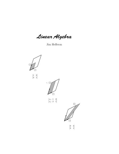
<strong>Linear</strong> <strong>Algebra</strong>Jim Hefferon( 13)( 21)∣ 1 23 1∣x 1 ·( 13)( 21)∣ x 1 · 1 2x 1 · 3 1∣( 68)( 21)∣ 6 28 1∣
NotationR, R + , R n real numbers, reals greater than 0, n-tuples of realsN natural numbers: {0, 1, 2, . . .}C complex numbers{. . . ∣ . . .} set of . . . such that . . .(a .. b), [a .. b] interval (open or closed) of reals between a and b〈. . .〉 sequence; like a set but order mattersV, W, U vector spaces⃗v, ⃗w vectors⃗0, ⃗0 V zero vector, zero vector of VB, D basesE n = 〈⃗e 1 , . . . , ⃗e n 〉 standard basis for R n⃗β, ⃗ δ basis vectorsRep B (⃗v) matrix representing the vectorP n set of n-th degree polynomialsM n×m set of n×m matrices[S] span of the set SM ⊕ N direct sum of subspacesV ∼ = W isomorphic spacesh, g homomorphisms, linear mapsH, G matricest, s transformations; maps from a space to itselfT, S square matricesRep B,D (h) matrix representing the map hh i,j matrix entry from row i, column j|T | determinant of the matrix TR(h), N (h) rangespace and nullspace of the map hR ∞ (h), N ∞ (h) generalized rangespace and nullspaceLower case Greek alphabetname character name character name characteralpha α iota ι rho ρbeta β kappa κ sigma σgamma γ lambda λ tau τdelta δ mu µ upsilon υepsilon ɛ nu ν phi φzeta ζ xi ξ chi χeta η omicron o psi ψtheta θ pi π omega ωCover. This is Cramer’s Rule for the system x 1 + 2x 2 = 6, 3x 1 + x 2 = 8. The size ofthe first box is the determinant shown (the absolute value of the size is the area). Thesize of the second box is x 1 times that, and equals the size of the final box. Hence, x 1is the final determinant divided by the first determinant.
PrefaceThis book helps students to master the material of a standard undergraduatelinear algebra course.The material is standard in that the topics covered are Gaussian reduction,vector spaces, linear maps, determinants, and eigenvalues and eigenvectors. Theaudience is also standard: sophmores or juniors, usually with a background ofat least one semester of Calculus and perhaps with as much as three semesters.The help that it gives to students comes from taking a developmental approach— this book’s presentation emphasizes motivation and naturalness, drivenhome by a wide variety of examples and extensive, careful, exercises. The developmentalapproach is what sets this book apart, so some expansion of theterm is appropriate here.Courses in the beginning of most Mathematics programs reward studentsless for understanding the theory and more for correctly applying formulas andalgorithms. Later courses ask for mathematical maturity: the ability to followdifferent types of arguments, a familiarity with the themes that underly manymathematical investigations like elementary set and function facts, and a capacityfor some independent reading and thinking. <strong>Linear</strong> algebra is an ideal spotto work on the transistion between the two kinds of courses. It comes early in aprogram so that progress made here pays off later, but also comes late enoughthat students are often majors and minors. The material is coherent, accessible,and elegant. There are a variety of argument styles — proofs by contradiction,if and only if statements, and proofs by induction, for instance — and examplesare plentiful.So, the aim of this book’s exposition is to help students develop from beingsuccessful at their present level, in classes where a majority of the members areinterested mainly in applications in science or engineering, to being successfulat the next level, that of serious students of the subject of mathematics itself.Helping students make this transition means taking the mathematics seriously,so all of the results in this book are proved. On the other hand, wecannot assume that students have already arrived, and so in contrast with moreabstract texts, we give many examples and they are often quite detailed.In the past, linear algebra texts commonly made this transistion abrubtly.They began with extensive computations of linear systems, matrix multiplications,and determinants. When the concepts — vector spaces and linear maps —finally appeared, and definitions and proofs started, often the change broughtstudents to a stop. In this book, while we start with a computational topic,iii
linear reduction, from the first we do more than compute. We do linear systemsquickly but completely, including the proofs needed to justify what we are computing.Then, with the linear systems work as motivation and at a point wherethe study of linear combinations seems natural, the second chapter starts withthe definition of a real vector space. This occurs by the end of the third week.Another example of our emphasis on motivation and naturalness is that thethird chapter on linear maps does not begin with the definition of homomorphism,but with that of isomorphism. That’s because this definition is easilymotivated by the observation that some spaces are “just like” others. Afterthat, the next section takes the reasonable step of defining homomorphism byisolating the operation-preservation idea. This approach loses mathematicalslickness, but it is a good trade because it comes in return for a large gain insensibility to students.One aim of a developmental approach is that students should feel throughoutthe presentation that they can see how the ideas arise, and perhaps picturethemselves doing the same type of work.The clearest example of the developmental approach taken here — and thefeature that most recommends this book — is the exercises. A student progressesmost while doing the exercises, so they have been selected with great care. Eachproblem set ranges from simple checks to resonably involved proofs. Since aninstructor usually assigns about a dozen exercises after each lecture, each sectionends with about twice that many, thereby providing a selection. There areeven a few problems that are challenging puzzles taken from various journals,competitions, or problems collections. (These are marked with a ‘?’ and aspart of the fun, the original wording has been retained as much as possible.)In total, the exercises are aimed to both build an ability at, and help studentsexperience the pleasure of, doing mathematics.Applications, and Computers. The point of view taken here, that linearalgebra is about vector spaces and linear maps, is not taken to the complete exclusionof others. Applications and the role of the computer are important andvital aspects of the subject. Consequently, each of this book’s chapters closeswith a few application or computer-related topics. Some are: network flows, thespeed and accuracy of computer linear reductions, Leontief Input/Output analysis,dimensional analysis, Markov chains, voting paradoxes, analytic projectivegeometry, and difference equations.These topics are brief enough to be done in a day’s class or to be given asindependent projects for individuals or small groups. Most simply give a readera taste of the subject, discuss how linear algebra comes in, point to some furtherreading, and give a few exercises. In short, these topics invite readers to see forthemselves that linear algebra is a tool that a professional must have.For people reading this book on their own. This book’s emphasis onmotivation and development make it a good choice for self-study. But, while aprofessional instructor can judge what pace and topics suit a class, if you arean independent student then perhaps you would find some advice helpful.Here are two timetables for a semester. The first focuses on core material.iv
the material, but it’s only that I have trouble with the problems” reveals a lackof understanding of what we are up to. Being able to do things with the ideasis their point. The quotes below express this sentiment admirably. They statewhat I believe is the key to both the beauty and the power of mathematics andthe sciences in general, and of linear algebra in particular (I took the liberty offormatting them as poems).I know of no better tacticthan the illustration of exciting principlesby well-chosen particulars.–Stephen Jay GouldIf you really wish to learnthen you must mount the machineand become acquainted with its tricksby actual trial.–Wilbur WrightJim HefferonMathematics, Saint Michael’s CollegeColchester, Vermont USA 05439http://joshua.smcvt.edu2006-May-20Author’s Note. Inventing a good exercise, one that enlightens as well as tests,is a creative act, and hard work. The inventor deserves recognition. But forsome reason texts have traditionally not given attributions for questions. I havechanged that here where I was sure of the source. I would greatly appreciatehearing from anyone who can help me to correctly attribute others of thequestions.vi
ContentsChapter One: <strong>Linear</strong> Systems 1I Solving <strong>Linear</strong> Systems . . . . . . . . . . . . . . . . . . . . . . . . 11 Gauss’ Method . . . . . . . . . . . . . . . . . . . . . . . . . . . 22 Describing the Solution Set . . . . . . . . . . . . . . . . . . . . 113 General = Particular + Homogeneous . . . . . . . . . . . . . . 20II <strong>Linear</strong> Geometry of n-Space . . . . . . . . . . . . . . . . . . . . . 321 Vectors in Space . . . . . . . . . . . . . . . . . . . . . . . . . . 322 Length and Angle Measures ∗ . . . . . . . . . . . . . . . . . . . 38III Reduced Echelon Form . . . . . . . . . . . . . . . . . . . . . . . . 461 Gauss-Jordan Reduction . . . . . . . . . . . . . . . . . . . . . . 462 Row Equivalence . . . . . . . . . . . . . . . . . . . . . . . . . . 52Topic: Computer <strong>Algebra</strong> Systems . . . . . . . . . . . . . . . . . . . 62Topic: Input-Output Analysis . . . . . . . . . . . . . . . . . . . . . . 64Topic: Accuracy of Computations . . . . . . . . . . . . . . . . . . . . 68Topic: Analyzing Networks . . . . . . . . . . . . . . . . . . . . . . . . 72Chapter Two: Vector Spaces 79I Definition of Vector Space . . . . . . . . . . . . . . . . . . . . . . 801 Definition and Examples . . . . . . . . . . . . . . . . . . . . . . 802 Subspaces and Spanning Sets . . . . . . . . . . . . . . . . . . . 91II <strong>Linear</strong> Independence . . . . . . . . . . . . . . . . . . . . . . . . . 1011 Definition and Examples . . . . . . . . . . . . . . . . . . . . . . 101III Basis and Dimension . . . . . . . . . . . . . . . . . . . . . . . . . 1121 Basis . . . . . . . . . . . . . . . . . . . . . . . . . . . . . . . . . 1122 Dimension . . . . . . . . . . . . . . . . . . . . . . . . . . . . . . 1183 Vector Spaces and <strong>Linear</strong> Systems . . . . . . . . . . . . . . . . 1234 Combining Subspaces ∗ . . . . . . . . . . . . . . . . . . . . . . . 130Topic: Fields . . . . . . . . . . . . . . . . . . . . . . . . . . . . . . . . 140Topic: Crystals . . . . . . . . . . . . . . . . . . . . . . . . . . . . . . 142Topic: Dimensional Analysis . . . . . . . . . . . . . . . . . . . . . . . 146vii
Chapter Three: Maps Between Spaces 153I Isomorphisms . . . . . . . . . . . . . . . . . . . . . . . . . . . . . 1531 Definition and Examples . . . . . . . . . . . . . . . . . . . . . . 1532 Dimension Characterizes Isomorphism . . . . . . . . . . . . . . 162II Homomorphisms . . . . . . . . . . . . . . . . . . . . . . . . . . . 1701 Definition . . . . . . . . . . . . . . . . . . . . . . . . . . . . . . 1702 Rangespace and Nullspace . . . . . . . . . . . . . . . . . . . . . 177III Computing <strong>Linear</strong> Maps . . . . . . . . . . . . . . . . . . . . . . . 1891 Representing <strong>Linear</strong> Maps with Matrices . . . . . . . . . . . . . 1892 Any Matrix Represents a <strong>Linear</strong> Map ∗ . . . . . . . . . . . . . . 199IV Matrix Operations . . . . . . . . . . . . . . . . . . . . . . . . . . 2061 Sums and Scalar Products . . . . . . . . . . . . . . . . . . . . . 2062 Matrix Multiplication . . . . . . . . . . . . . . . . . . . . . . . 2083 Mechanics of Matrix Multiplication . . . . . . . . . . . . . . . . 2164 Inverses . . . . . . . . . . . . . . . . . . . . . . . . . . . . . . . 225V Change of Basis . . . . . . . . . . . . . . . . . . . . . . . . . . . . 2321 Changing Representations of Vectors . . . . . . . . . . . . . . . 2322 Changing Map Representations . . . . . . . . . . . . . . . . . . 236VI Projection . . . . . . . . . . . . . . . . . . . . . . . . . . . . . . . 2441 Orthogonal Projection Into a Line ∗ . . . . . . . . . . . . . . . . 2442 Gram-Schmidt Orthogonalization ∗ . . . . . . . . . . . . . . . . 2483 Projection Into a Subspace ∗ . . . . . . . . . . . . . . . . . . . . 254Topic: Line of Best Fit . . . . . . . . . . . . . . . . . . . . . . . . . . 263Topic: Geometry of <strong>Linear</strong> Maps . . . . . . . . . . . . . . . . . . . . 268Topic: Markov Chains . . . . . . . . . . . . . . . . . . . . . . . . . . 275Topic: Orthonormal Matrices . . . . . . . . . . . . . . . . . . . . . . 281Chapter Four: Determinants 287I Definition . . . . . . . . . . . . . . . . . . . . . . . . . . . . . . . 2881 Exploration ∗ . . . . . . . . . . . . . . . . . . . . . . . . . . . . 2882 Properties of Determinants . . . . . . . . . . . . . . . . . . . . 2933 The Permutation Expansion . . . . . . . . . . . . . . . . . . . . 2974 Determinants Exist ∗ . . . . . . . . . . . . . . . . . . . . . . . . 306II Geometry of Determinants . . . . . . . . . . . . . . . . . . . . . . 3131 Determinants as Size Functions . . . . . . . . . . . . . . . . . . 313III Other Formulas . . . . . . . . . . . . . . . . . . . . . . . . . . . . 3201 Laplace’s Expansion ∗ . . . . . . . . . . . . . . . . . . . . . . . . 320Topic: Cramer’s Rule . . . . . . . . . . . . . . . . . . . . . . . . . . . 325Topic: Speed of Calculating Determinants . . . . . . . . . . . . . . . 328Topic: Projective Geometry . . . . . . . . . . . . . . . . . . . . . . . 331Chapter Five: Similarity 343I Complex Vector Spaces . . . . . . . . . . . . . . . . . . . . . . . . 3431 Factoring and Complex Numbers; A Review ∗ . . . . . . . . . . 3442 Complex Representations . . . . . . . . . . . . . . . . . . . . . 345II Similarity . . . . . . . . . . . . . . . . . . . . . . . . . . . . . . . 347viii
1 Definition and Examples . . . . . . . . . . . . . . . . . . . . . . 3472 Diagonalizability . . . . . . . . . . . . . . . . . . . . . . . . . . 3493 Eigenvalues and Eigenvectors . . . . . . . . . . . . . . . . . . . 353III Nilpotence . . . . . . . . . . . . . . . . . . . . . . . . . . . . . . . 3611 Self-Composition ∗ . . . . . . . . . . . . . . . . . . . . . . . . . 3612 Strings ∗ . . . . . . . . . . . . . . . . . . . . . . . . . . . . . . . 364IV Jordan Form . . . . . . . . . . . . . . . . . . . . . . . . . . . . . . 3751 Polynomials of Maps and Matrices ∗ . . . . . . . . . . . . . . . . 3752 Jordan Canonical Form ∗ . . . . . . . . . . . . . . . . . . . . . . 382Topic: Method of Powers . . . . . . . . . . . . . . . . . . . . . . . . . 395Topic: Stable Populations . . . . . . . . . . . . . . . . . . . . . . . . 399Topic: <strong>Linear</strong> Recurrences . . . . . . . . . . . . . . . . . . . . . . . . 401Appendix A-1Propositions . . . . . . . . . . . . . . . . . . . . . . . . . . . . . . . A-1Quantifiers . . . . . . . . . . . . . . . . . . . . . . . . . . . . . . . A-3Techniques of Proof . . . . . . . . . . . . . . . . . . . . . . . . . . A-5Sets, Functions, and Relations . . . . . . . . . . . . . . . . . . . . . A-7∗ Note: starred subsections are optional.ix
Chapter One<strong>Linear</strong> SystemsISolving <strong>Linear</strong> SystemsSystems of linear equations are common in science and mathematics. These twoexamples from high school science [Onan] give a sense of how they arise.The first example is from Physics. Suppose that we are given three objects,one with a mass known to be 2 kg, and are asked to find the unknown masses.Suppose further that experimentation with a meter stick produces these twobalances.40 50ch 2c25 502h1525Since the sum of moments on the left of each balance equals the sum of momentson the right (the moment of an object is its mass times its distance from thebalance point), the two balances give this system of two equations.40h + 15c = 10025c = 50 + 50hThe second example of a linear system is from Chemistry. We can mix,under controlled conditions, toluene C 7 H 8 and nitric acid HNO 3 to producetrinitrotoluene C 7 H 5 O 6 N 3 along with the byproduct water (conditions have tobe controlled very well, indeed — trinitrotoluene is better known as TNT). Inwhat proportion should those components be mixed? The number of atoms ofeach element present before the reactionx C 7 H 8 + y HNO 3 −→ z C 7 H 5 O 6 N 3 + w H 2 Omust equal the number present afterward. Applying that principle to the ele-1
2 Chapter One. <strong>Linear</strong> Systemsments C, H, N, and O in turn gives this system.7x = 7z8x + 1y = 5z + 2w1y = 3z3y = 6z + 1wTo finish each of these examples requires solving a system of equations. Ineach, the equations involve only the first power of the variables. This chaptershows how to solve any such system.I.1 Gauss’ Method1.1 Definition A linear equation in variables x 1 , x 2 , . . . , x n has the forma 1 x 1 + a 2 x 2 + a 3 x 3 + · · · + a n x n = dwhere the numbers a 1 , . . . , a n ∈ R are the equation’s coefficients and d ∈ Ris the constant. An n-tuple (s 1 , s 2 , . . . , s n ) ∈ R n is a solution of, or satisfies,that equation if substituting the numbers s 1 , . . . , s n for the variables gives atrue statement: a 1 s 1 + a 2 s 2 + . . . + a n s n = d.A system of linear equationsa 1,1 x 1 + a 1,2 x 2 + · · · + a 1,n x n = d 1a 2,1 x 1 + a 2,2 x 2 + · · · + a 2,n x n = d 2.a m,1 x 1 + a m,2 x 2 + · · · + a m,n x n = d mhas the solution (s 1 , s 2 , . . . , s n ) if that n-tuple is a solution of all of the equationsin the system.1.2 Example The ordered pair (−1, 5) is a solution of this system.In contrast, (5, −1) is not a solution.3x 1 + 2x 2 = 7−x 1 + x 2 = 6Finding the set of all solutions is solving the system. No guesswork or goodfortune is needed to solve a linear system. There is an algorithm that alwaysworks. The next example introduces that algorithm, called Gauss’ method. Ittransforms the system, step by step, into one with a form that is easily solved.
Section I. Solving <strong>Linear</strong> Systems 31.3 Example To solve this system3x 3 = 9x 1 + 5x 2 − 2x 3 = 213 x 1 + 2x 2 = 3we repeatedly transform it until it is in a form that is easy to solve.swap row 1 with row 3−→multiply row 1 by 3−→add −1 times row 1 to row 2−→13 x 1 + 2x 2 = 3x 1 + 5x 2 − 2x 3 = 23x 3 = 9x 1 + 6x 2 = 9x 1 + 5x 2 − 2x 3 = 23x 3 = 9x 1 + 6x 2 = 9−x 2 − 2x 3 = −73x 3 = 9The third step is the only nontrivial one. We’ve mentally multiplied both sidesof the first row by −1, mentally added that to the old second row, and writtenthe result in as the new second row.Now we can find the value of each variable. The bottom equation showsthat x 3 = 3. Substituting 3 for x 3 in the middle equation shows that x 2 = 1.Substituting those two into the top equation gives that x 1 = 3 and so the systemhas a unique solution: the solution set is { (3, 1, 3) }.Most of this subsection and the next one consists of examples of solvinglinear systems by Gauss’ method. We will use it throughout this book. It isfast and easy. But, before we get to those examples, we will first show thatthis method is also safe in that it never loses solutions or picks up extraneoussolutions.1.4 Theorem (Gauss’ method) If a linear system is changed to anotherby one of these operations(1) an equation is swapped with another(2) an equation has both sides multiplied by a nonzero constant(3) an equation is replaced by the sum of itself and a multiple of anotherthen the two systems have the same set of solutions.Each of those three operations has a restriction. Multiplying a row by 0 isnot allowed because obviously that can change the solution set of the system.Similarly, adding a multiple of a row to itself is not allowed because adding −1times the row to itself has the effect of multiplying the row by 0. Finally, swappinga row with itself is disallowed to make some results in the fourth chaptereasier to state and remember (and besides, self-swapping doesn’t accomplishanything).
4 Chapter One. <strong>Linear</strong> SystemsProof. We will cover the equation swap operation here and save the other twocases for Exercise 29.Consider this swap of row i with row j.a 1,1 x 1 + a 1,2 x 2 + · · · a 1,n x n = d 1 a 1,1 x 1 + a 1,2 x 2 + · · · a 1,n x n = d 1..a i,1 x 1 + a i,2 x 2 + · · · a i,n x n = d i a j,1 x 1 + a j,2 x 2 + · · · a j,n x n = d j. −→.a j,1 x 1 + a j,2 x 2 + · · · a j,n x n = d j a i,1 x 1 + a i,2 x 2 + · · · a i,n x n = d i..a m,1 x 1 + a m,2 x 2 + · · · a m,n x n = d m a m,1 x 1 + a m,2 x 2 + · · · a m,n x n = d mThe n-tuple (s 1 , . . . , s n ) satisfies the system before the swap if and only ifsubstituting the values, the s’s, for the variables, the x’s, gives true statements:a 1,1 s 1 +a 1,2 s 2 +· · ·+a 1,n s n = d 1 and . . . a i,1 s 1 +a i,2 s 2 +· · ·+a i,n s n = d i and . . .a j,1 s 1 + a j,2 s 2 + · · · + a j,n s n = d j and . . . a m,1 s 1 + a m,2 s 2 + · · · + a m,n s n = d m .In a requirement consisting of statements and-ed together we can rearrangethe order of the statements, so that this requirement is met if and only if a 1,1 s 1 +a 1,2 s 2 + · · · + a 1,n s n = d 1 and . . . a j,1 s 1 + a j,2 s 2 + · · · + a j,n s n = d j and . . .a i,1 s 1 + a i,2 s 2 + · · · + a i,n s n = d i and . . . a m,1 s 1 + a m,2 s 2 + · · · + a m,n s n = d m .This is exactly the requirement that (s 1 , . . . , s n ) solves the system after the rowswap.QED1.5 Definition The three operations from Theorem 1.4 are the elementaryreduction operations, or row operations, or Gaussian operations. They areswapping, multiplying by a scalar or rescaling, and pivoting.When writing out the calculations, we will abbreviate ‘row i’ by ‘ρ i ’. Forinstance, we will denote a pivot operation by kρ i + ρ j , with the row that ischanged written second. We will also, to save writing, often list pivot stepstogether when they use the same ρ i .1.6 Example A typical use of Gauss’ method is to solve this system.x + y = 02x − y + 3z = 3x − 2y − z = 3The first transformation of the system involves using the first row to eliminatethe x in the second row and the x in the third. To get rid of the second row’s2x, we multiply the entire first row by −2, add that to the second row, andwrite the result in as the new second row. To get rid of the third row’s x, wemultiply the first row by −1, add that to the third row, and write the result inas the new third row.x + y = 0−2ρ 1 +ρ 2−→ −3y + 3z = 3−ρ 1 +ρ 3−3y − z = 3
Section I. Solving <strong>Linear</strong> Systems 5(Note that the two ρ 1 steps −2ρ 1 + ρ 2 and −ρ 1 + ρ 3 are written as one operation.)In this second system, the last two equations involve only two unknowns.To finish we transform the second system into a third system, where the lastequation involves only one unknown. This transformation uses the second rowto eliminate y from the third row.x + y = 0−ρ 2 +ρ 3−→ −3y + 3z = 3−4z = 0Now we are set up for the solution. The third row shows that z = 0. Substitutethat back into the second row to get y = −1, and then substitute back into thefirst row to get x = 1.1.7 Example For the Physics problem from the start of this chapter, Gauss’method gives this.40h + 15c = 100−50h + 25c = 505/4ρ 1+ρ 2−→40h + 15c = 100(175/4)c = 175So c = 4, and back-substitution gives that h = 1. (The Chemistry problem issolved later.)1.8 Example The reductionx + y + z = 92x + 4y − 3z = 13x + 6y − 5z = 0x + y + z = 9−2ρ 1 +ρ 2−→ 2y − 5z = −17−3ρ 1+ρ 33y − 8z = −27−(3/2)ρ 2 +ρ 3−→x + y + z = 92y − 5z = −17−(1/2)z = −(3/2)shows that z = 3, y = −1, and x = 7.As these examples illustrate, Gauss’ method uses the elementary reductionoperations to set up back-substitution.1.9 Definition In each row, the first variable with a nonzero coefficient is therow’s leading variable. A system is in echelon form if each leading variable isto the right of the leading variable in the row above it (except for the leadingvariable in the first row).1.10 Example The only operation needed in the examples above is pivoting.Here is a linear system that requires the operation of swapping equations. Afterthe first pivotx − y = 02x − 2y + z + 2w = 4y + w = 02z + w = 5−→z + 2w = 4y + w = 0x − y = 02z + w = 5−2ρ 1 +ρ 2
6 Chapter One. <strong>Linear</strong> Systemsthe second equation has no leading y. To get one, we look lower down in thesystem for a row that has a leading y and swap it in.−→y + w = 0z + 2w = 4x − y = 02z + w = 5ρ 2↔ρ 3(Had there been more than one row below the second with a leading y then wecould have swapped in any one.) The rest of Gauss’ method goes as before.x − y = 0y + w = 0−→z + 2w = 4−3w = −3−2ρ 3+ρ 4Back-substitution gives w = 1, z = 2 , y = −1, and x = −1.Strictly speaking, the operation of rescaling rows is not needed to solve linearsystems. We have included it because we will use it later in this chapter as partof a variation on Gauss’ method, the Gauss-Jordan method.All of the systems seen so far have the same number of equations as unknowns.All of them have a solution, and for all of them there is only onesolution. We finish this subsection by seeing for contrast some other things thatcan happen.1.11 Example <strong>Linear</strong> systems need not have the same number of equationsas unknowns. This systemx + 3y = 12x + y = −32x + 2y = −2has more equations than variables.system also, since thisGauss’ method helps us understand thisx + 3y = 1−2ρ 1 +ρ 2−→ −5y = −5−2ρ 1+ρ 3−4y = −4shows that one of the equations is redundant. Echelon form−(4/5)ρ 2 +ρ 3−→x + 3y = 1−5y = −50 = 0gives y = 1 and x = −2. The ‘0 = 0’ is derived from the redundancy.That example’s system has more equations than variables. Gauss’ methodis also useful on systems with more variables than equations. Many examplesare in the next subsection.
Section I. Solving <strong>Linear</strong> Systems 7Another way that linear systems can differ from the examples shown earlieris that some linear systems do not have a unique solution. This can happen intwo ways.The first is that it can fail to have any solution at all.1.12 Example Contrast the system in the last example with this one.x + 3y = 12x + y = −32x + 2y = 0x + 3y = 1−2ρ 1 +ρ 2−→ −5y = −5−2ρ 1 +ρ 3−4y = −2Here the system is inconsistent: no pair of numbers satisfies all of the equationssimultaneously. Echelon form makes this inconsistency obvious.The solution set is empty.−(4/5)ρ 2+ρ 3−→x + 3y = 1−5y = −50 = 21.13 Example The prior system has more equations than unknowns, but thatis not what causes the inconsistency — Example 1.11 has more equations thanunknowns and yet is consistent. Nor is having more equations than unknownsnecessary for inconsistency, as is illustrated by this inconsistent system with thesame number of equations as unknowns.x + 2y = 82x + 4y = 8−2ρ 1+ρ 2−→x + 2y = 80 = −8The other way that a linear system can fail to have a unique solution is tohave many solutions.1.14 Example In this systemx + y = 42x + 2y = 8any pair of numbers satisfying the first equation automatically satisfies the second.The solution set {(x, y) ∣ x + y = 4} is infinite; some of its membersare (0, 4), (−1, 5), and (2.5, 1.5). The result of applying Gauss’ method herecontrasts with the prior example because we do not get a contradictory equation.−2ρ 1 +ρ 2−→x + y = 40 = 0Don’t be fooled by the ‘0 = 0’ equation in that example. It is not the signalthat a system has many solutions.
8 Chapter One. <strong>Linear</strong> Systems1.15 Example The absence of a ‘0 = 0’ does not keep a system from havingmany different solutions. This system is in echelon formx + y + z = 0y + z = 0has no ‘0 = 0’, and yet has infinitely many solutions. (For instance, each ofthese is a solution: (0, 1, −1), (0, 1/2, −1/2), (0, 0, 0), and (0, −π, π). There areinfinitely many solutions because any triple whose first component is 0 andwhose second component is the negative of the third is a solution.)Nor does the presence of a ‘0 = 0’ mean that the system must have manysolutions. Example 1.11 shows that. So does this system, which does not havemany solutions — in fact it has none — despite that when it is brought to echelonform it has a ‘0 = 0’ row.2x − 2z = 6y + z = 12x + y − z = 73y + 3z = 0−→y + z = 1y + z = 12x − 2z = 63y + 3z = 0−ρ 1 +ρ 32x − 2z = 6−ρ 2 +ρ 3 y + z = 1−→−3ρ 2 +ρ 4 0 = 00 = −3We will finish this subsection with a summary of what we’ve seen so farabout Gauss’ method.Gauss’ method uses the three row operations to set a system up for backsubstitution. If any step shows a contradictory equation then we can stopwith the conclusion that the system has no solutions. If we reach echelon formwithout a contradictory equation, and each variable is a leading variable in itsrow, then the system has a unique solution and we find it by back substitution.Finally, if we reach echelon form without a contradictory equation, and there isnot a unique solution (at least one variable is not a leading variable) then thesystem has many solutions.The next subsection deals with the third case — we will see how to describethe solution set of a system with many solutions.Exerciseš 1.16 Use Gauss’ method to find the unique solution for each system.x − z = 02x + 3y = 13(a) (b) 3x + y = 1x − y = −1−x + y + z = 4̌ 1.17 Use Gauss’ method to solve each system or conclude ‘many solutions’ or ‘nosolutions’.
Section I. Solving <strong>Linear</strong> Systems 9(a) 2x + 2y = 5x − 4y = 0(b) −x + y = 1x + y = 2(c) x − 3y + z = 1x + y + 2z = 14(d) −x − y = 1 (e) 4y + z = 20 (f) 2x + z + w = 5−3x − 3y = 2 2x − 2y + z = 0y − w = −1x + z = 5 3x − z − w = 0x + y − z = 10 4x + y + 2z + w = 9̌ 1.18 There are methods for solving linear systems other than Gauss’ method. Oneoften taught in high school is to solve one of the equations for a variable, thensubstitute the resulting expression into other equations. That step is repeateduntil there is an equation with only one variable. From that, the first numberin the solution is derived, and then back-substitution can be done. This methodtakes longer than Gauss’ method, since it involves more arithmetic operations,and is also more likely to lead to errors. To illustrate how it can lead to wrongconclusions, we will use the systemx + 3y = 12x + y = −32x + 2y = 0from Example 1.12.(a) Solve the first equation for x and substitute that expression into the secondequation. Find the resulting y.(b) Again solve the first equation for x, but this time substitute that expressioninto the third equation. Find this y.What extra step must a user of this method take to avoid erroneously concludinga system has a solution?̌ 1.19 For which values of k are there no solutions, many solutions, or a uniquesolution to this system?x − y = 13x − 3y = ǩ 1.20 This system is not linear, in some sense,2 sin α − cos β + 3 tan γ = 34 sin α + 2 cos β − 2 tan γ = 106 sin α − 3 cos β + tan γ = 9and yet we can nonetheless apply Gauss’ method. Do so. Does the system have asolution?̌ 1.21 What conditions must the constants, the b’s, satisfy so that each of thesesystems has a solution? Hint. Apply Gauss’ method and see what happens to theright side. [Anton](a) x − 3y = b 1 (b) x 1 + 2x 2 + 3x 3 = b 13x + y = b 2 2x 1 + 5x 2 + 3x 3 = b 2x + 7y = b 3 x 1 + 8x 3 = b 32x + 4y = b 41.22 True or false: a system with more unknowns than equations has at least onesolution. (As always, to say ‘true’ you must prove it, while to say ‘false’ you mustproduce a counterexample.)1.23 Must any Chemistry problem like the one that starts this subsection — a balancethe reaction problem — have infinitely many solutions?̌ 1.24 Find the coefficients a, b, and c so that the graph of f(x) = ax 2 +bx+c passesthrough the points (1, 2), (−1, 6), and (2, 3).
10 Chapter One. <strong>Linear</strong> Systems1.25 Gauss’ method works by combining the equations in a system to make newequations.(a) Can the equation 3x−2y = 5 be derived, by a sequence of Gaussian reductionsteps, from the equations in this system?x + y = 14x − y = 6(b) Can the equation 5x−3y = 2 be derived, by a sequence of Gaussian reductionsteps, from the equations in this system?2x + 2y = 53x + y = 4(c) Can the equation 6x − 9y + 5z = −2 be derived, by a sequence of Gaussianreduction steps, from the equations in the system?2x + y − z = 46x − 3y + z = 51.26 Prove that, where a, b, . . . , e are real numbers and a ≠ 0, ifhas the same solution set asax + by = cax + dy = ethen they are the same equation. What if a = 0?̌ 1.27 Show that if ad − bc ≠ 0 thenhas a unique solution.̌ 1.28 In the systemax + by = jcx + dy = kax + by = cdx + ey = feach of the equations describes a line in the xy-plane. By geometrical reasoning,show that there are three possibilities: there is a unique solution, there is nosolution, and there are infinitely many solutions.1.29 Finish the proof of Theorem 1.4.1.30 Is there a two-unknowns linear system whose solution set is all of R 2 ?̌ 1.31 Are any of the operations used in Gauss’ method redundant? That is, canany of the operations be synthesized from the others?1.32 Prove that each operation of Gauss’ method is reversible. That is, show that iftwo systems are related by a row operation S 1 → S 2 then there is a row operationto go back S 2 → S 1 .? 1.33 A box holding pennies, nickels and dimes contains thirteen coins with a totalvalue of 83 cents. How many coins of each type are in the box? [Anton]? 1.34 Four positive integers are given. Select any three of the integers, find theirarithmetic average, and add this result to the fourth integer. Thus the numbers29, 23, 21, and 17 are obtained. One of the original integers is:
Section I. Solving <strong>Linear</strong> Systems 11(a) 19 (b) 21 (c) 23 (d) 29 (e) 17[Con. Prob. 1955]? ̌ 1.35 Laugh at this: AHAHA + TEHE = TEHAW. It resulted from substitutinga code letter for each digit of a simple example in addition, and it is required toidentify the letters and prove the solution unique. [Am. Math. Mon., Jan. 1935]? 1.36 The Wohascum County Board of Commissioners, which has 20 members, recentlyhad to elect a President. There were three candidates (A, B, and C); oneach ballot the three candidates were to be listed in order of preference, with noabstentions. It was found that 11 members, a majority, preferred A over B (thusthe other 9 preferred B over A). Similarly, it was found that 12 members preferredC over A. Given these results, it was suggested that B should withdraw, to enablea runoff election between A and C. However, B protested, and it was then foundthat 14 members preferred B over C! The Board has not yet recovered from the resultingconfusion. Given that every possible order of A, B, C appeared on at leastone ballot, how many members voted for B as their first choice? [Wohascum no. 2]? 1.37 “This system of n linear equations with n unknowns,” said the Great Mathematician,“has a curious property.”“Good heavens!” said the Poor Nut, “What is it?”“Note,” said the Great Mathematician, “that the constants are in arithmeticprogression.”“It’s all so clear when you explain it!” said the Poor Nut. “Do you mean like6x + 9y = 12 and 15x + 18y = 21?”“Quite so,” said the Great Mathematician, pulling out his bassoon. “Indeed,the system has a unique solution. Can you find it?”“Good heavens!” cried the Poor Nut, “I am baffled.”Are you? [Am. Math. Mon., Jan. 1963]I.2 Describing the Solution SetA linear system with a unique solution has a solution set with one element. Alinear system with no solution has a solution set that is empty. In these casesthe solution set is easy to describe. Solution sets are a challenge to describeonly when they contain many elements.2.1 Example This system has many solutions because in echelon form2x + z = 3x − y − z = 13x − y = 42x + z = 3−(1/2)ρ 1+ρ 2−→ −y − (3/2)z = −1/2−(3/2)ρ 1 +ρ 3−y − (3/2)z = −1/2−ρ 2+ρ 3−→2x + z = 3−y − (3/2)z = −1/20 = 0not all of the variables are leading variables. The Gauss’ method theoremshowed that a triple satisfies the first system if and only if it satisfies the third.Thus, the solution set {(x, y, z) ∣ 2x + z = 3 and x − y − z = 1 and 3x − y = 4}
12 Chapter One. <strong>Linear</strong> Systemscan also be described as {(x, y, z) ∣ 2x + z = 3 and −y − 3z/2 = −1/2}. However,this second description is not much of an improvement. It has two equationsinstead of three, but it still involves some hard-to-understand interactionamong the variables.To get a description that is free of any such interaction, we take the variablethat does not lead any equation, z, and use it to describe the variablesthat do lead, x and y. The second equation gives y = (1/2) − (3/2)z andthe first equation gives x = (3/2) − (1/2)z. Thus, the solution set can be describedas {(x, y, z) = ((3/2) − (1/2)z, (1/2) − (3/2)z, z) ∣ z ∈ R}. For instance,(1/2, −5/2, 2) is a solution because taking z = 2 gives a first component of 1/2and a second component of −5/2.The advantage of this description over the ones above is that the only variableappearing, z, is unrestricted — it can be any real number.2.2 Definition The non-leading variables in an echelon-form linear systemare free variables.In the echelon form system derived in the above example, x and y are leadingvariables and z is free.2.3 Example A linear system can end with more than one variable free. Thisrow reductionx + y + z − w = 1y − z + w = −13x + 6z − 6w = 6−y + z − w = 1−→y − z + w = −1−3y + 3z − 3w = 3x + y + z − w = 1−y + z − w = 1−3ρ 1 +ρ 33ρ 2 +ρ 3 y − z + w = −1−→ρ 2 +ρ 4 0 = 0x + y + z − w = 10 = 0ends with x and y leading, and with both z and w free. To get the descriptionthat we prefer we will start at the bottom. We first express y in terms ofthe free variables z and w with y = −1 + z − w. Next, moving up to thetop equation, substituting for y in the first equation x + (−1 + z − w) + z −w = 1 and solving for x yields x = 2 − 2z + 2w. Thus, the solution set is{2 − 2z + 2w, −1 + z − w, z, w) ∣ z, w ∈ R}.We prefer this description because the only variables that appear, z and w,are unrestricted. This makes the job of deciding which four-tuples are systemsolutions into an easy one. For instance, taking z = 1 and w = 2 gives thesolution (4, −2, 1, 2). In contrast, (3, −2, 1, 2) is not a solution, since the firstcomponent of any solution must be 2 minus twice the third component plustwice the fourth.
Section I. Solving <strong>Linear</strong> Systems 132.4 Example After this reduction2x − 2y = 0z + 3w = 23x − 3y = 0x − y + 2z + 6w = 4−(3/2)ρ 1+ρ 3z + 3w = 2−→−(1/2)ρ 1+ρ 40 = 02x − 2y = 02z + 6w = 4−→z + 3w = 20 = 02x − 2y = 00 = 0−2ρ 2+ρ 4x and z lead, y and w are free. The solution set is {(y, y, 2 − 3w, w) ∣ ∣ y, w ∈ R}.For instance, (1, 1, 2, 0) satisfies the system — take y = 1 and w = 0. The fourtuple(1, 0, 5, 4) is not a solution since its first coordinate does not equal itssecond.We refer to a variable used to describe a family of solutions as a parameterand we say that the set above is parametrized with y and w. (The terms‘parameter’ and ‘free variable’ do not mean the same thing. Above, y and ware free because in the echelon form system they do not lead any row. Theyare parameters because they are used in the solution set description. We couldhave instead parametrized with y and z by rewriting the second equation asw = 2/3 − (1/3)z. In that case, the free variables are still y and w, but theparameters are y and z. Notice that we could not have parametrized with x andy, so there is sometimes a restriction on the choice of parameters. The terms‘parameter’ and ‘free’ are related because, as we shall show later in this chapter,the solution set of a system can always be parametrized with the free variables.Consequently, we shall parametrize all of our descriptions in this way.)2.5 Example This is another system with infinitely many solutions.x + 2y = 12x + z = 23x + 2y + z − w = 4x + 2y = 1−2ρ 1 +ρ 2−→ −4y + z = 0−3ρ 1 +ρ 3−4y + z − w = 1x + 2y = 1−ρ 2 +ρ 3−→ −4y + z = 0−w = 1The leading variables are x, y, and w. The variable z is free. (Notice here that,although there are infinitely many solutions, the value of one of the variables isfixed — w = −1.) Write w in terms of z with w = −1 + 0z. Then y = (1/4)z.To express x in terms of z, substitute for y into the first equation to get x =1 − (1/2)z. The solution set is {(1 − (1/2)z, (1/4)z, z, −1) ∣ ∣ z ∈ R}.We finish this subsection by developing the notation for linear systems andtheir solution sets that we shall use in the rest of this book.2.6 Definition An m×n matrix is a rectangular array of numbers with m rowsand n columns. Each number in the matrix is an entry,
14 Chapter One. <strong>Linear</strong> SystemsMatrices are usually named by upper case roman letters, e.g. A. Each entry isdenoted by the corresponding lower-case letter, e.g. a i,j is the number in row iand column j of the array. For instance,( )1 2.2 5A =3 4 −7has two rows and three columns, and so is a 2×3 matrix. (Read that “twoby-three”;the number of rows is always stated first.) The entry in the secondrow and first column is a 2,1 = 3. Note that the order of the subscripts matters:a 1,2 ≠ a 2,1 since a 1,2 = 2.2. (The parentheses around the array are a typographicdevice so that when two matrices are side by side we can tell where oneends and the other starts.)Matrices occur throughout this book. We shall use M n×m to denote thecollection of n×m matrices.2.7 Example We can abbreviate this linear systemwith this matrix.x 1 + 2x 2 = 4x 2 − x 3 = 0x 1 + 2x 3 = 4⎛⎝ 1 2 0 4⎞0 1 −1 0⎠1 0 2 4The vertical bar just reminds a reader of the difference between the coefficientson the systems’s left hand side and the constants on the right. When a baris used to divide a matrix into parts, we call it an augmented matrix. In thisnotation, Gauss’ method goes this way.⎛⎝ 1 2 0 4⎞ ⎛0 1 −1 0⎠ −ρ 1+ρ 3−→ ⎝ 1 2 0 4⎞ ⎛0 1 −1 0⎠ 2ρ 2+ρ 3−→ ⎝ 1 2 0 4⎞0 1 −1 0⎠1 0 2 40 −2 2 0 0 0 0 0The second row stands for y − z = 0 and the first row stands for x + 2y = 4 sothe solution set is {(4 − 2z, z, z) ∣ ∣ z ∈ R}. One advantage of the new notation isthat the clerical load of Gauss’ method — the copying of variables, the writingof +’s and =’s, etc. — is lighter.We will also use the array notation to clarify the descriptions of solutionsets. A description like {(2 − 2z + 2w, −1 + z − w, z, w) ∣ z, w ∈ R} from Example2.3 is hard to read. We will rewrite it to group all the constants together,all the coefficients of z together, and all the coefficients of w together. We willwrite them vertically, in one-column wide matrices.⎛ ⎞ ⎛ ⎞ ⎛ ⎞2 −2 2{ ⎜−1⎟⎝ 0 ⎠ + ⎜ 1⎟⎝ 1 ⎠ · z + ⎜−1⎟⎝ 0 ⎠ · w ∣ z, w ∈ R}0 0 1
Section I. Solving <strong>Linear</strong> Systems 15For instance, the top line says that x = 2 − 2z + 2w. The next section gives ageometric interpretation that will help us picture the solution sets when theyare written in this way.2.8 Definition A vector (or column vector) is a matrix with a single column.A matrix with a single row is a row vector. The entries of a vector are itscomponents.Vectors are an exception to the convention of representing matrices withcapital roman letters. We use lower-case roman or greek letters overlined withan arrow: ⃗a, ⃗ b, . . . or ⃗α, β, ⃗ . . . (boldface is also common: a or α). For instance,this is a column vector with a third component of 7.⎛ ⎞⃗v = ⎝ 1 3⎠72.9 Definition The linear equation a 1 x 1 + a 2 x 2 + · · · + a n x n = d withunknowns x 1 , . . . , x n is satisfied by⎛ ⎞s 1⎜⃗s = . ⎟⎝ . ⎠s nif a 1 s 1 + a 2 s 2 + · · · + a n s n = d. A vector satisfies a linear system if it satisfieseach equation in the system.The style of description of solution sets that we use involves adding thevectors, and also multiplying them by real numbers, such as the z and w. Weneed to define these operations.2.10 Definition The vector sum of ⃗u and ⃗v is this.⎛ ⎞ ⎛ ⎞ ⎛ ⎞u 1 v 1 u 1 + v 1⎜⃗u + ⃗v = . ⎟ ⎜⎝ . ⎠ + . ⎟ ⎜⎝ . ⎠ =. ⎟⎝ . ⎠u n v n u n + v nIn general, two matrices with the same number of rows and the same numberof columns add in this way, entry-by-entry.2.11 Definition The scalar multiplication of the real number r and the vector⃗v is this.⎛ ⎞ ⎛ ⎞v 1 rv 1⎜r · ⃗v = r · ⎝⎟ ⎜. ⎠ = ⎝⎟. ⎠v n rv nIn general, any matrix is multiplied by a real number in this entry-by-entryway.
16 Chapter One. <strong>Linear</strong> SystemsScalar multiplication can be written in either order: r · ⃗v or ⃗v · r, or withoutthe ‘·’ symbol: r⃗v. (Do not refer to scalar multiplication as ‘scalar product’because that name is used for a different operation.)2.12 Example⎛⎝ 2 31⎞⎠ +⎛⎝ 3 ⎞ ⎛−1⎠ = ⎝ 2 + 3⎞ ⎛3 − 1⎠ = ⎝ 5 ⎞2⎠ 7 ·4 1 + 4 5⎛ ⎞ ⎛ ⎞1 7⎜ 4⎟⎝−1⎠ = ⎜ 28⎟⎝ −7 ⎠−3 −21Notice that the definitions of vector addition and scalar multiplication agreewhere they overlap, for instance, ⃗v + ⃗v = 2⃗v.With the notation defined, we can now solve systems in the way that we willuse throughout this book.2.13 Example This system2x + y − w = 4y + w + u = 4x − z + 2w = 0reduces in this way.⎛⎝ 2 1 0 −1 0 4⎞0 1 0 1 1 4⎠1 0 −1 2 0 0−(1/2)ρ1+ρ3−→(1/2)ρ 2+ρ 3−→⎛⎝ 2 1 0 −1 0 4⎞0 1 0 1 1 4 ⎠0 −1/2 −1 5/2 0 −2⎛⎝ 2 1 0 −1 0 4⎞0 1 0 1 1 4⎠0 0 −1 3 1/2 0The solution set is {(w + (1/2)u, 4 − w − u, 3w + (1/2)u, w, u) ∣ w, u ∈ R}. Wewrite that in vector form.⎛ ⎞ ⎛ ⎞ ⎛ ⎞ ⎛ ⎞x 0 1 1/2y{⎜z⎟⎝w⎠ = 4⎜0⎟⎝0⎠ + −1⎜ 3⎟⎝ 1 ⎠ w + −1⎜1/2⎟⎝ 0 ⎠ u ∣ w, u ∈ R}u 0 0 1Note again how well vector notation sets off the coefficients of each parameter.For instance, the third row of the vector form shows plainly that if u is heldfixed then z increases three times as fast as w.That format also shows plainly that there are infinitely many solutions. Forexample, we can fix u as 0, let w range over the real numbers, and consider thefirst component x. We get infinitely many first components and hence infinitelymany solutions.
Section I. Solving <strong>Linear</strong> Systems 17Another thing shown plainly is that setting both w and u to zero gives thatthis⎛ ⎞ ⎛ ⎞x 0y⎜z⎟⎝w⎠ = 4⎜0⎟⎝0⎠u 0is a particular solution of the linear system.2.14 Example In the same way, this systemreduces⎛⎝ 1 −1 1 1⎞3 0 1 35 −2 3 5⎛⎠ −3ρ 1+ρ 2−→−5ρ 1+ρ 3x − y + z = 13x + z = 35x − 2y + 3z = 5⎝ 1 −1 1 1⎞0 3 −2 00 3 −2 0⎠ −ρ 2+ρ 3−→to a one-parameter solution set.⎛ ⎞ ⎛ ⎞{ ⎝ 1 0⎠ + ⎝ −1/32/3 ⎠ z ∣ z ∈ R}0 1⎛⎝ 1 −1 1 1⎞0 3 −2 0⎠0 0 0 0Before the exercises, we pause to point out some things that we have yet todo.The first two subsections have been on the mechanics of Gauss’ method.Except for one result, Theorem 1.4 — without which developing the methoddoesn’t make sense since it says that the method gives the right answers — wehave not stopped to consider any of the interesting questions that arise.For example, can we always describe solution sets as above, with a particularsolution vector added to an unrestricted linear combination of some other vectors?The solution sets we described with unrestricted parameters were easilyseen to have infinitely many solutions so an answer to this question could tellus something about the size of solution sets. An answer to that question couldalso help us picture the solution sets, in R 2 , or in R 3 , etc.Many questions arise from the observation that Gauss’ method can be donein more than one way (for instance, when swapping rows, we may have a choiceof which row to swap with). Theorem 1.4 says that we must get the samesolution set no matter how we proceed, but if we do Gauss’ method in twodifferent ways must we get the same number of free variables both times, sothat any two solution set descriptions have the same number of parameters?Must those be the same variables (e.g., is it impossible to solve a problem oneway and get y and w free or solve it another way and get y and z free)?
18 Chapter One. <strong>Linear</strong> SystemsIn the rest of this chapter we answer these questions. The answer to eachis ‘yes’. The first question is answered in the last subsection of this section. Inthe second section we give a geometric description of solution sets. In the finalsection of this chapter we tackle the last set of questions. Consequently, by theend of the first chapter we will not only have a solid grounding in the practiceof Gauss’ method, we will also have a solid grounding in the theory. We will besure of what can and cannot happen in a reduction.Exerciseš 2.15 Find the indicated entry of the matrix, if it is defined.( )1 3 1A =2 −1 4(a) a 2,1 (b) a 1,2 (c) a 2,2 (d) a 3,1̌ 2.16 Give the size of each matrix.( ) ( ) 1 1 ( )1 0 45 10(a)(b) −1 1 (c)2 1 510 53 −1̌ 2.17 Do the indicated vector operation, if it is defined.( ) ( ) 2 3 ( ) ( ) ( ) 1 3 4(a) 1 + 0 (b) 5 (c) 5 − 1−11 41 1( )) ) )12)(e)+( 123(f) 6( 311− 4( 203( 1+ 2 15Express the solution using vec-̌ 2.18 Solve each system using matrix notation.tors.(a) 3x + 6y = 18 (b) x + y = 1x + 2y = 6 x − y = −1(d) 2a + b − c = 22a + c = 3a − b = 0(e) x + 2y − z = 32x + y + w = 4x − y + z + w = 1̌ 2.19 Solve each system using matrix notation.notation.(a) 2x + y − z = 1 (b) x − z = 14x − y = 3y + 2z − w = 3x + 2y + 3z − w = 7(d) 7(21)+ 9(35)(c) x 1 + x 3 = 4x 1 − x 2 + 2x 3 = 54x 1 − x 2 + 5x 3 = 17(f) x + z + w = 42x + y − w = 23x + y + z = 7Give each solution set in vector(c) x − y + z = 0y + w = 03x − 2y + 3z + w = 0−y − w = 0(d) a + 2b + 3c + d − e = 13a − b + c + d + e = 3̌ 2.20 The vector is in the set. What value of the parameters produces that vector?( ) ( )5 1 ∣ (a) , { k k ∈ R}−5 −1) ( ) )−2(b)( −121, {10i +( 301j ∣ ∣ i, j ∈ R}
Section I. Solving <strong>Linear</strong> Systems 19( ) ) ( )0 1 2(c) −4 , {( ∣ 1 m + 0 n m, n ∈ R}2 0 12.21 Decide ( ) if the ( vector ) is in the set.3 −6 ∣ (a) , { k k ∈ R}−1 2( ( )5 5(b) , {4)∣ j j ∈ R}−4( ) ) ( )2 0 1(c) 1 , {( ∣ 3 + −1 r r ∈ R}−1)−7)3)( ( 1 2 −3(d) 0 , {(0 j + −1∣ k j, k ∈ R}1 1 12.22 Parametrize the solution set of this one-equation system.x 1 + x 2 + · · · + x n = 0̌ 2.23 (a) Apply Gauss’ method to the left-hand side to solvex + 2y − w = a2x + z = bx + y + 2w = cfor x, y, z, and w, in terms of the constants a, b, and c.(b) Use your answer from the prior part to solve this.x + 2y − w = 32x + z = 1x + y + 2w = −2̌ 2.24 Why is the comma needed in the notation ‘a i,j’ for matrix entries?̌ 2.25 Give the 4×4 matrix whose i, j-th entry is(a) i + j; (b) −1 to the i + j power.2.26 For any matrix A, the transpose of A, written A trans , is the matrix whosecolumns are the rows of A. Find the transpose of each of these.( ) ( ) ( )1 2 32 −35 10(a)(b)(c)(d)4 5 61 110 5( ) 110̌ 2.27 (a) Describe all functions f(x) = ax 2 + bx + c such that f(1) = 2 andf(−1) = 6.(b) Describe all functions f(x) = ax 2 + bx + c such that f(1) = 2.2.28 Show that any set of five points from the plane R 2 lie on a common conicsection, that is, they all satisfy some equation of the form ax 2 + by 2 + cxy + dx +ey + f = 0 where some of a, . . . , f are nonzero.2.29 Make up a four equations/four unknowns system having(a) a one-parameter solution set;(b) a two-parameter solution set;(c) a three-parameter solution set.? 2.30 (a) Solve the system of equations.ax + y = a 2x + ay = 1For what values of a does the system fail to have solutions, and for what valuesof a are there infinitely many solutions?
20 Chapter One. <strong>Linear</strong> Systems(b) Answer the above question for the system.ax + y = a 3x + ay = 1[USSR Olympiad no. 174]? 2.31 In air a gold-surfaced sphere weighs 7588 grams. It is known that it maycontain one or more of the metals aluminum, copper, silver, or lead. When weighedsuccessively under standard conditions in water, benzene, alcohol, and glycerineits respective weights are 6588, 6688, 6778, and 6328 grams. How much, if any,of the forenamed metals does it contain if the specific gravities of the designatedsubstances are taken to be as follows?Aluminum 2.7 Alcohol 0.81Copper 8.9 Benzene 0.90Gold 19.3 Glycerine 1.26Lead 11.3 Water 1.00Silver 10.8[Math. Mag., Sept. 1952]I.3 General = Particular + HomogeneousThe prior subsection has many descriptions of solution sets. They all fit apattern. They have a vector that is a particular solution of the system addedto an unrestricted combination of some other vectors. The solution set fromExample 2.13 illustrates.⎛ ⎞ ⎛ ⎞ ⎛ ⎞0 1 1/24⎟ −1{⎜0⎟ + w⎜ 3⎟⎝0⎠⎝ 1 ⎠ + u −1⎜1/2∣⎟ w, u ∈ R}⎝ 0 ⎠0} {{ } }0{{1}particularsolutionunrestrictedcombinationThe combination is unrestricted in that w and u can be any real numbers —there is no condition like “such that 2w −u = 0” that would restrict which pairsw, u can be used to form combinations.That example shows an infinite solution set conforming to the pattern. Wecan think of the other two kinds of solution sets as also fitting the same pattern.A one-element solution set fits in that it has a particular solution, andthe unrestricted combination part is a trivial sum (that is, instead of being acombination of two vectors, as above, or a combination of one vector, it is acombination of no vectors). A zero-element solution set fits the pattern sincethere is no particular solution, and so the set of sums of that form is empty.We will show that the examples from the prior subsection are representative,in that the description pattern discussed above holds for every solution set.
Section I. Solving <strong>Linear</strong> Systems 213.1 Theorem For any linear system there are vectors ⃗ β 1 , . . . , ⃗ β k such thatthe solution set can be described as{⃗p + c 1⃗ β1 + · · · + c k⃗ βk∣ ∣ c 1 , . . . , c k ∈ R}where ⃗p is any particular solution, and where the system has k free variables.This description has two parts, the particular solution ⃗p and also the unrestrictedlinear combination of the β’s. ⃗ We shall prove the theorem in twocorresponding parts, with two lemmas.We will focus first on the unrestricted combination part. To do that, weconsider systems that have the vector of zeroes as one of the particular solutions,so that ⃗p + c 1β1 ⃗ + · · · + c kβk ⃗ can be shortened to c 1β1 ⃗ + · · · + c kβk ⃗ .3.2 Definition A linear equation is homogeneous if it has a constant of zero,that is, if it can be put in the form a 1 x 1 + a 2 x 2 + · · · + a n x n = 0.(These are ‘homogeneous’ because all of the terms involve the same power oftheir variable — the first power — including a ‘0x 0 ’ that we can imagine is onthe right side.)3.3 Example With any linear system like3x + 4y = 32x − y = 1we associate a system of homogeneous equations by setting the right side tozeros.3x + 4y = 02x − y = 0Our interest in the homogeneous system associated with a linear system can beunderstood by comparing the reduction of the system3x + 4y = 32x − y = 1−(2/3)ρ 1+ρ 2−→3x + 4y = 3−(11/3)y = −1with the reduction of the associated homogeneous system.3x + 4y = 02x − y = 0−(2/3)ρ 1 +ρ 2−→3x + 4y = 0−(11/3)y = 0Obviously the two reductions go in the same way. We can study how linear systemsare reduced by instead studying how the associated homogeneous systemsare reduced.Studying the associated homogeneous system has a great advantage overstudying the original system. Nonhomogeneous systems can be inconsistent.But a homogeneous system must be consistent since there is always at least onesolution, the vector of zeros.
22 Chapter One. <strong>Linear</strong> Systems3.4 Definition A column or row vector of all zeros is a zero vector, denoted⃗0.There are many different zero vectors, e.g., the one-tall zero vector, the two-tallzero vector, etc. Nonetheless, people often refer to “the” zero vector, expectingthat the size of the one being discussed will be clear from the context.3.5 Example Some homogeneous systems have the zero vector as their onlysolution.3x + 2y + z = 06x + 4y = 0y + z = 0−2ρ 1 +ρ 2−→3x + 2y + z = 0−2z = 0y + z = 03x + 2y + z = 0ρ 2 ↔ρ 3−→ y + z = 0−2z = 03.6 Example Some homogeneous systems have many solutions. One exampleis the Chemistry problem from the first page of this book.7x − 7z = 08x + y − 5z − 2k = 0y − 3z = 03y − 6z − k = 07x − 7z = 0y + 3z − 2w = 0−→y − 3z = 03y − 6z − w = 0−(8/7)ρ 1+ρ 27x − 7z = 0−ρ 2 +ρ 3 y + 3z − 2w = 0−→−3ρ 2+ρ 4 −6z + 2w = 0−15z + 5w = 0−→y + 3z − 2w = 0−6z + 2w = 07x − 7z = 00 = 0−(5/2)ρ 3 +ρ 4The solution set:⎛ ⎞1/3{ ⎜ 1⎟⎝1/3⎠ w ∣ w ∈ R}1has many vectors besides the zero vector (if we interpret w as a number ofmolecules then solutions make sense only when w is a nonnegative multiple of3).We now have the terminology to prove the two parts of Theorem 3.1. Thefirst lemma deals with unrestricted combinations.3.7 Lemma For any homogeneous linear system there exist vectors ⃗ β 1 , . . . ,⃗β k such that the solution set of the system is{c 1⃗ β1 + · · · + c k⃗ βk∣ ∣ c 1 , . . . , c k ∈ R}where k is the number of free variables in an echelon form version of the system.
Section I. Solving <strong>Linear</strong> Systems 23Before the proof, we will recall the back substitution calculations that weredone in the prior subsection. Imagine that we have brought a system to thisechelon form.x + 2y − z + 2w = 0−3y + z = 0−w = 0We next perform back-substitution to express each variable in terms of thefree variable z. Working from the bottom up, we get first that w is 0 · z,next that y is (1/3) · z, and then substituting those two into the top equationx + 2((1/3)z) − z + 2(0) = 0 gives x = (1/3) · z. So, back substitution givesa parametrization of the solution set by starting at the bottom equation andusing the free variables as the parameters to work row-by-row to the top. Theproof below follows this pattern.Comment: That is, this proof just does a verification of the bookkeeping inback substitution to show that we haven’t overlooked any obscure cases wherethis procedure fails, say, by leading to a division by zero. So this argument,while quite detailed, doesn’t give us any new insights. Nevertheless, we havewritten it out for two reasons. The first reason is that we need the result — thecomputational procedure that we employ must be verified to work as promised.The second reason is that the row-by-row nature of back substitution leads to aproof that uses the technique of mathematical induction. ∗ This is an important,and non-obvious, proof technique that we shall use a number of times in thisbook. Doing an induction argument here gives us a chance to see one in a settingwhere the proof material is easy to follow, and so the technique can be studied.Readers who are unfamiliar with induction arguments should be sure to masterthis one and the ones later in this chapter before going on to the second chapter.Proof. First use Gauss’ method to reduce the homogeneous system to echelonform. We will show that each leading variable can be expressed in terms of freevariables. That will finish the argument because then we can use those freevariables as the parameters. That is, the β’s ⃗ are the vectors of coefficients ofthe free variables (as in Example 3.6, where the solution is x = (1/3)w, y = w,z = (1/3)w, and w = w).We will proceed by mathematical induction, which has two steps. The basestep of the argument will be to focus on the bottom-most non-‘0 = 0’ equationand write its leading variable in terms of the free variables. The inductive stepof the argument will be to argue that if we can express the leading variables fromthe bottom t rows in terms of free variables, then we can express the leadingvariable of the next row up — the t + 1-th row up from the bottom — in termsof free variables. With those two steps, the theorem will be proved because bythe base step it is true for the bottom equation, and by the inductive step thefact that it is true for the bottom equation shows that it is true for the nextone up, and then another application of the inductive step implies it is true forthird equation up, etc.∗ More information on mathematical induction is in the appendix.
24 Chapter One. <strong>Linear</strong> SystemsFor the base step, consider the bottom-most non-‘0 = 0’ equation (the casewhere all the equations are ‘0 = 0’ is trivial). We call that the m-th row:a m,lm x lm + a m,lm +1x lm +1 + · · · + a m,n x n = 0where a m,lm ≠ 0. (The notation here has ‘l’ stand for ‘leading’, so a m,lm means“the coefficient, from the row m of the variable leading row m”.) Either thereare variables in this equation other than the leading one x lm or else there arenot. If there are other variables x lm +1, etc., then they must be free variablesbecause this is the bottom non-‘0 = 0’ row. Move them to the right and divideby a m,lmx lm = (−a m,lm +1/a m,lm )x lm +1 + · · · + (−a m,n /a m,lm )x nto express this leading variable in terms of free variables. If there are no freevariables in this equation then x lm = 0 (see the “tricky point” noted followingthis proof).For the inductive step, we assume that for the m-th equation, and for the(m − 1)-th equation, . . . , and for the (m − t)-th equation, we can express theleading variable in terms of free variables (where 0 ≤ t < m). To prove that thesame is true for the next equation up, the (m − (t + 1))-th equation, we takeeach variable that leads in a lower-down equation x lm , . . . , x lm−t and substituteits expression in terms of free variables. The result has the forma m−(t+1),lm−(t+1) x lm−(t+1) + sums of multiples of free variables = 0where a m−(t+1),lm−(t+1) ≠ 0. We move the free variables to the right-hand sideand divide by a m−(t+1),lm−(t+1) , to end with x lm−(t+1) expressed in terms of freevariables.Because we have shown both the base step and the inductive step, by theprinciple of mathematical induction the proposition is true.QED∣We say that the set {c 1β1 ⃗ + · · · + c kβk ⃗ c 1 , . . . , c k ∈ R} is generated by orspanned by the set of vectors { β ⃗ 1 , . . . , β ⃗ k }. There is a tricky point to thisdefinition. If a homogeneous system has a unique solution, the zero vector,then we say the solution set is generated by the empty set of vectors. This fitswith the pattern of the other solution sets: in the proof above the solution set isderived by taking the c’s to be the free variables and if there is a unique solutionthen there are no free variables.This proof incidentally shows, as discussed after Example 2.4, that solutionsets can always be parametrized using the free variables.The next lemma finishes the proof of Theorem 3.1 by considering the particularsolution part of the solution set’s description.3.8 Lemma For a linear system, where ⃗p is any particular solution, the solutionset equals this set.{⃗p + ⃗ h ∣ ∣ ⃗ h satisfies the associated homogeneous system}
Section I. Solving <strong>Linear</strong> Systems 25Proof. We will show mutual set inclusion, that any solution to the system isin the above set and that anything in the set is a solution to the system. ∗For set inclusion the first way, that if a vector solves the system then it isin the set described above, assume that ⃗s solves the system. Then ⃗s − ⃗p solvesthe associated homogeneous system since for each equation index i,a i,1 (s 1 − p 1 ) + · · · + a i,n (s n − p n ) = (a i,1 s 1 + · · · + a i,n s n )− (a i,1 p 1 + · · · + a i,n p n )= d i − d iwhere p j and s j are the j-th components of ⃗p and ⃗s. We can write ⃗s − ⃗p as ⃗ h,where ⃗ h solves the associated homogeneous system, to express ⃗s in the required⃗p + ⃗ h form.For set inclusion the other way, take a vector of the form ⃗p + ⃗ h, where ⃗psolves the system and ⃗ h solves the associated homogeneous system, and notethat it solves the given system: for any equation index i,= 0a i,1 (p 1 + h 1 ) + · · · + a i,n (p n + h n ) = (a i,1 p 1 + · · · + a i,n p n )+ (a i,1 h 1 + · · · + a i,n h n )= d i + 0= d iwhere h j is the j-th component of ⃗ h.QEDThe two lemmas above together establish Theorem 3.1. We remember thattheorem with the slogan “General = Particular + Homogeneous”.3.9 Example This system illustrates Theorem 3.1.Gauss’ methodx + 2y − z = 12x + 4y = 2y − 3z = 0x + 2y − z = 1−2ρ 1 +ρ 2−→ 2z = 0y − 3z = 0shows that the general solution is a singleton set.⎛ ⎞{ ⎝ 1 0⎠}0∗ More information on equality of sets is in the appendix.x + 2y − z = 1ρ 2 ↔ρ 3−→ y − 3z = 02z = 0
26 Chapter One. <strong>Linear</strong> SystemsThat single vector is, of course, a particular solution. The associated homogeneoussystem reduces via the same row operationsx + 2y − z = 02x + 4y = 0y − 3z = 0x + 2y − z = 0−2ρ 1 +ρ 2 ρ 2 ↔ρ 3−→ −→ y − 3z = 02z = 0to also give a singleton set.⎛ ⎞0{ ⎝0⎠}0As the theorem states, and as discussed at the start of this subsection, in thissingle-solution case the general solution results from taking the particular solutionand adding to it the unique solution of the associated homogeneous system.3.10 Example Also discussed there is that the case where the general solutionset is empty fits the ‘General = Particular+Homogeneous’ pattern. This systemillustrates. Gauss’ methodx + z + w = −12x − y + w = 3x + y + 3z + 2w = 1x + z + w = −1−2ρ 1 +ρ 2−→ −y − 2z − w = 5−ρ 1 +ρ 3y + 2z + w = 2shows that it has no solutions. The associated homogeneous system, of course,has a solution.x + z + w = 02x − y + w = 0x + y + 3z + 2w = 0−2ρ 1 +ρ 2 ρ 2 +ρ 3−→−ρ 1 +ρ 3−→ −y − 2z − w = 0x + z + w = 00 = 0In fact, the solution set of the homogeneous system is infinite.⎛ ⎞ ⎛ ⎞−1 −1{ ⎜−2⎟⎝ 1 ⎠ z + ⎜−1⎟⎝ 0 ⎠ w ∣ z, w ∈ R}0 1However, because no particular solution of the original system exists, the generalsolution set is empty — there are no vectors of the form ⃗p + ⃗ h because there areno ⃗p ’s.3.11 Corollary Solution sets of linear systems are either empty, have oneelement, or have infinitely many elements.Proof. We’ve seen examples of all three happening so we need only prove thatthose are the only possibilities.First, notice a homogeneous system with at least one non-⃗0 solution ⃗v hasinfinitely many solutions because the set of multiples s⃗v is infinite — if s ≠ 1then s⃗v − ⃗v = (s − 1)⃗v is easily seen to be non-⃗0, and so s⃗v ≠ ⃗v.
Section I. Solving <strong>Linear</strong> Systems 27Now, apply Lemma 3.8 to conclude that a solution set{⃗p + ⃗ h ∣ ∣ ⃗ h solves the associated homogeneous system}is either empty (if there is no particular solution ⃗p), or has one element (if thereis a ⃗p and the homogeneous system has the unique solution ⃗0), or is infinite (ifthere is a ⃗p and the homogeneous system has a non-⃗0 solution, and thus by theprior paragraph has infinitely many solutions).QEDThis table summarizes the factors affecting the size of a general solution.number of solutions of theassociated homogeneous systemparticularsolutionexists?yesnooneuniquesolutionnosolutionsinfinitely manyinfinitely manysolutionsnosolutionsThe factor on the top of the table is the simpler one. When we performGauss’ method on a linear system, ignoring the constants on the right side andso paying attention only to the coefficients on the left-hand side, we either endwith every variable leading some row or else we find that some variable does notlead a row, that is, that some variable is free. (Of course, “ignoring the constantson the right” is formalized by considering the associated homogeneous system.We are simply putting aside for the moment the possibility of a contradictoryequation.)A nice insight into the factor on the top of this table at work comes from consideringthe case of a system having the same number of equations as variables.This system will have a solution, and the solution will be unique, if and only if itreduces to an echelon form system where every variable leads its row, which willhappen if and only if the associated homogeneous system has a unique solution.Thus, the question of uniqueness of solution is especially interesting when thesystem has the same number of equations as variables.3.12 Definition A square matrix is nonsingular if it is the matrix of coefficientsof a homogeneous system with a unique solution. It is singular otherwise,that is, if it is the matrix of coefficients of a homogeneous system with infinitelymany solutions.3.13 Example The systems from Example 3.3, Example 3.5, and Example 3.9each have an associated homogeneous system with a unique solution. Thus thesematrices are nonsingular.( )3 42 −1⎛⎝ 3 2 1⎞6 −4 0⎠0 1 1⎛⎝ 1 2 −1⎞2 4 0 ⎠0 1 −3
28 Chapter One. <strong>Linear</strong> SystemsThe Chemistry problem from Example 3.6 is a homogeneous system with morethan one solution so its matrix is singular.⎛⎞7 0 −7 0⎜8 1 −5 −2⎟⎝0 1 −3 0 ⎠0 3 −6 −13.14 Example The first of these matrices is nonsingular while the second issingular ( ) ( )1 2 1 23 4 3 6because the first of these homogeneous systems has a unique solution while thesecond has infinitely many solutions.x + 2y = 03x + 4y = 0x + 2y = 03x + 6y = 0We have made the distinction in the definition because a system (with the samenumber of equations as variables) behaves in one of two ways, depending onwhether its matrix of coefficients is nonsingular or singular. A system wherethe matrix of coefficients is nonsingular has a unique solution for any constantson the right side: for instance, Gauss’ method shows that this systemx + 2y = a3x + 4y = bhas the unique solution x = b − 2a and y = (3a − b)/2. On the other hand, asystem where the matrix of coefficients is singular never has a unique solution —it has either no solutions or else has infinitely many, as with these.x + 2y = 13x + 6y = 2x + 2y = 13x + 6y = 3Thus, ‘singular’ can be thought of as connoting “troublesome”, or at least “notideal”.The above table has two factors. We have already considered the factoralong the top: we can tell which column a given linear system goes in solely byconsidering the system’s left-hand side — the constants on the right-hand sideplay no role in this factor. The table’s other factor, determining whether aparticular solution exists, is tougher. Consider these two3x + 2y = 53x + 2y = 53x + 2y = 53x + 2y = 4with the same left sides but different right sides. Obviously, the first has asolution while the second does not, so here the constants on the right side
Section I. Solving <strong>Linear</strong> Systems 29decide if the system has a solution. We could conjecture that the left side of alinear system determines the number of solutions while the right side determinesif solutions exist, but that guess is not correct. Compare these two systems3x + 2y = 54x + 2y = 43x + 2y = 53x + 2y = 4with the same right sides but different left sides. The first has a solution butthe second does not. Thus the constants on the right side of a system don’tdecide alone whether a solution exists; rather, it depends on some interactionbetween the left and right sides.For some intuition about that interaction, consider this system with one ofthe coefficients left as the parameter c.x + 2y + 3z = 1x + y + z = 1cx + 3y + 4z = 0If c = 2 this system has no solution because the left-hand side has the third rowas a sum of the first two, while the right-hand does not. If c ≠ 2 this system hasa unique solution (try it with c = 1). For a system to have a solution, if one rowof the matrix of coefficients on the left is a linear combination of other rows,then on the right the constant from that row must be the same combination ofconstants from the same rows.More intuition about the interaction comes from studying linear combinations.That will be our focus in the second chapter, after we finish the study ofGauss’ method itself in the rest of this chapter.Exerciseš 3.15 Solve each system. Express the solution set using vectors. Identify the particularsolution and the solution set of the homogeneous system.(a) 3x + 6y = 18x + 2y = 6(b) x + y = 1x − y = −1(c) x 1 + x 3 = 4x 1 − x 2 + 2x 3 = 54x 1 − x 2 + 5x 3 = 17(d) 2a + b − c = 2 (e) x + 2y − z = 3 (f) x + z + w = 42a + c = 3 2x + y + w = 4 2x + y − w = 2a − b = 0 x − y + z + w = 1 3x + y + z = 73.16 Solve each system, giving the solution set in vector notation. Identify theparticular solution and the solution of the homogeneous system.(a) 2x + y − z = 14x − y = 3(b) x − z = 1y + 2z − w = 3x + 2y + 3z − w = 7(d) a + 2b + 3c + d − e = 13a − b + c + d + e = 3̌ 3.17 For the system2x − y − w = 3y + z + 2w = 2x − 2y − z = −1(c) x − y + z = 0y + w = 03x − 2y + 3z + w = 0−y − w = 0
30 Chapter One. <strong>Linear</strong> Systemswhich of these can be used as the particular solution part of some general solution?⎛ ⎞0⎛ ⎞2⎛ ⎞−1⎜−3⎟⎜1⎟⎜−4⎟(a) ⎝5⎠ (b) ⎝1⎠ (c) ⎝8⎠00−1̌ 3.18 Lemma 3.8 says that any particular solution may be used for ⃗p. Find, ifpossible, a general solution to this systemx − y + w = 42x + 3y − z = 0y + z + w = 4that uses⎛the⎞given vector⎛ ⎞as its particular⎛ ⎞solution.0−52⎜0⎟⎜ 1 ⎟ ⎜−1⎟(a) ⎝0⎠ (b) ⎝−7⎠ (c) ⎝1⎠41013.19 One of these is nonsingular while the other is singular. Which is which?( ) ( )1 31 3(a)(b)4 −124 12̌ 3.20 Singular ( ) or nonsingular? ( )1 21 2(a)(b)1 3−3 −6( ) 1 2 1(d) 1 1 3 (e)3 4 7( 2 2 11 0 5−1 1 4(c))( )1 2 1(Careful!)1 3 1̌ 3.21 Is( the given ( vector ( in the set generated by the given set?2 1 13)4)5)(a)(b), {( ) −101)2, {(10),)( 1, 01)})}))( ( ( ( 1 1 2 3 4(c) 3 , {(0 , 1 , 3 , 2 }0 4 5 0 1⎛ ⎞ ⎛ ⎞ ⎛ ⎞1 2 3⎜0⎟⎜1⎟⎜0⎟(d) ⎝1⎠ , { ⎝0⎠ , ⎝0⎠}1 1 23.22 Prove that any linear system with a nonsingular matrix of coefficients has asolution, and that the solution is unique.3.23 To tell the whole truth, there is another tricky point to the proof of Lemma 3.7.What happens if there are no non-‘0 = 0’ equations? (There aren’t any more trickypoints after this one.)̌ 3.24 Prove that if ⃗s and ⃗t satisfy a homogeneous system then so do these vectors.(a) ⃗s + ⃗t (b) 3⃗s (c) k⃗s + m⃗t for k, m ∈ RWhat’s wrong with: “These three show that if a homogeneous system has onesolution then it has many solutions — any multiple of a solution is another solution,
Section I. Solving <strong>Linear</strong> Systems 31and any sum of solutions is a solution also — so there are no homogeneous systemswith exactly one solution.”?3.25 Prove that if a system with only rational coefficients and constants has asolution then it has at least one all-rational solution. Must it have infinitely many?
32 Chapter One. <strong>Linear</strong> SystemsII<strong>Linear</strong> Geometry of n-SpaceFor readers who have seen the elements of vectors before, in calculus or physics,this section is an optional review. However, later work will refer to this materialso it is not optional if it is not a review.In the first section, we had to do a bit of work to show that there are onlythree types of solution sets — singleton, empty, and infinite. But in the specialcase of systems with two equations and two unknowns this is easy to see. Draweach two-unknowns equation as a line in the plane and then the two lines couldhave a unique intersection, be parallel, or be the same line.Unique solutionNo solutionsInfinitely manysolutions3x + 2y = 7x − y = −13x + 2y = 73x + 2y = 43x + 2y = 76x + 4y = 14These pictures don’t prove the results from the prior section, which apply toany number of linear equations and any number of unknowns, but nonethelessthey do help us to understand those results. This section develops the ideasthat we need to express our results from the prior section, and from some futuresections, geometrically. In particular, while the two-dimensional case is familiar,to extend to systems with more than two unknowns we shall need some higherdimensionalgeometry.II.1 Vectors in Space“Higher-dimensional geometry” sounds exotic. It is exotic — interesting andeye-opening. But it isn’t distant or unreachable.We begin by defining one-dimensional space to be the set R 1 . To see thatdefinition is reasonable, draw a one-dimensional spaceand make the usual correspondence with R: pick a point to label 0 and anotherto label 1.0 1Now, with a scale and a direction, finding the point corresponding to, say +2.17,is easy — start at 0 and head in the direction of 1 (i.e., the positive direction),but don’t stop there, go 2.17 times as far.
Section II. <strong>Linear</strong> Geometry of n-Space 33The basic idea here, combining magnitude with direction, is the key to extendingto higher dimensions.An object comprised of a magnitude and a direction is a vector (we will usethe same word as in the previous section because we shall show below how todescribe such an object with a column vector). We can draw a vector as havingsome length, and pointing somewhere.There is a subtlety here — these vectorsare equal, even though they start in different places, because they have equallengths and equal directions. Again: those vectors are not just alike, they areequal.How can things that are in different places be equal? Think of a vector asrepresenting a displacement (‘vector’ is Latin for “carrier” or “traveler”). Thesesquares undergo the same displacement, despite that those displacements startin different places.Sometimes, to emphasize this property vectors have of not being anchored, theyare referred to as free vectors. Thus, these free vectors are equal as each is adisplacement of one over and two up.More generally, vectors in the plane are the same if and only if they have thesame change in first components and the same change in second components: thevector extending from (a 1 , a 2 ) to (b 1 , b 2 ) equals the vector from (c 1 , c 2 ) to (d 1 , d 2 )if and only if b 1 − a 1 = d 1 − c 1 and b 2 − a 2 = d 2 − c 2 .An expression like ‘the vector that, were it to start at (a 1 , a 2 ), would extendto (b 1 , b 2 )’ is awkward. We instead describe such a vector as(b1 − a 1b 2 − a 2)so that, for instance, the ‘one over and two up’ arrows shown above picture thisvector. ( 12)
34 Chapter One. <strong>Linear</strong> SystemsWe often draw the arrow as starting at the origin, and we then say it is in thecanonical position (or natural position). When the vector(b1 − a 1b 2 − a 2)is in its canonical position then it extends to the endpoint (b 1 − a 1 , b 2 − a 2 ).We typically just refer to “the point(12)”rather than “the endpoint of the canonical position of” that vector. Thus, wewill call both of these sets R 2 .{(x 1 , x 2 ) ∣ ∣ x 1 , x 2 ∈ R} {(x1x 2) ∣∣x 1 , x 2 ∈ R}In the prior section we defined vectors and vector operations with an algebraicmotivation;( ) ( ) ( ) ( ) ( )v1 rv1 v1 w1 v1 + wr · =+ =1v 2 rv 2 v 2 w 2 v 2 + w 2we can now interpret those operations geometrically. For instance, if ⃗v representsa displacement then 3⃗v represents a displacement in the same directionbut three times as far, and −1⃗v represents a displacement of the same distanceas ⃗v but in the opposite direction.−⃗v⃗v3⃗vAnd, where ⃗v and ⃗w represent displacements, ⃗v + ⃗w represents those displacementscombined.⃗v + ⃗w⃗w⃗vThe long arrow is the combined displacement in this sense: if, in one minute, aship’s motion gives it the displacement relative to the earth of ⃗v and a passenger’smotion gives a displacement relative to the ship’s deck of ⃗w, then ⃗v + ⃗w isthe displacement of the passenger relative to the earth.Another way to understand the vector sum is with the parallelogram rule.Draw the parallelogram formed by the vectors ⃗v 1 , ⃗v 2 and then the sum ⃗v 1 + ⃗v 2extends along the diagonal to the far corner.
Section II. <strong>Linear</strong> Geometry of n-Space 35⃗w⃗v + ⃗wThe above drawings show how vectors and vector operations behave in R 2 .We can extend to R 3 , or to even higher-dimensional spaces where we have nopictures, with the obvious generalization: the free vector that, if it starts at(a 1 , . . . , a n ), ends at (b 1 , . . . , b n ), is represented by this column⎛ ⎞b 1 − a 1⎜ ⎟⎝ . ⎠b n − a n(vectors are equal if they have the same representation), we aren’t too carefulto distinguish between a point and the vector whose canonical representationends at that point,⎛⎞v 1R n ⎜= { .⎝ .v n⃗v⎟⎠ ∣ ∣ v 1 , . . . , v n ∈ R}and addition and scalar multiplication are component-wise.Having considered points, we now turn to the lines. In R 2 , the line through(1, 2) and (3, 1) is comprised of (the endpoints of) the vectors in this set( ( ) 1 2 ∣∣{ + t · t ∈ R}2)−1That description expresses this picture.(2−1)=(31)−(12)The vector associated with the parameter t has its whole body in the line — itis a direction vector for the line. Note that points on the line to the left of x = 1are described using negative values of t.In R 3 , the line through (1, 2, 1) and (2, 3, 2) is the set of (endpoints of)vectors of this form) ) ∣∣t ∈ R}{( 121+ t ·( 111
36 Chapter One. <strong>Linear</strong> Systemsand lines in even higher-dimensional spaces work in the same way.If a line uses one parameter, so that there is freedom to move back andforth in one dimension, then a plane must involve two. For example, the planethrough the points (1, 0, 5), (2, 1, −3), and (−2, 4, 0.5) consists of (endpoints of)the vectors in⎛ ⎞ ⎛1{ ⎝0⎠ + t · ⎝511−8⎞⎛⎠ + s · ⎝−34−4.5⎞⎠ ∣ ∣ t, s ∈ R}(the column vectors associated with the parameters⎛⎝ 1 ⎞ ⎛1 ⎠ = ⎝ 2 ⎞ ⎛1 ⎠ − ⎝ 1 ⎞ ⎛0⎠⎝ −3⎞ ⎛ ⎞ ⎛−24 ⎠ = ⎝ 4 ⎠ − ⎝ 1 ⎞0⎠−8 −3 5 −4.5 0.5 5are two vectors whose whole bodies lie in the plane). As with the line, note thatsome points in this plane are described with negative t’s or negative s’s or both.A description of planes that is often encountered in algebra and calculususes a single equation as the condition that describes the relationship amongthe first, second, and third coordinates of points in a plane.P = {( xyz) ∣∣2x + y + z = 4}The translation from such a description to the vector description that we favorin this book is to think of the condition as a one-equation linear system andparametrize x = (1/2)(4 − y − z).P = {( 200)+( ) ( )−0.5 −0.51 y + 0 z ∣ y, z ∈ R}01Generalizing from lines and planes, we define a k-dimensional ∣ linear surface(or k-flat) in R n to be {⃗p + t 1 ⃗v 1 + t 2 ⃗v 2 + · · · + t k ⃗v k t 1 , . . . , t k ∈ R} where⃗v 1 , . . . , ⃗v k ∈ R n . For example, in R 4 ,⎛{ ⎜⎝2π3−0.5⎞ ⎛ ⎞1⎟⎠ + t ⎜0⎟⎝0⎠0∣ t ∈ R}
Section II. <strong>Linear</strong> Geometry of n-Space 37is a line,is a plane, and⎛{ ⎜⎝31−20.5⎛ ⎞ ⎛ ⎞ ⎛ ⎞0 1 2{ ⎜0⎟⎝0⎠ + t ⎜ 1⎟⎝ 0 ⎠ + s ⎜0⎟ ∣⎝1⎠t, s ∈ R}0 −1 0⎞ ⎛⎟⎠ + r ⎜⎝000−1⎞ ⎛ ⎞ ⎛ ⎞1 2⎟⎠ + s ⎜0⎟⎝1⎠ + t ⎜0⎟⎝1⎠0 0∣ r, s, t ∈ R}is a three-dimensional linear surface. Again, the intuition is that a line permitsmotion in one direction, a plane permits motion in combinations of twodirections, etc.A linear surface description can be misleading about the dimension — this⎛ ⎞ ⎛ ⎞ ⎛ ⎞1 1 2L = { ⎜ 0⎟⎝−1⎠ + t ⎜ 1⎟⎝ 0 ⎠ + s ⎜ 2⎟⎝ 0 ⎠−2 −1 −2is a degenerate plane because it is actually a line.⎛ ⎞ ⎛ ⎞1 1L = { ⎜ 0⎟⎝−1⎠ + r ⎜ 1⎟ ∣⎝ 0 ⎠ r ∈ R}−2 −1∣ t, s ∈ R}We shall see in the <strong>Linear</strong> Independence section of Chapter Two what relationshipsamong vectors causes the linear surface they generate to be degenerate.We finish this subsection by restating our conclusions from the first sectionin geometric terms. First, the solution set of a linear system with n unknownsis a linear surface in R n . Specifically, it is a k-dimensional linear surface, wherek is the number of free variables in an echelon form version of the system.Second, the solution set of a homogeneous linear system is a linear surfacepassing through the origin. Finally, we can view the general solution set of anylinear system as being the solution set of its associated homogeneous systemoffset from the origin by a vector, namely by any particular solution.Exerciseš 1.1 Find the canonical name for each vector.(a) the vector from (2, 1) to (4, 2) in R 2(b) the vector from (3, 3) to (2, 5) in R 2(c) the vector from (1, 0, 6) to (5, 0, 3) in R 3(d) the vector from (6, 8, 8) to (6, 8, 8) in R 3̌ 1.2 Decide if the two vectors are equal.(a) the vector from (5, 3) to (6, 2) and the vector from (1, −2) to (1, 1)
38 Chapter One. <strong>Linear</strong> Systems(b) the vector from (2, 1, 1) to (3, 0, 4) and the vector from (5, 1, 4) to (6, 0, 7)̌ 1.3 Does (1, 0, 2, 1) lie on the line through (−2, 1, 1, 0) and (5, 10, −1, 4)?̌ 1.4 (a) Describe the plane through (1, 1, 5, −1), (2, 2, 2, 0), and (3, 1, 0, 4).(b) Is the origin in that plane?1.5 Describe the plane that contains this point and line.( ) ( ) ( )2 −1 1 ∣0 { 0 + 1 t t ∈ R}3 −4 2̌ 1.6 Intersect these planes.) ){( 111t +( 013s ∣ ∣ t, s ∈ R} {( 110)+( 030)k +( 204̌ 1.7 Intersect each pair, if possible.) ( ) ( ) ( ) 1 0 ∣∣ 1 0 ∣∣(a) {(1 + t 1 t ∈ R}, { 3 + s 1 s ∈ R}2 1−2 2) ( ) ( ) ( ) 2 1 ∣∣ 0 0 ∣∣(b) {(0 + t 1 t ∈ R}, {s 1 + w 4 s, w ∈ R}1 −12 1)m ∣ ∣ k, m ∈ R}1.8 When a plane does not pass through the origin, performing operations on vectorswhose bodies lie in it is more complicated than when the plane passes throughthe origin. Consider the picture in this subsection of the plane{( 200)+( −0.510)y +( −0.501)z ∣ ∣ y, z ∈ R}and the three vectors it shows, with endpoints (2, 0, 0), (1.5, 1, 0), and (1.5, 0, 1).(a) Redraw the picture, including the vector in the plane that is twice as longas the one with endpoint (1.5, 1, 0). The endpoint of your vector is not (3, 2, 0);what is it?(b) Redraw the picture, including the parallelogram in the plane that shows thesum of the vectors ending at (1.5, 0, 1) and (1.5, 1, 0). The endpoint of the sum,on the diagonal, is not (3, 1, 1); what is it?1.9 Show that the line segments (a 1 , a 2 )(b 1 , b 2 ) and (c 1 , c 2 )(d 1 , d 2 ) have the samelengths and slopes if b 1 − a 1 = d 1 − c 1 and b 2 − a 2 = d 2 − c 2. Is that only if?1.10 How should R 0 be defined?? ̌ 1.11 A person traveling eastward at a rate of 3 miles per hour finds that the windappears to blow directly from the north. On doubling his speed it appears to comefrom the north east. What was the wind’s velocity? [Math. Mag., Jan. 1957]1.12 Euclid describes a plane as “a surface which lies evenly with the straight lineson itself”. Commentators (e.g., Heron) have interpreted this to mean “(A planesurface is) such that, if a straight line pass through two points on it, the linecoincides wholly with it at every spot, all ways”. (Translations from [Heath], pp.171-172.) Do planes, as described in this section, have that property? Does thisdescription adequately define planes?
Section II. <strong>Linear</strong> Geometry of n-Space 39II.2 Length and Angle MeasuresWe’ve translated the first section’s results about solution sets into geometricterms for insight into how those sets look. But we must watch out not to bemislead by our own terms; labeling subsets of R k of the forms {⃗p + t⃗v ∣ ∣ t ∈ R}and {⃗p + t⃗v + s ⃗w ∣ ∣ t, s ∈ R} as “lines” and “planes” doesn’t make them act likethe lines and planes of our prior experience. Rather, we must ensure that thenames suit the sets. While we can’t prove that the sets satisfy our intuition —we can’t prove anything about intuition — in this subsection we’ll observe thata result familiar from R 2 and R 3 , when generalized to arbitrary R k , supportsthe idea that a line is straight and a plane is flat. Specifically, we’ll see how todo Euclidean geometry in a “plane” by giving a definition of the angle betweentwo R n vectors in the plane that they generate.2.1 Definition The length of a vector ⃗v ∈ R n is this.√‖⃗v ‖ = v1 2 + · · · + v2 n2.2 Remark This is a natural generalization of the Pythagorean Theorem. Aclassic discussion is in [Polya].We can use that definition to derive a formula for the angle between twovectors. For a model of what to do, consider two vectors in R 3 .⃗v⃗uPut them in canonical position and, in the plane that they determine, considerthe triangle formed by ⃗u, ⃗v, and ⃗u − ⃗v.Apply the Law of Cosines, ‖⃗u − ⃗v ‖ 2 = ‖⃗u ‖ 2 + ‖⃗v ‖ 2 − 2 ‖⃗u ‖ ‖⃗v ‖ cos θ, where θis the angle between the vectors. Expand both sides(u 1 − v 1 ) 2 + (u 2 − v 2 ) 2 + (u 3 − v 3 ) 2= (u 2 1 + u 2 2 + u 2 3) + (v 2 1 + v 2 2 + v 2 3) − 2 ‖⃗u ‖ ‖⃗v ‖ cos θand simplify.θ = arccos( u 1v 1 + u 2 v 2 + u 3 v 3‖⃗u ‖ ‖⃗v ‖)
40 Chapter One. <strong>Linear</strong> SystemsIn higher dimensions no picture suffices but we can make the same argumentanalytically. First, the form of the numerator is clear — it comes from the middleterms of the squares (u 1 − v 1 ) 2 , (u 2 − v 2 ) 2 , etc.2.3 Definition The dot product (or inner product, or scalar product) of twon-component real vectors is the linear combination of their components.⃗u ⃗v = u 1 v 1 + u 2 v 2 + · · · + u n v nNote that the dot product of two vectors is a real number, not a vector, and thatthe dot product of a vector from R n with a vector from R m is defined only whenn equals m. Note also this relationship between dot product and length: dottinga vector with itself gives its length squared ⃗u ⃗u = u 1 u 1 + · · · + u n u n = ‖⃗u ‖ 2 .2.4 Remark The wording in that definition allows one or both of the two tobe a row vector instead of a column vector. Some books require that the firstvector be a row vector and that the second vector be a column vector. We shallnot be that strict.Still reasoning with letters, but guided by the pictures, we use the nexttheorem to argue that the triangle formed by ⃗u, ⃗v, and ⃗u − ⃗v in R n lies in theplanar subset of R n generated by ⃗u and ⃗v.2.5 Theorem (Triangle Inequality) For any ⃗u, ⃗v ∈ R n ,‖⃗u + ⃗v ‖ ≤ ‖⃗u ‖ + ‖⃗v ‖with equality if and only if one of the vectors is a nonnegative scalar multipleof the other one.This inequality is the source of the familiar saying, “The shortest distancebetween two points is in a straight line.”finish⃗u + ⃗v⃗vstart⃗uProof. (We’ll use some algebraic properties of dot product that we have notyet checked, for instance that ⃗u (⃗a + ⃗ b) = ⃗u ⃗a + ⃗u ⃗ b and that ⃗u ⃗v = ⃗v ⃗u. SeeExercise 17.) The desired inequality holds if and only if its square holds.‖⃗u + ⃗v ‖ 2 ≤ ( ‖⃗u ‖ + ‖⃗v ‖ ) 2( ⃗u + ⃗v ) ( ⃗u + ⃗v ) ≤ ‖⃗u ‖ 2 + 2 ‖⃗u ‖ ‖⃗v ‖ + ‖⃗v ‖ 2⃗u ⃗u + ⃗u ⃗v + ⃗v ⃗u + ⃗v ⃗v ≤ ⃗u ⃗u + 2 ‖⃗u ‖ ‖⃗v ‖ + ⃗v ⃗v2 ⃗u ⃗v ≤ 2 ‖⃗u ‖ ‖⃗v ‖
Section II. <strong>Linear</strong> Geometry of n-Space 41That, in turn, holds if and only if the relationship obtained by multiplying bothsides by the nonnegative numbers ‖⃗u ‖ and ‖⃗v ‖and rewritingis true. But factoring2 ( ‖⃗v ‖ ⃗u ) ( ‖⃗u ‖ ⃗v ) ≤ 2 ‖⃗u ‖ 2 ‖⃗v ‖ 20 ≤ ‖⃗u ‖ 2 ‖⃗v ‖ 2 − 2 ( ‖⃗v ‖ ⃗u ) ( ‖⃗u ‖ ⃗v ) + ‖⃗u ‖ 2 ‖⃗v ‖ 20 ≤ ( ‖⃗u ‖ ⃗v − ‖⃗v ‖ ⃗u ) ( ‖⃗u ‖ ⃗v − ‖⃗v ‖ ⃗u )shows that this certainly is true since it only says that the square of the lengthof the vector ‖⃗u ‖ ⃗v − ‖⃗v ‖ ⃗u is not negative.As for equality, it holds when, and only when, ‖⃗u ‖ ⃗v − ‖⃗v ‖ ⃗u is ⃗0. The checkthat ‖⃗u ‖ ⃗v = ‖⃗v ‖ ⃗u if and only if one vector is a nonnegative real scalar multipleof the other is easy.QEDThis result supports the intuition that even in higher-dimensional spaces,lines are straight and planes are flat. For any two points in a linear surface, theline segment connecting them is contained in that surface (this is easily checkedfrom the definition). But if the surface has a bend then that would allow for ashortcut (shown here grayed, while the segment from P to Q that is containedin the surface is solid).PQBecause the Triangle Inequality says that in any R n , the shortest cut betweentwo endpoints is simply the line segment connecting them, linear surfaces haveno such bends.Back to the definition of angle measure. The heart of the Triangle Inequality’sproof is the ‘⃗u ⃗v ≤ ‖⃗u ‖ ‖⃗v ‖’ line. At first glance, a reader might wonderif some pairs of vectors satisfy the inequality in this way: while ⃗u ⃗v is a largenumber, with absolute value bigger than the right-hand side, it is a negativelarge number. The next result says that no such pair of vectors exists.2.6 Corollary (Cauchy-Schwartz Inequality) For any ⃗u, ⃗v ∈ R n ,| ⃗u ⃗v | ≤ ‖ ⃗u ‖ ‖⃗v ‖with equality if and only if one vector is a scalar multiple of the other.Proof. The Triangle Inequality’s proof shows that ⃗u ⃗v ≤ ‖⃗u ‖ ‖⃗v ‖ so if ⃗u ⃗v ispositive or zero then we are done. If ⃗u ⃗v is negative then this holds.| ⃗u ⃗v | = −( ⃗u ⃗v ) = (−⃗u ) ⃗v ≤ ‖ − ⃗u ‖ ‖⃗v ‖ = ‖⃗u ‖ ‖⃗v ‖The equality condition is Exercise 18.QED
42 Chapter One. <strong>Linear</strong> SystemsThe Cauchy-Schwartz inequality assures us that the next definition makessense because the fraction has absolute value less than or equal to one.2.7 Definition The angle between two nonzero vectors ⃗u, ⃗v ∈ R n isθ = arccos(⃗u ⃗v‖⃗u ‖ ‖⃗v ‖ )(the angle between the zero vector and any other vector is defined to be a rightangle).Thus vectors from R n are orthogonal if and only if their dot product is zero.2.8 Example These vectors are orthogonal.( ( )1 1= 0−1)1The arrows are shown away from canonical position but nevertheless the vectorsare orthogonal.2.9 Example The R 3 angle formula given at the start of this subsection is aspecial case of the definition. Between these two( ) 032the angle is( ) 110(1)(0) + (1)(3) + (0)(2)arccos( √12 + 1 2 + 0 2√ 0 2 + 3 2 + 2 ) = arccos( 3√ √ )2 2 13approximately 0.94 radians. Notice that these vectors are not orthogonal. Althoughthe yz-plane may appear to be perpendicular to the xy-plane, in factthe two planes are that way only in the weak sense that there are vectors in eachorthogonal to all vectors in the other. Not every vector in each is orthogonal toall vectors in the other.Exerciseš 2.10 Find the length of each vector.
Section II. <strong>Linear</strong> Geometry of n-Space 43⎛ ⎞( ( ) ( ) ( ) 14 0 3 −1⎜−1⎟(a) (b)(c) 1 (d) 0 (e)1)2⎝1⎠100̌ 2.11 Find the angle between each two, if it is defined.( ( ( ) ( ) 1 0 ( ( ) 1 1 1 1(a) , (b) 2 , 4 (c) , 42)4)2)0 1−1̌ 2.12 During maneuvers preceding the Battle of Jutland, the British battle cruiserLion moved as follows (in nautical miles): 1.2 miles north, 6.1 miles 38 degreeseast of south, 4.0 miles at 89 degrees east of north, and 6.5 miles at 31 degreeseast of north. Find the distance between starting and ending positions. [Ohanian]2.13 Find k so that these two vectors are perpendicular.( ) (k 41 3)2.14 Describe the set of vectors in R 3 orthogonal to this one.( ) 13−1̌ 2.15 (a) Find the angle between the diagonal of the unit square in R 2 and one ofthe axes.(b) Find the angle between the diagonal of the unit cube in R 3 and one of theaxes.(c) Find the angle between the diagonal of the unit cube in R n and one of theaxes.(d) What is the limit, as n goes to ∞, of the angle between the diagonal of theunit cube in R n and one of the axes?2.16 Is any vector perpendicular to itself?̌ 2.17 Describe the algebraic properties of dot product.(a) Is it right-distributive over addition: (⃗u + ⃗v) ⃗w = ⃗u ⃗w + ⃗v ⃗w?(b) Is is left-distributive (over addition)?(c) Does it commute?(d) Associate?(e) How does it interact with scalar multiplication?As always, any assertion must be backed by either a proof or an example.2.18 Verify the equality condition in Corollary 2.6, the Cauchy-Schwartz Inequality.(a) Show that if ⃗u is a negative scalar multiple of ⃗v then ⃗u ⃗v and ⃗v ⃗u are lessthan or equal to zero.(b) Show that |⃗u ⃗v| = ‖⃗u ‖ ‖⃗v ‖ if and only if one vector is a scalar multiple ofthe other.2.19 Suppose that ⃗u ⃗v = ⃗u ⃗w and ⃗u ≠ ⃗0. Must ⃗v = ⃗w?̌ 2.20 Does any vector have length zero except a zero vector? (If “yes”, produce anexample. If “no”, prove it.)̌ 2.21 Find the midpoint of the line segment connecting (x 1 , y 1 ) with (x 2 , y 2 ) in R 2 .Generalize to R n .2.22 Show that if ⃗v ≠ ⃗0 then ⃗v/‖⃗v ‖ has length one. What if ⃗v = ⃗0?2.23 Show that if r ≥ 0 then r⃗v is r times as long as ⃗v. What if r < 0?
44 Chapter One. <strong>Linear</strong> Systemš 2.24 A vector ⃗v ∈ R n of length one is a unit vector. Show that the dot productof two unit vectors has absolute value less than or equal to one. Can ‘less than’happen? Can ‘equal to’?2.25 Prove that ‖⃗u + ⃗v ‖ 2 + ‖⃗u − ⃗v ‖ 2 = 2‖⃗u ‖ 2 + 2‖⃗v ‖ 2 .2.26 Show that if ⃗x ⃗y = 0 for every ⃗y then ⃗x = ⃗0.2.27 Is ‖⃗u 1 + · · · + ⃗u n‖ ≤ ‖⃗u 1‖ + · · · + ‖⃗u n‖? If it is true then it would generalizethe Triangle Inequality.2.28 What is the ratio between the sides in the Cauchy-Schwartz inequality?2.29 Why is the zero vector defined to be perpendicular to every vector?2.30 Describe the angle between two vectors in R 1 .2.31 Give a simple necessary and sufficient condition to determine whether theangle between two vectors is acute, right, or obtuse.̌ 2.32 Generalize to R n the converse of the Pythagorean Theorem, that if ⃗u and ⃗vare perpendicular then ‖⃗u + ⃗v ‖ 2 = ‖⃗u ‖ 2 + ‖⃗v ‖ 2 .2.33 Show that ‖⃗u ‖ = ‖⃗v ‖ if and only if ⃗u + ⃗v and ⃗u − ⃗v are perpendicular. Givean example in R 2 .2.34 Show that if a vector is perpendicular to each of two others then it is perpendicularto each vector in the plane they generate. (Remark. They could generatea degenerate plane — a line or a point — but the statement remains true.)2.35 Prove that, where ⃗u, ⃗v ∈ R n are nonzero vectors, the vector⃗u‖⃗u ‖ + ⃗v‖⃗v ‖bisects the angle between them. Illustrate in R 2 .2.36 Verify that the definition of angle is dimensionally correct: (1) if k > 0 thenthe cosine of the angle between k⃗u and ⃗v equals the cosine of the angle between⃗u and ⃗v, and (2) if k < 0 then the cosine of the angle between k⃗u and ⃗v is thenegative of the cosine of the angle between ⃗u and ⃗v.̌ 2.37 Show that the inner product operation is linear: for ⃗u, ⃗v, ⃗w ∈ R n and k, m ∈ R,⃗u (k⃗v + m ⃗w) = k(⃗u ⃗v) + m(⃗u ⃗w).̌ 2.38 The geometric mean of two positive reals x, y is √ xy. It is analogous to thearithmetic mean (x + y)/2. Use the Cauchy-Schwartz inequality to show that thegeometric mean of any x, y ∈ R is less than or equal to the arithmetic mean.? 2.39 A ship is sailing with speed and direction ⃗v 1 ; the wind blows apparently(judging by the vane on the mast) in the direction of a vector ⃗a; on changing thedirection and speed of the ship from ⃗v 1 to ⃗v 2 the apparent wind is in the directionof a vector ⃗ b.Find the vector velocity of the wind. [Am. Math. Mon., Feb. 1933]2.40 Verify the Cauchy-Schwartz inequality by first proving Lagrange’s identity:( ) 2 ( ) ( )∑∑ ∑ ∑a jb j =− (a k b j − a jb k ) 21≤j≤n1≤j≤na 2 j1≤j≤nb 2 j1≤k
Section II. <strong>Linear</strong> Geometry of n-Space 45of the Σ notation.) This result is an improvement over Cauchy-Schwartz becauseit gives a formula for the difference between the two sides. Interpret that differencein R 2 .
46 Chapter One. <strong>Linear</strong> SystemsIIIReduced Echelon FormAfter developing the mechanics of Gauss’ method, we observed that it can bedone in more than one way. One example is that we sometimes have to swaprows and there can be more than one row to choose from. Another example isthat from this matrix (2)24 3Gauss’ method could derive any of these echelon form matrices.(2)2(1)1(2)00 −1 0 −1 0 −1The first results from −2ρ 1 + ρ 2 . The second comes from following (1/2)ρ 1 with−4ρ 1 + ρ 2 . The third comes from −2ρ 1 + ρ 2 followed by 2ρ 2 + ρ 1 (after the firstpivot the matrix is already in echelon form so the second one is extra work butit is nonetheless a legal row operation).The fact that the echelon form outcome of Gauss’ method is not uniqueleaves us with some questions. Will any two echelon form versions of a systemhave the same number of free variables? Will they in fact have exactly the samevariables free? In this section we will answer both questions “yes”. We willdo more than answer the questions. We will give a way to decide if one linearsystem can be derived from another by row operations. The answers to the twoquestions will follow from this larger result.III.1 Gauss-Jordan ReductionGaussian elimination coupled with back-substitution solves linear systems, butit’s not the only method possible. Here is an extension of Gauss’ method thathas some advantages.1.1 Example To solvex + y − 2z = −2y + 3z = 7x − z = −1we can start by going to echelon form as usual.⎛⎞ ⎛⎞1 1 −2 −2 1 1 −2 −2−ρ 1 +ρ 3−→ ⎝0 1 3 7 ⎠ ρ 2+ρ 3−→ ⎝0 1 3 7 ⎠0 −1 1 1 0 0 4 8We can keep going to a second stage by making the leading entries into ones⎛⎞1 1 −2 −2(1/4)ρ 3−→ ⎝0 1 3 7 ⎠0 0 1 2
Section III. Reduced Echelon Form 47and then to a third stage that uses the leading entries to eliminate all of theother entries in each column by pivoting upwards.⎛−3ρ 3+ρ 2−→ ⎝ 1 1 0 2⎞ ⎛0 1 0 1⎠ −ρ2+ρ1−→ ⎝ 1 0 0 1⎞0 1 0 1⎠2ρ 3 +ρ 10 0 1 20 0 1 2The answer is x = 1, y = 1, and z = 2.Note that the pivot operations in the first stage proceed from column one tocolumn three while the pivot operations in the third stage proceed from columnthree to column one.1.2 Example We often combine the operations of the middle stage into asingle step, even though they are operations on different rows.( )( )2 1 7 −2ρ 1+ρ 2 2 1 7−→4 −2 60 −4 −8The answer is x = 5/2 and y = 2.((1/2)ρ 1 1 1/2 7/2−→(−1/4)ρ 20 1 2−(1/2)ρ 2 +ρ 1−→(1 0 5/20 1 2This extension of Gauss’ method is Gauss-Jordan reduction. It goes pastechelon form to a more refined, more specialized, matrix form.1.3 Definition A matrix is in reduced echelon form if, in addition to beingin echelon form, each leading entry is a one and is the only nonzero entry inits column.The disadvantage of using Gauss-Jordan reduction to solve a system is that theadditional row operations mean additional arithmetic. The advantage is thatthe solution set can just be read off.In any echelon form, plain or reduced, we can read off when a system hasan empty solution set because there is a contradictory equation, we can read offwhen a system has a one-element solution set because there is no contradictionand every variable is the leading variable in some row, and we can read off whena system has an infinite solution set because there is no contradiction and atleast one variable is free.In reduced echelon form we can read off not just what kind of solution setthe system has, but also its description. Whether or not the echelon formis reduced, we have no trouble describing the solution set when it is empty,of course. The two examples above show that when the system has a singlesolution then the solution can be read off from the right-hand column. In thecase when the solution set is infinite, its parametrization can also be read off))
48 Chapter One. <strong>Linear</strong> Systemsof the reduced echelon form. Consider, for example, this system that is shownbrought to echelon form and then to reduced echelon form.⎛⎝ 2 6 1 2 5⎞0 3 1 4 10 3 1 2 5⎠ −ρ2+ρ3−→⎛⎝ 2 6 1 2 5⎞0 3 1 4 1⎠0 0 0 −2 4⎛⎞1 0 −1/2 0 −9/2−3ρ 2+ρ 1−→ −→ ⎝0 1 1/3 0 3 ⎠−ρ 3+ρ 10 0 0 1 −2(1/2)ρ 1 (4/3)ρ 3+ρ 2−→(1/3)ρ 2−(1/2)ρ 3Starting with the middle matrix, the echelon form version, back substitutionproduces −2x 4 = 4 so that x 4 = −2, then another back substitution gives3x 2 + x 3 + 4(−2) = 1 implying that x 2 = 3 − (1/3)x 3 , and then the finalback substitution gives 2x 1 + 6(3 − (1/3)x 3 ) + x 3 + 2(−2) = 5 implying thatx 1 = −(9/2) + (1/2)x 3 . Thus the solution set is this.⎛ ⎞ ⎛ ⎞ ⎛ ⎞x 1 −9/2 1/2S = { ⎜x 2⎟⎝x 3⎠ = ⎜ 3⎟⎝ 0 ⎠ + ⎜−1/3⎟⎝ 1 ⎠ x ∣3 x 3 ∈ R}x 4 −2 0Now, considering the final matrix, the reduced echelon form version, note thatadjusting the parametrization by moving the x 3 terms to the other side doesindeed give the description of this infinite solution set.Part of the reason that this works is straightforward. While a set can havemany parametrizations that describe it, e.g., both of these also describe theabove set S (take t to be x 3 /6 and s to be x 3 − 1)⎛ ⎞ ⎛ ⎞⎛ ⎞ ⎛ ⎞−9/2 3{ ⎜ 3⎟⎝ 0 ⎠ + ⎜−2⎟⎝ 6 ⎠ t ∣ −4 1/2t ∈ R} { ⎜8/3⎟⎝ 1 ⎠ + ⎜−1/3⎟⎝ 1 ⎠ s ∣ s ∈ R}−2 0−2 0nonetheless we have in this book stuck to a convention of parametrizing usingthe unmodified free variables (that is, x 3 = x 3 instead of x 3 = 6t). We caneasily see that a reduced echelon form version of a system is equivalent to aparametrization in terms of unmodified free variables. For instance,⎛x 1 = 4 − 2x 3⇐⇒ ⎝ 1 0 2 4 ⎞0 1 1 3⎠x 2 = 3 − x 30 0 0 0(to move from left to right we also need to know how many equations are in thesystem). So, the convention of parametrizing with the free variables by solvingeach equation for its leading variable and then eliminating that leading variablefrom every other equation is exactly equivalent to the reduced echelon formconditions that each leading entry must be a one and must be the only nonzeroentry in its column.
Section III. Reduced Echelon Form 49Not as straightforward is the other part of the reason that the reducedechelon form version allows us to read off the parametrization that we wouldhave gotten had we stopped at echelon form and then done back substitution.The prior paragraph shows that reduced echelon form corresponds to someparametrization, but why the same parametrization? A solution set can beparametrized in many ways, and Gauss’ method or the Gauss-Jordan methodcan be done in many ways, so a first guess might be that we could derive manydifferent reduced echelon form versions of the same starting system and manydifferent parametrizations. But we never do. Experience shows that startingwith the same system and proceeding with row operations in many differentways always yields the same reduced echelon form and the same parametrization(using the unmodified free variables).In the rest of this section we will show that the reduced echelon form versionof a matrix is unique. It follows that the parametrization of a linear system interms of its unmodified free variables is unique because two different ones wouldgive two different reduced echelon forms.We shall use this result, and the ones that lead up to it, in the rest of thebook but perhaps a restatement in a way that makes it seem more immediatelyuseful may be encouraging. Imagine that we solve a linear system, parametrize,and check in the back of the book for the answer. But the parametrization thereappears different. Have we made a mistake, or could these be different-lookingdescriptions of the same set, as with the three descriptions above of S? The priorparagraph notes that we will show here that different-looking parametrizations(using the unmodified free variables) describe genuinely different sets.Here is an informal argument that the reduced echelon form version of amatrix is unique. Consider again the example that started this section of amatrix that reduces to three different echelon form matrices. The first matrixof the three is the natural echelon form version. The second matrix is the sameas the first except that a row has been halved. The third matrix, too, is just acosmetic variant of the first. The definition of reduced echelon form outlaws thiskind of fooling around. In reduced echelon form, halving a row is not possiblebecause that would change the row’s leading entry away from one, and neitheris combining rows possible, because then a leading entry would no longer bealone in its column.This informal justification is not a proof; we have argued that no two differentreduced echelon form matrices are related by a single row operation step, butwe have not ruled out the possibility that multiple steps might do. Before we goto that proof, we finish this subsection by rephrasing our work in a terminologythat will be enlightening.Many different matrices yield the same reduced echelon form matrix. Thethree echelon form matrices from the start of this section, and the matrix theywere derived from, all give this reduced echelon form matrix.( )1 00 1We think of these matrices as related to each other. The next result speaks to
50 Chapter One. <strong>Linear</strong> Systemsthis relationship.1.4 Lemma Elementary row operations are reversible.Proof. For any matrix A, the effect of swapping rows is reversed by swappingthem back, multiplying a row by a nonzero k is undone by multiplying by 1/k,and adding a multiple of row i to row j (with i ≠ j) is undone by subtractingthe same multiple of row i from row j.A ρi↔ρj−→ ρj↔ρi−→ AA −→ kρi (1/k)ρi−→ A A kρi+ρj−→−kρi+ρj−→ A(The i ≠ j conditions is needed. See Exercise 13.)QEDThis lemma suggests that ‘reduces to’ is misleading — where A −→ B, weshouldn’t think of B as “after” A or “simpler than” A. Instead we should thinkof them as interreducible or interrelated. Below is a picture of the idea. Thematrices from the start of this section and their reduced echelon form versionare shown in a cluster. They are all interreducible; these relationships are shownalso.( )2 24 3( )2 00 −1( )1 00 1( )1 10 −1( )2 20 −1We say that matrices that reduce to each other are ‘equivalent with respectto the relationship of row reducibility’. The next result verifies this statementusing the definition of an equivalence. ∗1.5 Lemma Between matrices, ‘reduces to’ is an equivalence relation.Proof. We must check the conditions (i) reflexivity, that any matrix reduces toitself, (ii) symmetry, that if A reduces to B then B reduces to A, and (iii) transitivity,that if A reduces to B and B reduces to C then A reduces to C.Reflexivity is easy; any matrix reduces to itself in zero row operations.That the relationship is symmetric is Lemma 1.4 — if A reduces to B bysome row operations then also B reduces to A by reversing those operations.For transitivity, suppose that A reduces to B and that B reduces to C.Linking the reduction steps from A → · · · → B with those from B → · · · → Cgives a reduction from A to C.QED1.6 Definition Two matrices that are interreducible by the elementary rowoperations are row equivalent.∗ More information on equivalence relations is in the appendix.
Section III. Reduced Echelon Form 51The diagram below shows the collection of all matrices as a box. Inside thatbox, each matrix lies in some class. Matrices are in the same class if and only ifthey are interreducible. The classes are disjoint — no matrix is in two distinctclasses. The collection of matrices has been partitioned into row equivalenceclasses. ∗ AB . . .One of the classes in this partition is the cluster of matrices shown above,expanded to include all of the nonsingular 2×2 matrices.The next subsection proves that the reduced echelon form of a matrix isunique; that every matrix reduces to one and only one reduced echelon formmatrix. Rephrased in terms of the row-equivalence relationship, we shall provethat every matrix is row equivalent to one and only one reduced echelon formmatrix. In terms of the partition what we shall prove is: every equivalenceclass contains one and only one reduced echelon form matrix. So each reducedechelon form matrix serves as a representative of its class.After that proof we shall, as mentioned in the introduction to this section,have a way to decide if one matrix can be derived from another by row reduction.We just apply the Gauss-Jordan procedure to both and see whether or not theycome to the same reduced echelon form.Exerciseš 1.7 Use Gauss-Jordan reduction to solve each system.(a) x + y = 2 (b) x − z = 4 (c) 3x − 2y = 1x − y = 0 2x + 2y = 1 6x + y = 1/2(d) 2x − y = −1x + 3y − z = 5y + 2z = 5̌ 1.8 Find the reduced echelon form of each matrix.( ) ( ) ( )1 3 11 0 3 1 22 1(a)(b) 2 0 4 (c) 1 4 2 1 51 3−1 −3 −33 4 8 1 2( )0 1 3 2(d) 0 0 5 61 5 1 5̌ 1.9 Find each solution set by using Gauss-Jordan reduction, then reading off theparametrization.(a) 2x + y − z = 14x − y = 3(d) a + 2b + 3c + d − e = 13a − b + c + d + e = 3(b) x − z = 1y + 2z − w = 3x + 2y + 3z − w = 7(c) x − y + z = 0y + w = 03x − 2y + 3z + w = 0−y − w = 0∗ More information on partitions and class representatives is in the appendix.
52 Chapter One. <strong>Linear</strong> Systems1.10 Give two distinct echelon form versions of this matrix.( )2 1 1 36 4 1 21 5 1 5̌ 1.11 List the reduced echelon forms possible for each size.(a) 2×2 (b) 2×3 (c) 3×2 (d) 3×3̌ 1.12 What results from applying Gauss-Jordan reduction to a nonsingular matrix?1.13 The proof of Lemma 1.4 contains a reference to the i ≠ j condition on therow pivoting operation.(a) The definition of row operations has an i ≠ j condition on the swap operationρ i ↔ ρ j . Show that in A ρ i↔ρ j−→ ρ i↔ρ j−→ A this condition is not needed.(b) Write down a 2×2 matrix with nonzero entries, and show that the −1·ρ 1 +ρ 1operation is not reversed by 1 · ρ 1 + ρ 1.(c) Expand the proof of that lemma to make explicit exactly where the i ≠ jcondition on pivoting is used.III.2 Row EquivalenceWe will close this section and this chapter by proving that every matrix is rowequivalent to one and only one reduced echelon form matrix. The ideas thatappear here will reappear, and be further developed, in the next chapter.The underlying theme here is that one way to understand a mathematicalsituation is by being able to classify the cases that can happen. We have met thistheme several times already. We have classified solution sets of linear systemsinto the no-elements, one-element, and infinitely-many elements cases. We havealso classified linear systems with the same number of equations as unknownsinto the nonsingular and singular cases. We adopted these classifications becausethey give us a way to understand the situations that we were investigating. Here,where we are investigating row equivalence, we know that the set of all matricesbreaks into the row equivalence classes. When we finish the proof here, we willhave a way to understand each of those classes — its matrices can be thought ofas derived by row operations from the unique reduced echelon form matrix inthat class.To understand how row operations act to transform one matrix into another,we consider the effect that they have on the parts of a matrix. The crucialobservation is that row operations combine the rows linearly.2.1 Definition A linear combination of x 1 , . . . , x m is an expression of theform c 1 x 1 + c 2 x 2 + · · · + c m x m where the c’s are scalars.(We have already used the phrase ‘linear combination’ in this book. The meaningis unchanged, but the next result’s statement makes a more formal definitionin order.)
Section III. Reduced Echelon Form 532.2 Lemma (<strong>Linear</strong> Combination Lemma) A linear combination of linearcombinations is a linear combination.Proof. Given the linear combinations c 1,1 x 1 + · · · + c 1,n x n through c m,1 x 1 +· · · + c m,n x n , consider a combination of thosed 1 (c 1,1 x 1 + · · · + c 1,n x n ) + · · · + d m (c m,1 x 1 + · · · + c m,n x n )where the d’s are scalars along with the c’s. Distributing those d’s and regroupinggives= (d 1 c 1,1 + · · · + d m c m,1 )x 1 + · · · + (d 1 c 1,n + · · · + d m c m,n )x nwhich is a linear combination of the x’s.QEDIn this subsection we will use the convention that, where a matrix is namedwith an upper case roman letter, the matching lower-case greek letter namesthe rows.⎛A =⎜⎝· · · α 1 · · ·· · · α 2 · · ·..· · · α m · · ·⎞⎟⎠⎛B =⎜⎝· · · β 1 · · ·· · · β 2 · · ·..· · · β m · · ·2.3 Corollary Where one matrix reduces to another, each row of the secondis a linear combination of the rows of the first.The proof below uses induction on the number of row operations used toreduce one matrix to the other. Before we proceed, here is an outline of the argument(readers unfamiliar with induction may want to compare this argumentwith the one used in the ‘General = Particular + Homogeneous’ proof). ∗ First,for the base step of the argument, we will verify that the proposition is truewhen reduction can be done in zero row operations. Second, for the inductivestep, we will argue that if being able to reduce the first matrix to the secondin some number t ≥ 0 of operations implies that each row of the second is alinear combination of the rows of the first, then being able to reduce the first tothe second in t + 1 operations implies the same thing. Together, this base stepand induction step prove this result because by the base step the propositionis true in the zero operations case, and by the inductive step the fact that it istrue in the zero operations case implies that it is true in the one operation case,and the inductive step applied again gives that it is therefore true in the twooperations case, etc.Proof. We proceed by induction on the minimum number of row operationsthat take a first matrix A to a second one B.∗ More information on mathematical induction is in the appendix.⎞⎟⎠
54 Chapter One. <strong>Linear</strong> SystemsIn the base step, that zero reduction operations suffice, the two matricesare equal and each row of B is obviously a combination of A’s rows: βi ⃗ =0 · ⃗α 1 + · · · + 1 · ⃗α i + · · · + 0 · ⃗α m .For the inductive step, assume the inductive hypothesis: with t ≥ 0, if amatrix can be derived from A in t or fewer operations then its rows are linearcombinations of the A’s rows. Consider a B that takes t+1 operations. Becausethere are more than zero operations, there must be a next-to-last matrix G sothat A −→ · · · −→ G −→ B. This G is only t operations away from A and so theinductive hypothesis applies to it, that is, each row of G is a linear combinationof the rows of A.If the last operation, the one from G to B, is a row swap then the rowsof B are just the rows of G reordered and thus each row of B is also a linearcombination of the rows of A. The other two possibilities for this last operation,that it multiplies a row by a scalar and that it adds a multiple of one row toanother, both result in the rows of B being linear combinations of the rows ofG. But therefore, by the <strong>Linear</strong> Combination Lemma, each row of B is a linearcombination of the rows of A.With that, we have both the base step and the inductive step, and so theproposition follows.QED2.4 Example In the reduction( ) ( )0 2 ρ 1↔ρ 2 1 1−→1 1 0 2( ) ( )(1/2)ρ 2 1 1 −ρ 2+ρ 1 1 0−→ −→0 1 0 1call the matrices A, D, G, and B. The methods of the proof show that thereare three sets of linear relationships.δ 1 = 0 · α 1 + 1 · α 2 γ 1 = 0 · α 1 + 1 · α 2 β 1 = (−1/2)α 1 + 1 · α 2δ 2 = 1 · α 1 + 0 · α 2 γ 2 = (1/2)α 1 + 0 · α 2 β 2 = (1/2)α 1 + 0 · α 2The prior result gives us the insight that Gauss’ method works by takinglinear combinations of the rows. But to what end; why do we go to echelonform as a particularly simple, or basic, version of a linear system? The answer,of course, is that echelon form is suitable for back substitution, because we haveisolated the variables. For instance, in this matrix⎛⎞2 3 7 8 0 0R = ⎜0 0 1 5 1 1⎟⎝0 0 0 3 3 0⎠0 0 0 0 2 1x 1 has been removed from x 5 ’s equation. That is, Gauss’ method has made x 5 ’srow independent of x 1 ’s row.Independence of a collection of row vectors, or of any kind of vectors, willbe precisely defined and explored in the next chapter. But a first take on it isthat we can show that, say, the third row above is not comprised of the other
Section III. Reduced Echelon Form 55rows, that ρ 3 ≠ c 1 ρ 1 + c 2 ρ 2 + c 4 ρ 4 . For, suppose that there are scalars c 1 , c 2 ,and c 4 such that this relationship holds.(0 0 0 3 3 0)= c1(2 3 7 8 0 0)+ c 2(0 0 1 5 1 1)+ c 4(0 0 0 0 2 1)The first row’s leading entry is in the first column and narrowing our considerationof the above relationship to consideration only of the entries from the firstcolumn 0 = 2c 1 +0c 2 +0c 4 gives that c 1 = 0. The second row’s leading entry is inthe third column and the equation of entries in that column 0 = 7c 1 + 1c 2 + 0c 4 ,along with the knowledge that c 1 = 0, gives that c 2 = 0. Now, to finish, thethird row’s leading entry is in the fourth column and the equation of entriesin that column 3 = 8c 1 + 5c 2 + 0c 4 , along with c 1 = 0 and c 2 = 0, gives animpossibility.The following result shows that this effect always holds. It shows that whatGauss’ linear elimination method eliminates is linear relationships among therows.2.5 Lemma In an echelon form matrix, no nonzero row is a linear combinationof the other rows.Proof. Let R be in echelon form. Suppose, to obtain a contradiction, thatsome nonzero row is a linear combination of the others.ρ i = c 1 ρ 1 + . . . + c i−1 ρ i−1 + c i+1 ρ i+1 + . . . + c m ρ mWe will first use induction to show that the coefficients c 1 , . . . , c i−1 associatedwith rows above ρ i are all zero. The contradiction will come from considerationof ρ i and the rows below it.The base step of the induction argument is to show that the first coefficientc 1 is zero. Let the first row’s leading entry be in column number l 1 and considerthe equation of entries in that column.ρ i,l1= c 1 ρ 1,l1 + . . . + c i−1 ρ i−1,l1 + c i+1 ρ i+1,l1 + . . . + c m ρ m,l1The matrix is in echelon form so the entries ρ 2,l1 , . . . , ρ m,l1 , including ρ i,l1 , areall zero.0 = c 1 ρ 1,l1 + · · · + c i−1 · 0 + c i+1 · 0 + · · · + c m · 0Because the entry ρ 1,l1 is nonzero as it leads its row, the coefficient c 1 must bezero.The inductive step is to show that for each row index k between 1 and i − 2,if the coefficient c 1 and the coefficients c 2 , . . . , c k are all zero then c k+1 is alsozero. That argument, and the contradiction that finishes this proof, is saved forExercise 21.QED
56 Chapter One. <strong>Linear</strong> SystemsWe can now prove that each matrix is row equivalent to one and only onereduced echelon form matrix. We will find it convenient to break the first halfof the argument off as a preliminary lemma. For one thing, it holds for anyechelon form whatever, not just reduced echelon form.2.6 Lemma If two echelon form matrices are row equivalent then the leadingentries in their first rows lie in the same column. The same is true of all thenonzero rows — the leading entries in their second rows lie in the same column,etc.For the proof we rephrase the result in more technical terms. Define the formof an m×n matrix to be the sequence 〈l 1 , l 2 , . . . , l m 〉 where l i is the columnnumber of the leading entry in row i and l i = ∞ if there is no leading entry inthat row. The lemma says that if two echelon form matrices are row equivalentthen their forms are equal sequences.Proof. Let B and D be echelon form matrices that are row equivalent. Becausethey are row equivalent they must be the same size, say m×n. Let the columnnumber of the leading entry in row i of B be l i and let the column number ofthe leading entry in row j of D be k j . We will show that l 1 = k 1 , that l 2 = k 2 ,etc., by induction.This induction argument relies on the fact that the matrices are row equivalent,because the <strong>Linear</strong> Combination Lemma and its corollary therefore givethat each row of B is a linear combination of the rows of D and vice versa:β i = s i,1 δ 1 + s i,2 δ 2 + · · · + s i,m δ m and δ j = t j,1 β 1 + t j,2 β 2 + · · · + t j,m β mwhere the s’s and t’s are scalars.The base step of the induction is to verify the lemma for the first rows ofthe matrices, that is, to verify that l 1 = k 1 . If either row is a zero row thenthe entire matrix is a zero matrix since it is in echelon form, and therefore bothmatrices are zero matrices (by Corollary 2.3), and so both l 1 and k 1 are ∞. Forthe case where neither β 1 nor δ 1 is a zero row, consider the i = 1 instance ofthe linear relationship above.(0 · · · b1,l1 · · ·β 1 = s 1,1 δ 1 + s 1,2 δ 2 + · · · + s 1,m δ m) ( )= s1,1 0 · · · d1,k1 · · ·( )+ s 1,2 0 · · · 0 · · · .( )+ s 1,m 0 · · · 0 · · ·First, note that l 1 < k 1 is impossible: in the columns of D to the left of columnk 1 the entries are all zeroes (as d 1,k1 leads the first row) and so if l 1 < k 1 thenthe equation of entries from column l 1 would be b 1,l1 = s 1,1 · 0 + · · · + s 1,m · 0,but b 1,l1 isn’t zero since it leads its row and so this is an impossibility. Next,a symmetric argument shows that k 1 < l 1 also is impossible. Thus the l 1 = k 1base case holds.
Section III. Reduced Echelon Form 57The inductive step is to show that if l 1 = k 1 , and l 2 = k 2 , . . . , and l r = k r ,then also l r+1 = k r+1 (for r in the interval 1 .. m − 1). This argument is savedfor Exercise 22.QEDThat lemma answers two of the questions that we have posed (i) any twoechelon form versions of a matrix have the same free variables, and consequently(ii) any two echelon form versions have the same number of free variables. Thereis no linear system and no combination of row operations such that, say, we couldsolve the system one way and get y and z free but solve it another way and gety and w free, or solve it one way and get two free variables while solving itanother way yields three.We finish now by specializing to the case of reduced echelon form matrices.2.7 Theorem Each matrix is row equivalent to a unique reduced echelonform matrix.Proof. Clearly any matrix is row equivalent to at least one reduced echelonform matrix, via Gauss-Jordan reduction. For the other half, that any matrixis equivalent to at most one reduced echelon form matrix, we will show that ifa matrix Gauss-Jordan reduces to each of two others then those two are equal.Suppose that a matrix is row equivalent to two reduced echelon form matricesB and D, which are therefore row equivalent to each other. The <strong>Linear</strong>Combination Lemma and its corollary allow us to write the rows of one, sayB, as a linear combination of the rows of the other β i = c i,1 δ 1 + · · · + c i,m δ m .The preliminary result, Lemma 2.6, says that in the two matrices, the samecollection of rows are nonzero. Thus, if β 1 through β r are the nonzero rows ofB then the nonzero rows of D are δ 1 through δ r . Zero rows don’t contribute tothe sum so we can rewrite the relationship to include just the nonzero rows.β i = c i,1 δ 1 + · · · + c i,r δ rThe preliminary result also says that for each row j between 1 and r, theleading entries of the j-th row of B and D appear in the same column, denotedl j . Rewriting the above relationship to focus on the entries in the l j -th column() ()· · · b i,lj · · · = ci,1 · · · d 1,lj · · ·()+ c i,2 · · · d 2,lj · · ·.+ c i,r(gives this set of equations for i = 1 up to i = r.· · · d r,lj · · ·)(∗)b 1,ljb j,lj= c 1,1 d 1,lj + · · · + c 1,j d j,lj + · · · + c 1,r d r,lj.= c j,1 d 1,lj + · · · + c j,j d j,lj + · · · + c j,r d r,lj.b r,lj= c r,1 d 1,lj + · · · + c r,j d j,lj + · · · + c r,r d r,lj
58 Chapter One. <strong>Linear</strong> SystemsSince D is in reduced echelon form, all of the d’s in column l j are zero except ford j,lj , which is 1. Thus each equation above simplifies to b i,lj = c i,j d j,lj = c i,j ·1.But B is also in reduced echelon form and so all of the b’s in column l j are zeroexcept for b j,lj , which is 1. Therefore, each c i,j is zero, except that c 1,1 = 1,and c 2,2 = 1, . . . , and c r,r = 1.We have shown that the only nonzero coefficient in the linear combinationlabelled (∗) is c j,j , which is 1. Therefore β j = δ j . Because this holds for allnonzero rows, B = D.QEDWe end with a recap. In Gauss’ method we start with a matrix and thenderive a sequence of other matrices. We defined two matrices to be related if onecan be derived from the other. That relation is an equivalence relation, calledrow equivalence, and so partitions the set of all matrices into row equivalenceclasses.(1 32 7()1 30 1). . .(There are infinitely many matrices in the pictured class, but we’ve only gotroom to show two.) We have proved there is one and only one reduced echelonform matrix in each row equivalence class. So the reduced echelon form is acanonical form ∗ for row equivalence: the reduced echelon form matrices arerepresentatives of the classes.⋆⋆()⋆1 00 1. . .⋆We can answer questions about the classes by translating them into questionsabout the representatives.2.8 Example We can decide if matrices are interreducible by seeing if Gauss-Jordan reduction produces the same reduced echelon form result. Thus, theseare not row equivalent( 1) −3( 1) −3−2 6 −2 5∗ More information on canonical representatives is in the appendix.
Section III. Reduced Echelon Form 59because their reduced echelon forms are not equal.( 1) −3( 1) 00 0 0 12.9 Example Any nonsingular 3×3 matrix Gauss-Jordan reduces to this.⎛⎝ 1 0 0⎞0 1 0⎠0 0 12.10 Example We can describe the classes by listing all possible reducedechelon form matrices. Any 2×2 matrix lies in one of these: the class of matricesrow equivalent to this,( ) 0 00 0the infinitely many classes of matrices row equivalent to one of this type( )1 a0 0where a ∈ R (including a = 0), the class of matrices row equivalent to this,( )0 10 0and the class of matrices row equivalent to this( )1 00 1(this is the class of nonsingular 2×2 matrices).Exerciseš 2.11 Decide if the matrices are row equivalent.( ) ( ) ( )1 0 21 2 0 1(a) ,(b) 3 −1 1 ,4 8 1 25 −1 5( )2 1 −1 ( )1 0 2(c) 1 1 0 ,(d)0 2 104 3 −1( ) ( )1 1 1 0 1 2(e),0 0 3 1 −1 1( 1 0 20 2 102 0 4(1 1 1−1 2 2),)(0 3 −12 2 52.12 Describe the matrices in each of the classes represented in Example 2.10.2.13 Describe all matrices in the row equivalence class of these.)
60 Chapter One. <strong>Linear</strong> Systems(a)( )1 00 0(b)( )1 22 4(c)( )1 11 32.14 How many row equivalence classes are there?2.15 Can row equivalence classes contain different-sized matrices?2.16 How big are the row equivalence classes?(a) Show that the class of any zero matrix is finite.(b) Do any other classes contain only finitely many members?̌ 2.17 Give two reduced echelon form matrices that have their leading entries in thesame columns, but that are not row equivalent.̌ 2.18 Show that any two n×n nonsingular matrices are row equivalent. Are anytwo singular matrices row equivalent?̌ 2.19 Describe all of the row equivalence classes containing these.(a) 2 × 2 matrices (b) 2 × 3 matrices (c) 3 × 2 matrices(d) 3×3 matrices2.20 (a) Show that a vector β ⃗ 0 is a linear combination of members of the set{ β ⃗ 1, . . . , β ⃗ n} if and only if there is a linear relationship ⃗0 = c 0β0 ⃗ + · · · + c nβn⃗where c 0 is not zero. (Watch out for the β ⃗ 0 = ⃗0 case.)(b) Derive Lemma 2.5.̌ 2.21 Finish the proof of Lemma 2.5.(a) First illustrate the inductive step by showing that l 2 = k 2 .(b) Do the full inductive step: assume that c k is zero for 1 ≤ k < i − 1, anddeduce that c k+1 is also zero.(c) Find the contradiction.2.22 Finish the induction argument in Lemma 2.6.(a) State the inductive hypothesis, Also state what must be shown to follow fromthat hypothesis.(b) Check that the inductive hypothesis implies that in the relationship β r+1 =s r+1,1 δ 1 + s r+2,2 δ 2 + · · · + s r+1,m δ m the coefficients s r+1,1 , . . . , s r+1,r are eachzero.(c) Finish the inductive step by arguing, as in the base case, that l r+1 < k r+1and k r+1 < l r+1 are impossible.2.23 Why, in the proof of Theorem 2.7, do we bother to restrict to the nonzero rows?Why not just stick to the relationship that we began with, β i = c i,1 δ 1 +· · ·+c i,m δ m ,with m instead of r, and argue using it that the only nonzero coefficient is c i,i,which is 1?̌ 2.24 Three truck drivers went into a roadside cafe. One truck driver purchasedfour sandwiches, a cup of coffee, and ten doughnuts for $8.45. Another driverpurchased three sandwiches, a cup of coffee, and seven doughnuts for $6.30. Whatdid the third truck driver pay for a sandwich, a cup of coffee, and a doughnut?[Trono]2.25 The fact that Gaussian reduction disallows multiplication of a row by zero isneeded for the proof of uniqueness of reduced echelon form, or else every matrixwould be row equivalent to a matrix of all zeros. Where is it used?̌ 2.26 The <strong>Linear</strong> Combination Lemma says which equations can be gotten fromGaussian reduction from a given linear system.(1) Produce an equation not implied by this system.3x + 4y = 82x + y = 3
Section III. Reduced Echelon Form 61(2) Can any equation be derived from an inconsistent system?2.27 Extend the definition of row equivalence to linear systems. Under your definition,do equivalent systems have the same solution set? [Hoffman & Kunze]̌ 2.28 In this matrix ( 1 2) 33 0 31 4 5the first and second columns add to the third.(a) Show that remains true under any row operation.(b) Make a conjecture.(c) Prove that it holds.
62 Chapter One. <strong>Linear</strong> SystemsTopic: Computer <strong>Algebra</strong> SystemsThe linear systems in this chapter are small enough that their solution by handis easy. But large systems are easiest, and safest, to do on a computer. Thereare special purpose programs such as LINPACK for this job. Another populartool is a general purpose computer algebra system, including both commercialpackages such as Maple, Mathematica, or MATLAB, or free packages such asSciLab,, MuPAD, or Octave.For example, in the Topic on Networks, we need to solve this.i 0 − i 1 − i 2 = 0i 1 − i 3 − i 5 = 0i 2 − i 4 + i 5 = 0i 3 + i 4 − i 6 = 05i 1 + 10i 3 = 102i 2 + 4i 4 = 105i 1 − 2i 2 + 50i 5 = 0It can be done by hand, but it would take a while and be error-prone. Using acomputer is better.We illustrate by solving that system under Maple (for another system, auser’s manual would obviously detail the exact syntax needed). The array ofcoefficients can be entered in this way> A:=array( [[1,-1,-1,0,0,0,0],[0,1,0,-1,0,-1,0],[0,0,1,0,-1,1,0],[0,0,0,1,1,0,-1],[0,5,0,10,0,0,0],[0,0,2,0,4,0,0],[0,5,-1,0,0,10,0]] );(putting the rows on separate lines is not necessary, but is done for clarity).The vector of constants is entered similarly.> u:=array( [0,0,0,0,10,10,0] );Then the system is solved, like magic.> linsolve(A,u);7 2 5 2 5 7[ -, -, -, -, -, 0, - ]3 3 3 3 3 3Systems with infinitely many solutions are solved in the same way — the computersimply returns a parametrization.ExercisesAnswers for this Topic use Maple as the computer algebra system. In particular,all of these were tested on Maple V running under MS-DOS NT version 4.0. (Onall of them, the preliminary command to load the linear algebra package along withMaple’s responses to the Enter key, have been omitted.) Other systems have similarcommands.
Topic: Computer <strong>Algebra</strong> Systems 631 Use the computer to solve the two problems that opened this chapter.(a) This is the Statics problem.(b) This is the Chemistry problem.40h + 15c = 10025c = 50 + 50h7h = 7j8h + 1i = 5j + 2k1i = 3j3i = 6j + 1k2 Use the computer to solve these systems from the first subsection, or conclude‘many solutions’ or ‘no solutions’.(a) 2x + 2y = 5x − 4y = 0(b) −x + y = 1x + y = 2(c) x − 3y + z = 1x + y + 2z = 14(d) −x − y = 1 (e) 4y + z = 20 (f) 2x + z + w = 5−3x − 3y = 2 2x − 2y + z = 0y − w = −1x + z = 5 3x − z − w = 0x + y − z = 10 4x + y + 2z + w = 93 Use the computer to solve these systems from the second subsection.(a) 3x + 6y = 18 (b) x + y = 1 (c) x 1 + x 3 = 4x + 2y = 6 x − y = −1 x 1 − x 2 + 2x 3 = 54x 1 − x 2 + 5x 3 = 17(d) 2a + b − c = 2 (e) x + 2y − z = 3 (f) x + z + w = 42a + c = 3 2x + y + w = 4 2x + y − w = 2a − b = 0 x − y + z + w = 1 3x + y + z = 74 What does the computer give for the solution of the general 2×2 system?ax + cy = pbx + dy = q
64 Chapter One. <strong>Linear</strong> SystemsTopic: Input-Output AnalysisAn economy is an immensely complicated network of interdependences. Changesin one part can ripple out to affect other parts. Economists have struggled tobe able to describe, and to make predictions about, such a complicated object.Mathematical models using systems of linear equations have emerged as a keytool. One is Input-Output Analysis, pioneered by W. Leontief, who won the1973 Nobel Prize in Economics.Consider an economy with many parts, two of which are the steel industryand the auto industry. As they work to meet the demand for their product fromother parts of the economy, that is, from users external to the steel and autosectors, these two interact tightly. For instance, should the external demandfor autos go up, that would lead to an increase in the auto industry’s usage ofsteel. Or, should the external demand for steel fall, then it would lead to a fallin steel’s purchase of autos. The type of Input-Output model we will considertakes in the external demands and then predicts how the two interact to meetthose demands.We start with a listing of production and consumption statistics. (Thesenumbers, giving dollar values in millions, are excerpted from [Leontief 1965],describing the 1958 U.S. economy. Today’s statistics would be quite different,both because of inflation and because of technical changes in the industries.)value ofsteelvalue ofautoused bysteelused byautoused byotherstotal5 395 2 664 25 44848 9 030 30 346For instance, the dollar value of steel used by the auto industry in this year is2, 664 million. Note that industries may consume some of their own output.We can fill in the blanks for the external demand. This year’s value of thesteel used by others this year is 17, 389 and this year’s value of the auto usedby others is 21, 268. With that, we have a complete description of the externaldemands and of how auto and steel interact, this year, to meet them.Now, imagine that the external demand for steel has recently been going upby 200 per year and so we estimate that next year it will be 17, 589. Imaginealso that for similar reasons we estimate that next year’s external demand forautos will be down 25 to 21, 243. We wish to predict next year’s total outputs.That prediction isn’t as simple as adding 200 to this year’s steel total andsubtracting 25 from this year’s auto total. For one thing, a rise in steel willcause that industry to have an increased demand for autos, which will mitigate,to some extent, the loss in external demand for autos. On the other hand, thedrop in external demand for autos will cause the auto industry to use less steel,and so lessen somewhat the upswing in steel’s business. In short, these twoindustries form a system, and we need to predict the totals at which the systemas a whole will settle.
Topic: Input-Output Analysis 65For that prediction, let s be next years total production of steel and let a benext year’s total output of autos. We form these equations.next year’s production of steel = next year’s use of steel by steel+ next year’s use of steel by auto+ next year’s use of steel by othersnext year’s production of autos = next year’s use of autos by steel+ next year’s use of autos by auto+ next year’s use of autos by othersOn the left side of those equations go the unknowns s and a. At the ends of theright sides go our external demand estimates for next year 17, 589 and 21, 243.For the remaining four terms, we look to the table of this year’s informationabout how the industries interact.For instance, for next year’s use of steel by steel, we note that this year thesteel industry used 5395 units of steel input to produce 25, 448 units of steeloutput. So next year, when the steel industry will produce s units out, weexpect that doing so will take s · (5395)/(25 448) units of steel input — this issimply the assumption that input is proportional to output. (We are assumingthat the ratio of input to output remains constant over time; in practice, modelsmay try to take account of trends of change in the ratios.)Next year’s use of steel by the auto industry is similar. This year, the autoindustry uses 2664 units of steel input to produce 30346 units of auto output. Sonext year, when the auto industry’s total output is a, we expect it to consumea · (2664)/(30346) units of steel.Filling in the other equation in the same way, we get this system of linearequation.5 39525 448 · s + 2 664 · a + 17 589 = s30 3464825 448 · s + 9 030 · a + 21 243 = a30 346Gauss’ method on this system.(20 053/25 448)s − (2 664/30 346)a = 17 589−(48/25 448)s + (21 316/30 346)a = 21 243gives s = 25 698 and a = 30 311.Looking back, recall that above we described why the prediction of nextyear’s totals isn’t as simple as adding 200 to last year’s steel total and subtracting25 from last year’s auto total. In fact, comparing these totals for next yearto the ones given at the start for the current year shows that, despite the dropin external demand, the total production of the auto industry is predicted torise. The increase in internal demand for autos caused by steel’s sharp rise inbusiness more than makes up for the loss in external demand for autos.One of the advantages of having a mathematical model is that we can ask“What if . . . ?” questions. For instance, we can ask “What if the estimates for
66 Chapter One. <strong>Linear</strong> Systemsnext year’s external demands are somewhat off?” To try to understand howmuch the model’s predictions change in reaction to changes in our estimates, wecan try revising our estimate of next year’s external steel demand from 17, 589down to 17, 489, while keeping the assumption of next year’s external demandfor autos fixed at 21, 243. The resulting system(20 053/25 448)s − (2 664/30 346)a = 17 489−(48/25 448)s + (21 316/30 346)a = 21 243when solved gives s = 25 571 and a = 30 311. This kind of exploration of themodel is sensitivity analysis. We are seeing how sensitive the predictions of ourmodel are to the accuracy of the assumptions.Obviously, we can consider larger models that detail the interactions amongmore sectors of an economy. These models are typically solved on a computer,using the techniques of matrix algebra that we will develop in Chapter Three.Some examples are given in the exercises. Obviously also, a single model doesnot suit every case; expert judgment is needed to see if the assumptions underlyingthe model are reasonable for a particular case. With those caveats,however, this model has proven in practice to be a useful and accurate tool foreconomic analysis. For further reading, try [Leontief 1951] and [Leontief 1965].ExercisesHint: these systems are easiest to solve on a computer.1 With the steel-auto system given above, estimate next year’s total productionsin these cases.(a) Next year’s external demands are: up 200 from this year for steel, and unchangedfor autos.(b) Next year’s external demands are: up 100 for steel, and up 200 for autos.(c) Next year’s external demands are: up 200 for steel, and up 200 for autos.2 In the steel-auto system, the ratio for the use of steel by the auto industry is2 664/30 346, about 0.0878. Imagine that a new process for making autos reducesthis ratio to .0500.(a) How will the predictions for next year’s total productions change comparedto the first example discussed above (i.e., taking next year’s external demandsto be 17, 589 for steel and 21, 243 for autos)?(b) Predict next year’s totals if, in addition, the external demand for autos risesto be 21, 500 because the new cars are cheaper.3 This table gives the numbers for the auto-steel system from a different year, 1947(see [Leontief 1951]). The units here are billions of 1947 dollars.used bysteelused byautoused byotherstotalvalue ofsteel6.90 1.28 18.69value ofautos0 4.40 14.27(a) Solve for total output if next year’s external demands are: steel’s demand up10% and auto’s demand up 15%.(b) How do the ratios compare to those given above in the discussion for the1958 economy?
Topic: Input-Output Analysis 67(c) Solve the 1947 equations with the 1958 external demands (note the differencein units; a 1947 dollar buys about what $1.30 in 1958 dollars buys). How far offare the predictions for total output?4 Predict next year’s total productions of each of the three sectors of the hypotheticaleconomy shown belowused byfarmused byrailused byshippingused byotherstotalvalue offarm25 50 100 800value ofrail25 50 50 300value ofshipping15 10 0 500if next year’s external demands are as stated.(a) 625 for farm, 200 for rail, 475 for shipping(b) 650 for farm, 150 for rail, 450 for shipping5 This table gives the interrelationships among three segments of an economy (see[Clark & Coupe]).used by used by used by used byfood wholesale retail otherstotalvalue offood 0 2 318 4 679 11 869value ofwholesale 393 1 089 22 459 122 242value ofretail 3 53 75 116 041We will do an Input-Output analysis on this system.(a) Fill in the numbers for this year’s external demands.(b) Set up the linear system, leaving next year’s external demands blank.(c) Solve the system where next year’s external demands are calculated by takingthis year’s external demands and inflating them 10%. Do all three sectorsincrease their total business by 10%? Do they all even increase at the same rate?(d) Solve the system where next year’s external demands are calculated by takingthis year’s external demands and reducing them 7%. (The study from whichthese numbers are taken concluded that because of the closing of a local militaryfacility, overall personal income in the area would fall 7%, so this might be afirst guess at what would actually happen.)
68 Chapter One. <strong>Linear</strong> SystemsTopic: Accuracy of ComputationsGauss’ method lends itself nicely to computerization. The code below illustrates.It operates on an n×n matrix a, pivoting with the first row, then with the secondrow, etc.for(pivot_row=1;pivot_row
Topic: Accuracy of Computations 69(1, 1)At the scale of this graph, the two lines cannot be resolved apart. This systemis nearly singular in the sense that the two lines are nearly the same line. Nearsingularitygives this system the property that a small change in the systemcan cause a large change in its solution; for instance, changing the 3.000 000 01to 3.000 000 03 changes the intersection point from (1, 1) to (3, 0). This systemchanges radically depending on a ninth digit, which explains why the eightplacecomputer has trouble. A problem that is very sensitive to inaccuracy oruncertainties in the input values is ill-conditioned.The above example gives one way in which a system can be difficult to solveon a computer. It has the advantage that the picture of nearly-equal linesgives a memorable insight into one way that numerical difficulties can arise.Unfortunately this insight isn’t very useful when we wish to solve some largesystem. We cannot, typically, hope to understand the geometry of an arbitrarylarge system. In addition, there are ways that a computer’s results may beunreliable other than that the angle between some of the linear surfaces is quitesmall.For an example, consider the system below, from [Hamming].0.001x + y = 1x − y = 0(∗)The second equation gives x = y, so x = y = 1/1.001 and thus both variableshave values that are just less than 1. A computer using two digits representsthe system internally in this way (we will do this example in two-digit floatingpoint arithmetic, but a similar one with eight digits is easy to invent).(1.0 × 10 −2 )x + (1.0 × 10 0 )y = 1.0 × 10 0(1.0 × 10 0 )x − (1.0 × 10 0 )y = 0.0 × 10 0The computer’s row reduction step −1000ρ 1 + ρ 2 produces a second equation−1001y = −999, which the computer rounds to two places as (−1.0 × 10 3 )y =−1.0 × 10 3 . Then the computer decides from the second equation that y = 1and from the first equation that x = 0. This y value is fairly good, but the xis quite bad. Thus, another cause of unreliable output is a mixture of floatingpoint arithmetic and a reliance on pivots that are small.An experienced programmer may respond that we should go to double precisionwhere sixteen significant digits are retained. This will indeed solve manyproblems. However, there are some difficulties with it as a general approach.For one thing, double precision takes longer than single precision (on a ’486
70 Chapter One. <strong>Linear</strong> Systemschip, multiplication takes eleven ticks in single precision but fourteen in doubleprecision [Programmer’s Ref.]) and has twice the memory requirements. Soattempting to do all calculations in double precision is just not practical. Andbesides, the above systems can obviously be tweaked to give the same trouble inthe seventeenth digit, so double precision won’t fix all problems. What we needis a strategy to minimize the numerical trouble arising from solving systemson a computer, and some guidance as to how far the reported solutions can betrusted.Mathematicians have made a careful study of how to get the most reliableresults. A basic improvement on the naive code above is to not simply takethe entry in the pivot row, pivot row position for the pivot, but rather to lookat all of the entries in the pivot row column below the pivot row row, and takethe one that is most likely to give reliable results (e.g., take one that is not toosmall). This strategy is partial pivoting. For example, to solve the troublesomesystem (∗) above, we start by looking at both equations for a best first pivot,and taking the 1 in the second equation as more likely to give good results.Then, the pivot step of −.001ρ 2 + ρ 1 gives a first equation of 1.001y = 1, whichthe computer will represent as (1.0×10 0 )y = 1.0×10 0 , leading to the conclusionthat y = 1 and, after back-substitution, x = 1, both of which are close to right.The code from above can be adapted to this purpose.for(pivot_row=1;pivot_row
Topic: Accuracy of Computations 71In addition to returning a result that is likely to be reliable, most well-donecode will return a number, called the conditioning number that describes thefactor by which uncertainties in the input numbers could be magnified to becomeinaccuracies in the results returned (see [Rice]).The lesson of this discussion is that just because Gauss’ method always worksin theory, and just because computer code correctly implements that method,and just because the answer appears on green-bar paper, doesn’t mean that theanswer is reliable. In practice, always use a package where experts have workedhard to counter what can go wrong.Exercises1 Using two decimal places, add 253 and 2/3.2 This intersect-the-lines problem contrasts with the example discussed above.(1, 1)x + 2y = 33x − 2y = 1Illustrate that in this system some small change in the numbers will produce onlya small change in the solution by changing the constant in the bottom equation to1.008 and solving. Compare it to the solution of the unchanged system.3 Solve this system by hand ([Rice]).0.000 3x + 1.556y = 1.5690.345 4x − 2.346y = 1.018(a) Solve it accurately, by hand. (b) Solve it by rounding at each step tofour significant digits.4 Rounding inside the computer often has an effect on the result. Assume thatyour machine has eight significant digits.(a) Show that the machine will compute (2/3) + ((2/3) − (1/3)) as unequal to((2/3) + (2/3)) − (1/3). Thus, computer arithmetic is not associative.(b) Compare the computer’s version of (1/3)x + y = 0 and (2/3)x + 2y = 0. Istwice the first equation the same as the second?5 Ill-conditioning is not only dependent on the matrix of coefficients. This example[Hamming] shows that it can arise from an interaction between the left and rightsides of the system. Let ε be a small real.3x + 2y + z = 62x + 2εy + 2εz = 2 + 4εx + 2εy − εz = 1 + ε(a) Solve the system by hand. Notice that the ε’s divide out only because thereis an exact cancelation of the integer parts on the right side as well as on theleft.(b) Solve the system by hand, rounding to two decimal places, and with ε =0.001.
72 Chapter One. <strong>Linear</strong> SystemsTopic: Analyzing NetworksThe diagram below shows some of a car’s electrical network. The battery is onthe left, drawn as stacked line segments. The wires are drawn as lines, shownstraight and with sharp right angles for neatness. Each light is a circle enclosinga loop.12VBrakeActuatedSwitchOffLoLightSwitchDimmerHiDomeLightDoorActuatedSwitchLRLRLRLRLRBrakeLightsParkingLightsRearLightsHeadlightsThe designer of such a network needs to answer questions like: How muchelectricity flows when both the hi-beam headlights and the brake lights areon? Below, we will use linear systems to analyze simpler versions of electricalnetworks.For the analysis we need two facts about electricity and two facts aboutelectrical networks.The first fact about electricity is that a battery is like a pump: it providesa force impelling the electricity to flow through the circuits connecting the battery’sends, if there are any such circuits. We say that the battery provides apotential to flow. Of course, this network accomplishes its function when, asthe electricity flows through a circuit, it goes through a light. For instance,when the driver steps on the brake then the switch makes contact and a circuitis formed on the left side of the diagram, and the electrical current flowingthrough that circuit will make the brake lights go on, warning drivers behind.The second electrical fact is that in some kinds of network components theamount of flow is proportional to the force provided by the battery. That is, foreach such component there is a number, it’s resistance, such that the potential isequal to the flow times the resistance. The units of measurement are: potentialis described in volts, the rate of flow is in amperes, and resistance to the flow isin ohms. These units are defined so that volts = amperes · ohms.Components with this property, that the voltage-amperage response curveis a line through the origin, are called resistors. (Light bulbs such as the onesshown above are not this kind of component, because their ohmage changes asthey heat up.) For example, if a resistor measures 2 ohms then wiring it to a12 volt battery results in a flow of 6 amperes. Conversely, if we have flow ofelectrical current of 2 amperes through it then there must be a 4 volt potential
Topic: Analyzing Networks 73difference between it’s ends. This is the voltage drop across the resistor. Oneway to think of a electrical circuits like the one above is that the battery providesa voltage rise while the other components are voltage drops.The two facts that we need about networks are Kirchhoff’s Laws.Current Law. For any point in a network, the flow in equals the flow out.Voltage Law. Around any circuit the total drop equals the total rise.In the above network there is only one voltage rise, at the battery, but somenetworks have more than one.For a start we can consider the network below. It has a battery that providesthe potential to flow and three resistors (resistors are drawn as zig-zags). Whencomponents are wired one after another, as here, they are said to be in series.20 voltpotential2 ohmresistance3 ohmresistance5 ohmresistanceBy Kirchhoff’s Voltage Law, because the voltage rise is 20 volts, the total voltagedrop must also be 20 volts. Since the resistance from start to finish is 10 ohms(the resistance of the wires is negligible), we get that the current is (20/10) =2 amperes. Now, by Kirchhoff’s Current Law, there are 2 amperes through eachresistor. (And therefore the voltage drops are: 4 volts across the 2 oh m resistor,10 volts across the 5 ohm resistor, and 6 volts across the 3 ohm resistor.)The prior network is so simple that we didn’t use a linear system, but thenext network is more complicated. In this one, the resistors are in parallel. Thisnetwork is more like the car lighting diagram shown earlier.20 volt 12 ohm 8 ohmWe begin by labeling the branches, shown below. Let the current through theleft branch of the parallel portion be i 1 and that through the right branch be i 2 ,and also let the current through the battery be i 0 . (We are following Kirchoff’sCurrent Law; for instance, all points in the right branch have the same current,which we call i 2 . Note that we don’t need to know the actual direction of flow —if current flows in the direction opposite to our arrow then we will simply get anegative number in the solution.)
74 Chapter One. <strong>Linear</strong> Systems↑ i 0 i 1 ↓ ↓ i 2The Current Law, applied to the point in the upper right where the flow i 0meets i 1 and i 2 , gives that i 0 = i 1 + i 2 . Applied to the lower right it givesi 1 + i 2 = i 0 . In the circuit that loops out of the top of the battery, down theleft branch of the parallel portion, and back into the bottom of the battery,the voltage rise is 20 while the voltage drop is i 1 · 12, so the Voltage Law givesthat 12i 1 = 20. Similarly, the circuit from the battery to the right branch andback to the battery gives that 8i 2 = 20. And, in the circuit that simply loopsaround in the left and right branches of the parallel portion (arbitrarily takenclockwise), there is a voltage rise of 0 and a voltage drop of 8i 2 − 12i 1 so theVoltage Law gives that 8i 2 − 12i 1 = 0.i 0 − i 1 − i 2 = 0−i 0 + i 1 + i 2 = 012i 1 = 208i 2 = 20−12i 1 + 8i 2 = 0The solution is i 0 = 25/6, i 1 = 5/3, and i 2 = 5/2, all in amperes. (Incidentally,this illustrates that redundant equations do indeed arise in practice.)Kirchhoff’s laws can be used to establish the electrical properties of networksof great complexity. The next diagram shows five resistors, wired in a seriesparallelway.10 volt5 ohm 2 ohm50 ohm10 ohm 4 ohmThis network is a Wheatstone bridge (see Exercise 4). To analyze it, we canplace the arrows in this way.i 1 ↙ ↘ i 2i 5 →↑ i 0i 3 ↘ ↙ i 4
Topic: Analyzing Networks 75Kirchoff’s Current Law, applied to the top node, the left node, the right node,and the bottom node gives these.i 0 = i 1 + i 2i 1 = i 3 + i 5i 2 + i 5 = i 4i 3 + i 4 = i 0Kirchhoff’s Voltage Law, applied to the inside loop (the i 0 to i 1 to i 3 to i 0 loop),the outside loop, and the upper loop not involving the battery, gives these.5i 1 + 10i 3 = 102i 2 + 4i 4 = 105i 1 + 50i 5 − 2i 2 = 0Those suffice to determine the solution i 0 = 7/3, i 1 = 2/3, i 2 = 5/3, i 3 = 2/3,i 4 = 5/3, and i 5 = 0.Networks of other kinds, not just electrical ones, can also be analyzed in thisway. For instance, networks of streets are given in the exercises.ExercisesMany of the systems for these problems are mostly easily solved on a computer.1 Calculate the amperages in each part of each network.(a) This is a simple network.3 ohm9 volt2 ohm2 ohm(b) Compare this one with the parallel case discussed above.3 ohm9 volt2 ohm 2 ohm2 ohm(c) This is a reasonably complicated network.3 ohm3 ohm9 volt3 ohm 2 ohm4 ohm2 ohm2 ohm
76 Chapter One. <strong>Linear</strong> Systems2 In the first network that we analyzed, with the three resistors in series, we justadded to get that they acted together like a single resistor of 10 ohms. We can doa similar thing for parallel circuits. In the second circuit analyzed,20 volt 12 ohm 8 ohmthe electric current through the battery is 25/6 amperes. Thus, the parallel portionis equivalent to a single resistor of 20/(25/6) = 4.8 ohms.(a) What is the equivalent resistance if we change the 12 ohm resistor to 5 ohms?(b) What is the equivalent resistance if the two are each 8 ohms?(c) Find the formula for the equivalent resistance if the two resistors in parallelare r 1 ohms and r 2 ohms.3 For the car dashboard example that opens this Topic, solve for these amperages(assume that all resistances are 2 ohms).(a) If the driver is stepping on the brakes, so the brake lights are on, and noother circuit is closed.(b) If the hi-beam headlights and the brake lights are on.4 Show that, in this Wheatstone Bridge,r 1 r 3r gr 2 r 4r 2/r 1 equals r 4/r 3 if and only if the current flowing through r g is zero. (Theway that this device is used in practice is that an unknown resistance at r 4 iscompared to the other three r 1 , r 2 , and r 3 . At r g is placed a meter that shows thecurrent. The three resistances r 1, r 2, and r 3 are varied — typically they each havea calibrated knob — until the current in the middle reads 0, and then the aboveequation gives the value of r 4.)There are networks other than electrical ones, and we can ask how well Kirchoff’slaws apply to them. The remaining questions consider an extension to networks ofstreets.5 Consider this traffic circle.Main StreetNorth AvenuePier Boulevard
Topic: Analyzing Networks 77This is the traffic volume, in units of cars per five minutes.North Pier Maininto 100 150 25out of 75 150 50We can set up equations to model how the traffic flows.(a) Adapt Kirchoff’s Current Law to this circumstance. Is it a reasonable modellingassumption?(b) Label the three between-road arcs in the circle with a variable. Using the(adapted) Current Law, for each of the three in-out intersections state an equationdescribing the traffic flow at that node.(c) Solve that system.(d) Interpret your solution.(e) Restate the Voltage Law for this circumstance. How reasonable is it?6 This is a network of streets.Shelburne StWillowwestJay LnWinooski AveThe hourly flow of cars into this network’s entrances, and out of its exits can beobserved.east Winooski west Winooski Willow Jay Shelburneinto 80 50 65 – 40out of 30 5 70 55 75(Note that to reach Jay a car must enter the network via some other road first,which is why there is no ‘into Jay’ entry in the table. Note also that over a longperiod of time, the total in must approximately equal the total out, which is whyboth rows add to 235 cars.) Once inside the network, the traffic may flow in differentways, perhaps filling Willow and leaving Jay mostly empty, or perhaps flowingin some other way. Kirchhoff’s Laws give the limits on that freedom.(a) Determine the restrictions on the flow inside this network of streets by settingup a variable for each block, establishing the equations, and solving them. Noticethat some streets are one-way only. (Hint: this will not yield a unique solution,since traffic can flow through this network in various ways; you should get atleast one free variable.)(b) Suppose that some construction is proposed for Winooski Avenue East betweenWillow and Jay, so traffic on that block will be reduced. What is the leastamount of traffic flow that can be allowed on that block without disrupting thehourly flow into and out of the network?east
Chapter TwoVector SpacesThe first chapter began by introducing Gauss’ method and finished with a fairunderstanding, keyed on the <strong>Linear</strong> Combination Lemma, of how it finds thesolution set of a linear system. Gauss’ method systematically takes linear combinationsof the rows. With that insight, we now move to a general study oflinear combinations.We need a setting for this study. At times in the first chapter, we’ve combinedvectors from R 2 , at other times vectors from R 3 , and at other times vectorsfrom even higher-dimensional spaces. Thus, our first impulse might be to workin R n , leaving n unspecified. This would have the advantage that any of theresults would hold for R 2 and for R 3 and for many other spaces, simultaneously.But, if having the results apply to many spaces at once is advantageous thensticking only to R n ’s is overly restrictive. We’d like the results to also apply tocombinations of row vectors, as in the final section of the first chapter. We’veeven seen some spaces that are not just a collection of all of the same-sizedcolumn vectors or row vectors. For instance, we’ve seen a solution set of ahomogeneous system that is a plane, inside of R 3 . This solution set is a closedsystem in the sense that a linear combination of these solutions is also a solution.But it is not just a collection of all of the three-tall column vectors; only someof them are in this solution set.We want the results about linear combinations to apply anywhere that linearcombinations are sensible. We shall call any such set a vector space. Our results,instead of being phrased as “Whenever we have a collection in which we cansensibly take linear combinations . . . ”, will be stated as “In any vector space. . . ”.Such a statement describes at once what happens in many spaces. The stepup in abstraction from studying a single space at a time to studying a classof spaces can be hard to make. To understand its advantages, consider thisanalogy. Imagine that the government made laws one person at a time: “LeslieJones can’t jay walk.” That would be a bad idea; statements have the virtue ofeconomy when they apply to many cases at once. Or, suppose that they ruled,“Kim Ke must stop when passing the scene of an accident.” Contrast that with,“Any doctor must stop when passing the scene of an accident.” More generalstatements, in some ways, are clearer.79
80 Chapter Two. Vector SpacesIDefinition of Vector SpaceWe shall study structures with two operations, an addition and a scalar multiplication,that are subject to some simple conditions. We will reflect more onthe conditions later, but on first reading notice how reasonable they are. Forinstance, surely any operation that can be called an addition (e.g., column vectoraddition, row vector addition, or real number addition) will satisfy all theconditions in (1) below.I.1 Definition and Examples1.1 Definition A vector space (over R) consists of a set V along with twooperations ‘+’ and ‘·’ subject to these conditions.Where ⃗v, ⃗w ∈ V , (1) their vector sum ⃗v+ ⃗w is an element of V . If ⃗u, ⃗v, ⃗w ∈ Vthen (2) ⃗v + ⃗w = ⃗w + ⃗v and (3) (⃗v + ⃗w) + ⃗u = ⃗v + ( ⃗w + ⃗u). (4) There is a zerovector ⃗0 ∈ V such that ⃗v +⃗0 = ⃗v for all ⃗v ∈ V . (5) Each ⃗v ∈ V has an additiveinverse ⃗w ∈ V such that ⃗w + ⃗v = ⃗0.If r, s are scalars, members of R, and ⃗v, ⃗w ∈ V then (6) each scalar multipler · ⃗v is in V . If r, s ∈ R and ⃗v, ⃗w ∈ V then (7) (r + s) · ⃗v = r · ⃗v + s · ⃗v, and(8) r · (⃗v + ⃗w) = r · ⃗v + r · ⃗w, and (9) (rs) · ⃗v = r · (s · ⃗v), and (10) 1 · ⃗v = ⃗v.1.2 Remark Because it involves two kinds of addition and two kinds of multiplication,that definition may seem confused. For instance, in condition (7)‘(r + s) ·⃗v = r ·⃗v + s ·⃗v ’, the first ‘+’ is the real number addition operator whilethe ‘+’ to the right of the equals sign represents vector addition in the structureV . These expressions aren’t ambiguous because, e.g., r and s are real numbersso ‘r + s’ can only mean real number addition.The best way to go through the examples below is to check all ten conditionsin the definition. That check is written out at length in the first example. Useit as a model for the others. Especially important are the first condition ‘⃗v + ⃗wis in V ’ and the sixth condition ‘r · ⃗v is in V ’. These are the closure conditions.They specify that the addition and scalar multiplication operations are alwayssensible — they are defined for every pair of vectors, and every scalar and vector,and the result of the operation is a member of the set (see Example 1.4).1.3 Example The set R 2 is a vector space if the operations ‘+’ and ‘·’ havetheir usual meaning.( ) ( ) ( ) ( ) ( )x1 y1 x1 + y+ =1 x1 rx1r · =x 2 y 2 x 2 + y 2 x 2 rx 2We shall check all of the conditions.
Section I. Definition of Vector Space 81There are five conditions in item (1). For (1), closure of addition, note thatfor any v 1 , v 2 , w 1 , w 2 ∈ R the result of the sum( ) ( ) ( )v1 w1 v1 + w+ =1v 2 w 2 v 2 + w 2is a column array with two real entries, and so is in R 2 . For (2), that additionof vectors commutes, take all entries to be real numbers and compute( ) ( ) ( ) ( ) ( ) ( )v1 w1 v1 + w+ =1 w1 + v=1 w1 v1= +v 2 w 2 v 2 + w 2 w 2 + v 2 w 2 v 2(the second equality follows from the fact that the components of the vectors arereal numbers, and the addition of real numbers is commutative). Condition (3),associativity of vector addition, is similar.((v1v 2)+(w1w 2)) +(u1) ( )(v1 + w=1 ) + u 1u 2 (v 2 + w 2 ) + u 2( )v1 + (w=1 + u 1 )v 2 + (w 2 + u 2 )( ) ( )v1 w1= + ( +v 2 w 2(u1u 2))For the fourth condition we must produce a zero element — the vector of zeroesis it.( ) ( ( )v1 0 v1+ =v 2 0)v 2For (5), to produce an additive inverse, note that for any v 1 , v 2 ∈ R we have( ) ( ) (−v1 v1 0+ =−v 2 v 2 0)so the first vector is the desired additive inverse of the second.The checks for the five conditions having to do with scalar multiplication arejust as routine. For (6), closure under scalar multiplication, where r, v 1 , v 2 ∈ R,( ) ( )v1 rv1r · =v 2 rv 2is a column array with two real entries, and so is in R 2 . Next, this checks (7).( ) ( ) ( ) ( ) ( )v1 (r + s)v1 rv1 + sv(r + s) · ==1 v1 v1= r · + s ·v 2 (r + s)v 2 rv 2 + sv 2 v 2 v 2For (8), that scalar multiplication distributes from the left over vector addition,we have this.( ) ( ) ( ) ( ) ( ) ( )v1 w1 r(v1 + wr · ( + ) =1 ) rv1 + rw=1 v1 w1= r · + r ·v 2 w 2 r(v 2 + w 2 ) rv 2 + rw 2 v 2 w 2
82 Chapter Two. Vector SpacesThe ninth( ) ( )v1 (rs)v1(rs) · = =v 2 (rs)v 2( ) ( )r(sv1 )v1= r · (s · )r(sv 2 )v 2and tenth conditions are also straightforward.( ) ( )v1 1v11 · = =v 2 1v 2In a similar way, each R n is a vector space with the usual operations ofvector addition and scalar multiplication. (In R 1 , we usually do not write themembers as column vectors, i.e., we usually do not write ‘(π)’. Instead we justwrite ‘π’.)(v1v 2)1.4 Example This subset of R 3 that is a plane through the origin⎛ ⎞P = { ⎝ x y⎠ ∣ x + y + z = 0}zis a vector space if ‘+’ and ‘·’ are interpreted in this way.⎛⎝ x ⎞ ⎛1y 1⎠ + ⎝ x ⎞ ⎛2y 2⎠ = ⎝ x ⎞ ⎛1 + x 2y 1 + y 2⎠ r · ⎝ x ⎞ ⎛y⎠ = ⎝ rx⎞ry⎠z 1 z 2 z 1 + z 2 z rzThe addition and scalar multiplication operations here are just the ones of R 3 ,reused on its subset P . We say that P inherits these operations from R 3 . Thisexample of an addition in P⎛⎝ 1 ⎞ ⎛1 ⎠ + ⎝ −1⎞ ⎛0 ⎠ = ⎝ 0 ⎞1 ⎠−2 1 −1illustrates that P is closed under addition. We’ve added two vectors from P —that is, with the property that the sum of their three entries is zero — and theresult is a vector also in P . Of course, this example of closure is not a proof ofclosure. To prove that P is closed under addition, take two elements of P⎛⎝ x ⎞1y 1⎠z 1⎛⎝ x ⎞2y 2⎠z 2(membership in P means that x 1 + y 1 + z 1 = 0 and x 2 + y 2 + z 2 = 0), andobserve that their sum ⎛⎝ x ⎞1 + x 2y 1 + y 2⎠z 1 + z 2
Section I. Definition of Vector Space 83is also in P since its entries add (x 1 + x 2 ) + (y 1 + y 2 ) + (z 1 + z 2 ) = (x 1 + y 1 +z 1 ) + (x 2 + y 2 + z 2 ) to 0. To show that P is closed under scalar multiplication,start with a vector from P ⎛ ⎞⎝ x y⎠z(so that x + y + z = 0) and then for r ∈ R observe that the scalar multiple⎛r · ⎝ x ⎞ ⎛y⎠ = ⎝ rx⎞ry⎠z rzsatisfies that rx + ry + rz = r(x + y + z) = 0. Thus the two closure conditionsare satisfied. Verification of the other conditions in the definition of a vectorspace are just as straightforward.1.5 Example Example 1.3 shows that the set of all two-tall vectors with realentries is a vector space. Example 1.4 gives a subset of an R n that is also avector space. In contrast with those two, consider the set of two-tall columnswith entries that are integers (under the obvious operations). This is a subsetof a vector space, but it is not itself a vector space. The reason is that this set isnot closed under scalar multiplication, that is, it does not satisfy condition (6).Here is a column with integer entries, and a scalar, such that the outcome ofthe operation( ( )4 20.5 · =3)1.5is not a member of the set, since its entries are not all integers.1.6 Example The singleton set⎛ ⎞0{ ⎜0⎟⎝0⎠ }0is a vector space under the operations⎛ ⎞ ⎛ ⎞ ⎛ ⎞ ⎛ ⎞ ⎛ ⎞0 0 00 0⎜0⎟⎝0⎠ ⎜0⎟⎝0⎠ ⎜0⎟⎝0⎠ r · ⎜0⎟⎝0⎠ ⎜0⎟⎝0⎠0 0 00 0that it inherits from R 4 .A vector space must have at least one element, its zero vector.one-element vector space is the smallest one possible.Thus a1.7 Definition A one-element vector space is a trivial space.
84 Chapter Two. Vector SpacesWarning! The examples so far involve sets of column vectors with the usualoperations. But vector spaces need not be collections of column vectors, or evenof row vectors. Below are some other types of vector spaces. The term ‘vectorspace’ does not mean ‘collection of columns of reals’. It means something morelike ‘collection in which any linear combination is sensible’.1.8 Example Consider P 3 = {a 0 + a 1 x + a 2 x 2 + a 3 x 3 ∣ ∣ a 0 , . . . , a 3 ∈ R}, theset of polynomials of degree three or less (in this book, we’ll take constantpolynomials, including the zero polynomial, to be of degree zero). It is a vectorspace under the operationsand(a 0 + a 1 x + a 2 x 2 + a 3 x 3 ) + (b 0 + b 1 x + b 2 x 2 + b 3 x 3 )= (a 0 + b 0 ) + (a 1 + b 1 )x + (a 2 + b 2 )x 2 + (a 3 + b 3 )x 3r · (a 0 + a 1 x + a 2 x 2 + a 3 x 3 ) = (ra 0 ) + (ra 1 )x + (ra 2 )x 2 + (ra 3 )x 3(the verification is easy). This vector space is worthy of attention because theseare the polynomial operations familiar from high school algebra. For instance,3 · (1 − 2x + 3x 2 − 4x 3 ) − 2 · (2 − 3x + x 2 − (1/2)x 3 ) = −1 + 7x 2 − 11x 3 .Although this space is not a subset of any R n , there is a sense in which wecan think of P 3 as “the same” as R 4 . If we identify these two spaces’s elementsin this way⎛ ⎞a 0a 0 + a 1 x + a 2 x 2 + a 3 x 3 corresponds to ⎜a 1⎟⎝a 2⎠a 3then the operations also correspond. Here is an example of corresponding additions.⎛ ⎞ ⎛ ⎞ ⎛ ⎞1 − 2x + 0x 2 + 1x 31+ 2 + 3x + 7x 2 − 4x 3 corresponds to ⎜−2⎟⎝ ⎠ + ⎜ ⎟⎝ ⎠ = ⎜ ⎟⎝ ⎠3 + 1x + 7x 2 − 3x 3Things we are thinking of as “the same” add to “the same” sum. Chapter Threemakes precise this idea of vector space correspondence. For now we shall justleave it as an intuition.1.9 Example The set M 2×2 of 2×2 matrices with real number entries is avector space under the natural entry-by-entry operations.( ) ( ) ( ) ( ) ( )a b w x a + w b + x a b ra rb+ =r · =c d y z c + y d + z c d rc rd01237−4As in the prior example, we can think of this space as “the same” as R 4 .317−3
Section I. Definition of Vector Space 851.10 Example The set {f ∣ ∣ f : N → R} of all real-valued functions of onenatural number variable is a vector space under the operations(f 1 + f 2 ) (n) = f 1 (n) + f 2 (n) (r · f) (n) = r f(n)so that if, for example, f 1 (n) = n 2 + 2 sin(n) and f 2 (n) = − sin(n) + 0.5 then(f 1 + 2f 2 ) (n) = n 2 + 1.We can view this space as a generalization of Example 1.3 — instead of 2-tallvectors, these functions are like infinitely-tall vectors.n f(n) = n 2 + 10 11 22 53 10..corresponds to⎛ ⎞125⎜⎝10⎟⎠..Addition and scalar multiplication are component-wise, as in Example 1.3. (Wecan formalize “infinitely-tall” by saying that it means an infinite sequence, orthat it means a function from N to R.)1.11 Example The set of polynomials with real coefficients{a 0 + a 1 x + · · · + a n x n ∣ ∣ n ∈ N and a 0 , . . . , a n ∈ R}makes a vector space when given the natural ‘+’(a 0 + a 1 x + · · · + a n x n ) + (b 0 + b 1 x + · · · + b n x n )and ‘·’.= (a 0 + b 0 ) + (a 1 + b 1 )x + · · · + (a n + b n )x nr · (a 0 + a 1 x + . . . a n x n ) = (ra 0 ) + (ra 1 )x + . . . (ra n )x nThis space differs from the space P 3 of Example 1.8. This space contains not justdegree three polynomials, but degree thirty polynomials and degree three hundredpolynomials, too. Each individual polynomial of course is of a finite degree,but the set has no single bound on the degree of all of its members.This example, like the prior one, can be thought of in terms of infinite-tuples.For instance, we can think of 1 + 3x + 5x 2 as corresponding to (1, 3, 5, 0, 0, . . .).However, don’t confuse this space with the one from Example 1.10. Each memberof this set has a bounded degree, so under our correspondence there are noelements from this space matching (1, 2, 5, 10, . . . ). The vectors in this spacecorrespond to infinite-tuples that end in zeroes.1.12 Example The set {f ∣ ∣ f : R → R} of all real-valued functions of one realvariable is a vector space under these.(f 1 + f 2 ) (x) = f 1 (x) + f 2 (x) (r · f) (x) = r f(x)The difference between this and Example 1.10 is the domain of the functions.
86 Chapter Two. Vector Spaces1.13 Example The set F = {a cos θ+b sin θ ∣ ∣ a, b ∈ R} of real-valued functionsof the real variable θ is a vector space under the operationsand(a 1 cos θ + b 1 sin θ) + (a 2 cos θ + b 2 sin θ) = (a 1 + a 2 ) cos θ + (b 1 + b 2 ) sin θr · (a cos θ + b sin θ) = (ra) cos θ + (rb) sin θinherited from the space in the prior example. (We can think of F as “the same”as R 2 in that a cos θ + b sin θ corresponds to the vector with components a andb.)1.14 Example The set{f : R → R ∣ ∣ d2 fdx 2 + f = 0}is a vector space under the, by now natural, interpretation.(f + g) (x) = f(x) + g(x) (r · f) (x) = r f(x)In particular, notice that closure is a consequence:d 2 (f + g)dx 2+ (f + g) = ( d2 fdx 2 + f) + ( d2 gdx 2 + g)andd 2 (rf)dx 2 + (rf) = r( d2 fdx 2 + f)of basic Calculus. This turns out to equal the space from the prior example —functions satisfying this differential equation have the form a cos θ + b sin θ —but this description suggests an extension to solutions sets of other differentialequations.1.15 Example The set of solutions of a homogeneous linear system in n variablesis a vector space under the operations inherited from R n . For closureunder addition, if⎛ ⎞ ⎛ ⎞v 1w 1⎜⃗v = . ⎟ ⎜⎝ . ⎠ ⃗w = . ⎟⎝ . ⎠v n w nboth satisfy the condition that their entries add to 0 then ⃗v + ⃗w also satisfiesthat condition: c 1 (v 1 + w 1 ) + · · · + c n (v n + w n ) = (c 1 v 1 + · · · + c n v n ) + (c 1 w 1 +· · · + c n w n ) = 0. The checks of the other conditions are just as routine.As we’ve done in those equations, we often omit the multiplication symbol ‘·’.We can distinguish the multiplication in ‘c 1 v 1 ’ from that in ‘r⃗v ’ since if bothmultiplicands are real numbers then real-real multiplication must be meant,while if one is a vector then scalar-vector multiplication must be meant.The prior example has brought us full circle since it is one of our motivatingexamples.
Section I. Definition of Vector Space 871.16 Remark Now, with some feel for the kinds of structures that satisfy thedefinition of a vector space, we can reflect on that definition. For example, whyspecify in the definition the condition that 1 · ⃗v = ⃗v but not a condition that0 · ⃗v = ⃗0?One answer is that this is just a definition — it gives the rules of the gamefrom here on, and if you don’t like it, put the book down and walk away.Another answer is perhaps more satisfying. People in this area have workedhard to develop the right balance of power and generality. This definition hasbeen shaped so that it contains the conditions needed to prove all of the interestingand important properties of spaces of linear combinations. As we proceed,we shall derive all of the properties natural to collections of linear combinationsfrom the conditions given in the definition.The next result is an example. We do not need to include these propertiesin the definition of vector space because they follow from the properties alreadylisted there.1.17 Lemma In any vector space V , for any ⃗v ∈ V and r ∈ R, we have(1) 0 · ⃗v = ⃗0, and (2) (−1 · ⃗v) + ⃗v = ⃗0, and (3) r · ⃗0 = ⃗0.Proof. For (1), note that ⃗v = (1 + 0) · ⃗v = ⃗v + (0 · ⃗v). Add to both sides theadditive inverse of ⃗v, the vector ⃗w such that ⃗w + ⃗v = ⃗0.⃗w + ⃗v = ⃗w + ⃗v + 0 · ⃗v⃗0 = ⃗0 + 0 · ⃗v⃗0 = 0 · ⃗vThe second item is easy: (−1 · ⃗v) + ⃗v = (−1 + 1) · ⃗v = 0 · ⃗v = ⃗0 shows thatwe can write ‘−⃗v ’ for the additive inverse of ⃗v without worrying about possibleconfusion with (−1) · ⃗v.For (3), this r · ⃗0 = r · (0 · ⃗0) = (r · 0) · ⃗0 = ⃗0 will do.QEDWe finish with a recap.Our study in Chapter One of Gaussian reduction led us to consider collectionsof linear combinations. So in this chapter we have defined a vector spaceto be a structure in which we can form such combinations, expressions of theform c 1 ·⃗v 1 +· · ·+c n ·⃗v n (subject to simple conditions on the addition and scalarmultiplication operations). In a phrase: vector spaces are the right context inwhich to study linearity.Finally, a comment. From the fact that it forms a whole chapter, and especiallybecause that chapter is the first one, a reader could come to think thatthe study of linear systems is our purpose. The truth is, we will not so muchuse vector spaces in the study of linear systems as we will instead have linearsystems start us on the study of vector spaces. The wide variety of examplesfrom this subsection shows that the study of vector spaces is interesting and importantin its own right, aside from how it helps us understand linear systems.<strong>Linear</strong> systems won’t go away. But from now on our primary objects of studywill be vector spaces.
88 Chapter Two. Vector SpacesExercises1.18 Give the zero vector from each of these vector spaces.(a) The space of degree three polynomials under the natural operations(b) The space of 2×4 matrices ∣(c) The space {f : [0..1] → R f is continuous}(d) The space of real-valued functions of one natural number variablě 1.19 Find the additive inverse, in the vector space, of the vector.(a) In P 3 , the vector −3 − 2x + x 2 .(b) In the space 2×2, ( )1 −1.0 3∣(c) In {ae x + be −x a, b ∈ R}, the space of functions of the real variable x underthe natural operations, the vector 3e x − 2e −x .̌ 1.20 Show that each of these is a vector space. ∣(a) The set of linear polynomials P 1 = {a 0 + a 1 x a0 , a 1 ∈ R} under the usualpolynomial addition and scalar multiplication operations.(b) The set of 2×2 matrices with real entries under the usual matrix operations.(c) The set of three-component row vectors with their usual operations.(d) The set⎛ ⎞x⎜y⎟L = { ⎝z⎠ ∣ ∈ R 4 x + y − z + w = 0}wunder the operations inherited from R 4 .̌ 1.21 Show that each of these is not a vector space. (Hint. Start by listing twomembers of each set.)(a) Under the operations inherited from R 3 , this set){( xyz∈ R 3 ∣ ∣ x + y + z = 1}(b) Under the operations inherited from R 3 , this set){( xyz∈ R 3 ∣ ∣ x 2 + y 2 + z 2 = 1}(c) Under the usual matrix operations,( )a 1 ∣∣{ a, b, c ∈ R}b c(d) Under the usual polynomial operations,{a 0 + a 1x + a 2x 2 ∣ ∣ a0, a 1, a 2 ∈ R + }where R + is the set of reals greater than zero(e) Under the inherited operations,(xy){∈ R 2 ∣ ∣ x + 3y = 4 and 2x − y = 3 and 6x + 4y = 10}1.22 Define addition and scalar multiplication operations to make the complexnumbers a vector space over R.
Section I. Definition of Vector Space 89̌ 1.23 Is the set of rational numbers a vector space over R under the usual additionand scalar multiplication operations?1.24 Show that the set of linear combinations of the variables x, y, z is a vectorspace under the natural addition and scalar multiplication operations.1.25 Prove that this is not a vector space: the set of two-tall column vectors withreal entries subject to these operations.(x1)+y 1(x2)=y 2( )x1 − x 2y 1 − y 2r ·(xy)=( )rxry1.26 Prove or disprove that R 3 is a vector space under these operations.( ) ( ) ( ) ( ) ( )x1 x2 0 x rx(a) y 1 + y 2 = 0 and r y = ryz 1 z 2 0z rz( ) ( ) ( ) ( ) ( )x1 x2 0 x 0(b) y 1 + y 2 = 0 and r y = 0z 1 z 2 0z 0̌ 1.27 For each, decide if it is a vector space; the intended operations are the naturalones.(a) The diagonal 2×2 matrices( )a 0 ∣∣{ a, b ∈ R}0 b(b) This set of 2×2 matrices( )x x + y ∣∣{x, y ∈ R}x + y y(c) This set⎛ ⎞x⎜y⎟{ ⎝z⎠ ∣ ∈ R 4 x + y + w = 1}w∣(d) The set of functions {f : R → R ∣ df/dx + 2f = 0}(e) The set of functions {f : R → R df/dx + 2f = 1}̌ 1.28 Prove or disprove that this is a vector space: the real-valued functions f ofone real variable such that f(7) = 0.̌ 1.29 Show that the set R + of positive reals is a vector space when ‘x + y’ is interpretedto mean the product of x and y (so that 2 + 3 is 6), and ‘r · x’ is interpretedas the r-th power ∣ of x.1.30 Is {(x, y) x, y ∈ R} a vector space under these operations?(a) (x 1 , y 1 ) + (x 2 , y 2 ) = (x 1 + x 2 , y 1 + y 2 ) and r · (x, y) = (rx, y)(b) (x 1 , y 1 ) + (x 2 , y 2 ) = (x 1 + x 2 , y 1 + y 2 ) and r · (x, y) = (rx, 0)1.31 Prove or disprove that this is a vector space: the set of polynomials of degreegreater than or equal to two, along with the zero polynomial.1.32 At this point “the same” is only an intuition, but nonetheless for each vectorspace identify the k for which the space is “the same” as R k .(a) The 2×3 matrices under the usual operations(b) The n×m matrices (under their usual operations)(c) This set of 2×2 matrices( )a 0 ∣∣{ a, b, c ∈ R}b c
90 Chapter Two. Vector Spaces(d) This set of 2×2 matrices( )a 0 ∣∣{ a + b + c = 0}b č 1.33 Using ⃗+ to represent vector addition and ⃗· for scalar multiplication, restatethe definition of vector space.̌ 1.34 Prove these.(a) Any vector is the additive inverse of the additive inverse of itself.(b) Vector addition left-cancels: if ⃗v, ⃗s,⃗t ∈ V then ⃗v + ⃗s = ⃗v + ⃗t implies that⃗s = ⃗t.1.35 The definition of vector spaces does not explicitly say that ⃗0+⃗v = ⃗v (it insteadsays that ⃗v + ⃗0 = ⃗v). Show that it must nonetheless hold in any vector space.̌ 1.36 Prove or disprove that this is a vector space: the set of all matrices, underthe usual operations.1.37 In a vector space every element has an additive inverse. Can some elementshave two or more?1.38 (a) Prove that every point, line, or plane thru the origin in R 3 is a vectorspace under the inherited operations.(b) What if it doesn’t contain the origin?̌ 1.39 Using the idea of a vector space we can easily reprove that the solution set ofa homogeneous linear system has either one element or infinitely many elements.Assume that ⃗v ∈ V is not ⃗0.(a) Prove that r · ⃗v = ⃗0 if and only if r = 0.(b) Prove that r 1 · ⃗v = r 2 · ⃗v if and only if r 1 = r 2.(c) Prove that any nontrivial vector space is infinite.(d) Use the fact that a nonempty solution set of a homogeneous linear system isa vector space to draw the conclusion.1.40 Is this a vector space under the natural operations: the real-valued functionsof one real variable that are differentiable?1.41 A vector space over the complex numbers C has the same definition as a vectorspace over the reals except that scalars are drawn from C instead of from R. Showthat each of these is a vector space over the complex numbers. (Recall how complexnumbers add and multiply: (a 0 + a 1 i) + (b 0 + b 1 i) = (a 0 + b 0 ) + (a 1 + b 1 )i and(a 0 + a 1i)(b 0 + b 1i) = (a 0b 0 − a 1b 1) + (a 0b 1 + a 1b 0)i.)(a) The set of degree two polynomials with complex coefficients(b) This set ( )0 a ∣∣{ a, b ∈ C and a + b = 0 + 0i}b 01.42 Find a property shared by all of the R n ’s not listed as a requirement for avector space.̌ 1.43 (a) Prove that a sum of four vectors ⃗v 1 , . . . , ⃗v 4 ∈ V can be associated in anyway without changing the result.((⃗v 1 + ⃗v 2 ) + ⃗v 3 ) + ⃗v 4 = (⃗v 1 + (⃗v 2 + ⃗v 3 )) + ⃗v 4= (⃗v 1 + ⃗v 2) + (⃗v 3 + ⃗v 4)= ⃗v 1 + ((⃗v 2 + ⃗v 3 ) + ⃗v 4 )= ⃗v 1 + (⃗v 2 + (⃗v 3 + ⃗v 4))This allows us to simply write ‘⃗v 1 + ⃗v 2 + ⃗v 3 + ⃗v 4 ’ without ambiguity.
Section I. Definition of Vector Space 91(b) Prove that any two ways of associating a sum of any number of vectors givethe same sum. (Hint. Use induction on the number of vectors.)1.44 For any vector space, a subset that is itself a vector space under the inheritedoperations (e.g., a plane through the ∣ origin inside of R 3 ) is a subspace.(a) Show that {a 0 + a 1x + a 2x 2 a0 + a 1 + a 2 = 0} is a subspace of the vectorspace of degree two polynomials.(b) Show that this is a subspace of the 2×2 matrices.( )a b ∣∣{ a + b = 0}c 0(c) Show that a nonempty subset S of a real vector space is a subspace if and onlyif it is closed under linear combinations of pairs of vectors: whenever c 1 , c 2 ∈ Rand ⃗s 1 , ⃗s 2 ∈ S then the combination c 1 ⃗v 1 + c 2 ⃗v 2 is in S.I.2 Subspaces and Spanning SetsOne of the examples that led us to introduce the idea of a vector space was thesolution set of a homogeneous system. For instance, we’ve seen in Example 1.4such a space that is a planar subset of R 3 . There, the vector space R 3 containsinside it another vector space, the plane.2.1 Definition For any vector space, a subspace is a subset that is itself avector space, under the inherited operations.2.2 Example The plane from the prior subsection,⎛⎞P = { ⎝ x y⎠ ∣ x + y + z = 0}zis a subspace of R 3 . As specified in the definition, the operations are the onesthat are inherited from the larger space, that is, vectors add in P as they addin R 3⎛⎝ x ⎞ ⎛1y 1⎠ + ⎝ x ⎞ ⎛2y 2⎠ = ⎝ x 1 + x 2⎠z 1 z 2⎞y 1 + y 2z 1 + z 2and scalar multiplication is also the same as it is in R 3 . To show that P is asubspace, we need only note that it is a subset and then verify that it is a space.Checking that P satisfies the conditions in the definition of a vector space isroutine. For instance, for closure under addition, just note that if the summandssatisfy that x 1 + y 1 + z 1 = 0 and x 2 + y 2 + z 2 = 0 then the sum satisfies that(x 1 + x 2 ) + (y 1 + y 2 ) + (z 1 + z 2 ) = (x 1 + y 1 + z 1 ) + (x 2 + y 2 + z 2 ) = 0.
92 Chapter Two. Vector Spaces2.3 Example The x-axis in R 2 is a subspace where the addition and scalarmultiplication operations are the inherited ones.( )x1+0( )x2=0( )x1 + x 20( ( )x rxr · =0)0As above, to verify that this is a subspace, we simply note that it is a subsetand then check that it satisfies the conditions in definition of a vector space.For instance, the two closure conditions are satisfied: (1) adding two vectorswith a second component of zero results in a vector with a second componentof zero, and (2) multiplying a scalar times a vector with a second component ofzero results in a vector with a second component of zero.2.4 Example Another subspace of R 2 is( 0{ }0)its trivial subspace.Any vector space has a trivial subspace {⃗0 }. At the opposite extreme, anyvector space has itself for a subspace. These two are the improper subspaces.Other subspaces are proper.2.5 Example The condition in the definition requiring that the addition andscalar multiplication operations must be the ones inherited from the larger spaceis important. Consider the subset {1} of the vector space R 1 . Under the operations1+1 = 1 and r·1 = 1 that set is a vector space, specifically, a trivial space.But it is not a subspace of R 1 because those aren’t the inherited operations, sinceof course R 1 has 1 + 1 = 2.2.6 Example All kinds of vector spaces, not just R n ’s, have subspaces. Thevector space of cubic polynomials {a + bx + cx 2 + dx 3 ∣ ∣ a, b, c, d ∈ R} has a subspacecomprised of all linear polynomials {m + nx ∣ ∣ m, n ∈ R}.2.7 Example Another example of a subspace not taken from an R n is onefrom the examples following the definition of a vector space. The space of allreal-valued functions of one real variable f : R → R has a subspace of functionssatisfying the restriction (d 2 f/dx 2 ) + f = 0.2.8 Example Being vector spaces themselves, subspaces must satisfy the closureconditions. The set R + is not a subspace of the vector space R 1 becausewith the inherited operations it is not closed under scalar multiplication: if⃗v = 1 then −1 · ⃗v ∉ R + .The next result says that Example 2.8 is prototypical. The only way that asubset can fail to be a subspace (if it is nonempty and the inherited operationsare used) is if it isn’t closed.
Section I. Definition of Vector Space 932.9 Lemma For a nonempty subset S of a vector space, under the inheritedoperations, the following are equivalent statements. ∗(1) S is a subspace of that vector space(2) S is closed under linear combinations of pairs of vectors: for any vectors⃗s 1 , ⃗s 2 ∈ S and scalars r 1 , r 2 the vector r 1 ⃗s 1 + r 2 ⃗s 2 is in S(3) S is closed under linear combinations of any number of vectors: for anyvectors ⃗s 1 , . . . , ⃗s n ∈ S and scalars r 1 , . . . , r n the vector r 1 ⃗s 1 + · · · + r n ⃗s n isin S.Briefly, the way that a subset gets to be a subspace is by being closed underlinear combinations.Proof. ‘The following are equivalent’ means that each pair of statements areequivalent.(1) ⇐⇒ (2) (2) ⇐⇒ (3) (3) ⇐⇒ (1)We will show this equivalence by establishing that (1) =⇒ (3) =⇒ (2) =⇒(1). This strategy is suggested by noticing that (1) =⇒ (3) and (3) =⇒ (2)are easy and so we need only argue the single implication (2) =⇒ (1).For that argument, assume that S is a nonempty subset of a vector space Vand that S is closed under combinations of pairs of vectors. We will show thatS is a vector space by checking the conditions.The first item in the vector space definition has five conditions. First, forclosure under addition, if ⃗s 1 , ⃗s 2 ∈ S then ⃗s 1 + ⃗s 2 ∈ S, as ⃗s 1 + ⃗s 2 = 1 · ⃗s 1 + 1 · ⃗s 2 .Second, for any ⃗s 1 , ⃗s 2 ∈ S, because addition is inherited from V , the sum ⃗s 1 +⃗s 2in S equals the sum ⃗s 1 +⃗s 2 in V , and that equals the sum ⃗s 2 +⃗s 1 in V (becauseV is a vector space, its addition is commutative), and that in turn equals thesum ⃗s 2 +⃗s 1 in S. The argument for the third condition is similar to that for thesecond. For the fourth, consider the zero vector of V and note that closure of Sunder linear combinations of pairs of vectors gives that (where ⃗s is any memberof the nonempty set S) 0 · ⃗s + 0 · ⃗s = ⃗0 is in S; showing that ⃗0 acts under theinherited operations as the additive identity of S is easy. The fifth condition issatisfied because for any ⃗s ∈ S, closure under linear combinations shows thatthe vector 0 · ⃗0 + (−1) · ⃗s is in S; showing that it is the additive inverse of ⃗sunder the inherited operations is routine.The checks for item (2) are similar and are saved for Exercise 32. QEDWe usually show that a subset is a subspace with (2) =⇒ (1).2.10 Remark At the start of this chapter we introduced vector spaces ascollections in which linear combinations are “sensible”. The above result speaksto this.The vector space definition has ten conditions but eight of them — the conditionsnot about closure — simply ensure that referring to the operations as an‘addition’ and a ‘scalar multiplication’ is sensible. The proof above checks thatthese eight are inherited from the surrounding vector space provided that the∗ More information on equivalence of statements is in the appendix.
94 Chapter Two. Vector Spacesnonempty set S satisfies Theorem 2.9’s statement (2) (e.g., commutativity ofaddition in S follows right from commutativity of addition in V ). So, in thiscontext, this meaning of “sensible” is automatically satisfied.In assuring us that this first meaning of the word is met, the result drawsour attention to the second meaning of “sensible”. It has to do with the tworemaining conditions, the closure conditions. Above, the two separate closureconditions inherent in statement (1) are combined in statement (2) into thesingle condition of closure under all linear combinations of two vectors, whichis then extended in statement (3) to closure under combinations of any numberof vectors. The latter two statements say that we can always make sense of anexpression like r 1 ⃗s 1 + r 2 ⃗s 2 , without restrictions on the r’s — such expressionsare “sensible” in that the vector described is defined and is in the set S.This second meaning suggests that a good way to think of a vector spaceis as a collection of unrestricted linear combinations. The next two examplestake some spaces and describe them in this way. That is, in these exampleswe parametrize, just as we did in Chapter One to describe the solution set of ahomogeneous linear system.2.11 Example This subset of R 3⎛ ⎞S = { ⎝ x y⎠ ∣ x − 2y + z = 0}zis a subspace under the usual addition and scalar multiplication operations ofcolumn vectors (the check that it is nonempty and closed under linear combinationsof two vectors is just like the one in Example 2.2). To parametrize, wecan take x − 2y + z = 0 to be a one-equation linear system and expressing theleading variable in terms of the free variables x = 2y − z.⎛ ⎞⎛ ⎞ ⎛ ⎞S = { ⎝ 2y − zy ⎠ ∣ y, z ∈ R} = {yz⎝ 2 10⎠ + z ⎝ −10 ⎠ ∣ y, z ∈ R}1Now the subspace is described as the collection of unrestricted linear combinationsof those two vectors. Of course, in either description, this is a planethrough the origin.2.12 Example This is a subspace of the 2×2 matrices( )a 0 ∣∣L = { a + b + c = 0}b c(checking that it is nonempty and closed under linear combinations is easy). Toparametrize, express the condition as a = −b − c.( ) ( ) ( )−b − c 0 ∣∣ −1 0 −1 0 ∣∣L = {b, c ∈ R} = {b + cb, c ∈ R}b c1 0 0 1As above, we’ve described the subspace as a collection of unrestricted linearcombinations (by coincidence, also of two elements).
Section I. Definition of Vector Space 95Parametrization is an easy technique, but it is important. We shall use itoften.2.13 Definition The span (or linear closure) of a nonempty subset S of avector space is the set of all linear combinations of vectors from S.[S] = {c 1 ⃗s 1 + · · · + c n ⃗s n∣ ∣ c 1 , . . . , c n ∈ R and ⃗s 1 , . . . , ⃗s n ∈ S}The span of the empty subset of a vector space is the trivial subspace.No notation for the span is completely standard. The square brackets used hereare common, but so are ‘span(S)’ and ‘sp(S)’.2.14 Remark In Chapter One, after we showed that the solution set of a homogeneouslinear system can be written as {c 1⃗ β1 + · · · + c k⃗ βk∣ ∣ c 1 , . . . , c k ∈ R},we described that as the set ‘generated’ by the ⃗ β’s. We now have the technicalterm; we call that the ‘span’ of the set { ⃗ β 1 , . . . , ⃗ β k }.Recall also the discussion of the “tricky point” in that proof. The span ofthe empty set is defined to be the set {⃗0} because we follow the convention thata linear combination of no vectors sums to ⃗0. Besides, defining the empty set’sspan to be the trivial subspace is a convienence in that it keeps results like thenext one from having annoying exceptional cases.2.15 Lemma In a vector space, the span of any subset is a subspace.Proof. Call the subset S. If S is empty then by definition its span is the trivialsubspace. If S is not empty then by Lemma 2.9 we need only check that thespan [S] is closed under linear combinations. For a pair of vectors from thatspan, ⃗v = c 1 ⃗s 1 +· · ·+c n ⃗s n and ⃗w = c n+1 ⃗s n+1 +· · ·+c m ⃗s m , a linear combinationp · (c 1 ⃗s 1 + · · · + c n ⃗s n ) + r · (c n+1 ⃗s n+1 + · · · + c m ⃗s m )= pc 1 ⃗s 1 + · · · + pc n ⃗s n + rc n+1 ⃗s n+1 + · · · + rc m ⃗s m(p, r scalars) is a linear combination of elements of S and so is in [S] (possiblysome of the ⃗s i ’s forming ⃗v equal some of the ⃗s j ’s from ⃗w, but it does notmatter).QEDThe converse of the lemma holds: any subspace is the span of some set,because a subspace is obviously the span of the set of its members. Thus asubset of a vector space is a subspace if and only if it is a span. This fits theintuition that a good way to think of a vector space is as a collection in whichlinear combinations are sensible.Taken together, Lemma 2.9 and Lemma 2.15 show that the span of a subsetS of a vector space is the smallest subspace containing all the members of S.2.16 Example In any vector space V , for any vector ⃗v, the set {r · ⃗v ∣ ∣ r ∈ R}is a subspace of V . For instance, for any vector ⃗v ∈ R 3 , the line through theorigin containing that vector, {k⃗v ∣ ∣ k ∈ R} is a subspace of R 3 . This is true evenwhen ⃗v is the zero vector, in which case the subspace is the degenerate line, thetrivial subspace.
96 Chapter Two. Vector Spaces2.17 Example The span of this set is all of R 2 .( ( )1 1{ , }1)−1To check this we must show that any member of R 2 is a linear combination ofthese two vectors. So we ask: for which vectors (with real components x and y)are there scalars c 1 and c 2 such that this holds?( ) ( ) ( 1 1 xc 1 + c1 2 =−1 y)Gauss’ methodc 1 + c 2 = xc 1 − c 2 = y−ρ 1+ρ 2−→c 1 + c 2 = x−2c 2 = −x + ywith back substitution gives c 2 = (x − y)/2 and c 1 = (x + y)/2. These twoequations show that for any x and y that we start with, there are appropriatecoefficients c 1 and c 2 making the above vector equation true. For instance, forx = 1 and y = 2 the coefficients c 2 = −1/2 and c 1 = 3/2 will do. That is, anyvector in R 2 can be written as a linear combination of the two given vectors.Since spans are subspaces, and we know that a good way to understand asubspace is to parametrize its description, we can try to understand a set’s spanin that way.2.18 Example Consider, in P 2 , the span of the set {3x − x 2 , 2x}. By thedefinition of span, it is the set of unrestricted linear combinations of the two{c 1 (3x − x 2 ) + c 2 (2x) ∣ ∣ c 1 , c 2 ∈ R}. Clearly polynomials in this span must havea constant term of zero. Is that necessary condition also sufficient?We are asking: for which members a 2 x 2 + a 1 x + a 0 of P 2 are there c 1 and c 2such that a 2 x 2 + a 1 x + a 0 = c 1 (3x − x 2 ) + c 2 (2x)? Since polynomials are equalif and only if their coefficients are equal, we are looking for conditions on a 2 ,a 1 , and a 0 satisfying these.−c 1 = a 23c 1 + 2c 2 = a 10 = a 0Gauss’ method gives that c 1 = −a 2 , c 2 = (3/2)a 2 + (1/2)a 1 , and 0 = a 0 . Thusthe only condition on polynomials in the span is the condition that we knewof — as long as a 0 = 0, we can give appropriate coefficients c 1 and c 2 to describethe polynomial a 0 + a 1 x + a 2 x 2 as in the span. For instance, for the polynomial0 − 4x + 3x 2 , the coefficients c 1 = −3 and c 2 = 5/2 will do. So the span of thegiven set is {a 1 x + a 2 x 2 ∣ ∣ a 1 , a 2 ∈ R}.This shows, incidentally, that the set {x, x 2 } also spans this subspace. Aspace can have more than one spanning set. Two other sets spanning this subspaceare {x, x 2 , −x + 2x 2 } and {x, x + x 2 , x + 2x 2 , . . . }. (Naturally, we usuallyprefer to work with spanning sets that have only a few members.)
Section I. Definition of Vector Space 972.19 Example These are the subspaces of R 3 that we now know of, the trivialsubspace, the lines through the origin, the planes through the origin, and thewhole space (of course, the picture shows only a few of the infinitely manysubspaces). In the next section we will prove that R 3 has no other type ofsubspaces, so in fact this picture shows them all.{x( 100{x( 100))+ y( 010✄✄})}{x( 100✘✘✘✘✘✘✘✘ ✘ ✘✏ ✏✏✏✏✏ ) ) ) ){x( 100+ z( 001}{x( 110❆✏ ❆ ✏✏✏✏❍ ❍❍❍ ( 0) ( 2) ( 1){y 1 } {y 1 } {y 1 } . . .001 )+ z( 001+ y( 010)+ z( 001} . . .)}❍ ❍❍❍ ❅❳❳❳❳❳❳❳❳❳❳ ❍ ❅❳ ❳ {The subsets are described as spans of sets, using a minimal number of members,and are shown connected to their supersets. Note that these subspaces fallnaturally into levels — planes on one level, lines on another, etc. — according tohow many vectors are in a minimal-sized spanning set.So far in this chapter we have seen that to study the properties of linearcombinations, the right setting is a collection that is closed under these combinations.In the first subsection we introduced such collections, vector spaces,and we saw a great variety of examples. In this subsection we saw still morespaces, ones that happen to be subspaces of others. In all of the variety we’veseen a commonality. Example 2.19 above brings it out: vector spaces and subspacesare best understood as a span, and especially as a span of a small numberof vectors. The next section studies spanning sets that are minimal.Exerciseš 2.20 Which of these subsets of the vector space of 2 × 2 matrices are subspacesunder the inherited operations? For each one that is a subspace, parametrize itsdescription. ( For ) each that is not, give a condition that fails.a 0 ∣∣(a) { a, b ∈ R}0 b( )a 0 ∣∣(b) { a + b = 0}0 b( )a 0 ∣∣(c) { a + b = 5}0 b( )a c ∣∣(d) { a + b = 0, c ∈ R}0 b( 000)}
98 Chapter Two. Vector Spaceš 2.21 Is this a subspace of P 2: {a 0 + a 1x + a 2x 2 ∣ ∣ a0 + 2a 1 + a 2 = 4}? If it is thenparametrize its description.̌ 2.22 Decide if the vector lies in the span of the set, inside of the space.) ) )( ( 2 1 0(a) 0 , {(0 , 0 }, in R 31 0 1(b) ( x − x 3 ), {x 2 (, 2x + ) x 2 ,( x + x 3 )}, in P 30 1 1 0 2 0(c) , { , }, in M4 2 1 1 2 32×22.23 Which of these are members of the span [{cos 2 x, sin 2 x}] in the vector spaceof real-valued functions of one real variable?(a) f(x) = 1 (b) f(x) = 3 + x 2 (c) f(x) = sin x (d) f(x) = cos(2x)̌ 2.24 Which of these sets spans R 3 ? That is, which of these sets has the propertythat any three-tall vector can be expressed as a suitable linear combination of theset’s elements? ) ) )) ) )) )( ( 1 0 0(a) {(0 , 2 , 00 0 3) )(d) {( 101,( 310,( −1002} (b) {(01) ),( 215,( 110} (e) {( 211( 0, 01),( 3011} (c) {(10) ) ),( 512,( 602},( 300̌ 2.25 Parametrize each subspace’s description. Then express each subspace as aspan.(a) The subset { ( a b c ) ∣ a − c = 0} of the three-wide row vectors(b) This subset of M 2×2( )a b ∣∣{ a + d = 0}}cd(c) This subset of M 2×2( )a b ∣∣{ 2a − c − d = 0 and a + 3b = 0}c d(d) The subset {a + bx + cx 3 ∣ ∣ a − 2b + c = 0} of P3(e) The subset of P 2 of quadratic polynomials p such that p(7) = 0̌ 2.26 Find a set to span the given subspace of the given space. (Hint. Parametrizeeach.)(a) the xz-plane in R) 3x ∣∣(b) {(y 3x + 2y + z = 0} in R3z⎛ ⎞x⎜y⎟(c) { ⎝z⎠ ∣ 2x + y + w = 0 and y + 2z = 0} in R4w∣(d) {a 0 + a 1x + a 2x 2 + a 3x 3 a0 + a 1 = 0 and a 2 − a 3 = 0} in P 3(e) The set P 4 in the space P 4(f) M 2×2 in M 2×22.27 Is R 2 a subspace of R 3 ?
Section I. Definition of Vector Space 99̌ 2.28 Decide if each is a subspace of the vector space of real-valued functions of onereal variable.(a) The even functions {f : R → R ∣ ∣ f(−x) = f(x) for all x}. For example, twomembers of this set are f 1 (x) = x 2 and f 2 (x) = cos(x).(b) The odd functions {f : R → R ∣ ∣ f(−x) = −f(x) for all x}. Two members aref 3(x) = x 3 and f 4(x) = sin(x).2.29 Example 2.16 says that for any vector ⃗v that is an element of a vector spaceV , the set {r · ⃗v ∣ ∣ r ∈ R} is a subspace of V . (This is of course, simply the span ofthe singleton set {⃗v}.) Must any such subspace be a proper subspace, or can it beimproper?2.30 An example following the definition of a vector space shows that the solutionset of a homogeneous linear system is a vector space. In the terminology of thissubsection, it is a subspace of R n where the system has n variables. What abouta non-homogeneous linear system; do its solutions form a subspace (under theinherited operations)?2.31 Example 2.19 shows that R 3 has infinitely many subspaces. Does every nontrivialspace have infinitely many subspaces?2.32 Finish the proof of Lemma 2.9.2.33 Show that each vector space has only one trivial subspace.̌ 2.34 Show that for any subset S of a vector space, the span of the span equals thespan [[S]] = [S]. (Hint. Members of [S] are linear combinations of members of S.Members of [[S]] are linear combinations of linear combinations of members of S.)2.35 All of the subspaces that we’ve seen use zero in their description in someway. For example, the subspace in Example 2.3 consists of all the vectors from R 2with a second component of zero. In contrast, the collection of vectors from R 2with a second component of one does not form a subspace (it is not closed underscalar multiplication). Another example is Example 2.2, where the condition onthe vectors is that the three components add to zero. If the condition were that thethree components add to one then it would not be a subspace (again, it would failto be closed). This exercise shows that a reliance on zero is not strictly necessary.Consider the setunder these operations.( ) ( )x1 x2y 1 + y 2 =z 1 z 2{( xyz)∣∣x + y + z = 1}(x1 + x 2 − 1)y 1 + y 2z 1 + z 2r( xyz)=( )rx − r + 1ryrz(a) Show that it is not a subspace of R 3 . (Hint. See Example 2.5).(b) Show that it is a vector space. Note that by the prior item, Lemma 2.9 cannot apply.(c) Show that any subspace of R 3 must pass through the origin, and so anysubspace of R 3 must involve zero in its description. Does the converse hold?Does any subset of R 3 that contains the origin become a subspace when giventhe inherited operations?2.36 We can give a justification for the convention that the sum of zero-manyvectors equals the zero vector. Consider this sum of three vectors ⃗v 1 + ⃗v 2 +
100 Chapter Two. Vector Spaces⃗v 3.(a) What is the difference between this sum of three vectors and the sum of thefirst two of these three?(b) What is the difference between the prior sum and the sum of just the firstone vector?(c) What should be the difference between the prior sum of one vector and thesum of no vectors?(d) So what should be the definition of the sum of no vectors?2.37 Is a space determined by its subspaces? That is, if two vector spaces have thesame subspaces, must the two be equal?2.38 (a) Give a set that is closed under scalar multiplication but not addition.(b) Give a set closed under addition but not scalar multiplication.(c) Give a set closed under neither.2.39 Show that the span of a set of vectors does not depend on the order in whichthe vectors are listed in that set.2.40 Which trivial subspace is the span of the empty set? Is it){( 000} ⊆ R 3 , or {0 + 0x} ⊆ P 1 ,or some other subspace?2.41 Show that if a vector is in the span of a set then adding that vector to the setwon’t make the span any bigger. Is that also ‘only if’?̌ 2.42 Subspaces are subsets and so we naturally consider how ‘is a subspace of’interacts with the usual set operations.(a) If A, B are subspaces of a vector space, must A ∩ B be a subspace? Always?Sometimes? Never?(b) Must A ∪ B be a subspace?(c) If A is a subspace, must its complement be a subspace?(Hint. Try some test subspaces from Example 2.19.)̌ 2.43 Does the span of a set depend on the enclosing space? That is, if W is asubspace of V and S is a subset of W (and so also a subset of V ), might the spanof S in W differ from the span of S in V ?2.44 Is the relation ‘is a subspace of’ transitive? That is, if V is a subspace of Wand W is a subspace of X, must V be a subspace of X?̌ 2.45 Because ‘span of’ is an operation on sets we naturally consider how it interactswith the usual set operations.(a) If S ⊆ T are subsets of a vector space, is [S] ⊆ [T ]? Always? Sometimes?Never?(b) If S, T are subsets of a vector space, is [S ∪ T ] = [S] ∪ [T ]?(c) If S, T are subsets of a vector space, is [S ∩ T ] = [S] ∩ [T ]?(d) Is the span of the complement equal to the complement of the span?2.46 Reprove Lemma 2.15 without doing the empty set separately.2.47 Find a structure that is closed under linear combinations, and yet is not avector space. (Remark. This is a bit of a trick question.)
Section II. <strong>Linear</strong> Independence 101II<strong>Linear</strong> IndependenceThe prior section shows that a vector space can be understood as an unrestrictedlinear combination of some of its elements — that is, as a span. For example,the space of linear polynomials {a + bx ∣ ∣ a, b ∈ R} is spanned by the set {1, x}.The prior section also showed that a space can have many sets that span it.The space of linear polynomials is also spanned by {1, 2x} and {1, x, 2x}.At the end of that section we described some spanning sets as ‘minimal’,but we never precisely defined that word. We could take ‘minimal’ to mean oneof two things. We could mean that a spanning set is minimal if it contains thesmallest number of members of any set with the same span. With this meaning{1, x, 2x} is not minimal because it has one member more than the other two.Or we could mean that a spanning set is minimal when it has no elements thatcan be removed without changing the span. Under this meaning {1, x, 2x} is notminimal because removing the 2x and getting {1, x} leaves the span unchanged.The first sense of minimality appears to be a global requirement, in that tocheck if a spanning set is minimal we seemingly must look at all the spanning setsof a subspace and find one with the least number of elements. The second senseof minimality is local in that we need to look only at the set under discussionand consider the span with and without various elements. For instance, usingthe second sense, we could compare the span of {1, x, 2x} with the span of {1, x}and note that the 2x is a “repeat” in that its removal doesn’t shrink the span.In this section we will use the second sense of ‘minimal spanning set’ becauseof this technical convenience. However, the most important result of this bookis that the two senses coincide; we will prove that in the section after this one.II.1 Definition and ExamplesWe first characterize when a vector can be removed from a set without changingthe span of that set.1.1 Lemma Where S is a subset of a vector space V ,for any ⃗v ∈ V .[S] = [S ∪ {⃗v}] if and only if ⃗v ∈ [S]Proof. The left to right implication is easy. If [S] = [S ∪ {⃗v}] then, since⃗v ∈ [S ∪ {⃗v}], the equality of the two sets gives that ⃗v ∈ [S].For the right to left implication assume that ⃗v ∈ [S] to show that [S] = [S ∪{⃗v}] by mutual inclusion. The inclusion [S] ⊆ [S ∪{⃗v}] is obvious. For the otherinclusion [S] ⊇ [S ∪{⃗v}], write an element of [S ∪{⃗v}] as d 0 ⃗v +d 1 ⃗s 1 +· · ·+d m ⃗s mand substitute ⃗v’s expansion as a linear combination of members of the same setd 0 (c 0⃗t 0 + · · · + c k⃗t k ) + d 1 ⃗s 1 + · · · + d m ⃗s m . This is a linear combination of linearcombinations and so distributing d 0 results in a linear combination of vectorsfrom S. Hence each member of [S ∪ {⃗v}] is also a member of [S]. QED
102 Chapter Two. Vector Spaces1.2 Example In R 3 , where⎛ ⎞⎛⎞⎛⎞⃗v 1 = ⎝ 1 0⎠ ⃗v 2 = ⎝ 0 1⎠ ⃗v 3 = ⎝ 2 1⎠000the spans [{⃗v 1 , ⃗v 2 }] and [{⃗v 1 , ⃗v 2 , ⃗v 3 }] are equal since ⃗v 3 is in the span [{⃗v 1 , ⃗v 2 }].The lemma says that if we have a spanning set then we can remove a ⃗v toget a new set S with the same span if and only if ⃗v is a linear combination ofvectors from S. Thus, under the second sense described above, a spanning setis minimal if and only if it contains no vectors that are linear combinations ofthe others in that set. We have a term for this important property.1.3 Definition A subset of a vector space is linearly independent if noneof its elements is a linear combination of the others. Otherwise it is linearlydependent.Here is an important observation: although this way of writing one vectoras a combination of the others⃗s 0 = c 1 ⃗s 1 + c 2 ⃗s 2 + · · · + c n ⃗s nvisually sets ⃗s 0 off from the other vectors, algebraically there is nothing specialin that equation about ⃗s 0 . For any ⃗s i with a coefficient c i that is nonzero, wecan rewrite the relationship to set off ⃗s i .⃗s i = (1/c i )⃗s 0 + (−c 1 /c i )⃗s 1 + · · · + (−c n /c i )⃗s nWhen we don’t want to single out any vector by writing it alone on one side of theequation we will instead say that ⃗s 0 , ⃗s 1 , . . . , ⃗s n are in a linear relationship andwrite the relationship with all of the vectors on the same side. The next resultrephrases the linear independence definition in this style. It gives what is usuallythe easiest way to compute whether a finite set is dependent or independent.1.4 Lemma A subset S of a vector space is linearly independent if and only iffor any distinct ⃗s 1 , . . . , ⃗s n ∈ S the only linear relationship among those vectorsc 1 ⃗s 1 + · · · + c n ⃗s n = ⃗0c 1 , . . . , c n ∈ Ris the trivial one: c 1 = 0, . . . , c n = 0.Proof. This is a direct consequence of the observation above.If the set S is linearly independent then no vector ⃗s i can be written as a linearcombination of the other vectors from S so there is no linear relationship wheresome of the ⃗s ’s have nonzero coefficients. If S is not linearly independent thensome ⃗s i is a linear combination ⃗s i = c 1 ⃗s 1 +· · ·+c i−1 ⃗s i−1 +c i+1 ⃗s i+1 +· · ·+c n ⃗s n ofother vectors from S, and subtracting ⃗s i from both sides of that equation givesa linear relationship involving a nonzero coefficient, namely the −1 in front of⃗s i .QED
Section II. <strong>Linear</strong> Independence 1031.5 Example In the vector space of two-wide row vectors, the two-element set{ ( 40 15 ) , ( −50 25 ) } is linearly independent. To check this, setc 1 · (4015 ) + c 2 · (−5025 ) = ( 0 0 )and solving the resulting system40c 1 − 50c 2 = 015c 1 + 25c 2 = 0−(15/40)ρ 1 +ρ 2−→40c 1 − 50c 2 = 0(175/4)c 2 = 0shows that both c 1 and c 2 are zero. So the only linear relationship between thetwo given row vectors is the trivial relationship.In the same vector space, { ( 40 15 ) , ( 20 7.5 ) } is linearly dependent sincewe can satisfyc 1( 40 15)+ c2 · (20 7.5 ) = ( 0 0 )with c 1 = 1 and c 2 = −2.1.6 Remark Recall the Statics example that began this book. We first set theunknown-mass objects at 40 cm and 15 cm and got a balance, and then we setthe objects at −50 cm and 25 cm and got a balance. With those two pieces ofinformation we could compute values of the unknown masses. Had we insteadfirst set the unknown-mass objects at 40 cm and 15 cm, and then at 20 cm and7.5 cm, we would not have been able to compute the values of the unknownmasses (try it). Intuitively, the problem is that the ( 20 7.5 ) information is a“repeat” of the ( 40 15 ) information — that is, ( 20 7.5 ) is in the span of theset { ( 40 15 ) } — and so we would be trying to solve a two-unknowns problemwith what is essentially one piece of information.1.7 Example The set {1 + x, 1 − x} is linearly independent in P 2 , the spaceof quadratic polynomials with real coefficients, becausegives0 + 0x + 0x 2 = c 1 (1 + x) + c 2 (1 − x) = (c 1 + c 2 ) + (c 1 − c 2 )x + 0x 2c 1 + c 2 = 0c 1 − c 2 = 0−ρ 1 +ρ 2−→c 1 + c 2 = 02c 2 = 0since polynomials are equal only if their coefficients are equal. Thus, the onlylinear relationship between these two members of P 2 is the trivial one.1.8 Example In R 3 , where⎛ ⎞⃗v 1 =⎝ 3 4⎠ ⃗v 2 =5⎛⎝ 2 92⎞⎠ ⃗v 3 =⎛⎝ 4 184the set S = {⃗v 1 , ⃗v 2 , ⃗v 3 } is linearly dependent because this is a relationship0 · ⃗v 1 + 2 · ⃗v 2 − 1 · ⃗v 3 = ⃗0where not all of the scalars are zero (the fact that some of the scalars are zerodoesn’t matter).⎞⎠
104 Chapter Two. Vector Spaces1.9 Remark That example illustrates why, although Definition 1.3 is a clearerstatement of what independence is, Lemma 1.4 is more useful for computations.Working straight from the definition, someone trying to compute whether S islinearly independent would start by setting ⃗v 1 = c 2 ⃗v 2 + c 3 ⃗v 3 and concludingthat there are no such c 2 and c 3 . But knowing that the first vector is notdependent on the other two is not enough. This person would have to go on totry ⃗v 2 = c 1 ⃗v 1 + c 3 ⃗v 3 to find the dependence c 1 = 0, c 3 = 1/2. Lemma 1.4 getsthe same conclusion with only one computation.1.10 Example The empty subset of a vector space is linearly independent.There is no nontrivial linear relationship among its members as it has no members.1.11 Example In any vector space, any subset containing the zero vector islinearly dependent. For example, in the space P 2 of quadratic polynomials,consider the subset {1 + x, x + x 2 , 0}.One way to see that this subset is linearly dependent is to use Lemma 1.4: wehave 0 ·⃗v 1 + 0 ·⃗v 2 + 1 ·⃗0 = ⃗0, and this is a nontrivial relationship as not all of thecoefficients are zero. Another way to see that this subset is linearly dependentis to go straight to Definition 1.3: we can express the third member of the subsetas a linear combination of the first two, namely, c 1 ⃗v 1 + c 2 ⃗v 2 = ⃗0 is satisfied bytaking c 1 = 0 and c 2 = 0 (in contrast to the lemma, the definition allows all ofthe coefficients to be zero).(There is still another way to see that this subset is dependent that is subtler.The zero vector is equal to the trivial sum, that is, it is the sum of no vectors.So in a set containing the zero vector, there is an element that can be writtenas a combination of a collection of other vectors from the set, specifically, thezero vector can be written as a combination of the empty collection.)The above examples, especially Example 1.5, underline the discussion thatbegins this section. The next result says that given a finite set, we can producea linearly independent subset by discarding what Remark 1.6 calls “repeats”.1.12 Theorem In a vector space, any finite subset has a linearly independentsubset with the same span.Proof. If the set S = {⃗s 1 , . . . , ⃗s n } is linearly independent then S itself satisfiesthe statement, so assume that it is linearly dependent.By the definition of dependence, there is a vector ⃗s i that is a linear combinationof the others. Call that vector ⃗v 1 . Discard it — define the set S 1 = S −{⃗v 1 }.By Lemma 1.1, the span does not shrink [S 1 ] = [S].Now, if S 1 is linearly independent then we are finished. Otherwise iterate theprior paragraph: take a vector ⃗v 2 that is a linear combination of other membersof S 1 and discard it to derive S 2 = S 1 − {⃗v 2 } such that [S 2 ] = [S 1 ]. Repeat thisuntil a linearly independent set S j appears; one must appear eventually becauseS is finite and the empty set is linearly independent. (Formally, this argumentuses induction on n, the number of elements in the starting set. Exercise 37asks for the details.)QED
Section II. <strong>Linear</strong> Independence 1051.13 Example This set spans R 3 .⎛ ⎞ ⎛ ⎞ ⎛ ⎞ ⎛ ⎞ ⎛ ⎞1 0 1 0 3S = { ⎝0⎠ , ⎝2⎠ , ⎝2⎠ , ⎝−1⎠ , ⎝3⎠}0 0 0 1 0Looking for a linear relationship⎛c 1⎝ 1 ⎞ ⎛0⎠ + c 2⎝ 0 ⎞ ⎛2⎠ + c 3⎝ 1 ⎞ ⎛2⎠ + c 4⎝ 0 ⎞ ⎛−1⎠ + c 5⎝ 3 ⎞ ⎛3⎠ = ⎝ 0 ⎞0⎠0 0 0 1 0 0gives a three equations/five unknowns linear system whose solution set can beparametrized in this way.⎛ ⎛ ⎞ ⎛ ⎞−1 −3⎞c 1c 2{⎜c 3⎟⎝c 4⎠ = c −13 ⎜ 1⎟⎝ 0 ⎠ + c −3/25 ⎜ 0⎟⎝ 0 ⎠c 5 01∣ c 3 , c 5 ∈ R}So S is linearly dependent. Setting c 3 = 0 and c 5 = 1 shows that the fifth vectoris a linear combination of the first two. Thus, Lemma 1.1 says that discardingthe fifth vector⎛ ⎞ ⎛ ⎞ ⎛ ⎞ ⎛ ⎞S 1 = { ⎝ 1 0⎠ , ⎝ 0 20 0⎠ ,⎝ 1 20⎠ ,⎝ 0 −11leaves the span unchanged [S 1 ] = [S]. Now, the third vector of S 1 is a linearcombination of the first two and we get⎛ ⎞ ⎛ ⎞ ⎛ ⎞S 2 = { ⎝ 1 0⎠ , ⎝ 0 2⎠ , ⎝ 0 −1⎠}0 0 1with the same span as S 1 , and therefore the same span as S, but with onedifference. The set S 2 is linearly independent (this is easily checked), and sodiscarding any of its elements will shrink the span.Theorem 1.12 describes producing a linearly independent set by shrinking,that is, by taking subsets. We finish this subsection by considering how linearindependence and dependence, which are properties of sets, interact with thesubset relation between sets.1.14 Lemma Any subset of a linearly independent set is also linearly independent.Any superset of a linearly dependent set is also linearly dependent.⎠}Proof. This is clear.QED
106 Chapter Two. Vector SpacesRestated, independence is preserved by subset and dependence is preservedby superset.Those are two of the four possible cases of interaction that we can consider.The third case, whether linear dependence is preserved by the subset operation,is covered by Example 1.13, which gives a linearly dependent set S with a subsetS 1 that is linearly dependent and another subset S 2 that is linearly independent.That leaves one case, whether linear independence is preserved by superset.The next example shows what can happen.1.15 Example In each of these three paragraphs the subset S is linearlyindependent.For the set⎛ ⎞S = { ⎝ 1 0⎠}0the span [S] is the x axis. Here are two supersets of S, one linearly dependentand the other linearly independent.⎛dependent: { ⎝ 1 ⎞ ⎛0⎠ , ⎝ −3⎞⎛0 ⎠} independent: { ⎝ 1 ⎞ ⎛0⎠ , ⎝ 0 ⎞1⎠}0 00 0Checking the dependence or independence of these sets is easy.For⎛ ⎞ ⎛ ⎞S = { ⎝ 1 0⎠ , ⎝ 0 1⎠}0 0the span [S] is the xy plane. These are two supersets.⎛dependent: { ⎝ 1 ⎞ ⎛0⎠ , ⎝ 0 ⎞ ⎛1⎠ , ⎝ 3⎞⎛−2⎠} independent: { ⎝ 1 ⎞ ⎛0⎠ , ⎝ 0 ⎞ ⎛1⎠ , ⎝ 0 ⎞0⎠}0 0 00 0 1If⎛⎞⎛⎞⎛⎞S = { ⎝ 1 0⎠ , ⎝ 0 1⎠ , ⎝ 0 0⎠}0 0 1then [S] = R 3 . A linearly dependent superset is⎛ ⎞ ⎛ ⎞ ⎛ ⎞ ⎛⎞dependent: { ⎝ 1 0⎠ , ⎝ 0 10 0⎠ ,⎝ 0 01⎠ ,⎝ 2 −1⎠}3but there are no linearly independent supersets of S. The reason is that for anyvector that we would add to make a superset, the linear dependence equation⎛⎝ x ⎞ ⎛y⎠ = c 1⎝ 1 ⎞ ⎛0⎠ + c 2⎝ 0 ⎞ ⎛1⎠ + c 3⎝ 0 ⎞0⎠z 0 0 1has a solution c 1 = x, c 2 = y, and c 3 = z.
Section II. <strong>Linear</strong> Independence 107So, in general, a linearly independent set may have a superset that is dependent.And, in general, a linearly independent set may have a superset that isindependent. We can characterize when the superset is one and when it is theother.1.16 Lemma Where S is a linearly independent subset of a vector space V ,S ∪ {⃗v} is linearly dependent if and only if ⃗v ∈ [S]for any ⃗v ∈ V with ⃗v ∉ S.Proof. One implication is clear: if ⃗v ∈ [S] then ⃗v = c 1 ⃗s 1 + c 2 ⃗s 2 + · · · + c n ⃗s nwhere each ⃗s i ∈ S and c i ∈ R, and so ⃗0 = c 1 ⃗s 1 + c 2 ⃗s 2 + · · · + c n ⃗s n + (−1)⃗v is anontrivial linear relationship among elements of S ∪ {⃗v}.The other implication requires the assumption that S is linearly independent.With S ∪ {⃗v} linearly dependent, there is a nontrivial linear relationship c 0 ⃗v +c 1 ⃗s 1 + c 2 ⃗s 2 + · · · + c n ⃗s n = ⃗0 and independence of S then implies that c 0 ≠ 0, orelse that would be a nontrivial relationship among members of S. Now rewritingthis equation as ⃗v = −(c 1 /c 0 )⃗s 1 − · · · − (c n /c 0 )⃗s n shows that ⃗v ∈ [S]. QED(Compare this result with Lemma 1.1. Both say, roughly, that ⃗v is a “repeat”if it is in the span of S. However, note the additional hypothesis here of linearindependence.)1.17 Corollary A subset S = {⃗s 1 , . . . , ⃗s n } of a vector space is linearly dependentif and only if some ⃗s i is a linear combination of the vectors ⃗s 1 , . . . , ⃗s i−1listed before it.Proof. Consider S 0 = {}, S 1 = { ⃗s 1 }, S 2 = {⃗s 1 , ⃗s 2 }, etc. Some index i ≥ 1 isthe first one with S i−1 ∪ {⃗s i } linearly dependent, and there ⃗s i ∈ [S i−1 ]. QEDLemma 1.16 can be restated in terms of independence instead of dependence:if S is linearly independent and ⃗v ∉ S then the set S ∪ {⃗v} is also linearlyindependent if and only if ⃗v ∉ [S]. Applying Lemma 1.1, we conclude that if Sis linearly independent and ⃗v ∉ S then S ∪ {⃗v} is also linearly independent ifand only if [S ∪ {⃗v}] ≠ [S]. Briefly, when passing from S to a superset S 1 , topreserve linear independence we must expand the span [S 1 ] ⊃ [S].Example 1.15 shows that some linearly independent sets are maximal — haveas many elements as possible — in that they have no supersets that are linearlyindependent. By the prior paragraph, a linearly independent sets is maximal ifand only if it spans the entire space, because then no vector exists that is notalready in the span.This table summarizes the interaction between the properties of independenceand dependence and the relations of subset and superset.S 1 ⊂ SS 1 ⊃ SS independent S 1 must be independent S 1 may be eitherS dependent S 1 may be either S 1 must be dependent
108 Chapter Two. Vector SpacesIn developing this table we’ve uncovered an intimate relationship between linearindependence and span. Complementing the fact that a spanning set is minimalif and only if it is linearly independent, a linearly independent set is maximal ifand only if it spans the space.In summary, we have introduced the definition of linear independence toformalize the idea of the minimality of a spanning set. We have developed someproperties of this idea. The most important is Lemma 1.16, which tells us thata linearly independent set is maximal when it spans the space.Exerciseš 1.18 Decide whether each subset of R 3 is linearly dependent or linearly independent.( ) ( ) ( )1 2 4(a) { −3 , 2 , −4 }5 4 14) ) )(b) {( 1770(c) {(0−1)( 2, 77)( 3, 77)( 1, 0 }4)})( ) 1212 }−1( ( 9 2 3(d) {(9 , 0 , 5 ,0 1 −4̌ 1.19 Which of these subsets of P 3 are linearly dependent and which are independent?(a) {3 − x + 9x 2 , 5 − 6x + 3x 2 , 1 + 1x − 5x 2 }(b) {−x 2 , 1 + 4x 2 }(c) {2 + x + 7x 2 , 3 − x + 2x 2 , 4 − 3x 2 }(d) {8 + 3x + 3x 2 , x + 2x 2 , 2 + 2x + 2x 2 , 8 − 2x + 5x 2 }̌ 1.20 Prove that each set {f, g} is linearly independent in the vector space of allfunctions from R + to R.(a) f(x) = x and g(x) = 1/x(b) f(x) = cos(x) and g(x) = sin(x)(c) f(x) = e x and g(x) = ln(x)̌ 1.21 Which of these subsets of the space of real-valued functions of one real variableis linearly dependent and which is linearly independent? (Note that we haveabbreviated some constant functions; e.g., in the first item, the ‘2’ stands for theconstant function f(x) = 2.)(a) {2, 4 sin 2 (x), cos 2 (x)} (b) {1, sin(x), sin(2x)} (c) {x, cos(x)}(d) {(1 + x) 2 , x 2 + 2x, 3} (e) {cos(2x), sin 2 (x), cos 2 (x)} (f) {0, x, x 2 }1.22 Does the equation sin 2 (x)/ cos 2 (x) = tan 2 (x) show that this set of functions{sin 2 (x), cos 2 (x), tan 2 (x)} is a linearly dependent subset of the set of all real-valuedfunctions with domain the interval (−π/2..π/2) of real numbers between −π/2 andπ/2)?1.23 Why does Lemma 1.4 say “distinct”?̌ 1.24 Show that the nonzero rows of an echelon form matrix form a linearly independentset.
Section II. <strong>Linear</strong> Independence 109̌ 1.25 (a) Show that if the set {⃗u, ⃗v, ⃗w} is linearly independent set then so is theset {⃗u, ⃗u + ⃗v, ⃗u + ⃗v + ⃗w}.(b) What is the relationship between the linear independence or dependence ofthe set {⃗u, ⃗v, ⃗w} and the independence or dependence of {⃗u − ⃗v, ⃗v − ⃗w, ⃗w − ⃗u}?1.26 Example 1.10 shows that the empty set is linearly independent.(a) When is a one-element set linearly independent?(b) How about a set with two elements?1.27 In any vector space V , the empty set is linearly independent. What about allof V ?1.28 Show that if {⃗x, ⃗y, ⃗z} is linearly independent then so are all of its propersubsets: {⃗x, ⃗y}, {⃗x, ⃗z}, {⃗y, ⃗z}, {⃗x},{⃗y}, {⃗z}, and {}. Is that ‘only if’ also?1.29 (a) Show that this) ( )1 −1S = {(1 , 2 }0 0is a linearly independent subset of R 3 .(b) Show that( ) 320is in the span of S by finding c 1 and c 2 giving a linear relationship.( ) ( ) ( )1 −1 3c 1 1 + c 2 2 = 20 0 0Show that the pair c 1 , c 2 is unique.(c) Assume that S is a subset of a vector space and that ⃗v is in [S], so that ⃗v isa linear combination of vectors from S. Prove that if S is linearly independentthen a linear combination of vectors from S adding to ⃗v is unique (that is, uniqueup to reordering and adding or taking away terms of the form 0 · ⃗s). Thus Sas a spanning set is minimal in this strong sense: each vector in [S] is “hit” aminimum number of times — only once.(d) Prove that it can happen when S is not linearly independent that distinctlinear combinations sum to the same vector.1.30 Prove that a polynomial gives rise to the zero function if and only if it isthe zero polynomial. (Comment. This question is not a <strong>Linear</strong> <strong>Algebra</strong> matter,but we often use the result. A polynomial gives rise to a function in the obviousway: x ↦→ c n x n + · · · + c 1 x + c 0 .)1.31 Return to Section 1.2 and redefine point, line, plane, and other linear surfacesto avoid degenerate cases.1.32 (a) Show that any set of four vectors in R 2 is linearly dependent.(b) Is this true for any set of five? Any set of three?(c) What is the most number of elements that a linearly independent subset ofR 2 can have?̌ 1.33 Is there a set of four vectors in R 3 , any three of which form a linearly independentset?1.34 Must every linearly dependent set have a subset that is dependent and asubset that is independent?
110 Chapter Two. Vector Spaces1.35 In R 4 , what is the biggest linearly independent set you can find? The smallest?The biggest linearly dependent set? The smallest? (‘Biggest’ and ‘smallest’ meanthat there are no supersets or subsets with the same property.)̌ 1.36 <strong>Linear</strong> independence and linear dependence are properties of sets. We canthus naturally ask how those properties act with respect to the familiar elementaryset relations and operations. In this body of this subsection we have covered thesubset and superset relations. We can also consider the operations of intersection,complementation, and union.(a) How does linear independence relate to intersection: can an intersection oflinearly independent sets be independent? Must it be?(b) How does linear independence relate to complementation?(c) Show that the union of two linearly independent sets need not be linearlyindependent.(d) Characterize when the union of two linearly independent sets is linearly independent,in terms of the intersection of the span of each.̌ 1.37 For Theorem 1.12,(a) fill in the induction for the proof;(b) give an alternate proof that starts with the empty set and builds a sequenceof linearly independent subsets of the given finite set until one appears with thesame span as the given set.1.38 With a little calculation we can get formulas to determine whether or not aset of vectors is linearly independent.(a) Show that this subset of R 2 ( (a b{ , }c)d)is linearly independent if and only if ad − bc ≠ 0.(b) Show that this subset of R 3) ) )( ( a b c{(d , e , f }g h iis linearly independent iff aei + bfg + cdh − hfa − idb − gec ≠ 0.(c) When is this subset of R 3 ( ) ( ) a b{ d , e }g hlinearly independent?(d) This is an opinion question: for a set of four vectors from R 4 , must there bea formula involving the sixteen entries that determines independence of the set?(You needn’t produce such a formula, just decide if one exists.)̌ 1.39 (a) Prove that a set of two perpendicular nonzero vectors from R n is linearlyindependent when n > 1.(b) What if n = 1? n = 0?(c) Generalize to more than two vectors.1.40 Consider the set of functions from the open interval (−1..1) to R.(a) Show that this set is a vector space under the usual operations.(b) Recall the formula for the sum of an infinite geometric series: 1+x+x 2 +· · · =1/(1−x) for all x ∈ (−1..1). Why does this not express a dependence inside of theset {g(x) = 1/(1 − x), f 0(x) = 1, f 1(x) = x, f 2(x) = x 2 , . . .} (in the vector spacethat we are considering)? (Hint. Review the definition of linear combination.)
Section II. <strong>Linear</strong> Independence 111(c) Show that the set in the prior item is linearly independent.This shows that some vector spaces exist with linearly independent subsets thatare infinite.1.41 Show that, where S is a subspace of V , if a subset T of S is linearly independentin S then T is also linearly independent in V . Is that ‘only if’?
112 Chapter Two. Vector SpacesIIIBasis and DimensionThe prior section ends with the statement that a spanning set is minimal when itis linearly independent and a linearly independent set is maximal when it spansthe space. So the notions of minimal spanning set and maximal independentset coincide. In this section we will name this idea and study its properties.III.1 Basis1.1 Definition A basis for a vector space is a sequence of vectors that forma set that is linearly independent and that spans the space.We denote a basis with angle brackets 〈 ⃗ β 1 , ⃗ β 2 , . . .〉 to signify that this collectionis a sequence ∗ — the order of the elements is significant. (The requirementthat a basis be ordered will be needed, for instance, in Definition 1.13.)1.2 Example This is a basis for R 2 .( (2 1〈 , 〉4)1)It is linearly independent( ) ( ) (2 1 0c 1 + c4 2 =1 0)and it spans R 2 .=⇒ 2c 1 + 1c 2 = 04c 1 + 1c 2 = 0=⇒ c 1 = c 2 = 02c 1 + 1c 2 = x4c 1 + 1c 2 = y=⇒ c 2 = 2x − y and c 1 = (y − x)/21.3 Example This basis for R 2 ( (1 2〈 , 〉1)4)differs from the prior one because the vectors are in a different order.verification that it is a basis is just as in the prior example.The1.4 Example The space R 2 has many bases. Another one is this.( (1 0〈 , 〉0)1)The verification is easy.∗ More information on sequences is in the appendix.
Section III. Basis and Dimension 1131.5 Definition For any R n ,⎛ ⎞ ⎛ ⎞ ⎛ ⎞1 0 00⎟ 1E n = 〈 ⎜⎝⎟ , ⎜. ⎠ ⎝⎟. ⎠ , . . . , 0⎜⎝⎟. ⎠ 〉0 0 1is the standard (or natural) basis. We denote these vectors by ⃗e 1 , . . . , ⃗e n .(Calculus books refer to R 2 ’s standard basis vectors ⃗ı and ⃗j instead of ⃗e 1 and⃗e 2 , and they refer to R 3 ’s standard basis vectors ⃗ı, ⃗j, and ⃗ k instead of ⃗e 1 , ⃗e 2 ,and ⃗e 3 .) Note that the symbol ‘⃗e 1 ’ means something different in a discussion ofR 3 than it means in a discussion of R 2 .1.6 Example Consider the space {a · cos θ + b · sin θ ∣ ∣ a, b ∈ R} of functions ofthe real variable θ. This is a natural basis.〈1 · cos θ + 0 · sin θ, 0 · cos θ + 1 · sin θ〉 = 〈cos θ, sin θ〉Another, more generic, basis is 〈cos θ − sin θ, 2 cos θ + 3 sin θ〉. Verfication thatthese two are bases is Exercise 22.1.7 Example A natural basis for the vector space of cubic polynomials P 3 is〈1, x, x 2 , x 3 〉. Two other bases for this space are 〈x 3 , 3x 2 , 6x, 6〉 and 〈1, 1+x, 1+x + x 2 , 1 + x + x 2 + x 3 〉. Checking that these are linearly independent and spanthe space is easy.1.8 Example The trivial space {⃗0} has only one basis, the empty one 〈〉.1.9 Example The space of finite-degree polynomials has a basis with infinitelymany elements 〈1, x, x 2 , . . .〉.1.10 Example We have seen bases before. In the first chapter we describedthe solution set of homogeneous systems such as this oneby parametrizing.x + y − w = 0z + w = 0⎛ ⎞ ⎛ ⎞−1 1{ ⎜ 1⎟⎝ 0 ⎠ y + ⎜ 0⎟⎝−1⎠ w ∣ y, w ∈ R}0 1That is, we described the vector space of solutions as the span of a two-elementset. We can easily check that this two-vector set is also linearly independent.Thus the solution set is a subspace of R 4 with a two-element basis.
114 Chapter Two. Vector Spaces1.11 Example Parameterization helps find bases for other vector spaces, notjust for solution sets of homogeneous systems. To find a basis for this subspaceof M 2×2 ( )a b ∣∣{ a + b − 2c = 0}c 0we rewrite the condition as a = −b + 2c.( ) ( ) ( )−b + 2c b ∣∣ −1 1 2 0 ∣∣{b, c ∈ R} = {b + c b, c ∈ R}c 00 0 1 0Thus, this is a natural candidate for a basis.( ) ( )−1 1 2 0〈 , 〉0 0 1 0The above work shows that it spans the space.independent is routine.To show that it is linearlyConsider again Example 1.2. It involves two verifications.In the first, to check that the set is linearly independent we looked at linearcombinations of the set’s members that total to the zero vector c 1⃗ β1 +c 2⃗ β2 = ( 00).The resulting calculation shows that such a combination is unique, that c 1 mustbe 0 and c 2 must be 0.The second verification, that the set spans the space, looks at linear combinationsthat total to any member of the space c 1⃗ β1 +c 2⃗ β2 = ( xy). In Example 1.2we noted only that the resulting calculation shows that such a combination exists,that for each x, y there is a c 1 , c 2 . However, in fact the calculation alsoshows that the combination is unique: c 1 must be (y − x)/2 and c 2 must be2x − y.That is, the first calculation is a special case of the second. The next resultsays that this holds in general for a spanning set: the combination totaling tothe zero vector is unique if and only if the combination totaling to any vectoris unique.1.12 Theorem In any vector space, a subset is a basis if and only if eachvector in the space can be expressed as a linear combination of elements of thesubset in a unique way.We consider combinations to be the same if they differ only in the order ofsummands or in the addition or deletion of terms of the form ‘0 · ⃗β’.Proof. By definition, a sequence is a basis if and only if its vectors form botha spanning set and a linearly independent set. A subset is a spanning set ifand only if each vector in the space is a linear combination of elements of thatsubset in at least one way.Thus, to finish we need only show that a subset is linearly independent ifand only if every vector in the space is a linear combination of elements fromthe subset in at most one way. Consider two expressions of a vector as a linear
Section III. Basis and Dimension 115combination of the members of the basis. We can rearrange the two sums, andif necessary add some 0 ⃗ β i terms, so that the two sums combine the same ⃗ β’s inthe same order: ⃗v = c 1⃗ β1 + c 2⃗ β2 + · · · + c n⃗ βn and ⃗v = d 1⃗ β1 + d 2⃗ β2 + · · · + d n⃗ βn .Nowc 1⃗ β1 + c 2⃗ β2 + · · · + c n⃗ βn = d 1⃗ β1 + d 2⃗ β2 + · · · + d n⃗ βnholds if and only if(c 1 − d 1 ) ⃗ β 1 + · · · + (c n − d n ) ⃗ β n = ⃗0holds, and so asserting that each coefficient in the lower equation is zero is thesame thing as asserting that c i = d i for each i.QED1.13 Definition In a vector space with basis B the representation of ⃗v withrespect to B is the column vector of the coefficients used to express ⃗v as a linearcombination of the basis vectors:⎛ ⎞c 1c 2 Rep B (⃗v) = ⎜⎝ .⎟⎠c nwhere B = 〈 ⃗ β 1 , . . . , ⃗ β n 〉 and ⃗v = c 1⃗ β1 + c 2⃗ β2 + · · · + c n⃗ βn . The c’s are thecoordinates of ⃗v with respect to B.We will later do representations in contexts that involve more than one basis.To help with the bookkeeping, we shall often attach a subscript B to the columnvector.1.14 Example In P 3 , with respect to the basis B = 〈1, 2x, 2x 2 , 2x 3 〉, therepresentation of x + x 2 is⎛ ⎞0Rep B (x + x 2 ) = ⎜1/2⎟⎝1/2⎠0(note that the coordinates are scalars, not vectors). With respect to a differentbasis D = 〈1 + x, 1 − x, x + x 2 , x + x 3 〉, the representationis different.⎛ ⎞0Rep D (x + x 2 ) = ⎜0⎟⎝1⎠0DB
116 Chapter Two. Vector Spaces1.15 Remark This use of column notation and the term ‘coordinates’ hasboth a down side and an up side.The down side is that representations look like vectors from R n , which canbe confusing when the vector space we are working with is R n , especially sincewe sometimes omit the subscript base. We must then infer the intent from thecontext. For example, the phrase ‘in R 2 , where ⃗v = ( 32)’ refers to the planevector that, when in canonical position, ends at (3, 2). To find the coordinatesof that vector with respect to the basis( (1 0B = 〈 , 〉1)2)we solve( ) ( ) (1 0 3c 1 + c1 2 =2 2)to get that c 1 = 3 and c 2 = 1/2. Then we have this.( ) 3Rep B (⃗v) =−1/2Here, although we’ve ommited the subscript B from the column, the fact thatthe right side is a representation is clear from the context.The up side of the notation and the term ‘coordinates’ is that they generalizethe use that we are familiar with: in R n and with respect to the standardbasis E n , the vector starting at the origin and ending at (v 1 , . . . , v n ) has thisrepresentation.⎛ ⎛⎞v 1⎜Rep En( ⎝ .v n⎟⎠) =⎜⎝⎞v 1⎟. ⎠v nOur main use of representations will come in the third chapter. The definitionappears here because the fact that every vector is a linear combinationof basis vectors in a unique way is a crucial property of bases, and also to helpmake two points. First, we fix an order for the elements of a basis so thatcoordinates can be stated in that order. Second, for calculation of coordinates,among other things, we shall restrict our attention to spaces with bases havingonly finitely many elements. We will see that in the next subsection.Exerciseš 1.16 Decide)if each ) is a basis ) for R 3 .(a) 〈( 123(d) 〈( 02−1( 3, 21),( 111( 0, 01),( 1301〉 (b) 〈(23)〉),( 321)E n〉 (c) 〈( 02−1),( 111),( 250)〉
Section III. Basis and Dimension 117̌ 1.17 Represent ( the( vector ( with ) respect to the basis.1 1 −1(a) , B = 〈 , 〉 ⊆ R2)1)21(b) x 2 + x 3 , D = 〈1, 1 + x, 1 + x + x 2 , 1 + x + x 2 + x 3 〉 ⊆ P⎛ ⎞30⎜−1⎟(c) ⎝0⎠, E 4 ⊆ R 411.18 Find a basis for P 2 , the space of all quadratic polynomials. Must any suchbasis contain a polynomial of each degree: degree zero, degree one, and degree two?1.19 Find a basis for the solution set of this system.x 1 − 4x 2 + 3x 3 − x 4 = 02x 1 − 8x 2 + 6x 3 − 2x 4 = 0̌ 1.20 Find a basis for M 2×2 , the space of 2×2 matrices.̌ 1.21 Find a basis for each. ∣(a) The subspace {a 2x 2 + a 1x + a 0 a2 − 2a 1 = a 0} of P 2(b) The space of three-wide row vectors whose first and second components addto zero(c) This subspace of the 2×2 matrices( )a b ∣∣{ c − 2b = 0}0 c1.22 Check Example 1.6.̌ 1.23 Find the span of each set and then find a basis for that span.(a) {1 + x, 1 + 2x} in P 2 (b) {2 − 2x, 3 + 4x 2 } in P 2̌ 1.24 Find a basis for each of these subspaces of the space P 3 of cubic polynomials.(a) The subspace of cubic polynomials p(x) such that p(7) = 0(b) The subspace of polynomials p(x) such that p(7) = 0 and p(5) = 0(c) The subspace of polynomials p(x) such that p(7) = 0, p(5) = 0, and p(3) = 0(d) The space of polynomials p(x) such that p(7) = 0, p(5) = 0, p(3) = 0,and p(1) = 01.25 We’ve seen that it is possible for a basis to remain a basis when it is reordered.Must it remain a basis?1.26 Can a basis contain a zero vector?̌ 1.27 Let 〈 β ⃗ 1, β ⃗ 2, β ⃗ 3〉 be a basis for a vector space.(a) Show that 〈c 1β1 ⃗ , c 2β2 ⃗ , c 3β3 ⃗ 〉 is a basis when c 1 , c 2 , c 3 ≠ 0. What happenswhen at least one c i is 0?(b) Prove that 〈⃗α 1 , ⃗α 2 , ⃗α 3 〉 is a basis where ⃗α i = β ⃗ 1 + β ⃗ i .1.28 Find one vector ⃗v that will make each into a basis for the space.( ) )11)(a) 〈, ⃗v〉 in R 2 (b) 〈( 110,( 010, ⃗v〉 in R 3 (c) 〈x, 1 + x 2 , ⃗v〉 in P 2̌ 1.29 Where 〈 ⃗ β 1, . . . , ⃗ β n〉 is a basis, show that in this equationc 1⃗ β1 + · · · + c k⃗ βk = c k+1⃗ βk+1 + · · · + c n⃗ βneach of the c i’s is zero. Generalize.1.30 A basis contains some of the vectors from a vector space; can it contain themall?
118 Chapter Two. Vector Spaces1.31 Theorem 1.12 shows that, with respect to a basis, every linear combination isunique. If a subset is not a basis, can linear combinations be not unique? If so,must they be?̌ 1.32 A square matrix is symmetric if for all indices i and j, entry i, j equals entryj, i.(a) Find a basis for the vector space of symmetric 2×2 matrices.(b) Find a basis for the space of symmetric 3×3 matrices.(c) Find a basis for the space of symmetric n×n matrices.̌ 1.33 We can show that every basis for R 3 contains the same number of vectors.(a) Show that no linearly independent subset of R 3 contains more than threevectors.(b) Show that no spanning subset of R 3 contains fewer than three vectors. (Hint.Recall how to calculate the span of a set and show that this method, when appliedto two vectors, cannot yield all of R 3 .)1.34 One of the exercises in the Subspaces subsection shows that the set{( xyz)∣∣x + y + z = 1}is a vector space under these operations.( ) ( ) ( )x1 x2 x1 + x 2 − 1y 1 + y 2 = y 1 + y 2z 1 z 2 z 1 + z 2Find a basis.r( xyz)=( )rx − r + 1ryrzIII.2 DimensionIn the prior subsection we defined the basis of a vector space, and we saw thata space can have many different bases. For example, following the definition ofa basis, we saw three different bases for R 2 . So we cannot talk about “the” basisfor a vector space. True, some vector spaces have bases that strike us as morenatural than others, for instance, R 2 ’s basis E 2 or R 3 ’s basis E 3 or P 2 ’s basis〈1, x, x 2 〉. But, for example in the space {a 2 x 2 + a 1 x + a 0∣ ∣ 2a 2 − a 0 = a 1 }, noparticular basis leaps out at us as the most natural one. We cannot, in general,associate with a space any single basis that best describes that space.We can, however, find something about the bases that is uniquely associatedwith the space. This subsection shows that any two bases for a space have thesame number of elements. So, with each space we can associate a number, thenumber of vectors in any of its bases.This brings us back to when we considered the two things that could bemeant by the term ‘minimal spanning set’. At that point we defined ‘minimal’as linearly independent, but we noted that another reasonable interpretation ofthe term is that a spanning set is ‘minimal’ when it has the fewest number ofelements of any set with the same span. At the end of this subsection, after we
Section III. Basis and Dimension 119have shown that all bases have the same number of elements, then we will haveshown that the two senses of ‘minimal’ are equivalent.Before we start, we first limit our attention to spaces where at least one basishas only finitely many members.2.1 Definition A vector space is finite-dimensional if it has a basis with onlyfinitely many vectors.(One reason for sticking to finite-dimensional spaces is so that the representationof a vector with respect to a basis is a finitely-tall vector, and so can be easilywritten.) From now on we study only finite-dimensional vector spaces. We shalltake the term ‘vector space’ to mean ‘finite-dimensional vector space’. Otherspaces are interesting and important, but they lie outside of our scope.To prove the main theorem we shall use a technical result.2.2 Lemma (Exchange Lemma) Assume that B = 〈 ⃗ β 1 , . . . , ⃗ β n 〉 is a basisfor a vector space, and that for the vector ⃗v the relationship ⃗v = c 1⃗ β1 + c 2⃗ β2 +· · · + c n⃗ βn has c i ≠ 0. Then exchanging ⃗ β i for ⃗v yields another basis for thespace.Proof. Call the outcome of the exchange ˆB = 〈 ⃗ β 1 , . . . , ⃗ β i−1 , ⃗v, ⃗ β i+1 , . . . , ⃗ β n 〉.We first show that ˆB is linearly independent. Any relationship d 1⃗ β1 + · · · +d i ⃗v + · · · + d n⃗ βn = ⃗0 among the members of ˆB, after substitution for ⃗v,d 1⃗ β1 + · · · + d i · (c 1⃗ β1 + · · · + c i⃗ βi + · · · + c n⃗ βn ) + · · · + d n⃗ βn = ⃗0(∗)gives a linear relationship among the members of B. The basis B is linearlyindependent, so the coefficient d i c i of ⃗ β i is zero. Because c i is assumed to benonzero, d i = 0. Using this in equation (∗) above gives that all of the other d’sare also zero. Therefore ˆB is linearly independent.We finish by showing that ˆB has the same span as B. Half of this argument,that [ ˆB] ⊆ [B], is easy; any member d 1⃗ β1 + · · · + d i ⃗v + · · · + d n⃗ βn of [ ˆB] canbe written d 1⃗ β1 + · · · + d i · (c 1⃗ β1 + · · · + c n⃗ βn ) + · · · + d n⃗ βn , which is a linearcombination of linear combinations of members of B, and hence is in [B]. Forthe [B] ⊆ [ ˆB] half of the argument, recall that when ⃗v = c 1⃗ β1 + · · · + c n⃗ βn withc i ≠ 0, then the equation can be rearranged to ⃗ β i = (−c 1 /c i ) ⃗ β 1 + · · · + (1/c i )⃗v +· · · + (−c n /c i ) ⃗ β n . Now, consider any member d 1⃗ β1 + · · · + d i⃗ βi + · · · + d n⃗ βnof [B], substitute for ⃗ β i its expression as a linear combination of the membersof ˆB, and recognize (as in the first half of this argument) that the result is alinear combination of linear combinations, of members of ˆB, and hence is in[ ˆB]. QED2.3 Theorem In any finite-dimensional vector space, all of the bases havethe same number of elements.Proof. Fix a vector space with at least one finite basis. Choose, from amongall of this space’s bases, one B = 〈 ⃗ β 1 , . . . , ⃗ β n 〉 of minimal size. We will show
120 Chapter Two. Vector Spacesthat any other basis D = 〈 ⃗ δ 1 , ⃗ δ 2 , . . .〉 also has the same number of members, n.Because B has minimal size, D has no fewer than n vectors. We will argue thatit cannot have more than n vectors.The basis B spans the space and ⃗ δ 1 is in the space, so ⃗ δ 1 is a nontrivial linearcombination of elements of B. By the Exchange Lemma, ⃗ δ 1 can be swapped fora vector from B, resulting in a basis B 1 , where one element is ⃗ δ and all of then − 1 other elements are β’s. ⃗The prior paragraph forms the basis step for an induction argument. Theinductive step starts with a basis B k (for 1 ≤ k < n) containing k members of Dand n − k members of B. We know that D has at least n members so there is a⃗ δk+1 . Represent it as a linear combination of elements of B k . The key point: inthat representation, at least one of the nonzero scalars must be associated witha β ⃗ i or else that representation would be a nontrivial linear relationship amongelements of the linearly independent set D. Exchange ⃗ δ k+1 for β ⃗ i to get a newbasis B k+1 with one ⃗ δ more and one β ⃗ fewer than the previous basis B k .Repeat the inductive step until no β’s ⃗ remain, so that B n contains ⃗ δ 1 , . . . , ⃗ δ n .Now, D cannot have more than these n vectors because any ⃗ δ n+1 that remainswould be in the span of B n (since it is a basis) and hence would be a linear combinationof the other ⃗ δ’s, contradicting that D is linearly independent. QED2.4 Definition The dimension of a vector space is the number of vectors inany of its bases.2.5 Example Any basis for R n has n vectors since the standard basis E n hasn vectors. Thus, this definition generalizes the most familiar use of term, thatR n is n-dimensional.2.6 Example The space P n of polynomials of degree at most n has dimensionn+1. We can show this by exhibiting any basis — 〈1, x, . . . , x n 〉 comes to mind —and counting its members.2.7 Example A trivial space is zero-dimensional since its basis is empty.Again, although we sometimes say ‘finite-dimensional’ as a reminder, in therest of this book all vector spaces are assumed to be finite-dimensional. Aninstance of this is that in the next result the word ‘space’ should be taken tomean ‘finite-dimensional vector space’.2.8 Corollary No linearly independent set can have a size greater than thedimension of the enclosing space.Proof. Inspection of the above proof shows that it never uses that D spans thespace, only that D is linearly independent.QED2.9 Example Recall the subspace diagram from the prior section showing thesubspaces of R 3 . Each subspace shown is described with a minimal spanningset, for which we now have the term ‘basis’. The whole space has a basis withthree members, the plane subspaces have bases with two members, the line
Section III. Basis and Dimension 121subspaces have bases with one member, and the trivial subspace has a basiswith zero members. When we saw that diagram we could not show that theseare the only subspaces that this space has. We can show it now. The priorcorollary proves that the only subspaces of R 3 are either three-, two-, one-, orzero-dimensional. Therefore, the diagram indicates all of the subspaces. Thereare no subspaces somehow, say, between lines and planes.2.10 Corollary Any linearly independent set can be expanded to make a basis.Proof. If a linearly independent set is not already a basis then it must notspan the space. Adding to it a vector that is not in the span preserves linearindependence. Keep adding, until the resulting set does span the space, whichthe prior corollary shows will happen after only a finite number of steps. QED2.11 Corollary Any spanning set can be shrunk to a basis.Proof. Call the spanning set S. If S is empty then it is already a basis (thespace must be a trivial space). If S = {⃗0} then it can be shrunk to the emptybasis, thereby making it linearly independent, without changing its span.Otherwise, S contains a vector ⃗s 1 with ⃗s 1 ≠ ⃗0 and we can form a basisB 1 = 〈⃗s 1 〉. If [B 1 ] = [S] then we are done.If not then there is a ⃗s 2 ∈ [S] such that ⃗s 2 ∉ [B 1 ]. Let B 2 = 〈⃗s 1 , ⃗s 2 〉; if[B 2 ] = [S] then we are done.We can repeat this process until the spans are equal, which must happen inat most finitely many steps.QED2.12 Corollary In an n-dimensional space, a set of n vectors is linearly independentif and only if it spans the space.Proof. First we will show that a subset with n vectors is linearly independentif and only if it is a basis. ‘If’ is trivially true — bases are linearly independent.‘Only if’ holds because a linearly independent set can be expanded to a basis,but a basis has n elements, so this expansion is actually the set that we beganwith.To finish, we will show that any subset with n vectors spans the space if andonly if it is a basis. Again, ‘if’ is trivial. ‘Only if’ holds because any spanningset can be shrunk to a basis, but a basis has n elements and so this shrunkenset is just the one we started with.QEDThe main result of this subsection, that all of the bases in a finite-dimensionalvector space have the same number of elements, is the single most importantresult in this book because, as Example 2.9 shows, it describes what vectorspaces and subspaces there can be. We will see more in the next chapter.2.13 Remark The case of infinite-dimensional vector spaces is somewhat controversial.The statement ‘any infinite-dimensional vector space has a basis’is known to be equivalent to a statement called the Axiom of Choice (see[Blass 1984]). Mathematicians differ philosophically on whether to accept orreject this statement as an axiom on which to base mathematics (although, the
122 Chapter Two. Vector Spacesgreat majority seem to accept it). Consequently the question about infinitedimensionalvector spaces is still somewhat up in the air. (A discussion of theAxiom of Choice can be found in the Frequently Asked Questions list for theUsenet group sci.math. Another accessible reference is [Rucker].)ExercisesAssume that all spaces are finite-dimensional unless otherwise stated.̌ 2.14 Find a basis for, and the dimension of, P 2 .2.15 Find a basis for, and the dimension of, the solution set of this system.x 1 − 4x 2 + 3x 3 − x 4 = 02x 1 − 8x 2 + 6x 3 − 2x 4 = 0̌ 2.16 Find a basis for, and the dimension of, M 2×2, the vector space of 2×2 matrices.2.17 Find the dimension of the vector space of matrices( )a bsubject to each condition.cd(a) a, b, c, d ∈ R(b) a − b + 2c = 0 and d ∈ R(c) a + b + c = 0, a + b − c = 0, and d ∈ Ř 2.18 Find the dimension of each.(a) The space of cubic polynomials p(x) such that p(7) = 0(b) The space of cubic polynomials p(x) such that p(7) = 0 and p(5) = 0(c) The space of cubic polynomials p(x) such that p(7) = 0, p(5) = 0, and p(3) =0(d) The space of cubic polynomials p(x) such that p(7) = 0, p(5) = 0, p(3) = 0,and p(1) = 02.19 What is the dimension of the span of the set {cos 2 θ, sin 2 θ, cos 2θ, sin 2θ}? Thisspan is a subspace of the space of all real-valued functions of one real variable.2.20 Find the dimension of C 47 , the vector space of 47-tuples of complex numbers.2.21 What is the dimension of the vector space M 3×5 of 3×5 matrices?̌ 2.22 Show that this is a basis for R 4 .⎛ ⎞ ⎛ ⎞ ⎛ ⎞ ⎛ ⎞1 1 1 1⎜0⎟⎜1⎟⎜1⎟⎜1⎟〈 ⎝0⎠ , ⎝0⎠ , ⎝1⎠ , ⎝1⎠〉0 0 0 1(The results of this subsection can be used to simplify this job.)2.23 Refer to Example 2.9.(a) Sketch a similar subspace diagram for P 2 .(b) Sketch one for M 2×2.̌ 2.24 Where S is a set, the functions f : S → R form a vector space under thenatural operations: the sum f + g is the function given by f + g (s) = f(s) + g(s)and the scalar product is given by r · f (s) = r · f(s). What is the dimension of thespace resulting for each domain?
Section III. Basis and Dimension 123(a) S = {1} (b) S = {1, 2} (c) S = {1, . . . , n}2.25 (See Exercise 24.) Prove that this is an infinite-dimensional space: the set ofall functions f : R → R under the natural operations.2.26 (See Exercise 24.) What is the dimension of the vector space of functionsf : S → R, under the natural operations, where the domain S is the empty set?2.27 Show that any set of four vectors in R 2 is linearly dependent.2.28 Show that the set 〈⃗α 1 , ⃗α 2 , ⃗α 3 〉 ⊂ R 3 is a basis if and only if there is no planethrough the origin containing all three vectors.2.29 (a) Prove that any subspace of a finite dimensional space has a basis.(b) Prove that any subspace of a finite dimensional space is finite dimensional.2.30 Where is the finiteness of B used in Theorem 2.3?̌ 2.31 Prove that if U and W are both three-dimensional subspaces of R 5 then U ∩Wis non-trivial. Generalize.2.32 Because a basis for a space is a subset of that space, we are naturally led tohow the property ‘is a basis’ interacts with set operations.(a) Consider first how bases might be related by ‘subset’. Assume that U, W aresubspaces of some vector space and that U ⊆ W . Can there exist bases B U forU and B W for W such that B U ⊆ B W ? Must such bases exist?For any basis B U for U, must there be a basis B W for W such that B U ⊆ B W ?For any basis B W for W , must there be a basis B U for U such that B U ⊆ B W ?For any bases B U , B W for U and W , must B U be a subset of B W ?(b) Is the intersection of bases a basis? For what space?(c) Is the union of bases a basis? For what space?(d) What about complement?(Hint. Test any conjectures against some subspaces of R 3 .)̌ 2.33 Consider how ‘dimension’ interacts with ‘subset’. Assume U and W are bothsubspaces of some vector space, and that U ⊆ W .(a) Prove that dim(U) ≤ dim(W ).(b) Prove that equality of dimension holds if and only if U = W .(c) Show that the prior item does not hold if they are infinite-dimensional.? 2.34 For any vector ⃗v in R n and any permutation σ of the numbers 1, 2, . . . , n(that is, σ is a rearrangement of those numbers into a new order), define σ(⃗v)to be the vector whose components are v σ(1) , v σ(2) , . . . , and v σ(n) (where σ(1) isthe first ∣ number in the rearrangement, etc.). Now fix ⃗v and let V be the span of{σ(⃗v) σ permutes 1, . . . , n}. What are the possibilities for the dimension of V ?[Wohascum no. 47]III.3 Vector Spaces and <strong>Linear</strong> SystemsWe will now reconsider linear systems and Gauss’ method, aided by the toolsand terms of this chapter. We will make three points.For the first point, recall the first chapter’s <strong>Linear</strong> Combination Lemma andits corollary: if two matrices are related by row operations A −→ · · · −→ B theneach row of B is a linear combination of the rows of A. That is, Gauss’ methodworks by taking linear combinations of rows. Therefore, the right setting in
124 Chapter Two. Vector Spaceswhich to study row operations in general, and Gauss’ method in particular, isthe following vector space.3.1 Definition The row space of a matrix is the span of the set of its rows. Therow rank is the dimension of the row space, the number of linearly independentrows.3.2 Example IfA =( ) 2 34 6then Rowspace(A) is this subspace of the space of two-component row vectors.{c 1 · (23 ) + c 2 · (46 ) ∣ ∣ c 1 , c 2 ∈ R}The linear dependence of the second on the first is obvious and so we can simplifythis description to {c · (2 3 ) ∣ c ∈ R}.3.3 Lemma If the matrices A and B are related by a row operationA ρi↔ρj−→ B or A −→ kρiB or A kρi+ρj−→ B(for i ≠ j and k ≠ 0) then their row spaces are equal. Hence, row-equivalentmatrices have the same row space, and hence also, the same row rank.Proof. By the <strong>Linear</strong> Combination Lemma’s corollary, each row of B is in therow space of A. Further, Rowspace(B) ⊆ Rowspace(A) because a member ofthe set Rowspace(B) is a linear combination of the rows of B, which means itis a combination of a combination of the rows of A, and hence, by the <strong>Linear</strong>Combination Lemma, is also a member of Rowspace(A).For the other containment, recall that row operations are reversible: A −→ Bif and only if B −→ A. With that, Rowspace(A) ⊆ Rowspace(B) also followsfrom the prior paragraph, and so the two sets are equal.QEDThus, row operations leave the row space unchanged. But of course, Gauss’method performs the row operations systematically, with a specific goal in mind,echelon form.3.4 Lemma The nonzero rows of an echelon form matrix make up a linearlyindependent set.Proof. A result in the first chapter, Lemma III.2.5, states that in an echelonform matrix, no nonzero row is a linear combination of the other rows. This isa restatement of that result into new terminology.QEDThus, in the language of this chapter, Gaussian reduction works by eliminatinglinear dependences among rows, leaving the span unchanged, until nonontrivial linear relationships remain (among the nonzero rows). That is, Gauss’method produces a basis for the row space.
Section III. Basis and Dimension 1253.5 Example From any matrix, we can produce a basis for the row space byperforming Gauss’ method and taking the nonzero rows of the resulting echelonform matrix. For instance,⎛⎝ 1 3 1 ⎞⎛1 4 1⎠ −ρ 1+ρ 2 6ρ 2 +ρ 3−→ −→ ⎝ 1 3 1 ⎞0 1 0⎠−2ρ2 0 51+ρ 30 0 3produces the basis 〈 ( 1 3 1 ) , ( 0 1 0 ) , ( 0 0 3 ) 〉 for the row space. Thisis a basis for the row space of both the starting and ending matrices, since thetwo row spaces are equal.Using this technique, we can also find bases for spans not directly involvingrow vectors.3.6 Definition The column space of a matrix is the span of the set of itscolumns. The column rank is the dimension of the column space, the numberof linearly independent columns.Our interest in column spaces stems from our study of linear systems. Anexample is that this systemc 1 + 3c 2 + 7c 3 = d 12c 1 + 3c 2 + 8c 3 = d 2c 2 + 2c 3 = d 34c 1 + 4c 3 = d 4has a solution if and only if the vector of d’s is a linear combination of the othercolumn vectors, ⎛ ⎞ ⎛ ⎞ ⎛ ⎞ ⎛ ⎞1 3 7 d 1c 1⎜2⎟⎝0⎠ + c ⎜3⎟2 ⎝1⎠ + c ⎜8⎟3 ⎝2⎠ = ⎜d 2⎟⎝d 3⎠4 0 4 d 4meaning that the vector of d’s is in the column space of the matrix of coefficients.3.7 Example Given this matrix,⎛ ⎞1 3 7⎜2 3 8⎟⎝0 1 2⎠4 0 4to get a basis for the column space, temporarily turn the columns into rows andreduce.⎛⎝ 1 2 0 4⎞⎛3 3 1 0⎠ −3ρ 1+ρ 2 −2ρ 2 +ρ 3−→ −→ ⎝ 1 2 0 4⎞0 −3 1 −12⎠−7ρ7 8 2 41+ρ 30 0 0 0
126 Chapter Two. Vector SpacesNow turn the rows back to columns.⎛ ⎞ ⎛ ⎞1 0〈 ⎜2⎟⎝0⎠ , ⎜ −3⎟⎝ 1 ⎠ 〉4 −12The result is a basis for the column space of the given matrix.3.8 Definition The transpose of a matrix is the result of interchanging therows and columns of that matrix. That is, column j of the matrix A is row jof A trans , and vice versa.So the instructions for the prior example are “transpose, reduce, and transposeback”.We can even, at the price of tolerating the as-yet-vague idea of vector spacesbeing “the same”, use Gauss’ method to find bases for spans in other types ofvector spaces.3.9 Example To get a basis for the span of {x 2 + x 4 , 2x 2 + 3x 4 , −x 2 − 3x 4 }in the space P 4 , think of these three polynomials as “the same” as the rowvectors ( 0 0 1 0 1 ) ( ) ( ), 0 0 2 0 3 , and 0 0 −1 0 −3 , applyGauss’ method⎛⎝ 0 0 1 0 1⎞⎛0 0 2 0 3 ⎠ −2ρ 1+ρ 2 2ρ 2 +ρ 3−→ −→ ⎝ 0 0 1 0 1⎞0 0 0 0 1⎠ρ0 0 −1 0 −31 +ρ 30 0 0 0 0and translate back to get the basis 〈x 2 + x 4 , x 4 〉. (As mentioned earlier, we willmake the phrase “the same” precise at the start of the next chapter.)Thus, our first point in this subsection is that the tools of this chapter giveus a more conceptual understanding of Gaussian reduction.For the second point of this subsection, consider the effect on the columnspace of this row reduction.( ) 1 22 4( )−2ρ 1+ρ 2 1 2−→0 0The column space of the left-hand matrix contains vectors with a second componentthat is nonzero. But the column space of the right-hand matrix is differentbecause it contains only vectors whose second component is zero. It is thisknowledge that row operations can change the column space that makes nextresult surprising.3.10 Lemma Row operations do not change the column rank.Proof. Restated, if A reduces to B then the column rank of B equals thecolumn rank of A.
Section III. Basis and Dimension 127We will be done if we can show that row operations do not affect linear relationshipsamong columns (e.g., if the fifth column is twice the second plus thefourth before a row operation then that relationship still holds afterwards), becausethe column rank is just the size of the largest set of unrelated columns. Butthis is exactly the first theorem of this book: in a relationship among columns,⎛ ⎞⎛ ⎞ ⎛ ⎞a 1,1a 1,n 0a 2,1c 1 · ⎜ ⎟⎝ . ⎠ + · · · + c a 2,nn · ⎜ ⎟⎝ . ⎠ = 0⎜ ⎟⎝.⎠a m,1 a m,n 0row operations leave unchanged the set of solutions (c 1 , . . . , c n ).QEDAnother way, besides the prior result, to state that Gauss’ method has somethingto say about the column space as well as about the row space is to consideragain Gauss-Jordan reduction. Recall that it ends with the reduced echelon formof a matrix, as here.⎛⎝ 1 3 1 6⎞⎛2 6 3 16⎠−→ · · · −→ ⎝ 1 3 0 2⎞0 0 1 4⎠1 3 1 60 0 0 0Consider the row space and the column space of this result. Our first pointmade above says that a basis for the row space is easy to get: simply collecttogether all of the rows with leading entries. However, because this is a reducedechelon form matrix, a basis for the column space is just as easy: take thecolumns containing the leading entries, that is, 〈⃗e 1 , ⃗e 2 〉. (<strong>Linear</strong> independenceis obvious. The other columns are in the span of this set, since they all have athird component of zero.) Thus, for a reduced echelon form matrix, bases forthe row and column spaces can be found in essentially the same way — by takingthe parts of the matrix, the rows or columns, containing the leading entries.3.11 Theorem The row rank and column rank of a matrix are equal.Proof. First bring the matrix to reduced echelon form. At that point, therow rank equals the number of leading entries since each equals the numberof nonzero rows. Also at that point, the number of leading entries equals thecolumn rank because the set of columns containing leading entries consists ofsome of the ⃗e i ’s from a standard basis, and that set is linearly independent andspans the set of columns. Hence, in the reduced echelon form matrix, the rowrank equals the column rank, because each equals the number of leading entries.But Lemma 3.3 and Lemma 3.10 show that the row rank and column rankare not changed by using row operations to get to reduced echelon form. Thusthe row rank and the column rank of the original matrix are also equal. QED3.12 Definition The rank of a matrix is its row rank or column rank.
128 Chapter Two. Vector SpacesSo our second point in this subsection is that the column space and rowspace of a matrix have the same dimension. Our third and final point is thatthe concepts that we’ve seen arising naturally in the study of vector spaces areexactly the ones that we have studied with linear systems.3.13 Theorem For linear systems with n unknowns and with matrix of coefficientsA, the statements(1) the rank of A is r(2) the space of solutions of the associated homogeneous system has dimensionn − rare equivalent.So if the system has at least one particular solution then for the set of solutions,the number of parameters equals n − r, the number of variables minus the rankof the matrix of coefficients.Proof. The rank of A is r if and only if Gaussian reduction on A ends with rnonzero rows. That’s true if and only if echelon form matrices row equivalentto A have r-many leading variables. That in turn holds if and only if there aren − r free variables.QED3.14 Remark [Munkres] Sometimes that result is mistakenly remembered tosay that the general solution of an n unknown system of m equations uses n−mparameters. The number of equations is not the relevant figure, rather, whatmatters is the number of independent equations (the number of equations ina maximal independent set). Where there are r independent equations, thegeneral solution involves n − r parameters.3.15 Corollary Where the matrix A is n×n, the statements(1) the rank of A is n(2) A is nonsingular(3) the rows of A form a linearly independent set(4) the columns of A form a linearly independent set(5) any linear system whose matrix of coefficients is A has one and only onesolutionare equivalent.Proof. Clearly (1) ⇐⇒ (2) ⇐⇒ (3) ⇐⇒ (4). The last, (4) ⇐⇒ (5), holdsbecause a set of n column vectors is linearly independent if and only if it is abasis for R n , but the system⎛ ⎞ ⎛ ⎞ ⎛ ⎞a 1,1a 1,n d 1a 2,1c 1 ⎜⎝⎟. ⎠ + · · · + c a 2,nn ⎜⎝⎟. ⎠ = d 2⎜⎝⎟. ⎠a m,1 a m,n d mhas a unique solution for all choices of d 1 , . . . , d n ∈ R if and only if the vectorsof a’s form a basis.QED
Section III. Basis and Dimension 129Exercises3.16 Transpose each.( )2 1(a)(b)3 1(e) ( −1 −2 )( )2 11 3(c)( )1 4 36 7 8(d)̌ 3.17 Decide if the vector is in the row space of the matrix.( )2 1(a) , ( 1 0 ) ( )0 1 3(b) −1 0 1 , ( 1 1 1 )3 1−1 2 7̌ 3.18 Decide if the vector is in the column space.( ) ( ( ) ( )1 3 1 1 1 1 1(a) , (b) 2 0 4 , 01 1 3)1 −3 −3 0̌ 3.19 Find a basis for the row space of this matrix.⎛⎞2 0 3 4⎜0 1 1 −1⎟⎝3 1 0 2⎠1 0 −4 −1̌ 3.20 Find ( the rank)of each matrix.2 1 3(a) 1 −1 2 (b)1 0 3(d)( 0 0 00 0 00 0 0)( 1 −1 23 −3 6−2 2 −4)(c)( ) 000( 1 3) 25 1 16 4 3̌ 3.21 Find a basis for the span of each set.(a) { ( 1 3 ) , ( −1 3 ) , ( 1 4 ) , ( 2 1 ) } ⊆ M 1×2) ( ) ( )1 3 1(b) {(2 , 1 , −3 } ⊆ R 31 −1 −3(c) {1( + x, 1 − x 2 ), 3 + ( 2x − x 2 })⊆( P 3)1 0 1 1 0 3 −1 0 −5(d) {,,} ⊆ M3 1 −1 2 1 4 −1 −1 −92×33.22 Which matrices have rank zero? Rank one?̌ 3.23 Given a, b, c ∈ R, what choice of d will cause this matrix to have the rank ofone? ( )a bc d3.24 Find the column rank of this matrix.( )1 3 −1 5 0 42 0 1 0 4 13.25 Show that a linear system with at least one solution has at most one solutionif and only if the matrix of coefficients has rank equal to the number of its columns.̌ 3.26 If a matrix is 5×9, which set must be dependent, its set of rows or its set ofcolumns?
130 Chapter Two. Vector Spaces3.27 Give an example to show that, despite that they have the same dimension,the row space and column space of a matrix need not be equal. Are they everequal?3.28 Show that the set {(1, −1, 2, −3), (1, 1, 2, 0), (3, −1, 6, −6)} does not have thesame span as {(1, 0, 1, 0), (0, 2, 0, 3)}. What, by the way, is the vector space?̌ 3.29 Show that this set of column vectors{( ) }d1∣∣ 3x + 2y + 4z = d 1d 2 there are x, y, and z such that x − z = d 2d 3 2x + 2y + 5z = d 3is a subspace of R 3 . Find a basis.3.30 Show that the transpose operation is linear:(rA + sB) trans = rA trans + sB transfor r, s ∈ R and A, B ∈ M m×n,̌ 3.31 In this subsection we have shown that Gaussian reduction finds a basis forthe row space.(a) Show that this basis is not unique — different reductions may yield differentbases.(b) Produce matrices with equal row spaces but unequal numbers of rows.(c) Prove that two matrices have equal row spaces if and only if after Gauss-Jordan reduction they have the same nonzero rows.3.32 Why is there not a problem with Remark 3.14 in the case that r is biggerthan n?3.33 Show that the row rank of an m×n matrix is at most m. Is there a betterbound?̌ 3.34 Show that the rank of a matrix equals the rank of its transpose.3.35 True or false: the column space of a matrix equals the row space of its transpose.̌ 3.36 We have seen that a row operation may change the column space. Must it?3.37 Prove that a linear system has a solution if and only if that system’s matrixof coefficients has the same rank as its augmented matrix.3.38 An m×n matrix has full row rank if its row rank is m, and it has full columnrank if its column rank is n.(a) Show that a matrix can have both full row rank and full column rank onlyif it is square.(b) Prove that the linear system with matrix of coefficients A has a solution forany d 1 , . . . , d n ’s on the right side if and only if A has full row rank.(c) Prove that a homogeneous system has a unique solution if and only if itsmatrix of coefficients A has full column rank.(d) Prove that the statement “if a system with matrix of coefficients A has anysolution then it has a unique solution” holds if and only if A has full columnrank.3.39 How would the conclusion of Lemma 3.3 change if Gauss’ method is changedto allow multiplying a row by zero?̌ 3.40 What is the relationship between rank(A) and rank(−A)? Between rank(A)and rank(kA)? What, if any, is the relationship between rank(A), rank(B), andrank(A + B)?
Section III. Basis and Dimension 131III.4 Combining SubspacesThis subsection is optional. It is required only for the last sections of ChapterThree and Chapter Five and for occasional exercises, and can be passed overwithout loss of continuity.This chapter opened with the definition of a vector space, and the middleconsisted of a first analysis of the idea. This subsection closes the chapterby finishing the analysis, in the sense that ‘analysis’ means “method of determiningthe . . . essential features of something by separating it into parts”[Macmillan Dictionary].A common way to understand things is to see how they can be built fromcomponent parts. For instance, we think of R 3 as put together, in some way,from the x-axis, the y-axis, and z-axis. In this subsection we will make thisprecise; we will describe how to decompose a vector space into a combination ofsome of its subspaces. In developing this idea of subspace combination, we willkeep the R 3 example in mind as a benchmark model.Subspaces are subsets and sets combine via union. But taking the combinationoperation for subspaces to be the simple union operation isn’t what wewant. For one thing, the union of the x-axis, the y-axis, and z-axis is not all ofR 3 , so the benchmark model would be left out. Besides, union is all wrong forthis reason: a union of subspaces need not be a subspace (it need not be closed;for instance, this R 3 vector⎛ ⎞ ⎛ ⎞ ⎛ ⎞ ⎛ ⎞⎝ 1 00⎠ +⎝ 0 10⎠ +⎝ 0 0⎠ =1is in none of the three axes and hence is not in the union). In addition tothe members of the subspaces, we must at least also include all of the linearcombinations.4.1 Definition Where W 1 , . . . , W k are subspaces of a vector space, their sumis the span of their union W 1 + W 2 + · · · + W k = [W 1 ∪ W 2 ∪ . . . W k ].(The notation, writing the ‘+’ between sets in addition to using it betweenvectors, fits with the practice of using this symbol for any natural accumulationoperation.)4.2 Example The R 3 model fits with this operation. Any vector ⃗w ∈ R 3 canbe written as a linear combination c 1 ⃗v 1 + c 2 ⃗v 2 + c 3 ⃗v 3 where ⃗v 1 is a member ofthe x-axis, etc., in this way⎛ ⎛ ⎞ ⎛ ⎞ ⎛⎝ w ⎞1w 2⎠ = 1 ·w 3⎝ w 100and so R 3 = x-axis + y-axis + z-axis.⎠ + 1 ·⎝ 0 w 20⎝ 1 11⎠⎠ + 1 · ⎝ 0 ⎞0 ⎠w 3
132 Chapter Two. Vector Spaces4.3 Example A sum of subspaces can be less than the entire space. Inside ofP 4 , let L be the subspace of linear polynomials {a + bx ∣ ∣ a, b ∈ R} and let C bethe subspace of purely-cubic polynomials {cx 3 ∣ ∣ c ∈ R}. Then L + C is not allof P 4 . Instead, it is the subspace L + C = {a + bx + cx 3 ∣ ∣ a, b, c ∈ R}.4.4 Example A space can be described as a combination of subspaces in morethan one way. Besides the decomposition R 3 = x-axis + y-axis + z-axis, we canalso write R 3 = xy-plane + yz-plane. To check this, note that any ⃗w ∈ R 3 canbe written as a linear combination of a member of the xy-plane and a memberof the yz-plane; here are two such combinations.⎛⎝ w ⎞ ⎛1w 2⎠ = 1 · ⎝ w ⎞ ⎛1w 2⎠ + 1 · ⎝ 0 ⎞ ⎛0 ⎠ ⎝ w ⎞ ⎛1w 2⎠ = 1 · ⎝ w ⎞ ⎛1w 2 /2⎠ + 1 · ⎝ 0⎞w 2 /2⎠w 3 0 w 3 w 3 0The above definition gives one way in which a space can be thought of as acombination of some of its parts. However, the prior example shows that there isat least one interesting property of our benchmark model that is not captured bythe definition of the sum of subspaces. In the familiar decomposition of R 3 , weoften speak of a vector’s ‘x part’ or ‘y part’ or ‘z part’. That is, in this model,each vector has a unique decomposition into parts that come from the partsmaking up the whole space. But in the decomposition used in Example 4.4, wecannot refer to the “xy part” of a vector — these three sums⎛ ⎞ ⎛ ⎞ ⎛ ⎞ ⎛ ⎞ ⎛ ⎞ ⎛ ⎞ ⎛ ⎞⎝ 1 2⎠ = ⎝ 1 2⎠ + ⎝ 0 0⎠ = ⎝ 1 0⎠ + ⎝ 0 2⎠ = ⎝ 1 1⎠ + ⎝ 0 1⎠3 0 3 0 3 0 3all describe the vector as comprised of something from the first plane plus somethingfrom the second plane, but the “xy part” is different in each.That is, when we consider how R 3 is put together from the three axes “insome way”, we might mean “in such a way that every vector has at least onedecomposition”, and that leads to the definition above. But if we take it tomean “in such a way that every vector has one and only one decomposition”then we need another condition on combinations. To see what this conditionis, recall that vectors are uniquely represented in terms of a basis. We can usethis to break a space into a sum of subspaces such that any vector in the spacebreaks uniquely into a sum of members of those subspaces.4.5 Example The benchmark is R 3 with its standard basis E 3 = 〈⃗e 1 , ⃗e 2 , ⃗e 3 〉.The subspace with the basis B 1 = 〈⃗e 1 〉 is the x-axis. The subspace with thebasis B 2 = 〈⃗e 2 〉 is the y-axis. The subspace with the basis B 3 = 〈⃗e 3 〉 is thez-axis. The fact that any member of R 3 is expressible as a sum of vectors fromthese subspaces⎛ ⎞ ⎛ ⎞ ⎛ ⎞ ⎛ ⎞⎝ x y⎠ =z⎝ x 00⎠ +⎝ 0 y0⎠ +⎝ 0 0⎠zw 3
Section III. Basis and Dimension 133is a reflection of the fact that E 3 spans the space — this equation⎛⎝ x ⎞ ⎛y⎠ = c 1⎝ 1 ⎞ ⎛0⎠ + c 2⎝ 0 ⎞ ⎛1⎠ + c 3⎝ 0 ⎞0⎠z 0 0 1has a solution for any x, y, z ∈ R. And, the fact that each such expression isunique reflects that fact that E 3 is linearly independent — any equation like theone above has a unique solution.4.6 Example We don’t have to take the basis vectors one at a time, the sameidea works if we conglomerate them into larger sequences. Consider again thespace R 3 and the vectors from the standard basis E 3 . The subspace with thebasis B 1 = 〈⃗e 1 , ⃗e 3 〉 is the xz-plane. The subspace with the basis B 2 = 〈⃗e 2 〉 isthe y-axis. As in the prior example, the fact that any member of the space is asum of members of the two subspaces in one and only one way⎛ ⎞ ⎛ ⎞ ⎛ ⎞⎝ x y⎠ =z⎝ x 0z⎠ +⎝ 0 y⎠0is a reflection of the fact that these vectors form a basis — this system⎛⎝ x ⎞ ⎛y⎠ = (c 1⎝ 1 ⎞ ⎛0⎠ + c 3⎝ 0 ⎞ ⎛0⎠) + c 2⎝ 0 ⎞1⎠z 0 1 0has one and only one solution for any x, y, z ∈ R.These examples illustrate a natural way to decompose a space into a sumof subspaces in such a way that each vector decomposes uniquely into a sum ofvectors from the parts. The next result says that this way is the only way.4.7 Definition The concatenation of the sequences B 1 = 〈 ⃗ β 1,1 , . . . , ⃗ β 1,n1 〉,. . . , B k = 〈 ⃗ β k,1 , . . . , ⃗ β k,nk 〉 is their adjoinment.B 1⌢B2⌢· · ·⌢Bk = 〈 ⃗ β 1,1 , . . . , ⃗ β 1,n1 , ⃗ β 2,1 , . . . , ⃗ β k,nk 〉4.8 Lemma Let V be a vector space that is the sum of some of its subspacesV = W 1 + · · · + W k . Let B 1 , . . . , B k be any bases for these subspaces. Thenthe following are equivalent.(1) For every ⃗v ∈ V , the expression ⃗v = ⃗w 1 + · · · + ⃗w k (with ⃗w i ∈ W i ) isunique.(2) The concatenation B 1⌢· · ·⌢Bk is a basis for V .(3) The nonzero members of { ⃗w 1 , . . . , ⃗w k } (with ⃗w i ∈ W i ) form a linearlyindependent set — among nonzero vectors from different W i ’s, every linearrelationship is trivial.
134 Chapter Two. Vector SpacesProof. We will show that (1) =⇒ (2), that (2) =⇒ (3), and finally that(3) =⇒ (1). For these arguments, observe that we can pass from a combinationof ⃗w’s to a combination of ⃗ β’sd 1 ⃗w 1 + · · · + d k ⃗w k= d 1 (c 1,1⃗ β1,1 + · · · + c 1,n1⃗ β1,n1 ) + · · · + d k (c k,1⃗ βk,1 + · · · + c k,nk⃗ βk,nk )= d 1 c 1,1 · ⃗β 1,1 + · · · + d k c k,nk · ⃗β k,nk (∗)and vice versa.For (1) =⇒ (2), assume that all decompositions are unique. We will showthat B 1⌢· · ·⌢Bk spans the space and is linearly independent. It spans thespace because the assumption that V = W 1 + · · · + W k means that every ⃗vcan be expressed as ⃗v = ⃗w 1 + · · · + ⃗w k , which translates by equation (∗) to anexpression of ⃗v as a linear combination of the ⃗ β’s from the concatenation. Forlinear independence, consider this linear relationship.⃗0 = c 1,1⃗ β1,1 + · · · + c k,nk⃗ βk,nkRegroup as in (∗) (that is, take d 1 , . . . , d k to be 1 and move from bottom totop) to get the decomposition ⃗0 = ⃗w 1 + · · · + ⃗w k . Because of the assumptionthat decompositions are unique, and because the zero vector obviously has thedecomposition ⃗0 = ⃗0+· · ·+⃗0, we now have that each ⃗w i is the zero vector. Thismeans that c i,1βi,1 ⃗ + · · · + c i,niβi,ni⃗ = ⃗0. Thus, since each B i is a basis, we havethe desired conclusion that all of the c’s are zero.For (2) =⇒ (3), assume that B 1⌢· · ·⌢Bk is a basis for the space. Considera linear relationship among nonzero vectors from different W i ’s,⃗0 = · · · + d i ⃗w i + · · ·in order to show that it is trivial. (The relationship is written in this waybecause we are considering a combination of nonzero vectors from only some ofthe W i ’s; for instance, there might not be a ⃗w 1 in this combination.) As in (∗),⃗0 = · · ·+d i (c i,1βi,1 ⃗ +· · ·+c i,niβi,ni ⃗ )+· · · = · · ·+d i c i,1·⃗β i,1 +· · ·+d i c i,ni·⃗β i,ni +· · ·and the linear independence of B 1⌢· · ·⌢Bk gives that each coefficient d i c i,j iszero. Now, ⃗w i is a nonzero vector, so at least one of the c i,j ’s is not zero, andthus d i is zero. This holds for each d i , and therefore the linear relationship istrivial.Finally, for (3) =⇒ (1), assume that, among nonzero vectors from differentW i ’s, any linear relationship is trivial. Consider two decompositions of a vector⃗v = ⃗w 1 + · · · + ⃗w k and ⃗v = ⃗u 1 + · · · + ⃗u k in order to show that the two are thesame. We have⃗0 = ( ⃗w 1 + · · · + ⃗w k ) − (⃗u 1 + · · · + ⃗u k ) = ( ⃗w 1 − ⃗u 1 ) + · · · + ( ⃗w k − ⃗u k )which violates the assumption unless each ⃗w i − ⃗u i is the zero vector. Hence,decompositions are unique.QED
Section III. Basis and Dimension 1354.9 Definition A collection of subspaces {W 1 , . . . , W k } is independent if nononzero vector from any W i is a linear combination of vectors from the othersubspaces W 1 , . . . , W i−1 , W i+1 , . . . , W k .4.10 Definition A vector space V is the direct sum (or internal direct sum)of its subspaces W 1 , . . . , W k if V = W 1 + W 2 + · · · + W k and the collection{W 1 , . . . , W k } is independent. We write V = W 1 ⊕ W 2 ⊕ . . . ⊕ W k .4.11 Example The benchmark model fits: R 3 = x-axis ⊕ y-axis ⊕ z-axis.4.12 Example The space of 2×2 matrices is this direct sum.( ) ( ) ( )a 0 ∣∣ 0 b ∣∣ 0 0 ∣∣{ a, d ∈ R} ⊕ { b ∈ R} ⊕ { c ∈ R}0 d0 0c 0It is the direct sum of subspaces in many other ways as well; direct sum decompositionsare not unique.4.13 Corollary The dimension of a direct sum is the sum of the dimensionsof its summands.Proof. In Lemma 4.8, the number of basis vectors in the concatenation equalsthe sum of the number of vectors in the subbases that make up the concatenation.QEDThe special case of two subspaces is worth mentioning separately.4.14 Definition When a vector space is the direct sum of two of its subspaces,then they are said to be complements.4.15 Lemma A vector space V is the direct sum of two of its subspaces W 1and W 2 if and only if it is the sum of the two V = W 1 +W 2 and their intersectionis trivial W 1 ∩ W 2 = {⃗0 }.Proof. Suppose first that V = W 1 ⊕ W 2 . By definition, V is the sum of thetwo. To show that the two have a trivial intersection, let ⃗v be a vector fromW 1 ∩ W 2 and consider the equation ⃗v = ⃗v. On the left side of that equationis a member of W 1 , and on the right side is a linear combination of members(actually, of only one member) of W 2 . But the independence of the spaces thenimplies that ⃗v = ⃗0, as desired.For the other direction, suppose that V is the sum of two spaces with a trivialintersection. To show that V is a direct sum of the two, we need only showthat the spaces are independent — no nonzero member of the first is expressibleas a linear combination of members of the second, and vice versa. This istrue because any relationship ⃗w 1 = c 1 ⃗w 2,1 + · · · + d k ⃗w 2,k (with ⃗w 1 ∈ W 1 and⃗w 2,j ∈ W 2 for all j) shows that the vector on the left is also in W 2 , since theright side is a combination of members of W 2 . The intersection of these twospaces is trivial, so ⃗w 1 = ⃗0. The same argument works for any ⃗w 2 . QED
136 Chapter Two. Vector Spaces4.16 Example In the space R 2 , the x-axis and the y-axis are complements, thatis, R 2 = x-axis⊕y-axis. A space can have more than one pair of complementarysubspaces; another pair here are the subspaces consisting of the lines y = x andy = 2x.4.17 Example In the space F = {a cos θ + b sin θ ∣ ∣ a, b ∈ R}, the subspacesW 1 = {a cos θ ∣ ∣ a ∈ R} and W 2 = {b sin θ ∣ ∣ b ∈ R} are complements. In additionto the fact that a space like F can have more than one pair of complementarysubspaces, inside of the space a single subspace like W 1 can have more than onecomplement — another complement of W 1 is W 3 = {b sin θ + b cos θ ∣ ∣ b ∈ R}.4.18 Example In R 3 , the xy-plane and the yz-planes are not complements,which is the point of the discussion following Example 4.4. One complement ofthe xy-plane is the z-axis. A complement of the yz-plane is the line through(1, 1, 1).4.19 Example Following Lemma 4.15, here is a natural question: is the simplesum V = W 1 + · · · + W k also a direct sum if and only if the intersection of thesubspaces is trivial? The answer is that if there are more than two subspacesthen having a trivial intersection is not enough to guarantee unique decomposition(i.e., is not enough to ensure that the spaces are independent). In R 3 , letW 1 be the x-axis, let W 2 be the y-axis, and let W 3 be this.⎛ ⎞W 3 = { ⎝ q q⎠ ∣ q, r ∈ R}rThe check that R 3 = W 1 + W 2 + W 3 is easy. The intersection W 1 ∩ W 2 ∩ W 3 istrivial, but decompositions aren’t unique.⎛⎝ x ⎞ ⎛y⎠ = ⎝ 0 ⎞ ⎛0⎠ + ⎝ 0⎞ ⎛y − x⎠ + ⎝ x ⎞ ⎛x⎠ = ⎝ x − y⎞ ⎛0 ⎠ + ⎝ 0 ⎞ ⎛0⎠ + ⎝ y ⎞y⎠z 0 0 z 0 0 z(This example also shows that this requirement is also not enough: that allpairwise intersections of the subspaces be trivial. See Exercise 30.)In this subsection we have seen two ways to regard a space as built up fromcomponent parts. Both are useful; in particular, in this book the direct sumdefinition is needed to do the Jordan Form construction in the fifth chapter.Exerciseš 4.20 Decide if( R 2 ) is the direct sum of ( each ) W 1 and W 2.x ∣∣ x ∣∣(a) W 1 = { x ∈ R}, W2 = { x ∈ R}0x( ) ( )s ∣∣ s ∣∣(b) W 1 = { s ∈ R}, W2 = { s ∈ R}s1.1s(c) W 1 = R 2 , W 2 = {⃗0}
Section III. Basis and Dimension 137( )t ∣∣(d) W 1 = W 2 = { t ∈ R}t( (1 x(e) W 1 = { +0)0) ∣∣x ∈ R}, W2 = {(−10) ( )0 ∣∣+ y ∈ R}y̌ 4.21 Show that R 3 is the direct sum of the xy-plane with each of these.(a) the z-axis(b) the line{( zzz)∣∣z ∈ R}∣ ∣4.22 Is P 2 the direct sum of {a + bx 2 a, b ∈ R} and {cx c ∈ R}?̌ 4.23 In P n, the even polynomials are∣the members of this setE = {p ∈ P n p(−x) = p(x) for all x}and the odd polynomials are the members∣of this set.O = {p ∈ P n p(−x) = −p(x) for all x}Show that these are complementary subspaces.4.24 Which of these subspaces of R 3W 1: the x-axis, W 2: the y-axis, W 3: the z-axis,W 4 : the plane x + y + z = 0, W 5 : the yz-planecan be combined to(a) sum to R 3 ? (b)∣direct sum to R 3 ?∣̌ 4.25 Show that P n = {a 0 a0 ∈ R} ⊕ . . . ⊕ {a n x n an ∈ R}.4.26 What is W 1 + W 2 if W 1 ⊆ W 2 ?4.27 Does Example 4.5 generalize? That is, is this true or false: if a vector space Vhas a basis 〈 β ⃗ 1, . . . , β ⃗ n〉 then it is the direct sum of the spans of the one-dimensionalsubspaces V = [{ β ⃗ 1 }] ⊕ . . . ⊕ [{ β ⃗ n }]?4.28 Can R 4 be decomposed as a direct sum in two different ways? Can R 1 ?4.29 This exercise makes the notation of writing ‘+’ between sets more natural.Prove that, where W 1, . . . , W k are subspaces of∣a vector space,W 1 + · · · + W k = { ⃗w 1 + ⃗w 2 + · · · + ⃗w k ⃗w1 ∈ W 1 , . . . , ⃗w k ∈ W k },and so the sum of subspaces is the subspace of all sums.4.30 (Refer to Example 4.19. This exercise shows that the requirement that pariwiseintersections be trivial is genuinely stronger than the requirement only thatthe intersection of all of the subspaces be trivial.) Give a vector space and threesubspaces W 1 , W 2 , and W 3 such that the space is the sum of the subspaces, theintersection of all three subspaces W 1 ∩ W 2 ∩ W 3 is trivial, but the pairwise intersectionsW 1 ∩ W 2 , W 1 ∩ W 3 , and W 2 ∩ W 3 are nontrivial.̌ 4.31 Prove that if V = W 1 ⊕ . . . ⊕ W k then W i ∩ W j is trivial whenever i ≠ j. Thisshows that the first half of the proof of Lemma 4.15 extends to the case of morethan two subspaces. (Example 4.19 shows that this implication does not reverse;the other half does not extend.)4.32 Recall that no linearly independent set contains the zero vector. Can anindependent set of subspaces contain the trivial subspace?̌ 4.33 Does every subspace have a complement?̌ 4.34 Let W 1 , W 2 be subspaces of a vector space.(a) Assume that the set S 1 spans W 1, and that the set S 2 spans W 2. Can S 1 ∪S 2span W 1 + W 2 ? Must it?
138 Chapter Two. Vector Spaces(b) Assume that S 1 is a linearly independent subset of W 1 and that S 2 is alinearly independent subset of W 2 . Can S 1 ∪S 2 be a linearly independent subsetof W 1 + W 2 ? Must it?4.35 When a vector space is decomposed as a direct sum, the dimensions of thesubspaces add to the dimension of the space. The situation with a space that isgiven as the sum of its subspaces is not as simple. This exercise considers thetwo-subspace special case.(a) For these subspaces of M 2×2 find W 1 ∩ W 2 , dim(W 1 ∩ W 2 ), W 1 + W 2 , anddim(W 1 + W 2).( ) ( )0 0 ∣∣ 0 b ∣∣W 1 = { c, d ∈ R} W2 = { b, c ∈ R}c dc 0(b) Suppose that U and W are subspaces of a vector space. Suppose that thesequence 〈 β ⃗ 1 , . . . , β ⃗ k 〉 is a basis for U ∩ W . Finally, suppose that the priorsequence has been expanded to give a sequence 〈⃗µ 1, . . . , ⃗µ j, β ⃗ 1, . . . , β ⃗ k 〉 that is abasis for U, and a sequence 〈 β ⃗ 1 , . . . , β ⃗ k , ⃗ω 1 , . . . , ⃗ω p 〉 that is a basis for W . Provethat this sequence〈⃗µ 1, . . . , ⃗µ j, β ⃗ 1, . . . , β ⃗ k , ⃗ω 1, . . . , ⃗ω p〉is a basis for for the sum U + W .(c) Conclude that dim(U + W ) = dim(U) + dim(W ) − dim(U ∩ W ).(d) Let W 1 and W 2 be eight-dimensional subspaces of a ten-dimensional space.List all values possible for dim(W 1 ∩ W 2 ).4.36 Let V = W 1 ⊕ . . . ⊕ W k and for each index i suppose that S i is a linearlyindependent subset of W i . Prove that the union of the S i ’s is linearly independent.4.37 A matrix is symmetric if for each pair of indices i and j, the i, j entry equalsthe j, i entry. A matrix is antisymmetric if each i, j entry is the negative of the j, ientry.(a) Give a symmetric 2×2 matrix and an antisymmetric 2×2 matrix. (Remark.For the second one, be careful about the entries on the diagional.)(b) What is the relationship between a square symmetric matrix and its transpose?Between a square antisymmetric matrix and its transpose?(c) Show that M n×n is the direct sum of the space of symmetric matrices andthe space of antisymmetric matrices.4.38 Let W 1 , W 2 , W 3 be subspaces of a vector space. Prove that (W 1 ∩W 2 )+(W 1 ∩W 3) ⊆ W 1 ∩ (W 2 + W 3). Does the inclusion reverse?4.39 The example of the x-axis and the y-axis in R 2 shows that W 1 ⊕ W 2 = V doesnot imply that W 1 ∪ W 2 = V . Can W 1 ⊕ W 2 = V and W 1 ∪ W 2 = V happen?̌ 4.40 Our model for complementary subspaces, the x-axis and the y-axis in R 2 ,has one property not used here. Where U is a subspace of R n we define theorthocomplement of U to beU ⊥ = {⃗v ∈ R n ∣ ∣ ⃗v ⃗u = 0 for all ⃗u ∈ U}(read “U perp”).(a) Find the orthocomplement of the x-axis in R 2 .(b) Find the orthocomplement of the x-axis in R 3 .(c) Find the orthocomplement of the xy-plane in R 3 .(d) Show that the orthocomplement of a subspace is a subspace.(e) Show that if W is the orthocomplement of U then U is the orthocomplementof W .
Section III. Basis and Dimension 139(f) Prove that a subspace and its orthocomplement have a trivial intersection.(g) Conclude that for any n and subspace U ⊆ R n we have that R n = U ⊕ U ⊥ .(h) Show that dim(U) + dim(U ⊥ ) equals the dimension of the enclosing space.̌ 4.41 Consider Corollary 4.13. Does it work both ways — that is, supposing thatV = W 1 + · · · + W k , is V = W 1 ⊕ . . . ⊕ W k if and only if dim(V ) = dim(W 1) +· · · + dim(W k )?4.42 We know that if V = W 1 ⊕ W 2 then there is a basis for V that splits into abasis for W 1 and a basis for W 2. Can we make the stronger statement that everybasis for V splits into a basis for W 1 and a basis for W 2 ?4.43 We can ask about the algebra of the ‘+’ operation.(a) Is it commutative; is W 1 + W 2 = W 2 + W 1?(b) Is it associative; is (W 1 + W 2 ) + W 3 = W 1 + (W 2 + W 3 )?(c) Let W be a subspace of some vector space. Show that W + W = W .(d) Must there be an identity element, a subspace I such that I + W = W + I =W for all subspaces W ?(e) Does left-cancelation hold: if W 1 + W 2 = W 1 + W 3 then W 2 = W 3? Rightcancelation?4.44 Consider the algebraic properties of the direct sum operation.(a) Does direct sum commute: does V = W 1 ⊕ W 2 imply that V = W 2 ⊕ W 1?(b) Prove that direct sum is associative: (W 1 ⊕ W 2 ) ⊕ W 3 = W 1 ⊕ (W 2 ⊕ W 3 ).(c) Show that R 3 is the direct sum of the three axes (the relevance here is that bythe previous item, we needn’t specify which two of the threee axes are combinedfirst).(d) Does the direct sum operation left-cancel: does W 1 ⊕ W 2 = W 1 ⊕ W 3 implyW 2 = W 3 ? Does it right-cancel?(e) There is an identity element with respect to this operation. Find it.(f) Do some, or all, subspaces have inverses with respect to this operation: isthere a subspace W of some vector space such that there is a subspace U withthe property that U ⊕ W equals the identity element from the prior item?
140 Chapter Two. Vector SpacesTopic: Fields<strong>Linear</strong> combinations involving only fractions or only integers are much easierfor computations than combinations involving real numbers, because computingwith irrational numbers is awkward. Could other number systems, like therationals or the integers, work in the place of R in the definition of a vectorspace?Yes and no. If we take “work” to mean that the results of this chapterremain true then an analysis of which properties of the reals we have used inthis chapter gives the following list of conditions an algebraic system needs inorder to “work” in the place of R.Definition. A field is a set F with two operations ‘+’ and ‘·’ such that(1) for any a, b ∈ F the result of a + b is in F and• a + b = b + a• if c ∈ F then a + (b + c) = (a + b) + c(2) for any a, b ∈ F the result of a · b is in F and• a · b = b · a• if c ∈ F then a · (b · c) = (a · b) · c(3) if a, b, c ∈ F then a · (b + c) = a · b + a · c(4) there is an element 0 ∈ F such that• if a ∈ F then a + 0 = a• for each a ∈ F there is an element −a ∈ F such that (−a) + a = 0(5) there is an element 1 ∈ F such that• if a ∈ F then a · 1 = a• for each element a ≠ 0 of F there is an element a −1 ∈ F such thata −1 · a = 1.The number system consisting of the set of real numbers along with the usualaddition and multiplication operation is a field, naturally. Another field is theset of rational numbers with its usual addition and multiplication operations.An example of an algebraic structure that is not a field is the integer numbersystem—it fails the final condition.Some examples are surprising. The set {0, 1} under these operations:+ 0 10 0 11 1 0· 0 10 0 01 0 1is a field (see Exercise 4).
Topic: Fields 141We could develop <strong>Linear</strong> <strong>Algebra</strong> as the theory of vector spaces with scalarsfrom an arbitrary field, instead of sticking to taking the scalars only from R. Inthat case, almost all of the statements in this book would carry over by replacing‘R’ with ‘F’, and thus by taking coefficients, vector entries, and matrix entriesto be elements of F (“almost” because statements involving distances or anglesare exceptions). Here are some examples; each applies to a vector space V overa field F.∗ For any ⃗v ∈ V and a ∈ F, (i) 0 · ⃗v = ⃗0, and (ii) −1 · ⃗v + ⃗v = ⃗0, and(iii) a · ⃗0 = ⃗0.∗ The span (the set of linear combinations) of a subset of V is a subspaceof V .∗ Any subset of a linearly independent set is also linearly independent.∗ In a finite-dimensional vector space, any two bases have the same numberof elements.(Even statements that don’t explicitly mention F use field properties in theirproof.)We won’t develop vector spaces in this more general setting because theadditional abstraction can be a distraction. The ideas we want to bring outalready appear when we stick to the reals.The only exception is in Chapter Five. In that chapter we must factorpolynomials, so we will switch to considering vector spaces over the field ofcomplex numbers. We will discuss this more, including a brief review of complexarithmetic, when we get there.Exercises1 Show that the real numbers form a field.2 Prove that these are fields.(a) The rational numbers Q (b) The complex numbers C3 Give an example that shows that the integer number system is not a field.4 Consider the set {0, 1} subject to the operations given above. Show that it is afield.5 Give suitable operations to make the set {0, 1, 2} a field.
142 Chapter Two. Vector SpacesTopic: CrystalsEveryone has noticed that table salt comes in little cubes.Remarkably, the explanation for the cubical external shape is the simplest onepossible: the internal shape, the way the atoms lie, is also cubical. The internalstructure is pictured below. Salt is sodium cloride, and the small spheres shownare sodium while the big ones are cloride. (To simplify the view, only thesodiums and clorides on the front, top, and right are shown.)The specks of salt that we see when we spread a little out on the table consist ofmany repetitions of this fundamental unit. That is, these cubes of atoms stackup to make the larger cubical structure that we see. A solid, such as table salt,with a regular internal structure is a crystal.We can restrict our attention to the front face. There, we have this patternrepeated many times.The distance between the corners of this cell is about 3.34 Ångstroms (anÅngstrom is 10 −10 meters). Obviously that unit is unwieldly for describingpoints in the crystal lattice. Instead, the thing to do is to take as a unit thelength of each side of the square. That is, we naturally adopt this basis.( ) ( )3.34 0〈 , 〉0 3.34Then we can describe, say, the corner in the upper right of the picture above as3 ⃗ β 1 + 2 ⃗ β 2 .
Topic: Crystals 143Another crystal from everyday experience is pencil lead.formed from carbon atoms arranged in this shape.It is graphite,This is a single plane of graphite. A piece of graphite consists of many of theseplanes layered in a stack. (The chemical bonds between the planes are muchweaker than the bonds inside the planes, which explains why graphite writes—it can be sheared so that the planes slide off and are left on the paper.) Aconvienent unit of length can be made by decomposing the hexagonal ring intothree regions that are rotations of this unit cell.A natural basis then would consist of the vectors that form the sides of thatunit cell. The distance along the bottom and slant is 1.42 Ångstroms, so this(1.42〈0),( )1.23〉.71is a good basis.The selection of convienent bases extends to three dimensions. Anotherfamiliar crystal formed from carbon is diamond. Like table salt, it is built fromcubes, but the structure inside each cube is more complicated than salt’s. Inaddition to carbons at each corner,there are carbons in the middle of each face.
144 Chapter Two. Vector Spaces(To show the added face carbons clearly, the corner carbons have been reducedto dots.) There are also four more carbons inside the cube, two that are aquarter of the way up from the bottom and two that are a quarter of the waydown from the top.(As before, carbons shown earlier have been reduced here to dots.) The distancealong any edge of the cube is 2.18 Ångstroms. Thus, a natural basis fordescribing the locations of the carbons, and the bonds between them, is this.⎛〈 ⎝ 2.18⎞ ⎛0 ⎠ , ⎝ 0⎞ ⎛2.18⎠ , ⎝ 0 ⎞0 ⎠〉0 0 2.18Even the few examples given here show that the structures of crystals is complicatedenough that some organized system to give the locations of the atoms,and how they are chemically bound, is needed. One tool for that organizationis a convienent basis. This application of bases is simple, but it shows a contextwhere the idea arises naturally. The work in this chapter just takes this simpleidea and develops it.Exercises1 How many fundamental regions are there in one face of a speck of salt? (With aruler, we can estimate that face is a square that is 0.1 cm on a side.)2 In the graphite picture, imagine that we are interested in a point 5.67 Ångstromsup and 3.14 Ångstroms over from the origin.(a) Express that point in terms of the basis given for graphite.(b) How many hexagonal shapes away is this point from the origin?(c) Express that point in terms of a second basis, where the first basis vector isthe same, but the second is perpendicular to the first (going up the plane) andof the same length.3 Give the locations of the atoms in the diamond cube both in terms of the basis,and in Ångstroms.4 This illustrates how the dimensions of a unit cell could be computed from theshape in which a substance crystalizes ([Ebbing], p. 462).(a) Recall that there are 6.022×10 23 atoms in a mole (this is Avagadro’s number).From that, and the fact that platinum has a mass of 195.08 grams per mole,calculate the mass of each atom.(b) Platinum crystalizes in a face-centered cubic lattice with atoms at each latticepoint, that is, it looks like the middle picture given above for the diamond crystal.Find the number of platinums per unit cell (hint: sum the fractions of platinumsthat are inside of a single cell).(c) From that, find the mass of a unit cell.(d) Platinum crystal has a density of 21.45 grams per cubic centimeter. Fromthis, and the mass of a unit cell, calculate the volume of a unit cell.
Topic: Crystals 145(e) Find the length of each edge.(f) Describe a natural three-dimensional basis.
146 Chapter Two. Vector SpacesTopic: Dimensional Analysis“You can’t add apples and oranges,” the old saying goes. It reflects our experiencethat in applications the quantities have units and keeping track of thoseunits is worthwhile. Everyone has done calculations such as this one that usethe units as a check.60 sec min hr daysec· 60 · 24 · 365 = 31 536 000min hr day year yearHowever, the idea of including the units can be taken beyond bookkeeping. Itcan be used to draw conclusions about what relationships are possible amongthe physical quantities.To start, consider the physics equation: distance = 16 · (time) 2 . If thedistance is in feet and the time is in seconds then this is a true statement aboutfalling bodies. However it is not correct in other unit systems; for instance, itis not correct in the meter-second system. We can fix that by making the 16 adimensional constant.dist = 16ftsec 2 · (time)2For instance, the above equation holds in the yard-second system.distance in yards = 16(1/3) ydsec 2 · (time in sec) 2 = 16 3yd · (time in sec)2sec2 So our first point is that by “including the units” we mean that we are restrictingour attention to equations that use dimensional constants.By using dimensional constants, we can be vague about units and say onlythat all quantities are measured in combinations of some units of length L,mass M, and time T . We shall refer to these three as dimensions (these are theonly three dimensions that we shall need in this Topic). For instance, velocitycould be measured in feet/second or fathoms/hour, but in all events it involvessome unit of length divided by some unit of time so the dimensional formulaof velocity is L/T . Similarly, the dimensional formula of density is M/L 3 . Weshall prefer using negative exponents over the fraction bars and we shall includethe dimensions with a zero exponent, that is, we shall write the dimensionalformula of velocity as L 1 M 0 T −1 and that of density as L −3 M 1 T 0 .In this context, “You can’t add apples to oranges” becomes the advice tocheck that all of an equation’s terms have the same dimensional formula. An exampleis this version of the falling body equation: d − gt 2 = 0. The dimensionalformula of the d term is L 1 M 0 T 0 . For the other term, the dimensional formulaof g is L 1 M 0 T −2 (g is the dimensional constant given above as 16 ft/sec 2 )and the dimensional formula of t is L 0 M 0 T 1 , so that of the entire gt 2 term isL 1 M 0 T −2 (L 0 M 0 T 1 ) 2 = L 1 M 0 T 0 . Thus the two terms have the same dimensionalformula. An equation with this property is dimensionally homogeneous.Quantities with dimensional formula L 0 M 0 T 0 are dimensionless. For example,we measure an angle by taking the ratio of the subtended arc to theradius
Topic: Dimensional Analysis 147arcrwhich is the ratio of a length to a length L 1 M 0 T 0 /L 1 M 0 T 0 and thus angleshave the dimensional formula L 0 M 0 T 0 .The classic example of using the units for more than bookkeeping, usingthem to draw conclusions, considers the formula for the period of a pendulum.p = –some expression involving the length of the string, etc.–The period is in units of time L 0 M 0 T 1 . So the quantities on the other side ofthe equation must have dimensional formulas that combine in such a way thattheir L’s and M’s cancel and only a single T remains. The table on page 148 hasthe quantities that an experienced investigator would consider possibly relevant.The only dimensional formulas involving L are for the length of the string andthe acceleration due to gravity. For the L’s of these two to cancel, when theyappear in the equation they must be in ratio, e.g., as (l/g) 2 , or as cos(l/g), oras (l/g) −1 . Therefore the period is a function of l/g.This is a remarkable result: with a pencil and paper analysis, before we evertook out the pendulum and made measurements, we have determined somethingabout the relationship among the quantities.To do dimensional analysis systematically, we need to know two things (argumentsfor these are in [Bridgman], Chapter II and IV). The first is that eachequation relating physical quantities that we shall see involves a sum of terms,where each term has the formm p11 mp2 2 · · · mp kkfor numbers m 1 , . . . , m k that measure the quantities.For the second, observe that an easy way to construct a dimensionally homogeneousexpression is by taking a product of dimensionless quantities orby adding such dimensionless terms. Buckingham’s Theorem states that anycomplete relationship among quantities with dimensional formulas can be algebraicallymanipulated into a form where there is some function f such thatf(Π 1 , . . . , Π n ) = 0for a complete set {Π 1 , . . . , Π n } of dimensionless products. (The first examplebelow describes what makes a set of dimensionless products ‘complete’.) Weusually want to express one of the quantities, m 1 for instance, in terms of theothers, and for that we will assume that the above equality can be rewrittenm 1 = m −p 22 · · · m −p kk· ˆf(Π 2 , . . . , Π n )where Π 1 = m 1 m p 22 · · · mp kkis dimensionless and the products Π 2, . . . , Π n don’tinvolve m 1 (as with f, here ˆf is just some function, this time of n−1 arguments).Thus, to do dimensional analysis we should find which dimensionless productsare possible.For example, consider again the formula for a pendulum’s period.
148 Chapter Two. Vector Spacesdimensionalquantity formulaperiod p L 0 M 0 T 1length of string l L 1 M 0 T 0mass of bob m L 0 M 1 T 0acceleration due to gravity g L 1 M 0 T −2arc of swing θ L 0 M 0 T 0By the first fact cited above, we expect the formula to have (possibly sumsof terms of) the form p p 1l p 2m p 3g p 4θ p 5. To use the second fact, to find whichcombinations of the powers p 1 , . . . , p 5 yield dimensionless products, considerthis equation.(L 0 M 0 T 1 ) p 1(L 1 M 0 T 0 ) p 2(L 0 M 1 T 0 ) p 3(L 1 M 0 T −2 ) p 4(L 0 M 0 T 0 ) p 5= L 0 M 0 T 0It gives three conditions on the powers.p 2 + p 4 = 0p 3 = 0p 1 − 2p 4 = 0Note that p 3 is 0 and so the mass of the bob does not affect the period. Gaussianreduction and parametrization of that system gives this⎛⎞ ⎛ ⎞1 0⎞ ⎛p 1p 2{⎜p 3⎟⎝p 4⎠ = −1/2⎜ 0⎟⎝ 1/2 ⎠ p 01 +⎜0⎟⎝0⎠ p 5p 5 0 1∣ p 1 , p 5 ∈ R}(we’ve taken p 1 as one of the parameters in order to express the period in termsof the other quantities).Here is the linear algebra. The set of dimensionless products contains allterms p p 1l p 2m p 3a p 4θ p 5subject to the conditions above. This set forms a vectorspace under the ‘+’ operation of multiplying two such products and the ‘·’operation of raising such a product to the power of the scalar (see Exercise 5).The term ‘complete set of dimensionless products’ in Buckingham’s Theoremmeans a basis for this vector space.We can get a basis by first taking p 1 = 1, p 5 = 0 and then p 1 = 0, p 5 = 1. Theassociated dimensionless products are Π 1 = pl −1/2 g 1/2 and Π 2 = θ. Becausethe set {Π 1 , Π 2 } is complete, Buckingham’s Theorem says thatp = l 1/2 g −1/2 · ˆf(θ) = √ l/g · ˆf(θ)where ˆf is a function that we cannot determine from this analysis (a first yearphysics text will show by other means that for small angles it is approximatelythe constant function ˆf(θ) = 2π).
Topic: Dimensional Analysis 149Thus, analysis of the relationships that are possible between the quantitieswith the given dimensional formulas has produced a fair amount of information:a pendulum’s period does not depend on the mass of the bob, and it riseswith the square root of the length of the string.For the next example we try to determine the period of revolution of twobodies in space orbiting each other under mutual gravitational attraction. Anexperienced investigator could expect that these are the relevant quantities.dimensionalquantity formulaperiod p L 0 M 0 T 1mean separation r L 1 M 0 T 0first mass m 1 L 0 M 1 T 0second mass m 2 L 0 M 1 T 0grav. constant G L 3 M −1 T −2To get the complete set of dimensionless products we consider the equation(L 0 M 0 T 1 ) p 1(L 1 M 0 T 0 ) p 2(L 0 M 1 T 0 ) p 3(L 0 M 1 T 0 ) p 4(L 3 M −1 T −2 ) p 5= L 0 M 0 T 0which results in a systemp 2 + 3p 5 = 0p 3 + p 4 − p 5 = 0p 1 − 2p 5 = 0with this solution.⎛ ⎞ ⎛ ⎞10−3/2{⎜ 1/2⎟⎝ 0 ⎠ p 01 +⎜−1⎟⎝ 1 ⎠ p ∣4 p 1 , p 4 ∈ R}1/2 0As earlier, the linear algebra here is that the set of dimensionless productsof these quantities forms a vector space, and we want to produce a basisfor that space, a ‘complete’ set of dimensionless products. One such set, gottenfrom setting p 1 = 1 and p 4 = 0, and also setting p 1 = 0 and p 4 = 1is {Π 1 = pr −3/2 m 1/21 G 1/2 , Π 2 = m −11 m 2}. With that, Buckingham’s Theoremsays that any complete relationship among these quantities is stateable thisform.p = r 3/2 m −1/21 G −1/2 −1 · ˆf(m 1 m 2) = √ r3/2· ˆf(m 2 /m 1 )Gm1Remark. An important application of the prior formula is when m 1 is themass of the sun and m 2 is the mass of a planet. Because m 1 is very much greaterthan m 2 , the argument to ˆf is approximately 0, and we can wonder whetherthis part of the formula remains approximately constant as m 2 varies. One wayto see that it does is this. The sun is so much larger than the planet that the
150 Chapter Two. Vector Spacesmutual rotation is approximately about the sun’s center. If we vary the planet’smass m 2 by a factor of x (e.g., Venus’s mass is x = 0.815 times Earth’s mass),then the force of attraction is multiplied by x, and x times the force acting onx times the mass gives, since F = ma, the same acceleration, about the samecenter (approximately). Hence, the orbit will be the same and so its periodwill be the same, and thus the right side of the above equation also remainsunchanged (approximately). Therefore, ˆf(m2 /m 1 ) is approximately constantas m 2 varies. This is Kepler’s Third Law: the square of the period of a planetis proportional to the cube of the mean radius of its orbit about the sun.The final example was one of the first explicit applications of dimensionalanalysis. Lord Raleigh considered the speed of a wave in deep water and suggestedthese as the relevant quantities.The equationdimensionalquantity formulavelocity of the wave v L 1 M 0 T −1density of the water d L −3 M 1 T 0acceleration due to gravity g L 1 M 0 T −2wavelength λ L 1 M 0 T 0(L 1 M 0 T −1 ) p 1(L −3 M 1 T 0 ) p 2(L 1 M 0 T −2 ) p 3(L 1 M 0 T 0 ) p 4= L 0 M 0 T 0gives this systemwith this solution spacep 1 − 3p 2 + p 3 + p 4 = 0p 2 = 0−p 1 − 2p 3 = 0⎛{ ⎜⎝10−1/2−1/2⎞⎟⎠ p 1∣ p 1 ∈ R}(as in the pendulum example, one of the quantities d turns out not to be involvedin the relationship). There is one dimensionless product, Π 1 = vg −1/2 λ −1/2 , andso v is √ λg times a constant ( ˆf is constant since it is a function of no arguments).As the three examples above show, dimensional analysis can bring us fartoward expressing the relationship among the quantities. For further reading,the classic reference is [Bridgman]—this brief book is delightful. Another sourceis [Giordano, Wells, Wilde]. A description of dimensional analysis’s place inmodeling is in [Giordano, Jaye, Weir].Exercises1 Consider a projectile, launched with initial velocity v 0, at an angle θ. An investigationof this motion might start with the guess that these are the relevant
Topic: Dimensional Analysis 151quantities. [de Mestre]dimensionalquantity formulahorizontal position x L 1 M 0 T 0vertical position y L 1 M 0 T 0initial speed v 0 L 1 M 0 T −1angle of launch θ L 0 M 0 T 0acceleration due to gravity g L 1 M 0 T −2time t L 0 M 0 T 1(a) Show that {gt/v 0, gx/v 2 0, gy/v 2 0, θ} is a complete set of dimensionless products.(Hint. This can be done by finding the appropriate free variables in thelinear system that arises, but there is a shortcut that uses the properties of abasis.)(b) These two equations of motion for projectiles are familiar: x = v 0 cos(θ)t andy = v 0 sin(θ)t − (g/2)t 2 . Manipulate each to rewrite it as a relationship amongthe dimensionless products of the prior item.2 [Einstein] conjectured that the infrared characteristic frequencies of a solid maybe determined by the same forces between atoms as determine the solid’s ordanaryelastic behavior. The relevant quantities aredimensionalquantity formulacharacteristic frequency ν L 0 M 0 T −1compressibility k L 1 M −1 T 2number of atoms per cubic cm N L −3 M 0 T 0mass of an atom m L 0 M 1 T 0Show that there is one dimensionless product. Conclude that, in any completerelationship among quantities with these dimensional formulas, k is a constanttimes ν −2 N −1/3 m −1 . This conclusion played an important role in the early studyof quantum phenomena.3 The torque produced by an engine has dimensional formula L 2 M 1 T −2 . We mayfirst guess that it depends on the engine’s rotation rate (with dimensional formulaL 0 M 0 T −1 ), and the volume of air displaced (with dimensional formula L 3 M 0 T 0 ).[Giordano, Wells, Wilde](a) Try to find a complete set of dimensionless products. What goes wrong?(b) Adjust the guess by adding the density of the air (with dimensional formulaL −3 M 1 T 0 ). Now find a complete set of dimensionless products.4 Dominoes falling make a wave. We may conjecture that the wave speed v dependson the the spacing d between the dominoes, the height h of each domino, and theacceleration due to gravity g. [Tilley](a) Find the dimensional formula for each of the four quantities.(b) Show that {Π 1 = h/d, Π 2 = dg/v 2 } is a complete set of dimensionless products.(c) Show that if h/d is fixed then the propagation speed is proportional to thesquare root of d.5 Prove that the dimensionless products form a vector space under the ⃗+ operationof multiplying two such products and the ⃗· operation of raising such the productto the power of the scalar. (The vector arrows are a precaution against confusion.)That is, prove that, for any particular homogeneous system, this set of products
152 Chapter Two. Vector Spacesof powers of m 1, . . . , m k{m p 11 . . . mp k ∣k p1 , . . . , p k satisfy the system}is a vector space under:m p 11 . . . mp k ⃗ k+m q 11 . . . mq kk= m p 1+q 11 . . . m p k+q kkandr⃗·(m p 11 . . . mp kk ) = mrp 11 . . . m rp kk(assume that all variables represent real numbers).6 The advice about apples and oranges is not right. Consider the familiar equationsfor a circle C = 2πr and A = πr 2 .(a) Check that C and A have different dimensional formulas.(b) Produce an equation that is not dimensionally homogeneous (i.e., it addsapples and oranges) but is nonetheless true of any circle.(c) The prior item asks for an equation that is complete but not dimensionallyhomogeneous. Produce an equation that is dimensionally homogeneous but notcomplete.(Just because the old saying isn’t strictly right, doesn’t keep it from being a usefulstrategy. Dimensional homogeneity is often used as a check on the plausibilityof equations used in models. For an argument that any complete equation caneasily be made dimensionally homogeneous, see [Bridgman], Chapter I, especiallypage 15.)
Chapter ThreeMaps Between SpacesIIsomorphismsIn the examples following the definition of a vector space we developed theintuition that some spaces are “the same” as others. For instance, the spaceof two-tall column vectors and the space of two-wide row vectors are not equalbecause their elements — column vectors and row vectors — are not equal, butwe have the idea that these spaces differ only in how their elements appear. Wewill now make this idea precise.This section illustrates a common aspect of a mathematical investigation.With the help of some examples, we’ve gotten an idea. We will next give a formaldefinition, and then we will produce some results backing our contention thatthe definition captures the idea. We’ve seen this happen already, for instance, inthe first section of the Vector Space chapter. There, the study of linear systemsled us to consider collections closed under linear combinations. We defined sucha collection as a vector space, and we followed it with some supporting results.Of course, that definition wasn’t an end point, instead it led to new insightssuch as the idea of a basis. Here too, after producing a definition, and supportingit, we will get two surprises (pleasant ones). First, we will find that the definitionapplies to some unforeseen, and interesting, cases. Second, the study of thedefinition will lead to new ideas. In this way, our investigation will build amomentum.I.1 Definition and ExamplesWe start with two examples that suggest the right definition.1.1 Example Consider the example mentioned above, the space of two-widerow vectors and the space of two-tall column vectors. They are “the same” inthat if we associate the vectors that have the same components, e.g.,(( )1 1 2 ←→2)153
154 Chapter Three. Maps Between Spacesthen this correspondence preserves the operations, for instance this addition(1 2)+(3 4)=(4 6)←→( ( ( 1 3 4+ =2)4)6)and this scalar multiplication.5 · (12 ) = ( 5 10 ) ( 1←→ 5 · =2)More generally stated, under the correspondenceboth operations are preserved:(a0 a 1)←→(a0a 1)( ) 510( ) ( ) ( )( ) ( ) ( ) a0 b0 a0 + ba0 a 1 + b0 b 1 = a0 + b 0 a 1 + b 1 ←→ + =0a 1 b 1 a 1 + b 1andr · (a0 a 1)=(ra0 ra 1)( ) ( )a0 ra0←→ r · =a 1 ra 1(all of the variables are real numbers).1.2 Example Another two spaces we can think of as “the same” are P 2 , thespace of quadratic polynomials, and R 3 . A natural correspondence is this.a 0 + a 1 x + a 2 x 2←→⎛⎝ a ⎞0a 1⎠a 2⎛⎞(e.g., 1 + 2x + 3x 2 ←→ ⎝ 1 2⎠)3The structure is preserved: corresponding elements add in a corresponding waya 0 + a 1 x + a 2 x 2+ b 0 + b 1 x + b 2 x 2(a 0 + b 0 ) + (a 1 + b 1 )x + (a 2 + b 2 )x 2 ←→and scalar multiplication corresponds also.⎛⎝ a ⎞ ⎛0a 1⎠ + ⎝ b ⎞ ⎛0b 1⎠ = ⎝ a ⎞0 + b 0a 1 + b 1⎠a 2 b 2 a 2 + b 2⎛r · (a 0 + a 1 x + a 2 x 2 ) = (ra 0 ) + (ra 1 )x + (ra 2 )x 2 ←→ r · ⎝ a ⎞ ⎛0a 1⎠ = ⎝ ra ⎞0ra 1⎠a 2 ra 2
Section I. Isomorphisms 1551.3 Definition An isomorphism between two vector spaces V and W is amap f : V → W that(1) is a correspondence: f is one-to-one and onto; ∗(2) preserves structure: if ⃗v 1 , ⃗v 2 ∈ V thenand if ⃗v ∈ V and r ∈ R thenf(⃗v 1 + ⃗v 2 ) = f(⃗v 1 ) + f(⃗v 2 )f(r⃗v) = r f(⃗v)(we write V ∼ = W , read “V is isomorphic to W ”, when such a map exists).(“Morphism” means map, so “isomorphism” means a map expressing sameness.)1.4 Example The vector space G = {c 1 cos θ + c 2 sin θ ∣ ∣ c 1 , c 2 ∈ R} of functionsof θ is isomorphic to the vector space R 2 under this map.c 1 cos θ + c 2 sin θ( )↦−→f c1c 2We will check this by going through the conditions in the definition.We will first verify condition (1), that the map is a correspondence betweenthe sets underlying the spaces.To establish that f is one-to-one, we must prove that f(⃗a) = f( ⃗ b) only when⃗a = ⃗ b. Iff(a 1 cos θ + a 2 sin θ) = f(b 1 cos θ + b 2 sin θ)then, by the definition of f,(a1)=a 2(b1b 2)from which we can conclude that a 1 = b 1 and a 2 = b 2 because column vectors areequal only when they have equal components. We’ve proved that f(⃗a) = f( ⃗ b)implies that ⃗a = ⃗ b, which shows that f is one-to-one.To check that f is onto we must check that any member of the codomain R 2is the image of some member of the domain G. But that’s clear — any( x∈ Ry)2is the image under f of x cos θ + y sin θ ∈ G.Next we will verify condition (2), that f preserves structure.∗ More information on one-to-one and onto maps is in the appendix.
156 Chapter Three. Maps Between SpacesThis computation shows that f preserves addition.f ( (a 1 cos θ + a 2 sin θ) + (b 1 cos θ + b 2 sin θ) )= f ( (a 1 + b 1 ) cos θ + (a 2 + b 2 ) sin θ )( )a1 + b=1a 2 + b 2( ) ( )a1 b1= +a 2 b 2= f(a 1 cos θ + a 2 sin θ) + f(b 1 cos θ + b 2 sin θ)A similar computation shows that f preserves scalar multiplication.f ( r · (a 1 cos θ + a 2 sin θ) ) = f( ra 1 cos θ + ra 2 sin θ )( )ra1=ra 2( )a1= r ·a 2= r · f(a 1 cos θ + a 2 sin θ)With that, conditions (1) and (2) are verified, so we know that f is anisomorphism and we can say that the spaces are isomorphic G ∼ = R 2 .1.5 Example Let V be the space {c 1 x + c 2 y + c 3 z ∣ c 1 , c 2 , c 3 ∈ R} of linearcombinations of three variables x, y, and z, under the natural addition andscalar multiplication operations. Then V is isomorphic to P 2 , the space ofquadratic polynomials.To show this we will produce an isomorphism map. There is more than onepossibility; for instance, here are four.c 1 x + c 2 y + c 3 zf 1↦−→ c1 + c 2 x + c 3 x 2f 2↦−→ c2 + c 3 x + c 1 x 2f 3↦−→ −c1 − c 2 x − c 3 x 2f 4↦−→ c1 + (c 1 + c 2 )x + (c 1 + c 3 )x 2The first map is the more natural correspondence in that it just carries thecoefficients over. However, below we shall verify that the second one is an isomorphism,to underline that there are isomorphisms other than just the obviousone (showing that f 1 is an isomorphism is Exercise 12).To show that f 2 is one-to-one, we will prove that if f 2 (c 1 x + c 2 y + c 3 z) =f 2 (d 1 x + d 2 y + d 3 z) then c 1 x + c 2 y + c 3 z = d 1 x + d 2 y + d 3 z. The assumptionthat f 2 (c 1 x+c 2 y +c 3 z) = f 2 (d 1 x+d 2 y +d 3 z) gives, by the definition of f 2 , thatc 2 + c 3 x + c 1 x 2 = d 2 + d 3 x + d 1 x 2 . Equal polynomials have equal coefficients, soc 2 = d 2 , c 3 = d 3 , and c 1 = d 1 . Thus f 2 (c 1 x + c 2 y + c 3 z) = f 2 (d 1 x + d 2 y + d 3 z)implies that c 1 x + c 2 y + c 3 z = d 1 x + d 2 y + d 3 z and therefore f 2 is one-to-one.
Section I. Isomorphisms 157The map f 2 is onto because any member a + bx + cx 2 of the codomain is theimage of some member of the domain, namely it is the image of cx + ay + bz.For instance, 2 + 3x − 4x 2 is f 2 (−4x + 2y + 3z).The computations for structure preservation are like those in the prior example.This map preserves additionf 2((c1 x + c 2 y + c 3 z) + (d 1 x + d 2 y + d 3 z) )and scalar multiplication.= f 2((c1 + d 1 )x + (c 2 + d 2 )y + (c 3 + d 3 )z )= (c 2 + d 2 ) + (c 3 + d 3 )x + (c 1 + d 1 )x 2= (c 2 + c 3 x + c 1 x 2 ) + (d 2 + d 3 x + d 1 x 2 )= f 2 (c 1 x + c 2 y + c 3 z) + f 2 (d 1 x + d 2 y + d 3 z)f 2(r · (c1 x + c 2 y + c 3 z) ) = f 2 (rc 1 x + rc 2 y + rc 3 z)Thus f 2 is an isomorphism and we write V ∼ = P 2 .= rc 2 + rc 3 x + rc 1 x 2= r · (c 2 + c 3 x + c 1 x 2 )= r · f 2 (c 1 x + c 2 y + c 3 z)We are sometimes interested in an isomorphism of a space with itself, calledan automorphism. An identity map is an automorphism. The next two examplesshow that there are others.1.6 Example A dilation map d s : R 2 → R 2 that multiplies all vectors by anonzero scalar s is an automorphism of R 2 .d 1.5(⃗u)⃗u⃗vd 1.5−→d 1.5 (⃗v)A rotation or turning map t θ : R 2 → R 2 that rotates all vectors through an angleθ is an automorphism.⃗ut π/6−→t π/6 (⃗u)A third type of automorphism of R 2 is a map f l : R 2 → R 2 that flips or reflectsall vectors over a line l through the origin.
158 Chapter Three. Maps Between Spacesf l (⃗u)⃗uf l−→See Exercise 29.1.7 Example Consider the space P 5 of polynomials of degree 5 or less and themap f that sends a polynomial p(x) to p(x − 1). For instance, under this mapx 2 ↦→ (x−1) 2 = x 2 −2x+1 and x 3 +2x ↦→ (x−1) 3 +2(x−1) = x 3 −3x 2 +5x−3.This map is an automorphism of this space; the check is Exercise 21.This isomorphism of P 5 with itself does more than just tell us that the spaceis “the same” as itself. It gives us some insight into the space’s structure. Forinstance, below is shown a family of parabolas, graphs of members of P 5 . Eachhas a vertex at y = −1, and the left-most one has zeroes at −2.25 and −1.75,the next one has zeroes at −1.25 and −0.75, etc.p 0 p 1Geometrically, the substitution of x − 1 for x in any function’s argument shiftsits graph to the right by one. Thus, f(p 0 ) = p 1 and f’s action is to shift all ofthe parabolas to the right by one. Notice that the picture before f is applied isthe same as the picture after f is applied, because while each parabola moves tothe right, another one comes in from the left to take its place. This also holdstrue for cubics, etc. So the automorphism f gives us the insight that P 5 has acertain horizontal-homogeneity; this space looks the same near x = 1 as nearx = 0.As described in the preamble to this section, we will next produce someresults supporting the contention that the definition of isomorphism above capturesour intuition of vector spaces being the same.Of course the definition itself is persuasive: a vector space consists of twocomponents, a set and some structure, and the definition simply requires thatthe sets correspond and that the structures correspond also. Also persuasive arethe examples above. In particular, Example 1.1, which gives an isomorphismbetween the space of two-wide row vectors and the space of two-tall columnvectors, dramatizes our intuition that isomorphic spaces are the same in allrelevant respects. Sometimes people say, where V ∼ = W , that “W is just Vpainted green” — any differences are merely cosmetic.Further support for the definition, in case it is needed, is provided by thefollowing results that, taken together, suggest that all the things of interest in a
Section I. Isomorphisms 159vector space correspond under an isomorphism. Since we studied vector spacesto study linear combinations, “of interest” means “pertaining to linear combinations”.Not of interest is the way that the vectors are presented typographically(or their color!).As an example, although the definition of isomorphism doesn’t explicitly saythat the zero vectors must correspond, it is a consequence of that definition.1.8 Lemma An isomorphism maps a zero vector to a zero vector.Proof. Where f : V → W is an isomorphism, fix any ⃗v ∈ V . Then f(⃗0 V ) =f(0 · ⃗v) = 0 · f(⃗v) = ⃗0 W . QEDThe definition of isomorphism requires that sums of two vectors correspondand that so do scalar multiples. We can extend that to say that all linearcombinations correspond.1.9 Lemma For any map f : V → W between vector spaces these statementsare equivalent.(1) f preserves structuref(⃗v 1 + ⃗v 2 ) = f(⃗v 1 ) + f(⃗v 2 ) and f(c⃗v) = c f(⃗v)(2) f preserves linear combinations of two vectorsf(c 1 ⃗v 1 + c 2 ⃗v 2 ) = c 1 f(⃗v 1 ) + c 2 f(⃗v 2 )(3) f preserves linear combinations of any finite number of vectorsf(c 1 ⃗v 1 + · · · + c n ⃗v n ) = c 1 f(⃗v 1 ) + · · · + c n f(⃗v n )Proof. Since the implications (3) =⇒ (2) and (2) =⇒ (1) are clear, we needonly show that (1) =⇒ (3). Assume statement (1). We will prove statement (3)by induction on the number of summands n.The one-summand base case, that f(c⃗v 1 ) = c f(⃗v 1 ), is covered by the assumptionof statement (1).For the inductive step assume that statement (3) holds whenever there are kor fewer summands, that is, whenever n = 1, or n = 2, . . . , or n = k. Considerthe k + 1-summand case. The first half of (1) givesf(c 1 ⃗v 1 + · · · + c k ⃗v k + c k+1 ⃗v k+1 ) = f(c 1 ⃗v 1 + · · · + c k ⃗v k ) + f(c k+1 ⃗v k+1 )by breaking the sum along the final ‘+’. Then the inductive hypothesis lets usbreak up the k-term sum.= f(c 1 ⃗v 1 ) + · · · + f(c k ⃗v k ) + f(c k+1 ⃗v k+1 )Finally, the second half of statement (1) gives= c 1 f(⃗v 1 ) + · · · + c k f(⃗v k ) + c k+1 f(⃗v k+1 )when applied k + 1 times.QED
160 Chapter Three. Maps Between SpacesIn addition to adding to the intuition that the definition of isomorphism doesindeed preserve the things of interest in a vector space, that lemma’s second itemis an especially handy way of checking that a map preserves structure.We close with a summary. The material in this section augments the chapteron Vector Spaces. There, after giving the definition of a vector space, we informallylooked at what different things can happen. Here, we defined the relation‘ ∼ =’ between vector spaces and we have argued that it is the right way to split thecollection of vector spaces into cases because it preserves the features of interestin a vector space — in particular, it preserves linear combinations. That is, wehave now said precisely what we mean by ‘the same’, and by ‘different’, and sowe have precisely classified the vector spaces.Exerciseš 1.10 Verify, using Example 1.4 as a model, that the two correspondences givenbefore the definition are isomorphisms.(a) Example 1.1 (b) Example 1.2̌ 1.11 For the map f : P 1 → R 2 given bya + bxf↦−→( )a − bbFind the image of each of these elements of the domain.(a) 3 − 2x (b) 2 + 2x (c) xShow that this map is an isomorphism.1.12 Show that the natural map f 1 from Example 1.5 is an isomorphism.̌ 1.13 Decide whether each map is an isomorphism (if it is an isomorphism thenprove it and if it isn’t then state a condition that it fails to satisfy).(a) f : M 2×2 → R given by( )a b↦→ ad − bcc d(b) f : M 2×2 → R 4 given by⎛⎞( ) a + b + c + da b ⎜ a + b + c ⎟↦→c d⎝a + b⎠a(c) f : M 2×2 → P 3 given by( )a b↦→ c + (d + c)x + (b + a)x 2 + ax 3c d(d) f : M 2×2 → P 3 given by( )a b↦→ c + (d + c)x + (b + a + 1)x 2 + ax 3c d1.14 Show that the map f : R 1 → R 1 given by f(x) = x 3 is one-to-one and onto.Is it an isomorphism?̌ 1.15 Refer to Example 1.1. Produce two more isomorphisms (of course, that theysatisfy the conditions in the definition of isomorphism must be verified).1.16 Refer to Example 1.2. Produce two more isomorphisms (and verify that theysatisfy the conditions).
Section I. Isomorphisms 161̌ 1.17 Show that, although R 2 is not itself a subspace of R 3 , it is isomorphic to thexy-plane subspace of R 3 .1.18 Find two isomorphisms between R 16 and M 4×4.̌ 1.19 For what k is M m×n isomorphic to R k ?1.20 For what k is P k isomorphic to R n ?1.21 Prove that the map in Example 1.7, from P 5 to P 5 given by p(x) ↦→ p(x − 1),is a vector space isomorphism.1.22 Why, in Lemma 1.8, must there be a ⃗v ∈ V ? That is, why must V benonempty?1.23 Are any two trivial spaces isomorphic?1.24 In the proof of Lemma 1.9, what about the zero-summands case (that is, if nis zero)?1.25 Show that any isomorphism f : P 0 → R 1 has the form a ↦→ ka for some nonzeroreal number k.̌ 1.26 These prove that isomorphism is an equivalence relation.(a) Show that the identity map id: V → V is an isomorphism. Thus, any vectorspace is isomorphic to itself.(b) Show that if f : V → W is an isomorphism then so is its inverse f −1 : W → V .Thus, if V is isomorphic to W then also W is isomorphic to V .(c) Show that a composition of isomorphisms is an isomorphism: if f : V → W isan isomorphism and g : W → U is an isomorphism then so also is g ◦ f : V → U.Thus, if V is isomorphic to W and W is isomorphic to U, then also V is isomorphicto U.1.27 Suppose that f : V → W preserves structure. Show that f is one-to-one if andonly if the unique member of V mapped by f to ⃗0 W is ⃗0 V .1.28 Suppose that f : V → W is an isomorphism. Prove that the set {⃗v 1 , . . . , ⃗v k } ⊆V is linearly dependent if and only if the set of images {f(⃗v 1), . . . , f(⃗v k )} ⊆ W islinearly dependent.̌ 1.29 Show that each type of map from Example 1.6 is an automorphism.(a) Dilation d s by a nonzero scalar s.(b) Rotation t θ through an angle θ.(c) Reflection f l over a line through the origin.Hint. For the second and third items, polar coordinates are useful.1.30 Produce an automorphism of P 2 other than the identity map, and other thana shift map p(x) ↦→ p(x − k).1.31 (a) Show that a function f : R 1 → R 1 is an automorphism if and only if ithas the form x ↦→ kx for some k ≠ 0.(b) Let f be an automorphism of R 1 such that f(3) = 7. Find f(−2).(c) Show that a function f : R 2 → R 2 is an automorphism if and only if it hasthe form ( ( )x ax + by↦→y)cx + dyfor some a, b, c, d ∈ R with ad − bc ≠ 0. Hint. Exercises in prior subsectionshave shown that ( (b ad)c)if and only if ad − bc ≠ 0.is not a multiple of
162 Chapter Three. Maps Between Spaces(d) Let f be an automorphism of R 2 with( ( ) ( (1 21 0f( ) = and f( ) = .3)−14)1)Find( )0f( ).−11.32 Refer to Lemma 1.8 and Lemma 1.9. Find two more things preserved byisomorphism.1.33 We show that isomorphisms can be tailored to fit in that, sometimes, givenvectors in the domain and in the range we can produce an isomorphism associatingthose vectors.(a) Let B = 〈 β ⃗ 1 , β ⃗ 2 , β ⃗ 3 〉 be a basis for P 2 so that any ⃗p ∈ P 2 has a uniquerepresentation as ⃗p = c 1β1 ⃗ + c 2β2 ⃗ + c 3β3, ⃗ which we denote in this way.( )c1Rep B (⃗p) = c 2c 3Show that the Rep B (·) operation is a function from P 2 to R 3 (this entails showingthat with every domain vector ⃗v ∈ P 2 there is an associated image vector in R 3 ,and further, that with every domain vector ⃗v ∈ P 2 there is at most one associatedimage vector).(b) Show that this Rep B (·) function is one-to-one and onto.(c) Show that it preserves structure.(d) Produce an isomorphism from P 2 to R 3 that fits these specifications.))x + x 2 ↦→( 100and 1 − x ↦→( 0101.34 Prove that a space is n-dimensional if and only if it is isomorphic to R n .Hint. Fix a basis B for the space and consider the map sending a vector over toits representation with respect to B.1.35 (Requires the subsection on Combining Subspaces, which is optional.) Let Uand W be vector spaces. Define a new vector space, consisting of the set U × W ={(⃗u, ⃗w) ∣ ∣ ⃗u ∈ U and ⃗w ∈ W } along with these operations.(⃗u 1 , ⃗w 1 ) + (⃗u 2 , ⃗w 2 ) = (⃗u 1 + ⃗u 2 , ⃗w 1 + ⃗w 2 ) and r · (⃗u, ⃗w) = (r⃗u, r ⃗w)This is a vector space, the external direct sum of U and W .(a) Check that it is a vector space.(b) Find a basis for, and the dimension of, the external direct sum P 2 × R 2 .(c) What is the relationship among dim(U), dim(W ), and dim(U × W )?(d) Suppose that U and W are subspaces of a vector space V such that V =U ⊕ W (in this case we say that V is the internal direct sum of U and W ). Showthat the map f : U × W → V given by(⃗u, ⃗w)f↦−→ ⃗u + ⃗wis an isomorphism. Thus if the internal direct sum is defined then the internaland external direct sums are isomorphic.
Section I. Isomorphisms 163I.2 Dimension Characterizes IsomorphismIn the prior subsection, after stating the definition of an isomorphism, wegave some results supporting the intuition that such a map describes spaces as“the same”. Here we will formalize this intuition. While two spaces that areisomorphic are not equal, we think of them as almost equal — as equivalent.In this subsection we shall show that the relationship ‘is isomorphic to’ is anequivalence relation. ∗2.1 Theorem Isomorphism is an equivalence relation between vector spaces.Proof. We must prove that this relation has the three properties of being symmetric,reflexive, and transitive. For each of the three we will use item (2)of Lemma 1.9 and show that the map preserves structure by showing that itpreserves linear combinations of two members of the domain.To check reflexivity, that any space is isomorphic to itself, consider the identitymap. It is clearly one-to-one and onto. The calculation showing that itpreserves linear combinations is easy.id(c 1 · ⃗v 1 + c 2 · ⃗v 2 ) = c 1 ⃗v 1 + c 2 ⃗v 2 = c 1 · id(⃗v 1 ) + c 2 · id(⃗v 2 )To check symmetry, that if V is isomorphic to W via some map f : V → Wthen there is an isomorphism going the other way, consider the inverse mapf −1 : W → V . As stated in the appendix, such an inverse function exists and itis also a correspondence. Thus we have reduced the symmetry issue to checkingthat, because f preserves linear combinations, so also does f −1 . Assume that⃗w 1 = f(⃗v 1 ) and ⃗w 2 = f(⃗v 2 ), i.e., that f −1 ( ⃗w 1 ) = ⃗v 1 and f −1 ( ⃗w 2 ) = ⃗v 2 .f −1 (c 1 · ⃗w 1 + c 2 · ⃗w 2 ) = f −1( c 1 · f(⃗v 1 ) + c 2 · f(⃗v 2 ) )= f −1 ( f ( c 1 ⃗v 1 + c 2 ⃗v 2 ) )= c 1 ⃗v 1 + c 2 ⃗v 2= c 1 · f −1 ( ⃗w 1 ) + c 2 · f −1 ( ⃗w 2 )Finally, we must check transitivity, that if V is isomorphic to W via somemap f and if W is isomorphic to U via some map g then also V is isomorphicto U. Consider the composition g ◦ f : V → U. The appendix notes that thecomposition of two correspondences is a correspondence, so we need only checkthat the composition preserves linear combinations.g ◦ f ( c 1 · ⃗v 1 + c 2 · ⃗v 2)= g(f(c1 · ⃗v 1 + c 2 · ⃗v 2 ) )= g ( c 1 · f(⃗v 1 ) + c 2 · f(⃗v 2 ) )= c 1 · g ( f(⃗v 1 )) + c 2 · g(f(⃗v 2 ) )= c 1 · (g ◦ f) (⃗v 1 ) + c 2 · (g ◦ f) (⃗v 2 )Thus g ◦ f : V → U is an isomorphism.QED∗ More information on equivalence relations is in the appendix.
164 Chapter Three. Maps Between SpacesAs a consequence of that result, we know that the universe of vector spacesis partitioned into classes: every space is in one and only one isomorphism class.All finite dimensional Vvector spaces: W . . .V ∼ = W2.2 Theorem Vector spaces are isomorphic if and only if they have the samedimension.This follows from the next two lemmas.2.3 Lemma If spaces are isomorphic then they have the same dimension.Proof. We shall show that an isomorphism of two spaces gives a correspondencebetween their bases. That is, where f : V → W is an isomorphism and a basisfor the domain V is B = 〈 ⃗ β 1 , . . . , ⃗ β n 〉, then the image set D = 〈f( ⃗ β 1 ), . . . , f( ⃗ β n )〉is a basis for the codomain W . (The other half of the correspondence — thatfor any basis of W the inverse image is a basis for V — follows on recalling thatif f is an isomorphism then f −1 is also an isomorphism, and applying the priorsentence to f −1 .)To see that D spans W , fix any ⃗w ∈ W , note that f is onto and so there isa ⃗v ∈ V with ⃗w = f(⃗v), and expand ⃗v as a combination of basis vectors.⃗w = f(⃗v) = f(v 1⃗ β1 + · · · + v n⃗ βn ) = v 1 · f( ⃗ β 1 ) + · · · + v n · f( ⃗ β n )For linear independence of D, if⃗0 W = c 1 f( ⃗ β 1 ) + · · · + c n f( ⃗ β n ) = f(c 1⃗ β1 + · · · + c n⃗ βn )then, since f is one-to-one and so the only vector sent to ⃗0 W is ⃗0 V , we havethat ⃗0 V = c 1β1 ⃗ + · · · + c nβn ⃗ , implying that all of the c’s are zero. QED2.4 Lemma If spaces have the same dimension then they are isomorphic.Proof. To show that any two spaces of dimension n are isomorphic, we cansimply show that any one is isomorphic to R n . Then we will have shown thatthey are isomorphic to each other, by the transitivity of isomorphism (whichwas established in Theorem 2.1).Let V be n-dimensional. Fix a basis B = 〈 ⃗ β 1 , . . . , ⃗ β n 〉 for the domain V .Consider the representation of the members of that domain with respect to thebasis as a function from V to R n⎛ ⎞v 1⃗v = v 1β1 ⃗ + · · · + v nβn ⃗Rep ↦−→B ⎜ ⎟⎝ . ⎠v n
Section I. Isomorphisms 165(it is well-defined ∗ since every ⃗v has one and only one such representation — seeRemark 2.5 below).This function is one-to-one because ifRep B (u 1⃗ β1 + · · · + u n⃗ βn ) = Rep B (v 1⃗ β1 + · · · + v n⃗ βn )then⎛⎜⎝⎞u 1.u n⎟⎠ =⎛⎜⎝⎞v 1⎟. ⎠v nand so u 1 = v 1 , . . . , u n = v n , and therefore the original arguments u 1β1 ⃗ + · · · +u nβn ⃗ and v 1β1 ⃗ + · · · + v nβn ⃗ are equal.This function is onto; any n-tall vector⎛⃗w =⎜⎝⎞w 1. ⎟. ⎠w nis the image of some ⃗v ∈ V , namely ⃗w = Rep B (w 1⃗ β1 + · · · + w n⃗ βn ).Finally, this function preserves structure.Rep B (r · ⃗u + s · ⃗v) = Rep B ( (ru 1 + sv 1 ) β ⃗ 1 + · · · + (ru n + sv n ) β ⃗ n )⎛ ⎞ru 1 + sv 1⎜= ⎝⎟. ⎠ru n + sv n⎛ ⎞ ⎛ ⎞u 1 v 1⎜ ⎟ ⎜ ⎟= r · ⎝ . ⎠ + s · ⎝ . ⎠u n v n= r · Rep B (⃗u) + s · Rep B (⃗v)Thus the Rep B function is an isomorphism and thus any n-dimensional space isisomorphic to the n-dimensional space R n . Consequently, any two spaces withthe same dimension are isomorphic.QED2.5 Remark The parenthetical comment in that proof about the role playedby the ‘one and only one representation’ result requires some explanation. Weneed to show that (for a fixed B) each vector in the domain is associated byRep B with one and only one vector in the codomain.A contrasting example, where an association doesn’t have this property, isilluminating. Consider this subset of P 2 , which is not a basis.A = {1 + 0x + 0x 2 , 0 + 1x + 0x 2 , 0 + 0x + 1x 2 , 1 + 1x + 2x 2 }∗ More information on well-definedness is in the appendix.
166 Chapter Three. Maps Between SpacesCall those four polynomials ⃗α 1 , . . . , ⃗α 4 . If, mimicing above proof, we try towrite the members of P 2 as ⃗p = c 1 ⃗α 1 + c 2 ⃗α 2 + c 3 ⃗α 3 + c 4 ⃗α 4 , and associate ⃗p withthe four-tall vector with components c 1 , . . . , c 4 then there is a problem. For,consider ⃗p(x) = 1 + x + x 2 . The set A spans the space P 2 , so there is at leastone four-tall vector associated with ⃗p. But A is not linearly independent and sovectors do not have unique decompositions. In this case, both⃗p(x) = 1⃗α 1 + 1⃗α 2 + 1⃗α 3 + 0⃗α 4 and ⃗p(x) = 0⃗α 1 + 0⃗α 2 − 1⃗α 3 + 1⃗α 4and so there is more than one four-tall vector associated with ⃗p.⎛ ⎞ ⎛ ⎞10⎜1⎟⎝1⎠ and ⎜ 0⎟⎝−1⎠01That is, with input ⃗p this association does not have a well-defined (i.e., single)output value.Any map whose definition appears possibly ambiguous must be checked tosee that it is well-defined. For Rep B in the above proof that check is Exercise 18.That ends the proof of Theorem 2.2. We say that the isomorphism classesare characterized by dimension because we can describe each class simply bygiving the number that is the dimension of all of the spaces in that class.This subsection’s results give us a collection of representatives of the isomorphismclasses. ∗2.6 Corollary A finite-dimensional vector space is isomorphic to one and onlyone of the R n .The proofs above pack many ideas into a small space. Through the rest ofthis chapter we’ll consider these ideas again, and fill them out. For a taste ofthis, we will expand here on the proof of Lemma 2.4.2.7 Example The space M 2×2 of 2×2 matrices is isomorphic to R 4 . With thisbasis for the domain( ) ( ) ( ) ( )1 0 0 1 0 0 0 0B = 〈 , , , 〉0 0 0 0 1 0 0 1the isomorphism given in the lemma, the representation map f 1 = Rep B , simplycarries the entries over.⎛ ⎞( ) aa b f 1↦−→ ⎜b⎟c d ⎝c⎠d∗ More information on equivalence class representatives is in the appendix.
Section I. Isomorphisms 167One way to think of the map f 1 is: fix the basis B for the domain and the basisE 4 for the codomain, and associate β ⃗ 1 with ⃗e 1 , and β ⃗ 2 with ⃗e 2 , etc. Then extendthis association to all of the members of two spaces.⎛ ⎞( )aa b= aβ c d⃗ 1 + bβ ⃗ 2 + cβ ⃗ 3 + dβ ⃗ f 14 ↦−→ a⃗e1 + b⃗e 2 + c⃗e 3 + d⃗e 4 = ⎜b⎟⎝c⎠dWe say that the map has been extended linearly from the bases to the spaces.We can do the same thing with different bases, for instance, taking this basisfor the domain.( ) 2 0A = 〈 ,0 0( ) 0 2,0 0( ) 0 0,2 0( ) 0 0〉0 2Associating corresponding members of A and E 4 and extending linearly( )a b= (a/2)⃗αc d1 + (b/2)⃗α 2 + (c/2)⃗α 3 + (d/2)⃗α 4f 2↦−→ (a/2)⃗e1 + (b/2)⃗e 2 + (c/2)⃗e 3 + (d/2)⃗e 4 =⎛ ⎞a/2⎜b/2⎟⎝c/2⎠d/2gives rise to an isomorphism that is different than f 1 .The prior map arose by changing the basis for the domain. We can alsochange the basis for the codomain. Starting with⎛ ⎞ ⎛ ⎞ ⎛ ⎞ ⎛ ⎞1 0 0 0B and D = 〈 ⎜0⎟⎝0⎠ , ⎜1⎟⎝0⎠ , ⎜0⎟⎝0⎠ , ⎜0⎟⎝1⎠ 〉0 0 1 0associating β ⃗ 1 with ⃗ δ 1 , etc., and then linearly extending that correspondence toall of the two spaces⎛ ⎞( )aa b= aβ c d⃗ 1 + bβ ⃗ 2 + cβ ⃗ 3 + dβ ⃗ f 34 ↦−→ a ⃗ δ1 + b ⃗ δ 2 + c ⃗ δ 3 + d ⃗ δ 4 = ⎜b⎟⎝d⎠cgives still another isomorphism.So there is a connection between the maps between spaces and bases forthose spaces. Later sections will explore that connection.We will close this section with a summary.Recall that in the first chapter we defined two matrices as row equivalentif they can be derived from each other by elementary row operations (this was
168 Chapter Three. Maps Between Spacesthe meaning of same-ness that was of interest there). We showed that is anequivalence relation and so the collection of matrices is partitioned into classes,where all the matrices that are row equivalent fall together into a single class.Then, for insight into which matrices are in each class, we gave representativesfor the classes, the reduced echelon form matrices.In this section, except that the appropriate notion of same-ness here is vectorspace isomorphism, we have followed much the same outline. First we definedisomorphism, saw some examples, and established some properties. Then weshowed that it is an equivalence relation, and now we have a set of class representatives,the real vector spaces R 1 , R 2 , etc.⋆ R 0 ⋆ R 3All finite dimensionalvector spaces: ⋆ R 2. . .⋆ R 1One representativeper classAs before, the list of representatives helps us to understand the partition. It issimply a classification of spaces by dimension.In the second chapter, with the definition of vector spaces, we seemed tohave opened up our studies to many examples of new structures besides thefamiliar R n ’s. We now know that isn’t the case. Any finite-dimensional vectorspace is actually “the same” as a real space. We are thus considering exactlythe structures that we need to consider.The rest of the chapter fills out the work in this section. In particular,in the next section we will consider maps that preserve structure, but are notnecessarily correspondences.Exerciseš 2.8 Decide if the spaces are isomorphic.(a) R 2 , R 4 (b) P 5, R 5 (c) M 2×3, R 6 (d) P 5, M 2×3 (e) M 2×k , C ǩ 2.9 Consider the isomorphism Rep B (·): P 1 → R 2 where B = 〈1, 1 + x〉. Find theimage of each of these elements of the domain.(a) 3 − 2x; (b) 2 + 2x; (c) x̌ 2.10 Show that if m ≠ n then R m ≁ = R n .̌ 2.11 Is M m×n∼ = Mn×m?̌ 2.12 Are any two planes through the origin in R 3 isomorphic?2.13 Find a set of equivalence class representatives other than the set of R n ’s.2.14 True or false: between any n-dimensional space and R n there is exactly oneisomorphism.2.15 Can a vector space be isomorphic to one of its (proper) subspaces?̌ 2.16 This subsection shows that for any isomorphism, the inverse map is also an isomorphism.This subsection also shows that for a fixed basis B of an n-dimensionalvector space V , the map Rep B : V → R n is an isomorphism. Find the inverse ofthis map.̌ 2.17 Prove these facts about matrices.(a) The row space of a matrix is isomorphic to the column space of its transpose.
Section I. Isomorphisms 169(b) The row space of a matrix is isomorphic to its column space.2.18 Show that the function from Theorem 2.2 is well-defined.2.19 Is the proof of Theorem 2.2 valid when n = 0?2.20 For each, decide if it is a set of isomorphism class representatives.(a) {C k ∣ ∣ k ∈ N} (b) {Pk∣ ∣ k ∈ {−1, 0, 1, . . .}} (c) {Mm×n∣ ∣ m, n ∈ N}2.21 Let f be a correspondence between vector spaces V and W (that is, a mapthat is one-to-one and onto). Show that the spaces V and W are isomorphic via fif and only if there are bases B ⊂ V and D ⊂ W such that corresponding vectorshave the same coordinates: Rep B (⃗v) = Rep D (f(⃗v)).2.22 Consider the isomorphism Rep B : P 3 → R 4 .(a) Vectors in a real space are orthogonal if and only if their dot product is zero.Give a definition of orthogonality for polynomials.(b) The derivative of a member of P 3 is in P 3. Give a definition of the derivativeof a vector in R 4 .̌ 2.23 Does every correspondence between bases, when extended to the spaces, givean isomorphism?2.24 (Requires the subsection on Combining Subspaces, which is optional.) Supposethat V = V 1 ⊕ V 2 and that V is isomorphic to the space U under the map f. Showthat U = f(V 1 ) ⊕ f(U 2 ).2.25 Show that this is not a well-defined function from the rational numbers to theintegers: with each fraction, associate the value of its numerator.
170 Chapter Three. Maps Between SpacesIIHomomorphismsThe definition of isomorphism has two conditions. In this section we will considerthe second one, that the map must preserve the algebraic structure of thespace. We will focus on this condition by studying maps that are required onlyto preserve structure; that is, maps that are not required to be correspondences.Experience shows that this kind of map is tremendously useful in the studyof vector spaces. For one thing, as we shall see in the second subsection below,while isomorphisms describe how spaces are the same, these maps describe howspaces can be thought of as alike.II.1 Definition1.1 Definition A function between vector spaces h: V → W that preservesthe operations of additionand scalar multiplicationif ⃗v 1 , ⃗v 2 ∈ V then h(⃗v 1 + ⃗v 2 ) = h(⃗v 1 ) + h(⃗v 2 )is a homomorphism or linear map.if ⃗v ∈ V and r ∈ R then h(r · ⃗v) = r · h(⃗v)1.2 Example The projection map π : R 3 → R 2⎛⎝ x ⎞(y⎠↦−→π xy)zis a homomorphism. It preserves addition⎛π( ⎝ x ⎞ ⎛1y 1⎠+ ⎝ x ⎛2⎠) = π( ⎝ x ⎛1 + x 2( )x1 + x ⎠) = 2= π( ⎝ x ⎛1⎠) + π( ⎝ x 2⎠)yz 1 + y 21⎞y 2z 2⎞y 1 + y 2z 1 + z 2⎞y 1z 1and scalar multiplication.⎛ ⎞ ⎛ ⎞⎛ ⎞x 1 rx 1( ) x 1π(r · ⎝y 1⎠) = π( ⎝ rx1ry 1⎠) = = r · π( ⎝y ry 1⎠)z 1 rz 11 z 1⎞y 2z 2This map is not an isomorphism since it is not one-to-one. For instance, both⃗0 and ⃗e 3 in R 3 are mapped to the zero vector in R 2 .
Section II. Homomorphisms 1711.3 Example Of course, the domain and codomain might be other than spacesof column vectors. Both of these are homomorphisms; the verifications arestraightforward.(1) f 1 : P 2 → P 3 given bya 0 + a 1 x + a 2 x 2 ↦→ a 0 x + (a 1 /2)x 2 + (a 2 /3)x 3(2) f 2 : M 2×2 → R given by( )a b↦→ a + dc d1.4 Example Between any two spaces there is a zero homomorphism, mappingevery vector in the domain to the zero vector in the codomain.1.5 Example These two suggest why we use the term ‘linear map’.(1) The map g : R 3 → R given by⎛⎞⎝ x y⎠↦−→ g3x + 2y − 4.5zzis linear (i.e., is a homomorphism). In contrast, the map ĝ : R 3 → R givenby⎛ ⎞is not; for instance,⎛ ⎞ ⎛ ⎞⎝ x y⎠↦−→ ĝ3x + 2y − 4.5z + 1zĝ( ⎝ 0 0⎠ + ⎝ 1 0⎠) = 4 while ĝ( ⎝ 0 0⎠) + ĝ( ⎝ 1 0⎠) = 50 00 0(to show that a map is not linear we need only produce one example of alinear combination that is not preserved).(2) The first of these two maps t 1 , t 2 : R 3 → R 2 is linear while the second isnot. ⎛⎝ x ⎞⎛( )y⎠ t 1 5x − 2y↦−→and ⎝ x ⎞( )y⎠ t 2 5x − 2y↦−→x + yxyzzFinding an example that the second fails to preserve structure is easy.What distinguishes the homomorphisms is that the coordinate functions arelinear combinations of the arguments. See also Exercise 23.⎛⎞⎛⎞
172 Chapter Three. Maps Between SpacesObviously, any isomorphism is a homomorphism — an isomorphism is a homomorphismthat is also a correspondence. So, one way to think of the ‘homomorphism’idea is that it is a generalization of ‘isomorphism’, motivated bythe observation that many of the properties of isomorphisms have only to dowith the map’s structure preservation property and not to do with it beinga correspondence. As examples, these two results from the prior section donot use one-to-one-ness or onto-ness in their proof, and therefore apply to anyhomomorphism.1.6 Lemma A homomorphism sends a zero vector to a zero vector.1.7 Lemma Each of these is a necessary and sufficient condition for f : V → Wto be a homomorphism.(1) f(c 1 · ⃗v 1 + c 2 · ⃗v 2 ) = c 1 · f(⃗v 1 ) + c 2 · f(⃗v 2 ) for any c 1 , c 2 ∈ R and ⃗v 1 , ⃗v 2 ∈ V(2) f(c 1 · ⃗v 1 + · · · + c n · ⃗v n ) = c 1 · f(⃗v 1 ) + · · · + c n · f(⃗v n ) for any c 1 , . . . , c n ∈ Rand ⃗v 1 , . . . , ⃗v n ∈ VPart (1) is often used to check that a function is linear.1.8 Example The map f : R 2 → R 4 given by⎛ ⎞(x/2x f↦−→ ⎜ 0⎟y)⎝x + y⎠3ysatisfies (1) of the prior result⎛⎞ ⎛ ⎞ ⎛ ⎞r 1 (x 1 /2) + r 2 (x 2 /2)x 1 /2x 2 /2⎜0⎟⎝r 1 (x 1 + y 1 ) + r 2 (x 2 + y 2 ) ⎠ = r ⎜ 0⎟1 ⎝x 1 + y 1⎠ + r ⎜ 0⎟2 ⎝x 2 + y 2⎠r 1 (3y 1 ) + r 2 (3y 2 )3y 13y 2and so it is a homomorphism.However, some of the results that we have seen for isomorphisms fail to holdfor homomorphisms in general. Consider the theorem that an isomorphism betweenspaces gives a correspondence between their bases. Homomorphisms donot give any such correspondence; Example 1.2 shows that there is no such correspondence,and another example is the zero map between any two nontrivialspaces. Instead, for homomorphisms a weaker but still very useful result holds.1.9 Theorem A homomorphism is determined by its action on a basis. Thatis, if 〈 ⃗ β 1 , . . . , ⃗ β n 〉 is a basis of a vector space V and ⃗w 1 , . . . , ⃗w n are (perhapsnot distinct) elements of a vector space W then there exists a homomorphismfrom V to W sending ⃗ β 1 to ⃗w 1 , . . . , and ⃗ β n to ⃗w n , and that homomorphism isunique.
Section II. Homomorphisms 173Proof. We will define the map by associating ⃗ β 1 with ⃗w 1 , etc., and then extendinglinearly to all of the domain. That is, where ⃗v = c 1⃗ β1 + · · · + c n⃗ βn ,the map h: V → W is given by h(⃗v) = c 1 ⃗w 1 + · · · + c n ⃗w n . This is well-definedbecause, with respect to the basis, the representation of each domain vector ⃗vis unique.This map is a homomorphism since it preserves linear combinations; where⃗v 1 = c 1⃗ β1 + · · · + c n⃗ βn and ⃗v 2 = d 1⃗ β1 + · · · + d n⃗ βn , we have this.h(r 1 ⃗v 1 + r 2 ⃗v 2 ) = h((r 1 c 1 + r 2 d 1 ) ⃗ β 1 + · · · + (r 1 c n + r 2 d n ) ⃗ β n )= (r 1 c 1 + r 2 d 1 ) ⃗w 1 + · · · + (r 1 c n + r 2 d n ) ⃗w n= r 1 h(⃗v 1 ) + r 2 h(⃗v 2 )And, this map is unique since if ĥ: V → W is another homomorphism suchthat ĥ(⃗ β i ) = ⃗w i for each i then h and ĥ agree on all of the vectors in the domain.ĥ(⃗v) = ĥ(c 1 ⃗ β 1 + · · · + c n⃗ βn )= c 1 ĥ( ⃗ β 1 ) + · · · + c n ĥ( ⃗ β n )= c 1 ⃗w 1 + · · · + c n ⃗w n= h(⃗v)Thus, h and ĥ are the same map.QED1.10 Example This result says that we can construct a homomorphism byfixing a basis for the domain and specifying where the map sends those basisvectors. For instance, if we specify a map h: R 2 → R 2 that acts on the standardbasis E 2 in this way(1h( ) =0)( )−11(0and h( ) =1)( )−44then the action of h on any other member of the domain is also specified. Forinstance, the value of h on this argument( ( ( ( ( ( )3 1 0 1 0 5h( ) = h(3 · − 2 · ) = 3 · h( ) − 2 · h( ) =−2)0)1)0)1)−5is a direct consequence of the value of h on the basis vectors.Later in this chapter we shall develop a scheme, using matrices, that isconvienent for computations like this one.Just as the isomorphisms of a space with itself are useful and interesting, sotoo are the homomorphisms of a space with itself.1.11 Definition A linear map from a space into itself t: V → V is a lineartransformation.
174 Chapter Three. Maps Between Spaces1.12 Remark In this book we use ‘linear transformation’ only in the casewhere the codomain equals the domain, but it is widely used in other texts asa general synonym for ‘homomorphism’.1.13 Example The map on R 2 that projects all vectors down to the x-axis( (x x↦→y)0)is a linear transformation.1.14 Example The derivative map d/dx: P n → P na 0 + a 1 x + · · · + a n x n d/dx↦−→ a 1 + 2a 2 x + 3a 3 x 2 + · · · + na n x n−1is a linear transformation, as this result from calculus notes: d(c 1 f + c 2 g)/dx =c 1 (df/dx) + c 2 (dg/dx).1.15 Example The matrix transpose map( ) ( )a b a c↦→c d b dis a linear transformation of M 2×2 . Note that this transformation is one-to-oneand onto, and so in fact it is an automorphism.We finish this subsection about maps by recalling that we can linearly combinemaps. For instance, for these maps from R 2 to itself( ( ) ( ( )x f 2xx g 0↦−→and ↦−→y)3x − 2yy)5xthe linear combination 5f − 2g is also a map from R 2 to itself.( ( )x 5f−2g 10x↦−→y)5x − 10y1.16 Lemma For vector spaces V and W , the set of linear functions from Vto W is itself a vector space, a subspace of the space of all functions from V toW . It is denoted L(V, W ).Proof. This set is non-empty because it contains the zero homomorphism. Soto show that it is a subspace we need only check that it is closed under linearcombinations. Let f, g : V → W be linear. Then their sum is linear(f + g)(c 1 ⃗v 1 + c 2 ⃗v 2 ) = c 1 f(⃗v 1 ) + c 2 f(⃗v 2 ) + c 1 g(⃗v 1 ) + c 2 g(⃗v 2 )and any scalar multiple is also linear.Hence L(V, W ) is a subspace.= c 1(f + g)(⃗v1 ) + c 2(f + g)(⃗v2 )(r · f)(c 1 ⃗v 1 + c 2 ⃗v 2 ) = r(c 1 f(⃗v 1 ) + c 2 f(⃗v 2 ))= c 1 (r · f)(⃗v 1 ) + c 2 (r · f)(⃗v 2 )QED
Section II. Homomorphisms 175We started this section by isolating the structure preservation property ofisomorphisms. That is, we defined homomorphisms as a generalization of isomorphisms.Some of the properties that we studied for isomorphisms carriedover unchanged, while others were adapted to this more general setting.It would be a mistake, though, to view this new notion of homomorphism asderived from, or somehow secondary to, that of isomorphism. In the rest of thischapter we shall work mostly with homomorphisms, partly because any statementmade about homomorphisms is automatically true about isomorphisms,but more because, while the isomorphism concept is perhaps more natural, experienceshows that the homomorphism concept is actually more fruitful andmore central to further progress.Exerciseš 1.17 Decide if ) each h: R 3 → R 2 is linear.( )xx + y + zx(a) h((y ) =z)(b) h(( xyzx ( )2x + y(d) h((y ) =3y − 4zž 1.18 Decide ( if each ) map h: M 2×2 → R is linear.a b(a) h( ) = a + dc d( )a b(b) h( ) = ad − bcc d( )a b(c) h( ) = 2a + 3b + c − dc d( )a b(d) h( ) = a 2 + b 2c d)) =(00)(c) h(( xyz)) =(11)̌ 1.19 Show that these two maps are homomorphisms.(a) d/dx: P 3 → P 2 given by a 0 + a 1 x + a 2 x 2 + a 3 x 3 maps to a 1 + 2a 2 x + 3a 3 x 2(b) ∫ : P 2 → P 3 given by b 0 + b 1 x + b 2 x 2 maps to b 0 x + (b 1 /2)x 2 + (b 2 /3)x 3Are these maps inverse to each other?1.20 Is (perpendicular) projection from R 3 to the xz-plane a homomorphism? Projectionto the yz-plane? To the x-axis? The y-axis? The z-axis? Projection to theorigin?1.21 Show that, while the maps from Example 1.3 preserve linear operations, theyare not isomorphisms.1.22 Is an identity map a linear transformation?̌ 1.23 Stating that a function is ‘linear’ is different than stating that its graph is aline.(a) The function f 1 : R → R given by f 1(x) = 2x − 1 has a graph that is a line.Show that it is not a linear function.(b) The function f 2 : R 2 → R given by(xy)↦→ x + 2ydoes not have a graph that is a line. Show that it is a linear function.
176 Chapter Three. Maps Between Spaceš 1.24 Part of the definition of a linear function is that it respects addition. Does alinear function respect subtraction?1.25 Assume that h is a linear transformation of V and that 〈 β ⃗ 1 , . . . , β ⃗ n 〉 is a basisof V . Prove each statement.(a) If h( β ⃗ i ) = ⃗0 for each basis vector then h is the zero map.(b) If h( β ⃗ i ) = β ⃗ i for each basis vector then h is the identity map.(c) If there is a scalar r such that h( β ⃗ i) = r · ⃗β i for each basis vector thenh(⃗v) = r · ⃗v for all vectors in V .̌ 1.26 Consider the vector space R + where vector addition and scalar multiplicationare not the ones inherited from R but rather are these: a + b is the product ofa and b, and r · a is the r-th power of a. (This was shown to be a vector spacein an earlier exercise.) Verify that the natural logarithm map ln: R + → R is ahomomorphism between these two spaces. Is it an isomorphism?̌ 1.27 Consider this transformation(of R 2 .( )x x/2↦→y)y/3Find the image under this map of this ellipse.( )x ∣∣{ (x 2 /4) + (y 2 /9) = 1}y̌ 1.28 Imagine a rope wound around the earth’s equator so that it fits snugly (supposethat the earth is a sphere). How much extra rope must be added to raise thecircle to a constant six feet off the ground?̌ 1.29 Verify that this map h: R 3 → R( ) xyz↦→( xyz) ( 3−1−1)= 3x − y − zis linear. Generalize.1.30 Show that every homomorphism from R 1 to R 1 acts via multiplication by ascalar. Conclude that every nontrivial linear transformation of R 1 is an isomorphism.Is that true for transformations of R 2 ? R n ?1.31 (a) Show that for any scalars a 1,1, . . . , a m,n this map h: R n → R m is a homomorphism.⎛ ⎞ ⎛⎞x 1 a 1,1 x 1 + · · · + a 1,n x n⎜⎟ ⎜⎝. ⎠ ↦→⎟⎝. ⎠x n a m,1 x 1 + · · · + a m,n x n(b) Show that for each i, the i-th derivative operator d i /dx i is a linear transformationof P n . Conclude that for any scalars c k , . . . , c 0 this map is a lineartransformation of that space.d k−1f ↦→ dkdx f + c k k−1dx f + · · · + dk−1 c1dx f + c0f1.32 Lemma 1.16 shows that a sum of linear functions is linear and that a scalarmultiple of a linear function is linear. Show also that a composition of linearfunctions is linear.̌ 1.33 Where f : V → W is linear, suppose that f(⃗v 1 ) = ⃗w 1 , . . . , f(⃗v n ) = ⃗w n forsome vectors ⃗w 1, . . . , ⃗w n from W .(a) If the set of ⃗w ’s is independent, must the set of ⃗v ’s also be independent?
Section II. Homomorphisms 177(b) If the set of ⃗v ’s is independent, must the set of ⃗w ’s also be independent?(c) If the set of ⃗w ’s spans W , must the set of ⃗v ’s span V ?(d) If the set of ⃗v ’s spans V , must the set of ⃗w ’s span W ?1.34 Generalize Example 1.15 by proving that the matrix transpose map is linear.What is the domain and codomain?1.35 (a) Where ⃗u, ⃗v ∈ R n , the line segment connecting them is defined to bethe set l = {t · ⃗u + (1 − t) · ⃗v ∣ ∣ t ∈ [0..1]}. Show that the image, under a homomorphismh, of the segment between ⃗u and ⃗v is the segment between h(⃗u) andh(⃗v).(b) A subset of R n is convex if, for any two points in that set, the line segmentjoining them lies entirely in that set. (The inside of a sphere is convex while theskin of a sphere is not.) Prove that linear maps from R n to R m preserve theproperty of set convexity.̌ 1.36 Let h: R n → R m be a homomorphism.(a) Show that the image under h of a line in R n is a (possibly degenerate) linein R n .(b) What happens to a k-dimensional linear surface?1.37 Prove that the restriction of a homomorphism to a subspace of its domain isanother homomorphism.1.38 Assume that h: V → W is linear.(a) Show that the rangespace of this map {h(⃗v) ∣ ∣ ⃗v ∈ V } is a subspace of thecodomain W .(b) Show that the nullspace of this map {⃗v ∈ V ∣ ∣ h(⃗v) = ⃗0 W } is a subspace ofthe domain V .(c) Show that if U is a subspace of the domain V then its image {h(⃗u) ∣ ∣ ⃗u ∈ U}is a subspace of the codomain W . This generalizes the first item.(d) Generalize the second item.1.39 Consider the set of isomorphisms from a vector space to itself. Is this asubspace of the space L(V, V ) of homomorphisms from the space to itself?1.40 Does Theorem 1.9 need that 〈 β ⃗ 1, . . . , β ⃗ n〉 is a basis? That is, can we still geta well-defined and unique homomorphism if we drop either the condition that theset of β’s ⃗ be linearly independent, or the condition that it span the domain?1.41 Let V be a vector space and assume that the maps f 1, f 2 : V → R 1 are linear.(a) Define a map F : V → R 2 whose component functions are the given linearones.( )f1(⃗v)⃗v ↦→f 2 (⃗v)Show that F is linear.(b) Does the converse hold — is any linear map from V to R 2 made up of twolinear component maps to R 1 ?(c) Generalize.II.2 Rangespace and NullspaceIsomorphisms and homomorphisms both preserve structure. The difference is
178 Chapter Three. Maps Between Spacesthat homomorphisms needn’t be onto and needn’t be one-to-one. This meansthat homomorphisms are a more general kind of map, subject to fewer restrictionsthan isomorphisms. We will examine what can happen with homomorphismsthat is prevented by the extra restrictions satisfied by isomorphisms.We first consider the effect of dropping the onto requirement, of not requiringas part of the definition that a homomorphism be onto its codomain. Forinstance, the injection map ι: R 2 → R 3⎛(x↦→ ⎝y) x ⎞y⎠0is not an isomorphism because it is not onto. Of course, being a function, ahomomorphism is onto some set, namely its range; the map ι is onto the xyplanesubset of R 3 .2.1 Lemma Under a homomorphism, the image of any subspace of the domainis a subspace of the codomain. In particular, the image of the entire space, therange of the homomorphism, is a subspace of the codomain.Proof. Let h: V → W be linear and let S be a subspace of the domain V .The image h(S) is a subset of the codomain W . It is nonempty because S isnonempty and thus to show that h(S) is a subspace of W we need only showthat it is closed under linear combinations of two vectors. If h(⃗s 1 ) and h(⃗s 2 ) aremembers of h(S) then c 1·h(⃗s 1 )+c 2·h(⃗s 2 ) = h(c 1·⃗s 1 )+h(c 2·⃗s 2 ) = h(c 1·⃗s 1 +c 2·⃗s 2 )is also a member of h(S) because it is the image of c 1 ·⃗s 1 + c 2 ·⃗s 2 from S. QED2.2 Definition The rangespace of a homomorphism h: V → W isR(h) = {h(⃗v) ∣ ∣ ⃗v ∈ V }sometimes denoted h(V ). The dimension of the rangespace is the map’s rank.(We shall soon see the connection between the rank of a map and the rank of amatrix.)2.3 Example Recall that the derivative map d/dx: P 3 → P 3 given by a 0 +a 1 x + a 2 x 2 + a 3 x 3 ↦→ a 1 + 2a 2 x + 3a 3 x 2 is linear. The rangespace R(d/dx) isthe set of quadratic polynomials {r + sx + tx 2 ∣ ∣ r, s, t ∈ R}. Thus, the rank ofthis map is three.2.4 Example With this homomorphism h: M 2×2 → P 3( )a b↦→ (a + b + 2d) + 0x + cx 2 + cx 3c dan image vector in the range can have any constant term, must have an xcoefficient of zero, and must have the same coefficient of x 2 as of x 3 . That is,the rangespace is R(h) = {r + 0x + sx 2 + sx 3 ∣ ∣ r, s ∈ R} and so the rank is two.
Section II. Homomorphisms 179The prior result shows that, in passing from the definition of isomorphism tothe more general definition of homomorphism, omitting the ‘onto’ requirementdoesn’t make an essential difference. Any homomorphism is onto its rangespace.However, omitting the ‘one-to-one’ condition does make a difference. Ahomomorphism may have many elements of the domain that map to one elementof the codomain. Below is a “bean ” sketch of a many-to-one map betweensets. ∗ It shows three elements of the codomain that are each the image of manymembers of the domain.Recall that for any function h: V → W , the set of elements of V that are mappedto ⃗w ∈ W is the inverse image h −1 ( ⃗w) = {⃗v ∈ V ∣ ∣ h(⃗v) = ⃗w}. Above, the threesets of many elements on the left are inverse images.2.5 Example Consider the projection π : R 3 → R 2⎛⎝ x ⎞(y⎠↦−→π xy)zwhich is a homomorphism that is many-to-one. In this instance, an inverseimage set is a vertical line of vectors in the domain.R 3 R 22.6 Example This homomorphism h: R 2 → R 1( xy)h↦−→ x + yis also many-to-one; for a fixed w ∈ R 1 , the inverse image h −1 (w)⃗wR 2 R 1w∗ More information on many-to-one maps is in the appendix.
180 Chapter Three. Maps Between Spacesis the set of plane vectors whose components add to w.The above examples have only to do with the fact that we are consideringfunctions, specifically, many-to-one functions. They show the inverse images assets of vectors that are related to the image vector ⃗w. But these are more thanjust arbitrary functions, they are homomorphisms; what do the two preservationconditions say about the relationships?In generalizing from isomorphisms to homomorphisms by dropping the oneto-onecondition, we lose the property that we’ve stated intuitively as: thedomain is “the same as” the range. That is, we lose that the domain correspondsperfectly to the range in a one-vector-by-one-vector way. What we shall keep,as the examples below illustrate, is that a homomorphism describes a way inwhich the domain is “like”, or “analgous to”, the range.2.7 Example We think of R 3 as being like R 2 , except that vectors have anextra component. That is, we think of the vector with components x, y, and zas like the vector with components x and y. In defining the projection map π,we make precise which members of the domain we are thinking of as related towhich members of the codomain.Understanding in what way the preservation conditions in the definition ofhomomorphism show that the domain elements are like the codomain elementsis easiest if we draw R 2 as the xy-plane inside of R 3 . (Of course, R 2 is a setof two-tall vectors while the xy-plane is a set of three-tall vectors with a thirdcomponent of zero, but there is an obvious correspondence.) Then, π(⃗v) is the“shadow” of ⃗v in the plane and the preservation of addition property says that(x1)y 1 abovez 1(x1)plusy 1(x2)y 2 abovez 2) (x1 + y 1equalsy 2(x2)y 1 + y 2 abovez 1 + z 2( )x1 + x 2y 1 + y 2Briefly, the shadow of a sum π(⃗v 1 + ⃗v 2 ) equals the sum of the shadows π(⃗v 1 ) +π(⃗v 2 ). (Preservation of scalar multiplication has a similar interpretation.)Redrawing by separating the two spaces, moving the codomain R 2 to theright, gives an uglier picture but one that is more faithful to the “bean” sketch.⃗w 2⃗w 1 + ⃗w 2⃗w 1
Section II. Homomorphisms 181Again in this drawing, the vectors that map to ⃗w 1 lie in the domain in a verticalline (only one such vector is shown, in gray). Call any such member of thisinverse image a “ ⃗w 1 vector”. Similarly, there is a vertical line of “ ⃗w 2 vectors”and a vertical line of “ ⃗w 1 + ⃗w 2 vectors”. Now, π has the property that ifπ(⃗v 1 ) = ⃗w 1 and π(⃗v 2 ) = ⃗w 2 then π(⃗v 1 + ⃗v 2 ) = π(⃗v 1 ) + π(⃗v 2 ) = ⃗w 1 + ⃗w 2 .This says that the vector classes add, in the sense that any ⃗w 1 vector plus any⃗w 2 vector equals a ⃗w 1 + ⃗w 2 vector, (A similar statement holds about the classesunder scalar multiplication.)Thus, although the two spaces R 3 and R 2 are not isomorphic, π describes away in which they are alike: vectors in R 3 add as do the associated vectors inR 2 — vectors add as their shadows add.2.8 Example A homomorphism can be used to express an analogy betweenspaces that is more subtle than the prior one. For the map(xy)h↦−→ x + yfrom Example 2.6 fix two numbers w 1 , w 2 in the range R. A ⃗v 1 that maps tow 1 has components that add to w 1 , that is, the inverse image h −1 (w 1 ) is theset of vectors with endpoint on the diagonal line x + y = w 1 . Call these the “w 1vectors”. Similarly, we have the “w 2 vectors” and the “w 1 + w 2 vectors”. Thenthe addition preservation property says that⃗v 1 ⃗v2⃗v 1 + ⃗v 2a “w 1 vector” plus a “w 2 vector” equals a “w 1 + w 2 vector”.Restated, if a w 1 vector is added to a w 2 vector then the result is mapped byh to a w 1 + w 2 vector. Briefly, the image of a sum is the sum of the images.Even more briefly, h(⃗v 1 + ⃗v 2 ) = h(⃗v 1 ) + h(⃗v 2 ). (The preservation of scalarmultiplication condition has a similar restatement.)2.9 Example The inverse images can be structures other than lines. For thelinear map h: R 3 → R 2⎛⎝ x ⎞(y⎠ x↦→x)zthe inverse image sets are planes x = 0, x = 1, etc., perpendicular to the x-axis.
182 Chapter Three. Maps Between SpacesWe won’t describe how every homomorphism that we will use is an analogybecause the formal sense that we make of “alike in that . . . ” is ‘a homomorphismexists such that . . . ’. Nonetheless, the idea that a homomorphism between twospaces expresses how the domain’s vectors fall into classes that act like the therange’s vectors is a good way to view homomorphisms.Another reason that we won’t treat all of the homomorphisms that we see asabove is that many vector spaces are hard to draw (e.g., a space of polynomials).However, there is nothing bad about gaining insights from those spaces that weare able to draw, especially when those insights extend to all vector spaces. Wederive two such insights from the three examples 2.7, 2.8, and 2.9.First, in all three examples, the inverse images are lines or planes, that is,linear surfaces. In particular, the inverse image of the range’s zero vector is aline or plane through the origin — a subspace of the domain.2.10 Lemma For any homomorphism, the inverse image of a subspace of therange is a subspace of the domain. In particular, the inverse image of the trivialsubspace of the range is a subspace of the domain.Proof. Let h: V → W be a homomorphism and let S be a subspace of therangespace h. Consider h −1 (S) = {⃗v ∈ V ∣ h(⃗v) ∈ S}, the inverse image of theset S. It is nonempty because it contains ⃗0 V , since h(⃗0 V ) = ⃗0 W , which is anelement S, as S is a subspace. To show that h −1 (S) is closed under linearcombinations, let ⃗v 1 and ⃗v 2 be elements, so that h(⃗v 1 ) and h(⃗v 2 ) are elementsof S, and then c 1 ⃗v 1 + c 2 ⃗v 2 is also in the inverse image because h(c 1 ⃗v 1 + c 2 ⃗v 2 ) =c 1 h(⃗v 1 ) + c 2 h(⃗v 2 ) is a member of the subspace S.QED2.11 Definition The nullspace or kernel of a linear map h: V → W is theinverse image of 0 WN (h) = h −1 (⃗0 W ) = {⃗v ∈ V ∣ ∣ h(⃗v) = ⃗0 W }.The dimension of the nullspace is the map’s nullity.0 V 0 W2.12 Example The map from Example 2.3 has this nullspace N (d/dx) ={a 0 + 0x + 0x 2 + 0x 3 ∣ ∣ a 0 ∈ R}.2.13 Example The map from Example 2.4 has this nullspace.( ) a b ∣∣N (h) = {a, b ∈ R}0 −(a + b)/2
Section II. Homomorphisms 183Now for the second insight from the above pictures. In Example 2.7, eachof the vertical lines is squashed down to a single point — π, in passing from thedomain to the range, takes all of these one-dimensional vertical lines and “zeroesthem out”, leaving the range one dimension smaller than the domain. Similarly,in Example 2.8, the two-dimensional domain is mapped to a one-dimensionalrange by breaking the domain into lines (here, they are diagonal lines), andcompressing each of those lines to a single member of the range. Finally, inExample 2.9, the domain breaks into planes which get “zeroed out”, and so themap starts with a three-dimensional domain but ends with a one-dimensionalrange — this map “subtracts” two from the dimension. (Notice that, in thisthird example, the codomain is two-dimensional but the range of the map isonly one-dimensional, and it is the dimension of the range that is of interest.)2.14 Theorem A linear map’s rank plus its nullity equals the dimension ofits domain.Proof. Let h: V → W be linear and let B N = 〈 β ⃗ 1 , . . . , β ⃗ k 〉 be a basis for thenullspace. Extend that to a basis B V = 〈 β ⃗ 1 , . . . , β ⃗ k , β ⃗ k+1 , . . . , β ⃗ n 〉 for the entiredomain. We shall show that B R = 〈h( β ⃗ k+1 ), . . . , h( β ⃗ n )〉 is a basis for therangespace. Then counting the size of these bases gives the result.To see that B R is linearly independent, consider the equation c k+1 h( β ⃗ k+1 )+· · · + c n h( β ⃗ n ) = ⃗0 W . This gives that h(c k+1βk+1 ⃗ + · · · + c nβn ⃗ ) = ⃗0 W and soc k+1βk+1 ⃗ +· · ·+c nβn ⃗ is in the nullspace of h. As B N is a basis for this nullspace,there are scalars c 1 , . . . , c k ∈ R satisfying this relationship.c 1⃗ β1 + · · · + c k⃗ βk = c k+1⃗ βk+1 + · · · + c n⃗ βnBut B V is a basis for V so each scalar equals zero. Therefore B R is linearlyindependent.To show that B R spans the rangespace, consider h(⃗v) ∈ R(h) and write ⃗vas a linear combination ⃗v = c 1β1 ⃗ + · · · + c nβn ⃗ of members of B V . This givesh(⃗v) = h(c 1β1 ⃗ +· · ·+c nβn ⃗ ) = c 1 h( β ⃗ 1 )+· · ·+c k h( β ⃗ k )+c k+1 h( β ⃗ k+1 )+· · ·+c n h( β ⃗ n )and since β ⃗ 1 , . . . , β ⃗ k are in the nullspace, we have that h(⃗v) = ⃗0 + · · · + ⃗0 +c k+1 h( β ⃗ k+1 ) + · · · + c n h( β ⃗ n ). Thus, h(⃗v) is a linear combination of members ofB R , and so B R spans the space.QED2.15 Example Where h: R 3 → R 4 is⎛⎝ x yz⎞⎠h↦−→⎛ ⎞x⎜0⎟⎝y⎠0the rangespace and nullspace are⎛ ⎞a⎛R(h) = { ⎜0⎟ ∣⎝b⎠a, b ∈ R} and N (h) = { ⎝ 0 ⎞0⎠ ∣ z ∈ R}z0
184 Chapter Three. Maps Between Spacesand so the rank of h is two while the nullity is one.2.16 Example If t: R → R is the linear transformation x ↦→ −4x, then therange is R(t) = R 1 , and so the rank of t is one and the nullity is zero.2.17 Corollary The rank of a linear map is less than or equal to the dimensionof the domain. Equality holds if and only if the nullity of the map is zero.We know that an isomorphism exists between two spaces if and only if theirdimensions are equal. Here we see that for a homomorphism to exist, thedimension of the range must be less than or equal to the dimension of thedomain. For instance, there is no homomorphism from R 2 onto R 3 . There aremany homomorphisms from R 2 into R 3 , but none is onto all of three-space.The rangespace of a linear map can be of dimension strictly less than thedimension of the domain (Example 2.3’s derivative transformation on P 3 hasa domain of dimension four but a range of dimension three). Thus, under ahomomorphism, linearly independent sets in the domain may map to linearlydependent sets in the range (for instance, the derivative sends {1, x, x 2 , x 3 } to{0, 1, 2x, 3x 2 }). That is, under a homomorphism, independence may be lost. Incontrast, dependence stays.2.18 Lemma Under a linear map, the image of a linearly dependent set islinearly dependent.Proof. Suppose that c 1 ⃗v 1 + · · · + c n ⃗v n = ⃗0 V , with some c i nonzero. Then,because h(c 1 ⃗v 1 +· · ·+c n ⃗v n ) = c 1 h(⃗v 1 )+· · ·+c n h(⃗v n ) and because h(⃗0 V ) = ⃗0 W ,we have that c 1 h(⃗v 1 ) + · · · + c n h(⃗v n ) = ⃗0 W with some nonzero c i . QEDWhen is independence not lost? One obvious sufficient condition is whenthe homomorphism is an isomorphism. This condition is also necessary; seeExercise 35. We will finish this subsection comparing homomorphisms withisomorphisms by observing that a one-to-one homomorphism is an isomorphismfrom its domain onto its range.2.19 Definition A linear map that is one-to-one is nonsingular.(In the next section we will see the connection between this use of ‘nonsingular’for maps and its familiar use for matrices.)2.20 Example This nonsingular homomorphism ι: R 2 → R 3(xy)⎛ ⎞xι↦−→ ⎝y⎠0gives the obvious correspondence between R 2 and the xy-plane inside of R 3 .The prior observation allows us to adapt some results about isomorphismsto this setting.
Section II. Homomorphisms 1852.21 Theorem In an n-dimensional vector space V , these:(1) h is nonsingular, that is, one-to-one(2) h has a linear inverse(3) N (h) = {⃗0 }, that is, nullity(h) = 0(4) rank(h) = n(5) if 〈 ⃗ β 1 , . . . , ⃗ β n 〉 is a basis for V then 〈h( ⃗ β 1 ), . . . , h( ⃗ β n )〉 is a basis for R(h)are equivalent statements about a linear map h: V → W .Proof. We will first show that (1) ⇐⇒ (2). We will then show that (1) =⇒(3) =⇒ (4) =⇒ (5) =⇒ (2).For (1) =⇒ (2), suppose that the linear map h is one-to-one, and so has aninverse. The domain of that inverse is the range of h and so a linear combinationof two members of that domain has the form c 1 h(⃗v 1 ) + c 2 h(⃗v 2 ). On thatcombination, the inverse h −1 gives this.h −1 (c 1 h(⃗v 1 ) + c 2 h(⃗v 2 )) = h −1 (h(c 1 ⃗v 1 + c 2 ⃗v 2 ))= h −1 ◦ h (c 1 ⃗v 1 + c 2 ⃗v 2 )= c 1 ⃗v 1 + c 2 ⃗v 2= c 1 h −1 ◦ h (⃗v 1 ) + c 2 h −1 ◦ h (⃗v 2 )= c 1 · h −1 (h(⃗v 1 )) + c 2 · h −1 (h(⃗v 2 ))Thus the inverse of a one-to-one linear map is automatically linear. But this alsogives the (1) =⇒ (2) implication, because the inverse itself must be one-to-one.Of the remaining implications, (1) =⇒ (3) holds because any homomorphismmaps ⃗0 V to ⃗0 W , but a one-to-one map sends at most one member of Vto ⃗0 W .Next, (3) =⇒ (4) is true since rank plus nullity equals the dimension of thedomain.For (4) =⇒ (5), to show that 〈h( β ⃗ 1 ), . . . , h( β ⃗ n )〉 is a basis for the rangespacewe need only show that it is a spanning set, because by assumption the rangehas dimension n. Consider h(⃗v) ∈ R(h). Expressing ⃗v as a linear combinationof basis elements produces h(⃗v) = h(c 1β1 ⃗ + c 2β2 ⃗ + · · · + c nβn ⃗ ), which gives thath(⃗v) = c 1 h( β ⃗ 1 ) + · · · + c n h( β ⃗ n ), as desired.Finally, for the (5) =⇒ (2) implication, assume that 〈 β ⃗ 1 , . . . , β ⃗ n 〉 is a basisfor V so that 〈h( β ⃗ 1 ), . . . , h( β ⃗ n )〉 is a basis for R(h). Then every ⃗w ∈ R(h) a theunique representation ⃗w = c 1 h( β ⃗ 1 ) + · · · + c n h( β ⃗ n ). Define a map from R(h) toV by⃗w ↦→ c 1β1 ⃗ + c 2β2 ⃗ + · · · + c nβn⃗(uniqueness of the representation makes this well-defined). Checking that it islinear and that it is the inverse of h are easy.QEDWe’ve now seen that a linear map shows how the structure of the domain islike that of the range. Such a map can be thought to organize the domain spaceinto inverse images of points in the range. In the special case that the map is
186 Chapter Three. Maps Between Spacesone-to-one, each inverse image is a single point and the map is an isomorphismbetween the domain and the range.Exerciseš 2.22 Let h: P 3 → P 4 be given by p(x) ↦→ x · p(x). Which of these are in thenullspace? Which are in the rangespace?(a) x 3 (b) 0 (c) 7 (d) 12x − 0.5x 3 (e) 1 + 3x 2 − x 3̌ 2.23 Find the nullspace, nullity, rangespace, and rank of each map.(a) h: R 2 → P 3 given by(ab)↦→ a + ax + ax 2(b) h: M 2×2 → R given by( )a b↦→ a + dc d(c) h: M 2×2 → P 2 given by(a(d) the zero map Z : R 3 → R 4c)b↦→ a + b + c + dx 2ď 2.24 Find the nullity of each map.(a) h: R 5 → R 8 of rank five (b) h: P 3 → P 3 of rank one(c) h: R 6 → R 3 , an onto map (d) h: M 3×3 → M 3×3 , ontǒ 2.25 What is the nullspace of the differentiation transformation d/dx: P n → P n ?What is the nullspace of the second derivative, as a transformation of P n? Thek-th derivative?2.26 Example 2.7 restates the first condition in the definition of homomorphism as‘the shadow of a sum is the sum of the shadows’. Restate the second condition inthe same style.2.27 For the homomorphism h: P 3 → P 3 given by h(a 0 + a 1x + a 2x 2 + a 3x 3 ) =a 0 + (a 0 + a 1 )x + (a 2 + a 3 )x 3 find these.(a) N (h) (b) h −1 (2 − x 3 ) (c) h −1 (1 + x 2 )̌ 2.28 For the map f : R 2 → R given by(xy)f() = 2x + ysketch these inverse image sets: f −1 (−3), f −1 (0), and f −1 (1).̌ 2.29 Each of these transformations of P 3 is nonsingular. Find the inverse functionof each.(a) a 0 + a 1x + a 2x 2 + a 3x 3 ↦→ a 0 + a 1x + 2a 2x 2 + 3a 3x 3(b) a 0 + a 1 x + a 2 x 2 + a 3 x 3 ↦→ a 0 + a 2 x + a 1 x 2 + a 3 x 3(c) a 0 + a 1x + a 2x 2 + a 3x 3 ↦→ a 1 + a 2x + a 3x 2 + a 0x 3(d) a 0 +a 1 x+a 2 x 2 +a 3 x 3 ↦→ a 0 +(a 0 +a 1 )x+(a 0 +a 1 +a 2 )x 2 +(a 0 +a 1 +a 2 +a 3 )x 32.30 Describe the nullspace and rangespace of a transformation given by ⃗v ↦→ 2⃗v.2.31 List all pairs (rank(h), nullity(h)) that are possible for linear maps from R 5to R 3 .2.32 Does the differentiation map d/dx: P n → P n have an inverse?
Section II. Homomorphisms 187̌ 2.33 Find the nullity of the map h: P n → R given bya 0 + a 1 x + · · · + a n x n ↦→∫ x=1x=0a 0 + a 1 x + · · · + a n x n dx.2.34 (a) Prove that a homomorphism is onto if and only if its rank equals thedimension of its codomain.(b) Conclude that a homomorphism between vector spaces with the same dimensionis one-to-one if and only if it is onto.2.35 Show that a linear map is nonsingular if and only if it preserves linear independence.2.36 Corollary 2.17 says that for there to be an onto homomorphism from a vectorspace V to a vector space W , it is necessary that the dimension of W be lessthan or equal to the dimension of V . Prove that this condition is also sufficient;use Theorem 1.9 to show that if the dimension of W is less than or equal to thedimension of V , then there is a homomorphism from V to W that is onto.2.37 Let h: V → R be a homomorphism, but not the zero homomorphism. Provethat if 〈 β ⃗ 1, . . . , β ⃗ n〉 is a basis for the nullspace and if ⃗v ∈ V is not in the nullspacethen 〈⃗v, β ⃗ 1 , . . . , β ⃗ n 〉 is a basis for the entire domain V .̌ 2.38 Recall that the nullspace is a subset of the domain and the rangespace is asubset of the codomain. Are they necessarily distinct? Is there a homomorphismthat has a nontrivial intersection of its nullspace and its rangespace?2.39 Prove that the image of a span equals the span of the images. That is, whereh: V → W is linear, prove that if S is a subset of V then h([S]) equals [h(S)]. Thisgeneralizes ∣ Lemma 2.1 since it shows that if U is any subspace of V then its image{h(⃗u) ⃗u ∈ U} is a subspace of W , because the span of the set U is U.̌ 2.40 (a) Prove that for any linear map h: V → W and any ⃗w ∈ W , the seth −1 ( ⃗w) has the form∣ {⃗v + ⃗n ⃗n ∈ N (h)}for ⃗v ∈ V with h(⃗v) = ⃗w (if h is not onto then this set may be empty). Such aset is a coset of N (h) and is denoted ⃗v + N (h).(b) Consider the map t: R 2 → R 2 given by( ( )x t ax + by↦−→y)cx + dyfor some scalars a, b, c, and d. Prove that t is linear.(c) Conclude from the prior two items that for any linear system of the formax + by = ecx + dy = fthe solution set can be written (the vectors are members of R 2 ){⃗p + ⃗ h ∣ ∣ ⃗ h satisfies the associated homogeneous system}where ⃗p is a particular solution of that linear system (if there is no particularsolution then the above set is empty).(d) Show that this map h: R n → R m is linear⎛ ⎞ ⎛⎞x 1 a 1,1 x 1 + · · · + a 1,n x n⎜⎟ ⎜⎝. ⎠ ↦→⎟⎝. ⎠x n a m,1x 1 + · · · + a m,nx nfor any scalars a 1,1 , . . . , a m,n . Extend the conclusion made in the prior item.
188 Chapter Three. Maps Between Spaces(e) Show that the k-th derivative map is a linear transformation of P n for eachk. Prove that this map is a linear transformation of that spaced k−1f ↦→ dkdx f + c k k−1dx f + · · · + dk−1 c1dx f + c0ffor any scalars c k , . . . , c 0 . Draw a conclusion as above.2.41 Prove that for any transformation t: V → V that is rank one, the map givenby composing the operator with itself t ◦ t: V → V satisfies t ◦ t = r · t for somereal number r.2.42 Show that for any space V of dimension n, the dual spaceL(V, R) = {h: V → R ∣ ∣ h is linear}is isomorphic to R n . It is often denoted V ∗ . Conclude that V ∗ ∼ = V .2.43 Show that any linear map is the sum of maps of rank one.2.44 Is ‘is homomorphic to’ an equivalence relation? (Hint: the difficulty is todecide on an appropriate meaning for the quoted phrase.)2.45 Show that the rangespaces and nullspaces of powers of linear maps t: V → Vform descendingV ⊇ R(t) ⊇ R(t 2 ) ⊇ . . .and ascending{⃗0} ⊆ N (t) ⊆ N (t 2 ) ⊆ . . .chains. Also show that if k is such that R(t k ) = R(t k+1 ) then all followingrangespaces are equal: R(t k ) = R(t k+1 ) = R(t k+2 ) . . . . Similarly, if N (t k ) =N (t k+1 ) then N (t k ) = N (t k+1 ) = N (t k+2 ) = . . . .
Section III. Computing <strong>Linear</strong> Maps 189IIIComputing <strong>Linear</strong> MapsThe prior section shows that a linear map is determined by its action on a basis.In fact, the equationh(⃗v) = h(c 1 · ⃗β 1 + · · · + c n · ⃗β n ) = c 1 · h( ⃗ β 1 ) + · · · + c n · h( ⃗ β n )shows that, if we know the value of the map on the vectors in a basis, then wecan compute the value of the map on any vector ⃗v at all. We just need to findthe c’s to express ⃗v with respect to the basis.This section gives the scheme that computes, from the representation of avector in the domain Rep B (⃗v), the representation of that vector’s image in thecodomain Rep D (h(⃗v)), using the representations of h( ⃗ β 1 ), . . . , h( ⃗ β n ).III.1 Representing <strong>Linear</strong> Maps with Matrices1.1 Example Consider a map h with domain R 2 and codomain R 3 (fixing⎛( (2 1B = 〈 , 〉 and D = 〈 ⎝0)4)1 ⎞ ⎛0⎠ , ⎝ 0 ⎞ ⎛−2⎠ , ⎝ 1 ⎞0⎠〉0 0 1as the bases for these spaces) that is determined by this action on the vectorsin the domain’s basis.⎛(2 h↦−→ ⎝0) 1 ⎞⎛(1⎠1 h↦−→ ⎝4) 1 ⎞2⎠10To compute the action of this map on any vector at all from the domain, wefirst express h( ⃗ β 1 ) and h( ⃗ β 2 ) with respect to the codomain’s basis:⎛⎝ 1 11⎞⎠ = 0⎛⎝ 1 00⎞⎠ − 1 2⎛⎝ 0⎞−20⎠ + 1⎛⎝ 1 01⎞⎠ so Rep D (h( ⃗ β 1 )) =⎛⎝ 0⎞−1/2⎠1Dand⎛⎝ 1 20⎞⎠ = 1⎛⎝ 1 00⎞⎠ − 1⎛⎝ 0 −20⎞⎠ + 0⎛⎞⎝ 1 0⎠ so Rep D (h( β ⃗ 2 )) =1⎛⎝ 1 −10⎞⎠D
190 Chapter Three. Maps Between Spaces(these are easy to check). Then, as described in the preamble, for any member⃗v of the domain, we can express the image h(⃗v) in terms of the h( ⃗ β)’s.( ( 2 1h(⃗v) = h(c 1 · + c0)2 · )4)( (2 1= c 1 · h( ) + c0)2 · h( )4)⎛ ⎞ ⎛ ⎞⎛⎞⎛⎞⎛⎞⎛⎞= c 1 · (0 ⎝ 1 0⎠− 1 ⎝ 0 −2⎠+ 1 ⎝ 1 0⎠) + c 2 · (1 ⎝ 1 0⎠− 1 ⎝ 0 −2⎠+ 0 ⎝ 1 0⎠)20 0 10 0 1⎛ ⎞⎛1= (0c 1 + 1c 2 ) · ⎝0⎠ + (− 1 2 c 1 − 1c 2 ) · ⎝ 0 ⎞⎛−2⎠ + (1c 1 + 0c 2 ) · ⎝ 1 ⎞0⎠001Thus,For instance,with Rep B (⃗v) =⎛)then Repc D ( h(⃗v) ) = ⎝ 0c ⎞1 + 1c 2−(1/2)c 1 − 1c 2⎠.21c 1 + 0c 2(c1⎛( ( (4 1 4with Rep B ( ) = then Rep8)2)D ( h( ) ) = ⎝8) 2⎞−5/2⎠.B1We will express computations like the one above with a matrix notation.⎛⎝ 0 −1/2 1⎞−1⎠1 0B,D(c1c 2)B⎛= ⎝ 0c ⎞1 + 1c 2(−1/2)c 1 − 1c 2⎠1c 1 + 0c 2In the middle is the argument ⃗v to the map, represented with respect to thedomain’s basis B by a column vector with components c 1 and c 2 . On the rightis the value h(⃗v) of the map on that argument, represented with respect to thecodomain’s basis D by a column vector with components 0c 1 + 1c 2 , etc. Thematrix on the left is the new thing. It consists of the coefficients from the vectoron the right, 0 and 1 from the first row, −1/2 and −1 from the second row, and1 and 0 from the third row.This notation simply breaks the parts from the right, the coefficients and thec’s, out separately on the left, into a vector that represents the map’s argumentand a matrix that we will take to represent the map itself.D
Section III. Computing <strong>Linear</strong> Maps 1911.2 Definition Suppose that V and W are vector spaces of dimensions n andm with bases B and D, and that h: V → W is a linear map. If⎛ ⎞⎛ ⎞h 1,1h 1,nRep D (h( β ⃗ h 2,11 )) = ⎜⎝⎟ . . . Rep. ⎠D (h( β ⃗ h 2,nn )) = ⎜⎝⎟. ⎠h m,1 h m,nthen⎛Rep B,D (h) = ⎜⎝D⎞h 1,1 h 1,2 . . . h 1,nh 2,1 h 2,2 . . . h 2,n.⎟.⎠h m,1 h m,2 . . . h m,nis the matrix representation of h with respect to B, D.Briefly, the vectors representing the h( β)’s ⃗ are adjoined to make the matrixrepresenting the map.⎛⎞..Rep B,D (h) = ⎜⎝ Rep D ( h( β ⃗ 1 ) ) · · · Rep D ( h( β ⃗ n ) ) ⎟⎠....Observe that the number of columns n of the matrix is the dimension of thedomain of the map, and the number of rows m is the dimension of the codomain.1.3 Example If h: R 3 → P 1 is given by⎛⎝ a ⎞1a 2⎠ ↦−→ h(2a 1 + a 2 ) + (−a 3 )xa 3B,DDthen where⎛⎞⎛⎞⎛⎞B = 〈 ⎝ 0 0⎠ , ⎝ 0 21 0⎠ ,⎝ 2 0⎠〉 and D = 〈1 + x, −1 + x〉0the action of h on B is given by⎛ ⎞0⎝0⎠↦−→ h−x1⎛ ⎞0⎝2⎠↦−→ h20⎛ ⎞2⎝0⎠↦−→ h40and a simple calculation gives( )−1/2Rep D (−x) =−1/2DRep D (2) =( )1−1D(2Rep D (4) =−2)D
192 Chapter Three. Maps Between Spacesshowing that this is the matrix representing h with respect to the bases.( )−1/2 1 2Rep B,D (h) =−1/2 −1 −2We will use lower case letters for a map, upper case for the matrix, andlower case again for the entries of the matrix. Thus for the map h, the matrixrepresenting it is H, with entries h i,j .1.4 Theorem Assume that V and W are vector spaces of dimensions m andn with bases B and D, and that h: V → W is a linear map. If h is representedby⎛⎞h 1,1 h 1,2 . . . h 1,nh 2,1 h 2,2 . . . h 2,nRep B,D (h) = ⎜⎝⎟.⎠h m,1 h m,2 . . . h m,nand ⃗v ∈ V is represented by⎛ ⎞c 1c 2 Rep B (⃗v) = ⎜⎝ .⎟⎠c nBB,DB,Dthen the representation of the image of ⃗v is this.⎛⎞h 1,1 c 1 + h 1,2 c 2 + · · · + h 1,n c nh 2,1 c 1 + h 2,2 c 2 + · · · + h 2,n c nRep D ( h(⃗v) ) = ⎜⎝⎟.⎠h m,1 c 1 + h m,2 c 2 + · · · + h m,n c nDProof. Exercise 28.QEDWe will think of the matrix Rep B,D (h) and the vector Rep B (⃗v) as combiningto make the vector Rep D (h(⃗v)).1.5 Definition The matrix-vector product of a m×n matrix and a n×1 vectoris this.⎛⎞ ⎛⎞a 1,1 a 1,2 . . . a 1,n⎛ ⎞ a 1,1 c 1 + a 1,2 c 2 + · · · + a 1,n c na 2,1 a 2,2 . . . a 2,n1..⎜ ⎟a 2,1 c 1 + a 2,2 c 2 + · · · + a 2,n c n⎜⎝⎟ ⎝c⎠ = ⎜.⎠ ⎝⎟.⎠ca m,1 a m,2 . . . a nm,n a m,1 c 1 + a m,2 c 2 + · · · + a m,n c nThe point of Definition 1.2 is to generalize Example 1.1, that is, the pointof the definition is Theorem 1.4, that the matrix describes how to get from
Section III. Computing <strong>Linear</strong> Maps 193the representation of a domain vector with respect to the domain’s basis tothe representation of its image in the codomain with respect to the codomain’sbasis. With Definition 1.5, we can restate this as: application of a linear map isrepresented by the matrix-vector product of the map’s representative and thevector’s representative.1.6 Example With the matrix from Example 1.3 we can calculate where thatmap sends this vector.⎛ ⎞⃗v = ⎝ 4 1⎠0This vector is represented, with respect to the domain basis B, by⎛Rep B (⃗v) = ⎝ 0⎞1/2⎠2and so this is the representation of the value h(⃗v) with respect to the codomainbasis D.⎛( )−1/2 1 2Rep D (h(⃗v)) =⎝ 0 ⎞1/2⎠−1/2 −1 −2B,D 2=((−1/2) · 0 + 1 · (1/2) + 2 · 2(−1/2) · 0 − 1 · (1/2) − 2 · 2B)BD=( )9/2−9/2DTo find h(⃗v) itself, not its representation, take (9/2)(1 + x) − (9/2)(−1 + x) = 9.1.7 Example Let π : R 3 → R 2 be projection onto the xy-plane. To give amatrix representing this map, we first fix bases.⎛B = 〈 ⎝ 1 ⎞ ⎛0⎠ , ⎝ 1 ⎞ ⎛1⎠ , ⎝ −1⎞( (2 10 ⎠〉 D = 〈 , 〉1)1)0 0 1For each vector in the domain’s basis, we find its image under the map.⎛⎝ 1 ⎞( ) ⎛0⎠↦−→π 1⎝ 1 ⎞(1⎠π 1↦−→01) ⎛ ⎝ −1⎞( )0 ⎠π −1↦−→0001Then we find the representation of each image with respect to the codomain’sbasis( ( ) ( ( ( ) ( )1 11 0 −1 −1Rep D ( ) = Rep0)−1D ( ) = Rep1)1)D ( ) =0 1(these are easily checked). Finally, adjoining these representations gives thematrix representing π with respect to B, D.( )1 0 −1Rep B,D (π) =−1 1 1B,D
194 Chapter Three. Maps Between SpacesWe can illustrate Theorem 1.4 by computing the matrix-vector product representingthe following statement about the projection map.⎛π( ⎝ 2 ⎞(22⎠) =2)1Representing this vector from the domain with respect to the domain’s basis⎛ ⎞ ⎛ ⎞Rep B ( ⎝ 2 2⎠) = ⎝ 1 2⎠1 1gives this matrix-vector product.⎛Rep D ( π( ⎝ 2 ⎞( )1 0 −11⎠) ) =−1 1 11BB,D⎛⎞⎝ 1 2⎠1B(0=2)Expanding this representation into a linear combination of vectors from D( ( (2 1 20 · + 2 · =1)1)2)checks that the map’s action is indeed reflected in the operation of the matrix.(We will sometimes compress these three displayed equations into one⎛⎞⎛⎞⎝ 2 2⎠ = ⎝ 1 2⎠1 1in the course of a calculation.)B( ) (h 0 2↦−→ =H 2 2)DWe now have two ways to compute the effect of projection, the straightforwardformula that drops each three-tall vector’s third component to makea two-tall vector, and the above formula that uses representations and matrixvectormultiplication. Compared to the first way, the second way might seemcomplicated. However, it has advantages. The next example shows that givinga formula for some maps is simplified by this new scheme.1.8 Example To represent a rotation map t θ : R 2 → R 2 that turns all vectorsin the plane counterclockwise through an angle θD⃗ut π/6−→t π/6 (⃗u)
Section III. Computing <strong>Linear</strong> Maps 195we start by fixing bases. Using E 2 both as a domain basis and as a codomainbasis is natural, Now, we find the image under the map of each vector in thedomain’s basis.( 10)( ( )t↦−→θ cos θ 0sin θ)1( )t↦−→θ − sin θcos θThen we represent these images with respect to the codomain’s basis. Becausethis basis is E 2 , vectors are represented by themselves. Finally, adjoining therepresentations gives the matrix representing the map.( )cos θ − sin θRep E2,E 2(t θ ) =sin θ cos θThe advantage of this scheme is that just by knowing how to represent the imageof the two basis vectors, we get a formula that tells us the image of any vectorat all; here a vector rotated by θ = π/6.(3−2)tπ/6↦−→(√ ) ( )3/2√ −1/2 3≈1/2 3/2 −2( )3.598−0.232(Again, we are using the fact that, with respect to E 2 , vectors represent themselves.)We have already seen the addition and scalar multiplication operations ofmatrices and the dot product operation of vectors. Matrix-vector multiplicationis a new operation in the arithmetic of vectors and matrices. Nothing in Definition1.5 requires us to view it in terms of representations. We can get someinsight into this operation by turning away from what is being represented, andinstead focusing on how the entries combine.1.9 Example In the definition the width of the matrix equals the height ofthe vector. Hence, the first product below is defined while the second is not.( ) ⎛1 0 0⎝ 1 ⎞( ) ( ( )0⎠ 1 1 0 0 1=4 3 16 4 3 1)02One reason that this product is not defined is purely formal: the definitionrequires that the sizes match, and these sizes don’t match. Behind the formality,though, is a reason why we will leave it undefined — the matrix represents a mapwith a three-dimensional domain while the vector represents a member of a twodimensionalspace.A good way to view a matrix-vector product is as the dot products of therows of the matrix with the column vector.⎛⎞ ⎛ ⎞.c⎛⎞1..⎜⎝a i,1 a i,2 . . . a i,n⎟c 2 ⎠ ⎜ ⎟⎝ . ⎠ = .⎜⎝a i,1 c 1 + a i,2 c 2 + . . . + a i,n c n⎟⎠.c n.
196 Chapter Three. Maps Between SpacesLooked at in this row-by-row way, this new operation generalizes dot product.Matrix-vector product can also be viewed column-by-column.⎛⎞ ⎛ ⎞ ⎛⎞h 1,1 h 1,2 . . . h 1,n c 1 h 1,1 c 1 + h 1,2 c 2 + · · · + h 1,n c nh 2,1 h 2,2 . . . h 2,nc 2 ⎜⎝⎟ ⎜.⎠ ⎝ .⎟⎠ = h 2,1 c 1 + h 2,2 c 2 + · · · + h 2,n c n⎜⎝⎟.⎠h m,1 h m,2 . . . h m,n c n h m,1 c 1 + h m,2 c 2 + · · · + h m,n c n⎛ ⎞ ⎛ ⎞h 1,1h 1,nh 2,1= c 1 ⎜⎝⎟. ⎠ + · · · + c h 2,nn ⎜⎝⎟. ⎠h m,1 h m,n1.10 Example( ) ⎛1 0 −1⎝ 2 ⎞−12 0 31⎠ = 2( ( ( ) (1 0 −1 1− 1 + 1 =2)0)3 7)The result has the columns of the matrix weighted by the entries of thevector. This way of looking at it brings us back to the objective stated at thestart of this section, to compute h(c 1⃗ β1 + · · · + c n⃗ βn ) as c 1 h( ⃗ β 1 ) + · · · + c n h( ⃗ β n ).We began this section by noting that the equality of these two enables usto compute the action of h on any argument knowing only h( ⃗ β 1 ), . . . , h( ⃗ β n ).We have developed this into a scheme to compute the action of the map bytaking the matrix-vector product of the matrix representing the map and thevector representing the argument. In this way, any linear map is representedwith respect to some bases by a matrix. In the next subsection, we will showthe converse, that any matrix represents a linear map.Exerciseš 1.11 Multiply the matrix( 1 3) 10 −1 21 1 0by each vector (or state “not defined”).( ) 2 ( ) ( ) 0 −2(a) 1 (b)(c) 0−2001.12 Perform, if possible, each matrix-vector multiplication.( ( ) ( )2 1 4 1 1 0(a)(b)3 −1/2) ( )1(c)2−2 1 0̌ 1.13 Solve this matrix equation.( ) ( )2 1 1 x0 1 3 y1 −1 2 z31=( 844)(1 1−2 1) ( )131
Section III. Computing <strong>Linear</strong> Maps 197̌ 1.14 For a homomorphism from P 2 to P 3 that sends1 ↦→ 1 + x, x ↦→ 1 + 2x, and x 2 ↦→ x − x 3where does 1 − 3x + 2x 2 go?̌ 1.15 Assume that h: R 2 → R 3 is determined by this action.( ) ( )1 00)1)( ( 2 0↦→ 2↦→ 10−1Using the standard bases, find(a) the matrix representing this map;(b) a general formula for h(⃗v).̌ 1.16 Let d/dx: P 3 → P 3 be the derivative transformation.(a) Represent d/dx with respect to B, B where B = 〈1, x, x 2 , x 3 〉.(b) Represent d/dx with respect to B, D where D = 〈1, 2x, 3x 2 , 4x 3 〉.̌ 1.17 Represent each linear map with respect to each pair of bases.(a) d/dx: P n → P n with respect to B, B where B = 〈1, x, . . . , x n 〉, given bya 0 + a 1 x + a 2 x 2 + · · · + a n x n ↦→ a 1 + 2a 2 x + · · · + na n x n−1(b) ∫ : P n → P n+1 with respect to B n, B n+1 where B i = 〈1, x, . . . , x i 〉, given bya 0 + a 1x + a 2x 2 + · · · + a nx n ↦→ a 0x + a 12 x2 + · · · + a nn + 1 xn+1(c) ∫ 1: P 0n → R with respect to B, E 1 where B = 〈1, x, . . . , x n 〉 and E 1 = 〈1〉,given bya 0 + a 1 x + a 2 x 2 + · · · + a n x n ↦→ a 0 + a 12 + · · · + a nn + 1(d) eval 3 : P n → R with respect to B, E 1 where B = 〈1, x, . . . , x n 〉 and E 1 = 〈1〉,given bya 0 + a 1 x + a 2 x 2 + · · · + a n x n ↦→ a 0 + a 1 · 3 + a 2 · 3 2 + · · · + a n · 3 n(e) slide −1 : P n → P n with respect to B, B where B = 〈1, x, . . . , x n 〉, given bya 0 + a 1x + a 2x 2 + · · · + a nx n ↦→ a 0 + a 1 · (x + 1) + · · · + a n · (x + 1) n1.18 Represent the identity map on any nontrivial space with respect to B, B,where B is any basis.1.19 Represent, with respect to the natural basis, the transpose transformation onthe space M 2×2 of 2×2 matrices.1.20 Assume that B = 〈 β ⃗ 1 , β ⃗ 2 , β ⃗ 3 , β ⃗ 4 〉 is a basis for a vector space. Represent withrespect to B, B the transformation that is determined by each.(a) β ⃗ 1 ↦→ β ⃗ 2 , β ⃗ 2 ↦→ β ⃗ 3 , β ⃗ 3 ↦→ β ⃗ 4 , β ⃗ 4 ↦→ ⃗0(b) β ⃗ 1 ↦→ β ⃗ 2 , β ⃗ 2 ↦→ ⃗0, β ⃗ 3 ↦→ β ⃗ 4 , β ⃗ 4 ↦→ ⃗0(c) β ⃗ 1 ↦→ β ⃗ 2, β ⃗ 2 ↦→ β ⃗ 3, β ⃗ 3 ↦→ ⃗0, β ⃗ 4 ↦→ ⃗01.21 Example 1.8 shows how to represent the rotation transformation of the planewith respect to the standard basis. Express these other transformations also withrespect to the standard basis.(a) the dilation map d s , which multiplies all vectors by the same scalar s(b) the reflection map f l , which reflects all all vectors across a line l throughthe origiň 1.22 Consider a linear transformation of R 2 determined by these two.( ( ) ( ( )1 2 1 −1↦→↦→1)0 0)0(a) Represent this transformation with respect to the standard bases.
198 Chapter Three. Maps Between Spaces(b) Where does the transformation send this vector?(05)(c) Represent this transformation with respect to these bases.( ) ( ( ( )1 1 2 −1B = 〈 , 〉 D = 〈 , 〉−1 1)2)1(d) Using B from the prior item, represent the transformation with respect toB, B.1.23 Suppose that h: V → W is nonsingular so that by Theorem 2.21, for anybasis B = 〈 ⃗ β 1 , . . . , ⃗ β n 〉 ⊂ V the image h(B) = 〈h( ⃗ β 1 ), . . . , h( ⃗ β n )〉 is a basis forW .(a) Represent the map h with respect to B, h(B).(b) For a member ⃗v of the domain, where the representation of ⃗v has componentsc 1, . . . , c n, represent the image vector h(⃗v) with respect to the image basis h(B).1.24 Give a formula for the product of a matrix and ⃗e i , the column vector that isall zeroes except for a single one in the i-th position.̌ 1.25 For each vector space of functions of one real variable, represent the derivativetransformation with respect to B, B.(a) {a cos x + b sin x ∣ ∣ a, b ∈ R}, B = 〈cos x, sin x〉(b) {ae x + be 2x ∣ ∣ a, b ∈ R}, B = 〈e x , e 2x 〉(c) {a + bx + ce x + dxe x ∣ ∣ a, b, c, d ∈ R}, B = 〈1, x, e x , xe x 〉1.26 Find the range of the linear transformation of R 2 represented with respect tothe standard ( ) bases by each ( matrix. )( )1 00 0a b(a)(b)(c) a matrix of the form0 03 22a 2b̌ 1.27 Can one matrix represent two different linear maps? That is, can Rep B,D (h) =Rep ˆB, ˆD(ĥ)?1.28 Prove Theorem 1.4.̌ 1.29 Example 1.8 shows how to represent rotation of all vectors in the plane throughan angle θ about the origin, with respect to the standard bases.(a) Rotation of all vectors in three-space through an angle θ about the x-axis is atransformation of R 3 . Represent it with respect to the standard bases. Arrangethe rotation so that to someone whose feet are at the origin and whose head isat (1, 0, 0), the movement appears clockwise.(b) Repeat the prior item, only rotate about the y-axis instead. (Put the person’shead at ⃗e 2 .)(c) Repeat, about the z-axis.(d) Extend the prior item to R 4 . (Hint: ‘rotate about the z-axis’ can be restatedas ‘rotate parallel to the xy-plane’.)1.30 (Schur’s Triangularization Lemma)(a) Let U be a subspace of V and fix bases B U ⊆ B V . What is the relationshipbetween the representation of a vector from U with respect to B U and therepresentation of that vector (viewed as a member of V ) with respect to B V ?(b) What about maps?(c) Fix a basis B = 〈 β ⃗ 1 , . . . , β ⃗ n 〉 for V and observe that the spans[{⃗0}] = {⃗0} ⊂ [{ ⃗ β 1 }] ⊂ [{ ⃗ β 1 , ⃗ β 2 }] ⊂ · · · ⊂ [B] = V
Section III. Computing <strong>Linear</strong> Maps 199form a strictly increasing chain of subspaces. Show that for any linear maph: V → W there is a chain W 0 = {⃗0} ⊆ W 1 ⊆ · · · ⊆ W m = W of subspaces ofW such thath([{ β ⃗ 1, . . . , β ⃗ i}]) ⊂ W ifor each i.(d) Conclude that for every linear map h: V → W there are bases B, D so thematrix representing h with respect to B, D is upper-triangular (that is, eachentry h i,j with i > j is zero).(e) Is an upper-triangular representation unique?III.2 Any Matrix Represents a <strong>Linear</strong> MapThe prior subsection shows that the action of a linear map h is described bya matrix H, with respect to appropriate bases, in this way.⎛ ⎞ ⎛⎞v 1h 1,1 v 1 + · · · + h 1,n v n⎜ ⎟ h ⎜⎟⃗v = ⎝ . ⎠ ↦−→ ⎝ H. ⎠ = h(⃗v)v n h m,1 v 1 + · · · + h m,n v nBIn this subsection, we will show the converse, that each matrix represents alinear map.Recall that, in the definition of the matrix representation of a linear map,the number of columns of the matrix is the dimension of the map’s domain andthe number of rows of the matrix is the dimension of the map’s codomain. Thus,for instance, a 2×3 matrix cannot represent a map from R 5 to R 4 . The nextresult says that, beyond this restriction on the dimensions, there are no otherlimitations: the 2×3 matrix represents a map from any three-dimensional spaceto any two-dimensional space.2.1 Theorem Any matrix represents a homomorphism between vector spacesof appropriate dimensions, with respect to any pair of bases.Proof. For the matrix⎛H = ⎜⎝⎞h 1,1 h 1,2 . . . h 1,nh 2,1 h 2,2 . . . h 2,n⎟.⎠h m,1 h m,2 . . . h m,nfix any n-dimensional domain space V and any m-dimensional codomain spaceW . Also fix bases B = 〈 β ⃗ 1 , . . . , β ⃗ n 〉 and D = 〈 ⃗ δ 1 , . . . , ⃗ δ m 〉 for those spaces.Define a function h: V → W by: where ⃗v in the domain is represented as⎛ ⎞v 1⎜Rep B (⃗v) = ⎝⎟. ⎠v nBD
200 Chapter Three. Maps Between Spacesthen its image h(⃗v) is the member the codomain represented by⎛⎞h 1,1 v 1 + · · · + h 1,n v n⎜Rep D ( h(⃗v) ) = ⎝⎟. ⎠h m,1 v 1 + · · · + h m,n v nthat is, h(⃗v) = h(v 1β1 ⃗ + · · · + v nβn ⃗ ) is defined to be (h 1,1 v 1 + · · · + h 1,n v n ) · ⃗δ 1 +· · · + (h m,1 v 1 + · · · + h m,n v n ) · ⃗δ m . (This is well-defined by the uniqueness of therepresentation Rep B (⃗v).)Observe that h has simply been defined to make it the map that is representedwith respect to B, D by the matrix H. So to finish, we need only checkthat h is linear. If ⃗v, ⃗u ∈ V are such that⎛⎛Rep B (⃗v) =⎜⎝⎞v 1.v nand c, d ∈ R then the calculation⎟⎠ and Rep B (⃗u) =⎜⎝D⎞u 1⎟. ⎠u nh(c⃗v + d⃗u) = ( h 1,1 (cv 1 + du 1 ) + · · · + h 1,n (cv n + du n ) ) · ⃗δ 1 +· · · + ( h m,1 (cv 1 + du 1 ) + · · · + h m,n (cv n + du n ) ) · ⃗δ m= c · h(⃗v) + d · h(⃗u)provides this verification.QED2.2 Example Which map the matrix represents depends on which bases areused. If( )( ( ( (1 01 0 0 1H = , B0 0 1 = D 1 = 〈 , 〉, and B0)1)2 = D 2 = 〈 , 〉,1)0)then h 1 : R 2 → R 2 represented by H with respect to B 1 , D 1 maps( ) ( ) ( ) ( )c1 c1c1 c1= ↦→c 2 c 2 0 0B 1D 1=while h 2 : R 2 → R 2 represented by H with respect to B 2 , D 2 is this map.( ) ( ) ( ) ( )c1 c2c2 0= ↦→c 2 c 1 0 c 2B 2D 2=These two are different. The first is projection onto the x axis, while the secondis projection onto the y axis.So not only is any linear map described by a matrix but any matrix describesa linear map. This means that we can, when convenient, handle linear mapsentirely as matrices, simply doing the computations, without have to worry that
Section III. Computing <strong>Linear</strong> Maps 201a matrix of interest does not represent a linear map on some pair of spaces ofinterest. (In practice, when we are working with a matrix but no spaces orbases have been specified, we will often take the domain and codomain to be R nand R m and use the standard bases. In this case, because the representation istransparent — the representation with respect to the standard basis of ⃗v is ⃗v —the column space of the matrix equals the range of the map. Consequently, thecolumn space of H is often denoted by R(H).)With the theorem, we have characterized linear maps as those maps that actin this matrix way. Each linear map is described by a matrix and each matrixdescribes a linear map. We finish this section by illustrating how a matrix canbe used to tell things about its maps.2.3 Theorem The rank of a matrix equals the rank of any map that itrepresents.Proof. Suppose that the matrix H is m×n. Fix domain and codomain spacesV and W of dimension n and m, with bases B = 〈 ⃗ β 1 , . . . , ⃗ β n 〉 and D. Then Hrepresents some linear map h between those spaces with respect to these baseswhose rangespace{h(⃗v) ∣ ∣ ⃗v ∈ V } = {h(c 1⃗ β1 + · · · + c n⃗ βn ) ∣ ∣ c 1 , . . . , c n ∈ R}= {c 1 h( ⃗ β 1 ) + · · · + c n h( ⃗ β n ) ∣ ∣ c 1 , . . . , c n ∈ R}is the span [{h( β ⃗ 1 ), . . . , h( β ⃗ n )}]. The rank of h is the dimension of this rangespace.The rank of the matrix is its column rank (or its row rank; the two areequal). This is the dimension of the column space of the matrix, which is thespan of the set of column vectors [{Rep D (h( β ⃗ 1 )), . . . , Rep D (h( β ⃗ n ))}].To see that the two spans have the same dimension, recall that a representationwith respect to a basis gives an isomorphism Rep D : W → R m . Underthis isomorphism, there is a linear relationship among members of the rangespaceif and only if the same relationship holds in the column space, e.g, ⃗0 =c 1 h( β ⃗ 1 ) + · · · + c n h( β ⃗ n ) if and only if ⃗0 = c 1 Rep D (h( β ⃗ 1 )) + · · · + c n Rep D (h( β ⃗ n )).Hence, a subset of the rangespace is linearly independent if and only if the correspondingsubset of the column space is linearly independent. This means thatthe size of the largest linearly independent subset of the rangespace equals thesize of the largest linearly independent subset of the column space, and so thetwo spaces have the same dimension.QED2.4 Example Any map represented by⎛ ⎞1 2 2⎜1 2 1⎟⎝0 0 3⎠0 0 2must, by definition, be from a three-dimensional domain to a four-dimensionalcodomain. In addition, because the rank of this matrix is two (we can spot this
202 Chapter Three. Maps Between Spacesby eye or get it with Gauss’ method), any map represented by this matrix hasa two-dimensional rangespace.2.5 Corollary Let h be a linear map represented by a matrix H. Then his onto if and only if the rank of H equals the number of its rows, and h isone-to-one if and only if the rank of H equals the number of its columns.Proof. For the first half, the dimension of the rangespace of h is the rank of h,which equals the rank of H by the theorem. Since the dimension of the codomainof h is the number of rows in H, if the rank of H equals the number of rows, thenthe dimension of the rangespace equals the dimension of the codomain. But asubspace with the same dimension as its superspace must equal that superspace(a basis for the rangespace is a linearly independent subset of the codomain,whose size is equal to the dimension of the codomain, and so this set is a basisfor the codomain).For the second half, a linear map is one-to-one if and only if it is an isomorphismbetween its domain and its range, that is, if and only if its domain has thesame dimension as its range. But the number of columns in h is the dimensionof h’s domain, and by the theorem the rank of H equals the dimension of h’srange.QEDThe above results end any confusion caused by our use of the word ‘rank’ tomean apparently different things when applied to matrices and when applied tomaps. We can also justify the dual use of ‘nonsingular’. We’ve defined a matrixto be nonsingular if it is square and is the matrix of coefficients of a linear systemwith a unique solution, and we’ve defined a linear map to be nonsingular if it isone-to-one.2.6 Corollary A square matrix represents nonsingular maps if and only if itis a nonsingular matrix. Thus, a matrix represents an isomorphism if and onlyif it is square and nonsingular.Proof. Immediate from the prior result.QED2.7 Example Any map from R 2 to P 1 represented with respect to any pair ofbases by( ) 1 20 3is nonsingular because this matrix has rank two.2.8 Example Any map g : V → W represented by( ) 1 23 6is not nonsingular because this matrix is not nonsingular.
Section III. Computing <strong>Linear</strong> Maps 203We’ve now seen that the relationship between maps and matrices goes bothways: fixing bases, any linear map is represented by a matrix and any matrixdescribes a linear map. That is, by fixing spaces and bases we get a correspondencebetween maps and matrices. In the rest of this chapter we will explorethis correspondence. For instance, we’ve defined for linear maps the operationsof addition and scalar multiplication and we shall see what the correspondingmatrix operations are. We shall also see the matrix operation that representthe map operation of composition. And, we shall see how to find the matrixthat represents a map’s inverse.Exerciseš 2.9 Decide if the vector is in the column space of the matrix.( ) ( ) ( ) ( ( 1 −1 12 1 14 −8 0(a) , (b), (c) 1 1 −12 5 −32 −4 1)−1 −1 1),( 200̌ 2.10 Decide if each vector lies in the range of the map from R 3 to R 2 representedwith respect ( to the ) standard ( bases ( by the matrix. ) (1 1 3 1 2 0 3 1(a), (b),0 1 4 3)4 0 6 1)̌ 2.11 Consider this matrix, representing a transformation of R 2 , and these bases forthat space.( ) ( ( ( ( )1 1 10 1 1 12 ·B = 〈 , 〉 D = 〈 , 〉−1 11)0)1)−1(a) To what vector in the codomain is the first member of B mapped?(b) The second member?(c) Where is a general vector from the domain (a vector with components x andy) mapped? That is, what transformation of R 2 is represented with respect toB, D by this matrix?∣2.12 What transformation of F = {a cos θ + b sin θ a, b ∈ R} is represented withrespect to B = 〈cos θ − sin θ, sin θ〉 and D = 〈cos θ + sin θ, cos θ〉 by this matrix?( )0 01 0̌ 2.13 Decide if 1 + 2x is in the range of the map from R 3 to P 2 represented withrespect to E 3 and 〈1, 1 + x 2 , x〉 by this matrix.( ) 1 3 00 1 01 0 12.14 Example 2.8 gives a matrix that is nonsingular, and is therefore associatedwith maps that are nonsingular.(a) Find the set of column vectors representing the members of the nullspace ofany map represented by this matrix.(b) Find the nullity of any such map.(c) Find the set of column vectors representing the members of the rangespaceof any map represented by this matrix.(d) Find the rank of any such map.(e) Check that rank plus nullity equals the dimension of the domain.)
204 Chapter Three. Maps Between Spaceš 2.15 Because the rank of a matrix equals the rank of any map it represents, ifone matrix represents two different maps H = Rep B,D (h) = Rep ˆB, ˆD(ĥ) (whereh, ĥ: V → W ) then the dimension of the rangespace of h equals the dimension ofthe rangespace of ĥ. Must these equal-dimensioned rangespaces actually be thesame?̌ 2.16 Let V be an n-dimensional space with bases B and D. Consider a map thatsends, for ⃗v ∈ V , the column vector representing ⃗v with respect to B to the columnvector representing ⃗v with respect to D. Show that is a linear transformation ofR n .2.17 Example 2.2 shows that changing the pair of bases can change the map thata matrix represents, even though the domain and codomain remain the same.Could the map ever not change? Is there a matrix H, vector spaces V and W ,and associated pairs of bases B 1, D 1 and B 2, D 2 (with B 1 ≠ B 2 or D 1 ≠ D 2 orboth) such that the map represented by H with respect to B 1 , D 1 equals the maprepresented by H with respect to B 2 , D 2 ?̌ 2.18 A square matrix is a diagonal matrix if it is all zeroes except possibly for theentries on its upper-left to lower-right diagonal — its 1, 1 entry, its 2, 2 entry, etc.Show that a linear map is an isomorphism if there are bases such that, with respectto those bases, the map is represented by a diagonal matrix with no zeroes on thediagonal.2.19 Describe geometrically the action on R 2 of the map represented with respectto the standard bases E 2, E 2 by this matrix.( )3 00 2Do the same for these.( ) ( ) ( )1 0 0 1 1 30 0 1 0 0 12.20 The fact that for any linear map the rank plus the nullity equals the dimensionof the domain shows that a necessary condition for the existence of a homomorphismbetween two spaces, onto the second space, is that there be no gain indimension. That is, where h: V → W is onto, the dimension of W must be lessthan or equal to the dimension of V .(a) Show that this (strong) converse holds: no gain in dimension implies thatthere is a homomorphism and, further, any matrix with the correct size andcorrect rank represents such a map.(b) Are there bases for R 3 such that this matrix( ) 1 0 0H = 2 0 00 1 0represents a map from R 3 to R 3 whose range is the xy plane subspace of R 3 ?2.21 Let V be an n-dimensional space and suppose that ⃗x ∈ R n . Fix a basisB for V and consider the map h ⃗x : V → R given ⃗v ↦→ ⃗x Rep B (⃗v) by the dotproduct.(a) Show that this map is linear.(b) Show that for any linear map g : V → R there is an ⃗x ∈ R n such that g = h ⃗x .(c) In the prior item we fixed the basis and varied the ⃗x to get all possible linearmaps. Can we get all possible linear maps by fixing an ⃗x and varying the basis?
Section III. Computing <strong>Linear</strong> Maps 2052.22 Let V, W, X be vector spaces with bases B, C, D.(a) Suppose that h: V → W is represented with respect to B, C by the matrixH. Give the matrix representing the scalar multiple rh (where r ∈ R) withrespect to B, C by expressing it in terms of H.(b) Suppose that h, g : V → W are represented with respect to B, C by H andG. Give the matrix representing h + g with respect to B, C by expressing it interms of H and G.(c) Suppose that h: V → W is represented with respect to B, C by H andg : W → X is represented with respect to C, D by G. Give the matrix representingg ◦ h with respect to B, D by expressing it in terms of H and G.
206 Chapter Three. Maps Between SpacesIVMatrix OperationsThe prior section shows how matrices represent linear maps. A good strategy,on seeing a new idea, is to explore how it interacts with some already-establishedideas. In the first subsection we will ask how the representation of the sum oftwo maps f + g is related to the representations of the two maps, and how therepresentation of a scalar product r · h of a map is related to the representationof that map. In later subsections we will see how to represent map compositionand map inverse.IV.1 Sums and Scalar ProductsRecall that for two maps f and g with the same domain and codomain, themap sum f + g has this definition.⃗v f+g↦−→ f(⃗v) + g(⃗v)The easiest way to see how the representations of the maps combine to representthe map sum is with an example.1.1 Example Suppose that f, g : R 2 → R 3 are represented with respect to thebases B and D by these matrices.⎛F = Rep B,D (f) = ⎝ 1 3⎞⎛2 0⎠G = Rep B,D (g) = ⎝ 0 0⎞−1 −2⎠1 02 4B,DThen, for any ⃗v ∈ V represented with respect to B, computation of the representationof f(⃗v) + g(⃗v)⎛⎝ 1 3⎞ ⎛( )2 0⎠ v1+ ⎝ 0 0⎞ ⎛( )−1 −2⎠ v1= ⎝ 1v ⎞ ⎛1 + 3v 22vv1 0 2 v 1 + 0v 2⎠ + ⎝ 0v ⎞1 + 0v 2−1v 1 − 2v 2⎠2 4 21v 1 + 0v 2 2v 1 + 4v 2gives this representation of f + g (⃗v).⎛⎝ (1 + 0)v ⎞ ⎛1 + (3 + 0)v 2(2 − 1)v 1 + (0 − 2)v 2⎠ = ⎝ 1v ⎞1 + 3v 21v 1 − 2v 2⎠(1 + 2)v 1 + (0 + 4)v 2 3v 1 + 4v 2Thus, the action of f + g is described by this matrix-vector product.⎛ ⎞⎛ ⎞1 3 ( ) 1v 1 + 3v 2⎝1 −2⎠v1= ⎝1v v 1 − 2v 2⎠3 42 B 3v 1 + 4v 2B,DThis matrix is the entry-by-entry sum of original matrices, e.g., the 1, 1 entryof Rep B,D (f + g) is the sum of the 1, 1 entry of F and the 1, 1 entry of G.DB,D
Section IV. Matrix Operations 207Representing a scalar multiple of a map works the same way.1.2 Example If t is a transformation represented by( )( )1 0v1Rep B,D (t) =so that ⃗v = ↦→1 1v 2B,Dthen the scalar multiple map 5t acts in this way.( ) ( )v15v1⃗v = ↦−→v 2 5v 1 + 5v 2Therefore, this is the matrix representing 5t.( ) 5 0Rep B,D (5t) =5 5BDBB,D(v1= 5 · t(⃗v)v 1 + v 2)D= t(⃗v)1.3 Definition The sum of two same-sized matrices is their entry-by-entrysum. The scalar multiple of a matrix is the result of entry-by-entry scalarmultiplication.1.4 Remark These extend the vector addition and scalar multiplication operationsthat we defined in the first chapter.1.5 Theorem Let h, g : V → W be linear maps represented with respect tobases B, D by the matrices H and G, and let r be a scalar. Then the maph + g : V → W is represented with respect to B, D by H + G, and the mapr · h: V → W is represented with respect to B, D by rH.Proof. Exercise 8; generalize the examples above.QEDA notable special case of scalar multiplication is multiplication by zero. Forany map 0 · h is the zero homomorphism and for any matrix 0 · H is the zeromatrix.1.6 Example The zero map from any three-dimensional space to any twodimensionalspace is represented by the 2×3 zero matrix( )0 0 0Z =0 0 0no matter which domain and codomain bases are used.Exerciseš 1.7 Perform ( the indicated ) ( operations, ) if defined.5 −1 2 2 1 4(a)+6 1 1 3 0 5( )2 −1 −1(b) 6 ·1 2 3
208 Chapter Three. Maps Between Spaces( ) ( )2 1 2 1(c) +0 3 0 3( ) ( )1 2 −1 4(d) 4 + 53 −1 −2 1( ) ( )2 1 1 1 4(e) 3 + 23 0 3 0 51.8 Prove Theorem 1.5.(a) Prove that matrix addition represents addition of linear maps.(b) Prove that matrix scalar multiplication represents scalar multiplication oflinear maps.̌ 1.9 Prove each, where the operations are defined, where G, H, and J are matrices,where Z is the zero matrix, and where r and s are scalars.(a) Matrix addition is commutative G + H = H + G.(b) Matrix addition is associative G + (H + J) = (G + H) + J.(c) The zero matrix is an additive identity G + Z = G.(d) 0 · G = Z(e) (r + s)G = rG + sG(f) Matrices have an additive inverse G + (−1) · G = Z.(g) r(G + H) = rG + rH(h) (rs)G = r(sG)1.10 Fix domain and codomain spaces. In general, one matrix can represent manydifferent maps with respect to different bases. However, prove that a zero matrixrepresents only a zero map. Are there other such matrices?̌ 1.11 Let V and W be vector spaces of dimensions n and m. Show that the spaceL(V, W ) of linear maps from V to W is isomorphic to M m×n .̌ 1.12 Show that it follows from the prior questions that for any six transformationst 1 , . . . , t 6 : R 2 → R 2 there are scalars c 1 , . . . , c 6 ∈ R such that c 1 t 1 + · · · + c 6 t 6 isthe zero map. (Hint: this is a bit of a misleading question.)1.13 The trace of a square matrix is the sum of the entries on the main diagonal(the 1, 1 entry plus the 2, 2 entry, etc.; we will see the significance of the trace inChapter Five). Show that trace(H + G) = trace(H) + trace(G). Is there a similarresult for scalar multiplication?1.14 Recall that the transpose of a matrix M is another matrix, whose i, j entry isthe j, i entry of M. Verifiy these identities.(a) (G + H) trans = G trans + H trans(b) (r · H) trans = r · H tranš 1.15 A square matrix is symmetric if each i, j entry equals the j, i entry, that is, ifthe matrix equals its transpose.(a) Prove that for any H, the matrix H + H trans is symmetric. Does everysymmetric matrix have this form?(b) Prove that the set of n×n symmetric matrices is a subspace of M n×n.̌ 1.16 (a) How does matrix rank interact with scalar multiplication — can a scalarproduct of a rank n matrix have rank less than n? Greater?(b) How does matrix rank interact with matrix addition — can a sum of rank nmatrices have rank less than n? Greater?
Section IV. Matrix Operations 209IV.2 Matrix MultiplicationAfter representing addition and scalar multiplication of linear maps in the priorsubsection, the natural next map operation to consider is composition.2.1 Lemma A composition of linear maps is linear.Proof. (This argument has appeared earlier, as part of the proof that isomorphismis an equivalence relation between spaces.) Let h: V → W and g : W → Ube linear. The calculationg ◦ h ( c 1 · ⃗v 1 + c 2 · ⃗v 2)= g(h(c1 · ⃗v 1 + c 2 · ⃗v 2 ) ) = g ( c 1 · h(⃗v 1 ) + c 2 · h(⃗v 2 ) )= c 1 · g ( h(⃗v 1 )) + c 2 · g(h(⃗v 2 ) ) = c 1 · (g ◦ h)(⃗v 1 ) + c 2 · (g ◦ h)(⃗v 2 )shows that g ◦ h: V → U preserves linear combinations.QEDTo see how the representation of the composite arises out of the representationsof the two compositors, consider an example.2.2 Example Let h: R 4 → R 2 and g : R 2 → R 3 , fix bases B ⊂ R 4 , C ⊂ R 2 ,D ⊂ R 3 , and let these be the representations.⎛( )4 6 8 2H = Rep B,C (h) =G = Rep5 7 9 3C,D (g) = ⎝ 1 1⎞0 1⎠B,C1 0To represent the composition g ◦ h: R 4 → R 3 we fix a ⃗v, represent h of ⃗v, andthen represent g of that. The representation of h(⃗v) is the product of h’s matrixand ⃗v’s vector.Rep C ( h(⃗v) ) =( )4 6 8 25 7 9 3B,C⎛ ⎞v 1⎜v 2⎟⎝v 3⎠v 4B=C,D( )4v1 + 6v 2 + 8v 3 + 2v 45v 1 + 7v 2 + 9v 3 + 3v 4The representation of g( h(⃗v) ) is the product of g’s matrix and h(⃗v)’s vector.⎛Rep D ( g(h(⃗v)) )= ⎝ 1 1⎞( )0 1⎠4v1 + 6v 2 + 8v 3 + 2v 45v1 01 + 7v 2 + 9v 3 + 3v 4 CC,D⎛= ⎝ 1 · (4v ⎞1 + 6v 2 + 8v 3 + 2v 4 ) + 1 · (5v 1 + 7v 2 + 9v 3 + 3v 4 )0 · (4v 1 + 6v 2 + 8v 3 + 2v 4 ) + 1 · (5v 1 + 7v 2 + 9v 3 + 3v 4 ) ⎠1 · (4v 1 + 6v 2 + 8v 3 + 2v 4 ) + 0 · (5v 1 + 7v 2 + 9v 3 + 3v 4 )Distributing and regrouping on the v’s gives⎛= ⎝ (1 · 4 + 1 · 5)v ⎞1 + (1 · 6 + 1 · 7)v 2 + (1 · 8 + 1 · 9)v 3 + (1 · 2 + 1 · 3)v 4(0 · 4 + 1 · 5)v 1 + (0 · 6 + 1 · 7)v 2 + (0 · 8 + 1 · 9)v 3 + (0 · 2 + 1 · 3)v 4⎠(1 · 4 + 0 · 5)v 1 + (1 · 6 + 0 · 7)v 2 + (1 · 8 + 0 · 9)v 3 + (1 · 2 + 0 · 3)v 4CDD
210 Chapter Three. Maps Between Spaceswhich we recognizing as the result of this matrix-vector product.⎛ ⎞⎛= ⎝ 1 · 4 + 1 · 5 1 · 6 + 1 · 7 1 · 8 + 1 · 9 1 · 2 + 1 · 3⎞ v 10 · 4 + 1 · 5 0 · 6 + 1 · 7 0 · 8 + 1 · 9 0 · 2 + 1 · 3⎠⎜v 2⎟⎝v 1 · 4 + 0 · 5 1 · 6 + 0 · 7 1 · 8 + 0 · 9 1 · 2 + 0 · 33⎠B,D v 4Thus, the matrix representing g◦h has the rows of G combined with the columnsof H.2.3 Definition The matrix-multiplicative product of the m×r matrix G andthe r×n matrix H is the m×n matrix P , wherep i,j = g i,1 h 1,j + g i,2 h 2,j + · · · + g i,r h r,jthat is, the i, j-th entry of the product is the dot product of the i-th row andthe j-th column.⎛⎞ ⎛⎞h⎛⎞1,j.GH = ⎜⎝g i,1 g i,2 . . . g i,r⎟. . . h 2,j . . .⎠ ⎜⎝⎟. ⎠ = .⎜⎝. . . p i,j . . . ⎟⎠.h r,j.2.4 Example The matrices from Example 2.2 combine in this way.⎛⎝ 1 · 4 + 1 · 5 1 · 6 + 1 · 7 1 · 8 + 1 · 9 1 · 2 + 1 · 3⎞ ⎛⎞9 13 17 50 · 4 + 1 · 5 0 · 6 + 1 · 7 0 · 8 + 1 · 9 0 · 2 + 1 · 3⎠ = ⎝5 7 9 3⎠1 · 4 + 0 · 5 1 · 6 + 0 · 7 1 · 8 + 0 · 9 1 · 2 + 0 · 3 4 6 8 22.5 Example⎛⎝ 2 0⎞ ⎛( )4 6⎠1 3= ⎝ 2 · 1 + 0 · 5 2 · 3 + 0 · 7⎞ ⎛4 · 1 + 6 · 5 4 · 3 + 6 · 7⎠ = ⎝ 2 6⎞34 54⎠5 78 28 · 1 + 2 · 5 8 · 3 + 2 · 7 18 382.6 Theorem A composition of linear maps is represented by the matrixproduct of the representatives.Proof. (This argument parallels Example 2.2.) Let h: V → W and g : W → Xbe represented by H and G with respect to bases B ⊂ V , C ⊂ W , and D ⊂ X,of sizes n, r, and m. For any ⃗v ∈ V , the k-th component of Rep C ( h(⃗v) ) ish k,1 v 1 + · · · + h k,n v nand so the i-th component of Rep D ( g ◦ h (⃗v) ) is this.g i,1 · (h 1,1 v 1 + · · · + h 1,n v n ) + g i,2 · (h 2,1 v 1 + · · · + h 2,n v n )+ · · · + g i,r · (h r,1 v 1 + · · · + h r,n v n )D
Section IV. Matrix Operations 211Distribute and regroup on the v’s.= (g i,1 h 1,1 + g i,2 h 2,1 + · · · + g i,r h r,1 ) · v 1+ · · · + (g i,1 h 1,n + g i,2 h 2,n + · · · + g i,r h r,n ) · v nFinish by recognizing that the coefficient of each v jg i,1 h 1,j + g i,2 h 2,j + · · · + g i,r h r,jmatches the definition of the i, j entry of the product GH.QEDThe theorem is an example of a result that supports a definition. We canpicture what the definition and theorem together say with this arrow diagram(‘wrt’ abbreviates ‘with respect to’).W wrt ChgHGg ◦ hV wrt B X wrt DGHAbove the arrows, the maps show that the two ways of going from V to X,straight over via the composition or else by way of W , have the same effect⃗v ↦−→ g◦hg(h(⃗v)) ⃗v ↦−→ hgh(⃗v) ↦−→ g(h(⃗v))(this is just the definition of composition). Below the arrows, the matrices indicatethat the product does the same thing — multiplying GH into the columnvector Rep B (⃗v) has the same effect as multiplying the column first by H andthen multiplying the result by G.Rep B,D (g ◦ h) = GH = Rep C,D (g) Rep B,C (h)The definition of the matrix-matrix product operation does not restrict usto view it as a representation of a linear map composition. We can get insightinto this operation by studying it as a mechanical procedure. The striking thingis the way that rows and columns combine.One aspect of that combination is that the sizes of the matrices involved issignificant. Briefly, m×r times r×n equals m×n.2.7 Example This product is not defined( ) ( )−1 2 0 0 00 10 1.1 0 2because the number of columns on the left does not equal the number of rowson the right.
212 Chapter Three. Maps Between SpacesIn terms of the underlying maps, the fact that the sizes must match up reflectsthe fact that matrix multiplication is defined only when a corresponding functioncompositionis possible.dimension n spaceh−→ dimension r spaceg−→ dimension m space2.8 Remark The order in which these things are written can be confusing. Inthe ‘m×r times r×n equals m×n’ equation, the number written first m is thedimension of g’s codomain and is thus the number that appears last in the mapdimension description above. The explanation is that while f is done first andthen g is applied, that composition is written g ◦ f, from the notation ‘g(f(⃗v))’.(Some people try to lessen confusion by reading ‘g ◦ f’ aloud as “g followingf”.) That order then carries over to matrices: g ◦ f is represented by GF .Another aspect of the way that rows and columns combine in the matrixproduct operation is that in the definition of the i, j entryp i,j = g i, 1h 1 ,j+ g i, 2h 2 ,j+ · · · + g i, rh r ,jthe boxed subscripts on the g’s are column indicators while those on the h’sindicate rows. That is, summation takes place over the columns of G but overthe rows of H; left is treated differently than right, so GH may be unequal toHG. Matrix multiplication is not commutative.2.9 Example Matrix multiplication hardly ever commutes. Test that by multiplyingrandomly chosen matrices both ways.( ) ( ) ( ) ( ) ( ) ( )1 2 5 6 19 22 5 6 1 2 23 34==3 4 7 8 43 50 7 8 3 4 31 462.10 Example Commutativity can fail more dramatically:( ) ( ) ( )5 6 1 2 0 23 34 0=7 8 3 4 0 31 46 0while ( ) ( )1 2 0 5 63 4 0 7 8isn’t even defined.2.11 Remark The fact that matrix multiplication is not commutative maybe puzzling at first sight, perhaps just because most algebraic operations inelementary mathematics are commutative. But on further reflection, it isn’tso surprising. After all, matrix multiplication represents function composition,which is not commutative — if f(x) = 2x and g(x) = x+1 then g ◦f(x) = 2x+1while f ◦ g(x) = 2(x + 1) = 2x + 2. True, this g is not linear and we mighthave hoped that linear functions commute, but this perspective shows that thefailure of commutativity for matrix multiplication fits into a larger context.
Section IV. Matrix Operations 213Except for the lack of commutativity, matrix multiplication is algebraicallywell-behaved. Below are some nice properties and more are in Exercise 23 andExercise 24.2.12 Theorem If F , G, and H are matrices, and the matrix products aredefined, then the product is associative (F G)H = F (GH) and distributes overmatrix addition F (G + H) = F G + F H and (G + H)F = GF + HF .Proof. Associativity holds because matrix multiplication represents functioncomposition, which is associative: the maps (f ◦ g) ◦ h and f ◦ (g ◦ h) are equalas both send ⃗v to f(g(h(⃗v))).Distributivity is similar. For instance, the first one goes f ◦ (g + h) (⃗v) =f ( (g + h)(⃗v) ) = f ( g(⃗v) + h(⃗v) ) = f(g(⃗v)) + f(h(⃗v)) = f ◦ g(⃗v) + f ◦ h(⃗v) (thethird equality uses the linearity of f).QED2.13 Remark We could alternatively prove that result by slogging throughthe indices. For example, associativity goes: the i, j-th entry of (F G)H is(f i,1 g 1,1 + f i,2 g 2,1 + · · · + f i,r g r,1 )h 1,j+ (f i,1 g 1,2 + f i,2 g 2,2 + · · · + f i,r g r,2 )h 2,j.+ (f i,1 g 1,s + f i,2 g 2,s + · · · + f i,r g r,s )h s,j(where F , G, and H are m×r, r×s, and s×n matrices), distributef i,1 g 1,1 h 1,j + f i,2 g 2,1 h 1,j + · · · + f i,r g r,1 h 1,j+ f i,1 g 1,2 h 2,j + f i,2 g 2,2 h 2,j + · · · + f i,r g r,2 h 2,j..and regroup around the f’s+ f i,1 g 1,s h s,j + f i,2 g 2,s h s,j + · · · + f i,r g r,s h s,jf i,1 (g 1,1 h 1,j + g 1,2 h 2,j + · · · + g 1,s h s,j )+ f i,2 (g 2,1 h 1,j + g 2,2 h 2,j + · · · + g 2,s h s,j ).+ f i,r (g r,1 h 1,j + g r,2 h 2,j + · · · + g r,s h s,j )to get the i, j entry of F (GH).Contrast these two ways of verifying associativity, the one in the proof andthe one just above. The argument just above is hard to understand in the sensethat, while the calculations are easy to check, the arithmetic seems unconnectedto any idea (it also essentially repeats the proof of Theorem 2.6 and so is inefficient).The argument in the proof is shorter, clearer, and says why this property“really” holds. This illustrates the comments made in the preamble to the chapteron vector spaces — at least some of the time an argument from higher-levelconstructs is clearer.
214 Chapter Three. Maps Between SpacesWe have now seen how the representation of the composition of two linearmaps is derived from the representations of the two maps. We have calledthe combination the product of the two matrices. This operation is extremelyimportant. Before we go on to study how to represent the inverse of a linearmap, we will explore it some more in the next subsection.Exerciseš 2.14 Compute, or state “not defined”.( ) ( )3 1 0 5(a)(b)−4 2 0 0.5( ) ( )1 0 52 −7(c)−1 1 1 (d)7 43 8 4̌ 2.15 WhereA =(1 −12 0)(1 1 −14 0 3B =) ( 2 −1 −13 1 13 1 1( ) (5 2 −1 23 1 3 −5( )5 24 4C =))(−2)3−4 1compute or state ‘not defined’.(a) AB (b) (AB)C (c) BC (d) A(BC)2.16 Which products are defined?(a) 3×2 times 2 × 3 (b) 2 × 3 times 3 × 2 (c) 2×2 times 3 × 3(d) 3×3 times 2×2̌ 2.17 Give the size of the product or state “not defined”.(a) a 2×3 matrix times a 3×1 matrix(b) a 1×12 matrix times a 12×1 matrix(c) a 2×3 matrix times a 2×1 matrix(d) a 2×2 matrix times a 2×2 matrix̌ 2.18 Find the system of equations resulting from starting withh 1,1x 1 + h 1,2x 2 + h 1,3x 3 = d 1h 2,1 x 1 + h 2,2 x 2 + h 2,3 x 3 = d 2and making this change of variable (i.e., substitution).x 1 = g 1,1 y 1 + g 1,2 y 2x 2 = g 2,1y 1 + g 2,2y 2x 3 = g 3,1 y 1 + g 3,2 y 22.19 As Definition 2.3 points out, the matrix product operation generalizes the dotproduct. Is the dot product of a 1×n row vector and a n×1 column vector thesame as their matrix-multiplicative product?̌ 2.20 Represent the derivative map on P n with respect to B, B where B is thenatural basis 〈1, x, . . . , x n 〉. Show that the product of this matrix with itself isdefined; what the map does it represent?2.21 Show that composition of linear transformations on R 1 is commutative. Isthis true for any one-dimensional space?2.22 Why is matrix multiplication not defined as entry-wise multiplication? Thatwould be easier, and commutative too.̌ 2.23 (a) Prove that H p H q = H p+q and (H p ) q = H pq for positive integers p, q.(b) Prove that (rH) p = r p · H p for any positive integer p and scalar r ∈ R.̌ 2.24 (a) How does matrix multiplication interact with scalar multiplication: isr(GH) = (rG)H? Is G(rH) = r(GH)?
Section IV. Matrix Operations 215(b) How does matrix multiplication interact with linear combinations: is F (rG+sH) = r(F G) + s(F H)? Is (rF + sG)H = rF H + sGH?2.25 We can ask how the matrix product operation interacts with the transposeoperation.(a) Show that (GH) trans = H trans G trans .(b) A square matrix is symmetric if each i, j entry equals the j, i entry, that is,if the matrix equals its own transpose. Show that the matrices HH trans andH trans H are symmetric.̌ 2.26 Rotation of vectors in R 3 about an axis is a linear map. Show that linearmaps do not commute by showing geometrically that rotations do not commute.2.27 In the proof of Theorem 2.12 some maps are used. What are the domains andcodomains?2.28 How does matrix rank interact with matrix multiplication?(a) Can the product of rank n matrices have rank less than n? Greater?(b) Show that the rank of the product of two matrices is less than or equal tothe minimum of the rank of each factor.2.29 Is ‘commutes with’ an equivalence relation among n×n matrices?̌ 2.30 (This will be used in the Matrix Inverses exercises.) Here is another propertyof matrix multiplication that might be puzzling at first sight.(a) Prove that the composition of the projections π x, π y : R 3 → R 3 onto the xand y axes is the zero map despite that neither one is itself the zero map.(b) Prove that the composition of the derivatives d 2 /dx 2 , d 3 /dx 3 : P 4 → P 4 isthe zero map despite that neither is the zero map.(c) Give a matrix equation representing the first fact.(d) Give a matrix equation representing the second.When two things multiply to give zero despite that neither is zero, each is said tobe a zero divisor.2.31 Show that, for square matrices, (S + T )(S − T ) need not equal S 2 − T 2 .̌ 2.32 Represent the identity transformation id: V → V with respect to B, B for anybasis B. This is the identity matrix I. Show that this matrix plays the role inmatrix multiplication that the number 1 plays in real number multiplication: HI =IH = H (for all matrices H for which the product is defined).2.33 In real number algebra, quadratic equations have at most two solutions. Thatis not so with matrix algebra. Show that the 2×2 matrix equation T 2 = I hasmore than two solutions, where I is the identity matrix (this matrix has ones inits 1, 1 and 2, 2 entries and zeroes elsewhere; see Exercise 32).2.34 (a) Prove that for any 2×2 matrix T there are scalars c 0 , . . . , c 4 that arenot all 0 such that the combination c 4T 4 + c 3T 3 + c 2T 2 + c 1T + c 0I is the zeromatrix (where I is the 2×2 identity matrix, with 1’s in its 1, 1 and 2, 2 entriesand zeroes elsewhere; see Exercise 32).(b) Let p(x) be a polynomial p(x) = c n x n + · · · + c 1 x + c 0 . If T is a squarematrix we define p(T ) to be the matrix c n T n + · · · + c 1 T + I (where I is theappropriately-sized identity matrix). Prove that for any square matrix there isa polynomial such that p(T ) is the zero matrix.(c) The minimal polynomial m(x) of a square matrix is the polynomial of leastdegree, and with leading coefficient 1, such that m(T ) is the zero matrix. Findthe minimal polynomial of this matrix.(√ )3/2√ −1/21/2 3/2
216 Chapter Three. Maps Between Spaces(This is the representation with respect to E 2, E 2, the standard basis, of a rotationthrough π/6 radians counterclockwise.)2.35 The infinite-dimensional space P of all finite-degree polynomials gives a memorableexample of the non-commutativity of linear maps. Let d/dx: P → P be theusual derivative and let s: P → P be the shift map.a 0 + a 1x + · · · + a nx n s↦−→ 0 + a 0x + a 1x 2 + · · · + a nx n+1Show that the two maps don’t commute d/dx ◦ s ≠ s ◦ d/dx; in fact, not only is(d/dx ◦ s) − (s ◦ d/dx) not the zero map, it is the identity map.2.36 Recall the notation for the sum of the sequence of numbers a 1 , a 2 , . . . , a n .n∑a i = a 1 + a 2 + · · · + a ni=1In this notation, the i, j entry of the product of G and H is this.r∑p i,j = g i,k h k,jk=1Using this notation,(a) reprove that matrix multiplication is associative;(b) reprove Theorem 2.6.IV.3 Mechanics of Matrix MultiplicationIn this subsection we consider matrix multiplication as a mechanical process,putting aside for the moment any implications about the underlying maps. Asdescribed earlier, the striking thing about matrix multiplication is the way rowsand columns combine. The i, j entry of the matrix product is the dot productof row i of the left matrix with column j of the right one. For instance, here asecond row and a third column combine to make a 2, 3 entry.⎛ ⎞1 1⎜ ⎟⎝ 0 1 ⎠1 0(456789)2=3⎛⎞9 13 17 5⎝5 7 9 3⎠4 6 8 2We can view this as the left matrix acting by multiplying its rows, one at a time,into the columns of the right matrix. Of course, another perspective is that theright matrix uses its columns to act on the left matrix’s rows. Below, we willexamine actions from the left and from the right for some simple matrices.The first case, the action of a zero matrix, is very easy.3.1 Example Multiplying by an appropriately-sized zero matrix from the leftor from the right( ) ( ) ( ) ( ) ( ) ( )0 0 1 3 2 0 0 0 2 3 0 0 0 0==0 0 −1 1 −1 0 0 0 1 4 0 0 0 0results in a zero matrix.
Section IV. Matrix Operations 217After zero matrices, the matrices whose actions are easiest to understandare the ones with a single nonzero entry.3.2 Definition A matrix with all zeroes except for a one in the i, j entry isan i, j unit matrix.3.3 Example This is the 1, 2 unit matrix with three rows and two columns,multiplying from the left.⎛⎝ 0 1⎞ ⎛( )0 0⎠5 6= ⎝ 7 8⎞0 0⎠7 80 00 0Acting from the left, an i, j unit matrix copies row j of the multiplicand intorow i of the result. From the right an i, j unit matrix copies column i of themultiplicand into column j of the result.⎛⎝ 1 2 3⎞ ⎛4 5 6⎠⎝ 0 1⎞ ⎛0 0⎠ = ⎝ 0 1⎞0 4⎠7 8 9 0 0 0 73.4 Example Rescaling these matrices simply rescales the result. This is theaction from the left of the matrix that is twice the one in the prior example.⎛⎝ 0 2⎞ ⎛ ⎞( ) 14 160 0⎠ 5 6= ⎝ 0 0 ⎠7 80 00 0And this is the action of the matrix that is minus three times the one from theprior example. ⎛⎝ 1 2 3⎞ ⎛4 5 6⎠⎝ 0 −3⎞ ⎛0 0 ⎠ = ⎝ 0 −3⎞0 −12⎠7 8 9 0 0 0 −21Next in complication are matrices with two nonzero entries. There are twocases. If a left-multiplier has entries in different rows then their actions don’tinteract.3.5 Example⎛ ⎞ ⎛ ⎞ ⎛ ⎞ ⎛ ⎞ ⎛ ⎞⎝ 1 0 00 0 2⎠⎝ 1 2 34 5 6⎠ = ( ⎝ 1 0 00 0 0⎠ + ⎝ 0 0 00 0 2⎠)⎝ 1 2 34 5 6⎠0 0 0 7 8 9 0 0 0 0 0 0 7 8 9⎛ ⎞ ⎛ ⎞1 2 3 0 0 0= ⎝0 0 0⎠ + ⎝14 16 18⎠0⎛0 0⎞0 0 0= ⎝ 1 2 314 16 18⎠0 0 0
218 Chapter Three. Maps Between SpacesBut if the left-multiplier’s nonzero entries are in the same row then that row ofthe result is a combination.3.6 Example⎛⎝ 1 0 2 ⎞ ⎛0 0 0⎠⎝ 1 2 3 ⎞ ⎛4 5 6⎠ = ( ⎝ 1 0 0 ⎞ ⎛0 0 0⎠ + ⎝ 0 0 2 ⎞ ⎛0 0 0⎠)⎝ 1 2 3 ⎞4 5 6⎠0 0 0 7 8 9 0 0 0 0 0 0 7 8 9⎛= ⎝ 1 2 3 ⎞ ⎛ ⎞14 16 180 0 0⎠ + ⎝ 0 0 0 ⎠0 0 0 0 0 0⎛ ⎞15 18 21= ⎝ 0 0 0 ⎠0 0 0Right-multiplication acts in the same way, with columns.These observations about matrices that are mostly zeroes extend to arbitrarymatrices.3.7 Lemma In a product of two matrices G and H, the columns of GH areformed by taking G times the columns of H⎛⎞ ⎛⎞..G · ⎜⃗ ⎝ h1 · · · ⃗ hn⎟⎠ = ..⎜⎝G · ⃗h 1 · · · G · ⃗h n⎟⎠....and the rows of GH are formed by taking the rows of G times H⎛ ⎞ ⎛⎞· · · ⃗g 1 · · · · · · ⃗g 1 · H · · ·⎜ .⎝ .⎟⎠ · H = ⎜ .⎝ .⎟⎠· · · ⃗g r · · ·(ignoring the extra parentheses).· · · ⃗g r · H · · ·Proof. We will show the 2×2 case and leave the general case as an exercise.( ) ( ) ( )g1,1 gGH =1,2 h1,1 h 1,2 g1,1 h= 1,1 + g 1,2 h 2,1 g 1,1 h 1,2 + g 1,2 h 2,2g 2,1 g 2,2 h 2,1 h 2,2 g 2,1 h 1,1 + g 2,2 h 2,1 g 2,1 h 1,2 + g 2,2 h 2,2The right side of the first equation in the result( ( ) ( )) (( ) ( ))h1,1 h1,2 g1,1 hG G =1,1 + g 1,2 h 2,1 g1,1 h 1,2 + g 1,2 h 2,2h 2,1 h 2,2 g 2,1 h 1,1 + g 2,2 h 2,1 g 2,1 h 1,2 + g 2,2 h 2,2is indeed the same as the right side of GH, except for the extra parentheses (theones marking the columns as column vectors). The other equation is similarlyeasy to recognize.QED
Section IV. Matrix Operations 219An application of those observations is that there is a matrix that just copiesout the rows and columns.3.8 Definition The main diagonal (or principle diagonal or diagonal) of asquare matrix goes from the upper left to the lower right.3.9 Definition An identity matrix is square and has with all entries zeroexcept for ones in the main diagonal.⎛⎞1 0 . . . 00 1 . . . 0I n×n = ⎜⎟⎝ . ⎠0 0 . . . 13.10 Example The 3×3 identity leaves its multiplicand unchanged both fromthe left ⎛⎝ 1 0 0⎞ ⎛0 1 0⎠⎝ 2 3 6⎞ ⎛1 3 8⎠ = ⎝ 2 3 6⎞1 3 8⎠0 0 1 −7 1 0 −7 1 0and from the right.⎛⎝ 2 3 6⎞ ⎛1 3 8⎠⎝ 1 0 0⎞ ⎛0 1 0⎠ = ⎝ 2 3 6⎞1 3 8⎠−7 1 0 0 0 1 −7 1 03.11 Example So does the 2×2 identity matrix.⎛ ⎞ ⎛ ⎞1 −2 ( ) 1 −2⎜0 −2⎟ 1 0⎝1 −1⎠= ⎜0 −2⎟0 1 ⎝1 −1⎠4 34 3In short, an identity matrix is the identity element of the set of n×n matriceswith respect to the operation of matrix multiplication.We next see two ways to generalize the identity matrix.The first is that if the ones are relaxed to arbitrary reals, the resulting matrixwill rescale whole rows or columns.3.12 Definition A diagonal matrix is square and has zeros off the maindiagonal.⎛⎞a 1,1 0 . . . 00 a 2,2 . . . 0⎜⎟⎝ .⎠0 0 . . . a n,n
220 Chapter Three. Maps Between Spaces3.13 Example From the left, the action of multiplication by a diagonal matrixis to rescales the rows.( ) ( ) ( )2 0 2 1 4 −1 4 2 8 −2=0 −1 −1 3 4 4 1 −3 −4 −4From the right such a matrix rescales the columns.( ) ⎛1 2 1 ⎝ 3 0 0⎞( )0 2 0 ⎠ 3 4 −2=2 2 26 4 −40 0 −2The second generalization of identity matrices is that we can put a single onein each row and column in ways other than putting them down the diagonal.3.14 Definition A permutation matrix is square and is all zeros except for asingle one in each row and column.3.15 Example From the left these matrices permute rows.From the right they permute columns.⎛⎝ 0 0 1⎞ ⎛1 0 0⎠⎝ 1 2 3⎞ ⎛4 5 6⎠ = ⎝ 7 8 9⎞1 2 3⎠0 1 0 7 8 9 4 5 6⎛⎝ 1 2 3⎞ ⎛4 5 6⎠⎝ 0 0 1⎞ ⎛1 0 0⎠ = ⎝ 2 3 1⎞5 6 4⎠7 8 9 0 1 0 8 9 7We finish this subsection by applying these observations to get matrices thatperform Gauss’ method and Gauss-Jordan reduction.3.16 Example We have seen how to produce a matrix that will rescale rows.Multiplying by this diagonal matrix rescales the second row of the other by afactor of three.⎛⎝ 1 0 0⎞ ⎛⎠ ⎝ 0 2 1 1⎞ ⎛⎠ = ⎝ 0 2 1 1⎞⎠0 3 00 0 10 1/3 1 −11 0 2 00 1 3 −31 0 2 0We have seen how to produce a matrix that will swap rows. Multiplying by thispermutation matrix swaps the first and third rows.⎛⎝ 0 0 1⎞ ⎛0 1 0⎠⎝ 0 2 1 1⎞ ⎛0 1 3 −3⎠ = ⎝ 1 0 2 0⎞0 1 3 −3⎠1 0 0 1 0 2 0 0 2 1 1
Section IV. Matrix Operations 221To see how to perform a pivot, we observe something about those two examples.The matrix that rescales the second row by a factor of three arises inthis way from the identity.⎛⎝ 1 0 0⎞ ⎛0 1 0⎠ −→3ρ2 ⎝ 1 0 0⎞0 3 0⎠0 0 1 0 0 1Similarly, the matrix that swaps first and third rows arises in this way.⎛⎝ 1 0 0⎞ ⎛0 1 0⎠ ρ1↔ρ3−→ ⎝ 0 0 1⎞0 1 0⎠0 0 1 1 0 03.17 Example The 3×3 matrix that arises as⎛⎝ 1 0 0⎞ ⎛0 1 0⎠ −2ρ2+ρ3−→ ⎝ 1 0 0⎞0 1 0⎠0 0 10 −2 1will, when it acts from the left, perform the pivot operation −2ρ 2 + ρ 3 .⎛⎝ 1 0 0⎞ ⎛0 1 0⎠⎝ 1 0 2 0⎞ ⎛0 1 3 −3⎠ = ⎝ 1 0 2 0⎞0 1 3 −3⎠0 −2 1 0 2 1 1 0 0 −5 73.18 Definition The elementary reduction matrices are obtained from identitymatrices with one Gaussian operation. We denote them:(1) I kρ i−→ M i (k) for k ≠ 0;(2) I ρ i↔ρ j−→ Pi,j for i ≠ j;(3) I kρ i+ρ j−→ Ci,j (k) for i ≠ j.3.19 Lemma Gaussian reduction can be done through matrix multiplication.(1) If H kρi−→ G then M i (k)H = G.(2) If H ρ i↔ρ j−→ G then Pi,j H = G.(3) If H kρ i+ρ j−→ G then Ci,j (k)H = G.Proof. Clear.QED
222 Chapter Three. Maps Between Spaces3.20 Example This is the first system, from the first chapter, on which weperformed Gauss’ method.3x 3 = 9x 1 + 5x 2 − 2x 3 = 2(1/3)x 1 + 2x 2 = 3It can be reduced with matrix multiplication. Swap the first and third rows,⎛⎝ 0 0 1 ⎞ ⎛⎞ ⎛⎞0 0 3 9 1/3 2 0 30 1 0⎠⎝ 1 5 −2 2⎠ = ⎝ 1 5 −2 2⎠1 0 0 1/3 2 0 3 0 0 3 9triple the first row,⎛ ⎞ ⎛⎞ ⎛⎞⎝ 3 0 00 1 0⎠⎝ 1/3 2 0 31 5 −2 2⎠ = ⎝ 1 6 0 91 5 −2 2⎠0 0 1 0 0 3 9 0 0 3 9and then add −1 times the first row to the second.⎛⎝ 1 0 0⎞ ⎛−1 1 0⎠⎝ 1 6 0 9⎞ ⎛1 5 −2 2⎠ = ⎝ 1 6 0 9⎞0 −1 −2 −7⎠0 0 1 0 0 3 9 0 0 3 9Now back substitution will give the solution.3.21 Example Gauss-Jordan reduction works the same way. For the matrixending the prior example, first adjust the leading entries⎛⎝ 1 0 0⎞ ⎛0 −1 0 ⎠ ⎝ 1 6 0 9⎞ ⎛0 −1 −2 −7⎠ = ⎝ 1 6 0 9⎞0 1 2 7⎠0 0 1/3 0 0 3 9 0 0 1 3and to finish, clear the third column and then the second column.⎛⎝ 1 −6 0⎞ ⎛0 1 0⎠⎝ 1 0 0⎞ ⎛0 1 −2⎠⎝ 1 6 0 9⎞ ⎛0 1 2 7⎠ = ⎝ 1 0 0 3⎞0 1 0 1⎠0 0 1 0 0 1 0 0 1 3 0 0 1 3We have observed the following result, which we shall use in the next subsection.3.22 Corollary For any matrix H there are elementary reduction matricesR 1 , . . . , R r such that R r · R r−1 · · · R 1 · H is in reduced echelon form.Until now we have taken the point of view that our primary objects of studyare vector spaces and the maps between them, and have adopted matrices onlyfor computational convenience. This subsection show that this point of viewisn’t the whole story. Matrix theory is a fascinating and fruitful area.In the rest of this book we shall continue to focus on maps as the primaryobjects, but we will be pragmatic — if the matrix point of view gives some cleareridea then we shall use it.
Section IV. Matrix Operations 223Exerciseš 3.23 Predict the result of each multiplication by an elementary reduction matrix,and then check by multiplying it out.( ) ( )3 0 1 2(a)0 0 3 4( ) ( )1 2 1 −1(d)3 4 0 1( ) ( )4 0 1 2(b)0 2 3 4( ) ( )1 2 0 1(e)3 4 1 0(c)(1 0−2 1) ( )1 23 4̌ 3.24 The need to take linear combinations of rows and columns in tables of numbersarises often in practice. For instance, this is a map of part of Vermont and NewYork.SwantonIn part because of Lake Champlain,there are no roads directly connectingsome pairs of towns. For instance,there is no way to go fromWinooski to Grand Isle without goingthrough Colchester. (Of course,many other roads and towns havebeen left off to simplify the graph.From top to bottom of this map isabout forty miles.)Grand IsleColchesterWinooskiBurlington(a) The incidence matrix of a map is the square matrix whose i, j entry is thenumber of roads from city i to city j. Produce the incidence matrix of this map(take the cities in alphabetical order).(b) A matrix is symmetric if it equals its transpose. Show that an incidencematrix is symmetric. (These are all two-way streets. Vermont doesn’t havemany one-way streets.)(c) What is the significance of the square of the incidence matrix? The cube?̌ 3.25 This table gives the number of hours of each type done by each worker, andthe associated pay rates. Use matrices to compute the wages due.regular overtimewageAlan 40 12regular $25.00Betty 35 6overtime $45.00Catherine 40 18Donald 28 0(Remark. This illustrates, as did the prior problem, that in practice we often wantto compute linear combinations of rows and columns in a context where we reallyaren’t interested in any associated linear maps.)3.26 Find the product of this matrix with its transpose.( )cos θ − sin θsin θcos θ
224 Chapter Three. Maps Between Spaceš 3.27 Prove that the diagonal matrices form a subspace of M n×n. What is itsdimension?3.28 Does the identity matrix represent the identity map if the bases are unequal?3.29 Show that every multiple of the identity commutes with every square matrix.Are there other matrices that commute with all square matrices?3.30 Prove or disprove: nonsingular matrices commute.̌ 3.31 Show that the product of a permutation matrix and its transpose is an identitymatrix.3.32 Show that if the first and second rows of G are equal then so are the first andsecond rows of GH. Generalize.3.33 Describe the product of two diagonal matrices.3.34 Write ( )1 0−3 3as the product of two elementary reduction matrices.̌ 3.35 Show that if G has a row of zeros then GH (if defined) has a row of zeros.Does that work for columns?3.36 Show that the set of unit matrices forms a basis for M n×m.3.37 Find the formula for the n-th power of this matrix.( )1 11 0̌ 3.38 The trace of a square matrix is the sum of the entries on its diagonal (itssignificance appears in Chapter Five). Show that trace(GH) = trace(HG).̌ 3.39 A square matrix is upper triangular if its only nonzero entries lie above, oron, the diagonal. Show that the product of two upper triangular matrices is uppertriangular. Does this hold for lower triangular also?3.40 A square matrix is a Markov matrix if each entry is between zero and oneand the sum along each row is one. Prove that a product of Markov matrices isMarkov.̌ 3.41 Give an example of two matrices of the same rank with squares of differingrank.3.42 Combine the two generalizations of the identity matrix, the one allowing entiresto be other than ones, and the one allowing the single one in each row andcolumn to be off the diagonal. What is the action of this type of matrix?3.43 On a computer multiplications are more costly than additions, so people areinterested in reducing the number of multiplications used to compute a matrixproduct.(a) How many real number multiplications are needed in formula we gave for theproduct of a m×r matrix and a r×n matrix?(b) Matrix multiplication is associative, so all associations yield the same result.The cost in number of multiplications, however, varies. Find the associationrequiring the fewest real number multiplications to compute the matrix productof a 5×10 matrix, a 10×20 matrix, a 20×5 matrix, and a 5×1 matrix.(c) (Very hard.) Find a way to multiply two 2 × 2 matrices using only sevenmultiplications instead of the eight suggested by the naive approach.? 3.44 If A and B are square matrices of the same size such that ABAB = 0, doesit follow that BABA = 0? [Putnam, 1990, A-5]
Section IV. Matrix Operations 2253.45 Demonstrate these four assertions to get an alternate proof that column rankequals row rank. [Am. Math. Mon., Dec. 1966](a) ⃗y · ⃗y = ⃗0 iff ⃗y = ⃗0.(b) A⃗x = ⃗0 iff A trans A⃗x = ⃗0.(c) dim(R(A)) = dim(R(A trans A)).(d) col rank(A) = col rank(A trans ) = row rank(A).3.46 Prove (where A is an n × n matrix and so defines a transformation of anyn-dimensional space V with respect to B, B where B is a basis) that dim(R(A) ∩N (A)) = dim(R(A)) − dim(R(A 2 )). Conclude(a) N (A) ⊂ R(A) iff dim(N (A)) = dim(R(A)) − dim(R(A 2 ));(b) R(A) ⊆ N (A) iff A 2 = 0;(c) R(A) = N (A) iff A 2 = 0 and dim(N (A)) = dim(R(A)) ;(d) dim(R(A) ∩ N (A)) = 0 iff dim(R(A)) = dim(R(A 2 )) ;(e) (Requires the Direct Sum subsection, which is optional.) V = R(A) ⊕ N (A)iff dim(R(A)) = dim(R(A 2 )).[Ackerson]IV.4 InversesWe now consider how to represent the inverse of a linear map.We start by recalling some facts about function inverses. ∗ Some functionshave no inverse, or have an inverse on the left side or right side only.4.1 Example Where π : R 3 → R 2 is the projection map⎛⎝ x ⎞(y⎠ x↦→y)zand η : R 2 → R 3 is the embedding⎛(x↦→ ⎝y) x ⎞y⎠0the composition π ◦ η is the identity map on R 2 .⎛(x η↦−→ ⎝y) x ⎞(y⎠↦−→π xy)0We say π is a left inverse map of η or, what is the same thing, that η is a rightinverse map of π. However, composition in the other order η ◦ π doesn’t givethe identity map — here is a vector that is not sent to itself under η ◦ π.⎛⎞⎝ 0 0⎠1(↦−→π 00)η↦−→⎛⎞⎝ 0 0⎠0∗ More information on function inverses is in the appendix.
226 Chapter Three. Maps Between SpacesIn fact, the projection π has no left inverse at all. For, if f were to be a leftinverse of π then we would have⎛ ⎞⎛ ⎞(⎠ ↦−→π x f↦−→ ⎠y)⎝ x yzfor all of the infinitely many z’s. But no function f can send a single argumentto more than one value.(An example of a function with no inverse on either side is the zero transformationon R 2 .) Some functions have a two-sided inverse map, another functionthat is the inverse of the first, both from the left and from the right. For instance,the map given by ⃗v ↦→ 2 · ⃗v has the two-sided inverse ⃗v ↦→ (1/2) · ⃗v. Inthis subsection we will focus on two-sided inverses. The appendix shows thata function has a two-sided inverse if and only if it is both one-to-one and onto.The appendix also shows that if a function f has a two-sided inverse then it isunique, and so it is called ‘the’ inverse, and is denoted f −1 . So our purposein this subsection is, where a linear map h has an inverse, to find the relationshipbetween Rep B,D (h) and Rep D,B (h −1 ) (recall that we have shown, inTheorem 2.21 of Section II of this chapter, that if a linear map has an inversethen the inverse is a linear map also).4.2 Definition A matrix G is a left inverse matrix of the matrix H if GH isthe identity matrix. It is a right inverse matrix if HG is the identity. A matrixH with a two-sided inverse is an invertible matrix. That two-sided inverse iscalled the inverse matrix and is denoted H −1 .Because of the correspondence between linear maps and matrices, statementsabout map inverses translate into statements about matrix inverses.4.3 Lemma If a matrix has both a left inverse and a right inverse then thetwo are equal.⎝ x yz4.4 Theorem A matrix is invertible if and only if it is nonsingular.Proof. (For both results.) Given a matrix H, fix spaces of appropriate dimensionfor the domain and codomain. Fix bases for these spaces. With respect tothese bases, H represents a map h. The statements are true about the map andtherefore they are true about the matrix.QED4.5 Lemma A product of invertible matrices is invertible — if G and H areinvertible and if GH is defined then GH is invertible and (GH) −1 = H −1 G −1 .Proof. (This is just like the prior proof except that it requires two maps.) Fixappropriate spaces and bases and consider the represented maps h and g. Notethat h −1 g −1 is a two-sided map inverse of gh since (h −1 g −1 )(gh) = h −1 (id)h =h −1 h = id and (gh)(h −1 g −1 ) = g(id)g −1 = gg −1 = id. This equality is reflectedin the matrices representing the maps, as required.QED
Section IV. Matrix Operations 227Here is the arrow diagram giving the relationship between map inverses andmatrix inverses. It is a special case of the diagram for function composition andmatrix multiplication.hHH −1h −1W wrt CidV wrt B V wrt BIBeyond its place in our general program of seeing how to represent mapoperations, another reason for our interest in inverses comes from solving linearsystems. A linear system is equivalent to a matrix equation, as here.x 1 + x 2 = 32x 1 − x 2 = 2⇐⇒( ) ( )1 1 x12 −1 x 2(3=2)By fixing spaces and bases (e.g., R 2 , R 2 and E 2 , E 2 ), we take the matrix H torepresent some map h. Then solving the system is the same as asking: whatdomain vector ⃗x is mapped by h to the result ⃗ d ? If we could invert h then wecould solve the system by multiplying Rep D,B (h −1 ) · Rep D ( ⃗ d) to get Rep B (⃗x).4.6 Example We can find a left inverse for the matrix just given( ) ( ) ( )m n 1 1 1 0=p q 2 −1 0 1by using Gauss’ method to solve the resulting linear system.m + 2n = 1m − n = 0p + 2q = 0p − q = 1Answer: m = 1/3, n = 1/3, p = 2/3, and q = −1/3. This matrix is actuallythe two-sided inverse of H, as can easily be checked. With it we can solve thesystem (∗) above by applying the inverse.(x=y)( ( )1/3 3=2/3 −1/3)2( )5/34/34.7 Remark Why solve systems this way, when Gauss’ method takes lessarithmetic (this assertion can be made precise by counting the number of arithmeticoperations, as computer algorithm designers do)? Beyond its conceptualappeal of fitting into our program of discovering how to represent the variousmap operations, solving linear systems by using the matrix inverse has at leasttwo advantages.(∗)
228 Chapter Three. Maps Between SpacesFirst, once the work of finding an inverse has been done, solving a systemwith the same coefficients but different constants is easy and fast: if we changethe entries on the right of the system (∗) then we get a related problem( ( ) (1 1 x 5=2 −1)y 1)wtih a related solution method.( ( ( ) ( x 1/3 5 2==y)2/3 −1/3)1 3)In applications, solving many systems having the same matrix of coefficients iscommon.Another advantage of inverses is that we can explore a system’s sensitivityto changes in the constants. For example, tweaking the 3 on the right of thesystem (∗) to ( ) ( )1 1 x1=2 −1 x 2can be solved with the inverse.( ) ( )1/3 1/3 3.01=2/3 −1/3 2( )3.012( )(1/3)(3.01) + (1/3)(2)(2/3)(3.01) − (1/3)(2)to show that x 1 changes by 1/3 of the tweak while x 2 moves by 2/3 of thattweak. This sort of analysis is used, for example, to decide how accurately datamust be specified in a linear model to ensure that the solution has a desiredaccuracy.We finish by describing the computational procedure usually used to findthe inverse matrix.4.8 Lemma A matrix is invertible if and only if it can be written as theproduct of elementary reduction matrices. The inverse can be computed byapplying to the identity matrix the same row steps, in the same order, as areused to Gauss-Jordan reduce the invertible matrix.to the left of both sides of that equation, then Rr−1 −1 , etc.,· I (the I ishere to cover the trivial r = 0 case).Second, matrix inverses are unique and so comparison of the above equationProof. A matrix H is invertible if and only if it is nonsingular and thus Gauss-Jordan reduces to the identity. By Corollary 3.22 this reduction can be donewith elementary matrices R r · R r−1 . . . R 1 · H = I. This equation gives the twohalves of the result.First, elementary matrices are invertible and their inverses are also elementary.Applying R −1rgives H as the product of elementary matrices H = R1 −1 · · · Rr−1with H −1 H = I shows that H −1 = R r · R r−1 . . . R 1 · I. Therefore, applying R 1to the identity, followed by R 2 , etc., yields the inverse of H.QED
Section IV. Matrix Operations 2294.9 Example To find the inverse of( ) 1 12 −1we do Gauss-Jordan reduction, meanwhile performing the same operations onthe identity. For clerical convenience we write the matrix and the identity sideby-side,and do the reduction steps together.(1 1 1 02 −1 0 1This calculation has found the inverse.( ) −11 1=2 −1)−2ρ 1 +ρ 2−→(1 1 1 00 −3 −2 1)(−1/3ρ 2 1 1 1 0−→0 1 2/3 −1/3−ρ 2+ρ 1−→( 1 0 1/3 1/30 1 2/3 −1/3(1/3)1/32/3 −1/34.10 Example This one happens to start with a row swap.⎛⎝ 0 3 −1 1 0 0⎞ ⎛1 0 1 0 1 0⎠ρ1↔ρ2−→ ⎝ 1 0 1 0 1 0⎞0 3 −1 1 0 0⎠1 −1 0 0 0 11 −1 0 0 0 1⎛−ρ 1+ρ 3−→ ⎝ 1 0 1 0 1 0⎞0 3 −1 1 0 0⎠0 −1 −1 0 −1 1.−→⎛⎞1 0 0 1/4 1/4 3/4⎝0 1 0 1/4 1/4 −1/4⎠0 0 1 −1/4 3/4 −3/44.11 Example A non-invertible matrix is detected by the fact that the lefthalf won’t reduce to the identity.( ) ( )1 1 1 0 −2ρ 1+ρ 2 1 1 1 0−→2 2 0 10 0 −2 1This procedure will find the inverse of a general n×n matrix. The 2×2 caseis handy.4.12 Corollary The inverse for a 2×2 matrix exists and equals( ) −1 ( )a b 1 d −b=c d ad − bc −c aif and only if ad − bc ≠ 0.))
230 Chapter Three. Maps Between SpacesProof. This computation is Exercise 22.QEDWe have seen here, as in the Mechanics of Matrix Multiplication subsection,that we can exploit the correspondence between linear maps and matrices. Sowe can fruitfully study both maps and matrices, translating back and forth towhichever helps us the most.Over the entire four subsections of this section we have developed an algebrasystem for matrices. We can compare it with the familiar algebra system forthe real numbers. Here we are working not with numbers but with matrices.We have matrix addition and subtraction operations, and they work in muchthe same way as the real number operations, except that they only combinesame-sized matrices. We also have a matrix multiplication operation and anoperation inverse to multiplication. These are somewhat like the familiar realnumber operations (associativity, and distributivity over addition, for example),but there are differences (failure of commutativity, for example). And, we havescalar multiplication, which is in some ways another extension of real numbermultiplication. This matrix system provides an example that algebra systemsother than the elementary one can be interesting and useful.Exercises4.13 Supply the intermediate steps in Example 4.10.̌ 4.14 Use Corollary 4.12 to decide if each matrix has an inverse.(a)(2 1−1 1)(b)(0 41 −3)(c)(2 −3−4 6̌ 4.15 For each invertible matrix in the prior problem, use Corollary 4.12 to find itsinverse.̌ 4.16 Find the inverse, if it exists, by using the Gauss-Jordan method. Check theanswers for the 2×2 matrices with Corollary 4.12.(a)(e)(3)10 2( 0 1 50 −2 42 3 −2( )2 1/2(b)3 1)(f)(c)( 2 2 31 −2 −34 −2 −3)(2)−4−1 2)(d)( 1 1) 30 2 4−1 1 0̌ 4.17 What matrix has this one for its( inverse? )1 32 54.18 How does the inverse operation interact with scalar multiplication and additionof matrices?(a) What is the inverse of rH?(b) Is (H + G) −1 = H −1 + G −1 ?̌ 4.19 Is (T k ) −1 = (T −1 ) k ?4.20 Is H −1 invertible?4.21 For each real number θ let t θ : R 2 → R 2 be represented with respect to thestandard bases by this matrix. ( )cos θ − sin θsin θcos θShow that t θ1 +θ 2= t θ1 · t θ2 . Show also that t θ −1 = t −θ .
Section IV. Matrix Operations 2314.22 Do the calculations for the proof of Corollary 4.12.4.23 Show that this matrix ( )1 0 1H =0 1 0has infinitely many right inverses. Show also that it has no left inverse.4.24 In Example 4.1, how many left inverses has η?4.25 If a matrix has infinitely many right-inverses, can it have infinitely manyleft-inverses? Must it have?̌ 4.26 Assume that H is invertible and that HG is the zero matrix. Show that G isa zero matrix.4.27 Prove that if H is invertible then the inverse commutes with a matrix GH −1 =H −1 G if and only if H itself commutes with that matrix GH = HG.̌ 4.28 Show that if T is square and if T 4 is the zero matrix then (I − T ) −1 =I + T + T 2 + T 3 . Generalize.̌ 4.29 Let D be diagonal. Describe D 2 , D 3 , . . . , etc. Describe D −1 , D −2 , . . . , etc.Define D 0 appropriately.4.30 Prove that any matrix row-equivalent to an invertible matrix is also invertible.4.31 The first question below appeared as Exercise 28.(a) Show that the rank of the product of two matrices is less than or equal tothe minimum of the rank of each.(b) Show that if T and S are square then T S = I if and only if ST = I.4.32 Show that the inverse of a permutation matrix is its transpose.4.33 The first two parts of this question appeared as Exercise 25.(a) Show that (GH) trans = H trans G trans .(b) A square matrix is symmetric if each i, j entry equals the j, i entry (that is, ifthe matrix equals its transpose). Show that the matrices HH trans and H trans Hare symmetric.(c) Show that the inverse of the transpose is the transpose of the inverse.(d) Show that the inverse of a symmetric matrix is symmetric.̌ 4.34 The items starting this question appeared as Exercise 30.(a) Prove that the composition of the projections π x , π y : R 3 → R 3 is the zeromap despite that neither is the zero map.(b) Prove that the composition of the derivatives d 2 /dx 2 , d 3 /dx 3 : P 4 → P 4 isthe zero map despite that neither map is the zero map.(c) Give matrix equations representing each of the prior two items.When two things multiply to give zero despite that neither is zero, each is said tobe a zero divisor. Prove that no zero divisor is invertible.4.35 In real number algebra, there are exactly two numbers, 1 and −1, that aretheir own multiplicative inverse. Does H 2 = I have exactly two solutions for 2×2matrices?4.36 Is the relation ‘is a two-sided inverse of’ transitive? Reflexive? Symmetric?4.37 Prove: if the sum of the elements of a square matrix is k, then the sum of theelements in each row of the inverse matrix is 1/k. [Am. Math. Mon., Nov. 1951]
232 Chapter Three. Maps Between SpacesVChange of BasisRepresentations, whether of vectors or of maps, vary with the bases. For instance,with respect to the two bases E 2 and( (1 1B = 〈 , 〉1)−1)for R 2 , the vector ⃗e 1 has two different representations.( ( )1 1/2Rep E2(⃗e 1 ) = Rep0)B (⃗e 1 ) =1/2Similarly, with respect to E 2 , E 2 and E 2 , B, the identity map has two differentrepresentations.( )( )1 01/2 1/2Rep E2 ,E 2(id) =Rep0 1E2 ,B(id) =1/2 −1/2With our point of view that the objects of our studies are vectors and maps, infixing bases we are adopting a scheme of tags or names for these objects, thatare convienent for computation. We will now see how to translate among thesenames — we will see exactly how representations vary as the bases vary.V.1 Changing Representations of VectorsIn converting Rep B (⃗v) to Rep D (⃗v) the underlying vector ⃗v doesn’t change.Thus, this translation is accomplished by the identity map on the space, describedso that the domain space vectors are represented with respect to B andthe codomain space vectors are represented with respect to D.V w.r.t. B⏐id↓V w.r.t. D(The diagram is vertical to fit with the ones in the next subsection.)1.1 Definition The change of basis matrix for bases B, D ⊂ V is the representationof the identity map id: V → V with respect to those bases.⎛⎞..Rep B,D (id) = ⎜⎝Rep D ( β ⃗ 1 ) · · · Rep D ( β ⃗ n ) ⎟⎠..
Section V. Change of Basis 2331.2 Lemma Left-multiplication by the change of basis matrix for B, D convertsa representation with respect to B to one with respect to D. Conversly, if leftmultiplicationby a matrix changes bases M · Rep B (⃗v) = Rep D (⃗v) then M is achange of basis matrix.Proof. For the first sentence, for each ⃗v, as matrix-vector multiplication representsa map application, Rep B,D (id) · Rep B (⃗v) = Rep D ( id(⃗v) ) = Rep D (⃗v). Forthe second sentence, with respect to B, D the matrix M represents some linearmap, whose action is ⃗v ↦→ ⃗v, and is therefore the identity map.QED1.3 Example With these bases for R 2 ,( ( (2 1 −1B = 〈 , 〉 D = 〈1)0)1because(2Rep D ( id( )) =1)( )−1/23/2Dthe change of basis matrix is this.Rep B,D (id) =),(11)〉(1Rep D ( id( )) =0)(−1/2)−1/23/2 1/2( )−1/21/2DWe can see this matrix at work by finding the two representations of ⃗e 2( ( ( ( )0 1 0 1/2Rep B ( ) =Rep1)−2)D ( ) =1)1/2and checking that the conversion goes as expected.( ) ( ( )−1/2 −1/2 1 1/2=3/2 1/2 −2)1/2We finish this subsection by recognizing that the change of basis matricesare familiar.1.4 Lemma A matrix changes bases if and only if it is nonsingular.Proof. For one direction, if left-multiplication by a matrix changes bases thenthe matrix represents an invertible function, simply because the function isinverted by changing the bases back. Such a matrix is itself invertible, and sononsingular.To finish, we will show that any nonsingular matrix M performs a change ofbasis operation from any given starting basis B to some ending basis. Becausethe matrix is nonsingular, it will Gauss-Jordan reduce to the identity, so thereare elementatry reduction matrices such that R r · · · R 1 · M = I. Elementarymatrices are invertible and their inverses are also elementary, so multiplyingfrom the left first by R r −1 , then by R r−1 −1 , etc., gives M as a product of
234 Chapter Three. Maps Between Spaces−1 elementary matrices M = R 1 · · · R −1 r . Thus, we will be done if we show−1that elementary matrices change a given basis to another basis, for then R rchanges B to some other basis B r , and R −1 r−1 changes B r to some B r−1 ,. . . , and the net effect is that M changes B to B 1 . We will prove this aboutelementary matrices by covering the three types as separate cases.Applying a row-multiplication matrix⎛ ⎞ ⎛ ⎞c 1 c 1 . . M i (k)c i=kc i⎜ ⎟ ⎜ ⎟⎝. ⎠ ⎝. ⎠c n c nchanges a representation with respect to 〈 ⃗ β 1 , . . . , ⃗ β i , . . . , ⃗ β n 〉 to one with respectto 〈 ⃗ β 1 , . . . , (1/k) ⃗ β i , . . . , ⃗ β n 〉 in this way.⃗v = c 1 · ⃗β 1 + · · · + c i · ⃗β i + · · · + c n · ⃗β n↦→ c 1 · ⃗β 1 + · · · + kc i · (1/k) ⃗ β i + · · · + c n · ⃗β n = ⃗vSimilarly, left-multiplication by a row-swap matrix P i,j changes a representationwith respect to the basis 〈 ⃗ β 1 , . . . , ⃗ β i , . . . , ⃗ β j , . . . , ⃗ β n 〉 into one with respect to thebasis 〈 ⃗ β 1 , . . . , ⃗ β j , . . . , ⃗ β i , . . . , ⃗ β n 〉 in this way.⃗v = c 1 · ⃗β 1 + · · · + c i · ⃗β i + · · · + c j⃗ βj + · · · + c n · ⃗β n↦→ c 1 · ⃗β 1 + · · · + c j · ⃗β j + · · · + c i · ⃗β i + · · · + c n · ⃗β n = ⃗vAnd, a representation with respect to 〈 ⃗ β 1 , . . . , ⃗ β i , . . . , ⃗ β j , . . . , ⃗ β n 〉 changes vialeft-multiplication by a row-combination matrix C i,j (k) into a representationwith respect to 〈 ⃗ β 1 , . . . , ⃗ β i − k ⃗ β j , . . . , ⃗ β j , . . . , ⃗ β n 〉⃗v = c 1 · ⃗β 1 + · · · + c i · ⃗β i + c j⃗ βj + · · · + c n · ⃗β n↦→ c 1 · ⃗β 1 + · · · + c i · ( ⃗ β i − k ⃗ β j ) + · · · + (kc i + c j ) · ⃗β j + · · · + c n · ⃗β n = ⃗v(the definition of reduction matrices specifies that i ≠ k and k ≠ 0 and so thislast one is a basis).QED1.5 Corollary A matrix is nonsingular if and only if it represents the identitymap with respect to some pair of bases.In the next subsection we will see how to translate among representationsof maps, that is, how to change Rep B,D (h) to Rep ˆB, ˆD(h). The above corollaryis a special case of this, where the domain and range are the same space, andwhere the map is the identity map.
Section V. Change of Basis 235Exerciseš 1.6 In R 2 , whereD = 〈(21),( )−2〉4find the change of basis matrices from D to E 2 and from E 2 to D. Multiply thetwo.̌ 1.7 Find the change of basis matrix for B, D ⊆ R 2 . ( (1 12)4)(a) B = E 2 , D = 〈⃗e 2 , ⃗e 1 〉 (b) B = E 2 , D = 〈 , 〉( ( ( ) ( ( (1 1 −1 2 0 1(c) B = 〈 , 〉, D = E2)4)2 (d) B = 〈 , 〉, D = 〈 , 〉1 2)4)3)1.8 For the bases in Exercise 7, find the change of basis matrix in the other direction,from D to B.̌ 1.9 Find the change of basis matrix for each B, D ⊆ P 2.(a) B = 〈1, x, x 2 〉, D = 〈x 2 , 1, x〉 (b) B = 〈1, x, x 2 〉, D = 〈1, 1+x, 1+x+x 2 〉(c) B = 〈2, 2x, x 2 〉, D = 〈1 + x 2 , 1 − x 2 , x + x 2 〉̌ 1.10 Decide ( if)each changes ( bases ) on R 2 . ( To what basis ) is E 2 changed? ( )5 02 1−1 41 −1(a)(b)(c)(d)0 43 12 −81 11.11 Find bases such that this matrix represents the identity map with respect tothose bases. ( 3 1) 42 −1 10 0 41.12 Conside the vector space of real-valued functions with basis 〈sin(x), cos(x)〉.Show that 〈2 sin(x)+cos(x), 3 cos(x)〉 is also a basis for this space. Find the changeof basis matrix in each direction.1.13 Where does this matrix (cos(2θ) )sin(2θ)sin(2θ)− cos(2θ)send the standard basis for R 2 ? Any other bases? Hint. Consider the inverse.̌ 1.14 What is the change of basis matrix with respect to B, B?1.15 Prove that a matrix changes bases if and only if it is invertible.1.16 Finish the proof of Lemma 1.4.̌ 1.17 Let H be a n×n nonsingular matrix. What basis of R n does H change to thestandard basis?̌ 1.18 (a) In P 3 with basis B = 〈1 + x, 1 − x, x 2 + x 3 , x 2 − x 3 〉 we have this represenatation.⎛ ⎞0Rep B (1 − x + 3x 2 − x 3 ⎜1⎟) = ⎝1⎠2Find a basis D giving this different representation for the same polynomial.⎛ ⎞1Rep D (1 − x + 3x 2 − x 3 ⎜0⎟) = ⎝2⎠0BD
236 Chapter Three. Maps Between Spaces(b) State and prove that any nonzero vector representation can be changed toany other.Hint. The proof of Lemma 1.4 is constructive — it not only says the bases change,it shows how they change.1.19 Let V, W be vector spaces, and let B, ˆB be bases for V and D, ˆD be bases forW . Where h: V → W is linear, find a formula relating Rep B,D (h) to Rep ˆB, ˆD(h).̌ 1.20 Show that the columns of an n×n change of basis matrix form a basis forR n . Do all bases appear in that way: can the vectors from any R n basis make thecolumns of a change of basis matrix?̌ 1.21 Find a matrix having this effect.(13)↦→( )4−1That is, find a M that left-multiplies the starting vector to yield the ending vector.Is there( a matrix ( having ) ( these ) two ( effects? ) ( ( ) ( ( )1 1 2 −11 1 2 −1(a) ↦→↦→ (b) ↦→↦→3)1 −1 −13)1 6)−1Give a necessary and sufficient condition for there to be a matrix such that ⃗v 1 ↦→ ⃗w 1and ⃗v 2 ↦→ ⃗w 2 .V.2 Changing Map RepresentationsThe first subsection shows how to convert the representation of a vector withrespect to one basis to the representation of that same vector with respect toanother basis. Here we will see how to convert the representation of a map withrespect to one pair of bases to the representation of that map with respect toa different pair. That is, we want the relationship between the matrices in thisarrow diagram.hV w.r.t. B −−−−→ W w.r.t. DH⏐⏐id↓id↓V w.r.t.ˆBh−−−−→ĤW w.r.t.To move from the lower-left of this diagram to the lower-right we can either gostraight over, or else up to V B then over to W D and then down. Restated interms of the matrices, we can calculate Ĥ = Rep ˆB, ˆD(h) either by simply usingˆB and ˆD, or else by first changing bases with Rep ˆB,B(id) then multiplyingby H = Rep B,D (h) and then changing bases with Rep D, ˆD(id). This equationsummarizes.Ĥ = Rep D, ˆD(id) · H · Rep ˆB,B(id)(∗)(To compare this equation with the sentence before it, remember that the equationis read from right to left because function composition is read right to leftand matrix multiplication represent the composition.)ˆD
Section V. Change of Basis 2372.1 Example The matrix( ) (√ )cos(π/6) − sin(π/6) 3/2T == √ −1/2sin(π/6) cos(π/6) 1/2 3/2represents, with respect to E 2 , E 2 , the transformation t: R 2 → R 2 that rotatesvectors π/6 radians counterclockwise.( ) ( √ )1 (−3 + 3)/23t π/6−→(1 + 3 √ 3)/2We can translate that representation with respect to E 2 , E 2 to one with respectto( ) ( ( ) (1 0 −1 2 ˆB = 〈 〉 ˆD = 〈 〉1 2)0 3)by using the arrow diagram and formula (∗) above.R 2 w.r.t. E 2⏐id↓R 2 w.r.t.ˆBt−−−−→TR 2 w.r.t. E 2t−−−−→ˆT⏐id↓R 2 w.r.t.ˆDˆT = Rep E2 , ˆD (id) · T · Rep ˆB,E2(id)Note that Rep E2 , ˆD (id) can be calculated as the matrix inverse of Rep ˆD,E2(id).( ) −1 (√ ) ( )−1 2 3/2 −1/2Rep ˆB, ˆD(t) =√ 1 00 3 1/2 3/2 1 2( √ √ )(5 − 3)/6 (3 + 2 3)/3=(1 + √ √3)/6 3/3Although the new matrix is messier-appearing, the map that it represents is thesame. For instance, to replicate the effect of t in the picture, start with ˆB,( (1 1) =3)1)Rep ˆB(apply ˆT ,( √ √ ) ( )(5 − 3)/6 (3 + 2 3)/3(1 + √ √ 13)/6 3/3 ˆB, ˆD 1and check it against ˆD11 + 3 √ 36·ˆBˆB=( )−1+ 1 + 3√ (3 2· =0 6 3)to see that it is the same result as above.( √ )(11 + 3 3)/6(1 + 3 √ 3)/6 ˆD( √ )(−3 + 3)/2(1 + 3 √ 3)/2
238 Chapter Three. Maps Between Spaces2.2 Example On R 3 the map⎛ ⎞ ⎛ ⎞x y + z⎝y⎠↦−→t ⎝x + z⎠z x + ythat is represented with respect to the standard basis in this way⎛0 1⎞1Rep E3,E 3(t) = ⎝1 0 1⎠1 1 0can also be represented with respect to another basis⎛if B = 〈 ⎝ 1 ⎞ ⎛−1⎠ , ⎝ 1 ⎞ ⎛1 ⎠ , ⎝ 1 ⎞⎛1⎠〉 then Rep B,B (t) = ⎝ −1 0 0⎞0 −1 0⎠0 −2 10 0 2in a way that is simpler, in that the action of a diagonal matrix is easy tounderstand.Naturally, we usually prefer basis changes that make the representation easierto understand. When the representation with respect to equal starting andending bases is a diagonal matrix we say the map or matrix has been diagonalized.In Chaper Five we shall see which maps and matrices are diagonalizable,and where one is not, we shall see how to get a representation that is nearlydiagonal.We finish this subsection by considering the easier case where representationsare with respect to possibly different starting and ending bases. Recallthat the prior subsection shows that a matrix changes bases if and only if itis nonsingular. That gives us another version of the above arrow diagram andequation (∗).2.3 Definition Same-sized matrices H and Ĥ are matrix equivalent if thereare nonsingular matrices P and Q such that Ĥ = P HQ.2.4 Corollary Matrix equivalent matrices represent the same map, with respectto appropriate pairs of bases.Exercise 19 checks that matrix equivalence is an equivalence relation. Thusit partitions the set of matrices into matrix equivalence classes.All matrices:HĤ. . .H matrix equivalentto Ĥ
Section V. Change of Basis 239We can get some insight into the classes by comparing matrix equivalence withrow equivalence (recall that matrices are row equivalent when they can be reducedto each other by row operations). In Ĥ = P HQ, the matrices P andQ are nonsingular and thus each can be written as a product of elementaryreduction matrices (Lemma 4.8). Left-multiplication by the reduction matricesmaking up P has the effect of performing row operations. Right-multiplicationby the reduction matrices making up Q performs column operations. Therefore,matrix equivalence is a generalization of row equivalence — two matrices are rowequivalent if one can be converted to the other by a sequence of row reductionsteps, while two matrices are matrix equivalent if one can be converted to theother by a sequence of row reduction steps followed by a sequence of columnreduction steps.Thus, if matrices are row equivalent then they are also matrix equivalent(since we can take Q to be the identity matrix and so perform no columnoperations). The converse, however, does not hold.2.5 Example These two( 1) 0( 1) 10 0 0 0are matrix equivalent because the second can be reduced to the first by thecolumn operation of taking −1 times the first column and adding to the second.They are not row equivalent because they have different reduced echelon forms(in fact, both are already in reduced form).We will close this section by finding a set of representatives for the matrixequivalence classes. ∗2.6 Theorem Any m×n matrix of rank k is matrix equivalent to the m×nmatrix that is all zeros except that the first k diagonal entries are ones.⎛⎞1 0 . . . 0 0 . . . 00 1 . . . 0 0 . . . 0.0 0 . . . 1 0 . . . 0⎜0 0 . . . 0 0 . . . 0⎟⎜⎝.0 0 . . . 0 0 . . . 0Sometimes this is described as a block partial-identity form.( ) I Z⎟⎠ZZ∗ More information on class representatives is in the appendix.
240 Chapter Three. Maps Between SpacesProof. As discussed above, Gauss-Jordan reduce the given matrix and combineall the reduction matrices used there to make P . Then use the leading entries todo column reduction and finish by swapping columns to put the leading ones onthe diagonal. Combine the reduction matrices used for those column operationsinto Q.QED2.7 Example We illustrate the proof by finding the P and Q for this matrix.⎛⎝ 1 2 1 −1⎞0 0 1 −1⎠2 4 2 −2First Gauss-Jordan row-reduce.⎛ ⎞ ⎛1 −1 0⎝0 1 0⎠⎝ 1 0 0⎞ ⎛0 1 0⎠⎝ 1 2 1 −1⎞ ⎛⎞1 2 0 00 0 1 −1⎠ = ⎝0 0 1 −1⎠0 0 1 −2 0 1 2 4 2 −2 0 0 0 0Then column-reduce, which involves right-multiplication.⎛⎞ ⎛ ⎞⎛⎝ 1 2 0 0 ⎞ 1 −2 0 0 1 0 0 0 ⎛0 0 1 −1⎠⎜0 1 0 0⎟ ⎜0 1 0 0⎟⎝0 0 1 0⎠⎝0 0 1 1⎠ = ⎝ 1 0 0 0 ⎞0 0 1 0⎠0 0 0 00 0 0 00 0 0 1 0 0 0 1Finish by swapping columns.⎛ ⎞⎛⎝ 1 0 0 0 ⎞ 1 0 0 0 ⎛0 0 1 0⎠⎜0 0 1 0⎟⎝0 1 0 0⎠ = ⎝ 1 0 0 0 ⎞0 1 0 0⎠0 0 0 00 0 0 00 0 0 1Finally, combine the left-multipliers together as P and the right-multiplierstogether as Q to get the P HQ equation.⎛⎞⎛⎝ 1 −1 0⎞ ⎛0 1 0⎠⎝ 1 2 1 −1⎞ 1 0 −2 0 ⎛0 0 1 −1⎠⎜0 0 1 0⎟⎝0 1 0 1⎠ = ⎝ 1 0 0 0⎞0 1 0 0⎠−2 0 1 2 4 2 −20 0 0 00 0 0 12.8 Corollary Two same-sized matrices are matrix equivalent if and only ifthey have the same rank. That is, the matrix equivalence classes are characterizedby rank.Proof. Two same-sized matrices with the same rank are equivalent to the sameblock partial-identity matrix.QED2.9 Example The 2×2 matrices have only three possible ranks: zero, one,or two. Thus there are three matrix-equivalence classes.
Section V. Change of Basis 241All 2×2 matrices:⋆(0 0)0 0⋆(1 0)0 1⋆(1 0)0 0Three equivalenceclassesEach class consists of all of the 2×2 matrices with the same rank. There is onlyone rank zero matrix, so that class has only one member, but the other twoclasses each have infinitely many members.In this subsection we have seen how to change the representation of a mapwith respect to a first pair of bases to one with respect to a second pair. Thatled to a definition describing when matrices are equivalent in this way. Finallywe noted that, with the proper choice of (possibly different) starting and endingbases, any map can be represented in block partial-identity form.One of the nice things about this representation is that, in some sense, wecan completely understand the map when it is expressed in this way: if thebases are B = 〈 ⃗ β 1 , . . . , ⃗ β n 〉 and D = 〈 ⃗ δ 1 , . . . , ⃗ δ m 〉 then the map sendsc 1⃗ β1 + · · · + c k⃗ βk + c k+1⃗ βk+1 + · · · + c n⃗ βn↦−→ c 1⃗ δ1 + · · · + c k⃗ δk + ⃗0 + · · · + ⃗0where k is the map’s rank. Thus, we can understand any linear map as a kindof projection.⎛ ⎞ ⎛ ⎞c 1..c 1..c kc k+1↦→c k 0⎜ ⎟ ⎜ ⎟⎝ . ⎠ ⎝ . ⎠c n0BOf course, “understanding” a map expressed in this way requires that we understandthe relationship between B and D. However, despite that difficulty,this is a good classification of linear maps.DExerciseš 2.10 Decide ( if these ) ( matrices are ) matrix equivalent.1 3 0 2 2 1(a),2 3 0 0 5 −1( ) ( )0 3 4 0(b) ,1 1 0 5( ) ( )1 3 1 3(c) ,2 6 2 −6̌ 2.11 Find the canonical representative of the matrix-equivalence class of each matrix.
242 Chapter Three. Maps Between Spaces(a)( )2 1 04 2 0(b)2.12 Suppose that, with respect to( 0 1 0) 21 1 0 43 3 3 −1B = E 2 D = 〈(11),( )1〉−1the transformation t: R 2 → R 2 is represented by this matrix.( )1 23 4Use change( of basis ( matrices to( represent ) ( t with respect to each pair.(a) ˆB 0 1 −1 2= 〈 , 〉, ˆD = 〈 , 〉1)1)0 1)( ( ) (1 1 22)0)1)(b) ˆB = 〈,〉, ˆD = 〈(12,̌ 2.13 What sizes are P and Q in the equation Ĥ = P HQ?̌ 2.14 Use Theorem 2.6 to show that a square matrix is nonsingular if and only if itis equivalent to an identity matrix.̌ 2.15 Show that, where A is a nonsingular square matrix, if P and Q are nonsingularsquare matrices such that P AQ = I then QP = A −1 .̌ 2.16 Why does Theorem 2.6 not show that every matrix is diagonalizable (seeExample 2.2)?2.17 Must matrix equivalent matrices have matrix equivalent transposes?2.18 What happens in Theorem 2.6 if k = 0?̌ 2.19 Show that matrix-equivalence is an equivalence relation.̌ 2.20 Show that a zero matrix is alone in its matrix equivalence class. Are thereother matrices like that?2.21 What are the matrix equivalence classes of matrices of transformations on R 1 ?R 3 ?2.22 How many matrix equivalence classes are there?2.23 Are matrix equivalence classes closed under scalar multiplication? Addition?2.24 Let t: R n → R n represented by T with respect to E n , E n .(a) Find Rep B,B (t) in this specific case.T =(1 13 −1)〉B = 〈(12),( )−1〉−1(b) Describe Rep B,B (t) in the general case where B = 〈 ⃗ β 1, . . . , ⃗ β n〉.2.25 (a) Let V have bases B 1 and B 2 and suppose that W has the basis D. Whereh: V → W , find the formula that computes Rep B2 ,D (h) from Rep B 1 ,D (h).(b) Repeat the prior question with one basis for V and two bases for W .2.26 (a) If two matrices are matrix-equivalent and invertible, must their inversesbe matrix-equivalent?(b) If two matrices have matrix-equivalent inverses, must the two be matrixequivalent?(c) If two matrices are square and matrix-equivalent, must their squares bematrix-equivalent?(d) If two matrices are square and have matrix-equivalent squares, must they bematrix-equivalent?
Section V. Change of Basis 243̌ 2.27 Square matrices are similar if they represent the same transformation, buteach with respect to the same ending as starting basis. That is, Rep B1 ,B 1(t) issimilar to Rep B2 ,B 2(t).(a) Give a definition of matrix similarity like that of Definition 2.3.(b) Prove that similar matrices are matrix equivalent.(c) Show that similarity is an equivalence relation.(d) Show that if T is similar to ˆT then T 2 is similar to ˆT 2 , the cubes are similar,etc. Contrast with the prior exercise.(e) Prove that there are matrix equivalent matrices that are not similar.
244 Chapter Three. Maps Between SpacesVIProjectionThis section is optional; only the last two sections of Chapter Five require thismaterial.We have described the projection π from R 3 into its xy plane subspace asa ‘shadow map’. This shows why, but it also shows that some shadows fallupward.( ) 122( ) 12−1So perhaps a better description is: the projection of ⃗v is the ⃗p in the plane withthe property that someone standing on ⃗p and looking straight up or down sees⃗v. In this section we will generalize this to other projections, both orthogonal(i.e., ‘straight up and down’) and nonorthogonal.VI.1 Orthogonal Projection Into a LineWe first consider orthogonal projection into a line. To orthogonally project avector ⃗v into a line l, darken a point on the line if someone on that line andlooking straight up or down (from that person’s point of view) sees ⃗v.The picture shows someone who has walked out on the line until the tip of⃗v is straight overhead. That is, where the line is described as the span ofsome nonzero vector l = {c · ⃗s ∣ c ∈ R}, the person has walked out to find thecoefficient c ⃗p with the property that ⃗v − c ⃗p · ⃗s is orthogonal to c ⃗p · ⃗s.⃗v⃗v − c ⃗p ⃗sc ⃗p ⃗sWe can solve for this coefficient by noting that because ⃗v − c ⃗p ⃗s is orthogonal toa scalar multiple of ⃗s it must be orthogonal to ⃗s itself, and then the consequentfact that the dot product (⃗v − c ⃗p ⃗s) ⃗s is zero gives that c ⃗p = ⃗v ⃗s/⃗s ⃗s.
Section VI. Projection 2451.1 Definition The orthogonal projection of ⃗v into the line spanned by anonzero ⃗s is this vector.⃗v ⃗sproj [⃗s ] (⃗v) =⃗s ⃗s · ⃗sExercise 19 checks that the outcome of the calculation depends only on the lineand not on which vector ⃗s happens to be used to describe that line.1.2 Remark The wording of that definition says ‘spanned by ⃗s ’ instead themore formal ‘the span of the set {⃗s }’. This casual first phrase is common.1.3 Example To orthogonally project the vector ( 23)into the line y = 2x, wefirst pick a direction vector for the line. For instance,(1⃗s =2)will do. Then the calculation is routine.( ) (2 1( (3 2)( ) ( 1 · = 1 1 2)2 2) 8 15 2)· =( )8/516/51.4 Example In R 3 , the orthogonal projection of a general vector⎛ ⎞into the y-axis is⎛⎞⎝ x y⎠z⎛ ⎞⎝ 0 1⎠0⎛⎝ x y⎠zwhich matches our intuitive expectation.⎞⎝ 0 1⎠⎛0⎛⎝ 0 ⎞ · ⎝ 0 ⎞ ⎛1⎠ = ⎝ 0 ⎞y⎠0 01⎠0The picture above with the stick figure walking out on the line until ⃗v’s tipis overhead is one way to think of the orthogonal projection of a vector into aline. We finish this subsection with two other ways.1.5 Example A railroad car left on an east-west track without its brake ispushed by a wind blowing toward the northeast at fifteen miles per hour; whatspeed will the car reach?
246 Chapter Three. Maps Between SpacesFor the wind we use a vector of length 15 that points toward the northeast.( √ )15 1/2⃗v =15 √ 1/2The car can only be affected by the part of the wind blowing in the east-westdirection — the part of ⃗v in the direction of the x-axis is this (the picture hasthe same perspective as the railroad car picture above).northeast( √ )15 1/2⃗p =0So the car will reach a velocity of 15 √ 1/2 miles per hour toward the east.Thus, another way to think of the picture that precedes the definition is thatit shows ⃗v as decomposed into two parts, the part with the line (here, the partwith the tracks, ⃗p), and the part that is orthogonal to the line (shown here lyingon the north-south axis). These two are “not interacting” or “independent”, inthe sense that the east-west car is not at all affected by the north-south partof the wind (see Exercise 11). So the orthogonal projection of ⃗v into the linespanned by ⃗s can be thought of as the part of ⃗v that lies in the direction of ⃗s.Finally, another useful way to think of the orthogonal projection is to havethe person stand not on the line, but on the vector that is to be projected to theline. This person has a rope over the line and pulls it tight, naturally makingthe rope orthogonal to the line.That is, we can think of the projection ⃗p as being the vector in the line that isclosest to ⃗v (see Exercise 17).1.6 Example A submarine is tracking a ship moving along the line y = 3x+2.Torpedo range is one-half mile. Can the sub stay where it is, at the origin onthe chart below, or must it move to reach a place where the ship will pass withinrange?northeast
Section VI. Projection 247The formula for projection into a line does not immediately apply because theline doesn’t pass through the origin, and so isn’t the span of any ⃗s. To adjustfor this, we start by shifting the entire map down two units. Now the line isy = 3x, which is a subspace, and we can project to get the point ⃗p of closestapproach, the point on the line through the origin closest to(0⃗v =−2)the sub’s shifted position.( ) (0 1(−2 3)1⃗p = ) ( · =1 3)3)(13( ) −3/5−9/5The distance between ⃗v and ⃗p is approximately 0.63 miles and so the sub mustmove to get in range.This subsection has developed a natural projection map: orthogonal projectioninto a line. As suggested by the examples, it is often called for in applications.The next subsection shows how the definition of orthogonal projectioninto a line gives us a way to calculate especially convienent bases for vectorspaces, again something that is common in applications. The final subsectioncompletely generalizes projection, orthogonal or not, into any subspace at all.Exerciseš 1.7 Project the first vector orthogonally into the line spanned by the second vector.( ( ) ( ( ( ) ( ) ( ) ( )1 1 1 3 2 32 3(a) , (b) , (c) 1 , 2 (d) 1 , 31)−21)0)4 −14 12̌ 1.8 Project the vector orthogonally into the line.( ) ( ) 2 −3( )∣∣ −1(a) −1 , {c 1 c ∈ R} (b) , the line y = 3x−14 −31.9 Although the development of Definition 1.1 is guided by the pictures, we arenot restricted to spaces that we can draw. In R 4 project this vector into this line.⎛ ⎞⎛ ⎞1−1⎜2⎟⎜ 1 ⎟⃗v = ⎝1⎠ l = {c · ⎝−1⎠ ∣ c ∈ R}31̌ 1.10 Definition 1.1 uses two vectors ⃗s and ⃗v. Consider the transformation of R 2resulting from fixing(31)⃗s =Apply it to these vec-and projecting ⃗v into the line that is the span of ⃗s.tors.
248 Chapter Three. Maps Between Spaces(a)(12)(b)(04)Show that in general the projection tranformation is this.( ) ( )x1 (x1 + 3x 2)/10↦→x 2 (3x 1 + 9x 2 )/10Express the action of this transformation with a matrix.1.11 Example 1.5 suggests that projection breaks ⃗v into two parts, proj [⃗s ] (⃗v ) and⃗v − proj [⃗s ] (⃗v ), that are “not interacting”. Recall that the two are orthogonal.Show that any two nonzero orthogonal vectors make up a linearly independentset.1.12 (a) What is the orthogonal projection of ⃗v into a line if ⃗v is a member ofthat line?(b) Show that if ⃗v is not a member of the line then the set {⃗v, ⃗v − proj [⃗s ] (⃗v )} islinearly independent.1.13 Definition 1.1 requires that ⃗s be nonzero. Why? What is the right definitionof the orthogonal projection of a vector into the (degenerate) line spanned by thezero vector?1.14 Are all vectors the projection of some other vector into some line?̌ 1.15 Show that the projection of ⃗v into the line spanned by ⃗s has length equal tothe absolute value of the number ⃗v ⃗s divided by the length of the vector ⃗s .1.16 Find the formula for the distance from a point to a line.1.17 Find the scalar c such that (cs 1 , cs 2 ) is a minimum distance from the point(v 1, v 2) by using calculus (i.e., consider the distance function, set the first derivativeequal to zero, and solve). Generalize to R n .̌ 1.18 Prove that the orthogonal projection of a vector into a line is shorter than thevector.̌ 1.19 Show that the definition of orthogonal projection into a line does not dependon the spanning vector: if ⃗s is a nonzero multiple of ⃗q then (⃗v ⃗s/⃗s ⃗s ) · ⃗s equals(⃗v ⃗q/⃗q ⃗q ) · ⃗q.̌ 1.20 Consider the function mapping to plane to itself that takes a vector to itsprojection into the line y = x. These two each show that the map is linear, thefirst one in a way that is bound to the coordinates (that is, it fixes a basis andthen computes) and the second in a way that is more conceptual.(a) Produce a matrix that describes the function’s action.(b) Show also that this map can be obtained by first rotating everything in theplane π/4 radians clockwise, then projecting into the x-axis, and then rotatingπ/4 radians counterclockwise.1.21 For ⃗a, ⃗ b ∈ R n let ⃗v 1 be the projection of ⃗a into the line spanned by ⃗ b, let ⃗v 2 bethe projection of ⃗v 1 into the line spanned by ⃗a, let ⃗v 3 be the projection of ⃗v 2 intothe line spanned by ⃗ b, etc., back and forth between the spans of ⃗a and ⃗ b. That is,⃗v i+1 is the projection of ⃗v i into the span of ⃗a if i + 1 is even, and into the span of ⃗ bif i + 1 is odd. Must that sequence of vectors eventually settle down — must therebe a sufficiently large i such that ⃗v i+2 equals ⃗v i and ⃗v i+3 equals ⃗v i+1? If so, whatis the earliest such i?
Section VI. Projection 249VI.2 Gram-Schmidt OrthogonalizationThis subsection is optional. It requires material from the prior, also optional,subsection. The work done here will only be needed in the final two sections ofChapter Five.The prior subsection suggests that projecting into the line spanned by ⃗sdecomposes a vector ⃗v into two parts⃗v⃗v − proj [⃗s] (⃗p)proj [⃗s] (⃗p)⃗v = proj [⃗s ] (⃗v) + ( ⃗v − proj [⃗s ] (⃗v) )that are orthogonal and so are “not interacting”.suggestion.We will now develop that2.1 Definition Vectors ⃗v 1 , . . . , ⃗v k ∈ R n are mutually orthogonal when anytwo are orthogonal: if i ≠ j then the dot product ⃗v i ⃗v j is zero.2.2 Theorem If the vectors in a set {⃗v 1 , . . . , ⃗v k } ⊂ R n are mutually orthogonaland nonzero then that set is linearly independent.Proof. Consider a linear relationship c 1 ⃗v 1 + c 2 ⃗v 2 + · · · + c k ⃗v k = ⃗0. If i ∈ [1..k]then taking the dot product of ⃗v i with both sides of the equation⃗v i (c 1 ⃗v 1 + c 2 ⃗v 2 + · · · + c k ⃗v k ) = ⃗v i⃗0c i · (⃗v i ⃗v i ) = 0shows, since ⃗v i is nonzero, that c i is zero.QED2.3 Corollary If the vectors in a size k subset of a k dimensional space aremutually orthogonal and nonzero then that set is a basis for the space.Proof. Any linearly independent size k subset of a k dimensional space is abasis.QEDOf course, the converse of Corollary 2.3 does not hold — not every basis ofevery subspace of R n is made of mutually orthogonal vectors. However, we canget the partial converse that for every subspace of R n there is at least one basisconsisting of mutually orthogonal vectors.2.4 Example The members ⃗ β 1 and ⃗ β 2 of this basis for R 2 are not orthogonal.( ( ⃗β 24 1B = 〈 , 〉 β1 ⃗2)3)
250 Chapter Three. Maps Between SpacesHowever, we can derive from B a new basis for the same space that does havemutually orthogonal members. For the first member of the new basis we simplyuse β ⃗ 1 .(4⃗κ 1 =2)For the second member of the new basis, we take away from ⃗ β 2 its part in thedirection of ⃗κ 1 ,⃗κ 2 =(13)− proj [⃗κ1 ]((13)) =(13)−(21)=( ) ⃗κ 2−12which leaves the part, ⃗κ 2 pictured above, of ⃗ β 2 that is orthogonal to ⃗κ 1 (it isorthogonal by the definition of the projection into the span of ⃗κ 1 ). Note that,by the corollary, {⃗κ 1 , ⃗κ 2 } is a basis for R 2 .2.5 Definition An orthogonal basis for a vector space is a basis of mutuallyorthogonal vectors.2.6 Example To turn this basis for R 3⎛ ⎞ ⎛ ⎞⎛⎞〈 ⎝ 1 1⎠ , ⎝ 0 2⎠ , ⎝ 1 0⎠〉1 0 3into an orthogonal basis, we take the first vector as it is given.⎛ ⎞⃗κ 1 =⎝ 1 1⎠1We get ⃗κ 2 by starting with the given second vector β ⃗ 2 and subtracting away thepart of it in the direction of ⃗κ 1 .⎛⃗κ 2 = ⎝ 0 ⎞ ⎛2⎠ − proj [⃗κ1 ]( ⎝ 0 ⎞ ⎛2⎠) = ⎝ 0 ⎞ ⎛2⎠ − ⎝ 2/3⎞ ⎛2/3⎠ = ⎝ −2/3⎞4/3 ⎠00 0 2/3 −2/3Finally, we get ⃗κ 3 by taking the third given vector and subtracting the part ofit in the direction of ⃗κ 1 , and also the part of it in the direction of ⃗κ 2 .⎛ ⎞ ⎛ ⎞⎛ ⎞ ⎛ ⎞⃗κ 3 =⎝ 1 03⎠ − proj [⃗κ1](⎝ 1 03⎠) − proj [⃗κ2](⎝ 1 0⎠) =3⎝ −10 ⎠1
Section VI. Projection 251Again the corollary gives thatis a basis for the space.⎛〈 ⎝ 1 ⎞ ⎛1⎠ , ⎝ −2/3⎞ ⎛4/3 ⎠ , ⎝ −1⎞0 ⎠〉1 −2/3 1The next result verifies that the process used in those examples works withany basis for any subspace of an R n (we are restricted to R n only because wehave not given a definition of orthogonality for other vector spaces).2.7 Theorem (Gram-Schmidt orthogonalization) If 〈 ⃗ β 1 , . . . ⃗ β k 〉 is a basisfor a subspace of R n then, where⃗κ 1 = ⃗ β 1⃗κ 2 = ⃗ β 2 − proj [⃗κ1]( ⃗ β 2 )⃗κ 3 = ⃗ β 3 − proj [⃗κ1 ]( ⃗ β 3 ) − proj [⃗κ2 ]( ⃗ β 3 )..⃗κ k = ⃗ β k − proj [⃗κ1 ]( ⃗ β k ) − · · · − proj [⃗κk−1 ]( ⃗ β k )the ⃗κ ’s form an orthogonal basis for the same subspace.Proof. We will use induction to check that each ⃗κ i is nonzero, is in the span of〈 ⃗ β 1 , . . . ⃗ β i 〉 and is orthogonal to all preceding vectors: ⃗κ 1 ⃗κ i = · · · = ⃗κ i−1 ⃗κ i = 0.With those, and with Corollary 2.3, we will have that 〈⃗κ 1 , . . . ⃗κ k 〉 is a basis forthe same space as 〈 ⃗ β 1 , . . . ⃗ β k 〉.We shall cover the cases up to i = 3, which give the sense of the argument.Completing the details is Exercise 23.The i = 1 case is trivial — setting ⃗κ 1 equal to ⃗ β 1 makes it a nonzero vectorsince ⃗ β 1 is a member of a basis, it is obviously in the desired span, and the‘orthogonal to all preceding vectors’ condition is vacuously met.For the i = 2 case, expand the definition of ⃗κ 2 .⃗κ 2 = ⃗ β 2 − proj [⃗κ1 ]( ⃗ β 2 ) = ⃗ β 2 − ⃗ β 2 ⃗κ 1⃗κ 1 ⃗κ 1· ⃗κ 1 = ⃗ β 2 − ⃗ β 2 ⃗κ 1⃗κ 1 ⃗κ 1· ⃗β 1This expansion shows that ⃗κ 2 is nonzero or else this would be a non-trivial lineardependence among the ⃗ β’s (it is nontrivial because the coefficient of ⃗ β 2 is 1) andalso shows that ⃗κ 2 is in the desired span. Finally, ⃗κ 2 is orthogonal to the onlypreceding vector⃗κ 1 ⃗κ 2 = ⃗κ 1 ( ⃗ β 2 − proj [⃗κ1]( ⃗ β 2 )) = 0because this projection is orthogonal.
252 Chapter Three. Maps Between SpacesThe i = 3 case is the same as the i = 2 case except for one detail. As in thei = 2 case, expanding the definition⃗κ 3 = ⃗ β 3 − ⃗ β 3 ⃗κ 1⃗κ 1 ⃗κ 1· ⃗κ 1 − ⃗ β 3 ⃗κ 2⃗κ 2 ⃗κ 2· ⃗κ 2= ⃗ β 3 − ⃗ β 3 ⃗κ 1⃗κ 1 ⃗κ 1· ⃗β 1 − ⃗ β 3 ⃗κ 2⃗κ 2 ⃗κ 2· (⃗β2 − ⃗ β 2 ⃗κ 1⃗κ 1 ⃗κ 1· ⃗β 1)shows that ⃗κ 3 is nonzero and is in the span. A calculation shows that ⃗κ 3 isorthogonal to the preceding vector ⃗κ 1 .⃗κ 1 ⃗κ 3 = ⃗κ 1( ⃗β3 − proj [⃗κ1 ]( ⃗ β 3 ) − proj [⃗κ2 ]( ⃗ β 3 ) )= ⃗κ 1( ⃗β3 − proj [⃗κ1 ]( ⃗ β 3 ) ) − ⃗κ 1 proj [⃗κ2 ]( ⃗ β 3 )= 0(Here’s the difference from the i = 2 case — the second line has two kinds ofterms. The first term is zero because this projection is orthogonal, as in thei = 2 case. The second term is zero because ⃗κ 1 is orthogonal to ⃗κ 2 and so isorthogonal to any vector in the line spanned by ⃗κ 2 .) The check that ⃗κ 3 is alsoorthogonal to the other preceding vector ⃗κ 2 is similar.QEDBeyond having the vectors in the basis be orthogonal, we can do more; wecan arrange for each vector to have length one by dividing each by its own length(we can normalize the lengths).2.8 Example Normalizing the length of each vector in the orthogonal basis ofExample 2.6 produces this orthonormal basis.⎛1/ √ ⎞ ⎛3〈 ⎝1/ √ −1/ √ ⎞ ⎛631/ √ ⎠ , ⎝ 2/ √ 63 −1/ √ ⎠ , ⎝ −1/√ ⎞206 1/ √ ⎠〉2Besides its intuitive appeal, and its analogy with the standard basis E n for R n ,an orthonormal basis also simplifies some computations. See Exercise 17, forexample.Exercises2.9 Perform ( the ( Gram-Schmidt ( process ( on ) each of these ( bases ( for ) R 2 .1 2 0 −10 −1(a) 〈 , 〉 (b) 〈 , 〉 (c) 〈 , 〉1)1)1)31)0Then turn those orthogonal bases into orthonormal bases.̌ 2.10 Perform the Gram-Schmidt process on each of these bases for R 3 .
Section VI. Projection 253) ( ) ( ) ( ) ( ) ( )2 1 0 1 0 2(a) 〈(2 , 0 , 3 〉 (b) 〈 −1 , 1 , 3 〉2 −1 10 0 1Then turn those orthogonal bases into orthonormal bases.̌ 2.11 Find an orthonormal basis for this subspace of R 3 : the plane x − y + z = 0.2.12 Find an orthonormal basis for this subspace of R 4 .⎛ ⎞x⎜y⎟{ ⎝z⎠ ∣ x − y − z + w = 0 and x + z = 0}w2.13 Show that any linearly independent subset of R n can be orthogonalized withoutchanging its span.̌ 2.14 What happens if we apply the Gram-Schmidt process to a basis that is alreadyorthogonal?2.15 Let 〈⃗κ 1 , . . . , ⃗κ k 〉 be a set of mutually orthogonal vectors in R n .(a) Prove that for any ⃗v in the space, the vector ⃗v−(proj [⃗κ1 ] (⃗v )+· · ·+proj [⃗v k ](⃗v ))is orthogonal to each of ⃗κ 1 , . . . , ⃗κ k .(b) Illustrate the prior item in R 3 by using ⃗e 1 as ⃗κ 1, using ⃗e 2 as ⃗κ 2, and taking⃗v to have components 1, 2, and 3.(c) Show that proj [⃗κ1 ] (⃗v ) + · · · + proj [⃗v k ](⃗v ) is the vector in the span of the setof ⃗κ’s that is closest to ⃗v. Hint. To the illustration done for the prior part,add a vector d 1 ⃗κ 1 + d 2 ⃗κ 2 and apply the Pythagorean Theorem to the resultingtriangle.2.16 Find a vector in R 3 that is orthogonal to both of these.( ) ( )1 25 2−1 0̌ 2.17 One advantage of orthogonal bases is that they simplify finding the representationof a vector with respect to that basis.(a) For this vector and this non-orthogonal(basis(for(R 22 1 13)1)0)⃗v =B = 〈first represent the vector with respect to the basis. Then project the vector intothe span of each basis vector [ β ⃗ 1] and [ β ⃗ 2].(b) With this orthogonal basis for R( 2( )1 1K = 〈 , 〉1)−1represent the same vector ⃗v with respect to the basis. Then project the vectorinto the span of each basis vector. Note that the coefficients in the representationand the projection are the same.(c) Let K = 〈⃗κ 1 , . . . , ⃗κ k 〉 be an orthogonal basis for some subspace of R n . Provethat for any ⃗v in the subspace, the i-th component of the representation Rep K (⃗v )is the scalar coefficient (⃗v ⃗κ i)/(⃗κ i ⃗κ i) from proj [⃗κi ](⃗v ).(d) Prove that ⃗v = proj [⃗κ1 ] (⃗v ) + · · · + proj [⃗κ k ](⃗v ).2.18 Bessel’s Inequality. Consider these orthonormal setsB 1 = {⃗e 1} B 2 = {⃗e 1, ⃗e 2} B 3 = {⃗e 1, ⃗e 2, ⃗e 3} B 4 = {⃗e 1, ⃗e 2, ⃗e 3, ⃗e 4}along with the vector ⃗v ∈ R 4 whose components are 4, 3, 2, and 1.(a) Find the coefficient c 1 for the projection of ⃗v into the span of the vector inB 1 . Check that ‖⃗v ‖ 2 ≥ |c 1 | 2 .,〉
254 Chapter Three. Maps Between Spaces(b) Find the coefficients c 1 and c 2 for the projection of ⃗v into the spans of thetwo vectors in B 2 . Check that ‖⃗v ‖ 2 ≥ |c 1 | 2 + |c 2 | 2 .(c) Find c 1 , c 2 , and c 3 associated with the vectors in B 3 , and c 1 , c 2 , c 3 , and c 4for the vectors in B 4. Check that ‖⃗v ‖ 2 ≥ |c 1| 2 + · · · + |c 3| 2 and that ‖⃗v ‖ 2 ≥|c 1 | 2 + · · · + |c 4 | 2 .Show that this holds in general: where {⃗κ 1, . . . , ⃗κ k } is an orthonormal set and c i iscoefficient of the projection of a vector ⃗v from the space then ‖⃗v ‖ 2 ≥ |c 1 | 2 + · · · +|c k | 2 . Hint. One way is to look at the inequality 0 ≤ ‖⃗v − (c 1 ⃗κ 1 + · · · + c k ⃗κ k )‖ 2and expand the c’s.2.19 Prove or disprove: every vector in R n is in some orthogonal basis.2.20 Show that the columns of an n×n matrix form an orthonormal set if and onlyif the inverse of the matrix is its transpose. Produce such a matrix.2.21 Does the proof of Theorem 2.2 fail to consider the possibility that the set ofvectors is empty (i.e., that k = 0)?2.22 Theorem 2.7 describes a change of basis from any basis B = 〈 β ⃗ 1 , . . . , β ⃗ k 〉 toone that is orthogonal K = 〈⃗κ 1 , . . . , ⃗κ k 〉. Consider the change of basis matrixRep B,K (id).(a) Prove that the matrix Rep K,B (id) changing bases in the direction oppositeto that of the theorem has an upper triangular shape — all of its entries belowthe main diagonal are zeros.(b) Prove that the inverse of an upper triangular matrix is also upper triangular(if the matrix is invertible, that is). This shows that the matrix Rep B,K (id)changing bases in the direction described in the theorem is upper triangular.2.23 Complete the induction argument in the proof of Theorem 2.7.VI.3 Projection Into a SubspaceThis subsection, like the others in this section, is optional. It also requiresmaterial from the optional earlier subsection on Combining Subspaces.The prior subsections project a vector into a line by decomposing it into twoparts: the part in the line proj [⃗s ] (⃗v ) and the rest ⃗v − proj [⃗s ] (⃗v ). To generalizeprojection to arbitrary subspaces, we follow this idea.3.1 Definition For any direct sum V = M ⊕N and any ⃗v ∈ V , the projectionof ⃗v into M along N isproj M,N (⃗v ) = ⃗mwhere ⃗v = ⃗m + ⃗n with ⃗m ∈ M, ⃗n ∈ N.This definition doesn’t involve a sense of ‘orthogonal’ so we can apply it tospaces other than subspaces of an R n . (Definitions of orthogonality for otherspaces are perfectly possible, but we haven’t seen any in this book.)3.2 Example The space M 2×2 of 2×2 matrices is the direct sum of these two.( ) ( ) a b ∣∣ 0 0 ∣∣M = { a, b ∈ R} N = { c, d ∈ R}0 0c d
Section VI. Projection 255To projectA =( )3 10 4into M along N, we first fix bases for the two subspaces.( ) ( )( ) ( )1 0 0 10 0 0 0B M = 〈 , 〉 B0 0 0 0N = 〈 , 〉1 0 0 1The concatenation of these( )⌢ 1 0B = B M BN = 〈 ,0 0( )0 1,0 0( )0 0,1 0( )0 0〉0 1is a basis for the entire space, because the space is the direct sum, so we canuse it to represent A.( ) ( ) ( ) ( ) ( )3 1 1 0 0 1 0 0 0 0= 3 · + 1 · + 0 · + 4 ·0 4 0 0 0 0 1 0 0 1Now the projection of A into M along N is found by keeping the M part of thissum and dropping the N part.( ) ( ) ( ) ( )3 1 1 0 0 1 3 1proj M,N ( ) = 3 · + 1 · =0 4 0 0 0 0 0 03.3 Example Both subscripts on proj M,N (⃗v ) are significant. The first subscriptM matters because the result of the projection is an ⃗m ∈ M, and changingthis subspace would change the possible results. For an example showing thatthe second subscript matters, fix this plane subspace of R 3 and its basis⎛ ⎞⎛ ⎞ ⎛ ⎞M = { ⎝ x y⎠ ∣ y − 2z = 0} B M = 〈 ⎝ 1 0⎠ , ⎝ 0 2⎠〉z0 1and compare the projections along two different subspaces.⎛N = {k ⎝ 0 ⎞⎛0⎠ ∣ k ∈ R} ˆN = {k ⎝ 0 ⎞1 ⎠ ∣ k ∈ R}1−2(Verification that R 3 = M ⊕ N and R 3 = M ⊕ ˆN is routine.) We will checkthat these projections are different by checking that they have different effectson this vector.⎛ ⎞⃗v = ⎝ 2 2⎠5For the first one we find a basis for N⎛ ⎞B N = 〈 ⎝ 0 0⎠〉1
256 Chapter Three. Maps Between Spaces⌢and represent ⃗v with respect to the concatenation B M BN .⎛ ⎞ ⎛ ⎞ ⎛ ⎞ ⎛ ⎞⎝ 2 25⎠ = 2 ·⎝ 1 00⎠ + 1 ·⎝ 0 21⎠ + 4 ·⎝ 0 0⎠1The projection of ⃗v into M along N is found by keeping the M part and droppingthe N part.⎛ ⎞ ⎛ ⎞ ⎛ ⎞proj M,N (⃗v ) = 2 · ⎝ 1 0⎠ + 1 · ⎝ 0 2⎠ = ⎝ 2 2⎠0 1 1For the other subspace ˆN, this basis is natural.⎛ ⎞0B ˆN= 〈 ⎝ 1 ⎠〉−2Representing ⃗v with respect to the concatenation⎛ ⎞ ⎛ ⎞ ⎛ ⎞⎝ 2 2⎠ = 2 · ⎝ 1 0⎠ + (9/5) · ⎝ 0 2⎠ − (8/5) · ⎝ 0 1 ⎠5 01−2and then keeping only the M part gives this.⎛ ⎞proj M, ˆN(⃗v ) = 2 · ⎝ 1 0⎠ + (9/5) · ⎝ 0 2⎠ =01⎛⎞⎛⎛⎝ 2⎞⎞18/5⎠9/5Therefore projection along different subspaces may yield different results.These pictures compare the two maps. Both show that the projection isindeed ‘into’ the plane and ‘along’ the line.NMNMNotice that the projection along N is not orthogonal — there are members ofthe plane M that are not orthogonal to the dotted line. But the projectionalong ˆN is orthogonal.A natural question is: what is the relationship between the projection operationdefined above, and the operation of orthogonal projection into a line?The second picture above suggests the answer — orthogonal projection into aline is a special case of the projection defined above; it is just projection alonga subspace perpendicular to the line.
Section VI. Projection 257NMIn addition to pointing out that projection along a subspace is a generalization,this scheme shows how to define orthogonal projection into any subspace of R n ,of any dimension.3.4 Definition The orthogonal complement of a subspace M of R n isM ⊥ = {⃗v ∈ R n ∣ ∣ ⃗v is perpendicular to all vectors in M}(read “M perp”). The orthogonal projection proj M (⃗v ) of a vector is its projectioninto M along M ⊥ .3.5 Example In R 3 , to find the orthogonal complement of the plane⎛ ⎞P = { ⎝ x y⎠ ∣ 3x + 2y − z = 0}zwe start with a basis for P .⎛⎞⎛⎞B = 〈 ⎝ 1 0⎠ , ⎝ 0 1⎠〉3 2Any ⃗v perpendicular to every vector in B is perpendicular to every vector in thespan of B (the proof of this assertion is Exercise 19). Therefore, the subspaceP ⊥ consists of the vectors that satisfy these two conditions.⎛⎝ 1 ⎞ ⎛0⎠⎝ v ⎞ ⎛1v 2⎠ = 0 ⎝ 0 ⎞ ⎛1⎠⎝ v ⎞1v 2⎠ = 03 v 3 2 v 3We can express those conditions more compactly as a linear system.⎛P ⊥ = { ⎝ v ⎞1v 2⎠ ∣ ( ) ⎛ 1 0 3⎝ v ⎞1(v0 1 2 2⎠ 0= }0)v 3 v 3We are thus left with finding the nullspace of the map represented by the matrix,that is, with calculating the solution set of a homogeneous linear system.⎛P ⊥ = { ⎝ v ⎞⎛1v 2⎠ ∣ v 1 + 3v 3 = 0vv 2 + 2v 3 = 0 } = {k ⎝ −3⎞−2⎠ ∣ k ∈ R}3 1
258 Chapter Three. Maps Between Spaces3.6 Example Where M is the xy-plane subspace of R 3 , what is M ⊥ ? Acommon first reaction is that M ⊥ is the yz-plane, but that’s not right. Somevectors from the yz-plane are not perpendicular to every vector in the xy-plane.( ) ( )1 01 ̸⊥ 30 2θ = arccos( 1 · 0 √ + 1 · √ 3 + 0 · 2 ) ≈ 0.94 rad2 · 13Instead M ⊥ is the z-axis, since proceeding as in the prior example and takingthe natural basis for the xy-plane gives this.⎛M ⊥ = { ⎝ x ⎞y⎠ ∣ ( ) ⎛ ⎞⎛( 1 0 0 ⎝xy⎠ 0= } = { ⎝0 1 00) x ⎞y⎠ ∣ x = 0 and y = 0}zzzThe two examples that we’ve seen since Definition 3.4 illustrate the firstsentence in that definition. The next result justifies the second sentence.3.7 Lemma Let M be a subspace of R n . The orthogonal complement of M isalso a subspace. The space is the direct sum of the two R n = M ⊕ M ⊥ . And,for any ⃗v ∈ R n , the vector ⃗v − proj M (⃗v ) is perpendicular to every vector in M.Proof. First, the orthogonal complement M ⊥ is a subspace of R n because, asnoted in the prior two examples, it is a nullspace.Next, we can start with any basis B M = 〈⃗µ 1 , . . . , ⃗µ k 〉 for M and expand it toa basis for the entire space. Apply the Gram-Schmidt process to get an orthogonalbasis K = 〈⃗κ 1 , . . . , ⃗κ n 〉 for R n . This K is the concatenation of two bases〈⃗κ 1 , . . . , ⃗κ k 〉 (with the same number of members as B M ) and 〈⃗κ k+1 , . . . , ⃗κ n 〉.The first is a basis for M, so if we show that the second is a basis for M ⊥ thenwe will have that the entire space is the direct sum of the two subspaces.Exercise 17 from the prior subsection proves this about any orthogonal basis:each vector ⃗v in the space is the sum of its orthogonal projections onto thelines spanned by the basis vectors.⃗v = proj [⃗κ1](⃗v ) + · · · + proj [⃗κn](⃗v )(∗)To check this, represent the vector ⃗v = r 1 ⃗κ 1 + · · · + r n ⃗κ n , apply ⃗κ i to both sides⃗v ⃗κ i = (r 1 ⃗κ 1 + · · · + r n ⃗κ n ) ⃗κ i = r 1 · 0 + · · · + r i · (⃗κ i ⃗κ i ) + · · · + r n · 0, andsolve to get r i = (⃗v ⃗κ i )/(⃗κ i ⃗κ i ), as desired.Since obviously any member of the span of 〈⃗κ k+1 , . . . , ⃗κ n 〉 is orthogonal toany vector in M, to show that this is a basis for M ⊥ we need only show theother containment — that any ⃗w ∈ M ⊥ is in the span of this basis. The priorparagraph does this. On projections into basis vectors from M, any ⃗w ∈ M ⊥gives proj [⃗κ1]( ⃗w ) = ⃗0, . . . , proj [⃗κk ]( ⃗w ) = ⃗0 and therefore (∗) gives that ⃗w is alinear combination of ⃗κ k+1 , . . . , ⃗κ n . Thus this is a basis for M ⊥ and R n is thedirect sum of the two.
Section VI. Projection 259The final sentence is proved in much the same way. Write ⃗v = proj [⃗κ1 ](⃗v ) +· · · + proj [⃗κn ](⃗v ). Then proj M (⃗v ) is gotten by keeping only the M part anddropping the M ⊥ part proj M (⃗v ) = proj [⃗κk+1 ](⃗v ) + · · · + proj [⃗κk ](⃗v ). Therefore⃗v − proj M (⃗v ) consists of a linear combination of elements of M ⊥ and so isperpendicular to every vector in M.QEDWe can find the orthogonal projection into a subspace by following the stepsof the proof, but the next result gives a convienent formula.3.8 Theorem Let ⃗v be a vector in R n and let M be a subspace of R nwith basis 〈 β ⃗ 1 , . . . , β ⃗ k 〉. If A is the matrix whose columns are the β’s ⃗ thenproj M (⃗v ) = c 1β1 ⃗ + · · · + c kβk ⃗ where the coefficients c i are the entries of thevector (A trans A)A trans · ⃗v. That is, proj M (⃗v ) = A(A trans A) −1 A trans · ⃗v.Proof. The vector proj M (⃗v) is a member of M and so it is a linear combinationof basis vectors c 1 · ⃗β 1 + · · · + c k · ⃗β k . Since A’s columns are the β’s, ⃗ that canbe expressed as: there is a ⃗c ∈ R k such that proj M (⃗v ) = A⃗c (this is expressedcompactly with matrix multiplication as in Example 3.5 and 3.6). Because⃗v − proj M (⃗v ) is perpendicular to each member of the basis, we have this (again,expressed compactly).⃗0 = A trans( ⃗v − A⃗c ) = A trans ⃗v − A trans A⃗cSolving for ⃗c (showing that A trans A is invertible is an exercise)⃗c = ( A trans A ) −1Atrans · ⃗vgives the formula for the projection matrix as proj M (⃗v ) = A · ⃗c.QED3.9 Example To orthogonally project this vector into this subspace⎛⃗v = ⎝ 1⎞ ⎛−1⎠ P = { ⎝ x ⎞y⎠ ∣ x + z = 0}1zfirst make a matrix whose columns are a basis for the subspace⎛A = ⎝ 0 1 ⎞1 0 ⎠0 −1and then compute.⎛ ⎞A ( A trans A ) 0 1 ( ) ( )−1A trans = ⎝1 0 ⎠ 0 1 1 0 −11/2 0 0 1 00 −1⎛⎞1/2 0 −1/2= ⎝ 0 1 0 ⎠−1/2 0 1/2
260 Chapter Three. Maps Between SpacesWith the matrix, calculating the orthogonal projection of any vector into P iseasy.⎛⎞ ⎛1/2 0 −1/2proj P (⃗v) = ⎝ 0 1 0 ⎠ ⎝ 1⎞ ⎛−1⎠ = ⎝ 0 ⎞−1⎠−1/2 0 1/2 1 0Exerciseš 3.10 Project ( ) the vectors ( into ) M along N. ( )3x ∣∣ x ∣∣(a) , M = { x + y = 0}, N = { −x − 2y = 0}−2yy( ( ) ( )1 x ∣∣ x ∣∣(b) , M = { x − y = 0}, N = { 2x + y = 0}2)yy( )) ( ) 3 x ∣∣ 1 ∣∣(c) 0 , M = {(y x + y = 0}, N = {c · 0 c ∈ R}1z1̌ 3.11 Find M ⊥ .( ) ( )x ∣∣ x ∣∣(a) M = { x + y = 0} (b) M = { −2x + 3y = 0}yy( ) ( )x ∣∣ x ∣∣(c) M = { x − y = 0} (d) M = { ⃗0 } (e) M = { x = 0}yy) ( ) x ∣∣ x ∣∣(f) M = {(y −x + 3y + z = 0} (g) M = { y x = 0 and y + z = 0}zz3.12 This subsection shows how to project orthogonally in two ways, the method ofExample 3.2 and 3.3, and the method of Theorem 3.8. To compare them, considerthe plane P specified by 3x + 2y − z = 0 in R 3 .(a) Find a basis for P .(b) Find P ⊥ and a basis for P ⊥ .(c) Represent this vector with respect to the concatenation of the two bases fromthe prior item.)⃗v =( 112(d) Find the orthogonal projection of ⃗v into P by keeping only the P part fromthe prior item.(e) Check that against the result from applying Theorem 3.8.̌ 3.13 We have three ways to find the orthogonal projection of a vector into a line,the Definition 1.1 way from the first subsection of this section, the Example 3.2and 3.3 way of representing the vector with respect to a basis for the space andthen keeping the M part, and the way of Theorem 3.8. For these cases, do allthree ways. ( ) ( )1x ∣∣(a) ⃗v = , M = { x + y = 0}−3y( )) 0 x ∣∣(b) ⃗v = 1 , M = {(y x + z = 0 and y = 0}2z3.14 Check that the operation of Definition 3.1 is well-defined. That is, in Example3.2 and 3.3, doesn’t the answer depend on the choice of bases?
Section VI. Projection 2613.15 What is the orthogonal projection into the trivial subspace?3.16 What is the projection of ⃗v into M along N if ⃗v ∈ M?3.17 Show that if M ⊆ R n is a subspace with orthonormal basis 〈⃗κ 1 , . . . , ⃗κ n 〉 thenthe orthogonal projection of ⃗v into M is this.(⃗v ⃗κ 1 ) · ⃗κ 1 + · · · + (⃗v ⃗κ n ) · ⃗κ ň 3.18 Prove that the map p: V → V is the projection into M along N if and onlyif the map id − p is the projection into N along M. (Recall the definition of thedifference of two maps: (id − p) (⃗v) = id(⃗v) − p(⃗v) = ⃗v − p(⃗v).)̌ 3.19 Show that if a vector is perpendicular to every vector in a set then it isperpendicular to every vector in the span of that set.3.20 True or false: the intersection of a subspace and its orthogonal complement istrivial.3.21 Show that the dimensions of orthogonal complements add to the dimensionof the entire space.̌ 3.22 Suppose that ⃗v 1, ⃗v 2 ∈ R n are such that for all complements M, N ⊆ R n , theprojections of ⃗v 1 and ⃗v 2 into M along N are equal. Must ⃗v 1 equal ⃗v 2 ? (If so, whatif we relax the condition to: all orthogonal projections of the two are equal?)̌ 3.23 Let M, N be subspaces of R n . The perp operator acts on subspaces; we canask how it interacts with other such operations.(a) Show that two perps cancel: (M ⊥ ) ⊥ = M.(b) Prove that M ⊆ N implies that N ⊥ ⊆ M ⊥ .(c) Show that (M + N) ⊥ = M ⊥ ∩ N ⊥ .̌ 3.24 The material in this subsection allows us to express a geometric relationshipthat we have not yet seen between the rangespace and the nullspace of a linearmap.(a) Represent f : R 3 → R given by( )v1v 2 ↦→ 1v 1 + 2v 2 + 3v 3v 3with respect to the standard bases and show that( ) 123is a member of the perp of the nullspace. Prove that N (f) ⊥ is equal to thespan of this vector.(b) Generalize that to apply to any f : R n → R.(c) Represent f : R 3 → R 2 ( )v1( )1v1 + 2v 2 + 3v 3v 2 ↦→4v 1 + 5v 2 + 6v 3v 3with respect to the standard bases and show that( ) ( ) 1 42 , 53 6are both members of the perp of the nullspace. Prove that N (f) ⊥ is the spanof these two. (Hint. See the third item of Exercise 23.)
262 Chapter Three. Maps Between Spaces(d) Generalize that to apply to any f : R n → R m .This, and related results, is called the Fundamental Theorem of <strong>Linear</strong> <strong>Algebra</strong> in[Strang 93].3.25 Define a projection to be a linear transformation t: V → V with the propertythat repeating the projection does nothing more than does the projection alone: (t◦t) (⃗v) = t(⃗v) for all ⃗v ∈ V .(a) Show that orthogonal projection into a line has that property.(b) Show that projection along a subspace has that property.(c) Show that for any such t there is a basis B = 〈 β ⃗ 1 , . . . , β ⃗ n 〉 for V such that{t( β ⃗ ⃗βi i = 1, 2, . . . , ri ) =⃗0 i = r + 1, r + 2, . . . , nwhere r is the rank of t.(d) Conclude that every projection is a projection along a subspace.(e) Also conclude that every projection has a representation( )I ZRep B,B (t) =Z Zin block partial-identity form.3.26 A square matrix is symmetric if each i, j entry equals the j, i entry (i.e., if thematrix equals its transpose). Show that the projection matrix A(A trans A) −1 A transis symmetric. [Strang 80] Hint. Find properties of transposes by looking in theindex under ‘transpose’.
Topic: Line of Best Fit 263Topic: Line of Best FitThis Topic requires the formulas from the subsections on Orthogonal ProjectionInto a Line, and Projection Into a Subspace.Scientists are often presented with a system that has no solution and theymust find an answer anyway. That is, they must find a value that is as close aspossible to being an answer.For instance, suppose that we have a coin to use in flipping. This coin hassome proportion m of heads to total flips, determined by how it is physicallyconstructed, and we want to know if m is near 1/2. We can get experimentaldata by flipping it many times. This is the result a penny experiment, includingsome intermediate numbers.number of flips 30 60 90number of heads 16 34 51Because of randomness, we do not find the exact proportion with this sample —there is no solution to this system.30m = 1660m = 3490m = 51That is, the vector of experimental data is not in the subspace of solutions.⎛⎝ 16⎞ ⎛34⎠ ∉ {m ⎝ 30⎞60⎠ ∣ m ∈ R}51 90However, as described above, we want to find the m that most nearly works. Anorthogonal projection of the data vector into the line subspace gives our bestguess.⎛⎝ 16⎞ ⎛34⎠⎝ 30⎞60⎠⎛ ⎞ ⎛ ⎞51⎛⎝ 30⎞60⎠9090⎛⎝ 30⎞ · ⎝ 3060⎠ = 711012600 · ⎝ 3060⎠909060⎠90The estimate (m = 7110/12600 ≈ 0.56) is a bit high but not much, so probablythe penny is fair enough.The line with the slope m ≈ 0.56 is called the line of best fit for this data.heads603030 60 90flips
264 Chapter Three. Maps Between SpacesMinimizing the distance between the given vector and the vector used as theright-hand side minimizes the total of these vertical lengths, and consequentlywe say that the line has been obtained through fitting by least-squares(the vertical scale here has been exaggerated ten times to make the lengthsvisible).We arranged the equation above so that the line must pass through (0, 0)because we take take it to be (our best guess at) the line whose slope is thiscoin’s true proportion of heads to flips. We can also handle cases where the lineneed not pass through the origin.For example, the different denominations of U.S. money have different averagetimes in circulation (the $2 bill is left off as a special case). How long shouldwe expect a $25 bill to last?denomination 1 5 10 20 50 100average life (years) 1.5 2 3 5 9 20The plot (see below) looks roughly linear. It isn’t a perfect line, i.e., the linearsystem with equations b + 1m = 1.5, . . . , b + 100m = 20 has no solution, butwe can again use orthogonal projection to find a best approximation. Considerthe matrix of coefficients of that linear system and also its vector of constants,the experimentally-determined values.⎛ ⎞ ⎛ ⎞1 11 5A =1 10⎜1 20⎟⎝1 50 ⎠1 1001.52⃗v =3⎜ 5⎟⎝ 9 ⎠20The ending result in the subsection on Projection into a Subspace says thatcoefficients b and m so that the linear combination of the columns of A is asclose as possible to the vector ⃗v are the entries of (A trans A) −1 A trans · ⃗v. Somecalculation gives an intercept of b = 1.05 and a slope of m = 0.18.avg life15510 30 50 70 90denomPlugging x = 25 into the equation of the line shows that such a bill should lastbetween five and six years.
Topic: Line of Best Fit 265We close by considering the times for the men’s mile race [Oakley & Baker].These are the world records that were in force on January first of the givenyears. We want to project when a 3:40 mile will be run.year 1870 1880 1890 1900 1910 1920 1930seconds 268.8 264.5 258.4 255.6 255.6 252.6 250.41940 1950 1960 1970 1980 1990 2000246.4 241.4 234.5 231.1 229.0 226.3 223.1We can see below that the data is surprisingly linear. With this input⎛ ⎞ ⎛ ⎞1 1860280.01 1870268.8A =⎜..⃗v =⎟ ⎜ .⎟⎝1 1990⎠⎝226.3⎠1 2000223.1the Python program at this Topic’s end gives slope = −0.35 and intercept =925.53 (rounded to two places; the original data is good to only about a quarterof a second since much of it was hand-timed).seconds2602402201870 1890 1910 1930 1950 1970 1990yearWhen will a 220 second mile be run? Solving the equation of the line of best fitgives an estimate of the year 2008.This example is amusing, but serves as a caution — obviously the linearityof the data will break down someday (as indeed it does prior to 1860).ExercisesThe calculations here are best done on a computer. In addition, some of the problemsrequire more data, available in your library, on the net, or in the Answers tothe Exercises.1 Use least-squares to judge if the coin in this experiment is fair.flips 8 16 24 32 40heads 4 9 13 17 202 For the men’s mile record, rather than give each of the many records and itsexact date, we’ve “smoothed” the data somewhat by taking a periodic sample. Dothe longer calculation and compare the conclusions.3 Find the line of best fit for the men’s 1500 meter run. How does the slopecompare with that for the men’s mile? (The distances are close; a mile is about1609 meters.)
266 Chapter Three. Maps Between Spaces4 Find the line of best fit for the records for women’s mile.5 Do the lines of best fit for the men’s and women’s miles cross?6 When the space shuttle Challenger exploded in 1986, one of the criticisms made ofNASA’s decision to launch was in the way the analysis of number of O-ring failuresversus temperature was made (of course, O-ring failure caused the explosion). FourO-ring failures will cause the rocket to explode. NASA had data from 24 previousflights.temp ◦ F 53 75 57 58 63 70 70 66 67 67 67failures 3 2 1 1 1 1 1 0 0 0 068 69 70 70 72 73 75 76 76 78 79 80 810 0 0 0 0 0 0 0 0 0 0 0 0The temperature that day was forecast to be 31 ◦ F.(a) NASA based the decision to launch partially on a chart showing only theflights that had at least one O-ring failure. Find the line that best fits theseseven flights. On the basis of this data, predict the number of O-ring failureswhen the temperature is 31, and when the number of failures will exceed four.(b) Find the line that best fits all 24 flights. On the basis of this extra data,predict the number of O-ring failures when the temperature is 31, and when thenumber of failures will exceed four.Which do you think is the more accurate method of predicting? (An excellentdiscussion appears in [Dalal, et. al.].)7 This table lists the average distance from the sun to each of the first seven planets,using earth’s average as a unit.Mercury Venus Earth Mars Jupiter Saturn Uranus0.39 0.72 1.00 1.52 5.20 9.54 19.2(a) Plot the number of the planet (Mercury is 1, etc.) versus the distance. Notethat it does not look like a line, and so finding the line of best fit is not fruitful.(b) It does, however look like an exponential curve. Therefore, plot the numberof the planet versus the logarithm of the distance. Does this look like a line?(c) The asteroid belt between Mars and Jupiter is thought to be what is left of aplanet that broke apart. Renumber so that Jupiter is 6, Saturn is 7, and Uranusis 8, and plot against the log again. Does this look better?(d) Use least squares on that data to predict the location of Neptune.(e) Repeat to predict where Pluto is.(f) Is the formula accurate for Neptune and Pluto?This method was used to help discover Neptune (although the second item is misleadingabout the history; actually, the discovery of Neptune in position 9 promptedpeople to look for the “missing planet” in position 5). See [Gardner, 1970]8 William Bennett has proposed an Index of Leading Cultural Indicators for theUS ([Bennett], in 1993). Among the statistics cited are the average daily hoursspent watching TV, and the average combined SAT scores.1960 1965 1970 1975 1980 1985 1990 1992TV 5:06 5:29 5:56 6:07 6:36 7:07 6:55 7:04SAT 975 969 948 910 890 906 900 899Suppose that a cause and effect relationship is proposed between the time spentwatching TV and the decline in SAT scores (in this article, Mr. Bennett does notargue that there is a direct connection).(a) Find the line of best fit relating the independent variable of average dailyTV hours to the dependent variable of SAT scores.
Topic: Line of Best Fit 267(b) Find the most recent estimate of the average daily TV hours (Bennett’s citesNeilsen Media Research as the source of these estimates). Estimate the associatedSAT score. How close is your estimate to the actual average? (Warning: achange has been made recently in the SAT, so you should investigate whethersome adjustment needs to be made to the reported average to make a validcomparison.)Computer Code#!/usr/bin/python# least_squares.py calculate the line of best fit for a data set# data file format: each line is two numbers, x and yimport math, stringn = 0sum__x = 0sum_y = 0sum_x_squared = 0sum_xy = 0fn = raw_input("Name of the data file? ")datafile = open(fn,"r")while 1:ln = datafile.readline()if (ln):data = string.split(ln)x = string.atof(data[0])y = string.atof(data[1])n = n+1sum_x = sum_x+xsum_y = sum_y+ysum_x_squared = sum_x_squared+(x*x)sum_xy = sum_xy +(x*y)else:breakdatafile.close()slope=(sum_of_xy-pow(sum_x,2)/n)/(sum_x_squared-pow(sum_x,2)/n)intercept=(sum_y-(slope*sum_x))/nprint "line of best fit: slope=",slope," intercept=",intercept
268 Chapter Three. Maps Between SpacesTopic: Geometry of <strong>Linear</strong> MapsThe pictures below contrast f 1 (x) = e x and f 2 (x) = x 2 , which are nonlinear,with h 1 (x) = 2x and h 2 (x) = −x, which are linear. Each of the four picturesshows the domain R 1 on the left mapped to the codomain R 1 on the right.Arrows trace out where each map sends x = 0, x = 1, x = 2, x = −1, andx = −2. Note how the nonlinear maps distort the domain in transforming itinto the range. For instance, f 1 (1) is further from f 1 (2) than it is from f 1 (0) —the map is spreading the domain out unevenly so that an interval near x = 2 isspread apart more than is an interval near x = 0 when they are carried over tothe range.55550000-5-5-5-5The linear maps are nicer, more regular, in that for each map all of the domainis spread by the same factor.55550000-5-5-5-5The only linear maps from R 1 to R 1 are multiplications by a scalar. Inhigher dimensions more can happen. For instance, this linear transformation ofR 2 , rotates vectors counterclockwise, and is not just a scalar multiplication.
Topic: Geometry of <strong>Linear</strong> Maps 269( xy)↦→( x cos θ − y sin θx sin θ + y cos θ↦−→)The transformation of R 3 which projects vectors into the xz-plane is also notjust a rescaling.( x)yzx↦→(0z↦−→)Nonetheless, even in higher dimensions the situation isn’t too complicated.Below, we use the standard bases to represent each linear map h: R n → R mby a matrix H. Recall that any H can be factored H = P BQ, where P and Q arenonsingular and B is a partial-identity matrix. Further, recall that nonsingularmatrices factor into elementary matrices P BQ = T n T n−1 · · · T j BT j−1 · · · T 1 ,which are matrices that are obtained from the identity I with one GaussianstepI kρ i−→ M i (k)I ρ i↔ρ j−→ Pi,jI kρ i+ρ j−→Ci,j (k)(i ≠ j, k ≠ 0). So if we understand the effect of a linear map describedby a partial-identity matrix, and the effect of linear mapss described by theelementary matrices, then we will in some sense understand the effect of anylinear map. (The pictures below stick to transformations of R 2 for ease ofdrawing, but the statements hold for maps from any R n to any R m .)The geometric effect of the linear transformation represented by a partialidentitymatrix is projection.( 1) 0 0⎛ ⎞ 0 1 0 ⎛ ⎞⎝ x 0 0 0y⎠−→zE 3 , E 3⎝ x y⎠0For the M i (k) matrices, the geometric action of a transformation representedby such a matrix (with respect to the standard basis) is to stretch vectors bya factor of k along the i-th axis. This map stretches by a factor of 3 along thex-axis.( xy)↦→( 3xy↦−→)
270 Chapter Three. Maps Between SpacesNote that if 0 ≤ k < 1 or if k < 0 then the i-th component goes the other way;here, toward the left.( xy)↦→( −2xy↦−→)Either of these is a dilation.The action of a transformation represented by a P i,j permutation matrix isto interchange the i-th and j-th axes; this is a particular kind of reflection.( xy)↦→( yx↦−→)In higher dimensions, permutations involving many axes can be decomposedinto a combination of swaps of pairs of axes — see Exercise 5.The remaining case is that of matrices of the form C i,j (k). Recall that, forinstance, that C 1,2 (2) performs 2ρ 1 + ρ 2 .(xy)(1 02 1−→)E 2 , E 2( )x2x + yIn the picture below, the vector ⃗u with the first component of 1 is affected lessthan the vector ⃗v with the first component of 2 — h(⃗u) is only 2 higher than ⃗uwhile h(⃗v) is 4 higher than ⃗v.h(⃗u)h(⃗v)⃗u⃗v( xy)↦→( x2x + y↦−→)Any vector with a first component of 1 would be affected as is ⃗u; it would be slidup by 2. And any vector with a first component of 2 would be slid up 4, as was⃗v. That is, the transformation represented by C i,j (k) affects vectors dependingon their i-th component.Another way to see this same point is to consider the action of this mapon the unit square. In the next picture, vectors with a first component of 0,like the origin, are not pushed vertically at all but vectors with a positive firstcomponent are slid up. Here, all vectors with a first component of 1 — the entireright side of the square — is affected to the same extent. More generally, vectorson the same vertical line are slid up the same amount, namely, they are slid upby twice their first component. The resulting shape, a rhombus, has the samebase and height as the square (and thus the same area) but the right angles aregone.
Topic: Geometry of <strong>Linear</strong> Maps 271( xy)↦→( x2x + y↦−→)For contrast the next picture shows the effect of the map represented by C 2,1 (1).In this case, vectors are affected according to their second component. Thevector ( xy)is slid horozontally by twice y.( xy)↦→( x + 2yy↦−→)Because of this action, this kind of map is called a skew.With that, we have covered the geometric effect of the four types of componentsin the expansion H = T n T n−1 · · · T j BT j−1 · · · T 1 , the partial-identityprojection B and the elementary T i ’s. Since we understand its components,we in some sense understand the action of any H. As an illustration of thisassertion, recall that under a linear map, the image of a subspace is a subspaceand thus the linear transformation h represented by H maps lines through theorigin to lines through the origin. (The dimension of the image space cannotbe greater than the dimension of the domain space, so a line can’t map onto,say, a plane.) We will extend that to show that any line, not just those throughthe origin, is mapped by h to a line. The proof is simply that the partialidentityprojection B and the elementary T i ’s each turn a line input into a lineoutput (verifying the four cases is Exercise 6), and therefore their compositionalso preserves lines. Thus, by understanding its components we can understandarbitrary square matrices H, in the sense that we can prove things about them.An understanding of the geometric effect of linear transformations on R n isvery important in mathematics. Here is a familiar application from calculus.On the left is a picture of the action of the nonlinear function y(x) = x 2 + x. Asat that start of this Topic, overall the geometric effect of this map is irregularin that at different domain points it has different effects (e.g., as the domainpoint x goes from 2 to −2, the associated range point f(x) at first decreases,then pauses instantaneously, and then increases).5500
272 Chapter Three. Maps Between SpacesBut in calculus we don’t focus on the map overall, we focus instead on the localeffect of the map. At x = 1 the derivative is y ′ (1) = 3, so that near x = 1we have ∆y ≈ 3 · ∆x. That is, in a neighborhood of x = 1, in carrying thedomain to the codomain this map causes it to grow by a factor of 3 — it is,locally, approximately, a dilation. The picture below shows a small intervalin the domain (x − ∆x .. x + ∆x) carried over to an interval in the codomain(y − ∆y .. y + ∆y) that is three times as wide: ∆y ≈ 3 · ∆x.x = 1y = 2(When the above picture is drawn in the traditional cartesian way then theprior sentence about the rate of growth of y(x) is usually stated: the derivativey ′ (1) = 3 gives the slope of the line tangent to the graph at the point (1, 2).)In higher dimensions, the idea is the same but the approximation is not justthe R 1 -to-R 1 scalar multiplication case. Instead, for a function y : R n → R mand a point ⃗x ∈ R n , the derivative is defined to be the linear map h: R n → R mbest approximating how y changes near y(⃗x). So the geometry studied aboveapplies.We will close this Topic by remarking how this point of view makes clear anoften-misunderstood, but very important, result about derivatives: the derivativeof the composition of two functions is computed by using the Chain Rulefor combining their derivatives. Recall that (with suitable conditions on the twofunctions)d (g ◦ f)dx(x) = dg df(f(x)) ·dx dx (x)so that, for instance, the derivative of sin(x 2 +3x) is cos(x 2 +3x)·(2x+3). Howdoes this combination arise? From this picture of the action of the composition.g(f(x))xf(x)
Topic: Geometry of <strong>Linear</strong> Maps 273The first map f dilates the neighborhood of x by a factor ofdfdx (x)and the second map g dilates some more, this time dilating a neighborhood off(x) by a factor ofdgdx ( f(x) )and as a result, the composition dilates by the product of these two.In higher dimensions the map expressing how a function changes near apoint is a linear map, and is expressed as a matrix. (So we understand thebasic geometry of higher-dimensional derivatives; they are compositions of dilations,interchanges of axes, shears, and a projection). And, the Chain Rule justmultiplies the matrices.Thus, the geometry of linear maps h: R n → R m is appealing both for itssimplicity and for its usefulness.Exercises1 Let h: R 2 → R 2 be the transformation that rotates vectors clockwise by π/4 radians.(a) Find the matrix H representing h with respect to the standard bases. UseGauss’ method to reduce H to the identity.(b) Translate the row reduction to to a matrix equation T jT j−1 · · · T 1H = I (theprior item shows both that H is similar to I, and that no column operations areneeded to derive I from H).(c) Solve this matrix equation for H.(d) Sketch the geometric effect matrix, that is, sketch how H is expressed as acombination of dilations, flips, skews, and projections (the identity is a trivialprojection).2 What combination of dilations, flips, skews, and projections produces a rotationcounterclockwise by 2π/3 radians?3 What combination of dilations, flips, skews, and projections produces the maph: R 3 → R 3 represented with respect to the standard bases by this matrix?( ) 1 2 13 6 01 2 24 Show that any linear transformation of R 1 is the map that multiplies by a scalarx ↦→ kx.5 Show that for any permutation (that is, reordering) p of the numbers 1, . . . , n,the map⎛ ⎞ ⎛ ⎞x 1 x p(1)x 2x p(2)⎜⎝⎟⎠ ↦→ ⎜⎝⎟.⎠.x n x p(n)can be accomplished with a composition of maps, each of which only swaps a singlepair of coordinates. Hint: it can be done by induction on n. (Remark: in the fourth
274 Chapter Three. Maps Between Spaceschapter we will show this and we will also show that the parity of the number ofswaps used is determined by p. That is, although a particular permutation couldbe accomplished in two different ways with two different numbers of swaps, eitherboth ways use an even number of swaps, or both use an odd number.)6 Show that linear maps preserve the linear structures of a space.(a) Show that for any linear map from R n to R m , the image of any line is a line.The image may be a degenerate line, that is, a single point.(b) Show that the image of any linear surface is a linear surface. This generalizesthe result that under a linear map the image of a subspace is a subspace.(c) <strong>Linear</strong> maps preserve other linear ideas. Show that linear maps preserve“betweeness”: if the point B is between A and C then the image of B is betweenthe image of A and the image of C.7 Use a picture like the one that appears in the discussion of the Chain Rule toanswer: if a function f : R → R has an inverse, what’s the relationship between howthe function — locally, approximately — dilates space, and how its inverse dilatesspace (assuming, of course, that it has an inverse)?
Topic: Markov Chains 275Topic: Markov ChainsHere is a simple game: a player bets on coin tosses, a dollar each time, and thegame ends either when the player has no money left or is up to five dollars. Ifthe player starts with three dollars, what is the chance that the game takes atleast five flips? Twenty-five flips?At any point, this player has either $0, or $1, . . . , or $5. We say that theplayer is in the state s 0 , s 1 , . . . , or s 5 . A game consists of moving from state tostate. For instance, a player now in state s 3 has on the next flip a .5 chance ofmoving to state s 2 and a .5 chance of moving to s 4 . The boundary states are abit different; once in state s 0 or state s 5 , the player never leaves.Let p i (n) be the probability that the player is in state s i after n flips. Then,for instance, we have that the probability of being in state s 0 after flip n + 1 isp 0 (n + 1) = p 0 (n) + 0.5 · p 1 (n). This matrix equation sumarizes.⎛⎞ ⎛ ⎞ ⎛ ⎞1 .5 0 0 0 0 p 0 (n) p 0 (n + 1)0 0 .5 0 0 0p 1 (n)p 1 (n + 1)0 .5 0 .5 0 0p 2 (n)⎜0 0 .5 0 .5 0⎟⎜p 3 (n) ⎟ =p 2 (n + 1)⎜p 3 (n + 1) ⎟⎜⎝0 0 0 .5 0 00 0 0 0 .5 1⎟ ⎜⎠ ⎝p 4 (n)p 5 (n)⎟⎠⎜⎝p 4 (n + 1)p 5 (n + 1)With the initial condition that the player starts with three dollars, calculationgives this.⎛n =⎞0⎛n = 1⎞ ⎛n = 2⎞ ⎛n = 3⎞ ⎛n = 4⎞· · ·⎛n = 24⎞0 0 0 .125 .125.3960000.250.1875.002760.50.3750⎜1⎟ ⎜0⎟ ⎜ .5⎟ ⎜0⎟ ⎜ .3125· · ·0⎟ ⎜ .00447⎟⎝0⎠ ⎝ .5⎠⎝0⎠ ⎝ .25 ⎠ ⎝0⎠ ⎝0⎠0 0 .25 .25 .375.59676As this computational exploration suggests, the game is not likely to go on forlong, with the player quickly ending in either state s 0 or state s 5 . For instance,after the fourth flip there is a probability of 0.50 that the game is already over.(Because a player who enters either of the boundary states never leaves, theyare said to be absorbtive.)This game is an example of a Markov chain, named for A.A. Markov, whoworked in the first half of the 1900’s. Each vector of p’s is a probability vectorand the matrix is a transition matrix. The notable feature of a Markov chainmodel is that it is historyless in that with a fixed transition matrix, the nextstate depends only on the current state, not on any prior states. Thus a player,say, who arrives at s 2 by starting in state s 3 , then going to state s 2 , then tos 1 , and then to s 2 has at this point exactly the same chance of moving next tostate s 3 as does a player whose history was to start in s 3 , then go to s 4 , and tos 3 , and then to s 2 .⎟⎠
276 Chapter Three. Maps Between SpacesHere is a Markov chain from sociology. A study ([Macdonald & Ridge],p. 202) divided occupations in the United Kingdom into upper level (executivesand professionals), middle level (supervisors and skilled manual workers), andlower level (unskilled). To determine the mobility across these levels in a generation,about two thousand men were asked, “At which level are you, and atwhich level was your father when you were fourteen years old?” This equationsummarizes the results.⎛⎞ ⎛.60 .29 .16⎝ .26 .37 .27⎠⎝ p ⎞ ⎛U (n)p M (n) ⎠ = ⎝ p ⎞U (n + 1)p M (n + 1) ⎠.14 .34 .57 p L (n) p L (n + 1)For instance, a child of a lower class worker has a .27 probability of growing up tobe middle class. Notice that the Markov model assumption about history seemsreasonable — we expect that while a parent’s occupation has a direct influenceon the occupation of the child, the grandparent’s occupation has no such directinfluence. With the initial distribution of the respondents’s fathers given below,this table lists the distributions for the next five generations.⎛n = 0 n = 1 n = 2 n = 3 n = 4 n = 5⎝ .12⎞ ⎛.32⎠⎝ .23⎞ ⎛.34⎠⎝ .29⎞ ⎛.34⎠⎝ .31⎞ ⎛.34⎠⎝ .32⎞ ⎛.33⎠⎝ .33⎞.33⎠.56 .42 .37 .35 .34 .34One more example, from a very important subject, indeed. The World Seriesof American baseball is played between the team winning the American Leagueand the team winning the National League (we follow [Brunner] but see also[Woodside]). The series is won by the first team to win four games. That meansthat a series is in one of twenty-four states: 0-0 (no games won yet by eitherteam), 1-0 (one game won for the American League team and no games for theNational League team), etc. If we assume that there is a probability p that theAmerican League team wins each game then we have the following transitionmatrix.⎛⎞ ⎛ ⎞ ⎛ ⎞0 0 0 0 . . . p 0-0 (n) p 0-0 (n + 1)p 0 0 0 . . .p 1-0 (n)p 1-0 (n + 1)1 − p 0 0 0 . . .p 0-1 (n)p 0-1 (n + 1)0 p 0 0 . . .p 2-0 (n)=p 2-0 (n + 1)0 1 − p p 0 . . .p 1-1 (n)p 1-1 (n + 1)⎜⎝0 0 1 − p 0 . . . ⎟ ⎜⎠ ⎝p 0-2 (n) ⎟ ⎜⎠ ⎝p 0-2 (n + 1) ⎟⎠. . . .... . . ...An especially interesting special case is p = 0.50; this table lists the resultingcomponents of the n = 0 through n = 7 vectors. (The code to generate thistable in the computer algebra system Octave follows the exercises.)
Topic: Markov Chains 2770 − 01 − 00 − 12 − 01 − 10 − 23 − 02 − 11 − 20 − 34 − 03 − 12 − 21 − 30 − 44 − 13 − 22 − 31 − 44 − 23 − 32 − 44 − 33 − 4n = 0 n = 1 n = 2 n = 3 n = 4 n = 5 n = 6 n = 71 0 0 0 0 0 0 00 0.5 0 0 0 0 0 00 0.5 0 0 0 0 0 00 0 0.25 0 0 0 0 00 0 0.5 0 0 0 0 00 0 0.25 0 0 0 0 00 0 0 0.125 0 0 0 00 0 0 0.375 0 0 0 00 0 0 0.375 0 0 0 00 0 0 0.125 0 0 0 00 0 0 0 0.0625 0.0625 0.0625 0.06250 0 0 0 0.25 0 0 00 0 0 0 0.375 0 0 00 0 0 0 0.25 0 0 00 0 0 0 0.0625 0.0625 0.0625 0.06250 0 0 0 0 0.125 0.125 0.1250 0 0 0 0 0.3125 0 00 0 0 0 0 0.3125 0 00 0 0 0 0 0.125 0.125 0.1250 0 0 0 0 0 0.15625 0.156250 0 0 0 0 0 0.3125 00 0 0 0 0 0 0.15625 0.156250 0 0 0 0 0 0 0.156250 0 0 0 0 0 0 0.15625Note that evenly-matched teams are likely to have a long series — there is aprobability of 0.625 that the series goes at least six games.One reason for the inclusion of this Topic is that Markov chains are oneof the most widely-used applications of matrix operations. Another reason isthat it provides an example of the use of matrices where we do not considerthe significance of the maps represented by the matrices. For more on Markovchains, there are many sources such as [Kemeny & Snell] and [Iosifescu].ExercisesUse a computer for these problems. You can, for instance, adapt the Octave scriptgiven below.1 These questions refer to the coin-flipping game.(a) Check the computations in the table at the end of the first paragraph.(b) Consider the second row of the vector table. Note that this row has alternating0’s. Must p 1 (j) be 0 when j is odd? Prove that it must be, or produce acounterexample.(c) Perform a computational experiment to estimate the chance that the playerends at five dollars, starting with one dollar, two dollars, and four dollars.2 We consider throws of a die, and say the system is in state s i if the largest numberyet appearing on the die was i.(a) Give the transition matrix.(b) Start the system in state s 1, and run it for five throws. What is the vectorat the end?
278 Chapter Three. Maps Between Spaces[Feller], p. 4243 There has been much interest in whether industries in the United States aremoving from the Northeast and North Central regions to the South and West,motivated by the warmer climate, by lower wages, and by less unionization. Here isthe transition matrix for large firms in Electric and Electronic Equipment ([Kelton],p. 43)NENCSWZNE NC S W Z0.787 0 0 0.111 0.1020 0.966 0.034 0 00 0.063 0.937 0 00 0 0.074 0.612 0.3140.021 0.009 0.005 0.010 0.954For example, a firm in the Northeast region will be in the West region next yearwith probability 0.111. (The Z entry is a “birth-death” state. For instance, withprobability 0.102 a large Electric and Electronic Equipment firm from the Northeastwill move out of this system next year: go out of business, move abroad, ormove to another category of firm. There is a 0.021 probability that a firm in theNational Census of Manufacturers will move into Electronics, or be created, ormove in from abroad, into the Northeast. Finally, with probability 0.954 a firmout of the categories will stay out, according to this research.)(a) Does the Markov model assumption of lack of history seem justified?(b) Assume that the initial distribution is even, except that the value at Z is0.9. Compute the vectors for n = 1 through n = 4.(c) Suppose that the initial distribution is this.NE NC S W Z0.0000 0.6522 0.3478 0.0000 0.0000Calculate the distributions for n = 1 through n = 4.(d) Find the distribution for n = 50 and n = 51. Has the system settled downto an equilibrium?4 This model has been suggested for some kinds of learning ([Wickens], p. 41). Thelearner starts in an undecided state s U . Eventually the learner has to decide to doeither response A (that is, end in state s A ) or response B (ending in s B ). However,the learner doesn’t jump right from being undecided to being sure A is the correctthing to do (or B). Instead, the learner spends some time in a “tentative-A”state, or a “tentative-B” state, trying the response out (denoted here t A and t B ).Imagine that once the learner has decided, it is final, so once s A or s B is enteredit is never left. For the other state changes, imagine a transition is made withprobability p in either direction.(a) Construct the transition matrix.(b) Take p = 0.25 and take the initial vector to be 1 at s U . Run this for fivesteps. What is the chance of ending up at s A?(c) Do the same for p = 0.20.(d) Graph p versus the chance of ending at s A. Is there a threshold value for p,above which the learner is almost sure not to take longer than five steps?5 A certain town is in a certain country (this is a hypothetical problem). Each yearten percent of the town dwellers move to other parts of the country. Each yearone percent of the people from elsewhere move to the town. Assume that thereare two states s T , living in town, and s C, living elsewhere.(a) Construct the transistion matrix.
Topic: Markov Chains 279(b) Starting with an initial distribution s T = 0.3 and s C = 0.7, get the resultsfor the first ten years.(c) Do the same for s T = 0.2.(d) Are the two outcomes alike or different?6 For the World Series application, use a computer to generate the seven vectorsfor p = 0.55 and p = 0.6.(a) What is the chance of the National League team winning it all, even thoughthey have only a probability of 0.45 or 0.40 of winning any one game?(b) Graph the probability p against the chance that the American League teamwins it all. Is there a threshold value — a p above which the better team isessentially ensured of winning?(Some sample code is included below.)7 A Markov matrix has each entry positive and each column sums to 1.(a) Check that the three transistion matrices shown in this Topic meet these twoconditions. Must any transition matrix do so?(b) Observe that if A⃗v 0 = ⃗v 1 and A⃗v 1 = ⃗v 2 then A 2 is a transition matrix from⃗v 0 to ⃗v 2 . Show that a power of a Markov matrix is also a Markov matrix.(c) Generalize the prior item by proving that the product of two appropriatelysizedMarkov matrices is a Markov matrix.Computer CodeThis script markov.m for the computer algebra system Octave was used togenerate the table of World Series outcomes. (The sharp character # marks therest of a line as a comment.)# Octave script file to compute chance of World Series outcomes.function w = markov(p,v)q = 1-p;A=[0,0,0,0,0,0, 0,0,0,0,0,0, 0,0,0,0,0,0, 0,0,0,0,0,0; # 0-0p,0,0,0,0,0, 0,0,0,0,0,0, 0,0,0,0,0,0, 0,0,0,0,0,0; # 1-0q,0,0,0,0,0, 0,0,0,0,0,0, 0,0,0,0,0,0, 0,0,0,0,0,0; # 0-1_0,p,0,0,0,0, 0,0,0,0,0,0, 0,0,0,0,0,0, 0,0,0,0,0,0; # 2-00,q,p,0,0,0, 0,0,0,0,0,0, 0,0,0,0,0,0, 0,0,0,0,0,0; # 1-10,0,q,0,0,0, 0,0,0,0,0,0, 0,0,0,0,0,0, 0,0,0,0,0,0; # 0-2__0,0,0,p,0,0, 0,0,0,0,0,0, 0,0,0,0,0,0, 0,0,0,0,0,0; # 3-00,0,0,q,p,0, 0,0,0,0,0,0, 0,0,0,0,0,0, 0,0,0,0,0,0; # 2-10,0,0,0,q,p, 0,0,0,0,0,0, 0,0,0,0,0,0, 0,0,0,0,0,0; # 1-2_0,0,0,0,0,q, 0,0,0,0,0,0, 0,0,0,0,0,0, 0,0,0,0,0,0; # 0-30,0,0,0,0,0, p,0,0,0,1,0, 0,0,0,0,0,0, 0,0,0,0,0,0; # 4-00,0,0,0,0,0, q,p,0,0,0,0, 0,0,0,0,0,0, 0,0,0,0,0,0; # 3-1__0,0,0,0,0,0, 0,q,p,0,0,0, 0,0,0,0,0,0, 0,0,0,0,0,0; # 2-20,0,0,0,0,0, 0,0,q,p,0,0, 0,0,0,0,0,0, 0,0,0,0,0,0; # 1-30,0,0,0,0,0, 0,0,0,q,0,0, 0,0,1,0,0,0, 0,0,0,0,0,0; # 0-4_0,0,0,0,0,0, 0,0,0,0,0,p, 0,0,0,1,0,0, 0,0,0,0,0,0; # 4-10,0,0,0,0,0, 0,0,0,0,0,q, p,0,0,0,0,0, 0,0,0,0,0,0; # 3-20,0,0,0,0,0, 0,0,0,0,0,0, q,p,0,0,0,0, 0,0,0,0,0,0; # 2-3__0,0,0,0,0,0, 0,0,0,0,0,0, 0,q,0,0,0,0, 1,0,0,0,0,0; # 1-40,0,0,0,0,0, 0,0,0,0,0,0, 0,0,0,0,p,0, 0,1,0,0,0,0; # 4-20,0,0,0,0,0, 0,0,0,0,0,0, 0,0,0,0,q,p, 0,0,0,0,0,0; # 3-3_0,0,0,0,0,0, 0,0,0,0,0,0, 0,0,0,0,0,q, 0,0,0,1,0,0; # 2-4
280 Chapter Three. Maps Between Spaces0,0,0,0,0,0, 0,0,0,0,0,0, 0,0,0,0,0,0, 0,0,p,0,1,0; # 4-30,0,0,0,0,0, 0,0,0,0,0,0, 0,0,0,0,0,0, 0,0,q,0,0,1]; # 3-4w = A * v;endfunctionThen the Octave session was this.> v0=[1;0;0;0;0;0;0;0;0;0;0;0;0;0;0;0;0;0;0;0;0;0;0;0]> p=.5> v1=markov(p,v0)> v2=markov(p,v1)...Translating to another computer algebra system should be easy — all have commandssimilar to these.
Topic: Orthonormal Matrices 281Topic: Orthonormal MatricesIn The Elements, Euclid considers two figures to be the same if they have thesame size and shape. That is, the triangles below are not equal because theyare not the same set of points. But they are congruent — essentially indistinguishablefor Euclid’s purposes — because we can imagine picking the plane up,sliding it over and rotating it a bit, although not warping or stretching it, andthen putting it back down, to superimpose the first figure on the second. (Euclidnever explicitly states this principle but he uses it often [Casey].)P 1P 2P 3Q 1Q 2Q 3In modern terminology, “picking the plane up . . . ” means considering a mapfrom the plane to itself. Euclid has limited consideration to only certain transformationsof the plane, ones that may possibly slide or turn the plane but notbend or stretch it. Accordingly, we define a map f : R 2 → R 2 to be distancepreservingor a rigid motion or an isometry, if for all points P 1 , P 2 ∈ R 2 , thedistance from f(P 1 ) to f(P 2 ) equals the distance from P 1 to P 2 . We also definea plane figure to be a set of points in the plane and we say that two figuresare congruent if there is a distance-preserving map from the plane to itself thatcarries one figure onto the other.Many statements from Euclidean geometry follow easily from these definitions.Some are: (i) collinearity is invariant under any distance-preserving map(that is, if P 1 , P 2 , and P 3 are collinear then so are f(P 1 ), f(P 2 ), and f(P 3 )),(ii) betweeness is invariant under any distance-preserving map (if P 2 is betweenP 1 and P 3 then so is f(P 2 ) between f(P 1 ) and f(P 3 )), (iii) the property ofbeing a triangle is invariant under any distance-preserving map (if a figure is atriangle then the image of that figure is also a triangle), (iv) and the property ofbeing a circle is invariant under any distance-preserving map. In 1872, F. Kleinsuggested that Euclidean geometry can be characterized as the study of propertiesthat are invariant under these maps. (This forms part of Klein’s ErlangerProgram, which proposes the organizing principle that each kind of geometry —Euclidean, projective, etc. — can be described as the study of the propertiesthat are invariant under some group of transformations. The word ‘group’ heremeans more than just ‘collection’, but that lies outside of our scope.)We can use linear algebra to characterize the distance-preserving maps ofthe plane.First, there are distance-preserving transformations of the plane that are notlinear. The obvious example is this translation.( xy)↦→( ( x 1+ =y)0)( ) x + 1y
282 Chapter Three. Maps Between SpacesHowever, this example turns out to be the only example, in the sense that if f isdistance-preserving and sends ⃗0 to ⃗v 0 then the map ⃗v ↦→ f(⃗v)−⃗v 0 is linear. Thatwill follow immediately from this statement: a map t that is distance-preservingand sends ⃗0 to itself is linear. To prove this equivalent statement, let( (a ct(⃗e 1 ) = t(⃗eb)2 ) =d)for some a, b, c, d ∈ R. Then to show that t is linear, we can show that it canbe represented by a matrix, that is, that t acts in this way for all x, y ∈ R.( ( )x t ax + cy⃗v = ↦−→(∗)y)bx + dyRecall that if we fix three non-collinear points then any point in the plane canbe described by giving its distance from those three. So any point ⃗v in thedomain is determined by its distance from the three fixed points ⃗0, ⃗e 1 , and ⃗e 2 .Similarly, any point t(⃗v) in the codomain is determined by its distance from thethree fixed points t(⃗0), t(⃗e 1 ), and t(⃗e 2 ) (these three are not collinear because, asmentioned above, collinearity is invariant and ⃗0, ⃗e 1 , and ⃗e 2 are not collinear).In fact, because t is distance-preserving, we can say more: for the point ⃗v in theplane that is determined by being the distance d 0 from ⃗0, the distance d 1 from⃗e 1 , and the distance d 2 from ⃗e 2 , its image t(⃗v) must be the unique point in thecodomain that is determined by being d 0 from t(⃗0), d 1 from t(⃗e 1 ), and d 2 fromt(⃗e 2 ). Because of the uniqueness, checking that the action in (∗) works in thed 0 , d 1 , and d 2 cases( ( ( )x x ax + cydist( ,⃗0) = dist(t( ), t(⃗0)) = dist( ,⃗0)y)y)bx + dy(t is assumed to send ⃗0 to itself)( ( ( ) (x x ax + cy adist( , ⃗ey)1 ) = dist(t( ), t(⃗ey)1 )) = dist( , )bx + dy b)and( ( (x x ax + cydist( , ⃗ey)2 ) = dist(t( ), t(⃗ey)2 )) = dist(bx + dy)(c, )d)suffices to show that (∗) describes t. Those checks are routine.Thus, any distance-preserving f : R 2 → R 2 can be written f(⃗v) = t(⃗v) + ⃗v 0for some constant vector ⃗v 0 and linear map t that is distance-preserving.Not every linear map is distance-preserving, for example, ⃗v ↦→ 2⃗v does notpreserve distances. But there is a neat characterization: a linear transformationt of the plane is distance-preserving if and only if both ‖t(⃗e 1 )‖ = ‖t(⃗e 2 )‖ = 1 andt(⃗e 1 ) is orthogonal to t(⃗e 2 ). The ‘only if’ half of that statement is easy — becauset is distance-preserving it must preserve the lengths of vectors, and because tis distance-preserving the Pythagorean theorem shows that it must preserve
Topic: Orthonormal Matrices 283orthogonality. For the ‘if’ half, it suffices to check that the map preserveslengths of vectors, because then for all ⃗p and ⃗q the distance between the two ispreserved ‖t(⃗p − ⃗q )‖ = ‖t(⃗p) − t(⃗q )‖ = ‖⃗p − ⃗q ‖. For that check, let( ( (x a c⃗v = t(⃗ey)1 ) = t(⃗eb)2 ) =d)and, with the ‘if’ assumptions that a 2 + b 2 = c 2 + d 2 = 1 and ac + bd = 0 wehave this.‖t(⃗v )‖ 2 = (ax + cy) 2 + (bx + dy) 2= a 2 x 2 + 2acxy + c 2 y 2 + b 2 x 2 + 2bdxy + d 2 y 2= x 2 (a 2 + b 2 ) + y 2 (c 2 + d 2 ) + 2xy(ac + bd)= x 2 + y 2= ‖⃗v ‖ 2One thing that is neat about this characterization is that we can easilyrecognize matrices that represent such a map with respect to the standard bases.Those matrices have that when the columns are written as vectors then theyare of length one and are mutually orthogonal. Such a matrix is called anorthonormal matrix or orthogonal matrix (the second term is commonly usedto mean not just that the columns are orthogonal, but also that they have lengthone).We can use this insight to delimit the geometric actions possible in distancepreservingmaps. Because ‖t(⃗v )‖ = ‖⃗v ‖, any ⃗v is mapped by t to lie somewhereon the circle about the origin that has radius equal to the length of ⃗v. Inparticular, ⃗e 1 and ⃗e 2 are mapped to the unit circle. What’s more, once we fixthe unit vector ⃗e 1 as mapped to the vector with components a and b then thereare only two places where ⃗e 2 can be mapped if that image is to be perpendicularto the first vector: one where ⃗e 2 maintains its position a quarter circle clockwisefrom ⃗e 1( )−ba( )ab( )a −bRep E2,E 2(t) =b aand one where is is mapped a quarter circle counterclockwise.(ab)( )b−a( )a bRep E2 ,E 2(t) =b −a
284 Chapter Three. Maps Between SpacesWe can geometrically describe these two cases. Let θ be the angle betweenthe x-axis and the image of ⃗e 1 , measured counterclockwise. The first matrixabove represents, with respect to the standard bases, a rotation of the plane byθ radians.( )−ba(ab)(xy)t↦−→( )x cos θ − y sin θx sin θ + y cos θThe second matrix above represents a reflection of the plane through the linebisecting the angle between ⃗e 1 and t(⃗e 1 ).(ab)( )b−a(xy)t↦−→( )x cos θ + y sin θx sin θ − y cos θ(This picture shows ⃗e 1 reflected up into the first quadrant and ⃗e 2 reflected downinto the fourth quadrant.)Note again: the angle between ⃗e 1 and ⃗e 2 runs counterclockwise, and in thefirst map above the angle from t(⃗e 1 ) to t(⃗e 2 ) is also counterclockwise, so theorientation of the angle is preserved. But in the second map the orientation isreversed. A distance-preserving map is direct if it preserves orientations andopposite if it reverses orientation.So, we have characterized the Euclidean study of congruence: it considers,for plane figures, the properties that are invariant under combinations of (i) arotation followed by a translation, or (ii) a reflection followed by a translation(a reflection followed by a non-trivial translation is a glide reflection).Another idea, besides congruence of figures, encountered in elementary geometryis that figures are similar if they are congruent after a change of scale.These two triangles are similar since the second is the same shape as the first,but 3/2-ths the size.P 1P 2P 3Q 1Q 2Q 3From the above work, we have that figures are similar if there is an orthonormalmatrix T such that the points ⃗q on one are derived from the points ⃗p by ⃗q =(kT )⃗v + ⃗p 0 for some nonzero real number k and constant vector ⃗p 0 .
Topic: Orthonormal Matrices 285Although many of these ideas were first explored by Euclid, mathematicsis timeless and they are very much in use today. One application of the mapsstudied above is in computer graphics. We can, for example, animate this topview of a cube by putting together film frames of it rotating; that’s a rigidmotion.Frame 1 Frame 2 Frame 3We could also make the cube appear to be moving away from us by producingfilm frames of it shrinking, which gives us figures that are similar.Frame 1: Frame 2: Frame 3:Computer graphics incorporates techniques from linear algebra in many otherways (see Exercise 4).So the analysis above of distance-preserving maps is useful as well as interesting.A beautiful book that explores some of this area is [Weyl]. More ongroups, of transformations and otherwise, can be found in any book on Modern<strong>Algebra</strong>, for instance [Birkhoff & MacLane]. More on Klein and the ErlangerProgram is in [Yaglom].Exercises1 Decide ( if √each of these √ ) is an orthonormal matrix.1/ 2 −1/ 2(a)−1/ √ 2 −1/ √ 2( √ √ )1/ 3 −1/ 3(b)−1/ √ 3 −1/ √ 3( √ √ √ )1/ 3 − 2/ 3(c)− √ 2/ √ 3 −1/ √ 32 Write down the formula for each of these distance-preserving maps.(a) the map that rotates π/6 radians, and then translates by ⃗e 2(b) the map that reflects about the line y = 2x(c) the map that reflects about y = −2x and translates over 1 and up 13 (a) The proof that a map that is distance-preserving and sends the zero vectorto itself incidentally shows that such a map is one-to-one and onto (the pointin the domain determined by d 0 , d 1 , and d 2 corresponds to the point in thecodomain determined by those three). Therefore any distance-preserving maphas an inverse. Show that the inverse is also distance-preserving.(b) Prove that congruence is an equivalence relation between plane figures.4 In practice the matrix for the distance-preserving linear transformation and thetranslation are often combined into one. Check that these two computations yieldthe same first two components.( ( ) ( ( ) ( )a c e x a c x e+b d f yb d)y f)0 0 1 1
286 Chapter Three. Maps Between Spaces(These are homogeneous coordinates; see the Topic on Projective Geometry).5 (a) Verify that the properties described in the second paragraph of this Topicas invariant under distance-preserving maps are indeed so.(b) Give two more properties that are of interest in Euclidean geometry fromyour experience in studying that subject that are also invariant under distancepreservingmaps.(c) Give a property that is not of interest in Euclidean geometry and is notinvariant under distance-preserving maps.
Chapter FourDeterminantsIn the first chapter of this book we considered linear systems and we picked outthe special case of systems with the same number of equations as unknowns,those of the form T⃗x = ⃗ b where T is a square matrix. We noted a distinctionbetween two classes of T ’s. While such systems may have a unique solution orno solutions or infinitely many solutions, if a particular T is associated with aunique solution in any system, such as the homogeneous system ⃗ b = ⃗0, thenT is associated with a unique solution for every ⃗ b. We call such a matrix ofcoefficients ‘nonsingular’. The other kind of T , where every linear system forwhich it is the matrix of coefficients has either no solution or infinitely manysolutions, we call ‘singular’.Through the second and third chapters the value of this distinction has beena theme. For instance, we now know that nonsingularity of an n×n matrix Tis equivalent to each of these:• a system T⃗x = ⃗ b has a solution, and that solution is unique;• Gauss-Jordan reduction of T yields an identity matrix;• the rows of T form a linearly independent set;• the columns of T form a basis for R n ;• any map that T represents is an isomorphism;• an inverse matrix T −1 exists.So when we look at a particular square matrix, the question of whether itis nonsingular is one of the first things that we ask. This chapter developsa formula to determine this. (Since we will restrict the discussion to squarematrices, in this chapter we will usually simply say ‘matrix’ in place of ‘squarematrix’.)More precisely, we will develop infinitely many formulas, one for 1×1 matrices,one for 2×2 matrices, etc. Of course, these formulas are related — thatis, we will develop a family of formulas, a scheme that describes the formula foreach size.287
288 Chapter Four. DeterminantsIDefinitionFor 1×1 matrices, determining nonsingularity is trivial.(a)is nonsingular iff a ≠ 0The 2×2 formula came out in the course of developing the inverse.( )a bis nonsingular iff ad − bc ≠ 0c dThe 3×3 formula can be produced similarly (see Exercise 9).⎛⎝ a b c⎞d e f⎠ is nonsingular iff aei + bfg + cdh − hfa − idb − gec ≠ 0g h iWith these cases in mind, we posit a family of formulas, a, ad−bc, etc. For eachn the formula gives rise to a determinant function det n×n : M n×n → R such thatan n×n matrix T is nonsingular if and only if det n×n (T ) ≠ 0. (We usually omitthe subscript because if T is n×n then ‘det(T )’ could only mean ‘det n×n (T )’.)I.1 ExplorationThis subsection is optional. It briefly describes how an investigator might cometo a good general definition, which is given in the next subsection.The three cases above don’t show an evident pattern to use for the generaln×n formula. We may spot that the 1×1 term a has one letter, that the 2×2terms ad and bc have two letters, and that the 3×3 terms aei, etc., have threeletters. We may also observe that in those terms there is a letter from each rowand column of the matrix, e.g., the letters in the cdh term⎛ ⎞c⎝d⎠hcome one from each row and one from each column. But these observationsperhaps seem more puzzling than enlightening. For instance, we might wonderwhy some of the terms are added while others are subtracted.A good problem solving strategy is to see what properties a solution musthave and then search for something with those properties. So we shall start byasking what properties we require of the formulas.At this point, our primary way to decide whether a matrix is singular isto do Gaussian reduction and then check whether the diagonal of resultingechelon form matrix has any zeroes (that is, to check whether the productdown the diagonal is zero). So, we may expect that the proof that a formula
Section I. Definition 289determines singularity will involve applying Gauss’ method to the matrix, toshow that in the end the product down the diagonal is zero if and only if thedeterminant formula gives zero. This suggests our initial plan: we will look fora family of functions with the property of being unaffected by row operationsand with the property that a determinant of an echelon form matrix is theproduct of its diagonal entries. Under this plan, a proof that the functionsdetermine singularity would go, “Where T → · · · → ˆT is the Gaussian reduction,the determinant of T equals the determinant of ˆT (because the determinant isunchanged by row operations), which is the product down the diagonal, whichis zero if and only if the matrix is singular”. In the rest of this subsection wewill test this plan on the 2×2 and 3×3 determinants that we know. We will endup modifying the “unaffected by row operations” part, but not by much.The first step in checking the plan is to test whether the 2 × 2 and 3 × 3formulas are unaffected by the row operation of pivoting: ifT kρ i+ρ j−→ˆTthen is det( ˆT ) = det(T )? This check of the 2×2 determinant after the kρ 1 + ρ 2operation( )a bdet() = a(kb + d) − (ka + c)b = ad − bcka + c kb + dshows that it is indeed unchanged, and the other 2×2 pivot kρ 2 + ρ 1 gives thesame result. The 3×3 pivot kρ 3 + ρ 2 leaves the determinant unchanged⎛det( ⎝ a kg + d b kh + e c⎞ki + f⎠) = a(kh + e)i + b(ki + f)g + c(kg + d)hg h i − h(ki + f)a − i(kg + d)b − g(kh + e)c= aei + bfg + cdh − hfa − idb − gecas do the other 3×3 pivot operations.So there seems to be promise in the plan. Of course, perhaps the 4 × 4determinant formula is affected by pivoting. We are exploring a possibility hereand we do not yet have all the facts. Nonetheless, so far, so good.The next step is to compare det( ˆT ) with det(T ) for the operationT ρ i↔ρ j−→ˆTof swapping two rows. The 2×2 row swap ρ 1 ↔ ρ 2( )c ddet( ) = cb − ada bdoes not yield ad − bc. This ρ 1 ↔ ρ 3 swap inside of a 3×3 matrix⎛det( ⎝ g h i⎞d e f⎠) = gec + hfa + idb − bfg − cdh − aeia b c
290 Chapter Four. Determinantsalso does not give the same determinant as before the swap — again there is asign change. Trying a different 3×3 swap ρ 1 ↔ ρ 2⎛det( ⎝ d e f⎞a b c⎠) = dbi + ecg + fah − hcd − iae − gbfg h ialso gives a change of sign.Thus, row swaps appear to change the sign of a determinant. This modifiesour plan, but does not wreck it. We intend to decide nonsingularity byconsidering only whether the determinant is zero, not by considering its sign.Therefore, instead of expecting determinants to be entirely unaffected by rowoperations, will look for them to change sign on a swap.To finish, we compare det( ˆT ) to det(T ) for the operationT kρ i−→ ˆTof multiplying a row by a scalar k ≠ 0. One of the 2×2 cases is( )a bdet( ) = a(kd) − (kc)b = k · (ad − bc)kc kdand the other case has the same result. Here is one 3×3 case⎛det( ⎝ a b c ⎞d e f ⎠) = ae(ki) + bf(kg) + cd(kh)kg kh ki −(kh)fa − (ki)db − (kg)ec= k · (aei + bfg + cdh − hfa − idb − gec)and the other two are similar. These lead us to suspect that multiplying a rowby k multiplies the determinant by k. This fits with our modified plan becausewe are asking only that the zeroness of the determinant be unchanged and weare not focusing on the determinant’s sign or magnitude.In summary, to develop the scheme for the formulas to compute determinants,we look for determinant functions that remain unchanged under thepivoting operation, that change sign on a row swap, and that rescale on therescaling of a row. In the next two subsections we will find that for each n sucha function exists and is unique.For the next subsection, note that, as above, scalars come out of each rowwithout affecting other rows. For instance, in this equality⎛det( ⎝ 3 3 9 ⎞ ⎛2 1 1 ⎠) = 3 · det( ⎝ 1 1 3 ⎞2 1 1 ⎠)5 10 −55 10 −5the 3 isn’t factored out of all three rows, only out of the top row. The determinantacts on each row of independently of the other rows. When we want to usethis property of determinants, we shall write the determinant as a function ofthe rows: ‘det(⃗ρ 1 , ⃗ρ 2 , . . . ⃗ρ n )’, instead of as ‘det(T )’ or ‘det(t 1,1 , . . . , t n,n )’. Thedefinition of the determinant that starts the next subsection is written in thisway.
Section I. Definition 291Exerciseš 1.1 Evaluate the determinant of each.( ) ( )2 0 13 1(a)(b) 3 1 1−1 1−1 0 11.2 Evaluate the determinant of each.( ) ( )2 1 12 0(a)(b) 0 5 −2−1 31 −3 4(c)(c)( 4 0) 10 0 11 3 −1( 2 3) 45 6 78 9 1̌ 1.3 Verify that the determinant of an upper-triangular 3×3 matrix is the productdown the diagonal.( ) a b cdet( 0 e f ) = aei0 0 iDo lower-triangular matrices work the same way?̌ 1.4 Use( the determinant ) ( to decide ) if each ( is singular ) or nonsingular.2 10 14 2(a)(b)(c)3 11 −12 11.5 Singular or nonsingular? Use the determinant to decide.( ) ( ) ( )2 1 11 0 12 1 0(a) 3 2 2 (b) 2 1 1 (c) 3 −2 00 1 44 1 31 0 0̌ 1.6 Each pair of matrices differ by one row operation. Use this operation to comparedet(A) with ( det(B). ) ( )1 2 1 2(a) A = B =(b) A =(c) A =2 3( 3 1 00 0 10 1 2)( 1 −1 32 2 −61 0 4B =)0 −1( 3 1) 00 1 20 0 1( )1 −1 3B = 1 1 −31 0 41.7 Show this. ( )1 1 1det( a b c ) = (b − a)(c − a)(c − b)a 2 b 2 c 2̌ 1.8 Which real numbers x make(this matrix singular?)12 − x 48 8 − x1.9 Do the Gaussian reduction to check the formula for 3×3 matrices stated in thepreamble to this section.( ) a b cd e f is nonsingular iff aei + bfg + cdh − hfa − idb − gec ≠ 0g h i1.10 Show that the equation of a line in R 2 thru (x 1, y 1) and (x 2, y 2) is expressedby this determinant.( )x y 1det(x 1 y 1 1x 2 y 2 1) = 0 x 1 ≠ x 2
292 Chapter Four. Determinantš 1.11 Many people know this mnemonic for the determinant of a 3×3 matrix: firstrepeat the first two columns and then sum the products on the forward diagonalsand subtract the products on the backward diagonals. That is, first write( )h1,1 h 1,2 h 1,3 h 1,1 h 1,2h 2,1 h 2,2 h 2,3 h 2,1 h 2,2h 3,1 h 3,2 h 3,3 h 3,1 h 3,2and then calculate this.h 1,1 h 2,2 h 3,3 + h 1,2 h 2,3 h 3,1 + h 1,3 h 2,1 h 3,2−h 3,1h 2,2h 1,3 − h 3,2h 2,3h 1,1 − h 3,3h 2,1h 1,2(a) Check that this agrees with the formula given in the preamble to this section.(b) Does it extend to other-sized determinants?1.12 The cross product of the vectors( )x1⃗x = x 2x 3⃗y =(y1)y 2y 3is the vector computed as this determinant.( )⃗e1 ⃗e 2 ⃗e 3⃗x × ⃗y = det( x 1 x 2 x 3 )y 1 y 2 y 3Note that the first row is composed of vectors, the vectors from the standard basisfor R 3 . Show that the cross product of two vectors is perpendicular to each vector.1.13 Prove that each statement holds for 2×2 matrices.(a) The determinant of a product is the product of the determinants det(ST ) =det(S) · det(T ).(b) If T is invertible then the determinant of the inverse is the inverse of thedeterminant det(T −1 ) = ( det(T ) ) −1 .Matrices T and T ′ are similar if there is a nonsingular matrix P such that T ′ =P T P −1 . (This definition is in Chapter Five.) Show that similar 2×2 matrices havethe same determinant.̌ 1.14 Prove that the area of this region in the plane( )x2y 2( )x1y 1is equal to the value of this determinant.( )x1 x 2det( )y 1 y 2Compare with this.( )x2 x 1det( )y 2 y 11.15 Prove that for 2×2 matrices, the determinant of a matrix equals the determinantof its transpose. Does that also hold for 3×3 matrices?̌ 1.16 Is the determinant function linear — is det(x·T +y·S) = x·det(T )+y·det(S)?1.17 Show that if A is 3×3 then det(c · A) = c 3 · det(A) for any scalar c.
Section I. Definition 2931.18 Which real numbers θ make (cosθ)− sin θsin θ cos θsingular? Explain geometrically.? 1.19 If a third order determinant has elements 1, 2, . . . , 9, what is the maximumvalue it may have? [Am. Math. Mon., Apr. 1955]I.2 Properties of DeterminantsAs described above, we want a formula to determine whether an n×n matrixis nonsingular. We will not begin by stating such a formula. Instead, we willbegin by considering the function that such a formula calculates. We will definethe function by its properties, then prove that the function with these propertiesexist and is unique and also describe formulas that compute this function.(Because we will show that the function exists and is unique, from the start wewill say ‘det(T )’ instead of ‘if there is a determinant function then det(T )’ and‘the determinant’ instead of ‘any determinant’.)2.1 Definition A n×n determinant is a function det: M n×n → R such that(1) det(⃗ρ 1 , . . . , k · ⃗ρ i + ⃗ρ j , . . . , ⃗ρ n ) = det(⃗ρ 1 , . . . , ⃗ρ j , . . . , ⃗ρ n ) for i ≠ j(2) det(⃗ρ 1 , . . . , ⃗ρ j , . . . , ⃗ρ i , . . . , ⃗ρ n ) = − det(⃗ρ 1 , . . . , ⃗ρ i , . . . , ⃗ρ j , . . . , ⃗ρ n ) for i ≠ j(3) det(⃗ρ 1 , . . . , k⃗ρ i , . . . , ⃗ρ n ) = k · det(⃗ρ 1 , . . . , ⃗ρ i , . . . , ⃗ρ n ) for k ≠ 0(4) det(I) = 1 where I is an identity matrix(the ⃗ρ ’s are the rows of the matrix). We often write |T | for det(T ).2.2 Remark Property (2) is redundant sinceT ρi+ρj−→ −ρj+ρi−→ρi+ρj−→ −→ −ρi ˆTswaps rows i and j. It is listed only for convenience.The first result shows that a function satisfying these conditions gives acriteria for nonsingularity. (Its last sentence is that, in the context of the firstthree conditions, (4) is equivalent to the condition that the determinant of anechelon form matrix is the product down the diagonal.)2.3 Lemma A matrix with two identical rows has a determinant of zero. Amatrix with a zero row has a determinant of zero. A matrix is nonsingular ifand only if its determinant is nonzero. The determinant of an echelon formmatrix is the product down its diagonal.
294 Chapter Four. DeterminantsProof. To verify the first sentence, swap the two equal rows. The sign of thedeterminant changes, but the matrix is unchanged and so its determinant isunchanged. Thus the determinant is zero.The second sentence is clearly true if the matrix is 1×1. If it has at leasttwo rows then apply property (1) of the definition with the zero row as row jand with k = 1.det(. . . , ⃗ρ i , . . . ,⃗0, . . . ) = det(. . . , ⃗ρ i , . . . , ⃗ρ i + ⃗0, . . . )The first sentence of this lemma gives that the determinant is zero.For the third sentence, where T → · · · → ˆT is the Gauss-Jordan reduction,by the definition the determinant of T is zero if and only if the determinant ofˆT is zero (although they could differ in sign or magnitude). A nonsingular TGauss-Jordan reduces to an identity matrix and so has a nonzero determinant.A singular T reduces to a ˆT with a zero row; by the second sentence of thislemma its determinant is zero.Finally, for the fourth sentence, if an echelon form matrix is singular then ithas a zero on its diagonal, that is, the product down its diagonal is zero. Thethird sentence says that if a matrix is singular then its determinant is zero. Soif the echelon form matrix is singular then its determinant equals the productdown its diagonal.If an echelon form matrix is nonsingular then none of its diagonal entries iszero so we can use property (3) of the definition to factor them out (again, thevertical bars | · · · | indicate the determinant operation).∣ t 1,1 t 1,2 t 1,n∣∣∣∣∣∣∣∣1 t 1,2 /t 1,1 t 1,n /t 1,10 t 2,2 t 2,n0 1 t 2,n /t 2,2. = t ..1,1 · t 2,2 · · · t n,n ·. ..∣ 0 t n,n∣0 1 ∣Next, the Jordan half of Gauss-Jordan elimination, using property (1) of thedefinition, leaves the identity matrix.1 0 00 1 0= t 1,1 · t 2,2 · · · t n,n ·. ..= t 1,1 · t 2,2 · · · t n,n · 1∣0 1∣Therefore, if an echelon form matrix is nonsingular then its determinant is theproduct down its diagonal.QEDThat result gives us a way to compute the value of a determinant function ona matrix. Do Gaussian reduction, keeping track of any changes of sign caused byrow swaps and any scalars that are factored out, and then finish by multiplyingdown the diagonal of the echelon form result. This procedure takes the sametime as Gauss’ method and so is sufficiently fast to be practical on the sizematrices that we see in this book.
Section I. Definition 2952.4 Example Doing 2×2 determinants∣ 2 4∣ ∣∣∣ −1 3∣ = 2 40 5∣ = 10with Gauss’ method won’t give a big savings because the 2 × 2 determinantformula is so easy. However, a 3×3 determinant is usually easier to calculatewith Gauss’ method than with the formula given earlier.∣ ∣ 2 2 6∣∣∣∣∣ 2 2 6∣∣∣∣∣ 4 4 3∣0 −3 5∣ = 2 2 60 0 −90 −3 5 ∣ = − 0 −3 50 0 −9∣ = −542.5 Example Determinants of matrices any bigger than 3×3 are almost alwaysmost quickly done with this Gauss’ method procedure.1 0 1 31 0 1 31 0 1 30 1 1 40 0 0 5=0 1 1 40 0 0 5= −0 1 1 40 0 −1 −3= −(−5) = 5∣0 1 0 1∣∣0 0 −1 −3∣∣0 0 0 5 ∣The prior example illustrates an important point. Although we have not yetfound a 4×4 determinant formula, if one exists then we know what value it givesto the matrix — if there is a function with properties (1)-(4) then on the abovematrix the function must return 5.2.6 Lemma For each n, if there is an n×n determinant function then it isunique.Proof. For any n×n matrix we can perform Gauss’ method on the matrix,keeping track of how the sign alternates on row swaps, and then multiply downthe diagonal of the echelon form result. By the definition and the lemma, all n×ndeterminant functions must return this value on this matrix. Thus all n×n determinantfunctions are equal, that is, there is only one input argument/outputvalue relationship satisfying the four conditions.QEDThe ‘if there is an n×n determinant function’ emphasizes that, although wecan use Gauss’ method to compute the only value that a determinant functioncould possibly return, we haven’t yet shown that such a determinant functionexists for all n. In the rest of the section we will produce determinant functions.ExercisesFor these, assume that an n×n determinant function exists for all n.̌ 2.7 Use Gauss’ method to find each determinant.1 0 0 13 1 22 1 1 0(a)3 1 0(b)∣0 1 4∣−1 0 1 0∣ 1 1 1 0∣2.8 Use Gauss’ method to find each.
296 Chapter Four. Determinants(a)∣ 21 1 0−1 −1∣(b)3 0 2∣5 2 2∣2.9 For which values of k does this system have a unique solution?x + z − w = 2y − 2z = 3x + kz = 4z − w = 2̌ 2.10 Express each of these in terms of |H|.∣ h 3,1 h 3,2 h 3,3∣∣∣∣(a)h 2,1 h 2,2 h 2,3∣h 1,1 h 1,2 h 1,3∣ −h 1,1 −h 1,2 −h 1,3 ∣∣∣∣(b)−2h 2,1 −2h 2,2 −2h 2,3∣−3h 3,1 −3h 3,2 −3h 3,3∣ h 1,1 + h 3,1 h 1,2 + h 3,2 h 1,3 + h 3,3∣∣∣∣(c)h 2,1 h 2,2 h 2,3∣5h 3,1 5h 3,2 5h 3,3̌ 2.11 Find the determinant of a diagonal matrix.2.12 Describe the solution set of a homogeneous linear system if the determinantof the matrix of coefficients is nonzero.̌ 2.13 Show that this determinant is zero.y + z x + z x + yx y z∣1 1 1∣2.14 (a) Find the 1×1, 2×2, and 3×3 matrices with i, j entry given by (−1) i+j .(b) Find the determinant of the square matrix with i, j entry (−1) i+j .2.15 (a) Find the 1×1, 2×2, and 3×3 matrices with i, j entry given by i + j.(b) Find the determinant of the square matrix with i, j entry i + j.̌ 2.16 Show that determinant functions are not linear by giving a case where |A +B| ̸= |A| + |B|.2.17 The second condition in the definition, that row swaps change the sign of adeterminant, is somewhat annoying. It means we have to keep track of the numberof swaps, to compute how the sign alternates. Can we get rid of it? Can we replaceit with the condition that row swaps leave the determinant unchanged? (If so thenwe would need new 1 ×1, 2×2, and 3×3 formulas, but that would be a minormatter.)2.18 Prove that the determinant of any triangular matrix, upper or lower, is theproduct down its diagonal.2.19 Refer to the definition of elementary matrices in the Mechanics of MatrixMultiplication subsection.(a) What is the determinant of each kind of elementary matrix?(b) Prove that if E is any elementary matrix then |ES| = |E||S| for any appropriatelysized S.(c) (This question doesn’t involve determinants.) Prove that if T is singular thena product T S is also singular.(d) Show that |T S| = |T ||S|.(e) Show that if T is nonsingular then |T −1 | = |T | −1 .
Section I. Definition 2972.20 Prove that the determinant of a product is the product of the determinants|T S| = |T | |S| in this way. Fix the n × n matrix S and consider the functiond: M n×n → R given by T ↦→ |T S|/|S|.(a) Check that d satisfies property (1) in the definition of a determinant function.(b) Check property (2).(c) Check property (3).(d) Check property (4).(e) Conclude the determinant of a product is the product of the determinants.2.21 A submatrix of a given matrix A is one that can be obtained by deleting someof the rows and columns of A. Thus, the first matrix here is a submatrix of thesecond.( ) ( )3 4 13 10 9 −22 52 −1 5Prove that for any square matrix, the rank of the matrix is r if and only if r is thelargest integer such that there is an r×r submatrix with a nonzero determinant.̌ 2.22 Prove that a matrix with rational entries has a rational determinant.? 2.23 Find the element of likeness in (a) simplifying a fraction, (b) powdering thenose, (c) building new steps on the church, (d) keeping emeritus professors oncampus, (e) putting B, C, D in the determinant1 a a 2 a 3a 3 1 a a 2B a 3 .1 a∣C D a 3 1 ∣[Am. Math. Mon., Feb. 1953]I.3 The Permutation ExpansionThe prior subsection defines a function to be a determinant if it satisfies fourconditions and shows that there is at most one n×n determinant function foreach n. What is left is to show that for each n such a function exists.How could such a function not exist? After all, we have done computationsthat start with a square matrix, follow the conditions, and end with a number.The difficulty is that, as far as we know, the computation might not give awell-defined result. To illustrate this possibility, suppose that we were to changethe second condition in the definition of determinant to be that the value of adeterminant does not change on a row swap. By Remark 2.2 we know thatthis conflicts with the first and third conditions. Here is an instance of theconflict: here are two Gauss’ method reductions of the same matrix, the firstwithout any row swap( ) ( )1 2 −3ρ 1+ρ 2 1 2−→3 40 −2
298 Chapter Four. Determinantsand the second with a swap.( ) ( )1 2 ρ 1 ↔ρ 2 3 4−→3 4 1 2( )−(1/3)ρ 1 +ρ 2 3 4−→0 2/3Following Definition 2.1 gives that both calculations yield the determinant −2since in the second one we keep track of the fact that the row swap changesthe sign of the result of multiplying down the diagonal. But if we follow thesupposition and change the second condition then the two calculations yielddifferent values, −2 and 2. That is, under the supposition the outcome would notbe well-defined — no function exists that satisfies the changed second conditionalong with the other three.Of course, observing that Definition 2.1 does the right thing in this oneinstance is not enough; what we will do in the rest of this section is to showthat there is never a conflict. The natural way to try this would be to definethe determinant function with: “The value of the function is the result of doingGauss’ method, keeping track of row swaps, and finishing by multiplying downthe diagonal”. (Since Gauss’ method allows for some variation, such as a choiceof which row to use when swapping, we would have to fix an explicit algorithm.)Then we would be done if we verified that this way of computing the determinantsatisfies the four properties. For instance, if T and ˆT are related by a row swapthen we would need to show that this algorithm returns determinants that arenegatives of each other. However, how to verify this is not evident. So thedevelopment below will not proceed in this way. Instead, in this subsection wewill define a different way to compute the value of a determinant, a formula,and we will use this way to prove that the conditions are satisfied.The formula that we shall use is based on an insight gotten from property (3)of the definition of determinants. This property shows that determinants arenot linear.3.1 Example For this matrix det(2A) ≠ 2 · det(A).( )2 1A =−1 3Instead, the scalar comes out of each of the two rows.∣ 4 2∣ ∣ ∣∣∣ −2 6∣ = 2 · 2 1∣∣∣ −2 6∣ = 4 · 2 1−1 3∣Since scalars come out a row at a time, we might guess that determinantsare linear a row at a time.3.2 Definition Let V be a vector space. A map f : V n → R is multilinear if(1) f(⃗ρ 1 , . . . , ⃗v + ⃗w, . . . , ⃗ρ n ) = f(⃗ρ 1 , . . . , ⃗v, . . . , ⃗ρ n ) + f(⃗ρ 1 , . . . , ⃗w, . . . , ⃗ρ n )(2) f(⃗ρ 1 , . . . , k⃗v, . . . , ⃗ρ n ) = k · f(⃗ρ 1 , . . . , ⃗v, . . . , ⃗ρ n )for ⃗v, ⃗w ∈ V and k ∈ R.
Section I. Definition 2993.3 Lemma Determinants are multilinear.Proof. The definition of determinants gives property (2) (Lemma 2.3 followingthat definition covers the k = 0 case) so we need only check property (1).det(⃗ρ 1 , . . . , ⃗v + ⃗w, . . . , ⃗ρ n ) = det(⃗ρ 1 , . . . , ⃗v, . . . , ⃗ρ n ) + det(⃗ρ 1 , . . . , ⃗w, . . . , ⃗ρ n )If the set {⃗ρ 1 , . . . , ⃗ρ i−1 , ⃗ρ i+1 , . . . , ⃗ρ n } is linearly dependent then all three matricesare singular and so all three determinants are zero and the equality is trivial.Therefore assume that the set is linearly independent. This set of n-wide rowvectors has n − 1 members, so we can make a basis by adding one more vector〈⃗ρ 1 , . . . , ⃗ρ i−1 , ⃗ β, ⃗ρ i+1 , . . . , ⃗ρ n 〉. Express ⃗v and ⃗w with respect to this basisgiving this.⃗v = v 1 ⃗ρ 1 + · · · + v i−1 ⃗ρ i−1 + v i⃗ β + vi+1 ⃗ρ i+1 + · · · + v n ⃗ρ n⃗w = w 1 ⃗ρ 1 + · · · + w i−1 ⃗ρ i−1 + w i⃗ β + wi+1 ⃗ρ i+1 + · · · + w n ⃗ρ n⃗v + ⃗w = (v 1 + w 1 )⃗ρ 1 + · · · + (v i + w i ) ⃗ β + · · · + (v n + w n )⃗ρ nBy the definition of determinant, the value of det(⃗ρ 1 , . . . , ⃗v + ⃗w, . . . , ⃗ρ n ) is unchangedby the pivot operation of adding −(v 1 + w 1 )⃗ρ 1 to ⃗v + ⃗w.⃗v + ⃗w − (v 1 + w 1 )⃗ρ 1 = (v 2 + w 2 )⃗ρ 2 + · · · + (v i + w i ) ⃗ β + · · · + (v n + w n )⃗ρ nThen, to the result, we can add −(v 2 + w 2 )⃗ρ 2 , etc. Thusdet(⃗ρ 1 , . . . , ⃗v + ⃗w, . . . , ⃗ρ n )= det(⃗ρ 1 , . . . , (v i + w i ) · ⃗β, . . . , ⃗ρ n )= (v i + w i ) · det(⃗ρ 1 , . . . , ⃗ β, . . . , ⃗ρ n )= v i · det(⃗ρ 1 , . . . , ⃗ β, . . . , ⃗ρ n ) + w i · det(⃗ρ 1 , . . . , ⃗ β, . . . , ⃗ρ n )(using (2) for the second equality). To finish, bring v i and w i back inside infront of β ⃗ and use pivoting again, this time to reconstruct the expressions of ⃗vand ⃗w in terms of the basis, e.g., start with the pivot operations of adding v 1 ⃗ρ 1to v iβ ⃗ and w1 ⃗ρ 1 to w i ⃗ρ 1 , etc.QEDMultilinearity allows us to expand a determinant into a sum of determinants,each of which involves a simple matrix.3.4 Example We can use multilinearity to split this determinant into two,first breaking up the first row∣ 2 1∣ ∣ ∣∣∣ 4 3∣ = 2 0∣∣∣ 4 3∣ + 0 14 3∣and then separating each of those two, breaking along the second rows.=∣ 2 0∣ ∣ ∣ ∣∣∣ 4 0∣ + 2 0∣∣∣ 0 3∣ + 0 1∣∣∣ 4 0∣ + 0 10 3∣
300 Chapter Four. DeterminantsWe are left with four determinants, such that in each row of each matrix thereis a single entry from the original matrix.3.5 Example In the same way, a 3×3 determinant separates into a sum ofmany simpler determinants. We start by splitting along the first row, producingthree determinants (the zero in the 1, 3 position is underlined to set it off visuallyfrom the zeroes that appear in the splitting).∣ ∣ ∣ 2 1 −1∣∣∣∣∣ 2 0 0∣∣∣∣∣ 4 3 0∣2 1 5 ∣ = 0 1 0∣∣∣∣∣4 3 02 1 5∣ + 0 0 −14 3 02 1 5∣ + 4 3 02 1 5 ∣Each of these three will itself split in three along the second row. Each ofthe resulting nine splits in three along the third row, resulting in twenty sevendeterminants∣ ∣ ∣ ∣ 2 0 0∣∣∣∣∣ 2 0 0∣∣∣∣∣=4 0 0∣2 0 0∣ + 2 0 0∣∣∣∣∣4 0 00 1 0∣ + 2 0 0∣∣∣∣∣4 0 00 0 5∣ + 0 0 −10 3 02 0 0∣ + · · · + 0 0 00 0 5 ∣such that each row contains a single entry from the starting matrix.So an n×n determinant expands into a sum of n n determinants where eachrow of each summands contains a single entry from the starting matrix. However,many of these summand determinants are zero.3.6 Example In each of these three matrices from the above expansion, twoof the rows have their entry from the starting matrix in the same column, e.g.,in the first matrix, the 2 and the 4 both come from the first column.2 0 00 0 −10 1 04 0 00 3 00 0 0∣0 1 0∣∣0 0 5 ∣ ∣0 0 5∣Any such matrix is singular, because in each, one row is a multiple of the other(or is a zero row). Thus, any such determinant is zero, by Lemma 2.3.Therefore, the above expansion of the 3×3 determinant into the sum of thetwenty seven determinants simplifies to the sum of these six.∣ ∣ 2 1 −1∣∣∣∣∣ 2 0 0∣∣∣∣∣ 4 3 0∣2 1 5 ∣ = 2 0 00 3 00 0 5∣ + 0 0 00 1 0∣∣ 0 1 0∣∣∣∣∣ 0 1 0+4 0 0∣0 0 5∣ + 0 0 02 0 0∣∣ 0 0 −1∣∣∣∣∣ 0 0 −1+4 0 0∣0 1 0 ∣ + 0 3 02 0 0 ∣
Section I. Definition 301We can bring out the scalars.∣ 1 0 0∣∣∣∣∣ 1 0 0= (2)(3)(5)0 1 0∣0 0 1∣ + (2)(0)(1) 0 0 10 1 0∣∣ 0 1 0∣∣∣∣∣ 0 1 0+ (1)(4)(5)1 0 0∣0 0 1∣ + (1)(0)(2) 0 0 11 0 0∣∣ 0 0 1∣∣∣∣∣ 0 0 1+ (−1)(4)(1)1 0 0∣0 1 0∣ + (−1)(3)(2) 0 1 01 0 0∣To finish, we evaluate those six determinants by row-swapping them to theidentity matrix, keeping track of the resulting sign changes.= 30 · (+1) + 0 · (−1)+ 20 · (−1) + 0 · (+1)− 4 · (+1) − 6 · (−1) = 12That example illustrates the key idea. We’ve applied multilinearity to a 3×3determinant to get 3 3 separate determinants, each with one distinguished entryper row. We can drop most of these new determinants because the matricesare singular, with one row a multiple of another. We are left with the oneentry-per-rowdeterminants also having only one entry per column (one entryfrom the original determinant, that is). And, since we can factor scalars out, wecan further reduce to only considering determinants of one-entry-per-row-andcolumnmatrices where the entries are ones.These are permutation matrices. Thus, the determinant can be computedin this three-step way (Step 1) for each permutation matrix, multiply togetherthe entries from the original matrix where that permutation matrix has ones,(Step 2) multiply that by the determinant of the permutation matrix and(Step 3) do that for all permutation matrices and sum the results together.To state this as a formula, we introduce a notation for permutation matrices.Let ι j be the row vector that is all zeroes except for a one in its j-th entry, sothat the four-wide ι 2 is ( 0 1 0 0 ) . We can construct permutation matricesby permuting — that is, scrambling — the numbers 1, 2, . . . , n, and using themas indices on the ι’s. For instance, to get a 4×4 permutation matrix matrix, wecan scramble the numbers from 1 to 4 into this sequence 〈3, 2, 1, 4〉 and take thecorresponding row vector ι’s.⎛ ⎞ ⎛⎞ι 3 0 0 1 0⎜ι 2⎟⎝ι 1⎠ = ⎜0 1 0 0⎟⎝1 0 0 0⎠ι 4 0 0 0 13.7 Definition An n-permutation is a sequence consisting of an arrangementof the numbers 1, 2, . . . , n.
302 Chapter Four. Determinants3.8 Example The 2-permutations are φ 1 = 〈1, 2〉 and φ 2 = 〈2, 1〉. These arethe associated permutation matrices.( ) ( )( ) ( )ι1 1 0ι2 0 1P φ1 = =Pι 2 0 1φ2 = =ι 1 1 0We sometimes write permutations as functions, e.g., φ 2 (1) = 2, and φ 2 (2) = 1.Then the rows of P φ2 are ι φ2 (1) = ι 2 and ι φ2 (2) = ι 1 .The 3-permutations are φ 1 = 〈1, 2, 3〉, φ 2 = 〈1, 3, 2〉, φ 3 = 〈2, 1, 3〉, φ 4 =〈2, 3, 1〉, φ 5 = 〈3, 1, 2〉, and φ 6 = 〈3, 2, 1〉. Here are two of the associated permutationmatrices.⎛ ⎞ ⎛ ⎞⎛ι 1 1 0 0P φ2 = ⎝ι 3⎠ = ⎝0 0 1⎠ P φ5 = ⎝ ι ⎞ ⎛3ι 1⎠ = ⎝ 0 0 1 ⎞1 0 0⎠ι 2 0 1 0ι 2 0 1 0For instance, the rows of P φ5 are ι φ5 (1) = ι 3 , ι φ5 (2) = ι 1 , and ι φ5 (3) = ι 2 .3.9 Definition The permutation expansion for determinants is∣ t 1,1 t 1,2 . . . t 1,n∣∣∣∣∣∣∣∣t 2,1 t 2,2 . . . t 2,n= t 1,φ1 (1)t 2,φ1 (2) · · · t n,φ1 (n)|P φ1 |.∣+ t 1,φ2(1)t 2,φ2(2) · · · t n,φ2(n)|P φ2 |t n,1 t n,2 . . . t n,n ..+ t 1,φk (1)t 2,φk (2) · · · t n,φk (n)|P φk |where φ 1 , . . . , φ k are all of the n-permutations.This formula is often written in summation notation∑|T | =t 1,φ(1) t 2,φ(2) · · · t n,φ(n) |P φ |permutations φread aloud as “the sum, over all permutations φ, of terms having the formt 1,φ(1) t 2,φ(2) · · · t n,φ(n) |P φ |”. This phrase is just a restating of the three-stepprocess (Step 1) for each permutation matrix, compute t 1,φ(1) t 2,φ(2) · · · t n,φ(n)(Step 2) multiply that by |P φ | and (Step 3) sum all such terms together.3.10 Example The familiar formula for the determinant of a 2×2 matrix canbe derived in this way.∣ t ∣1,1 t 1,2∣∣∣= tt 2,1 t 1,1 t 2,2 · |P φ1 | + t 1,2 t 2,1 · |P φ2 |2,2 = t 1,1 t 2,2 ·∣ 1 00 1∣ + t 1,2t 2,1 ·∣ 0 11 0∣= t 1,1 t 2,2 − t 1,2 t 2,1
Section I. Definition 303(the second permutation matrix takes one row swap to pass to the identity).Similarly, the formula for the determinant of a 3×3 matrix is this.∣ t 1,1 t 1,2 t 1,3∣∣∣∣∣t 2,1 t 2,2 t 2,3 = t 1,1 t 2,2 t 3,3 |P φ1 | + t 1,1 t 2,3 t 3,2 |P φ2 | + t 1,2 t 2,1 t 3,3 |P φ3 |∣t 3,1 t 3,2 t 3,3 + t 1,2 t 2,3 t 3,1 |P φ4 | + t 1,3 t 2,1 t 3,2 |P φ5 | + t 1,3 t 2,2 t 3,1 |P φ6 |= t 1,1 t 2,2 t 3,3 − t 1,1 t 2,3 t 3,2 − t 1,2 t 2,1 t 3,3+ t 1,2 t 2,3 t 3,1 + t 1,3 t 2,1 t 3,2 − t 1,3 t 2,2 t 3,1Computing a determinant by permutation expansion usually takes longerthan Gauss’ method. However, here we are not trying to do the computationefficiently, we are instead trying to give a determinant formula that we canprove to be well-defined. While the permutation expansion is impractical forcomputations, it is useful in proofs. In particular, we can use it for the resultthat we are after.3.11 Theorem For each n there is a n×n determinant function.The proof is deferred to the following subsection. Also there is the proof ofthe next result (they share some features).3.12 Theorem The determinant of a matrix equals the determinant of itstranspose.The consequence of this theorem is that, while we have so far stated resultsin terms of rows (e.g., determinants are multilinear in their rows, row swapschange the signum, etc.), all of the results also hold in terms of columns. Thefinal result gives examples.3.13 Corollary A matrix with two equal columns is singular. Column swapschange the sign of a determinant. Determinants are multilinear in their columns.Proof. For the first statement, transposing the matrix results in a matrix withthe same determinant, and with two equal rows, and hence a determinant ofzero. The other two are proved in the same way.QEDWe finish with a summary (although the final subsection contains the unfinishedbusiness of proving the two theorems). Determinant functions exist,are unique, and we know how to compute them. As for what determinants areabout, perhaps these lines [Kemp] help make it memorable.Determinant none,Solution: lots or none.Determinant some,Solution: just one.
304 Chapter Four. DeterminantsExercisesThese summarize the notation used in this book for the 2- and 3- permutations.i 1 2φ 1 (i) 1 2φ 2(i) 2 1i 1 2 3φ 1 (i) 1 2 3φ 2(i) 1 3 2φ 3 (i) 2 1 3φ 4(i) 2 3 1φ 5 (i) 3 1 2φ 6 (i) 3 2 1̌ 3.14 Compute the determinant by using the permutation expansion.1 2 32 2 1(a)4 5 6(b)3 −1 0∣7 8 9∣ ∣−2 0 5∣̌ 3.15 Compute these both with Gauss’ method and with the permutation expansionformula.(a)∣ 2 10 1 43 1∣(b)0 2 3∣1 5 1∣̌ 3.16 Use the permutation expansion formula to derive the formula for 3×3 determinants.3.17 List all of the 4-permutations.3.18 A permutation, regarded as a function from the set {1, .., n} to itself, is oneto-oneand onto. Therefore, each permutation has an inverse.(a) Find the inverse of each 2-permutation.(b) Find the inverse of each 3-permutation.3.19 Prove that f is multilinear if and only if for all ⃗v, ⃗w ∈ V and k 1 , k 2 ∈ R, thisholds.f(⃗ρ 1, . . . , k 1⃗v 1 + k 2⃗v 2, . . . , ⃗ρ n) = k 1f(⃗ρ 1, . . . , ⃗v 1, . . . , ⃗ρ n) + k 2f(⃗ρ 1, . . . , ⃗v 2, . . . , ⃗ρ n)3.20 Find the only nonzero term in the permutation expansion of this matrix.0 1 0 01 0 1 00 1 0 1∣0 0 1 0∣Compute that determinant by finding the signum of the associated permutation.3.21 How would determinants change if we changed property (4) of the definitionto read that |I| = 2?3.22 Verify the second and third statements in Corollary 3.13.̌ 3.23 Show that if an n×n matrix has a nonzero determinant then any column vector⃗v ∈ R n can be expressed as a linear combination of the columns of the matrix.3.24 True or false: a matrix whose entries are only zeros or ones has a determinantequal to zero, one, or negative one. [Strang 80]3.25 (a) Show that there are 120 terms in the permutation expansion formula ofa 5×5 matrix.(b) How many are sure to be zero if the 1, 2 entry is zero?3.26 How many n-permutations are there?
Section I. Definition 3053.27 A matrix A is skew-symmetric if A trans = −A, as in this matrix.( )0 3A =−3 0Show that n×n skew-symmetric matrices with nonzero determinants exist only foreven n.̌ 3.28 What is the smallest number of zeros, and the placement of those zeros, neededto ensure that a 4×4 matrix has a determinant of zero?̌ 3.29 If we have n data points (x 1 , y 1 ), (x 2 , y 2 ), . . . , (x n , y n ) and want to find apolynomial p(x) = a n−1x n−1 + a n−2x n−2 + · · · + a 1x + a 0 passing through thosepoints then we can plug in the points to get an n equation/n unknown linearsystem. The matrix of coefficients for that system is called the Vandermondematrix. Prove that the determinant of the transpose of that matrix of coefficients1 1 . . . 1x 1 x 2 . . . x n222x 1 x 2 . . . x n .∣ n−1 n−1n−1x 1 x 2 . . . x n∣equals the product, over all indices i, j ∈ {1, . . . , n} with i < j, of terms of theform x j − x i . (This shows that the determinant is zero, and the linear system hasno solution, if and only if the x i ’s in the data are not distinct.)3.30 A matrix can be divided into blocks, as here,( 1 2) 03 4 00 0 −2which shows four blocks, the square 2×2 and 1×1 ones in the upper left and lowerright, and the zero blocks in the upper right and lower left. Show that if a matrixcan be partitioned as( )J Z2T =Kwhere J and K are square, and Z 1 and Z 2 are all zeroes, then |T | = |J| · |K|.̌ 3.31 Prove that for any n×n matrix T there are at most n distinct reals r suchthat the matrix T − rI has determinant zero (we shall use this result in ChapterFive).? 3.32 The nine positive digits can be arranged into 3×3 arrays in 9! ways. Find thesum of the determinants of these arrays. [Math. Mag., Jan. 1963, Q307]3.33 Show that[Math. Mag., Jan. 1963, Q237]Z 1x − 2 x − 3 x − 4x + 1 x − 1 x − 3∣x − 4 x − 7 x − 10∣ = 0.? 3.34 Let S be the sum of the integer elements of a magic square of order three andlet D be the value of the square considered as a determinant. Show that D/S isan integer. [Am. Math. Mon., Jan. 1949]
306 Chapter Four. Determinants? 3.35 Show that the determinant of the n 2 elements in the upper left corner of thePascal triangle1 1 1 1 . .1 2 3 . .1 3 . .1 . ...has the value unity. [Am. Math. Mon., Jun. 1931]I.4 Determinants ExistThis subsection is optional. It consists of proofs of two results from the priorsubsection. These proofs involve the properties of permutations, which will notbe used later, except in the optional Jordan Canonical Form subsection.The prior subsection attacks the problem of showing that for any size thereis a determinant function on the set of square matrices of that size by usingmultilinearity to develop the permutation expansion.∣ t 1,1 t 1,2 . . . t 1,n∣∣∣∣∣∣∣∣t 2,1 t 2,2 . . . t 2,n.= t 1,φ1 (1)t 2,φ1 (2) · · · t n,φ1 (n)|P φ1 |.∣+ tt n,1 t n,2 . . . t 1,φ2(1)t 2,φ2(2) · · · t n,φ2(n)|P φ2 |n,n ..+ t 1,φk (1)t 2,φk (2) · · · t n,φk (n)|P φk |∑=t 1,φ(1) t 2,φ(2) · · · t n,φ(n) |P φ |permutations φThis reduces the problem to showing that there is a determinant function onthe set of permutation matrices of that size.Of course, a permutation matrix can be row-swapped to the identity matrixand to calculate its determinant we can keep track of the number of row swaps.However, the problem is still not solved. We still have not shown that the resultis well-defined. For instance, the determinant of⎛ ⎞0 1 0 0P φ = ⎜1 0 0 0⎟⎝0 0 1 0⎠0 0 0 1could be computed with one swap⎛⎞1 0 0 0ρ 1 ↔ρ 2P φ −→ ⎜0 1 0 0⎟⎝0 0 1 0⎠0 0 0 1
Section I. Definition 307or with three.⎛ ⎞0 0 1 0ρ 3 ↔ρ 1P φ −→ ⎜1 0 0 0⎟⎝0 1 0 0⎠0 0 0 1⎛ ⎞0 0 1 0−→ ⎜0 1 0 0⎟⎝1 0 0 0⎠0 0 0 1ρ 2 ↔ρ 3⎛⎞1 0 0 0−→ ⎜0 1 0 0⎟⎝0 0 1 0⎠0 0 0 1ρ 1 ↔ρ 3Both reductions have an odd number of swaps so we figure that |P φ | = −1but how do we know that there isn’t some way to do it with an even number ofswaps? Corollary 4.6 below proves that there is no permutation matrix that canbe row-swapped to an identity matrix in two ways, one with an even number ofswaps and the other with an odd number of swaps.4.1 Definition Two rows of a permutation matrix⎛ ⎞..ι ḳ . ⎜⎝ι j⎟⎠. such that k > j are in an inversion of their natural order.4.2 Example This permutation matrix⎛⎝ ι ⎞ ⎛3ι 2⎠ = ⎝ 0 0 1 ⎞0 1 0⎠ι 1 1 0 0has three inversions: ι 3 precedes ι 1 , ι 3 precedes ι 2 , and ι 2 precedes ι 1 .4.3 Lemma A row-swap in a permutation matrix changes the number of inversionsfrom even to odd, or from odd to even.Proof. Consider a swap of rows j and k, where k > j. If the two rows areadjacent⎛ ⎞ ⎛ ⎞..P φ =ι φ(j)ρ k ↔ρ j⎜⎝ι φ(k)⎟ −→ ι φ(k)⎜⎠ ⎝ι φ(j)⎟⎠....then the swap changes the total number of inversions by one — either removingor producing one inversion, depending on whether φ(j) > φ(k) or not, sinceinversions involving rows not in this pair are not affected. Consequently, thetotal number of inversions changes from odd to even or from even to odd.
308 Chapter Four. DeterminantsIf the rows are not adjacent then they can be swapped via a sequence ofadjacent swaps, first bringing row k up⎛⎜⎝..ι φ(j)ι φ(j+1)ι φ(j+2).ι φ(k)..⎞⎟⎠ρ k ↔ρ k−1−→and then bringing row j down.ρ k−1 ↔ρ k−2−→ρ j+1↔ρ j. . . −→ρ j+1↔ρ j+2 ρ j+2↔ρ j+3 ρ k−1 ↔ρ k−→ −→ . . . −→⎛⎜⎝⎛⎜⎝..ι φ(k)ι φ(j+1)ι φ(j+2).ι φ(j)....ι φ(k)ι φ(j)ι φ(j+1).ι φ(k−1)Each of these adjacent swaps changes the number of inversions from odd to evenor from even to odd. There are an odd number (k − j) + (k − j − 1) of them.The total change in the number of inversions is from even to odd or from oddto even.QED4.4 Definition The signum of a permutation sgn(φ) is +1 if the number ofinversions in P φ is even, and is −1 if the number of inversions is odd.4.5 Example With the subscripts from Example 3.8 for the 3-permutations,sgn(φ 1 ) = 1 while sgn(φ 2 ) = −1.4.6 Corollary If a permutation matrix has an odd number of inversions thenswapping it to the identity takes an odd number of swaps. If it has an evennumber of inversions then swapping to the identity takes an even number ofswaps.Proof. The identity matrix has zero inversions. To change an odd number tozero requires an odd number of swaps, and to change an even number to zerorequires an even number of swaps.QEDWe still have not shown that the permutation expansion is well-defined becausewe have not considered row operations on permutation matrices other than..⎞⎟⎠⎞⎟⎠
Section I. Definition 309row swaps. We will finesse this problem: we will define a function d: M n×n → Rby altering the permutation expansion formula, replacing |P φ | with sgn(φ)∑d(T ) =t 1,φ(1) t 2,φ(2) . . . t n,φ(n) sgn(φ)permutations φ(this gives the same value as the permutation expansion because the prior resultshows that det(P φ ) = sgn(φ)). This formula’s advantage is that the number ofinversions is clearly well-defined — just count them. Therefore, we will showthat a determinant function exists for all sizes by showing that d is it, that is,that d satisfies the four conditions.4.7 Lemma The function d is a determinant. Hence determinants exist forevery n.Proof. We’ll must check that it has the four properties from the definition.Property (4) is easy; ind(I) =∑ι 1,φ(1) ι 2,φ(2) · · · ι n,φ(n) sgn(φ)perms φall of the summands are zero except for the product down the diagonal, whichis one.For property (3) consider d( ˆT ) where T −→ kρiˆT .∑t 1,φ(1) · · · kt i,φ(i) · · · t n,φ(n) sgn(φ)perms φˆt 1,φ(1) · · · ˆt i,φ(i) · · · ˆt n,φ(n) sgn(φ) = ∑ φFactor the k out of each term to get the desired equality.= k · ∑t 1,φ(1) · · · t i,φ(i) · · · t n,φ(n) sgn(φ) = k · d(T )For (2), let T ρ i↔ρ j−→ ˆT .d( ˆT ) = ∑φperms φˆt 1,φ(1) · · · ˆt i,φ(i) · · · ˆt j,φ(j) · · · ˆt n,φ(n) sgn(φ)To convert to unhatted t’s, for each φ consider the permutation σ that equals φexcept that the i-th and j-th numbers are interchanged, σ(i) = φ(j) and σ(j) =φ(i). Replacing the φ in ˆt 1,φ(1) · · · ˆt i,φ(i) · · · ˆt j,φ(j) · · · ˆt n,φ(n) with this σ givest 1,σ(1) · · · t j,σ(j) · · · t i,σ(i) · · · t n,σ(n) . Now sgn(φ) = − sgn(σ) (by Lemma 4.3)and so we get= ∑ t 1,σ(1) · · · t j,σ(j) · · · t i,σ(i) · · · t n,σ(n) · (−sgn(σ) )σ= − ∑ σt 1,σ(1) · · · t j,σ(j) · · · t i,σ(i) · · · t n,σ(n) · sgn(σ)
310 Chapter Four. Determinantswhere the sum is over all permutations σ derived from another permutation φby a swap of the i-th and j-th numbers. But any permutation can be derivedfrom some other permutation by such a swap, in one and only one way, so thissummation is in fact a sum over all permutations, taken once and only once.Thus d( ˆT ) = −d(T ).To do property (1) let T kρ i+ρ j−→ ˆT and considerd( ˆT ) = ∑= ∑ φperms φˆt 1,φ(1) · · · ˆt i,φ(i) · · · ˆt j,φ(j) · · · ˆt n,φ(n) sgn(φ)t 1,φ(1) · · · t i,φ(i) · · · (kt i,φ(j) + t j,φ(j) ) · · · t n,φ(n) sgn(φ)(notice: that’s kt i,φ(j) , not kt j,φ(j) ). Distribute, commute, and factor.= ∑ φ= ∑ φ[t1,φ(1) · · · t i,φ(i) · · · kt i,φ(j) · · · t n,φ(n) sgn(φ)+ t 1,φ(1) · · · t i,φ(i) · · · t j,φ(j) · · · t n,φ(n) sgn(φ) ]t 1,φ(1) · · · t i,φ(i) · · · kt i,φ(j) · · · t n,φ(n) sgn(φ)+ ∑ φt 1,φ(1) · · · t i,φ(i) · · · t j,φ(j) · · · t n,φ(n) sgn(φ)= k · ∑t 1,φ(1) · · · t i,φ(i) · · · t i,φ(j) · · · t n,φ(n) sgn(φ)φ+ d(T )We finish by showing that the terms t 1,φ(1) · · · t i,φ(i) · · · t i,φ(j) . . . t n,φ(n) sgn(φ)add to zero. This sum represents d(S) where S is a matrix equal to T exceptthat row j of S is a copy of row i of T (because the factor is t i,φ(j) , not t j,φ(j) ).Thus, S has two equal rows, rows i and j. Since we have already shown that dchanges sign on row swaps, as in Lemma 2.3 we conclude that d(S) = 0. QEDWe have now shown that determinant functions exist for each size. Wealready know that for each size there is at most one determinant. Therefore,the permutation expansion computes the one and only determinant value of asquare matrix.We end this subsection by proving the other result remaining from the priorsubsection, that the determinant of a matrix equals the determinant of its transpose.4.8 Example Writing out the permutation expansion of the general 3×3 matrixand of its transpose, and comparing corresponding terms∣ a b c∣∣∣∣∣ 0 0 1d e f∣g h i ∣ = · · · + cdh · 1 0 00 1 0∣ + · · ·
Section I. Definition 311(terms with the same letters)∣ a d g∣∣∣∣∣ 0 1 0b e h∣c f i∣ = · · · + dhc · 0 0 11 0 0∣ + · · ·shows that the corresponding permutation matrices are transposes. That is,there is a relationship between these corresponding permutations. Exercise 15shows that they are inverses.4.9 Theorem The determinant of a matrix equals the determinant of itstranspose.Proof. Call the matrix T and denote the entries of T trans with s’s so thatt i,j = s j,i . Substitution gives this|T | = ∑s φ(1),1 . . . s φ(n),n sgn(φ)perms φt 1,φ(1) . . . t n,φ(n) sgn(φ) = ∑ φand we can finish the argument by manipulating the expression on the rightto be recognizable as the determinant of the transpose. We have written allpermutation expansions (as in the middle expression above) with the row indicesascending. To rewrite the expression on the right in this way, note that becauseφ is a permutation, the row indices in the term on the right φ(1), . . . , φ(n) arejust the numbers 1, . . . , n, rearranged. We can thus commute to have theseascend, giving s 1,φ −1 (1) · · · s n,φ −1 (n) (if the column index is j and the row indexis φ(j) then, where the row index is i, the column index is φ −1 (i)). Substitutingon the right gives= ∑ φ −1 s 1,φ −1 (1) · · · s n,φ −1 (n) sgn(φ −1 )(Exercise 14 shows that sgn(φ −1 ) = sgn(φ)). Since every permutation is theinverse of another, a sum over all φ −1 is a sum over all permutations φ= ∑s 1,σ ( 1) . . . s n,σ(n) sgn(σ) = ∣ ∣T trans∣ ∣perms σas required.QEDExercisesThese summarize the notation used in this book for the 2- and 3- permutations.i 1 2 i 1 2 3φ 1(i) 1 2 φ 1(i) 1 2 3φ 2 (i) 2 1 φ 2 (i) 1 3 2φ 3(i) 2 1 3φ 4 (i) 2 3 1φ 5 (i) 3 1 2φ 6(i) 3 2 1
312 Chapter Four. Determinants4.10 Give the permutation expansion of a general 2×2 matrix and its transpose.̌ 4.11 This problem appears also in the prior subsection.(a) Find the inverse of each 2-permutation.(b) Find the inverse of each 3-permutation.̌ 4.12 (a) Find the signum of each 2-permutation.(b) Find the signum of each 3-permutation.4.13 What is the signum of the n-permutation φ = 〈n, n − 1, . . . , 2, 1〉? [Strang 80]4.14 Prove these.(a) Every permutation has an inverse.(b) sgn(φ −1 ) = sgn(φ)(c) Every permutation is the inverse of another.4.15 Prove that the matrix of the permutation inverse is the transpose of the matrixof the permutation P φ −1 = P trans φ , for any permutation φ.̌ 4.16 Show that a permutation matrix with m inversions can be row swapped tothe identity in m steps. Contrast this with Corollary 4.6.̌ 4.17 For any permutation φ let g(φ) be the integer defined in this way.∏g(φ) = [φ(j) − φ(i)]i
Section II. Geometry of Determinants 313IIGeometry of DeterminantsThe prior section develops the determinant algebraically, by considering whatformulas satisfy certain properties. This section complements that with a geometricapproach. One advantage of this approach is that, while we have so faronly considered whether or not a determinant is zero, here we shall give a meaningto the value of that determinant. (The prior section handles determinantsas functions of the rows, but in this section columns are more convenient. Thefinal result of the prior section says that we can make the switch.)II.1 Determinants as Size FunctionsThis parallelogram picture( )x2y 2( )x1y 1is familiar from the construction of the sum of the two vectors. One way tocompute the area that it encloses is to draw this rectangle and subtract thearea of each subregion.BAy 2 Dy 1 CFEx 2 x 1area of parallelogram= area of rectangle − area of A − area of B− · · · − area of F= (x 1 + x 2 )(y 1 + y 2 ) − x 2 y 1 − x 1 y 1 /2− x 2 y 2 /2 − x 2 y 2 /2 − x 1 y 1 /2 − x 2 y 1= x 1 y 2 − x 2 y 1The fact that the area equals the value of the determinant∣ x ∣1 x 2∣∣∣= xy 1 y 1 y 2 − x 2 y 12is no coincidence. The properties in the definition of determinants make reasonablepostulates for a function that measures the size of the region enclosedby the vectors in the matrix.For instance, this shows the effect of multiplying one of the box-definingvectors by a scalar (the scalar used is k = 1.4).⃗w⃗w⃗vk⃗v
314 Chapter Four. DeterminantsThe region formed by k⃗v and ⃗w is bigger, by a factor of k, than the shadedregion enclosed by ⃗v and ⃗w. That is, size(k⃗v, ⃗w) = k · size(⃗v, ⃗w) and in generalwe expect of the size measure that size(. . . , k⃗v, . . . ) = k · size(. . . , ⃗v, . . . ). Ofcourse, this postulate is already familiar as one of the properties in the defintionof determinants.Another property of determinants is that they are unaffected by pivoting.Here are before-pivoting and after-pivoting boxes (the scalar used is k = 0.35).⃗wk⃗v + ⃗w⃗v⃗vAlthough the region on the right, the box formed by v and k⃗v + ⃗w, is moreslanted than the shaded region, the two have the same base and the same heightand hence the same area. This illustrates that size(⃗v, k⃗v + ⃗w) = size(⃗v, ⃗w).Generalized, size(. . . , ⃗v, . . . , ⃗w, . . . ) = size(. . . , ⃗v, . . . , k⃗v + ⃗w, . . . ), which is arestatement of the determinant postulate.Of course, this picture⃗e 2⃗e 1shows that size(⃗e 1 , ⃗e 2 ) = 1, and we naturally extend that to any number ofdimensions size(⃗e 1 , . . . , ⃗e n ) = 1, which is a restatement of the property that thedeterminant of the identity matrix is one.With that, because property (2) of determinants is redundant (as remarkedright after the definition), we have that all of the properties of determinants arereasonable to expect of a function that gives the size of boxes. We can now citethe work done in the prior section to show that the determinant exists and isunique to be assured that these postulates are consistent and sufficient (we donot need any more postulates). That is, we’ve got an intuitive justification tointerpret det(⃗v 1 , . . . , ⃗v n ) as the size of the box formed by the vectors. (Comment.An even more basic approach, which also leads to the definition below, is in[Weston].)1.1 Example The volume of this parallelepiped, which can be found by theusual formula from high school geometry, is 12.( 2)02( 0)31( −1)012 0 −10 3 0∣2 1 1 ∣ = 12
Section II. Geometry of Determinants 3151.2 Remark Although property (2) of the definition of determinants is redundant,it raises an important point. Consider these two.⃗v⃗v⃗u⃗u∣ 4 1∣ ∣∣∣ 2 3∣ = 10 1 43 2∣ = −10The only difference between them is in the order in which the vectors are taken.If we take ⃗u first and then go to ⃗v, follow the counterclockwise arc shown, thenthe sign is positive. Following a clockwise arc gives a negative sign. The signreturned by the size function reflects the ‘orientation’ or ‘sense’ of the box. (Wesee the same thing if we picture the effect of scalar multiplication by a negativescalar.)Although it is both interesting and important, the idea of orientation turnsout to be tricky. It is not needed for the development below, and so we will passit by. (See Exercise 27.)1.3 Definition The box (or parallelepiped) formed by 〈⃗v 1 , . . . , ⃗v n 〉 (where eachvector is from R n ) includes all of the set {t 1 ⃗v 1 + · · · + t n ⃗v n∣ ∣ t 1 , . . . , t n ∈ [0..1]}.The volume of a box is the absolute value of the determinant of the matrixwith those vectors as columns.1.4 Example Volume, because it is an absolute value, does not depend onthe order in which the vectors are given. The volume of the parallelepiped inExercise 1.1, can also be computed as the absolute value of this determinant.0 2 03 0 3∣1 2 1∣ = −12The definition of volume gives a geometric interpretation to something inthe space, boxes made from vectors. The next result relates the geometry tothe functions that operate on spaces.1.5 Theorem A transformation t: R n → R n changes the size of all boxes bythe same factor, namely the size of the image of a box |t(S)| is |T | times thesize of the box |S|, where T is the matrix representing t with respect to thestandard basis. That is, for all n×n matrices, the determinant of a product isthe product of the determinants |T S| = |T | · |S|.The two sentences state the same idea, first in map terms and then in matrixterms. Although we tend to prefer a map point of view, the second sentence,the matrix version, is more convienent for the proof and is also the way thatwe shall use this result later. (Alternate proofs are given as Exercise 23 andExercise 28.)
316 Chapter Four. DeterminantsProof. The two statements are equivalent because |t(S)| = |T S|, as both givethe size of the box that is the image of the unit box E n under the compositiont ◦ s (where s is the map represented by S with respect to the standard basis).First consider the case that |T | = 0. A matrix has a zero determinant if andonly if it is not invertible. Observe that if T S is invertible, so that there is anM such that (T S)M = I, then the associative property of matrix multiplicationT (SM) = I shows that T is also invertible (with inverse SM). Therefore, if Tis not invertible then neither is T S — if |T | = 0 then |T S| = 0, and the resultholds in this case.Now consider the case that |T | ̸= 0, that T is nonsingular. Recall that anynonsingular matrix can be factored into a product of elementary matrices, sothat T S = E 1 E 2 · · · E r S. In the rest of this argument, we will verify that if Eis an elementary matrix then |ES| = |E| · |S|. The result will follow becausethen |T S| = |E 1 · · · E r S| = |E 1 | · · · |E r | · |S| = |E 1 · · · E r | · |S| = |T | · |S|.If the elementary matrix E is M i (k) then M i (k)S equals S except that row ihas been multiplied by k. The third property of determinant functions thengives that |M i (k)S| = k · |S|. But |M i (k)| = k, again by the third propertybecause M i (k) is derived from the identity by multiplication of row i by k, andso |ES| = |E| · |S| holds for E = M i (k). The E = P i,j = −1 and E = C i,j (k)checks are similar.QED1.6 Example Application of the map t represented with respect to the standardbases by (1)1−2 0will double sizes of boxes, e.g., from this⃗v⃗w∣ 2 11 2∣ = 3to thist( ⃗w)t(⃗v) ∣ ∣∣∣ 3 3−4 −2∣ = 61.7 Corollary If a matrix is invertible then the determinant of its inverse isthe inverse of its determinant |T −1 | = 1/|T |.Proof. 1 = |I| = |T T −1 | = |T | · |T −1 |QEDRecall that determinants are not additive homomorphisms, det(A + B) neednot equal det(A) + det(B). The above theorem says, in contrast, that determinantsare multiplicative homomorphisms: det(AB) does equal det(A) · det(B).
Section II. Geometry of Determinants 317Exercises1.8 Find ( the ( volume ) of the region formed.1 −1(a) 〈 , 〉3)4) ( ) ( )2 3 8(b) 〈(1 , −2 , −3 〉0 4 8⎛ ⎞ ⎛ ⎞ ⎛ ⎞ ⎛ ⎞1 2 −1 0⎜2⎟⎜2⎟⎜ 3 ⎟ ⎜1⎟(c) 〈 ⎝0⎠ , ⎝2⎠ , ⎝0⎠ , ⎝0⎠〉1 2 5 7̌ 1.9 Is ( ) 412inside of the box formed by these three?( ) ( ) ( )3 2 13 6 01 1 5̌ 1.10 Find the volume of this region.̌ 1.11 Suppose that |A| = 3. By what factor do these change volumes?(a) A (b) A 2 (c) A −2̌ 1.12 By what factor does each transformation change the size of boxes?( ( ) ( ( ) ( ) ( )x x − yx 2xx 3x − y(a) ↦→ (b) ↦→(c) y ↦→ x + y + zy)3yy)−2x + yz y − 2z1.13 What is the area of the image of the rectangle [2..4] × [2..5] under the actionof this matrix? (2)34 −11.14 If t: R 3 → R 3 changes volumes by a factor of 7 and s: R 3 → R 3 changes volumesby a factor of 3/2 then by what factor will their composition changes volumes?1.15 In what way does the definition of a box differ from the defintion of a span?̌ 1.16 Why doesn’t this picture contradict Theorem 1.5?)(2 10 1−→area is 2 determinant is 2 area is 5̌ 1.17 Does |T S| = |ST |? |T (SP )| = |(T S)P |?1.18 (a) Suppose that |A| = 3 and that |B| = 2. Find |A 2 · B trans · B −2 · A trans |.(b) Assume that |A| = 0. Prove that |6A 3 + 5A 2 + 2A| = 0.̌ 1.19 Let T be the matrix representing (with respect to the standard bases) themap that rotates plane vectors counterclockwise thru θ radians. By what factordoes T change sizes?̌ 1.20 Must a transformation t: R 2 → R 2 that preserves areas also preserve lengths?
318 Chapter Four. Determinantš 1.21 What is the volume of a parallelepiped in R 3 bounded by a linearly dependentset?̌ 1.22 Find the area of the triangle in R 3 with endpoints (1, 2, 1), (3, −1, 4), and(2, 2, 2). (Area, not volume. The triangle defines a plane — what is the area of thetriangle in that plane?)̌ 1.23 An alternate proof of Theorem 1.5 uses the definition of determinant functions.(a) Note that the vectors forming S make a linearly dependent set if and only if|S| = 0, and check that the result holds in this case.(b) For the |S| ̸= 0 case, to show that |T S|/|S| = |T | for all transformations,consider the function d: M n×n → R given by T ↦→ |T S|/|S|. Show that d hasthe first property of a determinant.(c) Show that d has the remaining three properties of a determinant function.(d) Conclude that |T S| = |T | · |S|.1.24 Give a non-identity matrix with the property that A trans = A −1 . Show thatif A trans = A −1 then |A| = ±1. Does the converse hold?1.25 The algebraic property of determinants that factoring a scalar out of a singlerow will multiply the determinant by that scalar shows that where H is 3×3, thedeterminant of cH is c 3 times the determinant of H. Explain this geometrically,that is, using Theorem 1.5,̌ 1.26 Matrices H and G are said to be similar if there is a nonsingular matrix Psuch that H = P −1 GP (we will study this relation in Chapter Five). Show thatsimilar matrices have the same determinant.1.27 We usually represent vectors in R 2 with respect to the standard basis sovectors in the first quadrant have both coordinates positive.( )⃗v+3Rep E2(⃗v) =+2Moving counterclockwise around the origin, we cycle thru four regions:( ) ( ) ( ) ( )+ − − +· · · −→ −→ −→ −→ −→ · · · .+ + − −Using this basisB = 〈(01),( )−1〉 β1 ⃗0β2 ⃗gives the same counterclockwise cycle. We say these two bases have the sameorientation.(a) Why do they give the same cycle?(b) What other configurations of unit vectors on the axes give the same cycle?(c) Find the determinants of the matrices formed from those (ordered) bases.(d) What other counterclockwise cycles are possible, and what are the associateddeterminants?(e) What happens in R 1 ?(f) What happens in R 3 ?A fascinating general-audience discussion of orientations is in [Gardner].1.28 This question uses material from the optional Determinant Functions Existsubsection. Prove Theorem 1.5 by using the permutation expansion formula forthe determinant.
Section II. Geometry of Determinants 319̌ 1.29 (a) Show that this gives the equation of a line in R 2 thru (x 2, y 2) and (x 3, y 3).x x 2 x 3y y 2 y 3∣1 1 1∣ = 0(b) [Petersen] Prove that the area of a triangle with vertices (x 1, y 1), (x 2, y 2),and (x 3 , y 3 ) isx11 x 2 x 3y 1 y 2 y 32 ∣1 1 1∣ .(c) [Math. Mag., Jan. 1973] Prove that the area of a triangle with vertices at(x 1 , y 1 ), (x 2 , y 2 ), and (x 3 , y 3 ) whose coordinates are integers has an area of Nor N/2 for some positive integer N.
320 Chapter Four. DeterminantsIIIOther Formulas(This section is optional. Later sections do not depend on this material.)Determinants are a fount of interesting and amusing formulas. Here is onethat is often seen in calculus classes and used to compute determinants by hand.III.1 Laplace’s Expansion1.1 Example In this permutation expansion∣ ∣ ∣ t 1,1 t 1,2 t 1,3∣∣∣∣∣∣∣∣∣∣ 1 0 0∣∣∣∣∣ 1 0 0t 2,1 t 2,2 t 2,3 = t 1,1 t 2,2 t 3,3 0 1 0∣t 3,1 t 3,2 t 3,3 0 0 1∣ + t 1,1t 2,3 t 3,2 0 0 10 1 0∣∣ ∣ ∣∣∣∣∣ 0 1 0∣∣∣∣∣ 0 1 0+ t 1,2 t 2,1 t 3,3 1 0 00 0 1∣ + t 1,2t 2,3 t 3,1 0 0 11 0 0∣∣ ∣ ∣∣∣∣∣ 0 0 1∣∣∣∣∣ 0 0 1+ t 1,3 t 2,1 t 3,2 1 0 00 1 0∣ + t 1,3t 2,2 t 3,1 0 1 01 0 0∣we can, for instance, factor out the entries from the first row⎡ ∣ ∣ ⎤∣∣∣∣∣ 1 0 0∣∣∣∣∣ 1 0 0= t 1,1 · ⎣t 2,2 t 3,3 0 1 00 0 1∣ + t 2,3t 3,2 0 0 1⎦0 1 0∣⎡ ∣ ∣ ⎤∣∣∣∣∣ 0 1 0∣∣∣∣∣ 0 1 0+ t 1,2 · ⎣t 2,1 t 3,3 1 0 00 0 1∣ + t 2,3t 3,1 0 0 1⎦1 0 0∣⎡ ∣ ∣ ⎤∣∣∣∣∣ 0 0 1∣∣∣∣∣ 0 0 1+ t 1,3 · ⎣t 2,1 t 3,2 1 0 00 1 0∣ + t 2,2t 3,1 0 1 0⎦1 0 0∣and swap rows in the permutation matrices to get this.⎡ ∣ ∣ ⎤∣∣∣∣∣ 1 0 0∣∣∣∣∣ 1 0 0= t 1,1 · ⎣t 2,2 t 3,3 0 1 00 0 1∣ + t 2,3t 3,2 0 0 1⎦0 1 0∣⎡ ∣ ∣ ⎤∣∣∣∣∣ 1 0 0∣∣∣∣∣ 1 0 0− t 1,2 · ⎣t 2,1 t 3,3 0 1 00 0 1∣ + t 2,3t 3,1 0 0 1⎦0 1 0∣⎡ ∣ ∣ ⎤∣∣∣∣∣ 1 0 0∣∣∣∣∣ 1 0 0+ t 1,3 · ⎣t 2,1 t 3,2 0 1 00 0 1∣ + t 2,2t 3,1 0 0 1⎦0 1 0∣
Section III. Other Formulas 321The point of the swapping (one swap to each of the permutation matrices onthe second line and two swaps to each on the third line) is that the three linessimplify to three terms.= t 1,1 ·∣ t ∣ 2,2 t 2,3∣∣∣− tt 3,2 t 1,2 ·3,3∣ t ∣ 2,1 t 2,3∣∣∣+ tt 3,1 t 1,3 ·3,3∣ t ∣2,1 t 2,2∣∣∣t 3,2The formula given in Theorem 1.5, which generalizes this example, is a recurrence— the determinant is expressed as a combination of determinants. Thisformula isn’t circular because, as here, the determinant is expressed in terms ofdeterminants of matrices of smaller size.1.2 Definition For any n×n matrix T , the (n − 1)×(n − 1) matrix formedby deleting row i and column j of T is the i, j minor of T . The i, j cofactorT i,j of T is (−1) i+j times the determinant of the i, j minor of T .1.3 Example The 1, 2 cofactor of the matrix from Example 1.1 is the negativeof the second 2×2 determinant.T 1,2 = −1 ·∣ t ∣2,1 t 2,3∣∣∣t 3,31.4 Example Wheret 3,1⎛T = ⎝ 1 2 3⎞4 5 6⎠7 8 9these are the 1, 2 and 2, 2 cofactors.T 1,2 = (−1) 1+2 ·∣ 4 67 9∣ = 6 T 2,2 = (−1) 2+2 ·∣ 1 37 9∣ = −121.5 Theorem (Laplace Expansion of Determinants) Where T is an n×nmatrix, the determinant can be found by expanding by cofactors on row i orcolumn j.t 3,1|T | = t i,1 · T i,1 + t i,2 · T i,2 + · · · + t i,n · T i,n= t 1,j · T 1,j + t 2,j · T 2,j + · · · + t n,j · T n,jProof. Exercise 27.QED1.6 Example We can compute the determinant1 2 3|T | =4 5 6∣7 8 9∣by expanding along the first row, as in Example 1.1.|T | = 1 · (+1)∣ 5 6∣ ∣ ∣∣∣ 8 9∣ + 2 · (−1) 4 6∣∣∣ 7 9∣ + 3 · (+1) 4 57 8∣ = −3 + 12 − 9 = 0
322 Chapter Four. DeterminantsAlternatively, we can expand down the second column.|T | = 2 · (−1)∣ 4 6∣ ∣ ∣∣∣ 7 9∣ + 5 · (+1) 1 3∣∣∣ 7 9∣ + 8 · (−1) 1 34 6∣ = 12 − 60 + 48 = 01.7 Example A row or column with many zeroes suggests a Laplace expansion.1 5 0∣ ∣ ∣ ∣∣∣ 2 1 1∣3 −1 0∣ = 0 · (+1) 2 1∣∣∣ 3 −1∣ + 1 · (−1) 1 5∣∣∣ 3 −1∣ + 0 · (+1) 1 52 1∣ = 16We finish by applying this result to derive a new formula for the inverseof a matrix. With Theorem 1.5, the determinant of an n × n matrix T canbe calculated by taking linear combinations of entries from a row and theirassociated cofactors.t i,1 · T i,1 + t i,2 · T i,2 + · · · + t i,n · T i,n = |T |(∗)Recall that a matrix with two identical rows has a zero determinant. Thus, forany matrix T , weighing the cofactors by entries from the “wrong” row — row kwith k ≠ i — gives zerot i,1 · T k,1 + t i,2 · T k,2 + · · · + t i,n · T k,n = 0(∗∗)because it represents the expansion along the row k of a matrix with row i equalto row k. This equation summarizes (∗) and (∗∗).⎛⎞ ⎛⎞ ⎛⎞t 1,1 t 1,2 . . . t 1,n T 1,1 T 2,1 . . . T n,1 |T | 0 . . . 0t 2,1 t 2,2 . . . t 2,nT 1,2 T 2,2 . . . T n,2⎜⎝⎟ ⎜.⎠ ⎝⎟.⎠ = 0 |T | . . . 0⎜⎝⎟. ⎠t n,1 t n,2 . . . t n,n T 1,n T 2,n . . . T n,n 0 0 . . . |T |Note that the order of the subscripts in the matrix of cofactors is opposite tothe order of subscripts in the other matrix; e.g., along the first row of the matrixof cofactors the subscripts are 1, 1 then 2, 1, etc.1.8 Definition The matrix adjoint to the square matrix T is⎛⎞T 1,1 T 2,1 . . . T n,1T 1,2 T 2,2 . . . T n,2adj(T ) = ⎜ .⎟⎝ .⎠T 1,n T 2,n . . . T n,nwhere T j,i is the j, i cofactor.1.9 Theorem Where T is a square matrix, T · adj(T ) = adj(T ) · T = |T | · I.Proof. Equations (∗) and (∗∗).QED
Section III. Other Formulas 3231.10 Example Ifthen the adjoint adj(T ) is⎛⎛⎝ T ⎞∣ 1 −10 1 ∣1,1 T 2,1 T 3,1T 1,2 T 2,2 T 3,2⎠=−∣ 2 −11 1 ∣T 1,3 T 2,3 T 3,3 ⎜⎝∣ 2 11 0∣⎛1 0⎞4T = ⎝2 1 −1⎠1 0 1−∣ 0 40 1∣∣ 1 41 1∣−∣ 1 01 0∣∣ 0 4⎞1 −1∣−∣ 1 4⎛2 −1∣= ⎝ 1 0 −4⎞−3 −3 9 ⎠∣ 1 0⎟ −1 0 1⎠2 1∣and taking the product with T gives the diagonal matrix |T | · I.⎛⎝ 1 0 4 ⎞ ⎛2 1 −1⎠⎝ 1 0 −4 ⎞ ⎛−3 −3 9 ⎠ = ⎝ −3 0 0 ⎞0 −3 0 ⎠1 0 1 −1 0 1 0 0 −31.11 Corollary If |T | ̸= 0 then T −1 = (1/|T |) · adj(T ).1.12 Example The inverse of the matrix from Example 1.10 is (1/−3)·adj(T ).⎛⎞ ⎛⎞1/−3 0/−3 −4/−3 −1/3 0 4/3T −1 = ⎝−3/−3 −3/−3 9/−3 ⎠ = ⎝ 1 1 −3 ⎠−1/−3 0/−3 1/−3 1/3 0 −1/3The formulas from this section are often used for by-hand calculation andare sometimes useful with special types of matrices. However, they are not thebest choice for computation with arbitrary matrices because they require morearithmetic than, for instance, the Gauss-Jordan method.Exerciseš 1.13 Find the cofactor.T =( 1 0) 2−1 1 30 2 −1(a) T 2,3 (b) T 3,2 (c) T 1,3̌ 1.14 Find the determinant by expanding3 0 11 2 2∣−1 3 0∣(a) on the first row (b) on the second row (c) on the third column.1.15 Find the adjoint of the matrix in Example 1.6.̌ 1.16 Find the matrix adjoint to each.
324 Chapter Four. Determinants(a)( 2 1) 4−1 0 21 0 1(b)( )3 −12 4(c)( )1 15 0(d)( 1 4) 3−1 0 31 8 9̌ 1.17 Find the inverse of each matrix in the prior question with Theorem 1.9.1.18 Find the matrix adjoint to this one.⎛ ⎞2 1 0 0⎜1 2 1 0⎟⎝0 1 2 1⎠0 0 1 2̌ 1.19 Expand across the first row to derive the formula for the determinant of a 2×2matrix.̌ 1.20 Expand across the first row to derive the formula for the determinant of a 3×3matrix.̌ 1.21 (a) Give a formula for the adjoint of a 2×2 matrix.(b) Use it to derive the formula for the inverse.̌ 1.22 Can we compute a determinant by expanding down the diagonal?1.23 Give a formula for the adjoint of a diagonal matrix.̌ 1.24 Prove that the transpose of the adjoint is the adjoint of the transpose.1.25 Prove or disprove: adj(adj(T )) = T .1.26 A square matrix is upper triangular if each i, j entry is zero in the part abovethe diagonal, that is, when i > j.(a) Must the adjoint of an upper triangular matrix be upper triangular? Lowertriangular?(b) Prove that the inverse of a upper triangular matrix is upper triangular, if aninverse exists.1.27 This question requires material from the optional Determinants Exist subsection.Prove Theorem 1.5 by using the permutation expansion.1.28 Prove that the determinant of a matrix equals the determinant of its transposeusing Laplace’s expansion and induction on the size of the matrix.? 1.29 Show that1 −1 1 −1 1 −1 . . .1 1 0 1 0 1 . . .F n =0 1 1 0 1 0 . . .0 0 1 1 0 1 . . .∣. . . . . . . . . ∣where F n is the n-th term of 1, 1, 2, 3, 5, . . . , x, y, x+y, . . . , the Fibonacci sequence,and the determinant is of order n − 1. [Am. Math. Mon., Jun. 1949]
Topic: Cramer’s Rule 325Topic: Cramer’s RuleWe have introduced determinant functions algebraically by looking for a formulato decide whether a matrix is nonsingular. After that introduction we saw ageometric interpretation, that the determinant function gives the size of the boxwith sides formed by the columns of the matrix. This Topic makes a connectionbetween the two views.First, a linear systemx 1 + 2x 2 = 63x 1 + x 2 = 8is equivalent to a linear relationship among vectors.( ( (1 2 6x 1 · + x3)2 · =1)8)The picture below shows a parallelogram with sides formed from ( (13)and2)( 1nested inside a parallelogram with sides formed from x 1(1 3)and2x21).( 68)x 1 ·( 13)( 13)( 21) x 2 · ( 21)So even without determinants we can state the algebraic issue that opened thisbook, finding the solution of a linear system, in geometric terms: by what factorsx 1 and x 2 must we dilate the vectors to expand the small parallegram to fill thelarger one?However, by employing the geometric significance of determinants we canget something that is not just a restatement, but also gives us a new insight andsometimes allows us to compute answers quickly. Compare the sizes of theseshaded boxes.( 68)x 1 ·( 13)( 13)( 21)( 21)( 21)The second is formed from x 1( 13)and( 21), and one of the properties of the sizefunction — the determinant — is that its size is therefore x 1 times the size of the
326 Chapter Four. Determinants(first box. Since the third box is formed from x 1(1 3)+2(x21)=6(8)and21), andthe determinant is unchanged by adding x 2 times the second column to the firstcolumn, the size of the third box equals that of the second. We have this.∣ 6 2∣ ∣∣∣ 8 1∣ = x 1 · 1 2x 1 · 3 1∣ = x 1 ·∣ 1 23 1∣Solving gives the value of one of the variables.∣ 6 28 1∣x 1 =∣ 1 2= −10−5 = 23 1∣The theorem that generalizes this example, Cramer’s Rule, is: if |A| ̸= 0then the system A⃗x = ⃗ b has the unique solution x i = |B i |/|A| where the matrixB i is formed from A by replacing column i with the vector ⃗ b. Exercise 3 asksfor a proof.For instance, to solve this system for x 2⎛⎝ 1 0 4⎞ ⎛2 1 −1⎠⎝ x ⎞ ⎛1x 2⎠ = ⎝ 2 ⎞1 ⎠1 0 1 x 3 −1we do this computation.1 2 42 1 −1∣1 −1 1 ∣x 2 =1 0 42 1 −1∣1 0 1 ∣= −18−3Cramer’s Rule allows us to solve many two equations/two unknowns systemsby eye. It is also sometimes used for three equations/three unknowns systems.But computing large determinants takes a long time, so solving large systemsby Cramer’s Rule is not practical.Exercises1 Use Cramer’s Rule to solve each for each of the variables.x − y = 4 −2x + y = −2(a)(b)−x + 2y = −7x − 2y = −22 Use Cramer’s Rule to solve this system for z.3 Prove Cramer’s Rule.2x + y + z = 13x + z = 4x − y − z = 2
Topic: Cramer’s Rule 3274 Suppose that a linear system has as many equations as unknowns, that all ofits coefficients and constants are integers, and that its matrix of coefficients hasdeterminant 1. Prove that the entries in the solution are all integers. (Remark.This is often used to invent linear systems for exercises. If an instructor makesthe linear system with this property then the solution is not some disagreeablefraction.)5 Use Cramer’s Rule to give a formula for the solution of a two equations/twounknowns linear system.6 Can Cramer’s Rule tell the difference between a system with no solutions andone with infinitely many?7 The first picture in this Topic (the one that doesn’t use determinants) showsa unique solution case. Produce a similar picture for the case of infintely manysolutions, and the case of no solutions.
328 Chapter Four. DeterminantsTopic: Speed of Calculating DeterminantsThe permutation expansion formula for computing determinants is useful forproving theorems, but the method of using row operations is a much better forfinding the determinants of a large matrix. We can make this statement preciseby considering, as computer algorithm designers do, the number of arithmeticoperations that each method uses.The speed of an algorithm is measured by finding how the time taken bythe computer grows as the size of its input data set grows. For instance, howmuch longer will the algorithm take if we increase the size of the input databy a factor of ten, from a 1000 row matrix to a 10, 000 row matrix or from10, 000 to 100, 000? Does the time taken grow by a factor of ten, or by a factorof a hundred, or by a factor of a thousand? That is, is the time taken by thealgorithm proportional to the size of the data set, or to the square of that size,or to the cube of that size, etc.?Recall the permutation expansion formula for determinants.∣ t 1,1 t 1,2 . . . t 1,n∣∣∣∣∣∣∣∣t 2,1 t 2,2 . . . t 2,n ∑=t 1,φ(1) t 2,φ(2) · · · t n,φ(n) |P φ |.permutations φ∣t n,1 t n,2 . . . t n,n= t 1,φ1 (1) · t 2,φ1 (2) · · · t n,φ1 (n) |P φ1 |+ t 1,φ2(1) · t 2,φ2(2) · · · t n,φ2(n) |P φ2 |..+ t 1,φk (1) · t 2,φk (2) · · · t n,φk (n) |P φk |There are n! = n · (n − 1) · (n − 2) · · · 2 · 1 different n-permutations. For numbersn of any size at all, this is a large value; for instance, even if n is only 10then the expansion has 10! = 3, 628, 800 terms, all of which are obtained bymultiplying n entries together. This is a very large number of multiplications(for instance, [Knuth] suggests 10! steps as a rough boundary for the limitof practical calculation). The factorial function grows faster than the squarefunction. It grows faster than the cube function, the fourth power function,or any polynomial function. (One way to see that the factorial function growsfaster than the square is to note that multiplying the first two factors in n!gives n · (n − 1), which for large n is approximately n 2 , and then multiplyingin more factors will make it even larger. The same argument works for thecube function, etc.) So a computer that is programmed to use the permutationexpansion formula, and thus to perform a number of operations that is greaterthan or equal to the factorial of the number of rows, would take very long timesas its input data set grows.In contrast, the time taken by the row reduction method does not grow sofast. This fragment of row-reduction code is in the computer language FOR-TRAN. The matrix is stored in the N ×N array A. For each ROW between 1and N parts of the program not shown here have already found the pivot entry
Topic: Speed of Calculating Determinants 329A(ROW, COL). Now the program does a row pivot.−PIVINV · ρ ROW + ρ i(This code fragment is for illustration only and is incomplete. Still, analysis ofa finished version that includes all of the tests and subcases is messier but givesessentially the same conclusion.)PIVINV=1.0/A(ROW,COL)DO 10 I=ROW+1, NDO 20 J=I, NA(I,J)=A(I,J)-PIVINV*A(ROW,J)20 CONTINUE10 CONTINUEThe outermost loop (not shown) runs through N − 1 rows. For each row,the nested I and J loops shown perform arithmetic on the entries in A that arebelow and to the right of the pivot entry. Assume that the pivot is found inthe expected place, that is, that COL = ROW . Then there are (N − ROW ) 2entries below and to the right of the pivot. On average, ROW will be N/2.Thus, we estimate that the arithmetic will be performed about (N/2) 2 times,that is, will run in a time proportional to the square of the number of equations.Taking into account the outer loop that is not shown, we get the estimate thatthe running time of the algorithm is proportional to the cube of the number ofequations.Finding the fastest algorithm to compute the determinant is a topic of currentresearch. Algorithms are known that run in time between the second andthird power.Speed estimates like these help us to understand how quickly or slowly analgorithm will run. Algorithms that run in time proportional to the size ofthe data set are fast, algorithms that run in time proportional to the square ofthe size of the data set are less fast, but typically quite usable, and algorithmsthat run in time proportional to the cube of the size of the data set are stillreasonable in speed for not-too-big input data. However, algorithms that run intime (greater than or equal to) the factorial of the size of the data set are notpractical for input of any appreciable size.There are other methods besides the two discussed here that are also usedfor computation of determinants. Those lie outside of our scope. Nonetheless,this contrast of the two methods for computing determinants makes the pointthat although in principle they give the same answer, in practice the idea is toselect the one that is fast.ExercisesMost of these problems presume access to a computer.1 Computer systems generate random numbers (of course, these are only pseudorandom,in that they are generated by an algorithm, but they pass a number ofreasonable statistical tests for randomness).(a) Fill a 5×5 array with random numbers (say, in the range [0..1)). See if it issingular. Repeat that experiment a few times. Are singular matrices frequentor rare (in this sense)?
330 Chapter Four. Determinants(b) Time your computer algebra system at finding the determinant of ten 5×5arrays of random numbers. Find the average time per array. Repeat the prioritem for 15×15 arrays, 25×25 arrays, and 35×35 arrays. (Notice that, when anarray is singular, it can sometimes be found to be so quite quickly, for instanceif the first row equals the second. In the light of your answer to the first part,do you expect that singular systems play a large role in your average?)(c) Graph the input size versus the average time.2 Compute the determinant of each of these by hand using the two methods discussedabove.2 1 0 0(a)∣ 2 13 1 11 3 2 05 −3∣(b)−1 0 5(c)∣−1 2 −2∣0 −1 −2 1∣0 0 −2 1∣Count the number of multiplications and divisions used in each case, for each ofthe methods. (On a computer, multiplications and divisions take much longer thanadditions and subtractions, so algorithm designers worry about them more.)3 What 10×10 array can you invent that takes your computer system the longestto reduce? The shortest?4 Write the rest of the FORTRAN program to do a straightforward implementationof calculating determinants via Gauss’ method. (Don’t test for a zero pivot.)Compare the speed of your code to that used in your computer algebra system.5 The FORTRAN language specification requires that arrays be stored “by column”,that is, the entire first column is stored contiguously, then the second column,etc. Does the code fragment given take advantage of this, or can it berewritten to make it faster, by taking advantage of the fact that computer fetchesare faster from contiguous locations?
ABCTopic: Projective Geometry 331Topic: Projective GeometryThere are geometries other than the familiar Euclidean one. One such geometryarose in art, where it was observed that what a viewer sees is not necessarilywhat is there. This is Leonardo da Vinci’s The Last Supper.What is there in the room, for instance where the ceiling meets the left andright walls, are lines that are parallel. However, what a viewer sees is linesthat, if extended, would intersect. The intersection point is called the vanishingpoint. This aspect of perspective is also familiar as the image of a long stretchof railroad tracks that appear to converge at the horizon.To depict the room, da Vinci has adopted a model of how we see, of howwe project the three dimensional scene to a two dimensional image. This modelis only a first approximation — it does not take into account that our retina iscurved and our lens bends the light, that we have binocular vision, or that ourbrain’s processing greatly affects what we see — but nonetheless it is interesting,both artistically and mathematically.The projection is not orthogonal, it is a central projection from a singlepoint, to the plane of the canvas.(It is not an orthogonal projection since the line from the viewer to C is notorthogonal to the image plane.) As the picture suggests, the operation of centralprojection preserves some geometric properties — lines project to lines. However,it fails to preserve some others — equal length segments can project tosegments of unequal length; the length of AB is greater than the length of
332 Chapter Four. DeterminantsBC because the segment projected to AB is closer to the viewer and closerthings look bigger. The study of the effects of central projections is projectivegeometry. We will see how linear algebra can be used in this study.There are three cases of central projection. The first is the projection doneby a movie projector.projector P source S image IWe can think that each source point is “pushed” from the domain plane outwardto the image point in the codomain plane. This case of projection has asomewhat different character than the second case, that of the artist “pulling”the source back to the canvas.painter P image I source SIn the first case S is in the middle while in the second case I is in the middle.One more configuration is possible, with P in the middle. An example of thisis when we use a pinhole to shine the image of a solar eclipse onto a piece ofpaper.source S pinhole P image IWe shall take each of the three to be a central projection by P of S to I.
Topic: Projective Geometry 333Consider again the effect of railroad tracks that appear to converge to apoint. We model this with parallel lines in a domain plane S and a projectionvia a P to a codomain plane I. (The gray lines are parallel to S and I.)PSIAll three projection cases appear here. The first picture below shows P actinglike a movie projector by pushing points from part of S out to image points onthe lower half of I. The middle picture shows P acting like the artist by pullingpoints from another part of S back to image points in the middle of I. In thethird picture, P acts like the pinhole, projecting points from S to the upperpart of I. This picture is the trickiest — the points that are projected near tothe vanishing point are the ones that are far out on the bottom left of S. Pointsin S that are near to the vertical gray line are sent high up on I.SSSPPPIIIThere are two awkward things about this situation. The first is that neitherof the two points in the domain nearest to the vertical gray line (see below)has an image because a projection from those two is along the gray line that isparallel to the codomain plane (we sometimes say that these two are projected“to infinity”). The second awkward thing is that the vanishing point in I isn’tthe image of any point from S because a projection to this point would be alongthe gray line that is parallel to the domain plane (we sometimes say that thevanishing point is the image of a projection “from infinity”).PSI
334 Chapter Four. DeterminantsFor a better model, put the projector P at the origin. Imagine that P iscovered by a glass hemispheric dome. As P looks outward, anything in the lineof vision is projected to the same spot on the dome. This includes things onthe line between P and the dome, as in the case of projection by the movieprojector. It includes things on the line further from P than the dome, as inthe case of projection by the painter. It also includes things on the line that liebehind P , as in the case of projection by a pinhole.l = {k ·( 123)∣∣k ∈ R}From this perspective P , all of the spots on the line are seen as the same point.Accordingly, for any nonzero vector ⃗v ∈ R 3 , we define the associated point vin the projective plane to be the set {k⃗v ∣ k ∈ R and k ≠ 0} of nonzero vectorslying on the same line through the origin as ⃗v. To describe a projective pointwe can give any representative member of the line, so that the projective pointshown above can be represented in any of these three ways.⎛⎝ 1 ⎞ ⎛2⎠⎝ 1/3⎞ ⎛2/3⎠⎝ −2⎞−4⎠3 1 −6Each of these is a homogeneous coordinate vector for v.This picture, and the above definition that arises from it, clarifies the descriptionof central projection but there is something awkward about the domemodel: what if the viewer looks down? If we draw P ’s line of sight so thatthe part coming toward us, out of the page, goes down below the dome thenwe can trace the line of sight backward, up past P and toward the part of thehemisphere that is behind the page. So in the dome model, looking down givesa projective point that is behind the viewer. Therefore, if the viewer in thepicture above drops the line of sight toward the bottom of the dome then theprojective point drops also and as the line of sight continues down past theequator, the projective point suddenly shifts from the front of the dome to theback of the dome. This discontinuity in the drawing means that we often haveto treat equatorial points as a separate case. That is, while the railroad trackdiscussion of central projection has three cases, the dome model has two.We can do better than this. Consider a sphere centered at the origin. Anyline through the origin intersects the sphere in two spots, which are said to beantipodal. Because we associate each line through the origin with a point in theprojective plane, we can draw such a point as a pair of antipodal spots on thesphere. Below, the two antipodal spots are shown connected by a dashed line
Topic: Projective Geometry 335to emphasize that they are not two different points, the pair of spots togethermake one projective point.While drawing a point as a pair of antipodal spots is not as natural as the onespot-per-pointdome mode, on the other hand the awkwardness of the domemodel is gone, in that if as a line of view slides from north to south, no suddenchanges happen on the picture. This model of central projection is uniform —the three cases are reduced to one.So far we have described points in projective geometry. What about lines?What a viewer at the origin sees as a line is shown below as a great circle, theintersection of the model sphere with a plane through the origin.(One of the projective points on this line is shown to bring out a subtlety.Because two antipodal spots together make up a single projective point, thegreat circle’s behind-the-paper part is the same set of projective points as itsin-front-of-the-paper part.) Just as we did with each projective point, we willalso describe a projective line with a triple of reals. For instance, the membersof this plane through the origin in R 3⎛⎞{ ⎝ x y⎠ ∣ x + y − z = 0}zproject to a line that we can described with the triple ( 1 1 −1 ) (we use rowvectors to typographically distinguish lines from points). In general, for anynonzero three-wide row vector L ⃗ we define the associated line in the projectiveplane, to be the set L = {kL ⃗ ∣ k ∈ R and k ≠ 0} of nonzero multiples of L. ⃗The reason that this description of a line as a triple is convienent is thatin the projective plane, a point v and a line L are incident — the point lieson the line, the line passes throught the point — if and only if a dot productof their representatives v 1 L 1 + v 2 L 2 + v 3 L 3 is zero (Exercise 4 shows that thisis independent of the choice of representatives ⃗v and L). ⃗ For instance, theprojective point described above by the column vector with components 1, 2,and 3 lies in the projective line described by ( 1 1 −1 ) , simply because any
336 Chapter Four. Determinantsvector in R 3 whose components are in ratio 1 : 2 : 3 lies in the plane through theorigin whose equation is of the form 1k · x + 1k · y − 1k · z = 0 for any nonzero k.That is, the incidence formula is inherited from the three-space lines and planesof which v and L are projections.Thus, we can do analytic projective geometry. For instance, the projectiveline L = ( 1 1 −1 ) has the equation 1v 1 + 1v 2 − 1v 3 = 0, because pointsincident on the line are characterized by having the property that their representativessatisfy this equation. One difference from familiar Euclidean anlayticgeometry is that in projective geometry we talk about the equation of a point.For a fixed point like⎛ ⎞v =⎝ 1 2⎠3the property that characterizes lines through this point (that is, lines incidenton this point) is that the components of any representatives satisfy 1L 1 + 2L 2 +3L 3 = 0 and so this is the equation of v.This symmetry of the statements about lines and points brings up the DualityPrinciple of projective geometry: in any true statement, interchanging ‘point’with ‘line’ results in another true statement. For example, just as two distinctpoints determine one and only one line, in the projective plane, two distinctlines determine one and only one point. Here is a picture showing two lines thatcross in antipodal spots and thus cross at one projective point.(∗)Contrast this with Euclidean geometry, where two distinct lines may have aunique intersection or may be parallel. In this way, projective geometry issimpler, more uniform, than Euclidean geometry.That simplicity is relevant because there is a relationship between the twospaces: the projective plane can be viewed as an extension of the Euclideanplane. Take the sphere model of the projective plane to be the unit sphere inR 3 and take Euclidean space to be the plane z = 1. This gives us a way ofviewing some points in projective space as corresponding to points in Euclideanspace, because all of the points on the plane are projections of antipodal spotsfrom the sphere.(∗∗)
Topic: Projective Geometry 337Note though that projective points on the equator don’t project up to the plane.Instead, these project ‘out to infinity’. We can thus think of projective spaceas consisting of the Euclidean plane with some extra points adjoined — the Euclideanplane is embedded in the projective plane. These extra points, theequatorial points, are the ideal points or points at infinity and the equator isthe ideal line or line at infinity (note that it is not a Euclidean line, it is aprojective line).The advantage of the extension to the projective plane is that some of theawkwardness of Euclidean geometry disappears. For instance, the projectivelines shown above in (∗) cross at antipodal spots, a single projective point, onthe sphere’s equator. If we put those lines into (∗∗) then they correspond toEuclidean lines that are parallel. That is, in moving from the Euclidean plane tothe projective plane, we move from having two cases, that lines either intersector are parallel, to having only one case, that lines intersect (possibly at a pointat infinity).The projective case is nicer in many ways than the Euclidean case but hasthe problem that we don’t have the same experience or intuitions with it. That’sone advantage of doing analytic geometry, where the equations can lead us tothe right conclusions. Analytic projective geometry uses linear algebra. Forinstance, for three points of the projective plane t, u, and v, setting up theequations for those points by fixing vectors representing each, shows that thethree are collinear — incident in a single line — if and only if the resulting threeequationsystem has infinitely many row vector solutions representing that line.That, in turn, holds if and only if this determinant is zero.∣ t 1 u 1 v 1∣∣∣∣∣t 2 u 2 v 2∣t 3 u 3 v 3Thus, three points in the projective plane are collinear if and only if any threerepresentative column vectors are linearly dependent. Similarly (and illustratingthe Duality Principle), three lines in the projective plane are incident on asingle point if and only if any three row vectors representing them are linearlydependent.The following result is more evidence of the ‘niceness’ of the geometry of theprojective plane, compared to the Euclidean case. These two triangles are saidto be in perspective from P because their corresponding vertices are collinear.OT 1U 1V 1T 2U 2V 2Consider the pairs of corresponding sides: the sides T 1 U 1 and T 2 U 2 , the sidesT 1 V 1 and T 2 V 2 , and the sides U 1 V 1 and U 2 V 2 . Desargue’s Theorem is that
338 Chapter Four. Determinantswhen the three pairs of corresponding sides are extended to lines, they intersect(shown here as the point T U, the point T V , and the point UV ), and further,those three intersection points are collinear.T VT UUVWe will prove this theorem, using projective geometry. (These are drawn asEuclidean figures because it is the more familiar image. To consider them asprojective figures, we can imagine that, although the line segments shown areparts of great circles and so are curved, the model has such a large radiuscompared to the size of the figures that the sides appear in this sketch to bestraight.)For this proof, we need a preliminary lemma [Coxeter]: if W , X, Y , Z arefour points in the projective plane (no three of which are collinear) then thereare homogeneous coordinate vectors ⃗w, ⃗x, ⃗y, and ⃗z for the projective points,and a basis B for R 3 , satisfying this.⎛⎞⎛⎞Rep B ( ⃗w) = ⎝ 1 0⎠ Rep B (⃗x) = ⎝ 0 1⎠ Rep B (⃗y) = ⎝ 0 0⎠ Rep B (⃗z) = ⎝ 1 1⎠0011The proof is straightforward. Because W, X, Y are not on the same projectiveline, any homogeneous coordinate vectors ⃗w 0 , ⃗x 0 , ⃗y 0 do not line on the sameplane through the origin in R 3 and so form a spanning set for R 3 . Thus anyhomogeneous coordinate vector for Z can be written as a combination ⃗z 0 =a · ⃗w 0 + b · ⃗x 0 + c · ⃗y 0 . Then, we can take ⃗w = a · ⃗w 0 , ⃗x = b · ⃗x 0 , ⃗y = c · ⃗y 0 , and⃗z = ⃗z 0 , where the basis is B = 〈 ⃗w, ⃗x, ⃗y〉.Now, to prove of Desargue’s Theorem, use the lemma to fix homogeneouscoordinate vectors and a basis.⎛ ⎞⎛ ⎞⎛ ⎞⎛ ⎞Rep B (⃗t 1 ) = ⎝ 1 0⎠ Rep B (⃗u 1 ) = ⎝ 0 1⎠ Rep B (⃗v 1 ) = ⎝ 0 0⎠ Rep B (⃗o) = ⎝ 1 1⎠0011Because the projective point T 2 is incident on the projective line OT 1 , anyhomogeneous coordinate vector for T 2 lies in the plane through the origin in R 3that is spanned by homogeneous coordinate vectors of O and T 1 :Rep B (⃗t 2 ) = a⎛⎝ 1 11⎞⎠ + b⎛⎞⎛⎝ 1 0⎠0⎞⎛⎞
Topic: Projective Geometry 339for some scalars a and b. That is, the homogenous coordinate vectors of membersT 2 of the line OT 1 are of the form on the left below, and the forms for U 2 andV 2 are similar.⎛ ⎞⎛ ⎞⎛Rep B (⃗t 2 ) = ⎝ t 21 ⎠ Rep B (⃗u 2 ) =1⎝ 1 u 21⎠ Rep B (⃗v 2 ) = ⎝ 1 ⎞1 ⎠v 2The projective line T 1 U 1 is the image of a plane through the origin in R 3 . Aquick way to get its equation is to note that any vector in it is linearly dependenton the vectors for T 1 and U 1 and so this determinant is zero.1 0 x0 1 y∣0 0 z∣ = 0 =⇒ z = 0The equation of the plane in R 3 whose image is the projective line T 2 U 2 is this.t 2 1 x1 u 2 y∣ 1 1 z∣ = 0 =⇒ (1 − u 2) · x + (1 − t 2 ) · y + (t 2 u 2 − 1) · z = 0Finding the intersection of the two is routine.⎛T 1 U 1 ∩ T 2 U 2 = ⎝ t ⎞2 − 11 − u 2⎠0(This is, of course, the homogeneous coordinate vector of a projective point.)The other two intersections are similar.⎛T 1 V 1 ∩ T 2 V 2 = ⎝ 1 − t ⎞⎛20 ⎠ U 1 V 1 ∩ U 2 V 2 = ⎝ 0⎞u 2 − 1⎠v 2 − 11 − v 2The proof is finished by noting that these projective points are on one projectiveline because the sum of the three homogeneous coordinate vectors is zero.Every projective theorem has a translation to a Euclidean version, althoughthe Euclidean result is often messier to state and prove. Desargue’s theoremillustrates this. In the translation to Euclidean space, the case where O lies onthe ideal line must be treated separately for then the lines T 1 T 2 , U 1 U 2 , and V 1 V 2are parallel.The parenthetical remark following the statement of Desargue’s Theoremsuggests thinking of the Euclidean pictures as figures from projective geometryfor a model of very large radius. That is, just as a small area of the earth appearsflat to people living there, the projective plane is also ‘locally Euclidean’.Although its local properties are the familiar Euclidean ones, there is a globalproperty of the projective plane that is quite different. The picture below shows
340 Chapter Four. Determinantsa projective point. At that point is drawn an xy-axis. There is somethinginteresting about the way this axis appears at the antipodal ends of the sphere.In the northern hemisphere, where the axis are drawn in black, a right hand putdown with fingers on the x-axis will have the thumb point along the y-axis. Butthe antipodal axis has just the opposite: a right hand placed with its fingers onthe x-axis will have the thumb point in the wrong way, instead, it is a left handthat works. Briefly, the projective plane is not orientable: in this geometry, leftand right handedness are not fixed properties of figures.The sequence of pictures below dramatizes this non-orientability. They sketcha trip around this space in the direction of the y part of the xy-axis. (Warning:the trip shown is not halfway around, it is a full circuit. True, if we made thisinto a movie then we could watch the northern hemisphere spots in the drawingabove gradually rotate about halfway around the sphere to the last picturebelow. And we could watch the southern hemisphere spots in the picture aboveslide through the south pole and up through the equator to the last picture.But: the spots at either end of the dashed line are the same projective point.We don’t need to continue on much further; we are pretty much back to theprojective point where we started by the last picture.)=⇒ =⇒At the end of the circuit, the x part of the xy-axes sticks out in the otherdirection. Thus, in the projective plane we cannot describe a figure as right- orleft-handed (another way to make this point is that we cannot describe a spiralas clockwise or counterclockwise).This exhibition of the existence of a non-orientable space raises the questionof whether our universe is orientable: is is possible for an astronaut to leaveright-handed and return left-handed? An excellent nontechnical reference is[Gardner]. An classic science fiction story about orientation reversal is [Clarke].So projective geometry is mathematically interesting, in addition to the naturalway in which it arises in art. It is more than just a technical device toshorten some proofs. For an overview, see [Courant & Robbins]. The approachwe’ve taken here, the analytic approach, leads to quick theorems and — mostimportantly for us — illustrates the power of linear algebra (see [Hanes], [Ryan],and [Eggar]). But another approach, the synthetic approach of deriving the
Topic: Projective Geometry 341results from an axiom system, is both extraordinarily beautiful and is also thehistorical route of development. Two fine sources for this approach are [Coxeter]or [Seidenberg]. An interesting and easy application is [Davies]Exercises1 What is the equation of this point?(1 )002 (a) Find the line incident on these points in the projective plane.( ) ( ) 1 42 , 53 6(b) Find the point incident on both of these projective lines.( 1 2 3) ,( 4 5 6)3 Find the formula for the line incident on two projective points. Find the formulafor the point incident on two projective lines.4 Prove that the definition of incidence is independent of the choice of the representativesof p and L. That is, if p 1, p 2, p 3, and q 1, q 2, q 3 are two triples ofhomogeneous coordinates for p, and L 1 , L 2 , L 3 , and M 1 , M 2 , M 3 are two triplesof homogeneous coordinates for L, prove that p 1L 1 + p 2L 2 + p 3L 3 = 0 if and onlyif q 1 M 1 + q 2 M 2 + q 3 M 3 = 0.5 Give a drawing to show that central projection does not preserve circles, that acircle may project to an ellipse. Can a (non-circular) ellipse project to a circle?6 Give the formula for the correspondence between the non-equatorial part of theantipodal modal of the projective plane, and the plane z = 1.7 (Pappus’s Theorem) Assume that T 0 , U 0 , and V 0 are collinear and that T 1 , U 1 ,and V 1 are collinear. Consider these three points: (i) the intersection V 2 of the linesT 0U 1 and T 1U 0, (ii) the intersection U 2 of the lines T 0V 1 and T 1V 0, and (iii) theintersection T 2 of U 0 V 1 and U 1 V 0 .(a) Draw a (Euclidean) picture.(b) Apply the lemma used in Desargue’s Theorem to get simple homogeneouscoordinate vectors for the T ’s and V 0.(c) Find the resulting homogeneous coordinate vectors for U’s (these must eachinvolve a parameter as, e.g., U 0 could be anywhere on the T 0 V 0 line).(d) Find the resulting homogeneous coordinate vectors for V 1. (Hint: it involvestwo parameters.)(e) Find the resulting homogeneous coordinate vectors for V 2. (It also involvestwo parameters.)(f) Show that the product of the three parameters is 1.(g) Verify that V 2 is on the T 2U 2 line..
Chapter FiveSimilarityWhile studying matrix equivalence, we have shown that for any homomorphismthere are bases B and D such that the representation matrix has a block partialidentityform.( )Identity ZeroRep B,D (h) =Zero ZeroThis representation describes the map as sending c 1β1 ⃗ + · · · + c nβn ⃗ to c 1⃗ δ1 +· · · + c k⃗ δk + ⃗0 + · · · + ⃗0, where n is the dimension of the domain and k is thedimension of the range. So, under this representation the action of the map iseasy to understand because most of the matrix entries are zero.This chapter considers the special case where the domain and the codomainare equal, that is, where the homomorphism is a transformation. In this casewe naturally ask to find a single basis B so that Rep B,B (t) is as simple aspossible (we will take ‘simple’ to mean that it has many zeroes). A matrixhaving the above block partial-identity form is not always possible here. But wewill develop a form that comes close, a representation that is nearly diagonal.IComplex Vector SpacesThis chapter requires that we factor polynomials. Of course, many polynomialsdo not factor over the real numbers; for instance, x 2 + 1 does not factor intothe product of two linear polynomials with real coefficients. For that reason, weshall from now on take our scalars from the complex numbers.That is, we are shifting from studying vector spaces over the real numbersto vector spaces over the complex numbers — in this chapter vector and matrixentries are complex.Any real number is a complex number and a glance through this chaptershows that most of the examples use only real numbers. Nonetheless, the criticaltheorems require that the scalars be complex numbers, so the first section belowis a quick review of complex numbers.343
344 Chapter Five. SimilarityIn this book we are moving to the more general context of taking scalars tobe complex only for the pragmatic reason that we must do so in order to developthe representation. We will not go into using other sets of scalars in more detailbecause it could distract from our goal. However, the idea of taking scalarsfrom a structure other than the real numbers is an interesting one. Delightfulpresentations taking this approach are in [Halmos] and [Hoffman & Kunze].I.1 Factoring and Complex Numbers; A ReviewThis subsection is a review only and we take the main results as known. Forproofs, see [Birkhoff & MacLane] or [Ebbinghaus].Just as integers have a division operation — e.g., ‘4 goes 5 times into 21 withremainder 1’ — so do polynomials.1.1 Theorem (Division Theorem for Polynomials) Let c(x) be a polynomial.If m(x) is a non-zero polynomial then there are quotient and remainderpolynomials q(x) and r(x) such thatc(x) = m(x) · q(x) + r(x)where the degree of r(x) is strictly less than the degree of m(x).In this book constant polynomials, including the zero polynomial, are said tohave degree 0. (This is not the standard definition, but it is convienent here.)The point of the integer division statement ‘4 goes 5 times into 21 withremainder 1’ is that the remainder is less than 4 — while 4 goes 5 times, it doesnot go 6 times. In the same way, the point of the polynomial division statementis its final clause.1.2 Example If c(x) = 2x 3 − 3x 2 + 4x and m(x) = x 2 + 1 then q(x) = 2x − 3and r(x) = 2x + 3. Note that r(x) has a lower degree than m(x).1.3 Corollary The remainder when c(x) is divided by x − λ is the constantpolynomial r(x) = c(λ).Proof. The remainder must be a constant polynomial because it is of degree lessthan the divisor x − λ, To determine the constant, take m(x) from the theoremto be x − λ and substitute λ for x to get c(λ) = (λ − λ) · q(λ) + r(x). QEDIf a divisor m(x) goes into a dividend c(x) evenly, meaning that r(x) is thezero polynomial, then m(x) is a factor of c(x). Any root of the factor (anyλ ∈ R such that m(λ) = 0) is a root of c(x) since c(λ) = m(λ) · q(λ) = 0. Theprior corollary immediately yields the following converse.1.4 Corollary If λ is a root of the polynomial c(x) then x − λ divides c(x)evenly, that is, x − λ is a factor of c(x).
Section I. Complex Vector Spaces 345Finding the roots and factors of a high-degree polynomial can be hard. Butfor second-degree polynomials we have the quadratic formula: the roots of ax 2 +bx + c areλ 1 = −b + √ b 2 − 4acλ 2 = −b − √ b 2 − 4ac2a2a(if the discriminant b 2 − 4ac is negative then the polynomial has no real numberroots). A polynomial that cannot be factored into two lower-degree polynomialswith real number coefficients is irreducible over the reals.1.5 Theorem Any constant or linear polynomial is irreducible over the reals.A quadratic polynomial is irreducible over the reals if and only if its discriminantis negative. No cubic or higher-degree polynomial is irreducible over thereals.1.6 Corollary Any polynomial with real coefficients can be factored into linearand irreducible quadratic polynomials. That factorization is unique; any twofactorizations have the same powers of the same factors.Note the analogy with the prime factorization of integers. In both cases, theuniqueness clause is very useful.1.7 Example Because of uniqueness we know, without multiplying them out,that (x + 3) 2 (x 2 + 1) 3 does not equal (x + 3) 4 (x 2 + x + 1) 2 .1.8 Example By uniqueness, if c(x) = m(x) · q(x) then where c(x) = (x −3) 2 (x + 2) 3 and m(x) = (x − 3)(x + 2) 2 , we know that q(x) = (x − 3)(x + 2).While x 2 + 1 has no real roots and so doesn’t factor over the real numbers,if we imagine a root — traditionally denoted i so that i 2 + 1 = 0 — then x 2 + 1factors into a product of linears (x − i)(x + i).So we adjoin this root i to the reals and close the new system with respectto addition, multiplication, etc. (i.e., we also add 3 + i, and 2i, and 3 + 2i, etc.,putting in all linear combinations of 1 and i). We then get a new structure, thecomplex numbers, denoted C.In C we can factor (obviously, at least some) quadratics that would be irreducibleif we were to stick to the real numbers. Surprisingly, in C we can notonly factor x 2 + 1 and its close relatives, we can factor any quadratic.ax 2 + bx + c = a · (x− −b + √ b 2 − 4ac2a) ( −b − √ b 2 − 4ac)· x −2a1.9 Example The second degree polynomial x 2 +x+1 factors over the complexnumbers into the product of two first degree polynomials.(x −−1 + √ −32)( −1 − √ √−3) ( 1 3x − = x − (−22 + 2 i))( x − (− 1 √32 − 2 i))1.10 Corollary (Fundamental Theorem of <strong>Algebra</strong>) Polynomials withcomplex coefficients factor into linear polynomials with complex coefficients.The factorization is unique.
346 Chapter Five. SimilarityI.2 Complex RepresentationsRecall the definitions of the complex number additionand multiplication.(a + bi) + (c + di) = (a + c) + (b + d)i(a + bi)(c + di) = ac + adi + bci + bd(−1)= (ac − bd) + (ad + bc)i2.1 Example For instance, (1 − 2i) + (5 + 4i) = 6 + 2i and (2 − 3i)(4 − 0.5i) =6.5 − 13i.Handling scalar operations with those rules, all of the operations that we’vecovered for real vector spaces carry over unchanged.2.2 Example Matrix multiplication is the same, although the scalar arithmeticinvolves more bookkeeping.( ) ( )1 + 1i 2 − 0i 1 + 0i 1 − 0ii −2 + 3i 3i −i( )(1 + 1i) · (1 + 0i) + (2 − 0i) · (3i) (1 + 1i) · (1 − 0i) + (2 − 0i) · (−i)=(i) · (1 + 0i) + (−2 + 3i) · (3i) (i) · (1 − 0i) + (−2 + 3i) · (−i)( )1 + 7i 1 − 1i=−9 − 5i 3 + 3iEverything else from prior chapters that we can, we shall also carry overunchanged. For instance, we shall call this⎛ ⎞ ⎛ ⎞1 + 0i 0 + 0i0 + 0i〈 ⎜⎝⎟. ⎠ , . . . , 0 + 0i⎜⎝⎟. ⎠ 〉0 + 0i 1 + 0ithe standard basis for C n as a vector space over C and again denote it E n .
Section II. Similarity 347IISimilarityII.1 Definition and ExamplesWe’ve defined H and Ĥ to be matrix-equivalent if there are nonsingular matricesP and Q such that Ĥ = P HQ. That definition is motivated by thisdiagramhV w.r.t. B −−−−→ W w.r.t. DH⏐⏐id↓id↓V w.r.t.ˆBh−−−−→ĤW w.r.t.showing that H and Ĥ both represent h but with respect to different pairs ofbases. We now specialize that setup to the case where the codomain equals thedomain, and where the codomain’s basis equals the domain’s basis.V w.r.t. B⏐id↓V w.r.t. DtˆD−−−−→ V w.r.t. B⏐id↓t−−−−→ V w.r.t. DTo move from the lower left to the lower right we can either go straight over, orup, over, and then down. In matrix terms,Rep D,D (t) = Rep B,D (id) Rep B,B (t) ( Rep B,D (id) ) −1(recall that a representation of composition like this one reads right to left).1.1 Definition The matrices T and S are similar if there is a nonsingular Psuch that T = P SP −1 .Since nonsingular matrices are square, the similar matrices T and S must besquare and of the same size.1.2 Example With these two,( )2 1P =1 1S =( )2 −31 −1calculation gives that S is similar to this matrix.( ) 0 −1T =1 1
348 Chapter Five. Similarity1.3 Example The only matrix similar to the zero matrix is itself: P ZP −1 =P Z = Z. The only matrix similar to the identity matrix is itself: P IP −1 =P P −1 = I.Since matrix similarity is a special case of matrix equivalence, if two matricesare similar then they are equivalent. What about the converse: mustmatrix equivalent square matrices be similar? The answer is no. The priorexample shows that the similarity classes are different from the matrix equivalenceclasses, because the matrix equivalence class of the identity consists ofall nonsingular matrices of that size. Thus, for instance, these two are matrixequivalent but not similar.( ) ( )1 01 2T =S =0 10 3So some matrix equivalence classes split into two or more similarity classes —similarity gives a finer partition than does equivalence. This picture shows somematrix equivalence classes subdivided into similarity classes.AB. . .To understand the similarity relation we shall study the similarity classes.We approach this question in the same way that we’ve studied both the rowequivalence and matrix equivalence relations, by finding a canonical form forrepresentatives ∗ of the similarity classes, called Jordan form. With this canonicalform, we can decide if two matrices are similar by checking whether theyreduce to the same representative. We’ve also seen with both row equivalenceand matrix equivalence that a canonical form gives us insight into the ways inwhich members of the same class are alike (e.g., two identically-sized matricesare matrix equivalent if and only if they have the same rank).Exercises1.4 For( )1 3S =−2 −6T =( )0 0−11/2 −5P =(4)2−3 2check that T = P SP −1 .̌ 1.5 Example 1.3 shows that the only matrix similar to a zero matrix is itself andthat the only matrix similar to the identity is itself.(a) Show that the 1×1 matrix (2), also, is similar only to itself.(b) Is a matrix of the form cI for some scalar c similar only to itself?(c) Is a diagonal matrix similar only to itself?1.6 Show that these matrices are not similar.( 1 0 41 1 32 1 7) ( 1 0) 10 1 13 1 2∗ More information on representatives is in the appendix.
Section II. Similarity 3491.7 Consider the transformation t: P 2 → P 2 described by x 2 ↦→ x + 1, x ↦→ x 2 − 1,and 1 ↦→ 3.(a) Find T = Rep B,B (t) where B = 〈x 2 , x, 1〉.(b) Find S = Rep D,D (t) where D = 〈1, 1 + x, 1 + x + x 2 〉.(c) Find the matrix P such that T = P SP −1 .̌ 1.8 Exhibit an nontrivial similarity relationship in this way: let t: C 2 → C 2 act by( ( ) ( ) ( )1 3 −1 −1↦→↦→2)0 1 2and pick two bases, and represent t with respect to then T = Rep B,B (t) andS = Rep D,D (t). Then compute the P and P −1 to change bases from B to D andback again.1.9 Explain Example 1.3 in terms of maps.̌ 1.10 Are there two matrices A and B that are similar while A 2 and B 2 are notsimilar? [Halmos]̌ 1.11 Prove that if two matrices are similar and one is invertible then so is the other.̌ 1.12 Show that similarity is an equivalence relation.1.13 Consider a matrix representing, with respect to some B, B, reflection acrossthe x-axis in R 2 . Consider also a matrix representing, with respect to some D, D,reflection across the y-axis. Must they be similar?1.14 Prove that similarity preserves determinants and rank. Does the conversehold?1.15 Is there a matrix equivalence class with only one matrix similarity class inside?One with infinitely many similarity classes?1.16 Can two different diagonal matrices be in the same similarity class?̌ 1.17 Prove that if two matrices are similar then their k-th powers are similar whenk > 0. What if k ≤ 0?̌ 1.18 Let p(x) be the polynomial c n x n + · · · + c 1 x + c 0 . Show that if T is similar toS then p(T ) = c nT n + · · · + c 1T + c 0I is similar to p(S) = c nS n + · · · + c 1S + c 0I.1.19 List all of the matrix equivalence classes of 1×1 matrices. Also list the similarityclasses, and describe which similarity classes are contained inside of eachmatrix equivalence class.1.20 Does similarity preserve sums?1.21 Show that if T − λI and N are similar matrices then T and N + λI are alsosimilar.II.2 DiagonalizabilityThe prior subsection defines the relation of similarity and shows that, althoughsimilar matrices are necessarily matrix equivalent, the converse does not hold.Some matrix-equivalence classes break into two or more similarity classes (thenonsingular n×n matrices, for instance). This means that the canonical formfor matrix equivalence, a block partial-identity, cannot be used as a canonicalform for matrix similarity because the partial-identities cannot be in more than
350 Chapter Five. Similarityone similarity class, so there are similarity classes without one. This pictureillustrates. As earlier in this book, class representatives are shown with stars.⋆ ⋆ ⋆⋆⋆⋆⋆ ⋆ ⋆. . .We are developing a canonical form for representatives of the similarity classes.We naturally try to build on our previous work, meaning first that the partialidentity matrices should represent the similarity classes into which they fall,and beyond that, that the representatives should be as simple as possible. Thesimplest extension of the partial-identity form is a diagonal form.2.1 Definition A transformation is diagonalizable if it has a diagonal representationwith respect to the same basis for the codomain as for the domain.A diagonalizable matrix is one that is similar to a diagonal matrix: T is diagonalizableif there is a nonsingular P such that P T P −1 is diagonal.2.2 Example The matrixis diagonalizable.( ) ( 2 0 −1 2=0 3 1 −1( )4 −21 1) ( 4 −21 1) ( −1 21 −1) −12.3 Example Not every matrix is diagonalizable. The square of( )0 0N =1 0is the zero matrix. Thus, for any map n that N represents (with respect to thesame basis for the domain as for the codomain), the composition n ◦ n is thezero map. This implies that no such map n can be diagonally represented (withrespect to any B, B) because no power of a nonzero diagonal matrix is zero.That is, there is no diagonal matrix in N’s similarity class.That example shows that a diagonal form will not do for a canonical form —we cannot find a diagonal matrix in each matrix similarity class. However, thecanonical form that we are developing has the property that if a matrix canbe diagonalized then the diagonal matrix is the canonical representative of thesimilarity class. The next result characterizes which maps can be diagonalized.2.4 Corollary A transformation t is diagonalizable if and only if there is abasis B = 〈 ⃗ β 1 , . . . , ⃗ β n 〉 and scalars λ 1 , . . . , λ n such that t( ⃗ β i ) = λ i⃗ βi for each i.
Section II. Similarity 351Proof. This follows from the definition by considering a diagonal representationmatrix.⎛⎞ ⎛⎞..λ 1 0Rep B,B (t) = ⎜⎝Rep B (t( β ⃗ 1 )) · · · Rep B (t( β ⃗ n )) ⎟⎠ = ⎜ .⎝.. ... ⎟. ⎠..0 λ nThis representation is equivalent to the existence of a basis satisfying the statedconditions simply by the definition of matrix representation.QED2.5 Example To diagonalizeT =( ) 3 20 1we take it as the representation of a transformation with respect to the standardbasis T = Rep E2 ,E 2(t) and we look for a basis B = 〈 β ⃗ 1 , β ⃗ 2 〉 such that( )λ1 0Rep B,B (t) =0 λ 2that is, such that t( β ⃗ 1 ) = λ 1β1 ⃗ and t( β ⃗ 2 ) = λ 2β2 ⃗ .( )( )3 2 ⃗β0 1 1 = λ 1 · ⃗β 3 21⃗β0 1 2 = λ 2 · ⃗β 2We are looking for scalars x such that this equation( ) ( ) ( )3 2 b1 b1= x ·0 1 b 2 b 2has solutions b 1 and b 2 , which are not both zero. Rewrite that as a linear system.(3 − x) · b 1 + 2 · b 2 = 0(1 − x) · b 2 = 0(∗)In the bottom equation the two numbers multiply to give zero only if at leastone of them is zero so there are two possibilities, b 2 = 0 and x = 1. In the b 2 = 0possibility, the first equation gives that either b 1 = 0 or x = 3. Since the caseof both b 1 = 0 and b 2 = 0 is disallowed, we are left looking at the possibility ofx = 3. With it, the first equation in (∗) is 0 · b 1 + 2 · b 2 = 0 and so associatedwith 3 are vectors with a second component of zero and a first component thatis free. ( ( ) ( )3 2 b1 b1= 3 ·0 1)0 0That is, one solution to (∗) is λ 1 = 3, and we have a first basis vector.( 1 ⃗β 1 =0)
352 Chapter Five. SimilarityIn the x = 1 possibility, the first equation in (∗) is 2 · b 1 + 2 · b 2 = 0, and soassociated with 1 are vectors whose second component is the negative of theirfirst component. ( ) ( ) ( )3 2 b1 b1= 1 ·0 1 −b 1 −b 1Thus, another solution is λ 2 = 1 and a second basis vector is this.(1 ⃗β 2 =−1)To finish, drawing the similarity diagramR 2 w.r.t. E 2⏐id↓R 2 w.r.t. Bt−−−−→TR 2 w.r.t. E 2t−−−−→D⏐id↓R 2 w.r.t. Band noting that the matrix Rep B,E2 (id) is easy leads to this diagonalization.( ) ( ) −1 ( ) ( )3 0 1 1 3 2 1 1=0 1 0 −1 0 1 0 −1In the next subsection, we will expand on that example by considering moreclosely the property of Corollary 2.4. This includes seeing another way, the waythat we will routinely use, to find the λ’s.Exerciseš 2.6 Repeat Example 2.5 for the matrix from Example 2.2.2.7 Diagonalize these upper triangular matrices.(a)(−2 10 2)(b)(5 40 1)̌ 2.8 What form do the powers of a diagonal matrix have?2.9 Give two same-sized diagonal matrices that are not similar. Must any twodifferent diagonal matrices come from different similarity classes?2.10 Give a nonsingular diagonal matrix. Can a diagonal matrix ever be singular?̌ 2.11 Show that the inverse of a diagonal matrix is the diagonal of the the inverses,if no element on that diagonal is zero. What happens when a diagonal entry iszero?2.12 The equation ending Example 2.5(1 10 −1) −1 ( ) ( )3 2 1 1=0 1 0 −1( )3 00 1is a bit jarring because for P we must take the first matrix, which is shown as aninverse, and for P −1 we take the inverse of the first matrix, so that the two −1powers cancel and this matrix is shown without a superscript −1.(a) Check that this nicer-appearing equation holds.(3 00 1)=(1 10 −1) ( ) (3 2 1 10 1 0 −1) −1
Section II. Similarity 353(b) Is the previous item a coincidence? Or can we always switch the P and theP −1 ?2.13 Show that the P used to diagonalize in Example 2.5 is not unique.2.14 Find a formula for the powers of this matrix Hint: see Exercise 8.( )−3 1−4 2̌ 2.15 Diagonalize ( ) these.1 1(a)(b)0 0( )0 11 02.16 We can ask how diagonalization interacts with the matrix operations. Assumethat t, s: V → V are each diagonalizable. Is ct diagonalizable for all scalars c?What about t + s? t ◦ s?̌ 2.17 Show that matrices of this form are not diagonalizable.( )1 cc ≠ 00 12.18 Show ( that ) each of these ( is)diagonalizable.1 2x y(a)(b)x, y, z scalars2 1y zII.3 Eigenvalues and EigenvectorsIn this subsection we will focus on the property of Corollary 2.4.3.1 Definition A transformation t: V → V has a scalar eigenvalue λ if thereis a nonzero eigenvector ⃗ ζ ∈ V such that t( ⃗ ζ) = λ · ⃗ζ.(“Eigen” is German for “characteristic of” or “peculiar to”; some authors callthese characteristic values and vectors. No authors call them “peculiar”.)3.2 Example The projection map⎛ ⎞ ⎛ ⎞⎝ x yz⎠π↦−→⎝ x y0⎠x, y, z ∈ Chas an eigenvalue of 1 associated with any eigenvector of the form⎛ ⎞x⎝y⎠0where x and y are non-0 scalars. On the other hand, 2 is not an eigenvalue ofπ since no non-⃗0 vector is doubled.That example shows why the ‘non-⃗0’ appears in the definition. Disallowing⃗0 as an eigenvector eliminates trivial eigenvalues.
354 Chapter Five. Similarity3.3 Example The only transformation on the trivial space {⃗0 } is ⃗0 ↦→ ⃗0. Thismap has no eigenvalues because there are no non-⃗0 vectors ⃗v mapped to a scalarmultiple λ · ⃗v of themselves.3.4 Example Consider the homomorphism t: P 1 → P 1 given by c 0 + c 1 x ↦→(c 0 + c 1 ) + (c 0 + c 1 )x. The range of t is one-dimensional. Thus an application oft to a vector in the range will simply rescale that vector: c + cx ↦→ (2c) + (2c)x.That is, t has an eigenvalue of 2 associated with eigenvectors of the form c + cxwhere c ≠ 0.This map also has an eigenvalue of 0 associated with eigenvectors of the formc − cx where c ≠ 0.3.5 Definition A square matrix T has a scalar eigenvalue λ associated withthe non-⃗0 eigenvector ⃗ ζ if T ⃗ ζ = λ · ⃗ζ.3.6 Remark Although this extension from maps to matrices is obvious, thereis a point that must be made. Eigenvalues of a map are also the eigenvalues ofmatrices representing that map, and so similar matrices have the same eigenvalues.But the eigenvectors are different — similar matrices need not have thesame eigenvectors.For instance, consider again the transformation t: P 1 → P 1 given by c 0 +c 1 x ↦→ (c 0 +c 1 )+(c 0 +c 1 )x. It has an eigenvalue of 2 associated with eigenvectorsof the form c + cx where c ≠ 0. If we represent t with respect to B = 〈1 +1x, 1 − 1x〉( )2 0T = Rep B,B (t) =0 0then 2 is an eigenvalue of T , associated with these eigenvectors.( ) ( ) ( ) ( ) ( )c0 ∣∣ 2 0 c0 2c0 c0 ∣∣{= } = { cc 1 0 0 c 1 2c 1 0 0 ∈ C, c 0 ≠ 0}On the other hand, representing t with respect to D = 〈2 + 1x, 1 + 0x〉 gives( )3 1S = Rep D,D (t) =−3 −1and the eigenvectors of S associated with the eigenvalue 2 are these.( ) ( ) ( ) ( ) )c0 ∣∣ 3 1 c0 2c0 0 ∣∣{= } = {(cc 1 −3 −1 c 1 2c 1 c 1 ∈ C, c 1 ≠ 0}1Thus similar matrices can have different eigenvectors.Here is an informal description of what’s happening. The underlying transformationdoubles the eigenvectors ⃗v ↦→ 2 ·⃗v. But when the matrix representingthe transformation is T = Rep B,B (t) then it “assumes” that column vectors arerepresentations with respect to B. In contrast, S = Rep D,D (t) “assumes” thatcolumn vectors are representations with respect to D. So the vectors that getdoubled by each matrix look different.
Section II. Similarity 355The next example illustrates the basic tool for finding eigenvectors and eigenvalues.3.7 Example What are the eigenvalues and eigenvectors of this matrix?⎛T = ⎝ 1 2 1⎞2 0 −2⎠−1 2 3To find the scalars x such that T ζ ⃗ = xζ ⃗ for non-⃗0 eigenvectors ζ, ⃗ bring everythingto the left-hand side⎛⎝ 1 2 1⎞ ⎛2 0 −2⎠⎝ z ⎞ ⎛1z 2⎠ − x ⎝ z ⎞1z 2⎠ = ⃗0−1 2 3 z 3 z 3and factor (T −xI) ζ ⃗ = ⃗0. (Note that it says T −xI; the expression T −x doesn’tmake sense because T is a matrix while x is a scalar.) This homogeneous linearsystem⎛⎝ 1 − x 2 12 0 − x −2−1 2 3 − x⎞ ⎛⎠ ⎝ z ⎞ ⎛1z 2⎠ =z 3has a non-⃗0 solution if and only if the matrix is singular. We can determinewhen that happens.0 = |T − xI|1 − x 2 1=2 0 − x −2∣ −1 2 3 − x∣= x 3 − 4x 2 + 4x= x(x − 2) 2The eigenvalues are λ 1 = 0 and λ 2 = 2. To find the associated eigenvectors,plug in each eigenvalue. Plugging in λ 1 = 0 gives⎛⎝ 1 − 0 2 1⎞ ⎛2 0 − 0 −2 ⎠ ⎝ z ⎞ ⎛1z 2⎠ = ⎝ 0 ⎞⎛0⎠ =⇒ ⎝ z ⎞ ⎛1z 2⎠ = ⎝ a ⎞−a⎠−1 2 3 − 0 z 3 0z 3 afor a scalar parameter a ≠ 0 (a is non-0 because eigenvectors must be non-⃗0).In the same way, plugging in λ 2 = 2 gives⎛⎝ 1 − 2 2 1⎞ ⎛2 0 − 2 −2 ⎠ ⎝ z ⎞ ⎛1z 2⎠ = ⎝ 0 ⎞⎛0⎠ =⇒ ⎝ z ⎞ ⎛1z 2⎠ = ⎝ b ⎞0⎠−1 2 3 − 2 z 3 0z 3 bwith b ≠ 0.⎝ 0 00⎞⎠
356 Chapter Five. Similarity3.8 Example IfS =( )π 10 3(here π is not a projection map, it is the number 3.14 . . .) then( )∣ π − x 1 ∣∣∣∣= (x − π)(x − 3)0 3 − xso S has eigenvalues of λ 1 = π and λ 2 = 3. To find associated eigenvectors, firstplug in λ 1 for x:( ) ( ) ( ( ) (π − π 1 z1 0 z1 a= =⇒ =0 3 − π z 2 0)z 2 0)for a scalar a ≠ 0, and then plug in λ 2 :( ) ( ) (π − 3 1 z1 0=0 3 − 3 z 2 0)where b ≠ 0.=⇒(z1) ( )−b/(π − 3)=z 2 b3.9 Definition The characteristic polynomial of a square matrix T is thedeterminant of the matrix T − xI, where x is a variable. The characteristicequation is |T − xI| = 0. The characteristic polynomial of a transformation tis the polynomial of any Rep B,B (t).Exercise 30 checks that the characteristic polynomial of a transformation iswell-defined, that is, any choice of basis yields the same polynomial.3.10 Lemma A linear transformation on a nontrivial vector space has at leastone eigenvalue.Proof. Any root of the characteristic polynomial is an eigenvalue. Over thecomplex numbers, any polynomial of degree one or greater has a root. (This isthe reason that in this chapter we’ve gone to scalars that are complex.) QEDNotice the familiar form of the sets of eigenvectors in the above examples.3.11 Definition The eigenspace of a transformation t associated with theeigenvalue λ is V λ = { ζ ⃗ ∣ t( ζ ⃗ ) = λζ ⃗ } ∪ {⃗0 }. The eigenspace of a matrix isdefined analogously.3.12 Lemma An eigenspace is a subspace.Proof. An eigenspace must be nonempty — for one thing it contains the zerovector — and so we need only check closure. Take vectors ⃗ ζ 1 , . . . , ⃗ ζ n from V λ , toshow that any linear combination is in V λt(c 1⃗ ζ1 + c 2⃗ ζ2 + · · · + c n⃗ ζn ) = c 1 t( ⃗ ζ 1 ) + · · · + c n t( ⃗ ζ n )= c 1 λ ⃗ ζ 1 + · · · + c n λ ⃗ ζ n= λ(c 1⃗ ζ1 + · · · + c n⃗ ζn )(the second equality holds even if any ⃗ ζ i is ⃗0 since t(⃗0) = λ · ⃗0 = ⃗0).QED
Section II. Similarity 3573.13 Example In Example 3.8 the eigenspace associated with the eigenvalueπ and the eigenspace associated with the eigenvalue 3 are these.( ) ( )a ∣∣ −b/π − 3 ∣∣V π = { a ∈ R} V03 = {b ∈ R}b3.14 Example In Example 3.7, these are the eigenspaces associated with theeigenvalues 0 and 2.⎛ ⎞⎛ ⎞aV 0 = { ⎝−a⎠ ∣ ba ∈ R}, V 2 = { ⎝0⎠ ∣ b ∈ R}.ab3.15 Remark The characteristic equation is 0 = x(x−2) 2 so in some sense 2 isan eigenvalue “twice”. However there are not “twice” as many eigenvectors, inthat the dimension of the eigenspace is one, not two. The next example showsa case where a number, 1, is a double root of the characteristic equation andthe dimension of the associated eigenspace is two.3.16 Example With respect to the standard bases, this matrix⎛⎝ 1 0 0⎞0 1 0⎠0 0 0represents projection.⎛⎝ x yz⎞⎠π↦−→⎛⎝ x y0⎞⎠x, y, z ∈ CIts eigenspace associated with the eigenvalue 0 and its eigenspace associatedwith the eigenvalue 1 are easy to find.⎛V 0 = { ⎝ 0 ⎞⎛0 ⎠ ∣ c 3 ∈ C} V 1 = { ⎝ c ⎞1c 2⎠ ∣ c 1 , c 2 ∈ C}c 3 0By the lemma, if two eigenvectors ⃗v 1 and ⃗v 2 are associated with the sameeigenvalue then any linear combination of those two is also an eigenvector associatedwith that same eigenvalue. But, if two eigenvectors ⃗v 1 and ⃗v 2 areassociated with different eigenvalues then the sum ⃗v 1 + ⃗v 2 need not be relatedto the eigenvalue of either one. In fact, just the opposite. If the eigenvalues aredifferent then the eigenvectors are not linearly related.3.17 Theorem For any set of distinct eigenvalues of a map or matrix, a setof associated eigenvectors, one per eigenvalue, is linearly independent.
358 Chapter Five. SimilarityProof. We will use induction on the number of eigenvalues. If there is no eigenvalueor only one eigenvalue then the set of associated eigenvectors is empty or isa singleton set with a non-⃗0 member, and in either case is linearly independent.For induction, assume that the theorem is true for any set of k distinct eigenvalues,suppose that λ 1 , . . . , λ k+1 are distinct eigenvalues, and let ⃗v 1 , . . . , ⃗v k+1be associated eigenvectors. If c 1 ⃗v 1 + · · · + c k ⃗v k + c k+1 ⃗v k+1 = ⃗0 then after multiplyingboth sides of the displayed equation by λ k+1 , applying the map or matrixto both sides of the displayed equation, and subtracting the first result from thesecond, we have this.c 1 (λ k+1 − λ 1 )⃗v 1 + · · · + c k (λ k+1 − λ k )⃗v k + c k+1 (λ k+1 − λ k+1 )⃗v k+1 = ⃗0The induction hypothesis now applies: c 1 (λ k+1 −λ 1 ) = 0, . . . , c k (λ k+1 −λ k ) = 0.Thus, as all the eigenvalues are distinct, c 1 , . . . , c k are all 0. Finally, now c k+1must be 0 because we are left with the equation ⃗v k+1 ≠ ⃗0.QED3.18 Example The eigenvalues of⎛⎝ 2 −2 2⎞0 1 1⎠−4 8 3are distinct: λ 1 = 1, λ 2 = 2, and λ 3 = 3. A set of associated eigenvectors like⎛ ⎞ ⎛ ⎞ ⎛ ⎞is linearly independent.{ ⎝ 2 1⎠ , ⎝ 9 40 4⎠ ,⎝ 2 1⎠}23.19 Corollary An n×n matrix with n distinct eigenvalues is diagonalizable.Proof. Form a basis of eigenvectors. Apply Corollary 2.4.QEDExercises3.20 For ( each, find ) the characteristic ( ) polynomial ( and ) the eigenvalues. ( )10 −91 20 30 0(a)(b)(c)(d)4 −24 37 00 0( )1 0(e)0 1̌ 3.21 For each matrix, find the characteristic equation, and the eigenvalues andassociated ( eigenvectors. ) ( )3 03 2(a)(b)8 −1−1 03.22 Find the characteristic equation, and the eigenvalues and associated eigenvectorsfor this matrix. Hint. The eigenvalues are complex.( )−2 −15 2
Section II. Similarity 3593.23 Find the characteristic polynomial, the eigenvalues, and the associated eigenvectorsof this matrix. ( 1 1) 10 0 10 0 1̌ 3.24 For each matrix, find the characteristic equation, and the eigenvalues andassociated eigenvectors.( ) ( )3 −2 00 1 0(a) −2 3 0 (b) 0 0 10 0 54 −17 8̌ 3.25 Let t: P 2 → P 2 bea 0 + a 1x + a 2x 2 ↦→ (5a 0 + 6a 1 + 2a 2) − (a 1 + 8a 2)x + (a 0 − 2a 2)x 2 .Find its eigenvalues and the associated eigenvectors.3.26 Find the eigenvalues and eigenvectors of this map t: M 2 → M 2 .( ) ( )a b 2c a + c↦→c d b − 2c ď 3.27 Find the eigenvalues and associated eigenvectors of the differentiation operatord/dx: P 3 → P 3.3.28 Prove that the eigenvalues of a triangular matrix (upper or lower triangular)are the entries on the diagonal.̌ 3.29 Find the formula for the characteristic polynomial of a 2×2 matrix.3.30 Prove that the characteristic polynomial of a transformation is well-defined.̌ 3.31 (a) Can any non-⃗0 vector in any nontrivial vector space be a eigenvector?That is, given a ⃗v ≠ ⃗0 from a nontrivial V , is there a transformation t: V → Vand a scalar λ ∈ R such that t(⃗v) = λ⃗v?(b) Given a scalar λ, can any non-⃗0 vector in any nontrivial vector space be aneigenvector associated with the eigenvalue λ?̌ 3.32 Suppose that t: V → V and T = Rep B,B (t). Prove that the eigenvectors of Tassociated with λ are the non-⃗0 vectors in the kernel of the map represented (withrespect to the same bases) by T − λI.3.33 Prove that if a, . . . , d are all integers and a + b = c + d then( )a bchas integral eigenvalues, namely a + b and a − c.̌ 3.34 Prove that if T is nonsingular and has eigenvalues λ 1 , . . . , λ n then T −1 haseigenvalues 1/λ 1, . . . , 1/λ n. Is the converse true?̌ 3.35 Suppose that T is n×n and c, d are scalars.(a) Prove that if T has the eigenvalue λ with an associated eigenvector ⃗v then ⃗vis an eigenvector of cT + dI associated with eigenvalue cλ + d.(b) Prove that if T is diagonalizable then so is cT + dI.̌ 3.36 Show that λ is an eigenvalue of T if and only if the map represented by T −λIis not an isomorphism.3.37 [Strang 80](a) Show that if λ is an eigenvalue of A then λ k is an eigenvalue of A k .(b) What is wrong with this proof generalizing that? “If λ is an eigenvalue of Aand µ is an eigenvalue for B, then λµ is an eigenvalue for AB, for, if A⃗x = λ⃗xand B⃗x = µ⃗x then AB⃗x = Aµ⃗x = µA⃗xµλ⃗x”?d
360 Chapter Five. Similarity3.38 Do matrix-equivalent matrices have the same eigenvalues?3.39 Show that a square matrix with real entries and an odd number of rows hasat least one real eigenvalue.3.40 Diagonalize.( )−1 2 22 2 2−3 −6 −63.41 Suppose that P is a nonsingular n×n matrix. Show that the similarity transformationmap t P : M n×n → M n×n sending T ↦→ P T P −1 is an isomorphism.? 3.42 Show that if A is an n square matrix and each row (column) sums to c thenc is a characteristic root of A. [Math. Mag., Nov. 1967]
Section III. Nilpotence 361IIINilpotenceThe goal of this chapter is to show that every square matrix is similar to onethat is a sum of two kinds of simple matrices. The prior section focused on thefirst kind, diagonal matrices. We now consider the other kind.III.1 Self-CompositionThis subsection is optional, although it is necessary for later material in thissection and in the next one.A linear transformations t: V → V , because it has the same domain andcodomain, can be iterated. ∗ That is, compositions of t with itself such as t 2 = t◦tand t 3 = t ◦ t ◦ t are defined.⃗vt(⃗v )t 2 (⃗v )Note that this power notation for the linear transformation functions dovetailswith the notation that we’ve used earlier for their square matrix representationsbecause if Rep B,B (t) = T then Rep B,B (t j ) = T j .1.1 Example For the derivative map d/dx: P 3 → P 3 given bya + bx + cx 2 + dx 3 d/dx↦−→ b + 2cx + 3dx 2the second power is the second derivativethe third power is the third derivativeand any higher power is the zero map.a + bx + cx 2 + dx 3 d2 /dx 2↦−→ 2c + 6dxa + bx + cx 2 + dx 3 d3 /dx 3↦−→ 6d1.2 Example This transformation of the space of 2×2 matrices( ) ( )a b t b a↦−→c d d 0∗ More information on function interation is in the appendix.
362 Chapter Five. Similarityhas this second power (a)bc dand this third power. (a)bc dAfter that, t 4 = t 2 and t 5 = t 3 , etc.t 2↦−→t 3↦−→( )a b0 0( )b a0 0These examples suggest that on iteration more and more zeros appear untilthere is a settling down. The next result makes this precise.1.3 Lemma For any transformation t: V → V , the rangespaces of the powersform a descending chainV ⊇ R(t) ⊇ R(t 2 ) ⊇ · · ·and the nullspaces form an ascending chain.{⃗0 } ⊆ N (t) ⊆ N (t 2 ) ⊆ · · ·Further, there is a k such that for powers less than k the subsets are proper (ifj < k then R(t j ) ⊃ R(t j+1 ) and N (t j ) ⊂ N (t j+1 )), while for powers greaterthan k the sets are equal (if j ≥ k then R(t j ) = R(t j+1 ) and N (t j ) = N (t j+1 )).Proof. We will do the rangespace half and leave the rest for Exercise 13. Recall,however, that for any map the dimension of its rangespace plus the dimensionof its nullspace equals the dimension of its domain. So if the rangespaces shrinkthen the nullspaces must grow.That the rangespaces form chains is clear because if ⃗w ∈ R(t j+1 ), so that⃗w = t j+1 (⃗v), then ⃗w = t j ( t(⃗v) ) and so ⃗w ∈ R(t j ). To verify the “further”property, first observe that if any pair of rangespaces in the chain are equalR(t k ) = R(t k+1 ) then all subsequent ones are also equal R(t k+1 ) = R(t k+2 ),etc. This is because if t: R(t k+1 ) → R(t k+2 ) is the same map, with the samedomain, as t: R(t k ) → R(t k+1 ) and it therefore has the same range: R(t k+1 ) =R(t k+2 ) (and induction shows that it holds for all higher powers). So if thechain of rangespaces ever stops being strictly decreasing then it is stable fromthat point onward.But the chain must stop decreasing. Each rangespace is a subspace of the onebefore it. For it to be a proper subspace it must be of strictly lower dimension(see Exercise 11). These spaces are finite-dimensional and so the chain can fallfor only finitely-many steps, that is, the power k is at most the dimension ofV .QED1.4 Example The derivative map a + bx + cx 2 + dx 3 d/dx↦−→ b + 2cx + 3dx 2 ofExample 1.1 has this chain of rangespacesP 3 ⊃ P 2 ⊃ P 1 ⊃ P 0 ⊃ {⃗0 } = {⃗0 } = · · ·
Section III. Nilpotence 363and this chain of nullspaces.{⃗0 } ⊂ P 0 ⊂ P 1 ⊂ P 2 ⊂ P 3 = P 3 = · · ·1.5 Example The transformation π : C 3 → C 3 projecting onto the first twocoordinates⎛ ⎞ ⎛c 1⎝c 2⎠ ↦−→π ⎝ c ⎞1c 2⎠c 3 0has C 3 ⊃ R(π) = R(π 2 ) = · · · and {⃗0 } ⊂ N (π) = N (π 2 ) = · · · .1.6 Example Let t: P 2 → P 2 be the map c 0 + c 1 x + c 2 x 2 ↦→ 2c 0 + c 2 x. As thelemma describes, on iteration the rangespace shrinksR(t 0 ) = P 2 R(t) = {a + bx ∣ ∣ a, b ∈ C} R(t 2 ) = {a ∣ ∣ a ∈ C}and then stabilizes R(t 2 ) = R(t 3 ) = · · · , while the nullspace growsN (t 0 ) = {0} N (t) = {cx ∣ ∣ c ∈ C} N (t 2 ) = {cx + d ∣ ∣ c, d ∈ C}and then stabilizes N (t 2 ) = N (t 3 ) = · · · .This graph illustrates Lemma 1.3. The horizontal axis gives the power jof a transformation. The vertical axis gives the dimension of the rangespaceof t j as the distance above zero — and thus also shows the dimension of thenullspace as the distance below the gray horizontal line, because the two add tothe dimension n of the domain.nrank(t j )0 1 2 jPower j of the transformationnAs sketched, on iteration the rank falls and with it the nullity grows until thetwo reach a steady state. This state must be reached by the n-th iterate. Thesteady state’s distance above zero is the dimension of the generalized rangespaceand its distance below n is the dimension of the generalized nullspace.1.7 Definition Let t be a transformation on an n-dimensional space. Thegeneralized rangespace (or the closure of the rangespace) is R ∞ (t) = R(t n )The generalized nullspace (or the closure of the nullspace) is N ∞ (t) = N (t n ).
364 Chapter Five. SimilarityExercises1.8 Give the chains of rangespaces and nullspaces for the zero and identity transformations.1.9 For each map, give the chain of rangespaces and the chain of nullspaces, andthe generalized rangespace and the generalized nullspace.(a) t 0 : P 2 → P 2 , a + bx + cx 2 ↦→ b + cx 2(b) t 1 : R 2 → R 2 , ( (a 0b)a)(c) t 2 : P 2 → P 2, a + bx + cx 2 ↦→ b + cx + ax 2(d) t 3 : R 3 → R 3 ,( ) ( )a ab ↦→ ac b1.10 Prove that function composition is associative (t ◦ t) ◦ t = t ◦ (t ◦ t) and so wecan write t 3 without specifying a grouping.1.11 Check that a subspace must be of dimension less than or equal to the dimensionof its superspace. Check that if the subspace is proper (the subspace does notequal the superspace) then the dimension is strictly less. (This is used in the proofof Lemma 1.3.)1.12 Prove that the generalized rangespace R ∞ (t) is the entire space, and thegeneralized nullspace N ∞(t) is trivial, if the transformation t is nonsingular. Isthis ‘only if’ also?1.13 Verify the nullspace half of Lemma 1.3.1.14 Give an example of a transformation on a three dimensional space whoserange has dimension two. What is its nullspace? Iterate your example until therangespace and nullspace stabilize.1.15 Show that the rangespace and nullspace of a linear transformation need notbe disjoint. Are they ever disjoint?↦→III.2 StringsThis subsection is optional, and requires material from the optional Direct Sumsubsection.The prior subsection shows that as j increases, the dimensions of the R(t j )’sfall while the dimensions of the N (t j )’s rise, in such a way that this rank andnullity split the dimension of V . Can we say more; do the two split a basis — isV = R(t j ) ⊕ N (t j )?The answer is yes for the smallest power j = 0 since V = R(t 0 ) ⊕ N (t 0 ) =V ⊕ {⃗0}. The answer is also yes at the other extreme.2.1 Lemma Where t: V → V is a linear transformation, the space is the directsum V = R ∞ (t) ⊕ N ∞ (t). That is, both dim(V ) = dim(R ∞ (t)) + dim(N ∞ (t))and R ∞ (t) ∩ N ∞ (t) = {⃗0 }.
Section III. Nilpotence 365Proof. We will verify the second sentence, which is equivalent to the first. Thefirst clause, that the dimension n of the domain of t n equals the rank of t n plusthe nullity of t n , holds for any transformation and so we need only verify thesecond clause.Assume that ⃗v ∈ R ∞ (t) ∩ N ∞ (t) = R(t n ) ∩ N (t n ), to prove that ⃗v is ⃗0.Because ⃗v is in the nullspace, t n (⃗v) = ⃗0. On the other hand, because R(t n ) =R(t n+1 ), the map t: R ∞ (t) → R ∞ (t) is a dimension-preserving homomorphismand therefore is one-to-one. A composition of one-to-one maps is one-to-one,and so t n : R ∞ (t) → R ∞ (t) is one-to-one. But now — because only ⃗0 is sent bya one-to-one linear map to ⃗0 — the fact that t n (⃗v) = ⃗0 implies that ⃗v = ⃗0. QED2.2 Note Technically we should distinguish the map t: V → V from the mapt: R ∞ (t) → R ∞ (t) because the domains or codomains might differ. The secondone is said to be the restriction ∗ of t to R(t k ). We shall use later a point fromthat proof about the restriction map, namely that it is nonsingular.In contrast to the j = 0 and j = n cases, for intermediate powers the spaceV might not be the direct sum of R(t j ) and N (t j ). The next example showsthat the two can have a nontrivial intersection.2.3 Example Consider the transformation of C 2 defined by this action on theelements of the standard basis.( ( ) ( ( ( )1 n 0 0 n 0 0 0↦−→↦−→ N = Rep0)1 1)0)E2,E 2(n) =1 0The vector(0⃗e 2 =1)is in both the rangespace and nullspace. Another way to depict this map’saction is with a string.⃗e 1 ↦→ ⃗e 2 ↦→ ⃗02.4 Example A map ˆn: C 4 → C 4 whose action on E 4 is given by the string⃗e 1 ↦→ ⃗e 2 ↦→ ⃗e 3 ↦→ ⃗e 4 ↦→ ⃗0has R(ˆn) ∩ N (ˆn) equal to the span [{⃗e 4 }], has R(ˆn 2 ) ∩ N (ˆn 2 ) = [{⃗e 3 , ⃗e 4 }], andhas R(ˆn 3 ) ∩ N (ˆn 3 ) = [{⃗e 4 }]. The matrix representation is all zeros except forsome subdiagonal ones.⎛ ⎞0 0 0 0ˆN = Rep E4 ,E 4(ˆn) = ⎜1 0 0 0⎟⎝0 1 0 0⎠0 0 1 0∗ More information on map restrictions is in the appendix.
366 Chapter Five. Similarity2.5 Example Transformations can act via more than one string. A transformationt acting on a basis B = 〈 ⃗ β 1 , . . . , ⃗ β 5 〉 by⃗β 1 ↦→ ⃗ β 2 ↦→ ⃗ β 3 ↦→ ⃗0⃗β 4 ↦→ ⃗ β 5 ↦→ ⃗0is represented by a matrix that is all zeros except for blocks of subdiagonal ones⎛⎞0 0 0 0 01 0 0 0 0Rep B,B (t) =⎜0 1 0 0 0⎟⎝0 0 0 0 0⎠0 0 0 1 0(the lines just visually organize the blocks).In those three examples all vectors are eventually transformed to zero.2.6 Definition A nilpotent transformation is one with a power that is thezero map. A nilpotent matrix is one with a power that is the zero matrix. Ineither case, the least such power is the index of nilpotency.2.7 Example In Example 2.3 the index of nilpotency is two. In Example 2.4it is four. In Example 2.5 it is three.2.8 Example The differentiation map d/dx: P 2 → P 2 is nilpotent of indexthree since the third derivative of any quadratic polynomial is zero. This map’saction is described by the string x 2 ↦→ 2x ↦→ 2 ↦→ 0 and taking the basisB = 〈x 2 , 2x, 2〉 gives this representation.⎛Rep B,B (d/dx) = ⎝ 0 0 0⎞1 0 0⎠0 1 0Not all nilpotent matrices are all zeros except for blocks of subdiagonal ones.2.9 Example With the matrix ˆN from Example 2.4, and this four-vector basis⎛ ⎞ ⎛ ⎞ ⎛ ⎞ ⎛ ⎞1 0 1 0D = 〈 ⎜0⎟⎝1⎠ , ⎜2⎟⎝1⎠ , ⎜1⎟⎝1⎠ , ⎜0⎟⎝0⎠ 〉0 0 0 1a change of basis operation produces this representation with respect to D, D.⎛ ⎞ ⎛ ⎞ ⎛⎞1 0 1 0 0 0 0 0 1 0 1 0⎜0 2 1 0⎟ ⎜1 0 0 0⎟ ⎜0 2 1 0⎟⎝1 1 1 0⎠⎝0 1 0 0⎠⎝1 1 1 0⎠0 0 0 1 0 0 1 0 0 0 0 1−1⎛⎞−1 0 1 0= ⎜−3 −2 5 0⎟⎝−2 −1 3 0⎠2 1 −2 0
Section III. Nilpotence 367The new matrix is nilpotent; it’s fourth power is the zero matrix since(P ˆNP −1 ) 4 = P ˆNP −1 · P ˆNP −1 · P ˆNP −1 · P ˆNP −1 = P ˆN 4 P −1and ˆN 4 is the zero matrix.The goal of this subsection is Theorem 2.13, which shows that the priorexample is prototypical in that every nilpotent matrix is similar to one that isall zeros except for blocks of subdiagonal ones.2.10 Definition Let t be a nilpotent transformation on V . A t-string generatedby ⃗v ∈ V is a sequence 〈⃗v, t(⃗v), . . . , t k−1 (⃗v)〉. This sequence has length k.A t-string basis is a basis that is a concatenation of t-strings.2.11 Example In Example 2.5, the t-strings 〈 ⃗ β 1 , ⃗ β 2 , ⃗ β 3 〉 and 〈 ⃗ β 4 , ⃗ β 5 〉, of lengththree and two, can be concatenated to make a basis for the domain of t.2.12 Lemma If a space has a t-string basis then the longest string in it haslength equal to the index of nilpotency of t.Proof. Suppose not. Those strings cannot be longer; if the index is k thent k sends any vector — including those starting the string — to ⃗0. So supposeinstead that there is a transformation t of index k on some space, such thatthe space has a t-string basis where all of the strings are shorter than lengthk. Because t has index k, there is a vector ⃗v such that t k−1 (⃗v) ≠ ⃗0. Represent⃗v as a linear combination of basis elements and apply t k−1 . We are supposingthat t k−1 sends each basis element to ⃗0 but that it does not send ⃗v to ⃗0. Thatis impossible.QEDWe shall show that every nilpotent map has an associated string basis. Thenour goal theorem, that every nilpotent matrix is similar to one that is all zerosexcept for blocks of subdiagonal ones, is immediate, as in Example 2.5.Looking for a counterexample, a nilpotent map without an associated stringbasis that is disjoint, will suggest the idea for the proof. Consider the mapt: C 5 → C 5 with this action.⎛⎞⃗e 10 0 0 0 0⃗e 3 ↦→ ⃗00 0 0 0 0⃗e 2Rep E5 ,E 5(t) =⎜1 1 0 0 0⎟⎝0 0 0 0 0⎠⃗e 4 ↦→ ⃗e 5 ↦→ ⃗00 0 0 1 0↦→↦→Even after ommitting the zero vector, these three strings aren’t disjoint, butthat doesn’t end hope of finding a t-string basis. It only means that E 5 will notdo for the string basis.To find a basis that will do, we first find the number and lengths of itsstrings. Since t’s index of nilpotency is two, Lemma 2.12 says that at least one
368 Chapter Five. Similaritystring in the basis has length two. Thus the map must act on a string basis inone of these two ways.⃗β 1 ↦→ ⃗ β 2 ↦→ ⃗0⃗β 3 ↦→ ⃗ β 4 ↦→ ⃗0⃗β 5 ↦→ ⃗0⃗β 1 ↦→ ⃗ β 2 ↦→ ⃗0⃗β 3 ↦→ ⃗0⃗β 4 ↦→ ⃗0⃗β 5 ↦→ ⃗0Now, the key point. A transformation with the left-hand action has a nullspaceof dimension three since that’s how many basis vectors are sent to zero. Atransformation with the right-hand action has a nullspace of dimension four.Using the matrix representation above, calculation of t’s nullspace⎛ ⎞x−xN (t) = {⎜ z∣⎟ x, z, r ∈ C}⎝ 0 ⎠rshows that it is three-dimensional, meaning that we want the left-hand action.To produce a string basis, first pick ⃗ β 2 and ⃗ β 4 from R(t) ∩ N (t)⎛ ⎞00⃗β 2 =⎜1⎟⎝0⎠0⎛ ⎞00⃗β 4 =⎜0⎟⎝0⎠1(other choices are possible, just be sure that { ⃗ β 2 , ⃗ β 4 } is linearly independent).For ⃗ β 5 pick a vector from N (t) that is not in the span of { ⃗ β 2 , ⃗ β 4 }.⎛ ⎞1−1⃗β 5 =⎜ 0⎟⎝ 0 ⎠0Finally, take ⃗ β 1 and ⃗ β 3 such that t( ⃗ β 1 ) = ⃗ β 2 and t( ⃗ β 3 ) = ⃗ β 4 .⎛ ⎞01⃗β 1 =⎜0⎟⎝0⎠0⎛ ⎞00⃗β 3 =⎜0⎟⎝1⎠0
Section III. Nilpotence 369Now, with respect to B = 〈 β ⃗ 1 , . . . , β ⃗ 5 〉, the matrix of t is as desired.⎛⎞0 0 0 0 01 0 0 0 0Rep B,B (t) =⎜0 0 0 0 0⎟⎝0 0 1 0 0⎠0 0 0 0 02.13 Theorem Any nilpotent transformation t is associated with a t-stringbasis. While the basis is not unique, the number and the length of the stringsis determined by t.This illustrates the proof. Basis vectors are categorized into kind 1, kind 2, andkind 3. They are also shown as squares or circles, according to whether theyare in the nullspace or not.❦3 ↦→ ❦ 1 ↦→ · · · · · · ↦→ ❦ 1 ↦→ 1 ↦→ ⃗0❦3 ↦→ 1 ❦ ↦→ · · · · · · ↦→ 1 ❦ ↦→ 1 ↦→ ⃗0..❦3 ↦→ 1 ❦ ↦→ · · · ↦→ 1 ❦ ↦→ 1 ↦→ ⃗02 ↦→.⃗02 ↦→ ⃗0Proof. Fix a vector space V ; we will argue by induction on the index of nilpotencyof t: V → V . If that index is 1 then t is the zero map and any basis isa string basis ⃗ β 1 ↦→ ⃗0, . . . , ⃗ β n ↦→ ⃗0. For the inductive step, assume that thetheorem holds for any transformation with an index of nilpotency between 1and k − 1 and consider the index k case.First observe that the restriction to the rangespace t: R(t) → R(t) is alsonilpotent, of index k − 1. Apply the inductive hypothesis to get a string basisfor R(t), where the number and length of the strings is determined by t.B = 〈 ⃗ β 1 , t( ⃗ β 1 ), . . . , t h1 ( ⃗ β 1 )〉 ⌢ 〈 ⃗ β 2 , . . . , t h2 ( ⃗ β 2 )〉 ⌢· · ·⌢〈 ⃗ β i , . . . , t hi ( ⃗ β i )〉(In the illustration these are the basis vectors of kind 1, so there are i stringsshown with this kind of basis vector.)Second, note that taking the final nonzero vector in each string gives a basisC = 〈t h 1( β ⃗ 1 ), . . . , t h i( β ⃗ i )〉 for R(t) ∩ N (t). (These are illustrated with 1’s insquares.) For, a member of R(t) is mapped to zero if and only if it is a linearcombination of those basis vectors that are mapped to zero. Extend C to abasis for all of N (t).Ĉ = C ⌢ 〈 ξ ⃗ 1 , . . . , ξ ⃗ p 〉(The ξ’s ⃗ are the vectors of kind 2 so that Ĉ is the set of squares.) While manychoices are possible for the ξ’s, ⃗ their number p is determined by the map t as itis the dimension of N (t) minus the dimension of R(t) ∩ N (t).
370 Chapter Five. SimilarityFinally, B ⌢ Ĉ is a basis for R(t)+N (t) because any sum of something in therangespace with something in the nullspace can be represented using elementsof B for the rangespace part and elements of Ĉ for the part from the nullspace.Note thatdim ( R(t) + N (t) ) = dim(R(t)) + dim(N (t)) − dim(R(t) ∩ N (t))= rank(t) + nullity(t) − i= dim(V ) − iand so B ⌢ Ĉ can be extended to a basis for all of V by the addition of i morevectors. Specifically, remember that each of β ⃗ 1 , . . . , β ⃗ i is in R(t), and extendB ⌢ Ĉ with vectors ⃗v 1 , . . . , ⃗v i such that t(⃗v 1 ) = β ⃗ 1 , . . . , t(⃗v i ) = β ⃗ i . (In theillustration, these are the 3’s.) The check that linear independence is preservedby this extension is Exercise 29.QED2.14 Corollary Every nilpotent matrix is similar to a matrix that is all zerosexcept for blocks of subdiagonal ones. That is, every nilpotent map is representedwith respect to some basis by such a matrix.This form is unique in the sense that if a nilpotent matrix is similar to twosuch matrices then those two simply have their blocks ordered differently. Thusthis is a canonical form for the similarity classes of nilpotent matrices providedthat we order the blocks, say, from longest to shortest.2.15 Example The matrixM =( )1 −11 −1has an index of nilpotency of two, as this calculation shows.p(M p ) (N)(M p )1 −1 x ∣∣1 M ={ x ∈ C}1 −1 x( )0 02 M 2 =C0 02The calculation also describes how a map m represented by M must act on anystring basis. With one map application the nullspace has dimension one and soone vector of the basis is sent to zero. On a second application, the nullspacehas dimension two and so the other basis vector is sent to zero. Thus, the actionof the map is β ⃗ 1 ↦→ β ⃗ 2 ↦→ ⃗0 and the canonical form of the matrix is this.( )0 01 0We can exhibit such a m-string basis and the change of basis matrices witnessingthe matrix similarity. For the basis, take M to represent m with respect
Section III. Nilpotence 371to the standard bases, pick a β ⃗ 2 ∈ N (m) and also pick a β ⃗ 1 so that m( β ⃗ 1 ) = β ⃗ 2 .( (1 1 ⃗β 2 = ⃗β1)1 =0)(If we take M to be a representative with respect to some nonstandard basesthen this picking step is just more messy.) Recall the similarity diagram.C 2 w.r.t. E 2⏐id↓PC 2 w.r.t. Bm−−−−→MC 2 w.r.t. E 2⏐id↓Pm−−−−→ C 2 w.r.t. BThe canonical form equals Rep B,B (m) = P MP −1 , whereP −1 = Rep B,E2 (id) =( )1 10 1P = (P −1 ) −1 =and the verification of the matrix calculation is routine.( ) ( ) ( ) ( )1 −1 1 −1 1 1 0 0=0 1 1 −1 0 1 1 02.16 Example The matrix⎛⎞0 0 0 0 01 0 0 0 0⎜−1 1 1 −1 1⎟⎝ 0 1 0 0 0 ⎠1 0 −1 1 −1is nilpotent. These calculations show the nullspaces growing.( )1 −10 1p⎛N p ⎞ ⎛N⎞(N p )0 0 0 0 0 01 0 0 0 01⎜−1 1 1 −1 1⎟⎝ 0 1 0 0 0 ⎠{ 0⎜u − v∣⎟ u, v ∈ C}⎝ u ⎠1⎛0 −1 1⎞−1⎛ ⎞v0 0 0 0 000 0 0 0 0y2⎜1 0 0 0 0⎟ {⎜z∣⎟ y, z, u, v ∈ C}⎝1 0 0 0 0⎠⎝u⎠0 0 0 0 0v3 –zero matrix– C 5That table shows that any string basis must satisfy: the nullspace after one mapapplication has dimension two so two basis vectors are sent directly to zero,
372 Chapter Five. Similaritythe nullspace after the second application has dimension four so two additionalbasis vectors are sent to zero by the second iteration, and the nullspace afterthree applications is of dimension five so the final basis vector is sent to zero inthree hops.⃗β 1 ↦→ ⃗ β 2 ↦→ ⃗ β 3 ↦→ ⃗0⃗β 4 ↦→ ⃗ β 5 ↦→ ⃗0To produce such a basis, first pick two independent vectors from N (n)⎛ ⎞ ⎛ ⎞0000⃗β 3 =⎜1⎟⃗β 5 =⎜0⎟⎝1⎠⎝1⎠01then add β ⃗ 2 , β ⃗ 4 ∈ N (n 2 ) such that n( β ⃗ 2 ) = β ⃗ 3 and n( β ⃗ 4 ) = β ⃗ 5⎛ ⎞ ⎛ ⎞0011⃗β 2 =⎜0⎟⃗β 4 =⎜0⎟⎝0⎠⎝1⎠00and finish by adding β ⃗ 1 ∈ N (n 3 ) = C 5 ) such that n( β ⃗ 1 ) = β ⃗ 2 .⎛ ⎞10⃗β 1 =⎜1⎟⎝0⎠0Exerciseš 2.17 What is the index of nilpotency of the left-shift operator, here acting on thespace of triples of reals?(x, y, z) ↦→ (0, x, y)̌ 2.18 For each string basis state the index of nilpotency and give the dimension ofthe rangespace and nullspace of each iteration of the nilpotent map.(a) β ⃗ 1 ↦→ β ⃗ 2 ↦→ ⃗0⃗β 3 ↦→ β ⃗ 4 ↦→ ⃗0(b) β ⃗ 1 ↦→ β ⃗ 2 ↦→ β ⃗ 3 ↦→ ⃗0⃗β 4 ↦→ ⃗0⃗β 5 ↦→ ⃗0⃗β 6 ↦→ ⃗0(c) β ⃗ 1 ↦→ β ⃗ 2 ↦→ β ⃗ 3 ↦→ ⃗0Also give the canonical form of the matrix.2.19 Decide which of these matrices are nilpotent.
Section III. Nilpotence 373( ) ( ) ( )−3 2 1−2 43 1(a)(b)(c) −3 2 1−1 21 3−3 2 1( )45 −22 −19(e) 33 −16 −1469 −34 −29̌ 2.20 Find the canonical form of this matrix.⎛⎞0 1 1 0 10 0 1 1 1⎜0 0 0 0 0⎟⎝0 0 0 0 0⎠0 0 0 0 0(d)( 1 1) 43 0 −15 2 7̌ 2.21 Consider the matrix from Example 2.16.(a) Use the action of the map on the string basis to give the canonical form.(b) Find the change of basis matrices that bring the matrix to canonical form.(c) Use the answer in the prior item to check the answer in the first item.̌ 2.22 Each of these matrices is nilpotent.( )1/2 −1/2(a)(b)1/2 −1/2( 0 0 00 −1 10 −1 1)(c)( −1 1) −11 0 11 −1 1Put each in canonical form.2.23 Describe the effect of left or right multiplication by a matrix that is in thecanonical form for nilpotent matrices.2.24 Is nilpotence invariant under similarity? That is, must a matrix similar to anilpotent matrix also be nilpotent? If so, with the same index?̌ 2.25 Show that the only eigenvalue of a nilpotent matrix is zero.2.26 Is there a nilpotent transformation of index three on a two-dimensional space?2.27 In the proof of Theorem 2.13, why isn’t the proof’s base case that the indexof nilpotency is zero?̌ 2.28 Let t: V → V be a linear transformation and suppose ⃗v ∈ V is such thatt k (⃗v) = ⃗0 but t k−1 (⃗v) ≠ ⃗0. Consider the t-string 〈⃗v, t(⃗v), . . . , t k−1 (⃗v)〉.(a) Prove that t is a transformation on the span of the set of vectors in the string,that is, prove that t restricted to the span has a range that is a subset of thespan. We say that the span is a t-invariant subspace.(b) Prove that the restriction is nilpotent.(c) Prove that the t-string is linearly independent and so is a basis for its span.(d) Represent the restriction map with respect to the t-string basis.2.29 Finish the proof of Theorem 2.13.2.30 Show that the terms ‘nilpotent transformation’ and ‘nilpotent matrix’, asgiven in Definition 2.6, fit with each other: a map is nilpotent if and only if it isrepresented by a nilpotent matrix. (Is it that a transformation is nilpotent if anonly if there is a basis such that the map’s representation with respect to thatbasis is a nilpotent matrix, or that any representation is a nilpotent matrix?)2.31 Let T be nilpotent of index four. How big can the rangespace of T 3 be?2.32 Recall that similar matrices have the same eigenvalues. Show that the conversedoes not hold.2.33 Prove a nilpotent matrix is similar to one that is all zeros except for blocks ofsuper-diagonal ones.
374 Chapter Five. Similarity̌ 2.34 Prove that if a transformation has the same rangespace as nullspace. then thedimension of its domain is even.2.35 Prove that if two nilpotent matrices commute then their product and sum arealso nilpotent.2.36 Consider the transformation of M n×n given by t S (T ) = ST − T S where S isan n×n matrix. Prove that if S is nilpotent then so is t S.2.37 Show that if N is nilpotent then I − N is invertible. Is that ‘only if’ also?
Section IV. Jordan Form 375IVJordan FormThis section uses material from three optional subsections: Direct Sum, DeterminantsExist, and Other Formulas for the Determinant.The chapter on linear maps shows that every h: V → W can be representedby a partial-identity matrix with respect to some bases B ⊂ V and D ⊂ W .This chapter revisits this issue in the special case that the map is a lineartransformation t: V → V . Of course, the general result still applies but withthe codomain and domain equal we naturally ask about having the two basesalso be equal. That is, we want a canonical form to represent transformationsas Rep B,B (t).After a brief review section, we began by noting that a block partial identityform matrix is not always obtainable in this B, B case. We therefore consideredthe natural generalization, diagonal matrices, and showed that if its eigenvaluesare distinct then a map or matrix can be diagonalized. But we also gave anexample of a matrix that cannot be diagonalized and in the section prior to thisone we developed that example. We showed that a linear map is nilpotent —if we take higher and higher powers of the map or matrix then we eventuallyget the zero map or matrix — if and only if there is a basis on which it acts viadisjoint strings. That led to a canonical form for nilpotent matrices.Now, this section concludes the chapter. We will show that the two caseswe’ve studied are exhaustive in that for any linear transformation there is abasis such that the matrix representation Rep B,B (t) is the sum of a diagonalmatrix and a nilpotent matrix in its canonical form.IV.1 Polynomials of Maps and MatricesRecall that the set of square matrices is a vector space under entry-by-entryaddition and scalar multiplication and that this space M n×n has dimension n 2 .Thus, for any n×n matrix T the n 2 +1-member set {I, T, T 2 , . . . , T n2 } is linearlydependent and so there are scalars c 0 , . . . , c n 2 such that c n 2T n2 +· · ·+c 1 T +c 0 Iis the zero matrix.1.1 Remark This observation is small but important. It says that everytransformation exhibits a generalized nilpotency: the powers of a square matrixcannot climb forever without a “repeat”.1.2 Example Rotation of plane vectors π/6 radians counterclockwise is representedwith respect to the standard basis by(√ )3/2 −1/2T = √1/2 3/2and verifying that 0T 4 + 0T 3 + 1T 2 − 2T − 1I equals the zero matrix is easy.
376 Chapter Five. Similarity1.3 Definition For any polynomial f(x) = c n x n + · · · + c 1 x + c 0 , where t is alinear transformation then f(t) is the transformation c n t n + · · · + c 1 t + c 0 (id)on the same space and where T is a square matrix then f(T ) is the matrixc n T n + · · · + c 1 T + c 0 I.1.4 Remark If, for instance, f(x) = x − 3, then most authors write in theidentity matrix: f(T ) = T − 3I. But most authors don’t write in the identitymap: f(t) = t − 3. In this book we shall also observe this convention.Of course, if T = Rep B,B (t) then f(T ) = Rep B,B (f(t)), which follows fromthe relationships T j = Rep B,B (t j ), and cT = Rep B,B (ct), and T 1 + T 2 =Rep B,B (t 1 + t 2 ).As Example 1.2 shows, there may be polynomials of degree smaller than n 2that zero the map or matrix.1.5 Definition The minimal polynomial m(x) of a transformation t or asquare matrix T is the polynomial of least degree and with leading coefficient1 such that m(t) is the zero map or m(T ) is the zero matrix.A minimal polynomial always exists by the observation opening this subsection.A minimal polynomial is unique by the ‘with leading coefficient 1’ clause.This is because if there are two polynomials m(x) and ˆm(x) that are both of theminimal degree to make the map or matrix zero (and thus are of equal degree),and both have leading 1’s, then their difference m(x) − ˆm(x) has a smaller degreethan either and still sends the map or matrix to zero. Thus m(x) − ˆm(x) isthe zero polynomial and the two are equal. (The leading coefficient requirementalso prevents a minimal polynomial from being the zero polynomial.)1.6 Example We can see that m(x) = x 2 − 2x − 1 is minimal for the matrixof Example 1.2 by computing the powers of T up to the power n 2 = 4.( √ ) ( ) ( √ )T 2 1/2 − 3/2= √ T 3 0 −1=T 4 = √ −1/2 − 3/23/2 1/2 1 03/2 −1/2Next, put c 4 T 4 + c 3 T 3 + c 2 T 2 + c 1 T + c 0 I equal to the zero matrixand use Gauss’ method.−(1/2)c 4 + (1/2)c 2 + ( √ 3/2)c 1 + c 0 = 0−( √ 3/2)c 4 − c 3 − ( √ 3/2)c 2 − (1/2)c 1 = 0( √ 3/2)c 4 + c 3 + ( √ 3/2)c 2 + (1/2)c 1 = 0−(1/2)c 4 + (1/2)c 2 + ( √ 3/2)c 1 + c 0 = 0c 4 − c 2 − √ 3c 1 − 2c 0 = 0c 3 + √ 3c 2 + 2c 1 + √ 3c 0 = 0Setting c 4 , c 3 , and c 2 to zero forces c 1 and c 0 to also come out as zero. To geta leading one, the most we can do is to set c 4 and c 3 to zero. Thus the minimalpolynomial is quadratic.
Section IV. Jordan Form 377Using the method of that example to find the minimal polynomial of a 3×3matrix would mean doing Gaussian reduction on a system with nine equationsin ten unknowns. We shall develop an alternative. To begin, note that we canbreak a polynomial of a map or a matrix into its components.1.7 Lemma Suppose that the polynomial f(x) = c n x n + · · · + c 1 x + c 0 factorsas k(x − λ 1 ) q1 · · · (x − λ l ) q l. If t is a linear transformation then these two areequal maps.c n t n + · · · + c 1 t + c 0 = k · (t − λ 1 ) q 1◦ · · · ◦ (t − λ l ) q lConsequently, if T is a square matrix then f(T ) and k·(T −λ 1 I) q1 · · · (T −λ l I) q lare equal matrices.Proof. This argument is by induction on the degree of the polynomial. Thecases where the polynomial is of degree 0 and 1 are clear. The full inductionargument is Exercise 1.7 but the degree two case gives its sense.A quadratic polynomial factors into two linear terms f(x) = k(x − λ 1 ) · (x −λ 2 ) = k(x 2 + (λ 1 + λ 2 )x + λ 1 λ 2 ) (the roots λ 1 and λ 2 might be equal). We cancheck that substituting t for x in the factored and unfactored versions gives thesame map.(k · (t − λ1 ) ◦ (t − λ 2 ) ) (⃗v) = ( k · (t − λ 1 ) ) (t(⃗v) − λ 2 ⃗v)= k · (t(t(⃗v))− t(λ 2 ⃗v) − λ 1 t(⃗v) − λ 1 λ 2 ⃗v )= k · (t◦ t (⃗v) − (λ 1 + λ 2 )t(⃗v) + λ 1 λ 2 ⃗v )= k · (t 2 − (λ 1 + λ 2 )t + λ 1 λ 2 ) (⃗v)The third equality holds because the scalar λ 2 comes out of the second term, ast is linear.QEDIn particular, if a minimial polynomial m(x) for a transformation t factorsas m(x) = (x − λ 1 ) q1 · · · (x − λ l ) q lthen m(t) = (t − λ 1 ) q 1◦ · · · ◦ (t − λ l ) q listhe zero map. Since m(t) sends every vector to zero, at least one of the mapst − λ i sends some nonzero vectors to zero. So, too, in the matrix case — if m isminimal for T then m(T ) = (T − λ 1 I) q1 · · · (T − λ l I) q lis the zero matrix and atleast one of the matrices T −λ i I sends some nonzero vectors to zero. Rewordingboth cases: at least some of the λ i are eigenvalues. (See Exercise 29.)Recall how we have earlier found eigenvalues. We have looked for λ such thatT⃗v = λ⃗v by considering the equation ⃗0 = T⃗v−x⃗v = (T −xI)⃗v and computing thedeterminant of the matrix T − xI. That determinant is a polynomial in x, thecharacteristic polynomial, whose roots are the eigenvalues. The major resultof this subsection, the next result, is that there is a connection between thischaracteristic polynomial and the minimal polynomial. This results expandson the prior paragraph’s insight that some roots of the minimal polynomialare eigenvalues by asserting that every root of the minimal polynomial is aneigenvalue and further that every eigenvalue is a root of the minimal polynomial(this is because it says ‘1 ≤ q i ’ and not just ‘0 ≤ q i ’).
378 Chapter Five. Similarity1.8 Theorem (Cayley-Hamilton) If the characteristic polynomial of atransformation or square matrix factors intok · (x − λ 1 ) p 1(x − λ 2 ) p2 · · · (x − λ l ) p lthen its minimal polynomial factors into(x − λ 1 ) q 1(x − λ 2 ) q2 · · · (x − λ l ) q lwhere 1 ≤ q i ≤ p i for each i between 1 and l.The proof takes up the next three lemmas. Although they are stated only inmatrix terms, they apply equally well to maps. We give the matrix version onlybecause it is convenient for the first proof.The first result is the key — some authors call it the Cayley-Hamilton Theoremand call Theorem 1.8 above a corollary. For the proof, observe that a matrixof polynomials can be thought of as a polynomial with matrix coefficients.( )2x 2 + 3x − 1 x 2 + 23x 2 + 4x + 1 4x 2 =+ x + 1( ) 2 1x 2 +3 4( ) 3 0x +4 1( ) −1 21 11.9 Lemma If T is a square matrix with characteristic polynomial c(x) thenc(T ) is the zero matrix.Proof. Let C be T − xI, the matrix whose determinant is the characteristicpolynomial c(x) = c n x n + · · · + c 1 x + c 0 .⎛⎞t 1,1 − x t 1,2 . . .t 2,1 t 2,2 − xC = ⎜⎝....⎟⎠t n,n − xRecall that the product of the adjoint of a matrix with the matrix itself is thedeterminant of that matrix times the identity.c(x) · I = adj(C)C = adj(C)(T − xI) = adj(C)T − adj(C) · x(∗)The entries of adj(C) are polynomials, each of degree at most n − 1 since theminors of a matrix drop a row and column. Rewrite it, as suggested above, asadj(C) = C n−1 x n−1 + · · · + C 1 x + C 0 where each C i is a matrix of scalars. Theleft and right ends of equation (∗) above give this.c n Ix n + c n−1 Ix n−1 + · · · + c 1 Ix + c 0 I = (C n−1 T )x n−1 + · · · + (C 1 T )x + C 0 T− C n−1 x n − C n−2 x n−1 − · · · − C 0 x
Section IV. Jordan Form 379Equate the coefficients of x n , the coefficients of x n−1 , etc.c n I = −C n−1c n−1 I = −C n−2 + C n−1 T.c 1 I = −C 0 + C 1 Tc 0 I = C 0 TMultiply (from the right) both sides of the first equation by T n , both sidesof the second equation by T n−1 , etc. Add. The result on the left is c n T n +c n−1 T n−1 + · · · + c 0 I, and the result on the right is the zero matrix. QEDWe sometimes refer to that lemma by saying that a matrix or map satisfiesits characteristic polynomial.1.10 Lemma Where f(x) is a polynomial, if f(T ) is the zero matrix then f(x)is divisible by the minimal polynomial of T . That is, any polynomial satisfiedby T is divisable by T ’s minimal polynomial.Proof. Let m(x) be minimal for T . The Division Theorem for Polynomialsgives f(x) = q(x)m(x) + r(x) where the degree of r is strictly less than thedegree of m. Plugging T in shows that r(T ) is the zero matrix, because Tsatisfies both f and m. That contradicts the minimality of m unless r is thezero polynomial.QEDCombining the prior two lemmas gives that the minimal polynomial dividesthe characteristic polynomial. Thus, any root of the minimal polynomial isalso a root of the characteristic polynomial. That is, so far we have that ifm(x) = (x − λ 1 ) q 1. . . (x − λ i ) q ithen c(x) must has the form (x − λ 1 ) p 1. . . (x −λ i ) p i(x − λ i+1 ) p i+1. . . (x − λ l ) p lwhere each q j is less than or equal to p j . Theproof of the Cayley-Hamilton Theorem is finished by showing that in fact thecharacteristic polynomial has no extra roots λ i+1 , etc.1.11 Lemma Each linear factor of the characteristic polynomial of a squarematrix is also a linear factor of the minimal polynomial.Proof. Let T be a square matrix with minimal polynomial m(x) and assumethat x − λ is a factor of the characteristic polynomial of T , that is, assume thatλ is an eigenvalue of T . We must show that x − λ is a factor of m, that is, thatm(λ) = 0.In general, where λ is associated with the eigenvector ⃗v, for any polynomialfunction f(x), application of the matrix f(T ) to ⃗v equals the result ofmultiplying ⃗v by the scalar f(λ). (For instance, if T has eigenvalue λ associatedwith the eigenvector ⃗v and f(x) = x 2 + 2x + 3 then (T 2 + 2T + 3) (⃗v) =T 2 (⃗v) + 2T (⃗v) + 3⃗v = λ 2 · ⃗v + 2λ · ⃗v + 3 · ⃗v = (λ 2 + 2λ + 3) · ⃗v.) Now, as m(T ) isthe zero matrix, ⃗0 = m(T )(⃗v) = m(λ) · ⃗v and therefore m(λ) = 0. QED
380 Chapter Five. Similarity1.12 Example We can use the Cayley-Hamilton Theorem to help find theminimal polynomial of this matrix.⎛⎞2 0 0 1T = ⎜1 2 0 2⎟⎝0 0 2 −1⎠0 0 0 1First, its characteristic polynomial c(x) = (x − 1)(x − 2) 3 can be found with theusual determinant. Now, the Cayley-Hamilton Theorem says that T ’s minimalpolynomial is either (x − 1)(x − 2) or (x − 1)(x − 2) 2 or (x − 1)(x − 2) 3 . We candecide among the choices just by computing:⎛⎞ ⎛⎞ ⎛⎞1 0 0 1 0 0 0 1 0 0 0 0(T − 1I)(T − 2I) = ⎜1 1 0 2⎟ ⎜1 0 0 2⎟⎝0 0 1 −1⎠⎝0 0 0 −1⎠ = ⎜1 0 0 1⎟⎝0 0 0 0⎠0 0 0 0 0 0 0 −1 0 0 0 0and⎛⎞ ⎛⎞ ⎛ ⎞0 0 0 0 0 0 0 1 0 0 0 0(T − 1I)(T − 2I) 2 = ⎜1 0 0 1⎟ ⎜1 0 0 2⎟⎝0 0 0 0⎠⎝0 0 0 −1⎠ = ⎜0 0 0 0⎟⎝0 0 0 0⎠0 0 0 0 0 0 0 −1 0 0 0 0and so m(x) = (x − 1)(x − 2) 2 .Exerciseš 1.13 What are the possible minimal polynomials if a matrix has the given characteristicpolynomial?(a) 8 · (x − 3) 4 (b) (1/3) · (x + 1) 3 (x − 4) (c) −1 · (x − 2) 2 (x − 5) 2(d) 5 · (x + 3) 2 (x − 1)(x − 2) 2What is the degree of each possibility?̌ 1.14 Find the minimal polynomial of each matrix.( ) ( ) ( )3 0 03 0 03 0 0(a) 1 3 0 (b) 1 3 0 (c) 1 3 00 0 40 0 30 1 3(e)( 2 2) 10 6 20 0 2(f)⎛⎞−1 4 0 0 00 3 0 0 0⎜ 0 −4 −1 0 0 ⎟⎝ 3 −9 −4 2 −1⎠1 5 4 1 41.15 Find the minimal polynomial of this matrix.( ) 0 1 00 0 11 0 0(d)( 2 0) 10 6 20 0 2̌ 1.16 What is the minimal polynomial of the differentiation operator d/dx on P n ?
Section IV. Jordan Form 381̌ 1.17 Find the minimal polynomial of matrices of this form⎛⎞λ 0 0 . . . 01 λ 0 00 1 λ. ⎜.. ⎟⎝λ 0⎠0 0 . . . 1 λwhere the scalar λ is fixed (i.e., is not a variable).1.18 What is the minimal polynomial of the transformation of P n that sends p(x)to p(x + 1)?1.19 What is the minimal polynomial of the map π : C 3 → C 3 projecting onto thefirst two coordinates?1.20 Find a 3×3 matrix whose minimal polynomial is x 2 .1.21 What is wrong with this claimed proof of Lemma 1.9: “if c(x) = |T −xI| thenc(T ) = |T − T I| = 0”? [Cullen]1.22 Verify Lemma 1.9 for 2×2 matrices by direct calculation.̌ 1.23 Prove that the minimal polynomial of an n × n matrix has degree at mostn (not n 2 as might be guessed from this subsection’s opening). Verify that thismaximum, n, can happen.̌ 1.24 The only eigenvalue of a nilpotent map is zero. Show that the converse statementholds.1.25 What is the minimal polynomial of a zero map or matrix? Of an identity mapor matrix?̌ 1.26 Interpret the minimal polynomial of Example 1.2 geometrically.1.27 What is the minimal polynomial of a diagonal matrix?̌ 1.28 A projection is any transformation t such that t 2 = t. (For instance, thetransformation of the plane R 2 projecting each vector onto its first coordinate will,if done twice, result in the same value as if it is done just once.) What is theminimal polynomial of a projection?1.29 The first two items of this question are review.(a) Prove that the composition of one-to-one maps is one-to-one.(b) Prove that if a linear map is not one-to-one then at least one nonzero vectorfrom the domain is sent to the zero vector in the codomain.(c) Verify the statement, excerpted here, that preceeds Theorem 1.8.. . . if a minimial polynomial m(x) for a transformation t factors asm(x) = (x − λ 1 ) q1 · · · (x − λ l ) q lthen m(t) = (t − λ 1 ) q 1◦ · · · ◦ (t − λ l ) q lis the zero map. Since m(t) sends every vector to zero, at least oneof the maps t − λ i sends some nonzero vectors to zero. . . . Rewording. . . : at least some of the λ i are eigenvalues.1.30 True or false: for a transformation on an n dimensional space, if the minimalpolynomial has degree n then the map is diagonalizable.1.31 Let f(x) be a polynomial. Prove that if A and B are similar matrices thenf(A) is similar to f(B).(a) Now show that similar matrices have the same characteristic polynomial.(b) Show that similar matrices have the same minimal polynomial.
382 Chapter Five. Similarity(c) Decide if these are similar.( ) ( )1 3 4 −12 3 1 11.32 (a) Show that a matrix is invertible if and only if the constant term in itsminimal polynomial is not 0.(b) Show that if a square matrix T is not invertible then there is a nonzeromatrix S such that ST and T S both equal the zero matrix.̌ 1.33 (a) Finish the proof of Lemma 1.7.(b) Give an example to show that the result does not hold if t is not linear.1.34 Any transformation or square matrix has a minimal polynomial. Does theconverse hold?IV.2 Jordan Canonical FormThis subsection moves from the canonical form for nilpotent matrices to theone for all matrices.We have shown that if a map is nilpotent then all of its eigenvalues are zero.We can now prove the converse.2.1 Lemma A linear transformation whose only eigenvalue is zero is nilpotent.Proof. If a transformation t on an n-dimensional space has only the singleeigenvalue of zero then its characteristic polynomial is x n . The Cayley-HamiltonTheorem says that a map satisfies its characteristic polynimial so t n is the zeromap. Thus t is nilpotent.QEDWe have a canonical form for nilpotent matrices, that is, for each matrixwhose single eigenvalue is zero: each such matrix is similar to one that is allzeroes except for blocks of subdiagonal ones. (To make this representationunique we can fix some arrangement of the blocks, say, from longest to shortest.)We next extend this to all single-eigenvalue matrices.Observe that if t’s only eigenvalue is λ then t − λ’s only eigenvalue is 0because t(⃗v) = λ⃗v if and only if (t − λ) (⃗v) = 0 · ⃗v. The natural way to extendthe results for nilpotent matrices is to represent t − λ in the canonical form N,and try to use that to get a simple representation T for t. The next result saysthat this try works.2.2 Lemma If the matrices T − λI and N are similar then T and N + λI arealso similar, via the same change of basis matrices.Proof. With N = P (T − λI)P −1 = P T P −1 − P (λI)P −1 we have N =P T P −1 − P P −1 (λI) since the diagonal matrix λI commutes with anything,and so N = P T P −1 − λI. Therefore N + λI = P T P −1 , as required. QED
Section IV. Jordan Form 3832.3 Example The characteristic polynomial of( )2 −1T =1 4is (x − 3) 2 and so T has only the single eigenvalue 3. Thus for( )−1 −1T − 3I =1 1the only eigenvalue is 0, and T − 3I is nilpotent. The null spaces are routineto find; to ease this computation we take T to represent the transformationt: C 2 → C 2 with respect to the standard basis (we shall maintain this conventionfor the rest of the chapter).( )−y ∣∣N (t − 3) = { y ∈ C} N ((t − 3) 2 ) = C 2yThe dimensions of these null spaces show that the action of an associated mapt − 3 on a string basis is β ⃗ 1 ↦→ β ⃗ 2 ↦→ ⃗0. Thus, the canonical form for t − 3 withone choice for a string basis isRep B,B (t − 3) = N =( )0 01 0and by Lemma 2.2, T is similar to this matrix.Rep t (B, B) = N + 3I =( ( )1 −2B = 〈 , 〉1)2( )3 01 3We can produce the similarity computation. Recall from the Nilpotencesection how to find the change of basis matrices P and P −1 to express N asP (T − 3I)P −1 . The similarity diagramC 2 w.r.t. E 2⏐id↓PC 2 w.r.t. Bt−3−−−−→T −3It−3−−−−→NC 2 w.r.t. E 2⏐id↓PC 2 w.r.t. Bdescribes that to move from the lower left to the upper left we multiply byP −1 = ( Rep E2 ,B(id) ) ( )−1 1 −2= RepB,E2 (id) =1 2and to move from the upper right to the lower right we multiply by this matrix.P =( ) −11 −2=1 2( 1/2) 1/2−1/4 1/4
384 Chapter Five. SimilaritySo the similarity is expressed by( ) ( 3 0 1/2 1/2=1 3 −1/4 1/4which is easily checked.) ( 2 −11 4) ( 1 −21 22.4 Example This matrix has characteristic polynomial (x − 4) 4⎛⎞4 1 0 −1T = ⎜0 3 0 1⎟⎝0 0 4 0 ⎠1 0 0 5and so has the single eigenvalue 4. The nullities of t − 4 are: the null space oft − 4 has dimension two, the null space of (t − 4) 2 has dimension three, and thenull space of (t − 4) 3 has dimension four. Thus, t − 4 has the action on a stringbasis of β ⃗ 1 ↦→ β ⃗ 2 ↦→ β ⃗ 3 ↦→ ⃗0 and β ⃗ 4 ↦→ ⃗0. This gives the canonical form N fort − 4, which in turn gives the form for t.⎛ ⎞4 0 0 0N + 4I = ⎜1 4 0 0⎟⎝0 1 4 0⎠0 0 0 4An array that is all zeroes, except for some number λ down the diagonaland blocks of subdiagonal ones, is a Jordan block. We have shown that Jordanblock matrices are canonical representatives of the similarity classes of singleeigenvaluematrices.2.5 Example The 3×3 matrices whose only eigenvalue is 1/2 separate intothree similarity classes. The three classes have these canonical representatives.⎛⎝ 1/2 0 0⎞ ⎛0 1/2 0 ⎠ ⎝ 1/2 0 0⎞ ⎛1 1/2 0 ⎠ ⎝ 1/2 0 0⎞1 1/2 0 ⎠0 0 1/2 0 0 1/2 0 1 1/2In particular, this matrix⎛⎝ 1/2 0 0 1/2 00⎞⎠0 1 1/2belongs to the similarity class represented by the middle one, because we haveadopted the convention of ordering the blocks of subdiagonal ones from thelongest block to the shortest.We will now finish the program of this chapter by extending this work tocover maps and matrices with multiple eigenvalues. The best possibility forgeneral maps and matrices would be if we could break them into a part involving)
Section IV. Jordan Form 385their first eigenvalue λ 1 (which we represent using its Jordan block), a part withλ 2 , etc.This ideal is in fact what happens. For any transformation t: V → V , weshall break the space V into the direct sum of a part on which t−λ 1 is nilpotent,plus a part on which t − λ 2 is nilpotent, etc. More precisely, we shall take threesteps to get to this section’s major theorem and the third step shows thatV = N ∞ (t − λ 1 ) ⊕ · · · ⊕ N ∞ (t − λ l ) where λ 1 , . . . , λ l are t’s eigenvalues.Suppose that t: V → V is a linear transformation. Note that the restriction ∗of t to a subspace M need not be a linear transformation on M because there maybe an ⃗m ∈ M with t(⃗m) ∉ M. To ensure that the restriction of a transformationto a ‘part’ of a space is a transformation on the partwe need the next condition.2.6 Definition Let t: V → V be a transformation. A subspace M is t invariantif whenever ⃗m ∈ M then t(⃗m) ∈ M (shorter: t(M) ⊆ M).Two examples are that the generalized null space N ∞ (t) and the generalizedrange space R ∞ (t) of any transformation t are invariant. For the generalized nullspace, if ⃗v ∈ N ∞ (t) then t n (⃗v) = ⃗0 where n is the dimension of the underlyingspace and so t(⃗v) ∈ N ∞ (t) because t n ( t(⃗v) ) is zero also. For the generalizedrange space, if ⃗v ∈ R ∞ (t) then ⃗v = t n ( ⃗w) for some ⃗w and then t(⃗v) = t n+1 ( ⃗w) =t n ( t( ⃗w) ) shows that t(⃗v) is also a member of R ∞ (t).Thus the spaces N ∞ (t − λ i ) and R ∞ (t − λ i ) are t − λ i invariant. Observealso that t − λ i is nilpotent on N ∞ (t − λ i ) because, simply, if ⃗v has the propertythat some power of t − λ i maps it to zero — that is, if it is in the generalizednull space — then some power of t − λ i maps it to zero. The generalized nullspace N ∞ (t − λ i ) is a ‘part’ of the space on which the action of t − λ i is easyto understand.The next result is the first of our three steps. It establishes that t−λ j leavest − λ i ’s part unchanged.2.7 Lemma A subspace is t invariant if and only if it is t − λ invariant forany scalar λ. In particular, where λ i is an eigenvalue of a linear transformationt, then for any other eigenvalue λ j , the spaces N ∞ (t − λ i ) and R ∞ (t − λ i ) aret − λ j invariant.Proof. For the first sentence we check the two implications of the ‘if and onlyif’ separately. One of them is easy: if the subspace is t − λ invariant for any λthen taking λ = 0 shows that it is t invariant. For the other implication supposethat the subspace is t invariant, so that if ⃗m ∈ M then t(⃗m) ∈ M, and let λbe any scalar. The subspace M is closed under linear combinations and so ift(⃗m) ∈ M then t(⃗m) − λ⃗m ∈ M. Thus if ⃗m ∈ M then (t − λ) (⃗m) ∈ M, asrequired.The second sentence follows straight from the first. Because the two spacesare t − λ i invariant, they are therefore t invariant. From this, applying the firstsentence again, we conclude that they are also t − λ j invariant.QED∗ More information on restrictions of functions is in the appendix.
386 Chapter Five. SimilarityThe second step of the three that we will take to prove this section’s majorresult makes use of an additional property of N ∞ (t − λ i ) and R ∞ (t − λ i ), thatthey are complementary. Recall that if a space is the direct sum of two othersV = N ⊕ R then any vector ⃗v in the space breaks into two parts ⃗v = ⃗n + ⃗rwhere ⃗n ∈ N and ⃗r ∈ R, and recall also that if B N and B R are bases for N⌢and R then the concatenation B N BR is linearly independent (and so the twoparts of ⃗v do not “overlap”). The next result says that for any subspaces Nand R that are complementary as well as t invariant, the action of t on ⃗v breaksinto the “non-overlapping” actions of t on ⃗n and on ⃗r.2.8 Lemma Let t: V → V be a transformation and let N and R be t invariantcomplementary subspaces of V . Then t can be represented by a matrix withblocks of square submatrices T 1 and T 2( )T1 Z 2 }dim(N )-many rowsT 2 }dim(R)-many rowsZ 1where Z 1 and Z 2 are blocks of zeroes.Proof. Since the two subspaces are complementary, the concatenation of a basisfor N and a basis for R makes a basis B = 〈⃗ν 1 , . . . , ⃗ν p , ⃗µ 1 , . . . , ⃗µ q 〉 for V . Weshall show that the matrix⎛⎞..Rep B,B (t) = ⎜Rep B (t(⃗ν 1 )) · · · Rep B (t(⃗µ q )) ⎟⎝.has the desired form.Any vector ⃗v ∈ V is in N if and only if its final q components are zeroeswhen it is represented with respect to B. As N is t invariant, each of thevectors Rep B (t(⃗ν 1 )), . . . , Rep B (t(⃗ν p )) has that form. Hence the lower left ofRep B,B (t) is all zeroes.The argument for the upper right is similar.QEDTo see that t has been decomposed into its action on the parts, observethat the restrictions of t to the subspaces N and R are represented, withrespect to the obvious bases, by the matrices T 1 and T 2 . So, with subspacesthat are invariant and complementary, we can split the problem of examining alinear transformation into two lower-dimensional subproblems. The next resultillustrates this decomposition into blocks.2.9 Lemma If T is a matrices with square submatrices T 1 and T 2( )T1 ZT =2Z 1 T 2where the Z’s are blocks of zeroes, then |T | = |T 1 | · |T 2 |..⎠
Section IV. Jordan Form 387Proof. Suppose that T is n×n, that T 1 is p×p, and that T 2 is q ×q. In thepermutation formula for the determinant∑|T | =t 1,φ(1) t 2,φ(2) · · · t n,φ(n) sgn(φ)permutations φeach term comes from a rearrangement of the column numbers 1, . . . , n into anew order φ(1), . . . , φ(n). The upper right block Z 2 is all zeroes, so if a φ has atleast one of p + 1, . . . , n among its first p column numbers φ(1), . . . , φ(p) thenthe term arising from φ is zero, e.g., if φ(1) = n then t 1,φ(1) t 2,φ(2) . . . t n,φ(n) =0 · t 2,φ(2) . . . t n,φ(n) = 0.So the above formula reduces to a sum over all permutations with twohalves: any significant φ is the composition of a φ 1 that rearranges only 1, . . . , pand a φ 2 that rearranges only p + 1, . . . , p + q. Now, the distributive law (andthe fact that the signum of a composition is the product of the signums) givesthat this( ∑)|T 1 | · |T 2 | = t 1,φ1 (1) · · · t p,φ1 (p) sgn(φ 1 )perms φ 1of 1,...,p(·∑)t p+1,φ2(p+1) · · · t p+q,φ2(p+q) sgn(φ 2 )perms φ 2of p+1,...,p+qequals |T | = ∑ significant φ t 1,φ(1)t 2,φ(2) · · · t n,φ(n) sgn(φ).QED2.10 Example ∣ ∣∣∣∣∣∣∣ 2 0 0 01 2 0 00 0 3 0=∣ 2 01 2∣ ·∣ 3 00 3∣ = 360 0 0 3∣From Lemma 2.9 we conclude that if two subspaces are complementary andt invariant then t is nonsingular if and only if its restrictions to both subspacesare nonsingular.Now for the promised third, final, step to the main result.2.11 Lemma If a linear transformation t: V → V has the characteristic polynomial(x − λ 1 ) p 1. . . (x − λ l ) p lthen (1) V = N ∞ (t − λ 1 ) ⊕ · · · ⊕ N ∞ (t − λ l )and (2) dim(N ∞ (t − λ i )) = p i .Proof. Because dim(V ) is the degree p 1 + · · · + p l of the characteristic polynomial,to establish statement (1) we need only show that statement (2) holdsand that N ∞ (t − λ i ) ∩ N ∞ (t − λ j ) is trivial whenever i ≠ j.For the latter, by Lemma 2.7, both N ∞ (t−λ i ) and N ∞ (t−λ j ) are t invariant.Notice that an intersection of t invariant subspaces is t invariant and so therestriction of t to N ∞ (t − λ i ) ∩ N ∞ (t − λ j ) is a linear transformation. But botht − λ i and t − λ j are nilpotent on this subspace and so if t has any eigenvalues
388 Chapter Five. Similarityon the intersection then its “only” eigenvalue is both λ i and λ j . That cannotbe, so this restriction has no eigenvalues: N ∞ (t − λ i ) ∩ N ∞ (t − λ j ) is trivial(Lemma 3.10 shows that the only transformation without any eigenvalues is onthe trivial space).To prove statement (2), fix the index i. Decompose V as N ∞ (t − λ i ) ⊕R ∞ (t − λ i ) and apply Lemma 2.8.( )T1 ZT =2 }dim( N∞ (t − λ i ) )-many rowsT 2 }dim( R ∞ (t − λ i ) )-many rowsZ 1By Lemma 2.9, |T − xI| = |T 1 − xI| · |T 2 − xI|. By the uniqueness clause of theFundamental Theorem of Arithmetic, the determinants of the blocks have thesame factors as the characteristic polynomial |T 1 −xI| = (x−λ 1 ) q1 . . . (x−λ l ) q land |T 2 − xI| = (x − λ 1 ) r1 . . . (x − λ l ) r l, and the sum of the powers of thesefactors is the power of the factor in the characteristic polynomial: q 1 + r 1 = p 1 ,. . . , q l + r l = p l . Statement (2) will be proved if we will show that q i = p i andthat q j = 0 for all j ≠ i, because then the degree of the polynomial |T 1 − xI| —which equals the dimension of the generalized null space — is as required.For that, first, as the restriction of t − λ i to N ∞ (t − λ i ) is nilpotent on thatspace, the only eigenvalue of t on it is λ i . Thus the characteristic equation of ton N ∞ (t − λ i ) is |T 1 − xI| = (x − λ i ) qi . And thus q j = 0 for all j ≠ i.Now consider the restriction of t to R ∞ (t − λ i ). By Note II.2.2, the mapt − λ i is nonsingular on R ∞ (t − λ i ) and so λ i is not an eigenvalue of t on thatsubspace. Therefore, x − λ i is not a factor of |T 2 − xI|, and so q i = p i . QEDOur major result just translates those steps into matrix terms.2.12 Theorem Any square matrix is similar to one in Jordan form⎛⎞J λ1 –zeroes–J λ2 . .. ⎜⎟⎝J λl−1⎠–zeroes– J λlwhere each J λ is the Jordan block associated with the eigenvalue λ of theoriginal matrix (that is, is all zeroes except for λ’s down the diagonal andsome subdiagonal ones).Proof. Given an n×n matrix T , consider the linear map t: C n → C n that itrepresents with respect to the standard bases. Use the prior lemma to writeC n = N ∞ (t − λ 1 ) ⊕ · · · ⊕ N ∞ (t − λ l ) where λ 1 , . . . , λ l are the eigenvalues of t.Because each N ∞ (t − λ i ) is t invariant, Lemma 2.8 and the prior lemma showthat t is represented by a matrix that is all zeroes except for square blocks alongthe diagonal. To make those blocks into Jordan blocks, pick each B λi to be astring basis for the action of t − λ i on N ∞ (t − λ i ).QED
Section IV. Jordan Form 389Jordan form is a canonical form for similarity classes of square matrices,provided that we make it unique by arranging the Jordan blocks from leasteigenvalue to greatest and then arranging the subdiagonal 1 blocks inside eachJordan block from longest to shortest.2.13 Example This matrix has the characteristic polynomial (x − 2) 2 (x − 6).⎛T = ⎝ 2 0 1⎞0 6 2⎠0 0 2We will handle the eigenvalues 2 and 6 separately.Computation of the powers, and the null spaces and nullities, of T − 2I isroutine. (Recall from Example 2.3 the convention of taking T to represent atransformation, here t: C 3 → C 3 , with respect to the standard basis.)power p (T − 2I) p N ((t − 2) p ) nullity⎛ ⎞ ⎛ ⎞0 0 1x⎜ ⎟ ⎜ ⎟1 ⎝0 4 2⎠ { ⎝ 0⎠ ∣ x ∈ C} 1230 0 00⎛ ⎞ ⎛ ⎞0 0 0 x⎜ ⎟ ⎜ ⎟⎝0 16 8⎠ { ⎝−z/2⎠ ∣ x, z ∈ C} 20 0 0 z⎛ ⎞0 0 0⎜ ⎟⎝0 64 32⎠ –same– —0 0 0So the generalized null space N ∞ (t − 2) has dimension two. We’ve noted thatthe restriction of t − 2 is nilpotent on this subspace. From the way that thenullities grow we know that the action of t − 2 on a string basis β ⃗ 1 ↦→ β ⃗ 2 ↦→ ⃗0.Thus the restriction can be represented in the canonical formN 2 =( )0 01 0⎛= Rep B,B (t − 2) B 2 = 〈 ⎝ 1 ⎞ ⎛1 ⎠ , ⎝ −2⎞0 ⎠〉−2 0where many choices of basis are possible. Consequently, the action of the restrictionof t to N ∞ (t − 2) is represented by this matrix.( )2 0J 2 = N 2 + 2I = Rep B2,B 2(t) =1 2The second eigenvalue’s computations are easier. Because the power of x−6in the characteristic polynomial is one, the restriction of t−6 to N ∞ (t−6) mustbe nilpotent of index one. Its action on a string basis must be ⃗ β 3 ↦→ ⃗0 and sinceit is the zero map, its canonical form N 6 is the 1×1 zero matrix. Consequently,
390 Chapter Five. Similaritythe canonical form J 6 for the action of t on N ∞ (t−6) is the 1×1 matrix with thesingle entry 6. For the basis we can use any nonzero vector from the generalizednull space.⎛ ⎞B 6 = 〈 ⎝ 0 1⎠〉0Taken together, these two give that the Jordan form of T is⎛Rep B,B (t) = ⎝ 2 0 0⎞1 2 0⎠0 0 6where B is the concatenation of B 2 and B 6 .2.14 Example Contrast the prior example with⎛T = ⎝ 2 2 1⎞0 6 2⎠0 0 2which has the same characteristic polynomial (x − 2) 2 (x − 6).While the characteristic polynomial is the same,power p (T − 2I) p N ((t − 2) p ) nullity⎛ ⎞ ⎛ ⎞0 2 1 x⎜ ⎟ ⎜ ⎟1 ⎝0 4 2⎠ { ⎝−z/2⎠ ∣ x, z ∈ C} 220 0 0 z⎛ ⎞0 8 4⎜ ⎟⎝0 16 8⎠ –same– —0 0 0here the action of t−2 is stable after only one application — the restriction of oft−2 to N ∞ (t−2) is nilpotent of index only one. (So the contrast with the priorexample is that while the characteristic polynomial tells us to look at the actionof the t − 2 on its generalized null space, the characteristic polynomial does notdescribe completely its action and we must do some computations to find, inthis example, that the minimal polynomial is (x − 2)(x − 6).) The restriction oft − 2 to the generalized null space acts on a string basis as β ⃗ 1 ↦→ ⃗0 and β ⃗ 2 ↦→ ⃗0,and we get this Jordan block associated with the eigenvalue 2.( ) 2 0J 2 =0 2For the other eigenvalue, the arguments for the second eigenvalue of theprior example apply again. The restriction of t − 6 to N ∞ (t − 6) is nilpotentof index one (it can’t be of index less than one, and since x − 6 is a factor of
Section IV. Jordan Form 391the characteristic polynomial to the power one it can’t be of index more thanone either). Thus t − 6’s canonical form N 6 is the 1×1 zero matrix, and theassociated Jordan block J 6 is the 1×1 matrix with entry 6.Therefore, T is diagonalizable.⎛ ⎞⎛ ⎞ ⎛ ⎞ ⎛ ⎞2 0 01 0 3⌢Rep B,B (t) = ⎝0 2 0⎠ B = B 2 B6 = 〈 ⎝0⎠ , ⎝ 1 ⎠ , ⎝4⎠〉0 0 60 −2 0(Checking that the third vector in B is in the nullspace of t − 6 is routine.)2.15 Example A bit of computing with⎛⎞−1 4 0 0 00 3 0 0 0T =⎜ 0 −4 −1 0 0⎟⎝ 3 −9 −4 2 −1⎠1 5 4 1 4shows that its characteristic polynomial is (x − 3) 3 (x + 1) 2 . This tablepower p (T − 3I) p N ((t − 3) p ) nullity⎛⎞ ⎛ ⎞−4 4 0 0 0 −(u + v)/20 0 0 0 0−(u + v)/210 −4 −4 0 0{(u + v)/2∣ u, v ∈ C} 2⎜⎟ ⎜ ⎟⎝ 3 −9 −4 −1 −1⎠⎝ u ⎠231 5 4 1 1⎛⎞16 −16 0 0 00 0 0 0 00 16 16 0 0⎜⎟⎝−16 32 16 0 0⎠0 −16 −16 0 0⎛⎞−64 64 0 0 00 0 0 0 00 −64 −64 0 0⎜⎟⎝ 64 −128 −64 0 0⎠0 64 64 0 0v⎛ ⎞−z−z{z∣ z, u, v ∈ C} 3⎜ ⎟⎝ u ⎠v–same– —shows that the restriction of t − 3 to N ∞ (t − 3) acts on a string basis via thetwo strings ⃗ β 1 ↦→ ⃗ β 2 ↦→ ⃗0 and ⃗ β 3 ↦→ ⃗0.A similar calculation for the other eigenvalue
392 Chapter Five. Similaritypower p (T + 1I) p N ((t + 1) p ) nullity⎛⎞ ⎛ ⎞0 4 0 0 0 −(u + v)0 4 0 0 0010 −4 0 0 0{−v∣ u, v ∈ C} 2⎜⎟ ⎜ ⎟⎝3 −9 −4 3 −1⎠⎝ u ⎠21 5 4 1 5⎛⎞0 16 0 0 00 16 0 0 00 −16 0 0 0⎜⎟⎝8 −40 −16 8 −8⎠8 24 16 8 24v–same– —shows that the restriction of t + 1 to its generalized null space acts on a stringbasis via the two separate strings β ⃗ 4 ↦→ ⃗0 and β ⃗ 5 ↦→ ⃗0.Therefore T is similar to this Jordan form matrix.⎛⎞−1 0 0 0 00 −1 0 0 0⎜ 0 0 3 0 0⎟⎝ 0 0 1 3 0⎠0 0 0 0 3We close with the statement that the subjects considered earlier in thisChpater are indeed, in this sense, exhaustive.2.16 Corollary Every square matrix is similar to the sum of a diagonal matrixand a nilpotent matrix.Exercises2.17 Do the check for Example 2.3.2.18 Each matrix is in Jordan form. State its characteristic polynomial and itsminimal polynomial.( ) ( ) ( ) ( )2 0 03 0 03 0−1 0(a)(b)(c) 1 2 0 (d) 1 3 01 30 −10 0 −1/20 1 3⎛ ⎞ ⎛⎞3 0 0 04 0 0 0 ( ) 5 0 0⎜1 3 0 0⎟⎜1 4 0 0 ⎟(e) ⎝0 0 3 0⎠ (f) ⎝0 0 −4 0⎠ (g) 0 2 00 0 30 0 1 30 0 1 −4⎛ ⎞ ⎛ ⎞5 0 0 05 0 0 0⎜0 2 0 0⎟⎜0 2 0 0⎟(h) ⎝0 0 2 0⎠ (i) ⎝0 1 2 0⎠0 0 0 30 0 0 3̌ 2.19 Find the Jordan form from the given data.(a) The matrix T is 5×5 with the single eigenvalue 3. The nullities of the powersare: T − 3I has nullity two, (T − 3I) 2 has nullity three, (T − 3I) 3 has nullityfour, and (T − 3I) 4 has nullity five.
Section IV. Jordan Form 393(b) The matrix S is 5×5 with two eigenvalues. For the eigenvalue 2 the nullitiesare: S − 2I has nullity two, and (S − 2I) 2 has nullity four. For the eigenvalue−1 the nullities are: S + 1I has nullity one.2.20 Find the change of basis matrices for each example.(a) Example 2.13 (b) Example 2.14 (c) Example 2.15̌ 2.21 Find ( the Jordan ) form and a Jordan basis for each matrix.−10 4(a)−25 10( )5 −4(b)9 −7( ) 4 0 0(c) 2 1 35 0 4( )5 4 3(d) −1 0 −31 −2 1( )9 7 3(e) −9 −7 −44 4 4( )2 2 −1(f) −1 −1 1−1 −2 2⎛⎞7 1 2 2⎜ 1 4 −1 −1⎟(g) ⎝−2 1 5 −1⎠1 1 2 8̌ 2.22 Find all possible Jordan forms of a transformation with characteristic polynomial(x − 1) 2 (x + 2) 2 .2.23 Find all possible Jordan forms of a transformation with characteristic polynomial(x − 1) 3 (x + 2).̌ 2.24 Find all possible Jordan forms of a transformation with characteristic polynomial(x − 2) 3 (x + 1) and minimal polynomial (x − 2) 2 (x + 1).2.25 Find all possible Jordan forms of a transformation with characteristic polynomial(x − 2) 4 (x + 1) and minimal polynomial (x − 2) 2 (x + 1).̌ 2.26 Diagonalize ( ) these. ( )1 10 1(a)(b)0 01 0̌ 2.27 Find the Jordan matrix representing the differentiation operator on P 3.̌ 2.28 Decide if these two are(similar.) ( )1 −1 −1 04 −3 1 −12.29 Find the Jordan form of this matrix.( )0 −11 0Also give a Jordan basis.2.30 How many similarity classes are there for 3×3 matrices whose only eigenvaluesare −3 and 4?
394 Chapter Five. Similarity̌ 2.31 Prove that a matrix is diagonalizable if and only if its minimal polynomialhas only linear factors.2.32 Give an example of a linear transformation on a vector space that has nonon-trivial invariant subspaces.2.33 Show that a subspace is t − λ 1 invariant if and only if it is t − λ 2 invariant.2.34 Prove or disprove: two n×n matrices are similar if and only if they have thesame characteristic and minimal polynomials.2.35 The trace of a square matrix is the sum of its diagonal entries.(a) Find the formula for the characteristic polynomial of a 2×2 matrix.(b) Show that trace is invariant under similarity, and so we can sensibly speakof the ‘trace of a map’. (Hint: see the prior item.)(c) Is trace invariant under matrix equivalence?(d) Show that the trace of a map is the sum of its eigenvalues (counting multiplicities).(e) Show that the trace of a nilpotent map is zero. Does the converse hold?2.36 To use Definition 2.6 to check whether a subspace is t invariant, we seeminglyhave to check all of the infinitely many vectors in a (nontrivial) subspace to see ifthey satisfy the condition. Prove that a subspace is t invariant if and only if itssubbasis has the property that for all of its elements, t( ⃗ β) is in the subspace.̌ 2.37 Is t invariance preserved under intersection? Under union? Complementation?Sums of subspaces?2.38 Give a way to order the Jordan blocks if some of the eigenvalues are complexnumbers. That is, suggest a reasonable ordering for the complex numbers.2.39 Let P j (R) be the vector space over the reals of degree j polynomials. Showthat if j ≤ k then P j (R) is an invariant subspace of P k (R) under the differentiationoperator. In P 7(R), does any of P 0(R), . . . , P 6(R) have an invariant complement?2.40 In P n (R), the vector space (over the reals) of degree n polynomials,andE = {p(x) ∈ P n(R) ∣ ∣ p(−x) = p(x) for all x}O = {p(x) ∈ P n(R) ∣ ∣ p(−x) = −p(x) for all x}are the even and the odd polynomials; p(x) = x 2 is even while p(x) = x 3 is odd.Show that they are subspaces. Are they complementary? Are they invariant underthe differentiation transformation?2.41 Lemma 2.8 says that if M and N are invariant complements then t has arepresentation in the given block form (with respect to the same ending as startingbasis, of course). Does the implication reverse?2.42 A matrix S is the square root of another T if S 2 = T . Show that any nonsingularmatrix has a square root.
Topic: Method of Powers 395Topic: Method of PowersIn practice, calculating eigenvalues and eigenvectors is a difficult problem. Finding,and solving, the characteristic polynomial of the large matrices often encounteredin applications is too slow and too hard. Other techniques, indirectones that avoid the characteristic polynomial, are used. Here we shall see sucha method that is suitable for large matrices that are ‘sparse’ (the great majorityof the entries are zero).Suppose that the n×n matrix T has the n distinct eigenvalues λ 1 , λ 2 , . . . , λ n .Then R n has a basis that is composed of the associated eigenvectors 〈 ⃗ ζ 1 , . . . , ⃗ ζ n 〉.For any ⃗v ∈ R n , where ⃗v = c 1⃗ ζ1 + · · · + c n⃗ ζn , iterating T on ⃗v gives these.T⃗v = c 1 λ 1⃗ ζ1 + c 2 λ 2⃗ ζ2 + · · · + c n λ n⃗ ζnT 2 ⃗v = c 1 λ 2 1 ⃗ ζ 1 + c 2 λ 2 2 ⃗ ζ 2 + · · · + c n λ 2 n ⃗ ζ nT 3 ⃗v = c 1 λ 3 1 ⃗ ζ 1 + c 2 λ 3 2 ⃗ ζ 2 + · · · + c n λ 3 n ⃗ ζ n..T k ⃗v = c 1 λ k 1 ⃗ ζ 1 + c 2 λ k 2 ⃗ ζ 2 + · · · + c n λ k n ⃗ ζ nIf one of the eigenvaluse, say, λ 1 , has a larger absolute value than any of theother eigenvalues then its term will dominate the above expression. Put anotherway, dividing through by λ k 1 gives this,T k ⃗vλ k 1= c 1⃗ ζ1 + c 2λ k 2λ k 1λ⃗ζ k n2 + · · · + c n⃗ζλ k n1and, because λ 1 is assumed to have the largest absolute value, as k gets largerthe fractions go to zero. Thus, the entire expression goes to c 1ζ1 ⃗ .That is (as long as c 1 is not zero), as k increases, the vectors T k ⃗v willtend toward the direction of the eigenvectors associated with the dominanteigenvalue, and, consequently, the ratios of the lengths ‖ T k ⃗v ‖/‖ T k−1 ⃗v ‖ willtend toward that dominant eigenvalue.For example (sample computer code for this follows the exercises), becausethe matrix( ) 3 0T =8 −1is triangular, its eigenvalues are just the entries on the diagonal, 3 and −1.Arbitrarily taking ⃗v to have the components 1 and 1 gives(⃗v) (T⃗v) (T 2 ⃗v)· · ·(T 9 ⃗v) (T 10 ⃗v)1 3 919 683 59 049· · ·1 7 1739 367 118 097and the ratio between the lengths of the last two is 2.999 9.Two implementation issues must be addressed. The first issue is that, insteadof finding the powers of T and applying them to ⃗v, we will compute ⃗v 1 as T⃗v and
396 Chapter Five. Similaritythen compute ⃗v 2 as T⃗v 1 , etc. (i.e., we never separately calculate T 2 , T 3 , etc.).These matrix-vector products can be done quickly even if T is large, providedthat it is sparse. The second issue is that, to avoid generating numbers that areso large that they overflow our computer’s capability, we can normalize the ⃗v i ’sat each step. For instance, we can divide each ⃗v i by its length (other possibilitiesare to divide it by its largest component, or simply by its first component). Wethus implement this method by generating⃗w 0 = ⃗v 0 /‖⃗v 0 ‖⃗v 1 = T ⃗w 0⃗w 1 = ⃗v 1 /‖⃗v 1 ‖⃗v 2 = T ⃗w 2.⃗w k−1 = ⃗v k−1 /‖⃗v k−1 ‖⃗v k = T ⃗w kuntil we are satisfied. Then the vector ⃗v k is an approximation of an eigenvector,and the approximation of the dominant eigenvalue is the ratio ‖⃗v k ‖/‖ ⃗w k−1 ‖ =‖⃗v k ‖.One way we could be ‘satisfied’ is to iterate until our approximation of theeigenvalue settles down. We could decide, for instance, to stop the iterationprocess not after some fixed number of steps, but instead when ‖⃗v k ‖ differsfrom ‖⃗v k−1 ‖ by less than one percent, or when they agree up to the secondsignificant digit.The rate of convergence is determined by the rate at which the powers of‖λ 2 /λ 1 ‖ go to zero, where λ 2 is the eigenvalue of second largest norm. If thatratio is much less than one then convergence is fast, but if it is only slightlyless than one then convergence can be quite slow. Consequently, the method ofpowers is not the most commonly used way of finding eigenvalues (although itis the simplest one, which is why it is here as the illustration of the possibility ofcomputing eigenvalues without solving the characteristic polynomial). Instead,there are a variety of methods that generally work by first replacing the givenmatrix T with another that is similar to it and so has the same eigenvalues, butis in some reduced form such as tridiagonal form: the only nonzero entries areon the diagonal, or just above or below it. Then special techniques can be usedto find the eigenvalues. Once the eigenvalues are known, the eigenvectors of Tcan be easily computed. These other methods are outside of our scope. A goodreference is [Goult, et al.]Exercises1 Use ten iterations to estimate the largest eigenvalue of these matrices, startingfrom the vector with components 1 and 2. Compare the answer with the oneobtained by solving the characteristic equation.
Topic: Method of Powers 397(a)( )1 50 4(b)(3)2−1 02 Redo the prior exercise by iterating until ‖⃗v k ‖ − ‖⃗v k−1 ‖ has absolute value lessthan 0.01 At each step, normalize by dividing each vector by its length. How manyiterations are required? Are the answers significantly different?3 Use ten iterations to estimate the largest eigenvalue of these matrices, startingfrom the vector with components 1, 2, and 3. Compare the answer with the oneobtained by solving the characteristic equation.(a)( 4 0 1−2 1 0−2 0 1)(b)( −1 2 22 2 2−3 −6 −64 Redo the prior exercise by iterating until ‖⃗v k ‖ − ‖⃗v k−1 ‖ has absolute value lessthan 0.01. At each step, normalize by dividing each vector by its length. Howmany iterations does it take? Are the answers significantly different?5 What happens if c 1 = 0? That is, what happens if the initial vector does not tohave any component in the direction of the relevant eigenvector?6 How can the method of powers be adopted to find the smallest eigenvalue?Computer CodeThis is the code for the computer algebra system Octave that was used todo the calculation above. (It has been lightly edited to remove blank lines, etc.)>T=[3, 0;8, -1]T=3 08 -1>v0=[1; 2]v0=11>v1=T*v0v1=37>v2=T*v1v2=917>T9=T**9T9=19683 039368 -1>T10=T**10T10=59049 0118096 1>v9=T9*v0v9=)
398 Chapter Five. Similarity1968339367>v10=T10*v0v10=59049118096>norm(v10)/norm(v9)ans=2.9999Remark: we are ignoring the power of Octave here; there are built-in functionsto automatically apply quite sophisticated methods to find eigenvalues andeigenvectors. Instead, we are using just the system as a calculator.
Topic: Stable Populations 399Topic: Stable PopulationsImagine a reserve park with animals from a species that we are trying to protect.The park doesn’t have a fence and so animals cross the boundary, both fromthe inside out and in the other direction. Every year, 10% of the animals frominside of the park leave, and 1% of the animals from the outside find their wayin. We can ask if we can find a stable level of population for this park: is there apopulation that, once established, will stay constant over time, with the numberof animals leaving equal to the number of animals entering?To answer that question, we must first establish the equations. Let the yearn population in the park be p n and in the rest of the world be r n .p n+1 = .90p n + .01r nr n+1 = .10p n + .99r nWe can set this system up as a matrix equation (see the Markov Chain topic).( )pn+1=r n+1( ) ( ).90 .01 pn.10 .99 r nNow, “stable level” means that p n+1 = p n and r n+1 = r n , so that the matrixequation ⃗v n+1 = T⃗v n becomes ⃗v = T⃗v. We are therefore looking for eigenvectorsfor T that are associated with the eigenvalue 1. The equation (I − T )⃗v = ⃗0 is( ( ) ( .10 p 0=.10 .01)r 0)which gives the eigenspace: vectors with the restriction that p = .1r. Coupledwith additional information, that the total world population of this species is isp + r = 110 000, we find that the stable state is p = 10, 000 and r = 100, 000.If we start with a park population of ten thousand animals, so that the rest ofthe world has one hundred thousand, then every year ten percent (a thousandanimals) of those inside will leave the park, and every year one percent (athousand) of those from the rest of the world will enter the park. It is stable,self-sustaining.Now imagine that we are trying to gradually build up the total world populationof this species. We can try, for instance, to have the world populationgrow at a rate of 1% per year. In this case, we can take a “stable” state forthe park’s population to be that it also grows at 1% per year. The equation⃗v n+1 = 1.01 · ⃗v n = T⃗v n leads to ((1.01 · I) − T )⃗v = ⃗0, which gives this system.( ( ) ( .11 .01 p 0=.10 .02)r 0)The matrix is nonsingular, and so the only solution is p = 0 and r = 0. Thus,there is no (usable) initial population that we can establish at the park andexpect that it will grow at the same rate as the rest of the world.
400 Chapter Five. SimilarityKnowing that an annual world population growth rate of 1% forces an unstablepark population, we can ask which growth rates there are that wouldallow an initial population for the park that will be self-sustaining. We considerλ⃗v = T⃗v and solve for λ.0 =λ − .9 .01∣ .10 λ − .99∣ = (λ − .9)(λ − .99) − (.10)(.01) = λ2 − 1.89λ + .89A shortcut to factoring that quadratic is our knowledge that λ = 1 is an eigenvalueof T , so the other eigenvalue is .89. Thus there are two ways to have astable park population (a population that grows at the same rate as the populationof the rest of the world, despite the leaky park boundaries): have a worldpopulation that is does not grow or shrink, and have a world population thatshrinks by 11% every year.So this is one meaning of eigenvalues and eigenvectors — they give a stablestate for a system. If the eigenvalue is 1 then the system is static. Ifthe eigenvalue isn’t 1 then the system is either growing or shrinking, but in adynamically-stable way.Exercises1 What initial population for the park discussed above should be set up in the casewhere world populations are allowed to decline by 11% every year?2 What will happen to the population of the park in the event of a growth in worldpopulation of 1% per year? Will it lag the world growth, or lead it? Assumethat the inital park population is ten thousand, and the world population is onehunderd thousand, and calculate over a ten year span.3 The park discussed above is partially fenced so that now, every year, only 5% ofthe animals from inside of the park leave (still, about 1% of the animals from theoutside find their way in). Under what conditions can the park maintain a stablepopulation now?4 Suppose that a species of bird only lives in Canada, the United States, or inMexico. Every year, 4% of the Canadian birds travel to the US, and 1% of themtravel to Mexico. Every year, 6% of the US birds travel to Canada, and 4%go to Mexico. From Mexico, every year 10% travel to the US, and 0% go toCanada.(a) Give the transition matrix.(b) Is there a way for the three countries to have constant populations?(c) Find all stable situations.
Topic: <strong>Linear</strong> Recurrences 401Topic: <strong>Linear</strong> RecurrencesIn 1202 Leonardo of Pisa, also known as Fibonacci, posed this problem.A certain man put a pair of rabbits in a place surrounded on allsides by a wall. How many pairs of rabbits can be produced fromthat pair in a year if it is supposed that every month each pair begetsa new pair which from the second month on becomes productive?This moves past an elementary exponential growth model for population increaseto include the fact that there is an initial period where newborns are notfertile. However, it retains other simplyfing assumptions, such as that there isno gestation period and no mortality.The number of newborn pairs that will appear in the upcoming month issimply the number of pairs that were alive last month, since those will all befertile, having been alive for two months. The number of pairs alive next monthis the sum of the number alive last month and the number of newborns.f(n + 1) = f(n) + f(n − 1) where f(0) = 1, f(1) = 1The is an example of a recurrence relation (it is called that because the valuesof f are calculated by looking at other, prior, values of f). From it, we caneasily answer Fibonacci’s twelve-month question.month 0 1 2 3 4 5 6 7 8 9 10 11 12pairs 1 1 2 3 5 8 13 21 34 55 89 144 233The sequence of numbers defined by the above equation (of which the first feware listed) is the Fibonacci sequence. The material of this chapter can be usedto give a formula with which we can can calculate f(n + 1) without having tofirst find f(n), f(n − 1), etc.For that, observe that the recurrence is a linear relationship and so we cangive a suitable matrix formulation of it.( ) ( )1 1 f(n)=1 0 f(n − 1)(f(n + 1)f(n))where( ) (f(1) 1=f(0) 1)Then, where we write T for the matrix and ⃗v n for the vector with componentsf(n+1) and f(n), we have that ⃗v n = T n ⃗v 0 . The advantage of this matrix formulationis that by diagonalizing T we get a fast way to compute its powers: whereT = P DP −1 we have T n = P D n P −1 , and the n-th power of the diagonalmatrix D is the diagonal matrix whose entries that are the n-th powers of theentries of D.The characteristic equation of T is λ 2 − λ − 1. The quadratic formula givesits roots as (1 + √ 5)/2 and (1 − √ 5)/2. Diagonalizing gives this.( ) ( √1 11+ 5= 21 01− √ 521 1) ( 1+ √ 52001− √ 52) ( 1√5− 1−√ 52 √ 5−1 √51+ √ 52 √ 5)
402 Chapter Five. SimilarityIntroducing the vectors and taking the n-th power, we have( ) ( ) n ( )f(n + 1) 1 1 f(1)=f(n) 1 0 f(0)( √1+ 5 1− √ ) ( 5 1+ √ n) ( )51√5= 2 220− 1−√ 5 (f(1) )2 √ 5n1 1f(0)01− √ 52√−11+ √ 55 2 √ 5We can compute f(n) from the second component of that equation.[( ) n ( ) n ]f(n) = √ 1− 51 + √ 521 − √ 52Notice that f is dominated by its first term because (1 − √ 5)/2 is less thanone, so its powers go to zero. Although we have extended the elementary modelof population growth by adding a delay period before the onset of fertility, wenonetheless still get an (asmyptotically) exponential function.In general, a linear recurrence relation has the formf(n + 1) = a n f(n) + a n−1 f(n − 1) + · · · + a n−k f(n − k)(it is also called a difference equation). This recurrence relation is homogeneousbecause there is no constant term; i.e, it can be put into the form 0 = −f(n+1)+a n f(n)+a n−1 f(n−1)+· · ·+a n−k f(n−k). This is said to be a relation of orderk. The relation, along with the initial conditions f(0), . . . , f(k) completelydetermine a sequence. For instance, the Fibonacci relation is of order 2 andit, along with the two initial conditions f(0) = 1 and f(1) = 1, determines theFibonacci sequence simply because we can compute any f(n) by first computingf(2), f(3), etc. In this Topic, we shall see how linear algebra can be used tosolve linear recurrence relations.First, we define the vector space in which we are working. Let V be the setof functions f from the natural numbers N = {0, 1, 2, . . .} to the real numbers.(Below we shall have functions with domain {1, 2, . . .}, that is, without 0, butit is not an important distinction.)Putting the initial conditions aside for a moment, for any recurrence, we canconsider the subset S of V of solutions. For example, without initial conditions,in addition to the function f given above, the Fibonacci relation is also solved bythe function g whose first few values are g(0) = 1, g(1) = 1, g(2) = 3, g(3) = 4,and g(4) = 7.The subset S is a subspace of V . It is nonempty because the zero functionis a solution. It is closed under addition since if f 1 and f 2 are solutions, thena n+1 (f 1 + f 2 )(n + 1) + · · · + a n−k (f 1 + f 2 )(n − k)= (a n+1 f 1 (n + 1) + · · · + a n−k f 1 (n − k))= 0.+ (a n+1 f 2 (n + 1) + · · · + a n−k f 2 (n − k))
Topic: <strong>Linear</strong> Recurrences 403And, it is closed under scalar multiplication sincea n+1 (rf 1 )(n + 1) + · · · + a n−k (rf 1 )(n − k)= r(a n+1 f 1 (n + 1) + · · · + a n−k f 1 (n − k))= r · 0= 0.We can give the dimension of S. Consider this map from the set of functions Sto the set of vectors R k .⎛ ⎞f(0)f(1)f ↦→ ⎜⎝⎟. ⎠f(k)Exercise 3 shows that this map is linear. Because, as noted above, any solutionof the recurrence is uniquely determined by the k initial conditions, this map isone-to-one and onto. Thus it is an isomorphism, and thus S has dimension k,the order of the recurrence.So (again, without any initial conditions), we can describe the set of solutionsof any linear homogeneous recurrence relation of degree k by taking linearcombinations of only k linearly independent functions. It remains to producethose functions.For that, we express the recurrence f(n + 1) = a n f(n) + · · · + a n−k f(n − k)with a matrix equation.⎛⎞a n a n−1 a n−2 . . . a n−k+1 a n−k⎛ ⎞ ⎛1 0 0 . . . 0 0f(n)0 1 0f(n − 1)0 0 1⎜ ⎟⎝⎜⎝.. ...⎟ . ⎠ = ⎜⎝. ⎠ f(n − k)0 0 0 . . . 1 0f(n + 1)f(n).f(n − k + 1)In trying to find the characteristic function of the matrix, we can see the patternin the 2×2 case( )an − λ a n−1= λ 2 − a1 −λn λ − a n−1and 3×3 case.⎛⎞⎝ a n − λ a n−1 a n−21 −λ 0 ⎠ = −λ 3 + a n λ 2 + a n−1 λ + a n−20 1 −λ⎞⎟⎠
404 Chapter Five. SimilarityExercise 4 shows that the characteristic equation is this.a n − λ a n−1 a n−2 . . . a n−k+1 a n−k1 −λ 0 . . . 0 00 1 −λ0 0 1..... . ∣ 0 0 0 . . . 1 −λ ∣= ±(−λ k + a n λ k−1 + a n−1 λ k−2 + · · · + a n−k+1 λ + a n−k )We call that the polynomial ‘associated’ with the recurrence relation. (We willbe finding the roots of this polynomial and so we can drop the ± as irrelevant.)If −λ k + a n λ k−1 + a n−1 λ k−2 + · · · + a n−k+1 λ + a n−k has no repeated rootsthen the matrix is diagonalizable and we can, in theory, get a formula for f(n)as in the Fibonacci case. But, because we know that the subspace of solutionshas dimension k, we do not need to do the diagonalization calculation, providedthat we can exhibit k linearly independent functions satisfying the relation.Where r 1 , r 2 , . . . , r k are the distinct roots, consider the functions f r1 (n) = r1nthrough f rk (n) = rk n of powers of those roots. Exercise 5 shows that each is asolution of the recurrence and that the k of them form a linearly independentset. So, given the homogeneous linear recurrence f(n + 1) = a n f(n) + · · · +a n−k f(n−k) (that is, 0 = −f(n +1)+a n f(n)+· · · +a n−k f(n−k)) we considerthe associated equation 0 = −λ k + a n λ k−1 + · · · + a n−k+1 λ + a n−k . We find itsroots r 1 , . . . , r k , and if those roots are distinct then any solution of the relationhas the form f(n) = c 1 r1 n + c 2 r2 n + · · · + c k rk n for c 1, . . . , c n ∈ R. (The case ofrepeated roots is also easily done, but we won’t cover it here — see any text onDiscrete Mathematics.)Now, given some initial conditions, so that we are interested in a particularsolution, we can solve for c 1 , . . . , c n . For instance, the polynomial associatedwith the Fibonacci relation is −λ 2 + λ + 1, whose roots are (1 ± √ 5)/2 and soany solution of the Fibonacci equation has the form f(n) = c 1 ((1 + √ 5)/2) n +c 2 ((1 − √ 5)/2) n . Including the initial conditions for the cases n = 0 and n = 1givesc 1 + c 2 = 1(1 + √ 5/2)c 1 + (1 − √ 5/2)c 2 = 1which yields c 1 = 1/ √ 5 and c 2 = −1/ √ 5, as was calculated above.We close by considering the nonhomogeneous case, where the relation has theform f(n+1) = a n f(n)+a n−1 f(n−1)+· · ·+a n−k f(n−k)+b for some nonzerob. As in the first chapter of this book, only a small adjustment is needed to makethe transition from the homogeneous case. This classic example illustrates.In 1883, Edouard Lucas posed the following problem.In the great temple at Benares, beneath the dome which marksthe center of the world, rests a brass plate in which are fixed threediamond needles, each a cubit high and as thick as the body of a
Topic: <strong>Linear</strong> Recurrences 405bee. On one of these needles, at the creation, God placed sixty fourdisks of pure gold, the largest disk resting on the brass plate, andthe others getting smaller and smaller up to the top one. This is theTower of Bramah. Day and night unceasingly the priests transferthe disks from one diamond needle to another according to the fixedand immutable laws of Bramah, which require that the priest onduty must not move more than one disk at a time and that he mustplace this disk on a needle so that there is no smaller disk belowit. When the sixty-four disks shall have been thus transferred fromthe needle on which at the creation God placed them to one of theother needles, tower, temple, and Brahmins alike will crumble intodusk, and with a thunderclap the world will vanish. (Translation of[De Parville] from [Ball & Coxeter].)How many disk moves will it take? Instead of tackling the sixty four diskproblem right away, we will consider the problem for smaller numbers of disks,starting with three.To begin, all three disks are on the same needle.After moving the small disk to the far needle, the mid-sized disk to the middleneedle, and then moving the small disk to the middle needle we have this.Now we can move the big disk over. Then, to finish, we repeat the process ofmoving the smaller disks, this time so that they end up on the third needle, ontop of the big disk.So the thing to see is that to move the very largest disk, the bottom disk,at a minimum we must: first move the smaller disks to the middle needle, thenmove the big one, and then move all the smaller ones from the middle needle tothe ending needle. Those three steps give us this recurence.T (n + 1) = T (n) + 1 + T (n) = 2T (n) + 1 where T (1) = 1We can easily get the first few values of T .
406 Chapter Five. Similarityn 1 2 3 4 5 6 7 8 9 10T (n) 1 3 7 15 31 63 127 255 511 1023We recognize those as being simply one less than a power of two.To derive this equation instead of just guessing at it, we write the originalrelation as −1 = −T (n + 1) + 2T (n), consider the homogeneous relation 0 =−T (n) + 2T (n − 1), get its associated polynomial −λ + 2, which obviously hasthe single, unique, root of r 1 = 2, and conclude that functions satisfying thehomogeneous relation take the form T (n) = c 1 2 n .That’s the homogeneous solution. Now we need a particular solution.Because the nonhomogeneous relation −1 = −T (n + 1) + 2T (n) is so simple,in a few minutes (or by remembering the table) we can spot the particularsolution T (n) = −1 (there are other particular solutions, but this one is easilyspotted). So we have that — without yet considering the initial condition — anysolution of T (n + 1) = 2T (n) + 1 is the sum of the homogeneous solution andthis particular solution: T (n) = c 1 2 n − 1.The initial condition T (1) = 1 now gives that c 1 = 1, and we’ve gotten theformula that generates the table: the n-disk Tower of Hanoi problem requires aminimum of 2 n − 1 moves.Finding a particular solution in more complicated cases is, naturally, morecomplicated. A delightful and rewarding, but challenging, source on recurrencerelations is [Graham, Knuth, Patashnik]., For more on the Tower of Hanoi,[Ball & Coxeter] or [Gardner 1957] are good starting points. So is [Hofstadter].Some computer code for trying some recurrence relations follows the exercises.Exercises1 Solve each homogeneous linear recurrence relations.(a) f(n + 1) = 5f(n) − 6f(n − 1)(b) f(n + 1) = 4f(n − 1)(c) f(n + 1) = 6f(n) + 7f(n − 1) + 6f(n − 2)2 Give a formula for the relations of the prior exercise, with these initial conditions.(a) f(0) = 1, f(1) = 1(b) f(0) = 0, f(1) = 1(c) f(0) = 1, f(1) = 1, f(2) = 3.3 Check that the isomorphism given betwween S and R k is a linear map. It isargued above that this map is one-to-one. What is its inverse?4 Show that the characteristic equation of the matrix is as stated, that is, is thepolynomial associated with the relation. (Hint: expanding down the final column,and using induction will work.)5 Given a homogeneous linear recurrence relation f(n + 1) = a nf(n) + · · · +a n−k f(n − k), let r 1 , . . . , r k be the roots of the associated polynomial.(a) Prove that each function f ri (n) = r n k satisfies the recurrence (without initialconditions).(b) Prove that no r i is 0.(c) Prove that the set {f r1 , . . . , f rk } is linearly independent.
Topic: <strong>Linear</strong> Recurrences 4076 (This refers to the value T (64) = 18, 446, 744, 073, 709, 551, 615 given in the computercode below.) Transferring one disk per second, how many years would ittake the priests at the Tower of Hanoi to finish the job?Computer CodeThis code allows the generation of the first few values of a function definedby a recurrence and initial conditions. It is in the Scheme dialect of LISP(specifically, it was written for A. Jaffer’s free scheme interpreter SCM, althoughit should run in any Scheme implementation).First, the Tower of Hanoi code is a straightforward implementation of therecurrence.(define (tower-of-hanoi-moves n)(if (= n 1)1(+ (* (tower-of-hanoi-moves (- n 1))2)1) ) )(Note for readers unused to recursive code: to compute T (64), the computer istold to compute 2 ∗ T (63) − 1, which requires, of course, computing T (63). Thecomputer puts the ‘times 2’ and the ‘plus 1’ aside for a moment to do that. Itcomputes T (63) by using this same piece of code (that’s what ‘recursive’ means),and to do that is told to compute 2 ∗ T (62) − 1. This keeps up (the next stepis to try to do T (62) while the other arithmetic is held in waiting), until, after63 steps, the computer tries to compute T (1). It then returns T (1) = 1, whichnow means that the computation of T (2) can proceed, etc., up until the originalcomputation of T (64) finishes.)The next routine calculates a table of the first few values. (Some languagenotes: ’() is the empty list, that is, the empty sequence, and cons pushessomething onto the start of a list. Note that, in the last line, the procedureproc is called on argument n.)(define (first-few-outputs proc n)(first-few-outputs-helper proc n ’()) );(define (first-few-outputs-aux proc n lst)(if (< n 1)lst(first-few-outputs-aux proc (- n 1) (cons (proc n) lst)) ) )The session at the SCM prompt went like this.>(first-few-outputs tower-of-hanoi-moves 64)Evaluation took 120 mSec(1 3 7 15 31 63 127 255 511 1023 2047 4095 8191 16383 3276765535 131071 262143 524287 1048575 2097151 4194303 838860716777215 33554431 67108863 134217727 268435455 5368709111073741823 2147483647 4294967295 8589934591 1717986918334359738367 68719476735 137438953471 274877906943 549755813887
408 Chapter Five. Similarity1099511627775 2199023255551 4398046511103 879609302220717592186044415 35184372088831 70368744177663 140737488355327281474976710655 562949953421311 11258999068426232251799813685247 4503599627370495 900719925474099118014398509481983 36028797018963967 72057594037927935144115188075855871 288230376151711743 5764607523034234871152921504606846975 2305843009213693951 46116860184273879039223372036854775807 18446744073709551615)This is a list of T (1) through T (64). (The 120 mSec came on a 50 mHz ’486running in an XTerm of XWindow under Linux. The session was edited to putline breaks between numbers.)
AppendixMathematics is made of arguments (reasoned discourse that is, not crockerythrowing).This section is a reference to the most used techniques. A readerhaving trouble with, say, proof by contradiction, can turn here for an outline ofthat method.But this section gives only a sketch. For more, these are classics: Methodsof Logic by Quine, Induction and Analogy in Mathematics by Pólya, and NaiveSet Theory by Halmos.IV.3 PropositionsThe point at issue in an argument is the proposition. Mathematicians usuallywrite the point in full before the proof and label it either Theorem for majorpoints, Corollary for points that follow immediately from a prior one, or Lemmafor results chiefly used to prove other results.The statements expressing propositions can be complex, with many subparts.The truth or falsity of the entire proposition depends both on the truth valueof the parts, and on the words used to assemble the statement from its parts.Not. For example, where P is a proposition, ‘it is not the case that P ’ istrue provided that P is false. Thus, ‘n is not prime’ is true only when n is theproduct of smaller integers.We can picture the ‘not’ operation with a Venn diagram.PWhere the box encloses all natural numbers, and inside the circle are the primes,the shaded area holds numbers satisfying ‘not P ’.To prove that a ‘not P ’ statement holds, show that P is false.A-1
A-2And. Consider the statement form ‘P and Q’. For the statement to be trueboth halves must hold: ‘7 is prime and so is 3’ is true, while ‘7 is prime and 3is not’ is false.Here is the Venn diagram for ‘P and Q’.PQTo prove ‘P and Q’, prove that each half holds.Or. A ‘P or Q’ is true when either half holds: ‘7 is prime or 4 is prime’ istrue, while ‘7 is not prime or 4 is prime’ is false. We take ‘or’ inclusively so thatif both halves are true ‘7 is prime or 4 is not’ then the statement as a whole istrue. (In everyday speech, sometimes ‘or’ is meant in an exclusive way — “Eatyour vegetables or no dessert” does not intend both halves to hold — but wewill not use ‘or’ in that way.)The Venn diagram for ‘or’ includes all of both circles.PQTo prove ‘P or Q’, show that in all cases at least one half holds (perhapssometimes one half and sometimes the other, but always at least one).If-then. An ‘if P then Q’ statement (sometimes written ‘P materially impliesQ’ or just ‘P implies Q’ or ‘P =⇒ Q’) is true unless P is true while Q is false.Thus ‘if 7 is prime then 4 is not’ is true while ‘if 7 is prime then 4 is also prime’is false. (Contrary to its use in casual speech, in mathematics ‘if P then Q’ doesnot connote that P precedes Q or causes Q.)More subtly, in mathematics ‘if P then Q’ is true when P is false: ‘if 4 isprime then 7 is prime’ and ‘if 4 is prime then 7 is not’ are both true statements,sometimes said to be vacuously true. We adopt this convention because we wantstatements like ‘if a number is a perfect square then it is not prime’ to be true,for instance when the number is 5 or when the number is 6.The diagramPQ
A-3shows that Q holds whenever P does (another phrasing is ‘P is sufficient to giveQ’). Notice again that if P does not hold, Q may or may not be in force.There are two main ways to establish an implication. The first way is direct:assume that P is true and, using that assumption, prove Q. For instance, toshow ‘if a number is divisible by 5 then twice that number is divisible by 10’,assume that the number is 5n and deduce that 2(5n) = 10n. The second wayis indirect: prove the contrapositive statement: ‘if Q is false then P is false’(rephrased, ‘Q can only be false when P is also false’). As an example, to show‘if a number is prime then it is not a perfect square’, argue that if it were asquare p = n 2 then it could be factored p = n · n where n < p and so wouldn’tbe prime (of course p = 0 or p = 1 don’t give n < p but they are nonprime bydefinition).Note two things about this statement form.First, an ‘if P then Q’ result can sometimes be improved by weakening Por strengthening Q. Thus, ‘if a number is divisible by p 2 then its square isalso divisible by p 2 ’ could be upgraded either by relaxing its hypothesis: ‘if anumber is divisible by p then its square is divisible by p 2 ’, or by tightening itsconclusion: ‘if a number is divisible by p 2 then its square is divisible by p 4 ’.Second, after showing ‘if P then Q’, a good next step is to look into whetherthere are cases where Q holds but P does not. The idea is to better understandthe relationship between P and Q, with an eye toward strengthening theproposition.Equivalence. An if-then statement cannot be improved when not only doesP imply Q, but also Q implies P . Some ways to say this are: ‘P if and only ifQ’, ‘P iff Q’, ‘P and Q are logically equivalent’, ‘P is necessary and sufficientto give Q’, ‘P ⇐⇒ Q’. For example, ‘a number is divisible by a prime if andonly if that number squared is divisible by the prime squared’.The picture here shows that P and Q hold in exactly the same cases.PQAlthough in simple arguments a chain like “P if and only if R, which holds ifand only if S . . . ” may be practical, typically we show equivalence by showingthe ‘if P then Q’ and ‘if Q then P ’ halves separately.IV.4 QuantifiersCompare these two statements about natural numbers: ‘there is an x suchthat x is divisible by x 2 ’ is true, while ‘for all numbers x, that x is divisible byx 2 ’ is false. We call the ‘there is’ and ‘for all’ prefixes quantifiers.
A-4For all. The ‘for all’ prefix is the universal quantifier, symbolized ∀.Venn diagrams aren’t very helpful with quantifiers, but in a sense the boxwe draw to border the diagram shows the universal quantifier since it dilineatesthe universe of possible members.To prove that a statement holds in all cases, we must show that it holds ineach case. Thus, to prove ‘every number divisible by p has its square divisibleby p 2 ’, take a single number of the form pn and square it (pn) 2 = p 2 n 2 . This isa “typical element” or “generic element” proof.This kind of argument requires that we are careful to not assume propertiesfor that element other than those in the hypothesis — for instance, this type ofwrong argument is a common mistake: “if n is divisible by a prime, say 2, sothat n = 2k then n 2 = (2k) 2 = 4k 2 and the square of the number is divisibleby the square of the prime”. That is an argument about the case p = 2, but itisn’t a proof for general p.There exists. We will also use the existential quantifier, symbolized ∃ andread ‘there exists’.As noted above, Venn diagrams are not much help with quantifiers, but apicture of ‘there is a number such that P ’ would show both that there can bemore than one and that not all numbers need satisfy P .PAn existence proposition can be proved by producing something satisfyingthe property: once, to settle the question of primality of 2 25 +1, Euler producedits divisor 641. But there are proofs showing that something exists without sayinghow to find it; Euclid’s argument given in the next subsection shows thereare infinitely many primes without naming them. In general, while demonstratingexistence is better than nothing, giving an example is better, and anexhaustive list of all instances is great. Still, mathematicians take what theycan get.Finally, along with “Are there any?” we often ask “How many?” Thatis why the issue of uniqueness often arises in conjunction with questions ofexistence. Many times the two arguments are simpler if separated, so note thatjust as proving something exists does not show it is unique, neither does provingsomething is unique show that it exists. (Obviously ‘the natural number with
A-5more factors than any other’ would be unique, but in fact no such numberexists.)IV.5 Techniques of ProofInduction. Many proofs are iterative, “Here’s why the statement is true forfor the case of the number 1, it then follows for 2, and from there to 3, and soon . . . ”. These are called proofs by induction. Such a proof has two steps. Inthe base step the proposition is established for some first number, often 0 or 1.Then in the inductive step we assume that the proposition holds for numbersup to some k and deduce that it then holds for the next number k + 1.Here is an example.We will prove that 1 + 2 + 3 + · · · + n = n(n + 1)/2.For the base step we must show that the formula holds when n = 1.That’s easy, the sum of the first 1 number does indeed equal 1(1 + 1)/2.For the inductive step, assume that the formula holds for the numbers1, 2, . . . , k. That is, assume all of these instances of the formula.1 = 1(1 + 1)/2and 1 + 2 = 2(2 + 1)/2and 1 + 2 + 3 = 3(3 + 1)/2.and 1 + · · · + k = k(k + 1)/2From this assumption we will deduce that the formula therefore also holdsin the k + 1 next case. The deduction is straightforward algebra.1 + 2 + · · · + k + (k + 1) =k(k + 1)2+ (k + 1) =(k + 1)(k + 2)2We’ve shown in the base case that the above proposition holds for 1. We’veshown in the inductive step that if it holds for the case of 1 then it also holdsfor 2; therefore it does hold for 2. We’ve also shown in the inductive step thatif the statement holds for the cases of 1 and 2 then it also holds for the nextcase 3, etc. Thus it holds for any natural number greater than or equal to 1.Here is another example.We will prove that every integer greater than 1 is a product of primes.The base step is easy: 2 is the product of a single prime.For the inductive step assume that each of 2, 3, . . . , k is a product ofprimes, aiming to show k + 1 is also a product of primes. There are two
A-6possibilities: (i) if k + 1 is not divisible by a number smaller than itselfthen it is a prime and so is the product of primes, and (ii) if k + 1 isdivisible then its factors can be written as a product of primes (by theinductive hypothesis) and so k+1 can be rewritten as a product of primes.That ends the proof.(Remark. The Prime Factorization Theorem of Number Theory says thatnot only does a factorization exist, but that it is unique. We’ve shown theeasy half.)There are two things to note about the ‘next number’ in an induction argument.For one thing, while induction works on the integers, it’s no good on thereals. There is no ‘next’ real.The other thing is that we sometimes use induction to go down, say, from 10to 9 to 8, etc., down to 0. So ‘next number’ could mean ‘next lowest number’.Of course, at the end we have not shown the fact for all natural numbers, onlyfor those less than or equal to 10.Contradiction. Another technique of proof is to show something is true byshowing it can’t be false.The classic example is Euclid’s, that there are infinitely many primes.Suppose there are only finitely many primes p 1, . . . , p k . Consider p 1 ·p 2 . . . p k +1. None of the primes on this supposedly exhaustive list dividesthat number evenly, each leaves a remainder of 1. But every number isa product of primes so this can’t be. Thus there cannot be only finitelymany primes.Every proof by contradiction has the same form: assume that the propositionis false and derive some contradiction to known facts.Another example is this proof that √ 2 is not a rational number.Suppose that √ 2 = m/n.2n 2 = m 2Factor out the 2’s: n = 2 kn · ˆn and m = 2 km · ˆm and rewrite.2 · (2 kn · ˆn) 2 = (2 km · ˆm) 2The Prime Factorization Theorem says that there must be the same numberof factors of 2 on both sides, but there are an odd number 1 + 2k n onthe left and an even number 2k m on the right. That’s a contradiction, soa rational with a square of 2 cannot be.Both of these examples aimed to prove something doesn’t exist. A negativeproposition often suggests a proof by contradiction.
A-7IV.6 Sets, Functions, and RelationsSets. Mathematicians work with collections called sets. A set can be givenas a listing between curly braces as in {1, 4, 9, 16}, or, if that’s unwieldy, byusing set-builder notation as in {x ∣ x 5 − 3x 3 + 2 = 0} (read “the set of all xsuch that . . . ”). We name sets with capital roman letters as with the primesP = {2, 3, 5, 7, 11, . . . }, except for a few special sets such as the real numbersR, and the complex numbers C. To denote that something is an element (ormember) of a set we use ‘ ∈ ’, so that 7 ∈ {3, 5, 7} while 8 ∉ {3, 5, 7}.What distinguishes a set from any other type of collection is the Principleof Extensionality, that two sets with the same elements are equal. Because ofthis principle, in a set repeats collapse {7, 7} = {7} and order doesn’t matter{2, π} = {π, 2}.We use ‘⊂’ for the subset relationship: {2, π} ⊂ {2, π, 7} and ‘⊆’ for subsetor equality (if A is a subset of B but A ≠ B then A is a proper subset of B).These symbols may be flipped, for instance {2, π, 5} ⊃ {2, 5}.Because of Extensionality, to prove that two sets are equal A = B, just showthat they have the same members. Usually we show mutual inclusion, that bothA ⊆ B and A ⊇ B.Set operations.picturedVenn diagrams are handy here. For instance, x ∈ P can bePxand ‘P ⊆ Q’ looks like this.PQNote that this is a repeat of the diagram for ‘if . . . then . . . ’ propositions. That’sbecause ‘P ⊆ Q’ means ‘if x ∈ P then x ∈ Q’.In general, for every propositional logic operator there is an associated setoperator. For instance, the complement of P is P comp = {x ∣ ∣ not(x ∈ P )}P
A-8the union is P ∪ Q = {x ∣ ∣ (x ∈ P ) or (x ∈ Q)}PQand the intersection is P ∩ Q = {x ∣ ∣ (x ∈ P ) and (x ∈ Q)}.PQWhen two sets share no members their intersection is the empty set {},symbolized ∅. Any set has the empty set for a subset, by the ‘vacuously true’property of the definition of implication.Sequences. We shall also use collections where order does matter and whererepeats do not collapse. These are sequences, denoted with angle brackets:〈2, 3, 7〉 ≠ 〈2, 7, 3〉. A sequence of length 2 is sometimes called an ordered pairand written with parentheses: (π, 3). We also sometimes say ‘ordered triple’,‘ordered 4-tuple’, etc. The set of ordered n-tuples of elements of a set A isdenoted A n . Thus the set of pairs of reals is R 2 .Functions. We first see functions in elementary <strong>Algebra</strong>, where they are presentedas formulas (e.g., f(x) = 16x 2 − 100), but progressing to more advancedMathematics reveals more general functions — trigonometric ones, exponentialand logarithmic ones, and even constructs like absolute value that involve piecingtogether parts — and we see that functions aren’t formulas, instead the keyidea is that a function associates with its input x a single output f(x).Consequently, a function or map is defined to be a set of ordered pairs(x, f(x) ) such that x suffices to determine f(x), that is: if x 1 = x 2 then f(x 1 ) =f(x 2 ) (this requirement is referred to by saying a function is well-defined). ∗Each input x is one of the function’s arguments and each output f(x) is avalue. The set of all arguments is f’s domain and the set of output values isits range. Usually we don’t need know what is and is not in the range and weinstead work with a superset of the range, the codomain. The notation for afunction f with domain X and codomain Y is f : X → Y .∗ More on this is in the section on isomorphisms
A-9We sometimes instead use the notation x ↦−→ f16x 2 − 100, read ‘x maps underf to 16x 2 − 100’, or ‘16x 2 − 100 is the image of x’.Some maps, like x ↦→ sin(1/x), can be thought of as combinations of simplemaps, here, g(y) = sin(y) applied to the image of f(x) = 1/x. The compositionof g : Y → Z with f : X → Y , is the map sending x ∈ X to g( f(x) ) ∈ Z. It isdenoted g ◦ f : X → Z. This definition only makes sense if the range of f is asubset of the domain of g.Observe that the identity map id: Y → Y defined by id(y) = y has theproperty that for any f : X → Y , the composition id ◦ f is equal to f. So anidentity map plays the same role with respect to function composition thatthe number 0 plays in real number addition, or that the number 1 plays inmultiplication.In line with that analogy, define a left inverse of a map f : X → Y to be afunction g : range(f) → X such that g ◦ f is the identity map on X. Of course,a right inverse of f is a h: Y → X such that f ◦ h is the identity.A map that is both a left and right inverse of f is called simply an inverse.An inverse, if one exists, is unique because if both g 1 and g 2 are inverses of fthen g 1 (x) = g 1 ◦ (f ◦ g 2 )(x) = (g 1 ◦ f) ◦ g 2 (x) = g 2 (x) (the middle equalitycomes from the associativity of function composition), so we often call it “the”inverse, written f −1 . For instance, the inverse of the function f : R → R givenby f(x) = 2x − 3 is the function f −1 : R → R given by f −1 (x) = (x + 3)/2.The superscript ‘f −1 ’ notation for function inverse can be confusing — itdoesn’t mean 1/f(x). It is used because it fits into a larger scheme. Functionsthat have the same codomain as domain can be iterated, so that wheref : X → X, we can consider the composition of f with itself: f ◦f, and f ◦ f ◦f,etc. Naturally enough, we write f ◦ f as f 2 and f ◦ f ◦ f as f 3 , etc. Notethat the familiar exponent rules for real numbers obviously hold: f i ◦ f j = f i+jand (f i ) j = f i·j . The relationship with the prior paragraph is that, where f isinvertible, writing f −1 for the inverse and f −2 for the inverse of f 2 , etc., givesthat these familiar exponent rules continue to hold, once f 0 is defined to be theidentity map.If the codomain Y equals the range of f then we say that the function is onto.A function has a right inverse if and only if it is onto (this is not hard to check).If no two arguments share an image, if x 1 ≠ x 2 implies that f(x 1 ) ≠ f(x 2 ),then the function is one-to-one. A function has a left inverse if and only if it isone-to-one (this is also not hard to check).By the prior paragraph, a map has an inverse if and only if it is both ontoand one-to-one; such a function is a correspondence. It associates one and onlyone element of the domain with each element of the range (for example, finite
A-10sets must have the same number of elements to be matched up in this way).Because a composition of one-to-one maps is one-to-one, and a composition ofonto maps is onto, a composition of correspondences is a correspondence.We sometimes want to shrink the domain of a function. For instance, wemay take the function f : R → R given by f(x) = x 2 and, in order to have aninverse, limit input arguments to nonnegative reals ˆf : R + → R. Technically,ˆf is a different function than f; we call it the restriction of f to the smallerdomain.A final point on functions: neither x nor f(x) need be a number. As anexample, we can think of f(x, y) = x + y as a function that takes the orderedpair (x, y) as its argument.Relations. Some familiar operations are obviously functions: addition maps(5, 3) to 8. But what of ‘
A-11S 1 S 2S 0. . .S 3Thus, the first paragraph says ‘same sign’ partitions the integers into the positivesand the negatives. Similarly, the equivalence relation ‘=’ partitions theintegers into one-element sets.Another example is the fractions. Of course, 2/3 and 4/6 are equivalentfractions. That is, for the set S = {n/d ∣ n, d ∈ Z and d ≠ 0}, we define twoelements n 1 /d 1 and n 2 /d 2 to be equivalent if n 1 d 2 = n 2 d 1 . We can check thatthis is an equivalence relation, that is, that it satisfies the above three conditions.With that, S is divided up into parts...1/12/4.. −2/−42/2. 0/1. 0/3. . .. 4/3. 8/6Before we show that equivalence relations always give rise to partitions,we first illustrate the argument. Consider the relationship between two integersof ‘same parity’, the set {(−1, 3), (2, 4), (0, 0), . . .} (i.e., ‘give the sameremainder when divided by 2’). We want to say that the natural numberssplit into two pieces, the evens and the odds, and inside a piece each memberhas the same parity as each other. So for each x we define the set ofnumbers associated with it: S x = {y ∣ (x, y) ∈ ‘same parity’}. Some examplesare S 1 = {. . . , −3, −1, 1, 3, . . .}, and S 4 = {. . . , −2, 0, 2, 4, . . .}, and S −1 ={. . . , −3, −1, 1, 3, . . .}. These are the parts, e.g., S 1 is the odds.Theorem. An equivalence relation induces a partition on the underlying set.Proof. Call the set S and the relation R. In line with the illustration in theparagraph above, for each x ∈ S define S x = {y ∣ (x, y) ∈ R}.Observe that, as x is a member if S x , the union of all these sets is S. Sowe will be done if we show that distinct parts are disjoint: if S x ≠ S y thenS x ∩ S y = ∅. We will verify this through the contrapositive, that is, we wlllassume that S x ∩ S y ≠ ∅ in order to deduce that S x = S y .Let p be an element of the intersection. Then by definition of S x and S y , thetwo (x, p) and (y, p) are members of R, and by symmetry of this relation (p, x)and (p, y) are also members of R. To show that S x = S y we will show each is asubset of the other.Assume that q ∈ S x so that (q, x) ∈ R. Use transitivity along with (x, p) ∈ Rto conclude that (q, p) is also an element of R. But (p, y) ∈ R so another useof transitivity gives that (q, y) ∈ R. Thus q ∈ S y . Therefore q ∈ S x impliesq ∈ S y , and so S x ⊆ S y .The same argument in the other direction gives the other inclusion, and sothe two sets are equal, completing the contrapositive argument. QED
A-12We call each part of a partition an equivalence class (or informally, ‘part’).We somtimes pick a single element of each equivalence class to be the classrepresentative.⋆⋆⋆⋆. . .Usually when we pick representatives we have some natural scheme in mind. Inthat case we call them the canonical representatives.An example is the simplest form of a fraction. We’ve defined 3/5 and 9/15to be equivalent fractions. In everyday work we often use the ‘simplest form’ or‘reduced form’ fraction as the class representatives.⋆ 1/1⋆ 1/2⋆ 0/1⋆ 4/3. . .
Bibliography[Abbot] Edwin Abbott, Flatland, Dover.[Ackerson] R. H. Ackerson, A Note on Vector Spaces, American MathematicalMonthly, volume 62 number 10 (Dec. 1955), p. 721.[Agnew] Jeanne Agnew, Explorations in Number Theory, Brooks/Cole, 1972.[Am. Math. Mon., Jun. 1931] C. A. Rupp (proposer), H. T. R. Aude (solver), problem3468, American Mathematical Monthly, volume 37 number 6 (June-July 1931),p. 355.[Am. Math. Mon., Feb. 1933] V. F. Ivanoff (proposer), T. C. Esty (solver), problem3529, American Mathematical Monthly, volume 39 number 2 (Feb. 1933),p. 118.[Am. Math. Mon., Jan. 1935] W. R. Ransom (proposer), Hansraj Gupta (solver), Elementaryproblem 105, American Mathematical Monthly, volume 42 number1 (Jan. 1935), p. 47.[Am. Math. Mon., Jan. 1949] C. W. Trigg (proposer), R. J. Walker (solver), Elementaryproblem 813, American Mathematical Monthly, volume 56 number 1 (Jan.1949), p. 33.[Am. Math. Mon., Jun. 1949] Don Walter (proposer), Alex Tytun (solver), Elementaryproblem 834, American Mathematical Monthly, volume 56 number 6(June-July 1949), p. 409.[Am. Math. Mon., Nov. 1951] Albert Wilansky, The Row-Sums of the Inverse Matrix,American Mathematical Monthly, volume 58 number 9 (Nov. 1951), p. 614.[Am. Math. Mon., Feb. 1953] Norman Anning (proposer), C. W. Trigg (solver), Elementaryproblem 1016, American Mathematical Monthly, volume 60 number2 (Feb. 1953), p. 115.[Am. Math. Mon., Apr. 1955] Vern Haggett (proposer), F. W. Saunders (solver), Elementaryproblem 1135, American Mathematical Monthly, volume 62 number4 (Apr. 1955), p. 257.[Am. Math. Mon., Jan. 1963] Underwood Dudley, Arnold Lebow (proposers), DavidRothman (solver), Elemantary problem 1151, American MathematicalMonthly, volume 70 number 1 (Jan. 1963), p. 93.[Am. Math. Mon., Dec. 1966] Hans Liebeck, A Proof of the Equality of Column Rankand Row Rank of a Matrix American Mathematical Monthly, volume 73 number10 (Dec. 1966), p. 1114.
[Anton] Howard Anton, Elementary <strong>Linear</strong> <strong>Algebra</strong>, John Wiley & Sons, 1987.[Arrow] Kenneth J. Arrow, Social Choice and Individual Values, Wiley, 1963.[Ball & Coxeter] W.W. Rouse Ball, Mathematical Recreations and Essays, revised byH.S.M. Coxeter, MacMillan, 1962.[Bennett] William J. Bennett, Quantifying America’s Decline, in Wall Street Journal,15 March, 1993.[Birkhoff & MacLane] Garrett Birkhoff, Saunders MacLane, Survey of Modern <strong>Algebra</strong>,third edition, Macmillan, 1965.[Blass 1984] A. Blass, Existence of Bases Implies the Axiom of Choice, pp. 31 – 33, AxiomaticSet Theory, J. E. Baumgartner, ed., American Mathematical Society,Providence RI, 1984.[Bridgman] P.W. Bridgman, Dimensional Analysis, Yale University Press, 1931.[Casey] John Casey, The Elements of Euclid, Books I to VI and XI, ninth edition,Hodges, Figgis, and Co., Dublin, 1890.[Clark & Coupe] David H. Clark, John D. Coupe, The Bangor Area Economy ItsPresent and Future, report to the city of Bangor ME, Mar. 1967.[Clarke] Arthur C. Clarke, Technical Error, Fantasy, December 1946, reprinted inGreat SF Stories 8 (1946), DAW Books, 1982.[Con. Prob. 1955] The Contest Problem Book, 1955 number 38.[Coxeter] H.S.M. Coxeter, Projective Geometry, second edition, Springer-Verlag, 1974.[Courant & Robbins] Richard Courant, Herbert Robbins, What is Mathematics?, OxfordUniversity Press, 1978.[Cullen] Charles G. Cullen, Matrices and <strong>Linear</strong> Transformations, second edition,Dover, 1990.[Dalal, et. al.] Siddhartha R. Dalal, Edward B. Fowlkes, & Bruce Hoadley, LessonLearned from Challenger: A Statistical Perspective, Stats: the Magazine forStudents of Statistics, Fall 1989, p. 3.[Davies] Thomas D. Davies, New Evidence Places Peary at the Pole, National GeographicMagazine, vol. 177 no. 1 (Jan. 1990), p. 44.[de Mestre] Neville de Mestre, The Mathematics of Projectiles in Sport, CambridgeUniversity Press, 1990.[De Parville] De Parville, La Nature, Paris, 1884, part I, p. 285 – 286 (citation from[Ball & Coxeter]).[Duncan] W.J. Duncan, Method of Dimensions, in Encyclopaedic Dictionary ofPhysics Macmillan, 1962.[Ebbing] Darrell D. Ebbing, General Chemistry, fourth edition, Houghton Mifflin,1993.[Ebbinghaus] H. D. Ebbinghaus, Numbers, Springer-Verlag, 1990.[Einstein] A. Einstein, Annals of Physics, v. 35, 1911, p. 686.[Eggar] M.H. Eggar, Pinhole Cameras, Perspecitve, and Projective Geometry, AmericanMathematicsl Monthly, August-September 1998, p. 618 – 630.
[Feller] William Feller, An Introduction to Probability Theory and Its Applications(vol. 1, 3rd ed.), John Wiley, 1968.[Finkbeiner] Daniel T. Finkbeiner III, Introduction to Matrices and <strong>Linear</strong> Transformations,third edition, W. H. Freeman and Company, 1978.[Fraleigh & Beauregard] Fraleigh & Beauregard, <strong>Linear</strong> <strong>Algebra</strong>.[Gardner] Martin Gardner, The New Ambidextrous Universe, third revised edition,W. H. Freeman and Company, 1990.[Gardner 1957] Martin Gardner, Mathematical Games: About the remarkable similaritybetween the Icosian Game and the Tower of Hanoi, Scientific American,May 1957, p. 150 – 154.[Gardner, 1970] Martin Gardner, Mathematical Games, Some mathematical curiositiesembedded in the solar system, Scientific American, April 1970, p. 108 –112.[Gardner, 1980] Martin Gardner, Mathematical Games, From counting votes to makingvotes count: the mathematics of elections, Scientific American, October1980.[Gardner, 1974] Martin Gardner, Mathematical Games, On the paradoxical situationsthat arise from nontransitive relations, Scientific American, October 1974.[Giordano, Wells, Wilde] Frank R. Giordano, Michael E. Wells, Carroll O. Wilde, DimensionalAnalysis, UMAP Unit 526, in UMAP Modules, 1987, COMAP, 1987.[Giordano, Jaye, Weir] Frank R. Giordano, Michael J. Jaye, Maurice D. Weir, TheUse of Dimensional Analysis in Mathematical Modeling, UMAP Unit 632, inUMAP Modules, 1986, COMAP, 1986.[Glazer] A.M. Glazer, The Structure of Crystals, Adam Hilger, 1987.[Goult, et al.] R.J. Goult, R.F. Hoskins, J.A. Milner, M.J. Pratt, ComputationalMethods in <strong>Linear</strong> <strong>Algebra</strong>, Wiley, 1975.[Graham, Knuth, Patashnik] Ronald L. Graham, Donald E. Knuth, Oren Patashnik,Concrete Mathematics, Addison-Wesley, 1988.[Halmos] Paul P. Halmos, Finite Dimensional Vector Spaces, second edition, Van Nostrand,1958.[Hamming] Richard W. Hamming, Introduction to Applied Numerical Analysis, HemispherePublishing, 1971.[Hanes] Kit Hanes, Analytic Projective Geometry and its Applications, UMAP Unit710, UMAP Modules, 1990, p. 111.[Heath] T. Heath, Euclid’s Elements, volume 1, Dover, 1956.[Hoffman & Kunze] Kenneth Hoffman, Ray Kunze, <strong>Linear</strong> <strong>Algebra</strong>, second edition,Prentice-Hall, 1971.[Hofstadter] Douglas R. Hofstadter, Metamagical Themas: Questing for the Essenceof Mind and Pattern, Basic Books, 1985.[Iosifescu] Marius Iofescu, Finite Markov Processes and Their Applications, John Wiley,1980.[Kelton] Christina M.L. Kelton, Trends on the Relocation of U.S. Manufacturing, UMIResearch Press, 1983.
[Kemeny & Snell] John G. Kemeny, J. Laurie Snell, Finite Markov Chains, D. VanNostrand, 1960.[Kemp] Franklin Kemp <strong>Linear</strong> Equations, American Mathematical Monthly, volume89 number 8 (Oct. 1982), p. 608.[Knuth] Donald E. Knuth, The Art of Computer Programming, Addison Wesley, 1988.[Lang] Serge Lang, <strong>Linear</strong> <strong>Algebra</strong>, Addison-Wesley, 1966.[Leontief 1951] Wassily W. Leontief, Input-Output Economics, Scientific American,volume 185 number 4 (Oct. 1951), p. 15.[Leontief 1965] Wassily W. Leontief, The Structure of the U.S. Economy, ScientificAmerican, volume 212 number 4 (Apr. 1965), p. 25.[Lieberman] David Lieberman, The Big Bucks Ad Battles Over TV’s Most ExpensiveMinutes, TV Guide, Jan. 26 1991, p. 11.[Macdonald & Ridge] Kenneth Macdonald, John Ridge, Social Mobility, in BritishSocial Trends Since 1900, A.H. Halsey, Macmillian, 1988.[Macmillan Dictionary] William D. Halsey, Macmillan, 1979.[Math. Mag., Sept. 1952] Dewey Duncan (proposer), W. H. Quelch (solver), MathematicsMagazine, volume 26 number 1 (Sept-Oct. 1952), p. 48.[Math. Mag., Jan. 1957] M. S. Klamkin (proposer), Trickie T-27, Mathematics Magazine,volume 30 number 3 (Jan-Feb. 1957), p. 173.[Math. Mag., Jan. 1963, Q237] D. L. Silverman (proposer), C. W. Trigg (solver),Quickie 237, Mathematics Magazine, volume 36 number 1 (Jan. 1963).[Math. Mag., Jan. 1963, Q307] C. W. Trigg (proposer). Quickie 307, MathematicsMagazine, volume 36 number 1 (Jan. 1963), p. 77.[Math. Mag., Nov. 1967] Clarence C. Morrison (proposer), Quickie, MathematicsMagazine, volume 40 number 4 (Nov. 1967), p. 232.[Math. Mag., Jan. 1973] Marvin Bittinger (proposer), Quickie 578, MathematicsMagazine, volume 46 number 5 (Jan. 1973), p. 286, 296.[Munkres] James R. Munkres, Elementary <strong>Linear</strong> <strong>Algebra</strong>, Addison-Wesley, 1964.[Neimi & Riker] Richard G. Neimi, William H. Riker, The Choice of Voting Systems,Scientific American, June 1976, p. 21 – 27.[Nering] Evar D. Nering, <strong>Linear</strong> <strong>Algebra</strong> and Matrix Theory, second edition, JohnWiley, 1970.[Niven & Zuckerman] I. Niven, H. Zuckerman, An Introduction to the Theory of Numbers,third edition, John Wiley, 1972.[Oakley & Baker] Cletus O. Oakley, Justine C. Baker, Least Squares and the 3 : 40Mile, Mathematics Teacher, Apr. 1977.[Ohanian] Hans O’Hanian, Physics, volume one, W. W. Norton, 1985.[Onan] Onan, <strong>Linear</strong> <strong>Algebra</strong>.[Petersen] G. M. Petersen, Area of a Triangle, American Mathematical Monthly, volume62 number 4 (Apr. 1955), p. 249.[Polya] G. Polya, Patterns of Plausible Inference,
[Programmer’s Ref.] Microsoft Programmers Reference Microsoft Press.[Putnam, 1988, A-6] William Lowell Putnam Mathematical Competition, Problem A-6, 1988, solution: American Mathematical Monthly, volume 96 number 8 (Oct.1989), p. 688.[Putnam, 1990, A-5] William Lowell Putnam Mathematical Competition, Problem A-5, 1990.[Rice]John R. Rice, Numerical Mathods, Software, and Analysis, second edition,Academic Press, 1993.[Quine] W. V. Quine, Methods of Logic, fourth edition, Harvard University Press,1982.[Rucker] Rudy Rucker, Infinity and the Mind, Birkhauser, 1982.[Ryan] Patrick J. Ryan, Euclidean and Non-Euclidean Geometry: an Analytic Approach,Cambridge University Press, 1986.[Seidenberg] A. Seidenberg, Lectures in Projective Geometry, Van Nostrand, 1962.[Smith] Larry Smith, <strong>Linear</strong> <strong>Algebra</strong>, second edition, Springer-Verlag, 1984.[Strang 93] Gilbert Strang The Fundamental Theorem of <strong>Linear</strong> <strong>Algebra</strong>, AmericanMathematical Monthly, Nov. 1993, p. 848 – 855.[Strang 80] Gilbert Strang, <strong>Linear</strong> <strong>Algebra</strong> and its Applications, second edition, HarcourtBrace Jovanovich, 1980.[Taylor] Alan D. Taylor, Mathematics and Politics:Proof, Springer-Verlag, 1995.[Tilley] Burt Tilley, private communication, 1996.Strategy, Voting, Power, and[Trono] Tony Trono, compiler, University of Vermont Mathematics Department HighSchool Prize Examinations 1958-1991, mimeographed printing, 1991.[USSR Olympiad no. 174] The USSR Mathematics Olympiad, number 174.[Weston] J. D. Weston, Volume in Vector Spaces, American Mathematical Monthly,volume 66 number 7 (Aug./Sept. 1959), p. 575 – 577.[Weyl] Hermann Weyl, Symmetry, Princeton University Press, 1952.[Wickens] Thomas D. Wickens, Models for Behavior, W.H. Freeman, 1982.[Wilkinson 1965] Wilkinson, 1965[Wohascum no. 2] The Wohascum County Problem Book problem number 2.[Wohascum no. 47] The Wohascum County Problem Book problem number 47.[Yaglom] I.M. Yaglom, Felix Klein and Sophus Lie: Evolution of the Idea of Symmetryin the Nineteenth Century, translated by Sergei Sossinsky, Birkhäuser, 1988.[Zwicker] William S. Zwicker, The Voters’ Paradox, Spin, and the Borda Count, MathematicalSocial Sciences, vol. 22 (1991), p. 187 – 227.
Indexaccuracyof Gauss’ method, 68–71rounding error, 69additionvector, 80additive inverse, 80adjoint matrix, 322angle, 42antipodal, 334antisymmetric matrix, 138argument, A-8arrow diagram, 211, 227, 232, 236, 347augmented matrix, 14automorphism, 157dilation, 157reflection, 157rotation, 157back-substitution, 5base stepof induction, A-5basis, 112–123change of, 232definition, 112orthogonal, 250orthogonalization, 251orthonormal, 252standard, 113, 346standard over the complex numbers,346string, 367best fit line, 263block matrix, 305box, 315orientation, 315sense, 315volume, 315C language, 68canonical formfor matrix equivalence, 239for nilpotent matrices, 370for row equivalence, 58for similarity, 388canonical representative, A-12Cauchy-Schwartz Inequality, 41Cayley-Hamilton theorem, 378central projection, 331change of basis, 232–243characteristicvectors, values, 353characteristic equation, 356characteristic polynomial, 356characterized, 166characterizes, 240Chemistry problem, 1, 9chemistry problem, 22circuitsparallel, 73series, 73series-parallel, 74classequivalence, A-12closure, 95of nullspace, 363of rangespace, 363codomain, A-8cofactor, 321column, 13rank, 125vector, 15column rankfull, 130column space, 125complement, A-7complementary subspaces, 135orthogonal, 257complex numbersvector space over, 90component, 15
composition, A-9self, 361computer algebra systems, 62–63concatenation, 133conditioning number, 71congruent figures, 281congruent plane figures, 281contradiction, A-6contrapositive, A-3convex set, 177coordinateshomogeneous, 334with respect to a basis, 115corollary, A-1correspondence, 155, A-9coset, 187Cramer’s rule, 325–327cross product, 292crystals, 142–145diamond, 143graphite, 143salt, 142unit cell, 143da Vinci, Leonardo, 331determinant, 288, 293–312cofactor, 321Cramer’s rule, 326definition, 293exists, 303, 309Laplace expansion, 321minor, 321permutation expansion, 302, 306,328diagonal matrix, 204, 219diagonalizable, 350–353difference equation, 402homogeneous, 402dilation, 157, 270representing, 197dimension, 120physical, 146direct map, 284direct sum, 131), 139definition, 135external, 162internal, 162of two subspaces, 135direction vector, 35distance-preserving, 281division theorem, 344domain, A-8dot product, 40double precision, 69dual space, 188echelon form, 5free variable, 12leading variable, 5reduced, 47eigenspace, 356eigenvalue, eigenvectorof a matrix, 354of a transformation, 353element, A-7elementarymatrix, 221, 269elementary reduction operations, 4pivoting, 4rescaling, 4swapping, 4elementary row operations, 4empty set, A-8entry, 13equivalenceclass, A-12canonical representative, A-12relation, A-10representative, A-12equivalence relation, A-10, A-11isomorphism, 163matrix equivalence, 238matrix similarity, 347row equivalence, 50equivalent statements, A-3Erlanger Program, 281Euclid, 281even functions, 99, 137even polynomials, 394external direct sum, 162Fibonacci sequence, 401field, 140–141definition, 140finite-dimensional vector space, 119flat, 36form, 56free variable, 12full column rank, 130
full row rank, 130function, A-8inverse image, 179argument, A-8codomain, A-8composition, 210, A-9correspondence, A-9domain, A-8even, 99identity, A-9inverse, 226, A-9left inverse, 225multilinear, 298odd, 99one-to-one, A-9onto, A-9range, A-8restriction, A-10right inverse, 225structure preserving, 155, 159seehomomorphism, 170two-sided inverse, 226value, A-8well-defined, A-8zero, 171Fundamental Theoremof <strong>Linear</strong> <strong>Algebra</strong>, 262Gauss’ method, 2accuracy, 68–71back-substitution, 5elementary operations, 4Gauss-Jordan, 47Gauss-Jordan, 47generalized nullspace, 363generalized rangespace, 363Geometry of <strong>Linear</strong> Maps, 268–274Gram-Schmidt process, 249–254historylessMarkov chain, 275homogeneous coordinate vector, 334homogeneous coordinates, 286homogeneous equation, 21homomorphism, 170composition, 210matrix representing, 189–199nonsingular, 184, 202nullity, 182nullspace, 182rangespace, 178rank, 201zero, 171ideal line, 337ideal point, 337identityfunction, A-9matrix, 219if-then statement, A-2ill-conditioned, 69imageunder a function, A-9improper subspace, 92incidence matrix, 223indexof nilpotency, 366induction, 23, A-5inductive stepof induction, A-5inherited operations, 82inner product, 40Input-Output Analysis, 64–67internal direct sum, 135, 162intersection, A-8invariantsubspace, 373invariant subspacedefinition, 385inverse, 226, A-9additive, 80exists, 226left, 226, A-9matrix, 323right, 226, A-9two-sided, A-9inverse function, 226inverse image, 179inversion, 307isometry, 281isomorphism, 153–169characterized by dimension, 166definition, 155of a space with itself, 157Jordan block, 384Jordan form, 375–394represents similarity classes, 388kernel, 182
Kirchhoff’s Laws, 73Klein, F., 281Laplace expansion, 320–324computes determinant, 321leading variable, 5least squares, 263–267lemma, A-1length, 39Leontief, W., 64linebest fit, 263in projective plane, 335line at infinity, 337line of best fit, 263–267lineartranspose operation, 130linear combination, 52<strong>Linear</strong> Combination Lemma, 53linear equation, 2coefficients, 2constant, 2homogeneous, 21inconsistent systems, 263satisfied by a vector, 15solution of, 2Gauss’ method, 3Gauss-Jordan, 47solutions ofCramer’s rule, 326system of, 2linear mapdilation, 270reflection, 284rotation, 268, 284seehomomorphism, 170skew, 271trace, 394linear recurrence, 402linear recurrences, 401–408linear relationship, 102linear surface, 36linear transformationseetransformation, 173linearly dependent, 102linearly independent, 102LINPACK, 62map, A-8distance-preserving, 281extended linearly, 167self composition, 361Maple, 62Markov chain, 275historyless, 275Markov chains, 275–280Markov matrix, 279material implication, A-2Mathematica, 62mathematical induction, 23, A-5MATLAB, 62matrix, 13adjoint, 322antisymmetric, 138augmented, 14block, 239, 305change of basis, 232characteristic polynomial, 356cofactor, 321column, 13column space, 125conditioning number, 71determinant, 288, 293diagonal, 204, 219diagonalizable, 350diagonalized, 238elementary reduction, 221, 269entry, 13equivalent, 238identity, 215, 219incidence, 223inverse, 323main diagonal, 219Markov, 224, 279matrix-vector product, 192minimal polynomial, 215, 376minor, 321multiplication, 210nilpotent, 366nonsingular, 27, 202orthogonal, 283orthonormal, 281–286permutation, 220rank, 201representation, 191row, 13row equivalence, 50row rank, 124row space, 124scalar multiple, 207
similar, 318similarity, 347singular, 27skew-symmetric, 305submatrix, 297sum, 207symmetric, 118, 138, 208, 215, 223,262trace, 208, 224, 394transition, 275transpose, 19, 126, 208triangular, 198, 224, 324unit, 217Vandermonde, 305matrix equivalence, 236–243canonical form, 239definition, 238matrix:form, 56meanarithmetic, 44geometric, 44member, A-7method of powers, 395–398minimal polynomial, 215, 376minor, 321morphism, 155multilinear, 298multiplicationmatrix-matrix, 210matrix-vector, 192MuPAD, 62mutual inclusion, A-7natural representative, A-12networks, 72–77Kirchhoff’s Laws, 73nilpotent, 364–374canonical form for, 370definition, 366matrix, 366transformation, 366nilpotentcyindex, 366nonsingular, 202, 226homomorphism, 184matrix, 27normalize, 252nullity, 182nullspace, 182closure of, 363generalized, 363Octave, 62odd functions, 99, 137one-to-one function, A-9onto function, A-9opposite map, 284orderof a recurrence, 402ordered pair, A-8orientation, 315, 318orthogonal, 42basis, 250complement, 257mutually, 249projection, 257orthogonal matrix, 283orthogonalization, 251orthonormal basis, 252orthonormal matrix, 281–286pairordered, A-8parallelepiped, 315parallelogram rule, 34parameter, 13partial pivoting, 70partition, A-10–A-12matrix equivalence classes, 238, 240row equivalence classes, 51partitionsinto isomorphism classes, 164permutation, 301inversions, 307matrix, 220signum, 308permutation expansion, 302, 306, 328perp, 257perpendicular, 42perspectivetriangles, 337Physics problem, 1pivotingfull, 70partialscaled, 70pivoting on rows, 4plane figure, 281congruence, 281point
at infinity, 337in projective plane, 334polynomialeven, 394minimal, 376of map, matrix, 375polynomialsdivision theorem, 344populations, stable, 399–400potential, 72powers, method of, 395–398preserves structure, 170probability vector, 275projection, 170, 179, 244, 262, 381along a subspace, 254central, 331vanishing point, 331into a line, 245into a subspace, 254orthogonal, 245, 257Projective Geometry, 331–341projective geometryDuality Principle, 336projective planeideal line, 337ideal point, 337lines, 335proof techniquesinduction, 23propersubset, A-7proper subspace, 92proposition, A-1propositionsequivalent, A-3quantifier, A-3existential, A-4universal, A-4quantifiers, A-3range, A-8rangespace, 178closure of, 363generalized, 363rank, 127, 201column, 125of a homomorphism, 178, 183recurrence, 321, 402homogeneous, 402initial conditions, 402reduced echelon form, 47reflection, 284glide, 284reflection (or flip) about a line, 157reflexivity, A-10relation, A-10equivalence, A-10reflexive, A-10symmetric, A-10transitive, A-10relationshiplinear, 102representationof a matrix, 191of a vector, 115representative, A-12canonical, A-12for row equivalence classes, 58of matrix equivalence classes, 239of similarity classes, 389rescaling rows, 4resistance, 72resistance:equivalent, 76resistor, 72restriction, A-10rigid motion, 281rotation, 268, 284rotation (or turning), 157represented, 194row, 13rank, 124vector, 15row equivalence, 50row rankfull, 130row space, 124scalar, 80scalar multiplematrix, 207vector, 15, 34, 80scalar product, 40scaled partial pivoting, 70Schwartz Inequality, 41SciLab, 62self compositionof maps, 361sense, 315sequence, A-8
concatenation, 133set, A-7complement, A-7element, A-7empty, A-8intersection, A-8member, A-7union, A-8sets, A-7dependent, independent, 102empty, 104mutual inclusion, A-7proper subset, A-7span of, 95subset, A-7sgnseesignum, 308signum, 308similar, 292, 318canonical form, 388similar matrices, 347similar triangles, 284similarity, 347–360similarity transformation, 360single precision, 68singularmatrix, 27size, 313, 315skew, 271skew-symmetric, 305span, 95of a singleton, 99square root, 394stable populations, 399–400standard basis, 113state, 275absorbtive, 275Statics problem, 5string, 367basis, 367of basis vectors, 365structurepreservation, 170submatrix, 297subspace, 91–100closed, 93complementary, 135definition, 91direct sum, 135improper, 92independence, 135invariant, 385orthocomplement, 138proper, 92sum, 131sumof matrices, 207of subspaces, 131vector, 15, 34, 80summation notationfor permutation expansion, 302swapping rows, 4symmetric matrix, 118, 138, 208, 215symmetry, A-10system of linear equations, 2Gauss’ method, 2solving, 2theorem, A-1trace, 208, 224, 394transformationcharacteristic polynomial, 356composed with itself, 361diagonalizable, 350eigenspace, 356eigenvalue, eigenvector, 353Jordan form for, 388minimal polynomial, 376nilpotent, 366canonical representative, 370projection, 381size change, 315transition matrix, 275transitivity, A-10translation, 281transpose, 19, 126determinant, 303, 311interaction with sum and scalarmultiplication, 208Triangle Inequality, 40trianglessimilar, 284triangular matrix, 224Triangularization, 198trivial space, 83, 113turning map, 157union, A-8unit matrix, 217
vacuously true, A-2value, A-8Vandermonde matrix, 305vanishing point, 331vector, 15, 33angle, 42canonical position, 34column, 15component, 15cross product, 292direction, 35dot product, 40free, 33homogeneous coordinate, 334length, 39orthogonal, 42probability, 275representation of, 115, 232row, 15satisfies an equation, 15scalar multiple, 15, 34, 80sum, 15, 34, 80unit, 44zero, 22, 80vector space, 80–100basis, 112closure, 80complex scalars, 90definition, 80dimension, 120dual, 188finite dimensional, 119homomorphism, 170isomorphism, 155map, 170over complex numbers, 343subspace, 91trivial, 83, 113Venn diagram, A-1voltage drop, 73volume, 315zero vector, 22, 80well-defined, A-8Wheatstone bridge, 74zerodivisor, 215zero divison, 231zero divisor, 215zero homomorphism, 171