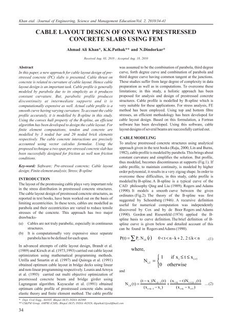
Cable layout design of one way prestressed concrete slabs using ...

Journal of Engineering, Science and Management EducationIn above equations, P are the n+1 defining polygon vertices,i'sk is the order of the B spline and N (t) is called the weighingi,kfunction. x is the additional knot vector which is used for B-spline curve to account for the inherent added flexibility. Aknot vector is simply a series of real integers x such thatix x for all x . They are used to indicate the parameter ti i+1 iused to generate a B-spline The curve generally follows theshape of the defining polygon and the curve is transformed bytransforming the defining polygonal vertices. The order of theresulting curve can be changed without changing the numberof defining polygon vertices. In Figure : 4 cable reactionconsidering parabolic and B-spline are shown. It can beobserved that B-spline represents the realistic profile. Whena B-spline curve is used, the geometrical regularity isautomatically taken into account. Braibant and Fleury(1984), Pourazady et al. (1996) and Ghoddosian(1998) haveused this curve in shape optimization problems and cablegeometry is being modeled as B-spline in this studyFINITE ELEMENT MODELINGFor realistic analysis of PC structures advanced computingtechniques such as finite element method has beenextensively employed in literature. Linear finite elementanalysis (FEA) of pre-stressed concrete structures hasbeen reported by Pandey et al. (1997),Buragohian et al(1993,1997),Pathak et al.(2004. Non linear analysis of thesame are reported by Povoas et al. (1989), Kang et al. (1990),Roca et al. (1993), Greunen et al. (1983), Figueiras et al.(1994), Vanzyl et al. (1979) and Elwi et al. (1987). Jirousek etal. (1979) and Buragohain et al. (1993,1997) have consideredcable as parabolic and cubic curve in shell and semiloofshell elements, whereas Pandey et al. (1997) considered thecable as parabola in 20 node brick element. Pathak et al.(2004) considered the cable as cubic spline curve in nine nodeLagrangean element. Saleem Akhtar et al. (2008) modelledcable as B-spline for two dimensional finite element analysis.In this study, cable is modeled by three noded bar element andconcrete by 20 noded brick element (Zienkiewicz and Tayler1991). In Fig.4, a 3 node curved bar element is shown which isembedded in three dimensional 20 node concrete element.Cable will exert normal and tangential forces on the concreteas shown in Fig.5.The shape functions of a 3 node curved bar elements along ñaxis are given by-( ρ−1)ρN c 1=2Nc2 = (1 − ρ)(1 + ρ)...................(3)The global coordinates on the curved bar element is given by⎧x⎫⎧x⎫3 3⎪ ⎪ ⎪ ⎪X = ⎨y⎬= ∑⎨y⎬N = ∑X N⎪z⎪⎪z⎪⎩ ⎭ ⎩ ⎭The tangent vector and normal vector along ñ axis for thecable is given by=Where, a is the dot product.ci i cii= 1 i=1dN3ciT = ∑ Xii=1 dρT1⎛ 2⎞⎜ d X a dX ⎟⎜ −2 ⎟dρ T dρ⎝⎠N22a =dρ2dX d X.2dρThe unit tangent and normal vector can be given byTt =| T |Nn =| N |The curvature at any point on the cable is expressed byKdX×dρdρ2d X2=23/2⎧ ⎫⎪ dX⎨⎪ d ρ⎩Now radius of curvature can be calculated by :1R =K(4)(5)(6)(7)(8)(9)(10)NORMAL AND TANGENTIAL FORCESThe cable exerts tangential and normal forces on concrete dueto intaraction between contacting surfaces and curvature ofthe cable as shown in Fig.5.Tangential and normal forces can be expressed as:⎪⎬⎪⎭N c 3( ρ + 1) ρ=2dTnPt=dX=1TdTndρ(11)35

Journal of Engineering, Science and Management EducationTnPn=RNow the resultant force can be computed by(12)In above equation inverse matrix is the jacobian matrix. (x i+1,y i+1, z i+1) and (x i, y i, z i) are the known and computed values ofthe global co-ordinates. Starting values of î, ç, æ areconsidered as 0, 0, 0. The prescribed tolerance is 0.01.P = P tt+P n(13)Where T is the tension in the cable and T is the tangent vector.nUsing the principle of virtual work, these loads can betransferred to the nodes of brick elements. The equivalentnodal force vector for brick element is given by-1T{ PL} = ∫ [ N] P | T | dρ (14)−1Cable reaction acts as concentrated loads on the concrete atthe ends, where cable is anchoraged. The anchorage end pointforces can be calculated by-(15)Where, T is the cable tension at the end points and [N] is theendshape functions of 20 node brick elements. Local coordinatesare required for known global coordinates for calculation ofanchorage end point forces .This is described in next section.Now total load vector due to interaction of concrete and cableis obtained by-(16)This nodal load vector is applied on the three dimensionalfinite element model along with live and dead load vectors toinclude pre-stressing effects.LOCAL COORDINATES COMPUTATIONEvaluation of local co-ordinate corresponding to knownglobal coordinates is an inverse nonlinear problem which canbe solved by Newton-Raphson method. The computation iscarried out iteratively till the difference of two consecutivevalues becomes less than the prescribed tolerance. Let (x,y,z)is the global coordinate and ( î,ç,æ ) be the correspondinglocal co-ordinate. Numerical computations of local coordinatescan be obtained using following iterativerelationship-⎧ξ⎫⎪ ⎪⎨η⎬⎪ ⎪⎩ς⎭⎧ξ⎫⎪ ⎪= ⎨η⎬⎪ ⎪⎩ς⎭n{}{ P } = [ N] T TA{ }end{ P} = { P} + { P}T L A⎛ ∂x⎜⎜ ∂ξ⎜ ∂y+⎜ ∂ξ⎜∂z⎜⎝ ∂ξ∂x∂η∂y∂η∂z∂η∂x⎞⎟∂ς⎟∂y⎟∂ς⎟∂z⎟⎟∂ς⎠−1⎧ x⎪⎨ y⎪⎩ zi+1i+1− xi⎫⎪− yi ⎬− z ⎪⎭i+ 1ii+1 i....... (17)CABLE LAYOUT DESIGNAn algorithm has been developed to find the cable layout sothat stresses in the structural element be below the limitingtensile stress. A check on the compressive stresses will bemade in order to avoid crushing of the concrete. Based onstress results obtained from finite element analysis, cableprofile is changed in iterative manner. In the followingsections, these are described in detail.Criterion for Layout DesignOne of the main objective of the prestressed concrete designis to get rid of the tensile stresses from the concreteproduced due to different loading conditions. In Fig.6 aprestressed concrete structure is shown. It is assumed thattop fiber at sections 1 and 3 are in tension and bottomfiber at section 2 is in tension. The shape of the cable toeliminate the tension should be as shown in the samefigure. The shape of the cable can be represented by a B-spline. By varying the ordinates of the B-spline, cableshape is changed to get the desired profile. It is alsoimportant to know that this would be very difficult if notimpossible with any other curve.Algorithm for Layout DesignIn Fig.7, a concrete beam with typical loading is selected forcable layout design. Assume the cable to be straightbetween anchorage ends and initial prestressing force beP. Now finite element analysis of the beam is carried outfor external loads and initial prestressing force P actingat the ends. Let sections 1,2,3,4 and 5 be such that bottomfiber of 1, 3 and 5 are in tension and top fiber of 2 and4 are in tension. Assume top and bottom stresses at thesesections beitandib, where i varies from 1 to 5.Since stresses at bottom fiber at 1,3 and 5 are in tension,the cable should be concave there, whereas at 2 and 4 itshould be convex. The ordinates of B-spline will movedownward at 1,3 and 5 and will move upward at 2 and4. Let the initial y-coordinates of these points be y 1,y ,y ,y and y . Depending upon top and bottom fiber2 3 4 5stresses at a point, following four cases may be framed:(a). Top fiber is in tension and bottom fiber is incompression.(b). Bottom fiber is in tension and top fiber is incompression.(c). Both fibers are in tension.(d). Both fibers are in compression.36

Journal of Engineering, Science and Management Education(a) Top fiber is in tension and bottom fiber is incompressionLetitandibbe top and bottom stresses, then a ratio R isdefined asR =σitσit+ abs( σ ib)(18)where abs is the absolute value. New y-coordinates of theB-spline ordinates are calculated as-i+1= (1 + R y i(19)here y represents the y-coordinate of the previousiiteration.(b) Bottom fiber is in tension and top fiber is incompressionLike previous case the stress ratio is defined in thefollowing way-R =σy )ibσ+ absib( σ it(20)once again abs represents the absolute value. New y-coordinates of the B-spline ordinates are calculated as:y )(21)A check on the compressive stresses at the top fiber will bemade for it to not cross the limiting value.(c) Both Fibers are in TensionIf top and bottom both fibers are in tension, then eitherthe cable force should be increased or the section should beredesigned.(d) Both Fibers are in CompressionCheck the compressive stresses at the top and bottom fibersfor them to not cross the limiting value. If they are below,cable profile is not altered at that section otherwiseredesign the section.These steps are repeated till the cable profile for limitingtensile stresses is obtained. Based on this procedure,ordinate movements of B-spline are shown in Fig.7.The flowchart of the proposed algorithm is shown in Fig.8.Using this a FORTRAN software PRECLAD3D has beendeveloped. The software has been successfully run on aPentium IV processor using Microsoft FORTRAN Powerstation compiler.)i+1= (1 − R y i\7 NUMERICAL EXAMPLESA two span, one way prestressed concrete slab of8000x2000x400 mm is designed using PRECLAD3Dsoftware for friction and non friction conditions. The slab isdiscretised into 50 twenty node brick elements and 428nodes. The loading conditions and FE model are shown inFig.9. Two line loads are applied in each span of the slab.Corresponding nodal point loads in terms of A, B, C are 20, 40and 10 KN respectively. P is the prestressing force. Followingmaterial properties are used for the design purposes-4 2(a). Young's modulus (concrete) = 2x10 N/mm2(b). Compressive strength of concrete = 40 N/mm(c). Poisson's ratio = 0.15-5(d). Wobble coeffient = 1x10(e) Coefficient of friction = 0.202(f). Tensile strength of concrete = 0.25 N/mm .3(g). Density of concrete = 2500 Kg/mThe limiting tensile stress is considered as 0.25 MPa. Becauseof symmetry cables 1,2 and and 4, 5 will have same profile.In Table 1, top and bottom bending stresses at differentsections for without friction condition are given. The intialthprestressing force is 480 KN. It can be observed that in 12iterations, tensile stresses are below the limiting value. Thefinal prestressing force is 494 KN. Cable eccentricities interms of polygon and B-spline ordinates are given in Table 2.In Table 3, top and bottom bending stresses at differentsections for friction condition are given. The intialthprestressing force is 560 KN. It can be observed that in 7iterations, tensile stresses are below the limiting value. Thefinal prestressingn force is 588 KN. Cable eccentricities interms of polygon and B-spline ordinates are given in Table 4.The percentage increase in the final load with respect to that ofnon friction case is 19% which is required to overcomefriction.CONCLUSIONSIn this paper a new technique for cable layout design ofprestressed concrete slabs is presented. The pre-stressingcables are modelled as B-spline curve. Friction loss of theprestressing force is also accounted. The cable segment in thefinite element is modelled by three node bar element. Thisapproach is coded in a 3D FE software using which twoprestressed concrete slabs have been successfully designed. Itis hoped that the proposed approach will prove to be aneffective tool of the design engineers in realistic design of PCslabs.37

Journal of Engineering, Science and Management EducationItNo1.2.3.4.5.6.7.8.9.10.11.12.Load(KN)480480480480480480480490490490493494Table 1: Bending stresses (MPa) (without friction)Section Cable 1 Cable 2 Cable 3Top Bottom Top Bottom Top Bottom1-1 -6.366 0.292 -6.348 0.233 -6.336 0.2132-2 0.350 -6.661 0.486 -6.452 0.501 -6.4463-3 -6.375 -0.306 -6.350 0.248 -6.338 0.2281-1 -6.271 0.198 -6.254 0.141 -6.243 0.1212-2 0.277 -6.586 0.412 -6.378 0.427 -6.3723-3 -6.271 0.203 -6.247 0.146 6.236 0.1271-1 -6.191 0.118 -6.175 0.062 -6.164 0.0432-2 0.247 -6.556 0.381 -6.349 0.397 -6.3433-3 -6.239 0.172 -6.215 0.114 -6.204 0.0951-1 -6.154 0.083 -6.140 0.027 -6.129 0.0082-2 0.220 -6.529 0.354 -6.323 0.370 -6.3173-3 -6.171 0.105 -6.148 0.048 -6.137 0.0291-1 -6.124 0.053 -6.110 0.002 -6.099 -0.0212-2 0.208 -6.518 0.343 -6.312 0.359 -6.3083-3 -6.128 0.062 -6.105 0.006 -6.095 -0.0121-1 -6.098 -0.027 -6.084 -0.027 -6.073 -0.0462-2 0.205 -6.516 0.341 -6.312 0.358 -6.3083-3 -6.098 0.033 -6.076 -0.022 -6.065 -0.0421-1 -6.074 0.004 -6.061 -0.050 -6.050 -0.0692-2 0.212 -6.524 0.348 -6.322 0.366 -6.3183-3 -6.082 0.016 -6.059 -0.039 -6.048 -0.0581-1 -6.116 -0.080 -6.103 -0.134 -6.092 -0.1532-2 0.133 -6.573 0.270 -6.367 0.288 -6.3633-3 -6.123 -0.067 -6.101 -0.123 -6.091 -0.1421-1 -6.098 -0.097 -6.085 --0.152 -6.074 -0.1712-2 0.137 -6.578 0.275 -6.373 0.293 -6.3703-3 -6.106 -0.084 -6.083 -0.140 -6.073 -0.1591-1 -6.140 -0.056 -6.127 -0.110 -6.116 -0.1292-2 0.126 -6.565 0.262 -6.357 0.279 -6.3523-3 -6.140 -0.050 -6.118 -0.106 -6.108 -0.1251-1 -6.152 -0.081 -6.139 -0.135 -6.129 -0.1542-2 0.102 -6.580 0.239 -6.370 0.256 -6.3663-3 -6.153 -0.075 -6.131 -0.131 -6.121 -0.1501-1 -6.157 -0.089 -6.144 -0.144 -6.133 -0.1632-2 0.094 -6.584 0.231 -6.375 0.248 -6.3703-3 -6.157 -0.083 -6.135 -0.139 -6.125 -0.158Table 2: Cable eccentricity (mm) at different sections (without friction)Cable No Cable1 Cable2 Cable3Distance from left end 0 1600 4000 6400 8000 0 1600 4000 6400 8000 0 1600 4000 6400 8000(mm)ItNoLoad(KN)Ordinate1. 480 Polygon 200 150 250 150 200 200 150 250 150 200 200 150 250 150 200B-spline 200 178.40 200 178.40 200 200 178.40 200 178.40 200 200 178.40 200 178.45 2002. 480 Polygon 200 143.42 262.48 148.12 200 200 144.68 267.51 144.36 200 200 145.12 268.03 144.79 200B-spline 200 176.59 202.87 176.41 200 200 178.24 206.01 178.05 200 200 178.6 206.49 178.41 2003. 480 Polygon 200 139.03 273.07 143.47 200 200 141.49 283.74 141.06 200 200 142.4 284.86 141.9 200B-spline 200 175.86 207.16 178.42 200 200 179.15 212.50 178.90 200 200 179.9 213.5 179.61 2004. 480 Polygon 200 136.42 282.98 139.62 200 200 140.08 299.80 138.52 200 200 141.41 301.63 139.75 200B-spline 200 175.99 210.50 177.84 200 200 181.10 219.55 180.20 200 200 182.23 221.10 181.28 2005. 480 Polygon 200 134.60 292.20 137.28 200 200 139.47 315.69 137.45 200 200 141.22 318.32 139.09 200B-spline 200 176.50 214.07 178.05 200 200 183.53 227.07 182.36 200 200 185.05 229.23 183.82 2006. 480 Polygon 200 133.44 301.23 135.90 200 200 139.47 331.96 137.31 200 200 141.22 335.46 139.09 200B-spline 200 177.38 217.95 178.8 200 200 186.38 235.17 185.14 200 200 188.06 237.80 186.84 2007. 480 Polygon 200 133.44 310.42 136.54 200 200 139.47 348.97 137.31 200 200 141.22 353.47 139.09 200B-spline 200 179.01 222.70 180.80 200 200 189.31 243.68 188.13 200 200 191.23 246.81 190.01 2008. 490 Polygon 200 133.44 310.42 136.54 200 200 139.47 348.97 137.31 200 200 141.22 353.47 139.09 200B-spline 200 179.01 222.70 180.80 200 200 189.31 243.68 188.13 200 200 191.23 246.81 190.01 2009. 490 Polygon 200 133.44 316.57 136.54 200 200 139.47 363.17 137.31 200 200 141.22 368.77 139.09 200B-spline 200 180.09 225.78 181.88 200 200 191.88 250.78 190.63 200 200 193.93 254.46 192.70 20010. 490 Polygon 200 133.44 301.23 135.90 200 200 139.47 331.96 137.31 200 200 141.22 335.46 139.09 200B-spline 200 177.38 217.95 178.8 200 200 186.38 235.17 185.14 200 200 188.06 237.8 186.84 20011. 493 Polygon 200 133.44 301.23 135.90 200 200 139.47 331.96 137.31 200 200 141.22 335.46 139.09 200B-spline 200 177.38 217.95 178.80 200 200 186.38 235.17 185.14 200 200 188.06 237.80 186.84 20012. 494 Polygon 200 133.44 301.23 135.90 200 200 139.47 331.96 137.31 200 200 141.22 335.46 139.09 200B-spline 200 177.38 217.95 178.80 200 200 186.38 235.17 185.14 200 200 188.06 237.80 186.84 20038

Journal of Engineering, Science and Management EducationItNo1.2.3.4.5.6.7.Load(KN)560560560560570580588Table 3: Bending stresses (MPa) (with friction)Section Cable 1 Cable 2 Cable 3Top Bottom Top Bottom Top Bottom1-1 -6.938 0.536 -6.917 0.474 -6.902 0.4532-2 0.361 -6.991 0.504 -6.773 0.521 -6.7673-3 -6.383 0.095 -6.360 0.048 -6.349 -0.0681-1 -6.705 0.330 -6.686 0.270 -6.673 0.2502-2 0.307 -6.991 0.450 -6.694 0.467 -6.6883-3 -6.398 0.050 -6.375 -0.007 -6.364 -0.0261-1 -6.561 0.206 -6.544 0.148 -6.531 0.1282-2 0.283 -6.866 0.425 -6.651 0.442 -6.6463-3 -6.396 0.068 -6.373 0.010 -6.362 -0.0091-1 -6.473 0.136 -6.457 0.079 -6.445 0.0592-2 0.274 -6.840 0.416 -6.627 0.434 -6.6223-3 -6.370 0.060 -6.347 0.003 -6.337 -0.0161-1 -6.516 0.066 -6.500 0.009 -6.488 -0.0092-2 0.207 -6.888 0.350 -6.671 0.368 -6.6663-3 -6.411 -0.010 -6.389 -0.067 -6.378 -0.0871-1 -6.558 -0.063 -6.544 -0.059 -6.532 -0.0792-2 0.140 -6.935 0.285 -6.715 0.302 -6.7093-3 -6.452 -0.081 -6.430 -0.138 -6.419 -0.1581-1 -6.592 -0.059 -6.578 -0.115 -6.566 -0.1352-2 0.086 -6.973 0.232 -6.750 0.250 -6.7443-3 -6.484 -0.138 -6.463 -0.194 -6.453 -0.214Table 4: Cable eccentricity(mm) at different section-with frictionCable No Cable 1 Cable 2 Cable 3Distance from left end 0 1600 4000 6400 8000 0 1600 4000 6400 8000 0 1600 4000 6400 8000(mm)ItNoLoad(KN)Ordinate1. 560 Polygon 200 150 250 150 200 200 150 250 150 200 200 150 250 150 200B-spline 200 178.40 200 178.40 200 200 178.40 200 178.40 200 200 178.40 200 178.45 2002. 560 Polygon 200 139.42 262.27 147.80 200 200 140.38 267.31 150 200 200 140.76 267.87 150 200B-spline 200 174.26 202.94 179.08 200 200 175.71 206.25 181.29 200 200 176.07 206.62 181.39 2003. 560 Polygon 200 132.88 273.30 146.65 200 200 134.93 284.14 150 200 200 135.67 285.35 150 200B-spline 200 172.31 206.53 180.24 200 200 175.48 213.30 184.16 200 200 176.13 214.09 184.39 2004. 560 Polygon 200 128.83 284.12 145.10 200 200 131.94 301.20 149.76 200 200 133.06 303.14 150 200B-spline 200 171.79 210.54 181.16 200 200 176.71 221.02 186.98 200 200 177.72 222.33 187.48 2005. 570 Polygon 200 128.83 284.12 145.10 200 200 131.94 301.20 149.76 200 200 133.06 303.14 150 200B-spline 200 171.79 210.54 181.16 200 200 176.71 221.02 186.98 200 200 172.72 222.33 187.48 2006. 580 Polygon 200 128.83 284.12 145.10 200 200 131.94 301.20 149.76 200 200 133.06 303.14 150 200B-spline 200 171.79 210.54 181.16 200 200 176.71 221.02 186.98 200 200 177.72 222.33 187.48 2007. 588 Polygon 200 128.83 284.12 145.10 200 200 131.94 301.20 149.76 200 200 133.06 303.14 150 200B-spline 200 171.79 210.54 181.16 200 200 176.71 221.02 186.98 200 200 177.72 222.33 187.48 200ParabolicActualFig. 1 : Actual Cable & Parabolic ProfileFig. 2 : B-Spline Profile39

Journal of Engineering, Science and Management EducationFig. 3a : Parabolic ProfileFig. 6 : Required Cable ProfileFig. 3b : B-Spline ProfileFig. 7 : Variation of Cable ProfileStartSelection of slab loading, CableProfileChange the cableprofileNoIf stressesareincreasingYesIncrease the loadsNoFinite Element modelling,Boundary conditionsFinite Element analysis, Studyof bending stressesAre the stressesbelow limitingvalue?YesCable Layout completedStopFig. 4 : Brick Element with Curved Bar ElementFig. 8 : Flowchart for Cable Layout DesignFig. 8: Flow chart for cable layout designFig. 5 : Forces on Concrete Due to Cable Tension.Fig. 9 : Oneway Prestressed Concrete Slab.40

Journal of Engineering, Science and Management EducationREFERENCES1. A.M. Brandt. “Foundations of Optimum Design in CivilEngineering,” Nijhoff Publishers, 1989.2. V. Braibant , C. Fleury, P. Beckers. “Shape optimaldesign: An approach matching CAD and optimizationconcept,” Report SA-109, Aerospace Laboratory ofUniversity of Liege, Belgium, 1983.3. D.N. Buragohian , A. Mukherjee. “PARCS –A prestressedand reinforced concrete shell element forthanalysis of containment structures,” Transac. of 12SmiRT Int. Conf, Vol. B, Stuttgart, Germany, 1993.4. D.N. Buragohian, U.R. Siddhyae. “Finite elementanalysis of pre stressed concrete box girder bridges,” J.Struc. Engg. Div., 24(3), 135-141, 1997.5. A. Elwi , T. Hrudey. “Finite element model for curvedcable embedded reinforcement,” J. Engg. Mech.ASCE, 115 (4), 740-754, 1989.6. J.A. Figueiras , R.H.C.F. Povoas. “Modeling of prestressingin non -linear analysis of concrete structures,”Comput. & Struc., 53(1), 173-187,1994.7. A. Ghoddosian. “Improved Zero Order Techniques forStructural Shape Optimization Using FEM,” PhDDissertation, Applied Mechanics Dept. IIT Delhi, 1998.8. W.J. Gordon, R.F. Riesenfeld . “Computer AidedGeometric Design,” Academic Press, London, 1974.9. J.V. Greunen, A.C. Scordelis. “Nonlinear analysis ofpre-stressed concrete slabs,” J. Struct. Engg. Div.,ASCE, 109 (7), 1742-1760, 1983.10. J. Jirousek , A. Bouberguig , A. Saygun . “A macroelement analysis of pre-stressed curved box girderbridges” Comput. & Struc., 10, 467-482, 1979.11. Y.J. Kang , A. C. Scordelis. “Non-linear analysis of prestressedconcrete frames,” J. Struct. Engg. Div., ASCE,106(2), 445-462, 1990.12. U. Kirsch. “Optimized prestressing by linearprogramming,” Int. J. Num. Meth. Engg., 7, 125-136,1973.13. U. Kirsch. “Structural Optimization, Springer-Verlog,Berlin, 1993.14. A. Kuyucular. “Prestressing optimization of concreteslabs,” J. Struct. Engg. Div., ASCE, 117, 235-254,1991.15. Z. Lounis , M.Z. Cohn. “Multi objective optimizationof prestressed concrete structures,” J. Struct. Engg.Div., ASCE, 119, 794-808, 1993.16. T.Y Lin, N.H. Burns. “Design of pre-stressedconcrete structures,” Third Edition, John Wiley andSons. Inc., New York, 1982.17. A.K. Pandey, R. Kumar, D.N. Trikha. “Finite elementanalysis of pre-stressed concrete containmentstructures,” Proceedings of first internationalconference on computer aided analysis and design,Hyderabad, India, 373-379, 1997.18. K.K. Pathak, D. K. Sehgal. “Analysis of pre-stressconcrete beams using different cable models,” J. Bridgeand Struc. Engg., 33, 2004.19. M. Pourazady , Z. Fu . “An integrated approach tostructural shape optimization,” Comput. and Struct.,60, 279-289,1996.20. R.H.C.F Povoas, J.A. Figueiras. “Non linear analysis ofcurved pre-stressed girder bridges,”. Proceedings ofsecond international conference on computer aidedanalysis and design, Austria, 1989.21. S.B. Qing, D.Y. Liu . “Computational geometry- Curveand Surface Modeling,” Academic Press, London,1989.22. A.S. Quiroga,n M.A.U Arroya. “Optimization ofprestressed concrete bridge decks,” Comput. andStruct., 41, 553-559, 1991.23. N.K. Raju. “Pre-stressed Concrete,” Third Edition,New Delhi, Tata Mc -Graw Hill, 1995.24. P. Roca, A.R. Mari. “Numerical treatment of prestressingtendons in the non- linear analysis of prestressedconcrete structures,” Comput. and Struc., 46(950), 905-916 , 1993.25. D.F. Rogers, J.A. Adams . “Mathematical Element forcomputer Graphics,” Second Edition, McGraw-Hill,New York,1990.26. S. Akhtar, K.K. Pathak, S.S. Bhaduria. “Finite elementanalysis of pre-stress concrete beams consideringrealistic cable profile,” Int. J. Appl. Engg., Res.,, 3(1) ,2008.27. I.J. Schoenberg. “Contribution to the problem ofapproximation of equidistant data by analyticfunctions,” Quarterly of Appl. Math., 4 ,45-99, 1946.28. M.A. Utrilla, A. Smartin . “Optimized design of theprestress in continuous bridge decks,” Comput. andStruct., 64, 719-728,1997.29. S.F. Vanzyl, A.C. Scordelis. “Analysis of curved prestressedsegmental bridges,” J. Struc. Engg., ASCE,105, 2399 -2411,1979.30. O.C. Zienkiewicz, R.L. Taylor. The Finite ElementMethod Vol. 1&2, Fourth Edition: McGraw -HillLondon, 1991.41