Slim: Directly Mining Descriptive Patterns - Universiteit Antwerpen

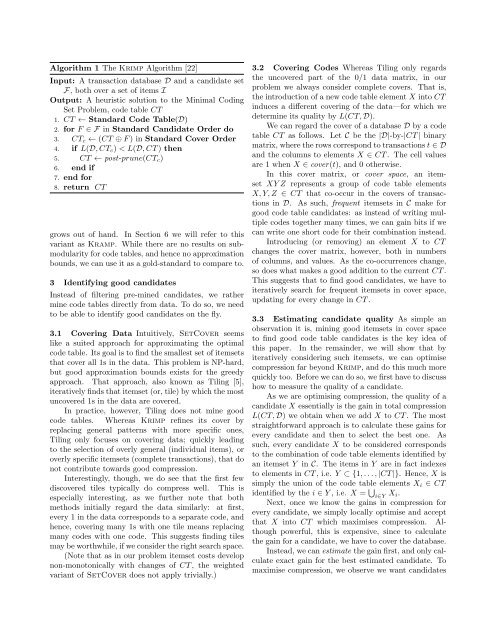
Algorithm 1 The Krimp Algorithm [22]Input: A transaction database D and a candidate setF, both over a set of items IOutput: A heuristic solution to the Minimal CodingSet Problem, code table CT1. CT ← Standard Code Table(D)2. for F ∈ F in Standard Candidate Order do3. CT c ← (CT ⊕ F ) in Standard Cover Order4. if L(D, CT c ) < L(D, CT ) then5. CT ← post-prune(CT c )6. end if7. end for8. return CTgrows out of hand. In Section 6 we will refer to thisvariant as Kramp. While there are no results on submodularityfor code tables, and hence no approximationbounds, we can use it as a gold-standard to compare to.3 Identifying good candidatesInstead of filtering pre-mined candidates, we rathermine code tables directly from data. To do so, we needto be able to identify good candidates on the fly.3.1 Covering Data Intuitively, SetCover seemslike a suited approach for approximating the optimalcode table. Its goal is to find the smallest set of itemsetsthat cover all 1s in the data. This problem is NP-hard,but good approximation bounds exists for the greedyapproach. That approach, also known as Tiling [5],iteratively finds that itemset (or, tile) by which the mostuncovered 1s in the data are covered.In practice, however, Tiling does not mine goodcode tables. Whereas Krimp refines its cover byreplacing general patterns with more specific ones,Tiling only focuses on covering data; quickly leadingto the selection of overly general (individual items), oroverly specific itemsets (complete transactions), that donot contribute towards good compression.Interestingly, though, we do see that the first fewdiscovered tiles typically do compress well. This isespecially interesting, as we further note that bothmethods initially regard the data similarly: at first,every 1 in the data corresponds to a separate code, andhence, covering many 1s with one tile means replacingmany codes with one code. This suggests finding tilesmay be worthwhile, if we consider the right search space.(Note that as in our problem itemset costs developnon-monotonically with changes of CT , the weightedvariant of SetCover does not apply trivially.)3.2 Covering Codes Whereas Tiling only regardsthe uncovered part of the 0/1 data matrix, in ourproblem we always consider complete covers. That is,the introduction of a new code table element X into CTinduces a different covering of the data—for which wedetermine its quality by L(CT, D).We can regard the cover of a database D by a codetable CT as follows. Let C be the |D|-by-|CT | binarymatrix, where the rows correspond to transactions t ∈ Dand the columns to elements X ∈ CT . The cell valuesare 1 when X ∈ cover(t), and 0 otherwise.In this cover matrix, or cover space, an itemsetXY Z represents a group of code table elementsX, Y, Z ∈ CT that co-occur in the covers of transactionsin D. As such, frequent itemsets in C make forgood code table candidates: as instead of writing multiplecodes together many times, we can gain bits if wecan write one short code for their combination instead.Introducing (or removing) an element X to CTchanges the cover matrix, however, both in numbersof columns, and values. As the co-occurrences change,so does what makes a good addition to the current CT .This suggests that to find good candidates, we have toiteratively search for frequent itemsets in cover space,updating for every change in CT .3.3 Estimating candidate quality As simple anobservation it is, mining good itemsets in cover spaceto find good code table candidates is the key idea ofthis paper. In the remainder, we will show that byiteratively considering such itemsets, we can optimisecompression far beyond Krimp, and do this much morequickly too. Before we can do so, we first have to discusshow to measure the quality of a candidate.As we are optimising compression, the quality of acandidate X essentially is the gain in total compressionL(CT, D) we obtain when we add X to CT . The moststraightforward approach is to calculate these gains forevery candidate and then to select the best one. Assuch, every candidate X to be considered correspondsto the combination of code table elements identified byan itemset Y in C. The items in Y are in fact indexesto elements in CT , i.e. Y ⊂ {1, . . . , |CT |}. Hence, X issimply the union of the code table elements X i ∈ CTidentified by the i ∈ Y , i.e. X = ⋃ i∈Y X i.Next, once we know the gains in compression forevery candidate, we simply locally optimise and acceptthat X into CT which maximises compression. Althoughpowerful, this is expensive, since to calculatethe gain for a candidate, we have to cover the database.Instead, we can estimate the gain first, and only calculateexact gain for the best estimated candidate. Tomaximise compression, we observe we want candidates