Slim: Directly Mining Descriptive Patterns - Universiteit Antwerpen

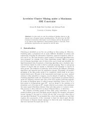
Slim: Directly Mining Descriptive PatternsKoen SmetsJilles VreekenAdvanced Database Research and ModellingUniversiteit Antwerpen{koen.smets,jilles.vreeken}@ua.ac.beAbstractMining small, useful, and high-quality sets of patternshas recently become an important topic in data mining.The standard approach is to first mine many candidates,and then to select a good subset. However, the patternexplosion generates such enormous amounts of candidatesthat by post-processing it is virtually impossibleto analyse dense or large databases in any detail.We introduce Slim, an any-time algorithm formining high-quality sets of itemsets directly from data.We use MDL to identify the best set of itemsets asthat set that describes the data best. To approximatethis optimum, we iteratively use the current solutionto determine what itemset would provide most gain—estimating quality using an accurate heuristic. Withoutrequiring a pre-mined candidate collection, Slim isparameter-free in both theory and practice.Experiments show we mine high-quality patternsets; while evaluating orders-of-magnitude fewer candidatesthan our closest competitor, Krimp, we obtainmuch better compression ratios—closely approximatingthe locally-optimal strategy. Classification experimentsindependently verify we characterise data very well.1 IntroductionPattern mining is one of the central topics in datamining, and is focused on discovering interesting localstructure in data. Starting from frequent sets andassociation rules [1], one of the key goals in patternmining has been completeness: discovering all patternsthat satisfy certain conditions. In a way, this is a usefulgoal, as we know that all returned patterns meet therequirements—and as such, are potentially interesting.Completeness, however, also has its drawbacks.Typically, there exist extremely many patterns fulfillingthe constraints, many of which convey the same information.Mining all patterns hence leads to prohibitivelylarge and strongly redundant results, which are in turndifficult to use or interpret. To address this, researchershave recently instead focused on discovering small anduseful, high-quality sets of patterns [12, 8, 22].We identify the best set of patterns as those patternsthat together describe the data best. That is, bythe Minimum Description Length (MDL) principle [6],we are after that set of patterns that provides the optimallossless compression of the data. By definition, thisset has many desirable properties: it is non-redundant,not overly simple, nor complex for the data—as otherwise,bits could have been saved. The main question is,how do we mine this optimal result?In this paper, we present Slim, an efficient heuristicfor directly mining high-quality data descriptions ontransaction data. Slim is a fast, one-phase, any-timealternative to Krimp [17]. Besides obtaining bettercompression, it can handle large and dense datasets,and is parameter-free in both theory and practice.The MDL approach to pattern mining was pioneeredby Siebes et al. [17, 22], who gave the Krimpalgorithm to approximate the optimal set of itemsets,or, code table. Subsequent research showed these setsof patterns to be very useful. Besides characterising thedistribution of the data very well, they have been shownto provide high performance in a wide range of tasks, includingdifference measurement [21], clustering [9], andoutlier detection [18].Like many pattern set mining approaches [7, 2, 16],Krimp follows a straightforward two-phase approachto mining code tables. First, it mines a collection offrequent itemsets. Second, it considers these candidatesin a static order, accepting a pattern if it improvescompression. This simplicity has some drawbacks.First of all, mining candidates is expensive. Asmore candidates correspond to a larger search space,lower support thresholds correspond to better finalresults. Often, however, it is difficult to keep the numberof candidates feasible—for large and dense databasesespecially, a small drop of the threshold can lead toan enormous increase in patterns. Moreover, as mostcandidates will be rejected, this step is quite wasteful.Second, by considering candidates only once, and ina fixed order, Krimp sometimes rejects candidates that

it could have used later on. A more powerful strategywould be to iteratively select the best addition out of allcandidates—which naively, however, quickly becomesinfeasible for larger databases or candidate collections.With Slim, we address these issues, and give anefficient any-time algorithm for mining descriptive patternsets directly from data. We greedily construct patternsets in a bottom-up fashion, iteratively joining cooccurringpatterns such that compression is maximised.To reduce computation and database scans, it employsa simple yet accurate heuristic to estimate the gain orcost of introducing a candidate. Importantly, Slim isparameter-free in both theory and practice.Experiments show we discover high-quality patternsets. The Slim code tables attain very high compressionratios; in particular on large and dense datasets,we obtain tens of percentages better compression thanKrimp, while considering orders-of-magnitude fewercandidates. Classification experiments show high accuracy,verifying that we characterise the data well. Convergenceplots show Slim closely approximates the powerfulgreedy approach of selecting the best candidate outof all candidates; all while being much more efficient.The remainder of this paper is organised as follows.First, we cover the preliminaries in Section 2 includingnotation, and short introductions to, resp. MDL, codetables, and Krimp. Next, in Section 3 we discusshow to mine and identify good candidate patterns. InSection 4 we introduce the Slim algorithm for mininghigh quality code tables directly from data. Section 5discusses related work, and we experimentally evaluateour method in Section 6. Finally, we round up withdiscussion in Section 7 and conclude in Section 8.2 PreliminariesIn this Section we give the notation used throughoutthe paper, and provide an introduction to MDL, codetables and the Krimp algorithm.2.1 Notation In this paper we consider transactiondatabases. Let I be a set of items, e.g. the productsfor sale in a shop. A transaction t ∈ P(I) is a set ofitems that, e.g. represent the items a customer bought.A database D over I is then a bag of transactions, e.g.the different sale transactions on a given day. We saythat a transaction t ∈ D supports an itemset X ⊆ I,iff X ⊆ t. The support of X in D is the number oftransactions in the database where X occurs.Note that any binary or categorical dataset can betrivially converted into a transaction database.Throughout this paper all logarithms are to base 2,and by convention we use 0 log 0 = 0.2.2 MDL, a brief introduction The MinimumDescription Length principle (MDL) [6], like its closecousin MML (Minimum Message Length) [23], is apractical version of Kolmogorov Complexity [10]. Allthree embrace the slogan Induction by Compression.For MDL, this can be roughly described as follows.Given a set of models M, the best model M ∈ Mis the one that minimisesL(M) + L(D | M) ,in which L(M) is the length in bits of the descriptionof M, and L(D | M) is the length of the description ofthe data when encoded with model M.This is called two-part MDL, or crude MDL—asopposed to refined MDL, where model and data areencoded together [6]. We use two-part MDL becausewe are specifically interested in the model: the patternsthat give the best description. Further, although refinedMDL has stronger theoretical foundations, it cannot becomputed except for some special cases.To use MDL, we have to define what our models Mare, how a M ∈ M describes a database, and how weencode these in bits. Note, that in MDL we are onlyconcerned with code lengths, not actual code words.2.3 Code tables As our itemset-based models weuse code tables [17, 22]. A code table is a simpledictionary: a two-column table with itemsets on theleft-hand side, and corresponding codes on its righthandside. The itemsets in the code table are orderedfirst descending on cardinality, second descending onsupport, and third lexicographically. We refer to thisas the Standard Cover Order.The actual codes on the right-hand side are of noimportance: their lengths are. To explain how theselengths are computed, the coding algorithm needs to beintroduced. A transaction t is encoded by searching forthe first itemset X in the code table for which X ⊆ t.The code for X becomes part of the encoding of t. Ift\X ≠ ∅, the algorithm continues to encode t\X. Sinceit is insisted that each code table contains at least allsingle items, this algorithm gives a unique encoding toeach (possible) transaction over I.The set of itemsets used to encode a transaction iscalled its cover. Note that the coding algorithm impliesthat a cover consists of non-overlapping itemsets. Thelength of the code of an itemset in a code table CTdepends on the database at hand; the more often a codeis used, the shorter it should be. To this end, we use anoptimal prefix code. To compute the code lengths, wehave to cover every transaction in the database.The usage of an itemset X ∈ CT is the number oftransactions t ∈ D which have X in their cover. The

elative usage of X ∈ CT is the probability that X isused in the encoding of an arbitrary t ∈ D. For optimalcompression of D, the higher Pr(X | D), the shorter itscode should be. In fact, from Information Theory [4],we have the Shannon entropy, which gives us the lengthof the optimal prefix code for X aswhereL(X | D) = − log Pr(X | D) ,Pr(X | D) =usage(X)∑usage(Y ) .Y ∈CTThe length of the encoding of transaction is now simplythe sum of the code lengths of the itemsets in its cover,∑L(t | CT ) = L(X | CT ) .X∈cover(t)The size of the encoded database is then the sum of thesizes of the encoded transactions,L(D | CT ) = ∑ t∈DL(t | CT ) .To find the optimal code table using MDL, we needto take both the compressed size of the database, andthe size of the code table into account. For the sizeof the code table, we only consider those itemsets thathave a non-zero usage. The size of the right-handside column is obvious; it is simply the sum of all thedifferent code lengths. For the size of the left-hand sidecolumn, note that the simplest valid code table consistsonly of the single items. This code table we refer toas the Standard Code Table, or ST . We encode theitemsets in the left-hand side column using the codes ofST . This allows us to decode up to the names of items.The encoded size of the code table is then given by∑L(CT | D) = L(X | ST ) + L(X | CT ) .X∈CTusage(X )≠0We define the optimal set of itemsets as the one whoseassociated code table minimises the total encoded sizeL(CT, D) = L(CT | D) + L(D | CT ) .More formally, we define the problem as follows.Minimal Coding Set Problem Let I be a setof items and let D be a dataset over I, cover a coveralgorithm, and F a collection of candidate patternsF ⊆ P(I). Find the smallest set of patterns S ⊆ Fsuch that for the corresponding code table CT the totalcompressed size, L(CT, D), is minimal.Using our cover algorithm only patterns occurringin D can be used in describing the data. As such, P(I)is a clear overestimate for what candidates the optimalCT can consist of. For reasons of efficiency, and withoutloss of generality, we can hence limit F to the collectionof all itemsets in D with a support of at least 1.Even for small F, however, the search space of allpossible code tables is rather large—and moreover, itdoes not exhibit structure nor monotonicity we can useto efficiently find the optimal code table [22]. Hence, weresort to heuristics.2.4 Introducing Krimp The Krimp algorithm wasintroduced by Siebes et al. [17, 22] as a straightforwardapproach for mining good approximations of the optimalcode table. Subsequent research showed these codetables to indeed be of high quality, and useful for a widerange of data mining tasks [21, 9, 22, 18].The pseudo-code of Krimp is given as Algorithm 1.It starts with the singleton code table (line 1), anda candidate collection F of frequent itemsets up toa given minsup. The candidates are ordered firstdescending on support, second descending on itemsetlength and third lexicographically. Each candidate F isconsidered in turn by inserting it in CT (3), denotedby CT ⊕ F , and calculating the new total compressedsize (4). It is only accepted if compression improves (4).If accepted, all elements X ∈ CT are reconsidered wrt.their contribution to compression (5).The minsup parameter is used to control the numberof candidates: the lower minsup, the more candidates,the larger the search space, and hence the betterthe approximation of the optimal code table. Asby MDL we are after the optimal compressor, minsupshould be set as low as practically feasible. Hence, technicallyminsup is not a parameter.In practice, however, keeping the number of itemsetsfeasible is difficult. Especially for dense or largedatabases, minute decreases in threshold give rise toenormous increases in patterns. Mining, sorting, andstoring these in large numbers takes non-trivial timeand effort, even before Krimp can begin selecting.Its robust empirical results aside, Krimp is a ratherrough greedy heuristic: it considers each candidate onlyonce, in a static order, raising the question how goodits approximations really are.A standard approach to hard optimisation problems,with provable approximation bounds in case ofsub-modular set functions [15], is to locally optimise thetarget function. For Krimp, local optimisation translatesto iteratively finding the F ∈ F that maximallyincreases compression. By considering F quadraticallyinstead of linearly, however, the running time quickly

Algorithm 1 The Krimp Algorithm [22]Input: A transaction database D and a candidate setF, both over a set of items IOutput: A heuristic solution to the Minimal CodingSet Problem, code table CT1. CT ← Standard Code Table(D)2. for F ∈ F in Standard Candidate Order do3. CT c ← (CT ⊕ F ) in Standard Cover Order4. if L(D, CT c ) < L(D, CT ) then5. CT ← post-prune(CT c )6. end if7. end for8. return CTgrows out of hand. In Section 6 we will refer to thisvariant as Kramp. While there are no results on submodularityfor code tables, and hence no approximationbounds, we can use it as a gold-standard to compare to.3 Identifying good candidatesInstead of filtering pre-mined candidates, we rathermine code tables directly from data. To do so, we needto be able to identify good candidates on the fly.3.1 Covering Data Intuitively, SetCover seemslike a suited approach for approximating the optimalcode table. Its goal is to find the smallest set of itemsetsthat cover all 1s in the data. This problem is NP-hard,but good approximation bounds exists for the greedyapproach. That approach, also known as Tiling [5],iteratively finds that itemset (or, tile) by which the mostuncovered 1s in the data are covered.In practice, however, Tiling does not mine goodcode tables. Whereas Krimp refines its cover byreplacing general patterns with more specific ones,Tiling only focuses on covering data; quickly leadingto the selection of overly general (individual items), oroverly specific itemsets (complete transactions), that donot contribute towards good compression.Interestingly, though, we do see that the first fewdiscovered tiles typically do compress well. This isespecially interesting, as we further note that bothmethods initially regard the data similarly: at first,every 1 in the data corresponds to a separate code, andhence, covering many 1s with one tile means replacingmany codes with one code. This suggests finding tilesmay be worthwhile, if we consider the right search space.(Note that as in our problem itemset costs developnon-monotonically with changes of CT , the weightedvariant of SetCover does not apply trivially.)3.2 Covering Codes Whereas Tiling only regardsthe uncovered part of the 0/1 data matrix, in ourproblem we always consider complete covers. That is,the introduction of a new code table element X into CTinduces a different covering of the data—for which wedetermine its quality by L(CT, D).We can regard the cover of a database D by a codetable CT as follows. Let C be the |D|-by-|CT | binarymatrix, where the rows correspond to transactions t ∈ Dand the columns to elements X ∈ CT . The cell valuesare 1 when X ∈ cover(t), and 0 otherwise.In this cover matrix, or cover space, an itemsetXY Z represents a group of code table elementsX, Y, Z ∈ CT that co-occur in the covers of transactionsin D. As such, frequent itemsets in C make forgood code table candidates: as instead of writing multiplecodes together many times, we can gain bits if wecan write one short code for their combination instead.Introducing (or removing) an element X to CTchanges the cover matrix, however, both in numbersof columns, and values. As the co-occurrences change,so does what makes a good addition to the current CT .This suggests that to find good candidates, we have toiteratively search for frequent itemsets in cover space,updating for every change in CT .3.3 Estimating candidate quality As simple anobservation it is, mining good itemsets in cover spaceto find good code table candidates is the key idea ofthis paper. In the remainder, we will show that byiteratively considering such itemsets, we can optimisecompression far beyond Krimp, and do this much morequickly too. Before we can do so, we first have to discusshow to measure the quality of a candidate.As we are optimising compression, the quality of acandidate X essentially is the gain in total compressionL(CT, D) we obtain when we add X to CT . The moststraightforward approach is to calculate these gains forevery candidate and then to select the best one. Assuch, every candidate X to be considered correspondsto the combination of code table elements identified byan itemset Y in C. The items in Y are in fact indexesto elements in CT , i.e. Y ⊂ {1, . . . , |CT |}. Hence, X issimply the union of the code table elements X i ∈ CTidentified by the i ∈ Y , i.e. X = ⋃ i∈Y X i.Next, once we know the gains in compression forevery candidate, we simply locally optimise and acceptthat X into CT which maximises compression. Althoughpowerful, this is expensive, since to calculatethe gain for a candidate, we have to cover the database.Instead, we can estimate the gain first, and only calculateexact gain for the best estimated candidate. Tomaximise compression, we observe we want candidates

1) with high usage (i.e. short codes), 2) replacing manycodes in C, while 3) not adding much complexity. Thefirst two of these properties are simply approximated byfinding frequent itemsets in C.However, we can say more on what itemsets wewant: highly frequent sets of only few items. Besidesthat these sets will likely compress well, they add littlecomplexity to CT . However, keeping in mind that byiteratively refining, if we consider too large itemsets in C,we strongly reduce our search space and are more likelyto end up in a local minimum. Moreover, calculatingthe gain in compression is most accurate for itemsetsof length 2. Hence, we restrict the cardinality of theitemsets we find in C to length 2. Note however, thatmore specific code table elements, i.e. large itemsets inD, can (and are) be constructed in only few iterations.Suppose X and Y are itemsets in CT . Let CT ′be the code table after adding the union of these twoitemsets, i.e. CT ′ = CT ⊕ X ∪ Y . We can estimate theusage of X ∪ Y in CT ′ as|usage(X) ∩ usage(Y )| ,where by usage(X) we slightly abuse notation to referto the tid list of transactions with X in their cover.Note this gives an upper bound to usage(X ∪Y ), whereequality only holds if X ∪ Y is considered for coveringright before when X or Y would be used. As code tableelements are ordered first on length, and the union oftwo non-equal itemsets produces a longer set, this isimplicitly enforced—making the bound quite tight.Although useful, as a gain estimate it is quite rough:it disregards the effects on L(CT | D) of adding X∪Y toCT , the increase of the code lengths of X and Y as theirusage decreases, as well as the scaling effect on all othercode lengths. We can improve our estimate by takingthese effects into account as follows, directly estimatingthe total compressed size for adding a candidate.Let ∆L be the difference in encoded size betweenCT and CT ′ ; or, in other words, the gain in bits forcandidate X ∪ Y . It is easy to see that ∆L for the totalencoded size consists of the difference in compressedsizes of the database, and the difference between theencoded sizes of the code tables,∆L(CT ⊕ X ∪ Y, D)= L(CT, D) − L(CT ⊕ X ∪ Y, D)= ∆L(D | CT ⊕ X ∪ Y ) + ∆L(CT ⊕ X ∪ Y | D) .For notational brevity, we use the lower case, x, ofan itemset X ∈ CT to indicate usage(X), i.e. x =usage(X). Then, let s be the sum of usages of CT , i.e.s = ∑ X∈CT x. Similarly, we use x′ and s ′ for CT ′ .Using this notation, we can write the difference in bitsbetween encoding D by either CT or CT ′ as follows,∆L(D | CT ⊕ X ∪ Y ) = s log s − s ′ log s ′ + xy ′ log xy ′− ∑(c log c − c ′ log c ′ ) ,C∈CTc≠c ′and the difference in the model complexity as∆L(CT ⊕ X ∪ Y | D) = log xy ′ − L(X ∪ Y | ST )+ |CT | log s − |CT ′ | log s ′ + ∑log c ′ − log c+ ∑C∈CTc ′ ≠cc=0C∈CTc ′ ≠cc ′ c≠0log c ′ − L(C | ST ) + ∑C∈CTc ′ ≠cc ′ =0L(C | ST ) − log c ,where xy ′ = usage(X ∪Y ) when using CT ′ . This meansthat we can express the gain in bits when adding X ∪ Yto CT only in terms of the usages of code table elementsfor which the usage changes between CT and CT ′ .In practice, however, it is hard to predict howusage(Z) for all Z ∈ CT will develop when a newelement X ∪ Y is inserted into CT . While we know theusages of Z ∈ CT ordered above X ∪ Y remain static, acascading effect may occur for those below it: in somet ∈ D, where some Z ∈ CT with Z ∩ (X ∪ Y ) ≠ ∅ waspreviously part of the cover of t, X ∪Y may now preventZ from being used; hence changing usage of Z, as well asthe usage of those Z ′ now used to cover Z \(X ∪Y ) of t,which in turn can block other previously used elements,etc.—potentially changing all usages.Although unpredictable, in practice the effect isnot often dramatic. Hence, for practical reasons, forestimating the gain we can assume only the usage ofX, Y , and X ∪ Y will change, using our above usageestimate for X ∪ Y . For calculating the estimated gainin total compressed size, we then simply use xy ′ =|usage(X) ∩ usage(Y )|, x ′ = x − xy ′ , y′ = y − xy ′ ands ′ = s−xy ′ . As such, we obtain a very easily calculable,and generally accurate estimate of ∆L for X ∪ Y .4 Directly Mining Descriptive PatternsWe can now combine the above results, and constructthe Slim algorithm for mining heuristic solutions to theMinimal Coding Set Problem directly from data. 1We give the pseudo-code as Algorithm 2. Slimstarts with the singleton-only code table ST (line 1).Every iteration (2) we consider all pairwise combinationsof X, Y ∈ CT as candidates in Gain Order, i.e.descending on ∆L(CT ⊕ (X ∪ Y ), D). Iteratively, weadd a candidate to CT in Standard Cover Order1 Slim is Dutch for smart, whereas Krimp means to shrink.

Algorithm 2 The Slim AlgorithmInput: A transaction database D over a set of items IOutput: A heuristic solution to the Minimal CodingSet Problem, code table CT1. CT ← Standard Code Table(D)2. for F ∈ {X ∪ Y : X, Y ∈ CT } in Gain Order do3. CT c ← (CT ⊕ F ) in Standard Cover Order4. if L(D, CT c ) < L(D, CT ) then5. CT ← post-prune(CT c )6. end if7. end for8. return CT(3), cover the data, and compute total encoded size (4).If compression improves, we accept the candidate, otherwisereject it. If accepted, we reconsider every elementin CT to whether it still contributes towards compression(5), and update the candidate list (2). We continueconsidering pairwise combinations of X, Y ∈ CT to refinethe current code table until no candidate decreasesthe total compressed size, after which we are done.Note that, if desired, extra constraints on individualcandidates (e.g. a minimum support, or length) can bechecked when constructing the candidate list, or beforeadding them to the code table at line 3.In practice, we do not need to materialise allcandidates on line 2. Instead, we traverse CT orderedon usage, employing branch-and-bound to find the X∪Ywith highest estimated gain; as we traverse the elementsdescending on usage, we do not need to consider anyelement V or W with lower usage than the current bestcandidate X ∪ Y . Moreover, suppose X is consideredbefore Y . Therefore usage(Y ) ≤ usage(X), and we canfirst bound using usage(X ∪ Y ) = usage(X). Second,we can bound using usage(X ∪ Y ) = usage(Y ). Then,if this bound is met, we need to calculate the expectedusage usage(X ∪ Y ) by intersecting the usage lists of Xand Y . Moreover, to speed up computation, we storethe top-k best estimates, allowing us to quickly suggestthe next-best candidate when a candidate is rejected.Slim is well-suited for any-time computation, asit iteratively refines the current code table. Assuch, it allows for interactive data analysis and timebudgetedcomputation, providing good intermediate results.Given a result, Slim can simply continue refining.Next, we analyse the complexity of Slim. Consideringthe candidates (line 2) maximally takes O(|CT | 2 )steps. A code table for D could contain all |F| itemsetsoccurring in D. At worst, we re-evaluate eachcandidate |F| times. The complexity of steps 3–6 isO(|F| × |D| × |I|). Together, the worst-case timecomplexityis O(|F| 3 × |D| × |I|). We will see in theexperiments this estimate is quite pessimistic; in practice,code tables are small (ranging from 10s to 1000s)and Slim evaluates 2 orders-of-magnitude fewer candidatesthan all |F| itemsets occurring in D.Regarding memory complexity we can be brief. Aswe need to store a code table of maximally |F| itemsets,and the database D, memory complexity is O(|F|+|D|).5 Related WorkSince the seminal paper by Agrawal and Srikant [1] onfrequent pattern mining, a lot of research is aimed atreducing the pattern explosion; mining the most interestingand useful patterns in manageable amounts. Thetraditional approach is to mine concise representationsfor collections of patterns, either lossless, such as nonderivable[3] itemsets, or lossy, as for self-sufficient itemsets[26] and probabilistic summaries [27]. This is differentfrom our approach in that we summarise data,instead of pattern collections.Webb argues [25] not to condense set of mined patterns,but to rank patterns according to their statisticalsignificance, and let the end-user consider the top-k.However, as patterns are considered individually, redundancyamong significant patterns remains.Considering patterns as binary features on rows,Knobbe and Ho [7], and Bringmann and Zimmermann[2], resp. exhaustively and heuristically selectthose groups of patterns by which data rows are partitionedoptimally, using an external criterion such asjoint-entropy or accuracy. Unlike Slim, both postprocessmaterialised collections of candidate patterns,and partition the data instead of summarising it.Tilings [5] are sets of itemsets that together efficientlycover the data, and are hence strongly relatedto SetCover. Although tilings can be mined directlyfrom data, as area is not (anti-)monotonic with set inclusion,efficiency is an issue. Related, Kontonasios andDe Bie [8] propose a two-phase approach to select themost informative noisy tiles from a collection of faulttolerantitemsets, using MDL and a maximum entropydata model. Both methods require a number of patternsto select, as well as a minimum area threshold.Slim is strongly related to the Krimp algorithm[22]. Both aim at finding the set of itemsets thattogether describe the data best. Krimp code tables havebeen shown to capture data distributions very well, andhave been used successfully for a wide range of data miningtasks [21, 9, 22]. Krimp post-processes a candidatecollection, filtering it in a static order. By iterativelyconsidering the current data description, Slim avoidsredundant patterns, explores a larger search space, doesnot mine and sort huge numbers of candidates, and doesnot require a minimal support threshold.

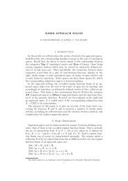
Recently, Siebes and Kersten [16] proposed theGroei algorithm for finding the best k-element Krimpcode table by beam search. By considering a muchlarger search space, they improve over Krimp at expenseof efficiency—for beam-width 1 it coincides withKramp—and hence only small datasets are considered.Although beyond the scope of this paper, theSlim search strategy and estimation heuristics can likelyspeed up Groei significantly.The Pack algorithm [19] makes a connection betweendecision trees and itemsets, mines good decisiontrees, and returns the itemsets that follow from these.It can mine its trees either from a candidate itemsetcollection, or directly from the data. Unlike here, Packconsiders the data 0/1 symmetrically. As a result, itrequires fewer bits, but returns many more itemsets.Wang and Partharsarthy [24] incrementally buildprobabilistic models for predicting itemset frequencies.Iteratively they update the model by those itemsetsfor which the estimate deviated more than the threshold.For efficiency, itemsets are considered in level-wisebatches. Mampaey et al. [11] propose a convex heuristicto efficiently iteratively find the least-well predicteditemset overall, using bic to control complexity. Asconstructing and querying maximum entropy modelsis computationally very expensive, only high-level summariescan be mined. Furthermore, by only consideringfrequency, co-occuring patterns cannot be detected [8].6 ExperimentsHere we experimentally evaluate Slim, its heuristics,and the quality of the discovered code tables.6.1 Setup We implemented a prototype in C++, andprovide the source code for research purposes 2 .We use the shorthand notation L% to denote therelative compressed size of D,L(D, CT )L(D, ST ) %,wherever D is clear from context.As candidates F for Krimp, we use all frequentitemsets mined at the minsup thresholds depicted inTable 1. These thresholds were chosen as low as feasible,while making the processing finish within 24 hours.Krimp includes one of the fastest miners from the FIMIrepository [22]. Timings reported for Krimp includemining and sorting of the candidate collections.All experiments were conducted as single-threadedruns on Linux machines with Intel Xeon X5650 processors(2.66GHz) and 12 GB of memory.2 http://adrem.ua.ac.be/implementations/6.2 Datasets We consider a wide range of benchmarkand real datasets. The base statistics for eachare depicted in Table 1. We show for each database thenumber of attributes, number of transactions, the density(relative number of 1s), and the number of classes.From the LUCS/KDD dataset repository we takesome of the largest and most dense databases. Fromthe FIMI repository we use the Accidents, BMS andPumsb datasets. The Chess (kr–k) and Plants datasetswere obtained from the UCI repository.We use the real Mammals presence and DNA Amplificationdatabases. The former consists of presencerecords of European mammals 3 within geographical areasof 50 × 50 kilometers [13]. The latter contains DNAcopy number amplifications. Such copies activate oncogenesand are hallmarks of advanced tumours [14].From the Antwerp University Hospital we obtainedMCADD data [18]. Medium-Chain Acyl-coenzyme ADehydrogenase Deficiency (MCADD) is a deficiency allnewborns are screened for [20].The Abstracts dataset contains the abstracts of allaccepted papers at the ICDM conference up to 2007,where words are stemmed and stop words removed [8].6.3 Compression First we investigate how wellSlim describes data. In Table 1 we give the relativecompression rates (L%) for both Slim and Krimp. Toease interpretation we also plot these in Figure 1. Theshorter the bars in the plot, the shorter the discovereddescriptions of the data.Overall, we see Slim outperforms Krimp with anaverage gain in compression ratio of 11%, up to over50% for Pumsb. The only exception is BMS-pos, forwhich both methods fail to find succinct descriptions.Analysing these results in more detail, we see that,unsurprisingly, the largest improvements are made onthe large and/or dense datasets, such as Accidents,Connect-4, and Ionosphere. By their characteristics,these datasets give rise to very large numbers of patterns,and hence can only be considered by Krimp ifwe set minsup relatively high—implicitly limiting thedetail at which Krimp can describe the data.The ability to compress a dataset depends on theamount of recognisable structure. For sparse datasets,like Abstracts, and the two BMS datasets, neitherSlim nor Krimp can identify much structure, whereasSlim can describe Pumsb(star) quite succinctly byconsidering lower-frequency itemsets. For dense data,such as Chess (k-k), Connect-4, and Mushroom, bothalgorithms ably find structure.3 The full version of the mammal dataset is available forresearch purposes upon request from the Societas EuropaeaMammalogica. http://www.european-mammals.org

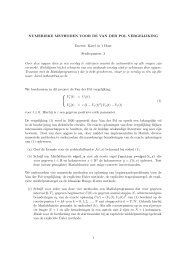
Table 1: Overview statistics.General statistics Krimp SlimDataset |D| |I| %1s |cl| minsup L% |CT | |F| L% |CT | |F|Abstracts 859 3933 1.2 - 3 91.9 1102 6 M 84.3 1815 13 MAccidents 340183 468 7.2 - 50000 55.1 1583 3 M 31.1 2018 21 kAdult 48842 97 15.3 2 1 24.4 1303 58 M 22.8 1201 199 kBMS-pos 515597 1657 0.4 - 100 81.7 9478 6 M 83.1 1964 15 kBMS-webview 1 59602 497 0.5 - 35 85.9 718 1 M 84.0 965 2 MChess (k-k) 3196 75 49.3 2 500 30.0 275 846 M 14.7 292 20 kChess (kr-k) 28056 58 12.1 18 1 61.6 1684 373 k 57.5 1060 28 kConnect-4 67557 129 33.3 3 40000 42.9 56 24 M 12.3 1670 297 kDNA amplification 4590 391 1.5 - 9 36.7 326 312 M 35.7 359 67 kIonosphere 351 157 22.3 2 35 59.8 170 226 M 49.7 240 294 kLetter recognition 20000 102 16.7 26 1 35.7 1780 581 M 33.4 1599 521 kMammals 2183 121 20.5 - 200 48.1 316 94 M 39.9 434 235 kMCADD 31924 198 11.1 2 35 55.4 2280 2 M 51.0 4067 924 kMushroom 8124 119 19.3 2 1 20.5 442 6 G 18.5 340 16 kPen digits 10992 86 19.8 10 1 42.2 1247 459 M 39.4 1347 394 kPlants 34781 70 12.4 - 2000 46.4 511 913 k 36.1 840 179 kPumsb 49046 2113 3.5 - 35000 70.0 175 2 M 19.1 3299 151 kPumsbstar 49046 2088 2.4 - 12500 56.0 331 2 M 25.1 4274 383 kWaveform 5000 101 21.8 3 5 44.5 921 466 M 39.0 734 134 kThe first four columns provide general statistics per dataset; number of transactions, attributes, density (inpercentage of 1s) and number of classes (if any). For Krimp we give relative compression (L%), number ofnon-singleton code table elements, and number of candidates for the given minsup threshold. For Slim we giverelative compression (L%), number of non-singleton code table elements, and number of evaluated candidates.When we look at the number of (non-singleton)itemsets in CT , we see very similar results. In general,for both Slim and Krimp, depending on the data,the code tables contain between a hundred up to afew thousand itemsets. Three datasets, Connect-4 andPumsb-(star), stand-out, with Slim returning 10 timesmore patterns. However, for these Krimp can only runwith very high minsup—whereas Slim does not havethis restriction, and can better capture the structure byusing more fine-grained patterns.6.4 Greedy vs. Greedy Next, we compare Slim totwo variants of the powerful standard greedy optimisationalgorithm for complex combinatorial problems.Kramp is a variant of Krimp that in each iterationchooses that F out of all F that locally maximises compression.Analogously, Slam is a variant of Slim calculatingexact compression gain to order the candidates atevery iteration—instead of estimating it heuristically.Clearly, Slam and Kramp are computationallyexpensive. Hence, we first compare on some small, wellknownUCI benchmark datasets: Anneal, Breast, Heart,Iris, Led7, Nursery, Page blocks, Pima, Tic-tac-toe andWine.All these datasets are easily mined and processedusing a minsup threshold of 1. Comparing the totalcompressed sizes, we observe that Slam is alwaysranked best, Slim second, Kramp third and Krimplast, with an average relative compression (L%) ofrespectively 36.5, 36.8, 37.8 and 40.1. Note thatalthough Kramp considers the largest search-space,it does not always obtain the best result. In theremainder, we do not consider these datasets further.When we consider some larger databases, i.e. Adult,Chess (k-k), DNA, and Letter recog., we see the samepattern: Slam obtains the best average L% of 26.5,Slim a close second at 26.7, and Krimp is behind with31.7—Kramp does not finish within reasonable time.Last, using Adult as a typical example, we plot thedevelopment of L% per itemset accepted into CT asFigure 2. As the plot shows, Slim closely follows Slamand Kramp, quickly converging to good compression—much more directly than Krimp. Note that as itemsetscan be pruned from CT , the final x-coordinate does notnecessarily match |CT | in Table 1. Further, we note thatwhile Slim only needs 35 minutes to converge, Slamrequires one week, and Kramp two months. We willdiscuss convergence and runtime in more detail below.

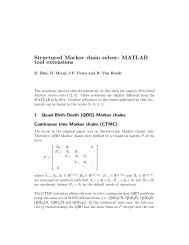
Relative compression (L%)100806040200SlimAbstractsMammalsLetter recog.IonosphereMCADDMushroomPen digitsPlantsPumsbPumsbstarKrimpAccidentsAdultBMS-posBMS-wv1Connect-4Chess (kr-k)(k-k) ChessDNA amp.WaveformTime in seconds10 010 110 210 310 410 5Slim at L% of KrimpFigure 1: Comparing Slim and Krimp: relative compression (L%) (top), overall running time in seconds (bottom),and time needed by Slim to reach the compression attained by Krimp (mid-grey). Note that besides obtainingbetter compression, the Slim prototype is nearly always faster than the optimised Krimp implementation.Relative compression (L%)100908070605040AdultSlimSlamKrimpKrampEstimated ∆L (in bits)3500300025002000150010005000DNA amplificationrejected candidateaccepted candidate100030200 500 1000 1500 2000 2500 3000Number of accepted itemsetsFigure 2: Convergence plot for Adult. The lines in lowerleft corner show the final attained relative compression.−500−100−100 0 100−1000−1000 −500 0 500 1000 1500 2000 2500 3000 3500Exact ∆L (in bits)Figure 3: Correlation plot of the estimated versus exact∆L (in bits) on the DNA amplification dataset.6.5 Number of Candidates Next, we compare thenumber of instantiated candidates |F|, shown in Table1. This is the number of itemsets for which we calculatethe total compressed size by covering the data. ForKrimp this equals the number of frequent itemsets atthe listed minsup threshold. For Slim this reflects thenumber of materialised unions of code table elements.As Table 1 shows, Slim evaluates 2 orders-of-magnitudefewer candidates. In general, Slim considers between 10thousand and 10 million itemsets, whereas Krimp processesmillions to billions of itemsets.Only for Abstracts and BMS-webview 1 Slim evaluatesmore candidates than Krimp—datasets for whicha minute decrease in minsup leads to an explosion ofcandidates. As such, also for this sparse data Slim canconsider candidates at lower support than Krimp canhandle, while for the other datasets Slim only requiresa fraction to reach better compression.

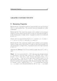
6.6 Timings and convergence We now inspectrun-times and convergence. We plot the total wallclockrunning time for Slim and Krimp as the bottombar plot of Figure 1. For Krimp (darkest bars), thisincludes mining frequent itemsets, sorting, and selectingfrom them. For Slim we mark two timestamps: in midgreywe show the time it takes Slim to overtake Krimp;the light bars display the time to convergence, with amaximum run-time of 24 hours.First we inspect how long Slim requires to matchthe compression of Krimp. We see that for 16 datasetsSlim reaches this point faster than Krimp—in fact,several orders-of-magnitude faster for many of these,particularly for dense datasets. For BMS-pos, thebar is not shown, as Slim does not reach the samecompression. For Ionosphere the bar is simply notvisible, as Slim overtakes Krimp in less than onesecond. As such, Slim is generally much faster thanKrimp in obtaining Krimp-level descriptions.Second, we compare overall runtime. We see Slimis still faster than Krimp for 9 datasets, includinghuge improvements for Chess (k-k), DNA amplification,Ionosphere and Mushroom. For the other datasets,the current implementation requires more time, yet itacquires much more succinct descriptions.To inspect these cases, we again consider Figure 2.By optimising (estimated) gain the compressed sizeconverges much faster for Slim than for Krimp. Afterthe early large gain, the line quickly levels. Althoughnot converged, now only very few bits are gained percandidate. This goes general, where for Pumbsb(star)runtime is further increased by the relatively large codetable. As Slim is worst-case quadratic in |CT |, thetail of convergence is where most time is invested: CTgrows, while few candidates can be pruned. Cachingevaluations between iterations will likely speed up theimplementation. A more efficient encoding would makeselection more strict, providing better descriptions anddo away with the small-gain candidates.In Figure 3 we plot the correlation between ourestimate of ∆L to the actual gain in total compressedsize. We see the two show strong correlation, as mostof the measurements lie on the diagonal, especiallyfor gain (upper right quadrant). Moreover, we seealmost no false positives (upper left quadrant), andonly few examples where few bits are gained while weestimated small loss (lower right quadrant). This strongcorrelation explains why the convergence of Slim andSlam are similar in Figure 2.6.7 Classification Above, we saw Slim describesdata more succinct than Krimp. We here independentlyvalidate how well it captures data distributions byAccuracy (%)1009080706050AdultChess (k-k)Chess (kr-k)Connect-4IonosphereLetter recog.MushroomPen digitsSlimKrimpWaveformFigure 4: Comparing accuracy on classification tasks.classification: Krimp showed performance on par with6 state-of-the-art classifiers on a wide range of datasets[22]. If Slim performs at least as well, we can say itmines code tables at least as characteristic for the data.For this, we reuse the simple classification schemebased on code tables [22]. To use it, we need a code tableper class. To build those we split the database accordingto class, after which the class labels are removed fromall transactions. We then apply Slim and Krimp toeach of these class-databases, resulting in a code tableper class. When the compressors have been constructed,classifying a transaction t is trivial: simply assign theclass label belonging to the code table providing theminimal encoded length for t.We measure performance by accuracy, the percentageof true positives on the test data. All reported resultshave been obtained using 10-fold cross-validation.Note that we do not maximise accuracy by choosinggood pairings between intermediately reported code tables[22], but simply use the final code tables.We give the accuracy scores as Figure 4. Weobserve high similarity between Slim and Krimp, andthat on average Slim performs slightly better. Apair-wise Student t-test reveals that only the resultson the Connect-4 and Chess (kr-k) differ significantly,at significance levels lower than 0.1%, respectively infavour of Slim and Krimp. The performance for Chess(kr-k) is due to Slim much better describing the largeclasses, whereas the more general Krimp code tablesbalance better against those for the small classes.6.8 Outlier Detection To see whether Slim is asuseful as Krimp, we consider a case study on detectingcarriers of MCADD, a rare metabolic disease [18].

Previous work [18] discusses how compression canbe used to identify cases that differ from the norm.Informally said, by building a compressor on a database,we can decide whether a sample is an outlier by itsencoded length: if more bits are required than expected,the sample is likely an outlier. Experiments showKrimp performs on par with the best outlier detectionmethods for binary and categorical data [18].Experiments show Slim provides similar performanceto Krimp: all 8 positive cases are ranked amongthe top-15 using the Slim code tables, and the obtainedperformance indicators (100% sensitivity, 99.9% specificityand a positive predictive value of 53.3%) correspondwith the state-of-the-art results [20].The highly-ranked non-MCADD cases show combinationsof attribute-values very different from the generalpopulation, and are therefore outliers by definition.Analysing the encoding of normal cases reveals thatSlim code tables correctly identify attribute-value combinationscommonly used in diagnostics by experts [20].6.9 Manual Inspection Finally, we subjectivelyevaluate the selected itemsets. To this end, we takeICDM Abstracts dataset. Considering the top-k itemsetswith highest usage we see Slim and Krimp providehighly similar results: both provide patterns relatedto topics in data mining—e.g. ‘mine associationrules [in] databases’, ‘support vector machines (SVM)’,‘algorithm [to] mine frequent patterns’.One can argue, however, that experts should notonly look at the top-ranked itemsets, as the patterns areselected together to describe the data. When we browsethe code tables a whole, we see Slim and Krimp selectroughly the same patterns of 2 to 5 items. As Krimponly considers patterns of at least minsup occurrences,in this data it does not consider more specific itemsets,whereas Slim may consider any itemset in the data.For this dataset, Slim selects a few highly specificpatterns, such as ‘femal, ecologist, jane, goodal,chimpanze, pan, troglodyt, gomb, park, tanzania, riplei,stuctur’. Inspection shows these itemsets all representsmall groups of papers sharing (domain) specificterminology—an application paper in this case—that isnot used in any of the other abstracts. As such, theseitemsets make sense from both interpretation, and MDLperspective; since the likelihood of these words is verylow, yet they strongly interact, and hence can best bedescribed using a single (rare) pattern, saving bits bynot requiring codes for the individual rare words.Note however, that if such level of detail is notdesired, a domain expert can prune the search spaceby specifying additional constraints, e.g. by specifyingminsup, on the candidates Slim may consider.7 DiscussionThe experiments show Slim finds sets of itemsets thatdescribe the data well, characterising it in detail. Inparticular on large and dense datasets, Slim codetables obtain tens of percents better compression ratiothan Krimp. Classification results show high accuracy,verifying that high-quality pattern sets are discovered.Dynamically reconsidering the set of candidateswhile traversing the space leads to better compression.In particular, Slim closely approximates the expensivegreedy algorithms Kramp and Slam, that select thebest candidate of all current candidates. By employinga branch-and-bound strategy using an efficient andtight heuristic, Slim is much more efficient. The goodconvergence adds to its any-time property, providingusers good results within a time-budget, while allowingfurther refinements given more time.Slim generally evaluates two orders-of-magnitudefewer candidates than Krimp, while obtaining moresuccinct descriptions. Moreover, although the Krimpimplementation is optimised, the prototype implementationof Slim is often quicker too. Slim can be optimisedin many ways. For example, we currently donot re-use information from previous iterations; nor dowe cache whether items co-occur at all. Furthermore,Slim is trivial to parallelise, including parallel branchand-boundsearch, evaluation of top-ranked candidates,and covering the data.Although the exact effects on usage of a changein CT can only be calculated by covering the data,better estimates of ∆L may lead to a further decreasein the number of evaluated candidates. Moreover, if theestimate would be sub modular, efficient optimisationstrategies with provable bounds could be employed [15].Our main goal is to provide a faster alternative toKrimp that can operate on large and dense data, whilefinding even better sets of patterns. Both for describingsuccinctly, and classification we have seen Slim is indeedat least as good as Krimp. Further research needs toverify whether Slim can also match or surpass Krimpon other data mining tasks [21, 9, 18].Slim, Slam and Kramp all spend much of theirtime searching for candidates that only lead to minuteimprovements in compression. A natural heuristic tostop search early, without much expected loss of quality,would be to stop as soon as the gain estimate becomesnegative or when a finite difference approximation of thederivative of L% indicates we reach a plateau. Anotheroption is to make selection more strict by refining theencoding model.Although beyond the scope of this paper, the encodingmodel can be improved in several ways. First,by allowing overlap during covering we can likely gain

compression, although covering becomes more complex.Also, dynamic codes could be used; taking into accountwhat itemsets can or cannot be used to encode the remainderof t. These changes will make selection morestrict, increasing convergence, possibly avoiding smallgaincandidates, yet will make encoding more complex.Future work includes investigating whether this indeedleads to better, i.e. more useful, code tables.8 ConclusionIn this paper, we introduced Slim, an any-time algorithmfor mining small, useful, high-quality sets of patternsdirectly from data. We use MDL to identify thebest set of itemsets as that set that describes the databest. To approximate this optimum, we iteratively considerwhat refinement provides most gain—estimatingquality using a light-weight and accurate heuristic. Importantly,Slim is completely parameter-free.Experiments show Slim discovers high-quality patternsets, resulting in high compression rates and highaccuracy scores. Furthermore, Slim closely approximatesthe common greedy approach of selecting the bestcandidate overall, while being several orders faster.There are at least two directions we will explorein future work. Firstly, extending the compressionmodel to allow overlap and use smarter codes. Secondly,optimising our code to analyse even larger data.AcknowledgementsThe authors thank i-ICT of Antwerp University Hospital(uza) for providing data and expertise on MCADD.Koen Smets and Jilles Vreeken are respectively supportedby a Ph.D. and Postdoctoral Fellowship of theResearch Foundation – Flanders (fwo).References[1] R. Agrawal, H. Mannila, R. Srikant, H. Toivonen, andA. I. Verkamo. Fast discovery of association rules. InAdvances in Knowledge Discovery and Data Mining,pp. 307–328. AAAI/MIT Press, 1996.[2] B. Bringmann and A. Zimmermann. The chosen few:On identifying valuable patterns. In Proc. ICDM,pp. 63–72, 2007.[3] T. Calders and B. Goethals. Non-derivable itemsetmining. Data Min. Knowl. Disc., 14(1):171–206, 2007.[4] T. Cover and J. Thomas. Elements of InformationTheory. Wiley-Interscience New York, 2006.[5] F. Geerts, B. Goethals, and T. Mielikäinen. Tilingdatabases. In Proc. DS, pp. 278–289, 2004.[6] P. D. Grünwald. The Minimum Description LengthPrinciple. MIT Press, 2007.[7] A. Knobbe and E. Ho. Pattern teams. In Proc. PKDD,pp. 577–584, 2006.[8] K.-N. Kontonasios and T. De Bie. An informationtheoreticapproach to finding noisy tiles in binarydatabases. In Proc. SDM, pp. 153–164, 2010.[9] M. van Leeuwen, J. Vreeken, and A. Siebes. Identifyingthe components. Data Min. Knowl. Disc., 19(2):173–292, 2009.[10] M. Li and P. Vitányi. An Introduction to KolmogorovComplexity and its Applications. Springer, 1993.[11] M. Mampaey, N. Tatti, and J. Vreeken. Tell me whatI need to know: Succinctly summarizing data withitemsets. In Proc. KDD, pp. 573–581, 2011.[12] T. Mielikäinen and H. Mannila. The pattern orderingproblem. In Proc. PKDD, pp. 327–338, 2003.[13] A. Mitchell-Jones, G. Amori, W. Bogdanowicz,B. Krystufek, P. H. Reijnders, F. Spitzenberger,M. Stubbe, J. Thissen, V. Vohralik, and J. Zima. TheAtlas of European Mammals. Ac. Press, 1999.[14] S. Myllykangas, J. Himberg, T. Böhling, B. Nagy,J. Hollmén, and S. Knuutila. DNA copy numberamplification profiling of human neoplasms. Oncogene,25(55):7324–7332, 2006.[15] G. L. Nemhauser, L. A. Wolsey, and M. L. Fisher. Ananalysis of approximations for maximizing submodularset functions—I. Math. Program., 14:265–294, 1978.[16] A. Siebes and R. Kersten. A structure function fortransaction data. In Proc. SDM, pp. 558–569, 2011.[17] A. Siebes, J. Vreeken, and M. van Leeuwen. Item setsthat compress. In Proc. SDM, pp. 393–404, 2006.[18] K. Smets and J. Vreeken. The Odd One Out: Identifyingand characterising anomalies. In Proc. SDM,pp. 804–815, 2011.[19] N. Tatti and J. Vreeken. Finding good itemsets bypacking data. In Proc. ICDM, pp. 588–597, 2008.[20] T. Van den Bulcke, P. Broucke, V. Hoof, K. Wouters,S. Broucke, G. Smits, E. Smits, S. Proesmans,T. Genechten, and F. Eyskens. Data mining methodsfor classification of Medium-Chain Acyl-CoA dehydrogenasedeficiency (MCADD) using non-derivatized tandemms neonatal screening data. J Biomed Inf, 44:319–325, 2011.[21] J. Vreeken, M. van Leeuwen, and A. Siebes. Characterisingthe difference. In Proc. KDD, pp. 765–774, 2007.[22] J. Vreeken, M. van Leeuwen, and A. Siebes. Krimp:mining itemsets that compress. Data Min. Knowl.Disc., 23(1):169–214, 2011.[23] C. S. Wallace. Statistical and Inductive Inference byMinimum Message Length. Springer, 2005.[24] C. Wang and S. Parthasarathy. Summarizing itemsetpatterns using probabilistic models. In Proc. KDD,pp. 730–735, 2006.[25] G. I. Webb. Discovering significant patterns. Mach.Learn., 68(1):1–33, 2007.[26] G. I. Webb. Self-sufficient itemsets: An approach toscreening potentially interesting associations betweenitems. ACM TKDD, 4(1):1–20, 2010.[27] X. Yan, H. Cheng, J. Han, and D. Xin. Summarizingitemset patterns: a profile-based approach.KDD, pp. 314–323, 2005.In Proc.