Spatial distribution of phytoplankton in the eastern part of the North ...
Spatial distribution of phytoplankton in the eastern part of the North ...
Spatial distribution of phytoplankton in the eastern part of the North ...
- No tags were found...

Create successful ePaper yourself
Turn your PDF publications into a flip-book with our unique Google optimized e-Paper software.
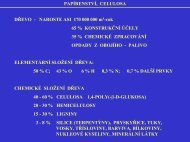
gett<strong>in</strong>g deeper towards <strong>the</strong> north. It <strong>in</strong>cludes <strong>the</strong> Skagerrak with depths up to 725 metres. Surfacewater temperature varies between 0 and 20 °C, depend<strong>in</strong>g on <strong>the</strong> season and <strong>the</strong> <strong>part</strong> <strong>of</strong> <strong>the</strong> sea, withless variation <strong>in</strong> <strong>the</strong> north. Sal<strong>in</strong>ity displays few variations <strong>in</strong> <strong>the</strong> open <strong>North</strong> Sea (32-34.5 ‰). In<strong>the</strong> coastal areas <strong>of</strong> Skagerrak sal<strong>in</strong>ity ranges between 25 and 34 and <strong>in</strong> <strong>the</strong> Wadden Sea it is usuallyless than 30. Temperature and sal<strong>in</strong>ity show variability at annual, seasonal and decadal scales. Thecoastl<strong>in</strong>es display a large variety <strong>of</strong> habitats. In Scotland and Norway <strong>the</strong> coastl<strong>in</strong>es aremounta<strong>in</strong>ous and rocky, <strong>of</strong>ten dissected by deep fjords. The coasts <strong>of</strong> nor<strong>the</strong>rn England andScotland have a variety <strong>of</strong> cliffs, pebble beaches and mud flats. The background <strong>in</strong>formation wastaken from ÆRTEBJERG et al. (2001).2.2. Sampl<strong>in</strong>gSampl<strong>in</strong>g was carried out between 2 nd and 4 th <strong>of</strong> March 2004, with a total <strong>of</strong> n<strong>in</strong>e sampl<strong>in</strong>gstations along a transect, located <strong>in</strong> <strong>the</strong> western, shallow <strong>part</strong> <strong>of</strong> <strong>the</strong> sea (Fig. 1). The stations wereregularly spaced along 55°30´N, between 3°40´E and 7°40´E. The distances between <strong>the</strong> stationswere 30´ (circa 32 km).Figure 1. Location <strong>of</strong> <strong>the</strong> sampl<strong>in</strong>g stations <strong>in</strong> <strong>the</strong> <strong>North</strong> Sea.4
and fixed net samples. For <strong>the</strong> <strong>in</strong>vestigation <strong>of</strong> differences between <strong>the</strong> algal composition <strong>of</strong> bottomand surface water levels, only <strong>the</strong> fixed bottle samples were used.The diatom frustules were cleaned us<strong>in</strong>g <strong>the</strong> follow<strong>in</strong>g procedure: 10 ml <strong>of</strong> <strong>the</strong> sample wasmixed with 2 ml <strong>of</strong> 30% sulphuric acid (H 2 SO 4 ) and 10 ml <strong>of</strong> saturated potassium permanganate(KMnO 4 ). After 24 hours, <strong>the</strong> oxidation was <strong>in</strong>duced by addition <strong>of</strong> 10 ml saturated oxalic acid(H 2 C 2 O 4·2H 2 O). The solution was r<strong>in</strong>sed 3 times with distilled water and a drop was placed onto acoverslip and dried. Afterwards, <strong>the</strong> coverslip was placed onto a slide with a drop <strong>of</strong> Naphraxmount<strong>in</strong>g medium. F<strong>in</strong>ally, <strong>the</strong> slide was carefully heated to remove <strong>the</strong> toluene from <strong>the</strong> medium.Epifluorescence microscopy – For observation <strong>of</strong> <strong>the</strong>cal morphology and plate tabulation <strong>of</strong>d<strong>in</strong>ophyte species, several samples were sta<strong>in</strong>ed with calc<strong>of</strong>luor white solution (FRITZ & TRIEMER1985) and exam<strong>in</strong>ed under <strong>the</strong> Olympus BX-60 microscope equipped with epifluorescenceillum<strong>in</strong>ation lamp Olympus U-RFL-T-200. The UV filter arrangement was for 330-380 nmexcitation and 420 nm emission wavelength (Calc<strong>of</strong>luor absorbs UV radiation <strong>in</strong> <strong>the</strong> 340-400 nmrange and re-emits visible blue light.).Transmission electron microscopy (TEM) – Species <strong>of</strong> choan<strong>of</strong>lagellates and diatoms weredeterm<strong>in</strong>ed us<strong>in</strong>g JEOL 1010 transmission electron microscope. 2 sets <strong>of</strong> grids were used: The gridsmade on board from <strong>the</strong> 10 µm sample and grids from acid-cleaned material. The later was used toexam<strong>in</strong>e frustules <strong>of</strong> small diatoms, which were observed without shadowcast<strong>in</strong>g.Scann<strong>in</strong>g electron microscopy (SEM) – The two samples with <strong>the</strong> highest richness <strong>of</strong> d<strong>in</strong>ophytespecies were exam<strong>in</strong>ed by JEOL JSM-6400 scann<strong>in</strong>g electron microscope. 1 ml <strong>of</strong> <strong>the</strong> Lugol-fixedsample was washed <strong>in</strong> distilled water and mounted on 8 µm Millipore filters. Dehydration throughan ethanol series (15 m<strong>in</strong>utes <strong>in</strong> 30%, 50% and 70% ethanol, 20 m<strong>in</strong>utes <strong>in</strong> 96% ethanol and 30m<strong>in</strong>utes <strong>in</strong> 99% ethanol and 99% ethanol with molecular sieves) was followed by critical-po<strong>in</strong>tdry<strong>in</strong>g with carbon dioxide (BAL-TEC CPD 030). Filters were mounted on 0.5´´ alum<strong>in</strong>iumspecimen stubs (Agar scientific) and sputter-coated with plat<strong>in</strong>um-palladium for 30 seconds us<strong>in</strong>g aJEOL JFC 2300 HR.2.5. Data analysisThe data for species abundance and <strong>the</strong> environmental characteristics were statistically analysedus<strong>in</strong>g a multivariate analysis <strong>in</strong> <strong>the</strong> program Canoco for W<strong>in</strong>dows 4.5 (TER BRAAK & ŠMILAUER1998). The program CanoDraw for W<strong>in</strong>dows 4.0 (TER BRAAK & ŠMILAUER 2002) was used for7
The values varied between 32.7 and 35.0 PSU 1(approximately corresponds to ‰). Higher valueswere observed at <strong>the</strong> stations <strong>in</strong> <strong>the</strong> central <strong>part</strong> <strong>of</strong> <strong>the</strong>sea whereas low sal<strong>in</strong>ity was noted <strong>in</strong> <strong>the</strong> stationsnear <strong>the</strong> coast. This decrease is probably caused by<strong>in</strong>fluence <strong>of</strong> <strong>the</strong> estuaries on <strong>the</strong> west coast <strong>of</strong>Denmark.Dist<strong>in</strong>ct fluctuation <strong>of</strong> fluorescence occurredalong <strong>the</strong> whole transect (Fig. 4). Values <strong>of</strong>chlorophyll a ranged from 0.13 to 0.54 mg/m 3 . Thehighest chlorophyll values were measured at stations157 and 147, located near both ends <strong>of</strong> <strong>the</strong> transect. In<strong>the</strong> middle <strong>part</strong> <strong>of</strong> <strong>the</strong> transect, very low chlorophyllconcentrations were found.Figure 4. Vertical pr<strong>of</strong>ile <strong>of</strong> water fluorescence.3.2. Distribution <strong>of</strong> <strong>the</strong> algal abundanceThere was a dist<strong>in</strong>ct gradient <strong>in</strong> <strong>phytoplankton</strong> concentration <strong>of</strong> cells per ml along <strong>the</strong> wholetransect. The counted concentrations <strong>of</strong> cells are given <strong>in</strong> Tab. 2.Number <strong>of</strong> cells per ml143 145 147 149 151 153 155 157 123Bacillariophyceae 39000 14844 5188 1995 4993 4058 87950 388800 83067Dictyochophyceae 4 4 4 4 21 283 250 36 20D<strong>in</strong>ophyceae 684 244 175 119 50 217 200 144 188Pras<strong>in</strong>ophyceae 4 12 13 0 0 41 0 4 0Chlorophyceae 8 6 6 5 0 0 0 0 0Percentual abundance143 145 147 149 151 153 155 157 123Bacillariophyceae 98.2 98.2 96.3 94.0 98.6 88.2 99.5 100.0 99.8Dictyochophyceae 0.0 0.0 0.1 0.2 0.4 6.2 0.3 0.0 0.0D<strong>in</strong>ophyceae 1.7 1.6 3.2 5.6 1.0 4.7 0.2 0.0 0.2Pras<strong>in</strong>ophyceae 0.0 0.1 0.2 0.0 0.0 0.9 0.0 0.0 0.0Chlorophyceae 0.0 0.0 0.1 0.2 0.0 0.0 0.0 0.0 0.0Table 2. The cell concentrations <strong>of</strong> different <strong>phytoplankton</strong> groups, shown as number <strong>of</strong> cells perml and as a relative percentual abundance.1 PSU means practical sal<strong>in</strong>ity unit, after UNESCOs Practical Sal<strong>in</strong>ity Scale 1978 (FOTONOFF & MILLARD JR. 1983).9
3.3. Phytoplankton composition <strong>of</strong> <strong>the</strong> transectA total <strong>of</strong> 144 different specieswere found at all stations along <strong>the</strong>whole transect. The species list withvalues <strong>of</strong> relative abundances at allstations and references to plates are given<strong>in</strong> Tab. 7 at <strong>the</strong> end <strong>of</strong> <strong>the</strong> document.With 85 species, diatoms were <strong>the</strong>richest group. In comparison, only 44<strong>of</strong> <strong>the</strong> species found wered<strong>in</strong><strong>of</strong>lagellates. O<strong>the</strong>r algal groupsFigure 6. Total species numbers <strong>of</strong> different groups <strong>of</strong>were much less abundant (Fig. 6). The mar<strong>in</strong>e <strong>phytoplankton</strong>, found <strong>in</strong> <strong>the</strong> transect.highest number <strong>of</strong> algal species werefound at stations 153 and 151 (79taxa), located <strong>in</strong> <strong>the</strong> middle <strong>part</strong> <strong>of</strong> <strong>the</strong>transect. At both ends <strong>of</strong> <strong>the</strong> transect,where higher fluorescence wasmeasured, a lower number <strong>of</strong> specieswas found (Fig. 7). This differencewas caused ma<strong>in</strong>ly by changes <strong>in</strong> <strong>the</strong>number <strong>of</strong> d<strong>in</strong><strong>of</strong>lagellate species.Whereas <strong>the</strong> number <strong>of</strong> diatom speciesfound was similar at all stations, <strong>the</strong>Figure 7. <strong>Spatial</strong> variation <strong>in</strong> <strong>the</strong> species number <strong>of</strong>numbers <strong>of</strong> d<strong>in</strong><strong>of</strong>lagellate species were diatoms, d<strong>in</strong><strong>of</strong>lagellates and o<strong>the</strong>r algal groups.highest at stations <strong>in</strong> <strong>the</strong> middle <strong>of</strong> <strong>the</strong>transect.‣ Craspedophyceae – Two species <strong>of</strong> colourless flagellates – Calliacantha simplex andParvicorbicula socialis – were found <strong>in</strong> samples from stations 125 and 153. Both taxa bear anextracellular lorica, which structure serves as important taxonomic feature. The species were foundonly <strong>in</strong> TEM grids, prepared dur<strong>in</strong>g <strong>the</strong> sampl<strong>in</strong>g. Due to <strong>the</strong> small size <strong>of</strong> choan<strong>of</strong>lagellate species11
However, no s<strong>in</strong>gle Chaetocerosspecies was found at all stations. Thespecies C. contortus and C. convolutuswere common at <strong>the</strong> western end <strong>of</strong><strong>the</strong> transect, whereas C. danicus andC. diadema appeared <strong>in</strong> <strong>the</strong> <strong>eastern</strong><strong>part</strong> <strong>of</strong> transect, near <strong>the</strong> coast.Chaetoceros subtilis was observed at Figure 8. <strong>Spatial</strong> variation <strong>in</strong> <strong>the</strong> relative abundance <strong>of</strong><strong>the</strong> stations at both ends <strong>of</strong> <strong>the</strong> transect, four most common species <strong>of</strong> Chaetoceros.but not <strong>in</strong> <strong>the</strong> middle <strong>part</strong>. The genus Thalassiosira was represented by 10 species. Contrary toChaetoceros, some species <strong>of</strong> this genus were found at all stations. The two most common species,T. angulata and T. eccentrica, had maximum relative abundance <strong>in</strong> <strong>the</strong> middle <strong>part</strong> <strong>of</strong> <strong>the</strong> transect.However, <strong>the</strong> highest number <strong>of</strong> species (with very abundant T. nordenskioeldii) was found atstation 143, located near <strong>the</strong> coast. Therefore, <strong>the</strong> middle and <strong>eastern</strong> <strong>part</strong> <strong>of</strong> transect were <strong>the</strong> areaswith <strong>the</strong> highest abundance <strong>of</strong> Thalassiosira species (Fig. 9).The number <strong>of</strong> pennate diatomspecies was clearly less than centricones (only 25 % <strong>of</strong> all species),although some species occurred <strong>in</strong>high abundance. Among <strong>the</strong> mostabundant species were Nitzschialongissima and Thalassionemanitzschioides. High levels <strong>of</strong>fluorescence <strong>in</strong> <strong>the</strong> <strong>eastern</strong> <strong>part</strong> <strong>of</strong> <strong>the</strong>transect were probably caused by <strong>the</strong>irFigure 9. <strong>Spatial</strong> variation <strong>in</strong> <strong>the</strong> relative abundanceblooms. O<strong>the</strong>r pennate diatom species, <strong>of</strong> Thalassiosira species.Asterionellopsis glacialis and Pseudonitzschiapungens, were very frequent at stations <strong>in</strong> <strong>the</strong> western <strong>part</strong> <strong>of</strong> <strong>the</strong> transect. Cells <strong>of</strong>Rhaphoneis amphiceros appeared <strong>in</strong> quite high abundance at all stations. They were observed <strong>in</strong>plankton attached to sand gra<strong>in</strong>s or to <strong>the</strong> frustules <strong>of</strong> o<strong>the</strong>r diatoms.A high number <strong>of</strong> species belonged to <strong>the</strong> genera Navicula and Nitzschia. In total, 9 species <strong>of</strong>Navicula were identified. Navicula distans was <strong>the</strong> most common species. The Nitzschia genus13
was represented by 6 species, with <strong>the</strong>most common species, be<strong>in</strong>g Nitzschialongissima and N. constricta. Along<strong>the</strong> transect, dist<strong>in</strong>ct changes <strong>in</strong>Nitzschia abundance was observed.Whereas all species were observed <strong>in</strong><strong>the</strong> western <strong>part</strong>, only N. longissimaoccurred on <strong>the</strong> <strong>eastern</strong> side <strong>of</strong> <strong>the</strong>transect (Fig. 10).Figure 10. <strong>Spatial</strong> variation <strong>in</strong> <strong>the</strong> relative abundance‣ D<strong>in</strong>ophyceae – A total <strong>of</strong> 44 <strong>of</strong> Nitzschia species.different species <strong>of</strong> d<strong>in</strong><strong>of</strong>lagellates were found <strong>in</strong> <strong>the</strong> transect. The most abundant species wereAlexandrium tamarense <strong>in</strong> <strong>the</strong> western <strong>part</strong>, Protoperid<strong>in</strong>ium achromaticum and Diplopelta bomba<strong>in</strong> <strong>the</strong> <strong>eastern</strong> <strong>part</strong>, and Pentapharsod<strong>in</strong>ium dalei at all stations along <strong>the</strong> transect with maximumabundance <strong>in</strong> <strong>the</strong> central area. At all stations, M<strong>in</strong>uscula bipes, Protoperid<strong>in</strong>ium pellucidum andZygabikod<strong>in</strong>ium lenticulatum occurred <strong>in</strong> relatively constant abundance.Most <strong>of</strong> <strong>the</strong> d<strong>in</strong><strong>of</strong>lagellate species found belong to <strong>the</strong> <strong>the</strong>cate genera Ceratium andProtoperid<strong>in</strong>ium (only 5 a<strong>the</strong>cate species were found). In total, 7 species <strong>of</strong> Ceratium occurred <strong>in</strong><strong>the</strong> transect, with a dist<strong>in</strong>ct gradient <strong>of</strong> abundance. All 7 species were found <strong>in</strong> <strong>the</strong> central area,while no species <strong>of</strong> this genus were found at two stations <strong>in</strong> <strong>the</strong> western <strong>part</strong> <strong>of</strong> <strong>the</strong> transect (Fig.11). A similar decrease <strong>in</strong> number <strong>of</strong> species was noted <strong>in</strong> <strong>the</strong> <strong>eastern</strong> end <strong>of</strong> transect, where only 2species occurred.With 17 species found, <strong>the</strong> genusProtoperid<strong>in</strong>ium was <strong>the</strong> richest genus<strong>of</strong> algae, and was found throughout <strong>the</strong>transect. P. achromaticum, <strong>the</strong> mostnumerous species, was very abundantat stations 143 and 145, located near<strong>the</strong> coast. After Thalassionemanitzschioides, P. achromaticum was Figure 11. <strong>Spatial</strong> variation <strong>in</strong> <strong>the</strong> relative abundance<strong>of</strong> Ceratium species.<strong>the</strong> second most dom<strong>in</strong>ant alga <strong>in</strong><strong>the</strong>se samples. However, <strong>the</strong>re were no cells found at <strong>the</strong> western end <strong>of</strong> <strong>the</strong> transect. Interest<strong>in</strong>gly,only P. pellucidum occurred at all stations along <strong>the</strong> transect. All o<strong>the</strong>r species appeared ei<strong>the</strong>r <strong>in</strong>14
<strong>part</strong> <strong>of</strong> <strong>the</strong> transect (e.g. P. pyriformeor P. sub<strong>in</strong>erme) or only at one station(e.g. P. marielebouriae, quite commonat station 145, but not found at nearbystations). Generally, <strong>the</strong> highestoccurrence <strong>of</strong> Protoperid<strong>in</strong>ium specieswas noted at stations 153 and 151, <strong>in</strong><strong>the</strong> central <strong>part</strong> <strong>of</strong> <strong>the</strong> transect.Towards both ends <strong>of</strong> <strong>the</strong> transect,decreas<strong>in</strong>g total relative abundance <strong>of</strong> Figure 12. <strong>Spatial</strong> variation <strong>in</strong> <strong>the</strong> relative abundancespecies was noted. Only at <strong>the</strong> coastal <strong>of</strong> Protoperid<strong>in</strong>ium species.station 145, high abundance <strong>of</strong> P. achromaticum toge<strong>the</strong>r with <strong>the</strong> presence <strong>of</strong> 3 unique speciescaused <strong>the</strong> <strong>in</strong>crease <strong>of</strong> species abundance (Fig. 12).‣ Pras<strong>in</strong>ophyceae – In total, 5 species belong<strong>in</strong>g to this group were found <strong>in</strong> <strong>the</strong> transect.A<strong>part</strong> from Halosphaera viridis, found <strong>in</strong> <strong>the</strong> western <strong>part</strong> <strong>of</strong> <strong>the</strong> transect, all o<strong>the</strong>r species belongedto <strong>the</strong> genus Pterosperma. Species <strong>of</strong>this genus are ma<strong>in</strong>ly dist<strong>in</strong>guished by<strong>the</strong> structure <strong>of</strong> <strong>the</strong> phycoma stage,bear<strong>in</strong>g a dist<strong>in</strong>ct equatorial keel or asystem <strong>of</strong> keels, divid<strong>in</strong>g its surface<strong>in</strong>to polygons. Pterosperma cristatum,appeared <strong>in</strong> <strong>the</strong> western and central<strong>part</strong>s <strong>of</strong> <strong>the</strong> transect, and <strong>the</strong> threeo<strong>the</strong>r species were found only <strong>in</strong> <strong>the</strong>central <strong>part</strong> <strong>of</strong> <strong>the</strong> study area (Fig. 13). Figure 13. <strong>Spatial</strong> variation <strong>in</strong> <strong>the</strong> relative abundance<strong>of</strong> Pterosperma species.This is <strong>in</strong> accordance with cellabundance, which was highest <strong>in</strong> <strong>the</strong> same, central area <strong>of</strong> <strong>the</strong> transect (Fig. 5c).‣ Chlorophyceae – Only three species <strong>of</strong> this group were found – Pediastrum boryanum,Pediastrum cf. kawraiskyi and Scenedesmus sp. Pediastrum boryanum was found at <strong>the</strong> six stations<strong>in</strong> <strong>the</strong> <strong>eastern</strong> <strong>part</strong> <strong>of</strong> <strong>the</strong> transect, while Scenedesmus sp. and Pediastrum cf. kawraiskyi were onlyfound at stations 145 and 143, respectively, nearest <strong>the</strong> coast.15
3.4. Differences <strong>in</strong> algal composition <strong>of</strong> bottom and surface water levelsAt four stations (every second station <strong>in</strong> <strong>the</strong> transect), <strong>the</strong> differences between bottom andsurface species composition were <strong>in</strong>vestigated. In this survey, a total <strong>of</strong> 70 species was foundaltoge<strong>the</strong>r at <strong>the</strong> four stations (46 diatoms, 17 d<strong>in</strong><strong>of</strong>lagellates, 7 species belong<strong>in</strong>g to o<strong>the</strong>r groups <strong>of</strong>algae). Most species exhibited <strong>the</strong> same abundance <strong>in</strong> both bottom and surface water samples,however several species, <strong>in</strong> <strong>the</strong> two largest groups <strong>of</strong> algae, showed a dist<strong>in</strong>ct vertical gradient. Therelative abundances <strong>of</strong> species, occurred <strong>in</strong> <strong>the</strong> bottom and surface water samples, are given <strong>in</strong> Tab. 8.Interest<strong>in</strong>gly, several diatoms were found to be more abundant <strong>in</strong> bottom water samples(Asterionellopsis glacialis, Pleurosigma lanceolatum, Neostrepto<strong>the</strong>ca sub<strong>in</strong>dica and Nitzschialongissima), while only Podosira stelliger was found more <strong>of</strong>ten <strong>in</strong> surface water samples. Theopposite pattern was found <strong>in</strong> two d<strong>in</strong><strong>of</strong>lagellate species (Ceratium l<strong>in</strong>eatum and Protoperid<strong>in</strong>iumachromaticum), which were more abundant <strong>in</strong> surface water samples. No d<strong>in</strong><strong>of</strong>lagellate speciesoccurred with higher abundance <strong>in</strong> bottom water samples.In Fig. 14, show<strong>in</strong>g <strong>the</strong> vertical gradient <strong>of</strong> diatom species abundance, <strong>the</strong> greatest differencebetween bottom and surface water species composition is apparent at station 153. There, <strong>the</strong> totalnumber <strong>of</strong> species occurr<strong>in</strong>g <strong>in</strong> surface or bottom water samples was 24 and 30, respectively. At <strong>the</strong>same station, <strong>the</strong> <strong>in</strong>verse vertical gradient <strong>of</strong> d<strong>in</strong><strong>of</strong>lagellate species was noted (Fig. 15). Due to <strong>the</strong>very small number <strong>of</strong> species found from o<strong>the</strong>r algal classes, vertical gradients were <strong>in</strong>terpretedonly for <strong>the</strong> two previously mentioned algal groups.Figure 14. Horizontal and vertical variation<strong>in</strong> <strong>the</strong> number <strong>of</strong> diatom species found. Redcolour <strong>in</strong>dicates <strong>the</strong> areas with <strong>the</strong> highestspecies richness.Figure 15. Horizontal and vertical variation<strong>in</strong> <strong>the</strong> number <strong>of</strong> d<strong>in</strong><strong>of</strong>lagellate speciesfound. Red colour <strong>in</strong>dicates <strong>the</strong> areas with<strong>the</strong> highest species richness.16
3.5. Results <strong>of</strong> statistical analyses3.5.1. Inner structure <strong>of</strong> dataAn <strong>in</strong>direct gradient analysis PCA was used to detect <strong>the</strong> <strong>in</strong>ner structure <strong>of</strong> <strong>the</strong> data obta<strong>in</strong>ed.The results are given <strong>in</strong> Tab. 3:**** Summary ****Axes 1 2 3 4 Total varianceEigenvalues : 0.386 0.214 0.123 0.096 1.000Cumulative percentage variance <strong>of</strong> species data : 38.6 60.0 72.3 81.8Sum <strong>of</strong> all eigenvalues 1.000Table 3. Part <strong>of</strong> <strong>the</strong> PCA analysis output.The two first ord<strong>in</strong>ation axes toge<strong>the</strong>rexpla<strong>in</strong>ed 60 % <strong>of</strong> <strong>the</strong> total variability.The positions <strong>of</strong> <strong>the</strong> samples <strong>in</strong> <strong>the</strong> space<strong>of</strong> <strong>the</strong>se two axes are illustrated <strong>in</strong> Fig. 16.On <strong>the</strong> ord<strong>in</strong>ation diagram, <strong>the</strong> sampl<strong>in</strong>glocalities are arranged more or less <strong>in</strong>correspondence to <strong>the</strong>ir physical orderalong transect, form<strong>in</strong>g <strong>the</strong> shape <strong>of</strong> anoverturned letter U. The sampl<strong>in</strong>g stationsform three dist<strong>in</strong>ct groups <strong>in</strong> <strong>the</strong> diagram: Figure 16. Positions <strong>of</strong> <strong>the</strong> samples <strong>in</strong> <strong>the</strong> space <strong>of</strong><strong>the</strong> first two ord<strong>in</strong>ation axes. PCA analysis.The group <strong>of</strong> coastal stations 143, 145,147 and 149; <strong>the</strong> group <strong>of</strong> oceanic stations 123, 155 and 157; and <strong>the</strong> group <strong>of</strong> two stations 151 and153, situated <strong>in</strong> <strong>the</strong> middle <strong>part</strong> <strong>of</strong> <strong>the</strong> transect. Dist<strong>in</strong>ct separation <strong>of</strong> <strong>the</strong>se three groups along <strong>the</strong>first ord<strong>in</strong>ation axis reflects to <strong>the</strong> important role <strong>of</strong> <strong>the</strong> distance from <strong>the</strong> coast for <strong>the</strong> speciescomposition at each station. However, <strong>the</strong> uneven arrangement <strong>of</strong> <strong>the</strong> stations along <strong>the</strong> first axis<strong>in</strong>dicates <strong>the</strong> considerable changes <strong>of</strong> <strong>phytoplankton</strong> composition <strong>in</strong> <strong>the</strong> areas between stations 149-151 and 153-155.The ratio <strong>of</strong> species composition <strong>of</strong> <strong>the</strong> samples and <strong>the</strong> orientation <strong>of</strong> environmental variables<strong>in</strong> ord<strong>in</strong>ation space are shown <strong>in</strong> Fig. 17. The association <strong>of</strong> coastal distance with <strong>the</strong> first axis iswell shown. Similarly, <strong>the</strong> second ord<strong>in</strong>ation axis divid<strong>in</strong>g <strong>the</strong> stations 151 and 153 from all o<strong>the</strong>r17
ones is l<strong>in</strong>ked positively with <strong>the</strong> depth <strong>of</strong> seaand negatively with fluorescence. At stations,sited <strong>in</strong> negative <strong>part</strong> <strong>of</strong> second ord<strong>in</strong>ationaxis (stations 123, 157, 143), high values <strong>of</strong>fluorescence were measured. At <strong>the</strong> samestations, <strong>the</strong>re were also higher numbers <strong>of</strong>diatom species.Figure 17. Positions <strong>of</strong> <strong>the</strong> samples and <strong>the</strong>environmental variables <strong>in</strong> <strong>the</strong> space <strong>of</strong> <strong>the</strong>first two ord<strong>in</strong>ation axes. PCA analysis. Theratio <strong>of</strong> <strong>the</strong> species composition <strong>of</strong> allsamples is shown (yellow – diatoms, green –d<strong>in</strong><strong>of</strong>lagellates, grey – o<strong>the</strong>rs).-1.0 1.0coast145149147143151depthfluorescence-1.0 1.0153123temperaturesal<strong>in</strong>ity155abundance1573.5.2. Relationships between <strong>phytoplankton</strong> and environmental characteristicsThe <strong>in</strong>fluence <strong>of</strong> several environmental characteristics on species composition was statisticallytested us<strong>in</strong>g RDA analysis. Separate analyses were made to detect <strong>the</strong> <strong>in</strong>fluence <strong>of</strong> temperature,sal<strong>in</strong>ity, fluorescence, distance from <strong>the</strong> coast, depth and <strong>the</strong> total abundance <strong>of</strong> algae. Interest<strong>in</strong>gly,only <strong>the</strong> <strong>in</strong>fluence <strong>of</strong> distance from coast proved to be significant, with a p-value <strong>of</strong> 0.001. All o<strong>the</strong>rcharacteristics here found not to be statistically significant for <strong>the</strong> transect. The results <strong>of</strong> analysiswith distance from <strong>the</strong> coast as <strong>the</strong> tested environmental variable are given <strong>in</strong> Tab. 4.**** Summary ****Axes 1 2 3 4 Total varianceEigenvalues : 0.343 0.201 0.132 0.090 1.000Species-environment correlations : 0.972 0.000 0.000 0.000Cumulative percentage variance<strong>of</strong> species data : 34.3 54.4 67.6 76.6<strong>of</strong> species-environment relation : 100.0 0.0 0.0 0.0Sum <strong>of</strong> all eigenvalues 1.000Sum <strong>of</strong> all canonical eigenvalues 0.343**** Summary <strong>of</strong> Monte Carlo test ****Test <strong>of</strong> significance <strong>of</strong> all canonical axes: Trace = 0.343F-ratio = 3.658P-value = 0.0010Table 4. Part <strong>of</strong> <strong>the</strong> RDA analysis output.18
The first ord<strong>in</strong>ation axis, characteriz<strong>in</strong>g <strong>the</strong> <strong>in</strong>fluence <strong>of</strong> coast distance, expla<strong>in</strong>ed almost 35 %<strong>of</strong> <strong>the</strong> total variability. In Fig. 18., <strong>the</strong> relation <strong>of</strong> <strong>in</strong>dividual species to <strong>the</strong> coastal or oceanicenvironment is shown. The species names abbreviations, used <strong>in</strong> follow<strong>in</strong>g figure, are given <strong>in</strong> Tab. 5.Figure 18. Positions <strong>of</strong> <strong>the</strong> species and <strong>the</strong>ir relation to <strong>the</strong> coastal or oceanic environment <strong>in</strong> <strong>the</strong> space<strong>of</strong> <strong>the</strong> first two ord<strong>in</strong>ation axes. RDA analysis. The 78 most fitted species are shown <strong>in</strong> <strong>the</strong> diagram.The species with aff<strong>in</strong>ity to coastal environment are situated <strong>in</strong> <strong>the</strong> right <strong>part</strong> <strong>of</strong> <strong>the</strong> diagram.Chaetoceros diadema, Chaetoceros danicus, Emiliania huxleyi, Protoperid<strong>in</strong>ium achromaticum,Act<strong>in</strong>optychus senarius and Pediastrum boryanum belong among <strong>the</strong> typical coastal species.Similarly, 5 <strong>of</strong> 6 species <strong>of</strong> Thalassiosira, shown <strong>in</strong> <strong>the</strong> diagram, are positively correlated withcoastal environment. The species Chaetoceros convolutus, Chaetoceros contortus, Pleurosigmalanceolatum, Gyrosigma fascicola, Skeletonema costatum and o<strong>the</strong>r species <strong>in</strong> <strong>the</strong> left <strong>part</strong> <strong>of</strong>diagram show an aff<strong>in</strong>ity for oceanic environment. Species displayed <strong>in</strong> <strong>the</strong> upper <strong>part</strong> <strong>of</strong> <strong>the</strong>19
4. DiscussionAlong <strong>the</strong> transect, vertical and horizontal gradients <strong>of</strong> algal concentration and species numberwere found. Three groups <strong>of</strong> stations were found based on different <strong>phytoplankton</strong> composition:Most <strong>of</strong> <strong>the</strong> species were most abundant ei<strong>the</strong>r at <strong>the</strong> coastal or at <strong>the</strong> oceanic end <strong>of</strong> <strong>the</strong> transect,while some species occurred ma<strong>in</strong>ly at stations located <strong>in</strong> <strong>the</strong> deeper area <strong>in</strong> <strong>the</strong> middle <strong>of</strong> <strong>the</strong>transect. High concentrations <strong>of</strong> diatom cells per ml were noted at both ends <strong>of</strong> <strong>the</strong> transect.However, <strong>the</strong> algal composition <strong>of</strong> stations situated at <strong>the</strong> <strong>eastern</strong> and <strong>the</strong> western end <strong>of</strong> <strong>the</strong>transect, respectively, were different. Generally, <strong>the</strong> highest species diversity <strong>of</strong> all algae groupswas found at station with <strong>the</strong> lowest number <strong>of</strong> algae per ml. This phenomenon is known not onlyfrom mar<strong>in</strong>e environment but also from all types <strong>of</strong> natural conditions, as has been published e. g.by LEVIN et al. (2001). A vertical gradient <strong>in</strong> species number <strong>of</strong> diatoms and d<strong>in</strong><strong>of</strong>lagellates wasfound <strong>in</strong> <strong>the</strong> middle <strong>part</strong> <strong>of</strong> <strong>the</strong> transect. The gradient was probably caused by slight stratification,appeared as small vertical gradients <strong>of</strong> temperature and sal<strong>in</strong>ity at station 151 (Figs 2., 3.).The level <strong>of</strong> temperature and sal<strong>in</strong>ity was more or less constant along <strong>the</strong> whole transect, a<strong>part</strong>from two stations at <strong>the</strong> west coast <strong>of</strong> Denmark. There <strong>the</strong> water was colder and less sal<strong>in</strong>e probablydue to <strong>the</strong> <strong>in</strong>fluence <strong>of</strong> fresh water from estuaries along <strong>the</strong> coast <strong>of</strong> Denmark. A very differentpattern was found <strong>in</strong> <strong>the</strong> spatial <strong>distribution</strong> <strong>of</strong> fluorescence values. Two dist<strong>in</strong>ct peaks <strong>of</strong>fluorescence occurred at stations 157 and 147, located at <strong>the</strong> opposite ends <strong>of</strong> <strong>the</strong> transect. In <strong>the</strong>middle <strong>part</strong> <strong>of</strong> <strong>the</strong> transect, very low chlorophyll concentrations were found. This <strong>distribution</strong> <strong>of</strong>chlorophyll was obviously associated with <strong>the</strong> water depth. High values <strong>of</strong> chlorophyll weremeasured <strong>in</strong> <strong>the</strong> shallow <strong>part</strong>s <strong>of</strong> <strong>the</strong> transect, while <strong>in</strong> <strong>the</strong> deepest <strong>part</strong> (station 151) <strong>the</strong> lowestconcentration was found. While <strong>the</strong> <strong>eastern</strong> end <strong>of</strong> <strong>the</strong> transect was <strong>in</strong>fluenced by coastal proximity,<strong>the</strong> small depth at <strong>the</strong> western end <strong>of</strong> <strong>the</strong> transect was caused by <strong>the</strong> vic<strong>in</strong>ity <strong>of</strong> <strong>the</strong> shallow areaDogger Bank (JOHNS & REID 2001). These two zones were separated by an area with depths <strong>of</strong> 35 –40 meters. The high algal abundance at both ends <strong>of</strong> <strong>the</strong> transect was probably caused by <strong>the</strong>nutrients richness <strong>in</strong> shallow, mixed <strong>part</strong>s <strong>of</strong> <strong>the</strong> sea, that evoked <strong>the</strong> <strong>phytoplankton</strong> bloom.However, we did not measure any nutrients concentrations to support this hypo<strong>the</strong>sis.At both ends <strong>of</strong> <strong>the</strong> transect, <strong>the</strong> high values <strong>of</strong> fluorescence were probably caused by <strong>the</strong> largenumber <strong>of</strong> diatoms, which are typical organisms <strong>of</strong> spr<strong>in</strong>g blooms <strong>in</strong> mar<strong>in</strong>e environments (JOHNS& REID 2001). However, we could not absolutely rule out that <strong>the</strong>se values were caused by o<strong>the</strong>rorganisms, for example by those, which are nanoplanktonic. They could contribute to <strong>the</strong> measured21
values <strong>of</strong> fluorescence but <strong>the</strong>y were not found. However, diatoms seemed to be really dom<strong>in</strong>antorganisms, because we found <strong>the</strong>m <strong>in</strong> huge numbers, for example circa 400 millions cells per litre<strong>of</strong> sampled water at station 157. Moreover, <strong>the</strong> diatom blooms at <strong>the</strong> different ends <strong>of</strong> <strong>the</strong> transectwere produced by different species. At <strong>the</strong> <strong>eastern</strong> end <strong>of</strong> <strong>the</strong> transect, <strong>the</strong> diatoms Porosiraglacialis, Thalassionema nitzschioides and Thalassiosira nordenskioeldii were dom<strong>in</strong>ant. Incontrast, <strong>the</strong> bloom at <strong>the</strong> western end <strong>of</strong> <strong>the</strong> transect was ma<strong>in</strong>ly caused by Skeletonema costatum,Nitzschia longissima and Porosira glacialis. The spatial <strong>distribution</strong> <strong>of</strong> Porosira glacialis showedan atypical pattern, with high abundances at both ends <strong>of</strong> <strong>the</strong> transect. Such a <strong>distribution</strong> was notfound <strong>in</strong> any o<strong>the</strong>r algal species. Some o<strong>the</strong>r species, e.g. Cosc<strong>in</strong>odiscus asteromphalus andPleurosigma normanii, occurred with almost same abundance at all stations.The bloom <strong>of</strong> Skeletonema costatum <strong>in</strong> <strong>the</strong> sea far from <strong>the</strong> coast is quite surpris<strong>in</strong>g. Occurrence<strong>of</strong> Skeletonema costatum is usually associated with <strong>the</strong> coastal areas; blooms have been reportedvery frequently dur<strong>in</strong>g spr<strong>in</strong>g from <strong>the</strong> coastal areas <strong>in</strong> Norway (BRAARUD et al. 1973; ERGA &HEIMDAL 1984), Canada (CONOVER & MAYZAUD 1984), Alaska (WAITE et al. 1992) and BritishColumbia (HAIGH et al. 1992). Fur<strong>the</strong>rmore, SMAYDA (1957) suggested that Skeletonema costatumgrows best <strong>in</strong> semi-enclosed waters and it is not <strong>of</strong>ten found <strong>in</strong> high concentrations <strong>in</strong> oceanicenvironments. In our study, high abundances were noted at stations near <strong>the</strong> coast. However, <strong>the</strong>highest abundance <strong>of</strong> this species was observed at <strong>the</strong> western end <strong>of</strong> <strong>the</strong> transect, <strong>in</strong> <strong>the</strong> middle <strong>part</strong><strong>of</strong> <strong>the</strong> <strong>North</strong> Sea. Additionally, <strong>the</strong> diatom cell concentration <strong>in</strong> this <strong>part</strong> <strong>of</strong> transect was 10x higherthan <strong>the</strong> bloom near <strong>the</strong> coast. The high production <strong>of</strong> Skeletonema costatum <strong>in</strong> <strong>the</strong> open sea mightbe caused by <strong>the</strong> relatively shallow water <strong>in</strong> this <strong>part</strong> <strong>of</strong> <strong>the</strong> sea, which simulates coastal conditions,and <strong>the</strong> slightly warmer water temperature. The higher oceanic abundance could be also associatedwith eddies reflect<strong>in</strong>g <strong>the</strong> coastal orig<strong>in</strong> <strong>of</strong> <strong>the</strong> water. However, our data did not support <strong>the</strong>hypo<strong>the</strong>sis about ecological preference <strong>of</strong> S. costatum for semi-enclosed, coastal waters, as has beenproposed by SMAYDA (1957).The spatial <strong>distribution</strong> <strong>of</strong> d<strong>in</strong><strong>of</strong>lagellates was similar to that <strong>of</strong> diatoms. However, <strong>the</strong> highestnumber <strong>of</strong> d<strong>in</strong><strong>of</strong>lagellate cells was found at station 143, whereas <strong>the</strong> highest bloom <strong>of</strong> diatoms wasobserved at station 157. The lowest abundance <strong>of</strong> d<strong>in</strong><strong>of</strong>lagellates was found <strong>in</strong> <strong>the</strong> middle <strong>of</strong> <strong>the</strong>transect (station 151). It <strong>in</strong>creased aga<strong>in</strong> toward <strong>the</strong> oceanic end <strong>of</strong> <strong>the</strong> transect. The speciescompositions <strong>of</strong> <strong>the</strong> coastal and oceanic ends <strong>of</strong> transect were also different. Among <strong>the</strong> speciesfound more <strong>in</strong> <strong>the</strong> coastal area were ma<strong>in</strong>ly Protoperid<strong>in</strong>ium achromaticum, Phalacromarotundatum, Prorocentrum micans and most species <strong>of</strong> <strong>the</strong> genus Ceratium. Protoperid<strong>in</strong>ium22
achromaticum has previously been found by e. g. DODGE (1982) from British Isles and byTRIGUEROS et al. (2000) <strong>in</strong> <strong>the</strong> estuary <strong>of</strong> Urdaibai <strong>in</strong> nor<strong>the</strong>rn Spa<strong>in</strong>. It seems that this species isable to tolerate wide range <strong>of</strong> sal<strong>in</strong>ity <strong>in</strong> mar<strong>in</strong>e and brackish waters. The species found ma<strong>in</strong>ly at<strong>the</strong> oceanic end <strong>of</strong> <strong>the</strong> transect were Protoceratium reticulatum, Protoperid<strong>in</strong>ium cerasus andProtoperid<strong>in</strong>ium pyriforme. M<strong>in</strong>uscula bipes, Pentapharsod<strong>in</strong>ium dalei, Protoperid<strong>in</strong>iumpellucidum and Zygabikod<strong>in</strong>ium lenticulatum were found at all stations <strong>of</strong> <strong>the</strong> transect, but <strong>the</strong>ircontribution to <strong>the</strong> total quantity <strong>of</strong> algae was ra<strong>the</strong>r low.The species <strong>of</strong> <strong>the</strong> genus Dictyocha (ma<strong>in</strong>ly <strong>the</strong> species D. speculum) showed a different spatial<strong>distribution</strong> along <strong>the</strong> transect. Contrary to diatoms and d<strong>in</strong><strong>of</strong>lagellates, <strong>the</strong>y were ma<strong>in</strong>ly found <strong>in</strong><strong>the</strong> middle <strong>part</strong> <strong>of</strong> <strong>the</strong> transect. Only <strong>the</strong> skeleton bear<strong>in</strong>g stadium was found <strong>in</strong> all samples,although this genus is able to form o<strong>the</strong>r stages, which don’t require silicate and <strong>the</strong>refore don’tcompete with diatoms for it.Three dist<strong>in</strong>ct groups <strong>of</strong> stations were found based on differences <strong>in</strong> species composition – threestations at each end <strong>of</strong> <strong>the</strong> transect, and two stations <strong>in</strong> <strong>the</strong> middle. Different algal speciesdom<strong>in</strong>ated <strong>in</strong> each group. <strong>Spatial</strong> differences <strong>of</strong> <strong>phytoplankton</strong> composition along <strong>the</strong> transect wassignificant <strong>in</strong> RDA analysis, show<strong>in</strong>g differences between coastal and oceanic species. REID et al.(1978), who <strong>in</strong>vestigated <strong>the</strong> spatial <strong>distribution</strong> <strong>of</strong> <strong>phytoplankton</strong> <strong>of</strong>California, published similar results. They found that <strong>the</strong> planktoncomposition at stations 100 km a<strong>part</strong> <strong>in</strong> <strong>the</strong> along shore direction wasmore similar that at stations hundreds <strong>of</strong> meters a<strong>part</strong> <strong>in</strong> <strong>the</strong> <strong>of</strong>fshoredirection.The dependence <strong>of</strong> depth, sal<strong>in</strong>ity, temperature and fluorescenceon <strong>the</strong> species composition was not proved. For illustration, <strong>the</strong> p-values from <strong>the</strong> results <strong>of</strong> RDA analyses are given <strong>in</strong> Tab. 6.environmentalvariablesp-valuescoast 0.001depth 0.18temperature 0.29sal<strong>in</strong>ity 0.41fluorescence 0.69Table 6. The results <strong>of</strong>Monte-Carlo permutationtests <strong>of</strong> all environmentalvariables.The <strong>in</strong>dividual species showed four types <strong>of</strong> <strong>distribution</strong> along <strong>the</strong> transect, as shown <strong>in</strong> Fig. 18(coastal, oceanic, with a maximum <strong>of</strong> abundance <strong>in</strong> <strong>the</strong> middle <strong>part</strong> <strong>of</strong> <strong>the</strong> transect, or moreabundant at both ends <strong>of</strong> <strong>the</strong> transect.). Most <strong>of</strong> <strong>the</strong> species occurred <strong>in</strong> ei<strong>the</strong>r <strong>the</strong> <strong>eastern</strong> or <strong>the</strong>western <strong>part</strong> <strong>of</strong> <strong>the</strong> transect, <strong>in</strong> coastal or open oceanic environment, respectively. With <strong>the</strong>exception <strong>of</strong> Skeletonema costatum, <strong>the</strong> ecological preferences <strong>of</strong> most o<strong>the</strong>r species correspondwith published data. A preference for coastal environment has previously been published for e. g.Cosc<strong>in</strong>odiscus wailesii (EDWARDS & JOHNS 2002), Emiliania huxleyi (YANG et al. 2001), andThalassiosira angulata and T. nordenskioeldii (REIGSTAD et al. 2000). The genus Chaetoceros is,23
5. ConclusionsThe data for this survey were obta<strong>in</strong>ed dur<strong>in</strong>g <strong>the</strong> cruise <strong>of</strong> <strong>the</strong> vessel Dana through <strong>the</strong> <strong>North</strong>Sea <strong>in</strong> March 2004. Samples were collected at 9 stations <strong>in</strong> <strong>the</strong> transect from <strong>the</strong> shore to <strong>the</strong> middle<strong>part</strong> <strong>of</strong> <strong>the</strong> sea. They were obta<strong>in</strong>ed both from <strong>the</strong> surface and from <strong>the</strong> depth near <strong>the</strong> bottom tocompare species composition between <strong>the</strong>m. The ma<strong>in</strong> aim <strong>of</strong> this study was <strong>the</strong> determ<strong>in</strong>ation <strong>of</strong><strong>the</strong> algae species, <strong>the</strong>ir composition and possible variation along <strong>the</strong> transect and relation to <strong>the</strong>environmental variables. Altoge<strong>the</strong>r 144 species <strong>of</strong> algae were identified by means <strong>of</strong> light,epifluorescence and electron microscopy. Some <strong>the</strong>ir ecological preferences were found on <strong>the</strong>basis <strong>of</strong> measured environmental parameters and compared with literature. Fur<strong>the</strong>rmore, <strong>the</strong>program Canoco was used for <strong>the</strong> statistical evaluation <strong>of</strong> <strong>the</strong> data. However, only distance from <strong>the</strong>coast was significant factor <strong>of</strong> different <strong>distribution</strong>s <strong>of</strong> algae along <strong>the</strong> transect. Three ma<strong>in</strong> areas <strong>of</strong><strong>the</strong> transect were found: <strong>the</strong> coastal end, <strong>the</strong> middle area and <strong>the</strong> oceanic end. Diatoms, ma<strong>in</strong>ly <strong>the</strong>centric ones, were <strong>the</strong> most abundant group <strong>of</strong> algae. The o<strong>the</strong>r less abundant groups wereD<strong>in</strong>ophyceae, Dictyochophyceae, Pras<strong>in</strong>ophyceae and Chlorophyceae. The pattern <strong>of</strong> <strong>distribution</strong>s<strong>of</strong> diatoms and d<strong>in</strong>ophytes along <strong>the</strong> transect was more or less similar, <strong>the</strong> higher numbers <strong>of</strong> cellswere found closely to <strong>the</strong> both ends <strong>of</strong> <strong>the</strong> transect, although <strong>the</strong> species composition was different.Some species were found to prefer coastal waters, ano<strong>the</strong>r species were characterised as oceanic,and several species were found at all stations. The species <strong>of</strong> <strong>the</strong> genus Dictyocha were foundma<strong>in</strong>ly <strong>in</strong> <strong>the</strong> middle <strong>of</strong> <strong>the</strong> transect. Species <strong>of</strong> <strong>the</strong> class Pras<strong>in</strong>ophyceae were not abundant andoccurred ra<strong>the</strong>r irregularly and we didn’t observe any preferences for coastal or oceanic conditions.With<strong>in</strong> <strong>the</strong> class Chlorophyceae, several species o<strong>the</strong>rwise common <strong>in</strong> fresh waters were found attwo stations. They preferred ma<strong>in</strong>ly coastal waters, which is <strong>in</strong> accordance with our expectation.25
JENSEN, K.G. (2003): Holocene hydrographic changes <strong>in</strong> Greenland coastal waters. Reconstruct<strong>in</strong>genvironmental change from sub-fossil and contemporaly diatoms. Ph.D. <strong>the</strong>sis. – Danmarks ogønlands Geologiske Undersøgelse (GEUS), Copenhagen. 160 pp.JENSEN, K.G. & MOESTRUP, Ø. (1998): The genus Chaetoceros (Bacillariophyceae) <strong>in</strong> <strong>in</strong>ner Danishcoastal waters. – Opera Botanica 133: 1-68.JOHNS, D.G. & REID, P.C. (2001): An overview <strong>of</strong> plankton ecology <strong>in</strong> <strong>the</strong> <strong>North</strong> Sea. – Strategicenvironmental Assessment – SEA 2. Technical report TR_005. Saphos. 29 pp.KOMÁREK, J. & JANKOVSKÁ, V (2001): Review <strong>of</strong> <strong>the</strong> Green Algal Genus Pediastrum. Implicationfor pollenanalytical research. – Biblio<strong>the</strong>ca Phycologica, Bd. 108. 127 pp.KRAMMER, K. & LANGE-BERTALOT, H. 1986. Bacillariophyceae. 1. Teil: Naviculaceae. – In: ETTL,H., GERLOFF, J., HEYNIG, H. & MOLLENHAUER, D. (eds). Süsswasser flora von Mitteleuropa,Band 2/1. Gustav Fischer Verlag: Stuttgart, New York. 876 pp.KRAMMER, K. & LANGE-BERTALOT, H. 1988. Bacillariophyceae. 2. Teil: Bacillariaceae,Epi<strong>the</strong>miaceae, Surirellaceae. – In: ETTL, H. ; GERLOFF, J. ; HEYNIG, H. & MOLLENHAUER, D.(eds). Süsswasserflora von Mitteleuropa, Band 2/2. VEB Gustav Fischer Verlag: Jena. 596 pp.KUYLENSTIERNA, M. & KARLSON, B. (1999): Checklist <strong>of</strong> <strong>phytoplankton</strong> <strong>in</strong> <strong>the</strong> Skagerrak-Kattegat(http://www.marbot.gu.se/SSS/classic/SSSHOME.htm).LANGE-BERTALOT, H. (2001): Navicula sensu stricto, 10 Genera separated from Navicula sensulato, Frustulia. – In: LANGE-BERTALOT, H. (ed.). Diatoms <strong>of</strong> Europe, Volume 2. – A.R.G.Gantner Verlag K.G. 526 pp.LEVIN, L.A.; BOESCH, D.F.; COVICH, A.; DAHM, C.; ERSÉUS, C.; EWEL, K.C.; KNEIB, R.T.;MOLDENKE, A.; PALMER, M.A.; SNELGROVE, P.; STRAYER, D. & WESLAWSKI, J.M. (2001): Thefunction <strong>of</strong> mar<strong>in</strong>e critical transition zones and <strong>the</strong> importance <strong>of</strong> sediment biodiversity. –Ecosystems 4: 430-451.LUND, J.W.G.; KIPLING, C. & LE CREN, E.D. (1958): The <strong>in</strong>verted microscope method <strong>of</strong> estimat<strong>in</strong>galgal numbers and <strong>the</strong> statistical basis <strong>of</strong> estimations by count<strong>in</strong>g. – Hydrobiologia 11:143-170.MCQUOID, M. (2002): Diatoms <strong>of</strong> <strong>the</strong> Swedish west coast (http://www.marbot.gu.se/files/melissa/checklist/diatoms.html).OTTO, L.; ZIMMERMAN, J.T.F.; FURNES, G.K.; MORK, M.; SAETRE, R. & BECKER, G. (1990): Review<strong>of</strong> <strong>the</strong> early larval stagesphysical oceanography. – Neth. J. Sea Res. 26: 161-238.PERAGALLO, H. & PERAGALLO, M. (1897-1908): Diatomées mar<strong>in</strong>es de France et des districtsmaritimes vois<strong>in</strong>s. – M.J. Tempère, Grez-sur-Lo<strong>in</strong>g. 492 pp.27
REID, F.M.H.; STEWARD, E.; EPPLEY, R.V. & GOODMAN, D. (1978): <strong>Spatial</strong> <strong>distribution</strong> <strong>of</strong><strong>phytoplankton</strong> species <strong>in</strong> chlorophyll maximum layers <strong>of</strong>f sou<strong>the</strong>rn California. – Limnol.Oceanogr. 23: 219-226.REID, P.C.; LANCELOT, C.; GIESKES, W.W.C.; HAGMEIER, E. & WEICHART, G. (1990):Phytoplankton <strong>in</strong> <strong>the</strong> <strong>North</strong> Sea and its dynamics: a review. – Neth. J. Sea Res. 26: 295-331.REIGSTAD, M.; WASSMANN, P.; RATKOVA, T.; ARASHKEVICH, E.; PASTERNAK, A. & ØYGARDEN, S.(2000): Comparison <strong>of</strong> <strong>the</strong> spr<strong>in</strong>gtime vertical export <strong>of</strong> biogenic matter <strong>in</strong> three nor<strong>the</strong>rnNorwegian fjords. – Mar<strong>in</strong>e Ecology Progress Series 201:73-89.RINES, J. E. B. (1999): Morphology and taxonomy <strong>of</strong> Chaetoceros contortus Schütt 1895, withprelim<strong>in</strong>ary observations on Chaetoceros compressus Lauder 1864 (Subgenus Hyalochaete,Section Compressa). – Botanica Mar<strong>in</strong>a 42: 539-551.SMAYDA, T.J. (1957): Phytoplankton studies <strong>in</strong> lower Narragansett Bay. – Limnol. Ocean. 2: 342-354.TER BRAAK, C.J.F. & ŠMILAUER, P. (1998): CANOCO Reference Manual and User‘s Guide toCanoco for W<strong>in</strong>dows. – Microcomputer Power. Ithaca, NY, USA. 353pp.TER BRAAK, C.J.F. & ŠMILAUER, P. (2002): CANOCO reference manual CanoDraw for W<strong>in</strong>dowsuser's guide: s<strong>of</strong>tware for canonical community ord<strong>in</strong>ation (version 4.5). – MicrocomputerPower. Ithaca, NY, US. 500 pp.THOMSEN, H.A. (1992): Plankton i de <strong>in</strong>dre danske farvande. – Havforskn<strong>in</strong>g fra Miljøstyrelsen, Nr.11. Copenhagen. 331 pp.THRONDSEN, J.; HASLE, G.R. & TANGEN, K. (2003): Norsk kystplanktonflora. – Almater Forlag AS,Oslo. 341 pp.TOMAS, C. (ed.) (1997): Identify<strong>in</strong>g Mar<strong>in</strong>e Phytoplankton. – Academic Press. 850 pp.TRIGUEROS, J.M.; ANSOTEGUI, A. & ORIVE, E. (2000): Remarks on morphology and ecology <strong>of</strong> recurrentd<strong>in</strong><strong>of</strong>lagellate species <strong>in</strong> <strong>the</strong> estuary <strong>of</strong> Urdaibai (nor<strong>the</strong>rn Spa<strong>in</strong>). – Botanica Mar<strong>in</strong>a 43: 93-103.WAITE, A.; BIENFANG, P.K. & HARRISON, P.J. (1992): Spr<strong>in</strong>g bloom sedimentation <strong>in</strong> a subarcticecosystem. II. Succession and sedimentation. – Mar. Biol. 114: 131-138.YANG, T.N.; WEI, K.Y. & GONG, G.C. (2001): Distribution <strong>of</strong> coccolithophorids and coccoliths <strong>in</strong>surface ocean <strong>of</strong>f nor<strong>the</strong>astern Taiwan. – Bot. Bull. Acad. S<strong>in</strong>. 42: 287-302.ÆRTEBJERG, G.; CARSTENSEN, J.; DAHL, K.; HANSEN, J.; NYGAARD, K.; RYGG, B.; SØRENSEN, K.;SEVERINSEN, G.; CASARTELLI, S.; SCHRIMPF, W.; SCHILLER, C. & DRUON, J.N. (2001).Eutrophication <strong>in</strong> Europe's coastal waters. EEA Topic Report, 7/2001. – European EnvironmentAgency: Copenhagen, Denmark. 115 pp.28
Taxon / Number <strong>of</strong> station Fig. 123 157 155 153 151 149 147 145 143CraspedophyceaeCalliacantha simplex Manton & Oates I.1. 1Parvicorbicula socialis (Meunier) Deflandre I.2. 1ChrysophyceaeMer<strong>in</strong>gosphaera mediterranea Lohmann I.3. 1PrymnesiophyceaeEmiliania huxleyi (Lohmann) Hay & Mohler I.4.-5. 2 4 1 1DictyochophyceaeDictyocha crux Ehrenberg - 1Dictyocha fibula Ehrenberg I.6. 1 1 2 2 1 1 1Dictyocha speculum Ehrenberg I.7. 2 1 3 3 3 1 1 1BacillariophyceaeAct<strong>in</strong>ocyclus octonarius Ehrenberg II.1. 1 1 2 3 1 1 1 1 1Act<strong>in</strong>optychus senarius (Ehrenberg) Ehrenberg II.2.-3. 1 1 1 2 2 2 2 3Amphora ovalis (Kütz<strong>in</strong>g) Kütz<strong>in</strong>g II.4. 1 1 1Asterionellopsis glacialis (F. Castrac.) F.E. Round II.5. 2 4 2 1 1 1Asterionellopsis kariana (Grunow) F.E. Round - 1 1 1Aulacodiscus argus (Ehrenberg) A. Schmidt - 1Bacillaria paxillifer (O.F. Müller) Hendey II.6.-7. 2 1 1 1 1Bellerochea malleus (Brightwell) Van Heurck II.8.-9. 2Biddulphia cf. rhombus (Ehrenberg) W. Smith II.10. 1 1Brachysira cf. apon<strong>in</strong>a Kütz<strong>in</strong>g - 1Brockmanniella brockmannii (Hustedt) Hasle et al. II.11. 3Chaetoceros borealis J.W. Bailey II.12. 1 1 2 1Chaetoceros contortus Schütt II.13. 1 2 2 2 1Chaetoceros convolutus Castracane II.14. 2 2 3 2 2Chaetoceros danicus Cleve II.15. 1 2 1 1 2 2Chaetoceros debilis Cleve III.1. 1 2Chaetoceros decipiens Cleve III.2. 1 2 1Chaetoceros diadema (Ehrenberg) Gran III.3.-4. 3 3 3 4Chaetoceros didymus Ehrenberg III.5. 1Chaetoceros pseudocr<strong>in</strong>itus Ostenfeld III.6. 2 2Chaetoceros cf. similis Cleve III.7. 1 2 2Chaetoceros socialis Lauder - 1Chaetoceros subtilis Cleve III.8. 2 1 1 2 2 1 1Cocconeis sp. III.9. 1Corethron criophilum Castracane III.10. 2 2 1 2 1 1Cosc<strong>in</strong>odiscus asteromphalus Ehrenberg III.11. 1 1 1 1 1 1 1 1 1Cosc<strong>in</strong>odiscus wailesii Gran & Angs III.12.-13. 1 1 1 1 1 1Diploneis smithii (Brébisson) Cleve III.14. 1 1 1 1 1Diploneis cf. c<strong>of</strong>faeiformis (Schmidt) Cleve - 1Ditylum brightwellii (T. West) Grunow III.15. 2 4 2 1 2 3Entomoneis sp. IV.1.-2. 1 1 1 1Eucampia zodiacus Ehrenberg IV.3. 2 2Fallacia forcipata (Greville) Stickle & Mann IV.4. 1 1 1Fragilaria cf. islandica Grunow ex Van Heurck - 1Fragilariopsis cf. cyl<strong>in</strong>drus (Grunow) Krieger IV.5. 1 2 2 1 1 1 1Table 7. Species list with <strong>the</strong> relative abundances and references to <strong>the</strong> figures <strong>in</strong> <strong>the</strong> plates.29
Taxon / Number <strong>of</strong> station Fig. 123 157 155 153 151 149 147 145 143Thalassiosira tenera Proschk<strong>in</strong>a-Lavrenko VII.16. 1 1 1 1 1 1 1Triceratium alternans J.W. Bailey VII.17. 1 1 1 1 2 2 1 1Triceratium favus Ehrenberg - 1D<strong>in</strong>ophyceaeAlexandrium tamarense (Lebour) Balech VIII.1.-2. 2 2 2 3 2 2 2Amphidoma caudata Halldal VIII.3.-4. 1 1 2 2 1 1Amylax triacantha (Jørgensen) Sournia VIII.5. 1 1 1 1 1 1Ceratium furca (Ehrenberg) Claparède et Lachmann VIII.6. 1 1 1 1 2 1Ceratium fusus (Ehrenberg) Dujard<strong>in</strong> VIII.7. 1 1 2 1Ceratium horridum (Cleve) Gran - 2Ceratium l<strong>in</strong>eatum (Ehrenberg) Cleve VIII.8. 1 1 1Ceratium longipes (Bailey) Gran VIII.9. 2 1 1 2 2 1Ceratium macroceros (Ehrenberg) Vanhöffen VIII.10. 1 1Ceratium tripos (O. F. Müller) Nitzsch VIII.11. 1 2 1 1D<strong>in</strong>ophysis acum<strong>in</strong>ata Claparède et Lachmann - 1 1 1Diplopelta bomba Ste<strong>in</strong> ex Jorgensen VIII.12. 1 2 2 3 3 2 1Dissod<strong>in</strong>ium pseudolunula Swift ex Elbrächter et Drebes VIII.13. 1Gonyaulax sp<strong>in</strong>ifera (Claparède et Lachmann) Dies<strong>in</strong>g - 1 1 1 1 1Gymnod<strong>in</strong>ium sp. - 1 1 1 1Gyrod<strong>in</strong>ium cf. undulans Hulbert - 1 2 2 1 2Gyrod<strong>in</strong>ium sp. - 1M<strong>in</strong>uscula bipes Lebour VIII.14. 1 1 2 2 1 2 2 2 1Noctiluca sc<strong>in</strong>tillans (Macartney) K<strong>of</strong>oid et Swezy VIII.15. 1 1Pentapharsod<strong>in</strong>ium dalei Indelicato et Loeblich IX.1.-3. 1 1 2 3 3 2 2 1 1Phalacroma cf. mitra Schütt - 1Phalacroma rotundatum (Clap. et Lach.) K<strong>of</strong>. et Michen. IX.4. 1 1 1 2 2 1Prorocentrum micans Ehrenberg IX.5. 2 1 3 1 1 1Proterythropsis vigilans Marshall - 1Protoceratium reticulatum (Clap. et Lach.) Butschli IX.6.-7. 1 1 2 3Protoperid<strong>in</strong>ium achromaticum (Levander) Balech IX.8.-11. 1 2 2 2 3 4 4Protoperid<strong>in</strong>ium brevipes (Paulsen) Balech IX.12.-14. 1 1 1 1 1 1Protoperid<strong>in</strong>ium cerasus (Paulsen) Balech X.1.-3. 1 1 1Protoperid<strong>in</strong>ium conicum (Gran) Balech X.4.-5. 1 1 1Protoperid<strong>in</strong>ium denticulatum (Gran et Braarud) Balech X.6. 1 1Protoperid<strong>in</strong>ium depressum (Bailey) Balech X.7. 1 1 2 1Protoperid<strong>in</strong>ium excentricum (Paulsen) Balech - 1Protoperid<strong>in</strong>ium cf. granii (Ostenfield) Balech X.8.-9. 1 1Protoperid<strong>in</strong>ium leonis (Pavillard) Balech X.10.-11. 1 2 1Protoperid<strong>in</strong>ium marielebouriae (Paulsen) Balech X.12.-13. 2Protoperid<strong>in</strong>ium oblongum (Aurivillius) Parke et Dodge X.14. 1 1 1Protoperid<strong>in</strong>ium pellucidum Bergh XI.1.-2. 2 2 1 2 2 2 1 1 1Protoperid<strong>in</strong>ium pentagonum (Gran) Balech XI.3.-5. 1 1 1Protoperid<strong>in</strong>ium pyriforme (Paulsen) Balech XI.6.-9. 1 1 2 2 2Protoperid<strong>in</strong>ium sub<strong>in</strong>erme (Paulsen) Loeblich XI.10.-11. 1 1 1 1Protoperid<strong>in</strong>ium sp. XI.12. 1Protoperid<strong>in</strong>ium sp. B Hansen & Larsen XI.13. 1Pyrophacus horologium Ste<strong>in</strong> XII.1.-2. 1 1 1 1 1Table 7 (cont.). Species list with <strong>the</strong> relative abundances and references to <strong>the</strong> figures <strong>in</strong> <strong>the</strong> plates.31
Taxon / Number <strong>of</strong> station Fig. 123 157 155 153 151 149 147 145 143Zygabikod<strong>in</strong>ium lenticulatum Loeblich Jr. & Loeblich XII.3.-6. 1 1 1 1 1 1 1 2 1Pras<strong>in</strong>ophyceaeHalosphaera viridis Schmitz - 1 1 1 2Pterosperma cristatum Schiller - 1 2 1 1 2 2 1Pterosperma moebii (Jørgensen) Ostenfeld XII.7. 1 1Pterosperma polygonum Ostenfeld XII.8. 1 1Pterosperma vanhoeffenii (Jørgensen) Ostenfeld XII.9.-10. 1 2 1ChlorophyceaePediastrum boryanum (Turp<strong>in</strong>) Menegh<strong>in</strong>i XII.11. 1 1 1 1 1 1Pediastrum cf. kawraiskyi Schmidle XII.12. 1Scenedesmus sp. - 1Table 7 (cont.). Species list with <strong>the</strong> relative abundances and references to <strong>the</strong> figures <strong>in</strong> <strong>the</strong> plates.32
Taxon/number <strong>of</strong> station 157 153 149 145Surface/bottom water sample S B S B S B S BDictyochophyceaeDictyocha fibula Ehrenberg 1 1 1Dictyocha speculum Ehrenberg 1 1 3 4BacillariophyceaeAct<strong>in</strong>optychus senarius (Ehrenberg) Ehrenberg 1 1 1 1 1 1Amphora ovalis (Kütz<strong>in</strong>g) Kütz<strong>in</strong>g 1Asterionellopsis glacialis (F. Castracane) F.E. Round 3 1 1Asterionellopsis kariana (Grunow) F.E. Round 2Bacillaria paxillifer (O.F. Müller) Hendey 1 1 1Chaetoceros contortus Schütt 1Chaetoceros convolutes Castracane 2 2 1 1Chaetoceros danicus Cleve 1 2 1Chaetoceros diadema (Ehrenberg) Gran 1 3 5 3Chaetoceros pseudocr<strong>in</strong>itus Ostenfeld 2 3Chaetoceros cf. teres Cleve 1 1 1Corethron criophilum Castracane 1 1 1Cosc<strong>in</strong>odiscus asteromphallus Ehrenberg 1 1 1 1Ditylum brightwellii (T. West) Grunow 2 2 2 3 1Entomoneis sp. 1 1Eucampia zodiacus Ehrenberg 1 1Fragilariopsis cf. cyl<strong>in</strong>drus (Grunow) Krieger 1 1Gu<strong>in</strong>ardia flaccida (Castracane) H. Peragallo 1Gyrosigma fasciola (Ehrenberg) J.W. Griffith & Henfrey 1 1 1Leptocyl<strong>in</strong>drus danicus Cleve 1 1Navicula distans (W. Smith) Ralfs 1 1 2 1Navicula meniscus Schumann 1 1Navicula sp. 1 1 1Neostrepto<strong>the</strong>ca sub<strong>in</strong>dica von Stosch 1 3 2Nitzschia constricta (Kütz<strong>in</strong>g) Ralfs 1 1 1Nitzschia cf. fasciculata Ehrenberg 1 1 1Nitzschia longissima (Brébisson <strong>in</strong> Kütz<strong>in</strong>g) Ralfs 1 2 1 2 3 3 1 4Odontella aurita (Lyngbye) C. A. Agardh 1 1 1Odontella mobiliensis (Brébisson <strong>in</strong> Kütz<strong>in</strong>g) Ralfs 1 2 2 2 2 2Odontella s<strong>in</strong>ensis (Greville) Grunow 1 1Paralia sulcata (Ehrenberg) Cleve 1 1 3 3 5 5 3 3Pleurosigma cf. lanceolatum Donk<strong>in</strong> 1 1Pleurosigma normanii Ralfs 1 1 2 2 2 1 1Podosira stelliger (J.W. Bailey) Mann 1 2Porosira glacialis (Grunow) E. Jorgensen 4 4 2 1 2 1 4 4Proboscia alata (Brightwell) Sündstrom 1 1 1Pseudo-nitzschia pungens (Grunow ex Cleve) Hasle 2 2 2 5Rhaphoneis amphiceros (Ehrenberg) Ehrenberg 1 3 2 1 1Rhizosolenia pungens Cleve-Euler 1 1 1 2 1Rhizosolenia styliformis Brightwell 3Skeletonema costatum (Greville) Cleve 5 5 5 5 1 1 3 1Thalassiosira cf. eccentrica (Ehrenberg) Cleve 1Table 8. Species list with <strong>the</strong> relative abundances <strong>in</strong> surface (S) and bottom (B) water samples.33
Taxon/number <strong>of</strong> station 157 153 149 145Surface/bottom water sample S B S B S B S BThalassionema nitzschioides (Grunow) Mereschkowsky 2 2 3 2 3 4 5 5Thalassiosira sp.1 2 1 1 2 1Thalassiosira sp.2 1 1 2 3 1 1Triceratium alternans J.W. Bailey 2 1 1D<strong>in</strong>ophyceaeAlexandrium tamarense (Lebour) Balech 3 1Amphidoma caudata Halldal 2 1 1Ceratium furca (Ehrenberg) Claparède et Lachmann 1 1Ceratium l<strong>in</strong>eatum (Ehrenberg) Cleve 1 1 1Ceratium longipes (Bailey) Gran 1 1 3 2Ceratium tripos (O. F. Müller) Nitzsch 1Diplopelta bomba Ste<strong>in</strong> ex Jorgensen 1 2 2 1 1Gonyaulax sp<strong>in</strong>ifera (Claparède & Lachmann) Dies<strong>in</strong>g 2Gonyaulax cf. diegensis K<strong>of</strong>oid 1Gyrod<strong>in</strong>ium cf. undulans Hulburt 2 2M<strong>in</strong>uscula bipes Lebour 1 1 1 1Pentapharsod<strong>in</strong>ium dalei Indelicato et Loeblich 1 1 1 1Phalacroma rotundatum (Clap. et Lachm.) K<strong>of</strong>oid et Michener 1 1 1 1Prorocentrum micans Ehrenberg 2 2 1Protoperid<strong>in</strong>ium achromaticum (Levander) Balech 1 1 2 1 3 2 4 2Protoperid<strong>in</strong>ium pellucidum Bergh 1 1 1 1 1 2 1Protoperid<strong>in</strong>ium pentagonum (Gran) Balech 1 1 1Pras<strong>in</strong>ophyceaeHalosphaera viridis Schmitz 2Phaeocystis pouchetii (Hariot) Lagerheim 1Pterosperma cristatum Schiller 1 1 1Pterosperma vanhoeffenii (Jørgensen) Ostenfeld 1 1Table 8 (cont.). Species list with <strong>the</strong> relative abundances <strong>in</strong> surface (S) and bottom (B) water samples.34
Plate I. Craspedophyceae, Chrysophyceae, Prymnesiophyceae, Dictyochophyceae.1. Calliacantha simplex – 2. Parvicorbicula socialis – 3. Mer<strong>in</strong>gosphaera mediterranea – 4.,5. Emiliana huxleyi – 6. Dictyocha fibula – 7,. 8. Dictyocha speculum. Scale bars: Figs 1-3: 2µm; Figs 4, 5: 0,5 µm; Figs 6-8: 10 µm.
Plate II. Bacillariophyceae 1.1. Act<strong>in</strong>ocyclus octonarius – 2., 3. Actynoptychus senarius – 4. Amphora ovalis – 5.Asterionellopsis glacialis – 6., 7. Bacillaria paxillifer – 8., 9. Belleroches maleus – 10.Biddulphia cf. rhombus – 11. Brockmanniella brockmannii – 12. Chaetoceros borealis – 13.Chaetoceros contortus – 14. Chaetoceros convolutus 15. Chaetoceros danicus. Scale bars:Figs 1-3, 5, 7-10: 10 µm; Figs 4, 6, 11: 2 µm; Figs 12-15: 20 µm.
Plate III. Bacillariophyceae 2.1. Chaetoceros debilis – 2. Chaetoceros decipiens – 3., 4. Chaetoceros diadema – 5.Chaetoceros didymus – 6. Chaetoceros pseudocr<strong>in</strong>itus – 7. Chaetoceros cf. similis – 8.Chaetoceros subtilis – 9. Cocconeis sp. – 10. Corethron criophilum – 11. Cosc<strong>in</strong>odiscusasteromphalus – 12., 13. Cosc<strong>in</strong>odiscus willei – 14. Diploneis smithii – 15. Ditylumbrightwellii. Scale bars: Figs 1-8, 10, 14-15: 20 µm; Fig. 9: 2 µm; Figs 11-13: 100 µm.
Plate IV. Bacillariophyceae 3.1., 2. Entomoneis sp. – 3. Eucampia zodiacus – 4. Fallacia forcipata – 5. Fragilariopsis sp. –6. Gu<strong>in</strong>ardia flaccida – 7. M<strong>in</strong>idiscus trioculatus – 8.-10. Navicula distans – 11. Navicula cf.duerrenbergiana – 12. Navicula cf. pavillardii – 13., 14. Navicula perm<strong>in</strong>uta – 15. Naviculasp. (transitans) – 16. Neostrepto<strong>the</strong>ca sub<strong>in</strong>dica. Scale bars: Figs 1-6, 8-12, 15-16: 10 µm;Figs 7, 13, 14: 1 µm.
Plate V. Bacillariophyceae 4.1., 2. Nitzschia constricta – 3. Nitzschia cf. dissipata – 4. Nitzschia cf. fasciculata – 5.Nitzschia longissima – 6. Nitzschia pusilla – 7. Odontella aurita – 8. Odontella mobiliensis –9. Odontella s<strong>in</strong>ensis – 10., 11. Paralia sulcata – 12., 13. Pleurosigma cf. lanceolatum – 14.,15. Pleurosigma normanii. Scale bars: Figs 1, 4-5, 7, 10-11: 10 µm; Figs 2-3, 6: 2 µm; Figs8, 9: 50 µm.
Plate VI. Bacillariophyceae 5.1., 2. Podosira stelliger – 3., 4. Porosira glacialis – 5. Proboscia alata – 6., 7. Nitzschiapungens – 8.-11. Rhaphoneis amphiceros – 12. Rhizosolenia pungens – 13., 14. Rhizosoleniastyliformis – 15. Skeletonema costatum – 16. Thallassionema nitzschioides. Scale bars: Figs1-5, 7-16: 10 µm; Fig. 6: 1 µm.
Plate VII. Bacillariophyceae 6.1. Thalassiosira angulata – 2. Thalassiosira anguste-l<strong>in</strong>eata – 3., 4. Thalassiosira constricta– 5., 6. Thalassiosira curviseriata – 7., 8. Thalassiosira eccentrica – 9., 10. Thalassiosiranordenskioeldii – 11., 12. Thalassiosira pacifica – 13. Thalassiosira pseudonana – 14., 15.Thalassiosira punctigera – 16. Thalassiosira tenera – 17. Triceratium alternans. Scale bars:Figs 1-2, 7-8, 14-17: 10 µm; Figs 3-6, 9-12: 2 µm; Fig. 13: 1 µm.
Plate VIII. D<strong>in</strong>ophyceae 1.1., 2. Alexandrium tamarense – 3., 4. Amphidoma caudata – 5. Amylax triacantha – 6.Ceratium furca – 7. Ceratium fusus – 8. Ceratium l<strong>in</strong>eatum – 9. Ceratium longipes – 10.Ceratium macroceros – 11. Ceratium tripos – 12. Diplopelta bomba – 13. Dissod<strong>in</strong>iumpseudolunula – 14. M<strong>in</strong>uscula bipes – 15. Noctiluca sc<strong>in</strong>tillans. Scale bars: Figs 1-6, 12-13:10 µm; Figs 7-11, 15: 50 µm.
Plate IX. D<strong>in</strong>ophyceae 2.1.-3. Pentapharsod<strong>in</strong>ium dalei – 4. Phalacroma rotundatum – 5. Prorocentrum micans – 6.,7. Protoceratium reticulatum – 8.-11. Protoperid<strong>in</strong>ium achromaticum – 12.-14.Protoperid<strong>in</strong>ium brevipes. Scale bars: Fig. 1: 5 µm; Figs 2-14: 10 µm.
Plate X. D<strong>in</strong>ophyceae 3.1.-3. Protoperid<strong>in</strong>ium cerasus – 4., 5. Protoperid<strong>in</strong>ium conicum – 6. Protoperid<strong>in</strong>iumdenticulatum – 7. Protoperid<strong>in</strong>ium depresum – 8., 9. Protoperid<strong>in</strong>ium cf. granii – 10., 11.Protoperid<strong>in</strong>ium leonis – 12., 13. Protoperid<strong>in</strong>ium marielebouriae – 14. Protoperid<strong>in</strong>iumoblongum. Scale bars: Figs 1-14: 10 µm.
Plate XI. D<strong>in</strong>ophyceae 4.1., 2. Protoperid<strong>in</strong>ium pellucidum – 3.-5. Protoperid<strong>in</strong>ium pentagonum – 6.-9.Protoperid<strong>in</strong>ium pyriforme – 10., 11. Protoperid<strong>in</strong>ium sub<strong>in</strong>erme – 12. Protoperid<strong>in</strong>ium sp. –13. Protoperid<strong>in</strong>ium sp. “B”. Scale bars: Figs 1-14: 10 µm.
Plate XII. D<strong>in</strong>ophyceae, Pras<strong>in</strong>ophyceae, Chlorophyceae.1., 2. Pyrophacus horologium – 3.-6. Zygabikod<strong>in</strong>ium lenticulatum – 7. Pterosperma moebii –8. Pterosperma polygonum – 9., 10. Pterosperma vanhoeffenii – 11. Pediastrum boryanum –12. Pediastrum cf. kawraiskyi. Scale bars: Figs 1-12: 10 µm.
![[Cr(urea)6]Cl3](https://img.yumpu.com/47220263/1/184x260/crurea6cl3.jpg?quality=85)