UNIVERSITY OF NOVI SAD FACULTY OF ... - Machine Design

UNIVERSITY OF NOVI SAD 

FACULTY OF TECHNICAL SCIENCES 

ADEKO – ASSOCIATION FOR DESIGN, ELEMENTS AND CONSTRUCTIONS 

CEEPUS CiI-RS-0304 / CEEPUS CII-PL-0033 

machine design 

2009 

the editor IN CHIEF: prof. phd. siniša kuzmanović 

novi sad, 2009

Publication: “Machine Design 2009” 

Publicher: University of Novi Sad, Faculty of Technical Sciences 

Printed by: Faculty of Technical Sciences, Graphic Center – GRID, Novi Sad 

CIP – Каталогизација у публикацији 

Библиотека Матице српске, Нови Сад 

62-11:658.512.2 (082) 

MACHINE Design / editor in chief Siniša Kuzmanović. - 2009 - Novi Sad : 

University of Novi Sad, Faculty of Technical Sciences, 2009. - 30 cm 

Godišnje. / Annual. 

ISSN 1821-1259 

COBISS.SR-ID 239401991

the editor IN CHIEF 

Prof. Ph.D. Siniša KUZMANOVIĆ 

SCIENTIFIC ADVISORY committee 

Kyrill ARNAUDOW Sofia Zoran MARINKOVIĆ Niš 

Ilare BORDEAŞU Timişoara Athanassios MIHAILIDIS Thessaloniki 

Juraj BUKOVECZKY Bratislava Radivoje MITROVIĆ Belgrade 

Radoš BULATOVIĆ Podgorica Slobodan NAVALUŠIĆ Novi Sad 

Ilija ĆOSIĆ Novi Sad Peter NENOV Rousse 

Vlastimir ĐOKIĆ Niš Vera NIKOLIĆ-STANOJEVIĆ Kragujevac 

Milosav GEORGIJEVIĆ Novi Sad Alexandru-Viorel PELE Oradea 

Ladislav GULAN Bratislava Momir ŠARENAC E. Sarajevo 

Janko HODOLIČ Novi Sad Victor E. STARZHINSKY Gomel 

Miodrag JANKOVIĆ Belgrade Slobodan TANASIJEVIĆ Kragujevac 

Dragoslav JANOŠEVIĆ Niš Wiktor TARANENKO Lublin 

Miomir JOVANOVIĆ Niš Radivoje TOPIĆ Belgrade 

Svetislav JOVIČIĆ Kragujevac Lucian TUDOSE Cluj-Napoca 

Imre KISS Hunedoara Miroslav VEREŠ Bratislava 

Kosta KRSMANOVIĆ Belgrade Jovan VLADIĆ Novi Sad 

Sergey A. LAGUTIN Moscow Aleksandar VULIĆ Niš 

Nenad MARJANOVIĆ Kragujevac Miodrag ZLOKOLICA Novi Sad 

Štefan MEDVECKY Žilina Istvan ZOBORY Budapest 

ceepus committee 

Carmen ALIC Hunedoara Stanislaw LEGUTKO Poznan 

Vojtech ANNA Košice Vojislav MILTENOVIĆ Niš 

Jaroslav BERAN Liberec Miroslava NEMCEKOVA Bratislava 

George DOBRE Bucharest Milosav OGNJANOVIĆ Belgrade 

Milosav ĐURĐEVIĆ Banjaluka Marián TOLNAY Bratislava 

Dezso GERGELY Nyíregyháza Krasimir TUJAROV Rousse 

Csaba GYENGE Cluj-Napoca Karol VELISEK Trnava 

Sava IANICI Resita Simon VILMOS Budapest 

Juliana JAVOROVA Sofia Tomislav ZLATANOVSKI Skopje 

reviewers 

Prof. Ph.D. Milosav ĐURĐEVIĆ, Banjaluka 

Prof. Ph.D. Sava IANICI, Resita 

Prof. Ph.D. Siniša KUZMANOVIĆ, Novi Sad 

Prof. Ph.D. Vojislav MILTENOVIĆ, Niš 

Prof. Ph.D. Miroslav VEREŠ, Bratislava 

technical secretary 

Ass. M.Sc. Milan RACKOV, Eng.

Dear Ladies and Gentlemen, Authors and Readers of this publication, 

We are celebrating the 49th anniversary of our Faculty and I would like to greet You and to thank You on Your 

participation and scientific papers submitted. 

The Faculty of Technical Sciences is a part of the University of Novi Sad, the second largest university centre in Serbia. 

It was founded on 18 th May 1960, as the Faculty of Mechanical Engineering of Novi Sad and was originally a part of 

the University of Belgrade. With the establishment of the Department of Electrical Engineering and the Department of 

Civil Engineering the Faculty changed its name into the Faculty of Technical Sciences on 22 nd April 1974. During the 

last five decades, the Faculty has gained reputation as a high quality institution with world recognition. 

Today, the Faculty of Technical Sciences is the biggest faculty of the University of Novi Sad and a leader in education 

and research as well as in the implementation of the Bologna declaration reforms. It covers an area of 30,000 m2 

occupying the central position at the University campus on the river Danube. 

The activities of the Faculty are oriented towards three fields: education, research and technology transfer. 

The educational activities are conducted on the undergraduate level for obtaining a Bachelor’s degree in engineering 

and on the graduate level as Master’s degree studies and Doctoral degree studies. 

Educational activities are carried out through academic and professional studies in the following areas: 

MECHANICAL ENGINEERING (Production Engineering, Mechanization and Construction Mechanics, Energy and 

Process Engineering, Technical Mechanics and Technical Design), ELECTRICAL AND COMPUTER ENGINEERING 

(Power, Electronic and Telecommunication Engineering, Computing and Control Engineering), CIVIL 

ENGINEERING, TRAFFIC ENGINEERING (Traffic and Transportation, Postal Traffic and Telecommunications), 

ARCHITECTURE AND URBAN PLANNING, INDUSTRIAL ENGINEERING AND MANAGAMENT (Industrial 

Engineering, Engineering Management), GRAPHIC ENGINEERING AND DESIGN, ENVIRONMENTAL 

ENGINEERING, MECHATRONICS and GEODEZY AND GEOINFORMATICS. 

The Faculty’s research and development activities are conducted in modern laboratories and computer centres. The members 

of the faculty are the authors of numerous papers which appear in the leading national and international journals, and 

at the international conferences in the country and abroad. The research activities are directed towards the realization of 

research projects or sub-projects within fundamental research, innovation projects and technology development projects. The 

Faculty also elaborates research projects on request of the industry sector. 

The Faculty and its 13 departments organize 7 permanent scientific conferences in Serbia and publish three international 

journals in English. The professors of the Faculty have been invited to give lectures at many renowned universities around the 

world. 

The funds of the Faculty library comprise over 160,000 books. The facilities available to its users include a well developed 

service of national and international interlibrary loan and exchange. 

Several student associations are involved in taking care of students’ interests, not only in the field of education, but also in 

relation to social life, arts and entertainment. Local committees of several international student associations organize student 

exchange programmes and offer professional practise. 

The Faculty of Technical Sciences has been issued the certificate EN ISO 9001:2000 as a form of recognition of the high 

quality of its work by the International Certification House RWTÜV from Essen (Germany) and the Institute for 

Standardization. 

REALIZATION OF HIGH POSITION AMONG THE BEST IS THE VISION OF THE FACULTY OF TECHNICAL 

SCIENCES. 

Dean of the Faculty of Technical Sciences 

In Novi Sad, 18 th May 2009 Prof. Ph.D. Ilija Ćosić

Dear Reader, 

In this year 2009, the Faculty of Technical Sciences in Novi Sad celebrates 49 th birthday. In world proportion, maybe it 

is not some significant anniversary, but for our conditions it is a great period. On that occasion our Faculty wants to 

represent researching results of the leader researchers and scientists in the field of Machine design from these regions, 

in order to obtain insight in the present situation of this important scientific discipline. As a result of collective efforts, 

we have published the Monograph “Machine Design 2009” with over 400 pages that comprehends 85 papers from 13 

countries: 

- Australia, 1 paper 

- Belarus, 1 paper 

- Bulgaria, 5 papers 

- Croatia, 1 paper 

- Finland, 3 papers 

- Hungary, 1 paper 

- Macedonia, 1 paper 

- Poland, 3 papers 

- Romania, 21 papers 

- Russia, 3 papers 

- Serbia, 30 papers 

- Slovakia, 14 papers 

- Slovenia, 1 paper 

Of course, this classification is not so strict, because there are several papers with authors from different countries, 

which we greet and want to encourage more in the future. 

Certainly, this edition could be larger and some papers maybe more quality, but the reviewers decided just like this. 

The papers are sorted according the similar researching topics. The papers that globally observe design processes are 

at the beginning of the Monograph. After them there are papers that deal with particular machine elements and their 

utilization, and at the end there are papers that research manufacturing technologies. 

From this edition, this monograph publication becomes officially periodic. So, Monograph “Machine Design 2009” got 

its ISSN number and becomes a kind of annual journal. It will be published regularly every year on May 18th in the 

occasion of celebrating the Day of Faculty of Technical Sciences in Novi Sad. The call for papers will be opened the 

whole year and the authors will be able to send their papers during whole year for the next edition of Machine Design. 

Authors can get all information about the Monograph on the web page www.ftn.ns.ac.yu/m_design. Also, all published 

papers will be available on that address. So, from this edition we call authors to send their papers for the next edition of 

“Machine Design 2010”, when it will be significant jubilee, 50 years of Faculty of Technical Sciences in Novi Sad. 

Also, one new thing is that we want to support CEEPUS II program and other programs of international cooperation. 

Therefore, in this edition CEEPUS Committee is separated from Scientific Advisory Committee and its members are 

coordinators of CEEPUS networks CII-RS-0304 and CII-PL-0033. In that way we would like to promote CEEPUS II 

program and to encourage international cooperation, mutual researchings, projects and publishing papers between 

partners’ institutions – the members of CEEPUS networks. Thus, we want to help better understanding and knowing 

about work and researchings of our colleagues from abroad, not only from CEEPUS countries, but from all over the 

world. 

I believe that all accepted papers treat analyzed topics explicitly and systematically on a high scientific and 

professional level, and thus they deserved to be published in this Monograph. 

I hope You will often read this publication with a great pleasure, as like as I do it when creating its contents. 

With deep respect and gratitude, 

The editor in chief, 

In Novi Sad, 18 th May 2009 Prof. Ph.D. Siniša Kuzmanović

CONTENTS: 

1. DESIGN ANALYSIS HEADING TO BETTER DESIGN 

Miomir JOVANOVIĆ, Predrag MILIĆ ................................................................................................................ 1 

2. DESIGN METHODOLOGY OF AUTOMATED DISASSEMBLY DEVICE 

Radovan ZVOLENSKY, Karol VELISEK, Peter KOSTAL ................................................................................ 7 

3. AN APPROACH TO MECHATRONIC SYSTEM DESIGN PROCESS – THE ON-LINE 

ENGINEERING OFFICE 

Gorazd HLEBANJA ........................................................................................................................................... 11 

4. MACHINING FIXTURE DESIGN VIA EXPERT SYSTEM 

Djordje VUKELIC, Janko HODOLIC ............................................................................................................... 17 

5. DYNAMICS DESIGN OF VESSELS OF FIBRE REINFORCED PLASTIC WITH STEEL SHAFTS 

FOR FLUID MIXING 

Erkki TAITOKARI, Heikki MARTIKKA .......................................................................................................... 21 

6. STRUCTURAL OPTIMIZATION IN CAD SOFTWARE 

Nenad MARJANOVIC, Biserka ISAILOVIC, Mirko BLAGOJEVIC .............................................................. 27 

7. AN APPROACH FOR MECHANICAL COMPONENTS RELIABILITY ASSESSMENT 

Georgi TODOROV, Konstantin KAMBEROV .................................................................................................. 33 

8. DESIGN METHODOLOGY IN PLM SYSTEM 

Miroslava NEMČEKOVÁ, Miroslav VEREŠ, Siniša KUZMANOVIĆ ............................................................ 37 

9. CONTEMPORARY 2D AND 3D WEB TECHNOLOGIES AND E-LEARNING ON APPLIED 

GEOMETRY AND ENGINEERING GRAPHICS 

Marusia TEOFILOVA, Boris TUDJAROV, Vasil PENCHEV .......................................................................... 41 

10. CELL DESIGN BY CA TOOLS 

Angela JAVOROVÁ, Erika HRUŠKOVÁ, Karol VELÍŠEK ............................................................................ 47 

11. TECHNOLOGICAL PROCESS ANALYSES AS COMBINED TASK OF THE CAD AND FEM 

SOFTWARE 

Bohumil TARABA ............................................................................................................................................. 51 

12. DESIGNING CONTROLLERS FOR MACHINING FORCE AND ELASTIC STRAIN CONTROLL 

IN DYNAMIC SYSTEM OF TURNING 

Victor TARANENKO, Georgij TARANENKO, Jakub SZABELSKI, Antoni ŚWIĆ ....................................... 55 

13. NUMERICAL PRINCIPLES AND PROBLEMS IN THE DESIGN AND IMPLEMENTATION OF 

SOME MODERN QUANTUM GENERATORS 

Milesa SRECKOVIC, Biljana DJOKIC, Aleksander KOVACEVIC ................................................................. 63 

14. THE INTEGRATION OF ALGEBRAIC MATERIAL SELECTION AND NUMERIC 

OPTIMISATION 

Martin LEARY, Maciej MAZUR, Aleksandar SUBIC ...................................................................................... 69 

I

15. INVESTIGATION OF DYNAMIC STRESSES IN A FORKLIFT TRUCK LIFTING 

II 

INSTALLATION 

Georgi STOYCHEV, Emanuil CHANKOV ....................................................................................................... 75 

16. THE STRESS-STRAIN CONDITION CALCULATION OF DRIVEN ELEMENTS OF THE 

POSITIVE DISPLACEMENT MOTOR WITH THE HELP OF SOFTWARE ANSYS 

Ksenia SYZRANTSEVA, Vladimir SYZRANTSEV, Vadim ARISHIN ........................................................... 81 

17. UPON THE ACTUAL TENDENCIES IN MODELING AND SIMULATING THE BEHAVIOR OF 

THE PANTOGRAPH - CATENARY PAIRING 

Carmen ALIC, Cristina MIKLOS, Imre MIKLOS ............................................................................................. 85 

18. FAMILY OF LINEAR ACTUATORS BASED ON SHAPE MEMORY ALLOY – MODULAR 

DESIGN 

Dan MÂNDRU, Ion LUNGU, Simona NOVEANU .......................................................................................... 91 

19. APPLICATIVE APPROACH TO WIND TURBINE MAINTENANCE AND CONTROL 

Boban ANĐELKOVIĆ, Vlastimir ĐOKIĆ, Miloš MILOVANČEVIĆ .............................................................. 95 

20. SELECTION OF CVT TRANSMISSION CONSTRUCTION DESIGN FOR USAGE IN LOW 

POWER WIND TURBINE 

Jelena STEFANOVIĆ-MARINOVIĆ, Milan BANIĆ, Aleksandar MILTENOVIĆ ........................................ 101 

21. ESTIMATION OF STRUCTURAL DESIGN PARAMETERS OF HIGH PERFORMANCE 

CRANES BY USING SENSITIVITY FUNCTIONS 

Nenad ZRNIĆ, Srđan BOŠNJAK, Vlada GAŠIĆ ............................................................................................. 105 

22. OPTIMIZATION OF CASTING PROCESS DESIGN 

Radomir RADIŠA, Zvonko GULIŠIJA, Srećko MANASIJEVIĆ .................................................................... 111 

23. PERFORMANCE OF LEVER-CAM DWELL MECHANISM 

Milan KOSTIĆ, Maja ČAVIĆ, Miodrag ZLOKOLICA ................................................................................... 115 

24. MATHEMATICAL MODELLING OF THE IN-PLANE VIBRATIONS OF PORTAL CRANES 

WITH FEM VERIFICATION 

Vlada GAŠIĆ, Aleksandar OBRADOVIĆ, Zoran PETKOVIĆ ....................................................................... 121 

25. ASSESSMENT OF MODULAR STRUCTURES OF MOBILE WORKING MACHINES 

VIA KOEFFICIENT OF FINANCIAL EFFECTIVITY 

Ladislav GULAN, Ľudmila ZAJACOVÁ, Gregor IZRAEL ............................................................................ 127 

26. CONSTRUCTION SOLVING OF PRESS TOOL BY HELP OF MODULAR SYSTEM CATIA 

Miroslava KOŠŤÁLOVÁ ................................................................................................................................. 131 

27. GEOMETRY OF THE SUBSTRUCTURE AS A CAUSE OF BUCKET WHEEL EXCAVATOR 

FAILURE 

Srđan BOŠNJAK, Nenad ZRNIĆ, Nebojša GNJATOVIĆ ............................................................................... 135 

28. MODELLING OF THE TELESCOPIC COVER IN HIGH VELOCITY AND ACCELERATION 

CONDITIONS 

Marián TOLNAY, Luboš MAGDOLEN, Peter JAŠŠO ................................................................................... 141 

29. DRIVING MODULE FOR MODULAR ROBOTIC SYSTEM 

Olimpiu TĂTAR, Adrian ALUŢEI, Dan MÂNDRU ....................................................................................... 147

30. ANALYSIS OF THE CAUSE AND TYPES OF THE COLLECTOR ELECTROMOTOR’S 

FAILURES IN THE CAR COOLING SYSTEMS 

Branislav POPOVIĆ, Dragan MILČIĆ, Miroslav MIJAJLOVIĆ .................................................................... 151 

31. TRIAL TO TRACTION OF THE TERMINALS CABLE LAY-UPS FROM THE CARS 

Teodor VASIU, Adina BUDIUL-BERGHIAN ................................................................................................ 157 

32. SOLUTIONS FOR AN INCREASE IN DURABILITY OF SHOULDER THREADED ASSEMBIES 

USED IN LARGE DIAMETER DRILL STEMS 

Adrian CREITARU, Niculae GRIGORE ......................................................................................................... 161 

33. MODEL MATHEMATICAL FOR HYDRAULIC AXES, SERVOVALVE ELECTROHYDRAULIC 

- LINEAR MOTOR 

Victor BALASOIU, Mircea Octavian POPOVICIU ........................................................................................ 167 

34. HYDROSTATIC TRANSSMISIONS CALCULATION FOR MOBILE MACHINES 

Dragoslav JANOŠEVIĆ, Goran PETROVIĆ, Nikola PETROVIĆ .................................................................. 173 

35. CONTRIBUTION TO MACHINE FRAMES OPTIMIZATION SUBJECTED TO FATIGUE 

DAMAGE 

Milan SAGA, Stefan MEDVECKY ................................................................................................................. 177 

36. FATIGUE STUDIES UPON HORIZONTAL HYDRAULIC TURBINES SHAFTS AND 

ESTIMATION OF CRACK INITIATION 

Ilare BORDEAŞU, Mircea Octavian POPOVICIU, Dragoş Marian NOVAC ................................................. 183 

37. ASPECTS OF MODELING FLEXIBLE BODIES IN DESIGN OF MECHANISMS 

Dragan MARINKOVIĆ, Zoran MARINKOVIĆ ............................................................................................. 187 

38. DEVELOPMENT OF TECHNOLOGICAL AND TECHNICAL SOLUTIONS FOR MECHANICAL 

HARVEST OF STONE FRUITS 

Milan VELJIĆ, Dragan MARKOVIĆ, Vojislav SIMONOVIĆ ....................................................................... 193 

39. THE EFFECT OF GEARING TO DYNAMICAL PROPERTIES OF MACHINE AGGREGATES 

Milan NAĎ, Eva RIEČIČIAROVÁ, Jarmila ORAVCOVÁ ............................................................................ 197 

40. LAWS OF DESIGN OF CYLINDRICAL GEARS OF THE MINIMAL DIMENSIONS 

Sergey KISELEV .............................................................................................................................................. 201 

41. EXPERIMENTAL RESEARCH ON FATIGUE PROPAGATION OF AN INITIAL CRACK IN THE 

SUBSTRATE OF GEAR TOOTH 

Claudiu Ovidiu POPA, Lucian Mircea TUDOSE, Dorina JICHIŞAN-MATIEŞAN ....................................... 205 

42. UPON FATIGUE GROWTH SIMULATION OF INTERNAL CRACKS RESIDENT IN THE 

SUBSTRATE OF GEAR TOOTH 

Lucian Mircea TUDOSE, Claudiu Ovidiu POPA, Dorina JICHIŞAN-MATIEŞAN ....................................... 211 

43. THE POSSIBILITY OF FEM AT STRUCTURAL ANALYSIS OF NON-INVOLUTE GEARING 

Pavol TÖKÖLY, Miroslav BOŠANSKÝ, Martin TANEVSKI ....................................................................... 217 

44. STUDY OF THE KV DYNAMIC FACTOR USING THE HIGH PRECISION B ISO/DIN 

CALCULUS METHOD 

Bogdan DEAKY, Gheorghe MOLDOVEAN ................................................................................................... 223 

III

45. CONSIDERATIONS ON THE GEOMETRICAL ELEMENTS CALCULATED FOR CIRCULAR 

IV 

ARC TEETH BEVEL GEARS, 528 SARATOV TYPE 

Niculae GRIGORE, Adrian CREITARU .......................................................................................................... 231 

46. THE COATINGS AS THE POSSIBILITY OF INCREASING THE LOAD CAPACITY 

OF TOOTH FLANK 

Miroslav BOŠANSKÝ, Miroslav FEDÁK, Igor KOŽUCH ............................................................................. 237 

47. MULTIPLE-POWER PATH PLANETARY GEAR DRIVES OF ECCENTRIC TYPE: DESIGN 

OF BASIC PARAMETERS AND PC-AIDED MODELING 

Victor E. STARZHINSKY, Vladimir L. BASINYUK, Elena I. MARDOSEVICH ......................................... 243 

48. ANALYSIS AND CALCULATION OF ENERGY LOSSES IN PLANETARY GEAR SET 

COMPONENTS 

Predrag ŽIVKOVIĆ .......................................................................................................................................... 249 

49. BEAM JOINTS UNDER STRESS RELAXATION 

Ilkka PÖLLÄNEN ............................................................................................................................................ 255 

50. DESIGN OF PRELOADED JOINTS FOR OPTIMAL LOAD BEARING CAPACITY 

Heikki MARTIKKA, Ilkka PÖLLÄNEN ......................................................................................................... 261 

51. EXPERIMENTAL DETERMINATION OF F-∆ BOLT DIAGRAM 

Tale GERAMITCIOSKI, Ilios VILOS, Vangelce MITREVSKI ...................................................................... 267 

52. THE DEFORMATION INFLUENCE ON THE MECHANICAL FACE SEALS OPERATING 

BEHAVIOUR 

Nicolae POPA, Constantin ONESCU ............................................................................................................... 273 

53. PROGRAM MODULE FOR STRENGTH CHECK OF THE SHAFTS AND AXLES ACCORDING 

TO THE DIN 743 

Dragan MILČIĆ, Ivica AGATONOVIĆ, Miroslav MIJAJLOVIĆ .................................................................. 277 

54. ON THE DERIVATION OF DYNAMIC FORCE COEFFICIENTS IN FLUID FILM BEARINGS 

Juliana JAVOROVA, Bogdan SOVILJ, Ivan SOVILJ-NIKIC ......................................................................... 283 

55. SPRING FORCE VARIATION IN THE DISENGAGING PROCESS OF THE SAFETY 

CLUTCHES WITH RADIALLY DISPOSED BALLS AND ACTIVE RABBETS WITH BALLS 

Gheorghe MOLDOVEAN, Silviu POPA, Livia HUIDAN ............................................................................... 289 

56. THE SUBMERSIBLE HOLE SCREW PUMP ASSEMBLY DRIVEN BY PRECESSIONAL GEAR 

Dmitry PLOTNIKOV, Vladimir SYZRANTSEV ............................................................................................ 295 

57. THE LEVEL OF WORKERS’ ENGAGEMENT IN THE STEELWORKS 

Bożena GAJDZIK ............................................................................................................................................. 299 

58. TECHNICAL ASPECTS OF THE HUMAN KNEE POST-OPERATIVE RESULTS 

VERIFICATION 

Slobodan NAVALUŠIĆ, Zoran MILOJEVIĆ, Miroslav MILANKOV ........................................................... 303 

59. DYNAMIC (KINEMATIC) ANTHROPOMETRIC MEASUREMENTS OF REACH BY HAND 

AND FOOT (I.E. RANGE OF REACH) OF PRE-SCHOOL CHILDREN, OBTAINED BY 

DIRECT MEASURING 

Savko JEKIĆ, Dragan GOLUBOVIĆ ............................................................................................................... 307

60. ULTRASONIC RESONANT SYSTEM PARTS CHARAKTERISTICS 

Marcela CAHRBULOVÁ, František PECHÁČEK .......................................................................................... 319 

61. DESIGNING ROBOTS FOR FLEXIBLE MANUFACTURING 

Ljubinko JANJUŠEVIĆ, Zlatan MILUTINOVIĆ, Milan PROKOLAB .......................................................... 323 

62. METHOD FOR ANALYSIS OF FLEXIBLE ROBOTIC MANUFACTURING SYSTEMS FOR 

ROLLING STOCK COMPONENTS 

Georgeta Emilia MOCUTA .............................................................................................................................. 327 

63. BASES FOR DESIGN AND PRODUCTION OF HOB-MILLING CUTTERS FOR SPLINED 

SHAFT ON THE CNC MACHINES 

Bogdan SOVILJ, Ivan SEUČEK, Julijana JAVOROVA ................................................................................. 331 

64. DESIGNING PROFILE KNIVES BY APPLYING MODERN DESIGN TOOLS 

Ivan SOVILJ-NIKIĆ, Đorđe MILENKOVIĆ, Vlastimir ĐOKIĆ .................................................................... 335 

65. UTILIZATION OF METAL SPRAYING WHEN RENEWING THE FRONT CARRIAGE 

OF AUTOBUSES 

Lajos FAZEKAS, Zsolt TIBA .......................................................................................................................... 339 

66. MECHANICAL PROPERTIES OF MICROMEMBRANES SUPPORTED BY FOUR HINGES 

Marius PUSTAN, Zygmunt RYMUZA, Ovidiu BELCIN ............................................................................... 343 

67. STUDY ON THE PROPERTIES OF PPS, PEI AND TPI USED IN MANUFACTURING 

TECHNICAL COMPONENTS 

Gh. R. E. MÃRIEŞ ........................................................................................................................................... 349 

68. GRIPPING IN ROBOTIZED WOKPLACES 

Miriam MATÚŠOVÁ, Jarmila ORAVCOVÁ, Peter KOŠŤÁL ....................................................................... 355 

69. SHAPING OF THE FORGINGS 

Svetislav Lj. MARKOVIĆ ............................................................................................................................... 359 

70. INVESTIGATIONS IN THE FIELD OF INDEFINITE CHILL ROLLS MANUFACTURING 

Imre KISS, Vasile CIOATA, Vasile ALEXA .................................................................................................. 367 

71. ULTRASONIC INFLUENCE TO CUTTING FORCES INTENSITY AT CERAMICS GRINDING 

Frantisek PECHACEK, Angela JAVOROVA .................................................................................................. 373 

72. VERIFICATION OF HYPOTHESIS ON EFFICIENCY OF GRAPHIC COMMUNICATION 

TEACHING BY FISHER F-TEST 

Eleonora DESNICA, Duško LETIĆ, Radojka GLIGORIĆ .............................................................................. 377 

73. MECHANICAL - CORROSION STRENGTH CALCULATION OF PETROL TANKS 

Alexander POPOV ............................................................................................................................................ 383 

74. STATIC AND DYNAMIC RAILWAY TESTS PERFORMED AT A TANK WAGON 

Tiberiu Ştefan MĂNESCU, Nicuşor Laurenţiu ZAHARIA, Constantin Vasile BÎTEA .................................. 387 

75. MICROCONTROLLER BASED METHOD FOR ROTARY MACHINES MONITORING 

Miloš MILOVANČEVIĆ, Đorđe MILTENOVIĆ, Milan BANIĆ ................................................................... 391 

V

76. THE RESULTS OF EXPERIMENTAL RESEARCH COEFFICIENT AND MODEL HEAT 

VI 

TRANSFER OF THE ROTATING CYLINDER 

Dragiša TOLMAČ, Slavica PRVULOVIĆ, Ljiljana RADOVANOVIĆ .......................................................... 395 

77. THE ROLLING STRAIN IN THE DEFORMATION AREA – BETWEEN THE THEORETICALLY 

ANALYSIS AND EXPERIMENTALLY RESULTS 

Vasile ALEXA, Imre KISS ............................................................................................................................... 401 

78. MODELING THE FLOW BEHAVIOR OF SEMISOLID MATERIALS 

Vasile George CIOATĂ .................................................................................................................................... 407 

79. SIGNIFICANCE RIGHT MATERIAL MATCHING FOR BETTER ENDURANCE 

Jeremija JEVTIC, Radinko GLIGORIJEVIC, Djuro BORAK ......................................................................... 411 

80. INFLUENCE OF THE MICROSURFACE OFFSET PRINTING PLATES ON THE MACHINE 

PRINTING PROCESS 

Miroslav GOJO, Sandra DEDIJER, Dragoljub NOVAKOVIĆ, Sanja MAHOVIĆ POLJAČEK .................... 415 

81. THE INFLUENTS OVER FRICTION COEFFICIENT AND MICROHARDNESS OF FINPLAST 

TECHNOLOGY PARAMETER 

Dumitru DASCĂLU ......................................................................................................................................... 421 

82. STUDY OF STAINLESS STEELS CAVITATION EROSION WITH 0.1 % CARBON 

AND 10 % NICKEL 

Adrian KARABENCIOV, Ilare BORDEAŞU, Alin Dan JURCHELA ............................................................ 427 

83. THE POSSIBILITY FOR APPLICATION THE NEW PRODUCTION PROCESS FOR CASTING 

ALUMINUM ALLOYS 

Aleksandra PATARIĆ, Zvonko GULIŠIJA, Marija MIHAILOVIĆ ................................................................ 431 

84. COMBINATION OF SHOT-PEENED AND GAS NITRIDED FOR FATIGUE IMPROVEMENT OF 

NODULAR IRON CONNECTING RODS 

Radinko GLIGORIJEVIĆ, Jeremija JEVTIĆ, Djuro BORAK ......................................................................... 435 

85. OFFSET PLATE SURFACE ROUGHNESS IN THE FUNCTION OF PRINT QUALITY 

Dragoljub NOVAKOVIĆ, Igor KARLOVIĆ, Tomislav CIGULA, Miroslav GOJO ....................................... 439 

INDEX ......................................................................................................................................................................... 445

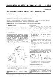
DESIGN ANALYSIS HEADING TO BETTER 

DESIGN 

Miomir JOVANOVIĆ 

Predrag MILIĆ 

Abstract: The paper describes analysis which proffing the 

success of construct design of supporting structure of pull 

railway vehicle. For this proofing type method the finite 

elements is chosen and it is used in this paper. The 

construction of model is described, criteria of quality 

control of the model and solution. The paper is program 

base of model development for similar categories of 

supporting structures. 

Key words: Structural analyse, FEM, railway vicle. 

1. INTRODUCTION 

When top quality firms develop new projects, they check 

their technical solution by asking for expert analysis with 

independent consulting firms. Those firms technically 

estimate the quality of the product. Comparing the ordered 

project with their own project, they make demanded safety 

of the design and then they achieve the quality of the 

product. Lokomotiva a.d MIN- NIŠ performed the 

Development Project of railway vehicle DHD 200 DK 

classified as diesel hydraulic dolly. The power of operating 

aggregate of the vehicle is 209 kW, capacity Q= 8 tons, 

gross mass 28 t .The vehicle is for pull service of railway 

cars and is equiped with an crane for hydraulic unloading of 

the cargo. 

This is the objective of the realization of FEM expert 

analysis, which deals with the base construction of the 

vehicle from the aspect of strenght in order of improving of 

stress-strain state of the support. The investor demanded 

quality investment technical documentation, which proves 

the design success expressed in technical measures – 

standards [6, 7]. 

The other reason of interest for the support analysis, which 

producers always have, is improvement of their own 

products. In that way, after each analysis there was 

performed the correction of structure shortages, 

rearrangement of support positions, adding or reduction of 

the mass, change of constructing joints design. 

2. CONCEPT AND ALAYSIS AIM 

Super-analysis, in this case, represents the sum of static 

structure analysis, which explores the stress of support 

continuum. The analyses were performed for 12 named 

standards situations and 5 extra combinations of external 

actions on the vehicle. The foundation of the definition of 

external influence is based on Technical conditions No. 12 

together with exploit limitations. Service pull vehicle is not 

classical locomotive because it is not for permanent pull 

function. In this sense, the extreme requests are limited by 

the project task itself since there are no adequate 

regulations. As the projector wanted to know what the 

capacity (limits of load) of the construction is, all the 

analysis according to Technical conditions No. 12 were 

performed [6]. 

The basic quality in CAD-FEA design is the development 

of numerical discrete model by which the characteristics of 

the model may be tested, torsion and flexion rigidness with 

the objective of additional adjustment of performances by 

changing of joints in structure. This is one of the additional 

targets of supper-analysis. The Chair for Transport 

Technology and Logistics of the Mechanical Faculty in Niš 

performed the described super-analysis for quality 

estimation and improvement of technical performances of 

the vehicle. 

The structure analysis was performed by the finite elements 

method, based on linear theory of deformations. The design 

is more valuable if its geometrical model is true copy. That 

is why its geometrical modeling was performed by software 

SolidWorks 2005. Discrete modeling was performed by 

FEMAP program. For algebra system of equations solving 

SSAP V.4 was used. Post processing of the design was also 

performed by FEMAP program [3]. 

Scientific aim of every analysis is the identification of 

possibilities of present available software-hardware 

resources, the maximal size of the model according to 

number of degrees of freedom and overall finite elements 

number. Additional aim of examination is the efficiency of 

application of new types of finit elements, type-tetrahedron. 

2.1. Analysis structure descriptiion 

The starting demands defined the structure as welded 

spacey frame form, made of thick sheet metal and hot rolled 

open supporters. The support carries all vehicle subsystems: 

hydraulic and pneumatic equipment, operating motor, 

power transmission, cabin, crane, loaded container, brake 

levers and cylinders, cooling system, hydraulic system for 

unloading. The support structure receives all dynamic 

forces during driving. Supporters are in the frame of the 

support structure arranged along and transversely, almost 

symmetrically [10]. Supporters are made of strong 

constructing still Fe275 group. The support is made of four 

parallel along U240 supporters, front and back frontal 

plates and several transversal opened supporters UNP200, 

UNP100, in combination with plates for enforcement of 

structure head. All elements of the support are connected by 

welding. The support dimensions are 8760x2800x1415mm. 

Pre analytic mass of the support is 4725 kg. 

2.2. Static action on the suppoprt 

Analysis in accordance to technical conditions [6] and 

Regulations V2.005 are performed according vertical, 

1

longitudinal and transversal loading of pull railway vehicle 

with the following content: 

Tab. 1. 

2 

№ Analysis characteristics: 

01 

02 

03 

04 

05 

06 

07 

8.1 

8.2 

9.1 

9.2 

10.1 

10.2 

11.1 

11.2 

Support analysis under action of vertical forces 1 Fv 

Marking criterion σper, τper, σweld, Support analyses under action of only vertical forces 

2⋅Fv (double g), Marking criterion ReH, Driving situation with several cars. 

Support analysis 1⋅Fv+ 0.75⋅Fu on bumpers. 

Marking criterion σper, τper, σweld, Front hitting with bumpers. 

Support analysis under action 1⋅Fv+1⋅Fu on bumpers 

Marking criteria of construction ReH. Pulling of the cars over pull. Support analysis under 

action 1.5⋅Fv+1.5⋅Fu on bumpers, 

Support marking criterion ReH. 

Power of pressure in automatic clutch 

Support analysis under action 1⋅Fv+2⋅Fu on automatic 

clutch, Marking criteria of construction ReH. Diagonal pressure trough bumpers 

Support analysis under action 1.5·Fv+0.5·Fu on diagonal 

bumpers, Marking criteria of construction ReH. 

Support analysis under action of inertia forces in 

length way. Static model kd·Fv+1·FIN (3g). 

Dynamic factor of vertical forces kd=1.30. Horizontal forces are inertial of all masses (M·3g) 

Marking criterion of construction ReH. Support analysis under action of inertia forces in 

length way. Static model kd·Fv+1·FIN (5g). 

Dynamic factor of vertical forces kd=1.30. 

Horizontal forces are inertial of all masses (M·5g) 

Marking criterion of construction ReH. Analysis at starting moment of the vehicle at maximal 

pull force. Static model Fv+µ·Gv 

(µ =0.33 athesion quotient,Gv vehicle weight) +Frp 

(reactive axial force in power shaft operation) 

Marking criterion of construction σper, τ per. 

Marking criterion of welding σ weld. 

Analysis of support while passing trough curve and 

side wind pressure. 

Static model kd·Fv+Fpull (pull force at speed in the 

curve) + FN (p·A, p specific wind pressure N/m 2 , A is the 

surface exposed to wind) + Fc ( centrifugal force) + FNAD 

(force because of the height of one rail in the curve)+ Fr (reactive force axial operation at pull). Dynamic factor of 

vertical forces kd=1.30. 

Marking criterion σper, τper, σweld. Check of placing pillar elevator 

Model of loading 1·MKR + 1·GKR. Two cases – position of the analysis. In the direction of 

driving and under right angle on that direction 

Marking criterion σper, τper, σweld. Support analysis at elevating (hoisting) of vehicle 

Vehicle stays at 4 positions 

Static model: From vertical forces 1·Fv. 

Two analysis: First: whole model analysis. 

Second – analysis of the connection area for elevation. 

Marking criterion σper, τ per, σ weld. 

Figure 2.1 shows the one arrangement of outer forces (case 

of vertical dynamic). Activities are worked out separately 

from all inbuilt weights, inertia forces, pull and brake forces, 

forces in bumpers (when hitting), wind forces, centrifugal 

forces, crane forces and work forces. Figure 2.2 shows the 

arrangement of masses on support with schematically shown 

rigid joints of their focuses with support. This discretely 

shown mass in points made it possible to use the same model 

for solving several dynamic tasks defined in Table 1. Figure 

2.3 shows elements of analysis 9.2 where was monitored the 

vehicle passing through curve with height H and wind of 

specific pressure w. 

2.3. Checking Criteria of Construction Strenght 

The strenght of construction still defined according EN10025 

is regulated. Static checking of tension in constant continuum 

profiled supporters was performed in standard JUS U.E7.145 

(as well as JUS U.E7.145/1). Three basic cases of loading 

were monitored with safety coefficient (ν=1.5/1.33/1.2) 

which define comparative (permitted) stresses. Permitted 

stresses refer to loading from extension, pressure and 

bending. Permitted tensions for local checking of frontal 

welding joint for typical loading cases, are defined according 

to JUS U.E7.150, by coefficient of welding strength k. Local 

checking of tension of fillet welding is performed in from 

JUS U.E7.150 and coefficient of safety ν of fillet welding 

defined according to standard JUS U.E7.081. Bends are 

empirically marked, by rigidity control: C= LMAX/YMAX. 

This is the quotient of span and elastic deflection. With still 

supporters of transport machines, the rigidity is required 

within limits of C=300÷759 (lower-upper). 

3. ANALYSIS 

3.1. Choice of Analysis Method 

The vehicle exploitation was conditioned by firmness 

checking for several characteristic combinations of static 

loadings. Obviously that quality and good construction of 

supporter comprises the ability of static endurance for 

various different influences. Classical analysis by 

deformation method of line bending supporters, with its low 

velocity and limits only on assumed critical crossing (not by 

computing procedures), do not respond to efficient design, 

because the design is achieved by many different analysis. 

That is reason because the finite elements method analysis is 

chosen. By it, numerical computing procedure was taken out 

by using only one (discrete) model for all combinations of 

loading. 

For mentioned tasks realization, the linear static FEM 

analysis was used together with program combination 

FEMAP/SSAP V.4. Construction modeling was performed 

by using the 10-node solid finite element of tetrahedron. The 

geometry was true modeled, which included the holes, 

radius, welds, extension of supporters and transitional profile 

geometry. The other important criterion is model 

development which processing was acceptable from the 

aspect of time performance of modern computer. 

For stress analysis state the comparing Von Mises tension 

and maximal tangent tension were used. The choice of 

comparative stress was performed according to stress 

category in elastic domain of support strain. The main part of 

deforming work is spent on geometry shape change, Von 

Mises hypotheses (Henky-Huber-Mises). The maximal 

comparative stresses of structure are defined by nodes in 

center of all model finite elements.

Fig.2.1. Case of forces arrangement ANALYSIS-2 

Fig.2.2 Model of mass arrangement that inertial forces come from Case of hitting vehicle in front, ANALYSIS 8.2 

3.2. Development frames of CAD-FEA models 

The condition of support developing is good understanding 

of its stress–strain state, so the type choice of finite 

elements is looked for in smaller (discrete) geometry 

domain – solids. 

Base for this is the spacey stress state of real constructions 

which is best interpreted by solids. Limits in meshing are 

conditioned by physical size of the model. The discrete 

model is looked for in range Ne=1.5.10 6 ÷2.0.10 6 of finite 

elements. This number of elements is in PC domain of 

realisation and is limited by time of numeric realization. 

The volume of average finite element (VE) is defined by 

quotient of total volume of support (defined SolidWorks 

Vp=0.6m 3 =600.000, cm 3 ) and planed number of elements: 

VE=Vp/ Ne =0,30+0,40 cm 3 . Tetrahedron of side responds 

to this volume a=2.04⋅(VE) 0.33 =1.37÷1.50 cm (size of 

element). Generated number of elements in direction of the 

support length is defined by quotient of length L=8760 and 

average size of elements geometry: NL=3⋅(585÷640). 

Number of elements in transversal direction NB comes from 

the quotient of vehicle width B=2800mm and size of 

average element a: NB=3⋅(187÷204). Number 3 is empirical 

coeficient. Out of this frame the topology of finite elements 

frame is mapped. Developed mesh describes the continuum 

up to the level of holes, roundness, ribs, and welded joints, 

the correct geometry structure. Figures 3.1 – 3.2 show the 

details of discrete model. 

Model is elastically leaned over SPRING elements by 

which the elasticity of vehicle hanging was described. The 

leanings of the support (on work wheels, bumper leaning) 

are connected with support by RIGID finite elements which 

is precisely defined model rotation. 

Concentrated masses of crane, cabin, engine, transmitions 

and loading container are linked with the construction with 

rigid elements. It enabled introduction of inertia forces by 

giving only one common vector – acceleration vector. 

3

Fig.3.1. Discrete model of the vehicle (front detail) 

Number of elements: 1.858.859. Number of nodes: 620016. 

4 

Fig.3.2. Details of the lower part – support of the crane 

4. RESULTS OF STRUCTURAL ANALYSIS 

Lets look at some of analysis results: In case of vehicle 

hitting into another one (CASE 8.2) where was 

implemented the total of outer impacts upon form: 

1.3·Fv+FH·(5g), the maximal tension was gained σVON MISES 

= 38,87 kN/cm 2 and maximal tangent tension τMAX = 20,19 

kN/cm 2 , translation: yMAX = -0.0203 m, zMAX = 0.0030 m. 

Allowed boundary stress (RE) are not exceeded RE = 41,5 

kN/cm 2 ; τE = 24,0 kN/cm 2 . The produced translations are 

within normal rigidity of construction: C = LMAX/yMAX = 

8.760/0.0203 = 431, m/m. The analysis results of the 

highest stress influenced the extreme loading zones to 

redesign. That is why area of front of support 

(forward/backward), several vertical and horizontal ribs are 

placed, figure 3.1. Such a procedure of firmness is 

implemented in all analysis, in order to eliminate places of 

material fatigue and possible damage that can come later. 

Figure 4.1-4.4 show the analysis result. 

5. CONCLUSION 

In such a way performed the group of super-analysis 

enabled to define whether the strenght of support on all 

actiones was achieved by designing. Since the number of 

request are numerous, it is sure that there will be 

corrections of initial geometry structure design. The 

corrections may be performed also in order to reduce the 

greatest equalize stresses of mass allocate of material along 

of the construction. In case when introduced criteria can not 

be fulfilled, there has to started new design. 

Fig.4.1. (Case 8-2) The maximal translation of the whole construction (mostly because of the deflection of the springs on 

the shafts) is 0.0204m. Deformations of the model are in driving direction on front bumpers.

MFN 2008 

Fig.4.2 (Case 8-2) Maximal Solid Von Mises stress (388.762.432, N/m 2 ) 

is in the area of connection of main supporters and front plate. 

Fig.4.3 (Case 8-2) Look on the lower central part of the support. 

The picture presents high fidelity of FEM model with real physical construction 

MFN 2008 

Fig.4.4 (Case 11.1) Elastic deformations ( bending) while hoisting the vehicle (factory service operation). 

The greatest deflection are in the middle 0.0165 m 

5

6 

Fig.5.1 Photography of DHD 200 DK 

Fig.5.2 Support of the vehicle DHD 200DK 

Model correction: 

Pat No: 540.02-03.01-70 

(horizontal rib on the middle vertical supporters), 

Pat No: 540.02-03.01-71 

(horizontal rib on side vertical supporters) 

During every analysis there has to be taken care of the 

quality (design) of the discrete model: Correctness of type 

choice and enough number of finite elements, quality of 

shape function At that time the greatest translations have to 

stay small and number of degenerated elements controlled. 

There may be the proof of model convergence, specially if 

there is symmetrical structure and symmetrical loading. 

Figure 5.1 shows the stage in assembly the equipment on 

support of pull railway vehicle HD 200 DK made in 

Lokomotiva a.d. MIN Nis. Figure 5.2 shows details of 

performed changes in the middle part of construction by 

which is increased the strenght of structure over diagonal 

impact. In this way defined results of group structures of 

analysis enabled to reach the decision from the design 

about new one, which make the creation of valid products. 

ACKNOWLEDGMENT 

This paper is financially supported by the Ministry of 

Science and Technological Development of Republic of 

Serbia, Project Nr. 14068. This support is gratefully 

acknowledged. 

REFERENCES 

[1] ZIENKIEWICZ O.C., The Finite Element Method in 

engineering science, McGraw-Hill, London 1971. 

[2] TIMOSHENKO S., Strength of Materials, Part II, , 

New Jersey, 1956. 

[3] MSC NASTRAN 2004, Interactive Systems, Inc, Part 

No 440.401 Supergen, Pittsburgh, 1991. 

[4] JOVANOVIĆ, M., MILIĆ, P, MIJAJLOVIĆ, D, 

Aproximate contact models of the rolling suports, Facta 

Universitatis, Series Mechanical Engineering, Niš, Vol 

2, N° 1, 2004. pp. 69 - 82, 

[5] JOVANOVIĆ, M, MARINKOVIĆ, D, Redizajn - 

optimalna geometrija nosača, COD-2002, FTN NS, 

Novi Kneževac, Maj 2002, 

[6] Technical norm №.12, Yugoslav railway union, Office 

for development and explotation, IV Rev.1978. BGD. 

[7] ŠARIĆ J., Vučena vozila, Zavod za udžbenike, 

Beograd 1996. 

[8] JOVANOVIĆ, M, MILIĆ, P, Enhancing tehnology of 

geometry shape container design, ADEKO FTN Novi 

Sad, Machine design., 2007, pp. 89-92. 

[9] JOVANOVIĆ, M, JANOSEVIĆ, D, MILIĆ, P, 

Structural CAE Identification of Boundary Loads of 

Excavators, International Conference Interstroimech 

2004, Voronez, Russia, 2004. 

[10] JOVANOVIĆ, M, KΟΖΙĆ, P, MILIĆ, P, Structural 

analysis of railway vehicle support DHD 200 DK- 

Lokomotiva a.d. MIN Niš, Development Project No. 

612-22-168-2/08, Final Raport, Mechanical Faculty of 

Niš, 2008. 

CORRESPONDENCE 

Miomir JOVANOVIĆ, Prof. D.Sc. Eng. 

University of Niš 

Faculty of Mechnical Engineering 

Chair of Transport tec. and Logistics 

Str. A. Medvedeva 14 

18000 Niš, Serbia 

miomir@masfak.ni.ac.rs 

Predrag MILIĆ, B.Sc. Eng. 


Faculty of Mechnical Engineering 

Chair of Transport tec. and Logistics 

Str. A. Medvedeva 14 


pmilic@masfak.ni.ac.rs

DESIGN METHODOLOGY OF 

AUTOMATED DISASSEMBLY DEVICE 

Radovan ZVOLENSKY 

Karol VELISEK 

Peter KOSTAL 

Abstract: Disassembly is new and also rapid developed 

trend in the manufacturing area. In the future the 

disassembly will be inseparable part of manufacturing 

process. Especially this fact will be important for that 

part of industry, which is focused to the products with 

variable nature. The nature of such variable products is 

changing following to the customer requests. Especially 

automated disassembly is an technology, which is 

attempting to satisfy such needs and requirements. Many 

of such special requirements are supported by 

international institutions, research programs and 

foundations. Automated disassembly technique allows 

automated separation of various parts, from which was 

disassembled product created. 

Keywords: Disassembly, Robot, Flexible 


Creation and design of automated disassembly device is 

an complex problem, which includes design problematic 

of automated device. Of course automated device design 

problematic is consequently adjusted following to the 

requirements of disassembly devices design problematic. 

Such designing process, which is designing automated 

disassembly device needs some guide. This guide will 

carry designer over the all problems which are connected 

with disassembly process and also its automation. After 

using of such guide, some automated disassembly device 

will be designed. Such guide, or better say such tool is 

and methodology of automated disassembly devices 

design. 

2. METHODOLOGY OF AUTOMATED 

DISASSEMBLY DEVICE DESIGN 

Each automated device consists of several building units 

such as suspension frame, manipulating equipment, 

working equipment, helping equipment, or control 

equipment. The same building units have to be designed 

and created by design of automated disassembly device. 

Of course choose of these building units will be limited 

by activities realized by disassembly processes. There is 

also very important to realize analysis of disassembled 

product before design of automated disassembly device. 

All information getting from this disassembled product 

analysis can be used for creation of proper disassembly 

method. In the first phase of disassembly method creation 

is important to focus on all movements which are realized 

during disassembly process. This way created 

disassembly method has to be supplemented by other 

information. With help of these information, there will be 

possible to create internal structure of disassembly 

method, or other alternatives of whole disassembly 

process. Ending of first analytical phase, which is used for 

disassembly method creation, is creation of disassembly 

method in form of disassembly combine processual 

diagram. 

In the other phase is methodology for design of automated 

disassembly device dealing about the choose of proper 

automation instruments. This choose is realized regarding 

to the created disassembly method and also regarding to 

the techniques of assembly joints destruction. Following 

to the choose of proper automation instrument, there is 

needed other one choose of building components of whole 

automated device. These building components are for 

example power unit, signal unit, control unit, or carrying 

unit which is generating frame of whole automated 

device. 

Last activity, which is really important for creating 

process of whole device is choose of proper control 

system. This choose is partially given by kind of chosen 

automated instrument. This activity is also that one, which 

creates single steps of control, or whole control method. 

Whole control method really close follows disassembly 

method, which was created in analytical part of design 

methodology. 

2.1. Disassembled product analysis 

Input of most manufacturing of assembly technologies is 

analysis of manufactured or assembled product. This 

analysis is analyzing product from many views. Also 

design of disassembly device needs product analysis, 

which will look to the product from many valuation 

views. The number of valuation views can be different, 

usually the number depends on complexity or largeness of 

whole disassembled block. Valuation views which are 

valuated disassembled product can be divided in the five 

groups. 

� Disassembled element analysis according to the 

recycling kinds of single building products, 

� Disassembled elements analysis according to its 

influence to the environment, 

� Disassembled elements analysis according to the 

design materials of disassembled products, 

� Disassembled elements analysis according to the using 

assembly joints or according to the used assembly 

technologies, 

� Dimension and shape analysis of single products, 

which are used during the whole assembly process. 

7

Information which comes from these analyses are then 

used for identification of parameters which are limiting 

the following disassembly process. 

2.2. Disassembly process design 

For proper disassembly process design is necessary to 

know, the process which was used by its assembly. 

8 

Fig.1. Assembly process of pneumatic actuator 

From that reason we use, as an input for disassembly 

process design, assembly processes and other assembly 

documentation. If such information and materials are not 

available it is necessary to create own input data. The tool 

which can be used for such input data creation is for 

example step diagram, which is added by information 

taken from assembly product joints analysis. 

Fig.2. Step diagram for assembly of pneumatic actuator 

This way created assembly process can be later reworked 

by process of creating of reverse step diagram. In case of 

more complicated design, not only reverse step diagram 

can be used. This solution needs, because of complicated 

and large design, the creation of internal structure, which 

will simple whole this kind created diagram. 

Fig.3. Reverse step diagram 

Diagram doesn't includes logical branching and 

conditions, which are needed for effective disassembly 

process. From this reason the reversed step diagram have 

to be supplemented by conditions and rules, which are 

presented by Petri net theory. 

Fig.4. Supplemented step diagram 

This way created diagram is an combination of two kinds 

of disassembly process designs. This way created scheme 

offers more information which can be used for design of 

automated disassembly device. Using of logical functions 

is necessary. This way created diagram also deals about 

need of sensors equipment, which will be used for

ealization of disassembly device. On the other hand this 

scheme also shows basic movements which are needed 

for whole disassembly process and its also shows need of 

movement actuators which will be needed for realization 

of whole disassembly device. Diagram of this type was 

specially designed and created for needs of automated 

disassembly devices design methodology and is also 

combined by automated devices design problematic. 

Diagram in this version can be used for whole 

disassembly process description. It is also very important 

guide for design of whole disassembly device. From this 

reason, the creation of such simple and tabular diagram is 

very important step in the process of automated 

disassembly device design methodology. 

3. AUTOMATED DISASSEMBLY DEVICE 

DESIGN 

Methodology solves the automated disassembly device 

design in several levels, which are influencing one to 

another. First two solution levels are the design of 

elements which are creating the working space of whole 

device and design of disassembly device manipulation 

device. Both these problematic has also mutual 

relationship. As first one the problematic of working 

space is solved. This problematic deals about the number 

and also the character of manipulating and working 

places. Inputs, which are needed for this problematic are 

reversed disassembly step diagram, which was presented 

in the last chapters. 

Fig.5. Automated disassembly device design 

methodology 1/2 

The output of workspace elements design is and creation 

of first working space picture. Such working space picture 

or first alternative design is an elements which strongly 

influence to the following methodology chapter - design 

of manipulating part of disassembly device. Working 

space picture is an connection between the design of 

manipulating part and working part of disassembly 

device. Design process of manipulating device deals 

about design of power unit, design of clamping units, 

design process of clamping jaws. During the design 

process of manipulating unit, it is very important to focus 

on parameters such as load, dimensions, power, 

performance, manipulating repieability, clamping 

dimensions and so on. For definition of these parameters 

the methodology uses external inputs in the form of input 

analysis or step diagrams. 

Information which are coming from these starting 

activities realized during the methodology using are also 

input data for other two activities. The realization of these 

two activities is important for design of the automated 

disassembly device. 

Better say the activities such as working space character 

and manipulating device will have influence to the design 

of main frame and to the control unit design of automated 

disassembly device. On the opposite side, the activities 

such as main frame design and control unit design are not 

influence one to another. But it is better to solve main 

frame design as first one, because the design of whole 

device will be that realized by more simple way. The end 

of whole automated disassembly device design process is 

characterized by activity called collision analysis. This 

analysis defines single zones created in the working space 

of the device such as manipulating zone, working zone, 

non usable zone, and so on. This activity defines the 

intersections of these zones and analyses possible 

collision stays. 

Fig.6. Automated disassembly device design 

methodology 2/2 

The next one activity which is realized in the design 

methodology is design of control unit. This activity 

includes the design of control elements, design of 

processing elements, design of storage elements, design 

of control elements and design of signal elements. Main 

area of this activity is focused on the design of control 

algorithm of automated disassembly device, which will be 

realized in three steps. These steps are creating of step 

diagram, creating of progress table and creating of 

normalized tool called Grafcet. With connection of these 

three parts the design of whole automated disassembly 

device is can be realized. 

9

4. CONCLUSION 

Designed methodology, step by step deals about single 

activities and works. Realization of such activities is 

necessary for complex design of automated disassembly 

device. Single steps are using known analytical project 

methods which are modified following to the disassembly 

devices problematic. But generally the methodology of 

automated disassembly device design stand on the 

methods which were specially created for needs of 

disassembly devices needs. Methodology includes before 

project as well as project phases, which are followed by 

design phases of whole automated disassembly device. By 

connecting of updated well known methods and 

specialized newly created methods a new methodology is 

created, and it is able to create working automated 

disassembly device. 

REFERENCES 

[1] ZVOLENSKÝ, R., RUŽAROVSKÝ, R., KOSTÁĽ, 

P: Design of automated disassembly devices, 

MicroCAD 2008, ISBN 978-963-661-812-4, ISBN 

978-963-661-822-3, pp 51-56 

[2] ZVOLENSKÝ, R., RUŽAROVSKÝ, R., VELISEK, 

K: Design of automated manufacturing and 

disassembly systems, Machine Design 2008, Novi 

Sad, ISBN 978-86-7892-105-6., pp. 277-282 

10 

[3] ZVOLENSKÝ, R., RUŽAROVSKÝ, R.,: Design of 

automated disassembly devices, Education Quality - 

2008, ISBN 978-5-7526-0355-6., pp. 122-126 

[4] ZVOLENSKÝ, R., RUŽAROVSKÝ, R., : 

Technological devices of flexible manufacturing cell. 

, Education Quality - 2008, ISBN 978-5-7526- 

03556., pp. 194-200 

[5] JAVOROVÁ, A., ZVOLENSKÝ, R., PECHÁČEK, 

F., VELÍŠEK, K.: Computer aided design of 

automated assembly system, Archiwum technologii 

maszyn i automatyzacji - 2008, ISSN 1233-9709. 

pp. 139-147 

[6] MATÚŠOVÁ, M., JAVOROVÁ, A.,: Modular 

clamping fixtures design for unrotary workpieces, 

Annals of Faculty of Engineering Hunedoara - 

Journal of Engineering 2008, ISSN 1584-2673, 

pp. 128-130 

[7] MATÚŠOVÁ, M., HRUŠKOVÁ, E.: Simulation of 

machining in CATIA V5R15. KOD 2008. ISBN 978- 

86-7892-104-9, pp. 71-72 

[8] Charbulová, Marcela - Mudriková, Andrea: Fixture 

devices with modular conception. In: AMO 2008: 8th 

international conference on advanced manufacturing 

operations. Bulgaria, Kranevo, 18-20 June 2008. - 

Sofia : DMT Product, 2008. - S. 123-126 

[9] Mudriková, Andrea - Hrušková, Erika - Horváth, 

Štefan: Model of flexible manufacturing - assembly 

cell. In: RaDMI 2008 : 8th International Conference 

from 14-17.September 2008, Užice. - , 2008. - A-27 


Radovan ZVOLENSKÝ, Ing., PhD. 

Slovak University of Technology 

Faculty of Material Science and 

Technology, Department of 

manufacturing devices and applied 

mechanics, Rázusova 2 

917 24 Trnava, Slovakia 

Radovan.zvolensky@stuba.sk 

Karol VELÍŠEK, prof., Ing., Csc. 







Karol.velisek@stuba.sk 

Peter KOŠŤÁL, doc., Ing., PhD. 







Peter.kostal@stuba.sk

AN APPROACH TO MECHATRONIC 

SYSTEM DESIGN PROCESS – THE ON- 

LINE ENGINEERING OFFICE 

Gorazd HLEBANJA 

Abstract: The basic characteristic of emerging production 

and design systems is their “atomisation”. The role 

of the innovative design in economic growth of companies 

is crucial. And a distributed development environment 

must develop a new working paradigm, adapted to new 

sophisticated requirements. Thus, an adaptive, competent 

network structured design system based on the virtual 

coordination unit (VCU), facilitating innovative high tech 

product or mechatronic system design, had been developed 

[1,2]. A concept of the on-line engineering office in 

assistance of small and medium sized enterprises (SME) 

is developed and elements of such internet based service, 

basic and specialised tools and methods are stressed in 

this paper. 

Key words: Distributed development environment; Virtual 

coordination unit; Virtual competence centre; On-line 

engineering office. 


Problem discussed in this paper is related to high tech 

product design and development in small and medium size 

enterprises (SME), which have only limited resources to 

develop such products. However, their market position and 

competitiveness strongly depend on new innovative, creative 

goods, which basically consist of a mechanical structure, 

electronic and micro-processing devices, as well as 

programs or even intelligent software for the implementation 

of the operations control. This means that the complexity 

of the HT-product development, design and manufacturing 

requires a number of highly competent and knowledgeable 

subjects in different fields. It also implies usage of the 

newest methods, tools, and variety of data and knowledge 

bases. At last, results of fundamental and applied research 

are indispensable in development of new artefacts. On the 

other hand, SMEs are performing excellently in their specialised 

domain. To become and remain in such state they 

should optimise their development and work systems to 

their production. Problems are lack of knowledge, experi- 

ence and man-power in other fields, e.g. development of 

promising new products or systems, technologies, factory 

automation, etc. Thus, questions raised here from the SMEs 

viewpoint are 1) about definition of a new product itself 

and its production technology and 2) search for competent 

developers and developing tools. 

Yet another aspect in engineering design is that designers 

are dealing with uncertainty starting from inexact specifications 

and only the degree of their competence makes 

possible convergence towards an improvement or new 

product. It is necessary to gain new information, to decide 

upon and build a model and possibly incorporate this in a 

particular design. This could be regarded as innovation 

process. Only LMC are capable of continuous innovation. 

A high tech product or mechatronic system design requires 

methods, tools and expertise in several engineering 

fields, thus project based organisation of development is 

evident. In this context collective competence should be 

defined, composed of all individual knowledge and experience, 

necessary to successfully implement a task. 

Variety of tools, methods and “over-informed” staff make 

recognition of good design choices more difficult and 

again competence is of vital importance. 

Therefore, a new design and development paradigm, suitable 

for growing market demands and coping increasing 

product and system complexity, should be established. 

Such an innovative design and development D&D structure 

has been reported upon in detail [1, 2] and is resumed here 

briefly. The D&D process thus starts from a product specification 

proceeds through the innovative development and 

design, prototype and manufacturing technology elaboration 

to a working prototype. Both processes, namely design 

and prototyping are conducted by specialised engineering 

teams. Since collected engineering knowledge might be 

insufficient, additional training should be available. In order 

to access additional less focused, broader knowledge on 

design and technology applied and manufacturing research 

teams are employed. Efficient cooperation of all teams and 

individuals collaborating in product formation is of crucial 

importance. In this context a virtual coordination unit 

(VCU) was developed [1]. 

The basic tasks of the VCU are a) organisation and management 

of the data stored in various data and knowledge 

bases, on different locations; b) maintenance of effective 

communication, coordination and control of the activities 

performed by the subjects of various teams and the teams 

as a whole; c) communication with the innovation management, 

reporting on every significant aspect in the development 

and design of the HT-product; various aspects 

of patent management; d) organisation of additional training 

courses on-line for the subjects working in development 

and design prototyping teams; e) survey of the research 

activities of various research teams at universities, 

research institutes, companies: manufacturing capacities 

of the SME participating in the production of HTproducts: 

etc. 

The VCU-function of coordination and control includes a 

fast and reliable communication with the manager, various 

teams and team subjects, the researchers of the in-and 

outside the R-units, the training bodies, patent office etc. 

The IT with the Internet and LAN-structures are the most 

capable means for realization of the virtual coordination 

function. 

11

Whereas the coordination of processes is performed by 

the virtual coordination unit (VCU), a virtual competence 

centre (VCC) has been introduced for communication, 

teamwork and cooperation support [3]. It provides communication 

among team members, teams and VCU. The 

communication is carried out over the VCC portal. The 

portal enables access to data and knowledge bases, applications 

and web services that are intended for common 

usage. The portal also provides a common electronic 

work-space in order to support communication and asynchronous 

cooperation. 

Contemporary information and communication technologies 

(ICT) enable different means and methods for ecollaboration. 

The key requirements for implementation 

of the D&D collaboration framework are functional and 

resource integration; synchronous and asynchronous 

communication; data, file and document management; 

project management; and common cooperation space in a 

distributed environment. Besides, the ICT platform has to 

assure a high level of privacy, safety, and reliability. 

2. ON-LINE ENGINEERING OFFICE 

As market circumstances – i.e. growing product complexity 

and functionality, less predictable market, demands on 

higher quality, etc., – influence production companies, 

this reflects design and development as well. So as companies 

develop organizational forms enabling prompt 

adaptation and much higher flexibility, similar transformation 

is necessary in design and development domain. 

Goals of such an adaptation should be faster response, 

flexibility, ability to collaborate in a distributed environment, 

mastering increased complexity, cross-domain col- 

12 

DB 

DATA 

PROCESSING 

KB 

RB 

INTERNET 

VCU - Virtual coordination unit 

D&D + PMT 

D&D + ART 

DATA AND 

KNOWLEDGE 

BASES 

DATA 

PROCESSING 

PMT + MRT 

PROCESS 

IMPLEMENTATION 

DEVICE 

RB 

Prepared 

data and 

knowledge 

Fig.1. Virtual coordination unit structure [1] 

DB 

DB 

laboration, mastering information flow, improving mutual 

communication to avoid misunderstandings. D&D tasks 

in such environment are becoming more complex and 

more diverging in general; time spans to accomplish such 

tasks are narrowing. 

This also essentially influences organizational structure. 

In the paper proposed formation uses an adaptable ad/hoc 

networked development environment collecting: 

� human expertise, 

� engineering tools, 

� web tools and methods, 

� data and knowledge bases, and 

� communication and collaboration tools. 

E.g. human expertise is valuable, however, it is very often 

hidden, it is difficult to discover information even if 

someone would have paid for it and previously stated 

environment makes it available. Thus, such an environment, 

collecting tools and human knowledge and coordination 

through internet enables better design and development 

possibilities also for SME. 

Fig. 2 reveals the structure of the proposed on-line engineering 

office (OLEO) [16]. The OLEO environment 

backbone is a VCC portal assuring access to its particular 

elements [19]. Experts, competent professionals, use engineering 

tools on everyday basis. They also use data 

bases needed in design process, e.g. TraceParts [4]. 

Communication and collaboration tools in OLEO are of 

crucial importance. Rules regarding special design features 

(Die casting, molding, etc.) could be to some extent 

part of engineering tools (integrated in CAD systems), 

however many special methods and knowledge are systemized 

in additional tools, services or knowledge bases. 

Through internet accessible are supplementary, even 

PB 

Legend: 

DB - DATA BASE 

PB - PRODUCT BASE 

RB - RESEARCH BASE 

KB - KNOWLEDGE BASE 

D&D - Development & design team 

ART - Applied research team 

PMT - Prototype team 

MRT - Manufacturing research team

SME1 

SMEx 

WORK 

SYSTEM1 

ENGINEERING OFFICE 

KNOWLEDGE 

BASES 

Design, planning, 

manufacturing rules 

Algorithms 

Decission trees 

Associative rules 

... 

DATA 

BASES 

competing or complementary tools, services and methods, 

as well work systems implementing prototypes and even 

labs, when experimental research is needed. 

Production SMEs are in the position of customers, they 

require information, service or finished design. In this 

KNOWLEDGE 

BASE1 

SERVICES 

AND METHODS1 

PARTS , 

ME CHANICAL 

ELEMENTS, 

TECHNOLOGY, 

... 

METHODS 

AND/OR 

SERVICES 

ENGINEERING 

TOOLS 

SME2 

Tolerancing, 

Design specialties 

(Die casting, molding, 

... ready design) 

CAD 

CAPP 

CAM 

FABRICATION 

LABORATORY1 

ENGINEERING 

OFFICE 

ENVIRONMENT 

COMMUNICATION 

COLABORATION 

TOOLS 

PART 

DATA BASE1 

PDM 

DATA EXCHANGE 

Viewers 

ENGINEERING 

OFFICEo1 

Fig.2. On-line engineering office structure 

INQIRIES 

SPECIFICATIONS 

EXPERT 

EXPERT 

EXPERT 

VCC PORTAL 

DELIVERED 

CONTENTS 

ENGINEERING 

OFFICEi1 

context the OLEO could be regarded as a special type 

ADMS (adaptive distributed manufacturing system), 

where a design is in the role of a product. 

An accomplished project could even result in mutual efforts 

of several OLEO, which could be in a long term 

SERVICESn 

VIRTUAL COORDINATION UNIT - VCU 

SMEn 

13

cooperation or in an ad-hoc connection, some task could 

be outsourced. The ability of an ad-hoc grouping in a case 

of necessity is advantageous. However, this is true only, if 

collected knowledge and experience (i.e. competence) and 

design process coordination lead to the objective to be 

accomplished. 

The OLEO is therefore characterized as a web based online 

accessible engineering facility with sufficient competence 

and abilities in at least one main engineering development 

and design area and ability to form or adjoin another 

corresponding facilities based on their and collected 

competence. Functionalities then depend on design and 

development tasks that the OLEO is competent in. 

2.1. Tools 

High-tech or mechatronic systems – innovative products 

in general –development and design require interdisciplinary 

combination of mechanical, electronic, control and 

information engineering development in a concurrent 

manner, so called cross-domain engineering to build the 

underlying mechanical and electrical structure, and its 

control and programming environment to accomplish the 

system integration. Traditional engineering sequences 

could not result in an optimal solution. 

Innovation lies prevailing in early design phases, regardless 

of the design methodology in use, structured [5,6] or axiomatic 

design [7], which are basically not fundamentally 

different [8]. It appears that VDI systematics [6] helps to 

position tools and methods used in product development in 

a particular spot. Several interacting sub-models should be 

developed during HT product design already in the principal 

solution phase: a) demands, b) environment, c) target 

system, d) working structure, e) shape, f) functions, g) scenarios, 

h) working characteristics (e.g. dynamic response, 

digital logic, etc.) [9]. Table 1 contains characteristic examples 

of tools used in the OLEO. 

2.2. Communication, collaboration and coordination 

Communication, collaboration and coordination are essential 

in an efficient OLEO: 

1. communication between engineering office and customer, 

i.e. SME, 

2. collaboration among developers, regardless it is intra- 

or inter-offices or customers, 

3. coordination of development and design project. 

Means of communication could be categorized in 

� asynchronous tools (e.g. mailers, task organizers, file 

exchange, etc.), 

� videoconferencing, web dialogs (e.g. Unyte), 

� model visualization tools, 

� tools enabling collaborative functional use of a CAD 

system, 

� project oriented collaboration using PDM systems 

Collaborative engineering is facing several problems, 

namely: lack of collaboration tools integration, incompatibility 

of tools, ad-hoc collaboration, failing standards, 

data security, etc. 

2.3. Services 

Complex design and development tasks are usually effectively 

conducted in a collaborative environment, governing 

14 

by a PDM system. However, this is not true for more specialized 

methods, which might even not be feasible for 

computerization or implementation on the web. On the 

other hand many particular methods are web accessible and 

could provide an important improvement in the OLEO. 

E.g. special gearing [17,18] design methods could have 

been organized in this way. Thus it is necessary to develop 

1) an evaluation procedure to facilitate selection in the web 

plenitude, and 2) a means of access in an OLEO. Methods 

of this type should be organized as services. 

Table 1. Tools of the OLEO 

Mechanical develop- FEM, mechanical 3D modelling, assemment 

tools 

bly, mechanical simulations, drafting, … 

Specialised tools sheet-metal development, moulding, …, 

pipelines, .. 

Electronic develop- Orcad, Eagle 

ment tools 

Control system model- Simulink/ Matlab, Matrixx/SystemBuild 

ling tools 

System simulation Modelica/Dymola 

Software development programming languages C++, C#, Java 

tools 

µprocessor libraries 

Common services Data exchange protocols (STEP, VDA, 

IGES, SET, …, xml, …) 

System modelling UML, Fujaba, … 

Methods Machine part calculations, special calculations 

(e.g. non-involute gears, CMM 

ready tolerancing, … 

Data bases Proprietary parts, WEB data bases (TraceParts, 

…) 

Knowledge bases Design rules, manufacturing/assembly 

ready design, … 

Collaboration tools Smarteam, WindChill, … 

Service is an activity that the service provider offers to the 

service receiver in a service environment and generates 

values for the service receivers [10]. 

INQUIRY 

SERVICE 

REQUEST 

SERVICE 

REGISTRY 

BIND 

SERVICE 

DESCRIPTION 

PUBLISH 

SERVICE 

PROVIDER 

Fig. 3. Service search engine 

SERVICE 

SERVICE 

DESCRIPTION 

Web services base on Service-Oriented Architecture 

(SOA). This concept is based on an architectural style that 

defines an interaction model between three primary parties: 

the service provider, who publishes a service description 

and provides the implementation for the service, a service 

consumer (receiver), who can either use the uniform resource 

identifier (URI) for the service description directly 

or can find the service description in a service registry and 

bind and invoke the service, Fig. 3. The service broker provides 

and maintains the service registry [11]. The registry

in a network community is in principle public However, it 

should be kept in a domain of the OLEO in this case. 

3. DESIGN SCENARIO 

A design scenario is employed as an illustration of the 

OLEO concept, in this case an automated testing rig for 

observation of slow speed rolling sliding contacts, developed 

at the Faculty of Mechanical Engineering in Ljubljana 

[12]. Many heavy duty machines, final stages of 

power transmissions, etc. incorporate such contacts, 

which are particular in their properties, damage forms, 

etc. Experimental work contributes to the development of 

a useful contact model of such processes, thus improving 

design of such contacts. 

Normally the D&D process would have been started with 

the market research, affirming state of the art, market 

needs and perspectives, continues with specification, in 

depth iterative (system) development, and a working prototype 

development (system integration) [1,2], which also 

includes product testing, its acceptance and certification 

(if feasible). Manufacturing technology, assembly and 

quality control considerations would be also required in 

case of anticipated serial production [14]. 

In this particular case an equivalent to the HT product 

specification process [1] was necessary. The scientific 

research on feasibility and industrial relevance of such 

experimentation and its results had to be conducted in the 

first place. Upon acquired information some decisions 

could be derived. 

The consequent pre-project phase aims a) to define a task 

specification, and b) to form a D&D team in which a mechanical 

designer, electronic engineer and a scientist contribute. 

The situation analysis should answer questions 

regarding experimental conditions. In this early development 

stage, several aspects, influences and preliminary 

sub-models should be worked out. These include envi- 

Osciloskope 

Plotter 

Adjustable switch-off 

electronics 

C 

to M/N 

Counterweight 

Strain-gage beam 

transducer 

Carrier amplifier 

A/B 

C 

D E 

I. 

II. 

Counting card 

Velocity program 

NI Lab PC+ card 

Friction force 

Shocks 

Shifting 

Surface profile Microscope Balance 

I 

I 

ronmental conditions and influences, experimental strategies 

(scenarios) elaboration, definition of functional structure 

and functional units, working structure elaboration, 

and preliminary shaping [13]. 

The above analysis implied a testing rig boundary conditions, 

that is cylindrical convex-convex rolling-sliding 

contact, speed range according to Stribeck’s curve between 

0,035 and 0,2 m/s, Hertzian pressure up to 1400 

N/mm 2 , experiment duration up to 500 hours (fatigue cycles), 

sliding circumstances, etc. Consequently, the machine 

size can be defined, i.e. normal force up to 10000 

N. Several aspects were considered afterwards, e.g. long 

term experiment stability, assurance of automatic and 

punctual stop in case of damage (scuffing), etc. The result 

in this phase was redefinition of demands, confirmation of 

a functional model, experimental scenarios elaboration, 

etc. Based on above, a so called “semi-operational” 

scheme was developed, Fig. 4. Based on the pre-project 

information review and evaluation of expenses it was 

decided to proceed with the project. 

The mechanical structure was produced and assembled in 

an external facility and the machine integration, revival 

and testing took part prior to final delivery. 

The testing rig made possible slow speed rolling-sliding 

contact experiments, thus enabling research on cold scuffing, 

wear and pitting phenomena. 

The testing rig was developed using computer tools. Experiments 

have been controlled and monitored by computer. 

However, the development environment was not 

integrated to the extent prevailing today, communication 

being physical, by phone or by e-mail and file based. 

How could an OLEO benefit to the above project? 

� First of all there is the necessity of an integrated development 

environment, which enables better coordination, 

on-line accessible data, easier communication, 

…; 

� the role of the VCU [1]; 

Timer 

i 

i 

NI LABVIEW 

DOCUMENTATION, 

EVALUATION, 

ANALYSES 

COMPUTER 

Planetary gear train Frequency inverter 

A/B 

M 

Motor 380V 

M 

Incremental 

transducer 

with electronics 

M/N 

Fig.4. Virtual coordination unit structure [1] 

Files 

Amplifier 

LVDT 

Weights 

E 

signal Charge Amplifier 

Shock 

D 

15

� using video-conferencing and visualisation tools for 

brainstorming, clarifying technical details; 

� less or no transportation time and expenses, better 

prepared meetings; 

� particular specialists enter D&D process only and if 

necessary for the time needed to accomplish their task; 

� efficient project management; 

� better efficiency in general. 

4. CONCLUSION 

The need to restructure basic characteristics of emerging 

production and design systems was exposed in the paper. 

The concept of the adaptable and competent network 

structures for D&D process innovation has been resumed 

and the role of the virtual coordination unit exposed. Furthermore, 

an on-line engineering office (OLEO) structure 

has been proposed in order to facilitate distributed development 

of innovative high tech products and mechatronic 

systems also for SME. The structure of OLEO has been 

explored with regard to necessary human expertise, engineering 

tools, web tools and methods, data and knowledge 

bases, and communication and collaboration tools. 

Through the illustrative D&D scenario importance of web 

based integration was pointed out. 

However, at present time this task appears to be of extreme 

complexity. Therefore the aim should be narrowing 

the OLEO domain to a controllable extent. Furthermore, 

methods capable of implementation as web service should 

be defined and evaluated, to gain their competence in the 

OLEO domain. 

And finally it should be stated, that an OLEO is a step 

towards a flexible flat organization, where each partner 

contributes according to his expertise. Thus, in case of 

complex project, many contributing partners can combine 

their competences in order to accomplish their goal. In 

comparison to research and design departments there is no 

need to continually assemble an organized form. 

And tools enabling such virtual enterprises – virtual portals 

are becoming more and more sophisticated each day. 

Activities like interpreting and proofreading can already 

fully rely in virtual platforms. Importance and potential of 

such “virtual” organization has also been widely recognized 

in several European FP6 projects, e.g. VRL KCiP 

(Virtual Research Lab for Knowledge Community in Production), 

which recently transformed in Emiracle [15]. 

REFERENCES 

[1] PEKLENIK, J. (2004). Adaptive and Competent Network 

Structures for the Development and Design of 

High-tech Products. In Tichkiewitch, S. (Ed.), Brissaud, 

D. (Ed.). Methods and Tools for Co-operative 

and Integrated Design, p. 183-194. Kluwer. 

[2] PEKLENIK, J. (2006). Adaptable Network Manufacturing 

System – ANMS, A New Paradigm for Structuring 

of an Innovative Industrial Production. In 39 th 

CIRP ISMS; June 7-9, p.9-16, Univ. of Ljubljana. 

[3] SLUGA, A., BUTALA, P., PEKLENIK J. (2005). A 

Conceptual Framework for Collaborative Design and 

Operations of Manufacturing Work Systems. Annals 

of the CIRP, 54(1):437-440 

[4] www/traceparts/com 

16 

[5] PAHL, G., BEITZ, W. (1996). Engineering Design; 

A Systematic Approach, 2 nd ed. Translated by Wallace 

K. Springer, London. 

[6] Design methodology for mechatronic systems. VDI 

Richtil.-2206 (2004) 

[7] SUH, N.P. (2001). Axiomatic Design, Advances and 

Applications. Oxford University Press, Oxford. 

[8] MEIJER, B. R. (2006). Self Organization in Design, 

In: ElMaraghy, H.A., ElMaraghy, W.H. (Eds.). Advances 

in Design. Springer, London, p.49-59. 

[9] Innovationspotenziale in der Produktentwicklung. 

KRAUSE, F.-L., FRANKE, H.-J., GAUSEMEIER, 

J., (Eds.), Hanser, Muenchen (2007). 

[10] TOMIYAMA, T., SHIMOMURA, M., WATANA- 

BE, K., (2004). Proceedings of DETC’ 04, ASME 

2004 Design Engineering Technical Conferences and 

Computer and Information in Engineering Conference, 

28.9-2.10 2004, Salt Lake City. 

[11] ARSANJANI, A. (2004), Service-oriented modeling 

and architecture, http://www.ibm.com/developerworks/ 

library/ws-soa-design1/ 

[12] HLEBANJA, G., PEKLENIK, J. (2003). Characterization 

of slow rolling-sliding contact process. CIRP j. 

manuf. syst. Vol. 32, No.5, p.357-366. 

[13] GAUSEMEIER, J., FRANK, U., SCHULZ, B. 

(2005). Domänenübergreifende Spezifikation der 

Prinziplösung selbstoptimierender Systeme. In: 

Mechatronik 2005 - Innovative Produktentwicklung, 

VDI-Berichte, Nr. 1892.1, VDI Düsseldorf. 

[14] ISERMAN, R. (2008). Mechatronische Systeme. 2. 

volst. neu bearb. Auflage. Springer, Berlin, Heidelberg. 

[15] http://www.vrl-kcip.org/spip.php?page=sommaire 

[16] HLEBANJA, G., PEKLENIK, J., MITROUCHEV, P., 

SLUGA, A., BUTALA, P. (2008) The virtual research 

lab for a knowledge community in production, Deliverable 

No. D27-48 on new working methods for 

knowledge and communication management, for the 

support of designers and engineers in design synthesis: 

VRL-KCiP-WP No. 3: JRA-WP3. Ljubljana: Faculty of 

Mech. Eng.; FP6 Prog., 2008. 25 p. 

[17] HLEBANJA, G., HLEBANJA, J., ČARMAN, M. 

(2009). Cylindrical wormgearings with progressively 

curved shape of teeth flanks. Stroj. vestn., 2009, vol. 

55, no. 1, p. 5-14, 

[18] HLEBANJA, J., HLEBANJA, G. (2005). 

Anwendbarkeit der S-Verzahnung im Getriebebau : 

Nichtevolventische Verzahnungen weiterentwickelt. 

Antriebstechnik (Mainz, 1982), vol.44, No.2, p. 34-38. 

[19] HLEBANJA, G., PEKLENIK, J., SLUGA, A. (2008). 

The role of the virtual coordination unit in design 

process - on-line engineering office. Conf. on Knowledge 

Management in Product Development, University 

of Twente, The Netherlands, April 9-11, 26 p. 


Dr. Gorazd Hlebanja 

University of Ljubljana 

Faculty of Mechanical Engineering 

Aškerčeva 6 

1000 Ljubljana, Slovenia 

gorazd.hlebanja@fs.uni-lj.si

MACHINING FIXTURE DESIGN VIA 

EXPERT SYSTEM 

Djordje VUKELIC 

Janko HODOLIC 

Abstract: This paper presents development of an expert 

system for machining fixture design. System provides new 

fixture construction design for specified input parameters 

on basis of adequate production guidelines. Paper 

provides applied methodology basic structure, specific 

systems segments review, and example of systems 

implementation in industrial production. In closing, there 

are conclusions, developed systems advantages and 

disadvantages, and directions for future research. 

Key words fixture, design, expert system 


Many important results are made by research in field of 

artificial intelligence for past two decades. Ones of the 

most significant are development and application of 

programs known as expert systems. Nowadays, these 

systems are research subject in specific part of artificial 

intelligence and in computer technology generally, 

referred as knowledge engineering. Expert systems are 

„inteligent“ programs which have bulit in large amount of 

highquality knowledge from some part of human 

activities, and they can process that knowledge in couse 

of sucessfull solution of a specific problem on more 

intelegent manner then human. Expert systems mainly 

manipulate with symbol token data and they do not work 

with previously determined algorithms, or with 

algorithms in classical meaning. Non-algorithm approach 

is one of the basic attribute of expert systems. Expert 

systems provide conclusions that do not have to be right 

or wrong, they can be more or less possible or reliable. 

Problems that can be solved by using of expert system are 

often poorly structured, so they are mathematically 

modeled and formalized. This means that standard 

algorithm approach is practically inapplicable in solving 

these problems. Algorithms and data are defined by 

classical programming principles. Algorithms express 

path to solutions. They are precise and explicit, even 

when complex program structures (loops, flow control, 

recursions) are used. Human knowledge is not adequate 

for these models because it is structured at different way. 

Experts do not work strictly by algorithms. Besides 

knowledge, they use experience. They often decide by 

experience and judgments how to solve a problem. 

2. PREVIOUS RESEARCH 

Fixture design process is complex, intuitive, long-term 

and mostly depends on designer’s knowledge and 

experience [1]. This inflicts the need for new technologies 

implementation in fixture design process. New 

technologies have the main aim to reduce time and costs 

in new fixture construction design and find optimal 

solutions for specific manufacturing conditions. This can 

be successfully solved by adequate fixture design system 

development. There are numerous examples of system 

appliance in world in field of fixture design where 

knowledge is presented in shape of regulations. 

Regulations can be understood as knowledge elements or 

as elementary amount of knowledge from specific fixture 

design domain [6]. Regulations presents logic relation and 

it can be presented as: 

If X Then Y 

This means: „if assumption X exists then Y can be 

concluded“ or „if there is situation X then action Y is 

initiated“. For example [2]: 

If primary locating surface is a hole Then locating 

element is long round pin 

In other words, rule is logical expression with type IF- 

THEN with meaning if there is some kind of premise (or 

group of premises), then there is a conclusion (or group of 

conclusions), and then action (or group of actions) can be 

taken. This kind of knowledge expression is very natural 

and it suits the tendency for knowledge to become 

modular [11]. In addition, it satisfies requirement for easy 

knowledge base modification because new rules can be 

independently added from others and system is 

transparent, i.e. ways for making conclusions are easy to 

explain. Because of its shape, production rules are 

suitable way for presenting logic based knowledge. 

Conclusions are carried out by comparison of regulations 

group with group of facts or knowledge about the current 

situation. If “if” part of the regulations is satisfied, action 

defined with “then” is taken [3]. When this happens 

regulation is executed. 

An example of the decision-making process for the 

selection one clamping element is shown [10]: 

If 

clamping direction=1 side & top, and 

clamping scheme=clamping force is perpendicular to 

torque plane, and 

geometry of clamping surface=flat, and 

dimensions of clamping surface=14x14, and 

clamping force=7000, and 

clamping height=30-35, and 

type of clamp actuation=manual 

Then clamping element is 

name=down-thrust clamps 

identification code=2331.025 

quantity=2 

This or similar production rules are developed mostly for 

locating and clamping elements [3, 4, 5, 8]. Elements can 

17

e chosen by repeating of regulations until all suitable 

elements are picked out from data base [9, 11]. If large 

number of elements satisfies required demands, designer 

decides which solution will apply [4]. Elements selection 

is done on the basis of their functions. Elements with 

same function are grouped together. Whenever regulation 

is used, first of all is to check elements function and after 

that its geometrical characteristics [7]. 

Main disadvantage of all the researches is that they only 

give conception or partial solution [4, 6]. Fixture concept 

solution is a solution that defines clamping or locating 

scheme, i.e. it defines locating and clamping surfaces, and 

locating and clamping elements position, not elements 

themselves. Fixture construction partial solution is a 

solution that defines actual locating and clamping 

elements. Main aim of this paper is development of an 

expert system for fixture design that will secure fixture 

elements selection from all the elements functional 

groups. This includes selection of clamping and locating 

elements, fixture body elements, tool guiding elements, 

tool adjustment elements, connection elements, and 

additonal elements. With this, overall fixture design 

process would function with expert system support. 

3. STRUCTURE OF AN EXPERT SYSTEM 

FOR FIXTURE DESIGN 

Figure 1 shows basic structure of an expert system for 

fixture design. Basic structure consists of: knowledge 

base, inference engine, working memory, user interface, 

knowledge acquisition subsystem, special interfaces and 

explanation subsystem. 

18 

Fig.1. Structure of an expert system for fixture design 

Knowledge base has expert's knowledge from fixture 

design field. Knowledge input goes through knowledge 

acquisition subsystem. During the system functioning 

knowledge is not changing, its only changing before and 

after system explotation. Working memory consists 

present data of characteristics that expert system solves. 

This data is variable and its values reflect present state in 

problem solving process. Inference engine is a program 

that solves the problem on the basis of variable data and 

knowledge that is built in knowledge base, so it carrys out 

systems asignment. Comunication and result presentation 

(fixture elements) between system and user (designer) 

goes through user interface. 

During the processing there are facts, propositions, 

conclusions and other relevant data in working memory 

connected to description of workpiece and manufacturing 

characteristics performed on workpiece. These data can 

change, generate, and they can lose its importance during 

the working time. In systems based on rules, data in 

working memory are organized in form of statements, 

very similar to rule clauses. At the basis of initial data in 

working memory and rules in knowledge base, expert 

system can bring out conclusions in relation with 

selection of adequate fixture elements. In conclusion 

process, inference engine attempts to find a solution on 

the basis of initial data in working memory and 

knowledge in knowledge base. User inputs initial data and 

they are stored in expert systems working memory. 

Inference engine applies knowledge from knowledge base 

to those data, and generates new data in working memory. 

With this, group of data in working memory is expanded. 

New condition in working memory can be enough to 

solve a problem and in that case conclusion process is 

finished. Opposite to that, expanded group of data is 

processed again with usage of knowledge from 

knowledge base, and this leads to new change in working 

memory condition. Process is continuing with iterations 

until working memory condition is adequate for solution 

or until solution can't be found. Inference engine can 

require input of additional data from user, if this is 

necessary, during the search for solution. 

Rule interpreter from inference engine is functioning at 

the following way. Initial data in working memory is 

treated as a separate causes of common statements 

defined in rule premises and conclusions from knowledge 

base. Rule interpreter searches knowledge base to find 

rules with clauses that have suitable data in working 

memory. This search is called as pattern-mashing. Trivial 

way means that all rules from knowledge base is 

compared with all data in working memory, but this 

would take long time, except in a case where number of 

rules in knowledge base is small. Because of that, search 

is not doing on that way. Starting point is a fact that basic 

thing, in intelligent problem solving, is selective and 

effective solution solving way on the basis of possible 

alternatives. Interpretation uses strategy for effective 

knowledge base searching, with aim of inspection of 

relevant rules only, those that have clear evident of suiting 

for situation in working memory. Usage of these 

strategies provides most useful data selection from group 

of data in working memory in early stages of design. With 

this usage alternatives that have no real solution are 

avoided. Two most popular types of these strategies are 

forward and backward chaining, and both of them can be 

realized with many different algorithms. For development 

of expert system for fixture design strategy of forward 

chaining has been applied. 

Forward chaining starts from rules premises. In every 

cycle, person who does interpretation examines relative 

rule premises value by comparing them with data in 

working memory and he determines what rules are 

satisfied. Rule is satisfied when every rules premise suits 

with some data in working memory. Satisfied rule can be 

applied, and that means that its THEN - clauses present: 

true statements of problem that has to be solved and like 

that they can be added into working memory, either they 

present actions that have to be executed (this results with 

state change in working memory). If none of the rules are 

satisfied at search for relevant rules, system concludes 

that there is no sufficient data for problem solving. In that

case, system requires from user to input additional data 

about workpiece or about manufacturing characteristics. 

If only one of the rules is satisfied, then that rule is 

applied. If there is a conflict situation where more rules 

are satisfied, searching strategy prompts to select the one 

that will be used. With apply of chosen rule there is a 

change of state in working memory, and system examines 

if the problem is solved with that change. If it is, it 

notifies the designer about that, adversely new cycle of 

conclusion begins for sample identification in working 

memory new situation. Rules from group of satisfied 

conflict rules, that haven't been chosen in the previous 

cycle, last in that group until their turn comes in next 

cycles, or until change of state in working memory makes 

conditions where some of the conflict rules are not 

satisfied. Person who does the interpretation removes 

those rules from group of conflict rules. It has to be 

pointed out that one rule can be satisfied with several 

different data from the working memory. In group of 

conflict rules, there are real samples of satisfied rules. 

One particular real rule instantiation goes together with 

exactly one subgroup of data group in working memory 

that satisfies premise rules. 

4. CASE STUDY 

Expert systems structure for automated fixture design is 

explainded in preveous chapter and to fulfill this 

explanation it is necessery to show how system works in 

real conditions. In this chapter example of system testing 

is shown with real manufacturing workpiece example. 

Workpiece for which was necessary to design fixture is 

shown on figure 2. Drilling operation is performed on 

workpiece for one holes ø6mm at vertical drilling 

machine. 

Ø116 

67±0.02 

12.6 

136 

Ø6 

Fig.2. Workpiece 

N9 

150±0.1 

80±0.01 

First step in system apply is input information coding and 

with that selection of individual fixture elements can be 

done. Factor that have influence on fixture construction 

can be joined with correct defining of input information. 

Input information's can be divided into two general 

groups of information's: 

� manufacturing characteristics (machining type, 

machine tool, type of machine tool, number of tools, 

number of machined surfaces, fixture attachment to 

machine tool, etc), 

� workpiece characteristics (shape of workpiece, length 

of workpiece, height of workpiece, width or diameter 

of workpiece, number of reduced degrees of freedom 

to a workpiece locating principle, shape of locating 

surfaces, quality of locating surfaces, integrality of 

primary locating surfaces, characteristic dimensions of 

locating surfaces, number of directions of clamping 

forces, clamping schemes, type of clamp, clamping 

forces, shape of clamping surfaces, direction of 

clamping forces, etc.). 

Segment of forms (computer reviews) how coding can be 

done is shown on figure 3. At basis of input information's 

labels (marks) are generated from needed fixture for 

observed workpiece manufacturing operation. Label 

consists of certain number of codes and it presents the key 

for searching of fixture elements data base. Locking 

mechanism selects adequate fixture elements that will be 

used for final fixture structure and it represents them with 

a specific form (figure 4). 

Fig.3. Coding of input information 

Fig.4. Selected fixture elements 

Element list is form on the basis of choice decision 

developed criteria (production rules) for every element 

from individual functional groups. Label, and its 

individual attributes carry appropriate information - 

choice criteria. At basis of these criteria selection of 

fixture elements from all functional groups is done. 

It is important to point out that production rules are not 

implemented in programs code, they are placed as data in 

knowledge base, with random order. Mechanism for 

conclusions has built-in special program, so-called rule 

interpreter that is in charged of processing and 

interpretation of these rules during systems work. Fixture 

assembling is conducted on basis of form (figure 4) that 

suggests us with developed program solution what 

elements have to be used for fixture assemble. 

After data base search potential fixture elements preview 

is generated if they exist. When several specific fixture 

elements solutions are obtained for the observed 

19

workpiece manufacturing operation, technological and 

economical analysis is being conducted for offered 

solutions. For goal functions it is possible to set different 

parameters. It is suitable to chosen production, accuracy 

and price for parameters. It is expected that fixture has 

highest productions and accuracy, and lowest costs 

(price). Outputs are certain fixture elements for fixture 

assembling. After fixture assembling fixture structure is 

obtained, as it is shown on figure 5. After fixture analysis 

and fixture that can do the function is being identified, 

procedure for generation of certain technical 

documentation is carried out. 

5. CONCLUSION 

20 

Fig.5. Fixture for drilling 

Suggested system verification is carried out in several 

manufacturing systems in environment. System provided 

satisfactory results for prismatic and rotating workpieces 

for milling and drilling operations. In following research 

stages system will be developed for other manufacturing 

operations (turning, grinding etc.). Author's idea was to 

implement system in it first stage for manufacturing 

operations of drilling and milling. This was not without of 

reason. Particularly for these manufacturing operations it 

is often necessary to design fixture. For other 

manufacturing operations (turning, grinding, etc) most of 

the operations can be done with universal fixtures usage 

that are delivered together with machine tool. System for 

automated fixture design with expert systems provides 

selection of fixture elements and new fixture design. 

Designing system, in frame of technological preparation 

for manufacturing, provides possibility to effectively 

obtain fixture solution in present manufacturing process. 

Furthermore, it provides quick fixture solution when there 

is need for new products, and with that it improves 

technical and economical parameters of the whole 

manufacturing process. 

ACKNOWLEDGEMENT 

The paper is a part of the research done within the project 

"Improvement of the quality of processes and products by 

the implementation of contemporary engineering 

techniques with aim of increasing competitiveness on 

global market" (No. 14003-TR). The authors would like 

to thank to the Ministry of Science and Technological 

Development of Republic of Serbia. 

REFERENCES 

[1] Cecil, J., 2004, TAMIL - an integrated fixture design 

system for prismatic parts, International Journal of 

Computer Integrated Manufacturing 17/5:421-434. 

[2] DARVISHI, A. R., GILL K. F., Expert system rules 

for fixture design, International Journal of Production 

Research, Vol. 28, No. 10, pp. 1901-1920, 1990. 

[3] KUMAR, S. A., NEE A. Y. C., PROMBANPONG, 

S., Expert fixture-design system for an automated 

manufacturing environment, Computer-aided Design, 

Vol. 24, No.6, pp. 317-326, 1992. 

[4] NEE, A. Y. C., KUMAR, S. A., TAO. Z. J., An 

advanced treatise on fixture design and planning, 

World Scientific, 2004. 

[5] PHAM, D. T., DE SAM LAZARO, A., Autofix – an 

expert CAD system for jigs and fixtures, International 

Journal of Machine Tools and Manufacture, Vol. 30, 

No. 3, pp. 403-411, 1990. 

[6] RONG, Y., HOU, Z., HUANG, S., Advanced 

computer-aided fixture design, Academic Press, 

2005. 

[7] VUKELIĆ, Đ.; HODOLIČ, J., Automation fixtures 

design for group technologies, Journal of Acta 

Mechanica Slovaca, Vol. 8, No. 4, pp. 35-42, 2005. 

[8] VUKELIĆ, Đ.; HODOLIČ, J., System for computer 

aided modular fixtures design, Journal of 

Manufacturing Engineering, Vol. 2, No. 5, pp. 47-51, 

2006. 

[9] VUKELIĆ, Đ., HODOLIČ, J., Development of a 

system for machining fixture design using case-based 

reasoning, Journal Research and Desing in 

Commerce & Industry, Vol. 6, No. 22, pp. 39-48, 

2008. 

[10] VUKELIĆ, Đ., HODOLIČ, J., Information system 

for fixture design, Journal of Acta Mechanica 

Slovaca, Vol. 12, No. 4, pp. 103-114, 2008. 

[11] VUKELIĆ, Đ., HODOLIČ, J., KRIŽAN, P., Modular 

fixtures database, Journal of Manufacturing 

Engineering, Vol. 7, No. 2, pp. 30-33, 2008. 


Djordje VUKELIC, Mag. MSc 

University of Novi sad 

Faculty of Technical Sciences 

Trg Dositeja Obradovica 6 

21000 Novi Sad, Serbia 

vukelic@uns.ns.ac.yu 

Janko HODOLIC, PhD 

University of Novi sad 




hodolic@uns.ns.ac.yu

DYNAMICS DESIGN OF VESSELS OF 

FIBRE REINFORCED PLASTIC WITH 

STEEL SHAFTS FOR FLUID MIXING 

Erkki TAITOKARI 

Heikki MARTIKKA 

Abstract: Dynamics and optimal design of large 

industrial fluid processing vessels having a rotating shaft 

with rotors are studied. Basic design of orthotropic shells 

is applied to find optimal microstructural concepts. 

Analysis of torsional vibrations of the shaft with a lumped 

mass model gives two lowest eigenfrequencies which are 

close the results of an accurate FEM model of shell 

elements. The Stodola method gives lowest frequency 

agreeing with FEM. Results of bending vibration lumped 

mass model agree with FEM results. 

Keywords: shafts, vibration, shells, orthotropic vessels 


Safe operation of large industrial fluid processing 

requires control of vibrations. Shafts with rotors are used 

to mix fluids. They excite interacting vibrations of the 

shell, frames and torsional and bending vibrations of 

shafts. Structural dynamics models are discussed by Craig 

[1] and Dimarogonas [2]. FEM [3] analyses are essential 

now. Both methods are studied by Taitokari et al. 

[4,5,6,7,8]. Composite analyses are discussed by 

Agarwal et al [9]. 

2. VESSELS WITH FLUID MIXING SHAFTS 

2.1. General structure 

The object of this design study is a group of fluid mixing 

vessels which are used in process industry. 

2.2. Materials properties for industrial structure 

The shaft is made of steel. The shell is made of glass fibre 

reinforced plastic. The elastic properties of laminate in 

hoop and axial directions are calculated by a special 

program and then manufactured as specified. Elastic 

moduli in hoop and axial directions are E1= 24000MPa, 

E2 = 12000MPa, Shear modulus in plane 12 is G12=2200, 

shear moduli in normal to other directions are G1z=2200, 

G2z = 2200 and Poisson’s ratio is ν12 = 0.3. 

Fig. 1. FEM model for the FRP vessel with steel shaft 

2.3. Review of basic laminate theory with case 

study 

The aim is to illustrate basic concepts of laminate theories 

used in vessel design. In this study case the fibres are 

carbon fibres. Elastic modulus is Ef =235000, Poisson’s 

ratio νf=0.22, volume fraction Vf=0.5.Matrix elastic 

modulus is Em=3450, Poisson’s ratio νm=0.38 and volume 

fraction Vm=1-Vf=0.5.The plate is designed to give 

advantages of symmetry and balanced stress strain 

behaviour. In this example the fibre orientation stacking 

is +θ/-θ/-θ/+θ = +45/-45/-45/+45 . 

T 

Fig. 2. Orthotropic plate made of four lamina 

Hooke’s law for an orthotropic lamina 

⎡ EL ⎢ 

⎡σ 

ν ν 

L ⎤ 1− ⎢ LT TL 

⎢ ν 

σ 

⎥ TL L 

⎢ T ⎥ 

= ⎢ E 

⎢1−νLTνTL 

⎣⎢ 

τ LT ⎦⎥ 

⎢ 0 

⎢ 

⎣ 

νTL νLT 

= 

E E 

ν TLEL 1−νLTνTL 

ET 

1−νLTνTL 

0 

⎤ 

0 ⎥ 

⎥⎡ 

ε L ⎤ 

0 ⎥⎢ 

ε 

⎥ 

T 

⎥⎢ 

⎥ 

G ⎥⎣⎢ 

γ LT ⎦⎥ 

12 

⎥ 

⎦ 

T 

y 

x 

θ 

L 

L 

z 

k =1 

k=2 

x 

k=3 

k=4 

= n 

t1 

t2 

t3 

t4 

θ1= 

+45 

θ2= 

-45 

θ3= 

-45 

θ4= 

+45 

h1=-3 

h3=3 

h 2 = 0 

h4 = 6 

θ 

(1) 

21

Simplification gives 

⎡ 

⎢ 

⎡σ 

L ⎤ ⎢ 

1 

⎢ 

σ 

⎥ 

⎢ T ⎥ 

= E 

⎢ 

L ν 

⎢ TL 

⎣⎢ 

τ LT ⎦⎥ 

⎢ 

⎢ 0 

⎣⎢ 

ν TL 

ET 

EL 

0 

⎤ 

⎥ 

0 

⎥⎡ 

ε L ⎤ ⎡ 1 

0 

⎥⎢ 

ε 

⎥ 

T L ν 

⎥⎢ 

⎥ 

= E 

⎢ 

⎢ TL 

G 

⎥⎣⎢ 

γ LT ⎦⎥ 

⎣⎢ 

0 

12 ⎥ 

EL 

⎦⎥ 

ν TL 

f 

0 

0⎤⎡εL⎤ 

0 

⎥⎢ 

⎥⎢ 

ε 

⎥ 

T ⎥ 

k⎦⎥ 

⎣⎢ 

γ LT ⎦⎥ 

Here the functions v, f and k are evaluated as follows. 

First the longitudinal elastic modulus is obtained by the 

rule of mixtures 

22 

(2) 

EL= EfVf+ EmVm =19220 MPa 

(3) 

Then the transverse modulus is calculated by Halpin Tsai 

approximation 

ET = gTEm = ET 

= 376 . ⋅ 3450 = 13000 (4) 

The factor f is calculated as the ratio the main moduli 

ET 

gT 

Em 

376Em 

f = ≈ = = 752 = 

E V E 05 E 

3450 

. 

. 011 . (5) 

. 

235000 

L 

f 

f 

f 

The first Poisson’s ratio are calculated using the rule of 

mixtures 

( ) 

ν = ν V + ν V = 05 . 022 . + 038 . = 03 . (6) 

LT f f m m 

The second Poisson’s ratio is calculated using the energy 

conservation principle 

ET 

ET 

νTL= νLT 

⇒ 03 = 03 = 

E E 

13000 

. . 0. 033 (7) 

119000 

L 

L 

The shear modulus is obtained by Halpin Tsai models 

G 

G 

LT 

m 

Em 

= g ≈ 3, = 21 ( + ν m ) ≈26 

. 

(8) 

G 

m 

The ratio k of shear to EL modulus is calculated as 

k GLT 

g⋅Em = ≈ 

E 26 . VE 

L 

f f 

Em 

= 2. 3 = 0. 034 

(9) 

E 

f 

The global midplane strain induces global stresses at layer 

k with angle θ with the x-axis 

{ σ x} [ ]{ ε 

k } = Q x 0 (10) 

or in component form 

⎡σ 

x ⎤ 

⎢ ⎥ 

⎢σ 

y ⎥ 

⎢ 

⎣τ 

⎥ 

xy⎦ 

k 

⎡Q 

Q Q 

⎢ 

= ⎢Q 

Q Q 

⎢ 

⎣Q 

Q Q 

11 12 16 

12 22 26 

16 26 66 

⎤ 

⎥ 

⎥ 

⎥ 

⎦ 

k 

⎡ ε x 

⎢ 

⎢ ε y 

⎢ 

⎣ 

γ 

0 

0 

0 

xy 

The normal line forces are defined as 

⎡ N x ⎤ 

⎢ ⎥ 

⎢ N y ⎥ = 

⎢ 

⎣ 

N ⎥ 

xy ⎦ 

⎡σ 

⎤ 

k= n x 

h 

k= n 

k ⎢ ⎥ 

h 

∑∫h ⎢σ 

y ⎥ ∑∫ 

k-1 

h 

k = 1 ⎢ ⎥ k = 

⎣ 

τ 

1 

xy ⎦k 

⎤ 

⎥ 

⎥ 

⎥ 

⎦ 

[ σ ] 

k 

dz = dz 

Use of Hooke’s law to solve the global elastic moduli 

N = Ae → e = A N⇒ e = aN a = A 

k-1 

k 

(11) 

(12) 

−1 −1 

0 0 0 , (13) 

In component form 

⎡N 

x ⎤ A A x x 

⎢ 

T 

N 

⎥ = 

⎣ y⎦ 

A A y y 

⎡ ⎤⎡ 

⎤ 

⎢ ⎥⎢ 

⎥ = 

⎣ ⎦⎣⎢ 

⎦⎥ 

⎡ 

0 

11 12 ε σ ⎤ 

0 ⎢ ⎥ 

12 22 ε ⎣σ 

⎦ 

Here the Aij matrix and a typical element are 

[ ] 

4 

ij ij 

k 

A = t∑Q k= 

1 

( ) 

(14) 

(15) 

A = 2t A + A = 4 tA 

(16) 

IJ IJ,k=1 IJ,k=2 IJ,k=1 

The inverse matrix a is the flexibility matrix 

−1 

⎡a11 

a12 

⎤ ⎡ A11 A12 

⎤ 1 ⎡ A22 −A12⎤ 

⎢ 

a12 a 

⎥ = ⎢ 

⎣ 22 ⎦ A12 A 

⎥ = 

⎣ 22 ⎦ det A 

⎢ 

⎣ −A12 

A 

⎥ 

11⎦ 

here 

a 

66 

(17) 

A A11A22 A12 

A 

2 

1 

= , det = − 

(18) 

66 

Hooke’s law and energy balance give 

⎡ 1 

⎡ 0 

ε ⎤ ⎢ 

x x 

⎢ 0 ⎥ = ⎢ 

ε y 

xy 

⎣⎢ 

⎦⎥ 

⎢ 

⎢− 

⎣ x 

xy ⎤ 

− ⎥ σ x ⎥ 

⎡ x ⎤ 11 

1 

⎢ 

σ 

⎥ = 

⎥⎣ 

y ⎦ 12 

⎥ 

y ⎦ 

12 σ x 

22 σ y 

⎡ 

E 

v 

E 

v 

E 

a 

T ⎢ 

⎣a 

E 

a ⎤⎡ 

⎤ (19) 

⎥⎢ 

⎥ 

a ⎦⎣ 

⎦ 

vxy 

vyx 

= (20) 

E E 

x 

y 

The shear modulus can be calculated as follows from the 

equality 

0 

0 1 

γ xy = a66Nxy = a66Tτ xy = γ xy = τ 

G 

using the results 

[ ] 

Q = E 1+ f −2⋅ = 026 . E 

66, 1 

xy 

xy 

(21) 

1 

L ν 

4 L (22) 

and 

A66 = 4t⋅ 

Q66, 1 = TQ66, 

1 

(23) 

one obtains 

G 

1 1 1 

= = A66 = Q661= 0 26E = 30440 

Ta T 

xy , . L 

(24) 

66 

Summary of Aij 

[ ( ) ] 

1 2( 2 ) 

[ ] 

T T 

A = E 1+ f + 2 ν + 2k , = 131 . E 

(25) 

11 4 

T 

22 = 

4 

L 

L[ + + ν + ] ⇒ 

4 L 

22 = 11 (26) 

T 

12 = 

4 L 1+ − 4 T 

+ 2ν = 104 . 

4 L 

(27) 

A E f k A A 

A E f k E 

For example the global x-modulus is 

E 

T A 

1 ⎛ A12 

A12 

⎞ A12 

x = 11⎜1− 

⎟ , = 0794 . (28) 

⎝ A A ⎠ A 

or 

E 

11 

( ) 

22 

1 

2 

= A11 1− 0. 794 = 131 . ⋅ 1 0. 37E = 14400 (29) 

4 

T 

11 

x L

Thus 

⎡ 1 

⎡ 0 

ε ⎤ 

x 1 ⎢ 

⎢ 0 ⎥ = 0121 . 

⎢ 

ε 

08 

⎣⎢ 

y ⎦⎥ 

E . 

L ⎢− 

⎣ 0121 . 

thus 

08 . ⎤ 

− σ 

0121 . ⎥⎡ 

x ⎤ 

1 ⎥⎢ 

σ 

⎥ 

⎥⎣ 

y ⎦ 

0121 . ⎦ 

0 1 

γ xy = 

G 

0 1 

τ xy = γ xy = 

E 

⎡ 1 ⎤ 

τ 

⎣ 

⎢0261 

. ⎦ 

⎥ 

xy 

Effect of varied stacking angle is shown in Table 1 

L 

xy 

(30) 

(31) 

Table 1. Elastic moduli and Poisson’s ratios at global xy 

coordinates. Halpin-Tsai equations are used. Stacking is 

generalised: +θ/-θ/-θ/+θ 

θ 0 30 45 90 

Ex 118700 40460 13140 12900 

Ey 12900 10610 13140 118700 

G xy 3625 24352 31260 3625 

νxy 0.3 1.3 0.813 0.036 

νyx 0.036 0.34 0.813 0.3 

2.4. Failure criterion as basis for material 

selection 

In vessels the achievement of requirements of high 

pressure capacity and low cost depends on material 

choice. Now pressure p and at radius r are given. The 

Tsai Hill failure criterion for the weakest layer of the 

lamina of the laminate wall is decisive. It reduces to 

( ) 

F a 

( ) 

pr F E glass E 

= 

E F Carbon E 

⎛ ⎞ 

⎜ ⎟ ⇒ = 

⎝ ⎠ 

⎛ ⎞ 

⎜ 

⎟ 

⎝ ⎠ 

≈ 

2 

2 

. f,carbon 

10 (32) 

f 

f,Eglass 

3. TORSIONAL EIGENFREQUENCIES 

USING LUMPED MASSES 

3.1. Description of the model 

The model is shown in Fig.3. 

MA 

MA 

Fig.3. The rotor shaft 

The freebody model is shown in Fig.4 

A 

A 

A 

MA 

x 

mL1 

x1 

k1 

L1 

U3 

Q 

M(x) 

U1 

mL1eff 

R1 

q1 

U4 U2 

mL2 

mL2eff 

k2 

mk1 mk2 

x y 

q1 q2 

F1 

L2 

R2 

q2 

F2 

Fig.4. Freebody model of the rotor shaft 

The shafts are tubular. Material is steel G =0.8⋅10 11 Pa 

Table 2. Data for the shaft 

shaft Length diam. wall spring const. 

Li (m) di =2Ri ti ki/ 10 8 

1 4.867 0.71 0.036 1.663 

2 3.35 0.60 0.040 1.620 

Input values are polar inertia and torsional spring 

stiffness of shaft k 

GIpk 

Ipk = π 3 

dktk, kk= 

(33) 

4 

L 

Mass and polar inertia of two rotors are equal 

M = ρ V = ρ πR h = 1600π 15 . 0. 4 = 4524kg 

= M 

1 1 1 1 1 2 1 

1 

1 

2 1 

2 

1 

1 

2 

J ' = M R = 4524⋅ 15 . = 5090 = J ' 

k 

2 

2 

2 

2 

(34) 

Mass Max1 of shaft 1 and rotational inertia Jax1. 

Using the lumped mass principle, one half of the Jax1 and 

Jax2 are assigned to the rotor inertia J1 to obtain the 

efficient lumped mass inertia J1,eff . Thus 

1 

ax1 st 11 1 

ax1 2 ax1 1 2 

M = ρ 2πR t L = 3068kg, J = M R = 193 

1 

ax1 2 ax2 

J = J '+ 

J + J = 5090 + 96 + 44 = 5230 

1 1 

1 2 

For the second mass one obtains 

ax2 st 2 2 2 

ax2 

1 

2 ax2 2 

ax1 ax2 

2 

2 2 

1 

2 

M = ρ 2πR t L = 1983kg, J = M R = 90 

J = J '+ 

0⋅ J + J = 5090 + 44 = 5133 

3.2. Use of Lagrange’s dynamics for torsional 

vibrations 

(35) 

(36) 

Lagranges’s function is difference of kinetic and potential 

energies 

L = T − V 

(37) 

1 2 1 2 1 2 1 

2 

L = J q& + J q& − k q − k q −q 

2 1 1 

2 2 2 

2 1 1 

( ) 

2 2 1 2 

Equations of motion are obtained from these energies 

d 

[ ] 

dt q L 

q L 

⎛ δ ⎞ δ ∂R1 

⎜ ⎟ − = F • = Q 

(38) 

1 1 

⎝ ∂& 

1 ⎠ ∂ 1 ∂q1 

thus 

⎡ 0 ⎤ ⎡ 0 ⎤ ⎡ 0 ⎤ ⎡ 0 ⎤ 

Q1 = 

⎢ 

F 

⎥ ∂ 

⎢ 1⎥ 

• 

⎢ 

R1 q1 F1 R1 q1 

q ⎢ 

sin 

⎥ 

⎥ 

= 

⎢ ⎥ 

⎢ ⎥ 

• 

⎢ 

⎢ 

cos 

⎥ 

⎥ (39) 

∂ 1 

⎣⎢ 

0 ⎦⎥ 

⎣⎢ 

0 ⎦⎥ 

⎣⎢ 

0 ⎦⎥ 

⎣⎢ 

0 ⎦⎥ 

Q = F R = M 

1 1 1 q1 

q = 0 

In detail the principle of virtual work formulation gives 

( , ) 

( , ) 

( , ) 

⎡F1 

x ⎤ ⎡R 

x q q 

Q1 

= 

⎢ 

F 

⎥ ∂ ⎢ 

⎢ 1y⎥ 

• R q q 

∂q 

⎢ 

1 

⎣⎢ 

F1 

z ⎦⎥ 

⎣ 

⎢R 

z q q 

1 1 2 

1y 1 2 

1 1 2 

thus the equations of motion are in matrix form 

⎡J1 

⎢ 

⎣ 0 

0 ⎤ q1 

k1 0 k2 k2 

q1 

Mq1 

J 

⎥ 

2 ⎦ q2 

0 0 k2 k2 

q2 

Mq2 

⎡ ⎤ ⎡ ⎤ 

⎢ ⎥ + ⎢ ⎥ 

⎣ ⎦ ⎣ ⎦ 

+ 

&& ⎧ ⎡ − ⎤⎫⎡ 

⎤ ⎡ ⎤ 

⎨ ⎢ 

⎣− 

⎥⎬⎢ 

⎥ = 

&& 

⎢ ⎥ 

⎩ 

⎦⎭⎣ 

⎦ ⎣ ⎦ 

⎤ 

⎥ 

⎥ 

⎦ 

⎥ 

1 

(40) 

(41) 

23

or 

⎡J1 

⎢ 

⎣ 0 

0 ⎤ q1 

k1 k2 J 

⎥ 

2⎦ 

q2 

k2 k2 

q1 

0 

k2 

q2 

⎡ ⎤ 

⎢ ⎥ 

⎣ ⎦ 

+ 

⎡ + 

⎢ 

⎣ − 

− ⎤ 

⎥ 

⎦ 

⎡ ⎤ 

⎢ ⎥ 

⎣ ⎦ 

= 

&& 

&& 

Jq&& + kq = 0 

Assume a trial solution 

q= A ⇒ ⎡q1 

⎤ ⎡ A1 

⎤ 

sinωt⎢⎥ = ⎢ ⎥sinωt 

⎣q2 

⎦ ⎣A2 

⎦ 

Substitution of the trial function gives 

2 ( ) 

24 

− Jω + k Asinωt= 0 

⎡ 2 

− J + + − ⎤ 

1ω 

k1 k2 k ⎡ A 2 1 ⎤ 

⎢ 

⎥⎢ 

⎥ sinωt 

= 0 

2 

⎣⎢ 

−k2 − J2ω+ k2⎦⎥⎣A2⎦ 

(42) 

(43) 

(44) 

To obtain nontrivial solutions for the amplitudes the 

determinant must be set to zero. Expansion gives 

( { } ) 

JJω − ω J k + k + Jk + kk = (45) 

1 2 

4 2 

2 1 2 1 2 1 2 0 

This can be solved using the quadrature formula 

2 2 

x = ω ⇒ ax + bx+ c = 0 (46) 

Here the inputs are 

7 12 16 

a = 26810 . ⋅ , b= −2510 . ⋅ , c = 2710 . ⋅ 

(47) 

The lowest torsional eigenfrequencies of the shaft using 

lumped masses and the corresponding FEM result are 

shown in Table 2. 

Table 3. Torsional eigenfrequencies (Hz) 

eigenfreq. [Hz] Analytical FEM 

f1 17.6 16.128 

f2 45.6 40.775 

Fig.5. Eigenfrequencies by FEM for torsional vibrations 

of the shaft f1 =16.128Hz and f2= 40.775Hz 

3.3. Torsional vibrations with Stodola method 

The influence matrix is used in this method 

( ) 

−1 2 2 

K − Jω + k q = 0⇒ q = ω AJ (48) 

thus 

T = Kq , q = AT , A = K 

thus 

−1 

(49) 

1 1 

⎡q1 

⎤ k k T a a 

1 1 1 

⎢ 

q 

⎥ 

⎣ 2 ⎦ 

1 1 1 T2 

a a 

k1 k1 k2 

= 

⎡ 

⎤ 

⎢ 

+ 

⎥⎡ 

⎤ ⎡ 

⎢ 

⎥⎢ 

⎥ = ⎢ 

⎢+ 

+ ⎥⎣ 

⎦ ⎣ 

⎣⎢ 

⎦⎥ 

11 12 

21 22 

Now with equal spring stiffnesses k1 = k2 

A = K = ⎡ 

and 

1 1 

k 

⎢ 

⎣1 

1⎤ 

⎡a 

⎥ = 

2 

⎢ 

⎦ ⎣a 

a 

a 

J = ⎡m 

⎢ 

⎣ 0 

−1 11 12 

11 

0 ⎤ ⎡J1 

⎥ = 

m 

⎢ 

22 ⎦ ⎣ 0 

using this one obtains 

0 ⎤ 

J 

⎥ 

2 ⎦ 

21 22 

⎤ 

⎥ 

⎦ 

⎤ T1 

⎥ 

⎦ T2 

⎡ ⎤ 

⎢ ⎥ 

⎣ ⎦ 

(50) 

(51) 

(52) 

⎡q1 

⎤ 2 a11 a12 

J1 

0 q1 

⎢ 

q 

⎥ 

⎣ 2 ⎦ a21 a22 

0 J 2 q2 

= 

⎡ ⎤ 

⎢ ⎥ 

⎣ ⎦ 

⎡ ⎤ 

⎢ ⎥ 

⎣ ⎦ 

⎡ ⎤ 

ω ⎢ ⎥ (53) 

⎣ ⎦ 

whence 

⎡q1 

⎤ 2 J 1 1 q1 

⎢ 

q 

⎥ 

⎣ 2 ⎦ k 1 2 q2 

= 

⎡ ⎤ 

⎢ ⎥ 

⎣ ⎦ 

⎡ ⎤ 

ω (54) 

⎢ ⎥ 

⎣ ⎦ 

This task may be solved iteratively 

( ) 

x = Bx = B Bx = B x B x 

2 ..... 

Here the following definitions are made 

n 

(55) 

[ B] = a[ C] [ C] = 

J 

a 

k 

⎡ 

, 

1 

⎢ 

⎣1 

1⎤ 

⎥ , 

2⎦ 

2 

= ω (56) 

A reasonable initial guess 

x 

( ) [ ] 

0 

= 1 

T 

2 

can be chosen. 

After many iteration steps the method gives 

( k−1 Bx 

) ( k−1 Cx 

) ( k) x 

( k 

= a = aS 

) 

(57) 

finally a sufficient numerical balance is achieved 

aCx = aS⋅ x = 1⋅x⇒ aS = 1 (58) 

Thus the factor of x must be unity. From this condition 

the eigenfrequency is obtained as 

J 

aS 

k S 

k 

= 

JS 

⎛ 2 ⎞ 

1 

⎜ω 

⎟ = 1 ⇒ ω = = 

⎝ ⎠ 

Substitution of numerical values gives 

ω = 

164 . ⋅10 

5200 

8 

1 

= 110 ⇒ f = 17. 4Hz 

2625 . 

4. BENDING VIBRATION OF THE SHAFT 

4.1. Bending influence coefficient matrix 

derivation using Castigliano’s method 

The torsional elastic energy is 

L 

2 

l 

T 

U 

GI ds 

M 

EI ds 

M 

EI ds 

1 

= ∫ = ∫ + 

2 2 ∫ 2 

0 

1 2 

p 0 1 l1 

2 

L 

2 2 

(59) 

(60)

Now in bending there are no load torques T = 0. Using 

Castigliano’s theorem gives displacement at two selected 

locations 

f 

f 

1 

2 

l 

U 

M 

M 

F EI F ds 1 

∂ 1 ∂ 1 1 ∂M2 

= = ∫ 1 + M2 ds = a F + a F 

∂ 

∂ EI ∫ ∂F 

1 

1 0 1 2 l1 

1 

l 

L 

U 

M 

M 

F EI F ds 1 

∂ 1 ∂ 1 1 ∂M2 

= = ∫ 1 + M2 ds = a F + a F 

∂ 

∂ EI ∫ ∂F 

2 

This can be written as 

⎡ f1 

⎤ ⎡a 

a 

⎢ 

⎣ f 

⎥ = ⎢ 

2 ⎦ ⎣a 

a 

1 0 2 2 l1 

2 

11 12 

21 22 

L 

11 1 12 2 

21 1 22 2 

(61) 

⎤ F1 

⎥ 

⎦ F2 

⎡ ⎤ 

⎢ ⎥ 

⎣ ⎦ 

(62) 

Freebody equilibrium gives moments for part 1 and 2 

( ) A , 

( ) ( ) 

M1 = M x = M + Ax A= F1 + F2 for x < l1 

M = M x = M + Ax− F x− l , for l < x < L 

2 A 

1 1 1 

thus for instance 

( ) 

M =−Fl − F L+ F + F x , x < l 

∂M1 

=− l1+ x 

∂F 

, 

∂M1 

=− L+ x 

∂F 

1 1 1 2 1 2 1 

1 2 

(63) 

(64) 

By influence methods and analytical two element FEM 

the same influence matrix is obtained as 

L ⎡2 

5⎤ 

A = 

48EI 

⎢ ⎥ 

1 ⎣5 

16⎦ 

' 3 

using the flexibility matrix form one obtains 

⎡a11 

⎢ 

⎣a21 

a12 

⎤ m 

a 

⎥ 

22 ⎦ 0 

0 U1 

1 

m U2 

0 

0 U1 

1 U2 

⎡ 

⎢ 

⎣ 

⎤⎡ 

⎤ 

⎥⎢ 

⎥ + 

⎦⎣ 

⎦ 

⎡ 

⎢ 

⎣ 

⎤ 

⎥ 

⎦ 

⎡ 

U1 

&& 

&& 

U2 

⎤ 

⎢ ⎥ 

⎣ ⎦ 

Using a harmonic trial function 

(65) 

(66) 

Uk= aksinω t 

(67) 

one obtains 

( ) 

2 2 

− AMω + I asinωt = 0 ⇒ U = ω AMU (68) 

The eigenfrequency can be solved iteratively or by using 

the determinantal method from equation 

⎡− 

+ − ⎤⎡ 

⎤ 

⎢ 

⎥⎢ 

⎥ 

⎣⎢ 

− − + ⎦⎥ 

⎣ ⎦ 

= 

2 

2 

a m a m A t 

11 U1ω 1 12 U2ω 

1 sinω 

0 

2 

2 

a m a m A t 

21 U1ω 22 U2ω 

1 2 sin ω 

4.2. Bending vibrations with matrix method 

Equation of motion in reduced variables are 

(69) 

M$ U&& + K$ U = P 

(70) 

aa a aa a a 

Writing this equation in details gives 

2 0 

24 72 12 54 

⎡ p+ m ⎤⎡U&& 

k1 

1 ⎤ EI ⎡ − − + ⎤ 

8 

7 

7 ⎡U1 

⎤ ⎡Pa 

⎤ 

⎢ 

0 p+ m 

⎥⎢ 

⎥ + 

3 ⎢ 

2 12 54 12 72 ⎥ 

⎣ 

⎦⎣U 

⎦ L ⎣⎢ 

− + − 

⎢ 

U 

⎥ = 

&& ⎢ 

0 

⎥ 

k2 ' 

7 7 ⎦⎥ 

⎣ 2 ⎦ ⎣ ⎦ 

or 

⎡2+ 

1 m 0 

p k1 

p⎢ 

0 1+ 

1 m 

⎣ 

⎢ 

p 

k2 

⎤⎡U1 

⎤ 48EI 

⎡16 

−5⎤ 

U1 

P 

⎥⎢ 

⎥ + 

U 3 ⎢ 

2 7L 

5 2 U 2 0 

⎦ 

⎥⎣ 

⎦ ⎣− 

⎥ 

⎦ 

⎡ 

&& 

⎤ ⎡ a ⎤ 

⎢ ⎥ = 

&& ⎢ ⎥ 

' ⎣ ⎦ ⎣ ⎦ 

(71) 

(72) 

this may be written generally as 

⎡m 

⎢ 

⎣ 0 

11 

0 ⎤⎡U1 

⎤ k11 k12 

U1 

0 

m 

⎥⎢ 

⎥ + 

22 ⎦⎣U 

2 ⎦ k21 k22U2 

0 

⎡ ⎤ 

⎢ ⎥ 

⎣ ⎦ 

⎡ ⎤ ⎡ 

⎢ ⎥ = ⎢ 

⎣ ⎦ ⎣ 

⎤ 

&& 

&& 

⎥ 

⎦ 

the lengths of the shaft parts are 

L= L + L , L = L = L 

1 2 1 2 

1 

2 

and the effective masses are 

1 

mL1 = ρA1L1⇒ ρAL 

= M = 2 p = m 

2 2 

L2 

m = m + m ≈ M, m = m = p 

1 1 1 1 

L1eff 2 L1 2 L2 2 L2eff 2 L2 

Whence the masses are 

1 

m = m = m + m ≈ M + m = 2p+ 

m 

11 

U1 L1eff k1 

1 

2 k1 k1 

U2 L2eff k2 

1 

4 k2 k2 

m = m = m + m ≈ M + m = p+ m 

22 

(73) 

(74) 

(75) 

These masses are substituted into the equation of motion 

and then the trial functions for solution 

U = a sin ωt , U = a sin ω t 

(76) 

1 1 2 2 

Thus one obtains in matrix form 

⎡ 2 

− mU1ω + k11 k12 

⎢ 

2 

⎣⎢ 

k21 − mU2ω + k 

22 

⎤⎡ 

⎤ 

⎥⎢ 

⎥ 

⎦⎥ 

⎣ ⎦ 

= 

a1 

0 

a2 

(77) 

From this the determinant equation gives solution for 

torsion of rotor shaft fixed to stiff support. Results of 

analytical and FEM [3] method are compared in Table 4. 

Table 4. Bending eigenfrequencies (Hz) 

Analytical FEM [3] 

f1 4.7 3.855 

f2 29 21.612 

a) b) 

Fig.6. FEM bending of the shaft with stiff support a) 

First f1=3.855Hz, b) second f2=21.612Hz 

5. DYNAMICS ANALYSIS USING FEM 

The total structure model is shown in Fig.1. FEM [3] 

analysis gave all the desired eigenmodes and 

eigenfrequencies. In Fig.7 some models are shown. 

25

26 

a) f=2.73Hz b) f=5.8Hz c) f=8.9Hz d) f=10.7Hz 

Fig.7. FEM results of beam bending on soft flexible 

support. a) f=2.73Hz and b) f=5.8Hz. Vibrations of 

circular roof are activated in vertical modes when the 

rotor is a lumped mass on its middle giving 

c) f=8.9Hz, d) f=10.7Hz. 

Support stiffness nfluences the eigenvalues. 

Fig. 8 shows results when the assumed support was the 

beams on the roof. 

a) f=3.527Hz b) f=16.096Hz c) f=20.521Hz 

Fig.8. Eigenvibrations when the assumed support was 

beam on the roof. 

a) Bending mode of the shaft f=3.527Hz b) torsional 

mode f=16.096Hz c)Bending mode f=20.521Hz 

6. CONCLUSIONS 

The following conclusions can be drawn 

� Optimum design of machines with orthotropic 

materials can be done successfully with consideration 

of realistic material models, stiffnesses and mass 

distributions. 

� Simple analytic and physical models are most useful 

initial concept selection design phase. 

� Simple analytical models for torsional and bending 

vibrations agree satisfactorily with FEM models. 

� FEM is an highly efficient tool in analysis of 

geometrically and materially complex structures to get 

stresses, strains and deformations and all desired 

eigenmodes and eigenfrequencies. 

REFERENCES 

[1] CRAIG, R., C., Structural dynamics.John Wiley, 

1981. 

[2] DIMAROGONAS,A.,D.,HADDAD,S., Vibration for 

engineers, Prentice Hall, 1992. 

[3] NX Nastran FEM program 

[4] MARTIKKA,H.,TAITOKARI,E.,Optimal 

dimensioning of steel, wood and composite jointed 

beams.Twelfth International Conference on the 

Joining of Materials .JOM-12, 2005, Helsingör 

[5] MARTIKKA,H.,TAITOKARI,E.,Optimal design of 

fibre reinforced tubular structures,High Performance 

structures and materials III, Ostende, Belgium 3-6.5. 

2006,HPSM2006, ISBN: 1-84564-162-0 

[6] MARTIKKA,H., TAITOKARI,E., Structural 

analysis of innovative solutions of a large composite 

vessel for process VII Finnish Mechanics days , 

TUT, Tampere 25-26.5.2000, Vol 1, pp 187-196. 

[7] MARTIKKA,H.,TAITOKARI,E., Design of 

composite elements of wood and reinforced-plastic 

based on microstructural and FEM modelling. COST 

Action E29.Innovative Timber & Composite 

Elements for Buildings. International Symposium on 

Advanced Timber and Timber-Composite Elements 

for Buildings. Design, Construction, Manufacturing 

and Fire Safety. 27-29 October 2004 Florence-Italy. 

[8] MARTIKKA,H.,TAITOKARI,E., Compression and 

heat treat strengthened wood as a novel 

construction component for innovative products . 

High Performace Structures and Materials II. 2004, 

Ancona, Italy . pp.537-550.WIT Press, 

Southampton, 

[9] AGARWAL.B., BROUTMAN,L.J.,Analysis and 

performance of fiber compoistes, John Wileys, 1990. 


Erkki Taitokari, CEO, M.Sc.(Tech.) 

Scan Fibre Oy 

Liisankatu 26 

FIN-55100 Imatra 

FINLAND 

erkki.taitokari@scanfibre.fi 

Heikki. MARTIKKA, Prof. D.Sc.(Tech.) 

CEO, Chief Engineer 

Himtech Oy ,Ollintie 4 

FIN-54100 Joutseno 

FINLAND 

heikki.martikka@pp.inet.fi

STRUCTURAL OPTIMIZATION IN CAD 

SOFTWARE 

Nenad MARJANOVIC 

Biserka ISAILOVIC 

Mirko BLAGOJEVIC 

Abstract: In this paper one way of integrating structural 

optimization and CAD tools is presented. Structural 

optimization is an automated synthesis of a mechanical 

component based on structural properties. In the first part 

of this paper two methods of CAD based optimization are 

described. After that three types of structural optimization 

are elaborated. Integrated structural optimization as 

method proper for structural optimization in concrete 

CAD software is particularly described. 

As illustration of suggested approach optimization of 

bracket clamped on the left side and saddled on right side 

by the vertical force is performed. Modeling, FEM 

analysis and optimization is performed using different 

workbenches in PLM software CATIA V5. Optimization 

results indicate improvement of objective function value 

of over 60 percent. 

Proposed approach is designer oriented. The designer is 

fully involved in optimization process, as well as in design 

process. This approach assures practical implementation 

of optimization results. 

Key words: Optimization, CAD, FEM 


Computer Aided Design (CAD) tools become very 

popular and common within engineering and design 

departments. They considerably facilitate the designer 

work and some of them even offers powerful calculation 

function using Finite Element Method (FEM). However, 

there is still a lack of CAD tools that give the opportunity 

to proceed to optimization calculations. This is a bit 

surprising that a major concern for most manufacturers is 

optimization of a product before its launching. New 

competitive products must meet the growing demands of 

the market. They must be light-weighted, resourceefficient, 

durable, stable, etc. At the same time, the 

product must be introduced quickly into the market. 

These demands can only be met if optimization tools are 

used in addition to establish CAD, CAE, DMU and/or 

PLM systems. Calculation of different product variants 

and improvements can be carried out on digital prototype 

at a very early project stage. Then, the number of required 

prototypes can be reduced which results in probable time 

and cost savings. The functionality, the handling and 

especially the integration and combination with other 

tools of the virtual product development process are of 

decisive importance. So far, the optimization tools have 

not been completely integrated in the design process. 

Among the few existing products that offer optimization 

capabilities for design, some of them propose to optimize 

a structure by using FEM. This roughly means that FEM 

calculations are performed at each of iterations of the 

optimization process in order to optimize the static or 

dynamic behaviour of the studied system. 

Optimization of mechanical systems is very difficult task 

because of very complex mathematical model which have 

to describe operating of real system in real circumstances. 

CAD based optimization can be performed using stand 

alone optimization or CAD imbedded optimization. 

Typical examples of stand-alone optimization are given in 

[1, 2] on gear train optimization sample. Some other 

optimization examples of concrete mechanical systems 

are presented in [3, 4, 5 and 6]. 

In reference [7] parameter - based topology optimization 

is given. The basic of the optimization approach, which is 

presented in this paper, is bubble method. The strategy of 

this method is an alternation of shape optimization and 

positioning of additional holes (bubbles). 

Three –dimensional structural optimization is described in 

[8]. This paper presents an automated process for 

interpreting three-dimensional topology optimization 

result into a smooth CAD representation. A tuning 

process is employed before the interpretation process to 

improve the quality of the topology optimization result. 

Paper [9] considers isogeometric structural shape 

optimization as special case of shape optimization. 

Extensive mathematical optimization engine is applied on 

relatively simply practical problem. 

Paper [10] presents a new approach to topology 

optimization based on implicit functions. The implicit 

functions are approximated by the same mesh and shape 

functions that are used for the solution of equilibrium 

equation. 

A web based interface for topology optimization program 

is presented in [11]. The paper discusses implementation 

issues and educational aspects as well as statistics and 

experience with the program. 

Paper [12] presents advanced solution methods in 

topology optimization and shape sensitive analysis. 

Topology optimization is usually employed first, in order 

to avoid local optima due to a crude initial layout, 

followed by shape optimization in order to fine tune the 

optimum layout. 

Beside foregoing there is large number of references in 

area of structural optimization but mostly they consider 

special methods and software for stand-alone structural 

optimization. 

Number and actuality of published research indicates 

importance and contemporarity of structural optimization 

topics. 

27

2. GENERAL APPROACH TO CAD BASED 

OPTIMIZATION 

Optimization is a mathematical technique for minimizing 

or maximizing a objective function while satisfying the 

constraints, or: 

28 

( x) 

( x) 

≤ 0, = 1, ..., 

( ) = 0, = 1, ..., 

Optimize f 

subject to g 

i 

i m 

and h 

j 

x j l 

(1) 

Optimization requires definition of design variables (x), 

objective function f ( x ) , and constraints functions 

gi ( x ) and/or hj ( x ) . 

The functions in pervious mathematical model can be any 

property of a product. Designers are almost never capable 

of foreseeing all design options in a product. Optimization 

can often find surprising or interesting solution that 

designer would not have thought of. 

CAD based optimization can be performed using two 

methods. The first method is stand alone optimization and 

the second is CAD imbedded optimization. 

2.1. Stand alone optimization 

Stand alone optimization considers CAD independent 

optimization engine (software). In this case it is necessary 

to create link between CAD model and optimization 

model. This link can be established by using design 

variables. Optimization can be done only once and any 

change in CAD model mean repetition of entire 

optimization process. This optimization approach is 

shown in Figure 1. 

Initial Design 

CAD model 

Link 

Optimization 

Model 

Optimization 

Engine 

Link 

Optimal Design 

CAD model 

Fig.1. Stand alone optimization 

2.2. Imbedded optimization 

Imbedded optimization has an optimization engine 

integrated in CAD (PLM) software. A link between CAD 

and optimization model exists. It is easy to perform 

optimization even when changes are made in CAD model. 

This approach is design oriented. This optimization 

approach is shown in Figure 2. 

Weaknesses of this approach are that (1) only few PLM 

commercial software has optimization module and (2) 

possibilities of their optimization modules are limited. 

Initial Design 

CAD model 

Optimization 

Model 

Optimization 

Engine 

Re Design 

Optimal Design 

CAD model 

Fig.2. Imbedded optimization 

3. STRUCTURAL OPTIMIZATION 

Structural optimization is defined as an automated 

synthesis of a mechanical component based on structural 

properties, or as a method that automatically generates a 

mechanical component design that exhibits optimal 

structural performance. Structural optimization always 

considers some kind of stress and/or deformation analysis, 

which is performed using CAE (Computer Aided 

Engineering) tools. 

There are two kinds of CAE. The first kind is Mechanical 

CAE (MCAE) which involves structures (linear and 

nonlinear), explicit FEA (forming, crash, simulation), and 

multi-body dynamics (simulation). Second kind is fluid 

CAE (FCAE) which involves heat transfer/ conduction, 

Newtonian and non-Newtonian fluid flow, and mold flow 

simulation. 

Three types of CAE software exists stand alone, CAD 

linked and CAD imbedded CAE. Characteristics of stand 

alone CAE are standard FEA based CAE codes, special 

analysts oriented high accuracy, and independent CAD 

and pre-processing. CAD linked CAE is present trend; it 

involves automatic mesh generation methods. CAD 

imbedded CAE is design oriented approach. 

Structural optimization is divided into size, shape and 

topology optimization. 

3.1. Size optimization 

Size optimization involves a modification of the cross 

section or thickness of finite elements. The optimization 

is carried out by mathematical optimization algorithms 

with different objective functions e. g. maximum stiffness 

or minimum weight. Many programming approaches 

were tested and implemented in finite element programs 

or special optimization programs. Due to the easy 

sensitivity calculation of for size optimization even 

realistic problems can be handled. It is the simplest 

method and it is applied to the design of truss structures. 

Figure 3 illustrates this type of structural optimization.

3.2. Shape optimization 

Fig.3. Size optimization 

Shape and topology are 

given. 

Optimize dimensions and 

cross sections. 

Compared to size optimization, shape optimization is 

more complex. The coordinates of the surface are 

regarded as design variables which will be modified 

during the optimization. Surface modification is also used 

to reduce stress peaks found in a design proposal. The 

resulting component shape is optimally adjusted to the 

strains resulting from the specified loads and boundary 

conditions. Thus the reliability and life of a component 

can be increased. The main difficulty with shape 

optimization is to transfer the surface changes to the finite 

element mesh. Only a few programs are capable of such a 

transfer without destroying the element topology. In this 

case design variables control the shape. There are various 

approaches to represent the shape. Figure 4 illustrates this 

type of structural optimization. 

Topology is given. 

Fig.4. Shape optimization 

3.3. Topology optimization 

Optimize boundary shape. 

Before using a size or shape optimization, an initial 

design proposal has to be available. In the planning phase, 

a fundamental structure of the object can be found using 

topology optimization. Starting from known loads and 

boundary conditions and the maximum available design 

space, a design concept can be found which is as light as 

possible while meeting all requirements on, e.g., stiffness 

and durability. Areas that are not needed are removed 

from the design space. The new structure indicates the 

optimal energy flow. The result of the topology 

optimization serves as a design draft for the creation of a 

new FE model for the subsequent simulation calculation 

and shape optimization. This method provides the 

designer and the development engineer, even in the early 

planning stage, a tool capable of creating a weight- 

optimized design proposal for a given space. Figure 5 

illustrates this type of structural optimization. 

Optimize topology. 

Fig.5. Topology optimization 

3.4. Integrated structural optimization 

Shape optimization is characterized by small number of 

design variables, smooth definite results and unchanged 

topology remains (cannot make holes in design domain). 

On the other hand, topology optimization is characterized 

by extremely large number of design variables, non 

smooth indefinite results, and intermediate “densities” 

between void and full material, so optimization results, in 

this case, may be unrealistic. 

Because of these properties of two different types of 

optimization and characteristics of optimization modules 

in CAD software, it is rationally to integrate shape 

optimization and topology optimization. In this approach 

the designer decides the initial shape for shape 

optimization interactively with results on the topology 

optimization. 

Integrated structural optimization can be done throughout 

three-phase design process: (1) generate information 

about the optimal topology, (2) process and interpret the 

topology information, and (3) create a parametric model 

and apply standard optimization. 

Characteristics of the integrated approach are the 

following: (1) communications between shape and 

topology optimization are not easy, (2) the designer must 

provide many control parameters for optimization because 

the optimal solutions highly depend on the user defined 

parameters and (3) computation is very expensive. 

The main benefit of this approach is that designer is fully 

involved in optimization process, so optimal solutions can 

be practical. 

4. INTEGRATED OPTIMIZATION OF TRUSS 

STRUCTURES IN PLM SOFTWARE 

CATIA 

CATIA is a 3D Product Lifecycle Management software 

suite, which supports multiple stages of product 

development (CAx), from conceptualization, design 

(CAD), manufacturing (CAM), and analysis (CAE). Catia 

V5 features a parametric solid/surface-based package 

which uses NURBS as the core surface representation and 

has several workbenches that provide KBE (Knowledgebased 

engineering) support. 

The bracket which is clamped on the left side and saddled 

on right side by the vertical force of 7000 N was used as 

example for truss structure optimization. CAD model of 

29

the bracket was made in the Part and Sketcher 

workbenches in CATIA and it is shown in Figure 6. 

30 

Fig.6. CAD model of bracket 

The Optimization was performed in Product Function 

Optimization workbench. The aim of optimization was 

minimization of volume of bracket. In the first case 

design variable was height of bracket. Constraints were 

maximum value of Von Mises stress (250 MPa), as well 

as implicit constraint of design variable. Values of Von 

Mises stresses were obtained using Generative Structural 

Analysis workbench and are shown in Figure 7. 

Fig.7. Von Mises stresses – Size optimization – Case I 

Optimal value of objective function in this case was 

3 

164486,962 mm . 

In the second case, the similar optimization model was 

used, with two design variables. Optimal value of 

3 

objective function in this case was 126532,280 mm . 

Apperance of Von Mises stresses is shown in Figure 8. 

Fig.8. Von Mises stresses – Size optimization – Case II 

Two previous cases are tipical samples of size 

optimization. 

After size optimization, shape optimization was 

performed. Shape of the bracket was defined by B- 

Spline, which is shown in Figure 9. Optimal value of 

3 

objective function in this case was 114584,458 mm . 

Apperance of Von Mises stresses is shown in Figure 10. 

Fig.9. Shape of the bracket defined by B-Spline 

Fig.10. Von Mises stresses – Shape optimization 

From Figure 10. it is obviously that the inner part of the 

bracket is at low stress, so materail can be removed from 

that area. 

In the next step, integrated optimization was performed 

combining topology and shape optimization. In the first 

case the inner hole was defined by B-Spline with nine 

control points (Figure 11). 

Fig.11. Inner hole defined by B-Spline


3 

80645,354 mm . Apperance of Von Mises stresses is 

shown in Figure 13. Better control of shape can be done 

by using more control points. In that case optimization 

model becomes more complex, and computational time 

and effort becomes enormous. Furthermore, changes of 

design vairables during optimization process can produce 

anomalous shape of inner hole. In some cases inner 

contour can interrupt themself or outer contour. Then 

stress distribution becomes abnormal and huge stress 

concetration appears in some points. That rapid stress 

growth causes significant violation of constrain in 

optimization model and optimization process can fall 

down. This weakness can be avoided by including new 

implicit constraints on design variables, thus optimization 

model becomes more and more complex. 

Fig.12. Von Mises stresses – Integrated optimization – 

Case I 

In the second case of integrated optimization inner hole 

was defined by the triangle whose sides are parallel to 

outer sides of bracket. Corners of triangle are rounded 

because of stress concetration (Figure 13). 

Fig.13. Inner hole defined by triangle 


3 

67591,169 mm . Apperance of Von Mises stresses is 


Optimization results show successive improvement of 

objective function values i. e. decrease of bracket volume. 

Through five stages of optimization, initial optimal 

3 

bracket volume value of 164486,962 mm decreases to 

3 

67591,169 mm , or about 60 percent. 

Fig.14. Von Mises stresses – Integrated optimization – 

Case I 

Reduction of objective function values, for diferent 

optimization cases is shown in Figure 15. 

Objective function 

Optimization 

case 

1.8E+05 

1.6E+05 

1.4E+05 

1.2E+05 

1.0E+05 

8.0E+04 

6.0E+04 

4.0E+04 

2.0E+04 

0.0E+00 

Objective 

function value 

3 

[ mm ] 

Objective 

function 

reduction [%] 

164486,962 0 

126532,280 23,07 

114584,458 30,33 

80645,354 50,97 

67591,169 58,91 

1 2 3 4 5 

Optimization case 

Fig.15. Objective function values for different 

optimization cases 

31

5. CONCLUSION 

In this paper one way of integrating structural 

optimization and CAD tools is presented. Structural 

optimization is an automated synthesis of a mechanical 

component based on structural properties. In the first part 

of this paper two methods of CAD based optimization are 

described. Imbedded optimization has an optimization 

engine integrated in CAD (PLM) software. Stand alone 

optimization considers CAD independent optimization 

engine (software). 

Structural optimization is defined as an automated 

synthesis of a mechanical component based on structural 

properties, or as a method that automatically generates a 

mechanical component design that exhibits optimal 

structural performance. Structural optimization always 

considers some kind of stress and/or deformation analysis, 

which is performed using CAE (Computer Aided 

Engineering) tools. Three types of structural optimization 

are elaborated. Integrated structural optimization as 

method proper for structural optimization in concrete 

CAD software is particularly described. 

As illustration of suggested approach optimization of 

bracket clamped on the left side and saddled on right side 

by the vertical force is performed. Modeling, FEM 

analysis and optimization are performed using different 

workbenches in PLM software CATIA V5. Optimization 

results indicate improvement of objective function value 

of about 60 percent. 

Proposed approach is designer oriented. The designer is 

fully involved in optimization process, as well as in 

design process. This approach assures practical 

implementation of optimization results. 

REFERENCES 

[1] MARJANOVIC N., Optimization of gear trains with 

fixed axis position, Ph. D. thesis, Faculty of 

Mechanical Engineering in Kragujevac, Kragujevac, 

1987. 

[2] MARJANOVIC N., Gear Trains Optimization, 

monograph, CADLab, Faculty of Mechanical 

Engineering, Kragujevac, 2007. 

[3] BOJIC M., STOJANOVIC D., JEVTOVIC D., 

MARJANOVIC N, Optimization of an Energy 

System Having a Ondensung Turbine with Stream 

Exstraction, International Syposium of Tremotehnics, 

Thermal Machines and Road Vehicles, Timosoara, 

1996., pp. 45 – 50., 

[4] MARJANOVIC N., JOVICIC S. NOVAKOVIC LJ. 

Multicriterion Optimization of Complex Technical 

Systems on Gear Power Train Example, XXIII 

Simposium on Operational Researsch, Zlatibor, 

1996. pp. 885 – 888 

[5] MARJANOVIC N., NIKOLIC V., Appliance of 

Complex Method on Gear Trains Optimization, I 

Interanational Symposiom Industrial Engineering, 

SIE`96, Belgrade, 1996., pp. 495 - 497 

[6] MARJANOVIC N., Computer Aided Choice of 

Optimal Concept of Gear Trains, V Sever Symposium 

on Mechanical Trains, Subotica, 1995., pp 113 – 118. 

32 

[7] SCHUMACHER A., Parameter-based optimization 

for crashworthiness structures, 6 th World Congresses 

of Structural and Multidisciplinary Optimization, Rio 

de Janeiro, June 2005., Brazil, pp. 1 – 10. 

[8] MING H., H., YEH L. H., Interpreting threedimensional 

structural topology optimization results, 

Computer and Structures, 83 (2005), pp. 327 – 337. 

[9] WALL A. W, FRENCEL M. A, Cyron C., 

Isogeometric structural shape optimization, Computer 

Methods in Applied Mechanics and Engineering, 197 

(2008), pp. 2976 – 2988. 

[10] BELYTSCHKO T., XIAO S. P., PARTIMI C., 

Topology optimization with implicit function and 

regularization, International Journal for Numerical 

Methods in Engineering, 2003., 57, pp. 1177 – 1196. 

[11] TCHERNIAK D., SIGMUND O, A web-based 

topology optimization program, Structural Multidis. 

Optim., 22, 2001., pp. 179. 187. 

[12] PAPADRAKAKIS M., TSOMPANIKIS Y., 

Advanced solution methods in topology optimization 

and shape sensitivity analysis, Engineering 

Computations, Vol. 13, No. 5, 1996., pp 57 – 90. 


Nenad MARJANOVIC, 

Prof. D.Sc. Eng. 

University of Kragujevac 

Faculty of Mechanical Engineering in 

Kragujevac 

S. Janjic street, 6 

34000 Kragujevac, Serbia 

nesam@kg.ac.rs 

Biserka ISAILOVIC, B.Sc., Eng. 

Car factory “ZASTAVA 

AUTOMOBILI” 

Profit center “Zastitna radionica” 

4 Trg topolivaca, 34000 Kragujevac, 

Serbia 

b.isailovic@gmail.com 

Mirko BLAGOJEVIC, 

Assist. Prof. D.Sc., Eng. 

University of Kragujevac 

Faculty of Mechanical Engineering in 

Kragujevac 

S. Janjic street, 6 

34000 Kragujevac, Serbia 

mirkob@kg.ac.rs

AN APPROACH FOR MECHANICAL 

COMPONENTS RELIABILITY 

ASSESSMENT 

Georgi TODOROV 

Konstantin KAMBEROV 

Abstract: This study aims to preview an approach for 

reliability assessment of mechanical components at 

design stage and some specifics of virtual prototypes and 

statistical methods application. A classification of 

different reliability models is developed to facilitate their 

implementation in the design process. Reliability models 

classification helps to divide the components of the 

examined mechanical product in groups and to prepare 

specification for needed input data for their assessment. 

Differentiation of the models is based on knowledge for 

physics of their failure. This technique combines 

available (service) data, environment and product 

appliance characteristics, known reliability models, based 

on physics of failure, and assessment level of detail 

requirements. Developed classification is used as a basis 

for approach for mechanical components reliability 

assessment. Generally, proposed approach target is to 

orientate the reliability engineer forming suitable 

reliability models and specifying required input data – 

statistic and/or analytic. 

Key words: CAD, Reliability, Mechanics, Physics of 

failure, Virtual prototyping 


The importance of reliability as an element of customer 

satisfaction and product differentiation is no longer an 

issue that is connected only to large systems purchased at 

premium prices. Additionally, many regulatory programs 

and customer quality and environmental management 

expectations have been the impetus for manufacturers to 

institute risk management processes utilizing both 

qualitative and quantitative risk assessment techniques. It 

is axiomatic that a product cannot be manufactured to be 

more reliable than it is defined in its design [3, 4, 8, 11]. 

Generally, 80% of product reliability is achieved in the 

design stage. Contemporary products development are 

based on design-for-reliability approach, that has the 

benefits of performing earlier reliability assessment, at the 

stage of concept and design development, include target 

product operating life, improved probability and severity 

of failure, and reduced cost of support and maintenance 

[10]. 

Modern products design is performed based on virtual 

prototypes that are very appropriate for quantitative 

prediction methods to assess reliability parameters. The 

development of the virtual prototypes techniques 

opportunes to view and check failures during the process 

of product’s design.The quantitative methods that have 

been developed to increase reliability have great impact 

on products reliability and success, as they allow earlier 

assessment of the product’s reliability parameters. 

Received quantitative results makes possible 

determination of possible modifications to avoid failures 

and to improve product’s overall reliability as well as 

defines criteria for implementing the suitable design 

variant [7, 13]. 

All these advantages are widely applied in the field of 

electrics and electronics, mainly because of the definitive 

nature of observed failures and well-described methods 

for components assessment. Mechanical components are 

more complex concerning their reliability parameters 

evaluation. There is a great variety of mechanical failure’s 

physics as could be defined as: fatigue, wear, thermal 

shock, creep, corrosion, erosion, dynamic shock, elastic 

deformations, disturbed lubrication, pitting, corrosion 

wear, buckling [5, 6, 12]. Thus, mechanical components 

reliability assessment requires a classification that would 

help the analyst for a faster and efficient approach to 

quantify product’s reliability. 

2. A PREVIEW OF EXISTING MECHANICAL 

COMPONENTS CLASSIFICATIONS 

The main subject of this study – mechanical components 

– are subjected at different and many classifications, 

depending on the criteria used. All classifications could 

be grouped mainly in two – general and reliability 

featured. Samples for these groups are shown on figures 1 

and 2 bellow. 

All general classifications aim to group the components 

by their functions or transformation process that they 

supply. The sample shown uses separation of different 

components by function mainly as six general types: 

components with surface and strenght properties, with 

strenght properties only, transmissibility, motion 

conversion, generators, dissipators. [2] This classification 

slightly contributes with physics of failure (as the acting 

energy is involved) but could not be used in general 

during the process of mechanical product reliability 

assessment. 

The sample for reliability featured classification uses 

diversification of system elements based on their 

contribution to the total system reliability. The same 

method allows separation of physics of failure models for 

a component, classifies it in groups by empiric expertize 

for their risk grade [1, 9]. Another classification just 

divides the components on two types of failure nature – 

“material damage” and “components interactions” [7]. 

These reliability featured classifications are oriented only 

to the physics of failure way to assess the components’ 

33

eliability parameters. They do not include service data 

assessment and in fact, do not lead to definitive reliability 

prediction model to be used in certain calculation case. 

34 

Fig.1. General classification 

Fig.2. Reliability featured classification 

Another specific is that such approaches assumes 

experimental data to be used for difficult to analyze 

components, i.e. a physical prototype is required. This is 

not so cost effective and is also time consumable. It 

makes reliability prediction at design stage a hard task. 

3. A VIRTUAL RELIABILITY ASSESSMENT 

ORIENTED CLASSIFICATION 

The preview of existing mechanical components 

classification, the proposed approaches to reliability 

prediction for mechanical components and the knowledge 

for analysis practice determines a new classification to be 

developed. It should facilitate application in the earlier 

product’s life cycle stages to acquire higher cost 

efficiency and to reduce time-to-market, involving 

available contemporary computational techniques. 

Initial and major division of different models is based 

wheter any service or experimental data is available. This 

opportunes the possibility of using statistical methods for 

describing components’ probability for failure by using 

prognostic models. Generally, these models are based on 

the widely used probability density function, developed 

by Weibull: 

β −1 

β ⎛ t − γ ⎞ 

f ( t) 

= * ⎜ ⎟ * e 

η ⎝ η ⎠ 

β 

⎛ t ⎞ 

−⎜ 

⎟ 

⎝ η ⎠ 

where: 

β - distribution type coefficient – Weibull shape factor; 

η – characteristic value for mean time between two 

failures – Weibull characteristic life-hours (h). 

Thus, any type of distribution could be described (gamma 

distribution, normal, lognormal, etc.) and it is applicable 

to mechanical components too. Most of the leading 

softwares for reliability prediction (Relex, ReliaSOFT, 

Item, Isograph, etc.) include also statistical instruments 

for service/experimental data reduction. These 

instruments process available data to extract suitable 

reliability parameter function. 

It is important to note that using prognostic models 

usually is the most exact approach for reliability 

assessment of the component. Thus, it is recommended 

initially to analyze the examined components for data 

availability, even for similarity to already existing 

components that are under exploitation in similar 

environment and loads. 

RELIABILITY MODELS OF MECHANICAL COMPONENTS 

PROGNOSTIC MODELS 

(service/experimental data 

statistics) 

SINGLE PHYSICS 

EFFECTS MODELS 

FRACTURE / 

DEFORMATION 

(casings, shafts, 

beams, splines, etc.) 

FATIGUE 

(shafts, housings, 

fasteners, keys, 

bearings, etc.) 

WEAR 

(light loaded plain 

bearings, friction 

drives, belts, 

pulleys, etc.) 

CORROSION 

(hydraulics, 

external parts, etc.) 

OTHER 

(thermal loads, 

corrosioninfluenced 

fatigue) 

DETERMINISTIC MODELS 

MULTIPLE PHYSICS 

EFFECTS MODELS 

FATIGUE & 

WEAR 

WEAR & 

CORROSION 

FRACTURE & 

CORROSION 

MULTIPLE 

Fig.3. Reliability models of mechanical components – 

virtual modeling oriented classification

Ordinary, there is no available service/experimental data 

for most of the components in design stage of product 

development. This is caused of specifics for mechnical 

components application and leads to need of deterministic 

models to be involved. 

Subidivision of this type of models could be performed 

based on whether single or multiple (compound) physics 

of failure is needed to be included in reliability 

parameters prediction. Single physics effects models are 

applicable in cases where the component has dominant 

failure type. Such mechanical components generally are 

static loaded (casings, static keys, fasteners, axles, etc.) or 

has dominant type of load (some pulleys on wear, external 

components, exposed to corrosion, etc.). All physics of 

failure types have well defined reliability models that 

require input data in the form of loads (forces, moments, 

stresses, etc.) and environment parameters (humidity, 

temperature, etc.). These input data could be obtained by 

virtual prototyping of the ongoing processes using 

available computational techniques (numerical methods 

as finite element method, empiric formulae, etc.). 

Mixed physics loads and effects are the more frequent 

case when examining mechanical component reliability 

characteristics. Multiple physics effects models are to be 

used in such a case, based on combination of different 

physical single models. Again, they could be presented by 

empiric models or by using numerical techniques. Some 

of the mechanical components are siutable for standart 

modeling – bearings, gears, splines, etc. Bearings are 

mostly standard components and are well explored by 

suppliers. Life predicition models are available and 

standartized that involve different failure modes. Failure 

probability is defined as: 

t 

−( 

) 

k 

T 

F( 

t) 

= 1− 

e , where: 

T – is the point at which 63.3% of all bearings have failed 

– most common to rated life; 

k – measure of the magnitude of the scatter. 

Life assessment could be performed based on fatigue life, 

combined with wear life. General formula is shown 

bellow, included in DIN ISO 281: 

L 

h 

p 

6 

⎛ C ⎞ 10 V 

= a1 

* a2 

* a3 

* ⎜ ⎟ * * , where: 

⎝ P ⎠ n * 60 e 

a1 – life adjustment factor for failure probability other 

than 10% failure rate; 

a2 – life adjustment factor for special material properties; 

a1 – life adjustment factor for special operating 

conditions; 

C, N – dynamic load rating of the bearing; 

P,N – equivalent dynamic load; 

p – constant for bearing type; 

n – constant speed; 

V – bearing clearance; 

e0 – bore diameter dependent constant. 

This is a typical sample of empiric multiple physics 

effects model, as it combines fatigue, wear and 

environmental conditions. 

Similarly, combination of different physics of failure 

could be assessed using consequence of numerical models 

to simulate each separate physics model. Such case could 

be shown for a shaft, where fatigue is combined with 

0 

wear. Initially, the fatigue could be assessed by numerical 

model for equivalent stress field determination, combined 

with Woehler material data. Contemporary softwares, 

using numerical methods, directly could determine 

components life. A sample is shown on figure 4 below. 

Fig.4. Life assessment for shaft component 

The wear for the same component could be determined 

again using numerical techniques to simulate contact 

parameters – pressure – that to be combined with data for 

material properties and rotational speed and to obtain 

wear life. Combination of both fatigue and wear lifes 

form final reliability parameters assessment. 

4. AN APPROACH FOR MECHANICAL 

COMPONENTS RELIABILITY 

ASSESSMENT 

Performed reliability models of mechanical components 

classification is a basis for their reliability assessment. An 

approach based on practical experience and presented 

classification is shown on figure 5 bellow. 

COMPONENT SPECIFICATION: 

ENVIRONMENT, FUNCTIONALITY, 

INTERACTIONS WITH OTHER COMPONENTS 

STATISTICS 

AVAILABLE? 

NO 

PHYSICS OF FAILURE ANALYSIS: 

SINGLE OR MULTIPLE PHYSICS EFFECTS MODEL 

EMPIRIC PHYSICS 

MODEL 

AVAILABLE? 

NO 

SIMULATION(S) OF PHYSICS 

OF FAILURE 

COMBINATION OF DIFFERENT FAILURE 

MODES (MULTIPLE MODELS ONLY) 

YES 

INPUT PARAMETERS FOR RELIABILITY 

MODEL OF THE MECHANICAL COMPONENT 

YES 

Fig.5. Reliability assessment approach 

DATA 

PROCESSING 

35

This approach concerns the reliability modeling phase 

when the components are already structured and 

interactive relations are defined. First step is to determine 

whether statistics data (service or experimental) is 

available for the same device or similar one in similar 

environment. The availability of such data should be used 

and processed to achieve needed reliability model input 

parameters. Usually, such data is not available and it is 

needed to proceed to examination of possible failures and 

their physics. This step is based on expertize and solves 

the question whether reliability model will be based on 

single physics effect or will be multiple – a compound 

one. 

The next step should give an answer if it is suitable to 

apply any existing empiric model and if it is adequate 

concerning examined product. Empiric models also 

require some data processing as to obtain reliability model 

input data. Alternative way is to perform simulation of 

already determined physical process to evaluate needed 

reliability parameters. Multiple physics effects models 

require several simulations of different physical problems. 

Proper combination in this case should be found to obtain 

respective implementation of simulation models results. 

The final data set should supply sufficient information to 

include in the product’s general model the determined 

mechanical components reliabitity models. 

5. CONCLUSION 

Presented preview of the existing mechanical components 

classifications in the view of reliability modeling shows 

that there is no suitable one to be applied with virtual 

prototyping. 

� Virtual prototyping oriented classification of different 

mechanical components model is developed. Its main 

feature is the orientation to reliability assessment 

process of mechanical equipment, performed on early 

design stage. 

� This classification have been used as a basis for 

engineering approach development that facilitates 

reliability prediction in virtual prototyping stage of 

mechanical system. 

� These issues and the developed approach contribute 

directly to real engineering practice. 

REFERENCES 

[1] BERTSCHE, B., Reliability in Automotive and 

Mechanical Engineering, Springer-Verlag, Berlin, 

2008 

[2] DE SILVA C. W., Mechatronics: An integrated 

approach, CRC Press, 2005 

[3] DITLEVSEN, O., MADSEN, H.O., Structural 

Reliability Methods, Wiley&Sons, Chichester, 1996 

[4] IRESON, W. G., COOMBS Jr., C. F., MOSS, R. Y., 

Handbook of Reliability Engineering and 

Management, New York, McGraw-Hill, 1996 

[5] KAPUR, K.C., LABERSON, L.R., Reliaibility in 

engineering design, Wiley&Sons, 1977 

36 

[6] KAMBEROV, K., TODOROV, G., TODOROV, N., 

Reliability modeling and analysis of an engine lathe 

headstock gearbox, Proceedings of the International 

conference of Power Transmissions - Varna’03, 

Bulgaria, 2003, pp 380-383 

[7] LI, J.-P., THOMPSON, G., Mechanical failure 

analysis system in a virtual reality environment, The 

International Conference on Reliability, 

Maintainability and Safety (ICRMS) , pp.704-710, 

2004 

[8] MELCHERS, R. E., Structural reliability analysis 

and prediction, John Wiley and Sons, New York, 

1999 

[9] RAUSAND, M., REINERTSEN, R., Failure 

mechanisms and life models, Reliability, Quality and 

Safety Engineering, 1996, 3, pp. 137–152 

[10] TODOROV, G., KAMBEROV, K., A Reliability 

Approach to New Product Development Process, 2 nd 

International conference of “Power 

Transmissions’06”, Novi Sad, 2006 

[11] TODOROV, G., KAMBEROV, K., Risk Hazard 

Analysis of a Lifting Equipment with Articulate 

Kinematics, International Conference 

Automatics&Informatics’08, Bulgaria, Sofia, 

October 1-4, 2008 

[12] TODOROV, G., ROMANOV, B., KAMBEROV, K., 

KOYCHEV, M., Direct Fastening Components 

Design and Reliability Parameters Research, 

Proceedings of the 9th CIRP International Workshop 

on Modeling of Machining Operations, 11 May – 12 

May 2006, Bled, Slovenia, pp. 357-362 

[13] TODOROV, G., TODOROV, N., KAMBEROV, K., 

Reliability analysis Approach of high loaded power 

tool construction using Finite Element Analyses, 

Proceeding of the Feature Modeling and Advanced 

Design-For-The-Life-Cycle Systems(FEATS) 2001, 

Valenciennes, France, 2001, pp 321-329 

[14] TRYON, R., DEY, A., MAHADEVAN, S., 

Optimizing the design of mechanical components for 

reliability and cost, International Journal of 

Materials&Product Technology, vol.17, Nos 5/6, 

pp.338-352, 2002 


Georgi TODOROV, Prof. D.Sc. Eng. 

Technical University – Sofia 

MTF TMMM, Laboratory 

“CAD/CAM/CAE in Industry” 

8, “Kl. Ohridski” Blvd. 

1797 Sofia, Bulgaria 

gdt@tu-sofia.bg 

Konstantin KAMBEROV, M. Sc. Eng. 

Technical University – Sofia 

MTF TMMM, Laboratory 

“CAD/CAM/CAE in Industry” 

8, “Kl. Ohridski” Blvd. 


kkamberov@3clab.com

DESIGN METHODOLOGY IN PLM 

SYSTEM 

Miroslava NEMČEKOVÁ 

Miroslav VEREŠ 

Siniša KUZMANOVIĆ 

Abstract: The changes in design methodology in 

mechanical engineering in last 20 years are historical. 

Modern computer aided methods in machine design have 

completely changed the work of mechanical engineers. 

Design is no more only 2D paper drawing, but is 

becoming real product information source. In the center 

of earnest attention is at present a virtual model of 

product. Paper deals with possibilities of computer aided 

integrated methods of product development that have 

been PLM system or PLM philosophy called. 

Key words: PLM, design methodology, mechanical 

engineer 


Mechanical engineering industry is a joining element that 

causes a „domino effect“in many industry sectors. 

European engineering is a leader in world market. 

With its 41 % share on world production Europe is the 

biggest world producer and exporter of machine products. 

If Europe would like becoming a stable, knowledge based 

economic system of the world, is immensely important 

for it to come to stay this leader position. Therefore 

producers have to use every up-to-date technology that 

can guarantee an effectiveness and flexibility increase. In 

consequence of that the universities must prepare their 

graduate for these conditions. 

Many companies today employ CAD technology on 

multiple projects at the same time, often across a number 

of offices, even across several locations worldwide. This, 

combined with the trend towards outsourcing and offshoring 

of production, means it is vitally important for 

enterprises to have designers using CAD software in high 

standards. 

2. IMPACT OF GLOBALIZATION 

Fig. 1. Impact of globalization on industrial enterprises 

Today the industrial enterprises realize more and more the 

consequences of EU membership and a globalization. 

That means enormous pressure on manufacturing firms 

and corporations. On the market there is a strong request 

for innovation. Innovated product therefore means 

innovative technology and processes along with prices 

decline (Fig.1). 

37

3. DEVELOPMENT OF DESIGN TOOLS 

Twenty – thirty years ago, designing was traditionally 

understood as a generating of 2D or 3D models in 2D or 

3D software. As technologies get progressed, CAD 

software incorporated more and more engineering 

knowledge and covered new activities and processes in 

a sphere of mechanical engineering. Twenty first century 

is typical with development and implementation of 

“intelligent solutions” in any area of human life. Each 

year, tens of thousands of CAD users migrate from twodimensional 

drafting to the world of 3D solid modeling. 

A research and development in automotive, aerospace, 

electro technical and space industry is using total different 

approaches of product design and product testing. These 

approaches use progressive technology (rapid 

prototyping, digitizing, virtual reality and simulation). 

Solid modeling applications over the past 20 years has 

had a profound impact on product development. Virtual 

prototyping not only gets products to market faster, but 

also results in more affordable, higher quality products. 

No longer must physical prototypes be built to ensure that 

the product and manufacturing processes will work as 

expected. The entire manufacturing and assembly process 

can be planned and optimized, reducing production (and 

product) costs. Furthermore, engineers can perform 

complete finite element analysis, to ensure that the 

physical components are going to perform optimally in 

their real world environments. Whether the constraints are 

structural, thermal, motion or even fatigue-related, 

analysis of 3D models can deliver designers and engineers 

the complete confidence that they are looking for, before 

the product is released to manufacturing. 

38 

Fig. 2. Concurrent Engineering means saved time. 

4. COLLABORATIVE DESIGN WORK 

Besides CAD systems in last 20 years have arisen systems 

for better control and reusing of data and data documents 

(EDM – Electronic Data Management, PDM-product data 

Management) for better saving and storing intellectual 

capital of firm. In addition have been developed programs 

for NC machining from CAD models, together with 

utilities for testing and simulating (digital mock-up, CAE, 

FEA). 

While all this progress was success in speeding up 

product life cycle, there were still many „islands of 

automation”. For that reason, and always with 

complicated assemblies have arisen necessity to develop 

collaborating tools, so that integrating software was 

asked. 

Easy to understand – there have arisen a necessity of such 

tool, which is due to integrate these „islands of 

automation“ and better describes all processes from 

concept to realization. The only way to bring reduction in 

development time has been to introduce very high levels 

of standardization and design and manufacturing 

automation, coupled with close collaboration throughout 

the whole supply chain. 

As a consequence of requested time savings of the order 

of 30-50% was transition to concurrent engineering 

techniques. The principle is simple; instead of sequential 

product design, development and manufacturing, the aim 

is to execute these processes in parallel or „concurrently“ 

(Fig.2)

5. PLM SYSTEMS 

The necessity of integration of data and processes in 

product development has given rise to a new category of 

software solutions known as Product lifecycle 

management (PLM). 

PLM is philosophy based on concurrent engineering and 

collaboration and integration in product development. 

PLM is a strategic intelligence that permeates enterprise 

wide tactical and operational decision-making. 

Benefits of implementing a PLM system for designers 

are: 

� Allows users to view any drawing, anywhere in the 

world, even if they could only access the system via a 

Web browser. 

� Designers are able to print any of these drawings. 

� Provides workflow for engineering changes via email, 

associating the engineering change documents 

with the appropriate drawings. 

� Enforces strict revision control. 

� Eliminates hard copies of drawings and eliminate 

microfilms to save costs. 

� Enables markup of drawings electronically, allowing 

attachment to engineering work request and workflow 

6. PLM INDICATES A NEW SKILLS IN 

DESIGN METHODOLOGY 

So, design engineer is today only one element of whole 

product lifecycle but is not isolated. Therefore he should 

Fig. 3. PLM as an envelope for integrating CA systems. 

The right decisions are based on getting the correct data in 

real-time in the right format and at the right place. PLM 

is about integration of existing enterprise systems as 

CAD, CAM, CAE, ERP, and PDM etc. by the medium of 

collaboration web portals. It seems to be newer term for 

old integrating systems as ERP and CIM. The target is to 

completely envelope and control the creation, test, 

manufacture, service, decommission and recycle 

processes. Very important is a fact that PLM system 

allows a using and reusing the common shared enterprise 

database (fig.3). 

know something about each of all processes that take 

place in product development process. 

University of technology should prepare and provide new 

skills, new curriculum for new professions that are 

necessary for nowadays engineering work and that will be 

requested in new practice. These skills are following: 

1. Designer – works on style of designs manual or with 

computer technologies (3D Studio, Shape Design) 

2. Design engineer - surface and solid designer (mainly 

in automotive and aerospace industry) – work with 3D 

CAD systems on 3D virtual models of products 

3. CNC programmer – works with CAM systems and 

CNC data programming 

4. Reverse engineer – works with 3D scanner and 

transforms data to CAD system 

5. Calculation engineer- works with analyses, simulation 

programs (Patran, Nastran, Ansys) in the fields of 

static and dynamic finite element calculations 

6. Quality engineer – responsible for quality assurance 

system 

39

7. Software engineer – can configure, implement, and 

install the computer systems and takes care about its 

no-failure operation 

8. Network administrator - is responsible for facilitating 

and supporting the implementation of the customer 

designed solution for both their WAN & LAN 

environment. 

7. CONCLUSION 

Implementing and right using of PLM technology helps to 

reach an environment that ensures dispersed teams 

collaborate freely and confidently across heterogeneous 

systems with proper security and appropriate 

interoperability. The principle of PLM may be simple, but 

its implementation requires maximizing collaboration and 

team working between functional groups from within a 

company, between companies in the supply chain and 

between supplier and customer. Usually the first step is to 

take down the existing physical walls between people and 

move them closer together, so that they can communicate 

more effectively. 

The only way to do business is by sharing information 

electronically. 

ACKNOWLEDGMENTS 

This paper was supported by research project VEGA 

1/0189/09 and CEEPUS II program 2009. 

40 

REFERENCES 

[1] NEMČEKOVÁ, M.: PLM - počítačová podpora 

životného cyklu výrobku. In.: Zborník 

z medzinárodnej vedeckej konferencie Nové trendy 

v konštruovaní a v tvorbe technickej dokumentácie. 

Nitra, máj 2004, s.97- 100. ISBN 80-8069-362-5 

[2] NEMČEKOVÁ, M.. Súčasné požiadavky praxe ako 

impulz k prehodnoteniu výučby konštrukčných 

predmetov. In.. Zborník prednášok XXXIX 

medzinárodnej konferencie katedier častí a 

mechanizmov strojov, Liberec 1998. 

[3] NEMČEKOVÁ,M.: Počítačová podpora životného 

cyklu výrobku. In.: Zborník referátov z XLV. 

konferencie "Mezinárodní konference kateder částí a 

mechanizmů strojů ". Brno-Blansko 2004, s.515-518. 

[4] NEMČEKOVÁ, M.. PLM ako prostriedok 

urýchlenia vývoja výrobkov. In.: Zborník vedeckých 

prác „Nové trendy v konštruovaní a tvorbe technickej 

dokumentácie“, Nitra 2006, s.75-78. ISBN 80-8069- 

701-9 

[5] NEMČEKOVÁ,M., BOŠANSKÝ,M.: PLM ako 

výzva pre smerovanie vzdelávania konštruktérov. In.: 

Zborník vedeckých prác z medzinárodnej konferencie 

„Nové trendy v konštruovaní a v tvorbe technickej 

dokumentácie“, Nitra 2007 , ISBN 978-80-8069-883- 

6, str.69-73 

[6] SUDARSAN, R., FENVES, S.J., SRIRAM, R.D., 

WANG, F.: A product information modeling 

framework for product lifecycle management. 

Computer Aided Design 37 (2005), p.1399-1411 


Ing.Miroslava Nemčeková, PhD. 

Slovak university of technology 

Bratislava, Námestie Slobody 17 

Slovak Republic 

miroslava.nemcekova@stuba.sk 

Prof. Ing. Miroslav Vereš, PhD. 

Slovak university of technology 

Bratislava, Námestie Slobody 17 


miroslav.veres@stuba.sk 

Siniša KUZMANOVIĆ, Prof. PhD. 

University of Novi Sad 


Trg D. Obradovića 6 


kuzman@uns.ns.ac.yu

CONTEMPORARY 2D AND 3D WEB 

TECHNOLOGIES AND E-LEARNING ON 

APPLIED GEOMETRY AND 

ENGINEERING GRAPHICS 

Marusia TEOFILOVA 

Boris TUDJAROV 

Vasil PENCHEV 

Abstract: One of the main problems in the contemporary 

university education is the organization of education 

process on an attractive way. Also Internet facilities have 

not yet been used effectively for the needs of engineering 

e-learning process and routine engineering works. 

Our work aims to resolve the problem particularly for the 

needs of the mechanical engineering specialties and in 

this paper especially for the course of “Fundamentals of 

Design and CAD”. With a growing interest in the 

development of rapid, in-house learning solutions, we 

look at the range of tools and technologies available to 

build e-learning solutions. XML (eXtensible Markup 

Language) has been adopted because it has a lot of 

possibility for the active documents supporting: it is both 

human and machine readable, it can be used by different 

programming language, it allows multimedia 

representation, multi-lingual usage and etc. 

The experience of the authors, members of the 

Department of Design Fundamentals at Technical 

University of Sofia, in the domain of preparation of elearning 

tools (for the web graphical technologies 

implementation, spherical projections and modeling of 

products) is presented. The advantages of the 

contemporary Web based graphical technologies are 

discussed and their appropriate usage for the needs of the 

E-learning process is pointed. 

Key words: E-learning, Applied Geometry and 

Engineering Graphics, Internet, XML (eXtensible Markup 

Language), Virtual Reality 


The adoption of new techniques and methods for 

modeling and representing the information on Internet is a 

very important issue for the creation of attractive e- 

learning solutions. We focus on XML (eXtensible 

Markup Language) document [11]. XML technology has 

a lot of possibility for the development of active 

documents. XML allows creation of new languages 

depending on the needs of the designed system, assures 

extensibility of the models and also we need XML to 

interoperate with the Web. 

As a practical result from our research X3D (eXtensible 

3D Language) [12] and VML (Vector Markup 

Languages) [4] based e-learning tools for the web 

graphical technologies implementation and the spherical 

projections have been proposed and developed. 

2. TOWARD MORE ATTRACTIVE 

EDUCATION 

On the question “What sort of functions will be expected 

of graduate schools in the future?” Prof. Hiromitsu Ishi 

[3] answered that the tendency has been to appraise 

graduate schools by the measurement of research 

achievements and the number of papers published by their 

faculties, but today we have to shift this perspective to the 

performance of graduate schools in developing human 

resources. He said that the schools have to be evaluated 

depending on how well they are building systems to 

“foster talented young people who will go on to play key 

roles in not only the research and education community 

but in all sectors of society”. The budget of the program, 

called “Toward More Attractive Graduate Education in 

Japan”, for 2005 FY is 3 billion JP YEN [3]. 

Main program features are: 

� strengthens the educational function of university 

graduate schools; 

� fostering young researchers with abundant creativity; 

� disseminates information to society. 

On that way this program is going to help strengthens 

graduate school’s capacity to foster researchers who 

possess the creative ability required to meet new social 

needs. Information on successful research project’s 

results, supported by the program, is disseminated widely 

and it is expected that selected leading models will 

improve graduate education. 

We consider that basic ideas of this program are very 

important for the development plans of our Faculty of 

Mechanical Engineering. We have experience in creation 

of Web-based applications and we try to combine this 

experience, our knowledge on mechanical engineering 

and similar ideas as of this program by realization of 

different sorts of E-learning solutions. 

3. VIRTUAL REALITY, INTERNET, XML 

AND E-LEARNING SOLUTIONS 

3.1. Knowledge transfer - cooperation phases 

From the viewpoint of cooperative work (education, 

knowledge transfer), we can distinguish people as 

individuals or groups, we can distinguish machines as 

information machines or working machines, and we can 

distinguish information machines as recording medium or 

processing machines. This collaboration is itself ordered 

in time and space. Although the historical trends in 

cooperation between people and machines may be divided 

41

y type of information machine, represented by 

computers and working machines with power, the 

following five phases may be applied to both [2] (Table 1) 

Table 1. Cooperation (knowledge transfer) phases 

PhaCharacte- Form of collaboration 

sesristic 1 Direct Man---Man 

2 Paper Man---Paper---Man 

3 Working 

machine 

Man---Working machine 

4 Computer Man---Computer 

machine 

---Working 

5 Network Computer 

Man------- |-------Man 

Computer--- 

Workingmachine 

The Internet ages began with this premise, providing a 

basis for performing more advanced creative activities in 

a global environment. 

3.2. Notes on VR (Virtual Reality)-modeling and 

3D Web Sites Implementation 

The composing elements of a VR model are organized 

into three types of data structures: nodes, scene graph, and 

animation circuits (Fig.1). Nodes are the building blocks 

of a VR model. They contain data and methods to define 

the composing elements of a virtual environment. Nodes 

composing a virtual environment could be further 

classified into eight categories: (i) shape, (ii) appearance, 

(iii) grouping, (iv) environment, (v) viewing, (vi) 

animation, (vii) interaction, and (viii) miscellaneous [5]. 

In the VR model of a product, the shape or geometry 

nodes describe the 3D shape information of the product. 

The polyhedral approximations rather than geometric 

models are stored in the shape nodes. The appearance 

nodes provide detailed control over the color, texture, and 

transparency of the product. The grouping nodes simply 

serve as the parent node in the scene graph to manage a 

list of children nodes. The environment nodes define the 

show room of the product. The viewing nodes control the 

viewing camera. The animation nodes are used to show 

the dynamic behavior of the product, such as assembly or 

disassembly sequence or the operations. The interaction 

nodes are used to sense the users and then trigger the 

animation. At last, the miscellaneous nodes contain extra 

data that could not be classified by previous categories 

such as scripts. Nodes in a VR model are organized into a 

tree-like structure called a scene graph. The third type of 

data structure used to organize data in a VR model is a 

process diagram called animation circuit, which specifies 

the execution sequence and logics of the animation and 

interaction nodes in the scene graph. The animation 

circuit is composed of nodes wired together. Each node 

has inputs and outputs. Messages are passed among the 

nodes to change the status of the nodes and 

correspondingly cause changes in the virtual environment. 

The VR model of a product contains all data necessary to 

generate the 3D representation of the product. 

The web sites containing 3D data can be divided into two 

basic groups: (i) sites that display interactive 3D models 

of objects embedded into Web pages, and (ii) sites that 

42 

are mainly based on a 3D virtual environment which is 

displayed inside the Web browser. 

Fig. 1. Product VR model implementation 

In the first case, the primary information structure and 

user’s interaction methods are still based on the 

hypermedia model, with the additional possibility of 

inspecting 3D objects. In the second case, the primary 

information structure is a 3D space, within which users 

move and perform various actions. 

Technologies for implementation of 3D Web sites are 

based on the common used technical and architectural 

solutions typical for the “conventional” web. The content, 

represented in a proper format, is stored on a server, 

requested by a client, through HTTP, and displayed by a 

browser, or, by a plug-in for a Web browser. 3D content 

can be integrated with other kinds of Web content such as 

images, sounds, videos inside a 3D VE accessible through 

the Web. 

Beside the possibility for immersive 3D experience of the 

content in case of use of special hardware, 3D Web 

content normally is experienced with the common I/O – 

devices (CRT or LCD monitors, keyboard and mouse) 

allowing more realistic representations in comparison to 

the classical web content and enabling customers to 

inspect, manipulate and customize products before 

purchasing, as they are accustomed to do in the real world 

[1]. 

For implementation of 3D Web following two main open 

ISO standards are used VRML and X3D. VRML (Virtual 

Reality Modeling Language) is most know and used 

technology for building and delivering 3D Web content.

VRML documents are text files that describe 3D objects 

and 3D VEs using a hierarchical scene graph. VRML 

defines different node types, including geometry 

primitives, appearance properties, sound and video, and 

nodes for animation and interactivity. Recently a new ISO 

standard, called eXtensible 3D Graphics (X3D), has been 

proposed as a successor of VRML. X3D inherits most of 

the features of VRML improving upon VRML mainly in 

adding new nodes and capabilities, mostly to support 

advances in 3D graphics techniques and hardware, such 

as shaders etc. 

Besides open ISO standards, there are many other (nonstandardized) 

technologies for 3D on the Web. The best 

known examples are probably Java3D 

, an 

extension of the Java language for building 3D 

applications and applets and Shockwave 3D 

 

from Macromedia. 

Access to VRML/X3D Web content is possible through 

one of the available Web browser plug-ins, such as 

Octaga Player , Parallelgraphics Cortona , and Vivaty 

player . 

3.3. XML based solutions for 3D (X3D) and 2D 

(VML) graphic 

3.3.1. XML 

The widespread XML is a promising means for 

realization of all type e-learning solutions, and here we 

give some of its characteristics: 

� XML is readily interpretable by both humans and 

machines; 

� by XML the humans express easily their information 

requests and data models; 

� XML contents can be treated by different 

programming languages; 

� it allows creation of multimedia representations; 

� multi-lingual usage and etc. 

XML syntax is used for creation of new languages as 

X3D and VML. 

3.3.2.X3D 

X3D is free open standard file format and run-time 

architecture to represent and communicate 3D scenes and 

objects using XML syntax. It is an ISO ratified standard 

that provides a system for the storage, retrieval and 

playback of real time graphics content embedded in 

applications, all within an open architecture to support a 

wide array of domains and user scenarios. 

X3D has a rich set of componentized features that can 

tailored for use in engineering and scientific visualization, 

CAD, simulation, multimedia, entertainment, education, 

and more. 

X3D Supports 

� 3D graphics and programmable shaders - Polygonal 

geometry, parametric geometry, hierarchical 

transformations, lighting, materials, multi-pass/multistage 

texture mapping, pixel and vertex shaders, 

hardware acceleration; 

� 2D graphics - Spatialized text; 2D vector graphics; 

2D/3D compositing; 

� CAD data - Translation of CAD data to an open 

format for publishing and interactive media; 

� Animation - Timers and interpolators to drive 

continous animations; humanoid animation and 

morphing; 

� Spatialized audio and video – Audio- visual sources 

mapped onto geometry in the scene; 

� User interaction - Mouse-based picking and dragging; 

keyboard input; 

� Navigation - Cameras; user movement within the 3D 

scene; collision, proximity and visibility detection; 

� User-defined objects - Ability to extend built-in 

browser functionality by creating user-defined data 

types; 

� Scripting - Ability to dynamically change the scene 

via programming and scripting languages; 

� Networking - Ability to compose a single X3D scene 

out of assets located on a network; hyperlinking of 

objects to other scenes or assets located on the World 

Wide Web; 

� Physical simulation and real-time communication - 

Humanoid animation; geospatial datasets; integration 

with Distributed Interactive Simulation (DIS) 

protocols. 

3.3.3.VML 

The Vector Markup Language (VML) supports the 

markup of vector graphic information in the same way 

that HTML supports the markup of textual information. 

Within VML the content is composed of paths described 

using connected lines and curves. The markup gives 

semantic and presentation information for the paths. VML 

is also written using the syntax of XML. 

4. E-LEARNING TOOLS FOR THE WEB 

GRAPHICAL TECHNOLOGIES IMPLEMEN- 

TATION, SPHERICAL PROJECTIONS AND 

MODELING OF PRODUCTS 

Working screens of the realized e-learning modules are 

shown: on Fig.2 – VML implementation [8] and Fig.3 – 

X3D usage for Web 3D modeling of products (How to 

implement web graphical technologies?) and Fig.4 for 

X3D demonstrations of spherical projection principles 

(with interactive change of the view points) and a 

experimental VML module for spherical projections 

generation (different view points, sphere diameters and 

etc.). 

Fig. 2. E-learning “VML implementation on Web pages” 

43

44 

Fig. 3. X3D implementation - Working with X3D 

(example- change of dimensions and dispositions) 

Fig. 4. X3D demonstration of the spherical projection 

principles (different view points) 

Fig. 5. VML module for explanation of spherical projection (different sphere diameters and view points)

Spherical projection is a method of designing with a 

central angle of vision 180º, in which geometric objects 

are projected on the hemispherical surface and then 

projected on a vertical plane orthogonally. The purpose of 

this part of our work is to illustrate the designing by the 

above method with contemporary Web computer 

technology. 

The proposed results are experienced with the first 

estimate for the construction of projective environment 

with opportunities for visualization of geometric objects 

for the engineering design and to visualize the learning 

process. 

On Fig.6 are represented some possibilities of the usage 

of X3D for the interactive demonstration of the 

intersections between a conical and a plane surface (the 

module is developed for the needs of the descriptive 

geometry part from the course “Design Fundamentals and 

CAD” at Technical University of Sofia). 

Fig. 6. X3D demonstration of the intersection between 

flat and cone surfaces (different view points) 

Our experience on XML based collaborative design, 

analysis and documentation [6,7] is used for the 

development of the experimental 3D Web product 

configurator [9,10]. As it is explained above, X3D 

provides unsurpassed interoperability for 3D data and 

significant flexibility in manipulating and displaying 

scenes interactively. By the represented on Fig.7 a), b) 

and c) experimental X3D product configurator the 

challenge of creating real-time 3D applications, using a 

standard XML language for the Web has been realized. 

Our work on the experimental configurator is the base for 

the preparation of one of the the E-learning modules for 

the course “XML based CAD/CAM/CAX Integration” at 

English Language Faculty of Engineering, Technical 

University of Sofia - Bulgaria. 

The 3D configurator is responsible for the 3D graphical 

representation within the configuration and development 

of the modular products, enabling the direct participation 

of the customers within system designing. Customers’ 

needs identification and structuring for the customer codesign 

within early product design stages of the products 

allow interactively altering and improvement the products 

and direct participation within product definition. 

Customers are presented a wizard, in which a set of 

product attributes and their possible values are presented 

for selection and modification. The frame of the 

parametric range was built by systematic variation and 

full combination of some significant technical and 

structure product parameters. Beside that come the 

common for VR operations like turning, aligning, flying 

etc. enables customer to change some parameters of the 

designed system. 

The 3D Web configurator provides as feedback in the 

web-browser of the customer not only the appropriate 

graphical representation of the newly developed system, 

but the model of the systems installation and operational 

area, animation of the systems action and dynamical 

change of the model parameters such as dimensions of 

form, dimensions of dispositions etc. 

For our experimental implementation of the 3D Web 

configurator we have used virtual product model of the 

DriveSets-family brought to the market by Systec E+S 

GmbH, Germany . DriveSets 

have been designed as a scalable frame based parametric 

range of modular linear positioning and handling systems 

with application in the industrial and laboratory 

automation. 

a) Experimental axial unit 3D configurator 

b) Experimental DriveSet 3D configurator 

c) Visualization of the montage and operational areas by 

the transparent boxes (different view points) 

Fig. 7. Experimental 3D Web Product Configurator based 

on X3D and Ajax 3D technology 

45

On the grounds of the description of the product by the 

user choices an X3D file is generated and visualized 

directly in the web browser. The flexibility and support of 

dynamical changes are provided trough the 3d Ajax 

technology . 


Here we conclude by pointing following expected results 

related to the proposed and experimentally realized elearning 

modules: 

� our work aims to improve the quality of learning 

process and engineers’ knowledge; 

� such modules assure the overcoming of the negative 

effects of the geographical and temporal 

communication fragmentation; 

� they can reduce the learning process efforts and do the 

learning faster; 

� by them we can economize time and costs; 

� they give an possibility for attractive, real-time, 

interactive and with extensible functionality e-learning 

process organization. 

By the representation of learning materials and the work 

with the contemporary graphical technologies during the 

learning process (learning the graphics by the 

contemporary Web based graphical means) students are 

not only supplied with the suitable and comfortable tools, 

but they are also provoked to use these technologies and 

this is also an additional plus of our work. 

REFERENCES 

[1] BRUSILOVSKY, P., Adaptive Navigation 

Support:From Adaptive Hypermedia to the Adaptive 

Web and Beyond. PsychNology Journal, 2004 

Volume 2, Number 1, 7 – 23, 2004. 

[2] IGOSHI, M., Collaborative Environment for 

Creative Activity Between Men and Machines, 

Memoirs of Graduate School of Engineering, Tokyo 

Metropolitan University No. 53, 2003 

[3] JAPANESE SOCIETY FOR PROMOTION OF 

SCIENCE (JSPS), JSPS Quarterly, Spring 2006 

No.15, Tokyo, Japan, 2006. 

[4] SUBMITION TO W3C, VML – Vector Markup 

Language (1998), Available from: 

http://www.w3.org/TR/NOTE-VML, 2009 

[5] TIEN, L.S., TSUNG H.C., Supporting Customer- 

Company Interaction in Product Customization 

Using a Web-Based Collaborative VR Environment. 

Journal of the Chinese Institute of Industrial 

Engineers, Vol. 22, No. 3, 2003. 

[6] TUDJAROV B., IGOSHI M., A remote value 

analysis of products by using XML, 2000 Japan-USA 

Symposium on Flexible Automation, July 23-26, 

Michigan, USA, 2000 

46 

[7] TUDJAROV B., IGOSHI M., Collaborative Product 

Design, Analysis and Documentation with XML 

Description, Memoirs of Graduate School of 

Engineering, Tokyo Metropolitan University No.50, 

Japan, 2000. 

[8] TUDJAROV B., KOCHEV L., KOVACHEV I., 

Knowledge augmentation idea for engineering elearning, 

Challenges in Higer Education & Research, 

vol.2, Heron Press, Sofia, Bulgaria, 2004. 

[9] TUDJAROV B., BACHVAROV A., BOYADJIEV 

I., Design by the Customer Through an XML-Based 

3d-Web Configurator, Annals of DAAAM for 2007 

& Proceedings of the 18th International DAAAM 

Symposium, Published by DAAAM International, 

Vienna, Austria 2007. 

[10] TUDJAROV B., BACHVAROV A., BOYADJIEV 

I., Web-based VR for Pre-Sales Service 

Customization, Proceedings of the 3rd Joint 

Conference PETO'08 and IMCM'08: Mass 

Customization of Services, Copenhagen, Denmark 

2008. 

[11] W3C RECOMMENDATION, Extensible Markup 

Language (XML) 1.0 (Fifth Edition) - 26 November 

2008, Available from : http://www.w3.org/TR/RECxml, 

2009. 

[12] X3D INTERNATIONAL STANDARD, X3D – 

Extensible 3D, Available from: 

http://www.web3d.org, 2009 


Marusia TEOFILOVA, 

Assoc.Prof. Ph.D. Eng. 

Technical University of Sofia 


8, Kliment Ohridski St. 

Sofia-1000, Bulgaria 

mat@tu-sofia.bg 

Boris TUDJAROV, 

Assoc.Prof. Ph.D. Eng. 





bntv@tu-sofia.bg 

Vasil PENCHEV, Assist.Prof. Eng. 





vasil_penchev@tu-sofia.bg

CELL DESIGN BY CA TOOLS 

Angela JAVOROVÁ 

Erika HRUŠKOVÁ 

Karol VELÍŠEK 

Abstract: The paper deal about automated assembly 

manufacturing cell design. First part is about cellular 

manufacturing, next part is about methods and techniques 

used for assembly systems design. The last part describes 

specific CAD systems used for design process of our 

assembly cell. With help of this CAD toll we have design 

geometric disposition of all system elements by CATIA. 

Keywords: manufacturing, cell, CA systems, group 

technology 


Cellular manufacturing is a manufacturing process that 

produces families of parts within a single line or cell of 

machines operated by machinists who work only within 

the line or cell. A cell is a small scale, clearly-defined 

production unit within a larger factory. This unit has 

complete responsibility for producing a family of like 

parts or a product. All necessary machines and manpower 

are contained within this cell, thus giving it a degree of 

operational autonomy. Cellular manufacturing, which is 

actually an application of group technology - GT, has 

been described as a stepping stone to achieving world 

class manufacturing status. The objective of cellular 

manufacturing is to design cells in such a way that some 

measure of performance is optimized. This measure of 

performance could be productivity, cycle time, or some 

other logistics measure. Measures seen in practice include 

pieces per man hour, unit cost, on-time delivery, lead 

time, defect rates, and percentage of parts made cellcomplete. 

GT 

Fig. 1. Application of group technology 

Fig. 2. Process Flows before the Use of GT Cells 

Fig. 3. Process Flows after the Use of GT Cells 

A manufacturing workcell (or simply, workcell) consists 

of a collection of devices such as robots, conveyors, and 

sensors. These devices are configured (i.e., certain 

devices are positioned and deployed in a certain way) in 

order for the workcell to perform a specific task, such as 

component insertion. In many \hard" automation 

environment, the configuration of a workcell is fixed once 

the workcell is commissioned. This implies that, once 

operational, the workcell can perform only the tasks for 

which it has been configured. Workcells that have been 

set up for hard automation are expensive and time 

consuming (and most likely not cost-efeective) to 

reconfigure. A reconfigurable workcell consists of a 

collection of devices which are in turn made up of a 

collection of “standard" components, such as actuators, 

47

links, end - efectors, fixtures, and sensors. These 

components can be easily assembled and configured to 

form a workcell to perform a specific task. 

2. METHODS AND TECHNIQUES USED FOR 

CELLULAR AUTOMATION SYSTEMS 

DESIGN 

New manufacturing culture is changing the demands to 

the projecting works and look to the assembly research. 

The development of design methods and techniques of 

assembly processes and system is very important and 

necessary. Systematic approach is needed by design of 

assembly processes and systems. Also others aspects are 

influencing to the design process. Aspects such as 

knowledge from other research disciplines, professional 

creativity, tactical and strategic decision and so on. All 

these aspects are coming from changing technical, 

technological, economical and social conditions. With the 

rapid development of automation industry, it becomes 

very important to rapidly design automation systems with: 

� shortest machine cycle time 

� optimum machine functions 

� minimal machine costs 

� compact machine space 

To meet these demands, the selection of pneumatic 

components used must be optimized. Traditionally, the 

design of a pneumatic automation system was mainly 

based on the experience of a design engineer. Or 

components were selected based on the rule of thumb that 

pneumatic cylinders, valves and piping should all have 

the same connection size. This method was often resulted 

in over-dimensioning, sometimes even underdimensioning. 

An efficient way to avoid these problems is 

by simulation, that is, to predict the behaviours of the 

pneumatic system without the need of actually connecting 

components. 

3. ANALYTICAL PRINCIPLE OF MODEL 

DESIGN AND SIMULATION OF 

ASSEMBLY CELL PRODUCT BASE 

Design of a pneumatic system often starts with knowing 

the required performances of the system. For instance, in 

order to reach a given machine cycle time, the pneumatic 

sub-system must finish its actions within a required 

period of time. The design engineer then would like to 

know which components can generate this required 

performance. For these cases we therefore need a 

software tool which not only simulates the system but 

also helps the design engineer to select the right 

components. 

One of these software tools is ProPneu by FESTO. 

ProPneu makes it possible to select pneumatic 

components while having only limited information about 

the application. 

48 

Table 1. Defined tasks and tools 

Task 

1. Choose 

pneumatics 

components from 

database 

2. Design 3D model of 

system which consists 

of chosen components 

Tools Propneu by FESTO Catia 

Fig. 4. Selection operation in ProPneu 

ProPneu uses a mathematical model composed of 

dynamic differential equations and static equations are set 

up. It uses a database which contains the technical data of 

the pneumatic components. Result of this software tool is 

solution by user’s requirements. This solution consists of 

all design systems components and simulation of 

designed solutions. 

Fig. 5. Result – simulation of chosen components 

We should keep in mind that the ProPneu 

recommendation is only one of all possible solutions. If

the user is not satisfied with the simulation results, 

ProPneu will help him actively to optimize his automation 

system. 

The next step is 3D modelling of chosen components. 

These components are accessible in several Cad models in 

FESTO on line shop. And then, the design 3D model all 

system is rapid. In our case all chosen actuators and 

gripers were modelled in CATIA design environment. 

Same way was also modelled all buffers, sensors. 

Fig. 6. 3D model chosen swivel in Catia 

With help of this CAD tool we have design geometric 

disposition of all system elements by CATIA. We have 

illustrated format of workplace designed cell also. We can 

analyze movements and collision state of designed 

systems. 

Fig. 7. Model designed cell as a final design 

4. CONCLUSION 

Research and realization of 3D models used for 

automated engineering systems, is important part of 

assembly systems design. Program modules of modern 

graphical CA system are working with high information 

database support, which includes elementary 3D objects 

used for design process of more complex models of 

assembly systems. Using of these types of CA systems is 

very important and also their short the designing time and 

allows possible disadvantages and mistakes and its 

elimination in the designing process, what save the time 

and also the money. 

This paper was created thanks to national project VEGA 

1/0206/09 - Intelligent assembly cell. 

REFERENCES 

[1] MATÚŠOVÁ, Miriam, JAVOROVÁ, Angela, 

Modular clamping fixtures design for unrotary 

workpieces, In: Annals of Faculty of Engineering 

Hunedoara - Journal of Engineering. - ISSN 1584- 

2673., Tom VI, Fasc 3 (2008), pp. 128-130 

[2] VELÍŠEK, Karol, JAVOROVÁ, Angela, KOŠŤÁL, 

Peter, Flexible assembly and manufacturing cell, 

In: Academic Journal of Manufacturing Engineering, 

ISSN 1583-7904. - Vol. 5, No. 2 (2007), pp. 141-144 

[3] JAVOROVÁ, Angela, Assembly and manufacturing 

cell, In: RaDMI 2007: Proceedings on CD-ROM of 

7th International Conference "Research and 

Development in Mechanical Industy - RaDMI 2007", 

Belgrade/Serbia/, 16-20 September 2007. - Trstenik : 

High Technical Mechanical School of Trstenik, 2007. 

- ISBN 86-83803-22-4., pp. 599-602 

[4] ZVOLENSKÝ, Radovan, JAVOROVÁ, Angela, 

Flexible manufacturing and assembly cell with 

automated tool changing system, In: RaDMI 2006 : 

Proceedings on CD-ROM, Budva, Montenegro, 13- 

17.Sept. 2006. - Trstenik : High Technical 

Mechanical School of Trstenik, 2006. - ISBN 86- 

83803-21-X., pp. 1-6 

[5] VELÍŠEK, Karol, JAVOROVÁ, Angela, 

ZVOLENSKÝ, Radovan, Assembly and 

manufacturing cell with automated tool changing 

system, In: TPP`2006: Projektowanie procesów 

technologicznych. - Poznaň: Politechnika Poznańska, 

2006. - ISBN 978-83-903808-7-2., pp. 391-398 

[6] RUŽAROVSKÝ, Roman, HORVÁTH, Štefan, 

VELÍŠEK, Karol, Designing of automated 

manufacturing and assembly systems, In: Annals of 

DAAAM and Proceedings of DAAAM Symposium. - 

ISSN 1726-9679. - Vol. 19, No.1. Annals of 

DAAAM for 2008 & Proceedings of the 19th 

International DAAAM Symposium "Intelligent 

Manufacturing & Automation: Focus on Next 

Generation of Intelligent Systems and Solutions", 22- 

25th October 2008, Trnava, Slovakia - Viedeň: 

DAAAM International Vienna, 2008, ISBN 978-3- 

901509-68-1, pp. 1201-1202 

49


50 

Angela JAVOROVÁ, Eng. 


Faculty of Material Sciences and 

Technology, Institute of Manufacturing 

Systems and Applied Mechanics 

Rázusova 2, 917 24 Trnava, Slovakia 

angela.javorova@stuba.sk 

Erika HRUŠKOVÁ, Eng. 






erika.hruskova@stuba.sk 

Karol VELÍŠEK, Prof. Eng., CSc. 






karol.velisek@stuba.sk

TECHNOLOGICAL PROCESS 

ANALYSES AS COMBINED TASK 

OF THE CAD AND FEM SOFTWARE 

Bohumil TARABA 

Abstract: The main aim of the article is the computer 

modeling of the technological assembly process. The 

methodology of a model task was used. The solved task 

was focused on the assembling of the cover into cylinder 

body of the pneumatic cylinder. In the CATIA V5 software 

were created cylinder model parts. Using the 

transformation process of CATIA files into finite element 

software ANSYS was obtained the geometrical model for 

computer simulation. Loads necessary for accomplishing 

the assembly were obtained by proposing and realizing 

experiments. The assembly process was modeled as a 

contact-nonlinear task. The results of numerical analyses 

are stress-strain fields and the deformed zone in the 

contact area is presented. The results of numerical 

simulation show possibility of a particular assembly 

phase realization. 

Key words: technological process, modeling, assembly, 

contact task, stress-strain fields, CATIA, ANSYS. 


The progress in the computer technique and software 

products is very fast in the last years and has the strong 

influence on human approach to the actual problems 

solving. For the prediction of the engineering 

constructions, technological and assembly behavior is 

very effective to use the science method of computer 

modeling in the combination of CAD software and highperformance 

computation FEM products. The model task 

of the assembly process computation is in the article 

presented. Building of simulation model, load-steps and 

stress-strain states are presented. Interpretive tools were 

computer-graphics aided three dimensional interactive 

application CATIA V5 [1] and engineering and scientific 

program ANSYS 10 [2]. 

2. TEORETICAL BACKGROUND 

Transmission of normal forces and moment from gripper 

jaws to the cylinder cover were modeled as a standard 

contact task. The contact governing equations are 

published in [3]. The friction force is given by the 

Coulomb friction model of normal component of gripping 

force [4]. There was elastic-plastic material model with 

ideal plasticity used for the cylinder cover and ideally 

elastic material model for the material of the gripper jaw. 

Total strain is given by summary of elastic and plastic 

relative deformations. Generation of plastic strains was 

evaluated by hypothesis Huber-Mises-Hencky [5]. 

3. CYLINDER DESING 

The used cylinder set up is shown on Fig.1, [6]. The main 

parameters are: external diameter 40 mm, height 25 mm. 

The parts: cylinder, piston and cover are made of plastic. 

4. EXPERIMENT 

Fig.1. Cylinder set up (CATIA) 

The cylinder cover is assembled by a three-jaw gripper 

and a rotary actuator, Fig. 2. Parameters of assembly load 

(force, moment, friction coefficient) were obtained 

experimentally. Experiments were proposed and realized 

by author of article. 

1. Gripp 

Cover 

Gripper 

Cylinder 

Fig. 2. Three jaw gripper 

2. Press 

3. Turn 

Fig. 3. Assembly operation order 

51

4.1. Force measurement 

Force necessary for pressing the cover into the cylinder 

body (Fig.3. 2. Press) were measured by pressing the 

cover into the cylinder against a digital scale. 

4.2. Turning moment measurement 

The cover was tightly clamped with clamp chucks. There 

was an arm fastened on the cylinder body. There was 

a 0.15 kg weight hung on the arm. Changing the distance 

between the weight and the cylinder was used for setting 

the torque necessary for the cover locking (Fig.3, 

3. Turn). 

4.3. Static friction coefficient measurement 

Classical approach was used for measurement of static 

friction coefficient. Pneumatic cylinder was placed 

upside-down on a steel plate that could swivel. In a state 

when concurrent force system disequilibrium was 

impending (sliding occurred) the angle of repose was 

measured. Each experiment was composed of six tests. 

Measured values were evaluated statistically. 

Results are (assembly loads): pressing force 28 ± 1.15 N, 

friction coefficient 0.243 ± 0.008, turning moment 

0.593 ± 0.006 Nm. 

5. SIMULATION MODEL 

Geometry of the model has been transferred from CATIA 

software. Model was thereafter imported in a *.model 

format into ANSYS. 

a) 

52 

b) 

Fig.4. Geometrical model, a) Cover basic 

dimensions, b) Analyzed part 

Only one third of the cover and one gripper jaw were used 

for simulation. Beam elements (BEAM188, MPC184) 

were added to the model [2], Fig.5. These elements 

enabled to apply a turning moment and sliding of the jaw. 

Finite element mesh was intentionally refined in the 

contact area. Structural elements SOLID185, SOLID187 

and contact elements CONTA174, TARGE187 were 

used. Algorithm of contact calculating was “Augmented 

Lagrange Method”. Considered material properties in 

analyze were: cylinder cover, material copolymer 

butadien-styren, elastic modulus E = 2.2 GPa, Poison’s 

ratio ν = 0.35, yield stress Re = 25 MPa [7]; gripper jaw 

material carbon steel, elastic modulus E = 210 GPa, 

Poison’s ratio ν = 0.3. 

BEAM188 MPC184 

Fig.5. Geometrical model, Generated mesh with added 

beam elements 

Two states were analyzed: 1) assembly load state, 2) 

maximal load state (maximal data for gripper data HGD- 

23-A Festo, producer). Assembly operation was divided 

to a 6 load steps, Table 1. 

Table 1. Applied loads LS 

The first LS 1 represents sliding the gripper jaw towards 

the cover to the distance 1 mm. In the following step LS 2 

was the jaw approached to the cover so the contact 

commenced. In the third load step was the force applied 

on the jaw. Following step LS 4 represented pushing the 

cylinder cover into the cylinder body. This step was 

simulated by applying a experimentally obtained force on 

the lower surfaces of the cover. In the LS 5 was applied 

turning moment. Two following steps were release of 

loads and pulling the jaw away from the cover surface. 

6. OBTAINED RESULSTS 

The results of modeled states are presented in Table 2. 

Equivalent Mises stresses higher as 25 MPa were solved 

in the jaw material. 

Table 2. Maximal solved equivalent Mises stress [MPa] 

Stress fields by assembly loads are presented. Fig.6 and 

Fig. 7 show the equivalent Mises stress field in the 

contact area for LS 4, assembly load. In cover material 

was achieved equivalent Mises stress at the level yield

stress 25 MPa. The highest stress 30.326 MPa was 

computed for jaw body material. 

View direction for Fig.7 

Fig.6. Equivalent Mises stress field [MPa] for LS 4, 

assembly load, Cross-section view 

A 

Fig.7. Equivalent Mises stress field [MPa] for LS 4, 

Section plane 

The equivalent Mises stress field within the deformed 

zone of cover is in Fig.8 presented. Deformed zone is 

plotted with zoom scale factor 4. The summary 

displacement in the section plane (Fig.6) had maximal 

value 0.031 mm. 

Fig.8. Equivalent Mises stress field [MPa] within the 

deformed zone 

The stress-displacement dependence at point A is shown 

in Fig.9. The point A is placed in the cover body and 

shown in Fig.4. Effects of single load steps on the Mises 

stress generation in Fig.6 are shown. 

Fig.9. Stress-deformation dependence at point A 

7. CONCLUSION 

The combination CAD and FEM software showed very 

high efficiently in the model task elaboration. The 

creation of the cylinder set up parts was in CATIA faster 

and simpler than in the ANSYS Preprocessor. The files 

transfer from CATIA into ANSYS was trouble free also. 

For the analyses continuity was enough to generate finite 

element method mesh get the loads and constrains and 

solve the task. 

The assembly operation is not possible without yield 

stress exceeding of the cover material, shown the 

computer simulation. The cover shape after assembly will 

be in the end deformed and the contact zone will be 

visible. The assemble loads obtained of the experiment 

are for gripper HGD-23-A the working parameters. By 

applying of the maximal loads is the assembly process 

always realizable bad the deformed contact area will be 

larger. The elastic behavior of plastic cover material will 

be determined by applying of jaw force 13 N. The jaw 

force 13 N is to low for assembling of pneumatic cylinder 

cover with a cylinder body. 

The further research will be oriented at the implantation 

of computer modeling and numerical simulation into 

assembly processes in a flexible assembly cell. The main 

aim of the research is the prediction of load forces 

solution and their surface impacts at assembled parts. 

The research has been supported by VEGA MS and SAV 

of the Slovak Republic within the project No. 1/0721/08. 

REFERENCES 

[1] CATIA V5: Konstruktionsprozesse in der Praxis. 

Munchen: Hanser Verlag, ISBN 3-446-22970-1, 

2005. 

[2] Ansys Theoretical Manual, Release 10.0, SAS IP, 

Inc., 2005. 

[3] ZHONG, Z. H. Finite Element Procedures for 

Contact-Impact Problems. Oxford University Press 

Inc., ISBN 0-19-856383-3, USA, 1993. 

[4] BHAVIKATTI, S. S. & RAJASHEKARAPPA, K. 

G.. Engineering Mechanics. John Wiley & Sons, 

ISBN 81-224-0617-3, New Delhi, 1994. 

53

[5] TREBUŇA, F., ŠIMČÁK, F., & JURICA, V. 

Elasticity and strenght II, Vienala, ISBN 80-7165- 

364-0, Prešov, 2002. 

[6] GODÁL, D.: Mechanical gripper calculation – 

numerical simulation of contact deformations. 

Graduate Theses, Slovak University of Technology in 

Bratislava. 2008. 

[7] EHRENSTEIN, W., G. Polymeric Materials 

Structure-Properties-Aplycation, Hanser Publishers, 

ISBN 3-446-21461-5, Munich, 2001. 

[8] TARABA, B., KOLEŇÁK, R., KUCEJ, M., 

TURŇA, M.: Computer simulation of residual 

stresses in soldered joints ceramics/metal. In: 

Technológia 2001:7. International Scientific 

Conference. Proceedings. 2. part. STU in Bratislava, 

ISBN 80-227-1567-0, 2001. 

[9] TARABA, B., BEHÚLOVÁ, M.: Contribution to the 

methodology of the development and application of 

models of thermal processes. In: Acta Metallurgica 

Slovaca. ISSN 1335-1532. Energy Transformations 

in Industry, International Scientific Conference. 8. 

Zemplínska šírava, Slovakia, Košice: Technical 

university Košice. 2002. 

[10] TARABA, B., KVASNOVÁ, P., KVASNA, Ľ., 

TURŇA, M.: Mechanism Aluminium Remelting by 

Laser Beam Welding. In: Technology 2005: 

Proceedings. International Conference. STU in 

Bratislava, ISBN 80-227-2264-2, 2005. 

54 

[11] TARABA, B.: Computer modelling of induction 

heating combined with experiment. In: Annals of The 

Faculty of Engineering Hunedoara, ISSN 1584-2665. 

- Vol. 5, No. 2, 2007. 

[12] TARABA, B.: Fluid and thermal aspects of control 

box design. In: Machine Design : On the occasion of 

48th anniversary of the Faculty of Technical 

Sciences: 1960-2008. - Novi Sad : University of Novi 

Sad, ISBN 978-86-7892-105-6, 2008. 


Bohumil TARABA, 

Assoc. Prof. PhD. Eng. 

Slovak University of Technology in 

Bratislava, Faculty of Materials 

Science and Technology, Institute of 

Production Systems and Applied 

Mechanics, Department of Applied 

Mechanics, Trnava, Slovak Republic 

bohumil.taraba@stuba.sk

DESIGNING CONTROLLERS FOR 

MACHINING FORCE AND ELASTIC 

STRAIN CONTROL IN DYNAMIC 

SYSTEM OF TURNING 

Victor TARANENKO 

Georgij TARANENKO 

Jakub SZABELSKI 

Antoni ŚWIĆ 

Abstract: The paper presents a dynamic model of turning 

process for control purposes. The model dynamic system 

was developed based on analytical approach. The outputs 

variables of the model are cutting forces and elastic 

deformations, manipulated variables are feed, depth of 

cut and cutting speed, disturbances are machining 

allowance and material hardness. The developed model 

was validated by experimental verification using data 

collected from real lathe. Models of 2nd-3rd order are 

sufficient for control purposes. The paper discusses also 

an approach to the practical design of PID controller for 

control of cutting force in machining process using feed 

as the manipulated variable. The turning process is 

compensated by PI or PID controllers. The gain margin, 

phase margin and maximum sensitivity of the 

compensated system, as the function of ratio of time delay 

to time constant, are calculated analytically. Practical 

methods of tuning the PID controller parameters are 

presented. 

Keywords: machining, turning, model, dynamic, 

verification 


Obtaining the required quality is one of the most 

important problems during the turning process, especially 

considering the exactitude of dimensions of element after 

machining. In the system of turning a relationship 

between elastic system and the process of turning is 

clearly visible. One can observe the dependence while 

examining the mutual influence of changes in machining 

forces on elastic strain of MOCT system (Machine, 

Object, Chuck, Tool) during turning. In order to control 

the process, an analytical model of dynamic system was 

worked out. This model links the input variables (control 

quantity and interferences) with output parameters 

(machining forces or elastic strain). This paper presents 

the experimental verification of structure and parameters 

of the prepared model. 

2. EXPERIMENTAL VERIFICATION OF 

STRUCTURE AND PARAMETERS OF 

MODEL OF DYNAMIC SYSTEM OF 

TURNING 

2.1. The Model of Dynamic System of Machining 

The machining process is nonlinear, but predicting the use 

of model for controlling purposes and especially for 

machining forces stabilisation analysis where output 

parameters change only slightly in value, linearization of 

non-linear relations can be undertaken near the static 

point of operation. 

On the basis of analysis of geometry of machined layer 

(ML), machining forces, elastic properties of 

technological system (TS) and the process of chip 

formation which considers the effect of “after the ridge” 

machining, a system of equations in the form of 

operational dependences describing the dynamic 

properties of turning process was obtained [1]. 

In further examination the methodology of verification of 

structure and parameters of dynamic model of turning 

process for selected part of model (federate as input 

variable, machining forces as output parameter) will be 

presented. 

The model will be verified in three steps: 

� Collecting the experimental data from real object, 

� Preliminary selection of model structures (parametric 

models class limitation), 

� Verification criteria selection, model estimation, 

finding the most rational model basing on selected 

criteria. 

Simplified structure of research station used for 

experimental model validation is presented in Fig. 1. 

Several series of experiments were carried out. The 

16B16P machine tool was used with hard alloy TI5K6 

plate tool, turning shafts made of steel 45, other 

parameters: tool orthogonal clearance angle κr=90 0 , depth 

of cut 0.2 mm, feed rate 60 mm/min. The machined 

element was prepared (shaft with multiple notches) in 

order to achieve better stimulation of the object [7]. 

Accuracy of measurement of a/d converter placed in PCI 

slot of PC was 12 bits, maximal number of measurements 

– 30000/s. Sampling value was selected from the range of 

0.003 to 0.02 s, length of measurement series – 1000 to 

5000 measurements [2, 7]. 

For the purposes of this paper we will assume the 

Controlled Auto Regressive Moving Average (CARMA) 

model: 

A( 

z 

−1 

−1 

−1 

) y( 

n) 

= B( 

z ) u( 

n − k) 

+ C( 

z ) e( 

n) 

(1) 

where z-1 is the backward shift operator, A(z-1)=1+a1z- 

1+…+amyz-my, B(z-1)=1+b1z-1+…+bmuz-mu, k – 

delay (k=1 for model without delay), C(z-1)=1+c1z- 

1+…+cmez-me, , my – output order, mu – input order, 

me – noise order, y(n) – value of output variable (cutting 

force) at observation time n, u(n) – value of input variable 

55

(feed) at time n, e(n) – value of independent normal 

random variable with variance λ at time n, n=1,2,…,N, N 

– number of samples. 

56 

Fc 

Ff 

gy 

Feed 

Machining 

forces 

measurement 

Elastic 

strain 

Fig. 1. Simplified structure of research station used for 

experimental model validation 

In the case of least squares parameter estimation only the 

parameters θ=[a1,a2,…,amy,b1,b2,…,bmu] are estimated 

and in the case of maximum likelihood all the parameters 

of model (1) θe=[a1,a2,…,amy,b1,b2,…,bmu, 

c1,c2,…,cme] are estimated [1]. The least squares 

estimator is obtained off-line directly from v=(XTX)- 

1XTY where X is the observation matrix and 

Y=[y(1),y(2),…,y(N)]. In the case of maximum 

likelihood method the estimation problem leads to 

maximization of the likelihood function or minimization 

of a function of prediction error. The functions to be 

minimized are highly nonlinear functions of parameters 

θe, there may also be severe computational problems 

because the functions may have several local minima. 

The best structure of a model can be determined using 

different methods; we will use the FPE criterion (Final 

Prediction Error) which can be defined as: 

m m 

FPE = v( 

1+ 

) /( 1− 

) 

N N 

c 

o 

n 

v 

e 

r 

t 

e 

r 

Measurement 

card of 

digitizer 

where v - loss function, m – number of estimated 

parameters, N – number of measurement points. 

2.2. Research Results 

Table 1.Parameters of different structure of models, loss functions and FPE 

P 

C 

Results of estimation of parameters for selected structures 

of model are shown in Tab. 1 [2, 5, 6]. Range of 

variability of measurements used in estimation algorithm 

was normalized in order to achieve maximal stability of 

numeric procedures. 2nd column in Tab. 1. contains the 

structure of the model, for instance: 4, 3, 2 describes the 

following structure: my - 4, mu - 3, me - 2. 

Analysis of FPE criterion values shows that correct 

models for feed-machining force system are obtained 

already for 3rd order models, so model of 2nd order can 

be rational choice, which is consistent with examination 

conducted during preparation of the mathematical model. 

Fig. 2. Step response of models 1, 2, 3, 4 

In addition, it is confirmed by observation of output 

parameters (machining force) step response. Responses of 

first order models differ from responses of higher order 

models which are similar. 

No. Model a1 a2 a3 a4 b1 b2 b3 b4 c1 V FPE 

1. 1,1,0 -0.99 0.33 8.235 8.268 

2. 2,2,0 -1.61 0.62 -0.98 2.05 1.623 1.636 

3. 3,3,0 -2.06 1.41 -0.35 -1.05 2.68 -0.07 1.216 1.231 

4. 4,4,0 -2.20 1.89 -0.88 -0.06 -1.02 2.83 -1.79 0.64 1.117 1.135 

5. 5,5,0 -2.27 2.15 -1.38 0.67 -1.01 2.87 -2.10 1.28 1.053 1.074 

6. 1,1,1 -0.98 -1.19 0.87 3.968 3.992 

7. 2,2,2 -1.49 0.51 -0.97 0.13 0.81 1.057 1.070 

8. 3,3,2 -1.13 -0.03 0.18 -0.98 1.74 0.78 1.17 1.055 1.072 

9. 4,4,1 -2.42 2.03 -0.66 0.06 -0.99 3.02 -2.03 0.20 1.060 1.081 

10. 5,5,2 -1.99 1.48 -0.73 0.34 -0.99 2.58 -1.23 0.61 0.3 1.052 1.078

Fig. 3. Machining force step response for models 7, 8, 9, 

10 

3. A PRACTICAL DESIGN OF PID 

CONTROLLER FOR CUTTING FORCE 

CONTROL IN TURNING PROCESS 

Although the three major manipulated process variables (f 

- feed, d - depth of cut and v - rotational speed) affect the 

cutting forces, feed is typically selected as the variable to 

manipulate for regulation. Typically, the depth of cut is 

fixed from the part geometry and the speed-force 

relationship is weak; therefore, these variables are not 

adjusted on-line for force control. In our design 

simulations the feed drive dynamics was ignored. Since 

the process dynamics are typically slower than the 

dynamics of the servo system, this assumption is natural. 

In this paper the dynamic model of cutting force in 

turning process [1] was used for design of PID controller. 

One of the analytical models developed in [1], suitable for 

the majority of turning process conditions, is the firstorder 

with time delay 

G 

m 

K me 

( s) 

= 

1 + sT 

−sτ 

m 

m 

where: K m - process gain, τ m - time delay (varies with 

rotational speed, T m - time constant, Gm (s) 

- process 

transfer function. For controlling the elastic strain the 

transmittance is the same. The parameters of the real 

turning process are time varying and therefore the 

robustness of the PID controller is the key requirement. 

Also some practical implementation constraints will be 

considered. The method involves analytical calculation of 

the gain margin and phase margin for PI and PID 

controllers [9]. For the sake of simplicity the PI controller 

will be considered first and the obtained results will be 

adopted to the PID controller case. 

The PI controller is given by transfer function: 

(2) 

⎛ 1 ⎞ 

G ⎜ ⎟ 

c ( s) 

= Kc 

⎜ 

1+ 

(3) 

⎟ 

⎝ Tis 

⎠ 

where: Kc -controller gain, Ti - integral constant, Gc (s) 

controller transfer function. 

- 

The dynamics of the closed loop system is determined by 

transfer function Gm (s) 

* Gc (s) 

and in the frequency 

domain by 

− jωτ 

m Kme 

1 

Gm( 

jω) 

Gc 

( jω) 

= Kc 

( 1+ 

) 

1+ 

jωT 

jωT 

m 

Following the definitions of gain and phase margin [9], 

the following equations are obtained: 

A 

m 

1 

= 

G ( jω 

) G ( jω 

) 

c 

p 

m 

[ G ( jω 

) G ( jω 

] π 

φ m = arg c g m g ) + 

where: ω g and ω p are given by 

p 

i 

(4) 

(5) 

(6) 

Gc ( jωg 

) Gm( 

jωg 

) = 1 

, (7) 

[ G ( jω 

) G ( jω 

) ] = −π 

arg c p m p 

From (5) we can calculate 

A 

m 

ω pTi 

= 

K K 

c 

m 

ω 

ω 

2 2 

p Tm 

2 2 

p Ti 

+ 1 

+ 1 

and from (6) we obtain: 

. (8) 

(9) 

−1 −1 

φm = π − 0. 

5π 

+ tan ωgTi 

− tan ωgTm 

−ω 

gτ 

m . (10) 

After some calculations, ωg can be obtained from 

equation (7): 

2 2 

2 2 2 

( K K −1) 

+ ( K K −1) 

m 

2 

iTm 

2 

i 

2 

c 

2 2 

m Tm 

T i c m 

c T + 4K 

K 

ω g = 

(11) 

2T 

We can see from equation (10) that analytical calculation 

of ω p is not possible. An approximate analytical solution 

may be obtained if the following approximation for the 

arc tan function is made: 

tan , 

4 

1 

1 − 

x ≈ x x < 

π 

and (12) 

tan , 

2 4 

1 

1 − π π 

x ≈ − 

x 

x > . 

The simple simulation shows that these approximations 

are quite accurate. 

Considering equation (10), four possibilities appears if the 

approximation in equation (9) is to be used. These 

possibilities, together with the formula for ω p that may 

be determined analytically for each of these cases, are: 

57

58 

ω T 1 , ω T > 1 : 

p 

i > p m 

2 ⎛ 1 1 ⎞ 

π ± π − 4πτ 

m ⎜ − 

Ti 

T ⎟ 

⎝ m ⎠ 

ω p = (13) 

4τ 

ω 

p 

= 

π ± 

m 

m 

ω T 1 , ω T < 1, 

p 

2 π 

π − 

T 

2 

π 

Tm 

ω p = 

4τ 

− πT 

2π 

ω p = 

4τ 

+ π 

m 

i > p m 

i 

( 0. 

25πT 

+ τ ) 

( 0. 

25πT 

+ τ ) 

m 

ω T 1 , ω T > 1: 

p 

i 

m 

m 

i 

m 

(14) 

, (15) 

ω T 1 , ω T < 1: 

p 

i 

( T − T ) 

m 

i 

(16) 

The gain and phase margin of the closed loop system, as a 

function of τ m Tm 

, may be calculated by applying 

equations (9), (10), (11) and the suitable approximation 

for ω p from equations (13) to (16). 

The method can be extended to the calculation of the gain 

margin and phase margin of the turning process, regulated 

by the classical PID controller structure in a 

straightforward manner. The transfer function of PID 

controller is given by equation: 

⎛ 1 ⎞⎛ 

1+ 

sT ⎞ d 

G ⎜ ⎟⎜ 

⎟ 

c( 

s) 

= Kc 

⎜ 

1+ 

⎟⎜ 

⎟ 

⎝ Tis 

⎠⎝1 

+ sαTd 

⎠ 

After some calculations we obtain: 

A 

m 

m 

c 

m 

2 2 

2 2 2 

( 1 + ω p Tm 

)( 1 + ω p α Td 

) 

2 2 

2 2 

( 1 + ω T )( 1 + ω T ) 

p 

i 

p 

d 

(17) 

ω pTi 

= (18) 

K K 

φ = 0. 

5π 

+ tan 

− tan 

−1 

ω T 

g 

m 

−1 

− tan 

ω T + tan 

g 

−1 

i 

ω αT 

g 

d 

−1 

ω T 

g 

g 

− ω τ 

d 

m 

(19) 

The ω p and ω g can be calculated as in the case PI 

controller. These calculations are omitted for the sake of 

simplicity. 

The simulation results for the turning process for different 

machining conditions show that the decision between the 

use of a PI and PID controller to compensate the process 

depends on the ratio of time delay to time constant in the 

model, together with the desired trade-off between 

performance and robustness, as expected. It turns out, 

however, that the analytical method explored allows the 

calculation of a far wider range of gain and phase margins 

for PI controllers; it is also true that stability tends to be 

assured when a PI controller is used. Thus, a cautious 

design approach is to use a PI controller, particularly at 

larger ratios of time delay to time constant. 

Now, some practical aspects of the tuning of PI and PID 

controller will be considered. The basic steps of controller 

tuning may be summarized as follows: 

� observing the process behaviour and converting this 

knowledge into a model of the process, using 

analytical model gives, of course, an advantage 

� establishing the desired closed loop behaviour on the 

basis of the obtained process model and closed loop 

requirements (ex. gain and phase margin) 

� computing the controller parameters in order to 

achieve the desired closed loop behaviour. 

From the practical point of view it is interesting to have 

an auto-tuner which is something capable of computing 

the parameters of a regulator connected to a plant (i.e. 

tuning that regulator) automatically and, possibly, without 

any user interaction apart from initiating the operation. 

Several PID structures are available in literature, the 

regulator proposed for this application is as follows: 

⎛ 

1 

U ( s) 

= K 

⎜ c by0 

( s) 

− ym 

( s) 

+ ( y0 

( s) 

− ym 

( s)) 

+ 

⎝ 

sTi 

sTd 

+ 

sT 

1+ 

N 

d 

⎞ 

⎟ 

( cy 

⎟ 

0 ( s) 

− ym 

( s)) 

⎟ 

⎠ 

(19) 

where y 0( s) 

, ym (s) 

and U (s) 

are, respectively, the 

Laplace transforms of the set-point (SP), the measurement 

of the controlled variable or process value (PV – cutting 

force), and the control signal or control variable (CV - 

feed), K c is the PID gain, T i the integral time, and T d the 

derivative time. This controller takes into account the setpoint 

weights b and c in the proportional and derivative 

actions. The parameter b is thought to have the role of 

limiting the control step that may arise as a consequence 

of an error step, while c has to limit the control spike that 

may arise as a consequence of an error step, also with a 

proper controller. In the auto-tuning context, b and c 

can have a more extensive and flexible role, however. The 

derivative part is made proper by adding a pole with time 

constant proportional to T d via parameter N . 

Factors b and c define the strength of the proportional P 

and the derivative D parts of the PID controller connected 

to the reference (set-point) y 0 , respectively. Usually, 

values b and c lie between 0 and 1 . Note that the PID 

controllers most used in industry are a special case of the 

generalized PID controller with b = 1 and c = 0 . 

From the process operator point of view it is interesting to 

dispose the way to tune the controller only by one parameter. 

Let us consider the block diagram below (Fig. 4).

Fig. 4. The structure of controller with one tuning 

parameter (OTP) 

where: P (s) 

is the transfer function of the process (which 

we assume to be asymptotically stable, thus excluding 

integrating processes), M (s) 

is the process model, Q (s) 

and F (s) 

are asymptotically stable transfer functions, at 

this stage arbitrary; Ym (s) 

and Yn (s) 

are the true 

(measured) and nominal controlled variables. Coming to 

its practical use, the OTP synthesis method is a two-step 

procedure. First Q(s) is determined as an approximated 

inverse of M (s) 

, namely that of its minimum-phase part. 

Then, to ensure robustness, the low-pass filter F (s) 

is 

introduced. The structure and the parameters of F (s) 

are 

chosen to achieve a reasonable balance between robust 

stability and performance. Being in the ideal case 

T ( s) 

= F( 

s) 

Q( 

s) 

M ( s) 

, the OTP is a model-following 

method trying (with some approximation) to cancel M (s) 

with Q (s) 

so as to impose the closed-loop dynamics 

F (s) 

. In synthesis, the method consists of identifying a 

first order model with time delay and then applying the 

OTP technique by choosing: 

+ sT 

Q s = 

µ 

1 

1 

( ) , F( 

s) 

= (21) 

1+ 

sλ 

and by replacing the process delay by its Pade 

approximation [1]: 

τ 

e s − 

sτ 

1− 

= 

2 

sτ 

1+ 

2 

The regulator turns out to be a real PID given by: 

2 

τ 

Ti 

T i = Tm 

+ , K c = , 

2( 

τ + λ) 

µ ( τ + λ) 

T 

N = 

m 

( τ + λ) 

λτN 

−1, 

Td = . 

λT 

2( τ + λ) 

i 

(22) 

(23) 

The main concern in using the OTP-PID method is the 

choice of lambda, which is a knob for trading stability and 

robustness against performance. The manipulated variable 

is often limited in practice due to actuator constraints (in 

our case feed driver). The most common types of 

limitations are magnitude and rate limitations. Consider a 

closed loop system with a PID controller ( b = 1 and 

c = 0 ) and a magnitude limitation. Suppose both the 

controller and process are in steady state. Assume a large 

positive step change in set-point that causes a jump in 

manipulated variable, so that the actuator saturates at high 

limit. The integral term increases much more than the one 

in the unlimited case, and it becomes large. When process 

output approaches set-point, manipulated still remains 

saturated due to the large integral term. This leads to a 

large overshoot and a large settling time of the process 

output. To avoid this situation the practical controller 

should have anti-windup option. 

The implementation of auto-tuning controllers for turning 

process means that the choice of a suitable tuning rule is 

an important issue; the techniques discussed here allow an 

analytical evaluation to be performed of candidate tuning 

rules. 

4. A PRACTICAL DESIGN OF PI 

CONTROLLER FOR LOW-RIGIDITY 

SHAFTS TURNING PROCESS 

The functional diagram of system with specified 

executive unit was presented in Fig. 5. [10]. The force 

stretching the element is produced by the executive 

mechanism 1 using the regulated electric drive with 

utilization of the solid current engine 2 of independent 

induction and controlled by converter [10]. The internal 

circuit of the system controlling the electric drive is 

closed through the sensor of the armature current and the 

current regulator. Moment on engine shaft is proportional 

to the armature current, which allows using the current 

sensor as the sensor 4 of tensile force in the considered 

diagram. The suitable regulator of current operates as the 

regulator 5 of tensile force. 

Using the circuit of external system controlling the 

electric drive with speed regulator 6 and speed sensor 7 

(tachometric current generator mechanically coupled with 

the engine shaft 2) stabilization of speed value of the 

engine 2 required by sensor 8 at the stage of creating 

initial tensile force is obtained. 

9 

8 

11 

− 

− 

6 

V f 

12 

ncz 

10 

13 

Fig. 5. Pattern block of ACS of low rigidity elements 

elastic deformations 

The regulating unit of elastic deformations 9, regulator of 

elastic deformations 10, the block isolating module 11 

and the sensor of elastic deformations 12 are parts of the 

circuit of elastic deformations adjustment 

Device for increasing the exactitude of processing of axial 

symmetric low rigidity elements is turned on during the 

mechanical processing after fixing worked piece in 

chucks of which one is coupled with the executive 

mechanism 1. The device operates in the mode of 

producing required initial tensile force at first stage. This 

− 

5 

1 

2 

3 

7 

4 

59

stage runs according to the following procedure. In the 

initial moment voltage on the outputs of the elastic 

deformations sensor 12, the sensor of speed 7 and the 

sensor of tensile force 4 equals zero. Also voltage on the 

output of elastic deformations regulator 10 equals zero. 

Voltage from the controller of speed 8 is passed through 

comparison unit on regulator of speed 8 on the regulator 

of speed 6 and the regulator of speed 6 is in charged state; 

output voltage 6 through controller of initial tensile force 

13, the adder unit, the regulator of tensile force, the 

controlled converter 3 and electric engine 2 is passed to 

the executive mechanism 1. The speed of the electric 

motor 2 and executive mechanism 1 increases intensely. 

Regulator of speed 6, after reaching the required speed, 

leaves the charged state and enters the stabilisation state 

of the required value. Dislocation of the executive 

mechanism 1 is performed with defined speed, which 

precludes inadmissible jerks. 

After selecting the unbounded dislocation, speed of the 

engine 2 decreases and the regulator of speed 6 again 

achieves the charged state, the device operates in the 

mode of stabilising the required initial tensile force, value 

of which is proportional to the output voltage of the 

regulating unit 13 of initial tensile force, established 

simultaneously with the regulator of speed 6. 

Longitudinal feed rate is turned on after reaching initial 

tensile force and the process of machining of the element 

begins. 

The device operates at this stage in mode of stabilising 

the required value of elastic deformations as a result of 

changing the value of tensile force. The required value of 

elastic deformations can be even set to zero. Thanks to the 

introduction of block 11 isolating the module, ACS 

increases the value of tensile force while increasing the 

module of elasticity independently from their signs. This 

allows compensating elastic deformations in the case 

when the cutting force causes displacement of the element 

in the direction to the blade, as well as in the situation 

when the piece tends to be deflected away from the blade. 

The regulators of the examined device are designed 

basing on operational amplifiers and their parameters are 

chosen according to the synthesis methodology used in 

the subordinated systems of control. 

A demonstrative electric diagram of the device is given in 

Fig 6. Controller of speed 8 and the controller of elastic 

deformations 9 are designed as potentiometers, RP1 and 

RP2, connected to the voltage source Un. 

First comparison unit and the regulator of speed 6 are 

designed using the operational amplifier DA1. On the 

transducer input of amplifier using resistors RP1 and RP2 

signals of the controller of speed 8 and sensor of speed 7 

are summated. The feedback chain of operational 

amplifier DA1 consists of R1 and capacity C1, which 

gives the properties of a proportional-integral controller to 

the system. Using such a controller guarantees high 

exactitude of control in stationary and transient state. 

Controller of initial tensile force 13 is designed as 

potentiometer RP3, included in the output chain of 

operational amplifier DA1. As mentioned above, after 

selecting free displacement of the executive mechanism 1, 

the speed of electric motor 2 and the signal of speed 

sensor 7 equal zero. On the input of the regulator of speed 

6 only the signal of controller of speed 8 is transmitted, as 

60 

a result of this the signal the proportional-integrating 

controller of speed 6, designed as the operational 

amplifier DA1, stays in charged state - the voltage on the 

potentiometer RP3 stays constant, voltage from controller 

of initial tensile force 13 remains unchanged. 

The regulator the tensile force 5 and the second 

summating node are designed basing on operative 

amplifier DA2. On transducer input of amplifier using 

resistors R5, R4, R9 signals form the following elements 

are summated: sensor of tensile force, controller of initial 

tensile force 13 and the non-linear regulator of elastic 

deformations 10. The feedback chain of amplifier consists 

of capacity C2 and resistor R6. This guarantees properties 

of the PI controller to the system and high exactitude of 

stabilising the required value of tensile force. 

Fig. 6. Demonstrative draft of the electric device 

Non-linear regulator of elastic deformations 10 and third 

comparison node are executed basing on operational 

amplifier DA3. The algebraic summation of the signal of 

controller of elastic deformations by potentiometer RP2 

and the signal of the block of singling out the module 11 

are taken on transducer input of the amplifier DA3 using 

resistor R8 and capacity С2, which gives the system the 

properties of proportional-integral controller and the 

diode VD1 guarantees the nonlinearity of its profile. 

Block 11 isolating module is made basing on operational 

amplifier DA4. Through switching on diodes VD2 and 

VD3 on transducer inputs of amplifier, the signal of 

amplifier has the negative sign, independently from the 

sign on resistor R8 of signal from the sensor of elastic 

deformations 12. 

Output negative signal of block module isolation 11 and 

the positive signal of controller of elastic deformations 9 

are algebraically summed (potentiometer RP2) using 

resistors R7, R11 on the transducer output of operational 

amplifier. The signal from controller of elastic 

deformations 9 is larger than the module of the signal on 

the output of block isolating module 11. The diode VD1 

shunts the feedback chain of the operational amplifier 

DA3 and its output signal equals zero. If signal on the

output of the block of isolating module 11 exceeds - 

according to the module - the signal from the controller of 

elastic deformations 9, then outcome signal on the input 

of operational amplifier DA3 becomes negative and the 

diode VD1 closes. Pattern on the operational amplifier 

DA3 operates in the mode of a proportional-integrating 

regulator and the voltage appears on its output, which 

then goes on to the second summating node. As 

mentioned before, after exceeding the required value by 

the elastic deformations, the tensile force increases and 

stabilisation of the elastic deformations of parts is 

achieved. 

The executive mechanism in the considered device is 

designed as the tailstock of the lathe. Using this tailstock, 

high control and stabilisation exactitude of tensile force 

are possible and, as a result, the low rigidity shafts 

processing exactitude increases. The design of the 

tailstock is simplified in the comparison with already 

existing solutions. 

During the experiment it was proved that, while turning 

elements of diameter d < 6mm 

and the relation between 

the length and the diameter L / d > 20 with use of ACS 

and using axially applied tensile force as a control 

influence, elastic deformations can be reduced by 20 

times. For shafts of d > 6mm 

controlling the elasticdeformable 

condition using eccentric tension is more 

rational, and deformations can be reduced by half in 

comparison with axial tension. 

5. CONCLUSION 

As follows from the performed study, dynamic structures 

of ММ of technological systems for low-rigidity shafts 

with control of their elastic-deformable condition include, 

apart from inertial segments characteristic for MM of 

feed-related control, also overload segments. The 

occurrence of the overload segments in transmittance of 

the ММ reduces the inertness of the control objects with 

respect to channels of control of additional force effects. 

For example, with close values of time constants of the 

numerator and denominator in relations [12], as happens 

is numerous cases, the properties of model of CO 

approach those of the non-inertial segment with 

transmission coefficient . 

It should be emphasized that the discussed mathematical 

description of the CO was made with the exclusion of 

“small” time constants characterising the dynamic 

properties of the process of machining and of the 

equivalent elastic system. Such an approach is justified as 

the ACS or AC circuit includes, apart from the object, 

also an automatic control device and other components 

with “large” time constants, whose dynamic properties 

are highly significant in the solution of the problem of 

stability analysis and synthesis of corrective segments. 

Comparison of ММ of the object for various control 

effects permits the statement that with the application of 

additional force effects the object has a notably lower 

inertness compared to the case of control focused on the 

feed channel. Thanks to this, in the ACS and AC of the 

elastic-deformable condition of parts higher indexes of 

control quality can be achieved in the dynamics and there 

is a possibility of effective counteraction of interference 

caused by changes in material allowance for machining 

and in the hardness of machined semi-finished products 

by varying their rigidity on the length of machining. 

The results of theoretical and experimental research of 

object’s time characteristics by the channel of additional 

force reactions confirm the above-mentioned conclusion 

that DS’s properties are, in approximation, equivalent to 

proportional link when TS’s elastic-deformable condition 

is being controlled. Such simplification is correct only 

when “low” and “medium” frequencies (dynamic 

properties of control process and elastic system are not 

shown) range is being considered. Time-constants of 

elastic system and cutting process which define limits of 

the “medium” frequencies range are between 0,003s and 

0,005s. Time-constants of executive element, which are 

applied during constructing SAC by elastic-deformable 

condition, usually increase the pointed value by an order 

of magnitude. Hence, the range of important frequencies 

is defined by the executive element inertia and is 

localized more to the left than the range of frequencies 

that are defined by dynamic characteristics of considered 

object. 

In case of interferences in the form of exponential-cosines 

function, the optimum controller for the model is the 

typical P controller, the proportionality coefficient of 

which is defined by selected level of limitations on the 

control reaction. 

REFERENCES 

[1] TARANENKO W.A., ABAKUMOW A.M.: 

Dynamic Models for Quality Evaluation in 

Manufacturing Systems, WNIITEMR, Issue 1, 1989, 

(in russian), 56 p. 

[2] TARANENKO W., CZACHOR G.: Experimental 

verification of structure and parameters of model of 

dynamic system of the process of turning (in Polish). 

Monograph: PROJEKTOWANIE I 

AUTOMATYZACJA PROCESÓW 

PRODUKCYJNYCH – pod redakcją Antoniego 

Świcia, Wydawnictwa Uczelniane Politechniki 

Lubelskiej, Lublin 2005, S. 161-166 

[3] TARANENKO W.. CZACHOR G.: A practical 

design of PID controller for cutting force control in 

turning process. МАШИНОСТРОЕНИЕ И 

ТЕХНОСФЕРА ХХI ВЕКА // Cборник трудов ХII 

международной научно-технической 

конференции в г. Севастополе 12-17 сентября 

2005 г. В 5-ти томах.- Донецк: ДонГТУ, 2005. Т.4. 

С.260-264 

[4] TARANENKO W., CZACHOR G.: Advanced 

control strategies for machining process. 

Aвтоматизация: Проблемы, Идеи, Решения 

//Материалы международной научно-технической 

конференции г. Севастополь, 14-17 сентября 2005 

года. - г. Севастополь: Изд-во СевНТУ, 2005.- 

С.4-7 

61

[5] TARANENKO W., CZACHOR G.: Experimental 

identification of dynamic model of turning process. 

Сборник трудов Х Международной научн.-техн. 

конф. «МАШИНОСТОЕНИЕ И ТЕХНОСФЕРА 

ХХI ВЕКА»– Том 4. (8-14 сентября 2003 г. в г. 

Севастополе) – Донецк,2003.-С.256-259 

[6] TARANENKO W., CZACHOR G.: Identificaion of 

time-varying structure and parameters of metal 

turning process for real-time predictive control. 7-th 

International RESEARCH/EXPERT CONFERENCE 

“TRENDS IN THE DEVELOPMENT OF 

MACHINERY AND ASSOCIATED 

TECHNOLOGY” TMT 2003. Proceedings, 15-16 

September 2003 Lloret de Mar, Barcelona-Spain.-Pp. 

441-444 

[7] ZUBRZYCKI J, ABAKUMOV A., TARANENKO 

G., TARANENKO W.: Experimental studies of 

characteristics of dynamic technological system of 

turning (in Polish). In: Zagadnienia pękania i 

skrawania materiałów plastycznych. Monografia, red. 

Józef Jonak, Wyd. LTN, Lublin 2008. – Ss. 24 – 41 

[8] TOMKÓW J.: Vibration stability of machine tools (in 

Polish), WNT Warszawa 1997, 205 s. 

[9] ASTROM, K.J. and HAGGLUND, T.: (1995). PID 

Controllers: Theory, Design and Tuning, Second 

Edition, Instrument Society of America. 

[10] TARANENKO G., TARANENKO V., SZABELSKI 

J., ŚWIĆ A.: Systemic analysis of models of dynamic 

systems of shaft machining In elastic-deformable 

condition. Applied Computer Science. Business 

Process Optimization. Vol. 3, No 2, 2007, s 115-138 

62 


Victor TARANENKO Prof. PhD, D.Sc., 

Eng, Head of Flexible Manufacturing 

Systems Department, Institute of 

Technological and Information Systems, 

Lublin University of Technology, 

Nadbystrzycka 36, 20-618 Lublin, Poland 

w.taranenko@pollub.pl 

Georgij TARANENKO Doc. Ph D. Eng. 

Sevastopol National Technical University 

Universyteckaya 33 

99-053, Sevastopol, Ukraine, 

ernoteh@mail.ru 

Jakub SZABELSKI, M.Sc., Eng., 

Junior Research Fellow in Flexible 

Manufacturing Systems Department, 

Institute of Technological and Information 

Systems, Lublin University of Technology, 


j.szabelski@pollub.pl 

Antoni ŚWIĆ, PhD, D.Sc., Eng., (Accos. 

Prof.), The Head of Institute of 

Technological Systems of Information, 

Lublin University of Technology, Lublin, 


a.swic@pollub.pl

NUMERICAL PRINCIPLES AND 

PROBLEMS IN THE DESIGN AND 

IMPLEMENTATION OF SOME MODERN 

QUANTUM GENERATORS 

Milesa SRECKOVIC 

Biljana DJOKIC 

Aleksander KOVACEVIC 

Abstract: Quantum generators are widely implemented in 

various branches of science nowadays. It might be said 

that they are made on the “crossroads” of various ways 

of realization of scientific disciplines and that the number 

of ways for the implementation have increased since then. 

Now, only the importance of a way and/or the 

communication density is the issue for discussion. 

Main principles and problems of practical design of 

quantum generators in particular areas of the 

electromagnetic spectrum, some principal schemes (of 

which at least ten years has been worked on) and the 

details of resonator calculations and some necessary 

components – elements needed for the laser operation – 

are presented in this paper. The details of lasers with 

shortest pulse widths are also discussed, as well as the 

necessary characteristics of their active materials. 

Keywords: quantum generators, laser software, 

microprocessors, adaptive systems 


The construction operation of the quantum generators 

could be divided according to the active material, to the 

pump, to the emission range, to the implementation area 

etc. It is almost easier to count the areas where they are 

not implemented, because lasers posses the coherence, 

frequency stability and spectral width which does not 

exist in other devices. Each of the divisions would cover 

several scientific areas among which the principles of 

lasers, machine engineering, electrical engineering and 

chemistry would be unavoidable for the consideration on 

extreme powers of pumping, accelerator beams, chemical 

reactions, flash lamps and other lasers. Particularly, the 

last issue is widely branched because atto- and femto- 

area systems generate the shortest achieved pulses of 

coherent electromagnetic radiation, currently present in 

only several types of laser systems. Here the full 

importance of the consideration of the quantum 

generators and the inabilities of non-lasing pumps to be 

implemented for achieving the desired output could be 

observed. 

We consider some problems which the laser 

manufacturers are faced during the implementation and 

the realization – the problems by no means detected as 

such. We also consider the need for quality tool-machines 

which would realize the components. At first, if a 

generalization is needed, the realization problems of the 

generators could be divided to the active material, the 

pump and the resonator (which is not the main 

component). In the realization of quantum generators, the 

main roles were played by narrow tolerances on the verge 

of possible fine processing of the materials of various 

natures for filters, mirrors etc. 

2. PROBLEMS RELATED TO OPTICAL 

PUMPING, COMPONENTS AND THEIR 

DESIGN 

The realization of a flash pump could cover several areas, 

according to the mode of operation, among which some 

traditions existed in the gaseous electronics, bulb 

(illumination) industry, medical applications of light 

sources (Xe lamps) etc. It should be noted that, only in the 

area of masers, solutions through gaseous electronics are 

still in use. A great number of light bulb manufacturing 

technologies have already been achieved in our country. 

Yet, it is not the case with adhesive components, which 

have been imported. The estimation of the flash lamp 

lifetime is based on the total number of flashes, the peak 

voltage applied to the electrodes and the cooling methods. 

From the other hand, two possible lifetime terms are used: 

shelf-life and operating -life, caused by processes like gas 

leaking or diffusion, electrode aging etc. 

The chosen type of Q-switch cell modulation (passive / 

active, electro / magnetooptic, acoustooptic / mechanical) 

determines the difficulty of a design task. Frequent 

malfunctions in capacitors are due to high powers and the 

stability of selected high voltage oscillators and are in 

discordance to the demands of small dimensions. 

Mirrors are designed by highly specialized technologies, 

depending on the implemented technique (metal, 

dielectric layers...). The processing of materials for 

mirrors is oriented towards resonator design. Depending 

on the chosen resonator type, planar, spherical, ellipticparabolic 

mirrors are incorporated, with applications for 

transmitting and receiving optics included as well 

(LIDAR, telescopes, range-finders...). 

Specific features of lenses could be theoretically 

considered together with mirrors in some applications, 

where complexity, material type and implemented 

technology determines the choice. With high-fluence 

applications, adhesive bonding solutions are not desirable. 

The problems faced in filter design are similar to those in 

mirror design; let us just mention interference filters and 

multiple dielectric layers on metal surfaces. 

Through active material designing, the products of optical 

purity and unsaturated solutions are in issue. In cooling 

systems, coolant fluids with defined characteristics are to 

be specified, depending on mirror or pumping design (i.e. 

deionized water). 

63

CO2 laser operates with electrodes of specific shapes. 

Their manufacturing is more complicated and the 

production of specific shapes is performed on softwaredriven 

machines, or, which is more expensive, specific 

tools are developed [1]. Here, laser processing is 

favorable. 

3. ANALYTICAL APPROACHES TO PUMP 

POWER DENSITIES AND NUMERICAL 

PROBLEMS 

According to the type and mode of operation, the 

efficiency of quantum generators ranges from the part of a 

percent to the theoretical 100%. For one and only active 

material, depending on the pumping mode, the efficiency 

could be changed for an order of magnitude (singlephoton, 

multi-photon, nuclear pumping, electronic beam, 

optical pumping, solar and natural radioactivity pumping). 

There are different definitions of the efficiency with 

expressions from “common” to “specific” according to 

laser type where non-dimensional units are not in use. 

In this paper, analytical approaches are considered and 

expressed by implemented programming packages. 

Differently to the [1], only the results obtained by the 

means of complex program packages are presented. For 

those packages, linking to specific demands is possible. 

As an important issue, a resonator and its role in 

generating and amplification processes of a quantum 

generator are important. As the number of resonator 

mirrors is, in some diapasons - due to low coefficient of 

reflection, limited, it is considered that the system 

operates in the progressive wave mode. 

Basically, Lamb and other quantum mechanical 

approaches exist. In other approaches - numerical - 

programming packages for the design analysis are 

developed: total design, resonator type, geometry, shape 

and system dimensions. Demands like pulse width, 

monochromaticity, polarization, modulator type (Kerr, 

Pockels, Faraday, Bragg, acousto-optic), the analysis 

becomes more complex. Most of the components for the 

active materials are financially demanding (excluding 

commercial laser pointers), but the estimation of designed 

system’s performances could be done successfully with 

present programming packages. 

Is the introduction of finer approximations and software 

more suitable for obtaining better calculation results? This 

is the question for future discussions on detailed analyses. 

As an example, one could take three different functions 

for Q-switch emulation into account. Some discussions 

could be followed after definitions of factor M, depending 

on the reflections, absorption and losses [1] and it is often 

implemented in packages: 

( ) ) ⎥ ⎥ 

2 

2 

τ S 

⎡⎛ 

2β 

⎞ ⎤ 

⎢⎜ 

0L 

M = ⎟ − 

⎢ 

⎜ 

− ⎟ 

1 

1 

α 

⎣⎝ 

ln ρ1ρ 

2 ⎠ ⎦ 

Starting from the point that the approach to pumping 

should be through several commercial software packages, 

we deduce that the analytical expressions for the absorbed 

power (fluence) are not always sufficient. Various 

processes, like volume or surface dispersion on crystals or 

impurities, are not always included. Ray-tracing code is 

included if needed. 

64 

Analysis via ZEMAX code 

For pumping analyses, ray-tracing programs like 

LASCAD, ZEMAX and TracePro are convenient. All 

programs can compute the absorbed pump power using a 

discretization of the crystal volume into a rectangular 

voxels. The pump power absorbed in each voxel is written 

to a 3D data set which can be used as an input for 

LASCAD interpolation the data with respect to the grid 

used by the FEA code. 

Analysis 1 

On the LASCAD CD-ROM the following example can be 

found for a flashlamp-pumped rod analysis. The 

properties of a lens (material type, optical parameters), 

temperature, pressure, accommodation of data to the 

operating conditions, primary wavelength (0.55 µm) are 

the elements to be taken into account. Main parts of the 

analysis are linked to six objects: two tubes (NSC stubs) 

with sizes and ray-tracing analyses, two toroid surfaces, 

detector volume and cylinder geometry. With the 

inclusion of all or partial data, the presentation of the 

detector of pumping is obtained (Fig. 1). 

Fig.1. The distribution of rays during ray-tracing 

simulation of the illumination of the rod inside the 

resonator - all-inclusive (ZEMAX) 

The distribution of the flux absorbed in the active material 

is presented in Fig. 2. 

Fig. 2. Flux absorbed in the active material (left); 

incident flux inside the resonator (middle); flux absorbed 

over volume (right). 

Analysis via LASCAD 

The analysis of the active element load could be estimated 

under various analytical approximations and developed 

software [1–3]. The data on the absorption characteristic 

and the thermal distribution is of interest due to the 

system design and monitoring the operation, cooling 

methods and lifetime estimation purposes. Besides 

analysis [4], the 3D interpolation of the thermal load, 

obtained by LASCAD program is presented in Fig. 3.

Fig. 3. The temperature distribution inside the rod-shaped 

active material. 

Analysis via TracePro 

Another interesting configuration has been analyzed by 

one of our customers by the use of TracePro. A 

visualization of a crystal rod embedded in a copper block 

is presented in Fig. 4. The pump light coming from a 

diode bar enters through the slot. 

Fig. 4. The visualization of the rod placed inside the 

copper housing. 

Another approach of the visualization of absorbed pump 

density (typical cases are crystal and lamp) are also the 

subject of the TracePro analysis. Depending on the 

geometries of the distribution, one of them is presented in 

Fig. 5. 

Fig. 5. Lateral distribution of the pump power density 

absorbed by the rod and computed by the use of TracePro 

program. 

Designing via LASCAD 

Concerning the LASCAD analysis of the pump power 

distribution, similar could be said as for the TracePro 

analysis (typical cases - crystal and lamp, etc.). 

Distributions are dependent on the geometry and are 

presented in Fig. 6. 

Fig. 6. Lateral distribution of the pump power density 

absorbed by the rod and computed by the use of LasCAD 

program. 

Some remarks 

Several specific pump designs, which could be denoted as 

“exotic”, are developed. Solar pumping has characteristic 

critical issues in concentrator construction; the 

implementation of α, β and γ sources is very rare; 

electron, proton or neutron beam implementation 

considers the pumping efficiency. Mainly, the 

implementation of specific, non-common sources for 

pumping is not yet developed to the levels of broad 

commercial use. Rapid prototyping and the 

implementation of neural networks have their position 

nowadays. 

Compound implementation of lasers and other sources of 

energy with accessories is presented in Fig. 7. 

Fig.7. Layout of Laser Enhancement Source with 

Zetatrone Tube (ps pulses) [5]. 

Q-Switch designing 

There are many Q-switch models with various degree of 

complexity. Some of them are defined with deltafunction, 

some of them with triangular approximation, 

and some of them with Lamb-like treatments with five 

principal laser equations. Adequate theoretical models of 

laser operation have been developed with the aid of 

various engineering programs. Some of them treat Qswitch 

only with phenomenological equations [1a, 1c]. 

Considering different realizations of Q-switch (passive, 

active, electro-optic, magnetic, acousto-optic), tasks 

which include program interfaces for data capturing are 

rarely developed. 

Some modeling in LASCAD workspace 

In some versions of the software, only active Q-switch 

could be analyzed and differences in pumping methods 

are included (cw, pulsed). 

65

CW pumping 

For cw pumping, a predefined number of subsequent 

pulses can be computed, which are triggered with 

constant repetition frequency. 

During the period of load phase, the onset of laser 

oscillation is suppressed by introducing a high artificial 

cavity loss in the rate equations, which can be defined in 

the box “Q-switch induced loss during load phase”. 

The default value of this parameter (0.8) is usually 

appropriate. Since no stimulated emission takes place 

during the load period, a high population inversion is 

generated. 

If an opening period >0 is defined, the artificial Q-switch 

loss is not removed at once, but continuously reduced to 

the normal cavity loss during the defined opening period. 

However, this parameter only has a minor influence on 

pulse energy and shape. 

Appropriate definition of the pulse period is very 

important. This quantity does not represent the physical 

pulse width, but only defines a time domain used for the 

computation of the pulse. 

Since population inversion and photon density change 

strongly during pulse development, it is necessary to 

define a large number of time steps during the pulse 

period to get a fine discretization. Since pulse build-up 

can be delayed dependent on the cavity configuration, it 

may be necessary to make the pulse period much longer 

than the pulse width to prevent the pulse extending into 

the relaxation period. Load period + opening period + 

pulse period must be smaller than the pulse repetition 

period. The remaining time is the relaxation period, 

representing a buffer zone between the pulse period and 

new load period, if multiple pulses are computed. The 

number of time steps during the relaxation period can be 

small, since population inversion and photon density do 

not change much. 

Input data for CW pumping 

Without paying attention to generally accepted 

characteristic lasing features, we shall only present input 

data for Q-switch modeling and calculation. 

66 

Fig. 8. Typical pulse shape for cw pumping 

Power output averaged over pulse repetition period [W] = 

2.92419 

Pulse energy [mJ] = 0.194946 

Pulse width (FWHM) [ns] = 5.15 

Average Beam Quality M^2 in x-direction = 1 

Average Beam Quality M^2 in y-direction = 1 

Peak power output 32216.1 [W] at time 0.000198894 [s]. 

The peak power output is the most important parameter in 

this case because it provides the information concerning 

damaging of optical components. 

After zooming in the 2D plot “Power output over time”, 

as described in “DMA Viewer Help”, the pulse shape can 

be visualized. An example is displayed in Fig. 8, showing 

a typical pulse shape. 

Pulsed pumping 

Input data for pulsed pumping are more or less similar to 

the data in the cw case, but with power and pulse width 

differing by the order of magnitude. Therefore, pulse 

shape for pulsed pumping is more or less similar to the 

pulse shape for cw pumping. 

In the program, data needed for the calculation is 

provided through the interface which covers Gaussian 

modes, rate equations, cw operation and Q-switch, 

repetition rates – all data are numerical. Apertures, 

however, have a different role in shaping the modal 

structure which directly influences the coherence. 

3. THERMAL LENSING AND YB:YAG LASER 

The thermal lensing analysis is based on FEA methods 

and usually starts with the boundary conditions definition. 

It is assumed that the lower surface (z=0) is in contact 

with a solid at constant temperature. The surface 

temperature is selected as the input parameter and the 

temperature of the solid is assumed to be 293 K. The 

programming depends on the lasing level number (3, 4...). 

The reference temperature is used for the computation of 

the thermal deformation, and should have the same value 

as the temperature used for the solid contact. Fluid 

cooling could also be included into calculation. Doping of 

the crystal is included in input data, too. 

Defining options to control FEA 

Regulating meshing parameters, convergence limits, and 

maximum number of iterations are defined through the 

definition interface; 700 MB RAM is recommended. For 

small deformation, the mesh size should be reduced; 1024 

MB of RAM is needed. 

During the FEA calculation, maximum temperature 

during thermal analysis, and the absolute value of 

maximum nodal displacement during structural analysis 

could be monitored. Monitoring of the lasing effect 

provoking thermal lensing which in turn causes 

deformations lasts in the order of minutes. 

The results of FEA analysis are presented via FEA-3D 

visualizer in the main LASCAD menu. In Figs 9.a-e, heat 

load distribution, stress load intensity, temperature 

distribution, displacement components of the deformation 

in Descartes rectangular frame are presented, respectively. 

Fig. 9a Heat load. Fig. 9b Stress intensity.

Fig. 9c-9e Displacement of x, y, z components. 

Another possible presentation of the same analysis 

includes absorbed pump power density, equivalent stress, 

pump profile, deformation of right and left facets, 

presented in Figs 10.a-f. 

Fig. 10a. Absorbed pump power density [W/mm 3 ] 

Fig. 10b. Stress intensity [N/mm 2 ] 

Fig. 10.c. Pump profile [W/mm 3 ] 

Fig. 10d. Deformation of right-end facet [mm] 

Fig. 10e. Deformation of left-end facet [mm] 

4. MONITORING OF ULTRA SHORT 

PHENOMENA 

The monitoring and measurement of ultra short 

phenomena are particular problems, not well elaborated in 

the literature. As a technique used for monitoring the 

time-dependent intensity and phase of a femtosecond 

pulse, FROG (Frequency-Resolved Optical Gating) 

algorithm has its software implementation in QuickFrog, 

a novel program [6, 7]. It operates in 2 modes. In the 

Time Mode, the data is conditioned for FROG pulse 

retrieval and the algorithms operate on the data with builtin 

program (Fig. 11). 

Fig. 11. Window for time-mode operation. 

Fig.12. Window for space-mode operation. 

The traces of measured and retrieved data, the pulse 

intensity and phase as functions of both t and λ can be 

seen. The control of the program functioning, i.e. data 

acquisition and algorithms, the saturation levels and 

67

central wavelength can be adjusted. Grid size for the data 

retrievial, camera calibration, background control are also 

enabled. In Space Mode, the FROG algorithms are 

disabled and simple spatial profiling is available. This 

mode is used for aligning the Grenouille device, as well 

as for obtaining basic information about the spatial profile 

of the pulse (Fig. 12). 

The data from the camera appears without modification. 

Space Mode has three sub-modes: in alignment mode, 

where a bulls eye appears over the main window (used to 

align the Grenouille device), and in blank mode (no 

decorations on the main window), the two side windows 

show the "marginals" (summation across the image) of 

the main image. 

5. CONCLUSION 

It seems that, in spite of the implementation of highly 

sophisticated techniques, the influence of the art 

increases. Terms like Picasso, Stella and Adonis are not 

used as artisic or historical notions, but as names of 

complex devices based on lasers. Short laser pulses are 

obtained from Spitfire, Millenia, Tsunami or Mira 

systems, and it seems that those names eternize some 

historical or natural phenomena 

In this paper, contributions which derive from the choice 

of broader or specific target algorithms, programming 

packages for solving partial differential equations and 

tensor calculations are presented and they entered in 

general area of electromagnetic radiation propagation, 

thermal phenomena and fracture mechanics. 

For particular purpose, depending on the task complexity, 

design programs should be compared with respect to 

component data, beam path inside the resonator, total 

transmission matrix of the system, etc. The unavoidable 

topics are the linewidth and reliability questions, too [8, 

9]. From the energy points of view, low thresholds and 

optimal lifetime of the components is easily estimated, 

but in the range of choice, optimal generator, detection 

and mode of operation remain the main issue. 

Let us just compare Abu Ali al-Hasan ibn al-Hasan ibn al- 

Haytham (Al Hazen) (965-1040 AD) thoughts on magnifi 

cation (and lens effects) of an object placed in a spherical 

medium and contemporary programs calculating thermal 

lens and changes induced by beam propagation itself. 

This paper is supported by the Ministry of science and 

Technology of Republic of Serbia under the grants+ 

141009 and 141003. 

REFERENCES 

[1] a) SRECKOVIC, M., DJURDJEVIC, I., 

VESELINOVIC, B., Design in Laser Techniques and 

Quantum Electronics - Theory and Applications, 

Monograph of the Faculty of Technical Sciences, 

FTN, Machine Design”, pp.355-361 (2008), b) Rapid 

2001, Fraunhofer, Amsterdam, May 28-30, 2001, c) 

KISELEV G. L., Pribori kvantovoj elektroniki, 

Visšaya škola, Moscow, 1980 

[2] MIRCEVSKI, J., SRECKOVIC, M, Problemi i neka 

viđenja primene računara u domenu laserskih 

tehnika, 9 Kongr. fiz., Zborn., pp.725–729, Petrovac 

na moru, 1995 

68 

[3] a)MIRCEVSKI, J., SRECKOVIC, M., BOJANIC, S., 

Some Computer Views of Software Support to 

Quantum Electronics Research, LASERS 1995,263- 

268, 1996, 

b)SREĆKOVIĆ M. Kvantna elektronika, izvori, 

naprave, sistemi, ETF i CMS, Beograd, 1998; 

c).M.Srećković et al Numerical Problems in 

Establishing of Equation Set for Dynamic Processes 

in Lasing Systems,pp.557-567,1997. 

[4] SRECKOVIC, M., KOVACEVIC, A., DAVIDOVIC, 

M., DINULOVIC, M., KUTIN, M., 

MILOSAVLJEVIC, A., DJOKIC, B., Heating 

phenomena and approaches for active and passive 

materials, Proc. of SPIG Conf., Kopaonik, pp.243– 

247, 2006 

[5] A. GHIAS, F. SENFLA, A. MIHAEL, K. 

SENTRAYAN, Design of ZnCdSe/ZnSe/ZnMgSSe 

Separate Confinement Heterostructure (SCH) Bluegreen 

Diode Pumped Ti:Sapphire Laser System for 

Neutron Flux Enhancement in 2.5 MeV D-D Neutron 

Generator, LASERS 2001, pp.70–73, Mc Lean 2002. 

[6] R. TREBINO, K. W. DELONG, D. N. 

FITTINGHOFF, J. N. SWEETERS, M. A.,et al. 

Measuring ultrashort laser pulse in the timefrequency 

domain using frequency-resolved optical 

gating, Rev. Sci. Instrum., vol. 68, 3277–3295, 1997 

[7] S. LINDEN, J. KUH and H. GIESEN, Amplitude and 

phase characterization of weak blue ultrashort pulses 

by downconversion, Opt. Lett., vol 24, Apr. 15, 1999 

[8] KOVACEVIC, A., STEFANOVIC, I., 

Backpropagattion Neural Network Algorithm for 

Deconvolution of Voigt Profiles, Contrib.papers of 

XVIII SPIG, 334–337, 1996 

[9] IEEE International Reliability Physics Symposium 

Proceedings, 38 th annual, IEEE, Piscataway, 2000, 

IEEE Cat. No. 00CH37059 


Milesa SRECKOVIC, Prof. Dr Sc. Eng. 

University of Belgrade 

School of Electrical Engineering 

Bul.kralja Aleksandra 73 

11000 Belgrade, Serbia 

esreckov@kondor.etf.bg.ac.rs 

Biljana DJOKIC, M.Sc. 

EDUCON 

31320 Nova Varoš, Serbia 

djokicb@eunet.rs 

Aleksander KOVACEVIC, Dr Sc. Eng. 


Institute of Physics 

Pregrevica 118, Zemun 


Aleksander.Kovacevic@phy.bg.ac.yu

THE INTEGRATION OF ALGEBRAIC 

MATERIAL SELECTION AND NUMERIC 

OPTIMISATION 

Martin LEARY 

Maciej MAZUR 

Aleksandar SUBIC 

Abstract: The authors are investigating a novel holistic 

design methodology which can support structural design 

optimization by the integration of traditional algebraic 

material selection approaches with numeric optimisation 

methods. Traditional material selection tools engage with 

a large number of candidate materials, but provide little 

design guidance for the optimisation of a specific 

scenario. Conversely, numerical optimization provides 

insight into specific scenarios, but incurs significant 

computational cost. Two test cases assessed in this work 

illustrate the potential integration of both methods; i.e. 

algebraic material selection procedures were used to 

screen a broad database of materials to identify feasible 

candidates and quantify their relative merit. Further 

assessment by numerical methods identified additional 

opportunities for topological optimisation. 

Key words: Material selection, optimisation, topology, 

computational efficiency 

1. ALGEBRAIC MATERIAL SELECTION 

The feasibility and performance of a material for a 

specific design scenario may be directly evaluated from 

the constraints and objectives associated with the design 

specification [1]. Design constraints lead to material 

property limits that screen feasible materials according to 

the associated material properties. Design objectives lead 

to ratios of material properties, known as material 

selection indices that rank the performance of a material 

for a given objective. Screening a group of candidate 

materials by the associated material property limits, and 

ranking the feasible materials by the material selection 

indices allows identification of the optimal material(s) for 

a specific design scenario [2]. 

1.1. Material property limits 

Design constraints provide a screening mechanism that 

identifies feasible materials according to the design 

specification. Constraints of importance typically include 

limits on: cost, design-duty, spatial envelope and 

deflection. 

1.2. Material selection indices 

Component performance, P, may be fully defined by a 

specific combination of material properties, defined as the 

material index, M*, defined such that performance is 

proportional to the associated material index [1]. Material 

selection indices provide a powerful design tool for 

guiding material selection for a given design scenario, 

allowing the identification of the material properties 

relevant to performance, definition of the relative 

importance of these material properties, and performance 

comparison of specific materials. For relevant material 

properties, α and β, the general form of the material 

indices of interest to this work is (Table 1): 

M C k = 

⎛ ⎞ 

* ⎜ 

α 

= ⎟ 

⎜ 1/ 

⎟ 

⎝ β ⎠ 

Where each value of the material index, C, defines a locus 

of constant performance. When plotted on a log-log chart 

of the relevant material properties, the locus of constant 

performance forms a linear selection guideline [3], with 

gradient, k (Eq.1). The selection guideline (Fig.1) is a 

powerful tool for systematic material selection as: 

1. Performance is constant at any point along a selection 

guideline, for example, the performance at point A is 

equal to that of point A’. 

2. For a family of selection guidelines, performance is 

proportional to C, e.g. the performance of point A (or 

A’) is greater than the performance at point B (or B’). 

Performance is constant at all 

points of a selection guideline 

Fig.1. Generic material property chart 

1.3. Structural elements 

Performance varies proportionally with C 

* 

M = C3 

> 

* 

M = C2 

> 

* 

M = C1 

The selection guideline is a function of the associated 

structural element under consideration. Structural 

components comprise of many distinct structural 

elements, including ties, beams and plates. To simplify 

analysis, the pertinent geometry of each structural element 

can be represented by an associated free variable [2], 

resulting in material selection indices for the objectives of 

minimal mass and minimal cost (Table 1). Each 

combination of structural element and associated free 

variable has a specific guideline gradient, k. 

(1) 

C 

C 

log β = k logα 

− k logC 

M C k = 

⎛ ⎞ 

* ⎜ 

α 

= ⎟ 

⎜ 1/ 

⎟ 

⎝ β ⎠ 

2 

1 

69

Table 1. Material selection indices, including the 

guideline gradient, k, for strength-limited for minimal 

mass and minimal cost. Nomenclature: material density 

(ρ), material cost per unit mass (Cm), strength (S) 

70 

Structural 

element 

k 

Minimal 

mass 

Minimal 

cost 

Tie 1 

⎛ ρ ⎞ 

⎜ ⎟ 

⎝ S ⎠ 

⎛ C ⎞ 

⎜ 

mρ 

⎟⎠ 

⎝ S 

Beam 3/2 

⎛ ρ ⎞ 

⎜ 2/ 

3 ⎟ 

⎝ S ⎠ 

⎛ C ⎞ 

⎜ 

mρ 

2 / 3 ⎟ 

⎝ S ⎠ 

Plate 2 

⎛ ρ ⎞ 

⎜ 1/ 

2 ⎟ 

⎝ S ⎠ 

⎛ C ⎞ 

⎜ 

mρ 

1/ 

2 ⎟ 

⎝ S ⎠ 

A plate has the largest guideline gradient of the material 

selection indices of interest, i.e. k = 2. Materials employed 

in this scenario benefit more from low density than for 

any of the other material selection indices of interest 

(Table 1). Material selection indices with decreasing k 

are: beam (k = 3/2) and tie (k = 1). These elements 

increasingly benefit from high material strength in 

preference to low density for minimal mass design (or 

low cost per unit volume, for minimal cost design [2]). 

2. NUMERIC DESIGN OPTIMISATION 

Optimization involves the application of algorithms that 

involve either minimisation or maximisation of single or 

multiple objective functions. Many engineering 

optimisation problems contain multiple optimum 

solutions (the objective function contains multiple minima 

or maxima) and the path to the optimum solution can in 

many cases be quite complex. Among the multiple optima 

there may be one (in the case of a single objective 

problem) or more (multiple objective problem) absolute 

minimum or maximum solutions [4]. Absolute optimal 

solutions are known as global optima and other optimal 

solutions are known as local optima. Designers are ideally 

interested in finding global optimal solution. 

2.1. Optimization algorithms 

The optimization algorithm applied to find optimal 

solutions can be classified into two distinct types; 

deterministic and stochastic [3]. Deterministic algorithms 

adhere to specific rules when moving from one solution to 

another in the search space, whereas stochastic algorithms 

follow probabilistic transition rules. Deterministic 

algorithms commonly use hill climbing procedures based 

on the local gradient or on previous evaluations of a 

stated objective function. These algorithms are typically 

faster to converge at an optimal solution, but are not 

guaranteed to find global optima. Stochastic methods on 

the other hand typically have a better global perspective 

as they examine a large but discrete configuration space 

in order to find a good solution possibly close to the 

global optimum [4]. In essence, typical deterministic 

optimization algorithms are more accurate but less robust 

than stochastic optimization techniques. 

2.2. Genetic algorithms 

A typical stochastic optimization algorithm is a genetic 

algorithm (GA). GAs are popular optimization algorithms 

developed to mimic the processes of evolutionary biology 

[5]. The algorithms work in the following fashion. A 

random population of input variables is initially coded 

into binary string structures. The strings are subsequently 

evaluated to identify their associated fitness, which is a 

measure of how well objectives are satisfied. The 

population of individuals is then improved through 

manipulations that are analogues for the mechanics of 

natural selection. The outcome is a new, superior 

population of strings, which once again is evaluated for 

fitness and manipulated. Multiple iterations, or 

generations, of the process are carried out until a 

termination requirement is passed, for example the 

number of generations. The intended outcome is a 

superior combination of variables that better satisfy the 

problem objectives. 

2.3. Optimization Methodology 

A typical engineering design optimization process can be 

divided into three phases: 

1. Initial exploration of the design space. 

2. Coarse optimization using stochastic algorithms. 

3. Refinement using deterministic algorithms. 

The authors are investigating a new design methodology 

which can support structural design optimization by the 

integration of traditional algebraic material selection 

approaches with numeric optimisation methods. This 

approach offers opportunity to accelerate the optimal 

designs search process by rapidly narrowing the search 

space early by discarding unfeasible material 

combinations. This reduces the design space to be 

assessed in the numeric optimisation phase, potentially 

reducing the associated computation time and cost. 

3. TEST CASES 

To demonstrate the merits of the proposed methodology, 

two design optimization test cases are under investigation. 

Opportunity for design improvement through material 

substitution and structural optimisation were identified in 

an actuator gearbox cover and torispherical pressure 

vessel head. 

The initial exploration of the design space was narrowed 

through the application of material selection indices 

methods and a coarse optimization was carried out using 

stochastic algorithms. Alternative structural materials 

were identified which permit more efficient designs to be 

considered in both test cases. To identify an optimized 

design, a parameterized Finite Element (FE) model of the 

housing cover and pressure vessel head were constructed 

and a structural optimisation problem formulated. In both 

cases a parametric FE CATIA model was interfaced with 

modeFRONTIER optimisation software with the 

objectives of minimising mass and peak stress. The result 

is an optimization problem with two objectives and 

specific design constraints. 

The optimization process consisted of applying a multiobjective 

Genetic Algorithm (GA) to a randomly 

initialized population of parameter values and searching

for a set of optima. A GA was selected for this work as 

such techniques have proven effective in similar structural 

optimisation problems [5]. 

4. TEST CASE 1 

Pressure vessel design and optimisation is an important 

field of the mechanical engineering discipline; i.e. the 

associated design complexity is high as is the 

consequence of failure. Concurrently with these attributes, 

the designer is faced with pressures to minimise design 

cost and mass. A series of catastrophic failures has led to 

the development of International Standards relating to the 

pressure vessels design, for example [7]. These standards 

may accommodate a combination of the following 

methods for vessel certification: 

1. Prescriptive design methods. 

2. Custom algebraic and numeric methods. 

3. Physical testing of prototype components. 

A case study of the integration of algebraic material 

selection and numeric optimisation has been proposed for 

the analysis of a torispherical head. The torispherical head 

is a common pressure vessel element used to seal 

cylindrical vessel elements, and is a compromise between: 

1. Spherical geometry which minimises stress for a given 

wall thickness, but may result in a geometry that is nonoptimal 

for packaging. 

2. Flat dished ends, which may optimise packaging 

geometry, but require very heavy structure to 

accommodate the associated bending stresses. 

The torispherical geometry consists of two elements, a 

crown and knuckle, which are defined by their associated 

radii, Rcrown and Rknucle, respectively. The crown and 

knuckle are blended with a common tangent Fig.3. 

Rknuckle 

Ri 

Fig.3. Torispherical head geometry 

4.1. Material selection 

Rcrown 

An opportunity for design improvement through material 

substitution and topographic optimisation of the 

torispherical head was identified. To formally assess the 

opportunity for mass reduction, algebraic material 

x 

y 

selection procedures have been applied to a database of 

material types [1] to systematically identify candidate 

materials and to rank their relative performance. 

An initial filter was applied to identify materials 

compatible with the sheet metal forming methods 

traditionally applied in the mass production of 

torispherical heads. Of the material classes available in 

the material database, magnesium, zinc, aluminium, steel 

(including carbon and stainless) were found to be feasible. 

The initial material selection evaluation was based on an 

analysis of spherical pressure vessels. Tensile rupture was 

identified as the failure criteria for initial analysis. A 

series of material selection charts were developed to assist 

material selection for the design objectives of minimal 

mass and cost. Material selection guidelines are indicated 

for the scenarios identified in Table 1, i.e. k = 1, 3/2 and 2 

(Fig.4). 

Fig.4. Material selection curve (Upper: Yield strength 

versus density. Lower: Yield strength versus cost) 

The thin walled pressure vessels were analysed as 

membranes with an associated principal stress σ , and 

allowable strength, S [1]: 

pr 

σ = ≤ S 

(2) 

2t 

Therefore structural integrity requires: 

t 

pr 

2S 

Material selection 

guidelines for k = 1, 3/2, 2 

Material 

selection 

guidelines for 

k = 1, 3/2, 2 

≥ (3) 

71

The minimum head mass is: 

3 

2 pr 2 pπr 

ρ 

m = Vρ 

= ( 2tπr 

) ρ = 2 πr 

ρ = 

(4) 

2S 

S 

Therefore the associated material selection index is: 

* ρ 

M = 

(5) 

S 

Which is equal to that of a tie element, i.e. k = 1 (Table 

1). By identifying the range of material selection indices 

achievable for k = 1 for each candidate material class, a 

whisker-plot can be generated to indicate the potential 

benefits of material selection for the feasible material 

classes (Fig. 5). In summary, of the feasible material 

classes: 

� Stainless steel provides the lowest mass, but has a 

significant cost penalty. 

� Low alloy steel provides the lowest cost. 

� Of the light alloys assessed, magnesium may provide 

an opportunity to compromise between the objectives 

of minimal mass and cost. 

� It is evident that the performance of light alloys 

increases in the presence of bending stresses (i.e. 

increasing k values). 

� Although feasible, zinc is non-optimal for the material 

selection indices of interest. 

72 

0.3 

0.25 

0.2 

0.15 

0.1 

0.05 

0 

0.3 

0.25 

0.2 

0.15 

0.1 

0.05 

0 

Aluminium 

Aluminium 

Magnesium 

Magnesium 

Fig.5. Range of achievable material selection indices for 

k = 1 for each candidate material class 

Upper: Minimal mass. Lower: Minimal cost 

4.2. Numeric optimization 

A FE model of the torispherical head was constructed in 

CATIA CAE software which consisted of parametric 

knuckle and crown elements. To assist implementation, 

these elements were defined by two Cartesian 

coordinates, x and y (Fig.7). The model was analysed for 

the case when the head is subjected to a constant internal 

hydrostatic pressure, allowing the results to be scaled to 

other scenarios of interest. The parameters and constraints 

applied were: 

Steel 

Steel 

Stainless 

Stainless 

Zinc 

Zinc 

1. Constant hydrostatic pressure = 1MPa 

2. Wall thickness, t∈[1, 20mm] 

3. Cylinder radius, Ri = 200mm 

4. Max internal height, ymax = 150 mm 

5. Crown and knuckle must be tangent 

The design objective is to minimise mass and Von Mises 

stress subject to a maximum allowable design stress. 

The model consisted of approximately 18,500 3D 

parabolic tetrahedral elements with 37,000 corresponding 

nodes. The analysis outcomes include: 

1. The feasible design space, i.e. combinations of x and y 

that satisfy the design constraints (Fig.6). 

2. The Von Mises stress of the torispherical head for 

each of the evaluated loading conditions (Fig.7). 

Fig.6. Feasible design space feasibility assessment. 

Nomenclature: feasible (□), non-feasible (+) 

Fig.7. Torispherical head Von Mises stress 

Despite the tangency of the knuckle and crown elements, 

it is evident that the discontinuity in radii can result in 

significant stress concentrations (Fig.7). 

The optimization methodology consisted of subjecting a 

population of variables initialized using a Sobol quasi-

andom sampling algorithm to a GA of 30 generations. A 

Sobol sampling algorithm was selected as it provides 

improved uniformity in filling the design space when 

compared to a randomly generated sequence [6]. Broader 

sampling of the search space ensures a better global 

search perspective for the GA. The resulting Pareto 

frontier includes an identified optimum (Design ID 2449) 

which minimises the housing cover mass by closely 

approaching the stress constraint (Fig. 8). A number of 

more conservative designs were also identified. For 

example, Design ID 1387 compromises between the 

objectives, providing some design conservatism by not 

approaching too close to the yield stress boundary (Fig.8). 

Fig.8. Design space associated with torispherical head 

5. TEST CASE 2 

Gearbox 

housing 

Conservative 

design 

Design ID: 

1387 

` 

Housing axis 

Gearbox cover 

4 by M4 screws 

Fig.9. Linear actuator assembly 

Minimal mass 

Design ID: 2449 

Output nut 

Output spindle 

DC motor 

(end cap 

not shown) 

Spindle 

axis 

The component assessed is a linear actuator consisting of 

a DC motor, gear box and integral housing (Fig.9). The 

component provides linear actuation in a range of 

automotive applications. The actuator is a safety-critical 

structurally loaded member. 

Opportunity may exist to enhance functional attributes 

(such as initial cost and mass) of an existing linear 

actuator, through the application of alternative material 

selection and structural shape optimisation. The following 

test case assesses these possibilities by identifying 

alternate materials and topography for an optimized 

design. 

5.1. Material selection 

To formally assess the opportunity for mass reduction, 

algebraic material selection procedures have been applied 

[8]. These procedures are as per Section 4, however, in 

this test case: 

� The initial filter was restricted to materials compatible 

with High Pressure Die Casting, which is the intended 

method of manufacture. Of the material classes 

available in the material database, copper, magnesium, 

zinc lead and aluminium were found to be feasible. 

� Tensile yield strength (rather than tensile strength) 

was identified as the failure criteria. 

� The gearbox cover under investigation may be 

represented by a centrally loaded plate with perimeter 

supports (Fig. 1), i.e. k = 2 (Table 1). 

A series of material selection charts were developed to 

assist material selection for this test case. In summary, of 

the feasible material classes: 

� Magnesium provides the lowest mass, but has the 

greatest associated cost penalty. 

� Zinc minimises cost but has non-optimal mass. 

� Aluminium provides a compromise of mass and cost. 

� Although feasible, lead and copper are non-optimal 

for the material selection indices of interest. 

Fig.10. Design Space associated with gearbox cover 

5.2. Optimization 

Minimal mass 

The candidate materials offer higher performance than the 

alloy currently used and permit a more efficient housing 

cover topology. To identify an optimized topology, a 

parameterized Finite Element (FE) model of the housing 

cover was constructed in CATIA CAE software and a 

73

structural optimisation problem formulated [8]. The 

parametric housing cover used for optimisation consists 

of 11 geometric parameters. As for Test Case 1, the 

population was initialized using a Sobol quasi-random 

sampling algorithm, and subjected to a GA. 

5.3. Results 

In summary, an optimum was identified which minimises 

the housing cover mass by closely approaching the stress 

constraint (Fig.10). Further details are provided in [8]. 

6. CONCLUSION 

The authors are investigating a new design methodology 

which can support structural design optimization by the 

integration of traditional algebraic material selection 

approaches with numeric optimisation methods. 

Traditional material selection tools are able to engage 

with a large number of candidate materials, but provide 

little design guidance for the optimization of a specific 

scenario. Numerical optimization provides deep insight 

into specific scenarios, but incurs a significant 

computational cost. The material selection and 

optimization technique applied in this paper provides an 

example of the efficient integration of both methods; i.e. a 

course filter is applied to rapidly screen a large database 

of candidates, resulting in an identified subset that can be 

processed by the numerical methods within available 

design time. 

To demonstrate the merits of the proposed methodology, 

design optimization of a torispherical pressure vessel head 

and an actuator gearbox cover was considered. Traditional 

material selection procedures were applied to screen a 

broad database of materials to identify feasible candidates 

and to quantify their relative merit. Subsequent structural 

optimization using a stochastic algorithm was carried out 

to search for optimal topology. Optimized designs were 

found to offer notable improvements. 

Further work associated with this project includes 

additional validation of the design methodology, 

specifically the refinement of identified optimal designs 

using deterministic algorithms and subsequent 

experimental verification of results. 

REFERENCES 

[1] ASHBY, M. Multi-Objective Optimization in 

Material Design and Selection. Acta Materialia, 

2000, 48(1): 359-371. 

[2] LEARY, M. Mass Reduction of Fatigue-Limited, 

Safety-Critical (FLSC), Ferrous Metal Automotive 

Components by Forged Light Alloy Substitution. PhD 

Dissertation, Melbourne, Australia, Melbourne 

University, 2006. 

[3] COLLARD, J., Geometrical and Kinematic 

Optimization of Closed-Loop Multibody Systems, 

PhD Dissertation, Université Catholique de Louvain, 

Belgium, 2007. 

[4] COLEY, D., Genetic Algorithms - An Introduction 

for Scientists and Engineers. 1999, Singapore: World 

Scientific. 

74 

[5] DEB, K., Optimization for Engineering Design 2006, 

New Delhi: Prentice-Hall. 

[6] SOBOL, I., Uniformly Distributed Sequences with an 

Additional Uniform Property, Vol. 16, USSR 

Computational Mathematics and Mathematical 

Physics, 1977: p. 236-242. 

[7] AUSTRALIAN STANDARDS, AS 1210-1997 - 

Pressure vessels, Australian Standards, 1997. 

[8] LEARY, M., MAZUR, M., SUBIC, A., An 

Integrated Case Study of Material Selection, Testing 

and Optimization. Proceedings of International 

Conference on Engineering Design, Stanford, CA, 

United States, 2009. 

[9] SUBIC, A., LEARY, M., WELLNITZ J., Eds. 

Meeting the Challenges to Sustainable Mobility. 

Melbourne, Australia, 2008, RMIT University. 

[10] LEARY, M., BURVILL, C., Material Selection 

Methods for Finite Life Automotive Components. 

Proceedings of Engineering Materials 2001 

Conference and Exhibition, Melbourne, Australia, 

2001. 

[11] LEARY, M., BURVILL, C., Lightweight Component 

Substitution due to Legislative Imperatives. 

Proceedings of Engineering Materials 2001 

Conference and Exhibition, Melbourne, Australia, 

2001. 

[12] LEARY, M., BURVILL, C., Optimal Material 

Selection for Finite Life Automotive Suspension 

Applications. Proceedings of Light Materials for 

Transportation Systems, Pusan, Korea, 2001. 


Martin LEARY, Ph.D. Eng. 

RMIT University 

School of Aerospace, Mechanical and 

Manufacturing Engineering 

Bundoora VIC 

3083 Australia 

martin.leary@rmit.edu.au 

Maciej MAZUR, B.Eng. 



Bundoora VIC 


maciej.mazur@rmit.edu.au 

Aleksandar SUBIC, Prof. Ph.D. Eng. 



Bundoora VIC 


aleksandar.subic@rmit.edu.au

INVESTIGATION OF DYNAMIC 

STRESSES IN A FORKLIFT TRUCK 

LIFTING INSTALLATION 

Georgi STOYCHEV 

Emanuil CHANKOV 

Abstract: The dynamic stresses which appear in the 

lifting installation of a fork-lift truck at loading-unloading 

operations are investigated in this paper. The strains at a 

zone nearby the attachment of the tilting cylinder are 

measured. A record of the accelerations which act on the 

truck is also done. The elasticity and damping 

characteristics of the tilting cylinder are determined. The 

experimental data is acquired in laboratory conditions 

and is used for verification of a two dimensional 

numerical model of the truck which is analyzed by a 

university license version of finite element code 

COSMOS/M. There is good agreement between the 

computed results and the experimental data. 

Key words: Forklift truck, experimental study, stress, FEA 


The lifting installation of fork-lift trucks is a complicated 

structure subjected to various static and dynamic loads. 

The optimal design of this structure is of significant 

economic and technical efficiency importance. 

The problem concerning the exact determination of the 

stresses and deformations in lifting installations arises 

from the beginning of fork-lift truck production. 

In some earlier papers [11] the static deformations of the 

mast at the case when the load is lifted to maximum 

height are studied. It is represented as a construction of 

beams with a constant cross-section. Its lower end is 

attached to a pin support and the tilting hydraulic cylinder 

is represented as a rigid support. The determination of the 

deformations is done by methods of classical Mechanics. 

Various loading cases for a fork-lift truck are studied in 

[12]. The mast is represented as a beam construction and 

the dynamic loads acting on it are received using a 

dynamic coefficient. 

Similar methods for calculation of the deformations and 

stresses in the lifting installation of fork-lift trucks are 

demonstrated in [10]. 

In some cases the deflection function of a fork-lift truck 

mast is used in order to determine the deformations [2]. 

The mast is modeled as a beam with variable crosssection 

and the forces are applied at the mass centre of the 

load lifted to maximum height. 

In order to investigate the elastic vibrations the authors 

[5] solve analytically a partial differential equation which 

describes the behavior of a fork-lift truck mast 

represented as a uniform elastic beam. 

A method for the design of the lifting installation of a 

stacker crane in which the static forces are multiplied by a 

dynamic coefficient is proposed in [13]. 

The stress distribution in a fork is analyzed in [9] where a 

2D FE model is proposed. 

The stress distribution in the lifting installation of a fork 

lift truck can be also accomplished by quasi-static 

calculations [4]. The authors build a detailed dynamic 

model to calculate the velocities and accelerations which 

are acting on the lifting installation at a particular moment 

of time and apply them in a 3D FE model of the mast. 

Calculation of dynamic stresses in the lifting installation 

requires an appropriate dynamic model of the truck. 

In some works [2], [4], [10], [18], [21] complicated 2D 

and 3D fork-lift truck models with concentrated 

parameters are investigated while in others [6], [7], [16], 

[17] the dynamic models consist of flexible and rigid 

bodies. 

Problems concerning combined dynamic systems 

consisting of flexible and rigid bodies are well studied 

and different methods are used to solve such systems. 

An approximate method is used in [15] for the 

determination of the free vibrations of a flexible robot 

arm fixed to a spring supported mass. 

The response of a cantilever beam carrying spring-mass 

systems is examined in [3] with the use of Green’s 

functions. 

The Finite Element Method is one of the most widespread 

and general methods [8], [19] which is applied for 

investigation of combined dynamic systems. In the paper 

[14] it is used for dynamic analysis of elastic beams with 

arbitrary moving spring-mass-damper systems. The same 

method is applied in [1], [16], [17] where similar 

problems are being analyzed. 

The mass, spring and damping characteristics of a forklift 

truck dynamic model can differ depending on the type 

of the truck. In the literature [2], [18], [21] one can find 

the range in which this characteristics can vary. 

Experimental study of tire elasticity and damping is 

conducted in [21]. The characteristics of hydraulic 

elements are determined in [2]. 

The tilting cylinder has significant influence over the 

stresses in the lifting installation. In the present 

publication the authors propose a method, developed in 

[20], for determination of the spring and damping 

characteristics of this element. The dynamic stresses due 

to load-unload operations are experimentally measured 

and used for verification of a two dimensional numerical 

model of the truck solved by finite element code. 

2. DYNAMIC MODEL 

The model of the truck is shown in Fig. 1. This is a 2D 

model with 5 degrees of freedom: y and z – horizontal and 

75

vertical translation of the truck’s chassis, φ – rotation of 

the chassis around its mass centre, ψ – rotation of the 

mast as a rigid body around the point of attachment to the 

truck, w – the horizontal deflection of the points from the 

elastic mast. 

The constitutive dynamic equations of the truck’s chassis 

are 

my && =−F − F + F + R 

mz && F F F R 

I&& ϕ F h F h F h 

+ F L − F L + F L + R h −R 

L 

c 

76 

h h h h 

1 2 3 

= 

v 

1 + 

v 

2 + 

v 

3 − 

v 

=− 

h 

1 . 1− h 

2 . 2 − 

h 

3 . 3 + 

v 

1 . 1 

v 

2 . 2 

v 

3 . 3 

h 

. 1 

v 

. 1 

h 

k 2 

h 

2 

k 

v 

2 

φ 

h2 

c 

v 

2 

L2 

Fig.1. 2D dynamic model of the truck 

where m and I are the mass and the mass moment of 

inertia of the chassis, the dimensions L1, L2, L3, h1, h2, h3 

h 

v 

are shown in Fig. 1, R and R are the horizontal and 

vertical component of the reaction at the point of 

h 

attachment of the mast to the chassis respectively, F 1 , 

v h v h v 

F 1 , F 2 , F 2 , F 3 , F 3 are the horizontal and vertical 

components of the forces in the elastic elements, the front 

and rear tyres and the tilting cylinder respectively. The 

forces can be expressed as 

( . ϕ) ( & . & ϕ) 

( . ϕ) ( & . & ϕ) 

( . ϕ) ( & . & ϕ) 

( . ϕ) ( & . & ϕ) 

( . ψ ( , ) ) .cosα 

h 

F1 = y+ h1 h 

k1 + y+ h1 h 

c1 

v 

F1 =− z+ l1 v 

k1 − z+ L1 v 

c1 

h 

F2 = y+ h2 h 

k2 + y+ h2 h 

c2 

v 

F2 =− z−l2 v 

k2 − z−L2 v 

c2 

h 

F3 = h4 + w h4 t k3 

+ 

⎛ ∂wh 

( 4, 

t) 

⎞ 

+ ⎜h4. ψ&+ c3.cosα 

t 

⎟ 

⎝ ∂ ⎠ 

F = L . ψ . k .sin α + L . ψ&. c .sinα 

v 

3 4 3 4 3 

z 

m, I 

y 

L3 

h3 

m1, I1 

h v h v h v h v 

where k 1 , k 1 , k 2 , k 2 , c 1 , c 1 , c 2 , c 2 are the horizontal 

and vertical component of the elasticity and damping 

α 

h1 

L1 

c3 

k3 

ψ 

m2, I2 

h 

k 

1 

h 

c 1 k 

v 

1 

β 

B 

v 

c 1 

L4 

w 

C 

L6 

h4 

h6 

x 

(1) 

(2) 

coefficients of the front and rear tyres, 3 k and c 3 are the 

elasticity and damping coefficient of the tilting cylinder, α 

is the angle between the cylinder and the horizontal axis, 

L4 and h4 are shown on Fig. 1. 

The equations for the lifting installation represented as a 

rigid body have the following form 

( ) && ( ) && ϕ 

( ) && ( ) && ϕ 

( 1 2) ( 1 2) 

( )( ) 

m1+ m2 y+ h1 m1+ m2 h h 

= − F3 + R 

m1+ m2 z+ L1 m1+ m2 v v 

=− F3 + R 

m + m BCcos β. && y− m + m BCsin β. 

&& z+ 

+ h.cosβ − L sin β m + m BC. && ϕ+ I && Bψ 

= 

=− + 

1 1 1 2 

h 

F3 . h4 v 

F3 . l4 

where , m1 and m2 are the masses of the load and the mast 

respectively, IB is the mass moment of inertia of the lifting 

installation (together with the load) with respect to the 

point of attachment – B, point C is the mass centre of the 

lifting installation (together with the load), β is the angle 

between the line BC and the axis of the mast. 

The systems of equations (1) and (3) are written assuming 

that the dynamics of the rigid body model is not 

influenced by the elastic behavior of the lifting 

installation and that the angles φ and ψ are small. 

The partial differential equation concerning the transverse 

vibrations of the mast represented as a flexible uniform 

beam has the expression 

∂ wxt ( , ) ∂ wxt ( , ) 

EI A q x t F x x 

4 2 

n 

+ ρ = ( , ) + . ( ) 

4 2 ∑ i δ − (4) 

i 

∂x ∂t i= 

1 

where, ρ and E are the density and modulus of elasticity 

of the material, A and I – the area and the moment of 

inertia of the beam’s cross-section respectively, x is the 

current coordinate along the axis of the beam, q(x,t) and 

Fi are the inertial distributed and concentrated loads 

which are due to the motion of the truck as a rigid body 

system, δ is the Dirac delta function. 

Using the finite element method, equation (4) can be 

represented as an ordinary differential equations system 

which in matrix form has the following expression 

[ M ]{ u} + [ C]{ u} + [ K]{ u} = { F} 

(3) 

&& & (5) 

where [M], [C] and [K] are the global mass, damping and 

stiffness matrices respectively, {u} is the vector of the 

degrees of freedom in the nodes, {F} is the vector of the 

external loads. 

The approach for a simultaneous solution of the systems 

(1), (3) and (5) is discussed in [6]. 

3. EXPERIMENTAL INVESTIGATION 

The experiment was realized in laboratory conditions on a 

fork-lift truck model EB 687.33.10 produced by 

Balkancar Record - Bulgaria. The lifting capacity is 1000 

kg and the maximum lift height is 3,3 m. The load in use 

is m1 = 600 kg. 

The measuring devices used in the experiment are HBM 

SPIDER 8 and NI USB-6008/6009 OEM device, 

connected to a computer were used for measurement of 

acceleration, velocity, displacement and strain. The zones 

at which the sensors were mounted can be seen in Fig. 2,

where 1 is the truck chassis, 2 – the mast, 3 – the load, 4 – 

the lifting cylinder, 5 – the tilting cylinder, 6 – the strain 

gages, 7 – the displacement transducer, 8 – dual-axis 

accelerometer, 9 and 10 - the velocity sensors. 

Fig. 2. Positioning of the sensors 

The flow chart of the measurements is shown in Fig. 3, 

where A is amplifier, ADC – analog to digital converter, 

C – computer. 

Fig. 3. Flow chart of the measurements 

3.1. Determination of the tilting cylinder 

properties 

The properties of the tilting cylinder are obtained by 

displacement transducer situated as shown in Fig. 4. 

h6 

10 

1 

Sensor A ADC 

Chassis 

Displace 

ment 

Chassis 

Fig. 4. Experimental scheme for determination of the 

tilting cylinder properties 

The following formulas, which derivation has been 

discussed in [20], can be used to determine the spring and 

damping coefficients of the cylinder respectively 

5 

B 

4 

y4 

ψ 

7 

h4 

l5 

8 

6 

C 

2 

9 

C 

3 

(m1+ m2)g 

h5 

k 

( ) 

2 

I ⎡ 

2 ⎛ 4 1 

1 2 . 

B y ( t ) ⎞ ⎤ m + m gl5 

3 = ⎢4. π + ln 

2 2 ⎜ ⎟ ⎥+ 

2 

h4. τ ⎢ y4( t2) 

⎥ h4 

⎣ ⎝ ⎠ ⎦ 

2 I y ( t ) 

, (6) 

B 4 1 

3 = .ln , (7) 

2 

τ. 

h4 

y4( t2) 

c 

where y4 is the horizontal displacement of the point where 

the tilting cylinder is attached to the mast, τ = t2-t1, g is the 

Earth’s acceleration, l5 is the position of the mass centre C 

(Fig. 4). 

The moment of inertia IB and the coordinates of C can be 

found by modeling the lifting installation and the load in a 

3D CAD software (in this case SolidWorks was used 

(Fig. 5)). 

For the truck and load used in the experiment the 

following values of the constants are determined: 

m1 = 600 kg, m2 = 340 kg, IB = 7500 kg.m 2 , h4 = 0.35 m, 

l5 = 0.45 m. 

Fig. 5. 3D model of the lifting installation with the load 

The experiment was conducted by applying to the 

construction an impulse while the load was lifted at 

maximum. A record of the deflection y4 is shown in Fig. 

5. 

Average values of the spring and damping coefficients 

determined are: 

k3 = 6.10 6 N/m, c3 = 150.10 3 Ns/m. 

77

78 

y 4 , mm 

1,0 

0,8 

0,6 

0,4 

0,2 

0,0 

-0,2 

-0,4 

-0,6 

-0,8 

t 1 

t 2 

τ =0.63 s 

0.6 

0.28 

-1,0 

0,0 0,5 1,0 1,5 2,0 

Time, s 

Fig. 5. Record of the displacement at the point of 

attachment of the tilting cylinder 

Comparison between these results and the values given in 

the literature [2] shows that the spring constant k3 is in the 

appropriate range, while the damping coefficient c3 has 

much bigger value. This can be explained by the fact that 

the obtained coefficient accounts for the damping of the 

system as a whole, i. e. this is the damping coefficient of 

the system reduced to the tilting cylinder. 

3.2. Determination of the stresses and 

verification of the model 

Three dangerous cases at loading-unloading operations 

are studied. The first one is when the truck accelerates 

forwards with the load lifted to maximum height and then 

stops rapidly. The free vibrations of the system are 

observed. 

For the adequate numerical model the right initial 

conditions have to be given. The time between the start 

and the end of the forward motion may be obtained by 

observation of measured velocity represented in Fig. 6. 

Velocity, m/s 

0,8 

0,6 

0,4 

0,2 

0,0 

2.85 s 

-0,2 

0 1 2 3 4 5 

Time, s 

Fig. 6. Record of the fork-lift truck velocity 

The horizontal acceleration of the load (Fig. 7) for this 

period is applied in the numerical calculations. 

The stresses at the zone nearby the attachment of the 

tilting cylinder to the mast are measured by strain gages. 

Comparison between the experimentally obtained and the 

calculated stresses is shown in Fig. 8. One can observe 

good agreement. 

Acceleration, m/s 2 

Stress, MPa 

2,0 

1,5 

1,0 

0,5 

0,0 

-0,5 

-1,0 

-1,5 

-2,0 

2.85 s 

-2,5 

0 2 4 6 8 10 12 

30 

20 

10 

0 

-10 

-20 

Time, s 

Fig. 7. Record of the fork-lift truck velocity 

Numerical solution 

Experiment 

-30 

0 1 2 3 4 5 6 7 

Time, s 

Fig. 8. Comparison of the stresses from the first load case 

Stress, MPa 

30 

20 

10 

0 

-10 

-20 

-30 

-40 


Experiment 

-50 

0 1 2 3 4 5 6 7 

Time, s 

Fig. 9. Comparison of the stresses due to backwards 

motion and rapid stop of the fork-lift truck 

Similarly the stresses are measured and calculated for the 

other two load cases: 

� backwards motion and stop with load lifted to 

maximum height (Fig. 9); 

� drop down of the load followed by rapid stop when 

the load is lifted to maximum height (Fig. 10).

Good agreement can be observed when the numerical and 

experimental results from the third load case are 

compared. 

There is no so good agreement when comparing the 

results acquired for the backwards motion load case (Fig. 

9). It means that the model is not very appropriate for this 

case due to big stiffness of the truck for this motion. 

Stress, MPa 

30 

20 

10 

0 

-10 

-20 


Experiment 

-30 

0,0 0,5 1,0 1,5 2,0 2,5 

Time, s 

Fig. 10. Comparison of the stresses due to rapid drop 

down and stop of the load 

4. CONCLUSION 

The proposed dynamic model is proper for investigation 

of the stresses in the lifting installation of a fork-lift truck 

when analyzing the spectra response of the structure in 

the case of loading-unloading operations. The 2D 

dynamic model of the truck allows stress assessment with 

acceptable accuracy for the engineering practice. The 

comparison of the experimentally obtained and calculated 

results shows that this simplified model is applicable in 

the engineering practice for design and assessment of 

fork-lift truck structures. 

The advantage of the proposed model is the usage of a 

reduced damping coefficient which on one hand 

simplifies the model and on the other hand allows easy 

optimization of the dynamic behavior of the fork-lift 

structure. Further investigations should be directed to the 

verification of the model for other cases of loading. 

REFERENCES 

[1] ASHRAFIUON, H., Optimal design of vibration 

absorber system supported by elastic base, ASME 

Journal of Vibration and Acoustics, Vol. 114, 1992, 

pp 280-283 

[2] BEHA, E., Dynamische Beanspruchung und 

Bewegungsverhalten von Gabelstaplern, Dissertation, 

Universität Stuttgart, 1989 

[3] BERGMAN, L., NICHOLSON, J., Forced vibrations 

of a damped combined linear system, ASME Journal 

of Vibration, Acoustics, Stress, and Reliability in 

Design Vol. 107, 1985, pp 275-281 

[4] CHANKOV, E., STOYCHEV, G., GENOV, J., 

Structural analysis of a fork lift truck lifting 

installation at dynamic loading, Mechanics of 

Machines, Vol. 45, 2003, pp. 512-56 

[5] CHANKOV, E., STOYCHEV, G., VENKOV, G., 

GENOV, J., A Continuous Dynamic Model of a Forklift 

Truck Lifting Installation, Proceedings of the 10 th 

National Congress of Theoretical and Applied 

Mechanics, Varna, 2005, pp. 11-16 

[6] CHANKOV, E., VENKOV G., STOYCHEV G., An 

Elastic Beam Mounted to a Spring-Mass Dynamic 

System, Proceedings of The American Institute of 

Physics, 2007, pp.145-152 

[7] CHANKOV, E., VENKOV G., STOYCHEV G., 

Fork-lift truck dynamic model with concentrated and 

distributed parameters, Mechanics of Machines, Vol. 

70, 2007, pp. 94-97 

[8] COOK, R., MALKUS, D., PLESHA, M., Concepts 

and application of finite element analysis, John 

Wiley & Sons, 1989 

[9] FIGUEIREDO, M., OLIVEIRA, F., GONCALVES, 

J., CASTRO, P., FERNANDES, A., Fracture 

Analysis of Forks of a Heavy Duty Lift Truck, 

Engineering Failure Analysis, No. 8, 2001, pp 411- 

421 

[10] GEORGIEV, G., Design and Calculations for Forklift 

Trucks, Technics, Sofia, 1980 

[11] KOLAROV, I., Deformation of The Mast of a Forklift 

Truck, Mashinostroene, No. 5, 1971, pp 211-213 

[12] KOLAROV, I., SLAVCHEV, C., Loading and 

Calculation Cases for Design of Lifting Installations 

of Fork-lift Trucks, Mashinostroene, No. 6, 1974, pp 

21-31 

[13] KÜHN, I., Untersuchung der Vertikalschwingungen 

von Regalbediengeräten, Dissertation, Universität 

Karlsruhe, 2001 

[14] LIN, Y., TRETHEWEY, M., Finite element analysis 

of elastic beams subjected to moving dynamic loads, 

Journal of Sound and Vibrations, Vol. 136, No. 2, 

1990, pp 323-342 

[15] MITCHEL, T., BRUCH, J., Free vibrations of a 

flexible arm attached to a complaint finite hub, 

ASME Journal of Vibration, Acoustics, Stress, and 

Reliability in Design Vol. 110, 1988, pp 118-120 

[16] PASHEVA, V., VENKOV, G., CHANKOV, E., 

GENOV, J., Mathematical modeling of an elastic 

beam fixed to a simple oscillator, Proceedings of The 

32 nd International Conference Applications of 

Mathematics in Engineering and Economics, , 

Sozopol, 2007, pp. 175-181 

[17] PASHEVA, V., VENKOV, G., STOYCHEV, G., 

CHANKOV, E., Dynamic modeling of systems with 

concentrated and distributed parameters, Mechanics 

of Machines, Vol. 65, 2006, pp. 52-55 

[18] PETROV, P., Dynamic modeling of fork-lift trucks at 

transportation activities, Dissertation, Technical 

University of Sofia, 1997 

[19] READY, J., An Introduction to the Finite Element 

Method, Mc Graw-Hill, 1984 

79

[20] STOYCHEV, G., CHANKOV, E., Experimental 

study of a fork-lift truck at dynamic loading, 

Mechanics of Machines, Vol. 82, 2009, pp. 96-100 

[21] TODOROV, M., Vibration study and parameter 

optimization of fork-lift trucks, Dissertation, 

Technical University of Sofia, 1996 

80 


Georgy STOYCHEV, Assoc. Prof. Ph.D. 


Department Strength of materials 

Kliment Ohridski 8 


gstojch@tu-sofia.bg 

Emanuil CHANKOV, M.Sc. Eng. 


Department Strength of materials 

Kliment Ohridski 8 


chankov@tu-sofia.bg

THE STRESS-STRAIN CONDITION 

CALCULATION OF DRIVEN ELEMENTS 

OF THE POSITIVE DISPLACEMENT 

MOTOR WITH THE HELP OF 

SOFTWARE ANSYS 

Ksenia SYZRANTSEVA 

Vladimir SYZRANTSEV 

Vadim ARISHIN 

Abstract: The paper considers method of stress-strain 

condition estimation of widely used in drilling technology 

equipment: positive displacement motor. Contact 

pressures between driven elements of motor are 

calculated with the help of software ANSYS. All steps of 

analysis are described. Carrying out for life time 

prolongation different ways of rotor modernization and 

optimization can be simulated by offered analyzing 

method. 

Key words: positive displacement motor, stress-strain 

condition, contact pressure, Finish Element Method 


Well-boring is necessary as for researching of the 

geological structure and characteristics of rock and for oil 

and gas production. The positive displacement motors 

(PDM) are widely used in drilling equipment and 

technology [2]. The uniqueness of PDM characteristics 

consists in high torque at low rotary speed despite its 

simple construction and relatively small dimensions. It is 

necessary for more quality and economically 

advantageous drilling. In addition PDM is characterized 

by higher performance index in comparison with other 

hydraulic motors. 

However PDMs have one important disadvantage – fast 

wear of executive devices therefore such motors are 

characterized by insufficiently long life time. 

2. POSITIVE DISPLACEMENT MOTOR 

OPERATION 

PDM consist of several basic parts: motor unit, spindle 

unit, overflow gate, flexible shaft and subs [2]. 

The cross-section of motor unit (rotor and stator) is 

shown on Fig.1. Steel stator has rubber covering with 

spiral teeth, vulcanized to internal surface of stator. Steel 

rotor has external teeth, teeth number of rotor is one tooth 

less than teeth number of stator. Special form of stator 

and rotor teeth ensures continuous contact between 

surfaces, generating process chambers of low and high 

pressure. 

Rotor performs planetary motion and turns clockwise, 

while geometrical axis turns relatively stator axis 

anticlockwise. Due to difference between rotor and stator 

teeth numbers reduction ratio is equivalent teeth number 

of rotor. It ensures reducing of rotary speed and high 

output torque. 

Fig.1. Cross-section of motor unit. 

1 – stator body, 2 – rubber covering, 3 – rotor, 

4 – process chambers of low pressure, 

5 – process chambers of high pressure. 

According to the basic principles of PDM operation the 

necessary condition for its functioning is continuity of 

contact lines because of initial diametral tightness, 

ensuring hermiticity of process chambers. As the result of 

wear the chambers hermiticity is violated. 

The main criteria of executive parts calculation is 

wearlessness, estimated by contact pressure between 

rotor and stator surfaces. 

Hertz equation used for contact pressure estimation 

allows to get only stress value in centre of contact area, 

and does not allow to plot 3D distribution of contact 

pressure in executive parts, which is necessary for 

hermiticity analysis of process chambers. Therefore for 

this task decision it is advisably to use numerical method. 

3. ESTIMATION OF STRESS-STRAIN 

CONDITION OF POSITIVE 

DISPLACEMENT MOTOR 

The Finish Element Method (FEM) realized in the mostused 

software ANSYS is characterized by wide 

capabilities for three-dimensional contact task decision 

[3]. 

Finish element analysis of motor unit of PDM consists of 

five steps. 

3.1. Geometrical model 

The geometrical model (stator and rotor) is constructed in 

CAD Compas-3D (Fig.2). Each detail is separated into 

81

several volumes bounded by 6 areas and including only 

one tooth. It is necessary for mapped mesh of finish 

elements. 

Geometrical models of executive parts of PDM are 

presented on Fig. 3 as an example. Rotor was made 

hollow in order to reduce the required RAM memory 

space. 

82 

Fig.2. Geometrical model of rotor and stator 

3.2. Finish Element model 

Imported from Compas-3D geometrical model is 

subjected to meshing by finish elements. For rotor 

description we used elements of SOLID95 type, for stator 

description – SOLID186 with hyperelastic properties [1], 

because rotor is made of steel, stator is made of rubber. 

For contact task description we created 10 symmetric 

contact pairs. As in assembly (rotor and stator) there is 

tightness, we defined initial penetration in all contact 

pairs properties. Finish elements models are shown on 

Fig.4. 

3.3. Loading 

Boundary condition are defined. External surfaces of 

stator have zero displacements on all degrees of freedom, 

because rubber covering is vulcanized to rigid metal 

body. Displacements on internal surfaces of rotor are zero 

in accordance with accepted simplification of analyzed 

model. Symmetry is applied on face surfaces of model. 

3.4. Solving 

For this task decision we use SRARSE SOLVER [1]. As 

analyzed model was optimized in accordance with 

restrictions and features of Finish Element Method, there 

was not required to change the solver options for decision 

non-linear contact problem. 

3.5. Results analyzing 

Analysis of results is needed for estimation of 

serviceability criteria of executive parts of PDM. As 

shown on fig.5 contact lines are not interrupted. It 

confirms the hermiticity of process chambers and crossflow 

absence. Maximum contact pressure is 0,786 MPa 

and located in contact place between stator hollow and 

rotor tooth. Maximum displacement is 0.31mm, it 

corresponds an half of designed-in diametral tightness is 

equal to 0,6 mm (fig.6). Equivalent stress in rotor is 

presented on fig.7. 

4. CONCLUSION 

Proposed method for stress-strain condition calculation of 

the most important details of PDM: rotor and stator and 

contact analysis its surfaces allows to estimate different 

modification as new PDM and worn during exploitation 

motors for its serviceability check and life time 

forecasting. 

Carrying out for life time prolongation different ways of 

rotor modernization and optimization also can be 

simulated by offered analyzing method. 

Fig.3. Geometrical models of stator and rotor

Fig.4. Finish elements mesh of stator and rotor 

Fig.5. Contact pressure between rotor and stator surfaces 

Fig.6. Summary displacements in stator 

83

REFERENCES 

[1] ANSYS Release 11.0 Documentation 

[2] BALDENKO D.F., BALDENKO F.D., 

GNOEVYKH A.N. Single-screw Hydraulic 

Machines: 2 vol. - M.: OOO "IRTs Gazprom". - 

2007. - Vol. 2. Positive Displacement Motors. 

[3] CHIGAREV A.V., KRAVCHUK A.S., SMALYUK 

A.F. ANSYS for engineers. Moscow: 

Mashinostroenie-1, 2004. 512p 

[4] SYZRANTSEV V., SYZRANTSEVA K., 

BELOBORODOV A. Modern methods of 

calculation and diagnostics of pipeline valves 

fatigue. "Armaturostroenie". 2004. No.6.- P.62-65. 

[5] SYZRANTSEV V.N., BELOBORODOV A.V., 

SYZRANTSEVA K.V. Using Finite Element 

Analyzing for calculation of stress-strain conditions 

of wedge gate valves bodies. “Engineering 

Mechanics 2003” Book of extended abstracts of 

National conference with international participation. 

Prague - Czech Republic.– 2003. P. 324-325 

[6] SYZRANTSEVA K.V. Calculation of frictionless 

bearings working without body. Engineer magazine 

"Ansys Solutions. Russian edition", 2006, - №2. 

P.10-13. 

[7] SYZRANTSEVA K.V., ARISHIN V.A. The stressstrain 

condition calculation of stator of positive 

displacement motor. «New information technology 

in oil and gas industry and education». Proceedings 

of III International Conference. – Tyumen. – 2008. 

P.95-96. 

[8] SYZRANTSEV V., SYZRANTSEVA K. 

Nonparametric approach to the durability estimation 

task of details with complicated geometry. 

Monograph "MACHINE DESIGN 2008", Novy Sad, 

Republic of Serbia, – 2008. P.139-144. 

84 

Fig.7. Equivalent stress in rotor 

[9] SYZRANTSEVA Ksenia, SYZRANTSEV Vladimir, 

VARSHAVSKY Maxim. Contact load and 

endurance of cylindrical gearing with arch-shaped 

teeth. ICMT’2001 Proceedings of the International 

Conference on Mechanical Transmissions: April 5-9, 

2001, Chongqing, China: P.425-431. 

[10] SYZRANTSEVA Ksenia. Computer aided 

engineering of load ability and deformability of oil 

and gas equipment units. Monograph. – Tyumen, 

TSOGU, 2009. – 124c. 


Ksenia SYZRANTSEVA, Assoc. prof. 

Ph.D. 

Tyumen State Oil and Gas University 

Institute of Oil and Gas 

50 let Oktyabrya-Str, 38, Tyumen, Russia 

kv.syzr@gmail.com 

Vladimir SYZRANTSEV, Prof. D.Sc.Eng. 




v_syzrantsev@mail.ru 

Vadim ARISHIN, Student. 




rz_2.5@mail.ru

UPON THE ACTUAL TENDENCIES IN 

MODELING AND SIMULATING THE 

BEHAVIOR OF THE PANTOGRAPH - 

CATENARY PAIRING 

Carmen ALIC 

Cristina MIKLOS 

Imre MIKLOS 

Abstract: The paper introduces the actual tendencies and 

possibilities of modeling and simulation of the behavior of 

the ensemble catenary – pantograph, by using the concept 

of dynamic system. The actual trend is to elaborate tools 

and techniques that should be useful in engineering, and 

the final aim is to obtain an optimal functioning of the 

ensemble, both from point of view of the energy transfer 

and the safety in exploitation. 

Key words: catenary suspension, pantograph, modeling 

of the pantograph–catenary suspension pairing. 

1. PROBLEMS RELATED TO THE 

MODELING OF THE CATENARY 

SUSPENSION – PANTOGRAPH PAIRING 

The catenary is a mechanical system through which 

electric current runs. Depending on the speed, this system 

must: withstand mechanical stresses; offer satisfactory 

dynamic performance at the pantograph/catenary 

interface; conduct currents of increasing strength. The 

performances of the power collecting system used in 

railroad electric traction depend particularly on the 

interaction among the electric locomotive, the pantograph 

and the catenary system, Figure 1. 

For the study of a system like this, it is significantly 

important to have the possibility to foresee its dynamic 

behavior in exploitation. 

The particular interest in this problem has increased in the 

context of the necessity to implement the high speed 

railroad train systems, which determined the 

intensification of the theoretical studies and experimental 

investigations carried out in the last years by scientists 

from researchers from several European countries. 

The diversity of the infrastructure characteristics, the 

variety of traffic types and constructive concepts of the 

catenary suspension and of pantograph in different 

countries or railroad companies lead to the practical 

impossibility to develop a final and unique model for the 

behavior of the ensemble catenary suspension – 

pantograph. 

Catenary suspension 

Pantograph 

Pantograph 

Catenary suspension 

Fig.1. Catenary Suspension- Pantograph Pairing 

This is why the relevance of a certain models related to a 

particular case, depends on a series of factors like: the 

access to the information needed for the practical use of 

that particular model, the estimated accuracy of the 

results, the accessibility of the specific resources to be 

used in the approach of such problems, etc. In spite of all 

these, the collaboration among engineers, experts in 

design and modeling or simulation procedures lead to the 

elaboration of models meant particularly for their use as 

engineering tools; such models are based on the 

consideration that the ensemble catenary suspension – 

pantograph represents a critical component of the system, 

particularly in the actual situation of the railroad traffic, 

i.e. for high-speed trains, [1], [2], because: 

� The pantograph and the catenary suspension form an 

oscillating system whose elements are coupled by the 

contact force between the sub-ensemble of the 

pantograph head and the electric contact line. 

� The variation of this force within large limits can lead, 

as a consequence of the contact weakening, to the 

generation of an electric arc, a highly damaging 

phenomenon for the functioning within optimal 

parameters and within the limits of normal 

exploitation of the system. 

� The pantograph introduces non-linear characteristics 

in the functioning of the oscillating system, 

respectively manifestation of the dynamic 

phenomenon non-linearity which, in their turn, lead to 

non-linear mathematical forms for whose practical 

solution simplifications and schematizations are 

sometimes necessary; among these, the most currently 

used refer to the determination of the calculation 

scheme, respectively of the outer actions and structure 

behavior. 

2. ACTUAL METHODS AND CONCEPTS 

OF MODELLING AND SIMULATION 

The determination of the mathematical model using the 

concept of dynamic systems is given as a principle in the 

85

diagram of Fig.2, particularized by the details that are 

specific to the modeling of the ensemble catenary 

suspension – pantograph. 

INPUT 

MAGNITUDES 

(Dynamic 

actions) 

- Forces and 

Moments, 

resulting from 

charges with a 

relevant 

dynamic 

character. 

86 

DYNAMIC 

SYSTEM 

(Properties, 

parameters, 

characteristics) 

- Geometry of 

the system; 

- Mass 

magnitudes & 

positions; 

- Cinematic 

characteristics 

- Degrees of 

freedom; 

- Deformable 

connections; 

- Technical and 

technological 

restrictions. 

OUTPUT 

MAGNITUDES 

(System 

response) 

- Reaction to 

the external 

actions, 

expressed by 

movements, 

rotations, 

oscillations, 

vibrations; 

- Technical and 

technological 

interpretation 

s of the 

dynamic 

response. 

Fig.2. Principle diagram of modeling the ensemble 

catenary suspension – pantograph 

3. ACTUAL POSSIBILITIES AND 

TENDENCIES IN THE MODELING OF 

THE ENSEMBLE CATENARY 

SUSPENSION – PANTOGRAPH 

The actual tendency in the technologically advanced 

countries is to elaborate tools and techniques that are 

usable in the engineering practice; the modeling and 

simulation of the dynamic behavior of the catenary 

suspension – pantograph being computer aided, on the 

basis of certain scenarios and elaborated for specific 

levels of use (for instance, certain modular structures 

work for specific simulation models proper and others for 

the management of information). The design, elaboration 

and testing of such parameterized models capable of 

simulating the dynamic behavior of the ensemble catenary 

suspension – pantograph, and at the same time to give 

information that are applicable in practice is only possible 

by a collaboration of design, modeling and computer 

simulation experts, engineers from the design and railroad 

companies. 

On the problem of the quality of the electric contact 

between the power collector of the pantograph and the 

contact line, as well as on its importance in the 

exploitation of the fixed installations of the electric 

traction there are numerous references in literature, but 

they have a relatively general character, the results of the 

theoretical researches proper and of the actual 

experimental investigations being the property of the 

companies that carried them out. Nevertheless, from the 

recent publication in the field, one can synthesize the 

actual tendencies in the approach of mathematical 

modeling meant to simulate the dynamic behavior of the 

ensemble catenary suspension – pantograph, and one of 

these, considered as relevant by the authors of this paper, 

are given hereinafter: 

- The catenary suspension, mounted on the upper area of 

system of fixed installations of electric railroad traction is 

generally modeled by a continuous finite string, 

suspended on rigid supports, the pantograph being 

represented by an oscillator, gliding along the string, with 

a constant velocity. 

The novelty of the models given in works as [1], [3], [7], 

consists in the introduction in calculation of the friction 

forces between the string and the oscillator, as well as the 

possibility of considering the coupled longitudinal and 

cross-sectional vibrations of the system. The dynamic 

behavior of the ensemble is described by a non-linear 

system of partial differential equation with edge 

conditions given by ordinary differential equations, the 

equations being also used for the simulation of the 

dynamic behavior of the system. The general results are 

exemplified numerically, the examples being related to 

concrete situations of constructive constituted of the 

catenary structure and pantograph, as well as to real 

traffic conditions. 

- In series of papers like [2], [6], [8], the authors analyze 

to what extent the non-liner dynamic behavior of the 

ensemble catenary suspension – pantograph can be 

assigned to the non-linear characteristics introduced into 

system by one of its subsystems. We point out that the 

authors of [2], for instance, noticed that in modeling the 

dynamic behavior of systems as complex as the ensemble 

catenary suspension – pantograph, excited by forces with 

a wide diversity of characteristics, it is particularly 

important to explicitly know first the dynamic behavior of 

their harmonically excited subsystems. In this sense, in 

[2], the authors analyze the influence of the non-linear 

characteristics introduced in the catenary suspension – 

pantograph system by the subsystem of the power 

collector of the pantograph. 

The catenary suspension is considered to be a 

succession of frames, made up of flexible elements 

suspended from fixed, vertical stands, Fig.3, the catenary 

being attached horizontally, in several points, so that it 

can take over and transmit the charges resulting from the 

contact with the pantograph head. 

Fig.3. Scheme of the system of electric trains 

with upper power collector 

The choice of a simple catenary for simulation is made 

because this system has the same behavior under dynamic 

action effect like compound catenary. 

Catenary equivalent mechanical model is presented in 

Fig.4, where: 

Tower stiffness: S; Dropper stiffness: K; Distance to the jth 

tower: Wj; Distance to the i-th dropper: Xi; Stiffness of 

the two wires: EIA, EIB; Density of the two wires: ρA, ρB; 

Tension in the two wires: TA, TB .

Fig. 4. Catenary equivalent mechanical model 

The mechanism of pantograph under consideration, 

whose three-dimensional model is given in Fig.5, has 

frame-shaped lower ensemble of variable height, its role 

being to keep the pantograph head pressed against the 

contact line. Each of lateral elements of the upper frame is 

flexibly attached to the power collector with the carbonstripe 

contact skate, being hydraulically driven, can move 

individually. 

Fig.5. Three dimensional CAD geometric model 

of a pantograph 

In modeling the pantograph, restrictions were imposed 

by the possibilities of movement and rotation of its subassemblies, 

so the upper frame has been considered as 

fixed, and each power collector has been considered as 

excited by the contact force at the middle point of the 

skate, thus ignoring the zigzag trajectory of the catenary. 

Furthermore, also considering the symmetry properties, 

the result was a plane with one degree of freedom, whose 

model, statically pre-charged and excited by a harmonic 

force, is given in Fig.6 and the movement equations are 

given by system (1). 

m&x &+ 

cx& 

+ kx + F sign( 

x& 

) = F( 

t ) + g( 

x ) 

f 

⎧− 

kU 

( x − xU 

) 

⎪ 

g( 

x ) = ⎨0 

⎪ 

⎩− 

kL( 

x + xL 

) 

x > xU 

- xL 

≤ x ≤ xU 

x < −x 

L 

(1) 

( t ) = F F sin( ωt 

) 

(2) 

F 0 A − 

The pantograph equivalent mechanical model is presented 

in Fig.7. 

The contact force between the pantograph and the 

catenary suspension, respectively the harmonic force Ft 

that excites the system, is modeled by the equation (2), 

having one component of static pre-charge F0 and one 

component with harmonic variation, Fa sin(ωt), dependent 

on the speed of the train and the behavior on the vibrating 

system, the periodicity of the excitation being dependent 

on the distance between the rigid supports of the catenary 

suspension and the distance between the droppers. 

Fig.6. The model of the pantograph power collector 

system 

Fig.7. Pantograph equivalent mechanical model 

The simulation of the dynamic behavior is obtained 

after having numerically integrated the equation (1), and 

the results obtained by the authors of paper [2] 

demonstrated that the subsystem of the pantograph power 

collector represents a sources of non-linear phenomena 

induced in the dynamic behavior of the system catenary 

suspension – pantograph. The problem of modeling the 

dynamic behavior of the entire ensemble catenary 

suspension – pantograph has been approached in recent 

papers such as [12], where the novelty consist in the fact 

that in the model suggested by the authors, one can also 

include some possible imperfections of the catenary. The 

running of the simulation program for different variants of 

imperfections allows the creation of a database related to 

the dynamic behavior of the ensemble, characterized in 

term of values by mechanical and electrical magnitudes 

that represent the response of the subsystems. 

An physical model, given in Fig.8, consists in the 

consideration of a mechanically stressed wire system, 

articulately supported at its ends and fixed in between 

elastic supports, whose calculation characteristics result 

by summing up the characteristics of the contact line, of 

the suspension pendulums and of the other elements of 

the real catenary suspension. 

87

The action of the pantograph is modeled by the mobile, 

variable and very dynamic contact force. The respective 

mathematical model allows the identification of a certain 

flaw in the system by its effect upon the dynamic 

response of the pantograph. The basic idea is to compare 

the data given by measurements "in traffic" to the data 

characterizing the dynamic behavior in the situation of a 

"standard catenary" or in that of the catenary with a 

certain type of flaw. 

The two models, of the catenary suspension and of the 

pantograph, are coupled through the spring that represents 

the stiffness of the carbons on flexure of the head, Ks. 

88 

Fig.8. The model of the interaction pantograph – 

catenary suspension used as reference model 

A numerical model for the catenary suspensionpantograph 

assembly, proposed in paper [14] and [15], is 

based on original researches of the authors from our 

research team. With this model will be accomplished a 

control system for the assembly in order to rise the current 

collector quality, and to reduce the energy loss. The 

system’s principle structure that can be correlated 

depending on the experimental results is given in Fig.9. 

Fig.9. Block diagram of the pressure force regime’s 

management system 

The aims of the numerical simulation analysis were to 

obtain conclusive information for kineto-static and 

dynamic characterization of the pantograph-catenary 

suspension assembly’s behavior. Based on the simulations 

performed in this work, using an original computer 

program, was found that the dynamic response of the 

studied assembly produces variation of the contact force 

in very large ranges, depending on the train’s travel speed 

and other parameters, being the one which leads to 

detachments, thus to electric arcs. 

For the study made on the simulation model, it was 

built the input data block comprising the determinant 

geometrical and mechanical parameters for the 

component elements of the studied assembly, and in the 

simulation was considered three spans of catenary Fig.10. 

Fig.10. The studied spans of the catenary assembly 

The equations governing the response of the catenary are 

obtained through the displacement of the contact wire and 

messenger wire, expressed as Fourier sine series 

expansions: 

mπx 

y A ( x, 

t) 

= ∑ A m ( t) 

sin( ) - messenger wire (3) 

L 

mπx 

yB ( x, 

t) 

= ∑ Bm 

( t) 

sin( ) - contact wire (4) 

L 

where: y – the wire displacement; Am – the amplitude of 

the m-th sine term for the messenger wire; Bm - the 

amplitude of the m-th sine term for the contact wire; x – 

the displacement along the catenary; L – the total length 

of the catenary; m – an integer, designates the harmonic 

number. 

The equations of motion contain displacement and 

acceleration terms (A, A, & B, B & ). When the system is 

excited, the catenary’s response is harmonic so the 

acceleration terms are: 

2 

A& & 

2 

m = −ω 

A m and B& m = −ω 

Bm 

& (5) 

where ω is the natural frequency of vibration. 

The orthogonal modes of the catenary can be considered 

separately and the result from modal analysis gives the 

equation for each mode: 

2 

M iz& 

i + 2ξiωi 

Mi 

z& 

i + ωi 

Mi 

Zi 

= Qi 

& (6) 

where: zi(t)–the i-th model response; mi–the i-th modal 

mass; i ξ -the damping ratio; ωi–the i-th natural frequency; 

Qi – the i-th modal forcing function. 

Simulation started at time t=0 seconds with the 

pantograph at pillar zero, on the contact wire acting the 

pantograph’s lifting force, becoming contact force starting 

with this moment. By pantograph’s forwarding along the 

running track, it moves successively the catenary’s 

sections upwards and, thus, induces a vibrating motion of 

the wire of which oscillations, after pantograph’s passing, 

propagate along the contact wire. Exemplifying of this 

phenomenon is shown in Fig.11 that includes also the 

deformed shape of the catenary suspension, afferent to the 

pantograph’s position right at a node located in the last 

third of the first span. 

The simulation has revealed that when the pantograph 

passes the areas situated towards the middle of the first 

span, the wire movements are increasing, being inverse 

proportional with the catenary’s rigidity, much lower 

towards the middle of the span comparatively with the 

areas situated in the supporting pillars’ proximity.

Fig. 11. Propagation of the oscillating motion induced by 

the pantograph’s excitation force and catenary’s 

deformation, after t=8,98s 

The deformations due to the catenary’s movements 

have reached maximum values in the span’s mid-area, 

then it was noticed that these ones start to decrease as the 

pantograph forwards towards the next supporting pillar. 

Significant is the fact that the distortion of the contact 

wire changes its slope at the pillars, from a steep descent 

in the area which precedes the section at the supporting 

pillar’s axis, to a more moderate inclination immediately 

after passing by the pillar. As consequence, when the 

pantograph is closing to a pillar, in the area where the 

wire’s inclination is steeper, these trends to force the 

pantograph’s mechanism to move downwards and thus, 

for a short time, the contact force will increase. The 

phenomenon is happening because the inertia developed 

by the pantograph due to its descending movement 

decrease its capacity to trace the contact wire and makes it 

more difficult the shape shifting. 

The behavior’s consistency in consecutive spans can be 

justified by the structure’s geometrical and mechanical 

symmetry, as well as by considering of a finite length of 

the catenary in simulation. 

Fig.12. Shape of the catenary suspension’s deformation 

after t=2,14s, pantograph in span 2 

A qualitative conclusion of the simulation results’ 

interpretation is that the catenary’s movements - and, 

implicitly, pantograph’s, to which the contact force is the 

one which makes it to trace the catenary - increase 

roughly linearly until they reach a maximum, then they 

decrease rapidly, as the pantograph is getting closer to a 

supporting pillar. The maximum movement of the 

catenary takes place immediately when the pantograph 

passed the middle of the respective span. The shape 

shifting of the catenary’s distortion right at the pillars 

(from a steep descent to a slope less pronounced) has the 

most pronounced effect on the pantograph’s 

performances, the operation data confirming also that in 

these areas are noticed also the most frequent contact 

losses. 

This conclusion is confirmed also in the specialty 

literature, the authors finding that at speeds over 150km/h, 

even the pantograph’s crosshead shoe could keep the 

contact (because the upper suspension, being lighter, 

could accommodate to a greater movement between the 

crosshead shoe and the frame), the pantograph’s frame 

responds slower (because, having a greater mass and 

inertia forces are higher) and, while the pantograph passes 

the area in the right of a supporting pillar, it sub-vibrates, 

the result being a smaller contact force. The consulted 

specialty studies confirm the formulated hypothesis, the 

representation of the contact force’s time-variation 

revealing that, in general, in each span, this shows peaks 

of maximum and, respectively, at least one of minimum. 

Producing of the described phenomenon has very 

unfavorable implication on the reliable operation of the 

contact made by the sliding couple between the 

pantograph and the electric line. The most representative 

effect is the one of inducing some significant decreases of 

the contact force’s values, that can evolve up to losing the 

contact between the pantograph and catenary; the period 

when the pantograph works separately being dependant 

on the train’s speed. The phenomenon finds its 

explanation in the behavior of the assembly composed by 

the catenary suspension and the pantograph mechanism 

and justifies the fact that these are working as 

dynamically coupled systems. 

One of the most important conclusions, confirmed also by 

the major specialty studies, is that as the train’s speed 

increases, both the catenary’s maximum movement and 

the gap of its location against the middle of the span are 

higher. According to the data from the consulted 

literature, the phenomenon becomes very unfavorable 

when the train’s speed is closing to the catenary’s wave 

speed: as the catenary reacts with delay in the area of a 

pillar, when the train’s speed has values close to the 

catenary’s wave speeds, this one has not anymore the 

necessary time to move upwards or downwards and the 

relative movement catenary-pantograph is increasing, thus 

increasing the disturbances produced on the quality of the 

electric energy transfer towards the consumer. 


The quality study of the contact between the pantograph 

and the catenary suspension represents, in case the speed 

increases, a problem of unmost interest for the railway 

transportation, it being computer processed, according to 

scenarios elaborated for various levels of use. 

Assessment method using the dynamic system concept is 

presented in the first three horizontal blocks from Fig.2, 

and is particularized in the following blocks with specific 

details on modeling catenary-pantograph suspension. 

89

The mathematical expression of phenomena development 

within the ensemble catenary suspension – pantograph, 

the modeling of ensemble behavior, as well as the final 

assessment aiming at adopting the elaborated model, need 

comparative and control experimental data reflecting the 

reaction of the system to the excitation forces; these data 

can be obtained by measuring mechanical and electrical 

magnitudes during the traffic functioning of real system. 

There are many companies worldwide that design, build, 

use and maintain the railway traction systems, that have 

developed and are now using mobile installations 

endowed with high tech equipment carrying out both the 

checkup of the systems and the measurements of the 

functioning parameters [9], [10], [11], [12]. Most such 

installations allow the recording and storage of data in 

databases, in view of processing, analyzing and 

interpreting them, either in real time or later on, by special 

programs of automatic calculation. 

As the diversity of railroad infrastructure characteristics, 

the variety of traffic types and constructive conceptions of 

the catenary suspension and pantograph structure in 

different countries (or even railroad companies) result in 

the practical impossibility of developing a unique and 

final model of the behavior of the ensemble pantograph – 

catenary suspension, it is necessary to intensify the study 

and research at the national level, according to the 

specific situations and railroad traffic conditions. Also, 

the development of researches in laboratory conditions, 

on experimental stands, contributes to the comprehension 

of the fundamental phenomena that take place during the 

interaction between the pantograph and the catenary 

suspension and constitute extremely useful work tools for 

the functioning of the ensemble in optimal conditions 

from the point of view of the energy transfer and safety in 

exploitation. 

REFERENCES 

[1] DRUGGE, L. Modelling and simulation of 

pantograph - catenary dynamics, Doctoral Thesis, 

Dep. of Mechanical Engineering/CAD, Lulea 

University of Technology, Sweden, ISSN 1402- 

1544/ ISRN LTU-DT-00/01-SE 

[2] DRUGGE, L., LARSSON,T., BERGHUVUD,A., 

STENSSON,A., The nonlinear behavior of a 

pantograph current collector suspension, 

Proceedings of the 1999 ASME DET Conferences, 

Las Vegas, Nevada. 

[3] LIEBIG,S.,DRONKA,S.,QUARZ, V. Zur 

Anwendung der Kontaktmodelle in Simpack, 

Gliederung der Vortrags, ITGF, Tehnische 

Universität Dresden, 3/2000. 

[4] DRUGGE,L., LARSSON,T., STENSSON,A., 

Modelling and simulation of catenary-pantograph 

interaction, Vehicle System Dynamics Supplement 

33(1999),pp.490-501 

[5] KUMANIECKA, A., Cracow University of 

Technology, Institute of Mathematics, Poland; 

http://www.zarm.uni-bremen.de/gamm98/num_abs/a338.html 

[6] MIKLOS, C., MIKLOS, Z., ALIC, C. - Kinematic 

and Dynamic Analysis for EP3 Asymmetric 

Pantograph Mechanism used in Railway Electric 

Traction with SAM 5.0 Programs, The 5th 

90 

International Symposium „KOD 2008“, Novi Sad/ 

Palić, Serbia p.181-186, ISBN 86-85211-92-1. 

[7]. MIKLOS, C., MIKLOS, Z., CIOATA, V., ALIC, C. - 

Modelling and analyses the catenary suspension in 

railway electric traction, MTM 2006, Sofia, 

Bulgaria, ISBN 10:954-9322-15-7, ISBN 13:978- 

954-9322-15-6 

[8] GALEOTTI, G., GALANTI, M., MAGRINI, S., 

TONI, P. Servo Atuated Railway Pantograph for 

Heigh-Speed, running with Constant Contact Force, 

Proc. Enstn, 207, 37-49. 

[9] Fagnano, F, Raschiatore, P.Use of image processing 

systems for automated and high speed inspection of 

wheel and pantograph, WCRR'01, 2001, Koln, 

Germany. 

[10] Fumi, A., Forgione, A., A new Complete system for 

catenary's Checking,WCRR'01, 2001, Koln, 

Germany. 

[11] Deml, J., Baldauf, W., A New Test for Examinations 

of the Pantograph- catenary Interaction, WCRR'01, 

2001, Koln, Germany. 

[12] Collina, A., Fossati, F., Resta, F. - An innovative 

OHL diagnosis procedure based on the pantograph 

dynamics measurements, WCRR'01, 2001, Koln, 

Germany. 

[13] Miklos, C., Modelarea matematică a ansamblului 

suspensie catenară-pantograf şi analiza parametrilor 

transferului de energie Doctoral Preparation Essays,, 

2005. 

[14] Miklos, C., Cercetări teoretice şi experimentale 

privind posibilităţile de îmbunătăţire a calităţii 

transferului de energie între suspensia catenară şi 

pantograf, Doctoral Preparation Essays, 2005. 

[15] Rusu, N., Averseng J., Miklos C., Alic, C., Anghel, 

S., Dynamic modeling of pantograph - catenary 

system for energy loss control, IEEE - TTTC 

International Conference AQTR 2006, Cluj-Napoca, 

ISBN (10) 973-713-114-2, ISBN (13) 978-973-713- 

114-0. 


Carmen Inge ALIC, Assoc. Prof. Dr. Eng. 

University “POLITEHNICA” Timisoara 

Faculty of Engineering Hunedoara 

5 Revolutiei str 

331128 Hunedoara, Romania 

carmen.alic@fih.upt.ro 

Cristina MIKLOS, Assist. Eng. Drd. 



5 Revolutiei str. 


cristina.miklos@fih.upt.ro 

Imre Zsolt MIKLOS, 

Assist. Prof. Dr. Eng. 



5 Revolutiei str. 


zsolt.miklos@fih.upt.ro

FAMILY OF LINEAR ACTUATORS 

BASED ON SHAPE MEMORY ALLOY – 

MODULAR DESIGN 

Dan MÂNDRU 

Ion LUNGU 

Simona NOVEANU 

Abstract: The shape memory alloys (SMA) possess 

attractive characteristics as actuation elements, being 

capable of transforming thermal energy into mechanical 

work. The thermal SMA actuators are driven by changes 

in ambient temperature, while the electrical actuators are 

actuated via direct current. This paper is focused on the 

development of a family of electrical linear SMA 

actuators, designed in several dimensions, with different 

values of input and output parameters, able to be used in 

a large field of applications. We choose the module-based 

family design as the most adequate approach. 

Key words: modular design, shape memory, actuator 


The shape memory effect is the property of recovering 

some previous shape or size when subjected to a heating 

procedure. The shape memory alloys can be plastically 

deformed at low temperature and upon exposure to higher 

temperature, return to the shape prior to the deformation. 

The basis of this effect is that the materials can easily 

transform to and from martensite [5], [6]. 

Shape memory applications can be divided into four 

categories: free recovery (includes applications in which 

the sole function of SMA element is to cause motion or 

strain), constrained recovery (includes applications in 

which the SMA element is prevented from changing 

shape and generates a stress), superelastic or 

pseudoelastic applications are isothermal and involve the 

storage of potential energy and actuator or work 

production are those applications in which there is motion 

against a stress and thus work is being done, [2], [10]. 

Actuators based on shape memory alloys (SMAA) are 

generally of two types: thermal and electrical. The first 

ones are driven by changes in ambient temperature. 

Electrical actuators are actuated via direct current. 

Designing the last ones is an interdisciplinary approach 

covering the design of the components, [8]. The 

advantages of SMAA are: small size, light weight, low 

complexity, high power to weight ratio, smooth and silent 

operation and long life. The slow response on cooling and 

the restricted energy efficiency are the most important 

drawbacks. The performances are dependent on 

surrounding temperature and heat conduction conditions, 

as well as strain level and cycling, [7]. 

In the last ten years our efforts were focussed on 

developing new actuating systems based on SMA specific 

to the following domains: mini and microrobotics 

(minigrippers with elastic joints, wheeled mobile systems, 

inchworm and in-pipe minirobots) and rehabilitation 

engineering (dexterous hands with multi-phalanx fingers, 

upper limb prosthesis, active hand orthosis, tactile display 

for Braille alphabet). New compact linear/rotational 

actuators with multiple SMA elements, multi-actuators 

artificial muscles, actuators with large stroke and forced 

cooling systems were also developed and tested. 

2. MODULAR DESIGN OF SMAA 

Presently, our objective is to develop a family of linear 

SMAA, designed in several dimensions, in a compact 

design, with facile connection with the actuated 

mechanisms and supplying sources. Thus, a group of 

miniaturized and silent actuators, with a small number of 

moving components will be available for different users 

to successfully improve the global performances of the 

actuated systems, [9]. 

Fig. 1. Family of linear SMA actuators 

These actuators are designed as piston-like or 

translational stage linear actuators (Fig. 1). They are 

conceived in few typo dimensions, as a family of 

actuators with different values of input and output 

parameters. They are designed in compact construction, 

the active elements, the mechanical structure and the 

control systems are placed inside a hull. The active 

elements planned to use are the SMA wires and ribbons. 

Taking into account the above - presented objectives, 

results that the module-based family design is the most 

adequate approach, [1]. This means that the actuators 

shown in Fig.1 will be made of interchangeable modules. 

Each module that can be individually analyzed, designed 

and fabricated has special functions and behaviour 

determined by the functional requirements and sizes 

imposed to the actuators. According with [7] all the 

modules with the same functions compose a so-called 

modular system. Combining the modules belonging to 

different modular systems, different actuators could be 

developed, having different forces and linear strokes. 

Through modularity, the following advantages are 

achieved [4], [9], [11]: 

91

� the complex designs and process operations are 

organized more efficiently by decomposing complex 

systems into simpler sub-systems; 

� the number of parts manufactured for a product family 

is significantly reduced; 

� the structure can be quickly reconfigured in an 

increased number of variants; 

� a common set of modules is contained in all variants 

while other modules are substituted, added or 

subtracted to give customer variants and thus the 

products better match the customer’s expectation; 

� parallel manufacture of modules, faster assembly, easy 

maintenance, flexibility in component reuse, costs 

savings in inventory and logistics. 

The number of different SMAA that can be developed 

depends on the number of different modular systems, the 

number of different modules within a modular system and 

their coupling characteristics which allow the possibility 

of combining them. The functional and behavioural 

criteria in selection of modular systems and modules of 

SMAA facilitate the innovation of new variants. We 

consider following elementary functions, [7], [9]: 

F1 – Providing the action through induced limited strain 

induced by shape memory effect; 

F2 - Supporting the active elements, permitting act in the 

desired manner and protecting them from overstretching, 

sharp bends and other forces; for the SMA components 

educated with one – way shape memory effect, ensuring 

the relaxation force; 

F3 - Providing energy to heat the active elements on/off 

control to operate the active elements, limiting the power 

to the active elements and protecting them from damage 

due to overheating; 

F4 – Improving the response time on cooling; 

F5 – Ensuring a compact design, with a facile connection 

with the actuated mechanisms and power supply. 

If we attach a modular system to each elementary 

function, results the modular structure of SMA actuators 

shown in Fig. 2. The next stage consists in setting the 

modules of all the modular systems, considering the 

behaviour aspects and different typo-dimensions required 

by different applications. 

92 

Fig. 2. The modular structure of SMA actuators 

The power system provides energy to heat the active 

elements and to operate the control and drive circuitry. 

The control systems provides on and off control to operate 

the active elements. Control circuits range from simple to 

complex (manual control circuits, open-loop control 

circuits which automatically cycle on and off or activate 

the SMA elements based on the input signal and closedloop 

circuits which use sensors to regulate the action of 

the actuator). The driver system limits the power to the 

active elements and protects them from overheating. The 

driver circuits may be passive circuits (limiting the 

current with a fixed resistor), active current regulators and 

PWM circuits (which rapidly turn the current flow to 

regulate the power through the active elements). The 

active elements provide the action. Selection of a suitable 

alloy is a function of transformation temperature, memory 

effect, hysteresis, and number of cycles. Ni-Ti alloy is 

most suitable for applications requiring controllability, 

high wok per unit volume, high number of cycles, 

biocompatibility and low current for activation. CuZnAl 

and CuAlNi alloys are also recommended in the structure 

of actuators. The mechanical associated structure 

supports the active elements, permitting to act in the 

desired manner and protects them from overstretching, 

sharp bends and other forces, which could damage or 

degrade their performance. 

The SMA elements can be connected serial or parallel 

mechanically and thus the strokes, respectively the forces 

are amplified. The geometrical shape of SMA elements 

determines the heating and cooling methods and price of 

the actuators. 

Selection of a suitable alloy is a function of 

transformation temperature, size of memory effect, 

hysteresis, and number of cycles. Ni-Ti alloy (e.g. 

NITINOL) is most suitable for applications requiring 

controllability, high work per unit volume, high number 

of cycles, biocompatibility, low current for activation. 

The shape memory alloys are characterized by difficult 

processing techniques and sophisticated training methods. 

That is the reason why in the structure of actuators a large 

variety of very simple SMA active elements can be found. 

For our approach, two types of active elements are 

considered: SMA wires and ribbons (strips), in different 

sizes (section and length) to equip the different actuators 

of the studied modular family. 

3. THE DEVELOPED ACTUATORS 

The SMA are characterized by difficult processing 

techniques and sophisticated training methods. That is the 

reason why in the structure of actuators very simple SMA 

active elements can be found. For the new linear SMAA 

we use SMA wires made of a Ni-Ti alloy, called 

NITINOL, [3], in different sizes. 

The operation principle of the proposed linear actuator is 

illustrated in figure 3: a pulley system fits the wire into 

the hull. A bias spring is provided to preload the wire and 

to elongate the wire after the shape memory contraction. 

Both ends of the wire are connected to the housing. 

Heating resistively the wire, it contracts and acts toward 

the output element pulling it. In figure 4 there are 

presented some constructive details. In accordance with 

figure 5, the electronic scheme contains an AVR 

ATmega8 microcontroller for PWM pulses generation. 

The PWM signal is applied to IRFL24NPBF transistor in 

order to drive the SMA wire. There is a temperature 

sensor LM75 which send to the microcontroller the digital 

information using I 2 C standard communication.

Fig. 3. The functional scheme of SMA actuator 

J1 

Rx-Tx 

J2 

All 

1 

2 

4MHz 

C1 

33p 

1 

2 

Reset 

+5V 

C2 

33p 

D2 

1N4001 

Fig. 4. The design of SMA 

modular family actuators 

1 

2 

3 

4 

5 

6 

7 

8 

9 

10 

11 

12 

13 

14 

ATmega8 

RESET PC6(ADC5/SCL) 

PD0(RXD) PC4(ADC4/SDA) 

PD1(TXD) PC3(ADC3) 

PD2(INT0) PC2(ADC2) 

PD3(INT1) PC1(ADC1) 

PD4(XCK/T0) PC0(ADC0) 

VCC 

GND 

GND 

AREF 

PB6(XTAL1/TOSC1) AVCC 

PB7(XTAL2/TOSC2) PB5(SCK) 

PD5(T1) 

PB4(MISO) 

PD6(AIN0) PB3(MOSI/OC2) 

PD7(AIN1) PB2(SS/OC1B) 

PD8(ICP1) PB1(OC1A) 

28 

27 

26 

25 

24 

23 

22 

21 

20 

19 

18 

17 

16 

15 

SCK 

MISO 

MOSI 

+12V +5V 

+ 

C3 

1000u 

U3 

L7805/TO220 

1 3 

2 

C4 

100u 

+ 

C5 

100n 

R10 

22k 

D4 

LED 

+5V 

R9 0 

R9 0 

R9 0 

Reset 

OS 

SDA 

SCL 

C6 

1n 

+12V 

R1 

1k 

Ramf 

D1 

IRFL024NPBF 

R9 

22k 

J4 

Reset 

+5V 

+5V 

SCL 

R2 

1k 

R6 

4k7 

R8 

330 

D3 

LED 

Fig. 5. The electronic scheme for driving the SMA actuators 

1 

2 

R11 

1k 

7 

6 

5 

2 

A0 

A1 

A2 

SCL 

Reset 

+5V 

SCK 

MISO 

MOSI 

+5V 

8 

+VS 

GND 

4 

SDA 

O.S. 

1 

3 

U2 

LM75_MS 

J5 

1 

2 

3 

4 

5 

6 

7 

8 

STK200 

OS 

R3 

330 

R7 

4k7 

a 

b 

c 

SDA 

+5V 

93

94 

Fig.6. The stroke and force variation function of 

constructive and functional parameters 

For the actuators presented in figure 4, the possibilities to 

obtain different strokes and forces are investigated. Fig. 

6a gives the stroke variation depending on the distance 

between the pulleys while in Fig. 6b, the variation of the 

same output parameter is given in respect with the 

number of the SMA loops. The other output parameter 

(the force) can be modified by using SMA wires with 

different diameters (Fig. 6c) or using multiple SMA wires 

(Fig. 6d) 


The SMA actuators represent an alternative to the existing 

actuation principles. They have a higher power to weight 

ratio combined with a compact structure, but the stroke is 

small and the bandwidth is low. 

To design with SMA actuators, an integrated approach is 

required considering aspects of metallurgical, mechanical 

and electrical engineering. 

In this paper our approach considering a modular design 

procedure is emphasized: functional analysis, functional 

and behavioural decomposition, modular systems and 

certain modules selection. 

It results that by changing some constructive dimensions 

and some parameters specific to the SMA elements, it is 

possible to obtain different output parameters (stroke and 

force) and thus a family of actuators in different typodimensions 

can be developed 

ACKNOWLEDGEMENTS 

This work is supported by PNII - IDEI Project, ID 1076: 

Development of a modular family of linear and rotary 

actuators based on shape memory alloys. 

REFERENCES 

[1] ASAN, U., POLAT, S., SERDAR, S., An integrated 

method for designing modular products, Journal of 

Manufacturing Tech. Management, 2004, vol. 15, 

no.1, pp. 29-49 

[2] DUERING, T.W. (ed), Engineering Aspects of Shape 

Memory Alloys, Butterworth - Heinemam, London, 

1990 

d 

[3] GILBERTSON, R. G., Muscle Wires. Project Book, 

Mondo-tronics Inc., San Anselmo,1994 

[4] JIAO, J., TSENG, M., Fundamentals of product 

family architecture, Integrated Manufacturing 

Systems, 2000, 11/7, pp. 469-483 

[5] LIANG, C, ROGERS, C.A., Design of Shape 

Memory Alloy Actuators, Journal of Mechanical 

Design, 1992, vol. 114, pp. 223 – 230 

[6] MÂNDRU, D. et al, Actuating Systems in Precision 

Mechanics and Mechatronics, Ed AlmaMater, Cluj 

Napoca, 2004 

[7] MÂNDRU, D. et al., Modular Design of Shape 

Memory Alloy Actuators, The 9 th Int. Conf. on 

Mechatronics and Precision Engineering COMEFIM 

9, Iasi, 2008, pp. 61-68 

[8] MÂNDRU, D. et al., Robotic Actuation Systems 

Based on Shape Memory Alloy Actuators, Proc. of 

IEEE Int. Conf. AQTR 2008, pp. 77-82 

[9] MÂNDRU, D. et al., New actuation systems based on 

shape memory alloys, Proc. of the 4 th Int. Conf. 

Advanced Topics in Optoelectronics, Micro 

electronics and Nanotehnologies 2008, CD Edition 

[10] MÂNDRU, D., LUNGU, I., NOVEANU, S., 

Research Concerning the Use of Shape Memory 

Alloys as Actuators, Scientific Bulletin of Maritime 

University Constanta, 2006, Vol. 9, pp. 293-298 

[11] ZHANG, W. Y., TOR, S. Y., Managing modularity 

in product family design with functional modeling, 

Int. Journal of Adv. Manuf. Technol., 2006, 30, pp. 

579-588. 


Dan MÂNDRU, Prof. Dr. Eng. 

Technical University of Cluj-Napoca 

Faculty of Mechanics 

Muncii Str., no. 103-105 

400641, Cluj-Napoca, Romania 

mandrud@yahoo.com 

Ion LUNGU, PhD. Student, Eng. 





lungu_ion@yahoo.com 

Simona NOVEANU, Lecturer Dr. Eng. 





noveanu_s@yahoo.com

APPLICATIVE APPROACH TO WIND 

TURBINE MAINTENANCE AND 

CONTROL 

Boban ANĐELKOVIĆ 

Vlastimir ĐOKIĆ 

Miloš MILOVANČEVIĆ 

Abstract: The wind power industry has experienced a 

large growth the past years. For this industry, the main 

goal is to increase the reliability for turbines. The answer 

for the wind power industry, for better maintenance 

management and increased reliability, could be Condition 

Monitoring Systems (CMS). They continuously monitor 

the performance of the wind turbine, and help determine 

the best time for a specific maintenance work. How these 

systems could support the wind power user is investigated 

in this paper. 

Key words: wind turbine, control, maintenance 


The wind power industry has experienced a large growth 

in the past years. The growth mainly focuses on a 

growing market and the development of large wind 

turbines and offshore farms. The technical availability of 

wind turbines is high; this has mainly to do with a fast 

and frequent service and not with good reliability or 

maintenance management. Earlier, many wind power 

manufacturers tried to put the high service costs on 

insurance companies but they are not willing to play this 

game anymore. Hence, the wind power manufacturer 

must pay the service costs on its own as long as the 

turbines are within the warranty or service contract. 

Reliability for existing turbines must increase. The topic 

is even more important for offshore farms where service 

is difficult and expensive. 

Could the answer for the wind power industry be 

condition monitoring systems (CMS) [6][7]? Such 

systems, commonly used in other industries, continuously 

monitor the performance of the wind turbine parts e.g. 

generator, gearbox and transformer, and help determine 

the best time for a specific maintenance work. At the 

moment several companies are developing and testing 

such systems. The systems aim at private owners that use 

wind turbines from many different manufacturers, hence 

the CMS systems must work for wind turbines from many 

different manufacturers. At the moment it seems that no 

systems show satisfying results and they seem to be too 

expensive to buy compared to what they do for the 

separate turbine. It must be investigated how these CMS 

systems can support the wind power user. 

The further step could be to implement Reliability 

Centered Maintenance (RCM) as a part of CMS. A RCM 

method is a structured approach that focuses on reliability 

aspects when determining maintenance plans. The method 

defines efficient maintenance plans by e.g. prioritizing 

critical components and through the choice of 

maintenance tasks. 

To understand the wind turbine needs when it comes to 

the maintenance process, a general knowledge about the 

wind turbine is needed. By looking into how the business 

views wind turbines, its components and CMS and how 

they view certification and standardization, the 

knowledge they wanted was found. 

By investigating how CMS could be applied to Reliability 

Centred Maintenance (RCM) and how this has been 

performed earlier in e.g. hydropower, the general 

knowledge was reached. Definitions of failure, 

availability and maintenance were necessary to come to 

an understanding about RCM and further on about RCM 

as a possible tool for wind power. 

To get an understanding about CMS and what it can do, 

condition monitoring with vibration analysis and oil 

analysis has been studied in detail. The component that 

seems to fail the most is the gearbox. It has therefore been 

studied in a basic way and with condition monitoring as a 

focus. 

1.1. Main function 

A wind turbine is a machine that transforms kinetic power 

in the wind into electricity. The main parts are rotor, hub, 

several bearings, gearbox, generator, brakes, control 

system and a part that balance the electricity. Design of 

the wind turbine when it comes to rotor and hub can vary, 

but the most common is that the axis is horizontal. That is 

the axis of rotation rotate parallel with the ground with 

two or three blades. The gearbox task is to speed up the 

rotation from a low speed to a speed that can operate the 

generator [1][3][5]. Some turbines use special generators 

that work at a low speed and then do not need a gearbox. 

Here the focus has been to analyze a general wind turbine 

with gearbox [Fig. 1]. 

Fig. 1. Wind turbine components 

95

Nearly all wind turbines use induction or synchronous 

generators that demand a constant or close to constant 

speed. Because the generator should not be too warm a 

cooling system is needed. The generator can be cooled in 

two ways either with air or with water. There are two 

brakes in a wind turbine; one breaks the rotor and the 

other is placed between the gearbox and generator and is 

used as an emergency brake or when the wind turbine is 

being repaired to avoid that the rotor starts spinning. The 

task of the control system is to put an upper limit on the 

torque and to maximize the energy production. There is 

also a small motor that runs a gearwheel so that the 

nacelle can be turned so that it always is in the wind 

direction. The nacelle also contains a controller that 

controls the different parts of the wind turbine. 

The highest efficiency is reached at the designed wind 

speed. At this wind speed the power output reaches the 

rated capacity. Therefore the power output of the rotor 

must be limited to keep the power output close to the 

rated capacity and thereby reduce the driving forces of the 

individual rotor blade as well as the load of the whole 

wind turbine structure. This can be done in three ways: 

stall regulation, pitch regulation or active stall regulation. 

Due to the airfoil profile, the air stream conditions at the 

rotor blade change in a way that the air stream creates 

turbulence in high wind speed conditions on the side of 

the rotor blade that is not facing the wind. This effect is 

called the stall effect. The effect results in a reduction of 

the aero dynamical forces and of the output of the rotor. 

In stall regulation the turbine is designed so that 

turbulence is created and thereby force and speed is 

controlled. These systems are most common among old 

turbines. 

By pitching the rotor blades around their longitudinal 

axes, the relative wind conditions and the aerodynamic 

forces are affected in a way so that the power output of 

the rotor remains constant after rated power is reached. 

The blades are pitched so that the speed is controlled. 

Active stall is a combination between pitch and stall. 

2. CONDITION MONITORING TECHNIQUES 

The following techniques, available from different 

applications, which are possibly applicable for wind 

turbines, have been identified: 

1. Vibration analysis 

2. Oil analysis 

3. Thermography 

4. Physical condition of materials 

5. Strain measurement 

6. Acoustic measurements 

7. Electrical effects 

8. Process parameters 

9. Visual inspection 

10. Performance monitoring 

11. Self diagnostic sensors 

2.1. Vibration Analysis 

Vibration analysis is the most known technology applied 

for condition monitoring, especially for rotating 

equipment. The type of sensors used depends more or less 

on the frequency range, relevant for the monitoring: 

96 

� Position transducers for the low frequency range 

� Velocity sensors in the middle frequency area 

� Accelerometers in the high frequency range 

� And SEE sensors (Spectral Emitted Energy) for very 

high frequencies (acoustic vibrations) 

Examples can be found for safeguarding of: 

� Shafts 

� Bearings 

� Gearboxes 

� Compressors 

� Motors 

� Turbines (gas and steam) 

� Pumps 

For wind turbines this type of monitoring is applicable for 

monitoring the wheels and bearings of the gearbox, 

bearings of the generator and the main bearing. 

Signal analysis requires specialized knowledge. Suppliers 

of the system offer mostly complete systems which 

include signal analysis and diagnostics. The monitoring 

itself is also often executed by specialized suppliers who 

also perform the maintenance of the components. The 

costs are compensated by reduction of production losses. 

Application of vibration monitoring techniques and 

working methods for wind turbines differ from other 

applications with respect to: 

� The dynamic load characteristics and low rotational 

speeds 

� In other applications, loads and speed are often 

constant during longer a period, which simplifies the 

signal analysis. For more dynamic applications, like 

wind turbines, the experience is very limited. 

� The high investment costs in relation to costs of 

production losses. 

The investments in conditions monitoring equipment is 

normally covered by reduced production losses. For wind 

turbines, especially for land applications, the production 

losses are relatively low. So the investment costs should 

for an important part be paid back by reduction of 

maintenance cost and reduced costs of increased damage. 

2.2. Oil analysis 

Oil analysis may have two purposes: 

� Safeguarding the oil quality (contamination by parts, 

moist) 

� Safeguarding the components involved 

(characterization of parts) 

Oil analysis is mostly executed off line, by taking 

samples. However for safeguarding the oil quality, 

application of on-line sensors is increasing. Sensors are 

nowadays available, at an acceptable price level for part 

counting and moist. Besides this, safeguarding the state of 

the oil filter (pressure loss over the filter) is mostly 

applied nowadays for hydraulic as well as for lubrication 

oil. 

Characterization of parts is often only performed in case 

of abnormalities. In case of excessive filter pollution, oil 

contamination or change in component characteristic, 

characterization of parts can give an indication of 

components with excessive wear.

2.3. Thermography 

Thermograhy is often applied for monitoring and failure 

identification of electronic and electric components. Hot 

spots, due to degeneration of components or bad contact 

can be identified in a simple and fast manner. The 

technique is only applied for of line usage and 

interpretation of the results is always visual. At this 

moment the technique is not interesting for on line 

condition monitoring. However cameras and diagnostic 

software are entering the markets which are suitable for 

on-line process monitoring. On the longer term, this 

might be interesting for the generator and power 

electronics. 

2.4. Physical condition of materials 

This type of monitoring is mainly focused on crack 

detection and growth. Methods are normally offline and 

not suitable for on line condition monitoring of wind 

turbines. Exception might be the usage of optical fuses in 

the blades and acoustic monitoring of structures. 

2.5. Strain measurement 

Strain measurement by strain gauges is a common 

technique, however not often applied for condition 

monitoring. Strain gauges are not robust on a long term. 

Especially for wind turbines, strain measurement can be 

very useful for life time prediction and safeguarding of 

the stress level, especially for the blades. More robust 

sensors might open an interesting application area. 

Optical fiber sensors are promising, however still too 

expensive and not yet state-of-the-art. Availability of cost 

effective systems, based on fiber optics, can be expected 

within some years. Strain measurement as condition 

monitoring input will than be of growing importance. 

2.6. Acoustic monitoring 

Acoustic monitoring has a strong relationship with 

vibration monitoring. However there is also a principle 

difference. While vibration sensors are rigid mounted on 

the component involved, and register the local motion, the 

acoustic sensors "listen" to the component. They are 

attached to the component by flexible glue with low 

attenuation. These sensors are successfully applied for 

monitoring bearing and gearboxes. 

There are two types of acoustic monitoring. One method 

is the passive type, where the excitation is performed by 

the component itself. In the second type, the excitation is 

externally applied. 

2.7. Electrical effects 

For monitoring electrical machines, MCSA (Machine 

Current Analysis) is used to detect unusual phenomena. 

For accumulators, the impedance can be measured to 

establish the condition and capacity. 

For medium and high voltage grids, a number of 

techniques are available: 

� Discharge measurements 

� Velocity measurements for switches 

� Contact force measurements for switches 

� Oil analysis for transformers 

For cabling isolation faults can be detected. These types 

of inspection measurements do not directly influence the 

operation of the wind turbines. 

2.8. Process parameters 

For wind turbines, safeguarding based on process 

parameters is, of course, common practice. The control 

systems become more sophisticated and the diagnostic 

capabilities improve. However, safeguarding is still 

largely based on level detection or comparison of signals, 

which directly result in an alarm when the signals become 

beyond predefined limit values. At present, more 

intelligent usage of the signals based on parameter 

estimation and trending is not common practice in wind 

turbines. 

2.9. Performance monitoring 

The performance of the wind turbine is often used 

implicitly in a primitive form. For safeguarding purposes, 

the relationship between power, wind velocity, rotor 

speed and blade angle can be used and in case of large 

deviations, an alarm is generated. The detection margins 

are large in order to prevent for false alarms. Similar to 

estimation of process parameter, more sophisticated 

methods, including trending, are not often used. 

3. POSSIBILITIES OF DIAGNOSTIC 

APPLICATION IN WIND TURBINES 

In the previous chapter, the available techniques have 

been identified. The next step is to establish the 

applicability and desirability for wind turbines. The 

decision for investments in condition monitoring 

provisions is based on the economical factors. The rate of 

return of the provisions is determined by the investment 

costs, the relevant failure characteristics, the cost savings 

of maintenance and damage and the reduction of 

production loss. 

For off shore wind application, the cost savings due to 

reduction of corrective maintenance will be the most 

important factor. When extra visit can be avoided or 

postponed to a regular visit, or when more damage can be 

prevented, considerable amounts of money can be saved. 

3.1. Rotating blades 

Strain monitoring can be used for life time prediction. 

Methods are not yet "well developed" but there certainly 

is interest and potential for condition monitoring based on 

strain measurement. The measurement techniques and the 

necessary rotating interfaces, which push up the 

investments, are reasons that this type of monitoring is 

not often used. Techniques based on optical fibers are in 

development and will be suitable for commercial 

application within some years. Several parties work on 

this subject (Smart Fibers, FOS, Risoe, ECN, and some 

manufacturers.). 

Vibration monitoring and acoustic emission are also 

interesting for condition monitoring of the blades. 

Acoustic emission can be used to detect failures in the 

blade. 

97

3.2. Pitch mechanism 

Large turbines often have independent pitch control. 

Safeguarding is often realized by current measurement / 

time measurement and pitch angle differences. Trend 

analysis based on parameter estimation is not applied up 

to now, but might be an interesting possibility for 

condition monitoring. 

3.3. Nacelle gearbox and main bearing 

Gearboxes are widely applied components in many 

branches of industry. Condition monitoring is more or 

less common practice. Despite all design effort, wind 

turbines often had en still have problems with gearboxes. 

So condition monitoring is of growing interest, because 

the costs of replacement are very high. 

Condition monitoring techniques for gearboxes are: 

� Vibration analysis based on different sensors 

� Acoustic emission 

� Oil analysis 

For vibration analysis, different types of sensors can be 

used. Most commonly used are acceleration sensors. Also 

displacement sensors can be used, which might be of 

interest for bearing operating at a low speed (main 

bearing). 

Acoustic emission is another technique, based on higher 

frequencies. For vibration analysis the frequencies related 

to the rotational speeds of the components are of interest. 

For acoustic emission higher frequencies are considered, 

which give an indication of starting defects. 

Oil analysis is especially of interest when defects are 

identified, based on one of the previous techniques and is 

of use for further diagnostics. 

Lubrication of oil itself can also be a source for increasing 

wear. There exist a strong relationship between the size 

and amount of parts and the component life time. Also 

moist has a strong reducing effect on the lubrication 

properties. Safeguarding of the filters and on line part 

counting and moist detection can help to keep the oil in an 

optimal condition. Costs resulting from oil replacement as 

well as from wear of the components can be reduced by 

an optimal oil management. 

3.4. Generator 

The generator bearing can also be monitored by vibration 

analysis techniques, similar to the gearbox. Apart from 

this, the condition of the rotor and stator windings can 

also be monitored by the temperatures. Due to the 

changing loads, trend analysis based on parameter 

estimation techniques will be necessary for early 

detection of failures. 

3.5. Hydraulic system 

The hydraulic system for pitch adjustment is the most 

critical. However this is not relevant for the GE-turbines 

(electrical pitch adjustment). Condition monitoring of 

hydraulic systems is very similar to other applications 

because intermittent usage is common practice. 

3.6. Yaw system 

Although the yaw system is rather failure prone, condition 

monitoring is difficult because of the intermittent usage. 

98 

The system is only operating during a longer period 

during start-up and re-twisting. However the operational 

conditions during these actions are certainly not 

representative. The loads are relatively low, because the 

turbine is not in operation in this situation. Apart from 

this, the lubrication conditions are not constant. 

4. WIND TURBINE CONTROL 

In constructing wind turbine control and safety systems 

one is soon aware of a couple of rather important 

problems. These problems pose special demands on the 

systems, because they have to function in the complex 

environment of a wind turbine. 

The first problem is common to all control and safety 

systems: A wind turbine is without constant supervision, 

apart from the supervision of the control system itself. 

The periods between normal qualified maintenance 

schedules is about every 6 months, and in the intervening 

4,000 hours or so the control system must function 

trouble-free, whether the wind turbine is in an operational 

condition or not. 

In almost every other branch of industry there is a much 

higher degree of supervision by trained and qualified staff. 

On factory production lines, operatives are normally 

always present during production. For example, in 

power stations the system is constantly supervised from a 

central control room. However a wind turbine must be 

able to look after itself and in addition have the ability to 

register faults and retrieve this stored information 

concerning any special occurrence, should things possibly 

not go exactly quite as expected. 

The high demands on reliability require systems that are 

simple enough to be robust, but at the same time give the 

possibility for necessary supervision. The number of 

sensors and other active components need to be limited 

as far as possible, however the necessary components 

must be of the highest possible quality. The control 

system has to be constructed so that there is a high degree 

of internal control and to a certain degree the system 

must be able to carry out its own fault finding. 

The other problem most of all relates to the safety 

systems. A wind turbine, if not controlled, will 

spontaneously over-speed during high wind periods. 

Without prior control it can then be almost impossible 

to bring to a stop. 

During high wind, a wind turbine can produce a much 

higher yield than its rated power. The wind turbine blade 

rotational speed is therefore restricted, and the wind 

turbine maintained at the rated power, by the gridconnected 

generator. 

Basically there are two main methods by which one 

prevents a run-away: 

1. Either one can prevent that the blades are actually 

able to achieve this increased power production 

under this condition of rapidly accelerating 

blade rotational speed. 

2. Or by some other means one can prevent the 

rotational speed from rising to an unacceptably 

dangerous level.

4.1. Wind turbine controller 

In one way or another controller is involved in almost all 

decision-making processes in the safety systems in a wind 

turbine. At the same time it must oversee the normal 

operation of the wind turbine and carry out measurements 

for statistical use etc. 

The controller is based on the use of a micro computer, 

specially designed for industrial use and therefore not 

directly comparable with a normal PC. It has a capacity 

roughly equivalent to that of a new Intel Pentium PC 

system processor. The control program itself is not 

stored in a hard disk, but is stored in a microchip called 

an EPROM or new FLASH memory. The processor that 

does the actual calculations is likewise a microchip. 

Most wind turbine owners are familiar with the normal 

keyboard and display unit used in wind turbine control. 

The computer is placed in the control room together with 

a lot of other types of electro – technical equipment, 

contactors, switches, fuses, etc. 

The many and varied demands of the controller result in a 

complicated construction with a large number of different 

components. Naturally, the more complicated a 

construction and the larger the number of individual 

components that are used in making a unit, the greater the 

possibilities for errors. This problem must be solved, 

when developing a control system that should be as failsafe 

as possible. 

To increase security measures against the occurrence of 

internal errors, one can attempt to construct a system with 

as few components as possible. It is also possible to build 

– in an internal automatic "self – supervision", allowing 

the controller to check and control its own systems. 

Finally, an alternative parallel back-up system can be 

installed, having more or less the same functions, but 

assembled with different types of components. On the 600 

kW Mk. IV wind turbine, all three principles are used in 

the control and safety systems. These will be further 

discussed one at a time in the following. 

Fig. 2. Power curves depends of wind speed and wind 

turbine angular velocity 

A series of sensors measure the conditions in the wind 

turbine. These sensors are limited to those that are strictly 

necessary. This is the first example of the targeted 

approach towards fail – safe systems. One would 

otherwise perhaps think, as we now have access to 

computers and other electronic devices with almost 

unlimited memory capacity, that it would merely be a 

matter of measuring and registering as much as possible. 

However this is not the case, as every single recorded 

measurement introduces a possibility for error, no matter 

how high a quality of the installed sensors, cables and 

computer. The choice of the necessary sensors is therefore 

to a high degree a study in the art of limitation. The 

controller measures the following parameters as analogue 

signals (where measurements give readings of varying 

values): 

� Voltage on all three phases 

� Current on all three phases 

� Frequency on one phase 

� Temperature inside the nacelle 

� Generator temperature 

� Gear oil temperature 

� Gear bearing temperature 

� Wind speed 

� The direction of yawing 

� Low – speed shaft rotational speed 

� High – speed shaft rotational speed 

Other parameters that are obviously interesting are not 

measured, electrical power for example. The reason being 

that these parameters can be calculated from those that 

are, in fact, measured. Power can thus be calculated from 

the measured voltage and current 

The controller also measures the following parameters as 

digital signals (where the measurements do not give 

readings of varying values, but a mere an on/off signal): 

� Wind direction 

� Over-heating of the generator 

� Hydraulic pressure level 

� Correct valve function 

� Vibration level 

� Twisting of the power cable 

� Emergency brake circuit 

� Overheating of small electric motors for the 

yawing, hydraulic pumps, etc. 

� Brake – caliper adjustment 

� Centrifugal – release activation 

Even though it is necessary to limit the number of 

measurements, certain of these are duplicated, for 

example at the gearbox, the generator and the rotational 

speed. In these cases we consider that the increased safety 

provided, is more important than the risk of possible 

sensory failure. 

Internal supervision is applied on several levels. First of 

all the computer is equipped with certain control 

functions, known as "watchdogs". These supervise that 

the computer does not make obvious calculation errors. In 

addition the wind turbine software itself has extra control 

functions. A wind turbine is designed to operate at wind 

speeds up to 25 m/s, and the signal from the anemometer 

(wind speed indicator) is used in taking the decision to 

stop the wind turbine, as soon as the wind speed exceeds 

25 m/s [Fig. 2]. 

99

As a control function of the anemometer the controller 

supervises wind speed in relation to power. The controller 

will stop the wind turbine and indicate a possible wind 

measurement error, if too much power is produced during 

a period of low wind, or too little power during a period 

of high wind. 

A wind measurement error could be caused by a fault in 

the electrical wiring, or a defect bearing in the 

anemometer. A constant functional check of the 

relationship between wind speed and power production 

ensures that it is almost impossible for the wind turbine to 

continue operation with a wind measurement error, and 

the possibility of a wind turbine being subject to stronger 

winds than its designed wind speed rating, is therefore 

more or less eliminated. 

The third safety principle for the controller lies in 

duplication of systems. A good example is the mechanical 

centrifugal release units. 


Before condition monitoring can be applied successfully 

for wind energy, at least the following items should be 

solved. Wind turbine control systems incorporate an 

increasing functionality. Some of the functions come very 

close to condition monitoring. With relatively low costs, 

some more intelligence can be added, which makes early 

fault detection based on trend analysis possible. Apart 

from safeguarding, trending of wind turbine main 

parameters (power, pitch angle, rotational speed, wind 

velocity, yaw angle) can give global insight in the 

operation in the turbine. It may be possible to detect that 

"something might be wrong". Dirt on the blades has a 

strong reducing effect on the power production, which 

can also be detected by trend analysis. 

In other industries, condition monitoring provisions are 

normally separate systems, apart from the machine 

control and safe guarding functions. The monitoring is 

often focused on a very limited number of aspects. For 

wind turbines however, the system to be monitored is 

rather complex and the margins for investments are small. 

The number of systems is very high. So when existing 

systems are used, the adaptation should not only be 

focused on the dynamic load behavior, but also on 

streamlining the system and integration. These supervise a 

600 kW Mk IV wind turbine has two centrifugal release 

units. One of these is hydraulic and placed on the wind 

turbine hub. It is normally called a CU (Centrifugal 

release Unit). Should the wind turbine operate at too high 

a rotational speed, a weight will be thrown out and 

thereby open a hydraulic valve. Once the valve is open, 

hydraulic oil will spill out from the hydraulic cylinders 

that hold the blade tips in place, thereby activating the 

blade tip air brakes. No matter what actions the controller 

or the hydraulic system thereafter attempts to carry out, 

pressure cannot be maintained in the cylinders and the air 

brakes will continue to remain activated, until a 

serviceman resets the centrifugal release manually. 

The advantages of the hydraulic centrifugal release units 

is that it is completely independent the controller and the 

hydraulic system. This ensures that a possible fatal 

software design error, not discovered during design 

review, will not result in a possible run-away of the wind 

100 

turbine. The second centrifugal release unit is an electromechanical 

unit, fixed to the high speed shaft of the 

gearbox. This is normally called an HCU, where H is 

short for "high-speed". Should the wind turbine overspeed, 

two small arms are thrown out mechanically 

cutting off the electrical current to the magnetic valves of 

the air brakes and the mechanical braking system. 

REFERENCES 

[1] ANĐELKOVIĆ, B.: Istraživanje i razvoj novih 

metoda za proračun steznih sklopova primenom 

neuronskih mreža i fazi logike, doktorska disertacija, 

Niš, 2005; 

[2] ANĐELKOVIĆ, B., Milčić, D., Mijajlović, M.: 

Odlučivanje u prosecu konstruisanja – primeri 

primene metoda veštačke inteligencije, FTN Novi 

Sad, Monografija, 18.05.2007, strana 13 – 90; 

[3] ANĐELKOVIĆ, B.: Određivanje koeficijenta 

prionljivosti steznih sklopova pomoću neuronske 

mreže, Naučno stručni skup IRMES 2002, 19 - 20. 

septembar 2002., Jahorina (str. 433 - 438); 

[4] ANĐELKOVIĆ B., JANOŠEVIĆ D., PETROVIĆ 

G.: Hydrostatic transsmisions for movement of 

mobile machines on wheels, VI International 

Triennial Conference "Heavy Machinery – HM`08", 

Краљево, 24. – 29.06.2008, pp А.45 - А48; 

[5] ANĐELKOVIĆ, B., ĐOKIĆ V., MILČIĆ, D.: An 

algorithm for creating fuzzy model in problems with 

mechanical connections based on friction, 

International conference “Power transmissions ‘03”, 

11 – 12. sept. 2003., Varna; 

[6] Larry Mumper, Wind turbine technology turns on 

bearings and condition monitoring, utilities manager, 

P.E SKF USA Inc., February 2006 

[7] T.W. Verbruggen Wind turbine operation & 

maintenance based on condition monitoring, Final 

report, April 2003 ECN-C--03-047 


Boban ANĐELKOVIĆ, 

Assoc. prof. Ph.D. 



Aleksandra Medvedeva 14 


bandjel@masfak.ni.ac.yu 

Vlastimir ĐOKIĆ, Prof. Ph.D. 





dzul@masfak.ni.ac.yu 

Miloš MILOVANČEVIĆ, 

Assistant, MSc. 





milovancevic@masfak.ni.ac.yu

SELECTION OF CVT TRANSMISSION 

CONSTRUCTION DESIGN FOR USAGE 

IN LOW POWER WIND TURBINE 

Jelena STEFANOVIĆ-MARINOVIĆ 

Milan BANIĆ 

Aleksandar MILTENOVIĆ 

Abstract: Wind turbine is perspective source of electric 

energy considering advantages of wind energy. Necessity 

of multiplicator application as a component of wind 

turbine is implication of incompatible number of rpm of 

rotor and number of rpm of generator. Currently 

approach (method) connecting turbine with permanent 

convertible number of rpm and generator with constant 

number of rpm by multiplicators with constant 

transmission ratio came out non- effectively. 

In order to exceed this multiplicators disadvantages, new 

concept of wind turbine power transmissions is 

anticipated differential power transmission and power 

transmitters with variable transmission ratio (CVT) 

instead of multiplicators with constant transmission ratio 

uses for adjusting turbine impeller work with generator 

work. 

In this paper possibility of this kind of power transmitters 

application is given. 

Key words: wind turbine, multiplicator, CVT 


Considerable increase of oil cost, economical and 

geopolitical risks which follow energy export, implicit 

research in the field of wind produced energy as 

renewable source represents one of the basic priorities in 

developed countries. It is estimated that until year 2020 

participation of wind energy as energy source in total 

energy production in EU will be 15%. Besides 

economical effects demands according to environment 

saving are very important too. This demands are defined 

by international conventions. This source of energy 

satisfies that demands. 

Estimation about participation of electric energy produced 

by this way in total energy production are implication of 

advantages of this energy source at relation with outher 

sources of energy. Basic advantages of wind as energy 

source are since that is renewable, safe and free energy 

source satisfying demands preservation of the 

environment. Basic disadvantage are variations and nonreliability 

of wind speed, as great investing for wind 

turbine build to. Advantages are considerable, since wind 

turbines became competitive to classic energy sources. In 

this way it is necessary determine possibilities of 

implementation and production wind turbines under 

concrete condition. 

2. WIND ENEGY POTENTIAL AND 

APPLICATION ON WIND TURBINE 

POWER PLANT 

It is estimated that sun energy which arrives to the Earth 

is transferred in amount of 1-2% to wind kinetic energy. 

Wind turbine converts wind energy into mechanical 

energy which is than being transformed in to electric 

energy. Wind is a motion of air masses in approximately 

horizontal direction. The wind speed depends from the 

ground shape and height (Fig.1, Fig. 2). 

Fig.1. Dependence wind energy potential from ground 

shape and height 

Fig .2. Change of wind speed with height 

Change of wind speed with increase of height can be 

presented by logarithmic or exponential function. 

Logarithmic function of wind speed change is given by 

equitation: 

( ) = ( ) 

V z V z 

m 

⎛ z 

ln ⎜ 

⎝ z 0 

⎞ 

⎟ 

⎠ 

⎛ z 

ln 

⎞ 

m 

⎜ ⎟ 

⎝ z 0 ⎠ 

(1) 

101

where: 

V(z) -wind speed on height z; 

V ( m) - measured wind speed on height zm; 

z 0 - parameter of ground shape (represent height over 

ground where wind speed is almost equal to zero). 

Energetic wind potential can be observed trough wind 

kinetic energy and power of the wind. Wind kinetic 

energy is: 

1 2 

EW= ⋅m⋅ V 

(2) 

2 

where: 

m- air mass; 

V - wind speed. 

Wind power is given by equitation (proportional third 

degree of wind speed): 

1 ∂EW PW= ⋅ 

2 ∂t 1 ∂m 

2 

= ⋅ V = 

2 ∂t 

1 

= ⋅( ρ⋅A⋅V) ⋅ V 

2 

1 

= ⋅ρ⋅A⋅V 2 

102 

2 3 

where: 

ρ - air density; 

A – surface of wind front. 

Available energy potential of the wind on a certain 

location can be observed based on mathematical 

expectation, in other words multiplication of wind power 

at certain speed and probability of wind blowing at that 

exact speed. Based on mathematical expectation it can be 

concluded that it is unnecessary to design wind turbines 

for large wind speeds. 

3. WIND POWER PLANTS PRINCIPLES OF 

WORK 

Wind turbine as energy source became competitive to 

classic energy sources, not only due to costs but also to 

produced energy quality. 

Modern wind turbine reaches power of 5MW and over. 

However, stochastic nature of the wind leads to relatively 

complicated concepts of wind turbines and their 

regulation. 

Due to stochastic nature of the wind speed, variations in 

blade rpm exist, which implicates variations in number of 

rpm of rotor. Due to those variations electric energy with 

variable frequency is obtained. This demands instalment 

of complicated and expensive electronic equipment in 

order to adapt produced electric energy frequency to 

distributive network frequency (50 Hz), since variations 

in frequency and induced power must be in very narrow 

boundaries (Fig.3). 

Wind turbines are designed with maximal effectiveness in 

range of wind speed in which we can expect the maximal 

power at annual level. 

For wind speed less than 4 m/s wind energy is very 

small, so that its use is ungrateful. Effective usage of 

wind turbines is for wind speed between 4 m/s and 25 

m/s. Above 16 m/s power is limited by rotation of turbine 

blades. 

(3) 

Fig. 3. Wind energy conversion in to electric power 

Every wind turbine design solution contains several basic 

structural components, which always exist in a certain 

form. Choice of wind turbine concept consists, actually, 

in choice of solution for every component, which have to 

be adapted to many demands and conditions. Since 

selection of wind turbine design concept solution the most 

often represent great compromise between larger 

fulfilment of one kind of demands on the expense of less 

fulfilment or incomplete fulfilment of others. Basic 

elements of small wind power plants are: turbine, 

generator, multiplicator, mechanism for orientation, 

mechanism for load regulation and rotation mechanism. 

Fig. 4. gives "Vestas" type wind turbine schematical view 

and indicates the elements of components. 

Fig.4. Elemets of components of 

wind turbine "Vestas" type 

Turbine wheel is a component in which wind energy 

transformation start. Turbine function is transformation 

wind straight motion into circular motion. In generator 

electric energy is generated by rotation. On the top of 

pillar (steel or concrete) is housing installed in this way 

rotor (usually with two or three blades) is winded. 

Number of rpm of turbine could not be sufficient for 

generator work, since power transmissionmultiplicator 

application is necessary. 

According to their power, wind power plants are devided 

into:

� Small (up to 50 kW), they are characterized by simple 

construction, easy mounting and maintenance. 

Produced energy can be accumulated or send directly 

into the network. 

� Big (over 50 kW) which differs from small, except in 

power and dimensions, on their use exclusively in 

network (they are much more often built in groups, 

making farms of wind power plants) 

Subject of this paper are small wind power plants having 

turbine with tree blades. 

4. MULTIPLICATOR DESIGN CONCEPT 

SELECTION 

Vital mechanical element of each wind turbine is 

multiplicator. Revolution number multiplicator as a very 

important structure element of each wind turbine power 

plant has a task to couple driving propeller with generator 

on such way that relatively small number of rpm of the 

propeller, which not exceed 300 rpm, increases to the 

speed necessary for optimal generator work. Avoiding the 

usage of multiplicators, demands the application of low 

speed generators, which are heavier and more expensive, 

making them unsuitable for use in wind turbine power 

plants. 

Basic conditions which multiplicator have to satisfy for 

wind turbine application are: small mass, compact design, 

high efficiency and high safeness during the exploitation 

period, low production and maintenance costs. 

In realized concepts of wind turbines gear transmissions 

with constant transmission ratio are applied. Planetary 

gear transmissions, due to their characteristics have 

important application on wind turbines. Than, for 

application in wind turbines, planetary multiplicator type 

B according [2] is developed for gear ratio from 1/8 to 

1/16 [6]. Planetary transmission variant B is transmission 

with two central gears (one with external, the other with 

internal gearing), satellite carrier and double satellite. 

However, connection turbine with permanent convertible 

number of rpm and generator with constant number of 

rpm by multiplicators with constant transmission ratio 

came out non- effectively. In order to exceed this 

multiplicators disadvantages, new concept of wind turbine 

power transmissions is anticipated differential power 

transmission and power transmitters with variable 

transmission ratio (CVT) for adjusting turbine impeller 

work with generator work. 

Basic characteristic CVT is transmission ratio 

continuously changing, thus increase efficiency of driving 

machine. Contemporary directions, otherwise, in power 

transmission development are: driving machine efficiency 

increase during overall dimensions decrease in the same 

time, i.e. attaining optimal relation of design capacity and 

compactness. There is a lot of researching where those 

goals are achieved by power transmitters with variable 

transmission ratio, i.e. by CVT transmitters. 

Research of CVT gear in the momentum. Different types 

of CVT transmitters are development and produced. The 

CVT transmitters can be classified into three types: 

� Mechanical concept, where power transmission is 

performed through friction 

� Hydraulic concept, where the flow of fluid is varied 

� Electric concept, where the electric current is varied 

Since construction compactness the great application have 

mechanical transmitters, which have two conceptual 

variants: transmissions with envelope elements (chain or 

belt) and transmission with friction wheels (conical, 

toroidal, cylindrical, flat). The most important elements of 

CVT transmitters are elements for gear ratio variation 

because regulation spectrum, maximal input torque, 

increasing working life and reliability are primary 

depended of that elements. This elements have to be 

manufactured with high precision and high quality of 

finest manufacturing. 

In combination with planetary differential gearboxes the 

maximum output torque of CVT’s is increased. 

Research of CVT gear in the momentum and it is 

predicted that in the near future these gearboxes will 

outrange classic transmission, especially in the production 

of road vehicles. Currently in this area of expertise, 

research is conducted with the following objectives: 

� Increase maximum output torque. 

� Increasing working life and reliability of CVT gear. 

� Increasing level of gear efficiency. 

� Overall dimensions reduction. 

� Efficiency increase of regulation system. 

There are several studies about CVT transmission 

application in wind turbine and their advantages. These 

studies were made in the past few years and they follow 

the expansion in the research of this type of transmission. 

Studies indicate that significant gains can be achieved by 

applying CVT gear that is reflected in: 

� Increase of intermittence work of wind generators. 

� Ensuring the installation of wind generators in the less 

suitable locations, for the implementation of CVT 

widens range of speed which can be used for the 

production of electrical energy from 5 ÷ 16 m/s to 3 ÷ 

25 m/s. 

� Maximum utilization of the capacity of generator by 

maintaining frequency of generator rotor rotation, in 

the optimal interval. 

� Elimination of the need for expensive and complicated 

system for adaptation of generated electric power to 

the frequency of electric network (50). 

� Maximum use of wind energy because the position of 

the profile of turbine defined only according to that 

parameter, as opposed to current solutions of wind 

generators in which the position of the turbine’s 

profile depends on the generator rotor speed, which 

does not use the maximum wind energy. 

� Maximum wind speed that can be used with the CVT 

wind generators is only limited by endurance of 

supporting structure and working couples. 

For determining transmission ratio of multiplicator part of 

wind turbine, it is necesery to have number of rpm of 

impeller and generator. The number of rpm of generator 

could be, depending of generator type: 

� 400 min -1 (ʺalxionʺ, permanent magnet), 

103

� 1800 min -1 ("VESTAS") i 

� 3000 min -1 (classical asynchronous for all producers) 

The rpm of impeller according to (NACA tables) can be 

in range: n = 50 ÷ 150 min -1 in low power wind turbine 

(nominal number of rpm during wind speed of 12 m/s is 

n = 80 min -1 ). 

Since we have no exactly data about concrete, gear ratio 

for each generator type will be determine (in brackets is 

kinematic gear ratio). 

� In first case necessary transmission ratio between 

104 

turbine impeller and generator is: 

i = 0.125 ÷ 0.375 (8 ÷ 2.66) 

� In second case necessary transmission ratio between 


i = 0.0277 ÷ 0.833 (36 ÷ 12) 

� In third case necessary transmission ratio between 


i = 0.0167 ÷ 0.05 (60 ÷ 20) 

Forward on the basis of the above can be concluded that 

the most appropriate option regarding low power wind 

turbine mechanical part is first generator type application, 

i. e. genarator with permanent magnet. In that case 

transmission ratio of variable part of combined 

differential power transmission and power transmitters 

with variable transmission ratio, during nominal number 

of rpm of impeller is equal 1. This has resulted in 

maximal transmission efficiency. Due to include the full 

wind speed range it is necessary that regulation spectrum 

of combined differential power transmission with variable 

transmission would be DR=4. 

5. CONCLUSION 

Wind turbine power plants are devices that generate 

electric energy from kinetic energy of wind. Basic 

elements of wind power plants are wind wheel (turbine), 

current generator and wind power plant pillar. Since the 

number of revolutions developed by wind turbine can be 

insufficient for generator work, power transmissionmultiplicator 

is necessary. In order to exceed 

disadvantages of multiplicators with constant number of 

rpm, power transmitters with variable transmission ratio 

are predicted for usage in wind turbine for adjusting 

turbine impeller work with generator work in wind 

turbine development researching. In this paper advantages 

of CVT transmissions in relation with transmission with 

constant number of rpm are pointed. 

In combination with planetary differential gearboxes the 

maximum output torque of CVT’s is increased. 

The boundaries gear ratio for different generator types 

and different rpm of impeller are given n paper, too. 

Forward on the preview can be concluded that the most 

appropriate option in low power wind turbine 

development is generator with permanent magnet 

application. 

REFERENCES 

[1] MILTENOVIĆ A., VELIMIROVIĆ M., BANIĆ M.: 

Modern Trends in Development and Application of 

CVT Transmitters, Journal of Mechanical 

Engineering Design, ADEKO, Univerzity of Novi 

Sad, Faculty of Technical Sciences, Serbia, Vol.11, 

No 1, pp 23-30. 

[2] TANASIJEVIĆ S., VULIĆ A.: Mehanički 

prenosnici, Jugoslovensko društvo za tribologiju, 

Kragujevac, 1994. 

[3] VELIMIROVIĆ M., MILTENOVIĆ, V., BANIĆ, 

M.: Analysis snd Definition o Characteristics of Wind 

Turbine Power Transmission, VI International 

conference "Teška mašinogradnja" June, 2008. 

[4] VULIĆ A., STEFANOVIĆ-MARINOVIĆ J.: Design 

Parameters for Planetary Gear Transmissions 

Optimization, Proceedings of the 2nd International 

Conference "Power Transmissions 2006", Novi Sad, 

25-26. April 2006, , pp. 137-142. 

[5] VULIĆ A., STEFANOVIĆ-MARINOVIĆ J.: 

Objective Functions for Techno-Economical 

Planetary Gear Transmissions Optimization, 

Proceedings of the Fifth International Symposium 

"KOD 2008", University of Novi Sad, Faculty of 

Technical Sciences, Novi Sad, 2008, pp 111-116. 

[6] VULIĆ A., STEFANOVIĆ-MARINOVIĆ J: Planet 

Multiplicators for Usage in Low Power Wind Turbine 

Power Plant, Machine Design, Monograph on the 

Occasion of the 47 th Anniversary of the Faculty of 

Technical Sciences , Novi Sad, 2007, pp. 223-228. 

[7] VULIĆ A., VELIMIROVIĆ M., STEFANOVIĆ - 

MARINOVIĆ J.: Development of the Planet 

Multiplicators Familly for low Power Wind Turbine 

Power Plant , Proceedings of Scientific-expert 

meeting "Reseach and development of machine 

elements and systems "IRMES 2006", Banja Luka, 

2006. 

[8] VULIĆ A., VELIMIROVIĆ M., STEFANOVIĆ- 

MARINOVIĆ J.: Power transmitters diagnostics, 

International Conference "Power Transmissions 03", 

septembar 2003., Varna, Bugarska, CD section I-42 


Jelena STEFANOVIĆ-MARINOVIĆ, Ph.D. 




18000 Niš, Republic of Serbia 

jelenas@masfak.ni.ac.yu 

Milan BANIĆ, B.Sc. Eng. 


Mechanical Engineering Faculty 



banicmilan@hotmail.com 

Aleksandar MILTENOVIĆ, MSc. Eng. 


Mechanical Engineering Faculty 



amiltenovic@yahoo.com

ESTIMATION OF STRUCTURAL DESIGN 

PARAMETERS OF HIGH 

PERFORMANCE CRANES BY USING 

SENSITIVITY FUNCTIONS 

Nenad ZRNIĆ 

Srđan BOŠNJAK 

Vlada GAŠIĆ 

Abstract: This paper presents an analysis of dynamic 

behavior of the high-performance ship-to-shore (STS) 

container crane (CC) waterside boom, identified as the 

most important structural part, under moving 

concentrated mass. Non-dimensional mathematical model 

applied in this paper is a conceptual substitution of the 

real system of the mega container crane boom (CCB), and 

enables understanding and prediction of its dynamic 

behavior under the action of moving trolley. The paper 

discusses the procedure for set up the nondimensional 

mathematical model of the CCB as a required condition 

for qualitative estimation of structural design parameters, 

such as the effects of the stiffness of structural segments 

on the dynamic structural response, i.e. on the values of 

deflection and bending moment under the moving mass. 

The results obtained by the simulation of the trolley 

motion alongside the STS CCB during container transfer 

from shore-to-ship are implemented in parameter 

sensitivity analysis, in order to obtain the corresponding 

sensitivity functions. The variation of the values of the 

structural design parameters (stiffnesses) in the real 

diapason shows their considerable impact on the dynamic 

values of deflections and bending moments. 

Key words: crane, modeling, structural dynamic, 

simulation, sensitivity functions, 


Since its beginning 50 years ago (1959), the development 

of the container industry has been notable in many ways. 

Considering the enormous capital costs, one of the most 

remarkable changes has been in size of equipment and 

facilities. STS CCs are used in ports and terminals to 

transfer containerized cargo to and from ships. Over time, 

ships size and container weights have increased. Highperformance 

mega container cranes with outreaches of 60 

meters or more, lifts above rail of 46 meters, and 

capacities of 60 to 120 tons are already built or being 

built. While the size, mass and strength of the crane 

structure have also increased, the stiffness of the crane 

structure has not been increased proportionally. So, the 

crane response to trolley motion has changed, and can 

cause undesirable crane deflections in vertical plane. 

Increased trolley and hoist speeds are obvious targets for 

increased productivity [1, 2]. 

The crane is not only a part of the terminal system, but is 

also a system in its own right, and the optimum design 

requires balance. Currently there are two basic approaches 

regarding STS CC structural design. The first approach is 

to require a very stiff structure, with severe stiffness 

requirements and strict deflection limits, while the second 

approach requires a flexible supporting structure. The 

design problem in such a structure is in developing the 

optimum geometry and stiff forestay concept, where the 

sag in the forestay contributes to boom deflection. A 

detailed structural design process is required to minimize 

the weight and optimize the geometry and sections [2]. 

2. STRUCTURAL DYNAMICS AND 

MODELING OF STS CC UNDER MOVING 

LOAD: A LITERATURE REVIEW 

The last 40 years has seen mounting interest in research 

on the modeling and control of cranes, but only few of 

them are treated container cranes dynamics. These models 

can be distinguished by different complexity of modeling 

and by the nature of the neglected parameters. The most 

common modeling approaches are the lumped-mass and 

distributed mass approach, as well as the combination of 

the first two approaches. A recent review on cranes 

dynamics, modeling and control is given in [3], but 

without considering problems of moving load influence 

on dynamic response of cranes. The basic outline of 

dynamics of quay container cranes can be found in [4]. 

Modern mega high-performance STS CCs have more than 

doubled in outreach and load capacity comparing to the 

older traditional constructions. This is not easily 

accomplished given the cantilevered nature of the 

mentioned cranes. A cantilever is structurally inefficient 

because almost all of the structural strength and weight is 

needed to support its own weight. The stiffness of the 

structure affects the deflection magnitude and the 

vibration frequency. By increasing the stiffness of the 

crane structure, the deflection will decrease and the 

vibration frequency will increase. In practice it is very 

difficult and expensive to do an experimental research on 

a real size mega STS CC. For that reason the 

investigations on mathematical models are necessary, 

especially during the design stage. Simpler models of 

mega cranes enable easier mathematical analysis and give 

better insight in the design and the possibilities of 

automation and different control algorithms [5]. On the 

other hand, more complex models are necessary to 

approximate the reality closer, e.g. the flexibility of the 

crane structure will certainly affect the behavior of the 

controller. But, it is impossible to include all effects of the 

real life in a mathematical model of large container crane. 

However, numerical examination of a model that is not a 

prototype of some real system is of little interest unless 

105

some general conclusions, which can be applied to other, 

related configurations [6]. The choice of an adequate 

model of container crane should be determined by the 

particular problem under consideration and must take into 

account the eigenfrequencies of the container crane 

structure as a whole in order to enable suitable dynamic 

analysis of single structural parts, e.g. the crane boom [2, 

6, 7, 8]. 

The moving load problem is one of the fundamental 

problems in structural dynamics. On the contrary to other 

dynamic loads this load varies not only in magnitude but 

also in position. The significance of this problem is 

manifested in many applications in the field of 

transportation. With respect to the methods one can look 

for the investigation of beams under moving loads in the 

fields of e.g. rail-wheel dynamics and magnetically 

levitated vehicles. The basic approaches in trolley 

modeling are: moving force model; moving mass model; 

trolley suspension model, existing in some special 

structures of unloading bridges. The simplest dynamic 

trolley models are the moving force models. The 

consequences of neglecting the structure-vehicle 

interaction in these models may sometimes be minor. In 

most moving force models the magnitudes of the contact 

forces are constant in time. A constant force magnitude 

implies that the inertia forces of the trolley are much 

smaller than the dead weight of the structure. Thus the 

structure is affected dynamically through the moving 

character of the trolley only. All common features of all 

moving force models are that the forces are known in 

advance. Thus structure-trolley interaction cannot be 

considered. On the other hand the moving force models 

are very simple to use and yield reasonable structural 

results in some cases. Moving mass as suspension model 

is an interactive model. Moving mass model, as well as 

moving force model, is the simplification of suspension 

model, but it includes transverse inertia effects between 

the beam and the mass. Interaction force between the 

moving mass and the structure during the time the mass 

travels along the structure considers contribution from the 

inertia of the mass, the centrifugal force, the Coriolis 

force and the time-varying velocity-dependent forces. 

These inertia effects are mainly caused by structural 

deformations (structure-trolley interaction) and structural 

irregularities. Factors that contribute in creating trolley 

inertia effects include: high trolley speed, flexible 

structure, large vehicle mass, small structural mass, stiff 

trolley suspension system and large structural 

irregularities. Finally, the trolley speed is assumed to be 

known in advance and thus not depend on structural 

deformations. For moving mass models the entire trolley 

mass is in direct contact with the structure. In general, the 

dynamic structure-trolley interaction predicted by such 

models is very strong. The trolley suspension model is 

representing physical reality of the system more closely 

(moving oscillator problem), but it is of little interest in 

cranes dynamics because, as a rule, the frame of the crane 

trolley is rigid [8]. 

The application of moving load problem in cranes 

dynamics has obtained special attention on the 

engineering researchers in the last years, but unfortunately 

little literature on the subject is available. The paper [9] is 

according to the authors’ best knowledge the first attempt 

106 

to increase the understanding of the dynamics of cranes 

due to the moving load. 

3. DIMENSIONLESS MODEL OF CC BOOM 

It is necessary to consider the flexibility of the container 

crane upper structure. That can be done only after 

analyzing the dynamic behavior of the whole structure of 

container crane, i.e. after defining natural modes of STS 

container crane structure either by experimental methods 

or by FEM. However, experimental methods, in some 

cases, can be very difficult. Because a FEM study uses 

numerical models that have a greater degree of resolution 

and refinement than experimental models, results 

obtained from a finite element analysis may be more 

accurate than those of any experimental model. Hence, 

FEM is a valuable tool for evaluating the structural 

dynamic characteristics of machines and structures, and 

can be used to estimate the natural frequencies and mode 

shapes for equipment and supporting structures [10]. The 

mentioned facts apply for all types of cranes. For dynamic 

analysis in this paper the mathematical model is set up for 

the real mega container crane, with monogirder boom 

(total boom length 69,2 m) and trapezoidal cross section. 

It is adopted the Machinery-on-Trolley (MOT) concept 

giving the heaviest possible value for total moving load of 

175 t. The whole crane structure is modeled by using 

FEM and by applying beam elements [2, 8]. 

The first three modes, obtained by using FEM, are 

relevant for dynamic analysis: vibrations of boom in 

horizontal plane; vibrations of the structure in the vertical 

plane in direction of trolley motion; vibrations of the 

boom in the vertical plane and in vertical direction 

perpendicular to the direction of trolley motion. 

Excitation of structure in service due to the motion of load 

is most important from the aspect of dynamic analysis, 

and will be considered in this paper. The outreach 

(boom), due to its large dimension and flexibility, is the 

most representative structural part identified for analysis 

of dynamic behavior. This fact confirms the cantilever 

nature of quayside container cranes, and imposes 

requirement for dynamic analysis of interaction problem 

between boom on the water side leg of the crane and 

trolley as a moving load, i.e. trolley impact on the change 

of maximum values of deflections. It is observed that the 

vibrations of the boom on the water side leg in vertical 

direction perpendicular to trolley direction are practically 

independent from other structural parts, and this vibration 

is recognized as one in the range of the first three 

vibrations with lowest frequencies most important for 

dynamic analysis, Figure 1 [2, 8]. 

In the next stage of modeling process, consisting of 

several intermediate stages and by making appropriate 

procedure for dynamic modeling of structure, the 

idealized equivalent reduced model of the boom 

competent for writing differential equations of the moving 

load problem is obtained, as described in [2, 8]. Relative 

deviation of natural lowest frequency of vibrations in 

vertical direction for idealized dynamic model is 1.36% in 

comparison with the FEM model. So, it is shown that the 

FEM model is quite acceptable for validation of reduced 

idealized dynamic model, and the obtained deviation is 

very small from the view-point of an engineer. Equivalent

mathematical model relevant for setting up differential 

equations of system motion is shown in Figure 2 [2, 8]. 

Equivalent stiffnesses c 1 and c2 represents respectively 

the reduced stiffnesses of the inner stay and the forestay 

including the stiffness of the upper structure with mast 

while the lumped masses M1 and M 2 comprise the 

masses from the stays weight. Length Lr= L = 65,8m 

presents the real trolley path between the point A and 

forestay connection with boom in point C. The boundary 

conditions in point A have to be modeled as for a hinge, 

having in mind the real structural solution for the boom 

connection with other parts of the upper structure. 

Fig.1. Vibration mode shape for vibrations of the crane in 

the vertical plane with frequency of f = 1.568 Hz 

Fig.2. Mathematical model of the container crane boom 

The problem of moving load is treated in the analysis 

presented in [8] as a moving mass problem, i.e. the inertia 

of the trolley mass has not been neglected. Differential 

equations of motion are obtained by Lagrange’s equations 

by using Assumed Modes Method as an alternative to 

Rayleigh-Ritz method and by neglecting dissipation 

function (damping). This method is used to approximate 

the structural response in terms of finite number of 

admissible functions that satisfy the geometric boundary 

conditions of the mathematical model shown in Figure 2. 

Selection and estimation of the admissible functions is 

done by using variational approach. Mathematical model 

of moving mass includes in itself influence of the moving 

mass inertia, influence of the Coriolis centripetal force, 

and influence of the moving mass deceleration (braking). 

Non-dimensional mathematical model developed in [7, 8] 

and used in this paper presents a conceptual substitution 

of the real system of mega STS container crane and 

provides general understanding of the dynamic behaviour 

of container crane boom under the action of moving 

trolley. So, the obtained results can be applied for 

analyzing dynamic behaviour of a series of similar 

constructions of STS container cranes. The mathematical 

model for set up non-dimensional equations of motion is 

shown in Figure 3 [7, 8]. 

Fig.3. Model of the crane boom acted upon by the 

concentrated moving mass M 

The co-ordinate system shown in Figure 3 is assumed to 

be fixed in the inertial frame with the i r unit vector 

parallel to the undeformed beam and the j r unit vector 

pointing downward in the direction of the gravitational 

field g . The position of the mass at any instant is induced 

by x = s in the i direction. The parameter s is a known and 

prescribed function of time. The quantity y is defined as 

the transverse deflection of an arbitrary point located at 

x along the beam. By using the assumed mode method, 

the dimensionless deflection y can be expressed as 

5 y 

y = =∑ qi() t φi( ξ ), 

(1) 

L 

i= 

1 

where φ are spatial functions that satisfy the prescribed 

i 

geometric boundary conditions at the two ends of the 

beam. Those functions are adopted from the set of 

admissible functions. Admissible functions are employed 

because eigenfunctions of the system shown in Figure 2 

cannot be determined in practice due to the non-standard 

boundary conditions and added lumped masses. 

Admissible functions are any set of functions that satisfy 

the geometric boundary conditions of the eigenvalue 

problem and are differentiable “n” times. Finally, after 

several iterations the following five ( n = 1, 5 ) admissible 

functions (these functions should not be “blindly” 

selected) are assumed as [2, 8]: 

φ1( ξ ) = ξ, φ2( ξ ) = sin πξ, φ3( ξ ) = sin2 πξ , 

φ ( ξ) = sin3 πξ, φ ( ξ) = sin4πξ 

4 5 

The equation of motion is formulated using the 

Lagrangian approach by including the mass to be part of 

the system, with the external force acting on the system 

given by gravitational force alone as described in [8]. 

For straightforwardness in the subsequent computations, 

the following dimensionless quantities, as in [8], are 

introduced: 

(2) 

107

EI L L y 

τ = t L = L = y = 

mL L L L 

108 

1 , 4 1 , , , 

3 

x s cL 1 ξ = , s = , c1 = , c2 

L L EI 

3 

cL 2 = , 

EI 

M M1 M = , M = , M 

1 2 

mL mL 

M2 

= , 

mL 

2 3 3 

mL gmL amL 

v = v , g = , a = 

EI EI EI 

Finally the dimensionless equation of motion is obtained 

in the matrix form [8]: 

.. . 

{ } { } ⎡ ⎤{ 

} 

⎡⎣M⎤⎦ q + ⎡⎣B⎤⎦ q + ⎣C⎦ q = MgΦ 

(4) 

⎡M⎤ = m + M ⎡H⎤ , ⎡⎣B⎤ ⎦ = 2Mv 

⎡ 

⎣A⎤ ⎦ ij 

, 

⎡ 

⎣C⎤ ⎦ c Mv K Ma⎡ ⎣A⎤ ⎦ , 

where ⎣ ⎦ [ ] ij ⎣ ⎦ ij 

= [ ] + 

2 

⎡⎣ ⎤⎦ 

+ 

⎡Φ ⎤ = [ φ s ] 

⎣ ⎦ ( ) . 

i 

ij ij ij 

It is obvious that the non-dimensional matrix equation of 

motion (4) can be solved only numerically. This system of 

differential equations is solved numerically by using 

Runge-Kutta method of the V order (Method Runge- 

Kutta-Fehlberg, RK45), and by using program written in 

C++. System of differential equations is non-stiff, so the 

implementation of the fifth order Runge-Kutta method is 

strictly sustainable. 

During the transshipment of containers from shore-to-ship 

(ship loading) it happens in reality that the moving mass 

(trolley with pay load - container) reaches its maximum 

velocity in the vicinity of the vertical direction of the 

hinge. So, it is assumed that the moving load starts to 

move from the left end (hinge) of the beam. Also, it is 

assumed the maximum path of the trolley, i.e. loading of 

the endmost container ship cell. For that reason the 

simulation of motion of the moving load is done by 

assuming that the total time of motion consists of two 

parts: uniform motion during the time t and transient 

u 

motion (constant deceleration - braking) during the 

time t b , i.e. t = tu + tb. 

Hence, the displacement f() t from 

1 2 

the left end of the beam becomes f() t = vt + at . The 

u b 

2 

dimensionless deflection under the moving load 

( y = yn( ξ, τ ) ), including convergence study for the 

admissible functions n = 2, 3, 4, 5, is shown in Figure 4. It 

can be seen that the fast convergence of the solution for 

adopted 5 admissible functions is obtained, and it is found 

the excellent agreement between n = 4 and n = 5. This fast 

convergence reveals on the adequate number of the 

adopted admissible functions. The same analysis for the 

'' 

dimensionless bending moment ( M n =− EIyn ( x, t) 

) 

under the moving mass is shown in Figure 5. The 

convergence is not so fast as for the deflection and reveals 

on the necessity of assuming 5 admissible functions. 

(3) 

y n (x,t) 

M n (x,t) 

7,0x10 -3 

6,0x10 -3 

5,0x10 -3 

4,0x10 -3 

3,0x10 -3 

2,0x10 -3 

1,0x10 -3 

0,0 

n= 5 

n= 4 

n= 3 

n= 2 

0,0 0,2 0,4 0,6 

(x/L) 

0,8 1,0 

Fig.4. The convergence study for the dimensionless 

y under the moving mass M 

8,0x10 8 

6,0x10 8 

4,0x10 8 

2,0x10 8 

0,0 

-2,0x10 8 

deflection n 

n= 5 

n= 4 

n= 3 

n= 2 

0,0 0,2 0,4 0,6 0,8 1,0 

(x/L) 

Fig.5. The convergence study for the dimensionless 

bending moment M n under the moving mass M 

4. SENSITIVITY FUNCTIONS 

For obtaining the qualitative estimation of the structural 

parameters and the dependencies of the non-dimensional 

boom deflection on the dimensionless structural 

parameters, the parameter sensitivity analysis method is 

used. Such a technique, although currently somewhat 

neglected by many in the system modelling and 

simulation fields, still have considerable relevance, 

particularly in structural dynamic problems. The obtained 

sensitivity functions can be used to establish the 

dependence of each part of a response time-history to 

each of the model parameters. Parameter sensitivity 

analysis techniques also provide useful methods for some 

types of validation problem [11]. Parameter sensitivity 

analysis is used to validate the simulation model in 

relation to the model obtained by FEM, as the substitution 

of the real system of large STS container crane. The 

variation of some structural parameters is done in the real 

diapason (not in the theoretical one) for modern 

constructions of mega STS cranes. For some boundary 

states the certain level of imagination may be introduced, 

by expanding the scope of the real values of dynamic 

parameters in order to obtain the fitted sensitivity 

functions. That was necessary to validate the dynamic 

model. The dependence of the dimensionless boom 

deflection y = y n( 

ξ , τ ) under the moving load on the 

dimensionless inner stay stiffness c1 = c1,n 

is depicted in 

Figure 6. Dependence of the maximum values of the 

dimensionless boom deflections on the dimensionless 

values of the inner stay stiffness c 1,n (sensitivity function) 

is shown in Figure 7.

y n (x,t) 

7,0x10 -3 

6,0x10 -3 

5,0x10 -3 

4,0x10 -3 

3,0x10 -3 

2,0x10 -3 

1,0x10 -3 

0,0 

deflection n 

y n (L n ,t) max 

9,0x10 -3 

8,0x10 -3 

7,0x10 -3 

6,0x10 -3 

5,0x10 -3 

C 1n = 30 

C 1n = 61.02 

C 1n = 90 

C 1n = 120 

0,0 0,2 0,4 0,6 0,8 1,0 

(x/L) 

Fig.6. Dependence of the dimensionless 

y under the moving mass on the inner stay 

stiffness c 1,n 

Sensitivity function - Numerical experiment 

0 100 200 300 400 500 600 700 800 900 1000 

Fig.7. Sensitivity function of the dimensionless 

y under the moving mass on the inner stay 

deflection n 

C 1n 


The dependence of the dimensionless bending moment 

M = M( ξ , τ ) under the moving load on the 

n n 

dimensionless inner stay stiffness c1 = c1,n 

is depicted in 

Figure 8. Dependence of the maximum values of the 

dimensionless bending moment on the dimensionless 

values of the inner stay stiffness c 1,n (sensitivity function) 

is shown in Figure 8. 

M n (x,t) 

1,0x10 9 

8,0x10 8 

6,0x10 8 

4,0x10 8 

2,0x10 8 

0,0 

C 1n = 30 

C 1n = 61.02 

C 1n = 90 

C 1n = 120 

0,0 0,2 0,4 0,6 0,8 1,0 

(x/L) 

Fig.8. Dependence of the dimensionless bending moment 

under the moving mass on the inner stay stiffness c 1,n 

The dependence of the dimensionless boom deflection 

under the moving load on the dimensionless outer stay 

stiffness c2 = c2,n 

is depicted in Figure 10. Dependence of 

the maximum values of the dimensionless boom 

deflections on the dimensionless values of the outer stay 

stiffness c 2,n (sensitivity function) is shown in Figure 11. 

M n (L 1n ,t) max 

1,4x10 9 

1,2x10 9 

1,0x10 9 

8,0x10 8 

6,0x10 8 

4,0x10 8 

2,0x10 8 


0,0 

0 200 400 600 800 1000 

C1n Fig.9. Sensitivity function of the dimensionless bending 

moment under the moving mass on the inner stay 


y n (x,t) 

1,0x10 -2 

8,0x10 -3 

6,0x10 -3 

4,0x10 -3 

2,0x10 -3 

0,0 

C 2n = 10 

C 2n = 17.402 

C 2n = 30 

C 2n = 50 

0,0 0,2 0,4 0,6 0,8 1,0 

(x/L) 

Fig.10. Dependence of the dimensionless 

y under the moving mass on the outer stay 

deflection n 

y n (L n ,t) max 

2,5x10 -2 

2,0x10 -2 

1,5x10 -2 

1,0x10 -2 

5,0x10 -3 



0,0 

0 10 20 30 40 50 60 

C2n Fig.11. Sensitivity function of the dimensionless 

deflection yn under the moving mass on the outer stay 


The dependence of the dimensionless bending moment 

under the moving load on the dimensionless outer stay 

stiffness is depicted in Figure 12. Dependence of the 

maximum values of the dimensionless bending moment 

on the dimensionless values of the outer stay stiffness c 2,n 

(sensitivity function) is shown in Figure 13. 

M n (x,t) 

8,0x10 8 

6,0x10 8 

4,0x10 8 

2,0x10 8 

0,0 

C 2n = 10 

C 2n = 17.402 

C 2n = 30 

C 2n = 50 

0,0 0,2 0,4 0,6 0,8 1,0 

(x/L) 

Fig.12. Dependence of the dimensionless bending moment 

under the moving mass on the outer stay stiffness c 

2,n 

109

110 

M n (L 1n ,t) max 

4,0x10 9 

3,5x10 9 

3,0x10 9 

2,5x10 9 

2,0x10 9 

1,5x10 9 

1,0x10 9 

5,0x10 8 


0,0 

0 10 20 30 40 50 60 

C 2n 

Fig.13. Sensitivity function of the dimensionless bending 

moment under the moving mass on the outer stay 


5. CONCLUSION 

The deterministic computer simulation of the nondimensional 

mathematical model of the STS CCB, as the 

most important structural part, is a kind of the numerical 

experiment instead of the extremely costly experiments 

on a real size crane or a scale-model. The results obtained 

by the simulation of the trolley motion alongside the STS 

CCB from shore-to-ship are used for parameter sensitivity 

analysis, in order to obtain the qualitative estimation of 

the structural parameters and the dependencies of the nondimensional 

boom deflection and bending moment on the 

dimensionless structural parameters such as stiffnesses. 

At the same time, the parameter sensitivity analysis is 

used as a way of the model validation. External validation 

of model is done by the experts and experienced 

professional engineers (expert scrutiny) dealing with 

problems of large container cranes, as suggested in [11] as 

a way of model validation. 

The main conclusions obtained by parameter sensitivity 

analysis are: 

• The variation of the values of structural parameters 

(stiffness) has the significant impact on the dynamic 

values of deflections and bending moments. This 

conclusion can be used for making a new and more 

rational approach in the design of mega STS CC. 

• Before adopting the final design solution of the STS 

CC it is necessary to analyze in detail the values for 

stiffnesses of stays. 


A part of this work is the contribution to the Ministry of 

Science and Technological Development of Serbia funded 

Project TR 14052. 

REFERENCES 

[1] ZRNIĆ, N., HOFFMANN, K., Development of 

design of ship-to-shore container cranes:1959-2004, 

In: History of Machines and Mechanisms, edited by 

Marco Ceccarelli, Kluwer Academic Publishers, 

Dodrecht, Netherlands, pp. 229-242, 2004. 

[2] ZRNIĆ, N., HOFFMANN, K., BOŠNJAK, S., 

Modelling of dynamic interaction between structure 

and trolley for mega container cranes, Mathematical 

and Computer Modelling of Dynamical Systems, 

2009, paper accepted for publication. 

[3] ABDEL-RAHMAN, E. M., NAYFEH, A. H., 

MASOUD, Z. N., Dynamics and Control of Cranes: 

A review, Journal of Vibration and Control, 9(7), 

2003, pp. 863-909. 

[4] ZRNIĆ, N., PETKOVIĆ, Z., Some problems in 

dynamics of STS container cranes, Proc. of the 17 th 

International Conference on Material Flow, Machines 

and Devices in Industry, Faculty of Mechanical 

Engineering Belgrade, Belgrade, pp. 1.82-1.87, 2002. 

[5] ZRNIĆ, N, PETKOVIĆ, Z., BOŠNJAK, S., 

Automation of Ship-to-Shore Container Cranes: A 

Review of State–of–the-Art, FME Transactions, 

33(3), 2005, pp. 111 – 121. 

[6] ZRNIĆ, N., BOŠNJAK, S., Comments on “Modeling 

of system dynamics of a slewing flexible beam with 

moving payload pendulum”, Mechanics Reserach 

Communications, 35(8), 2008, pp. 622-624. 

[7] ZRNIĆ, N., Influence of trolley motion to dynamic 

behaviour of ship-to-shore container cranes, PhD 

thesis in Serbian, University of Belgrade, 2005. 

[8] ZRNIĆ, N., BOŠNJAK, S., HOFFMANN, K., 

Application of non-dimensional models in dynamical 

structural analysis of cranes under moving 

concentrated loads, Proceedings 6 th International 

Conference MATHMOD, ARGESIM Report No. 35, 

Vienna, pp. 327-336, 2009. 

[9] OGUAMANAM, D. C. D. and HANSEN, J. S.: 

Dynamic response of an overhead crane system, 

Journal of Sound and Vibration, 213(5), 1998, 889- 

906. 

[10] SAYER, R.J.: Finite element analysis – A numerical 

tool for machinery vibration analysis, Sound and 

Vibration 38(5), 2004, 18-22. 

[11] MURRAY-SMITH, D. J.: Methods for the External 

Validation of Continuous System Simulation Models: 

A Review, Mathematical and Computer Modelling of 

Dynamical Systems, 4(1), 1998, pp. 5-31. 


Nenad ZRNIĆ, Ass. Prof. DSc. 



Kraljice Marije 16 


nzrnic@mas.bg.ac.yu 

Srđan BOŠNJAK, Assoc. Prof. DSc. 




11000Belgrade, Serbia 

sbosnjak@mas.bg.ac.yu 

Vlada GAŠIĆ, Ass. MSc. 





vgasic@mas.bg.ac.yu

OPTIMIZATION OF CASTING 

PROCESS DESIGN 

Radomir RADIŠA 

Zvonko GULIŠIJA 

Srećko MANASIJEVIĆ 

Abstract: Goal of this paper is to present options of 

optimizing and controlling casting regime in order to 

provide previously optimized technological parameters 

affecting cast quality. This paper uses specific example of 

introduced advantage of concurring new products with 

modern software package MagmaSoft comparing to 

conventional manner. Previous, conventional, method of 

concurring new product requires long and expensive 

journey to complete concurring of new product. 

Implementation of modern software packages reduces 

time necessary for concurring new product, reinstates 

better control over process, increases quality and reduces 

price of new product. Very hard working conditions and 

dangers which are present in the foundries make the 

foundry job hard, and there are very little of such a 

people, which their own future see in foundries. Solution 

of this problems is possible with application the 

computers and information technologies. With the use of 

numerical casting simulation not only the optimization of 

the present casting process design can be done but also 

an entirely new casting process design for a new casting 

can be quickly and efficiently made. 

Key words: simulation, metal casting, optimization, 

simulation, moulds. 


MAGMAfrontier is the first step towards a new 

generation of optimization software that supports the 

foundry man by proposing solutions regarding optimal 

process parameters or casting layouts. Instead of 

performing expensive “trial-and-error” experiments, the 

results of filling, solidification, or stress simulations are 

used for optimization by producing a series of “virtual 

castings” under different conditions. MAGMASOFT ® is 

integrated into an optimization loop, which is executed 

automatically without user interaction once the goal and 

constraints of the optimization have been defined. 

The variable parameters that have been selected are 

optimized using so called genetic algorithms. The 

program analyzes various combinations of these 

parameters (so-called designs) in successive generations. 

MAGMAfrontier “learns” from the previous results and 

in this way quickly reaches an optimal solution. The 

process allows the analysis of various objectives 

simultaneously, even if they are at odds with one another. 

This closely corresponds to the work of the foundryman 

who has to continuously find the right compromise 

between conflicting solutions in his day-to-day work. 

2. AUTOMATIC OPTIMIZATION 

FACILITATES THE OPERATING 

PROCESS 

Increasing quality, efficiency and profitability, meeting 

environment protection requirements, necessitate further 

rationalization and yield optimization through modern 

technologies application. MAGMAfrontier supports the 

goal-oriented layout of gating and risering systems, so 

that there is no need for a large number of expensive 

trials. Using parameterized geometries, the user can, for 

example, vary the type, number, and location of feeders 

on the casting. In this way it is possible to concurrently 

follow the objectives of reaching a minimum of porosity 

and a maximum yield for a casting. 

A number of other casting parameters can be optimized 

using MAGMAfrontier. This includes, for example, the 

layout of the cross sections or the number of gates for an 

optimized filling process. The best location for chills or 

cooling lines can also be analyzed. Another important 

area that can be studied is the influence of the gating and 

risering on component distortion due to residual stresses 

that are generated during the cooling process. In this case, 

MAGMAfrontier allows the optimization of the casting 

system, the feeding technique, and the gating design 

based on MAGMASOFT ® results. The variation of 

process parameters with regard to casting quality is, of 

course, also possible. 

3. ASSURING QUALITY 

Increasing quality, productivity, profitability and meeting 

ecological criteria requires further rationalization and 

optimization of casting manufacturing via modern 

technologies. Any foundry aiming to survive on the 

market, intending to produce high quality and price 

competitive castings, must use modern methods of 

product development and modern technologies in product 

manufacturing. These methods must be implemented in 

every phase of product development, starting with casting 

design, casting technology preparation, rapid prototyping, 

and part processing on a CNC machine. This will enable 

implementation of concurrent engineering segments in 

foundries and toolshops of Serbia. Significant savings are 

achieved by using CAE techniques in all phases of casting 

manufacturing. 

Foundries, as manufacturers of basic machine and plant 

modules, can play a decisive role in competitiveness 

providing advantage to the machine producer and 

increasing employment. How? Capital machine parts, 

111

egardless of arguments that there are alternative 

solutions, are still manufactured by casting. Implementing 

new casting techniques, based on computer simulation of 

metal casting and integration with the machine design 

process, represents an advantage that will transform the 

present casting technology state into a new quality. This is 

why foundries should employ, beside sand, metal and 

skilled workers, some computer technologies as well. 

Competitive advantage of using CAE technology is 

expressed by implementing knowhow and experience 

from the fundaments of metal casting. Experience and 

knowledge is transformed into a new quality by using 

concurrent engineering techniques [3]CAE technologies 

applications, including structure optimization, casting 

and solidification simulation, heat treatment simulation 

and stress analysis, have to proceed simultaneous, all 

integrated in design and manufacturing chain. 

Optimization objectives can be formulated to find the 

relationship between production parameters and casting 

properties. The pouring temperature or the shake-out time 

can be optimized to achieve the desired mechanical 

properties or the composition of an alloy can be adjusted 

to reach a given target. Thermal loading in high pressure 

4. OPTIMIZATION STEPS 

One of the main tasks of the methoding department in a 

foundry is to design layouts which will secure that sound 

castings can be produced. In many casting processes the 

way to do this is to attach feeders to the casting to 

compensate the solidification shrinkage of the casting. In 

MAGMASOFT® you can work with FEEDMOD to find 

the right size of the feeders. Often a feeder neck is used to 

connect a feeder to the casting to limit the necessary 

fettling work. It is well known that the feeder neck can 

have a geometrical modulus smaller than the modulus of 

the casting volume to be fed. The reason for this is that 

the hot metal from the feeder, which is feeding the 

casting, flows through the feeder neck. This feed metal 

112 

Fig.1 Optimization process with MAGMAfrontier. 

die casting tools can be minimized by optimizing the 

cooling, spraying, and ejection conditions, allowing an 

increase in productivity at the same time. As the result of 

an optimization run, MAGMAfrontier often proposes 

solutions that the user would not typically consider. 

The determination of optimal simulation parameters such 

as material properties or pouring conditions based on the 

comparison of measured and simulated data, so-called 

inverse optimization, is possible with MAGMAfrontier. 

Additionally, MAGMAfrontier provides information on 

how modifications of the input values influence the 

optimization objectives. In other words, the module 

shows the significance of the input values, indicating 

which are of primary importance and which play a 

secondary role. This provides valuable information to the 

foundryman for process design. MAGMAfrontier 

complements the technical knowledge of the engineer. 

Based on a selection of start designs with certain degrees 

of freedom and manufacturing limitations, the 

optimization algorithm analyses various objectives at the 

same time, in this example casting quality and returns 

figure 1. 

heats the neck area so that its thermal modulus becomes 

larger than that of the casting. In this way the feeder neck 

will function and will freeze at a later time than the 

casting. To account for this effect when simulating with 

MAGMASOFT® you have to use the material 

"FeederNeck" for the feeder neck geometry. In situations, 

where the feeder is attached directly to the casting, a 

domain with "FeederNeck" material must not be used. 

Only when a real feeder neck with a smaller cross 

sectional area than the cross section of the feeder is used, 

the "Feeder-Neck" material should be used. 

Calculation time has always been an issue in simulation 

practice. Today, faster computers and the The ‘FSTIME’ 

criterion allows the display of the time that the casting 

needs to reach the critical portion of solidified melt

(“Fraction Solid”), up to which macroscopic feeding is 

possible. This percentage must be defined as the “feeding 

effectivity” in the simulation setup and “calculate 

feeding” must be activated. If a “feeding effectivity” of 

50% is entered, MAGMASOFT® creates a result called 

‘FSTIME_50’. The result FSTIME_50 shows the time 

that is needed to reach the point where 50% of the melt 

has solidified locally. The unit for the color scale is 

seconds [s]. 

FSTIME is one of the results used to analyze macroscopic 

feeding in the lowpressure die casting process. It shows 

the continuity of the feeding path in the casting during 

solidification. The result can be animated and displayed 

by manipulating the color and X-ray scaling as follows: 

1. Set the lower value on the color scale according to the 

requirements. 

2. Adjust the minimum value for X-ray to the lower 

color scale value from 

point 1. This X-ray setting will blend out all the values 

below the lower color scale value. The following pictures 

provide an example of the evaluation of the FSTIME 

result using this procedure (figure 1-4): 

Figure 1: All results below 440 [s] are Figure 2: All results below 580 [s] are 

hidden by the x-ray option hidden by the x-ray option. 

Figure 3: All results below 800 [s] are Figure 4: All results below 850 [s] are 

hidden by the x-ray option hidden by the x-ray option 

5. CONCLUSION 

Application of CAE-technologies, including construction 

optimization, simulation of casting and solidification 

process, thermal processing simulation, and stress 

analysis, have to proceed simultaneously and be 

integrated into the design and manufacturing chain. This 

ensures that casting process conditions are integrated 

into the process of casting design and construction early 

on, and that the actual potential of the casting process is 

employed fully. Based on obtained CAE results in this 

stage, tools and patters can be manufactured for specific 

castings. 

This concept in the castings production is, as opposed to 

trial and error, based on the application of modern 

computer technologies in casting and in elimination 

of errors. Finally, we must not forget the most 

important link in the chain - man. Without well 

educated experts, all the above tools are worthless. 

REFERENCES 

[1] www.magmasoft.com 

[2] RADIŠA R., GULIŠIJA Z., Use of concurent 

engineering by development and optimisation of 

technology of metal casting, paper in journal 

TEHNIKA No. 4, Serbia, Belgrade, September 2006. 

[3] R. RADIŠA, S. MARKOVIĆ, J. Pristavec, V. Kvrgić 

i S. Manasijević; “Upotreba CAE tehnike za 

tehnologiju virtuelnog dizajna-ušteda u livnicama 

Srbije, LIVARSTVO, Volume 47, broj 1, izlaganje sa 

naučnog skupa, str. 12÷24, Srpsko livačko društvo, 

Beograd 2008. 

113

[4] S. MANASIJEVIĆ, R. RADIŠA, Z. AČIMOVIĆ- 

PAVLOVIĆ, K. RAIĆ i S. MARKOVIĆ; “Softverski 

paketi za simulaciju i vizualizacijua procesa livenja 

klipova”, LIVARSTVO, Volume 48, broj 1, Stručni 

rad UDC 004.94:621.746, str. 14÷20, Srpsko livačko 

društvo, Beograd 2009. 

[5] RADIŠA R., GULIŠIJA Z., Rational use of energy in 

metallurgy and processing industry, Monograph, 

page 35-45, Serbia, Belgrade, April 2006. 

[6] RADIŠA R., GULIŠIJA Z., Use of concurent 

engineering by development and optimisation of 

technology of metal casting, paper in journal 

TEHNIKA No. 4, Serbia, Belgrade, September 2006. 

[7] R. RADIŠA, S. MARKOVIĆ, J. PRISTAVEC, V. 

KVRGIĆ, S. MANASIJEVIĆ: Use of CAE 

techniques in virtual design of matal casting 

technology – savings in Serbian Foundry, Paper on 

48 th Foundry Conference in, Slovenia, Portorož, 

September 2008. 

114 

[8] RADIŠA R., OBRADOVIĆ I., BOJOVIĆ B., 

BELIČEV P., Use of numerical method of simulation 

in designing of essentional supporting structures, 

Scientific Conference of manufacturing and 

managment in 21st century, FRY Macedonia, Ohrid, 

September 2004. 

[9] RADIŠA R., GULIŠIJA Z., Use of CAE technique in 

production of casting, 9 th international scientific 

conference MMA 2006, Serbia and Montenegro, 

Novi Sad, June 2006. 

[10] RADIŠA R., PRISTAVEC J., TANIĆ D.: 

Stimulation of process of metal casting and metal 

solidification on an example of housing gearbox, 

Paper on 29 th Symposium of mechanical 

manufacturing with international participation, 

Serbia, Belgrade, September 2002. 


Radomir RADIŠA, dipl.inž.maš. 

LOLA Institut 

Kneza Višeslava 70a 

1000 Beograda 

rradisa@lola-ins.co.rs 

Zvonko GULIŠIJA, prof.dr 

Institut za tehnologiju nuklearnih 

i drugih mineralnih sirovina 

Franše d’Eperea 86 

11000 Beograd, Srbija 

z.gulisija@itnms.ac.rs 

Srećko MANASIJEVIĆ, mr 

LOLA Institut 

Kneza Višeslava 70a 

1000 Beograda 

sreckoman@lola-ins.co.rs

PERFORMANCE OF LEVER-CAM 

DWELL MECHANISM 

Milan KOSTIĆ 

Maja ČAVIĆ 

Miodrag ZLOKOLICA 

Abstract: Dynamic analysis of lever-cam dwell 

mechanism that was designed for application in 

form/fill/seal packaging machine is presented in this 

paper. The interesting point of the mechanism is 

inevitable appearance of impact. After the preliminary 

design of the mechanism, complete impact analysis is 

performed, in which kinematic parameters of the distorted 

motion i.e. decrease of driving angular velocity and 

sliding velocity of driving link length change are 

obtained. These parameters are initial data for dynamic 

analysis of uncontrolled motion that was performed using 

second order Langrange`s equations. Thorough analysis 

included influence of damping effect and examination of 

complete bouncing period. Conclusions about working 

element motion are drawn and design parameters 

proposed. 

Keywords: lever-cam dwell mechanism, impact, dynamic 

analysis 


In recent years this group of authors conducted a research 

the aim of which was to design a type of vertical, 

intermittent cycle, automatic form/fill/seal packaging 

machine. The machine meant to have central, 

electromotor drive with mechanical transmission system. 

One of the most interesting problem was the design of 

sealing assembly in which sealing jaws should have cyclic 

linear motion with dwell on one end. The objective of the 

new system was to achieve a motion with independently 

controllable dwell, which means that the sealing time can 

be adjusted independently of angular speed of driving 

element. i.e. cycle time. The mechanism that can achieve 

that objective is lever-cam dwell mechanism. It is 

described in [6] - N o 1702. Functional studies of 

implementing this mechanism in a machine can be found 

in [1]. Further analysis on synthesis of a mechanism are 

given in [5]. 

The interesting characteristic of the mechanism is 

inevitable appearance of an impact. Therefore, a thorough 

analysis had to be conducted to examine mechanism 

behavior and its suitability for the intended purpose. This 

is the theme of this paper. In first phase of the research 

feasibility study was conducted, including explanation of 

system behavior, preliminary design, impact analysis and 

developing of simplified dynamic model for post impact 

analysis [2]. In later phase, more comprehensive analysis 

is made, including detailed dynamic research and 

examination damping effects [3], [4] and further impacts. 

2. DESCRIPTION OF THE MECHANISM 

It is a slider-crank mechanism shown in Fig.1 with 

changeable length link 1 - driving link, floating link 2 and 

a slider 3. Link 1 consists of two parts, one sliding in 

another, with a spring that provides length l = lmax of 

driving link in portion of free movement. In another 

portion of movement (angle α) link 1 is supported by a 

surface (cam) that has a shape of circular arc, and point A 

is forced to move along it, due to spring acting. In that 

part of the cycle length of link 1 is changing, l < lmax. If 

radius of circular cam is the same as the length of floating 

link 2, the slider 3 will dwell in a portion of cycle that 

refers to angle α. 

Fig. 1. Lever-cam dwell mechanism 

Moving of the cam along the axis of slider 3 will change 

angle α, and accordingly the time of slider dwell, 

enabling regulation of dwell time. 

2.1. Assumed behavior of the system 

Since the system has to be applied for various positions of 

the cam, it is impossible to make a smooth transition of 

the point A path. This means that in the moment of 

contact, velocity of point A instantaneously changes 

direction from perpendicular to link 1 (OA) to perpendicular 

to link 2 (BA), and the significant impact force 

occurs in the point of contact. Since driving link has 

changeable length, component of point A velocity in 

direction OA will appear, denoted &s . At the same time, 

the angular velocity of driving link will be distorted (Ω). 

115

The spring will not be able to react instantaneously to the 

impact force, and for some time the path of point A will 

have form presented as dotted line in Fig.2 (distorted 

motion). After the impact, point A will depart surface b, 

then the spring will force it back to the surface. Since 

driving speed of link 1 is acting, new point of contact will 

be Au1 where new impact will occur. 

116 

Fig. 2. Movement of point A 

Vibration of point A path relative to surface b will reflect 

in vibrations of point B on slider. The objective of 

analyze is to answer the question: 

� Is it possible to design a system in which uncontrollable 

vibrations of point B will be of such a magnitude 

and duration, not to endanger functioning of an 

assembly, and what system parameters will be needed 

for that. 

3. FEASIBILITY STUDY 

3.1. Impact analysis 

Analysis of an impact is theoretically developed, using 

impulse - momentum relations known as Lagrange’s 

equations of impact [7]. Unfortunately, obtained results 

are not sufficiently reliable and it is necessary to verify 

them by prototype testing. Having that in mind, a significant 

number of assumptions and simplifications were 

introduced in order to make analyze rational in terms of 

time and hardware-software resources. 

Scheme for impact analysis is shown on fig. 3. The 

mechanism is a system of rigid bodies which is 

decomposed, and each member is analyzed using 

following equations: 

( V − v ) = ∑ 

⋅ cx cx I x 

⋅ ( Vcy 

− vcy 

) = ∑ I y 

c ⋅ ( Ω − ω) 

= ∑ I ⋅ hc 

m 

m 

J 

where: 

m, Jc - mass and moment of inertia for the center of mass 

(c.o.m.) 

Vcx, Vcy - projections of c.o.m. velocities after the impact 

vcx, vcy - projections of c.o.m. velocities before the impact 

Ω, ω - angular velocity after and before the impact 

Ix, Iy - projections of active and reactive impulses 

I⋅hc - impulse moments for c.o.m. 

Coefficient of restitution equation is added in the form: 

V 

v 

Aζ 

Aζ 

= κ 

where: 

ζ - direction perpendicular to contact surface 

κ - coefficient of restitution 

Fig. 3. Impact scheme of the mechanism 

For the purpose of impact analysis, mechanism is decomposed 

to: cylinder 1, sliding rod 1a, connecting rod 2 

and slider 3. The roller is assumed to be mass less. 

The preliminary design of the mechanism is made and 

subsequent measures are obtained. 

l1 = 0,08 m; l2 = 0,12 m; r1 = 0,025 m; r1A = 0,06 m; m1 = 

0,3 kg; m1A = 0,15 kg; m2 = 0,3 kg; m3 = 2 kg 

Relations that express velocities of significant points in 

terms of ω - angular velocity of link 1 before the impact, 

Ω - angular velocity after the impact and &s - sliding 

velocity of rod 1a can be found in [2] 

3.2. Results of impact analysis 

Combining all relations, a system of linear equations is 

obtained, in terms of reactive impulses and two kinematic 

parameters after the impact: angular velocity Ω and 

sliding velocity &s . 

Impulses should be used for dimension determining of 

mechanism members. However, since the impuls duration 

is uncertain (values of 0,01 to 0,0001 sec are mentioned in 

literature), the equation F = I / t will not give the straight 

answer to the question of actual loads. Provisional 

assumption of loads can be obtained by reaction impulse 

on cam surface that is presented bellow. 

More important are kinematical parameters Ω (ω - Ω) and 

&s , that will be initial data for later analysis of system 

motion. These parameters represents distortion of 

movement caused by an impact (so they can be called 

distortion parameters). Results presented in table 1 are 

obtained for two principal angles α (α = 30 and 65°), and 

angular velocitie of driving link ω = 4π. 

Table 1. Distorted parameters 

ω [1/s] = 12,566 

α [°] Ω [1/s] ω-Ω [1/s] &s [m/s] I [Ns] 

65 9,286 3,28 0,689 2,67 

30 12,118 0,448 0,285 0,777 

Obtained results shows that: 

� angle α has great significance to distortion parameters 

and reactive impulses. By decreasing angle 2 times, &s

will decrease 2,4 times, ω disturbance 7 times and 

reactive impulse on the surface 3,5 times. 

� Impulses value of 2,5 Ns indicates forces of about 2,5 

kN which can be acceptable. 

� Values of &s and (ω - Ω) are quite significant, but real 

implications can be evaluated after complete system 

motion analysis. 

In initial approach, coefficient of restitution κ was set to 

0.56 that refers to steel to steel impact. Although 

information of κ values are inadequate, it is interesting to 

examine possibility of using other materials, in a way to 

decrease κ. It will probably be able to find plastics that 

can imitate wood – with κ = 0.5, but further decrease is 

unlikely. For theoretical speculation, another case was 

examined - κ = 0.28. Results in table 2 are obtained for 

heaviest load, ie. α = 65°, and ω = 4π. 

Table 2. Influence of restitution coefficient 

κ Ω [1/s] ω - Ω [1/s] &s [m/s] I [Ns] 

0.56 9.286 3.28 0.689 2.67 

0.5 9.6 2.966 0.637 2.27 

0.28 10.133 2.433 0.523 1.86 

Obtained results shows that decreasing value of 

coefficient κ will give better (smaller) values for 

disturbing parameters, which was expected, but 

improvement is quite small. Decreasing of κ by 11% will 

lead to 9 – 15% decrease of disturbing parameters, while 

50% decrease of κ will have only 26 – 30% effect. That 

implies the question mark on search for new (probably 

more expensive and less durable) material. 

4. DYNAMICAL ANALYSIS AFTER THE 

IMPACT 

Mechanism motion cycle can be divided in to 3 intervals. 

� free motion of point A in which the length of driving 

link is constant and maximal. In that interval system 

acts as slider-crank mechanism with independent 

variable ϕ - angle of the driving link. This interval 

refers to an angle of 2π - α of driving link. 

� motion of point A supported by surface (cam). Since 

the length of driving link changes, parameters are ϕ 

and s - change of link 1 length, which are geometrically 

dependent. This interval refers to an angle somewhat 

smaller then α. 

� Between those intervals is the one in which, due to the 

impact, roller (point A) departs the surface. In this 

interval parameters ϕ and s are independent, and 

system has two degrees of freedom (d.o.f.). 

In first two intervals motion is defined by given angular 

speed of the driving link. The point of interest is a driving 

torque that would assure constant angular speed. 

The decision that has to be made in a design process is 

whether the motion in the third interval (uncontrollable 

motion of point A, and point B accordingly) will endanger 

functioning of the assembly. 

System behavior can be described using second order 

Lagrange’s equations that take into consideration kinetic 

and potential energy of the system. The number of 

equations depends on the number of generalized coordinates, 

i.e. degrees of freedom of the system. Even for a 

simple slider-crank mechanism (1 d.o.f.) Lagrange’s 

equation is quite complex, but estimated mechanism (with 

2 d.o.f.) is much more complex. In order to simplify the 

process and make it suitable for designing purposes, an 

important assumption is made: 

� A command is given to a driving electro motor to 

maintain constant angular speed. At the moment of 

impact in the system that speed will be disturbed 

(decreased), but motor will attempt to increase it as 

quick as possible. The assumption is that this increase 

will be developed according to known relation ω = 

ωp+a⋅t, where ωp is angular speed after the impact and 

a angular acceleration. 

In that way angle will not be a generalized coordinate 

since it’s change is known, and mechanism becomes an 1 

d.o.f. system with generalized coordinate s. 

General form of Lagrange’s equation is 

d ∂Ek 

∂Ek 

∂φ ∂ ∏ 

− + + = 0 

dt ∂s& 

∂s 

∂s& 

∂s 

The system consists of 4 bodies (excluding the roller that 

is mass less), the spring and, possibly, the damper. Since 

the interval taken into account (and the movement 

accordingly) is very small, potential energies of links can 

be neglected. 

In initial approach, for the purpose of feasible study, the 

simplify dynamic model is set. The damper is omitted and 

it is noticed that only the slider has significant mass 

(about 10 times greater then other bodies). With those 

simplifications only the kinetic energy of the slider and 

potential energy of the spring will be taken into account. 

Complete derivation of Lagrange equation is given in [2]. 

The initial position is the moment of impact in which 

angles α and β are known. Since analyzed interval is quite 

small (the assumption is that angles ψ and ϕ in that 

interval will be less than 8°) relations sinϕ = ϕ, sinψ = ψ 

and cosψ = cosϕ = 1 will be acceptable. 

After expressing energies and deriving velocity of 

element 3 c.o.m as 

= −s& 

⋅ A + ϕ⋅ 

B + l − s ⋅ ϕ& 

⋅ 

( ) ( ) B 

x& B 

1 

Lagrange’s equation becomes 

[ 

2 

⋅ m3 

⋅ 2 ⋅ &s 

&⋅ 

( A + ϕ ⋅ B) 

+ 6 ⋅ s& 

⋅ ϕ& 

⋅ ( A + ϕ ⋅ B) 

− 2 ⋅ 

( A + ϕ ⋅ B) 

− 2 ⋅ s& 

⋅ ϕ& 

⋅ B ⋅ ( A + ϕ ⋅ B)] 

+ c ⋅ ( s + f ) = 0 

1/ 

2 

⋅ 

A = cosα 

+ tanβ 

⋅ sin α B = sin α − tanβ 

⋅ cosα 

st 

ϕ& 

& ⋅ B ⋅ 

In preliminary design some of system parameters are 

adopted: parameters A and B depend upon angles α and β 

in the moment of impact and link lengths that were given 

previously.. 

Preliminary design indicates that spring dimensions 

permits parameters values in the region of c = 0,8 - 8⋅10 4 

N/m and fst = 2 - 4 mm. 

For functional purposes motor acceleration should be 200 

1/s 2 , keeping distorted time at 0,015 s. Having in mind 

assumed motor behavior, motor motion relations will be 

ϕ& & = 200 , ϕ = 9, 

286 + 200 ⋅t 

& , 2 

ϕ 

= 9, 286 ⋅ t + 100 ⋅t 

117

118 

Fig. 4. Scheme of dynamic analysis of the system 

4.1. Results of feasible study 

Obtained Lagrange’s equation is nonlinear differential 

equation in which initial parameters are s(0) = 0, 

s( 0) s0 

0, 

689 m s = = & & , ϕ(0) = 0, ϕ& ( 0 ) = ω p = 9, 

2861 

s . 

Solving of this equation will give position of point A, i.e. 

relation s(t). 

The distance of point A from the surface, that is important 

parameter, is given by expression S(t) = s(t) - u(t), where 

u(t) is the equation of surface having the form 

u 

2 2 2 

( θ) 

= l + x ⋅cosθ 

− l − x ⋅sin 

θ 

1 

2 

where θ = α - ϕ = 1,113446 - 9,286t - 100t 2 , x - distance 

between pin O and center of surface curvature. 

Fig. 5. Initial results diagram 

With initial parameter set: c = 4⋅10 4 N/m, fst = 3mm, a = 

200 1/s 2 , a diagram presented in Fig.5 is obtained with 

results: 

tu - time of disturbed motion; tu = 0,0082 s 

βu - angle position at the end of disturbed motion; βu = 

60,24° (ϕ = 4,76°) 

Smax - extreme distance of point A form the surface; Smax = 

0,68 mm 

t - time for reaching distance Smax; t = 0,0042 s 

β - angle position of extreme distance Smax; β = 62,66° (ϕ 

= 2,34°) 

Obtained disturbance parameters are acceptable, specially 

having in mind that they refer to extreme conditions. 

Time of disturbance is generally less then 0,01 s, which 

means less then 10% of expected dwell time (sealing 

time). Magnitude of vibrations of point A is less than 0,8 

mm and of point B (slider) less then 0,5 mm. Obtained 

diagram shows that at the moment of second contact 

between point A and the surface value of velocity &s is 

positive. It is important to notice that this velocity 

component decreases effects of next impact (occurring at 

point Au1). It means that assumption about greatest 

significance of the first impact is justified. 

However there are two functional problems that has to be 

taken into consideration: 

� the time of distorted (uncontrolled) motion will exist, 

which means that specific angle α will not refer to 

specified time of dwell (sealing time). Exact 

relationship has to be obtained experimentally. 

� since in time of disturbance the angular speed of 

driving link has not prescribed value (but is smaller), 

the cycle will last more than it is expected, which will 

cause decrease of machine capacity. 

5. FURTHER ANALYSIS 

5.1. Detailed dynamic model versus simplified 

one 

Detailed dynamic model which takes into account all 

masses is evaluated [3] against simplified model that 

included only kinetic energy of the slider – Ek3. 

After evaluation, Lagrange’s equation becomes: 

& s& ⋅ N1 

+ s& 

⋅ N2 

+ s ⋅ N3 

+ N4 

= 0 where 

⎛ m2 

⎞ 2 2 2 

N1 = m1A 

+ ⎜ J + ⎟ ⋅ f1 

+ m2 

⋅ f2 

+ m3 

⋅ f3 

⎝ 4 ⎠ 

⎛ m2 

⎞ 

2 

2 

N 2 = −⎜ 

J ⋅ 2 + ⎟ ⋅ cosα 

⋅ & ϕ ⋅ f1 

+ 2 ⋅ m2 

⋅ B1 

⋅ & ϕ ⋅ f2 

+ 

⎝ 2 ⎠ 

2 

+ 2 ⋅ m3 

⋅ B ⋅ & ϕ ⋅ f3 

+ b 

⎛ m2 

⎞ 

2 

2 

N3 

= −⎜ 

J + ⎟ ⋅ cosα 

⋅ & ϕ& 

⋅ f1 

+ m2 

⋅ B1 

⋅ & ϕ& 

⋅ f2 

+ 

⎝ 4 ⎠ 

2 

2 

+ m3 

⋅ B ⋅ & ϕ& 

⋅ f3 

− m1A 

⋅ & ϕ + c 

⎛ m2 

⎞ 

2 

2 

N4 

= ⎜ J + ⎟ ⋅ cosα 

⋅l1 

⋅ & ϕ& 

⋅ f1 

− m2 

⋅l1 

⋅ B1 

⋅ & ϕ& 

⋅ f2 

− 

⎝ 4 ⎠ 

2 

2 

− m3 

⋅l1 

⋅ B ⋅ & ϕ& 

⋅ f3 

+ m1A 

⋅ r1A 

⋅ & ϕ + c ⋅ fst 

2 

ϕ = 9. 286 ⋅ t + a ⋅ t ϕ& = 9. 

286 + a ⋅ t ϕ& & = a 

2 

f = sinα 

−ϕ 

⋅ cosα 

1 

( cosα 

+ 1 tan β ⋅ sinα 

) + ϕ ⋅ ( sinα 

− 1 tan β ⋅ cosα 

) 

f2 

= 

2 

2 

f 3 = ( cosα 

+ tan β ⋅ sinα 

) + ϕ ⋅ ( sinα 

− tan β ⋅ cosα 

) ; 

J c2 

J = 

2 2 

l2 

⋅ cos α 

masses: m1A = 0.15 kg, m2 = 0.3 kg, m3 = 2 kg, Jc2 = 

0.0004 kgm 2 . 

Table 3 presents compared results of simplified (initial) 

model (a) and detailed dynamic model (b) for some 

design solutions. Acceleration of the motor a = 200 1/s 2 ; 

spring stiffness c = 4 (1,3) and 6⋅10 4 N/m (2); initial 

deflection fst = 3 (1,2) and 4 mm (3); 

Results for detailed model are worse than initial, that is 

easily understood because additional members add to

system inertia. Time of disturbed motion and extreme 

distance from the cam are both increased by approx. 16%, 

while additional mass to the system is some 22%. 

Generally, differences are not significant and the results 

are still acceptable, but values of system parameters 

should be kept as high as possible to obtain prescribed 

objective. Interesting parameter is residual sliding speed 

that remains almost unchanged. 

Table 3. Comparing of two dynamic models 

tu [s ] βu [°] S [mm] ds/dt [m/s] 

1a 0.0082 60.27 0.68 0.07 

1b 0.0094 59.49 0.79 0.068 

2a 0.006 61.63 0.49 0.073 

2b 0.007 61.03 0.57 0.069 

3a 0.007 61.02 0.56 0.083 

3b 0.0081 60.3 0.65 0.081 

5.2. Including of damper 

In further calculation, the detailed model included damper 

[3], that was omitted in initial analysis. Spring stiffnes is c 

= 4⋅10 4 N/m, and initial deflection fst = 3 mm. Additional 

evaluation of the assembly functioning suggested that 

motor acceleration should be higher, so it is set to a = 300 

1/s. The effect of including damper into the system is 

described in fig.6 where thick lines represent system 

without damper and thin ones with it. 

Table 4. Damping affect 

b [Ns/m] tu [s ] βu [°] S [mm] ds/dt [m/s] 

0 0.0094 59.29 0.78 0.099 

40 0.0086 59.75 0.7 0.115 

100 0.0077 60.36 0.6 0.135 

200 0.0066 61.13 0.48 0.155 

350 0.0053 61.93 0.37 0.175 

The design permits including of damper with any 

damping coefficient b. Calculation suggested that 

significant effect is achieved with b = 40 Ns/m. 

Interesting solution is b = 200 Ns/m, (presented in 

diagram) when combined force of spring and damper is 

almost constant. Results for some parameter b values are 

given in table 4. 

s, u, S [mm] 

4 

3.5 

3 

2.5 

2 

1.5 

1 

0.5 

0 

0 

0 0.001 0.002 0.003 0.004 0.005 0.006 0.007 0.008 0.009 0.01 

65.00 64.46 63.90 63.33 62.73 62.12 61.50 60.85 60.19 59.52 58.82 

ds/dt [m/s] 

0.8 

0.7 

0.6 

0.5 

0.4 

0.3 

0.2 

0.1 

t [s] 

fi [deg] 

Fig. 6. Effect of damping in the system 

u 

s 

s -b=200 

S 

S -b=200 

ds/dt 

ds/dt -b=200 

5.3. Further impacts 

Final phase of analysis includes calculation of further 

impacts. This will show the actual system behavior, 

confirm the assumption that only the first impact is 

significant and give results about disturbed motion time. 

Previous calculations showed that motor acceleration is 

not a significant factor, contrary to spring parameters and 

damping coefficient. For that reason, simulation is 

performed on four cases: 

� case 1 – 3-40-3-0 - c = 4⋅10 4 N/m, fst = 3 mm, b = 0; 

� case 2 – 3-40-3-200 - c = 4⋅10 4 N/m, fst = 3 mm, b = 

200 Ns/m; 

� case 3 – 4-60-3-0 - c = 6⋅10 4 N/m, fst = 4 mm, b = 0 

� case 4 – 4-60-3-200 - c = 6⋅10 4 N/m, fst = 4 mm, b = 

200 Ns/m; 

while acceleration is set to a = 300 s -2 . 

For each case, simulation is performed until the magnitude 

of bounce (S) dropped bellow 0,005 mm. Under this 

criterion, calculation included 6 impacts in case 1, 5 

impacts in cases 2 and 3 and 4 impacts in case 4. 

General appearance of disturbed motion for all cases is 

shown on fig. 7 that presents S versus time graph. 

0.8 

0.7 

0.6 

0.5 

0.4 

0.3 

0.2 

S [mm] 

0.1 

t [ms] 

0 

0 50 100 150 200 250 300 

Fig. 7. Bouncing of four calculated cases 

3400 

3402 

4600 

4602 

Having in mind that drifting of point B which is crucial 

for system functioning is about 40 % smaller than S and 

that 0,1 mm drift is observable, we can conclude that 

number of significant bounces is 3 in case 1, 2 in cases 2 

and 3 and only one in case 4. 

A change of bouncing time and magnitude through 

bounces is presented in fig. 8. 

100 

90 

80 

70 

60 

50 

40 

30 

20 

10 

0 

t [ms] 

3400 

3402 

4600 

4602 

1 2 3 4 5 6 

0.9 

0.8 

0.7 

0.6 

0.5 

0.4 

0.3 

0.2 

0.1 

0 

S 

[mm] 

Fig. 8. Change of tu and S 

3400 

3402 

4600 

4602 

1 2 3 4 5 6 

Time of bouncing is decreased with every new impact, 

having the value of 70 – 60 % of previous one, according 

to design parameters. Magnitude of bouncing is decreased 

with every new impact, having the value of 50 – 30 % of 

119

previous one. The decrease slightly rises through impacts 

in both parameters. 

Fig. 9 presents drop of angular velocity (∆Ω) through an 

impact (a) and its (Ω) behavior through complete 

bouncing period (b). 

4 

3.5 

3 

2.5 

2 

1.5 

1 

0.5 

0 

120 

∆Ω 

[1/s] 

3400 

3402 

4600 

4602 

1 2 3 4 5 6 

13 

12 

11 

10 

Fig. 9. Behavior of angular velocity 

9 

8 

Ω 

3400 

3402 

4600 

4602 

The drop of angular velocity is decreased with every new 

impact, having the value of 65 – 55 % of previous one, 

according to design parameters. Generally, it remains the 

same through impacts. The drop is more significant for 

damped designs. From fig. 9b it is obvious that in the first 

case Ω almost reaches its original value through bounces, 

while for other cases it remains significantly smaller and 

has to be compensated afterwards. 

An important characteristic of the system is its 

productivity. Because of the drop of angular velocity due 

to impacts a loss of productivity is inevitable, so it is 

important to calculate it. Complete cycle time consists of 

3 components: time of bounce (t1), time of acceleration to 

achieve original velocity (t2) and undisturbed time (t3). 

Those times and productivity calculation are presented in 

table 5. 

Table 5. Calculation of productivity 

3400 3402 4600 4602 

t1 [ms] 28.7 14.7 14.2 9.4 

t2 [ms] 0.3 8.1 11.6 12.3 

t3 [ms] 474.5 480.9 479 482.4 

t [ms] 503.5 503.7 504.8 504.1 

Prod. [%] 99.3 99.27 99.04 99.19 

It is interesting that productivity is almost the same in all 

cases, despite the important differences in bounced times. 

The reason for that lies in difference of angular velocity 

after bouncing period which results in time t2 and in 

difference of disturbing angle ϕ which results in time t3. 

6. CONCLUSION 

The paper presents complete analytical analysis of lever 

cam dwell mechanism. It proves that this type of 

mechanism is suitable for implementation in a sealing 

assembly of form/fill/seal packaging machine despite 

inevitable impact occurrence in its working process. 

The paper gives design parameters that insure the 

mechanism whose performance will be quite acceptable. 

Those parameters are within boundaries stated in 

preliminary design. Paper also shows influence of 

particular parameters to system behavior. 

Calculations show no significant loss of productivity. 

Important analysis which has to be added to this research 

includes determination of admissible drift of slider point 

B and actual time of its dwell which should be 

accomplished by prototype testing. 

REFERENCES 

[1] KOSTIC, M, Driving and regulation mechanism synthesis 

in packaging machines, master thesis, Mechanical 

eng. faculty, Beograd, 1997., (in Serbian) 

[2] KOSTIĆ M., ČAVIĆ M., SEKULIĆ A., Mechanism 

application in packaging machines, Inter.Symposium 

"Machines and Mechanisms", IFToMM, Belgrade, 

Yugoslavia, 1997., Proc. pp. 164-168. 

[3] M. KOSTIĆ, M. ČAVIĆ, M. ZLOKOLICA, On 

Damping Optimization in Lever-cam Dwell Mechanism, 

XXIII Jug. kongres teorijske i prim. mehanike 

JUMEH99, Bečići, 1999 

[4] M. KOSTIĆ, M. ČAVIĆ, M. ZLOKOLICA, D. 

RADOMIROVIĆ: Design optimization of packaging 

machine sealing mechanism assembly, The 11th 

World Congress in Mechanism and Machine Science, 

April 1-4, 2004, Tianjin-China, Proc. pp. 1112-1115. 

[5] M. KOSTIĆ, M. ČAVIĆ, M. ZLOKOLICA: A case 

of slider-crank mechanism synthesis, 11th Inter. 

Research/Expert Conf., TMT 2007, Hammamet, 

Tunisia, 5-9 Sep., 2007, Proc. pp 847-850, 

[6] ARTOBOLEVSKY I.I., Mechanisms in modern engineering 

design vol.II, Mir publishers, Moscow, 1976. 

[7] VUJANOVIC, B., Dynamics, Naucna knjiga, 

Beograd, 1976., (in Serbian) 

CORRESPODENCE 

Milan KOSTIĆ, M.Sc. Eng. 





mkost@uns.ns.ac.yu 

Maja ČAVIĆ, M.Sc. Eng. 





scomaja@uns.ns.ac.yu 

Miodrag ZLOKOLICA, Prof. PhD. Eng. 





mzlokolica@uns.ns.ac.yu

MATHEMATICAL MODELLING OF THE 

IN-PLANE VIBRATIONS OF PORTAL 

CRANES WITH FEM VERIFICATION 

Vlada GAŠIĆ 

Aleksandar OBRADOVIĆ 

Zoran PETKOVIĆ 

Abstract: This paper deals with determination of 

eigenfrequencies of portal cranes in vertical plane. The 

problem is defined on simplified dynamic model as portal 

frame. The individual members of frame are assumed to 

be governed by the transverse vibration theory of Euler- 

Bernoulli beam. Exact values of eigenfrequencies are 

determened by mathematical software. It is done FEM 

verification on 2 typical types of structure of portal crane. 

Key words: portal frame, crane, in-plane vibration, FEM 


The problem of vibrating frame structures is of 

importance in several fields of engineering like bridge 

design, structural analysis of buildings and structural 

analysis of cranes. Early studies have been compiled by 

Timoshenko [2]. Approximate expressions for 

fundamental symmetric and antisymmetric frequencies of 

symmetric portal frame can be obtained buy the Reyleigh 

method [5], useful for simplifying the vibration 

formulation of beams. Laura, Filipich [10] dealt with the 

determination of the fundamental frequency in the case of 

antisymmetric modes of a frame elastically restrained 

against translation and rotation, carrying concentrated 

masses. Blevins [1] presented formulas for determination 

of fundamental frequencies for symmetric portal frame, 

for first symmetric and first antisymmetric mode, 

according to frequency equation presented with 

trigonometric-hyperbolic functions (Fillipov,1970). 

Furthermore, frequencies of non-regular frames were 

investigated by Bolotin, Kiselev [4,6], with slopedeflection 

method. But, even that process of gaining 

frequency equation was defined, finding solutions were 

difficult because of its transcendental nature involving 

trigonometric and hyperbolic functions. State-of-the-art 

computer routines enable solution of frequency equation 

of in-plane vibrations of structural system of portal crane 

i.e. non-regular frame. Such routine is given here 

symbolically with software Mathematica, Wolfram. Also, 

nowadays, modal analysis with FEM software’s are 

widely used for determination of frequencies of various 

structures [12,14,15]. 

This paper deals with analysis of in-plane vibrations of 

the structural system of portal (gantry) cranes. Solutions 

are verified by the finite element model of portal crane. 

2. MATHEMATICAL MODEL 

As mentioned before, in open scientific literature are 

revealed natural frequencies of vibrating frames that are 

symmetric, i.e. 2 legs are assumed to be identical. For this 

case, frequencies for 1 st and 2 nd mode shape (fig. 1) are 

given in [1]. This can be applied to very few examples of 

portal cranes. 

Fig. 1. 1 st (a) and 2 nd (b) mode shape of symm. frame 

This paper deals with the determination of in-plane 

vibrations of the structural system of portal crane, with 

model shown in Fig.3. As known, main structural parts of 

gantry crane is main girder(s), pier leg and sheer leg. 

Presented model include that legs are not identical and 

that they don’t stand on the same level. This last point is 

not so often with portal cranes, but is included because of 

creating universal character of algorithm. Presented 

model is plane frame witch assumes that main structural 

parts are uniform beams. For other types of structures it 

can be applied with proper idealization of elements. 

Fig. 2 Portal crane – overview of type I 

The individual members of the frame are assumed to be 

governed by the transverse vibration theory of an Euler- 

Bernoulli beam. Neglection of axial and shear 

121

deformation and rotatory inertia effects can be done 

because of known structural behaviour of portal cranes. 

Individual elements are made of same material (steel). 

122 

Fig. 3. Vibration model under study 

Solving the partial differential equations for transversal 

vibrations for each element 

2 

4 

∂ Yi EI ∂ 

+ ( i Y 

) i = 0 , i = 1, 

2, 

3 . 

2 

∂t 

ρAi 

∂z 

it can be obtained transverse displacements of each frame 

member expressed in the form 

Y1 = Y1( 

z, 

t) 

= Z1( 

z) 

⋅T 

( t) 

, 0 ≤ z ≤ L 

(1) 

Y2 = Y2 

( z, 

t) 

= Z2 

( z) 

⋅T 

( t) 

, 0 ≤ z ≤ H 

(2) 

Y3 = Y3( 

z, 

t) 

= Z3( 

z) 

⋅T 

( t) 

, 0 ≤ z ≤ h 

(3) 

where mode shapes are presented with Krylov functions 

Zi i i i i i i i i 

( z) 

= G S( 

k z) 

+ B T ( k z) 

+ C U ( k z) 

+ D V ( k z) 

and time function is presented as 

T ( t) 

= J cos( ω ⋅ t) 

+ F sin( ω ⋅ t) 

, 

with circular frequency 

2 EI 

ω = k i 

i 

(4) 

ρA 

i 

Vibration frequency is calculated as 

f 

2 

ω 1 ⎛ λ1 

⎞ EI 

= 

1 

⎜ ⎟ 

2π 2π 

⎝ L ⎠ ρA1 

= (5) 

Now is going to be formulated boundary conditions for 

model under study, fig.3. 

Deflection of suspension points (pinned joints) is zero, i.e: 

Z 2 ( 0) 

= 0 

(6) 

Z 3 ( h) 

= 0 

(7) 

Flexural moments at pinned joints are also zero: 

−EI 2 ⋅ Z2 

''( 

0) 

= 0 

(8) 

−EI 3 ⋅ Z3' 

'( 

h) 

= 0 

(9) 

Inclinations of beams at connecting points are equal 

Z 2'( 

H ) = Z1'( 

0) 

(10) 

Z 1'( 

L) 

= Z3' 

( 0) 

(11) 

as well as flexural moments 

− EI2 ⋅ Z2 

''( H ) = −EI1 

⋅ Z1''( 

0) 

(12) 

− EI1 ⋅ Z1''( 

L) 

= −EI3 

⋅ Z3' 

'( 

0) 

(13) 

Neglection of axial deformations of columns gives 

Z 1 ( 0) 

= 0 

(14) 

Z 1 ( L) 

= 0 

(15) 

Neglection of axial deformation of main girder give 

Z 2( 

H ) = Z3( 

0) 

(16) 

Final condition includes inertia of top beam with respect 

to transversal forces in columns 

A1L ⋅Y3 ( 0, 

t) 

= EI2 

⋅Y2 

'''( 

H, 

t) 

+ EI3 

⋅Y3 

'''( 

0, 

t) 

& ρ (17) 

When (1)-(3) are substituting in the boundary conditions 

(6)-(17) one obtains a set of 12 homogeneous system of 

equations with unknown quantities, G i , Bi 

, Ci 

, Di 

, for 

i = 1, 

2, 

3 . It is obvious from (6,8,14) that 

G 1 = G2 

= C2 

= 0 , which returns to set of 9 equations. 

Since the system is homogeneous for existence of a nontrivial 

solution of determinant of coefficients must be 

equal to zero. This procedure yields the frequency 

equation: 

det( F ) = 

0 

where F is presented in matrix form, table 1. 

Previous algorithm include following non-dimensional 

parameters 

H 

s = , 

L 

h 

p = , 

l 

I 

= 1 

I2 

α , 

β = 

I1 

I3 

and with relations of frequency parameters of each 

elements, from (4) 

A 

ξ = 4 α 2 , η = 4 

A1 

β 

A3 

A1 

one can obtain frequency equation in the term of 

frequency parameter of top beam λ L , that is 

1 = k1 det( F) = f ( λ 1 , α, 

β, 

ξ, 

η, 

s, 

p) 

= 0 

(18)

Table 1. System of equations in matrix form 

3. NUMERICAL RESULTS 

Numerical example and solution of frequency equation 

(18) is gained for 2 types of construction of portal cranes. 

Type I is portal crane with 1 main girder, single column 

pier leg and 2 column sheer leg, fig. 2. Type II is portal 

crane with 2 main girders, 2 column pier leg and 2 

column sheer leg, fig.4. Practically, those types are most 

used types of construction of portal (gantry) cranes. 

3.1. Numerical results for type I 

First, solution of given equation is obtained for model of 

portal crane–type I, with properties outlined in Table 2. 

Table 2. Material-section properties crane type I 

No Parameter Value 

1. ρ 7850 kgm 

2. E 11 

−3 

2. 1⋅10 

Pa 

3. L 30 m 

4. H 10 m 

5. h 10 m 

6. I 1 0,032558 

7. A 1 0,07744 

8. α 10,8 

9. β 100 

10. ξ 1,43 

11. η 2,34 

−4 

m 

−2 

m 

State-of-the-art mathematical software [17] can plot given 

equation, as shown on picture below, and solve every root 

det F 

1 2 3 4 5 6 7 

of frequency equation, i.e. frequency of vibration. In the 

Table 3, it is obtained first 4 frequencies for vibration of 

portal crane with properties given in Table 2. Higher 

frequencies are usually neglected [9]. 

1 

Table 3. Frequencies for numerical example-type I 

Mode 

No 

Parameter 

λ 1 

Circ. Freq. 

[rad/s] 

Frequency 

[Hz] 

1. 1,4954 8,48 1,35 

2. 3,2647 39,56 6,3 

3. 4,986 92,94 14,8 

4. 6,3186 148,8 23,7 

As seen, frequency equation given in this paper has nondimensional 

character and can be used for various ratios 

of properties of elements of construction of portal crane. 

Solutions of frequency equation depend of six parameters 

s, p, α, β, ζ, η. That is why this procedure can be very 

useful for dynamic analysis of portal crane due to 

potential forced loads. However, design of portal crane 

always relies on capacities and basic parameters like L, H 

are determined with technological processes at stockyard. 

Those parameters have large influence on solutions of 

given frequency equation, but predetermed in initial 

stages of design they have no practical significance in 

further dynamic analysis. With mentioned mathematical 

support one can manipulate frequency equation for 

various values of parameters. Valid presentation of 

frequencies for all parameters would be very complex, so 

here is presented frequencies for given example of crane 

with variation of parameters α and β, Table 4. 

Table 4. Frequency variaton due to variation of members 

section properties 

β 

50 

100 

200 

400 

α 

f1 

Frequency 

[Hz] 

f2 f3 f4 

1 2.5 8.3 20.7 26.6 

10 1.3 6.4 20.4 24.2 

1 2.5 8.3 14.8 26.4 

10 1.4 6.3 14.8 23.7 

50 0.5 6.0 14.8 18.6 

80 0.3 5.9 23.7 47.5 

1 2.5 8.2 10.5 26.3 

10 1.4 6.3 10.5 23.6 

50 0.6 6.0 10.5 18.6 

100 0.4 5.9 10.5 13.4 

10 1.4 6.3 7.4 23.6 

50 0.7 5.9 7.4 18.6 

100 0.4 5.9 7.4 13.4 

200 0.3 5.8 7.4 9.5 

123

Presented ratios of α, β, are based on some technical 

parameters of portal cranes, with construction presented at 

fig. 2. Given frequencies one can use for dynamic 

analysis of crane structure, but no assumption are made 

for static analysis. 

3.2. Numerical results for type II 

Second, solution is obtained for model of portal crane – 

type II, with properties outlined in Table 5. This type of 

construction has wide range of usage in material handling 

systems. Also, this type is common for application of 

devices other then hoists, like reclaiming bucket chain 

boom and reclaiming bucket wheel excavator [13,15]. 

124 

Fig. 4. Portal crane – overview of type II 

Table 5. Material-section properties crane type II 

No Parameter Value 

1. ρ 7850 kgm 

2. E 11 

−3 

2. 1⋅10 

Pa 

3. L 30.35 m 

4. H 10 m 

5. h 10 m 

6. I 1 2 x 0,028 

7. A 1 2 x 0,0588 

8. α 5,05 

9. β 18,67 

10. ξ 1,299 

11. η 1,68 

−4 

m 

−2 

m 

In the Table 3, it is obtained first 3 frequencies for 

vibration of portal crane with properties given in Table 5. 

Table 6. Frequencies for numerical example-type II 

Mode 

No 

Parameter 

λ 1 

Circ. Freq. 

[rad/s] 

Frequency 

[Hz] 

1 1,58 9,67 1,53 

2 3,41 43,2 6,87 

3 6,31 153,8 24,4 

4. VERIFICATION WITH FEM 

Verification of obtained frequences are done with modal 

analysis in with finite element software SAP 2000. There 

are presented 2 models of portal cranes which correspond 

to types mentioned in chapter 3. All elements are given as 

uniform beams. Presented models are 3D models, but 

there are only considered displacements of joints in 

vertical planes. 

4.1. Modal analysis-type I 

Properties for type I are outlined in Table 2. 

Fig. 5. FE model of portal crane-type I 

With modal analysis in FE software, are obtained values 

of vibration frequencies and mode shapes. On following 

picture there are presented 2 main mode shapes of 

vibration of structure of given portal crane. 

Fig. 6. First 2 mode shapes of structure, respectively 

Table 7. gives first 4 frequencies from FEA software. 

Table 7. Frequencies for adopted FE model type I 

Mode Period Circ. Freq. Frequency 

No [s] [rad/s] [Hz] 

1. 0,69 9,05 1,44 

2. 0,163 38,6 6,14 

3. 0,07 89,8 14,3 

4. 0,047 135,5 21,56

4.2. Modal analysis-type II 

Properties for type II are outlined in Table 5. 

Fig. 5. FE model of portal crane-type II 

With modal analysis in FE software, are obtained values 

of vibration frequencies and mode shapes in vertical 

plane. On following picture there are presented 2 main 

mode shapes of vibration of structure of given portal 

crane. 

Fig. 6. First 2 mode shapes of structure, respectively 

Table 8. gives first 2 frequencies obtained from FEA 

software. Higher frequencies are not given because they 

can not be compared with mathematical model since they 

include shapes of element subsystems, i.e. girders as 

elastic bodies don’t act as single beam. 

Table 8. Frequencies for adopted FE model type II 

Mode Period Circ. Freq. Frequency 

No [s] [rad/s] [Hz] 

1. 0,605 10,37 1,65 

2. 0,156 40,2 6,14 

5. ANALYSIS OF RESULTS 

Chapter 3 gives eigenfrequencies solved mathematically 

with adopted model shown at fig. 3, and for given 

member properties. Eigenfrequencies are obtained for 2 

types of construction. Chapter 4 gives eigenfrequencies 

obtained with modal analysis in FEA software, also on 2 

model types of construction that correspond to properties 

of those types given in tables 2,5. Comparation of tables 3 

and 6 for type I, and comparation of tables 6 and 8 for 

type II, show that values are very close with relative error 

less than 7,5%. Presented mathematical algorithm gives 

exact values for eigenfrequencies of in-plane vibration of 

portal frame. In his original form it can be applied to 

stationary portal frame with hinged supports and to portal 

crane with construction that include single main girder 

and single girder legs. FEM models gives approximate 

solutions of eigenfrequencies because of methods 

numerical nature and don’t have universal character. Here 

is gained verification for analytically determined 

vibrations for basic types of portal cranes. 

6. CONCLUSION 

Modern gantry cranes with respect to “old’’ don’t have 

significant changes in the manner of construction, but 

have an array of safety systems and electrical interlocks 

for all movements and operating conditions. Slewing, as 

one of the main problems, is prevented by special devices 

which automatically control the movement of sheer leg to 

align with the pier leg. Problem of in-plane vibrations is 

always present, especially for higher demands of portal 

cranes like bigger span and high velocities of running 

crab [16]. It is presented in this paper mathematical model 

for determination of eigenfrequencies of in-plane 

vibration of portal cranes, according to transverse 

vibration of an Euler-Bernoulli beam. Given algorithm 

can be applied to basic types of structure of portal cranes 

which is shown here with comparation of results of 

mathematical model with numerical values and FEM 

model with adequate properties. Given frequency 

equation of in-plane vibrations has universal character 

and described with non-dimensional parameters, which 

can particularly be used in initial phase of crane design. 

This is especially needed if designers expect forced 

frequency at portal crane, and can manage frequency with 

changing member properties to avoid structure to enter 

resonance domain. Here is given frequency variation on 

numerical example of portal crane with variation of 

moment of inertia of pier and sheer leg with respect to 

moment of inertia of top beam. Also, there can be 

obtained eigenfunctions of each member of portal frame 

so one can obtain transient deflections of beam elements. 

This is of high importance for involving moving load 

problem at portal cranes and finding dynamic response of 

those structures, due to fact that portal crane are facing 

constant increasement of velocities of hoists. 


This paper is a part of the research project 14052 

supported by Serbian Ministry of Science. 

125

NOMENCLATURE 

A - cross-sectional are 

E - Young’s modulus 

I - moment of inertia of cross-section 

ρ - mass density of material 

S,T,U,V - Krylov-Duncan functions 

t - time 

z - spatial coordinate 

λ - frequency parametar, λ = k ⋅ l 

L - lenght of main girder 

H - lenght of pier leg 

h - lenght of sheer leg 

Y - transversal displacement 

Z(z) - mode shape 

T(t) - time function 

ω - circular frequency 

f - frequency 

REFERENCES 

[1] BLEVINS, R., Formulas for natural frequency and 

mode shape, New York, 1979 

[2] TIMOSHENKO, S., YOUNG, D.H, Vibration 

problems in engineering, New York, 1955 

[3] OBRADOVIĆ, A., MARKOVIĆ, S., Zbirka 

zadataka iz teorije oscilacija, Narodna knjiga, 1996 

[4] BOLOTIN, V.V., The dynamic stability of elastic 

systems, San Francisco, 1964 

[5] FILIPPOV, A.P., Vibration of deformable systems (in 

Russian), Moscow, 1970 

[6] KISELEV, V.A., Dynamics and stability of 

structures (in Russian), Third edition, Moscow, 1980 

[7] CLOUGH, R.W., PENZIEN, J., Dynamics of 

structures, New York, 1975 

[8] KARNOVSKY,I.A., LEBED, O.I., Formulas for 

structural dynamics, McGraw Hill, 2004 

[9] PAZ, M., LEIGH, W., Structural dynamics:theory 

and computation, , Fifth edition, Kluwer, 2004 

[10] FILIPICH, C.P., LAURA, P.A., In-plane vibrations 

of portal frames with end supports elastically 

restrained against rotation and translation, Journal 

of Sound and Vibration, pp 467-473, 1987 

[11] GAŠIĆ, V., ZRNIĆ, N., BOŠNJAK, S., Computer 

aided analysis of load/stress/dynamic behaviour for 

special bridge-type stacker-reclaimer, Monograph 

Machine design, pp 119-126, N.Sad, 2007 

[12] GAŠIĆ, V., PETKOVIĆ, Z, BOŠNJAK, S., 

Comparative overview of simlified dynamic and finite 

element model of boom structure at special coal 

stacker-reclaimer, Journal of mechanical engineering 

design, pp 41-46, Vol.8 No2, 2005 

[13] GAŠIĆ, V., BOŠNJAK, S., PETKOVIĆ, Z., ZRNIĆ, 

N. Identifikacija opterećenja, proračun strukture i 

zakošavanje pretovarnih mostova sa elevatorima, 

Tehnika - Mašinstvo, Vol. 5, No 3, pp 129-142, 2006 

[14] GAŠIĆ, V., PETKOVIĆ, Z., BOŠNJAK, S., 

Dynamic behaviour analysis of reclaiming bucket 

chain boom using FEM, Proceedings of the 18th 

International Conferece on Material Handling, 

Constructions and Logistics - MHCL’06, Belgrade 

2006, Faculty of Mechanical Engineering, pp 87-92 

126 

[15] GAŠIĆ, V., Analiza dinamičkog ponašanja 

pretovarnih mostova za ugalj u termoelektranama, 

Magistarska teza, Mašinski fakultet Beograd, 2004. 

[16] ZRNIĆ, N., Uticaj kretanja kolica na dinamičko 

ponašanje obalskih kontejnerskih dizalica, doktorska 

disertacija, Mašinski fakultet Beograd, 2005 

[17] Mathematica, Wolfram, www.wolfram.com 


Vlada GAŠIĆ, Ass. MSc. 



Kraljice Marije 16, 11000 Belgrade, 

Serbia 

vgasic@mas.bg.ac.yu 

Aleksandar OBRADOVIĆ, Prof. DSc. 




Serbia 

aobradovic@mas.bg.ac.yu 

Zoran PETKOVIĆ, Prof. DSc. 




Serbia 

zpetkovic@mas.bg.ac.yu

ASSESSMENT OF MODULAR 

STRUCTURES OF MOBILE WORKING 

MACHINES VIA KOEFFICIENT OF 

FINANCIAL EFFECTIVITY 

Ladislav GULAN 

Ľudmila ZAJACOVÁ 

Gregor IZRAEL 

Abstract: Very important for a company producing mobile 

working machine, is the information about the degree of 

use of particular building modules, but also the 

information about the realization between costs invested 

on design activities and revaluating of these costs into 

produced machines. This information is important not only 

for already existing program, but also for decisions, which 

products, eventually modifications of already exiting 

products include into production program in the future. 

For the purpose of such decisions, it is suitable to use 

evaluation of structures modularity via the so called 

coefficient of financial efficiency, which can help in 

decisions about creation, eventually change of production 

program. 

Key words: flexible modular structure, mobile working 

machine, coefficient of modular structure, coefficient of 

financial effectivity, modularity ratio 

1. MODULAR CONSTRUCTIONS OF 

MOBILE WORKING MACHINES 

At present, the market of mobile working machines is 

filled in with a broad offer of various types and size 

classes of machines. Every producer must hence 

constantly follow and evaluate requirements of users, so as 

to be able objectively to determine production program for 

the future. On the basis of knowledge of contemporary 

situation are then designers able to create suitable structure 

of basic building modules, from which will then be 

possible to assemble required structural variants of mobile 

machines determined for realization of particular working 

technologies. Effectivity of in this way created structures 

can be assessed via modularity ratio. Modularity ratio 

expresses degree of use of building modules and regards 

various facts and relations among assembled machines, 

their structures, number of disponible variants of particular 

modules as well as problems of creation of a mutual 

platform [1], [2]. 

Costs for development of a new mobile working machine 

usually exceeds the limit 0,5 million €, a new product 

must then inevitably be economically successful. 

Problems of creation of a suitable products structure on 

a mutual platform is solved in the stages of the project 

APVV-0100-06 „Research of a Modular Platform for an 

Oriented Segment of Mobile Working Machines“. This 

project created the basis for the development and design of 

new mobile working machines with type marking HON 

200. In case of basic machines with type marking HON 

200Z (fig. 1) and HON 200T (fig.2) the pre-production 

phase was finished including production and testing of 

prototype, process of approval of a new product and piece 

production was launched. Presented methodology af 

structures assessment should contribute to design process 

of a pilot production program, eventually to its subsequent 

expansion with further loadability classes 

Fig. 1. Loader HON 200Z 

Fig. 2. Loader HON 200T 

2. ASESSMENT OF FINANCIAL 

EFFECTIVITY OF PROPOSED 

PRODUCTION PROGRAM 

Prerequisite of a successful acting of a company producing 

mobile working machines on market, and its 

competitiveness, is also an offer of a sufficient assortment 

of machines enabling realization of more than one 

working technologies. This offer is usually objectified by 

requirements of users. These requirements have to be in 

the initial phase of design evaluated and required 

assortment has to be reduced by restriction of number of 

universal working machines, for which flexible modular 

structures on a mutual platform have to be created and 

their modularity ratio as the criterium for design of 

definitive variants of working machines will be assessed 

fig. 3, [1], [2]. After considering contemporary 

requirements of users, the set of basic machines of 

127

a building sequence was widened with further variants and 

virtually a modular structure of a carrier HON 200 from 

existing building modules was created. 

Created was then a machine group, which aside basic 

types HON 200Z and HON 200T is composed of 

articulated loader with Z-kinematics HON200 KZ, 

articulated loader with a telescopic equipment HON 

200KT, manipulator HON 200M, high lift manipulator 

HON 200H, articulated dump cylinder HON 200V, 

articulated compactor HON 200C and backhoe loader 

HON 200RN, fig. 3. 

128 

Fig. 3: Modular structure of a carrier HON 200 

For a production company is very important not only the 

information about degree of use of particular building 

modules, but also about relation between costs, which 

have to be spent on design activities and revaluating of 

these costs into products produced in frame of a particular 

production program. Such information is important not 

only for an already existing production program, but also 

for decisions, which further products, eventually 

modifications of already existing should be included into 

a production program. 

For this purpose we define the so called coefficient of 

financial effectivity – kFE, which can provide relevant 

support in decisions about creation, eventually widening 

of production program. Proposed methodology of 

evaluation can be realized with the use of chart. 1. In this 

table we consider a production program of λ machines S1 

to Sλ. Particular machines are assembled from modules M1 

to Mρ. 

Every module, which participates in creation of these 

machines can occur in one or several variants. 

In this chart the following symbols are used: 

ρ – is the number of modules in consideration 

r = 1, ..., ρ – is the sum index with respect to all modules 

for the computation of values SV a SZM 

SV – is the sum of financial costs for procuration of all 

needed variants of all modules 

SZM – is the sum of evaluation of all variants of modules 

into all machine assemblies. 

. F - are financial costs needed for procuration of o- 

Mr o V 

th variant of r-th module 

ωr - is number of variants of r-th module 

o = 1, ..., ωr is the sum index for summing of financial 

costs needed for procuration of all variants of r-th module. 

∑ ωr 

Mr. Vo 

o= 

1 

F - are financial costs needed for procuration of 

all variants of r-th module. 

S 

V 

= 

ρ 

ω 

r 

∑∑ 

r= 

1 o= 

1 

F 

Mr 

V 

o 

are financial costs needed for 

procuration of all variants of all modules. 

λ – is the number of machines of a production program 

L = 1 ,.., λ – is the sum index regarding all the machines 

for computation of values SV and SZM 

FMr V SL is financial value of the r-th module in that 

particular variant, which is used for the creation of the Lth 

machine , for r = 1 ,..., ρ, L = 1 ,.., λ 

∑ 

r 1 

ρ 

= 

F 

Mr SL V 

- is the financial evaluation of all used modules 

for the L-th machine, while mentioned evaluation is 

implied by creation of particular machine. 

λ 

ρ 

∑∑ 

S = F V - is the evaluation of all used 

ZM 

L= 

1 r= 

1 

Mr 

SL 

variants of all modules implied by creation of all machines 

of particular production program. 

Note: In computation of the 

λ 

ρ 

∑∑ 

S = F V - are the values of particular variants 

ZM 

L= 

1 r= 

1 

Mr 

SL 

in the sum applied in every machine 

while in computation of 

λ 

ρ 

∑∑ 

S = F V - are the values of particular variants 

ZM 

L= 

1 r= 

1 

Mr 

SL 

applied only in the first use, when they have to be 

designed. 

The main base of effectivity of creation of modular 

structures is put well by the ratio of SV and SZM, the values 

of which change depending on number of variants of 

particular modules, produced in the assortment of 

machines of particular production program. 

Let us denote this ratio as 

S 

V k = [1] 

SZM

The coefficient k is positive and from the very base of 

definition of values SV a SZM it implies that k∈(0,1). Then 

the coefficient of financial effectivity of production 

program kFE can be defined as follows 

kFE = 1 – k [2] 

where it holds good that kFE∈(0,1) and the higher the 

usability of particular modules, the higher is the value kFE. 

This methodology can provide a producer with a support 

in decisions, about expanding or change of production 

program of a company. 

For two, possibly more alternatives of production 

program, changes of particular indices kFE will be 

evaluated and to the extent, that decisions will not be 

influenced by some other factors, the alternative with the 

highest value of index kFE can be recommended. 

Chart 1. Map of modular problem 

On the basis of comparison of modularity ratio and 

coefficient of financial effectivity for the group of 

machines, it is necessary in preproduction stage, 

responsible to decide, which types of variant structures 

will actually be realized in design stages and prepared for 

the final production. Such decisions will be influenced by 

many factors, from which the most important are the needs 

of real market and affinity of working technologies, which 

will be performed by considered machines. On the basis of 

these criteria, the extent of modular solutions can be 

specified. For a factual case after a detailed research of 

market requirements and considering concrete possibilities 

and requirements of producer it would be purposeful to 

select for the pilot program the group of variant structures 

depicted in the fig. 4. 

For this group of machines, assurance of one working 

technology is characteristic – manipulation with material – 

using two types of working tools, loading shovel and 

manipulation forks. Just working technologies realized by 

these tools belong to the most widespread and users 

require very often their mutual exchangeability. But 

specific are carriers with their building modules, enabling 

various ways of machine control, their maneuverability 

and manipulation suitable for various areas of their use in 

praxis. 

3. CONCLUSION 

Fig. 4. Pilot production program 

In the conclusion, it can be stated, that just modular 

structures enable flexible to create relevant production 

program of a company [2], [3]. These positive properties 

can briefly be summarized into the following points: 

� flexibility for change of working technology 

� flexibility for respecting of requirements of users 

� positive influencing of logistic production chain 

� shortening of design and technological production 

preparation 

� shortening of innovation process and time needed for 

launching a product onto market 

� decreasing of production costs 

� simplification of production process 

� diversity of products 

� high number of variants. 

Responsible producers of mobile working machines have 

to apply scientifically based methods of production 

program creation support, which is also proved by 

experience. Presented methodology of assessment of 

modular structures is the contribution to creation of 

economically successful and sophisticated technological 

solutions of products. It is gratifying, that scientific 

cooperation in development of these progressive methods 

is supported by agencies in the form of mutual scientificresearch 

projects with production companies. 

129

This contribution was supported by the Agency for 

Support of Science and Research (APVV) through 

financial support number APVT-20-008204 and APVV- 

0100-06 and the Scientific and Educational Grant Agency 

(VEGA) trough financial support VEGA 1/4116/07 

REFERENCES 

[1] GULAN, L.: Modular Design of Mobile Working 

Machine.s STU in Bratislava, 2000, ISBN 80-227- 

1397-X 

[2] GULAN, L., BUKOVECZKY, J., ZAJACOVÁ, Ľ.: 

Verification of modularity ratio on the set of mobile 

working machines. In: Proceedings of the XV 

European conference of material handling teaching 

professors. 22. - 26. 9. 2004, Novi Sad, p. 18 – 23. 

Srbsko a Čierna Hora, 2004 

[3] GULAN, L., BUKOVECZKY, J., ZAJACOVÁ, Ľ.: 

The platform of machine assemblies of mobile 

working machines: Monograph on the occasion of 

47th anniversary of the Faculty of Technical Sciences, 

p. 185 – 186, UNS FTS Novi Sad 2007, ISBN 978- 

86-7892-038-7 

[4] GULAN, L., BUKOVECZKY, J.: Platform creation 

of modular working machines. In: Gép, 4/2OO6. 

Published by the Scientific Society of Mechanical 

Endineering, p. 27 – 29, Hungary, 2006, ISNN 0016- 

8572 

[5] GULAN L., ZAJACOVÁ Ľ.: Architectonic structure 

of flexible constructions of mobile working machines: 

Monograph on the occasion of 48th anniversary of the 

Faculty of Technical Sciences, (105 - 108 p), UNS 

FTS Novi Sad 2008, ISBN 978-86-7892-105-6 

130 


Ladislav GULAN, Assoc. Prof. PhD. 



Nám. slobody 17 

812 31 Bratislava, Slovak Republic 

ladislav.gulan@stuba.sk 

Ľudmila ZAJACOVA, RNDr. PhD. 





ludmila.zajacova@stuba.sk 

Gregor IZRAEL, MSc. 





gregor.izrael@stuba.sk

CONSTRUCTION SOLVING OF PRESS 

TOOL BY HELP OF MODULAR SYSTEM 

CATIA 

Miroslava KOŠŤÁLOVÁ 

Abstract: The paper deals with application of CATIA 

software in tools construction for sheet metal forming. 

For development trends is characteristic results 

utilization of scientific research in area of technological 

forming method with output on optimization, 

standardization and normalization of tools part. It is 

created catalogue of guide stands and for chosen pressed 

part is created model of follow press die. 

Key words: parametrization, extension of software, follow 

press die, 


For development trends is characteristic exploitation of 

results of scientific research in technological forming 

method area with output on optimization, typization and 

normalization details of tools. It makes possible to set 

standardized construction tools systems with follow up 

solving of their functional parts. The choice of 

standardized parts is accomplished at construction of tool 

by help of CA systems. Forming tools are dedicated tool, 

for production of each pressed part is needed individual 

tool, for design of tool are necessary constructiontechnological 

calculus, choice of suitable type of tool is 

realized on base request of automation. [4] 

2. COMPUTER SUPPORT OF PRESSING 

TOOLS CONSRUCTION 

The term designing holds complex of works oriented for 

solving research, whose is up to standard of user and it is 

comply with existent technical manufacturing or another 

parameters and respond to competent safely standards. 

The term construction holds construction solving of 

individual elements of choices tool conception, creation 

of drawing documentation, bills of material, estimate of 

technical condition, eventually creation of other needed 

documentation or information described designed object. 

Construction is detail of designing process. It consists 

usually from two phases. 

The first phase is characterized creative work, represented 

by complicated engineering ideal processes on base which 

are assembled schemes of technical object or variants and 

with selection of optimal variants. 

The second phase holds construction-designing process of 

optimal variants. Construction is possible to characterize 

by high share of repeated works, which takes a very lot 

time. The works represents creation of part models, 

creation of assemblies, creation of drawing 

documentation and others. 

Suggestion of pressing tool is influenced by shape of 

pressed part, kind of production type of machine, 

production technology, each tool is individual assembly. 

Therefore is computer aided design complicated problem. 

It consists from two phases. 

The first phase is processing of input data. It realized 

construction-technological parameters of concrete 

pressing tool, which are foundations for second phase. In 

the second phase is used individual software, for example 

for raw product calculus, calculus of forming forces, 

calculus of constructional – technological parameters. By 

help of CAD systems is realized suggestion of tool 

conception for concrete production condition and its 

construction solving and follow up creation of drawing 

documentation for individual tool parts production. It 

makes use of various database and libraries of 

construction units and elements from which consists 

concrete tool. It makes use database of complex tools, 

where dimensions are edited. [1] 

3. DATA QUALITY 

By time has drawing documentation on paper format 

lesser character of necessary information. By feeding of 

full digital process without paper its merit go down. Such 

necessary source of information about product and its 

properties are considered CAD data, while such output or 

input in another possible treatment, what design of 

product has to be as result. Important criteria in 

production of pressed parts in term of CAx systems are 

quality of transmitted data. Defection in information 

quality about future product are transmitted with long 

process realization and whatever little mistake in data 

transfer may to skip in form of higher right cost and 

indirect cost as expenses for data reparation, stoppages, 

reparations. As curative measures against creation and 

following data transmission in process serve software 

support or applications whose monitor quality of required 

information configured according to international 

standard. Criterions for quality CAD dates examination 

are divided into a few distinctions as organizational, 

constructional, production etc. Deciding about final data 

quality is on the human opinion whose review output 

data. He reviews what designed part or assembly 

accomplish rigidity, lifetime or others requirements. [5], 

[6]. CA systems used today in mechanical production are 

on the fig.1. 

131

3.1. Communication between systems 

Various CAD systems work on base different modeling 

kernel, it becomes problem, when it is needed to work in 

CAD systems with dates which are from another 

compatibility date systems incompatible at 

communications or change of geometrical data. 

Mode communication of date between systems: 

� right – sake with out problem communications of 

information about model must application to use the 

same modeling kernel, which insure transmit in such 

quality, what were the original dates created. It is 

losses manner transmit of dates, without requirement 

into another software and hardware system 

� by help of translator – in the case that applications 

between which it is needed to change created data 

work on base different modeling kernel and there are 

software converter for assurance of parametrical 

information transmit about model. This economic 

expensive manner has disadvantage in one-direction 

data transmit between two systems. 

� by help of neutral format – it is the most extended 

solving of data transmit by help of valid standards 

generated by international standards organization, 

used standard formats are STEP, IGES, VDA-FS and 

the like. The tax for using of neutral formats at 3D 

model data import and export is possible loss of 

information. 

The most often problem in data exchange belong. 

� the missing tree of history creation of elements and 

applied functions 

� incorrect calculus of constructional elements date, for 

example fillet of edge, chamfer of edge 

� the loss of initial dimensions and control parameters 

132 

Fig. 1. CA systems in mechanical production 

4. FEATURE OF DIE MODELLING BY 

SOFTWARE CATIA 

The base for suggestion of press tool is computer model, 

which is created in development place of works. At data 

transmission between various place of works with the 

same system is unbroken full compatibility and secured 

transmission of various parameters, technological oriented 

entity and alike. Also CATIA software has function for 

recovery of random damaged dates. 

The main reasons, which guide to decide to use 3D 

system in construction works: 

� enhancement of productivity in construction works 

� reduce of mistakes in documentation 

� improve documentation, especially bigger clearness at 

using of axonometric views, which are easy deduced 

from 3D model 

� parametrization of each components, tools. 

� the check is rises on models, not on drawing 

� consistent structure of assemblies 

� excessively effective tool to eliminating crashes 

The possibilities of tools construction by software 

CATIA: 

� construction of tool with possibility its next 

modification 

� creation of standard tool by part choosing from several 

modular systems (HASCO, FIBRO, RABOURDIN, 

STEINEL) 

� creation own database of tools, components, 

� catalogization of constituent components 

� creation of full parametric model 

4.1. Application of parametrization in creation of 

catalog 

In parametric model the dimensions and other 

characteristics are not dedicated by concrete values, but 

by help of variables, expressions and equations, which 

together interact what, present the great advantageous. 

After assignment basically concrete values, automatically 

are calculated objective dimensions of commodity. The 

space parametric model of parts gives a lot of information 

about geometric characteristics and also about relative 

location and about constrains parts in assemblies. 

Part list is created in Microsoft Excel, and variables and 

parametric synchronous connection with model define 

dimensions. [7] 

It is not necessary large drawing library of dimension 

options parts of tool in parametric modeling shape, it is 

needed only dimension database and so it is possible to 

decrease number of CAD models. The advantage is easy 

accessibility of models and check of overlaps and 

kinematics bindings. 

For complicated and precision tools are needed guide 

stand, it guards precision guiding parts of die. Creation 

models of stands quicken modeling of tools. It 

advantageous comes out from defined dimension stable. 

In creation of catalog, it was oriented for stands from gray 

iron. These stands are normalized. [8]

For modeling by help of variable is important to find 

needed dependency, to define constraints and parameters. 

The bases for creation of catalog are parametric models 

created right in CATIA software. It was created catalog, it 

Fig. 2. Catalogue of guide stands 

is configured from parametric parts namely: bolster 

plates, guide posts, bushing guides, clamping plates. 

In creating get each group its own designation for 

simplification identification of parts at work with them. 

After opening of any from groups is on main place of 

catalog depict complete specification of parameters in 

summary table or preview of models. The preview of 

catalog of guide stand is on fig. 2. 

The preview of Catalog Browser in module of assembly 

design with created extension is on fig.3. From created 

catalog is possible to set different models of guide stands 

with working circle surface in defined dimension 

measure. Inserting of models into working assembly is 

possible by simply choice. 

Fig. 3. Catalog Browser with created extension 

Each assembly component has information about name, 

material characteristics a piece list involves these 

Fig.4. Model of pressed part 

information. Resultant assembly presentation is possible 

graphic disassemble. 

It was created database of blanking punches, stock guide, 

plates and noses too. Such manner created own modeling 

support has all geometrical, constraints information, 

includes usable tree of history. 

5. SOLVING OF CHOSEN TYPE OF TOOL 

Software CATIA has different modules, which has user 

properly to use. For presentation produced pressed part 

was used Generative Shape Design module. Component 

part has rectangular shape with one hole in the center and 

it is bended into “U” shape. Material of pressed part is 

usual steel 11 523 (DIN St37-3). Accuracy of pressed 

part, roughness of cutting surfaces and either evenness of 

pressed part is not required and therefore are considered 

values, which are usually achieved at cutting. Model of 

produced part is on fig.4. 

5.1. Technical characterization of press tool 

Choices type of tool is dedicated for serial eventually 

mass production, in term of manner of production it is 

progressive compound tool, in which are executed 

operations of punching, clipping and bending. As semi 

product it will be used coil of sheet, which will be after 

given step by help of roll feed feeding in tool. 

At feeding strip of coil it is needed to set begin of strip so 

that it was punched the hole, in which it will be in followup 

steps centered the strip by help of finder. Next it 

ensues blanking of blank space and after displacement of 

strip about two steps will be done the bend of free side. 

After displacement about next two steps ready pressed 

part will be detached. The first base for design 

progressive tool is execution of constructional and 

technological accounts – suggested blanking plane, 

account of tool strength, and account center of forces. 

The plates of tool and active parts of tool as blanking 

punches, bending punches are modeled by module of Part 

Design. All assembly of tool was created by module 

Assembly Design that allows appending assembly 

constraints that ensure right position of individual parts. 

Guiding components were inserted from FIBRO database. 

Help of Drafting Module is possible generated drawings 

of several pats and assembly drawing. [2], [3]. 

Fig.5. The view on lower part of die 

133

6. CONCLUSION 

In respect of demand various pressed parts, the press tools 

for automated production represents very often the 

complicated kinematic system. By help of specialized 

functions of CATIA software constructer can in 

whichever state of production to analyze kinematic 

functions and to search possible clashes. It is possible to 

move with kinematic parts of tool and to check false 

clashes between various parts. The tool is possible to 

check by dynamic section by moveable plane and so it is 

possible quickly control 2D section. After verification 

precision of digital model it is possible automatic 

generation of NC programs for production. Such manner 

is saved time, material in preliminary stage of feeding 

production. [9],[10],[11] 


This paper was created thanks to the national grant: 

VEGA 1/0060/08 

REFERENCES 

[1] KURIC, I., KOŠTURIAK, J., JANÁČ, A., PETER- 

KA, J., MARCINČIN, J. Počítačom podporované 

systémy v strojárstve. Žilina : EDIS, 2002, s. 11-39 

ISBN 80-7100-948-2 

134 

Fig.6. The view on upper part of die 

Fig.7. Model of follow press die 

[2] POLÁK, K. Strihanie. Bratislava, SVTL 1967 

[3] ZEMAN K. Prípravky, obrábecí a tvárecí nástroje. 

Nástroje pro tvárení., Praha: ČVUT 1988 

[4] KAPUSTOVÁ, M. – BÍLIK, J. Využitie výpočtovej 

techniky v oblasti tvárnenia. In Trendy technického 

vzdelávaní 2000, Olomouc, s. 161-164 

[5] KOŠŤÁL, Peter - MUDRIKOVÁ, Andrea: Material 

flow in flexible manufacturing and assembly. In 

Computing and Solutions in Manufacturing 

Engineering, September 25-27, 2008, Brasov, 

Romania. In: Academic Journal of Manufacturing 

Engineering. - ISSN 1583-7904. - Supplement, Issue 

1 (2008), s. 185-191 

[6] KOŠŤÁL, Peter - MUDRIKOVÁ, Andrea: 

Uniwersalny system produkcyjny z wykorzystaniem 

komputerowo sterowanych urzadzeń. In: 

Nowoczesne, niezawodne i bezpieczne systemy 

mechanizacyjne dla górnictwa. - Gliwice : Centrum 

Mechanizacji Górnictwa KOMAG, 2008. - ISBN 

978-83-60708-23-1. - S. 429-437 

[7] KOŠŤÁLOVÁ, Miroslava - KAPUSTOVÁ, 

Mária: Designing variable parts of shearing tools by 

help of computer technique. In: Scientific Bulletin. - 

ISSN 1224-3264. - Vol. XXI / nadát. International 

Multidisciplinary Conference. 7th. Baia Mare, 

Romania, May 17-18, 2007 (2007). - Baia Mare : 

North University of Baia Mare, s. 359-362 

[8] KOŠŤÁLOVÁ, Miroslava - KAPUSTOVÁ, 

Mária: Model construction of tools for sheet metal 

forming. In: KOD 2006 : Zbornik radova / nadát. 

Simpozijum sa medunarodnim učešcem. 4. 

Konstruisanje, oblikovanje i dizajn. Palic, 30-31. maj 

2006. - Novi Sad : Fakultet tehničkih nauka, 2006. - 

ISBN 86-85211-92-1. - S. 271-272 

[9] KOŠŤÁLOVÁ, Miroslava: Suitable forming tools 

types for robotized workplace.In: RaDMI 2006 : 

Proceedings on CD-ROM / nadát. International 

Conference. Budva, Montenegro, 13-17.Sept. 2006. - 

Trstenik : High Technical Mechanical School of 

Trstenik, 2006. - ISBN 86-83803-21-X. - S. 1-5 

[10] KOŠŤÁLOVÁ, Miroslava: Designing variable 

parts of forming tools. Modelovanie variabilných 

častí tvárniacich nástrojov. In: CO-MAT-TECH 

2006. 14. medzinárodná vedecká konerencia (Trnava, 

19.-20.10.2006). - Bratislava : STU v Bratislave, 

2006. - ISBN 80-227-2472-6. - S. 576-579 

[11] KOŠŤÁLOVÁ, Miroslava: Model construction of 

shearing tools.In: CO-MAT-TECH 2005 : 

Proceedings/ International Scientific Conference, 

13th, Trnava, Slovak Republic ,20-21 October 2005. 

- Bratislava : STU v Bratislave, 2005. - ISBN 80- 

227-2286-3. - S. 578-581 


Miroslava KOŠŤÁLOVÁ, MSc. 


Faculty of Materials Science and 

Technology 

Pavlínska 16, 917 24 Trnava 


miroslava.kostalova@stuba.sk

GEOMETRY OF THE SUBSTRUCTURE 

AS A CAUSE OF BUCKET WHEEL 

EXCAVATOR FAILURE 

Srđan BOŠNJAK 

Nenad ZRNIĆ 

Nebojša GNJATOVIĆ 

Abstract: This paper is dedicated to the researches of 

state stress of particular substructures of bucket wheel 

excavators (BWEs). The two characteristic examples are 

shown: portal tie – rod support and slewing platform. 

Based on the FEA are found the pronounced stress 

concentrations of the mentioned substructures, caused by 

the inadequate shaping. Failure in the portal tie – rod 

support caused the collapse of the BWE Sch Rs 1760. 

Cracks in the slewing platform of the BWE SRs 1200 are 

repaired and the reconstruction is done. The verification 

of the calculation results is performed by measurements 

in the real operating conditions. 

Key words: bucket wheel excavator, structure geometry, 

failure, FEM 


Exploitation of BWEs is realized in the heavy duty 

conditions. Their structures are exposed to the action of 

dynamic loads. The complex functional requirements and 

character of working loads requires subtle shaping of 

particular substructures. The non-compliance in the 

analysis of loads and stress-deformation states inevitably 

causes failures which are followed by high direct and 

indirect costs. 

The paper [4] deals with the critical analysis of defining 

loads of BWE due to the resistance-to-excavation 

presented in [7 – 13]. Furthermore, the original procedure 

and the in-house software is developed based on the 

researches done at the University of Belgrade – Faculty of 

Mechanical Engineering. The validation of procedure is 

shown in [6], and it is used during realization of 

researches presented in [1,2,3,5]. 

Hereafters are given short descriptions of failures of 

characteristic substructures of BWE substructures caused 

by their inadequate geometry. 

2. FAILURE OF THE BWE PORTAL TIE – 

ROD SUPPORT 

Portal tie – rods supports, Figs. 1 and 2, enable the 

geometric configuration of the BWE superstructure. By 

means of tie – rods (rope diameter 110 mm) they accept a 

part of the bucket wheel boom (BWB) and portal loads 

and transmit it onto the counterweight arm. Load transfer 

from the portal tie – rod yokes onto the eyes of the 

support, Fig. 3, is realized by pins. 

The tension force of the portal tie – rod is done for four 

characteristic load cases prescribed by German code BG 

60: 

� Load case (LC) H1, tie – rod force 2980 kN; 

� LC H2, tie – rod force3755 kN; 

� LC HZ1 tie – rod force 4040 kN; 

� LC HZS1, tie – rod force 4260 kN. 

Portal tie – rod 

support 

Portal tie –rod 

Fig. 1. Bucket wheel excavator Sch Rs 1760 

Vertical plate 

Right eye (RE) 

Front support 

Left eye (LE) 

Lengthwise 

supporting 

plate 

Fig. 2. Main parts of the portal tie – rod support 

135

136 

Portal tie – rod 

Yoke 

Eye 

Fig. 3. Connection between portal tie – rod yoke and 

support eye 

The stress – strain state analysis is performed by using 

FEM. 3D model of the portal tie – rod support, Fig. 2, is 

discretized by the 10 – node parabolic tetrahedron, Fig. 4. 

Fig. 4. FEM model of the portal tie rod – support [1] 

Maximum values of uniaxial stress (calculated according 

to the Huber – Hencky – von Mises hypothesis) are 

obtained in the zone of the connection between left eye 

and lengthwise supporting plate, Fig. 5. 

Based on the FEA results for the portal tie-rod support 

structure, it is conclusive that [1] : 

� The stress state of the right eye is more convenient 

than the stress state of the left eye, Fig. 5, due to the 

influence of the front support; 

� Due to the prompt incursion of the lengthwise 

supporting plate into the eye structure and proximity 

of the location when the load is applied, the 

pronounced stress concentration in the structure of the 

left eye occurs, Fig. 6; 

� The stress state level of the left eye is very high; The 

values of uniaxial stresses are exceeding the yield 

stress; 

� The size of the high stress state zone is expanding 

with the increase of load intensity, Fig. 7. 

Fig. 5. Uniaxial stress field of the portal tie-rod support 

structure: (a) right side view; (b) left side view [1] 

Lengthwise 

supporting plate 

Fig. 6. Concentration of stress in the zone of incursion of 

the lengthwise supporting plate into the eye structure 

The high stress state of the designed support structure of 

portal tie-rods, conjugated with the detrimental effects of

the welding seam (not welded through root, porosity, 

inclusions) perpendicular to the force direction and 

dynamic character of loads, is the principal reason of end 

eye connection failure, Fig. 8, and BWE failure. 

Fig. 7. The size of high stress state zone: (a) LC H1; (b) 

LC HZS1 [1] 

Crack 

surfaces 

Broken-away 

part of LE 

Fig. 8. Broken – away part of the portal – tie rod support 

3. FAILURE OF BWE SLEWING PLATFORM 

BWE SRs 1200, Fig. 9, are used for overburden digging 

in the open pit mine ’’KOLUBARA’’. During perennial 

exploitation the cracks in the structures of their slewing 

platform occurred. Those cracks are located in the zones 

of the rear pylons bottoming, Figs. 10 and 11. 

Slewing 

platform 

Rear 

pylons 

Fig. 9. Bucket wheel excavator SRs 1200 

Yoke 

Broken-away 

part of RE 

Stays of bucket 

wheel boom 

Technological hole 

Fig. 10. Cracks in the structure of BWE slewing platform 

(internal designation G III) 

Inside 

Fig. 11. Cracks in the structure of BWE slewing platform 

(internal designation G VI) 

FEA is performed on the model based on the 3D model of 

slewing platform structure, Fig. 12, for the following two 

cases of load: 

� BWE is out-of-operation; 

� BWE is in operation. 

Rear pylon 

Bottom 

plate 

Rear pylon 

Fig. 12. 3D model of the slewing platform structure [3] 

137

For the BWE being out-of-operation the slewing platform 

load is relevant for the selection of the: 

� Structural solution of the repair and reconstruction of 

the slewing platform done in field conditions Figs. 13 

and 14; 

� Manner of the superstructure supporting during repair 

works and reconstruction, Fig. 15. 

138 

Fig. 13. View of the reconstructed zone of the slewing 

platform [2] 

Closed 

technogical 

hole 

Fig. 14. Closed technological hole and repaired cracks 

Counterweight 

arm stanchion 

Hydraulic jacks 

Repaired 

cracks 

Fig. 15. Supporting of the counterweight arm stanchion 

Based on the results of FEA, it is conclusive that the basic 

cause of cracks occurrence is the high-level stress state in 

the bottoming zone of rear pylons. That is predominantly 

the consequence of stress concentration caused by the 

influence of the technological hole and the unfavorable 

location and shape of the end of the bottom plate 

strengthening. Maximum values of the von Mises stress in 

the critical zone (320 MPa) are higher than the allowed 

stress (240 MPa, LC H) prescribed by the code DIN 

22261-2. Furthermore, the intensive change of the 

deformation field in the zone of technological hole is 

observed [3]. 

The FEA results of the reconstructed slewing platform 

structure under the action of the relevant working load 

(LC H), Fig. 16, point to the significant reduction of stress 

state level in the zone of end of bottom plate 

strengthening (≈ 42 % in relation to the original structure 

of slewing platform), followed by the substantially 

smooth change of deformation field. Maximum values of 

von Misses stress in reconstructed slewing platform, 

which occur in the zone of mounted lamellas, are lower 

than the allowed values [3]. 

σeq,max=18,7 kN/cm 2 

Fig. 16. Distribution of von Misses stresses in the zone of 

the end of the bottom plate strengthening 

Fig. 17. Strain gauges in the measuring position 9 – 

intermediate inner lamella [2] 

The method of strain gauges is used for the measurement, 

Fig. 17. The signal of change of the relative deformation

of strain gauges is processed by the multi-channel 

electronic PC measurement-data acquisition unit SPIDER 

8 (HBM). Measurement software for HBM devices 

CATMAN EXPRESS is used for measurement data 

acquisition using a computer. The measured values are 

recorded with the rate of 200 samples/s, without filtering 

[2]. 

Experimental stress analysis of the reconstructed structure 

of the slewing platform is executed in the BWE real 

working conditions, in the open pit mine “Kolubara B”. 

Maximum measured values of the stress components σx, 

σy and τxy (position of axis x and y of the global 

coordinate system of FE model is shown in Fig. 17), Fig. 

18, as well as the maximum value of von Mises stress 

(20,5 kN/cm 2 ), are lower than the allowed values against 

the code DIN 22261-2 (24,0 kN/cm 2 ) for the considered 

LC (H) [2]. 

4. CONCLUSION 

The high stress state of support structure of portal tierods, 

caused by dominantly bad shaping, is the principal 

reason of end eye connection failure and BWE collapse 

[1]. 

Based on the comparative analysis of FEA of the stressstrain 

state of the slewing platform original structure and 

several alternatives of its structural improvement, the 

following is performed: 

� Structural solution of the slewing platform structure 

which is satisfying the criteria of strength and elastic 

stability, as well as the requirement that the 

reconstruction has to be done without superstructure 

dismantling; 

� Technology of replacement and repair of seriously 

damaged parts of the slewing platform. 

Reconstruction of the slewing platform structure by subtle 

strengthening of the bottom plate in the bottoming zone of 

the superstructure rear pylons has achieved the following 

effects [2]: 

� Considerably lower level of stress state; 

� Significantly smoother change of the deformation 

field in the critical zone. 

Fig. 18. Change of stresses in the column support zone obtained by experimental analysis (1 – Start of operation, BW is 

rotating while BWB is in idle mode; 2 – Left rotation of BWB; 3 – Right rotation of BWB; 4 - Left rotation of BWB: 5 - 

BW is rotating while BWB is in idle mode: 6 – End of operation (natural vibrations of structure.) 


This work is a contribution to the Ministry of Science and 

Technological Development of Serbia funded project TR 

14052. 

REFERENCES 

[1] BOŠNJAK, S., ZRNIĆ, N., SIMONOVIĆ, A., 

MOMČILOVIĆ, D., Failure analysis of the end eye 

connection of the bucket wheel excavator portal tierod 

support, Engineering Failure Analysis, Vol. 16, 

issue 3, pp. 740-750, 2009. 

[2] BOŠNJAK, S., ZRNIĆ, N., PETKOVIĆ, Z., 

Numerical – experimental analysis of structural 

strength of bucket wheel excavator revolving 

platform, Proceedings of the 2 nd International 

Conference on Material and Component Performance 

under Variable Amplitude Loading, edited by C.M. 

Sonsino and P.C. McKeighan, DVM, Berlin, pp. 

1185-1193, 2009. 

139

[3] BOŠNJAK, S., PETKOVIĆ, Z., ZRNIĆ, N., SIMIĆ, 

G., SIMONOVIĆ, A., Cracks, repair and 

reconstruction of bucket wheel excavator slewing 

platform, Article in Press, Corrected Proof, 

Engineering Failure Analysis (2008), doi: 

10.1016/j.engfailanal.2008.11.009 

[4] BOŠNJAK, S., ZRNIĆ, N., PETKOVIĆ, Z., Bucket 

wheel excavators and trenchers – computer added 

calculation of loads caused by resistance to 

excavation, Machine design (monograph edited by S. 

Kuzmanović), University of Novi Sad – Faculty of 

Technical Sciences, pp. 121–128, Novi Sad, 2008. 

[5] BOŠNJAK, S., ZRNIĆ, N., SIMONOVIĆ, A., 

Computer aided design and calculation of bucket 

wheel excavators, Machine design (monograph 

edited by S. Kuzmanović), University of Novi Sad – 

Faculty of Technical Sciences, pp. 135–142, Novi 

Sad, 2007. 

[6] BOŠNJAK, S., PETKOVIĆ, Z., ZRNIĆ, N., 

PETRIĆ, S., Mathematical modeling of dynamic 

processes of bucket wheel excavators, Proceedings 

5th MATHMOD, ARGESIM Verlag, .pp. 4–1–4–10, 

Vienna, 2006. 

[7] DOMBROVSKI, N. G., Multi - bucket excavators: 

theory, construction, calculation, (In Russian), 

Mashinostroenie, 1972. 

[8] DURST, W., VOGT, W., Bucket Wheel Excavators, 

Trans Tech Publications, 1989. 

[9] PAJER, G., PFEIFER, M., KURTH, F., 

Tagebaugrosgerate und Universalbagger, Veb 

Verlag Technik, 1971. 

[10] RAAZ, V., Assessment of the digging force and 

optimum selection of the mechanical and operational 

parameters of bucket wheel excavators for mining of 

overburden, coal and partings, Krupp 

Foerdertechnik, Essen, 1999. 

140 

[11] RASPER, L., Der Sshaufelradbagger als 

Gewinnungsgerat, Trans Tech Publications, 1973. 

[12] VETROV, Y. A., Soil excavating with earthmoving 

machines, (In Russian), Mashinostroenie, 1971. 

[13] VOLKOV, D. P., Earthmoving machines, (In 

Russian), Mashinostroenie, 1992. 


Srđan BOŠNJAK, Assoc. Prof. DSc. 





sbosnjak@mas.bg.ac.rs 

Nenad ZRNIĆ, Ass. Prof. DSc. 





nzrnic@mas.bg.ac.rs 

Nebojša GNJATOVIĆ, Researcher MSc. 





ngnjatovic@mas.bg.ac.rs

MODELLING OF THE TELESCOPIC 

COVER IN HIGH VELOCITY AND 

ACCELERATION CONDITIONS 

Marián TOLNAY 

Luboš MAGDOLEN 

Peter JAŠŠO 

Abstract: Solution and analysis of shear mechanisms of 

telescopic covers of machine tools for high speed motion 

up to 240 m/min and acceleration up to 50m/s 2 have been 

done for symmetric loading with respect of jamming 

effects with results of deflection and full destruction 

process. 

Modeling by FEM methods SHELL elements has been 

used in 3 and 4 nodes configuration. With respect of 

technological version – riveted parts of telescopic cover, 

two FEM models have been analyzed in two situations. 

Key words: machine tools, telescopic cover, high speed 

telescopic cover, FEM analysis 


Results from research describe, that the failure of cover 

can be in a case of: 

� strength value of material of cover is higher than 

allowable value 

� external or internal loading can cause loss of stability 

of parts of telescopic cover 

Strength computation of telescopic covers is described in 

[1,2]. In results is determination of maximal length and 

width of covers depends on thickness of metal plate, when 

loading of cover is constant e.g. 1000 N, in conditions of 

velocity (240 m/s) and acceleration (50 m/s 2 ). Results of 

work describe, that to improve reliability of working 

operation is construct modification in : 

� looking for non conventional shapes of supporting 

elements of cover parts from point of increasing shape 

stiffness 

� looking of suitable auxiliary mechanism for 

simplifying and secure control of simultaneous 

movement of cover parts 

� looking for monitoring of movement of parts of cover 

with respect to feedback to driving parts of cover 

mechanism and actual kinematics and force status 

between elements of telescopic cover 

Fig.1. Telescopic cover configuration 

Fig.2. The scheme of telescopic cover – clutched cover 

2. MODELING OF PARTS OF TELESCOPIC 

COVER 

The telescopic cover was modeled with this 

configuration: 

BA 700 mm 

BB 582 mm 

H11 = H12 94 mm 

BS1 = BS2 59 mm 

H21 = H22 189 mm 

Rebound LA 1214 mm 

141

142 

Cliff LZ 272 mm 

Travel LS 942 mm 

The extend of the smallest part Z1 17 mm 

Offset Z2 15 mm 

Travel speed do 240 m/min 

Acceleration do 50 m/s 2 

Simple horizontal telescopic cover with differential 

supporting scissor mechanism has been analyzed. FEM 

method implemented for modeling has been done with 

SHELL elements. The Elements has been 3 or 4 nodes. 

With respect to technological version – riveted front and 

back parts, two loading models have been realized. 

Model A for pulling in and model B for pulling off cover. 

Both models are geometrically identical, but difference is 

in modeling of front part of cover. Front cover is 

mounting to telescopic scissor mechanism. Difference of 

force influence to cover depends on technological 

solution and realization of cover. Front cover is riveted to 

base cover part. In process of pulling off rivets are 

elements for force carrying, while in process of pulling on 

all forces are spreading to base part of cover via front 

cover part. In case of pulling off there is point stress while 

in case off pulling on there is area stress. 

It is necessary to note for correct results that for model 

according Fig. 3 is applied only loading Fta, while for 

model according Fig. 4 is applied only loading Ftl. 

Other figures are details on modeling of cover parts. 

Fig.3. Model A elements-pulling off process 

Fta 

Fig.4. Model B elements – pulling on process 

Fig.5. Model of cover – elements model 

Fig.6. Model of cover – area view 

Fig.7. Model of cover – elements after meshing process 

Ftl

Fig.8. Detail of modeling for location where telescopic 

mechanism is mounted 

3. MODELLING OF LOADING PROCESS 

USING TELESCOPIC SCISSOR 

MECHANISM 

Scissor mechanism has been modeled for numerical 

analyses in jamming status. The SHELL FEM elements 

have been used. Parts of mechanism are simple small 

beams. Model is Fig. 9. Joints in model have been 

modeled using coupling methodology. Mechanism has 

been blocked in one position with applied quasi static 

loading force. 

Applied forces have been computed separately using 

Adams software for multi body modeling of mechanisms. 

Fig.9. Model of telescopic scissor mechanism 

4. NUMERICAL RESULTS OF ANALYSES 

Numerical simulation is presented for loading of 

telescopic cover part (case A, see Fig.3). Stress and strain 

results of simulation are in Fig. 10 to 15. Solution is done 

for symmetrical loading and jamming. 

Fig.10. Max stress in a case of process pull off 

mechanism (case A, see Fig. 2) 

The place of 

riveting 

Fig.11. Max stress in a case of process pull off 

mechanism-detail, (case A, see Fig.3) 

Fig.12. Results of deformations (case A, see Fig.2) 

jamming process application 

Fig.13. Results of max strain of cover (case B, see Fig.4) 

Fig.14. 

143

144 

Fig.14. Results of max strain of cover by blast 

(case A, see Fig.3) 

Fig.15. Results of max strain of cover by blast 

(case B, see Fig.4) 

The resonant frequencies in Hz : 

1 49.4 

2 102.4 

3 162.6 

4 172.3 

5 222.0 

6 233.2 

7 248.8 

8 268.6 

9 318.9 

10 361.7 

The first resonant frequency 

The second resonant frequency 

The third resonant frequency 

The fourth resonant frequency

The fifth resonant frequency 

The sixth resonant frequency 

Fig.16. Results of resonant frequencies 

In Fig.16 we can see the behavior of the telescopic cover 

in its resonant frequencies. 

5. RESULTS 

It is visible, that in a case of pulling out movement 

without jamming there are maximally 109 MPa strain. 

This value is significantly lower that level of maximal 

allowable strain in material of sheet metal. In Fig. 12 can 

be seen that in a case of jamming, maximal value can be 

up to 390 MPa. It means that material will be damaged. In 

real working operational process, typically jamming is the 

most significant. 

REFERENCES 

[1] TOLNAY, M., MAGDOLEN, Ľ., JAŠŠO, P., 

Statická, dynamická a pevnostná analýza 

teleskopických krytov pre vysoké rýchlosti (do 

240m/min) a zrýchlenia (do 50m/s2), HZ č. 70/2001, 

SjF STU, Bratislava 

[2] TOLNAY, M., MAGDOLEN, Ľ., JAŠŠO, P., 

FIBICH, J., Loading conditions modeling of the 

machine tool slides by telescopic cover for speed 

feed. In.:8 th International conference on flexible 

technologies . Institut za proizvodno mašinstvo, 

NOVI SAD 2003. 

[3] MÁDL, J.,KOUTNÝ, V.,RÁZEK, V., VILČEK, V., 

Integrita obrobených povrchú z hlediska funkčních 

vlastností, 1.vyd. Ústí nad Labem, Univerzita 

J.E.Purkyně, 2008, 230 s, ISBN 978-80-7414-095-2. 

[4] VILČEK, I., MÁDL, J., Cepstral analysis in tool 

monitoring, Emerging solutions for future 

manufacturing systems, Springer, New York, 2004, 

p. 507-512, ISBN 0-387-22828-4 

[5] Tolnay, Marián: Manipulačné a dopravné systémy. - 

1. vyd. - Bratislava : STU v Bratislave, 2006. - 119 s. 

- CD Rom. - ISBN 80-227-2379-7 

[6] Staš, Ondrej - Tolnay, Marián - Magdolen, Ľuboš: 

Neural networks industrial application. 

In: Mechanical Engineering 2008 : 12th International 

Scientific Conference, Bratislava, Slovak Republic, 

13.-14.11. 2008. - Bratislava : STU v Bratislave, 

2008. - ISBN 978-80-227-2987-1. - ISBN 978-80- 

227-2982-6. - CD-Rom 

[7] Tolnay, Marián: Construction of simple teleoperators. 

In: MMA 2006. Flexibilne technologije : Zbornik 

radova / nadát. Medunarodna naučno-stručna 

konferencija. IX. Novi Sad, 15.-16.jun 2006. - Novi 

Sad : Institut za proizvodno mašinstvo, 2006. - ISBN 

86-85211-96-4. - S. 131-132 

Presented results are a part of VEGA 1/4114/07 and AV 

005 MS SR projects. 

145


146 

Doc. Ing. Marían TOLNAY, Phd. 



ÚSETM SjF 

Nám. Slobody 17 

812 31 Bratislava, Slovakia 

marian.tolnay@stuba.sk 

Ing. Luboš MAGDOLEN, CSc. 



ÚAMM SjF 



lubos.magdolen@stuba.sk 

Ing. Peter JAŠŠO 



ÚDTK SjF 



peter.jasso@stuba.sk

DRIVING MODULE FOR MODULAR 

ROBOTIC SYSTEM 

Olimpiu TĂTAR 

Adrian ALUŢEI 

Dan MÂNDRU 

Abstract: The possibilities to use robots for inspection, 

exploration and maintenance of the pipes are highlighted 

in this paper and the authors’ contribution in this field is 

discussed. 

The presented driving module is composed of slider-crank 

mechanisms and uses three geared mechanisms which are 

driven by a DC geared motor placed in the central region 

of the module. 

By using two of these driving modules and a passive 

module, an in-pipe inspection and exploration modular 

robotic system was developed. 

Key words: driving module, passive module, in pipe, 

robotic system 


The in-pipe mobile robots play more and more major 

roles for replacing the human work in the petroleum, the 

chemical industry, the power plant and other some special 

professions. Recently, many in-pipe inspection robot 

systems have been developed and described [1], [2], [3], 

[4], [11]. 

The mobile robots can be classified according to their 

method of locomotion: wheels type, walking type, crawler 

type, inchworm type, screw type, pig type, wall pres type 

[5], [6], [8]. The wheeled robots are the simplest, most 

energy efficient, and have the best potential for long 

range. Loading the wheels with springs, robots also offer 

some advantages in manoeuvrability with the ability to 

adapt to in-pipe unevenness, move vertically in pipes, and 

stay stable without slipping in pipes. 

These types of robots also have the advantage of easier 

miniaturization. 

Pipe diameter, which is one of the important size 

parameters, limits the working space occupied by the 

inspection robot. Therefore, it is necessary to be 

considered that a robot is designed for a certain size of 

pipe diameter. 

2. THE DRIVING MODULE 

The driving module that is presented in this part is 

composed of slider-crank mechanisms placed at 120º 

angles around the central axle. This structure can adapt 

more easily to the variation of the pipe's diameter. The 

driving module's propulsion is achieved by using three 

drive wheels. The drive wheels are placed into motion 

using three geared mechanisms which are driven by a DC 

geared motor placed in the central region of the module. 

The driving module also has in its structure two sliding 

elements and two helicoidal springs which generate the 

force needed for the wheel to press against the inner 

surface of the pipe. The structural scheme and the 3D 

model are presented in figure 1, [9]. 

F 1 

F 2 

F 1 

D 1 

h 3 

D 2 

D 1 

h2 

E 1 

E 2 

E1 h2 h3 θ 

B 1 

B 2 

B 1 

a) 

A 1 

A 2 

h 2 

A1 h2 b) 

R 

R 

C 1 

ME 

C 2 

C 1 

ME 

h 1 

h 1 

O 1 

O 2 

O 1 

Fig. 1. The structural scheme of the driving module (a) 

and the mechanism positioned in a plan of its structure (b) 

a) 

147

148 

b) 

Fig. 2. The 3D model of the driving module 

a) 

b) 

Fig. 3. The model of the driving module inside the pipe 

This solution has the advantage that the drive wheels can 

independently adapt to the pipe diameter. One of the 

problems that appeared while designing this module was 

represented by the geared motor's dimensions, which 

resulted in the six crank mechanisms not being identical. 

Also, the two springs which were used have different 

dimensions. The movement transmission from the motor 

to the drive wheels is achieved by using three chains 

placed on gears and driven by the worm gear placed on 

the motor's axle (Fig. 4) 

2 

E 1 

nR 4 

3 

G1 1 

D 1 

ME R 

nM a) b) 

Fig. 4. Transmission with gears in the structure of the 

driving module: the structural scheme (a) and the 3D 

model (b) 

In figure 4 we have the following annotations: ME - DC 

motor with gear reducer (1/53 ratio motor/gearbox drives, 

6V), 1 – worm, 2, 3, 4 – gears, z1= 1 one thread, z2 = 42, 

z3 = 38, z4 = 38 teeth, module m = 0,75 mm, the worm 

gear thread inclination angle θ = 4°, the normal gears and 

the inclination angle of the gear's teeth β = 4°, n M the 

motor rotation frequency and n R motor wheel rotation 

frequency. 

The wheels have a radius r = 25 mm, a length of 7 mm 

and the component elements have the lengths: h1= 95 mm, 

h2= 58 mm, h3= 53 mm ( h 1 = O1 

A1 

= O2 

A2 

= O3 

A3 

, 

h 2 = E1B1 

= E2B2 

= E3B3 

, h 3 = E1F1 

= E2F2 

= E3F3 

). 

The mass of the driving module, including the power 

wires, is of 630 [g]. The angle θ is limited by construction 

15÷ 60 [°]. 

The angular speed of the driving wheels of the driving 

module is obtained 

n 

R 

z1 

= nM 

(1) 

z 

4 

The photography of the driving module is presented in the 

figure 5. 

a) b) 

c) 

Fig. 5. The photography of the driving module 

In the figure 6 is presented the driving module in pipe 

with diameters of Φ145 and Φ 150 mm. 

a)

) 

Fig. 6. The driving module in pipes with diameters of 

Φ145 and Φ 150 mm - testing of the prototype 

This driving module has movement capacities for 

inspection in (140 – 180) mm diameter pipes [10]. 

It can be used separately as an in-pipe inspection 

minirobot or it can be connected with another passive 

module for obtaining a modular robotic system for in-pipe 

inspection and exploration. 

3. THE PASSIVE MODULE 

The passive module (connected between the two drive 

modules) uses six wheels placed at 120º angles for 

locomotion. All the six wheels are mounted on springs in 

order to adapt to the changing diameter of the pipe. 

In figure 7 we have the 3D model and a picture of the 

passive module [7]. The passive module has a total length 

of L=204 [mm], a wheel radius of r = 17 [mm], the width 

of the wheels of 7 [mm] and it weights 700 [g]. 

b) 

a) 

Fig. 7. The 3D model and the photography of the passive 

module 

The movement of the wheels is done on a radial direction 

along the central axis of the module and the value of the 

travel distance is of 25 mm. This distance can be 

increased if the diameter of the inspected pipe is larger, 

the wheel sustaining rods being provided with two holes 

and a detachable bolt (Fig. 8 a, b). If the travel distance 

needs to be increased, the springs that generate the force 

that presses the wheels on the interior of the inspected 

pipe have to be changed as well. The springs used are 

compression springs. 

a) b) 

Fig. 8. The rod used for sustaining the wheels of the 

passive module 

With three connected modules by universal joints, it was 

developed a prototype of a modular robotic systems with 

adaptable structure that is presented in the figures 9 and 

10. 

C 1 

D 1 

D` 1 

C` 1 

A 1 

E 1 

h 1 

A` 1 

O 1 

h2 

B 1 

h2 

h 3 

F 1 

h3 

h1 B`1 h2 E`1 h2 I 

H 

F` 1 

O` 1 

ME 

R 

R 

ME 

O 2 

F 2 

B 2 

F` 2 

O` 2 

B` 2 

A 2 

E 2 

A` 2 

E` 2 

C 2 

D 2 

D` 2 

C` 2 

Fig. 9. The structural scheme of the modular robotic 

system and 3D model 

149

The robotic system can be used for inspecting pipes with 

diameters ranged between 150 and 190 [mm]. The total 

length of the system is of 856 [mm], [10]. 

150 

Fig. 10. The developed inspection and exploration 

modular robotic system 

4. CONCLUSION 

The driving module which is described in this paper is 

characterized by an adaptable structure, based on linkages 

mechanisms. A very important design goal of this driving 

module is the adaptability to the inner diameters of the 

pipes. 

This module is a component of a complex modular 

robotic system for in-pipe inspection-exploration. 


This work is supported by PNII - IDEI Project, ID 1056: 

Modelling, simulation and development of robotic system 

families used for inspection and exploration. 

REFERENCES 

[1] GAMBAO, E., HERNANDO, M., BRUNETE, A., 

Multiconfigurable Inspection Robots for Low 

Diameter Canalizations, Proceedings of the 22nd 

International Symposium on Automation and 

Robotics in Construction ISARC 2005, 2005, Ferrara, 

Italy. 

[2] HIROSE, S., OHNO, H., MITSUI, T., SUYAMA, 

K., Design of In-Pipe Inspection Vehicles for 25, 50, 

150 Pipes, Proceedings ICRA, Detroit, 1999, pp. 

2309-2314. 

[3] JUN C, DENG Z., JIANG, S.,, Study of Locomotion 

Control Characteristics for Six Wheels Driven In- 

Pipe Robot, Proceedings of the 2004 IEEE 

International Conference on Robotics and 

Biomimetics, 2004, Shenyang, China. 

[4] MOGHADAM, M.M., TAFTI, R.A., HADI, A.R., 

Design and Manufacturing of a Pipe Inspection 

Crawler (PIC), Tehran International Congress on 

Manufacturing Engineering (TICME2005), Tehran, 

Iran. 

[5] ROH S, G.; RYEW S.; M., CHOI H. R. , 

Development of Differentially Driven In-pipe 

Inspection Robot for Underground Gas Pipelines. 

Proceedings of International Symposium on Robotic 

(ISR 2001) pp 165-170. 

[6] TĂTAR, Olimpiu, MĂTIEŞ, Vistrian, MÂNDRU, 

Dan, Mini and microrobots, Todesco Publishing 

House, Romania, 2005. 

[7] TĂTAR, Olimpiu, STAN Sergiu, MÂNDRU, Dan, 

The modular robotic systems, The 79 th Annual 

Meeting of the International Association of Applied 

Mathematics and Mechanics (GAAM 2008), 2008, 

Bremen. 

[8] TĂTAR, Olimpiu, MÂNDRU, Dan, Design of In- 

Pipe Modular Robotic Systems, Proceedings of the 4 th 

International Conference Mechatronic Systems and 

Materials, MSM 2008, Bialystok, Poland, 2008 pp. 

29-30. 

[9] TĂTAR, Olimpiu, MÂNDRU, Dan, ALUŢEI, 

Adrian, LUNGU, Ion, Minirobots with adaptable 

structure, The 19 th International DAAAM 

Symposium "Intelligent Manufacturing & 

Automation: Focus on Next Generation of Intelligent 

Systems and Solutions " 2008, Trnava, Slovakia, pp. 

1365-1366. 

[10] TĂTAR, Olimpiu, MÂNDRU, Dan, ALUŢEI, 

Adrian, GORGA, Victor, In-pipe inspection robotic 

system adaptable to pipediameter, Proceedings of the 

International 4 th Conference Robotica 08 Brasov, 

Romania, in Scientific Bulletin of the Transilvania 

University of Brasov, Series A, Vol. 15 (50), pp. 513- 

516. 

[11] ZHANG, Y., YAN, G., In-pipe inspection robot with 

active pipe-diameter adaptability and automatic 

tractive force adjusting, Mechanism and Machine 

Theory, 42, pp. 1618–1631, 2007. 


Olimpiu TĂTAR, Assoc. Prof. Dr. Eng. 



Muncii Str., 103-105 


olimpiut@yahoo.com 

Adrian ALUŢEI, PhD. Student Eng. 





jojelix@yahoo.com 

Dan MÂNDRU, Prof. Dr. Eng. 





mandrud@yahoo.com

ANALYSIS OF THE CAUSE AND TYPES 

OF THE COLLECTOR 

ELECTROMOTOR’S FAILURES IN THE 

CAR COOLING SYSTEMS 

Branislav POPOVIĆ 

Dragan MILČIĆ 

Miroslav MIJAJLOVIĆ 

Abstract: The analysis of the causes and modes of failures 

of the collector electromotors, used for cooling systems of 

motor vehicles with application of the Fault Tree Analysis 

– FTA method is presented in the paper. Introduction of 

the paper points out description of the FTA and 

significance of the collector electromotors. Based on a 

detailed review of the structure and operation modes of 

the observed object and other relevant data, a fault tree 

for collector electromotor is formed. Thus, a logical 

relation between the peak event and the basic initiating 

events from the fault tree is established. In conclusion, the 

paper presents possible applications of the achieved 

results. 

Key words: Reliability, Fault Tree Analysis, Motor 

Vehicle, Collector Electromotor 


The third millennium has been characterized by 

development of all complex products, with higher level of 

perfection, with bigger request for working and other 

features. That demand increase product’s functional 

reliability. The reliability of some products is probability 

that they shall work in assigned conditions with 

successful fulfill of demands during cause time period. 

The simplest product’s reliability can be defined by the 

number of break products during exploitation. However, 

it is possible to define expect reliability during develop 

process. 

With appropriate analyses product reliability can be 

forecast and define the weak points of design, with 

application of quantitative and/or quality methods. 

Quantitative methods use concepts and steps of 

mathematics statistics and reliability theory. Those 

mathematics disciplines provide genesis of special 

methods for basic reliability calculation index, and those 

theories are Bull and Markov theory. The quality methods 

had assignment to enable systematic investigation of 

errors and breakdown causes. This group of methods 

consist FMEA / FMECA (Failure Mode and Effects 

Analysis / Failure Mode, Effects and Criticality Analysis) 

and FTA (Fault Tree Analysis). 

A subject of research are electro motors with collector 

type MH-140 KL, products of company Zastava PES 

Surdulica, implemented for car cooling systems and 

heating or air conditioning of passenger space in the bus. 

Production of those electro motors is done according to 

different technical requests and standards of auto industry. 

Former request of duration period of electro motors with 

collectors has been 500 hours of work. Today the most 

famous world producers of cars and other vehicles 

demand duration period of 3000 working hours and 10000 

hours for buses. 

In accordance with producer’s regulation task of research 

is to increase duration time of electro motors with 

collector from 500 to 3000 hours. To accomplish this task 

it is necessary to research structure of those motors 

(electro motors with collector type MH-140 KL) and to 

define all combinations of possible causes for unwanted 

event – motor break. 

To define possible break causes Fault Tree Analysis 

(FTA) has been used. 

2. FAULT TREE ANALYSIS 

Fault Tree Analysis (FTA) is one of the basic and most 

used methods for analysis of safety and technical system’s 

reliability definition. It is deductive method which define 

upper event in breakdown form of consider structure or 

system to reveal causes. Basic of this analysis is 

translating of physical system into structure logic 

diagrams. Fault Tree Analysis (FTA) has been developed 

in early sixties of XX century in USA. The creator was H. 

A. Watson from company “Bell Telephone Laboratories”. 

During 1961 – 1962, he has developed and applied this 

method to analyze rocket launch safety system for air 

force. Since middle of sixties of the XX century till 

nowadays Fault Tree Analysis (FTA) had a wide 

application for reliability and safety research and also to 

define breakdowns of many complex technical systems. 

This method is particularly applicable for analysis of 

breakdown with catastrophe consequences for human 

society or environment. 

Fault Tree Analysis uses graphical model for reliability 

during formation of logical probability. It enables 

research cause – consequence connection of elements 

breakdown. With the help of the fault tree it is possible to 

analyze reliability and safety function and in same time 

define measurement for parameters improvement in all 

phases of the duration time. 

In the former project phase, creation of fault tree enables 

identification of potential breakdowns by definition of 

their causes and creation of the link between them. With 

project development fault tree starts to spread 

configuration and on that way all changes in project are 

scoped. Results of FTA can define critical elements of the 

mechanical system who affect as limitation for safety and 

reliable work of the system. By ranging components in 

the manner of critical designer there is possibility to focus 

151

attention on elements that most effect on reliability, in 

aim to take all measurements and minimize or completely 

remove all breakdowns causes. Beside that results can be 

used for short tests and reliability evaluation. 

During safety analysis fault tree serves to define possible 

causes of different breakdowns with hard consequences 

for people and environment. Suitable analysis provides 

discovering such combinations of component’s conditions 

responsible for breakdown and which is not possible to 

discover on any other way. Tree fault present convenient 

resource to illustrate advantage of propose solution on 

others, it is material for argument discussion. If project 

system contains faults, tree fault can help in finding of 

weak spots and to show how they lead to unpleasant 

event. In proper projected system all samples of potential 

breakdowns can be predicted by tree faults. 

Causality system condition defines which lead to 

breakdowns can be use for evaluation of convenient 

maintenance and for project of technical system 

maintenance. During product exploitation phase fault tree 

can be use as diagnostic mean to establish of most 

probably appear breakdown causes. 

The best result of FTA implementation is when the same 

is done from develop product team. On that way we have 

more complete and universal tree fault from the case of 

individual work. 

The worst variant is faults discovering from user side – 

customer, when the costs are thousand times bigger then 

at the beginning. This means that costs for organize 

discovering of potential faults by customer, costs for free 

service in guarantee period and for eventually replace of 

product, including lost of customer confidence caused 

with bad product quality. Results of researches show that 

the 90% of users, dissatisfied with product quality, will 

buy that kind of product from competition. The biggest 

number of faults during develop phase caused indefinite 

in product plan. 

Indefinition of the mechanical system reliability is cause 

of the fact that breakdowns are very rare and data’s 

collecting of statistic probability is too much expensive 

and long term project. Except that in earlier product 

develop phases subject of analyze does not exist and 

suitable quantitative index for reliability must be estimate 

according to technical judgment or according to exist 

information and results of “similar” product testing and 

that increase indefinite more. 

Consequences of indefinite results shortages and faults on 

quality are seen trough all phases of product’s duration 

time. The world’s researches established fact that the 

bigger number of product quality problems result from 

faults made during product plan and develop phases, and 

the smaller number of faults result neglects during 

duration time. 

According to the methodology number and step schedules 

tree fault analyze of different technical systems had been 

form methodology tree faults analyze for breakdowns of 

mechanical system during work period. FTA is one of two 

tree event analyze and with generalize of noted 

methodology the tree fault analyze methodology has 

become with implementation in any technical system. As 

it shown in the picture, tree event analyze methodology 

consist: 

152 

1. technical system define, 

2. establishing of technical system limits and aims, 

3. perform event define, 

4. systematic collection of system data, 

5. tree event creating for establish perform event, 

6. tree event checking and adoption, 

7. quality and / or quantitative analyze, 

8. results considering and checking with demands in 

view of complete and coincidence, 

9. result adoption and 

10. represent of results and suggestion for correction 

measurements. 

If the fault tree does not reflect real condition or all 

important event are not include or do not exist logic 

connection of basic and perform event, the additional data 

collected will take and tree fault modification. To 

eliminate subjectivity during formed tree fault evaluation 

participate people who know used methodology and 

subject of investigation and who were not involve in tree 

producing. 

3. SIGNIFICANCE AND ROLE OF VEHICLE 

COOLING SYSTEM 

Security and safety have a special place in all vehicles’ 

types. Safety increase can be achieved by taking 

measurements of accident prevention (active security) or, 

taking measurements for minimum consequence in case 

of accident (passive security). Vehicle cooling system is 

one of most important system for internal-combustion 

engine security and safety. It provides that engine’s 

working temperature is in permit limits and without 

breakdown. 

Components of car cooling system (Fig. 1): liquid, 

radiator, water pump, thermostat, tubes, fan electro motor 

(in further text electro motor with working circuit), it need 

to reduce temperature in very short time and to prevent 

internal-combustion engine damage. 

The most important system for vehicle cooling system is 

electro motor, it moves rotor of working circuit, and in 

further course it will consider EM structure and functional 

way. 

Fig. 1. Diagram of a cooling system

4. COLECTOR ELECTRO MOTORS 

STRUCTURE AND FUNCTIONAL TYPE 

For detail EM sample analysis and breakdown causes 

analysis is necessary to know structure, functional way 

and relation of integral elements. Only complete 

knowledge of EM functional way and its elements, as 

knowledge of their relation, provide logistic analysis 

which defines all conditions for object breakdowns. 

Figures 2, 3, and 4 show the parts of electro motors which 

built on car cooling systems. 

Similar design solution apply and for wind screen wiper, 

wind lift, central locking system, seats and back of seats 

moving systems and on others places in vehicle. Former 

solutions used one or two electro motors by vehicle, 

nowadays 20 or 25 by vehicle. 

Fig.2. Electro motor, fan and thermostat 

Fig. 3. 3D electro motor model 

Electric machines with direct current are deceiver of 

mechanical into electrical energy (generators) and in other 

way (electro motors). Every electric machine for direct 

current is reversible; it can work as engine for direct 

current and as generator of direct current. 

Fig. 4 a. Electro motor with rotor (rotor without collector 

and wire), circuit and electro motor 

Fig. 4 b. Electro motor with rotor (rotor without collector 

and wire), circuit and electro motor 

Electro motor with direct current has mass use in car 

industry and they are with collector. It consist from rotor 

with shaft, rotor sheet packing, collector, wire coil, stator 

part of bend frame with ceramic magnets, cover with 

sinter bearings (bronze or iron) or with so call ball 

bearings and brush carrier with brushes and wires. 

Stator with inductor role has relatively smaller cylinder 

(frame) with magnetic poles in inside scope. Rotor consist 

from sheets which is place direct on shaft for smaller 

machines with preliminary furrow and that is engine 

surface cooling. Collector consist large number of 

lamellas (cooper and silver alloy). Each lamella must be 

isolated from other and metal parts (mass). Brushes have 

placed in holders with spring for brush pressing on rotor. 

They are made of amorphous coal, graphite or of metal 

threshold (cooper or bronze) and their mixture. 

Leading of direct current on brushes, through coils shall 

flow current, machine shall start to move according to 

rule of left hand in opposite direction. Motor turning 

direction with direct current can be change if we change 

current direction through rotor. When it turns start 

induction of electro motor force in rotor. 

153

5. FAULT TREE SYSTEM FOR COOLING 

SYSTEM 

Purpose of fault tree form of system for liquid cooling is 

analyzed in detail for potential breakdown and note of all 

ways of system element faults. 

The fault tree for liquid cooling is show in figure 5. 

Breakdown of this system can appear OR because of 

some inside breakdown OR because of the outside 

breakdown. Outside breakdowns can begin because of 

some outside elements’ breakdowns which are not parts 

of cooling system. 

Inside breakdown can be: electro motor’s lost of function, 

thermostat, circuit cooling liquid pumps, safety device 

burn out, tubes burst and radiator leak. Thermostat is 

cooling system substructure and in base it is bimetal 

switch which turn on motor if temperature of cooling 

liquid over issued value which is between 96 ºC and 98 ºC 

depend of motor construction. Thermostat can lose the 

function from more different causes or because of long 

term use, or material hidden fault which reduce lasting. 

Service is not possible only replacement wit new if the 

fault is in bimetal, if the fault is in connection wires and 

contacts problem will successfully solve by service. 

Cause of tube burst is fault which can begin from many 

reasons: no qualitative rubber, no possible liquid leak or 

tube material growing old. Fault of radiator leak is 

possible by mechanical damage, or if radiator is from 

cooper, corrosion is also possible by touch with cooling 

liquid use in winter time (antifreeze, etc.). Nowadays 

radiators produce from aluminum so the corrosion 

problem has been solved. 

154 

Thermostat 

failure 

Electromotor failure 

A 

Failure of mission 

of car cooling system 

Internal failures 

+ 

+ 

Very important substructure of car cooling system is 

electro motor – fan. Electro motor fault can cause 

catastrophe breakdown on gasoline motor. 

6. FAULT TREE FOR EM WITH 

COLLECTOR IN CAR COOLING SYSTEM 

Full or partial electro motor breakdown can appear in cool 

liquid cooling system of vehicle. Fault which reduce turn 

moment mostly are called friction faults. Friction faults 

appear cause of worn-out friction surface, materials unhomogeneous, 

dirt or grease surface and etc. total faults 

appear when motor can not achieve start turn moment: 

ball bearing faults, connection between connection and 

wire, collector brushes worn-out or structure part deform. 

In case of partial faults, working performances are 

aggravated. That is manifest through turn moment reduce 

under issued by technical demand. 

Main event “Electro motor fault” in electro motor tree 

fault, show on figure 6, is define to include all events 

which lead to complete or partial electro motor working 

capacity and on the same way to car cooling system. 

Electro motor with collector is incorrigible system as need 

for car cooling system. This product can not be repair 

during duration time by its cause and request quality, that 

means to made working performance during exploitation 

issued by technical request. EM collector production 

tendency request of motor to satisfy ppm 1 – on one 

million produced motors it can be only one fault. 

Possible electro motor faults: mechanical connection 

break, current break, moment reduce under permit and 

vibrations. 

External failures 

Water pump failure 

for circulation of the 

cooling fluid 

Fig. 5. Tree fault of car cooling system 

Radiator 

leaking 

Hose 

blow 

Fuse 

failure

Mechanical 

connection breakdown 

Pin 

breakage 

+ 

Propeler 

breakage 

Bolt 

breakage 

Cabel 

breakage + 

Power failure 

+ 

Alternator failure 

Electro motor failure 

+ 

Cabel 

breakage - 

Failures 

of bearings 

Mechanical connection are made by electro motor 

connecting with screws or rivets, the using screws have 

welding on motor holder and can be break because of 

material harden during welding, material faults (hide 

defect) or increased clearance in holder. Possible 

connection fault also is bolt break which connects electro 

motor and fan. Nowadays use of elastic bolt and the only 

fault caused by material (hide defect) or with bigger shaft 

hole, and this should not happened on new electro motor 

cause of 100% control, and also on electro motor with 

longer working time but that is not now in consideration. 

Fan break can be cause by screw or bolt break, and also 

during contact with, for exp. Car motor part (belt, etc.) or 

with foreign part. These fault leads to electro motor 

destroy as previous two. 

Current break caused by cable break (+) and (-) which can 

be oxidized at the end, or by their fall. Alternator fault is 

serious problem which can cause vehicle ignition. 

Alternator fault, except in mention case, is very rare, it 

can be repaired and can not cause instant vehicle stop. 

EM turn moment reduction can be cause by bearing fault, 

brushes worn-out, cold solder of collector wire and part 

deforming. 

Vibration faults which happened exceptionally by 

damaging of electro motor or fan lead to duration time 

reducing. Those faults are very rare during electro motor 

duration time and have a small possibility of faults as 

brushes worn-out and bearing fault. 

Correct bearing selection – important for EM reliability. 

Bearing working conditions: out side temperature from - 

40 ºC to +80 ºC, temperature of 140 ºC on spot where 

brushes touched with collector, oil and dust. It is 

important to choose a quality and reliable bearing, but 

also it must fulfill and other assumes for reliable work. 

Vibration – unbalance must be in designed limits and if it 

possible with strict tolerance field. Out side ring must be 

softly put in cover for temperature dilatation. This can be 

solved by putting of distant rubber ring or tolerance metal 

ring. 

A 

Torsion momentum of EM 

smaller than needed 

+ 

Deformation 

of parts from 

assemblies 

Fig. 6. Tree fault electro motor 

Radial 

deflection of 

rotor shaft 

Cold 

breakage 

of collector 

wires 

The appearance 

of vibration 

+ 

Worn 

brushes 

Radial 

deflection of 

propeler shaft 

So called “cold solder” can be if wire welds with dirty 

electrodes or by incorrect welding regime caused by 

electrode worn-out. After welding checking on mΩ fault 

can be removed 100% if tolerance welding is maximum 1 

mΩ. 

Brushes worn-out is most complex problem caused by 

many reasons as bad collector material or brushes, un 

quality collector processing, impossible lead of heat from 

brushes caused by holder construction. 

Electro motor parts deforming caused as result of increase 

temperature above permit by bearing blocked – bearing 

fault, by cold solder or brushes worn-out. 

During friction period the surface starts to worn-out. 

Along with moment reduction noise as also appears 

caused by metal friction. Important performance of all 

materials is worn-out intensity. 

EM working period depends of material features. 

7. CONCLUSION 

In accordance to above note it can be concluded: 

The most important aims of fault tree of car cooling 

system, with special attention on electro motor, as key 

substructure: 

• systematic identification of all possible causes 

combinations which lead to unwonted event; 

• determinate of factor which most seriously affect on 

certain reliability measurement and application need 

for measurement improvement; 

With fault tree analysis of the basic events for collector 

EM it can be concluded in which direction collector EM 

development need to go – increasing of working time 

from 300 to 5000 hours, and except invest in development 

and material quality control improvement, parts and 

subparts, new equipment for production, this product does 

not charge – input price increasing for raw materials 

(material and parts). 

155

REFERENCES 

[1] BARLOW, R. E., PROSCHAN, F., Statistical Theory 

of Reliability and Life Testing Probability Models, 

Holt, Rinehart and Winston, Inc., New York, 1975. 

[2] LAZOR, J. D., Failure mode and effects analysis 

(FMEA) and Fault tree analysis (FTA) (Success tree 

analysis - STA), In Handbook of Reliability 

Engineering and Management, McGraw-Hill, 1995, 

pp. 6.1-6.46. 

[3] HENLEY, J. E., KUMAMOTO, H., Reliability 

Engineering and Risk Acssessment, Prentice-Hall, 

1981. 

[4] VUJOŠEVIĆ, M., Tree fault analyze; view of basic 

concept and technique, Tehnika 38 (1983) 11, s. 

1546-1555. 

[5] IVANOVIĆ, G., Tree fault analyze – basic and use in 

vehicle projecting, Mašinstvo 40 (1991) 5-6, s. 373- 

381. 

[6] MILČIĆ, D., Mechanical system’s reliability, 

Mašinski fakultet, Nis, 2005. 

[7] ĆATIĆ, D., Development and use of theory reliability 

method, Mašinski fakultet, Kragujevac, 2005. 

156 

[8] VUJANOVIĆ, N., Technique system theory of 

technique system reliability, 1990. 

[9] MITRAKOVIĆ, B., Machines for direct current, 

1991. 

[10] MILČIĆ, D., MIJAJLOVIĆ, M., Mechanical system 

reliability – Workbook, Mašinski fakultet, Nis, 2008. 

[11] MILČIĆ, D., MIJAJLOVIĆ, M., Reliability analyses 

of electrolocomotive 461 series railway car bogies, 

Scientific – Expert Conference on Railways 

ŽELKON ’06, Niš, 19.-20.10.2006., s. 79-82. 

[12] MILČIĆ, D., VELJANOVIĆ, D., Software for 

analysis of mechanical parts reliability, Scientific – 

Expert Conference IRMES ’06, Banjaluka- 

Mrakovica, 21. i 22. September 2006., s. 411-416. 

[13] MILČIĆ, D., MILENKOVIĆ, S., MARKOVIĆ, B., 

Identification of reliability identifiers for 461 

electrolocomotive’s railway car bogies, Proceedings 

8. International Conference “QUALITY AND 

RELIABILITY MANAGEMENT” DQM-2005, 15- 

16 June 2005, Beograd, s.308-317. 


Branislav POPOVIĆ, M.Sc.Eng. 

Regional Chamber of Commerce and 

industry Leskovac 

Stojana Ljubića 12 

16000 Leskovac, Serbia 

branislav.popovic@komora.net 

Dragan MILČIĆ, Prof. D.Sc. Eng. 





milcic@masfak.ni.ac.rs 

Miroslav MIJAJLOVIĆ, M.Sc. Eng. 





miroslav_mijajlovic@masfak.ni.ac.rs

TRIAL TO TRACTION OF THE 

TERMINALS CABLE LAY-UPS FROM 

THE CARS 

Teodor VASIU 

Adina BUDIUL-BERGHIAN 

Abstract: The correct operation of the cars is the result 

of correctness output of the execution and the fitting 

ensembles, building blocks and the marks components. 

After make, each among these are submissive of a specific 

testing which have the fate to confers them a certainty of 

good operation in exploitation. 

The cable lay-ups, as components of the electric plant, 

are submissive of attempts which visa the workstations 

and the insulation. In this work are analyzed the terminals 

of a cable lay-ups. 

Key words: cable lay-up, reliability 


The electric equipment of the cars has the role assured the 

electric energy for the input of electric apparatus as much 

stationary, quotients and to the movement of the cars. 

Component of electric equipment is: the feeder plant, the 

consumers and the central office with the specific 

annexes. This rearward contains the contact with spanner, 

Fig. 1. Section through the electric conductor 

Fig. 2. Section through the terminal 

x 

Fig. 3. Clamping jaw 

isolators, switches, safeties etc. and the cable lay-ups 

which do the connection between elements of the electric 

equipment. 

The conductors, as and components ale the cable lay-ups, 

can be down stress and of high stress. They are made 

from multiform cupriferous wire, of section and different 

insulation (Fig. 1). The conductors who have approximate 

same direction are made grouped with special par tape 

and are fixed with staples and metallic or plastic clamping 

jaws. They are put in places safe from leakages of oils, 

fuels, water and how much beyond the which part 

emanates excessive heat (across 100 0 C). 

The conductor terminals (figure 2) used for the fixation to 

the elements of electric equipment are made in the shape 

of mules, clamping jaws (Fig. 3), clamping ring, clutches 

from brass latten or bronze. All the terminals are protect 

with fittings of rubbers or plastics, of diverse forms. 

2. PROCEDURES OF QUALITY 

The quality auditing activity of the cable lay-ups is done 

in special workspaces for ultimate check, utilizing the 

documents, the middles and the specific proper methods. 

157

The documents of quality are constituted from: 

procedures and cautions of specific quality of the place of 

labor, standards of quality, plugs of measurements and 

specific registrations. 

Used-up middles to the check quality can be: standards, 

equipments of testing, gauges and check (the tape 

measure, the ruler, caliper, micrometer and dynamometer) 

and specific characters (section the thread, color the 

thread, the bandage type, plan of dusk, numerical codes 

components). 

The quality auditing methods can be: visual checkout, 

compare to the standards, measure, monitoring and 

functional testing. 

3. TESTING TO TRACTION THE 

TERMINALS OF THE CABLE LAY-UPS 

In this paper is analyzed the comportment to traction of 

the terminals cable lay-up with following nominal sizes: 

158 

Strip Length (mm): 6.00 

Conductor crimp height (mm): 2.80 

Conductor crimp width (mm): 4.20 

Insulation crimp height (mm): 6.35 

Insulation crimp width (mm): 6.36 

A number of 50 cable lay-ups are stretched with a special 

machine as far as their terminal destruction. Are kept the 

values of the forces (table 1) which provokes one or else 

many of faults: 

A - pulls out 

B - breaks outside terminal 

C - breaks inside terminal 

D - between A & C 

E - between B & C 

F - between A & B 

Table 1. Experimental results 

N o 

Wire 

Crimp 

Height 

[mm] 

Tensile 

Result 

[N] 

Failure 

Mode 

1 2.799 674.00 A 

2 2.797 707.00 A 

3 2.800 716.50 A 

4 2.798 645.00 A 

5 2.796 710.00 A 

6 2.794 716.00 A 

7 2.796 731.00 A 

8 2.803 696.50 A 

9 2.799 731.50 A 

10 2.797 686.50 D 

11 2.796 661.00 A 

12 2.801 668.50 D 

13 2.803 695.00 A 

14 2.800 716.50 A 

15 2.800 708.85 A 

16 2.798 674.00 A 

17 2.797 654.50 A 

18 2.799 645.50 D 

19 2.802 764.00 D 

20 2.805 746.00 A 

21 2.801 736.50 

22 2.807 711.00 

23 2.806 658.00 

24 2.804 678.00 

25 2.796 669.00 

26 2.800 746.00 A 

27 2.804 788.50 A 

28 2.803 688.00 A 

29 2.808 658.00 A 

30 2.805 678.00 A 

31 2.799 658.50 A 

32 2.796 658.00 A 

33 2.804 648.50 A 

34 2.808 717.50 A 

35 2.804 708.50 D 

36 2.803 724.50 A 

37 2.804 666.50 D 

38 2.806 674.50 A 

39 2.804 712.50 A 

40 2.805 677.00 A 

41 2.801 640.00 A 

42 2.807 677.50 A 

43 2.796 645.50 D 

44 2.803 700.50 D 

45 2.798 654.00 A 

46 2.801 714.50 

47 2.803 655.00 

48 2.799 688.50 

49 2.802 716.50 

50 2.796 664.00 

4. PROCESSING OF EXPERIMENTAL DATE 

The values of the destruction forces are entered in the 

program Weibull++7 of the Reliasoft corporation, just as 

is seen in the figure 4. 

Fig. 4. Input of experimental dates

The run of the program show that the repartition law, of 

the values forces which destroy the terminals, is Weibull 

with three parameters: β = 1.6304, η = 63.7765 and 

γ = 634.6; which facts can see in the diagram Allan-Plait 

(figure 5). 

ReliaSoft Weibull++ 7 - www.ReliaSoft.com 

Unreliability, F(t) 

99.000 

90.000 

50.000 

10.000 

5.000 

Probability - Weibull 

Probability-W eibull 

Data 1 

W e ibull-3P 

RRX SRM MED FM 

F=50/S=0 

Adj Points 

Una dj Points 

Adjusted Line 

Una djusted Line 

1.000 

vasiu teodor 

Polite hnica Unive rsity of Timisoa ra 

10/31/2008 

5:48:43 PM 

1.000 10.000 100.000 

1000.000 

Force (N) 

β=1.6304, η=63.7765, γ=634.6000, ρ=0.9928 

Fig.5. Allan Plait diagram 

Knowing the repartition law it can be traced the 

dependency of reliability of the cable lay-ups to the 

traction force (figure 6), the variation accordingly the 

failure rate (figure 7) and the image of Likelihood 

function (figure 8). 

ReliaSoft Weibull++ 7 - www.ReliaSoft.com 

Failure Rate, f(t)/R(t) 

0.080 

0.064 

0.048 

0.032 

0.016 

Re lia Sof t W e ibull+ + 7 - www . ReliaSoft.com 

Reliability, R(t)=1-F(t) 

1.000 

0.800 

0.600 

0.400 

0.200 

Failure Rate vs Time Plot 

0.000 

vasiu teodor 

Politehnica University of Timisoara 

10/31/2008 

5:56:09 PM 

600.000 680.000 760.000 840.000 920.000 

1000.000 

Force (N) 

β=1.6304, η=63.7765, γ=634.6000, ρ=0.9928 

Fig. 6. The variation of reliability 

Reliability vs Time Plot 

Fig.7 The failure rate 

F ailure Ra te 

Data 1 

W e ibull-3P 


F=50/S=0 

Failure Ra te Line 

Re lia bilit y 

Da ta 1 

Weibull-3P 


F=50/S=0 

Data Points 

Re lia bility Line 

0.000 

vasiu teodor 

Politehnica University of Timisoa ra 

10/31/2008 

5:49:49 PM 

500.000 580.000 660.000 740.000 820.000 

900.000 

Force (N) 

β=1.6304, η=63.7765, γ=634.6000, ρ=0.9928 

Fig. 8. Likelihood function surface 


The value of parameter β shows that all the cable lay-ups 

are in the period of natural life, in which the ruptures have 

randomness. More than this, don't exists hidden defects to 

take out from action the cable lay-ups approach their 

launching in exploitation (γ > 0). Also, don't shall appear 

destructions to tractions forces less than 634.6N (the 

failure rate falls to overruns this value). 

REFERENCES 

[1] BARON, T., ş.a., Calitate şi fiabilitate - manual 

practic, vol. 1 şi 2, Editura Tehnică, Bucureşti, 1988. 

[2] MIHOC, Gh., MUJA, A., DIATCU, E., Bazele 

matematice ale teoriei fiabilităţii, Editura Dacia, 

Cluj-Napoca, 1976. 

[3] VASIU T., Fiabilitatea sistemelor electromecanice, 

Editura Bibliofor, Deva, 2000. 

[4] VASIU, T., BUDIUL BERGHIAN, A., Reliability 

and maintainability of a shear for cutting 

metallurgical products, Metalurgia International, 

nr.8/2008, pp. 5-11. 

[5] VASIU, T., Study on a race car availability, Annals 

of Faculty of Engineering Hunedoara, Tome 

V(2007), Fascicule 3,pp. 46-48 

[6] VASIU,T., Practical reliability analysis method for 

repairable entities, Acta Universitatis Cibiniensis, 

Vol.LIV, Techical series, Sibiu, 2007, pp.38-42. 

[7] VASIU,T., BUDIUL BERGHIAN, A., Statistical 

Procesing of Results for the Predictive Maintenance 

of an Indusrial Fan, The 5 th International Sympozium 

KOD 2008, 15-16 April 2008, Novi Sad, Serbia, pp. 

287-290. 

[8] ***, ReliaSoft Weibull++7 software. 

159


160 

Teodor VASIU, Assoc.prof., D.Sc., Eng. 

‚,Politehnica’’ University of Timisoara 

Engineering Faculty of Hunedoara 

Revolutiei str., no. 4 


teodor.vasiu@fih.upt.ro 

Adina BUDIUL BERGHIAN, 

Lect., D.Sc. Eng. 

‚,Politehnica’’ University of Timisoara 

Engineering Faculty of Hunedoara 

Revolutiei str., no. 4 


adina.budiul@fih.upt.ro

SOLUTIONS FOR AN INCREASE IN 

DURABILITY OF SHOULDER 

THREADED ASSEMBIES USED IN 

LARGE DIAMETER DRILL STEMS 

Adrian CREITARU 

Niculae GRIGORE 

Abstract: This paper presents theoretical considerations 

on loading and design aspects of shoulder threaded 

assemblies in large diameter drill stems. Such assemblies 

send over very high torques and axial forces given the 

heavy duty conditions and pulling loads originated in the 

huge weights of the drill string components. One of the 

solutions considered to increase the durability of drill 

stems and shoulder threaded assemblies is to improve 

their distribution of axial loads by differentiated control 

of pre-torque applied on each pin-box joint of the drill 

stem. Therefore, the less axially strained assemblies may 

benefit from lower pre-tightening and forces adapted to 

their position within the assembly of the drill string. 

When trip in or trip out procedures (the drill string 

handling jobs) structuring of its components may lead to 

the effectiveness of the load of each assembly and 

implicitly to the increase its working life. 

Key words: large diameter drilling, drill stem, pin and box 

threaded assembly, preload, force-deformation diagram 

1. LARGE DIAMETER DRILLING; 

WORKING PRINCIPLE AND METHODS 

IN USE 

Large diameter drilling stands for a distinct range of 

special drilling jobs. The main applications are related to 

mining facilities, special civil works and strategic or 

military jobs. 

The technology, methods and equipment in use have special 

particularities distinguishing them from the ones used in 

oil and gas drilling activities [2], [3], [4], [8] [10]. 

The large diameter drilling methods are the following: 

(fig.1): 

� Descendant drilling method (common); 

� Upward (ascendant) drilling method. 

The main constructive element if the drill string. 

Fig. 1. Definition of large diameter drilling methods 

In large diameter descending drill process, working 

technologies focused on two circulation systems of the 

drilling fluid (mud) used through: 

� Direct mud circulation system; 

� Reverse circulation system (commonly used). 

The working system may use drilling fluid which may be: 

� Simple – exclusively drilling mud; 

� Complex – drilling mud, compressed air (for airlift) 

and liquid for additional injection in the bit. 

2. DRILL STEM (STRING), DRILL PIPES 

AND PIPE CONNECTIONS 

The drill stem (string) is a tubular assembly of high 

functional importance, with ample structure of components 

[3], [4], [8], [10] that must meet particular resistance 

requirements . 

The drill stem plays a complex role, namely: 

� the transmission of rotary motion and the torque from 

the rotary table located at the surface, in the bit (at 

bottom hole); 

� ensures thrust on bit required for rock displacement; 

� ensures the possibility of fluids to circulate towards 

the drilling bit and displaced cuttings towards outside. 

Drill stems used in large diameter drilling may be 

composed of: drive Kelly, drilling pipes, pumping pipes 

(for airlift), internal tubing for injection fluid circulation, 

drill collar, stabilizer-correctors (1 or 2 stabilizers in case) 

and rock bit. 

For the good development of the proposed analysis, the 

components of the drill string (fig.2) will be considered 

with their dead weights, based on which the total weight 

can be determined for the whole drill stem. 

The types of joints used for the components of the drill 

stem are the following: 

� Shoulder threaded connections; 

� Flange connections; 

� Bayonet connections. 

In the following analysis the drill string will be 

considered to be composed of pin and box special 

shoulder threaded joint connected pipes. The pin and box 

components have a special asymmetrical thread [2], [9]. 

161

For threaded joint of the pipes of random rank (joint k) – 

taking part in the section of drill pipes or in section of 

pipes achieving air-lifting – axial strain of such depends 

only on the component weights located below its level. 

These elements are: the rock bit, stabilizers, drill stems and 

section of pipes inferior to rank k of the considered assembly. 

Fig. 2. Structure of the drill string and positioning of (1-n) 

rank pipe assemblies 

3. BASIS OF DESIGN FOR SHOULDERED 

CONNECTIONS, DETERMINING THE 

STRAIN AND LOADING LEVEL 

The design of the drill string is a matter of great 

complexity presenting aspects specific to each of their 

components among which the sensible elements are the 

drill pipes. The design assignment is purposely reported 

to the type of the pipe joining that is used. The design 

similarities with shoulder threaded connections used in oil 

and gas drilling are limited to several particularities 

pertaining to large diameter drilling (detailed in [2], [3], 

[4], [6] and [9]): 

� large drilling diameters: Ds=1,5...8 m; they determine 

the need of high thrust on the bit and high torsion 

torques sent over to the bit; 

162 

� much larger nominal diameters of pipes and their 

specific connections – typically within the range 

Dp=10...20 inch; 

� lower drilling depths; most cases: Hlim=300...600 m; 

� circulation systems in use: the preferred drilling 

system is the descending one, with reverse circulation 

and airlift; 

� very high weights of components – especially for the 

down hole assembly which fact leads to exceptionally 

high values of axial forces in pipes and joints. 

For stress calculation of pipes and joints the design 

practice considers two cases as the most severe, i.e.: 

� drilling job with drill string and joints simultaneously 

subject to torsion and axial tension (pulling strains); 

� rigging up & down jobs (lowering or withdrawing the 

drill string into/out of well) which for pipe and assembly 

loading is exclusively done axially on pulling. 

The first case features high loads that are distributed more 

evenly along the drill string and pipe assembly; 

assemblies bearing the highest load are the ones located at 

well hole. 

The bit sent over torsion torque is directly proportional to 

the drilling diameter (Ds), thrust on bit (W) and drillability 

factor, K, depending on the nature of rocks crossed over; 

the highest values of torsion torque are to be found out in 

case the maximum values are used of such parameters [8]: 

2,5 1,5 

M t = 727,25⋅ K ⋅ Ds 

⋅W 

[kgf·m] (1) 

The next table presents the values determined for the 

conditions of large diameter drilling: 

Table 1. Drill torque determined for large diameter 

drilling cases [3] 

Drill 

Condition 

Load 

characteristic 

K = 

4 . 10 -5 

High rock 

hardness 

K = 

8 . 10 -5 

Low and medium 

rock hardness 

K = 

10 . 10 -5 

K = 

14 . 10 -5 

Drill torque, 

Md [N . m] 112 . 10 3 225 . 10 3 351 . 10 3 491 . 10 3 

The Romanian drilling rigs adapted for descending 

system drilling are operating with maximum torque in the 

rotary table Md=200 . 10 3 N . m. 

The highest values mentioned here in table 1 (Md = 

200...600 . 10 3 N . m) feature the most performing and 

largest foreign (American) rigs, designed for mine 

drilling, for high and very high depths (special 

H=800…1.500 m) and drilling diameters Ds>5 m. 

The axial force required for pipe and joints pulling 

calculation as for drilling case shall be determined by 

considering the weights of the string components, Gtot and 

thrust (W) on bit – in conditions of drill string immersion 

in the drilling fluid (also taking floatability into respect): 

F 

flot 

h 

flot 

= G − W 

(2) 

tot 

According to international procedure thrust on bit will be 

represented as follows: [8]: 

W = (30…50%) . Gd,h,a (3)

Cumulative weight Gd,h,a is considered for the heavy 

downhole assembly to be calculated depending on the bit, 

stabilizers and drill collar weight (if the drilling using two 

stabilizer-correctors is considered, as in most cases): 

G d , h, 

a Gd 

, b + Gst, 

1 + Gd 

, c + Gst, 

2 = Gd 

, b + Gst 

+ Gd 

, c 

= (4) 

Should drilling be achieved by means of a single 

stabilizer, then the last term of relation (4) will be 

missing. 

The second case is when rigging up and down jobs; the 

trip in or the trip out procedures, in absence of torque. In 

this transient period, every drill stem component (and its 

connections) is axially loaded exclusively by the weights 

which are positioned below. 

It goes without saying that, this case, the axial load to 

consider for rank 1 joint (down hole positioned) is less 

strained as the rank n (well hole positioned). Therefore, 

this connection has to be most strained and stressed by the 

whole stem weight. 

Determining the weight values of these components must 

be a particular application only. 

Table 2. Stem weights synthetic results [3] 

Constant 

weights 

Variable 

weights 

For example, one has to consider a large diameter 

particular drilling project which is marked by the 

following parameters [3], [5], [10]: 

� Nominal drill diameter Ds=4978 mm and maximum 

depth of Hmax=600 m; 

� Drilling rig: F400 4DH-M, with maximum hook load 

Fmax = 4000 kN (≈400 tf); 

� Drilling stem size 14 3 /8 inch, equipped by pin-box 

thread shouldered connections; 

� Submergence h1= 90 m (considered for drill depth to 

600 m); 

� Working with two stabilizer-correctors; the second 

one is positioned above drill collars; 

� Drill bit weight: Gd,b= 456 . 10 3 N; 

� Both stabilizer-correctors weight is: Gst=Gst1+Gst2 

=558 . 10 3 N; 

� Drill collars weight: Gd,c = 582 . 10 3 N; 

� Specific weight of drill pipes: gd,p=3386 N/m; 

� Specific weight of airlift pipes (tubes): ga=630 N/m. 

� Heavy downhole assembly height: hd,h,a=15 m. 

In the literature [3] all specific details for calculus of the 

component weights are described. A relevant synthesis of 

main results is presented in Table 2. 

Weight determined characteristics Weights determined by cumulative calculus, [N] 

Drilling Bit weight, Gd,b 

2 Stabilizer-correctors weight, Gst 

Gst= Gst,1+ Gst,2 

Drill Collar weight, Gd,c 

Different kind of pipe to use in stem 

structure 

Drlill pipes, Gd,p 

456·10 3 

558·10 3 

582·10 3 

Weights determined for tubular stuff (stem pipe components), for 

diferent depths, [N] 

100 m 200 m 300 m 400 m 500 m 600 m 

118,51 321,67 660,27 998,87 1337,47 1676,07 

(35 m) (95 m) (195 m) (295 m) (395 m) (495 m) 

166.94 327.58 327.58 327.58 327.58 327.58 

(40 m) (80 m) (80 m) (80 m) (80 m) (80 m) 

Airlift drill pipes, Ga,p 

(including special air tubes) 

Total weight of the stem, Gtot 1930 2290 2630 2970 3310 3650 

Necessary Hook Load, Fh, [tf] 197 234 268 303 337 372 

The determination the cumulative weights over the drill stem 

– corresponding to each drilling depths – allows for the axial 

load system to be analyzed for each joint rank.The axial load 

system can be analyzed by carrying out the forcedeformation 

diagram. Load components on this diagram [1], 

[7], are shown in figure 3. 

Fig. 3. Specialized force-deformation diagram used to 

analyze the axial force system 

The analysis of the axial load system over the stem and its 

connections will be done at the same time for both joints: 

rank 1 (down hole) and rank n (well hole). As result, for 

the case of rigging jobs, the amounting down whole heavy 

weight is constant: Gd,h,a≈1600·10 3 N. This assembly will 

always load and strain the joint rank 1. 

Now, the cumulated external load can be determined as a 

maxim axial load on joint rank n, using the table 2 data; 

these values depend on well depth: 

( n) 

3 

- For H=100 m: F F = G = 1900 ⋅10 

N ; 

e, 

min = e( 

100) 

tot( 

100) 

( n) 

3 

e( 

200) 

= 2250 ⋅10 

( n) 

3 

e( 

300) 

= 2590 ⋅10 

( n) 

3 

e( 

400) 

= 2930 ⋅10 

( n) 

3 

e( 

500) 

= 3265⋅10 

( n) 

e, 

max = Fe( 

600) 

= Gtot( 

600) 

- For H=200 m: F N ; 

- For H=300 m: F N ; 

- For H=400 m: F N ; 

- For H=500 m: F N ; 

3 

- For H=600 m F = 3600 ⋅10 

N . 

163

First, if the equalized initial preload, Fo, has to be applied, at the 

same level for all connections – as the drilling yard conditions 

usually are – the comparative force-deformation diagram of all 

axial loads for the joints (1…n) are those of figure 4. 

164 

Fig. 4. Force-deformation diagram for the equalized 

preload case 

Using in the mounting stage same preload for each (1…n) 

joint, means: 

F = F = F , (5) 

( 1) 

( k ) ( n) 

o o o 

This case, if the level of external axial load needs to be 

( k ) −( 

k + 1) 

increased, by the weight surplus ∆F 

e 

( k ) −( 

k + 1) 

( k ) −( 

k+ 

1) 

( ∆F 

e = G ), it becomes in consequence the 

inequality: 

F < F < F 

(6) 

( 1) 

( k ) ( n) 

e e e 

and 

F = F + ∆F 

(6') 

( k + 1) 

( k ) ( k ) −( 

k + 1) 

e 

e e 

The remnant tightening force will result as: 

F > F > F 

(7) 

'( 1) 

'( 

k ) '( 

n) 

o o o 

But this result induces a contradiction. 

This contradiction means a remnant preload for well hole 

'( n) 

joint n, F o , diminished compared to the down hole one, 

'( 

1) 

F o , even if, here, the mud differential pressure is lower. 

'( k ) 

The diminishing of axial component Fo can bring the risk of 

tightness lose, especially in the upper part of the stem. 

Now, the problem of remnant preload determination can be a 

separate approach in itself. Technical literature on this subject 

brings general recommendations using large value range [1], 

[3], [7], as: 

F = ( 0. 

2... 

1) 

⋅ F 

' 

o 

e 

Considering all cumulative influences (the kind of circulation 

system, the type and size of the connection, the pressure level 

etc.), the following relation is more precise: 

F = ( 0. 

1... 

0. 

5) 

⋅ F 

' 

o 

e 

(8) 

(8') 

It is clear that the level of remnant preload considered – in 

this case for pin-box shoulders – has to be minimal for each 

joint: 

F , F , F > F 

(9) 

'( 

1) 

o 

'( 

k ) 

o 

'( 

n) 

o 

tightening 

It is well known that tightening force is a complex function 

of well maximum depth, outer and inner pressure of the 

'( 

k ) 

drilling mud, F o = f ( H, 

pe, 

pi 

) . Figure 5 illustrates the drill 

conditions for a certain pipe connection k, and the general 

pressure load. 

Fig. 5. The rank k, connection in drilling process, pressure 

and remnant tightening in need 

On the basis of these considerations, the useful recommendation 

for the remnant axial load in work is [3]: 

F = ( 0. 

2... 

0. 

3) 

⋅ F 

' 

o 

e 

(8'') 

Consequently, the total axial load for each shouldered 

connection can be determined by the equation: 

F = F + F 

(10) 

( k ) ( k ) '( 

k ) 

t e o 

' 

If one considers Fo = 0. 

25⋅ 

Fe 

, then the total axial load 

( k ) 

( k ) 

becomes F t = 125% 

Fe 

. 

The next step in the force algorithmic determination refers to 

the axial preload system – values of Fo components and for 

1-n joints. Theoretically, the axial preload can be calculated if 

the additional force is known through the relation (Fig.3. and 

Fig. 4): 

F = F − F 

(11) 

( k ) ( k ) ( k ) 

o t a 

The additional force depends on the external axial load (Fe) 

and overall spring constant (stiffness coefficient) [1], [7]: 

F = k ⋅ F 

(12) 

( k ) 

( k ) 

a o e 

where overall spring constant is determinable by the following 

factors: 

� cp – spring constant (rigidity) of the pin; 

� cb – spring constant (rigidity) of the box. 

The well-known overall spring constant, ko, is determinable by 

operating equation: 

c p 1 

k o = = < 1 

(13) 

cp 

+ c c 

b 

b 1+ 

c 

p 

The values of overall spring constant have to be determined 

for any particular case of assembly. For this size of pin-box 

shouldered connection paper [3] proposes the value of the 

factor ko,=0.435. 

For any other case, it must be particularly determined by the 

known dimensions of the pin and box.

At last, if axial preload has been determined, the preload 

torque can also be determined. The torque moment can be 

written [1], [3], [5], [10]: 

M = M + M = a ⋅ F 

(14) 

( k ) 

( k ) 

p p1 

p2 

o o 

or, in extended form: 

M 

3 3 

⎡d 

− ⎤ 

m 

' µ dext, 

s d 

s 

int, s 

⋅ ⎢ ⋅tg( 

β m, 

m + ϕ ) + ⋅ 2 ⎥ (14') 

⎢⎣ 

2 3 dext, 

s − dint, 

s ⎥⎦ 

( k ) ( k ) 

p = Fo 

2 

In relation (14') notations are the usual ones. 

4. NEW SOLUTIONS 

The solution we propose here for a better stain and stress 

distribution over all connections means an increasing preload 

choice for (1-n) pin-box assemblies, in the following sense: 

F < F < F 

(15) 

( 1) 

( k ) ( n) 

o o o 

The minimal remnant preload determination has to consider 

the tightness condition, as in case before: 

F ≥ F = 0. 

25⋅ 

F 

(16) 

'( 

k ) 

o 

tightening 

( k ) 

e 

This approach suggests two ways of stem making up, both of 

them using on the increase of preload tightening: keeping 

remnant tightening constant or variable (increasing up-hole), as 

figure 6 shows [3], [4], [5], [6]. 

Solution 1 of improving axial loading connections is to 

(k ) 

calculate the increasing Fo values so as Fig. 6, case a shows; 

in this situation the remnant tightening remains the same for 

each connection. 

Fig. 6. Force-deformation diagram for the increasing 

preload cases 

This leads to the maintenance of the sealing in good condition 

and to the diminution of the downward joints overloading. 

Solution 2 is similar (Fig.6, case b); in this situation the 

increase of the preload Fo, from rank 1 to n, is better 

marked. This way the sealing condition becomes optimal, 

especially for the up-well zone. 


The pin-box shouldered connections represent the most 

crucial/sensitive element of the large diameter drill stem. 

The dedicated special design of these joints can increase 

its production results. 

The special analysis of stem assembly base on the forcedeformation 

diagram brings several relevant conclusions: 

� The best-grounded part of stem loading comes from 

the heavy down-hole assembly. 

� The linear preloading of stem connections is always 

unfavorable, especially in the case of great well depth; 

these situations of uniform load appliance mean 

overstraining (and useless stressing) of the downhole 

joints. 

� If one of the two solutions proposed in this paper – 

differential loading for stem connections – becomes 

practicable, the service reliability of these parts can be 

substantially increased. 

� The solutions of variable preload of the joins also 

improve the seal condition. 

� The solutions of variable preload of the joints 

determine the necessity of a special plan of make-up 

torsion appliance, as well as a special plan of pipe 

positioning in the drill stem structure. 

REFERENCES 

[1] BLAKE, A., Threaded Fasteners - Materials and 

Design, Marcel Dekker inc., N.Y. USA, 1986, pp 

150-168 

[2] CREIŢARU A., PUPĂZESCU Al. – Calculul 

asamblărilor filetate cu umăr prin metode numerice – 

Jurnalul de Petrol şi Gaze, nr 5 (35), Ploieşti, 2002 

[3] CREITARU, A., Contributii la studiul asamblarilor 

garniturilor utilizate in forajul de diametre mari – 

Doctoral Thesis, Universitatea din Ploiesti, 2004, pp 

36-180 

[4] CREITARU, A., RAŞEEV, D., Optimizarea 

conditiilor de incarcare si de solicitare a garniturii 

de foraj utilizate in forajul de diametre mari, A IX-a 

Sesiune de comunicari internatională, Sibiu, 25-26 

Noiembrie, 2004, pp 1-8 

[5] CREIŢARU A., GRIGORE N., FLOREA I. – Analiza 

momentelor de strângere ale asamblărilor filetate cu 

umăr, de la garnitura de foraj de diametre mari, 

ANNALS of the ORADEA University, Vol. IV 

(XIV), Oradea, 2005 

[6] CREIŢARU, A., The Large Diameter Flanged Drill 

Stem – A Special Heavy Power Transmission , The 

2nd International Conference POWER 

TRANSMISSIONS 2006, NOVI SAD, Serbia & 

Montenegro, Novi Sad, 2006 pp 523-530 

165

[7] GRIGORE N., Organe de Masini – Vol. I, Asamblari, 

Editura Tehnica, Bucuresti, 2000, pp 137-172 

[8] IORDACHE, Gh., Forarea sondelor cu diametre 

mari, Editura Tehnica, Bucuresti, 1983, pp 14-131 

[9] MINOIU, I., TATU, N., Organe de masini, vol. I, 

Editura didactica si pedagogica, Bucuresti, 1964, pp 

190-238 

[10] * * * Garnitura de foraj de 14 3 /8 inch pentru 

instalatia de foraj F 400-DH-M, IPCUP, Ploiesti, 

1986, pp 20-106 

166 


Adrian CREITARU, Lecturer. D.Sc. Eng. 

PETROLEUM-GAS University of 

Ploiesti, Faculty of Mechanical and 

Electrical Engineering, 

General Mechanics Department 

Bucuresti Blvd., no. 39, Ploiesti 100680 

Romania 

adrian_creitaru@yahoo.com 

Niculae GRIGORE, Prof. D.Sc. Eng. 



Electrical Engineering, 

General Mechanics Department, 

Bucuresti Blvd., no. 39, Ploiesti 100680 

Romania 

ngrigore@mail.upg-ploiesti.ro

MODEL MATHEMATICAL FOR 

HYDRAULIC AXES, SERVOVALVE 

ELECTROHYDRAULIC - LINEAR 

MOTOR 

Victor BALASOIU 

Mircea Octavian POPOVICIU 

Abstract: The system piston-cylinder supplied by servo 

directional control valve and used for motion/positioning 

is indispensable as translation module in various 

applications of hydraulic automations. A mathematical 

model of the phenomena produced during the running 

process is necessary for the rigorous analysis and 

synthesis of such devices. 

In agreement with its structure, such a mathematical 

model corresponds to a servo mechanism that works like 

an open control chain, for which the electro hydraulic 

servo valve adjust the position of the piston for a cylinder 

loaded with external forces. 

An electronic control and driving circuit assures the 

feedback. A correct choice both for the electro hydraulic 

servo valve and the measuring technique can improve the 

positioning precision but also a quick response and the 

stability of the system. 

The developed model is used to establish the transfer 

functions, for various computing hypothesis, of a 

previously defined hydraulic system. The transfer 

functions for the cylinder (in correlation with its load) 

and for the assembly, as a whole, must be established. By 

assembling the mathematical models for servo valve, 

cylinder and load it result the circuit scheme presented in 

the paper. 

Finally there is obtained the transfer function for the open 

or closed circuit of the hydraulic system. 

In the second part of the work, appealing the developed 

mathematical model and the transfer functions it is 

established a program for analyzing the dynamic 

behavior for the particular hydraulic cylinder 

“DYNAMIC 1”. For the geometric and running 

parameters of a given translation module, there have 

been computed and represented graphically the following 

characteristics:amplitude-phase-frequency,the hodograph 

of the transfer function, the answer function for a step 

signal taking into account an ideal and real system, in an 

ideal and real circuit, for open and closed circuits. 

Analyzing the frequency and motion characteristics, the 

pressure and flow rate and the place of roots it has been 

concluded that the studied systems are stable 

dynamically, conclusion confirmed also by analyzing the 

third order transfer function with the program DYNAMIC 

1. 

The analyzing method and the frequency and step signal 

characteristics put into evidence the influence of the 

geometric and running parameters upon the stable 

condition of running for the modules taken into 

considerations. 

The mathematical model developed and the computing 

procedure represents an efficient tool for an optimized 

design of the translation modules used in the 

drive/automation hydraulic systems. 

Key words: mathematical model, transfer functions, 

frequency characteristic, servovalve cylinder hydraulic, 

1. STRUCTURE OF THE POSITIONING 

SYSTEM 

In conformity with his structure, the model of the system 

correspond to a servo transmission working as an open 

loop chain, in which, the electro-hydraulic servo 

directional valve (EHSDV) adjust the piston position ZC 

of a cylinder loaded with external forces. The reaction is 

assured by a positioning transducer and worked out by 

the electronic control circuit (fig. 1). Choosing an 

adequate EHSDV and an adequate measuring technique 

improves the positioning precision, the velocity and the 

stability of the system. 

As it can be seen in fig. 2 the value Fp is the force acting 

on the piston and ∆iC is the EHSDV command current for 

which is obtained the displacement Ys for the spool valve 

and the position ZC for the hydraulic cylinder piston. In 

order to define the assembly EHSDV-cylinder (fig. 2) and 

to obtain the transfer function, some simplifying 

hypothesis presented in [1] have been made. 

2. THE TRANSFER FUNCTION OF THE 

EXECUTION HYDRAULIC CYLINDER 

For the execution hydraulic cylinder in correlation with 

the load (fig. 1 and 2) the transfer function can be written: 

a) as the ratio between the actual displacement and the 

liquid flow capacity, with the condition Fp = 0 : 

1 

Z () 

1( 

) c s 

S 

H 

M 

C s = = 

QM( 

s) 

VMM 

⎡ 

S 3 BS 

+ FC 

M ⎤ ⎡ 

S 2 B 

1 S + FC 

CS 

+ V ⎤ 

M CSK 

S + 

sie 

⎢ VM 

+ Ksie 

⎥S 

+ ⎢ + K 

4 4 

2 

sie + ⎥S 

+ 

E 

2 2 2 

SSM 

⎢⎣ 

EUS 

M SM 

⎥⎦ 

⎢⎣ 

SM 

4EU 

SM 

⎥⎦ 

SM 

(1.a) 

⎡ B ⎤ 

S+ 

FC 

CS 

+ VM 

SM⎢ 

1+ 

Ksie 

+ 

2 2 ⎥ 

⎣ SM 

4E 

USM 

⎦ 

HC 

1( 

s) 

= 

⎡B 

+ ⎤ 

S FC 

MS 

CSK 

sie 

⎢ VM 

+ Ksie 

2 ⎥ 

2 

VM 

M 

⎣4E 

US 

S 

3 M SM⎦ 

2 SM 

S + 

S + S+ 

⎡ B + + ⎤ ⎡ + + ⎤ ⎡ + + ⎤ 

S FC 

CS 

VM 

BS 

FC 

CS 

VM 

BS 

FC 

CS 

VM 

4E 

S SM⎢ 

1+ 

Ksie 

+ ⎥ ⎢1+ 

Ksie 

+ ⎥ ⎢1+ 

Ksie 

+ 

2 2 

2 2 

2 2 ⎥ 

⎣ SM 

4E 

USM 

⎦ ⎣ SM 

4E 

USM 

⎦ ⎣ SM 

4E 

USM 

⎦ 

(1.b) 

taking into account the nomenclature defined in [1, 2] for 

KM, ωn and ξ results: 

1 

167

K 

H 

M 

C1( 

s) 

= 

⎡ 2 

S 2ξ 

⎤ CsK 

S S + sie 

⎢ + + 1⎥ 

K 

2 

M 

⎢⎣ 

ω ω n n ⎥⎦ 

SM 

b)as the rate between the actual displacement of the piston 

and the acting force,with the condition QM=0: 

1 ⎡ VM 

⎤ 

⎢Ksie+ 

S⎥ 

⎡ B + + ⎤⎣ 

4 

S FC 

CS 

V E 

M U ⎦ 

SM⎢1 

+ Ksie 

+ ⎥ 

⎢ 2 2 

⎣ SM 

4EU 

SM 

⎥⎦ 

HC1 

( s) 

= 

⎡B 

+ 

⎤ 

S FC 

MS 

C 

⎢ + ⎥ 

SK 

V 

sie 

M Ksie 

⎢ 

2 

⎣ 

⎥ 

2 

V 

4 

MM 

E 

3 US 

S 

M SM⎦ 

2 

SM 

S + 

S + S+ 

⎡ B + + ⎤ ⎡ + + ⎤ ⎡ + + ⎤ 

S FC 

CS 

VM 

BS 

FC 

CS 

VM 

BS 

FC 

CS 

VM 

4ES 

SM⎢1 

+ Ksie 

+ ⎥ ⎢1+ 

K + ⎥ ⎢1+ 

+ ⎥ 

⎢ 2 2 sie 

K 

⎣ 

⎥⎦ 

⎢ 2 2 

sie 

⎣ 

⎥⎦ 

⎢ 2 2 

SM 

4EU 

SM 

SM 

4EU 

SM 

⎣ SM 

4EU 

SM 

⎥⎦ 

and the transfer function becomes: 

H 

C1 

168 

( s) 

= 

⎡ S 

S⎢ 

⎢⎣ 

ω 

2 

2 

n 

K 

A 

( T S + 1) 

A 

2ξ 

⎤ CsK 

+ S + 1⎥ 

+ 

ωn 

⎥⎦ 

SM 

sie 

K 

M 

(3) 

(4) 

Fig.1. The structure of the system EHSDV –cylinder-load 

Fig.2. The detailed model of the system 

The complete transfer function of the hydraulic cylinder 

will be: 

K MQ 

M ( s) 

− K A ( TAS 

+ 1) 

Fp 

( s) 

(5) 

HC1 

( s) 

= 

⎡ 2 

S 2ξ 

⎤ CsK 

sie 

S⎢ 

+ S + 1 + K 

2 ⎥ 

M 

⎢⎣ 

ω ω n n ⎥⎦ 

SM 

in comparison with the relations given in [2, 3], the 

relation (6) take into account the influence of the damping 

constant BM, the elasticity of the system CM, and the 

Coulombian friction. By introducing the linear equation 

of the flow capacity QM = KQy · ∆Ys(s) – KQp · ∆pMAB, in 

the vicinity of the considered point, and equalizing it with 

(2) 

the flow capacity demanded by the hydraulic cylinder QM 

[1, 2], it will be obtained: 

KQy 

KQpy−K 

sie⎡ 

V ⎤ 

Y( 

s) 

− 1 

M 

⎢ + 

S⎥Fp 

( s) 

SM 

SM 

⎢ 4ES 

( KQpy 

Ksie) 

H 

⎣ 

+ ⎥ 

Zc= 

⎦ 

V 2 Qpy sie 

2 

S( 

MM 

⎡ K + K 

S 

BS 

+ F ⎤ ⎡ C K 

C 

BS 

+ FC 

CS 

+ V ⎤ 

M Qpy+ 

Ksie 

S 

1 ( ) 

2 M+ 

⎢ M 

2 S+ 

V 

2 M⎥S 

+ ⎢ + Ksie+ 

KQpy 

+ ⎥S+ 

2 2 2 

4EU 

. SM 

⎢⎣ 

SM 

4EU 

SM 

⎥⎦ 

⎢⎣ 

SM 

4EU 

SM 

⎥⎦ 

SM 

(6) 

Neglecting Fp(s) and applying the Laplace transform it 

results the transfer function for the hydraulic cylinder 

positioning system: 

KQy 

Y( 

s) 

S 

H 

M 

Zc= 

VM 

M ⎡ 

2 KQpy+ 

K 

S 

sie BS 

+ F ⎤ ⎡ 

C 2 

BS 

+ FC 

CS 

+ V ⎤ C 

M S( 

KQpy+ 

Ksie) 

S 

2 M+ 

⎢ M 

2 S+ 

V 

2 M⎥S 

+ ⎢1+ 

( Ksie+ 

KQpy) 

+ ⎥S+ 

2 2 

2 

4EU 

S. M ⎢⎣ 

SM 

4EU 

SM 

⎥⎦ 

⎢⎣ 

SM 

4EU 

SM 

⎥⎦ 

SM 

(7) 

that can be written: 

Zc( 

s) 

F5 

HZc 

= = 

Y 3 2 

S F1S 

+ F2S 

+ F3S 

+ F4 

(7) 

With the nomenclature used in [1, 2], unde [1,2], 

ω n = 

F3 

and F2 

ζ = 

F1 

2. 

F1F 

3 

-the natural pulsation and 

the damping factor of the hydraulic load cylinder. 

3. THE MODEL OF THE SYSTEM EHSDV- 

CYLINDER-LOAD 

Assembling EHSDV, cylinder and load results the scheme 

presented in fig. 2. Resorting to the models of block 

schemes presented in [1, 10, 11, 12] it was worked out the 

unit scheme of the system (fig. 3) from which came out 

the numerous parameters involved and their nonlinearly, 

in conformity with the relations presented in [1, 2, 3]. The 

motion equations determined on the basis of the energetic 

balance of the subassemblies are presented in tab. 1. The 

equations have been obtained through analyze of the 

block scheme (fig. 3) of the assembly cylinder-load. 

4. FREQUENCY CHARACTERISTICS OF 

THE EHSDV SYSTEM IDEAL AND REAL 

In order to analyze the characteristics of the system 

EHSDV-cylinder-load in conformity with model 

presented in [1, 10] there will be introduced the following 

transfer functions, the input parameter being the spool 

valve stroke Ys. 

The transfer function of the piston stroke ZC is: 

ZC ( s) 

= HSV 

( s). 

HZC 

( s). 

∆iC 

Therefore, the piston stroke becomes: 

(9.a) 

ZC ( s) 

= HSV 

( s). 

HZC 

( s). 

∆iC 

(9.b) 

Fig. 3.a.

Fig. 3.b. 

Maintaining the nomenclature given in [1,2], the transfer 

functions of pressures pMA and pMB are: 

3 2 

p ( s) 

H41s 

H31s 

H21s 

H11s 

H ( s) 

MA 

+ 

pMA 

= 

Y 

4 3 2 

s( 

s) 

M 6S 

+ M5S 

+ M 4S 

+ M3S 

+ M 2 

3 2 

p ( s) 

H 

( ) 

42s 

H32s 

H22s 

H12s 

H s MA 

+ 

pMA = = 

Y ( s) 

4 3 2 

s M 6S 

+ M5S 

+ M 4S 

+ M3S 

+ M 2 

= (10.a) 

Therefore, the working pressures in the hydraulic cylinder 

chambers becomes: 

p 

p 

MA 

MA 

( t) 

( t) 

= Y 

s 

= Y 

s 

( t) 

H 

( t) 

H 

pMA 

pMA 

( jω) 

( jω) 

(10.b) 

The transfer functions for the flows QMA and QMB are 

obtained in the same way as for the relations (9 and 10): 

3 2 

QMA( 

s) 

H41s 

+ H31s 

H21s 

H11s 

HQMA( 

s) 

= = KQy−KQp. 

HpMA( 

s) 

= KQy−KQp. 

4 3 2 

Y( 

s) 

MS 

+ MS 

+ MS 

+ MS 

+ M 

s 

6 

5 

3 2 

H42s 

+ H32s 

H22s 

H12s 

Qp. 

4 3 2 

M6S 

+ M5S 

+ M4S 

+ M3S 

QMB( 

s) 

HQMB( 

s) 

= = KQy+ 

KQp. 

HpMB( 

s) 

= KQy+ 

K 

Ys 

( s) 

+ M2 

(11.a) 

Therefore, the flows in the hydraulic cylinder control 

chambers are: 

Q 

( t) 

= Y ( t) 

H 

( jω) 

MA s QMA 

(11.b) 

QMB( 

t) 

= Ys 

( t) 

HQMB( 

jω) 

The transfer functions computed with the relations (9, 10, 

11) have as input parameter the value Ys, considering that 

the motion of the spool valve as being rigidly connected 

to the command, in other words as if the spool valve 

stroke follows immediately and identically the amplitude 

of the control current ∆iC. In practice, the stroke YS has a 

certain delay in comparison with the control current ∆iC 

(the EHSDV properties can be described by a delay of 

order I-III). The actual characteristics of the system 

EHSDV-cylinder-load, having as input element ∆iC, are 

easily described if the transfer functions (9, 10, 11) are 

multiplied with the EHSDV transfer function given in [1, 

3, 4].In such conditions the transfer functions for the real 

system become: 

- the transfer function for the piston stroke, ZCRS: 

HZCR ( s) 

= HSV 

( s). 

HZC 

( s) 

(12.a) 

respective: 

4 

3 

2 

∆i 

Z 

C 

CR = HZCR 

. YSN 

. 

(12.b) 

∆iC 

N 

- the transfer functions for the pressures pMA and 

pMB: 

H pMAR ( s) 

= H SV ( s). 

H pMA( 

s) 

H pMAR ( s) 

= H SV ( s). 

H pMA( 

s) 

respective: 

∆i 

p 

C 

MAR ( t) 

= H pMA( 

jω) 

. YSN 

. 

∆i 

(13.a) 

CN 

(13.b) 

∆i 

p 

C 

MBR ( t) 

= H pMB ( jω) 

. YSN 

. 

∆iCN 

The transfer functions for the flows QMA and QMB of the 

hydraulic cylinder chambers: 

HQMAR 

( s) 

= HSV 

( s). 

HQMA( 

s) 

HQMBR 

( s) 

= HSV 

( s). 

HQMB 

( s) 

respective: 

∆i 

Q 

C 

MAR( 

t) 

= HQMAR( 

jω) 

. YSN 

. 

∆i 

QMBR( 

t) 

= HQMBR( 

j 

ω 

CN 

∆i 

) . Y C 

SN . 

∆iCN 

(14.a) 

(14.b) 

In order to compute and plot the amplitude-phasefrequency 

characteristics, for both systems (with real and 

ideal EHSDV) it was worked out a computation program 

Symulink-Dynamic-System, included in the package 

SHAP [1]. For controlling the displacement ZC of the 

hydraulic cylinder piston an inductive transducer was 

used. The transfer function of the measuring system is: 

∆U 

( s) 

H ( s) 

RC 

RC = =KRC (15) 

ZC 

( s) 

where KRC is the constant of the reaction inductive 

transducer, and ∆URC is the output value of the 

transducer. 

5. TRANSFER FUNCTION FOR THE 

HYDRAULIC SYSTEM WITH OPEN AND 

CLOSED LOOP 

Both the transfer functions for the direct branch of the real 

system (11) and for the reaction branch (14) being 

available, it can be written the transfer function for the 

open loop system: 

H D ( s) 

= H ZCR ( s). 

H RC ( s) 

(16) 

which put into evidence the total amplifying factor of the 

system. The transfer function for the closed loop system 

(fig. 3) is: 

H ( s) 

H ( s) 

H ( s) 

H1 

( s) 

ZCR 

ZCR 

ZCR 

ZC = = 

= 

(17) 

1+ 

HD( 

s) 

1+ 

HZCR( 

s). 

HRC( 

s) 

1+ 

KRC( 

s). 

HZCR( 

s) 

The amplitude and the phase of the transfer function is [1, 2]: 

⎧ 

H1ZC( 

jω) 

⎪H1 

ZC( 

jω) 

= 

dB 2 2 

⎪ 1+ 

K RC. 

H 1ZC( 

s) 

+ 2KRC. 

H1ZC( 

s). 

cosϕ 

⎨ 

(18) 

⎪ 0 

sinϕ 

ϕ ( jω) 

= arctg 

⎪ H1ZC 

⎩ 

cosϕ 

+ KRC. 

H1RC( 

jω) 

169

In order to determine the performance parameters of the 

closed loop system, as a general rule, it is used the 

transfer function for the of the open loop system which, 

on the one hand has the preponderant weight and on the 

other hand is easier to be computed. 

6. DYNAMIC 1- ANALYZING PROGRAM 

FOR THE DYNAMIC BEHAVIOR OF THE 

EXECUTION CYLINDER 

CHARACTERISTIC CURVES 

Taking into account the mathematical model defined in 

cap. 2 and appealing to the analyzing mode of 

characteristic parameters, respective to the running 

performances introduced in [1, 5, 8, 13] it was realized 

the numerical simulation program DYNAMIC 1. This 

program allows to study the response both for frequency 

and step signal at transitional regimes. The stability 

conditions are obtained by applying to the III order 

transfer equations (8, 9) the criteria Routh-Hurwitz, Bode- 

Nyquist, in Matlab-Symulink, taking into consideration 

the indices responses. The program dynamic 1 is 

organized on several stages: 

� computation of the transfer functions; 

� computation of the transfer function poles and the 

time constants; 

� computation of the module HZC(jω), the argument 

0 

ϕHZC ( jω) 

, the real part R eZC and the imaginary 

one I mZC . 

For plotting the frequency characteristics and the transfer 

place (response in frequencies) as well as for computing 

the variation as response to the step signal (response in 

indices), it was used the Baistrow method of the 

polynomial equation (8, 9) roots, attached to the transfer 

function. 

The computations are effected for two peculiar cases: a 

translation module with differential cylinder D50/32-800 

and a laboratory translation module, with cylinder having 

symmetric rods D50/32-200 and the following 

parameters: pressure p0 = 5.5...10 MPa and the flow Q0 = 

2.5...20 l/min (fig. 3) for the nominal current of the servo 

valve EHSDV-2T-7.5 (∆iC = 10 mA). In table 2 there are 

presented the computing parameters for both the 

translation modules taken into account. Applying the 

method presented in [1, 2, 3, ], for the parameters shown 

in tab. 2 and using the program DYNAMIC 1 it was 

possible to plot the characteristics frequency amplitude 

(fig. 4.a, and 4.b), the transfer function hodograph (fig. 

5.a and 5.b), the response function to the step signal (fig. 

6.a and 6.b), the frequency characteristics of the system 

EHSDV-cylinder-load (fig.7) and the place for the 

transfer function roots (fig.8). 

From the frequency characteristics (fig. 4) and index 

responses (fig. 4, fig. 5) established in the conditions of 

variation and character of the load, the following 

conclusions can be obtained: 

� the running frequencies are between the normal limits 

till in the immediate vicinity of the resonance 

frequency (ω = 10...20 Hz), but under the limit of the 

EHSDV dominant frequency (fig. 4); 

170 

� the resonance frequency increases with the increase of 

the piston diameter, for the same load and working 

pressure (fig. 4); 

� the oscillation amplitude increases with the increase of 

pressure and load, especially for elastic systems (fig. 6); 

� the resonance frequency is variable in large limits with 

the modifications of the load, the pressure having an 

negligible effect (fig. 4); 

� the transfer function is characteristic for a III order 

system (fig. 5), with the weight of the running frequencies 

in the quadrants II and III; 

7. THE DYNAMIC BEHAVIOR OF THE 

SYSTEM EHSDV-CYLINDER-LOAD 

In the computing program Mathlab-Dynamic there have 

been obtained the following parameters: amplitude-phasefrequency 

for the transfer function of the frequencydisplacement 

positioning system HZC (8,11), frequencypressure 

HPM (9,12), and frequency-flow (10,13) for the 

ideal and real system, in closed and open loop. 

a) laboratory translation model (LTM) 

b) Module with differential cylinders (MDC) 

Fig. 4. Amplitude-phase-frequency characteristic

a) b) 

Fig.5. Transfer function hodograph 

a) LTM 

b) 

Fig.6. The characteristics ZC ( t) 

= f ( t) 

Fig. 7.a. The frequency characteristics of the system 

EHDSV-cylinder-load (LTM). 

In the program the frequencies are modified between i = 

1...200, respective for ω = 1...400 Hz; for each frequency 

are computed the amplitude and the phase difference. The 

plot in frequency characteristics requires the presentation 

of data in normalized system (the rate to normal 

parameters) and to express them in dB. 

Fig.7.b. The frequency characteristics of the system 

EHDSV – cylinder – load (MDF) 

Considering the geometric and running parameters given 

in tab. 2 for both experimental modules (fig. 2) and taking 

into account the mathematical model. where there have 

been obtained the characteristics amplitude-phasefrequency 

for the piston stroke ZC (in open and closed 

loop), the pressures pMA and pMB and the flows QMA and 

QMB. For the same parameters have been obtained also the 

stability conditions. 

8. CONCLUSIONS REGARDING THE 

BEHAVIOR OF THE ELECTRO- 

HYDRAULIC POSITIONING SYSTEMS 

EHSDV-CYLINDER-LOAD 

Analyzing the fundamental equilibrium equations of the 

automatic hydraulic systems and taking into account also 

the synthesis presented in [1, 3, 4,10,11,12] the following 

results have been obtained: 

� it was determined the transfer function equation, for 

the considered system (a system with delay of III order), 

in the normalized form (1, 2, 3, 5); 

� it was solved the transfer function obtained for the 

geometrical and running parameters for the two 

translation modules analyzed and were determined the 

characteristics of frequency and response to the step 

signal, putting into evidence the influence on the stability 

degree of the following parameters: the pressure p0 and 

the value of the load S taking into account his character 

(elastic or rigid load); 

� it was determined the mathematical model for the 

assembly EHSDV-cylinder-load for piston displacement, 

pressures and flows in the load cylinder for the systems 

with ideal and real EHSDV. The obtained characteristics 

171

put into evidence the usual frequencies as a function of 

the dominant frequency of EHSDV (ω-3dB); 

� in order to an operative use of the mathematical model 

for analyzes and syntheses of the system EHSDVcylinder-load 

in every concrete situation it was worked 

out a package of computing programs dynamic 1 and 

dynamic system. 

172 

Fig.8. The place for the transfer function roots 

The proposed method for the analysis of the frequency 

and step signal put into evidence the influence of the 

geometric and running parameters upon the stable 

dynamic running conditions for the analyzed translation 

modules. 

ACKNOWLEGMENTS 

The present work has been supported from the National 

University Research Council , Grant CNCSIS - IDEI 

nr.35/ 68 / 2007, CNMP 1467/21047/2007 

REFERENCES 

[1] BALASOIU, V., POPOVICIU M.O. BORDEASU 

IL., Model mathematical for the linear axex electro 

hydraulic,ACTA TECHNICA NAPOCENSIS, 

Series: Applied Mathematics and Mechanics, 

[2] BALASOIU, V., - Cercetari teoretice si 

experimentale asupra sistemelor electrohidraulice tip 

servovalva-cilindru–sarcina, pentru module de roboti 

industriali, Teza de doctorat, Timisoara, 1987. 

[3] Bălăşoiu V., M.O.Popovici, M.O., BORDEASU, 

IL.,- Experimental research upon static and dynamic 

behaviour of electrohydraulic servovalves,The 6 th 

International Conference on Hydraulic Machinery 

and Hydrodinamics, Timisoara, 0ct.2004. 

[4] BĂLĂŞOIU,V., POPOVICIU, M.O,., 

BORDEASU,IL.., - Theoretical simulation of static 

and dynamic behaviour of electrohydraulic 

servovalves, The 6 th International Conference on 

Hydraulic Machinery and Hydrodinamics, Timisoara, 

0ct.2004.pp.321-327. 

[5] BĂLĂŞOIU,V., RASZGA,C., - Theoretisches 

Studium des Statischen und Dynamischen Verhaltens 

Elecktrohydraulischer Servoventile, 9. Fachtagung 

Hydraulik und Pneumatik 22-23 sept. 1993, in 

Dresden , pg 401-414, Technische Universitat 

Dresden, 1993 

[6] M. JELALI., A. KROLL, - Hydraulic Servo-Systems, 

Ed. Springer, 2003, 

[7] A. FEUSSER., - Ein Beitrag zur Auslegung 

Ventilgesteurter Hydraulischer Vorschubantriebe im 

Lagerregelkreis, Dissertation, Universitat Erlagen – 

Nurnberg, 1983. 

[8] F.R. KLINGER.,- Ubertragungsverhalten der 

Steuerkette Balastung unter besonder, Beruckhtigung 

des Resonanzbetriebes, RWTH Aachen, Disertation. 

[9] KYO IL – LEE., - Dynamisches Verhalten der 

Steuerkette Servoventil-Motor –Last, RWTH 

Aachen, 1977, Dissertation. 

[10] BALASOIU ,V., CRISTIAN, I., BORDEASU, IL, 

Echipamente si sisteme hidraulice de actionare si 

automatizare , Vol II, Aparatura hidraulica, Ed. 

Orizonturi Universitare, Timisoara , 2008 


Victor BALASOIU, Prof. D.Sc. Eng. 



Department of Hydraulic Maschinen 

Bv. Mihai Viteazul no. 1 

300222, Timisoara, Romania 

balasoiu89@yahoo.com 




Department of Hydraulic Maschinen 

Bv. Mihai Viteazul no. 1 


mpopoviciu@gmail.com

HYDROSTATIC TRANSSMISIONS 

CALCULATION FOR MOBILE 

MACHINES 

Dragoslav JANOŠEVIĆ 

Goran PETROVIĆ 

Nikola PETROVIĆ 

Abstract: Solution concept of hydrostatic transmision for 

movement of mobile machines on wheels. Integral 

hydrostatic drive of wheels. Parameters and characterristics 

of hydrostatic transmisions. Electric systems of movement 

regulations and controls on mobile machines. 

Defining and calculation procedure of hydraulic transmissions 

for movement of mobile machines on wheels. 

Key words: hydrostatic transsmisions 


During developing time of mobile machines on wheels 

the hydrostatic systems were used first only for power 

supply of working attachments-manipulator. However in 

latest decade, on same types of machines more and more 

hydrostatic transmissions are used for movement system. 

Leading manufactures of hydraulic components have 

already developed hydrostatic transmissions for movement 

of mobile machines on wheels in range of weight 

from 3000 to 30000 kg, that corresponds the power 30 to 

300 kW. Solutions of hydraulic transmitssions are mostly 

with modular design and contain integrated within, 

following elements: 

� elementary components for energy transformation and 

energy transmission (hydraulic pumps and hydraulic 

motors, 

� hydrostatic systems for movement control, 

� hydrostatic system for braking, 

� hydrostatic systems for regulation, control and stabile 

maintaing of moving characteristics of mobile 

machines. 

2. ENGINEERING SOLUTIONS 

As a rule, hydrostatic transmissions on the mobile machines 

on wheels are in form of closed hydraulic circuit 

system, most frequently with axial piston hydraulic 

motors with constant or variable specific flow. Operating 

pressure in systems is in range of 35 to 45 MPa. 

Depending of way of energy transmission from hydraulic 

motors to wheels there are following solution variants of 

transmission executive parts [1][2][4]: 

� shaft of hydraulic motor (4) (Fig.1a) is connected directly 

to the wheel hub, 

� hydraulic motor (4) (Fig.1b) is indirectly connected to 

the wheel hub, through reducing gearbox (5), 

� hydraulic motor (4) (Fig.1,c), is connection to the 

wheels through gearbox (5), universal shafts (6) and 

driving axles (7). 

4 

4 

7 

9 

5 

5 

1 

8 

1 

8 

8 

8 

1 

3 

c) 

3 

a) 

b) 

Fig.1. Mobile machines on wheels with hydrostatic 

transmission for movement [3]. 

3 

8 

8 

3.1 8 

9 

4 

5 

8 

4 

4 

4 

4 

9 

6 

10 

8 

7 

5 

5 

173

As power producing members of transmissions are used 

most frequently diesel engines whose mechanical parameters 

of power Nh hydraulic pumps transform into 

hydraulic form of power, defined by appropriate pressure 

p and by flow Q. 

Hidraulic motors with executive part of transmission the 

parameters of hydraulic form of power transform into 

appropriate drawing force F and movement velocity v of 

mobile machine. 

General and elementary criterion for regulation of 

drawing characteristics of mobile machine can be 

expressed by equation: 

N h 

174 

= p ⋅ Q = F ⋅ v = const 

(1) 

In contemporary solutions of hydraulic transmission for 

movement of mobile construction machines assumed 

criteria of requlation (equation 1) are realized by means of 

digital electronic system. 

By appropriate sensors (9) (Fig.1c) [1][2] measured are 

parameters of driving, transforming and transmitting, 

transmissin components. 

In microcontroller (10) monitored parameters are processed 

according to appropriate software that in fact 

represents previously assigned regulating criteria. 

Deviations of real (measured) and previously assigned 

parameters are transformed inside microcontroller into the 

signals that act on the characteristics of transmission 

components. 

By this way of regulation are achieved the following 

capabilities of hydrostatic transmissions: 

� automatic regulation of drawing characteristics by 

changing of specific flow of hydraulic pumps and 

hydraulic motors beside great fuel savings and noise 

decreasing, even in higher movement velocities. 

� continual decreasing of movement velocity (by inch 

pedal), for reason of directing more power for needs 

of working attachments - manipulators on machine. 

� regulation of Limiting Load of driving engine. 

� prevention of drive wheels skidding. 

3. CALCULATION 

General conceptual solution of transmission for movement 

on construction mobile machines for which is 

calculation is preformed consist of following: diesel 

engine (1) [3] (Fig.2), cunpling (2), hydraulic pump (3) 

with variable specific flow, hydraulic motor (4) with 

variable specific flow, transmission gearbox (5), cardan 

shaft (6), driving axle (7) and wheel (8). 

Starting parameters that are assigned when the transmission 

calculation is preformed belong to the following 

set of valutes [3][4]: 

h 

{ N , n , F , v , v , r } 

P = (2) 

h 

en 

max 

r max 

t max 

where is: Nh- maximal power that diesel engine transfers 

to the hydraulic pump; nen - number of revolutions of diesel 

engine power; Fmax- needed maximal drawing force of 

machine; vrmax - maximal operating velocity of machine; 

vtmax - maximal transporting velocity of machine; rd - 

dynamic radius of wheel. 

d 

7 

Fig. 2. General model of hydrostatic transmission for 

movement of construction mobile machines 

Upon the basis of assigned parameters En needed is to 

define the sizes of transmission components expressed by 

the following set of values: 

n 

{ p , q , q , q , i , i , i } 

E = (3) 

where is: 

max 

p max 

m max 

m min 

m1 

m2 

pmax - maximal pressure of the hydrostatic system; qp max- 

maximal specific flow of hydraulic pump; qm max- 

maximal specific flow of hydraulic motor; qm min- minimal 

specific flow of hydraulic motor; im1 - gearbox 

transmission ratio in operating velocity of machine; im2 - 

gearbox transmission ratio in transporting velocities of 

machine; io- transmission ratio of driving axles. 

Maximal pressure pmax is the main parameter of hydrostatic 

system. Value of this pressure prescribes the choice of 

transmission concept in other terms, the choice of types of 

hydraulic pump and hydraulic motor. 

Size of hydraulic pump is defined according to input 

hydraulic power Nh. For the hyperbolic form of regulation 

of pump parameters (pressure and flow) (Fig.3) can be 

written equation: 

N 

h 

1 

pmaxQmin 

pminQmax 

pQ 

= = = 

(4) 

60η 

η 60η 

η 60η 

η 

pv 

pm 

4 

2 

3 

5 

pv 

pm 

4 

where is: pmin,Qmax- pressure and flow of start of pump 

regulation; pmax,Qmin- pressure and flow of end of pump 

regulation; p,Q- pressure and flow inside the range of 

pump regulation; ηpv, ηpm - volumetric and mechanical 

pump efficiency ratio. 

6 

im1 im2 

pv 

5 

8 

o 

pm 

6 

7 

7

Fig. 3. Regulating diagram of pump 

By introducing the range of regulation as ratio: 

p 

max e = (5) 

pmin 

can be calculated maximal pump flow: 

60 ⋅ Nh 

⋅ e 

Qmax = η pvη 

pm 

(6) 

p 

max 

according which is calculated pump maximal specific 

flow: 

q 

p max 

where is: 

1000 ⋅ Qmax 

= (7) 

η η 

pv 

pm 

Qmax [l/min],qpmax [cm 3 ], np- pump number of revolutions 

for the first step of calculation can be taken np=nen. 

On the basis of calculated value selected is from the 

manufacturers cataloque the size of hydraulic pump. 

Size of hydraulic motor is defined from defined from 

condition that maximal drawing force Fmax of machine is 

achieved at: 

� maximal pressure pmax of pump, 

� maximal specific flow qm max of hydraulic motor, 

� transmission ratio of gearbox im1, that is used in 

operating velocities. 

Needed maximal torque Mmax on wheels at maximal 

drawing force: 

M = r F 

(8) 

max 

d 

max 

On the basis of maximal torque of hydraulic motor: 

M 

p 

pmax 

p 

pmin 

m max 

Q min 

K 

Q 

Nh=const 

( pmax 

− po 

) qm 

max M max 

= ηmm 

= 

(9) 

2π 

i i η η 

m1 

o 

m 

Q max 

o 

P 

Q 

Calculated is needed maximal specific flow of hydraulic 

motor: 

2π 

M max 

qm 

max = (10) 

( p - p ) i i η η η 

where is: 

max 

o 

m1 

o 

mm 

qm max [cm 3 ], MmaxNm], po[MPa] - pressure value in return 

line of hydraulic motor; ηmm- mechanical efficiency ratio 

of hydraulic motor; ηm,ηo- efficiency ratio of gearbox and 

driving axles. 

On the basis of calculated value qm max , selected is from 

the manufacturers cataloque the size of hydraulic motor. 

Needed minimal specific flow qm min of hydraulic motor is 

calculated from the condition that mobile machine 

achieves wanted transport velocity vtmax at: 

� maximal flow of pump Q max , 

� minimal specific flow qm min of hydraulic motor, 

� transmission ratio of gearbox im2, that is used at transport 

velocities of mobile machine. 

For maximal flow of pump and maximal velocity of the 

machine: 

Q 

p max 

mv 

m 

qm 

minnm 

max 

= (11) 

1000η 

Hydraulic motor will have maximal specific flow: 

1000 ⋅ Qp 

max 

qm max = ηmv 

(12) 

n 

where is: 

mmax 

nmmax- maximal revolution number of hydraulic motor. 

Maximal revolution number of hydraulic motor nmmax 

appears when mobile machine reaches maximal transporting 

velocity: 

vt 

max 30 

nmmax = im2 

io 

≤ n 

r π 

where is: 

d 

md 

o 

(13) 

nm max [min -1 ],vt max [m/s], rr[m], nmd - maximal permitted 

revolutions number of hydraulic motor that is given in 

motor manufacturer cataloque. 

Transmission gearbox and driving axles are produced by 

the specialized manufacturers. These components are 

selected according to maximal input torque. However, for 

driving axles selection must be precribed also maximal 

static and dynamic load on each axle. For all components 

manufacturers offers available transmission ratios. 

When transmission ratio of gearbox and driving axles are 

selected must be satisfied the following ratio: 

i 

i 

m1 

m2 

vt 

max 

= (14) 

v 

r max 

175

4. DRAWING FORCE DIAGRAM 

Drawing force diagram presents mutual dependence of 

drawing force machine movement velocity (Fig.4) 

Movement velocity vi and drawing force Fi for any 

working conditions in the pump regulation range and for 

any transmission ratio of gearbox can be calculated with 

equation: 

nm 

π 

vi 

= rd 

(15) 

i i 30 

176 

d 

mi o 

1 

Fi = M mi 

miioη 

mmηmη 

o 

(16) 

r 

In that case revolutions number of hydraulic motor nm for 

any value of the specific flow of hydraulic motor 

qm=[qmax,qmin] has value: 

1000 Q 

nm = ηmv 

(17) 

q 

m 

and torque Mm of hydraulic motor for any of the specific 

flow of hydraulic motor qm=[qmax,qmin] has value: 

( p − po 

) qm 

M m = ηmm 

(18) 

2π 

F 

Fmax 

Fi 

Fig. 4. Drawing force diagram 

By pressure changing in the interval p=[pmin,pmax], along 

the calculation of appropriate pump flow (equation 4): 

60 ⋅ Nh 

Q = η pvη 

pm 

(19) 

p 

can be completely defined the drawing force diagram 

(Fig.4) of construction mobile machine. 

5. CONCLUSION 

I 

(qmmax,qpmin) 

im1 

vi 

III 

(qmmax,qpmin) 

Last decade is time of very dynamic development of 

hydrostatic components and hydrostatic system used for 

II 

(qmmin,qpmax) 

im2 

im1>im2 

(qmmin,qpmax) 

vmax 

IV 

v 

movement transmission on the mobile machines on 

wheels. In paper is presented procedure for the calculation 

of the elementary transmission parameters, on the basis of 

assigned parameters for the needed values prescribed for 

machines movements. 

REFERENCES 

[1] MOBILE 2003, International Mobile Hydraulic 

Conference, Rexroth Bosch Group, Ulm, 2003. 

[2] MOBILE 2006, International Mobile Hydraulic 

Conference, Rexroth Bosch Group, Ulm, 2006. 

[3] JANOŠEVIĆ D.: Projektovanje mobilnih mašina, 

Mašinski fakultet Univerziteta u Nišu, 2006. 

[4] JANOŠEVIĆ D., ANĐELKOVIĆ B., PETROVIĆ 

G.: Hydrostatic transsmisions for movement of 

mobile machines on wheels, The Sixth Triennial 

International Conference HEAVY MACHINERY HM 

2008, Mataruška Banja 2008., Proceedings, Faculty of 

Mechanical Engineering Kraljevo, 2008., pp. A.45 

÷A.48. 

[5] JANOŠEVIĆ D., SAVIĆ I.: Proračun hidrostatičkih 

transmisija guseničnih vozila, XXXI kongres sa 

međunarodnim učešćem, “HIPNEF 2008”, Vrnjačka 

Banja, Zbornik radova, Mašinski fakultet 

Univerziteta u Nišu i savey mašinskih i 

elektrotehničkih inđenjera i tehničara Srbije, 

Vrnjačka Banja 2008., str. 71 ÷ 76. 

[6] JANOŠEVIĆ D.: Iženjerski dizajn mobilnih mašina, 

časopis IMK-14 Istraživanja i razvoj, Institut IMK “14. 

Oktobar” Kruševac, godina XIV, broj (28 - 29) 1- 

2/2008., str. 119 ÷ 126. 

[7] JANOŠEVIĆ D., JEVTIĆ V., PETROVIĆ G.: 

Transmissions for the movement of mobile track 

machines with differential control, international 

coference POWER TRANSMISSIONS 2003, Varna, 

Bugarska. 


Dragoslav JANOŠEVIĆ, prof. dr 





janos@masfak.ni.ac.rs 

Goran PETROVIĆ, asistent, mr 





pgoran@masfak.ni.ac.rs 

Nikola PETROVIĆ, asistent 





petrovic.nikola@masfak.ni.ac.rs

CONTRIBUTION TO MACHINE FRAMES 

OPTIMIZATION SUBJECTED 

TO FATIGUE DAMAGE 

Milan SAGA 

Stefan MEDVECKY 

Abstract: The paper deals with the implementation 

and application of the new discrete optimization 

algorithm for structural mass minimizing subjected 

to the prescribed fatigue damage. The study considers 

a finite element structural analysis (mainly shell 

structures) in conjunction with the multiaxial rainflow 

counting, the fatigue damage prediction and naturally 

the sizing optimization process. We will analyze FE 

models under random excitation in time domain. 

The presented optimizing approach will be implemented 

into solution program DISCRET_OPT_FAT (in Matlab). 

Key words: finite element analysis, optimization 

algorithm, multiaxial rainflow counting, fatigue damage 


It is almost impossible to pick up a journal or conference 

focused on computational mechanics that doesn’t contain 

some reference to structural optimizing. Although it is 

possible to design machine parameters by experience it is 

much better and more effective to predict the bases 

properties of the new designed structure by using 

optimizing procedure which is generally based on a series 

of controlled computing analyses [1]. 

2. FORMULATION OF THE PROPOSED 

OPTIMIZING ALGORITHM 

Nowadays the optimizing problem of the structural mass 

minimizing subjected to the prescribed fatigue damage is 

a topical. For a structure FE computational model 

the optimization problem with discrete optimizing 

variables [1] can be mathematically stated as follows 

n 

F ( x ) ρ ⋅ l ⋅ X 

= ∑ 

i = 1 

subjected to 

i 

i 

i 

→ min . , (1) 

k 

k 

D x ) D ≤ 0, 

or T ( x) 

−T 

≥ 0, 

(2) 

max ( − P 

min P 

where n is number of the elements, m is number 

of the element groups, DP is the prescribed cumulative 

damage, TP is the prescribed fatigue life in hours, D k max is 

the calculated extreme value of the cumulative damage 

for k-th element group, T k min is the calculated extreme 

fatigue life in hours for k-th element group. Let’s now 

form a new penalized objective function 

− 

n 

F ( x ) ρ ⋅ l ⋅ X + λ → min . 

(3) 

= ∑ 

i= 

1 

with a penalty function 

m 

∑ 

i= 

1 

i 

i 

i 

λ = λ 

(4) 

and 

λ = 0 

i 

if 

i 

if 

D 

i 

i 

max 

k 

D 

i 

max 

( x) 

− D 

P 

λ = 10 (k = 4 - 9 ) 

( x) 

− D 

P 

≤ 0 

> 0 

or 

or 

T 

T 

i 

min 

i 

min 

( x) 

− T 

( x) 

− T 

The penalized objective function F (x) 

is solved by the 

presented new algorithm which iterative process is 

following 

⎡ ⎛ D ⎞⎤ 

i i 

p 

x 

⎢ ⎜ ⎟ 

j + 1 = x j − ceil log ⎥ 

(6) 

10 

⎢ 

⎜ i ⎟ 

⎣ ⎝ D j max ⎠⎥⎦ 

where i 

x j is a serial number of the i-th design variable 

in j-th iteration step, ceil [Y] is a MATLAB’s function 

which rounds the elements of Y to the nearest integers 

towards infinity, D i jmax is an extreme cumulative damage 

value for the elements group with the i- th design 

variable. If the new point x i j+1 is incorrect, i.e. 

− 

− 

F ( x j ) < F ( x j + 1 ) , (7) 

it has to be realized following correction 

x 

i 

j + 1 

= x 

i 

j 

⎡ 

+ ceil ⎢log 

⎢⎣ 

10 

⎛ 2 ⋅ D 

⎜ 

⎝ 

D 

p 

− 

i 

j max 

P 

P 

≥ 

< 

0, 

0 . 

(5) 

⎞⎤ 

⎟⎥ 

. (8) 

⎟ 

⎠⎥⎦ 

The presented approach expects that the design variables 

are in ascending order. 

3. METHODS FOR CUMULATIVE DAMAGE 

PREDICTION 

To calculate the structural mass (or volume) is not 

a complicated problem but the constrain conditions 

usually depends on FE analysis, identification 

of a “damage” critical points and multiaxial fatigue 

prediction [5]. Let’s now focus on the cumulative damage 

counting by using multiaxial rainflow decomposition 

of the stress response. It should be noted [3,5] that 

the fatigue damage calculation of the machine parts is 

generally problematic because the results are considerable 

changed in the principal stresses. Using FE analysis we 

can get six components of the stress-time function 

(multiaxial stress) but it is very difficult to obtain 

an equivalent - uniaxial load spectrum by reason 

177

of comparison with applied computational fatigue curve. 

In our case the rainflow analysis for random stresses 

known in classic uniaxial form as von Mises or Tresca 

hypotheses is impossible. It means that the important goal 

of this part will be to propose some approaches 

to estimate the high-cycle fatigue damage for multiaxial 

stresses caused by random vibration analysed structure 

[2,4]. Generally we can apply two fundamental 

approaches for multiaxial rainflow counting: 

� Critical Plane Approach (CPA) [4] and 

� Integral Approach (IA) [2]. 

3.1. Calculations by CPA 

Findley 

Findley has assumed the critical plane as a plane with 

maximum shear stress, i.e. the fatigue equivalent shear 

stress can be written as follows [4] 

τ τ + k ⋅σ 

, (9) 

Fin = max 

178 

m 

where k is Findley’s factor which value for tough metal 

can be about 0,3. Using principal stresses and von Mises 

relationship between normal and shear stresses it is 

possible rewrite (9) into following form 

⎡ σ 1 + σ 3 σ 1 − σ 3 σ 1 + σ 3 ⎤ 

σ = 3 ⋅ ⎢sign 

( ) ⋅ + k ⋅ . (10) 

Fin 

⎥ 

⎣ 2 2 

2 ⎦ 

This relationship has been applicable for FE analyses. 

Numerical and experimental tests have confirmed that the 

factor k=0,3 was overstated [3,4] by author. 

Dang Van 

Dang Van again has assumed the critical plane with shear 

stress but with difference in factor k, which can be 

calculated from normal and shear fatigue limit, i.e. 

τ 

DV 

= τ 

max 

σC 

τ − 

σ1 

−σ 

C 

3 2 σ1 

+ σ2 

+ σ3 

+ k ⋅ p = + ⋅ , (11) 

m 

2 σC 

3 

3 

where τC is shear (torsional) fatigue limit, σC is normal 

(axial) fatigue limit, σ1, σ2, σ3 are principal stresses. 

Relationship (11) is possible to use like that 

⎡ 

σ 

⎤ 

C 

⎢ 

τ − 

σ 

⎥ 

⎢ 1 + σ3 

σ1 

−σ 

C 

3 

+ + 

= 3 ⋅ ( ) ⋅ + 2 σ1 

σ2 

σ3 

σDV 

sign ⋅ ⎥ . (12) 

⎢ 2 2 σC 

3 ⎥ 

⎢ 

⎣ 

3 

⎥ 

⎦ 

Using von Mises hypothesis we can get [3] 

σ C τ C − 

2 

σ C 

3 ⋅τ 

C 

τ C − 

≈ 2 

3 ⋅τ 

C 

≈ 0, 

232 

3 

3 

(13) 

Relations (10) and (13) present equivalent stresses 

applicable for rainflow decomposition for both 

proportional and non-proportional loading. 

HMH modification 

Applying von Mises equivalent stress for CPA we can 

obtain following relationship 

σ CPA = sign( σ ( nCPA)) ⋅ σ ( nCPA) 

+ 3 ⋅τ 

( nCPA) 

. (14) 

2 

2 

In this case it should be noted that computational 

approach depends on a searching process of a critical 

plane normal vector nCPA. By reason rainflow analysis 

it is very important to know the sign of the calculated 

equivalent stress therefore the sign of this stress will be 

defined by sign of normal component. For searching 

process was used optimizing tools in Matlab [5]. 

3.2. Calculations by IA 

The fundamental idea is to count rainflow cycles on all 

linear combinations of the stress random vector 

components [2], i.e. 

σ MRF ( t ) = c1 

⋅ σ x ( t ) + c 2 ⋅ σ y ( t ) + c 3 ⋅ σ z ( t ) + 

(15) 

+ c 4 ⋅τ 

xy ( t ) + c 5 ⋅τ 

yz ( t ) + c 6 ⋅τ 

zx ( t ) 

on the assumption that the parameters ci belong 

n 

2 

to a hypersphere ∑ ci 

= 1 . Practically if the stress state 

i = 1 

is biaxial (e.g. thin shell finite element) the stress 

components can be written under the form of three 

dimension vector σ = [σx, σy, τxy] T and the equivalent 

stress will be calculated as follows 

σ ) = c ⋅ σ ( t) 

+ c ⋅ σ ( t) 

+ c ⋅τ 

( t) 

(16) 

MRF ( t 1 x 

2 y 

3 xy 

on condition that 

2 2 2 

c + c + c = 1. 

(17) 

1 

2 

3 

Hence the goal will be to find extreme value of the 

estimated damage for vector c = [c1, c2, c3], i.e. 

nc n i 

F = max( D ( c )) = max( 

) 

(18) 

N ( c) 

∑ 

i = 1 i 

where D is the cumulative damage, Ni is the number 

of cycles to failure, ni is the number of cycles at one 

particular stress level. By rainflow decomposition 

of σMRF (t,c) we obtain Ni(c) and ni. Naturally we have 

to observe the normality condition for c using following 

transformation 

' 

c 

c= 

. (19) 

'T 

' 

c ⋅c 

Considering Corten-Dolan modification of Wohler curve 

(Fig. 1) we can write [3] 

N i 

N 

⎡ σ A max ⋅log 

N 0 ( c) 

−σ 

Ai ⋅(log 

N 0 ( c) 

−log 

N A ) ⎤ 

⎢ 

⎥ 

⎣ 

σ A max 

⎦ 

( c ) = 10 

, (20) 

0 

⎡ σ Ci ( c ) ⋅log 

N A − σ A max ⋅ log N Ci ( c ) ⎤ 

⎢ 

⎥ 

σ ( c ) − σ 

( ) 10 ⎣ 

Ci 

A max 

c = 

⎦ , (21) 

k⋅m 

⎛ σ A ⎞ 

N Ci N A ⎜ max 

R 

= ⋅ ⎟ and 

m −σmi( 

c) 

⎜ ⎟ 

σCi( 

c) 

= σC 

⋅ , (22) 

⎝ σ Ci ( c) 

⎠ 

Rm 

where σmi, σAi are mean stress and stress amplitude after 

rainflow decomposition of σMRF (t,c), Rm is tensile 

strength. Parameters NA, σAmax, NC, σC, N0, Ni, σAi are 

presented on Fig. 1. The searching process is realized by 

computational program FAT_MRFA developed in 

Matlab. Program calculates elements damage from stress 

response using original optimizing multiaxial rainflow 

procedure suggested by authors [3,5].

log(σ A) 

σ Amax 

σA 

σ C 

N A 

k=1 

4. ALGORITHMISATION 

OF THE OPTIMIZING PROCESS 

Upon the described approaches was developed the 

computational program DISCRET_OPT_FAT (in Matlab) 

with fundamental structure presented in Fig. 3, [1]. 

5. OPTIMIZATION OF THE TRACK 

MAINTENANCE MACHINE FRAME 

Let’s realise the optimum design of the chosen parameters 

of the track maintenance machine VKL 400 (Fig. 2) [4]. 

It will be presented the computational model creation, 

the analysis of the vertical and transversal stochastic 

vibrations of the model and the process of structural 

designing for vehicle speed 40, 70 and 100 kmph. 

The cumulative damage determination and designing 

of the cross sections (thicknesses) of the machine frame 

will be the gist of the solution. 

5.1. Applied material characteristics 

N i 

log(N) 

The material computational parameters are 

• Young’s modulus E=2.10 11 Pa 

• Poisson ratio µ=0,3 

• Density ρ=7800kg/m 3 

• Point of Woehler curve NA=10 3 cycles 

σAmax=217 MPa 

• Fatigue limit σC=68,7 MPa 

• C-D constant k=0,8 

• Exponent of Woehler’s curve m=5,2. 

Graphical presentation of the “working” Woehler curve 

reduced according to Corten-Dolan is in Fig. 4. 

N C 

Fig. 1. Wohler σ - N curve 

N0 

Fig. 2. The basic geometry of the maintenance 

machine VKL 400 

Definition: 

� numvar - number of the optimizing variables 

� Dp – prescribed cumulative damage 

� V - vector of the discrete optimizing variables 

� hran - matrix of the limited values of optim. variables 

� d0 - starting vector (serial number of the vector V values) 

FEA and cumulative damage counting for vector V (d0) 

Checking 

of convergence 

condition 

END 

Prediction of the new optimizing variables (serial numbers of the 

vector V members) using following iterative relation: 

⎡ D p ⎤ 

d i ( j + 1) 

= d i ( j) 

− ceil ⎢log10 

( 

) ⎥ 

⎣ max[ Di 

( j)] 

⎦ 

Checking of limited values and modification 

of the vector d (j+1) 

FEA and cumulative damage counting 

for vector V (dj+1) 

Correction of the vector d (j+1) in the case of overload 

prescribed limited damage Dp using iterative relation: 

d 

⎡ 2 ⋅ max[ D ⎤ i ( j) 

j + 1) 

= d i ( j) 

+ ceil⎢log 

( 

) ⎥ 

⎢⎣ 

D p ⎥⎦ 

i ( 10 

Checking of limited values and modification of 

the vector d (j+1) 

FEA and cumulative damage counting 

for corrected vector V (dj+1) 

Fig. 3. Computational scheme of the suggested 

optimizing algorithm 

179

5.2. Computational model 

The computational FE model (Fig. 5) was built-up from 

a virtual model created in PRO/Engineer (Fig. 6) [4]. 

The selected values describing physical properties 

of the computing model were parameterized in order 

to their arbitrary changes. The goal of parameterization 

was to achieve the maximum variability of the model 

which related mainly to verification and debugging of this 

model and consequently to the optimization process. 

Additional vehicle parameters were considered as follows 

� stiffness of vertical primary spring 

k1 = 360000 N/m 

� damping coefficient for vertical primary spring 

b1 = 16000 N.s/m 

� stiffness of vertical secondary spring 

k2 = 600000 N/m 

� damping coefficient for vertical secondary spring 

b2 = 900 N.s/m. 

5.3. Optimizing parameters 

The objective function and constrain conditions have been 

defined by the equations (1) and (2). Cross-section 

parameters, i.e. the thickness of the welded frame plates 

180 

A [NA, σAmax ] 

Fig. 4. The „working“ Woehler curve 

Fig. 5. The finite element model in COSMOS/M 

have been parameterized (Fig. 7). Values used on the 

build of the frame were applied in the initial analysis 

of course. List of these values is presented by Tab. 1. 

Fig. 6. Model of the analyzed vehicle frame with 

cross sections identification 

Fig. 7. Variables of the frame cross sections 

Table 1. Initial values of design variables 

Variable X1 X2 X3 X4 X5 X6 

Value [mm] 30 20 25 20 35 35 

Variable X7 X8 X9 X10 X11 - 

Value [mm] 15 25 15 25 25 - 

It should be noted that in each optimizing step the stress 

response and cumulative damage were calculated for each 

element group, i.e. for 11 groups. Identification of 

the damage critical finite elements was realised using 

classic static analysis [4]. The results of this process are 

presented in Table 2. 

Table 2. Numbers of critical elements 


Elem. No. 74 802 1753 2433 3420 3639 


Elem. No. 4007 4655 4939 5117 7252 - 

The optimization problem was defined as follows 

� weight minimization of the frame structures, 

� regarding boundary condition – maximum value of the 

fatigue damage Dp=0,6, 

� 11 optimization parameters - thicknesses (X1 - X11) .

Optimization variables can gain the discrete values listed 

in Table 3. 

Table 3. Summary of the using discrete values 

of design variables 

Serial number of Xi 1 2 3 4 5 

Thickness [mm] 10 12 14 16 18 

Serial number of Xi 6 7 8 9 10 

Thickness [mm] 20 25 30 35 40 

5.4. Model of stochastic excitation 

The stochastic character of the excitation was modelled 

on the basis of the vertical and transversal track 

unevenness obtained from the measuring on real track 

[2,4]. The behaviour of the chosen random kinematic 

excitation function is shown in Fig. 9. The points where 

these functions input into computational model are 

presented in Fig. 8. 

Where: 

v - vehicle speed, 

L - wheel base (8 m), 

( 1) 

yL 

u - unevenness of the left rail in transverse 

direction for the front axle, 

( 1) 

uzL - unevenness of the left rail in vertical direction 

for the front axle, 

( 1) 

u yP - unevenness of the right rail in transverse 

direction for the front axle, 

( 1) 

uzP - unevenness of the right rail in vertical direction 

for the front axle, 

( 2) 

u yL -unevenness of the left rail in transverse 

direction for the back axle, i.e. 

( 2) 

( 1) 

⎛ L ⎞ 

u yL ( t) 

= u yL ⎜t 

− ⎟ , 

⎝ v ⎠ 

( 2) 

zL 

Fig. 8. Identification of the kinematic 

excitation functions 

u - unevenness of the left rail in vertical direction 

for the back axle, i.e. 

( 2) 

( 1) 

⎛ L ⎞ 

u zL ( t) 

= u zL ⎜t 

− ⎟ , 

⎝ v ⎠ 

( 2) 

yP 

u - unevenness of the right rail in transverse 

( 2) 

zP 

direction for the back axle, i.e. 

( 2) 

( 1) 

⎛ L ⎞ 

u yP ( t) 

= u yP ⎜t 

− ⎟ , 

⎝ v ⎠ 

u - unevenness of the right rail in vertical direction 

for the back axle, i.e. 

( 2) 

( 1) 

⎛ L ⎞ 

uzP ( t) 

= uzP 

⎜t 

− ⎟ . 

⎝ v ⎠ 

Fig. 9. The random function - 

Following operating conditions were assumed 

� movement 27.000 hours with velocity 40kmph, 

� movement 18.000 hours with velocity 70kmph, 

� movement 9.000 hours with velocity 100kmph. 

5.5. Results of the optimizing process 

( 1) 

u yL 

The optimizing process was very time consuming 

and contained a lot of computational procedures. 

The main goal – structural weight reduction was reached. 

Process of the weight reduction is shown in Fig. 10. 

The calculation of the cumulative damage for nonproportional 

shell stresses using IA was one of the most 

complicated part of the whole analysis [5]. Fig. 11 

presents the reason of these complications. 

The convergence history of the optimizing process 

for chosen optimizing variables and corresponding 

cumulative damages are presented on Figs. 12 and 13. 

It can be see that proposed algorithm is effective in view 

of number of design variables (nvar=11), i.e. the number 

of iteration steps was very low. Tab. 4 contains optimum 

values of the sheets thicknesses. 

F [kg] 

Iterations 

Fig. 10. Reduction of the structural weight 

181

182 

Fig. 11. Non-proportionality of the shell stress 

components in element No. 2433 for speed 40kmph 

X 

Iterations 

Fig. 12. Convergence history of the optimizing 

process for optimizing variables X5 – X8 

Fig.13. Convergence history of the cumulative 

damage for optimizing groups X5 - X8 

Table 4. Optimum values 


Value [mm] 10 10 12 14 12 12 


Value [mm] 12 18 12 12 10 - 

6. CONCLUSION 

The presented discrete optimization technique is effective 

and not complicated. The results of numerical studies 

verify accuracy of the applied discrete optimizing 

approach in structural designing. It’s also necessary to 

remember a general problem of computational mechanics, 

i.e. time-consuming calculation hence in authors opinion 

the proposed algorithm will be acceptable by designers. 

REFERENCES 

[1] SÁGA, M., MEDVECKÝ, Š., KOPECKÝ, M., The 

effective algorithm for discrete structural mass 

minimising subjected to fatigue life, 6th World 

Congress on Structural and Multidisciplinary 

Optimization, Rio de Janeiro, Brasil, May 2005, (full 

paper on CD) 

[2] SÁGA, M., Mass Minimising of Truss Structures 

Subjected to Prescribed Fatigue Life, Machine 

Dynamics Problems, Vol. 28, No. 4, 2004, pp 101- 

106 

[3] SÁGA, M., Optimising techniques for multiaxial 

fatigue analysis by FEM, Computational Mechanics 

2002, Nectiny, Czech rep., October 2002, pp 403-408 

[4] KOCÚR, R., SÁGA M., MEDVECKÝ Š., Fatigue 

analysis of the vehicle frames using FEM, ProApplied 

Mechanics’05, Hrotovice, Czech rep., 2005, pp 89-94 

[5] SÁGA, M., VAVRO, J., Contribution to Non- 

Proportional Multiaxial Fatigue Analysis by FEM, 

Materials Engineering Vol.11, No.1, 2004, pp143-150 

[6] CARPINTERI, A., SPAGNOLI, A., VANTADORI, 

S., A multiaxial fatigue criterion for random loading, 

Special Issue of Fatigue and Fracture of Engineering 

Materials and Structures, Vol.26, No.6, 2003, pp 515- 

522 


Milan SÁGA, Prof. Dr. 

University of Žilina 


Univerzitna 1 

010 26 Žilina, Slovakia 

Milan.Saga@fstroj.uniza.sk 

Štefan MEDVECKÝ, Prof. PhD. 

University of Žilina 


Univerzitna 1 

010 26 Žilina, Slovakia 

Stefan.Medvecky@fstroj.uniza.sk

FATIGUE STUDIES UPON HORIZONTAL 

HYDRAULIC TURBINES SHAFTS AND 

ESTIMATION OF CRACK INITIATION 

Ilare BORDEAŞU 


Dragoş Marian NOVAC 

Abstract: The paper presents the numerical modeling of 

the shaft for a bulb turbine. During the regular 

inspections of the shaft, there have been discovered 

numerous cracks disposed in parallel. The most affected 

zone is placed near the flange coupling of the shaft with 

the turbine runner. The numerical modeling was 

accomplished using the professional programs ANSYS 

and AFGROW. These programs allow identifying the 

most stressed zones, from the fatigue point of view and the 

estimation of the time interval till crack initiation. In 

order to avoid important damages, the obtained results 

are of highest interest because they give the possibility to 

establish the correct interval between the current 

inspections or even the repair works [4]. 

Key words: fatigue stresses, fatigue failure, crack 

initiation time, stress state 


During the work, the spinning bulb turbine shaft is 

subjected to specific static stresses (stretching and 

torsion) and fluctuating stresses (fatigue). These stresses 

are produced as a result of the acting forces and moments 

such as the hydraulic ones, the runner weight and the 

unavoidable vibrations created by the spinning masses 

unequally distributed in comparison with the symmetry 

axis of the turbine [1, 2, 3, 4, 5] 

During the undertaken inspections, it was put into 

evidence a critical zones of the shaft (placed in the strict 

vicinity of the flange for coupling with the hydraulic 

runner) in which occur cracks, which increases in time, 

and can lead to important failure of the shaft. It is to be 

mentioned that the adopted water tight solution allow the 

zone to work in corrosion conditions, which accelerate the 

cracks evolution. A careful examination leads to the 

conclusion that the causes of these cracks are the effect of 

the fluctuating stresses. As a result, in the present work, 

the zone affected by fatigue stresses was modeled using 

the professional programs INVENTOR, ANSYS and 

AFGROW and the time interval for the cracks initiations 

was obtained. Taking into account these results a 

recommendation was made for the intervals after which 

the shaft must be examined and eventually repaired. 

2. GENERAL CONSIDERATIONS 

REGARDING THE FATIGUE FAILURE 

Fatigue is a phenomenon in which the variable stresses 

determines the detail to fail at stress much lower than that 

required to cause fracture on a single application of load. 

The phenomenon is characterized by three distinct phases: 

the failure initiation, the crack propagation and the final 

tearing. In consequence, the total duration will be: 

N t = Ni 

+ N 

(1) 

p 

where: Ni-is the period of crack initiation, and 

Np- is the increase period till tearing 

Numerous authors [1-5], accept that the number of cycles 

necessary to the initiation Ni, is attained for a crack with 

the length of ≈ 0,1 mm. This length can be easily detected 

with the modern measuring means and is equal with the 

dimensions of some defects or with the dimension of 

some crystalline grains. Also, after attaining this length, 

the crack receives a stable propagation. 

Taking into account the great values of the observed crack 

length it was considered that the running period include 

both the cracks initiation and propagation. So, in the 

following computation both increase were taken into 

account. 

3. THE MATERIAL USED IN 

MANUFACTURING THE TURBINE SHAFT 

The turbine shafts were manufactured from the 20ГC 

steel [1, 2]. The chemical composition is presented in 

Table 1. The shortcoming of the fatigue characteristics for 

this material imposed to find other one, having similar 

chemical composition and approximately the same values 

of the principal mechanical parameters, for which all the 

due characteristics are given. From the available technical 

literature [12] we chose the ASTM steel AISI 1022. In 

Table 1 there are presented the chemical compositions 

and in Table 2 the mechanical characteristics for these 

two steels. We must mention that AISI 1020 steel is 

inferior from the ductility point of view because it is less 

alloyed in comparison with the 20ГC steel chosen for the 

manufacturing of the bulb turbines. Although, it is 

considered that AISI 1020 is placed at the inferior 

boundary of the steels low alloyed with Mn and it can be 

used in the studies regarding the initiation and 

propagation of the failures, the computation being 

conservative. 

4. GEOMETRICAL MODELING 

The 3D geometrical modeling of the shaft was done with 

the help of the program INVENTOR taking into 

consideration the assembly and manufacturing drawings. 

183

The principal dimensions of the shaft are: 7572 mm 

lengths and 2300 mm the maximum diameter [1]. 

Between the flanges the shaft has a ring shaped cross 

section with the external diameter of 1200 mm and an 

internal one of 600 mm [1]. The realized model is 

presented in Fig. 1. In order to reduce the dimensions of 

the computing model from the 3D model there were 

eliminated some the geometrical shapes needed for the 

assembling. 

Table 1. Chemical composition (%) 

184 

Material Chemical composition % 

20ГC C =0.16 – 0.22 

Mn =1.00 – 1.30 

Si =0.60 – 0.80 

Cr ≤ 0.30 

Ni ≤ 0.30 

Cu ≤ 0.30 

S ≤ 0.03 

P ≤ 0.03 

AISI 1022 [12] C =0.17 – 0.23 

Mn =0.70 – 1.00 

S ≤ 0.05 

P ≤ 0.04 

Table 2. Mechanical characteristics 

Material 

σc 

[MPa] 

σr 

[MPa] 

E 

[MPa] 

ν 

[ - ] 

20ГC 255.05 470.88 - - 

AISI 1020 

[12] 

262 440 207000 0.3 

Fig. 1. The 3D shaft model 

The shaft 3D geometry was imported in the FEM program 

ANSYS v.11. The computational grid is presented in 

Fig.2. The model contains 177344 tetrahedral elements 

connected with 290848 nodes. In the neighborhood of the 

flange the mesh was refined (the magnitude of the 

elements was taken of 20 mm) in order to obtain a better 

evidence of the stresses concentration (see Fig. 2). 

Fig. 2. The shaft computational grid 

Fig. 3. Structural mesh and mesh refinement 

5. ESTIMATION OF THE FAILURE 

INITIATION DURATION 

The fatigue design was realized on the ground of specific 

strains in accordance with the diagram ε - N (Rusu [9]), 

Fig. 4. 

Fig. 4. The strain life curve for AISI 1020 steel 

Generally it is considered that the total strain may be 

decomposed into an elastic component ∆εe and a plastic 

one ∆εp on the ground of the typical cyclic stress-strain 

loop. The variation of each component, in a double log 

scale can be represented by a straight line, Fig. 4. The

correlation specific strain durability, known also as Coffin 

– Mason [6] equation can be expressed as follows: 

∆ε 

2 

σ 

E 

( ) c 

' 

∆ ε ∆ε 

e p 

f ' 

= + = + ε b f 2N 

(2) 

2 

2 

( 2N 

) 

Where: 

σ is the fatigue stress coefficient 

' 

f 

' 

ε f is the fatigue ductility coefficient 

b is the exponent of fatigue resistance, 

c is the exponent of fatigue ductility, 

E is the elastic modulus of material. 

The parameters, b, c, E the material constants are 

determined through fatigue tests. In order to accomplish 

the present fatigue computation these values were taken 

for the AISI 1020 steel (see Tab.3). 

Table 3. Fatigue parameters for the steel AISI 1020 [7], 

Material 

σc 

[MPa] 

σ r 

[MPa] 

' 

σ f 

[MPa] 

b 

[ -] 

' 

ε f 

[ -] 

c 

[ -] 

AISI [7] 262 440 1384 -0.156 0.337 -0.485 

The fatigue failure resistance is dependent of numerous 

factors, the most important being: the degree of the 

surface finishing, the shaft size, the stress concentration 

and special running conditions (for example corrosion) 

etc. 

For the analyzed shaft, machined by turning, the surface 

finishing factor can be computed with the Shigley and 

Mischke [11, 12] relation: 

β 

−0. 

265 

( σ ) = 4, 

51⋅ 

440 = 0. 

9 

K = 

(3) 

a 

α r 

For a shaft with the external diameter of 1200 mm the 

size effect factor is: K b = 0. 

85 , resulting a fatigue 

reduction factor: K f = K a ⋅ Kb 

= 0 , 9 ⋅ 0. 

85 = 0, 

765. 

The stress concentration factor was not introduced in the 

Kf formula because the ANSYS program determines the 

effective produced stresses. The fatigue computation was 

realized for the z stress component, produced through the 

superposition of the bending and stretching. 

Fig. 5. The distribution of normal stresses σz in the 

connecting zone 

The stress cycle characteristics, in the analyzed zone 

are σmax = 88.86 MPa, σmin = - 6.52 MPa şi R = σmin/σmax = 

-0.07 (in conformity with the data obtained from the 

ANSYS computation [8], see Fig. 5). As a result of the 

computation accomplished with the fatigue module of the 

ANSYS program resulted the minimum duration, till 

crack initiation of Ni = 3.0139 10 8 cycles which is equal 

with 80,370 running hours (Fig. 6). 

Fig. 6. Number of cycles till failure initiation 


1. From the computation of the static state of stresses 

resulted that in the connection zone between the shaft 

and the flanges there is a stress concentration (Fig. 5). 

The maximum value of the equivalent stress is 105.98 

MPa being smaller than the allowable stress (150 

MPa) and evidently smaller than the offset yield 

strength (255.5 MPa for 20 ГC and 262 for AISI 1020 

ASTM). From the strength of materials point of view 

the original design can be appreciated as adequate. 

The failure coming out is due the fatigue phenomenon 

generated by the fluctuating stresses and multiplied by 

the corrosion. 

2. The computation of fatigue crack growth lead to the 

following results: 

� The crakes are initiated in the fillet shaft/flange. 

Here, using FEM analyses was obtained the value 

of the stress concentration factor as being 3.17. 

� From he analysis with the fatigue module ANSYS 

V.11 resulted a minimum duration until the cracks 

initiation, in the fillet zone, of Ni = 3.0139⋅10 8 

cycles, which represent 80,370 hours of operation 

(see Fig. 6). 

3. The inspection periods for fatigue subjected shafts are 

given the following recommendations: after an initial 

running period of about 40,000 hours, the non 

destructive examinations must be accomplished after 

each 8-10.000 running hours, to determine and repair 

the failure. 

4. Because the zone is subjected to fatigue failure there is 

recommended to improve the sealing solutions in 

order to eliminate the corrosion and extending, in this 

way, the running life of the shaft. 

185



University Research Council Grant (CNCSIS) PNII, ID 

34/77/2007 (Models Development for the Evaluation of 

Materials Behavior to Cavitation), and Nr. RU 

177/10.10.2008, BC 146/13.10.2008 (Analyze regarding 

the reliability of the bulb turbines) 

REFERENCES 

[1] BARGLAZAN, M., BORDEASU, I., POPOVICIU, 

M., Analysis of the Guide Vane Regulating Apparatus 

for Bulb-Type Units, Machine Design, Monograpf 

University of Novi Sad, Faculty of Technical 

Sciences, 2007, pp. 191-196 

[2] BARGLAZAN, M., BORDEASU, I., POPOVICIU, 

M., BALASOIU, V., MADARAS, M., STROITA, 

C.D., Asupra fiabilitatii mecanismului de reglare al 

paletelor aparatului director la turbinele axiale de tip 

bulb, Hervex 2007, ed. a XV-a, Sectiunea 1, Studii si 

cercetari teoretice si experimentale, noiembrie 2007, 

pp. 26-30, 

[3] PAVELESCU, TH., BORDEAŞU, I., POPOVICIU, 

M., BĂLĂŞOIU, V., HADAR, A., Considerations 

regarding the cracks of the stay vanes of a great 

dimensions kaplan turbine, Scientific Bulletin of the 

“Politehnica” University of Timisoara, Transactions 

on Mechanic, Special Issue, Tom 53 (67), Timisoara, 

2008, p.143-152 

[4] POPOVICIU, M., BORDEASU, I., Necesitatea 

valorificarii micropotentialului hidraulic din 

Romania, Buletinul AGIR, Energii Alternative, 2007, 

pp.62-68 

[5] PAVELESCU, TH., BORDEAŞU, I., POPOVICIU, 

M., BĂLĂŞOIU, V., Upon the problems of the 

cracks of the stay vanes of a great dimensions kaplan 

turbine, Hervex 2008, ed. a XV-a, Sectiunea 1, Studii 

si cercetari teoretice si experimentale, noiembrie 

2008, ISSN 1454-8003, pp. 

[6] DUMITRU I, MARSAVINA L., Introducere în 

mecanica ruperii, Ed. Mirton, Timişoara, 2001, 

[7] FORMAN R.G., HEARNEY V.E., ENGLE R.M., 

Numerical analysis of crack propagation in cyclicloaded 

structures, Journal of Basic Engineering, 

Trans. ASME, Vol. 89, 1967, 

[8] HARTNER J. A., AFGROW users guide and 

technical manual, Wright-Patterson Air Force BASE, 

Ohio, 2008 

186 

[9] RUSU O. TEODORESCU M., LAŞCU-SIMION N., 

Oboseala metalelor, vol.1, Editura Tehnică, 

Bucureşti, 1992, 

[10] SHIGLEY J. E., MISCHKE C. R., Mechanical 

Engineering Design, Fifth Edition, McGraw-Hill, 

New Zourk, 1989 

[11] WALKER K., The effect of stress ratio during crack 

propagation and fatigue for 2024-T3 and 7075-T6, 

ASTM STP 462, ASTM, 1970, 

[12] ***, Fatigue Design Handbook, Second Edition, SAE, 

Warrendale, 1988, 

[13] ***, Analiză privind soluţia de fiabilizare a arborelui 

turbinelor aplicată cu ocazia retehnologizării 

hidroagregatelor din CHE Porţile de Fier II. 

Propuneri de metodologie de urmărire în timp a stării 

arborilor turbinelor din CHE Porţile de Fier II şi 

CHE Gogosu, Contract nr. BC 146/13.10.2008 


Ilare BORDEASU, Prof. Dr. Eng. 



Bvd. Mihai Viteazul, Nr. 1 


ilarica59@gmail.com 

ilarica59@mec.upt.ro 

Mircea Octavian POPOVICIU, 

Prof. Dr.Eng. 



Department of Hydraulic Maschines 

Bvd. Mihai Viteazul, Nr. 1 


mpopoviciu@gmail.com 

Dragoş Marian NOVAC, 

Eng.Deputy Technical Director 

Hidroelectrica Iron Gates 

Str. I.G.Bibicescu Nr.2, 220103 Drobeta 

Turnu-Severin, Romania 

dragos.novac@hidroelectrica.ro

ASPECTS OF MODELING FLEXIBLE 

BODIES IN DESIGN OF MECHANISMS 

Dragan MARINKOVIĆ, 

Zoran MARINKOVIĆ 

Abstract: In the development processes of complex 

products, such as various mechanisms, simulation 

software tools are used today to a great extent. This 

justifies the notation of “virtual development process”. In 

conjunction with several other software tools, multi-body 

simulation (MBS) software is a typical integral part of the 

virtual process, covering the area of rigid and flexible 

multi-body system dynamics. It is often tailored so as to 

meet specific needs of the product. This paper is focused 

on aspects of modeling flexible bodies in multi-body 

systems, whereby small as well as moderately large 

deformations are addressed. A set of simple examples is 

considered to demonstrate different possibilities and 

approaches to handling the problem at hand. 

Keywords: multi-body system dynamics, flexible bodies, FEM 


Three major steps may be distinguished in the 

development of any product – it is at first designed, then 

built in hardware and finally tested. These steps have to 

be understood as an iterative process, which has to be 

repeated several times before the development is 

complete. Nowadays the steps are performed in a 

different manner compared to the way it was done a few 

decades ago. Modern computer hardware came into play 

in all phases of the development – not only was the paper 

replaced by computer disks as storage mediums for the 

designs, but also a lot of hardware testing was replaced by 

software testing in the form of various software 

simulations [1]. The approach is present in all fields of 

engineering and, therefore, in the development of 

mechanisms as well. 

A mechanism represents a combination of bodies 

interconnected so that by applying a force or motion to one 

or more of those bodies, some of the bodies are caused to 

perform desired work and motion. In this manner the 

function of the mechanism is achieved. The bodies are 

connected to each other or with the ground by a number of 

various joints, such as spherical, revolute, prismatic and 

other joints. During the operation of mechanisms each of 

the bodies within the mechanism may undergo large 

translational and rotational displacements. 

In the recent decades a number of software packages, 

such as ADAMS and SIMPACK, has been developed 

with the aim to assist engineers to model, simulate, 

analyze and design all types of mechanisms. They are 

typically denoted as Multi-Body Simulation (MBS) 

software packages. Though they have been originally 

developed for analysis of dynamical behavior of rigidbodies, 

novel approaches also allow consideration of 

flexible bodies in mechanisms. This paper aims at this 

aspect and besides small deformations it also addresses 

the aspects of moderately large deformations. 

2. FEATURES OF MBS SOFTWARE PACKAGES 

As already stated, Multi-Body Simulation (MBS) 

software packages were originally developed for the 

analysis of purely mechanical rigid body systems, which 

might also be added by force laws from other fields, such 

as hydraulics or electronics. The main application of 

MBS-software was principle dynamic investigation in 

early development phase of the product. An example of 

such a model is given in Fig. 1, which depicts a model of 

an engine developed for training new users of MBSsoftware. 

The background of the approach that is based 

on neglecting elastic properties of bodies relies on the fact 

that relative deformation of the bodies is rather small 

compared to large “rigid-body” motion performed by 

them during the operation of the mechanism. Limiting the 

observation to rigid-bodies reduces significantly the 

number of model equations that are to be solved. Even 

with such a limitation the considered rigid-body motion is 

strongly nonlinear and therefore relatively expensive to 

calculate. 

Fig. 1. Training model of an engine in MBS-software 

Today, however, the request for the features of MBSsoftware 

is much more demanding. Modern MBS 

software packages enable interdisciplinary modeling and 

analysis. Here also belongs modeling and analysis of 

deformations of bodies, which are parts of the considered 

mechanisms. The advantage of this approach is the 

187

possibility of analyzing the interaction between 

deformations of elastic bodies and the behavior of the rest 

of the system and also to obtain the stress state of separate 

parts of the mechanism as a time function, which allows 

assessment of suitability of the part design for the 

foreseen life-time. This offers great advantages in design 

of many parts exposed to significant stresses in various 

driving mechanisms which are used, for example, in 

transportation vehicles. 

3. FEA TOOLS AND COUPLING WITH MBS 

In the past, finite element analysis (FEA) and MBS 

programs were two isolated tools in the field of computer 

added numerical simulation. Both of them had and still 

have their specific field of application and have been 

developed to meet different needs. The FEA tools were 

mainly consumers of data gained by the MBS techniques 

such as load data. Today, they are also providers of 

flexible body models, as requested more increasingly in 

the MBS tests. The required interfaces and processes on 

both sides are fairly defined, yet the ease of use and the 

reliability in the daily work still have to be improved. 

FEA is a numerical approximation that is used to solve 

engineering problems over an arbitrary domain, described 

by governing equations of the considered physical 

processes, boundary conditions defined on the boundary 

of the domain and, if it is dealt with transient problems, 

initial conditions [2]. FEA focuses on the simulation of 

deformable behavior of single components. A finite 

element model is a discrete representation of the 

continuous, physical domain that is being analyzed. This 

discrete representation is created using nodes and 

elements (Fig. 2). Nodes are connected together to form 

elements. The nodes are the discrete points on the 

physical domain where the analysis predicts the response 

of the part due to applied excitations. The response is 

primarily defined in terms of nodal degrees of freedom 

(DOF), but also a number of other quantities are 

calculated within the domain of the element based on the 

nodal DOFs of the element nodes. 

188 

Fig. 2. Example of an FEM discretized model 

The FEM may provide a very high accuracy of predicted 

physical behavior. It can also be used for the same 

purpose the MBS software packages are used for. 

However, that would require very high numerical effort, 

since large rigid-body motion requires geometrically 

nonlinear analysis, which is very costly and time 

consuming. The FEM models of single parts may contain 

up to several 100000 or even over a million DOFs. 

Geometrically nonlinear analysis is performed in a stepby-step 

procedure, whereby each step is solved iteratively 

through the Newton-Raphson or modified Newton- 

Raphson iteration. The time for analyses of large models 

similar to those that are typically considered in MBS 

software (i.e. models that contain several interconnected 

parts) might even require a few orders of magnitude 

longer time. 

Hence, the FEM models are not directly used for 

simulation of motion that involves large rigid-body 

motion. However, linking FEM tools to MBS programs is 

becoming increasingly important in order to reproduce 

elastic properties of some or all parts of the considered 

mechanisms. Due to the already emphasized 

expensiveness of the FEM models certain modifications 

and simplifications are needed in order to render them 

applicable in MBS programs. More details of possible 

simplifications performed with the aim of considering 

flexible bodies in MBS programs are given in the 

following sections. 

4. IMPLEMENTATION OF FLEXIBLE 

BODIES IN MBS SOFTWARE 

As already pointed out, MBS software is aimed at 

dynamic behavior of bodies undergoing large rigid-body 

motion. If the same analysis is done using an FEA 

program the geometrically nonlinear analysis becomes a 

necessity. Such an analysis within an FEM program 

requires continuous update of the elastic body properties, 

e.g. the tangential stiffness matrix, and boundary 

conditions. There are several possible formulations of the 

geometrically nonlinear analysis, such as: total Lagrange, 

updated Lagrange, co-rotational formulation, etc [3]. 

In order to understand the simplifications of pure FEA 

approaches done in MBS software, let us consider the 

form of the tangential stiffness matrix within the total 

Lagrange formulation: 

K = K + K + K 

(1) 

T 

0 

u 

s 

where K0 is the linear stiffness matrix of the original 

configuration, Ku is the initial displacement matrix that takes 

into account displacements between the current and initial 

structure configuration and, finally, Ks is the initial stress 

(also referred to as geometrical stiffness) matrix, which takes 

into account the influence of the stress state of the structure 

on its stiffness. 

The basic idea of incorporating elastic properties of bodies in 

MBS software consists of decomposition of the overall 

motion into large rigid-body motion and small deformation 

which is appropriately described in a local (body-fixed) corotational 

reference frame (Fig. 3) 

Fig. 3. Total body motion as a combination of rigid-body motion 

and small deformation

Accepting this idea the elastic properties of flexible 

bodies are described by a linear stiffness matrix (the first 

term in Eq. (1)) given in the co-rotational frame of the 

body. This actually means that the linear stiffness matrix 

is at first calculated in an FEA program. Within MBS 

software the rigid-body rotation is calculated and 

described by appropriate matrix, which is then further 

used to rotate the stiffness matrix of the body in order to 

describe its elastic properties in the current configuration. 

Nevertheless, it may be very time consuming to resolve 

deformation of flexible bodies in terms of nodal DOFs, 

since their overall number may be quite large even for 

single bodies. Therefore, the aforementioned basic idea is 

further extended so that the transformation from nodal 

DOFs to modal DOFs is performed in the following 

manner: 

[ φ φ ] 

U( t) 

= Φ X( 

t) 

; Φ = L φ 

(2) 

1 

2 

where, φi is the i-th eigenmode. This means that 

eigenmodes of the bodies become degrees of freedom, in 

terms of which the equations of motion are resolved. The 

properties of the structure are then described in terms of 

modal stiffness matrix, modal mass matrix and modal 

damping. As a consequence, the equations describing 

deformational part of the motion are decoupled, i.e. the 

response of the structure is determined in each single 

mode shape (eigenmode) separately. 

The quality of dynamical simulation incorporating 

flexible bodies in this manner depends on selection of 

mode shapes taken into account. The user is supposed to 

make sure that the selected mode shapes fit the expected 

load cases that arise in the dynamic simulations. A 

number of other mode shapes may be ignored in order to 

improve the numerical efficiency of the simulation. The 

choice of the mode shapes is facilitated by some 

quantities which are obtained through modal analysis, 

such as participation factors of single modes, effective 

modal masses, etc. However, the engineering judgment is 

also an important factor in a proper choice of mode 

shapes to be accounted for in the simulation. 

5. MODERATELY LARGE DEFORMATIONS 

IN MBS PROGRAMS 

The aforementioned approach allows only consideration 

of small deformations in the body-fixed reference frame. 

This is suitable for many mechanisms and applications, 

but there are also mechanisms in which some parts 

undergo deformations, the description of which requires 

taking into account geometric nonlinearities. The 

geometric nonlinearities can be due to relatively large 

changes in the structure configuration with respect to the 

body-fixed reference frame or due to large induced 

stresses in the structure, which then significantly affect its 

stiffness. In the following, the possibilities for accounting 

for the geometric nonlinearities in modeling flexible 

bodies in MBS programs will be addressed. Relatively 

simple examples should demonstrate the approaches and 

the differences between those approaches and the 

approach based on purely linear stiffness matrix. 

n 

5.1. Incorporation of geometric stiffness matrix 

The approach that is used by the MBS software package 

SIMPACK is based on incorporation of geometric 

stiffness matrix, i.e. the third term in Eq. (1). This term is 

calculated based on the actual loads acting upon the part. 

Furthermore, the calculation is done for the undeformed 

configuration of the part. This means that the calculation 

of stresses neglects the change in the configuration. 

Hence, the extension of the approach based on purely 

linear stiffness matrix, is reflected in the influence of the 

stress state on the overall structural stiffness. The current 

stiffness is updated according to the following equation: 

K = K + K 

(3) 

T 

with 

K 

s 

0 

s 

T 

= ∫ G σ G dV with σ = σ( 

F) 

(4) 

V 

and G is an operator matrix, which defines all partial 

derivatives of displacements when multiplied with the 

displacement vector. Furthermore, the stresses are defined 

as linear function of the acting loads. The update of the 

tangential stiffness can be schematically illustrated as 

given in Fig. 4. 

Fig. 4. Schematic representation of the update of 

structural stiffness with geometric stiffness included 

Of course, it should be pointed out that the geometrical 

stiffness matrix is not used directly in the form specified 

by Eq. (4) in MBS software, but the already discussed 

modal reduction technique is also applied prior to its 

incorporation in the analysis. 

Introduction of the geometrical stiffness matrix enables 

the consideration of deformations which are nonnegligibly 

affected by the effects of the geometrical 

stiffening of the structures. This is the case when large 

stresses are induced in the structures as a consequence of 

large external excitations or specific boundary conditions, 

which might even rapidly change the way the structure 

essentially resists external loads. 

An example of a case, in which large external forces 

induce significant stresses that cause geometric stiffening 

of the structure, is given by helicopter rotor-blades. The 

example is depicted in Fig. 5. 

189

a) 

b) 

c) 

d) 

Fig. 5. Helicopter rotor-blades, Blade 1 modeled without 

geometric stiffness, Blade 2 modeled with geometric 

stiffness: a) initial configuration; b) under the influence 

of gravity; c) and d) during fast rotation 

The two blades in Fig. 5 show the differences in predicted 

behavior as a consequence of geometric stiffening. Blade 

1 is modeled using only the purely linear stiffness, while 

the model of blade 2 includes the geometric stiffness due 

to longitudinal forces. Fig. 5a gives the initial 

configuration of the blades. At first, the blades are 

exposed to the influence of gravity only and the responses 

of the blades are quite similar. Then the blades are 

accelerated up to the operational circular velocity. As the 

velocity is increased, the centrifugal force acting in 

longitudinal direction of the blades gets larger. The blade 

2 modeled by purely linear stiffness is incapable of 

“sensing” this influence, thus retaining the deformation 

(bending) as a consequence of the act of gravity. 

However, the blade 1, the model of which includes the 

geometric stiffening due to longitudinal forces, can 

“sense” the influence of the centrifugal force. The 

centrifugal force causes geometric stiffening of that blade 

and it straights up, just as it is known from experience. 

The spheres on the left-hand side of the figures depict the 

actual positions of the free-end of both blades. They are 

placed next to each other in order to facilitate the direct 

comparison of the free-end deflection of the blades. 

Table 1. Pipe structure – comparison of FEA and MBS-ADAMS results 

Reference point displacement in 

force direction 

190 

Blade 1 

Blade 2 

Blade 2 

Blade 1 

5.2. Substructuring and separate rotation of 

substructures’ properties 

The approach that is used by the MBS software package 

ADAMS is a simpler extension of the original idea for the 

consideration of deformations within MBS programs. The 

essence of the method is appropriate substructuring of the 

parts followed by separate rotation of the properties of 

single substructures in order to get the overall properties 

of the deformed part. In this manner the change in the 

geometry of the structure configuration is accounted for, 

whereas this was not the case in the previously described 

approach. The geometric stiffness matrix is not used in 

this approach. 

The structure shown in Fig. 2 and exposed to moderately 

large deformation is modeled in ADAMS using this 

approach. Fig. 6 shows how the substructures of the 

considered part are defined. Substructuring is not always 

a trivial task and it often relies on engineering judgment. 

Fig. 6. Example of substructuring technique 

Table 1 comprises the linear and geometrically nonlinear 

results from the FEA programs NASTRAN and 

ABAQUS as well as results from the MBS program 

ADAMS once with purely linear stiffness matrix and also 

the results obtained by means of the here described 

approach based on substructuring technique. The table 

shows a quite good agreement between the results from 

the MBS program ADAMS and from the FEA programs. 

Of course, the quality of the MBS linear results depends 

on the chosen mode shapes, whereas the quality of the 

MBS geometrically nonlinear results additionally depends 

on the number of predefined substructures. 

FEA- NASTRAN/ABAQUS MBS - ADAMS 

Linear 47.7 mm 45.4 mm 

Geometrically nonlinear 28.8 mm 28.4 mm

Table 2. Beam structure – comparison of FEA, MBS-SIMPACK and MBS-ADAMS results 

Free-end deflection FEA- NASTRAN/ABAQUS MBS - SIMPACK MBS - ADAMS 

Linear 2.215 m 2.215 m 0.1823 m 

Geometric nonlinear 0.1744 m 0.1744 m 0.1786 m 

Before it is proceeded to another possible technique, it would 

be worthwhile to consider another rather simple example in 

order to see how the different MBS-approaches to accounting 

for geometric nonlinearities compare to each other. 

Fig. 7. Beam structure with a point mass on its right end 

The considered structure is depicted in Fig. 7. It is a heavy 

beam clamped on its left end, while the boundary condition 

on its right end does not allow displacement in longitudinal 

direction of the beam. Additionally, there is a point mass on 

the right end of the beam and the only external load is 

gravity. The linear FEA calculation would yield the same 

results with and without the boundary condition on the 

right beam end. The reason for this is the incapability of the 

linear stiffness matrix to “sense” the membrane forces on 

the right beam end. However, if a nonlinear analysis is 

performed, then already after the first load increment the 

beam structure is bent and the updated tangential stiffness 

matrix can “sense” relatively large membrane forces 

induced on the right beam end as a consequence of the 

corresponding boundary condition. The linear and 

geometrically nonlinear FEA results demonstrate 

significant differences, which is due to significant nonlinear 

effects in this very simple example. 

The results from the MBS-program SIMPACK are in 

excellent agreement with the FEA results. The results 

from ADAMS with only linear stiffness accounted for 

may seem somewhat surprising at first. A short 

explanation should be given at this point in order to 

understand the differences between the results yielded by 

SIMPACK and ADAMS. Namely, the reason for 

differences should be sought in different positions of the 

Fig. 8. Beam reference frames in FEA and MBS programs 

structure reference frame (Fig. 8). In FEA codes the 

reference frame is a global frame which remains motionless 

during the analysis. In SIMPACK the reference frame was 

set at the clamped end of the beam, which also remains 

motionless during the analysis. But in ADAMS the 

reference frame is always set at the center of mass, which 

performs rotation in this case. Therefore, the elastic 

properties of the beam are rotated during the simulation in 

ADAMS and the so-updated stiffness of the beam can 

“sense” the membrane forces at the right beam end. This is 

the reason why the ADAMS results with only linear 

stiffness matrix are rather close to geometrically nonlinear 

results from the FEA codes and SIMPACK. If the 

substructuring technique is additionally applied, the results 

are better, as expected. 

5.3. Warped stiffness technique 

Another technique that may be used for the purpose of 

multi-body simulations and that is partially developed by 

the authors of this paper is referred to as warped stiffness 

technique [4, 5]. The approach can be suitable for parts 

that undergo larger deformations and the FEM models of 

which are of moderate size (say up to 30000 DOFs, 

though there is no strict limit). The technique has certain 

similarities with the substructuring technique performed 

in ADAMS. Namely, within the warped stiffness 

technique each element of the finite-element assemblage 

is assigned a local c.s. (Fig. 9), with respect to which the 

behavior of the element remains purely linear. The 

approach permits handling deformations in which some 

parts of the body perform large rotations with respect to 

the remaining of the body. The concept of stiffness 

warping allows the calculation of the linear stiffness 

matrices of single elements, [Ke] in a pre-step prior to 

simulation. During the simulation it is necessary to use 

the information about the last determined and the original 

configuration in order to extract rigid-body rotation for 

each single element, [Re]. Once the rotation is known, the 

last determined configuration of the element is rotated 

back, i.e. through [Re] -1 . The so-obtained configuration is 

compared with the initial configuration to determine the 

displacements free of rigid-body rotation. Multiplication 

of the element stiffness matrix with rotation-free 

displacements yields internal elastic forces of the element 

in the original frame of the element. What remains is to 

rotate the forces to the current element frame, i.e. through 

[Re]. The described operations are summarized in the 

following expression: 

( ) 

−1 

{ F } = [ R ][ K ] [ R ] { u } − { u } 

e 

e 

e 

e 

e 

where {u0e} and {ue} are the initial and current element 

configurations, respectively. 

191 

0e 

(5)

Fig. 9. Warped stiffness technique – each single element 

is provided with a local reference frame 

The approach is advantageous regarding the accuracy, since 

the FEM model retains its full capacity, i.e. no modal 

reduction is exploited. Also, the rotation of elastic properties 

is done with a much finer resolution, since it is done on the 

element level and not on the substructure level as it is the 

case with ADAMS. The approach requires no additional 

effort to perform appropriate substructuring. On the other 

hand, the obvious disadvantage is the numerical effort that 

needs to be invested in order to resolve the response of the 

structure, which is somewhere between the full nonlinear 

analysis of the FEA approach and the above explained 

simplified approaches used by MBS software. The numerical 

efficiency is improved by using a preconditioned conjugate 

gradient (CGP) solver. 

Fig. 10 shows a lug during an interactive simulation. One 

may notice that rather large deformations of the lug are 

simulated with ease. 

a) b) 

c) d) 

Fig. 10. Lug model: a) initial configuration; b), c) and 

d) large deformations during an interactive simulation 


Virtual prototypes of various mechanisms have significant 

impact on real-world product performances. Knowledge of 

dynamical behavior of mechanisms in a preliminary design 

phase may result in great savings during their development, 

production and exploitation. In many occasions it is not 

enough to observe parts of mechanisms as rigid bodies. The 

paper gives a review of possible approaches to modeling 

flexible bodies in assemblies and especially mechanisms, 

some of which are already used in commercial MBS 

192 

programs. Besides those approaches, another approach, 

which has already been applied for real-time FEM 

simulations, is briefly presented. This approach is presently 

not a part of commercial MBS programs. Simulations based 

on those approaches provide insight into deformations of 

important parts of mechanisms as well as stress states that 

are induced in them. This information is of interest for design 

optimization, fatigue analysis, prediction of life-time, etc. 

Special attention is dedicated to moderately large 

deformations. The relatively simple examples considered in 

the paper demonstrate the effectiveness of the approaches. 


This paper is financially supported by the Ministry of 

Science and Technological Development of Republic of 

Serbia, Project Nr. 14068. This support is gratefully 

acknowledged. 

REFERENCES 

[1] MARINKOVIĆ D., KÖPPE H., GABBERT U.: Virtual 

Design and Simulation of Advanced Lightweight 

Structures, 8 th Magdeburg Days of Mechanical 

Engineering & 7 th MAHREG innovation forum, 

Magdeburg, October 2007., Proceedings, Editors - 

Kasper, Roland et al., pp. 138-144, 2007. 

[2] Marinković D, Marinković Z: Active Composite 

Laminates – a Step forward in Structural Design and 

Performance, in Kuzmnović S. (Ed.) MACHINE 

DESIGN - monograph, University of Novi Sad – 

Faculty of Tehnical Sciences, ADEKO, Novi Sad, pp. 

115 ÷ 120, 2008. 

[3] MARINKOVIĆ D: A New Finite Composite Shell 

Element for Piezoelectric Active Structures, PhD 

Dissertation, Otto-von-Guericke Universität 

Magdeburg, Fortschritt-Berichte VDI, Reihe 20: 

Rechnerunterstützte Verfahren, Nr. 406, Düsseldorf, 

2007. 

[4] MARINKOVIĆ D, ZEHN M.: FE-Formulations for 

Real-Time Simulation of Large Deformations, 

accepted for NAFEMS World Congress 2009, Crete, 

June 2009. 

[5] MARINKOVIĆ D, JOECHEN K: Cost effective 

Geometrically Nonlinear FE-Formulation for Soft 

Tissues’ Deformation, Facta Univesritatis, series 

Mechanical Engineering, Vol. 6, Nr. 1, pp. 1- 12, 

2008. 


Dragan MARINKOVIĆ, D.SC. 

Assistant Professor, 



St. A. Medvedeva 14., Niš, Serbia, 

gagimarinkovic@yahoo.com 

Zoran MARINKOVIĆ, D.SC. 

Professor, 



St. A. Medvedeva 14., Niš, Serbia, 

zoranm@masfak.ni.ac.yu

DEVELOPMENT OF TECHNOLOGICAL 

AND TECHNICAL SOLUTIONS FOR 

MECHANICAL HARVEST OF STONE 

FRUITS 

Milan VELJIĆ 

Dragan MARKOVIĆ 

Vojislav SIMONOVIĆ 

Abstract: Fruit shakers represent the most important link 

in the chain of all machines for stone fruit harvesting, 

picking and transport on the side of technological and 

technical solutions. This paper shows analysis of 

kinematic parameters necessary to separate fruitage from 

the branch. Technical and technological systems of fruit 

shakers, mainly vibrators and catchers, are shown. 

Questions related to satisfaction of agronomical 

demands, quality and economy are analyzed. Solution 

which is suggested for mechanical stone fruit harvesting 

is explained in details, as well as directions of further 

development. 

Keywords: fruit shaker, vibrator, picking device, economy 


Multiple reasons explain necessity of introduction new 

technologies for fruit harvesting, specially stone fruits. 

Picking by hand demands big number of human workers 

which is significant factor in retail price cost analysis. It is 

necessary to engage between 350 and 600h/ha (hours per 

hectare) for stone fruit harvesting (cherry, plum, nuts, 

apricot, olives), depending of variety, planting 

technology, etc. Hand picking costs are high due a large 

number of engaged human workers in long period of time. 

Almost 50% of production costs are related to harvesting 

and 80% of those is costs for human labor. Harvesting 

costs are even higher in case of small stone fruits. High 

yields per tree or per unit of area are also present in 

modern fruit production. Serbia had around 45.000.000 of 

plum trees between 2005. and 2008 with total production 

of 556.000t in 2006., while the number of cherry trees is 

around 10.000.000 with production of 80.500t in 2006. 

Big number of stone fruit trees, high yields and large 

areas planted with stone fruits, justify necessity of usage 

of new technical solutions, particularly fruit shakers. 

Conditions for introduction of mechanical fruit harvesting 

and more favorable than 10 years ago, due a fact that 

industrial fruit processing in increased. Also, a very 

important factor in agricultural production is deadline for 

finishing certain process, which is especially important in 

harvest season. Fruit harvesting should be done in optimal 

period of time, which can be achieved is the fruit is fully 

mature. These reasons go into favor of mechanical 

harvesting, since harvesting time is shorter. Compared to 

cereals harvesting, fruit harvesting time is 100 to 150 

times bigger, and harvest costs are 40 times higher. 

2. RESULTS AND DISCUSSION 

2.1. Fruit shakers application conditions 

In order to apply fruit shakers, certain conditions have to 

be met, and they are divided in three groups acording to: 

� terrain 

� planting and cutting technique 

� fruit variaty. 

Terrain has to be without bumps with slight slope with 

enough space for maneuvering of tractor with fruit shaker. 

In order to apply fruit shakers bigger row spacing has to 

be planned, and cutting has to be performed in such easy 

that branches and shorter and form unique shape of the 

crown. It is important that fruitage is resistant to impact, 

with short shank, and with low connection force between 

shank and fruitage, and that all fruitage has to mature at 

the same time. Shaker is intended to work in orchards 

with 6m row distance and 5-6m distance between trees in 

row. Tree diameter should be max. 150mm, and height at 

least 1.2m. 

2.2. Analysis of fruit shakers and vibrators 

characteristics 

Main division of fruit shakers based on design, tractor 

attachment is shown on figure 1. 

Fig. 1. Fruit shakers division 

Vibrator with tree catcher has purpose to forward 

oscillating movement to tree. It is mainly designed as 

vibrator with constant motion of piston or as piston 

mechanism with oscillating masses, or vibator with 

oscillating rotating masses, or as two dependent or 

independent unbalanced massed. Catcher can be with low 

tree grip or high grip, so called skeleton branch grip. 

Vibratory catcher at first stage contains and grips the tree 

and transfers oscillations from vibrator to the tree. As the 

result of vibratory oscillations, at the second stage 

fruitage separation from the branch is performs at the 

place of weakest link between the shank and the fruitage. 

193

In next phase shaken fruitages are collected in earlier 

positioned special devices placed bellow tree crown. In 

order to achieve separation of fruitage from the branch, it 

is necessary to determine oscillating frequency and 

amplitude of the vibrator at the place of tree constraint. 

These parameters will provide acceleration of fruitage 

necessary for separation from the branch. 

For kinematic analysis, we adopted horizontal movement 

of fruitage hanging point, figure 2. We assumed joint 

connection in point O' and the mass of the shank is 

neglected, in order to use mathematical equations for 

movement of pendulum wit horizontal sinusoid 

movement of hanging point. 

194 

Fig. 2. Fruitage movement schematic 

Pendulum coercivel motion is achieve by linear 

movement of hanging point which is fixed in bracket, 

branch. if we review pendulum general motion equation, 

and generaly take angle φ as the angle between vertical 

axes and pendulum axes, it is possible to define 

differencial motion equations by Lagrange method as well 

as using direct combination of differencial relative 

movement equations. As a result, we will get center of 

gravity motion law as function of rotating angle. 

a - Ceorcivel force amplitude; 

ϑ - Inducement force frequency; 

φ - pendulum angle; 

l - reduced size of pendulum; 

φ = g/l – Possesive frequency oscilation 

Average masses of certain fruitage are as follows: cherry 

4g; plum, almond, nut 30g: average pendulum reduced 

sizes 4.8, 4 and 3cm, give following frequencies: for 

cherry shaking 850-1100 cycles per minute (14-18Hz) at 

20-30mm amplitude; for plum, almond and nut 600-800 

cycles per minute (10-13Hz) at 40-50mm amplitude. 

Theoretical law arrangement of wave spread through tree 

and branch is very complex due different branches angles, 

branches masses, curvature, unequal branch diameter, etc. 

This is why more attention is paid to experimental tests, 

figure 3. 

(1) 

Fig. 3. Different fruitage postions during shaking 

It is determined, based on research that fruitages which lie 

in line with shaking direction are easier to fall of the 

branch, rather than fruitages which lie in direction 

perpendicular on shaking direction. Almost all fruitages 

(10%) which are left behind fall of during shake in 

direction perpendicular on previous shake direction. 

Vibrator with piston and oscillating masses, which are 

commonly used, transfers forces on tree or branch, only in 

direction of shaker (boom) movement, figure 4. 

Oscillating frequency is controlled by drive motor speed 

and at the same time shaker amplitude is freely adjusted 

to harvesting conditions. Research shows that frequency 

varies from 10-15HZ and amplitude 12-27mm. 

Fig. 4. Vibrator with piston and oscillating masses 

a – hydraulic motor; b – belt drive; c – cam with 

flywheel; d – arm; e – vibrator housing; f – shaker boom; 

g – shaker suspension; i – cather scuff 

It is determined that at constant amplitude, required 

power is increasing with frequency increase, up to the 

point when the tree or the branch enters the area of free 

electricity frequency, figure 5. At that time power 

consumption drops, and it rises again when the area of 

free electricity frequency is passed. 

Fig. 5. Function diagram of power consumption in 

correlation with frequency for certain amplitudes

The most common shaker with unbalanced rotating 

masses is the one where vibrator and gripping device are 

one entity. Inertial vibrator made by the company 

“Friday” has unbalanced masses built in its jaws for 

gripping the tree, which have axes collinear with tree 

axle, figure 6. 

Fig. 6. Vibratory by “Friday” company 

a – frame; b – moving jaws; d – jaws cover; m1 i m2 – 

rotating masses; ω1 i ω2 - rotating masses angle speed; S 

– tree 

They are rotating in opposite directions with different 

speeds, so the shaking force is always changing direction, 

which reflect to the tree. Tests show that frequency is 

between 15 and 17Hz, and the amplitude around 15mm. 

Construction is compact, but the approach to the tree is 

more difficult and there is a chance for damaging skeleton 

branches. 

Shakers, as complete system, are generally made out of 2 

or 3 subsystems. In a first case it includes vibrator and 

catcher, and some kind of connecting rod between them 

which transfers oscillations from vibrator to catcher. In 

second case, vibrator and the catcher are one entity. When 

designing a catcher, attention has to be made on allowed 

pressure on tree skin (pdop) at the place of the hug and 

grip, which is shown on figure 7. 

Fig. 7. Function diagram of allowed pressure in 

correlation with tree diameter 

1,4 – cherry; 2,5 – almond; 3,6 – plum, apple, apricot; 

--- radial force direction; - - - tangent force direction 

3. OUR RESEARCH 

Based on many characteristics and application 

possibilities for large number of fruit shakers, in different 

working conditions, Faculty of Mechanical Engineering 

in Belgrade, started design the most suitable harvesting 

system for fruit production in Serbia, suitable for the most 

commonly used tractor, labor, packing type, etc. 

It is not justified to observe stone fruit shaker independent 

from gathering and transport device to boxes or crates. 

Economical justification of mechanical stone fruit shaker 

is dependant of damage of fruitage, losses, cleaning 

systems, number of workers, etc. For some fruitage 

collecting devices, it is common that they are big in size, 

no matter if they are pulled or carried by tractor. This 

characteristic is causing more manipulating time, and 

more time to go from one tree to another. 

When designing a tractor powered fruit shaker, we started 

from goal to engage as little workers as possible. Our 

main objective was to avoid extra worker to operate fruit 

shaker. Instead, tractor driver is taking over control over 

fruit shaker operation. Fruit shaker had to fulfill demands 

to have controls close to tractor driver, as well as the 

tractor driver has to have clear view on shaker and 

gathering device. 

One of the special demand that fruit shaker had to satisfy, 

besides high level fulfillment of agro technical conditions 

(minimal damage, losses, application for shaking both 

tree and branches, multiple grip positions, etc.) was 

simple design with minimum amount of expensive 

hydraulic components, in order to have shaker and 

gathering device for acceptable purchasing price with low 

maintenance and operational costs. 

Fruit shaker with gathering device, figure 8., is developed 

at Faculty of Mechanical Engineering in Belgrade with 

company “Morava” from Pozarevac. 

Fig. 8. Schematic presentation of fruit shaker ''Morava'' 

1-vertucal support-pillar; 2- rotational horizontal 

support; 3-Vibrator: 4-Boom; 

5-catcher; 6- collecting canvas; 7-horizontal transport; 8- 

frame structure; 9- platform for palet 

Vibrator item 3., figure 8., is vibrator with flywheel and 

piston mechanism. Hydraulic motor transfer power 

195

directly to flywheel and cam. Shaker transfers force to 

tree or branch in boom direction. Catcher, item 5. have 

movable or fixed jaws with rubber coating in order to 

prevent damage on tree skin. A movable jaw is operated 

via hydraulic cylinder, and has a purpose to grip tree or 

branch. 

Shaken fruitage is collected with collecting canvas m 6., 

figure 8. made from 0.5mm thick PVC. Collecting canvas 

is assembled from two halves. Wooden bars are position 

at the canvas end facing towards the tree. Workers are 

holding canvas by these bars when canvas is wrapped 

around tree. Tree is located between two canvas halves. 

Ribs are positioned perpendicular to canvas rolling 

direction. Ribs are made from hemp rope and stitched into 

canvas. Ribs have role to prevent fruitages rolling while 

the canvas is rolled onto drum with axial hydraulic motor. 

Canvas is folded over the edges fruitages weight which 

prevents fruitages from falling out from the canvas. 

Fruitages are transported from canvas to horizontal 

conveyer item 7, which transports them to rear end where 

the platform with cases and boxes is located. 

Tests were performed at orchard planted with cherry at 

company “Dzervin” from Knjazevac. Cherry “Hajman” 

was shaken at 10 years old tree, height of 3m and tree 

diameter between 90 and 130mm. Distance between trees 

in row was 3m, and row distance was 4m. Number of tree 

per hectare was 830, and average yield was 20.000kg. 

Frequency and amplitude were within the limits of 

calculated values. Frequency was 15Hz and amplitude 

was 35mm. 

One tractor driver and three workers were engaged during 

testing. Shaker capacity was 20 trees per hour at the 

period of 20 testing days, which gives average capacity of 

500 to 550kg of cherry per hour. Around 95% of fruitages 

were shaken during first 2 to 5 seconds. Small percentage 

of fruitages which was left behind was on tall and long 

branches. 

4. CONCLUSION 

Mechanical stone fruit harvesting has significant 

advantages over manual harvest, due a fact that agro 

technical terms are shortened and number of hired 

workers is decreased. Harvest costs are reduced 1.5 to 2.5 

times, depending of fruit type, variety, tree condition, etc. 

Further development of fruit shakers has to be in direction 

of size reduction, with complete system for shaking, no 

matter is self propelled or tractor pulled machine, in order 

to achieve better maneuverability and faster tree 

approach. More attention has to be paid to development 

of vibrator and catcher with wider frequency and 

amplitude range, as well as diverse types of gripping 

systems. Cleaning system to separate leaves and small 

branches from fruitages has to be developed. Besides 

wider application of hydraulics, demand for 

automatization of mechanical stone fruit harvesting is also 

present. 

REFERENCES 

[1] VELJIĆ, M., ČOVIĆ, V., BOJANIĆ, Z., 

Odredjivanje optimalne frekvencije uredjaja za otkidanje 

196 

plodova, Savremena poljoprivredna tehnika, Vol. 9, 

Broj 3. Novi Sad 1983. st. 145-149 

[2] VELJIĆ, M, I dr., Mehanizovano ubiranje koštičavog 

voća, elaborat, Mašinski fakultet u Beogradu, Beograd 

1994. st. 49 

[3] NOVAKOVIĆ, V., VELJIĆ, M., JOCIĆ, D., 

Optimizacija rešenja tresača voća, V Internacionalni 

simpozijum Poljoprivredno mašinstvo i nauka, 

Aranđelovac, 1985. st. 357-366 

[4] VELJIĆ, M., ČOVIĆ V., Optimizacija parametara 

vibratora za trešenje voća, VI internacionalni simpozijum 

Poljoprivredno mašinstvo i nauka, Požarevac 1988. st. 

523-531 

[5] ČOVIĆ, V., LUKAČEVIĆ, M., VELJIĆ, M., 

BOJANIĆ, Z., Određivanje frekvencije uređaja za 

mehanizovano ubiranje plodova, časopis Tehnika- 

Mašinstvo God. XXXII, Br. 10 1983. st. 9-12 

[6] NOVAKOVIĆ, V., VELJIĆ, M., JOCIĆ, D., 

Rezultati ispitivanja traktorskog tresača voća, elaborat, 

Mašinski fakultet u Beogradu, Beograd 1986. st. 17 

[7] UROŠEVIĆ, M., Istraživanje uticajnih parametara 

ubiranja šljive mašinama vibracionog tipa, doktorska 

disertacija, Poljoprivredni fakultet u Beogradu, Beograd 

1993. 

[8] VELJIC, M., Prilog odredjivanja ekonomičnosti 

tresača voća, 31 JUPITER konferencija, Mašinski 

fakultet u Beogradu, 2005. st.4.33-4.38 

[9] ŽIVKOVIĆ, D., VELJIĆ, M., POZHIDAEVA, V., 

Determination of economic indicators for mechanized 

harvesting of plumbs, 7 th International conference AMO’ 

2006, Tehnical University of Sofija, Sozopol-Bulgaria, pp 

104-108 


Milan VELJIĆ, Ph.D. 

Belgrade University 




mveljic@mas.bg.ac.yu 

Dragan MARKOVIĆ, Ph.D. 





dmarkovic@mas.bg.ac.yu 

Vojislav SIMONOVIĆ, BSME 





vojislav@venividisimonovici.com

THE EFFECT OF GEARING TO 

DYNAMICAL PROPERTIES OF 

MACHINE AGGREGATES 

Milan NAĎ 

Eva RIEČIČIAROVÁ 

Jarmila ORAVCOVÁ 

Abstract: The contribution paper goes in for influence of 

the kinematical and geometrical deviations within 

gearings on the dynamical properties of the machine 

aggregates. It is shown that a mechanical reduction 

gearbox is the source of excitation with large range of 

frequencies. The mechanical part of drives, with respect 

to its electrical part, is the subject of control which should 

ensure optimal movement modes with regards to the 

technological process. 

Key words: machine aggregate, gearing, dynamical model, 

dynamical factor, transmission 


The machine aggregate represents a dynamic system, 

meant as a drive of the working mechanism [2] [6] [10] 

and as the technological process regulation system as 

well. As the side effect, coming into existence during 

transmission of the dynamic powers within machine 

aggregate almost always is vibration. 

Wear of the individual components of the machine 

aggregate and their progressive deformations, emergence 

of clearances in kinematical couplings and the like are 

reasons resulting in modifications of the dynamical 

properties of the machines. The said facts results in 

increase of energetic vibration level what brings an 

additional dynamical loading and decrease of reliability in 

machine operation when transmitting them [7] [8]. 

When designing machine, an analysis of the dynamical 

loading within the machine aggregate elements and its 

reduction is much more important than austere determination 

of mechanical losses [1]. 

2. FORMULATION OF THE PROBLEM 

In the paper, the problems of dynamical loads existing within 

the machine aggregate are analysed, when elastic coupling, 

viscous damping, kinematical clearances and geometrical 

inaccuracies in gearing are taken into consideration. 

Influence of the dynamical load on the dynamical property 

of the aggregate as one unit is analysed in the paper. 

The dynamical model of the machine aggregate (Fig. 1a) 

is considered as a two-discs system. The first disc (moment 

of inertia I1) is fixed on shaft 1 consists of electric motor 

and the gearing. For the second disc (moment of inertia 

I2) fixed on shaft 2 is considered effect of the working 

machine. The mutual joining of the both shafts is represented 

by coupling element with moment Mkb. 

I1, φ1 

I2, φ2 

b 

a) 

b) 

Md 

Md 

Fig.1. Dynamical model of machine aggregate with 

gearing 

a - two-discs system with damping and without clearance, 

b - two-discs elastic system with gearing clearance 

Taking into consideration the elastic coupling and viscous 

damping, the equation of motion of the machine aggregate 

(Fig. 1a) can be written in the following form 

dω1 

I1 

= M d − M kb − M r , 

dt 

(1) 

dω2 

I 2 = M kb − M z , 

dt 

where 

I1, I2 - the resulting reduced moments of inertia of the 

driving and driven part, 

ϕ1, ϕ2 - the angles of discs rotation, 

ω1, ω2 - the angular velocities of discs, 

Md - driving (electro-magnetic) torque of motor, 

Mz - resulting reduced loading torque, 

Mr - resistance torque, representing losses in the motor, 

k - stiffness of the coupling element, 

b - viscous damping coefficient of the coupling element, 

M kb = M k + M b - torque transmitted by coupling element, 

M k = k( 

ϕ1 

− ϕ2) 

- elastic coupling torque, 

M b = b ϕ& 

− & ) - coupling torque of viscous damping. 

( 1 ϕ2 

I1, φ1 

Mr 

k 

k 

∆φ 

I2, φ2 

Mz 

Mz 

197

Resulting reduced gearing clearance can be expressed [1] 

by formula 

∆ϕ 

= 

198 

n 

r 

∑ 

i= 

1 

n 

t 

ω1 

ω1 

∆ϕi 

+ ∑∆x 

j 

(2) 

ω v 

i 

j= 

1 

j 

where 

∆ ϕ - resulting reduced clearance, 

∆ ϕi 

- real gearing clearance (rotating member) - total deviation 

of the i th member, 

∆ x j - real clearance (translating member) - total deviation 

of the j th member, 

ω - angular velocity of the main member, 

1 

ω i - angular velocity of the i th member, 

v - translation velocity of the j th member. 

j 

Note: 

At first sight, it seems no excitation for the individual 

members is taken into consideration in the equations 

(1). As a consequence of the angular clearances, source 

of excitation is the torque of the elastic coupling Mk, 

which can be expressed in form 

= k ϕ − ϕ − ∆ϕ 

sin ωt) 

, (3) 

M k 

( 1 2 max 

where ∆ϕmax - maximal angular deviation within gearing 

reduced on motor shaft, ω - angular frequency proportional 

to angular rotor velocity of the drive. 

The constant amplitude Mk can be written in the form 

M k max = k∆ϕmax 

. 

The torque of the elastic coupling is then acting on both 

discs with angular frequency ω which is in the opposite 

phase to angular speed of the drive. 

Gearing clearance ∆ ϕi 

depends on gearing module and when 

reduction on rotor of the drive (multiplied ∆ ϕi 

by ratio 

ω 1 

ωi 

) is made it has dominant influence on the resulting 

clearance [5]. 

Equations (1) can be written in the form 

M − M 

& , (4) 

I1 + I2 

I1 

+ I2 

ϕ& + bϕ& 

+ kϕ 

= 

I1I 

2 I1I 

2 

d 

I1 

r M z + 

I2 

where = ϕ1 

− ϕ2 

ϕ is a relative angular deviation. 

After arrangement, the equation (4) has the general form 

2 

0 

ϕ& & + 2ζω 

ϕ& 

+ ω ϕ = f ( t) 

, (5) 

0 

where 

ω 0 = 

I1 

+ I2 

k 

I1I 

2 

- natural angular frequency of undamped 

oscillations, 

b 

ζ = 

2 

I1 

+ I 2 - damping ratio, 

kI I 

2 

1 

2 

ω0 

f ( t) 

= ( I 2ε 

Φ + M z ) - rigth side of equation (5), 

k 

M d − M r − M z 

εΦ = 

- mean value of angular acceleration. 

I + I 

1 

2 

The equation (5) is nonhomogeneous linear differential 

equation with constant coefficients and its general solution 

for can be written in the form [3] 

ϕ( 

t) 

= ϕ ( t) 

+ ϕ ( t) 

= C e 

where 

h 

1 

+ 

ω 

d 

t 

∫ 

0 

p 

f ( τ) 

e 

2 

−ζω0t 

h 

−ζω0 

( t −τ) 

sin( ω t 

+ ψ 

sin( ω ( t − τ)) 

dτ, 

d 

d 

h 

) + 

0 1 ζ − ω = ωd - natural angular frequency of damped system, 

Ch - amplitude of free vibration, 

ψ - phase shift. 

h 

The resulting motion consists of a free vibration ( ϕ h ( t)) 

of the system, which disappears in some time and of 

forced vibration ( ϕ ( t)) 

. The solution depends on the 

p 

form of function f (t) 

, i.e. on the manner of load. After 

expression of ϕ (t) 

and ϕ& (t) 

from (6), the torque M kb 

transmitted by binding element can be determined by 

( t) 

= kϕ( 

t) 

+ bϕ& 

( t) 

. (7) 

M kb 

3. ANALYSIS OF LOADING WITHIN MACHINE 

AGGREGATE 

Further it is shown, how loading character is changed 

during start-up of the electromotor when the parameters 

of the aggregate remain constant, i.e. 

M d = const. 

, M r = const. 

, M z = const. 

, (8) 

ultimate stiffness k and under assumption of an undamped 

system (b = 0). 

The equation of motion (4) can be modified into form 

containing torque Mk of the elastic coupling ( M kb = M k, 

M b = 0) 

1 

M & k + M k = I 2εΦ 

+ M 

2 

z . (9) 

ω 

0 

The solution of the equation (9) for initial conditions 

t = 0 s : M k ( t) 

= kϕ( 

t) 

= M z , 

t= 

0 t= 

0 

M& ( t) 

= kϕ& 

( t) 

= 0 . 

k 

t = 0 

t = 0 

has the form 

t) 

= M + I εΦ 

( 1− 

cos( ω t)) 

. (10) 

M k ( z 2 

0 

The expression (12) can be expressed in the form 

t) 

= M Φ − M cos( ω t) 

(11) 

M k ( k, 

k, 

a 0 

where M k, 

Φ = M z + I2εΦ 

is a mean value of real loading, 

M k, 

a = I2εΦ 

is an amplitude of variable component of 

the real loading. 

The dependence of machine aggregate (undamped system) 

loading on time is in the Fig.2. 

From the expression (11) follows, that the really transmitted 

torque is a periodic function and it causes mechanical 

vibration in the system. These vibrations are resulting in 

shocks and it causes, that the maximum value Mkmax of the 

real loading of the gearing is higher than mean value of 

(6)

the loading M kΦ 

[9]. This state can be characterized by 

so-called dynamical factor defined as ratio of maximum 

loading value to mean loading value 

M k, 

max M z + 2I 

2εΦ 

Kd 

= = 

. (12) 

M M + I ε 

M kb [Nm] 

kΦ 

M kb,φ 

z 

(M kb,max ) undamped 

2 

Φ 

(M kb,max ) damped 

undamped 

damped 

The dependence of machine aggregate (damped system) 

loading on time is in the Fig.2. 

The maximum value of torque of coupling element can be 

expressed in the form 

2 

2ζ 

1−ζ 

− arctan 

2 

1−ζ 

ζ 

Φe 

M kb , max = M kΦ 

+ I 2ε 

(16) 

and appears at the time 

t max = 

ω 

2 

2 

1− 

ζ 

arctan 

ζ 

2 

1− 

ζ 

. (17) 

0 

Dynamical factor for the damped system can be expressed 

in the following form 

ϑ 2π 

− arctan 

π ϑ 

0,00 

0,0 

t [s] 

Fig.2. Typical dependence of loading within machine 

aggregate Mkb,max(t) vs. time 

From the relation (12) follows, that value of the dynamical 

factor rises with rising value ε Φ and value of moment of 

inertia I2. For the special case, the dynamical factor can 

achieve the value of 2, what means that the real loading of 

the gearing is twice as high as the mean value of the real 

loading. 

If viscous damping is taken into consideration, the following 

equation of motion (5) must be considered 

2 

2 ω0 

ϕ& & + 2ζω0ϕ& + ω0ϕ 

= ( I2ε 

Φ+ 

M z ) 

(13) 

k 

Solution of the equation (13) for constant parameters (8) 

and for following initial conditions 

t = 0 s : M kb ( t) 

= [ kϕ( 

t) 

+ bϕ& 

( t) 

] = M 

t= 

0 

t= 

0 z , 

M z 

ϕ( 

t) 

= , ( ) 0 

t=0 

k 

0 = ϕ 

1 

K d = 1+ 1+ 

γ I ( κ M 

e 

−1) 

. (18) 

where 

I 2 

γ I = ∈ ( 0, 

0; 

1, 

0) 

- inertia moments ratio, 

I1 

+ I 2 

M d − M r 

κ M = ∈ ( 0, 

0; 

1 , 0) 

- ratio of the torque acting on 

M z 

driving member to the torque on driven member. 

The viscous damping in equation (18) is characterized by 

logarithmic decrement [5], i.e. 

ϑ = 2π 

ζ 

2 

1− 

ζ 

(19) 

Generally, the logarithmic decrement ϑ achieves the 

values 0, 1 ≤ ϑ ≤ 0, 

3 . 

4. DYNAMICAL LOADING WITHIN MACHINE 

AGGREGATE CAUSED BY CONSIDERING 

OF GEARING CLEARANCE 

& t . (14) 

t= 

has form 

M z I2ε 

Φ −ζω0t 

ζω0 

ϕ = + [ 1− 

e ( cos( ωdt) 

+ sin( ωdt) 

) ] 

k k 

ωd 

Next, the torque of coupling element M kb defined by equation 

(7) for the system with damping can be expressed in the form 

⎡ −ζω0t 

⎤ 

( ) = + ε ⎢ 

e 

M − 

ω + ψ ⎥ 

kb t M z I2 

Φ 1 cos( dt 

d ) , (15) 

⎢ 

2 

⎥ 

⎣ 1− 

ζ 

⎦ 

The clearances (2) in the kinematical couplings and in 

gearing cause transitional effects in the aggregate. During 

free running time (disconnection of teeth contact) there is 

no mechanical coupling between bodies I 1 and I 2 . For the 

simplest case (constant parameters of the machine aggregate), 

the body I 1 performs uniformly accelerated rotating motion 

(acceleration ε 1 is constant) with angular speed [5] 

M d − M r 

ω 1 = ε1t 

= t 

(20) 

I1 

M d M r 

where 1 

I1 

respectively, 

M kb( 

t) 

= M kb, 

Φ − M kb, 

a ( t) 

cos( ωdt 

+ ψd 

) , 

where 

M kb, 

Φ = M z + I 2ε 

Φ = M k, 

Φ - mean value of real loading, 

I 

t 

M kb a t 2ε 

−ζω 

e 0 

, ( ) = Φ - amplitude of the real loading, 

2 

1− 

ζ 

⎛ 

⎜ 

ψd 

= arctan 

⎜ 

⎝ 

⎞ 

ζ ⎟ 

2 ⎟ 

- phase shift. 

1 − ζ ⎠ 

− 

ε = is an angular acceleration of the I 1 . 

The body I 1 needs some time t so as to overcome clearance 

(free running). Within this time comes to modification of 

the angular speed to value of ω 1c 

in accordance with 

expression 

ω1c = 2ε1∆ϕ 

. (21) 

During time t, the body I 2 is without motion or it is in 

uniform motion. When the clearance is overcome, the 

elastic impact between teeth occurs. The accumulated 

kinetic energy is changed into elastic deformation of teeth 

and into heat. It consequence of this, the growth of the 

199

torque transmitted by elastic coupling between aggregate 

members is observed and it brings the increase of the 

gearing dynamic loading. 

If the initial condition (t = 0 s) is considered for the 

moment when gearing clearance is overcome, this 

transitional mode can be characterized as system starting. 

Now the dynamical model of the machine aggregate 

according to Fig.1b is taken into consideration. When the 

clearances (2) existing in the kinematical couplings and 

within gearing are taken into consideration, then from the 

equation (9) and for the following initial conditions 

t = 0 s : ( ) 0 ϕ t , ϕ& 

( t) = ω1c 

, (22) 

200 

0 = 

t= 

t= 

0 

the real torque transmitted by the gearing has the form 

⎡ 

⎢ 

M k = M k, 

Φ ⎢1 

+ 

⎢ 

⎣ 

2 

⎤ 

⎛ ⎞ 

⎜ 

kω1c 

⎟ 

⎥ 

1+ 

sin( ω − γ) 

⎜ ⎟ 0t 

⎥ , 

⎝ 

ω0M 

k, 

Φ ⎠ 

⎥ 

⎦ 

(23) 

⎛ ⎞ 

where ⎜ 

kω1c 

γ = arctan ⎟ is a phase shift. 

⎜ ⎟ 

⎝ 

ω0M 

k, 

Φ ⎠ 

Then the dynamical factor of the system with gearing 

clearance is given by expression 

I2 

M d − M r 

K d = 1+ 

1+ 

2k 

∆ϕ 

(24) 

I + 2 

1 I2 

M k, 

Φ 

From the expression (24) results, than with given inertia 

moment I 1 of the motor, given reduced clearance ∆φ, the 

dynamical loading of the gearing depends on acceleration 

at the moment of clearance overcoming and on relation of 

inertia moments of the drive and driven side of the 

machine. From this follows that the real gearing loading 

can be many times higher than the static one. 

The dynamical factor is important dynamical characteristics 

of the machine aggregate. From the analysis results, that 

the influence of the additional dynamical loadings has to 

be taken into consideration when the moment of inertia of 

the driven mechanism (machine) is much bigger than that 

of the motor. This reality has to be taken into consideration 

in calculations regarding motor power. In the cases when the 

inertia moment I 1 of the motor is dominant, the dynamical 

torque of the motor is spent to acceleration of masses being 

firmly connected with motor shaft. The transmissions of 

machine are loaded by loading torque M z only. 


This contribution is focused on the analysis of influence 

of kinematical and geometrical deviations within gearing 

upon dynamical properties of the machine aggregates. We 

showed that the mechanical gearbox of the machine 

aggregate is a source of excitation having broad range of 

frequencies. The mechanical part of the drive becomes - 

in relation to its electric part - an object of regulation, 

which should ensure optimal regimes of system movement 

with regard to expected technological process. 

ACKNOWLEDGEMENT 

Authors wish to thank for the financial support of projects 

VEGA-1/0256/09. 

REFERENCES 

[1] BODNICKI, M., Problems of design and application 

of rotary torque meters for measurement of a small 

torque. J. Theor. & Appl. Mech., Vol. 38, 2000, pp. 499-522 

[2] GULAN, L., MAZURKIEVIČ, I., Mobilné pracovné 

stroje, STU, pp. 180, 2009 (in slovak) 

[3] KRATOCHVÍL, C., NAĎ, M., HOUFEK, L., HOUFEK, 

M., Dynamical systems - ODE´s, Brno, Engineering 

Academy of the Czech Republic, pp.78, 2007 (in czech) 

[4] MUDRIK, J., NÁNÁSI, T., Contribution to dynamical 

analysis of electromechanical drives, AT&P Journal 

PLUS1 2007, pp.305-307, (in slovak) 

[5] MUDRIK, J., KRÁL, Š., LABAŠOVÁ, E., GOĽDFARB, 

V. I., Contribution to dynamics of machine aggregate 

with gearing, Proc. of the Inter. Conference - Engineering 

Mechanics ´96, Svratka, 1996, pp.159-165 (in slovak) 

[6] MUDRIK, J., ĎURIŠ, R., Transient phenomenona in 

electric motor due to load variation from technological process, 

AT&P Journal PLUS1 2007, pp.305-307 (in slovak) 

[7] MUDRIK, J., NAĎ, M., Принципы мехатронного моделирования 

машинных агрегатов. In Сб. докладов научнотехнической 

конференции с междунар. участием - Теория и 

практика зубчатых передач и редукторостроения, 

Ижевск 2008, РФ, pp. 27-32 

[8] MUDRIK, J., NAĎ, M., The effect of electric drive 

parameters on the vibration of the machine aggregate. 

In: Proc. of the 9 th International Scientific Conference - 

CO-MAT-TECH 2001, Part 2, Trnava, 2001, pp. 324-329, 

[9] MUDRIK, J., LIPTÁK, N., NAĎ, M., The effect of 

the speed-torque characteristics upon the steadystate 

motion of the machine aggregate. In Proc. of the 

X. International Conference on the Theory of Machines 

and Mechanisms“, Liberec, 2008, pp. 417-422 

[10] NAĎ, M., ĎURIŠ, R., Resonant properties of moving 

belt in drive systém. In: Proc. of 7 th Scientific Inter. 

Conference - Akademická Dubnica 2001“, Dubnica 

nad Váhom, 2001, pp. 77-80 


Milan NAĎ, M.Sc. Eng., PhD. 


Faculty of Materials Sciences and Technology 

Paulínska 16 

917 24 Trnava, Slovak Republic 

milan.nad@stuba.sk 

Eva RIEČIČIAROVÁ, M.Sc. Eng. 



Paulínska 16 


eva.rieciciarova@stuba.sk 

Jarmila ORAVCOVÁ, M.Sc. Eng. 



Paulínska 16 


jarmila.oravcova@stuba.sk

LAWS OF DESIGN OF CYLINDRICAL 

GEARS OF THE MINIMAL DIMENSIONS. 

Sergey KISELEV 

Abstract Laws of allocation of gear numbers and centre 

distances are shown, on which designing of one and twostep 

gears of the minimal dimensions can be based. 

Key words: gear numbers, pinion, gear wheel 


One of the parameters of quality of gear pairs is the ratio 

of given weight to the twisting moment, and weight 

depends on dimensions and centre distances. Reducing 

centre distances, at the identical moment, it is possible to 

increase a parameter technical rate of a gear. Besides for 

special gears the minimal dimensions is an obligatory 

condition. Therefore, problems of design of gears with 

minimal dimensions are rather urgent. 

2. LAWS OF ALLOCATION OF GEAR 

NUMBERS 

A. Buckingham [1] was the first to develop an algorithm 

of selection of pinion and wheel pairs teeth numbers for 

construction of a growing sequence of gear numbers. The 

work [2] is devoted to research of laws of distribution of 

gear numbers, where it is shown that it is possible to 

construct a general matrix of gear numbers for one-step 

gear. To construct a matrix the pinion teeth numbers from 

the chosen range [Z1min, Z1max] should be put in the first 

line (figure 1), gear wheel teeth numbers [Z2min, Z2max] are 

in the first column. Every element of a matrix is a relation 

of wheel teeth number from the appropriate line to the 

pinion teeth number, this is gear number. As the teeth 

numbers discrete, so their relations are discrete too [3], 

therefore when select teeth numbers pairs there are the 

given error, which can not be less than 1% [4]. 

The sequences of gear numbers are built on a number of a 

growing geometrical progression. Using as a factor of a 

progression q a relative error of representation of gear 

number ε, (ε = 0.03 for an error 3 %, ε = 0.06, at 6 %), 

thus q=1+ ε. It is clear, the size of factor of a progression 

can coincide with recommended factors of a number R40 

q=1.06 or R80 q=1.03. A number of gear numbers is 

designed under the formula 

U 

j 

j 

= U * ( 1+ 

ε ) ≤ U 

0 

max 

Where j=0, 1, 2, 3 … k, where k - quantity of the 

members of a number, U0 - the first, equal to the 

minimal, gear number, Uk - last, less than maximal 

possible meaning. Each members of a number will defer 

from each other on size not exceeding ε. If all the 

numbers which lay in the interval [Uj, Uj+1] are colour 

highlighted, we shall receive a sequence shown in figure 1 

[5]. 

Fig. 1. Allocation of gear numbers. 

The main diagonal (fig. 1) has equal to 1 meanings, in the 

left bottom corner – maximal meanings are shown. There 

are meanings smaller than 1 are in the upper corner and 

they are not taken into consideration. 

3. LAWS OF DISTRIBUTION OF CENTRE 

DISTANCES 

To account of centre distances for cylindrical involute 

gears the well-known formula is used: 

a 

w 

= 

{ Z + Z } 

1 

2 

⎧ mCosα 

⎫ t 

⎨ 

⎬ 

⎩2cos( 

β) 

Cos( 

αtw) 

⎭ 

(1) 

The matrix of centre distances is constructed the same 

way, as for gear numbers, i.e. for the chosen range of 

change of pinion teeth numbers [Z1min, Z1max] (first line in 

the matrix in the fig. 2) and wheel teeth numbers [Z2min, 

Z2max] (first column of the matrix in the fig. 2). Every 

meaning of the matrix is counted under the formula (1) 

and at the chosen pinion and wheel teeth numbers (from 

the first line and first column). Meanings m, β, αtw (second 

co multiplier of the equation 1) for the whole matrix are 

identical. So at m =1, β = 0 о , αtw = 20 о the part of 

meanings is given in the figure 2. 

For an example, in the figure 2 the centre distances equal 

30, 80, 127 are highlighted. 

201

As it is shown in the figure 2, the centre distances as well 

as the gear numbers have linear structure. The maximal 

meanings settle down in a right bottom corner, minimal 

are in a left top. 

4. THE ONE-STEP GEARS MINIMAL 

CENTRE DISTANCES 

The matrixes of gear numbers and centre distances are 

constructed in the similar way, i.e. the meanings of pinion 

teeth numbers are in the first line, there are wheel teeth 

number are written down. From comparison of the figures 

1 and 2 it is clear, that: 

� certain centre distances correspond to the certain 

pinion and wheel teeth numbers, together with gear 

numbers. 

� as the lines of gear numbers and lines of centre 

distances are crossed at mental imposing against each 

other, when define centre distance and gear number 

the fixed meanings of pinion and wheel teeth numbers 

turn out. 

� for any chosen centre distance it is possible to find 

teeth numbers pairs, which will form any sequence of 

gear numbers growing, decreasing either having a 

maximum or minimum [4]. 

From figure 2 it is also clear, that the minimal centre 

distances for a one-step gear are possible only at a 

minimum quantity of pinion teeth numbers (first column 

of the matrixes), the necessary gear numbers turn out by a 

choice of wheel teeth number. 

Z2 

13 14 15 16 56 57 58 

14 27 28 29 30 70 71 72 

15 28 29 30 31 71 72 73 

16 29 30 31 32 72 73 74 

17 30 31 32 33 73 74 75 

… 

21 34 35 36 37 77 78 79 

22 35 36 37 38 78 79 80 

23 36 37 38 39 79 80 81 

24 37 38 39 40 80 81 82 

… 

64 77 78 79 80 120 121 122 

65 78 79 80 81 121 122 123 

66 79 80 81 82 122 123 124 

67 80 81 82 83 123 124 125 

68 81 82 83 84 124 125 126 

69 82 83 84 85 125 126 127 

70 83 84 85 86 126 127 128 

71 84 85 86 87 127 128 129 

202 

Z1 

Fig. 2. Allocation of centre distances. 

5. THE TWO-STEP GEARS MINIMAL 

CENTRE DISTANCES 

It is possible to construct two step gears with the minimal 

dimensions only in case when they will be minimal at 

each step. But it is possible only (as it is shown in the 

previous paragraph) when pinions with a minimum teeth 

quantity are used. The further discussion is based on the 

given fact. 

From the formula (1) it is clear, what the size of centre 

distance is depended on two parameters а) total teeth 

number, they determine gear number and b) size of the 

module m and lesser on β, αtw. 

а). Total teeth number and gear number at a step. 

To construct a matrix of two-step gears centre distances 

all total teeth numbers which can be obtained by using 

the minimal pinion teeth number and wheel teeth number 

from a range [Z2min, Z2max] are written down in the first 

column, i.e. the first column is for one step (fig. 2) is 

chosen. In the first line the same meanings are written 

down. Every element of a matrix is the sum of the 

appropriate meanings from the first line and first column. 

For an example in figure 3 it is given the part of a matrix 

which turns out at Z1 =13 and Z2 in a range [26, 105]. At 

the chosen range of a wheel teeth numbers the gear ratios 

at one step change from 2 up to 8. 

Allocation of two-step gears centre distances is the same 

as well as for one-step. It is also necessary to pay 

attention, that the matrix is symmetric concerning the 

main diagonal. 

The total teeth numbers determine gear numbers at each 

step also, therefore it is necessary to construct a matrix of 

gear numbers of two-step gear. All total teeth numbers 

which can be obtained by using the minimal pinion teeth 

number and wheel teeth number from a range [Z2min, 

Z2max] are written down in the first column, i.e. the first 

column is for one step (fig. 1) is chosen. In the first line 

the same meanings are written. Every element of a matrix 

is multiplication of the appropriate meanings from the 

first line to first column. For an example in figure 4 the 

part of a matrix is given which is obtained at Z1 =13 and 

Z2 in a range [26, 105]. The highlighted meanings are 

chosen from a number of gears with q=1.06. 

ZΣ1 

ZΣ2 39 40 41 42 114 115 116 117 

39 78 79 80 81 153 154 156 157 

40 79 80 81 82 154 155 157 158 

41 80 81 82 83 155 156 158 159 

42 81 82 83 84 156 157 159 160 

43 82 83 84 85 157 158 160 161 

44 83 84 85 86 158 159 161 162 

… 

113 152 153 154 155 227 228 230 231 

114 153 154 155 156 228 229 231 232 

115 154 155 156 157 229 230 232 233 

116 155 156 157 158 230 231 233 234 

117 156 157 158 159 231 232 234 235 

118 157 158 159 160 … 232 233 235 236 

Fig. 3. Allocation of centre distances of two-step gears. 

The matrix of gear numbers as well as a matrix of centre 

distances is symmetric concerning the main diagonal, but 

there is one feature. The lines of gear numbers are not 

"straight lines", in an middle part, at the main diagonal, 

they have a deflection. At mental imposing of a matrix of

gear numbers on a matrix of centre distances, it is visible, 

that the gear numbers "leave for" an area of smaller centre 

distances, and to such gear numbers there correspond) 

meanings: 

U = U = 

U 

2 

1 2 gen 

It means that at identical modules at steps the smaller 

dimensions will be at identical gear numbers. 

U 2 3 3 3 3 

U 1 

6 6 6 6 

6 7 7 7 

7 7 7 7 

7 7 7 7 

7 7 7 8 

7 7 8 8 

7 8 8 8 

8 8 8 8 

8 8 8 9 

8 8 9 9 

8 9 9 9 

9 9 9 9 

9 9 9 9 

9 9 9 # 

9 9 # # 

9 # # # 

# # # # 

# # # # 

# # # # 

# # # # 

# # # # 

# # # # 

# # # # 

# # # # 

# # # # 

Fig. 4. Allocation of gear numbers of two-step gears. 

b). Various modules at steps. 

Taking into consideration above-stated, and also work [6], 

where is shown, that for coaxial gears at various modules 

at steps the gear numbers differ from each other in 

proportions of modules, equal to proportions, and on half 

in the large and smaller part from equal gear numbers 

U = U = U 

(2) 

2 

1 2 gen 

6. COAXIAL GEAR NUMBERS 

For practical realization of the received decisions the 

specification about an arrangement of axes, modules at 

steps and an inclination teeth corner is necessary. 

It is possible to design a two-step gear as under the 

developed circuit, and coaxial. It is simple enough to 

design spur gears with equal modules at steps under the 

developed circuit therefore the most interesting is the case 

of construction of different modules at steps coaxial of 

gears numbers m1 ≠ m2, and using spiral gear wheels β1 = 

β2 ≠ 0. 

For coaxial of gears the equations (1) are equal for both 

steps: 

a = a . (3) 

w1 

w2 

The gear numbers of steps and teeth number are 

connected according to the equation: 

Z 2 Z 4 

U = U1 

* U 2 = * 

Z Z 

1 

3 

Carrying out simple transformations with the equations 

(1), (3) and (4), we shall receive: 

2 2 1 1 

1 

1 3 2 

2 

* cos( β ) * Z * m * ( 1+ 

U ) − 2* 

cos( β ) * Z * m * ( 1+ 

U ) = 0 

(4) 

Having designated: 

q1 

= 2* 

cos( β2 

) * Z1* 

m1 

q = 2* 

cos( β ) * Z * m 

2 

1 

3 

It is possible to receive the equation: 

2 

2 

2 

q * U 

2 

− U * ( q − q ) − q * U = 0 

2 

1 

2 

The decision of the equation (6) having meaning is: 

1 

(5) 

(6) 

1 

2 

2 

U 2 = * ( q1 

− q2 

+ q1 

− 2 * q1 

* q2 

+ q2 

+ 4 * q2 

* q1 

* U ) 

2 * q2 

(7) 

The equation given is meaningful only in case of usage of 

parametrical matrixes [5] and application of methods of 

construction of numbers [7]. 

As an example of construction of a coaxial of gear 

number with the minimal dimensions we shall accept the 

following meanings β1 = β2 = 15 o and modules m1 =1 

and m2= 2, the gear numbers U are in a range [4, 49], 

factor of a geometrical progression is equal to 1.06. 

Having calculated using [7] necessary quantity of gear 

wheels and pinions for the of gear number above we shall 

receive, that it is enough to have 7 pinions and 6 wheels 

for each step for a gear number consisting from 44 gear 

numbers. Applying the method of horizontal straight lines 

we shall determine pairs of numbers зубьев at each step, 

which are given in figure 5. 

N Z1 Z3 Z2 Z4 aw 

1. 51 31 119 54 87,998 

2. 51 31 123 56 90,069 

3. 51 31 127 58 92,140 

4. 51 31 129 59 93,175 

5. 51 31 131 60 94,210 

6. 51 31 135 62 96,281 

7. 43 27 119 54 83,857 

8. 43 27 123 56 85,928 

9. 43 27 127 58 87,998 

10. 43 27 129 59 89,034 

11. 43 27 131 60 90,069 

12. 43 27 135 62 92,140 

13. 35 23 119 54 79,716 

14. 35 23 123 56 81,787 

15. 35 23 127 58 83,857 

16. 35 23 129 59 84,893 

17. 35 23 131 60 85,928 

18. 35 23 135 62 87,998 

19. 29 20 119 54 76,610 

20. 29 20 123 56 78,681 

21. 29 20 127 58 80,752 

22. 29 20 129 59 81,787 

23. 29 20 131 60 82,822 

24. 29 20 135 62 84,893 

25. 23 17 119 54 73,505 

26. 23 17 123 56 75,575 

27. 23 17 127 58 77,646 

28. 23 17 129 59 78,681 

29. 23 17 131 60 79,716 

30. 23 17 135 62 81,787 

31. 19 15 119 54 71,434 

32. 19 15 123 56 73,505 

33. 19 15 127 58 75,575 

34. 19 15 129 59 76,610 

203

35. 19 15 131 60 77,646 

36. 19 15 135 62 79,716 

37. 15 13 119 54 69,364 

38. 15 13 123 56 71,434 

39. 15 13 127 58 73,505 

40. 15 13 129 59 74,540 

41. 15 13 131 60 75,575 

42. 15 13 135 62 77,646 

43. 13 12 127 58 72,469 

44. 13 12 129 59 73,505 

204 

Fig. 5. 

It is clear from figure 5 for the first step is used 7 pinions 

(53, 43, 35, 29. 23, 19, 15) and appropriate to them six 

wheels (119, 123, 127, 129, 131. 135). For the second 

step pinions (31, 27, 23, 20, 17, 15, 13) and wheel (54, 

56, 58, 59, 60, 62) are used. The allocation of gear 

numbers on steps is shown in figure 6. 

U 

12 

8 

4 

0 

0 10 20 30 40 50 

U1 U2 

Fig. 6. 

The distribution of centre distances is shown in figure 7. 

aw, [мм] 

120 

100 

80 

60 

40 

20 

0 

1 6 11 16 21 26 31 36 41 

aw 1 aw 2 

Fig. 7. 

Using a method of horizontal straight lines [7] under the 

conditions described above selection of teeth numbers 

pairs allows receiving allocation of centre distances given 

on figure 8. 

aw [мм] 

120 

100 

80 

60 

40 

20 

0 

0 10 20 30 40 50 

aw1 Naw2 

Figure 8. 

N 

N 


1. The one-step gear gears can be received only under 

condition of use of a minimum pinion teeth number. 

The necessary gear number turns out by selection of 

wheel teeth number. 

2. The two-step gears with the identical module at steps 

can be received with use of a minimum pinion teeth 

number, thus, gear numbers at steps identical. 

3. The two-step gears with unequal modules at steps can 

be received with use of a minimum pinion teeth 

number, thus, the gear numbers at steps differ from 

each other on size proportional to modules. 

4. For coaxial spiral two-step gears at unequal modules 

and gear numbers at steps, the direct decision is 

received which is meaningful only in case of presence 

of trial and error methods of teeth numbers pairs. 

5. The quantity of variants of selection of teeth numbers 

pairs for coaxial gears is limited. 

REFERENCES 

[1] BUCKIGHAM A . The mathematical tables for 

designing gears // 1958. 198 p. 

[2] KISELEV S.S., BRITSKYI V.D., TIMOFEEV B.P. 

The general table of gear numbers and its some 

properties //. V session of International Scientific 

School « Modern fundamental problems and applied 

tasks of the theory of precisions and quality of 

machines, devices and systems » SPb: 2004. P. 186- 

194. 

[3] KISELEV S.S. Sizes of step-type behaviour of gear 

numbers of gear gears of external gearing // 

Instrument making. 2008. Т.51, №3. P. 43-45. 

[4] KISELEV S.S., Character of distribution of centre 

distances of one-step gears //. Instrument making. 

2007. Т.50, №12. P. 22-24. 

[5] KISELEV S.S. About a parametrical matrix for 

multidimensional gear numbers construction/ Metal 

working 2008. №2 (44). P.50-52. 

[6] KISELEV S.S. BRITSKYI V.D., TIMOFEEV B.P., 

NOZDRIN M.A. Construction of coaxial gears 

numbers // IV session of International Scientific 

School « Modern fundamental problems and applied 

tasks of the theory of precisions and quality of 

machines, devices and systems » SPb: 2000, P. 93- 

98. 

[7] KISELEV S.S. Methods of parameters meanings 

definition at construction multidimensional gear 

numbers // Metal working. 2008. №2 (44). P. 46-50. 


Sergey KISELEV, Sc.D., senior lecturer 

St.-Petersburg State University of 

Information Technologies 

Mechanics and Optics 

Saint-Petersburg, Str. Sablinskaya 14 

197101, Russia 

kss212@rambler.ru

EXPERIMENTAL RESEARCH ON 

FATIGUE PROPAGATION OF AN 

INITIAL CRACK IN THE SUBSTRATE OF 

GEAR TOOTH 

Claudiu Ovidiu POPA 

Lucian Mircea TUDOSE 

Dorina JICHIŞAN-MATIEŞAN 

Abstract: A fatigue crack growth simulation program was 

developed by the authors. It describes the evolution of the 

stress intensity factors KII, the crack length, the crack 

growth rate and the position of the successive crack tips 

of an initial crack in correlation with the number of 

loading cycles, until the internal crack reaches the tooth 

surface. The contact between the tooth flanks was 

replaced in experimental research by the contact between 

two rollers having their radii equal to the curvature radii 

of the evolventic teeth profiles in a certain contact point 

(pitch point). The simulation results were compared with 

those observed by scanning the rollers surfaces. 

Key words: fatigue crack, simulation results, rollers, 

experimental research 


The discontinuities in the material (microcracks, voids, 

inclusions) are the fatigue cracks nucleation elements 

[4][7]. If in the substrate of a gear tooth an initial crack 

exists, it will grow under the cyclic contact between teeth 

flanks. Due to the Hertzian contact, an alternating stresses 

field appears. It is accompanied by friction between 

flanks, residual stresses and it causes the growth of the 

initial crack. 

In our previous works we have determined the stresses 

field in the substrate of the tooth. The main aspects 

concerning the growth of the initial crack resident in the 

substrate (whose centre coordinates, inclination angle and 

length are known) were also presented [5][6][10][11]. 

Based on these aspects, a crack growth simulation 

program in the tooth substrate was proposed [6][10][11]. 

The program aims to establish, among other things, the 

number of cycles required for initial crack to reach the 

tooth surface, its growth trajectory and length, 

corresponding to different numbers of loading cycles. 

The program results are expressed in analytical form 

(numerical) but all these data can be transformed in a 

chart form, for a better understanding of the fatigue crack 

growth process [6][10]. 

In order to validate the program accuracy, the simulation 

results have to be compared with those obtained by 

experimental research. This represents the main goal of 

this paper. 

The contact between gear teeth was replaced by the 

contact between two rollers, in experimental research. 

Their radii are equal to the curvature radii of the 

evolventic profiles of the teeth flanks in a certain contact 

point. 

The radial force that loads the rollers produces the same 

values of the Hertzian stresses as those in the simulation 

program. Slipping between the two surfaces was also 

assured. 

After a certain number of loading cycles, the rollers 

raceways were investigated with a device that can scan 

surfaces of an order of µm 2 . Then, the crack simulation 

results were compared with the length and the shape of 

the cracks obtained as result of roller surface scanning. 

It was found a good correlation between the simulation 

program results and fatigue cracks observed on the roller 

raceways. 

2. MAIN ASPECTS REGARDING TO THE 

FATIGUE CRACK PROPAGATION 

A brief overview of the simulation program is presented 

below. In Figure 1 an initial crack in the gear tooth 

substrate is presented. Under cyclic stresses field, mainly 

of compression (as result of Hertzian contact, friction 

between teeth flanks and residual stresses), the initial 

crack propagates both to the surface as well as inwards, as 


Y 

Ycrack0 

A 

Xcontact 

TS2 

ylocal0 

θS0 

θS1 

TS0 

TS1 

TI0 

2a0 

Xcrack0 

TI1 

θI0 

α0 

xlocal0 

E X 

Fig.1. Internal crack propagating under cyclic stresses 

field 

The factors that govern the crack propagation in the tooth 

substrate and the simulation program were described in 

detail in our previous papers [6][8][9][10]. 

The length (2a0), the centre coordinates (Xcrack0, Ycrack0) 

and the inclination angle of the initial crack 0 

α are known. 

The propagation law is similar to the Paris law, but it 

205

takes into consideration the stress intensity factor, KII 

variation. Based on Sih criterion, the value of the crack 

initiation angle, of about 80°, was obtained. 

The stresses field that acts in the substrate of the gear 

tooth and on the crack faces was also established. This is 

the result of the Hertzian contact, the slipping between 

teeth flanks and residual stresses. 

It was shown that in the tooth substrate the stresses field 

is, mainly, a compressive one. 

It is recalled that experimentally studies showed that, in 

this case, the nature of the fracture is columnar, and 

separation of the solid occurs into vertical columns 

produced by the crack growth in the direction of the 

uniaxial compression (Fig. 2) [1][2][3][6][9]. 

206 

p 

∆ l 

∆ h 

Fig.2. Fatigue crack growth in compression stresses field 

As it can be seen (Fig. 2) the shape of the fatigue crack is 

a zig-zag one, with an alternating crack growth angle 

referring to the compression direction [2][3][6]. 

3. NORMAL AND SHEAR STRESSES 

VARIATION IN THE TOOTH SUBSTRATE 

Knowing that the module is m = 2.5 mm, number of 

pinion teeth z1 = 64, number of wheel teeth z2 = 64, 

addendum modification coefficients x1 = x2 = 0 etc., the 

geometric elements of the analyzed gear were established. 

In the simulation program, the value of the normal force 

between teeth flanks is Fn = 3,070 N, that produces the 

maximum Hertzian stresses (corresponding to the most 

important gearing points) as bellow (Fig. 3): 

σH( Xcontact) 

σ A 

1000 

900 

800 

700 

600 

0 1 2 

Xcontact 

3 4 

Fig.3. Maximum Hertzian stress 

HA = σ( 

X ) = 715. 

58 MPa 

HB = σ( 

X ) = 970. 

20 MPa 

HC = σ( 

X ) = 968. 

06 MPa 

σ B 

σ C 

p 

σ D 

σ E 

HD = σ( 

X ) = 966. 

70 MPa 

HE = σ( 

X ) = 690. 

75 MPa 

In Table 1 the main parameter values corresponding to the 

simulation program are presented. 

Table 1. Main input data of the simulation program 

No Description and denotation Value 

1. 

Centre coordinates of the 

initial crack 

Xcrack0 

Ycrack0 

2.14 mm 

0.0025 mm 

2. 

Current point abscissa in 

local coordinate system 

xlocal0 0.0005 mm 

3. 

Semilength of the initial 

internal crack 

a0 0.001 mm 

4. 

Initial crack inclination 

angle 

α 0 7π/12 

5. Residual stress qrez 0 MPa 

6. 

Friction coefficient 

between teeth flanks 

µ0 0.1 

7. 

Pinion radius of curvature 

corresp. to the C point 

ρ 1C 

27.362 mm 

8. Paris Law coefficients 

n p 2.22 

C p 6.8234·10 -9 

Corresponding to the data in Table 1, the variations of the 

normal and shear stresses in the local coordinate system 

xlocalylocal (see Fig. 1) as functions of coordinate of contact 

point between teeth flanks Xcontact were determined. Their 

graphical representation is shown in Figure 4. These 

stresses are responsible for fatigue propagation of the 

initial internal crack.

Fig.4. Normal and shear stresses in local coordinate 

system 

The most important parameter in determining the fatigue 

crack growth is the stress intensity factor mode II. Its 

variation is presented in Figure 5 [5][6][11]. 

Fig.5. Stress intensity factor KII variation 

As it can be seen, both normal and shear stresses are 

mainly of compression that is in concordance with 

theoretical and experimental studies. So, the crack may 

grow in mode II, i.e. the sliding mode. 

4. EXPERIMENTAL RESEARCH 

During the experimental research, the contact between 

gearing teeth flanks was replaced by the contact between 

two rollers. Their radii are equal to the curvature radii of 

the teeth evolventic profiles in most important gearing 

points (Fig. 6) [6]. 

Fig.6. Rollers to replace the teeth contact 

The radial force that loads the rollers produces the same 

stresses as those in the simulation program (see Fig. 3). 

The sliding between raceways was also assured. 

Roller material is AISI 4140. 

In Figure 7, the experimental installation chart is 

presented. The radial loading of the two rollers can be set 

by compressing the helical spring. 

The sliding between these rollers is assured by the spur 

gear z1sz2s. 

Driven 

roller 

Leading 

roller 

Scale 

Aperture 

ρ2 

ρ1 

Helical 

spring 

Leading 

shaft 

Hand wheel 

Bearings 

n2s 

n1s 

Driven 

shaft 

Fig.7. Experimental rig 

z1s 

z2s 

Gear 

Electric 

motor 

Elastic 

coupling 

After different numbers of loading cycles, the contact 

surfaces were investigated with the Nanosurf®easyScan2 

device that can scan surfaces that have area of order of 

µm 2 (Fig. 8) [6]. 

Fig.8. Surface investigation by scanning sensor 

nm 

207

The scanning sensor executes a go-get moving above the 

surface. The collected data are sent to professional 

software as input data (Fig. 9) [6]. 

208 

Nanosurf®easy 

Scan2 

Scanning 

sensor 

Roller 

Softwear Computer 

Fig.9. Scanning device 

Data 

display 

Different roller pairs were scanned after different 

numbers of loading cycles. For example, the surface of 

the rollers corresponding to the point C (pitch point), 

loaded with a radial force of Fr = 2,250 N (that produces 

the same maximum Hertzian stresses as those in Fig. 3), 

were scanned after a number of 223,200 cycles. It was 

found that fatigue cracks appeared on the surface (some 

of them are presented in Fig. 10) [6]. 

Fig.10. Fatigue cracks on the roller surface 

It was determined that the length of the fatigue crack 

(observed by scanning the rollers surfaces) ranging from 

2.1 µm to 3.6 µm. Because the influence of the lubricant 

entering between cracks faces is not taking into account in 

the simulation program, it was necessary to determine the 

configuration of these cracks to a very close moment that 

these had appeared on the rollers surfaces. 

It can be easily observed that the cracks have propagated 

in the direction of the compression stresses field, the 

nature of fracture is columnar and their faces are not 

smooth, having a zig–zag shape. These aspects are in 

good concordance with other experimental observations. 

Other rollers sets were subjected to a greater number of 

loading cycles and their surfaces were also scanned. For 

example, a roller set corresponding to C point was loaded 

with the same radial force (Fr = 2,250 N) but for 334,800 

cycles. After scanning their surfaces it was observed that 

fatigue cracks of a grater length (of about 5 µm) had 

appeared, as shown in Figure 11 [6]. 

Fig.11. Cracks at a greater number of loading cycles 

As it can be seen, these cracks also satisfy the necessary 

conditions to be fatigue cracks. 

5. SIMULATION PROGRAM RESULTS 

The pitch line, i. e. the AE segment was divided into 10 

equal segments and the cycle loop was established at 

6,000 loading cycles. 

The main elements of the gearing and the normal force 

were presented in Paragraph 3 and the main elements 

regarding the initial crack in the substrate were presented 

in Table 1. 

As result of the simulation program one should obtain: 

� crack tips coordinates evolution (XTS, YTS, XTI, YTI) 

[mm] as function of loading cycles, N; 

� crack growth λ [mm] and the semilength of the crack 

a [mm]according to N; 

� minimum and maximum values of the stress intensity 

factor K II and ∆ K II [MPa(mm) 1/2 ] according to N; 

These results are expressed in numerical form, but in 

order to have a better understanding of the propagation 

process, they may be graphically represented. 

In this simulation we wished to study the propagation of 

the internal crack (whose parameters are presented in 

Table 1) and to compare the obtained simulation program 

results with the cracks that were observed on the rollers 

surfaces as shown in Figure 10.

Table 2. Simulation results (part 1) 

No 

No. of 

cycles 

XTS YTS XTI YTI 

1. 0 2.1402 0.00153 2.1397 0.0034 

2. 6,000 2.1401 0.00149 2.1397 0.0034 

3. 12,000 2.1401 0.00145 2.1397 0.0034 

… …… …….. ......... …….. ……… 

33 198,000 2.1396 0.00015 2.1397 0.0034 

34 199,823 2.1396 0 2.1397 0.0034 

Table 2. Simulation results (part 2) 

No 

No. of 

cycles 

KII 

max 

KII 

min 

λ a 

1. 0 0.75 -0.81 0.00011 0.001 

2. 6,000 0.24 -0.70 0.00004 0.00111 

3. 12,000 0.26 -0.72 0.00004 0.00115 

… …… ….. ........ …….. ……… 

33 198,000 0.07 -2.99 0.00015 0.003 

34 199,823 0 0 0 0.00315 

In Table 2 only the first and last parameter values were 

presented. It is useful to describe in a graphical form the 

variation of these parameters (Fig. 12). 

Fig.12. Graph representation of simulation results 

As it can be seen from the values in Table 2 and from the 

above plots, one should conclude that: 

� the crack tip abscissas XTS remains almost 

unmodified, that corresponds to a crack propagation in 

the direction of the compression stresses field, as was 

observed during the experimental research; 

� simulation predicted that internal crack will reach the 

tooth surface after a number of 199,823 loading 

cycles, versus 223,200 cycles counted during the 

experimental research; 

209

� the length of the final crack in vertical direction is 

3.47 µm (starting from YTI0 = 0.00347 mm, Table 2); 

in experimental research the observed crack length 

values lie in the range of 2.1…3.6 µm (at 223,200 

cycles, Fig. 10), fact that assure a good correlation 

between analytical results and experimental research; 

� in this case the crack does not propagate inwards the 

tooth substrate (YTI remains constant, see Table 2); 

� crack growth λ is increasing as the number of cycles 

increases, fact that corresponds to experimental 

observations; 

� from the last plot (YTS vs. XTS) we can observe that 

the nature of fracture is columnar, the crack shape is a 

zig-zag one and grows in the compression direction, 

facts that are in good concordance with the 

experimental observation. 

As result, we can say that the simulation program 

describes accurately the crack propagation in the substrate 

of the gear tooth. 

Similar results were obtained with other simulation data, 

for different crack lengths and number of loading cycles, 

as were exhaustive presented in [6]. 


The main goal of this paper is to present the simulation 

results of an initial crack situated in the substrate of the 

gear tooth that is growing due to the cyclical contact 

between teeth flanks and to compare these analytical 

results with those obtained from experimental research. 

The stresses field in the tooth substrate is a compression 

one and its normal and shear components variation were 

presented. 

The initial crack parameters assumed to be known and, 

also, the simulation input data were presented. The 

simulation program results (the crack tips coordinates, the 

stress intensity factors variations, the semilength of the 

crack, the crack growth) were presented both in numerical 

form and in graphical form. 

The contact between teeth flanks was replaced by the 

contact between two rollers having the same radii as the 

curvature radii of the evolventic profile in contact point. 

There is a good correlation between the simulation 

program results and the fatigue cracks that were observed 

on the rollers surfaces in experimental research, both in 

terms of lengths and shape, so the simulation program 

describes accurately the crack propagation in the substrate 

of the gear tooth. 

REFERENCES 

[1] ASLANTAS, K., TASGETIREN, S., A study of spur 

gear pitting formation and life prediction, Wear, 257 

(11), pag. 1167–1175, Elsevier, 2004 

[2] GUZ, A. N., Brittle Fracture Mechanics for Materials 

with Internal Stresses, Nauk. Dumka, Kiev, 1983 

[3] LAVROV, N.A., SLEPIAN, L.I., To the theory of 

tensile fracture of solids under compression, Arch. 

Leningrad Mining Inst. 125, pp. 48–54, 1991 

[4] MURAKAMI, Y., Metal Fatigue: Effects of Small 

Defects and Nonmetallic Inclusions, Elsevier Science 

Ltd., Oxford, 2002 

210 

[5] POPA, C. O., TUDOSE, L. M., An Analysis of the 

Stress Intensity Factor Mode II Variation Under 

Influences of Residual Tensions and the Position of 

the Crack Centre for an Internal Crack Situated in 

the Hertzian Stresses Field of Gear Teeth, Annals of 

the Oradea Univ., Fascicle of Management and 

Technol. Eng, vol. VII (XVII), pp. 1018–1025, 2008 

[6] POPA, C.O., Contributions upon the Fatigue Crack 

Growth Process Simulation in the case of Hertzian 

Contacts, Ph. D. Thesis, Technical University of 

Cluj–Napoca, Romania, 2009 (in Romanian) 

[7] POPA, C. O., Influence of Nonmetallic Inclusions in 

Fatigue Life of a Metallic Structure, Annals of the 

Oradea Univ., Fascicle of Management and Technol. 

Eng., vol. VI (XVI), pp. 102–107, 2007 

[8] POPA, C. O., Modern State in Modeling Rolling 

Contact Fatigue Phenomenon, The 1 st International 

Conference: Advanced Engineering in Mechanical 

Systems ADEMS´07, Acta Technica Napocensis, 

Series: Applied Mathematics and Mechanics, 50, vol. 

II, pp. 401–408, 2007 

[9] POPA, C. O., Total Life Approaches for Metallic 

Components Fatigue Behavior, Annals of the Oradea 

Univ., Fascicle of Management and Technological 

Engineering, vol. VI (XVI), pp. 94–101, 2007 

[10] TUDOSE, L. M., POPA. C. O., Fatigue Crack 

Simulation in the Hertzian Stresses Field of Teeth 

Gears, 10–th International Conference on Tribology, 

ROTRIB´07, RO–066–1–9, 2007 

[11] TUDOSE, L. M., POPA. C. O., The Influence of 

Crack Centre Depth and Residual Tensions on Stress 

Intensity Factors in the Hertzian Stresses Field of 

Gear Teeth, 6–th International Conference on 

Tribology, BALKANTRIB´08, BT–093–1–10, 2008 


This work has been supported by the grant CNCSIS 

ID_1077 (2007-2010) of Romanian Government. 


Claudiu Ovidiu POPA, Junior lecturer D. 

Sc. Eng. 

Technical University of Cluj–Napoca 

Faculty of Machine Building, 

103-105 Muncii Bv., 

400641 Cluj–Napoca, Romania 

Claudiu.Popa@omt.utcluj.ro 

Lucian Mircea TUDOSE, Prof. D.Sc. Eng. 





Lucian.Tudose@omt.utcluj.ro 

Dorina JICHIŞAN-MATIEŞAN, 

Consulting Prof. D. Sc. Eng. 





Dorina.Jichisan@omt.utcluj.ro

UPON FATIGUE GROWTH SIMULATION 

OF INTERNAL CRACKS RESIDENT IN 

THE SUBSTRATE OF GEAR TOOTH 

Lucian Mircea TUDOSE 

Claudiu Ovidiu POPA 

Dorina JICHIŞAN-MATIEŞAN 

Abstract: The stresses field in the substrate of the gear 

tooth is almost always of compression. In order to 

simulate the growth of an initial crack existent in the 

tooth substrate, the normal and shear stresses due to the 

Hertzian contact, friction between teeth in contact and 

residual stresses were determined. These stresses are 

depending on the contact point between teeth flanks, the 

length, the inclination and the centre coordinates of the 

initial crack in substrate. The propagation law, the 

initiation angle of the extended crack and the stress 

intensity factors equations were also presented. 

Key words: fatigue crack, growth simulation, gear tooth 

stresses field 


The rising in economy demands a greater reliability in the 

products and their components. This fact imposes a builtup 

of the products reliability and their operating in safety 

conditions, for long time. Unfortunately, most of the 

catastrophic failures of the structures are caused by the 

fatigue of materials [8]. 

Fatigue is manifested by material failure at fluctuating 

stress levels below those leading to fracture at static 

loading. The material is exposed to these fluctuating 

stress levels for long time, or rather, for many cycles. 

The flaws consist in appearance of cracks in interior, or 

on the surface of the piece. Starting from the initiation 

stage, the crack grows under the cyclic stresses until it 

reaches at a critical size, when the behavior of the 

component becomes dangerous and must be replaced. 

The contact fatigue is different in hertzian contacts 

comparing to the classic structures subjected to bending 

or torsional loads [1][3]. 

The geometry of the contact zone and the movement of 

the kinematic teeth pair are under influence of combined 

normal and shear forces, care are forming an alternating 

stress field in the substrate of the gear tooth. In fact, there 

is a triaxiality state of stresses if the residual stress is also 

taken into account. 

The designed simulation program is based on the 

existence in the tooth substrate of an initial crack that 

grows under the cyclic stresses field. 

The output data of this program are, among others: the 

number of cycles necessary for the crack to reach the 

tooth surface, its growth trajectory and length according 

to the different numbers of loading cycles etc. 

In order to reach the objective, a propagation law, an 

“equivalent crack” concept and a certain value of the 

crack initiation angle were proposed [9][12][13][14]. 

2. NORMAL AND SHEAR STRESSES IN THE 

SUBSTRATE OF GEAR TOOTH AROUND 

AN INITIAL CRACK 

As shown in Figure 1 the stresses field that is acting on 

the surface of the gear tooth is almost always compressive 

(the three main stresses oriented in the three orthogonal 

directions, two on the tooth surface and one perpendicular 

to this), but only at the tooth base a tensile stress exists 

(the stress oriented perpendicularly to the surface of the 

tooth) [2]. 

(–) 

d w 

(–) 

vr 

va 

(–) 

(–) 

db 

(–) 

(+) 

vr 

va 

Fig.1. Stress distribution on tooth flank 

2.1. Coordinate systems related to the problem 

There are several coordinates systems that are necessary 

in order to determine the propagation of the initial crack 

situated in the tooth substrate under the cyclic contact 

between the teeth flanks. 

As a result, in Figure 2, the following coordinate systems 

are presented: 

� XAY that is the general coordinate system related to 

the evolventic tooth flank, taking into account that the 

entry contact point between teeth flanks is A and the 

exit contact point is E; 

� xy that is related to the current contact point between 

teeth flanks; 

� xlocalylocal that corresponds to a certain point of the 

internal crack (current point). 

It is necessary to mention that the position of the initial 

crack is denoted by Xcrack, Ycrack coordinates, its length is 

2a and the inclination angle (in correspondence with the 

general coordinate system XAY) is α . 

211

212 

Y 

Y crack 

y 

y local 

2 a 

x local 

x 

A X 

E 

X contact 

crack 

Fig.2. Coordinate systems related to the internal crack 

2.2. Normal and shear stresses acting on crack 

faces 

It was considered that the crack faces were loaded with 

normal and shear stresses of an arbitrary intensity, as 

result of the Hertzian stresses field and the friction 

between teeth flanks, as it was presented in Figure 3. 

local 

σ ( xlocal 

) 

τ ( x ) 

2 a 

y 

local 

α 

xlocal 

Fig.3. Normal and shear stresses loading the faces of the 

internal crack 

According to the rotated system xlocalylocal, the normal and 

shear stresses equation are [9][12][13]: 

( 2α) 

1− 

cos( 

2α) 

1+ 

cos 

σ xlocal = σ x + σ y + sin 2 

2 

2 

( 2α) 

1+ 

cos( 

2α) 

1− 

cos 

σ ylocal = σ x + σ y − sin 2 

2 

2 

− sin( 

2α) 

sin( 

2α) 

τ yxlocal = σ x + σ y + cos 2α 

⋅ τ 

2 

2 

where: 

x 

xH 

xf 

xrez 

( α) 

⋅ τ yx 

( α) 

⋅ τ yx 

( ) yx 

σ = σ + σ + q 

(4) 

σ = σ + σ 

(5) 

y 

yx 

yH 

yxH 

yf 

τ = τ + τ 

(6) 

yxf 

X 

(1) 

(2) 

(3) 

where: 

σ 

xH 

= 

⎧ ⎡ 2 

2 2 

⎪ 

− σ 

⎤ 

H ⋅ y b + t b y 

⋅ ⎢ ⋅( 

2 − ) − 2⎥ 

if y ≠ 0 

2 2 2 

⎪ b ⎢ t 

⎥ 

⎪ ⎣ 

t + b y 

⎦ 

⎪ 

2 

= ⎨ ⎛ x ⎞ 

− σ ⋅ − = ∩ ≤ 

⎪ H 1 ⎜ ⎟ if y 0 x b 

⎝ b ⎠ 

⎪ 

⎪ 

⎪ 

⎩0 

if y = 0 ∩ x > b 

σ 

yH 

= 

⎧ 

3 ⎡ 2 

⎪ 

− σ 

⎤ 

H ⋅by 

b + t 

⋅ ⎢ ⎥ if y ≠ 0 

2 2 2 ⎪ t + b y ⎢ t ⎥ 

⎪ ⎣ ⎦ 

⎪ 

2 

= ⎨ ⎛ x ⎞ 

− σ ⋅ − = ∩ ≤ 

⎪ H 1 ⎜ ⎟ if y 0 x b 

⎝ b ⎠ 

⎪ 

⎪ 

⎪ 

⎩0 

if y = 0 ∩ x > b 

⎧ 

2 

− σH 

⋅by 

t 

⎪ ⋅ if y ≠ 0 

τ = 2 2 2 2 

xy ⎨ t + b y b + t 

(9) 

⎪ 

⎩0 

if y = 0 

σ 

xf 

= 

⎧2µ 

σ ⋅ ⎛ 

2 

f H x 

⎞ 

⎪ ⎜ 

t xyb t 

⋅ 1− 

− ⋅ ⎟ 

⎜ 

⎟ 

if y ≠ 0 

2 2 2 2 2 

⎪ b ⎝ b + t t + b y b + t ⎠ 

⎪ 

⎪ 

2µ 

f σH 

⋅x 

if y = 0 ∩ x ≤ b 

⎪ b 

(10) 

⎪ 

= ⎨ ⎡ 

2 ⎤ 

⎪ ⎢ 

x ⎛ x ⎞ 

2µ 

σ ⋅ − ⎜ ⎟ − ⎥ 

f H 

1 if y = 0 ∩ x > b ∩ x > 0 

⎪ ⎢b 

⎝ b ⎠ ⎥ 

⎪ 

⎣ 

⎦ 

⎪ ⎡ 

2 ⎤ 

⎪ ⎢ 

x ⎛ x ⎞ 

2µ 

σ ⋅ + ⎜ ⎟ −1⎥ 

f H 

if y = 0 ∩ x > b ∩ x < 0 

⎪ ⎢b 

⎝ b ⎠ ⎥ 

⎩ ⎣ 

⎦ 

σ = µ ⋅ τ 

(11) 

yf 

yxf 

f 

f 

yxH 

τ = −µ 

⋅σ 

(12) 

t 

2 

2 

2 

xH 

2 

2 2 2 

( x + y − b ) 

(7) 

(8) 

x + y − b + 

+ 4b 

y 

= (13) 

2 

It is important to note that the above stresses are taking 

into account the Hertzian contact stresses, the friction 

between teeth flanks and the residual stresses. 

According to these equations we can determine the whole 

stresses field for any point of the initial crack situated in 

the substrate of the gear tooth. 

These stresses are also depending on the multiple 

variables such as: 

� the position of the contact point between teeth flanks 

(Xcontact); 

� the position of the initial crack center (Xcrack, Ycrack); 

� the coordinate of the crack current point with regard to 

the local coordinate system (xlocal); 

� the crack inclination angle α etc. 

2 

2 

2

For example: 

b = b X 

( contact ) 

t( 

X contact , X crack , Ycrack 

, xlocal 

α) 

= σ x ( X contact , X crack , Ycrack 

, xlocal 

α) 

= σ y ( X contact , X crack , Ycrack 

, xlocal 

α) 

= τ ( X X , Y , x α) 

t = , 

σ , 

x 

σ , 

y 

τ yx yx contact , crack crack local , 

All these show the great complexity of the stresses field in 

the substrate of the gear tooth. 

3. FATIGUE CRACK GROWTH IN THE 

SUBSTRATE OF THE GEAR TOOTH 

The crack growth in the substrate of the gear tooth should 

take into account the propagation laws in this kind of 

environmental stresses. 

3.1. Fatigue crack growth in compression stresses 

field 

Experimental data provide the evidence that, in 

compression, brittle solids can undergo a brittle fracture. 

In that case, the nature of the fracture is columnar, and 

separation of the solid occurs into vertical columns 

produced by the crack growth in the direction of the 

uniaxial compression (Fig. 4) [5][7]. 

p 

∆ l 

∆ h 

Fig.4. Fatigue crack growth in compression stresses field 

As it can be seen (Fig. 4) the shape of the fatigue crack is 

a zig-zag one, with an alternating crack growth angle 

referring to the compression direction [5][7]. 

All these are very important elements in crack behavior 

studies, both theoretically and experimentally. 

3.2. Main elements in fatigue crack behavior study 

In Figure 5 the most important stages in fatigue crack 

behavior are presented [1][3]. 

⎛ da 

log ⎜ 

⎝ dN 

⎞ 

⎟ 

⎠ 

STAGE I 

Crack growth 

by Non– 

continuum 

Mechanisms 

∆ 

K th 

< 9 MPa 

STAGE II 

Power 

Growth 

Slope = n 

2 ≤ n ≤ 7 

da 

= C⋅∆K 

dN 

m 

Fig.5. Fatigue crack growth stages 

n 

p 

K C, K IC 

STAGE 

III 

Instability 

log ( ∆ K ) 

Stage I is represented by the non-continuum growth 

mechanisms caused, especially, by the material 

microstructure, the applied stress ratio and the 

environment. It consists of crack nucleation and small 

crack growth stages. 

Stage II corresponds to a stable crack growth, in 

concordance with, among others, the Paris law. As the 

length of the crack increases, the growth rate also 

increases, so that at a certain time the crack length 

exceeds the safety limit of the piece (instability stage) and 

the piece must be replaced. The Paris law, corresponding 

to the stable growth stage is [1][3][4]: 

da n 

= C⋅∆K 

(14) 

dN 

where: 

n – Paris Law exponent; 

C – Paris Law coefficient, (mm/cycle)/[MPa·(mm) ½ ] n ; 

∆ K – stress intensity factor range, MPa·(mm) 1/2 : 

K = K max − K = β ⋅ ∆S 

⋅ a 

(15) 

∆ min 

∆s – stress range, MPa; 

β – constant depending on the geometry of the body. 

But for modelling the stable fatigue crack propagation it 

is also necessary to determine the angle of crack initiation 

(Fig. 6), i. e. the angle under the crack growth takes place. 

2 a 

α 

Fig.6. Initiation angle of the extended crack 

The most known criteria can be grouped under three 

headings: stress-based criteria, energy-based criteria, and 

strain-criteria. The most commonly used criteria are the 

ones based on stress and energy. Some of them are 

remembered here: MTS-criterion, M-criterion, T-criterion, 

Ip-criterion [6]. One of the most important is S-criterion 

(Sih), that stipulates that the direction of crack initiation 

coincides with the direction of minimum strain density 

along a constant radius around the crack tip [4][10]. 

S-criterion is the only one that shows the dependence of 

crack initiation angle on the material elastic properties 

denoted by the Poisson’s ratio, ν and the state of stress. 

The mathematical form of S-criterion is: 

2 

∂S 

= 0, 

∂θ 

where: 

∂ S 

> 0 

2 

∂θ 

(16) 

S – strain energy density factor: 

S = r dW dV = a 

2 

K + a K K + a K (17) 

( ) 2 

0 11 I 2 12 I II 22 II 

θ 

σ 

213

0 – finite distance from the point of failure initiation; 

dW/dV – strain energy density function per unit volume; 

1 

a 11 = [ ( 1+ 

cosθ)( 

χ − cosθ) 

] 

16Gπ 

1 

a 12 = sin θ[ 

2cosθ 

− ( χ −1) 

] 

(18) 

16Gπ 

a 

22 

214 

1 

= 

16Gπ 

( − ν) 

( + ν) 

[ ( χ + 1)( 

1− 

cosθ) 

+ ( 1+ 

cosθ)( 

3cosθ 

−1) 

] 

χ = 3 1 

(19) 

G – shear modulus; 

K I , K II – stress intensity factors, mode I and II (that are 

related to the three fundamental fracture modes, presented 

in Fig. 7). 

F 

F 

F 

F 

Mode I Mode II Mode III 

Fig.7. Basic crack extension modes 

3.3. Main elements in modeling of the fatigue 

crack propagation 

In order to simulate the crack propagation of an initial 

crack that exists in the substrate of the gear tooth (Fig. 8), 

the stresses field presented in Paragraph 2.2 was used. 

In order to simulate the crack growth rate, a crack 

propagation law, similar to Paris law was proposed. In 

accordance to this law, the stress intensity factors 

variation corresponds to the crack propagation by sliding 

mode (Mode II) [9][12]: 

( ) n 

K 

da dN = C ⋅ ∆ 

(20) 

II 

In our simulation, if the loop step (number of cycle used 

as increment) is reasonably low, we can consider that ∆KII 

remains constant for a loop (as the crack remains at the 

same depth and only at the end of the loop its length 

suddenly increase), and so: 

a + λ 

(21) 

= a0 

where: 

a – crack semilength new value, after a loop, mm; 

a0 – initial value of the crack semilength, mm; 

λ – crack growth (per loop), mm: 

n ( ∆K 

) ⋅ ∆N 

λ = C ⋅ 

(22) 

II 

where ∆N represents the loop step, no. of cycles/loop. 

In the simulation we used S-criterion, and since KI = 0 

(because of the compression conditions) we obtain a 

constant and unique angle of crack initiation [9][12]: 

o ( 1 6) 

80 

θ = arccos ≈ 

(23) 

that is in concordance with the international experimental 

observations. 

F 

F 

Y 

Ycrack0 

A 

TS2 

ylocal0 

θS0 

θS1 

TS0 

TS1 

TI0 

2a0 

Xcrack0 

TI1 

θ I0 

α 0 

Fig.8. Directions of crack growth 

xlocal0 

E X 

It is useful to note that the angle remains constant during 

each loop, but the direction differs from one loop to the 

next one, as shown in Figure 8. 

Since after one loop of propagation the configuration of 

the crack consists in minimum two line segments and no 

relationship exists to analyze this aspect, an “equivalent 

crack” concept was introduced [9][12] (Fig. 9). 

Y 

Ycrack0 

Ycrack1 

YTS0 

YTS1 

ylocal1 

TS0 

θS0 

XTS0 

λ0 

a0 

TS1 

Xcrack1 

XTS1 

ylocal0 

a1 

Xcrack0 

TI0 

Fig.9. Equivalent crack concept 

xlocal1 

α 0 

xlocal0 

In Table 1 the main gearing input data are presented [12]. 

Table 1. Input data of the gearing 

No Description and denotation Value 

1. Module m 2.5 mm 

2. No. of pinion teeth z1 64 

3. No. of wheel teeth z2 74 

4. Addendum 

modification coeff. 

x1= x2 0 

5. Engine power P 8.5 kW 

6. 

No. of revolutions of 

pinion shaft 

n1 930 rpm 

7. Normal force Fn 2,526 N 

8. Linear load q 308 N/mm 

We also have presumed that the initial crack semilength 

a0, the inclination angle 0 

α , and the coordinates of the 

crack centre (Xcrack0, Ycrack0) are known. 

α1 

X

If α0 ≤ π 2 or α 0 > π 2 (Fig. 10) [9], it was necessary to 

determine the coordinates of the crack tips (TS0, TI0, TS1, 

TI1, ….) after each simulation loop for both cases. 

Y 

Y TI1 

Y TI0 

Ycrack0 

Y TS0 

Y TS1 

Y 

Y TI1 

Y TI0 

Ycrack0 

Y TS0 

Y TS1 

A 

A 

ylocal0 

β S1 

TS0 

θ S0 

TS1 

X TS1 

ylocal0 

X TS0 

xlocal0 

− θI 

0 

2a0 

XTI0 

2a0 

Xcrack0 

XTI1 

TI1 

TI0 

TS1 

Xcrack0 

TI0 

X TI0 

XTS1 

α 0 

TI1 

θ I0 

α 0 

X TI1 

TS0 

− θS 

0 

XTS0 

Fig.10. Crack tips coordinates 

General form of these equations is: 

⎪⎧ 

X 

⎨ 

⎪⎩ 

Y 

⎪⎧ 

X 

⎨ 

⎪⎩ 

Y 

TSi+ 

1 

TSi 

+ 1 

TI i+ 

1 

TI i+ 

1 

= X 

= Y 

= Y 

TSi 

= X 

TI i 

TSi 

TI i 

− λ ⋅cos 

− λ ⋅sin 

i 

+ λ ⋅sin 

i 

+ λ ⋅ cos 

i 

i 

( βSi 

+ θS) 

( βS 

+ θS) 

i 

( βIi 

+ θI 

) 

( βI 

+ θI 

) 

i 

xlocal0 

E 

E 

X 

X 

(24) 

(25) 

In Figure 11 the equivalent crack after i propagation steps 

is presented. There were also determined the equivalent 

crack inclination angle and the coordinates of its centre 

(Fig. 12). 

λ i 

TSi+1 

ai+1 

TS0 

θ Si 

TSi 

a0 

ai 

TI0 

xlocal i 

xlocal i+1 

α i + 1 

Fig.11. Equivalent crack after “i” propagation steps 

αi 

α 

α 

i + 1 

i + 1 

Y 

Y 

TI i + 1 

YTI0 

Ycrack0 

YTS0 

Y 

TS i + 1 

A 

⎛ Y 

= arctg⎜ 

⎜ 

⎝ 

X 

Y 

YTI 

i + 1 

YTI0 

Ycrack0 

YTS0 

Y 

TS i + 1 

A 

y local i + 1 

TSi+1 

TI i+ 

1 

TI i+ 

1 

X 

xlocal0 

TSi 

+ 1 

− Y 

− X 

TSi 

+ 1 

y local i + 1 

ylocal0 

TSi 

+ 1 

ylocal0 

2a0 

Ycrack0 

TIi 

+ 1 

TIi+1 

α 0 

X 

TIi 

+ 1 

xlocal 

i + 1 

αi + 1 

xlocal0 

⎞ 

⎟ (in case that α 2 

⎟ 

0 ≤ π ) (26) 

⎠ 

x local i + 1 

TIi+1 

2a0 

α 0 

α i + 1 

TSi+1 

X X X 

crack 0 TSi 

+ 1 

Fig.12. Coordinates of equivalent crack centre and 

inclination angle 

= π + 

⎛ Y 

arctg⎜ 

⎜ 

⎝ 

X 

TI i+ 

1 

TI i+ 

1 

− Y 

− X 

TSi 

+ 1 

TSi 

+ 1 

E 

E 

X 

X 

⎞ 

⎟ (if α 2 

⎟ 0 > π ) (27) 

⎠ 

If the equivalent crack grows from TS crack tip, its centre 

coordinates are: 

⎪⎧ 

X 

⎨ 

⎪⎩ 

Y 

cracki 

+ 1 

cracki 

+ 1 

= X 

= Y 

TSi 

+ 1 

TSi 

+ 1 

+ a 

+ a 

i + 1 

i + 1 

⋅ cos 

⋅ cos 

( αi 

+ 1) 

( α ) 

i + 1 

and if the growing point is TI, then: 

⎪⎧ 

X 

⎨ 

⎪⎩ 

Y 

cracki 

+ 1 

cracki 

+ 1 

= X 

= Y 

TI i+ 

1 

TI i+ 

1 

− a 

− a 

i + 1 

i + 1 

⋅ cos 

⋅ cos 

( αi 

+ 1) 

( α ) 

i + 1 

(28) 

(29) 

As it was shown before, the stable crack propagation 

depends on the stress intensity factor mode II, KII. The 

mathematical form of this factor, corresponding to the 

tooth substrate stresses field is [9][12][13][14]: 

1 

a + x 

a x 

a 

K II = ⋅∫ 

τ yxlocal ⋅ 

−a − 

π ⋅ a 

local 

local 

dx 

local 

(30) 

Also, for same loading conditions, the stress intensity 

factor, KI can be described by the equation [9][12][14]: 

1 

a + x 

a x 

a 

K I = ⋅∫ 

σ ylocal ⋅ 

−a − 

π ⋅ a 

local 

local 

dx 

local 

(31) 

215

The necessary equations in order to determine the 

geometric elements of the gear were also used [11][15]. 

All these factors, such as the stresses field, the crack 

propagation law, the equivalent crack, the value of the 

crack initiation angle, the coordinates of the successive 

crack tips, the equations of the stress intensity factors 

(mode II and I) have formed the basis of the simulation 

program of the propagation of an internal crack situated in 

the substrate of the gear tooth, under the cyclic contact 

between teeth flanks. It was described in detail in [9]. 

Using this program we can determine the number of 

cycles until the internal crack reaches the tooth surface, 

the semilength of the crack, the crack tips coordinates, the 

KII variation, the crack growth value per each loop etc. 


In order to create a program that can simulate the growth 

of an internal crack situated in the substrate of the gear 

tooth until it reaches the tooth surface, the most important 

theoretical issues were presented. 

The stresses field that acts in the substrate of the tooth 

was established, with taking into account the Hertzian 

stresses, the friction between flanks and residual stresses. 

All these stresses are depending on a multitude of 

parameters such as: the contact point between teeth 

flanks, crack centre coordinates and inclination, current 

point of the initial crack etc. 

A crack propagation law, similar to the Paris law and a 

unique crack initiation angle of about 80°, based on Sih 

criterion, were proposed. 

An “equivalent crack” was used in order to determine the 

stress intensity factor mode II variation. 

A possible crack growth trajectory in the substrate of the 

tooth was presented. As a result, the crack tip coordinates, 

the centre coordinates and the inclination angle of the 

“equivalent crack” after each simulation step were 

determined. The equations of KII and KI, as the parameters 

that govern the crack growth were presented. 

All these have formed the basis of the simulation program 

of the fatigue crack growth in the substrate of the gear 

tooth. 

REFERENCES 

[1] ANDERSON, T. L., Fracture Mechanics, 

Fundamentals and Applications, 3rd Edition, CRC, 

Taylor & Francis, 2005 

[2] BALEKICS, M., Tribologie, Litografia IPTVM, 

Timişoara, 1991 (in Romanian) 

[3] BROEK, D., Elementary engineering fracture 

mechanics, Martinus Nijhoff Publish., Hague, 1984 

[4] CIOCLOV, D., Mecanica ruperii materialelor, Ed. 

Academ. RSR, Bucureşti, 1977 (in Romanian) 

[5] GUZ, A. N., Brittle Fracture Mechanics for 

Materials with Internal Stresses, Naukova Dumka, 

Kiev, 1983 (in Russian) 

[6] KHAN, S. M. A., KRAISHEH, M. K., Analysis of 

mixed mode crack initiation angles under various 

loading conditions, Engineering Fracture Mechanics, 

vol. 67, pp. 397–419, 2000 

216 

[7] LAVROV, N.A., SLEPIAN, L.I., To the theory of 

tensile fracture of solids under compression, Arch. 

Leningrad Mining Inst. 125, pp. 48–54, 1991 

[8] LIN, T.H., Micromechanics of crack initiation in 

high-cycle fatigue, Advances in Applied Mechanics, 

29, pp. 1–62, 1992 

[9] POPA, C.O., Contributions upon the Fatigue Crack 

Growth Process Simulation in the case of Hertzian 

Contacts, Ph. D. Thesis, Technical University of 

Cluj-Napoca, Romania, 2009 (in Romanian) 

[10] SIH, G.C., Some basic problems in fracture 

mechanics and new concepts, Eng. Fracture Mech., 5, 

pp. 365–377, 1973 

[11] TUDOSE, L. M., Elemente de Tribologie. Angrenaje, 

Ed. U.T. Press, Cluj-N., 1999 (in Rom.) 

[12] TUDOSE, L. M., POPA. C. O., Fatigue Crack 

Simulation in the Hertzian Stresses Field of Teeth 

Gears, 10–th International Conference on Tribology, 

ROTRIB´07, RO–066–1–9, 2007 

[13] TUDOSE, L. M., POPA. C. O., Stress Intensity 

Factor Analysis on Cracks in the Hertzian Stresses 

Field of Teeth Gears, 10–th International Conference 

on Tribology, ROTRIB´07, RO–118–1–8, 2007 

[14] TUDOSE, L. M., POPA. C. O., The Influence of 

Crack Centre Depth and Residual Tensions on Stress 

Intensity Factors in the Hertzian Stresses Field of 

Gear Teeth, 6–th International Conference on 

Tribology, BALKANTRIB´08, BT–093–1–10, 2008 

[15] TUDOSE, L. M., POP, D., BUIGA, O., CODRE, C., 

Minimal Mass Approach of Helical Gear Design, 

The 1 st International Conference: Advanced Eng. in 

Mechanical Systems, ADEMS´07, Acta Technica 

Napocensis, Series: Applied Mathematics and 

Mechanics, 50, vol. II, pp. 359–366, 2007 


This work has been supported by the grant CNCSIS 

ID_1077 (2007-2010) of Romanian Government. 


Lucian Mircea TUDOSE, Prof. D.Sc. Eng. 


Faculty of Machine Building 

103-105 Muncii Bv. 


Lucian.Tudose@omt.utcluj.ro 

Claudiu Ovidiu POPA, Junior lecturer D. 

Sc. Eng. 





Claudiu.Popa@omt.utcluj.ro 

Dorina JICHIŞAN-MATIEŞAN, 

Consulting Prof. D. Sc. Eng. 





Dorina.Jichisan@omt.utcluj.ro

THE POSSIBILITY OF FEM AT 

STRUCTURAL ANALYSIS OF 

NON-INVOLUTE GEARING 

Pavol TÖKÖLY 

Miroslav BOŠANSKÝ 

Martin TANEVSKI 

Abstract: The article describes FEM using possibilities on 

structural analysis of non-involute types of gearing 

(convex-concave). Involute gears has their structural 

analysis described in standards, while non-involute has 

not. Therefore it has been searching for a optimal 

geometrical and computational model, which would real 

describe meshing conditions during load. The results 

were extracted out of ANSYS programme, while single- 

and double-pair mesh were solved. In comparison with 

involute gearing results approve, that convex-concave (C- 

C) gearing achieve better properties under Contact 

Stress and Bending Strength. 

Key words: non-involute gearing, convex-concave (C-C) 

gearing, contact stress, FEM 


There are high demands posed today towards any 

gearing–they are metallurgical (chemical composition, 

structure, material purity ), material (strength, hardness, 

wear resistance), geometrical (normal module, pressure 

angle, number of teeth, addendum modification) and 

functional (working centre distance, no cutter interference 

and teeth taper) requirements on gearings. However, 

compliance with these requirements does not ensure that 

gearing will be suitable under full load during its 

operation. That is the reason why it is necessary to 

structural revise designed gearing – particularly we need 

to know intensity of : 

� contact stresses at the flank tooth surface (or contact 

stresses at the point of contact), 

� bending stresses at the base of the tooth, 

The structural analysis of involute gearing is determined 

in national standardization (STN 01 4686, ČSN 01 4607, 

ISO 6336, DIN 3990, AGMA, ANSI, etc.). These 

standards may differ in profile angle, addendum 

clearance, dedendum fillet radius or chamfer of corrected 

profile. 

Non-involute gearings have not any standardization 

explicitly determining its structural revision so 

consequently it is required using of Finite Element 

Method (FEM) computation. Non-involute gearing is 

gearing which generating line is composed of two circle 

arcs (it may have any position to central axis) and 

following its geometrical parameters (profile angle at Cpoint, 

circle radii and position of centers) we can classify 

individual types of planar gearing : 

� general planar convex-concave gearing 

� cycloidal gearing 

� pin gearing 

The target of this article is to compare of involute gearing 

Fig. 1. Modulation of radius of curvature C-C 

gearing at any point of path of contact 

model contact-stresses created within Ansys programme 

with convex-concave (C-C) model, where one-pair mesh 

is going to be compared with double-pair mesh area on 

both types of gearing. 

2. DEFINITION OF RADIUS OF 

CURVATURE C-C GEARING 

When some type of contact damage (pitting, scuffing, 

plastic deformation) appears, it is documented, that 

important part is intensity of contact stress or tooth flank 

curvature radius. 

Contact stress is chosen as tooth flank strength check 

criterion (in terms of contact stress intensity), in general. 

This task is defined as reaction of two elastic bodies 

stressed by normal force, which was defined in 1881 by 

German physicist H.R.Hertz. His theoreon of maximal 

contact stress is : 

p 

max 

1 F . E 

= ⋅ 

2 ⋅π 

b. 

ρ 

N R 

F – normal force 

N 

ρ – reduced curvature radius 

r 

r 

(1) 

217

– width of gearing 

E – reduced elastic modulus 

R 

The intensity of contact stresses is also determined by 

shape of mate-gear teeth, which is in formula (1) 

represented by reduced curvature radius . In terms of this, 

we can conclude, that contact stresses decreasing can be 

obtained by such change of tooth shape, when flank tooth 

reduced curvature radius starts to increase. The value of 

curvature radii can be extracted of following formulas. 

[2]: 

2 A 

218 

α ( α −α 

) 

( − ) − 1 

α ( α −α 

) 

( − ) − 

2rr 1 k sin cos C 

ρ1A 

= m r + 

2r cos α α r cosα 

ρ 

k C 

2rr 2 k sin cos C 

=± r + 

2r cos α α r cosα 

k C 

Where upper sign is for points above upper part of 

generating line (above X-axis), and lower sign is for 

points beneath x-axis. Then reduced curvature radius is: 

1 1 1 

= + (3) 

ρ ρ ρ 

r 1A 2A 

When relation (2) is implied to relation (3), then value of 

reduced C-C gearing curvature radius by 1 is : 

2 

r1r2 

sin ( 2α 

−α 

C ) 

− 2rktg( 

α −α 

C ) . 

2 

cos ( α −α 

C ) 

ρr 

= 

( r1 

+ r2 

) sinα 

[ r sin( 

α −α 

) ± ( r + r ) sin( 

2α 

−α 

) ] 

k 

C 

1 

2 

ρ – reduced curvature radius of C-C- gearing 

r 

r – pitch circles of pinion and wheel 

1,2 

r –upper and lower curvature radius path of contact 

k 

α – angle at any point of path of contact 

α – angle path of contact at C-point 

C 

Reduced elastic modulus is : 

2 2 

1 1−ν1 1−ν2 

= + ……. (5) 

E E E 

r 

1 2 

E – reduced elastic modulus 

r 

E1, ν – elastic modulus and Poisson’s ratio of pinion 

1 

E , ν – elastic modulus and Poisson’s ratio of wheel 

2 2 

By formulas 1 to 6 we can calculate the value of contact 

stress on each point of mesh. However, we can ease the 

process of computation by use of computer program 

instead of equasions. The advantage of this method 

(beyond of value of contact stresses at any point of gear 

mesh) is in displaying of contact stress values and courses 

along whole width of gear. Another advantage is in 

knowledge of deep, and extension of stresses at these 

deeps, the stress expanse in whole area of tooth, intensity 

and direction of main stresses to detect tensile and 

compression components of forces, etc. Disadvantage is 

in dimension setting of elements, when very small 

elements increase computational time. 

2 

C 

(2) 

(4) 

3. FINITE ELEMENT ANALYSIS 

Particular models of C-C gearing were generated within 

AutoCAD environment, by means AutoLisp macro, 

where it was required to enter the value of : upper and 

lower radii of generating line, generating line angle at Cpoint, 

normal gearing module and number of teeth. 

Two C-C gearings were generated by these values (C-C 1 

, C-C 2 ), see figure 2. All parameters of both gearings are 

summarized in table 1. 

Fig. 2. AutoLisp macro generated c-c gear within 

AutoCAD environment, 

Table 1. The parameters of C-C gearings 

KK – 1 

(KK – 2) 

Number of 

teeth 

Normal 

module 

Working 

center distance 

Diameter of 

pitchcircle 

Diameter of 

addendum 

circle 

Diameter of 

deddendum 

circle 

Symbol Dimension Pinion Wheel 

z - 16 24 

mn mm 4,575 

av mm 91,5 

d mm 73,2 109,8 

da mm 82,35 118,95 

df mm 61,7625 98,362 

Gear width b mm 20 

top and bottom 

radius of path 

of contact 

Angle in pitch 

point of path of 

contact 

Contact ratio 

cefficient 

Addendum 

contact ratio 

coeficient 

rk mm 9 (10) 

α ° 11 (20) 

ε1 - 1,1179 (1,0909) 

ε - 

0,5534 

(0,542) 

0,5645 

(0,548)

Generated gears were modified, that used portion of gear 

model was used, which replace the whole gearing. This 

step decreased the computational time. The stress analysis 

was executed for two areas : 

� area of single-pair mesh (represented by pitch point C) 

� area of double-pair mesh (represented by two points 

A1 and A2 – see fig. 3) 

The placement of both gears during double-pair mesh is 

arranged so, that teeth of gears are approximately in the 

middle of double-pair mesh sector (fig. 3), whitch longs 

very short time, because the path of contact length is 

slightly more than 1 (tab. 1). 

Fig. 3. Double-pair gear mesh C-C 

During creation of gearing model within ANSYS 

environment, solid modeling elements were used: PLANE 

42 and SOLID 45, contact (plane-plane) was definied by 

CONTA 172 elements and target contact elements 

TARGED 169. the dimension of contact surfaces 

elements was 0,5 mm, transformation part at deddendum 

and addendum width was 0,25mm and rest portion of 

gearing had element value 1,5 mm. discreditation of gears 

is visible at fig. 4. : 

The material properties were represented by elastic 

modulus E and Poisson’s ratio. This way of material 

properties entry is quicker, but less acurate. By rigorous 

working, we should know gears material chemical 

composition and further following properties : 

� thermal conductivity 

� density 

� specific heat capacity 

� relative permeability 

� B-H (magnetization) curves 

� Specific thermal resistance 

� Coefficient of thermal expansion 

� Diagram of material’s anisothermal transformation 

The knowledge of mentioned properties is complicated by 

necessity to be familiar with gears material and its 

chemical composition. If there will be thermal or 

chemical-thermal processing, we need to know Diagram 

of material’s anisothermal transformation, which 

determines resulting structure of material by speed of 

cooling in temperature range 0 to 1000 °C. The 

knowledge of these properties leads to more accurate 

computation, but collecting of data is time consuming. 

Therefore we used material properties entry just by 

modulus and Pisson’s ratio. 

Boundary conditions were defined this way: all degrees of 

freedom were removed off shaft-gear contact surface, 

whereby we created stationary solid. 

a) 

b) 

c) 

Fig. 4. Meshing gears : Gear mesh: 

a) C-C-1, b) C-C-2, c) involute 

Table 2. The results of contact and Von Mises stresses 

Gear type 

Maximal Von Mises Maximal contact 

stress [MPa] stress [MPa] 

C A1 A2 C A1 A2 

C-C - 1 897,38 349,29 287,89 1414 522,96 440,80 

C-C - 2 744,95 474,32 386,13 1187 746,31 630,62 

involute 736,07 497,02 546,93 1154 784,79 893,34 

Shaft-pinion contact surface was fixed to NOD at 

coordinate system origin by RIGID link. Then the pinion 

was fulcrumed on its rotational axis, and was loaded by 

torque 238,8 Nm. The results of contact and Von Mises 

219

stresses during single-pair and double-pair mesh of gear 

are listed in tab. 2. 

It is observed, that on both C-C models Von Mises and 

contact stresses are higher at place of single-pair mesh 

then on involute gear. Opposite state is during double-pair 

mesh, where both stresses are higher on involute gear. 

Monitoring these stresses on C-C gear, they are higher at 

point A1 than at point A2, while on involute gear it is 

vice-versa. Graphic output of results on both gearings are 

at figure: 5 a7 Von Mises and 6 and 8 contact stresses. 

220 

a) 

b) 

c) 

Fig. 5. Von Misses stress in single-pair gear mesh: 


From display of Von Mises stresses (fig. 5, 7) we can 

observe stress distribution on gear portions. For better 

display, the scale was scaled up, therefore it does not 

correspondent to the values listed at tab. 2. 

During single-pair mesh, the stress spreads from contact 

point towards to inner part of the tooth and goes down 

towards bearing surface of gear, whereas in upper 

addendum part of gearing and adjacent teeth is no stress. 

The deddendum is the second place after the contact 

point, where significant stresses are observed. Particular 

values of stresses can be obtained of stress areas palette. 

The grey areas are places with higher stresses than 

maximum stress at stress palette. 

a) 

b) 

c) 

Fig. 6. Contact stress in single-pair gear mesh: 

a) C-C-1, b) C-C-2, c) involute

During double-pair mesh is pinion deddendum in contact 

with addendum of wheel and simultaneously is pinion 

addendum in contact with wheel deddendum. Along these 

contact surfaces is stress transferred to both gears, 

whereas significant stresses are at deddendums between 

this two mesh points . On addendums of both gears is no 

stress during double-pair mesh. 

Figure 6, 8 depicts the stress course along the gear width. 

There is line contact on the area of contact of two teeth, 

which deforms and small area develops, where maximum 

contact stress is not on the tooth surface, but in depth 

0,786 mm. it is necessary to know intensity of 

a) 

b) 

c) 

Fig. 7. Von Mises stress in double-pair gear mesh: 


components of shear stress, which causes maximum 

stresses under the surface. 

a) 

b) 

c) 

Fig. 8. Contact stress in double-pair gear 

mesh: a) C-C-1, b) C-C-2, c) involute 

4. CONCLUSION 

This article would appreciate intensities of contact and 

Von Mises stresses on involute and C-C gearing. Two 

areas of mesh were considered (single- and double-pair), 

whereas the same types and dimensions of elements, and 

boundary conditions were used. 

The results listed in tab. 2 arisen from stress analysis. 

From table is apparent, that in distant areas of C point, the 

contact stresses are lower on c-c gearing than on involute 

gearing. There is inflection point at C-point (C-C gear) on 

generating line, therefore it will be necessary to solve this 

problem by other way, with considering of mesh 

deformation and different software computation, because 

of inflection point, which generates mathematical 

instability. 

For more accurate results of contact stresses it should be 

practical work out structural analysis along the generating 

line, and then compare particular stresses. Then the stress 

analysis should be checked by solving with entrance of 

221

material properties in accordance with chemical 

composition of produced gearings materials and 

following experimental verification of computed results. 

This is going to be the subject of additional research. 

The article was realized by financial subvention of project 

VEGA 1/3184/06.and 1/0189/09 

REFERENCES 

[1] BOŠANSKÝ, M.: Habilitačná práca - Voľba 

geometrických parametrov konvexno - konkávneho 

ozubenia z hľadiska povrchového poškodenia boku 

zuba, Bratislava, 1997 

[2] BOŠANSKÝ, M.: Možnosti brúsenia K-K profilov 

ozubenia, Zborník vedeckých prác.- Nitra: Slovenská 

poľnohospodárska univerzita v Nitre, 2008. - ISBN 

978-80-552-0052-1. - S. 94-97 

[3] BOŠANSKÝ, M., VEREŠ, M.: Posúdenie konvexno 

–konkávneho a evolventného ozubenia z hľadiska 

dotykových tlakov pomocou MKP.XLI. mezinárodná 

konferencia katedier častí a mechanizmov strojov, 

6.–8. September 2000, Košice- Herľany, str. 29 – 33, 

[4] BOŠANSKÝ, M., VEREŠ, M.: Možnosti kontroly K– 

K ozubenia pomocou MKP z hľadiska dotykových 

tlakov, Proceedings of the 5th International 

Conference Dynamics of machine aggregates, June 

27.-29. 2000, Gabčíkovo, str. 38 – 41, 

[5] BOŠANSKÝ, M., VEREŠ, M.: Korigovanie 

evolventného ozubenia, Vydavateľstvo STU 

Bratislava, 2001,s. 126, ISBN 80 – 227 – 1602 – 2, 

222 

[6] BOŠANSKÝ, M., VEREŠ, M., GADUŠ,J.: 

Possibilities of the Use of C-C Gearings in 

Agricurtural and Building Machines Working in 

Environments with Inceased Environmental Hzard, in 

Acta technologica agriculturae,Ročník 8, č. 3/2005, 

vedecký časopis premechanizáciu poľnohospodárstva, 

s. 78- 81, SPU Nitra, ISSN 1335 – 2555, 

[7] MANAS, F.: Ozubenie v konštrukčnej praxi, 

Bratislava, 1976 

[8] TÖKÖLY, P., BOŠANSKÝ, M., MEDZIHRA- 

DSKÝ, J.: Posúdenie vhodnosti použitia softvéru 

v pevnostnej nalýze ozubených kolies prvodov 

metódou MKP, zborník Acta mechanica Slovaca, 

Košice, 2007 

[9] TÖKÖLY, P., BOŠANSKÝ, M., MEDZIHRA- 

DSKÝ, J.: Posúdenie vhodnosti použitia softvéru 

v pevnostnej analýze ozubených prevodov metódou 

MKP, in: Acta Mechanika Slovaka, Košice, 4-A/2007 

, ročník 11, s. 241 - 246, ISSN 1335-2393. 

[10] TÖKÖLY, P., GAJDOŠ, M., BOŠANSKÝ, M.: 

Príspevok pevnostnej analýze neevolventného typu 

ozubenia, in: Acta Mechanika Slovaka, Košice, 3- 

C/2008 , ročník 12, s. 405 - 412, ISSN 1335-2393. 

[11] VOCEL, M., DUFEK, V. a kolektív: Tření 

a opotřebení strojních součástí, Praha, 1976 

[12] VEREŠ, M., BOŠANSKÝ, M.: Teória čelného 

rovinného ozubenia, Bratislava, 1999 

[13] VEREŠ, M., BOŠANSKÝ, M., GADUŠ, J.: Theory 

of Convex – Concave and Plane Cylindrical Gearing, 

Vydavateľstvo STU Bratislava 2006, 180 p., ISBN 

80-227-2451-3, 


Pavol TÖKÖLY, Eng. 


Bratislava 




pavol.tokoly@stuba.sk 

Miroslav BOŠANSKÝ, Assoc.Prof., 

PhD.,Eng. 


Bratislava 




miroslav.bosansky@stuba.sk 

Martin TANEVSKI, Eng. 


Bratislava 




martin.tanevski@stuba.sk

STUDY OF THE KV DYNAMIC FACTOR 

USING THE HIGH PRECISION B ISO/DIN 

CALCULUS METHOD 

Bogdan DEAKY 

Gheorghe MOLDOVEAN 

Abstract: The dynamic Kv factor is one of the normal 

force correction factors introduced by ISO/DIN in order 

to compensate the differences between real gear and 

theoretical model. The authors already performed a study 

on it using the ISO/DIN C calculus method. The more 

complex and high precision B calculus method is used in 

this paper. In the final conclusions chapter you will find 

also a comparison between the results obtained using the 

B and C ISO calculus methods. 

Key words: gear, dynamic factor, diagrams, software. 


The calculus equations for the two main cylindrical gear 

stresses contact and bending stress, were established 

based on certain calculus models and simplifying 

hypotheses. One of the most important calculus 

hypotheses is that the normal interaction force is statically 

applied. 

For the real gearing, this hypothesis cannot be accepted, 

on one hand because of external dynamic loads – caused 

by the motor and trained machines – on the other hand 

because of the internal dynamic loads – caused by the 

inaccuracies of tooth machining, elastic deformations of 

the teeth, shaft, and casing. To take account of these 

differences, the ISO/DIN gearing calculus method [1, 2, 

9] introduces the Kυ dynamic factor. The ISO/DIN method 

presents several possibilities to determine these factors 

named A, B, C...E, the most precise being A. A 

previously published paper [3] presented the authors 

analysis on the Kυ factor with the less precise C method A 

broader view of the involved factors was published in [8]. 

The current paper will show the results of the research 

done on the Kυ factor using the more complex B method. 

2. THEORETICAL BASIS 

The Kυ dynamic factor considers the influence of the 

internal dynamic loads on the contact and bending stress. 

It has the same value for both of them. 

The main factors which influence the value of the Kυ 

dynamic factor are [1, 2, 9, 10, 11]: 

� tolerance of the gear ratio as a result of the tolerance 

of the base pitch fpb and the tolerance of the tooth profile 

ff; 

� masses and inertial moments of pinion, wheel and 

other parts attached to the gear; 

� bending tooth stiffness and especially bending 

stiffness of tooth pairs being simultaneously in 

gearing process, considering the variation of stiffness 

during the gearing process; 

� gear load, considering also the application factor KA; 

� dumping properties of transmission and also of the 

lubricant; 

� stiffness of shafts, bearings and casings; 

� contact spot of the loaded tooth pairs; 

� tooth profile corrections. 

The ISO/DIN gearing calculus method is based on the 

hypothesis that the two gears and gearing tooth pair can 

be replaced with an elastic system made of two masses, 

reduced at the gearing line, with a mean total tooth 

stiffness cγ, a medium dumping k, given by the lubricating 

film and also considering the tolerances of the base pitch 

and of the tooth profile for both pinion f1 and wheel f2 (fig. 

1). 

Fig.1. Kυ calculus model 

The B calculus method is based on the following 

assumptions: 

� each gear is considered to be independent therefore 

the influence of the other gears is neglected when 

there are more gears in the transmission; 

223

� the flexional vibrations if the shaft-gear system are 

neglected because generally, the bending rigidity of 

the shaft is very big and the frequency of this vibration 

is greater than the revolution frequency; 

� the damping due to the bearing and coupling friction 

is neglected since it is being taken into consideration 

by the KA application factor. 

224 

With the B method, the Kv factor is determined depending 

on the operating domain, given by the N critical rotation 

speed coefficient. The equations used to determine Kv 

dynamic factor are given in Table 1 and the values for the 

Cv1... Cv7 factors in Table 2 [1, 9]. 

Table 1. Equations to determine the Kv dynamic factor 

Operating domain 

Sub-Critical Domain N≤0,85 

Critical (Resonance) Domain 

0,85 < N ≤ 1,15 

Intermediary domain 

1,15 < N < 1,5 

Kv equations 

K v = N( 

Cv1 

Bp 

+ Cv2 

B f + Cv3Bk 

) + 1 

K v = Cv1 

Bp 

+ Cv2B 

f + Cv4Bk 

+ 1 

K v( 

N = 1, 

15) 

− K v( 

N = 1, 

5) 

K v = K v( 

N = 1, 

5) 

+ 

( 1, 

5 − N ) 

0, 

35 

Remarks 

K v( 

N = 1, 

15) 

is determined with 

the formula for the critical 

domain and K v( 

N= 

1, 

5) 

with the 

formula for the super-critical 

Super-Critical Domain N ≥ 1,5 K v = Cv5B 

p + Cv6B 

f + Cv7 

domain 

Table 2. Values for the Cv1... Cv7 factors 

1 < εγ ≤ 

2 

εγ > 2 

Cv1 Cv2 Cv3 Cv4 Cv5 Cv6 

0,32 

0,34 0,23 0,90 0,47 

0. 

57 

( ε − 0, 

3) 

0, 

096 

( ε −1, 

56) 

0, 

57 − 0, 

05ε 

γ 

ε −1, 

44 

0,47 

0, 

12 

εγ 

−1, 

74 

γ 

Cv7 =0,75, for 1 < εγ ≤ 1,5; Cv7 = 1 , 125sin( 

( ε − 2) 

) + 0, 

875 

The critical rotation speed coefficient is determined with: 

N = n n , 

1 cr1 

where n1 stands for the operating rotation speed 

(revolution frequency) of the pinion, in rot/min, and ncr1 is 

the critical (resonance) rotation speed of the pinion, also 

in rot/min, varying with the z1 pinion teeth number, the cγ 

mean value of total tooth stiffness per unit of facewidth, 

in N/(mm.µm) and the mred reduced mass of the gears, 

with: 

n 

cr1 

30 ⋅10 

= 

πz 

1 

3 

c 

m 

The Bp non-dimensional parameter is determined with 

( f − y ) 

γ 

red 

γ 

γ 

π γ , for 1,5 < εγ ≤ 2,5 

( ) 

pair, per length unit, in N/(mm.µm); yα – running-in 

allowance (reduction of the initial base pitch deviation); 

K Ft 

b 

A – specific teeth load per face width unit; fpb – 

base pitch tolerance; ff – profile tolerance. 

According to [1] it is recommended to avoid as much as 

possible the domains where N > 0,85; if it is not possible 

to do so, it is recommended to manufacture the gears with 

high cutting precision and to correct the profile. Under 

usual functioning conditions the gears function in the subcritical 

operating domain. The analysis presented targets 

mostly this domain, but does also offer information for 

. the other domains. 

(2.2) 

3. SOFTWARE 

c pb 

B p = 

K A Ft 

α 

b 

' 

, (2.7) 

and the Bf non-dimensional parameter with 

B f 

c ( f f − yα 

) 

= 

K A Ft 

b 

' 

The software engineering of the developed software 

module pursues easy usage, portability and expandability. 

It does benefit of the optimisation methods presented in 

. 

[4] and uses the advantaged of chained records [5] to 

increase processing speed and dynamic behaviour. 

(2.8) 

Results are displayed in spreadsheet format and can be 

extensively studied by using the special charting/diagram 

In the last two equations, the notations have the following window (fig. 2) Special markings have been added to 

meanings: c ' – minimum tooth stiffness of a gearing teeth underline functional intervals.

Fig.2. Customizable charting window 

4. INFLUENCE OF THE CONSTRUCTIVE, 

FUNCTIONAL AND TECHNOLOGICAL 

PARAMETERS ON THE Kυ DYNAMIC 

FACTOR (B CALCULUS METHOD) 

Because the B calculus method required the determination 

of the ncr critical (resonance) rotation speed and N critical 

rotation speed coefficient, they were previously analyzed. 

The analysis regarding ncr was published in [6]. The 

analysis done on the N was published in [7]. 

This chapter presents several diagrams and the 

conclusions reached by analysing them, regarding the 

influence of various geometrical/constructive, 

technological and functional parameters on the dynamic 

factor. 

In all presented situations, if not otherwise specified, it is 

assumed that: the gears are manufactured from 

cementation alloyed steel with 60 HRC surface hardness 

after treatment (σHlim=1500 MPa); the whole external 

cylindrical gearing is manufactured in 7 precision class; 

the normal module is mn=3 mm; the pinion is constructed 

in the same piece with the shaft and the driven wheel is 

constructed in massive construction. 

Some of the diagrams contain, for each calculated value, 

indications on the operating domain of the gear. The 

indications are given as geometrical shapes drawn on the 

diagram points, shown in Table 3. 

Table 3. Operating domain symbols 

Operating domain Shape 

Sub-critical 

Critical 

Intermediary 

Super-critical 

The situation presented in the first diagram (fig. 3) is a 

usual one, showing a helical (β = 20°) gear with no 

addendum modification, with u = 4 gearing ratio, subject 

to a normal specific load of K A Ft 

b = 800 N/mm. The 

diagram presents the influence of the z1 pinion teeth 

number and the n1 pinion rotation speed (frequency) both 

on the dynamic factor values as well as on the operating 

domain. The curves from fig. 4 represent the variation of 

the Kυ dynamic factor due to the specific load and rotation 

speed modifications. 

The analysis of the diagrams from fig. 3 and fig. 4 allows 

the drawing of the following conclusions: 

� the value of the Kυ dynamic factor increases strongly 

with the increase of the z1 pinion teeth number and 

the n1 pinion rotation speed; 

� the increase due to the rotation speed is greater for the 

case of small loads; Passing into the critical operating 

domain induces a great increase for the value of the 

dynamic factor, even when the gear is subject to big 

loads; 

� the variations of the Kυ dynamic factor caused by the 

modification of the specific load is quality wise 

similar for both operating domains (sub-critical and 

critical)); 

� one can notice that, for pretty small values of the 

rotation (n=1500 rot/min), the gear does already enter 

the critical domain if the pinion teeth number is 

z1>60; the diagram in fig. fig.4 shows that even z1=40, 

for big rotation speed, the gearing is no more in the 

sub-critical domain; 

Fig.3. 

� it can be observed from both diagrams that the 

modification of the operating domain leads to 

modifications in the variation caused by the 

parameters. 

� the research conducted indicated that the variations of 

the Kυ dynamic factor are hard to predict, especially 

when the intermediary and supra-critical domains are 

225

226 

entered; because of the relatively chaotic behaviour in 

this domains, the conclusions drawn in this chapter 

may be easily generalized for the sub-critical domain 

and easily adapted for the critical domain. 

Fig.4. 

The diagrams presented in fig. 5 and fig. 6 were drawn to 

illustrate the variation of the Kυ dynamic factor 

depending on the K A Ft 

b specific load and the z1 pinion 

teeth number, for a cylindrical spur gear with the u = 4 

gearing ratio and the n1 = 1500 rot/min rotation speed, for 

two situations: a gear with negative sum of addendum 

modification coefficients with xsn=-0.5 and xn1=0, in fig. 

5, respectively a gear with positive sum of addendum 

modification coefficients with xsn=1 and xn1=0.6, in fig. 6. 

The analysis of fig. 5 and fig. 6 allows the drawing of 

these conclusions: 

� the increase of the 

K A Ft 

b 

specific load leads to a 

great decrease of the Kυ dynamic factor, especially 

for pinions with big teeth numbers; 

� the value of the Kυ factor greatly increases with the 

increase of the z1 pinion teeth number, especially for 

small specific loads; 

� the research indicated that, with the increase of the xsn 

sum of addendum modification coefficients and xn1 

pinion addendum modification coefficient, the value 

of the Kυ dynamic factor increases; the increase is 

bigger in the case when xn1 coefficient is modified and, 

generally, the variations are easier to spot for big teeth 

numbers. The influence of these coefficients is pretty 

small (maximum 5% in the presented diagrams). 

Fig 7 presents the influence of the K A Ft 

b specific load 

and the β helix angle on the Kυ dynamic factor, for a gear 

with u = 4 gearing ratio, while figure 8 presents the 

influence of the K A Ft 

b specific load and of the u gearing 

ratio on the Kυ factor for a gear with β=20°. Both 

situations consider a gear without addendum 

modification, with z1 =25 and n1 = 1500 rot/min. 

The study of the two diagrams allows the drawing of the 

following conclusions: 

Fig.5. 

Fig.6. 

� With the increase of the β helix angle, the value of the 

Kυ dynamic factor grows considerably (approx. 10% 

for big loads and approx. 20% for small loads); the 

increase is more important for small values of the 

specific load, but the influence of the helix angle 

remains important no matter the value of the specific 

load;

� One can add the fact that the influence of the β helix 

angle becomes more important with its increase 

(between 20° and 40°, the increase is over 5 times 

bigger than for the 0° şi 20° interval; for example, for 

K A Ft 

b = 600N/mm, between 0° and 20°, there is an 

increase of approx. 0.01, while between 20° and 40° 

one can observe an increase of 0.06); 

� With the increase of the u gearing ratio, the value of 

the Kυ dynamic factor increases considerably; this 

increase is more pronounced when the gearing ratio 

has small values (u 3. 

227

228 

Fig.10. 

Fig.11. 

To study the influence of the driven wheels constructive 

solution, fig. 11 and 12 present the variation of the Kυ 

factor varying with the u gearing ratio, for a spur gear 

without addendum modification, with z1 =45 and n = 

2500 rot/min. The diagram in fig. 11 is drawn for a gear 

with the driven wheel made in massive construction, 

while. 

The diagram in fig. 12 is for a gear with the driven wheel 

made in shaft-disk-rim construction, with bs / b = 0.35 and 

sr/mn=3. 

The study of the two diagrams leads to the following 

conclusions: 

� Compared with the case when the driven wheel is 

made in massive construction, the shaft-disk-rim 

constructive solution leads to small decreases of the 

Kυ factor(approx 4% for small values of the specific 

load); 

� When the driven wheel is made in shaft-disk-rim 

construction, the influence of the u gearing ratio 

becomes more important because the distribution area 

of the Kυ dynamic factor, varying with the gearing 

ratio, grows noticeably; 

Fig.12 

� Further theoretic research showed an opposite 

evolution when the shaft-disk-rim constructive 

solution is applied to the pinion (keeping the gear in 

massive construction); the values of the dynamic 

factor increase very much and one easily enters the 

critical operating domain, even for small revolution 

speeds/frequencies. 


The research done regarding the Kυ dynamic factor offers 

the possibility to enunciate the following general 

conclusions: 

� The Kυ dynamic factor determination depends on the 

operating domain of the gear, which is determined by 

the N critical rotation speed coefficient; the smallest 

values are to be found in the sub-critical operating 

domain; 

� The Kυ dynamic factor is mainly influenced by the 

manufacturing precision class, the specific load, the 

z1 pinion teeth number and the n rotation speed; the 

mn normal module, the β helix angle, the u gearing

atio have a smaller influence; the xsn and xn1 

addendum modification coefficients have a very small 

influence; 

� The value of the dynamic factor decreases only with 

the increase of the specific load and rotation speed; the 

increase of the other involved parameters leads to the 

increase of the Kυ dynamic factor; 

� The increase of the dynamic factor with the increase 

of the β helix angle is more important for bigger 

values of the latest (between 20° and 40°, the increase 

is over five times greater than in the 0° - 20° interval); 

� The shaft-disk-rim construction of the driven wheel 

leads to a small decrease of the dynamic factor; an 

eventual usage of this constructive solution for the 

pinion would lead to very big increases of the 

dynamic factor, especially for big gearing ratios and is 

not recommended. 

The comparison of the obtained result when using the 

ISO B and ISO C calculus methods leads to the 


� The B method has a higher precision than the C 

method and takes more distinct parameters into 

account; both methods have in common as distinct 

parameters the manufacturing precision class, the u 

gearing ratio and the K A Ft 

b specific load. 

� The variations induced by the common parameters 

have the same direction: increase with the increase of 

the manufacturing precision class (decrease of 

precision) and the gearing ratio and decrease with the 

increase of the specific load; 

� Where they cannot be found in both methods, one can 

make analogies with the involved parameters; for 

example, the z1 pinion teeth number, the n1 pinion 

rotation speed and the mn normal module (trough its 

influence on the gear diameter if we consider the teeth 

number constant) which appear in method B, do 

influence the υz1 product which appears in method C 

and was predictable that the there is the same 

qualitative influence; 

� The constructive solution does not appear at all in the 

C method; also the addendum modification 

coefficients are distinctly treated only in the B 

method; 

� There are no important qualitative contradictions 

between the variations induced by analogue 

parameters in both methods; the increase of the z1 

pinion teeth number, of the n rotation speed and of the 

mn normal module leads to the increase of the Kυ 

dynamic factor, just as the increase of the υz1 does. 

This analysis and its conclusions may be used for 

designing external cylindrical gearings with the objective 

to obtain optimal gearings in any given conditions. 

REFERENCES 

[1] MOLDOVEAN, G., VELICU, D., VELICU, R., 

Angrenaje cilindrice şi conice. Calcul şi construcţie, 

Brasov Editura Lux Libris, 2001 

[2] MOLDOVEAN, G., VELICU, D., CHISU, E., 

Angrenaje cilindrice şi conice. Metodici de 

proiectare, Brasov, Editura Lux Libris, 2002. 

[3] DEAKY, B., VELICU, R. Influence of the cutting 

precision regarding the dynamic factor for 

cylindrical gearings, Proceedings of the International 

Conference Power Transmission ’06, p. 51-56, ISBN 

86-85-211-78-6, Novi Sad, Serbia & Muntenegro, 

2006. 

[4] DEAKY, B. Data preparation and storage methods 

for optimized data processing. Proceedings of 

PRASIC’ 06, Braşov, 2006 - 1, Vol. II, p. 221-226 

[5] DEAKY, B. Using Chained Records To Optimize the 

Preparation and Storage into RAM for Large Sets of 

Structural Data, 0367-0368, Annals of DAAAM for 

2008 & Proceedings of the 19th International 

DAAAM Symposium, pp.184, ISBN 978-3-901509- 

68-1, ISSN 1726-9679, Published by DAAAM 

International, Vienna, Austria, 2008. 

[6] MOLDOVEAN, Gh, DEAKY, B., VELICU, R, The 

influence of some of the cylindrical gearing 

parameters on the critical rotation speed, Annals of 

Oradea University, Fascicle of Management and 

Technological Engineering, Vol. VI (XVI), Oradea, 

2007, p. 890-897. 

[7] DEAKY, B., Influence of some of the cylindrical 

gearing parameters on the critical rotation speed 

coefficient. Proceedings of the 5th International 

Conference on Mechanical Engineering PhD 2007, 

ISBN 978-80-7043-597-7, Pilsen, Czech Rep., 2007, 

p. 29-34. 

[8] MOLDOVEAN, G., DEAKY, B., GAVRILA, C. 

Influence of the Cutting Precision Regarding the 

Factors which Influence the External Gearing Tooth 

Load, Monography MACHINE DESIGN, University 

of Novi Sad, 2007, p.289-296. ISBN 978-86-7892- 

038-7. 

[9] VELICU, R., MOLDOVEAN, G. Angrenaje 

cilindrice. Reductoare cilindrice, Brasov, Editura 

Universitatii Transilvania din Brasov, 2002, ISBN 

973-635-115-7. 

[10] DIN 3990 Teil 1. Tragfähigkeitsberechnung von 

Stirnrädem. Einführung und allgemeine 

Einflußfaktoren. Berlin, Beuth Verlag Gmbh, 1987 

[11] ISO 6336-1. Calculation of load capacity of spur and 

helical gears. Basic principles, introduction and 

general influence factors, 1996. 

229


230 

Bogdan DEAKY, 

B.Sc. Eng., Ph.D. Student 

University Transilvania of Braşov 

Faculty of Technological Engineering 

Eroilor Str. 29 

500036 Brasov, Romania 

bogdan_deaky@xu.unitbv.ro 

Gheorghe MOLDOVEAN, 

Prof. Ph.D. Eng. 

University Transilvania of Braşov 




ghmoldovean@unitbv.ro

CONSIDERATIONS ON THE 

GEOMETRICAL ELEMENTS 

CALCULATED FOR CIRCULAR ARC 

TEETH BEVEL GEARS, 528 SARATOV 

TYPE 

Niculae GRIGORE 

Adrian CREITARU 

Abstract: The work presents theoretical and 

technological considerations regarding the circular arc 

bevel gear type 528 SARATOV, technological principles 

developed for machining of this type of teeth, manner of 

choosing it and construction of tooth by means of cutting 

tools used with this method. 

The work approaches the algorithm of calculation for 

geometric elements of the teeth and specific parameters of 

construction and control for cutter holders used in the 

tooth construction of such gears. 

Key words: bevel gear, circular arc teeth, Saratov gear 

cutting machine, gear geometric elements 

1. GENERAL CONSIDERATIONS 

The circular arc teeth bevel gears are used for 3...40 m/s 

speed range conditions [2], [7]. 

At higher speed conditions, the teeth shall be ground after 

thermal treatment and curved tooth bevel gears have got 

the following advantages: 

� silent operation; 

� large contact ratio; 

� long lasting in operation; 

� allowing for high gearing (velocity) ratios; 

� low overall etc. 

The principle at the basis of the curved teeth bevel gear 

machining consists in generating, by an imaginary crown 

(plain) wheel pattern, a tooth construction tool to get each 

single tooth of such face gear (Fig.1) [1], [7], [9]. 

The cutting tool for the tooth construction of such type of 

bevel gears is a milling cutter head on which external 

cutters are fastened that cut the external side of the cutter 

head while inner cutting tools cut the internal side of the 

cutting tool head. 

The cutter head carries out the main rotation motion with 

at the same time generating the tooth of the plain wheel. 

Fig. 1. Crown (plain) generating wheel pattern 

2. TECHNOLOGICAL ASPECTS 

In order to achieve the profile of the bevel gear there also 

must be, during tooth construction, a rolling motion 

between the gear and the generating plain wheel [3], [7]. 

The shape of a cutter head (holder) and details over cutter 

holders are shown in figure 2. 

Fig. 2. Cutter head (holder) assembly 

231

Nominal diameters of the main cutter holder heads are 

shown in table 1. 

Table 1. Nominal Diameters of Cutter Holder Heads 

Ds [in] 3 1 /2 6 9 12 18 

Ds [mm] 88.9 152.4 228.6 304.8 457.2 

Selection of a certain size of the cutter head will be done 

depending on the gear modulus, mt and the length of its cone 

distance (R, element of the cone) [7], [10]. 

To choose the typo-dimension of the tooth construction 

head, such nomographic chart are used as the type of that 

shown in figure 3. 

Typically, in order to machine bevel gears with curved 

teeth and constant height, the unilateral method is used 

consisting in the fact that in machine tooth finishing on 

both gears (rack and pinion) cutting of concave and 

convex parts is separately achieved. 

To roughen the two components of the gear, a same head 

of gear cutter head is bilaterally used. 

Convex parts of the pinion teeth are achieved by means of 

inner cutters while concave parts are achieved by means 

of external cutters of the cutter holder head. 

After teeth has been rough-machined, the finishing job is 

carried out for convex sides – by changing coordinates on 

the cutter holder head – and then finishing of concaves 

sides, by properly changing again the head coordinates. 

Fig. 3. Nomographic chart used for Selection of the Size 

of the Cutter Head proper to the Bevel Gear Tooth 

This method of machining curved bevel teeth is used in 

case of small scale production. This way, a favourable 

area is assured in contact gearing between conjugated 

sides of the gears. 

232 

3. CALCULATION OF GEOMETRICAL 

ELEMENTS OF 528 SARATOV CIRCULAR 

ARC TEETH CONSTANT HEIGHT BEVEL 

GEARS 

Further on, in figure 4, you have the computing algorithm 

for the gear geometric elements [7]. 

Fig. 4. Basic rack tooth profile and the constant height 

circular arc teeth bevel gear assembly 

3.1. Basic data 

The teeth numbers of the gears are done by the topic: 

� on the pinion: z1; 

� on the gear: z2. 

Outside module (frontal) is: 

m 

Gear ratio, u: 

z 

2 u = (1) 

z1 

Medium inclination pitch angle: 

βm 

Pressure pitch (normal) angle: 

0 

α n = 20 

(2) 

Reference tooth addendum coeficient, 

* 

h a : 

h 1. 

0 

(3) 

* = 

a 

Reference dedendum clearance coeficient, 

* 

c :

* 

c = 0. 

25 

(4) 

Face width coeficient: 

k 

= 

1 

b 

ψ R 

= 

R 

b 

= 

3... 

4 

Radial profile displacement coeficients: 

� on the pinion: 

⎛ 1 ⎞ 

xr = 0. 

49cosβ 

⎜1− 

2 ⎟ 

(6) 

1 

⎝ u ⎠ 

- on the gear: 

x = −x 

(7) 

r2 

r1 

Tangential profile displacement coeficients: 

� on the pinion, it must be chosen related to gear ratio: 

Table 2. Recomandations for tangential profile 

displacement coeficients choice 

u 1...2 2...2.5 2.5...3 >3 

x t 0 0.16 0.17 0.18 

1 

� on the gear: 

x = −x 

(8) 

t2 

t1 

3.2. Calculation of the bevel gears geometrical 

elements 

Pitch angle: 


⎛ 1 ⎞ 

δ 1 = arctg⎜ 

⎟ 

(9) 

⎝ u ⎠ 


( u) 

δ arctg 

(10) 

2 = 

Pitch diameters: 


d = m ⋅ z 

(11) 

1 


2 

1 

d = m ⋅ z 

(12) 

2 

Outer cone distance: 

d d 

R = 

2sin δ 2sin 

δ 

2 

(5) 

1 

2 

= (13) 

1 

Face width: 

R 

= = ψ ⋅ R 

(14) 

k 

b R 

b 

Mean cone distance: 

b 

Rm = R − 

2 

(15) 

Inner cone distance: 

R i 

= R − b 

(16) 

Module (interior): 

m 

k 

−1 

b 

i = m ⋅ 

(17) 

kb 

The addendum: 


a1 

* ( ha 

+ xr 

) mi 

h = ⋅ 


a2 

* ( ha 

+ xr 

) mi 

h = ⋅ 

The dedendum: 


f1 

1 

2 

, cu 

, cu 

* * ( ha 

+ c − xr 

) mi 

h = 

⋅ 


f2 

* * ( ha 

+ c − xr 

) mi 

h = 

⋅ 

1 

2 

x = −x 

(18) 

r1 

r2 

r2 

x = −x 

(19) 

, cu 

, cu 

The whole depth of teeth: 

* * ( ha 

+ c ) mi 

r1 

r1 

x = −x 

(20) 

r2 

h = 2 ⋅ , unde h h = h 

Outside (addendum) diameters: 


1 

1 

r2 

x = −x 

(21) 

r1 

1 = 2 

(22) 

d = d + h cosδ 

(23) 

a1 

2 a1 


d = d + h cosδ 

(24) 

a2 

2 

2 a2 

Root (dedendum) diameters: 


1 

1 

2 

d = d − h cosδ 

(25) 

f1 

2 f1 


d = d − h cosδ 

(26) 

f2 

2 

2 f2 

Addendum cone angle: 


2 

θ 0 

(27) 

1 = a 


θ 0 

(28) 

a2 

= 

Dedendum cone angle: 


θ 0 

(29) 

1 = f 


θ 0 

(30) 

f 2 = 

Outer addendum angle: 


δ = 

a δ 1 1 

(31) 


δ = 

a δ 2 2 

(32) 

233

Inner dedendum angle: 


δ = 

f δ 1 1 

(33) 


δ = 

f δ 2 2 

(34) 

Distances from the apex of the pitch cone to the back of 

the hub: 


H cosδ 

⋅sinδ 

(35) 

234 

a = R ⋅ 

1 

1 − ha1 


a2 

= R ⋅ cosδ 2 − ha 

⋅sinδ 

2 2 

1 

H (36) 

Mounting distances: 

L shall be chosen by constructive necesities. 

L1 and 2 

Addendum distances: 


L = L − H 

(37) 

a1 

1 a1 


L = L − H 

(38) 

a2 

2 a2 

The nominal diameter of the cutter holder, D s , shall be 

chosen out of figure 3, depending on R and m. 

The arc bevel teeth angle of splitting slope is variable 

along the flanks of gear (fig. 5). Therefore in order to 

define the indexing slope external angle, the outside of the 

tooth arc is considered a radial direction tangent to such 

arc (point A), while for the indexing slope internal angle 

inside the arc, a radial line tangent into point B. Similarly, 

the medium indexing slope angle can be defined into a 

point located at half the width of the gear teeth (point M). 

Fig. 5. Definition of external (βe), internal (βi) and 

medium (βm) indexing slope angles 

The external indexing slope angle, βe, may be determined 

with the relation: 

2k 

−1 

sin β 

⎡ 

⎢ 

⎣ 

2 

⎛ 2k 

−1 

⎞ ⎤ 

⎜ ⎟ ⎥ 

⎝ ⎠ ⎦ 

b 

b 

β e = ⋅sin 

+ 1− 

⋅ 

kb 

⎢ 

⎜ k ⎟ 

(39) 

2 

2 b ⎥ Ds 

R 

The graphical method [4], [5], [6], [7] allows for quick 

determination of such angle by making use of the 

nomogram presented in figure 6. 

Fig. 6. Nomogram used to determine the external 

indexing slope angle (βe) 

The internal indexing slope angle βi, may be analytically 

determined with relation: 

2k 

−1 

sin β 

2 

3 − 4k 

b 

b 

β i = ⋅sin 

+ ⋅ 

(40) 

( kb 

−1) 

4( 

kb 

−1) 

Ds 

⋅ kb 

For the quick graphical determination of the internal 

indexing slope angle (βi), there is the nomogram given in 

figure 7 [5], [6], [7]. 

Fig. 7. Nomogram used to determine the internal indexing 

slope angle (βi) 

R

3.3. Calculation of some parameters of the cutter 

holder head [7] 

The nominal diameter of the cutter holder, D s , is to be 

chosen out of the nomogram shown in figure 3. 

The nominal radius of the cutter holder head is: 

Ds 

r s = (41) 

2 

Eccentricity of the cutter head axis: 

e = OO = r + R − 2R 

⋅ r sin β 

(42) 

S 

2 

s 

2 

m 

Number of the teeth of the reference face gear is: 

0 

2 

1 

2 

2 

m 

s 

z = z + z 

(43) 

Shifting of tool points of cutter head for milling, if 

finishing the gear: 

⎛ π 

⎞ 

Wcr = ⎜ ⋅ cos βi 

− 2. 

5⋅ 

tgα 

n − 0. 

13⎟ 

⋅ mi 

⎝ 2 

⎠ 

m 

(44) 

Actual shifting of the tool points of cutter at the head for 

milling, if finishing the gear: 

W W ± δ , (45) 

r = cr 

Rounding has to be done until the value that is the closest 

to the normalised value; the positive value δ will not be 

over 0.02mi. Shifting of tool points of cutter at the head 

for milling, if roughing out in the gear: 

W = W 

(46) 

er 

r 

Shifting of tool points of cutter at the head for milling, if 

roughing out in the pinion: 

W W = (47) 

ep 

r 

Shifting of tool points of cutter at the head for milling, if 

finishing in the pinion: 

W = W 

(48) 

p 

r 

3.4. Calculation of control elements for circular 

arc teeth of constant height, model 528 

SARATOV 

Frontal pitch tooth thickness: 


x ⋅ m ⋅ tgα 

= (49) 

π ⋅ m r1 

i n 

t + 2 ⋅ 

1 2 cosβe 

s 


s = π ⋅ m − s 

(50) 

t2 

t1 

Intermediate coefficient: 

1 

G2 = ⋅sin 

βe ⋅cos 

βe 

(51) 

2 

Decreasing coefficient of the tooth: 


st1 

K1 

= 1− ⋅G2 

(52) 

R 


K 

2 

st2 

= 1− ⋅G2 

(53) 

R 

Central semi-angle corresponding to the normal tooth 

thickness: 


s 

= ⋅ 

(54) 

t1 

3 

ω1 cos βe 

cosδ1 

d1 


s 

= (55) 

t2 

3 

ω2 ⋅ cos βe 

cosδ 

2 

d2 

Design coefficients: 


2 

sinω 

ω1 

1− cosω 

ω1 

K11 = ≅ 1− 

şi K 21 = ≅ 

(56) 

ω 6 

ω 4 


2 

ω2 

ω2 

K 12 = 1− 

şi K 22 = 

(57) 

6 4 

Tooth thickness measured on constant span at external 

extremity: 


s = K ⋅ s ⋅ K ⋅ cos β 

(58) 

cn1 

11 t1 


cn2 

12 t2 

1 

e 

s = K ⋅ s ⋅ K ⋅ cos β 

(59) 

2 

e 

Sharpening of the tooth (deviation of the tooth thickness): 


∆ h = K ⋅ s ⋅cos 

β 

(60) 

1 

21 

t1 


t2 

e 

∆ h = K ⋅ s ⋅ cos β 

(61) 

2 

22 

Height measured on the constant span: 


hcn h 

1 a1 

1 

1 

e 

= + K ⋅ ∆h 

(62) 


hcn h 

2 a2 

= + K ⋅ ∆h 

(63) 


2 

2 

The work presents the calculation of the main geometrical 

elements of bevel gears with circular arc teeth gears and 

constant height of the teeth, type 528 SARATOV. The 

above presented lead to the following main conclusions: 

� For this type of gears it is necessary to be specified: the 

initial data, calculation of geometrical elements of the 

gear and clutch, calculation of some parameters of the 

cutter holders for teeth manufacturing as well as 

calculation of control elements for circular arc teeth. 

235

� Some of the advantages in the use of this type of bevel 

gear are highlighted: much smoother tooth action, 

increase of the gear durability, increase of the face 

contact ratio versus straight bevel teeth gears, 

possibility to achieve bevel gears with higher velocity 

ratios etc.. 

� In teeth gear manufacturing a significant aspect 

related to the positional adjustment of the cutter holder 

in view of assuring the angles of external indexing 

slope (βe) and internal indexing slope (βi) – which 

were determined by analytical or graphical way. 

� In the case of these kind of bevel gears the specific of 

the curved teeth of constant height brings in operation 

a significant contribution by equalizing the teeth 

loading, especially on the top side of gear bevels. 

The work is extremely useful for specialists proposing 

themselves to re-design straight teeth bevel gears to 

replace such with bevel gears having circular arc teeth. 

REFERENCES 

[1] CHISIU, Al., a. o., Organe de masini, Editura 

Didactica si Pedagogica, Bucuresti, 1981, pp 579-586 

[2] GAFITANU, M., a. o., Organe de masini, vol. II, 

Editura Tehnica, Bucuresti, 1983, pp 278-330 

[3] GRAMESCU, T., Tehnologii de danturare a rotilor 

dintate, Editura Universitas, Chisinau, 1993, pp 188- 

197 

[4] GRIGORE, N. a. o. – Metoda grafica pentru 

determinarea unghiului de inclinare de divizare 

exterior al danturii rotilor dintate conice, Buletinul 

Institutului de Petrol si Gaze, Ploiesti, nr.2/1981 

[5] GRIGORE, N. a. o. – Determinarea grafica a 

unghiului de inclinare de divizare interior al danturii 

rotilor dintate conice, Buletinul Institutului de Petrol 

si Gaze, Ploiesti, nr.1/1982 

[6] GRIGORE, N. a. o. – Calculul grafic al unghiurilor 

de inclinare de divizare al danturilor conice 

circulare, Studii si Cercetari de Mecanica Aplicata 

nr.6/1982 

[7] GRIGORE, N., Organe de Masini, Transmisii 

Mecanice, Editura Universitatii din Ploiesti, Ploiesti, 

2003, pp 229-278 

[8] GRIGORE, N., a. o., Metoda si program pentru 

calculul parametrilor de reglaj ai masinii de danturat 

conic in arc de cerc 528 SARATOV, Volumul 

Lucrarilor Sesiunii Stiintifice „45 ani de invatamant 

superior la Galati” 28-29 oct. 1993, Galati, 1993 

[9] RADULESCU, Gh., a. o., Indrumar de proiectare in 

constructia de masini, Editura Tehnica, Bucuresti, 

1986, pp 59-84 

[10] * * *, Cartea masinii de danturat conic in arc de cerc 

528 SARATOV 

236 


Niculae GRIGORE, Prof. D.Sc. Eng. 



Electrical Engineering, General 

Mechanics Department, Bucuresti Blvd, 

no. 39, Ploiesti 100680, Romania 

ngrigore@mail.upg-ploiesti.ro 

Adrian CREITARU, 

Lecturer. D.Sc. Eng. 



Electrical Engineering, General Mechanics 

Department, Bucuresti Blvd, no. 39, 

Ploiesti 100680, Romania 

adrian_creitaru@yahoo.com

THE COATINGS AS THE POSSIBILITY 

OF INCREASING THE LOAD CAPACITY 

OF TOOTH FLANK 

Miroslav BOŠANSKÝ 

Miroslav FEDÁK 

Igor KOŽUCH 

Abstract: In the article we are proposing as alternative 

for the thermal treatment the method of depositing the 

metal coating in case of the non-involute gearing on the 

basis of the analysis of up to the present commonly used 

methods of increasing the surface hardness of the tooth 

flank. We are describing the basic techniques of 

depositing the coatings and the chosen method PVD 

(physical vapour deposition) which enables the 

application of the hard metal coatings at temperature of 

500°C. The method proves to be appropriate in particular 

for the non-involute types of gearing like the convexconcave 

gearing where the hardening and subsequent the 

grinding causes the technical problems. The results of the 

TiN coated unhardened convex-concave gearings tested 

for seizure in interaction with the chosen ecological 

lubricants are compared to the hardened involute 

gearing. 

Key words: non-involute gearing, convex-concave (C-C) 

gearing, TiN coating, scuffing 


The magnitude of contact pressures, or the fillet radius of 

tooth flank [2,3,4] plays an important role in a matter of 

the load capacity of toothed gears, where from the point 

of surface damage it is in particular a matter of the pitting, 

the scoring and the plastic deformation. Above mentioned 

failures cause the damage of tooth on the surface or only 

in small depth of the tooth body itself. To prevent the 

damages on the tooth flank it is necessary to know not 

only course of stresses, but also the magnitude of stresses 

which are created at the contact of mating flanks. On the 

basis of the above mentioned course of stress it is possible 

to state the thickness of the tooth flank layer, where can 

come to its damage. Determination of thickness of layer 

of tooth flank enables to determine of optimal thickness 

of thermal or chemical-thermal treatment of the toothed 

wheel or to choose another technology of treatment of the 

toothed wheel which will result increasing the load 

capacity of tooth flank of the toothed wheel (for example 

deposition of sliding lacquer or coating on surface of 

toothed wheel). The magnitude of contact pressures, or 

the fillet radius of tooth flank [2,3,4] plays an important 

role in a matter of the load capacity of toothed gears, 

where from the point of surface damage it is in particular 

a matter of the pitting, the scoring and the plastic 

deformation. Above mentioned failures cause the damage 

of tooth on the surface or only in small depth of the tooth 

body itself. To prevent the damages on the tooth flank it 

is necessary to know not only course of stresses, but also 

the magnitude of stresses which are created at the contact 

of mating flanks. On the basis of the above mentioned 

course of stress it is possible to state the thickness of the 

tooth flank layer, where can come to its damage. 

Determination of thickness of layer of tooth flank enables 

to determine of optimal thickness of thermal or chemicalthermal 

treatment of the toothed wheel or to choose 

another technology of treatment of the toothed wheel 

which will result increasing the load capacity of tooth 

flank of the toothed wheel (for example deposition of 

sliding lacquer or coating on surface of toothed wheel). 

The mesh of two gearings belongs also between the 

tribological systems of basic level. The shape of the tooth 

flank plays a significant role at its mesh that can be the 

involute or non-involute (size of the reduced fillet 

radiuses has influence on size of the contact pressures) 

but also the kind of lubricant. In case of the designing of 

machinery and devices which are operated in environment 

with the increased ecological risk like the agricultural and 

building machinery it is important to study the possibility 

of use of ecological lubricants with the lower viscosity or 

lubricants without EP additives. The previous research 

shown [3,4,5,6,7] that just the convex-concave gearing, 

the non-involute type, is appropriate for application of the 

method of coating but moreover also for lubrication with 

ecological lubricant. 

2. CONVEX-CONCAVE GEARING 

In principle the convex-concave gearing can be 

characterized as any gearing of which the flank of tooth is 

created by curvature which consists of two curvatures 

namely with convex and concave part with inflexion point 

on pitch point C. This gearing is created when the line of 

contact has the shape of letter S. Accordingly whether the 

arcs of the line of contact are symmetrical (Figure 1), or 

not symmetrical we distinguish the symmetrical convexconcave 

gearing, or the not symmetrical convex-concave 

gearing. The present researches of convex-concave 

gearing come to the conclusion that in comparison with a 

involute type of convex-concave gearing the tangential 

speeds are lower thereby the friction in the gearing is 

decreased and as a result of it also the operating 

temperature are becoming lower. It is possible to state 

also that also at the comparison of course of slippage 

circumstances, of maximum values of slippage 

circumstances in case of convex-concave gearing, more 

favourable values in comparison with a involute type of 

gearing are reached, Figure 2. 

237

3. THE POSSIBILITY OF INCREASING 

LOAD CAPACITY OF TOOTH FLANK 

238 

α X 

α 

C 

A 

X 

S kd 

r kh 

C 

α C 

r kd 

S kh 

Fig. 1. Path of contact convex-concave gearing 

slip ratio 

2,0000 

1,0000 

-1,0000 

-2,0000 

-3,0000 

-4,0000 

-5,0000 

Y 

E 

α Y 

0,0000 

0 2 4 6 8 10 

location on the line of action 

C-C gearing C-C gearing I gearing I gearing 

Fig. 2 Shape of the curve of the slip ratio convexconcave 

and involute gearing 

On basis of above mentioned facts, the our institute 

within the project of VEGA 1/3184/06 a 1/0189/09 solves 

also the questions of use of the non-traditional surface 

treatment of the tooth flank by a form of coatings namely 

for the involute as well as the non-involute (convexconcave) 

gearing. For the increasing of the gear’s load 

capacity it is possible in practise to use the various 

technological procedures. From available technologies the 

thermal or chemical-thermal treatment of gearings 

currently is the most used. According to the used 

technology it is possible to reach the improvement of the 

mechanical properties of the core and also the high 

hardness of the tooth surface. The principle of the 

technology is that the component or its part in solid state 

is subjected to one or two cycles with the purpose to reach 

the change of structure and properties of material. 

The mentioned change is reached by the controlled 

heating and cooling. The chemical-thermal treatment 

includes the technological procedures of the diffusive 

saturating of the surface of components by some elements 

with the purpose to create the changes of mechanical and 

physical properties of the surface layers of material. The 

saturating of surface proceeds during the heating of 

component in active (the powdered mixture), the liquid 

(the melted salts), or the gaseous medium. 

The increasing claims for resistance of material against 

abrasion as well as increasing the load capacity of 

frictional point are not sufficient that material without any 

surface finish reached these properties. This fact is 

leading to the development of the tribology field of 

surface layers. This field, inter alia, deals also with 

depositing the coatings on the basic material. 

The term “coating” is understood as any substance 

deposited on the surface of the basic material. In practise, 

the spontaneous coatings (can be formed also by exposure 

to external environment) can be created also besides the 

coatings which are purposefully deposited. 

The coatings according to character and the way of 

formation can be divided as follows: 

1. inorganic 

� metallic (electrolytic, thermal spraying, deposit 

welding), 

� ceramic (oxidative, non-oxidative), 

� metallic-ceramic (homogeneous, heterogeneous), 

� another inorganic compounds (phosphate enamels, 

glass enamels), 

2. organic 

� coating compositions ( polyester, powder), 

� plastics (plastomer, duromer, elastomer), 

� preservative coatings (oil, vaseline). 

The coatings deposited by thermal spraying belong also to 

category of metallic coatings which at present represent 

the most used technology of depositing the coatings 

thanks to own wide offer of used materials. The use of 

coatings in the toothed gears is proving as very specific 

task in comparison with another tribological systems 

(sliding bearings, pins etc.) namely considering the 

contact pressures and the sliding conditions which are 

created at the operation of gearings. Also the kind of 

gearing (cylindrical, bevel, worm gearing etc.) plays also 

an important role here. Any kind of gearing, which will 

be used, is to have after depositing the coating sufficiently 

hardness, resistance to the high temperatures in contact 

and at shear, the adherence to the basic surface and last 

but not least with its regular thickness and required 

roughness. The use of thermal spraying with appropriate 

material is proving as one of options of application. 

Thermal spraying is the deposition of the molten medium 

on properly cleaned and roughened substrate by spraying 

with air flow. At the thermal spraying the sprayed 

material is very important. According to chemical 

composition we distinguish the sprayed materials as 

follows: 

� metallic basis–pure metal (W, Mo), alloy (Ni–Cr-Mo) 

etc. 

� ceramic basis-oxidative basis (Al2O3), non-oxidative 

basis–carbides (TiC) etc.

� on the basis of plastics (polyethylene), on the basis of 

composite materials (exothermic effect), on the basis 

of special materials–cements WC + Co. 

At present there is many methods which enable to deposit 

various metal coatings on any components. In principle 

we can divide the methods into three groups: 

� chemical methods–referred to as CVD (Chemical 

Vapour Deposition). Technology of CVD belongs to 

the oldest methods of creation of a thin layers and it is 

based on principle of chemical synthesis of layers 

from gaseous phase at temperature approximately 1 

000 °C. It is used mainly in deposition of coatings on 

the cutting blades made of hard metal. 

� physical methods-referred to as PVD (Physical 

Vapour Deposition). This process (magnetron 

sputtering) produces the coating by evaporation of 

metal from metal target as a consequence of 

bombardment of its surface by ions. Almost all metals, 

which are nonreactive, can be deposited by this 

technology. Multilayer coatings can be produced by 

exchange of targets. Technology of PVD enables 

production of quality layers at temperature 

approximately 500 °C and less. 

� physico-chemical methods-referred to as PACVD 

(Plasma Assisted CVD), or PECVD (Plasma 

Enhanced CVD). Deposition of thin hard layers by 

PACVD method is performed using the activation of 

the working mixture in arc surrounding the substrate 

surface. In plasma of this arc the individual 

constituents of the working mixture are molecularly 

excited thereby a synthesis of layers by new out-ofbalance 

process is induced without necessity of 

heating the substrate above 650 °C. 

In case of surface treatment of teeth by hardening, the 

required roughness, or deviations of geometric parameters 

from theoretical parameters after heat treatment in case of 

involute gearing, will be achieved using the grinding. The 

grinding technology of convex-concave gearing is 

economically more difficult. Wherefore we was seeking 

the method where the shaping deformation of tooth flank 

would not occur contrary to hardening and wheel would 

not be needful to be grinded. The best method is PVD 

which meets these requirements. The coatings on basis of 

titanium nitride (TiN) belong to the most commonly used 

types coatings with regard to its stable properties. TiN 

coating belongs to universal types of coatings with high 

performance and wide exploitation for various purposes 

with regard to its versatility, high chemical stability 

combined with abrasive resistance. 

We used TiN with regard to above mentioned reasons and 

industrially good availability of its deposition on gearings 

for experimental verification the convex-concave gearing 

with tooth number of z1 = 16, z2 =24, mn =4.5mm, 

aw =91.5 mm, see Figure 3, from viewpoint of resistance 

to scuffing. 

4. RESULTS 

In experiment the convex-concave gearing was lubricated 

with two kinds of hydraulic oils (Biohyd M – 

biologically fully degradable hydraulic oil on basis of 

rapeseed oils, Biohyd MS - biologically fast degradable 

multirange hydraulic oil) and one kind of gear ecological 

oil (Biogear S – fully synthetic biologically degradable 

gear oil for mechanically and thermally excessively 

loaded gearings of varied constructions) 

Lubrication with hydraulic oil was chosen for verification 

of case provided that hydraulic converter together 

gearbox is situated in common box. 

Fig. 3. Convex-concave gearing for deposition TiN 

coating 

Fig. 4. Equipment for measuring of the gearing 

strength in scoring1-eletric motor, 2-torsial shaft, 3shaft, 

4,6-gearboxes, 5-strain coupling 

We chose the test apparatus with closed flow of 

performance, which we built on our workplace, see 

Figure 4. At tests of convex-concave gearing with TiN 

coating, see Figure 5 from viewpoint of scuffing, we used 

ecological lubricants with low viscosity. These lubricants 

can not be heated on required temperature like at standard 

239

test of wear and wherefore we designed own 

methodology of tests [3,4,5]. 

The basis parameters of mentioned oil are given in Table 

1, where in experiment was used the accented oil. During 

the experiment the parameters of own oil were checked in 

particular about temperature and contamination of oil. 

The Figure 6 shows the losses of weight independently 

for the pinion with the coating of TiN with the ecological 

oils (gear oil S 150 and the hydraulic oils MS 46 and 

M46). From Figure 6 it is obvious that the best results 

were reached with oil S 150. On Figure 7 similarly the 

results of the tested wheels is possible to observe. From 

240 

results of tests it is obvious that the TiN convex-concave 

gearing, in comparison with the involute hardened 

gearing, reached with oil Biogear S 150 the same 7 th 

stage of loading, with oil MS 46 the same 5 th stage of 

loading and with oil M 46 by one stage greater stage of 

loading (5 th convex-concave gearing, 4 th E gearing). [3] 

An individual types of coatings differ each other 

considerably in its properties and wherefore its use cannot 

be universal. 

Fig. 5. Convex-concave gear pavdered TiN 

Fig. 6. Results tested pinions on suffing 

x-axis –degree of load, y-axis -loss of weight, 

Fig. 7. Results tested wheels on suffing 

x-axis –degree of load, y-axis -loss of weight, 

5. CONCLUSION 

The layers having higher hardness resist better to abrasive 

wear whereas more ductile layers resist better dynamic 

stress.Some layers but decrease coefficient of friction and 

so resistance to mechanical wear will be improved. 

Thickness and the surface properties of layers play an

important role too. It is necessary to take into 

consideration also resistance of layers to oxidation and 

also but low thermal conductivity and the ability to retain 

the hardness of some layers at higher temperatures too. 

Development of technologies is particularly focused on 

decreasing the temperature and a shortening of deposition 

time, optimization of thickness of individual layers of 

coatings and improvement of adhesion of coating to the 

substrate. 

The coatings were not used in the plane spur gearings 

until now because inter alia not all coatings are able to 

withstand the stress (the peeling of the coating) as well as 

the pressures which create at the mesh (for example the 

ceramic coatings) and at the operation of the gearings. 

The necessity of the specific preparation of substrate for 

the given coating (for example the process of the plasma 

nitridation) is further obstacle and last but not least also 

the number of companies which engage the application of 

depositing the coatings. The results of tests confirmed 

that, in particular in case of the non-involute and 

concretely convex-concave gearings, the technology of 

the hard coatings represents the alternative for the thermal 

treatment of the tooth flanks. The another research should 

be focused in particular the acquisition of results also 

from other types of the coatings, for example TiAiN, or 

the application of the nanocrystal coatings which could 

have been deposited also by the method of PACVD. It is 

necessary to pay increased attention also to questions 

which relate the preparation of the surface of the 

deposited wheels. 

The article was realized by financial subvention of project 

VEGA 1/3184/06.and 1/0189/09 

REFERENCES 

[1] BOŠANSKÝ, M.: Habilitačná práca - Voľba 

geometrických parametrov konvexno - konkávneho 

ozubenia z hľadiska povrchového poškodenia boku 

zuba, Bratislava, 1997 

[2] BOŠANSKÝ, M.: Možnosti brúsenia K-K profilov 

ozubenia, Zborník vedeckých prác. - Nitra : 

Slovenská poľnohospodárska univerzita v Nitre, 

2008. - ISBN 978-80-552-0052-1. - S. 94-97 

[3] BOŠANSKÝ, M., VEREŠ, M.: Posúdenie 

konvexno–konkávneho a evolventného ozubenia 

z hľadiska dotykových tlakov pomocou MKP.XLI. 

mezinárodná konferencia katedier častí a 

mechanizmov strojov, 6.–8. September 2000, Košice- 

Herľany, str. 29 – 33, 

[4] BOŠANSKÝ, M., VEREŠ, M.: Možnosti kontroly 

K–K ozubenia pomocou MKP z hľadiska dotykových 

tlakov, Proceedings of the 5th International 

Conference Dynamics of machine aggregates, June 

27.-29. 2000, Gabčíkovo, str. 38 – 41, 

[5] BOŠANSKÝ, M., VEREŠ, M.: Korigovanie 

evolventného ozubenia, Vydavateľstvo STU 

Bratislava, 2001,s. 126, ISBN 80 – 227 – 1602 – 2, 

[6] BOŠANSKÝ, M., VEREŠ, M., GADUŠ,J.: 

Possibilities of the Use of C-C Gearings in 

Agricurtural and Building Machines Working in 

Environments with Inceased Environmental Hzard, in 

Acta technologica agriculturae,Ročník 8, č. 3/2005, 

vedecký časopis premechanizáciu poľnohospodárstva, 

s. 78- 81, SPU Nitra, ISSN 1335 – 2555, 

[8] BOŠANSKÝ, M.- OROKOCKÝ,R.- VEREŠ, M.- 

KOŽUCH,I.- NEMČEKOVÁ,M.: Porovnie 

únosnosti K-K a evolventného ozubenia na 

zadieranie v interakcii s ekologickým olejom, In.: 

Sborník mezinárodní konference kateder části a 

mechanizmu stroju, Sedmihorky2005, ČR, ISBN 80- 

7083-951-1 s.23-26. 

[9] BOŠANSKÝ, M., KOŽUCH, I., VEREŠ, M.: 

Hobbing as The Possibility of C-C Gearing 

Production, in : The 2nd International Conference „ 

POWER TRANSMISSIONS 06“, 25-26 April 2006, 

Novi Sad, Serbia and Montenegro, p.267 – 270, 

[10] BOŠANSKY, M., VEREŠ, M.: The convex-concave 

gearing as a possibility of increasing the load 

capacity of gearing to the contact, Visnik 

Nacionaľnogo Techničnogo universitetu “CHPI”. 

Zbirnik naukovych prac tematičnij bypusk “Problemi 

mechaničnogo privodu” Charkiv: NTU “CHPI”.- 

2007, No21 – 264s.UDC 621.833, 209-221 p. 

[11] BOŠANSKÝ, M., FEDÁK, M., VEREŠ, M.: 

Coatings as a possibility to increase the load capacity 

of C-C gearing. In: Annals of The Faculty of 

Engineering Hunedoara. - ISSN 1584-2665. - Vol. 6, 

No. 2 (2008), s. 9-14 

[12] BOŠANSKY, M., KOŽUCH, I., FEDÁK, M.: PVD 

coating as a possibility to increase the load capacity 

of gearings to scuffing, Visnik Nacionaľnogo 

Techničnogo universitetu “CHPI”. Zbirnik 

naukovych prac tematičnij bypusk “Problemi 

mechaničnogo privodu” Charkiv: NTU “CHPI”.- 

2008, No28 – 123s.UDC 621.833, 30-37 p. 

[13] MANAS, F.: Ozubenie v konštrukčnej praxi, 

Bratislava, 1976 

[14] TÖKÖLY, P., BOŠANSKÝ, M., 

MEDZIHRADSKÝ, J.: Posúdenie vhodnosti použitia 

softvéru v pevnostnej nalýze ozubených kolies 

prvodov metódou MKP, zborník Acta mechanica 

Slovaca, Košice, 2007 

[15] TÖKÖLY, P., BOŠANSKÝ, M., 

MEDZIHRADSKÝ, J.: Posúdenie vhodnosti použitia 

softvéru v pevnostnej analýze ozubených prevodov 

metódou MKP, in: Acta Mechanika Slovaka, Košice, 

4-A/2007 , ročník 11, s. 241 - 246, ISSN 1335-2393. 

[16] TÖKÖLY, P., GAJDOŠ, M., BOŠANSKÝ, M.: 

Príspevok pevnostnej analýze neevolventného typu 

ozubenia, in: Acta Mechanika Slovaka, Košice, 3- 

C/2008 , ročník 12, s. 405 - 412, ISSN 1335-2393. 

[17] VOCEL, M., DUFEK, V. a kolektív: Tření a 

opotřebení strojních součástí, Praha, 1976 

[18] VEREŠ, M., BOŠANSKÝ, M.: Teória čelného 

rovinného ozubenia, Bratislava, 1999 

[19] VEREŠ, M., BOŠANSKÝ, M., GADUŠ, J.: Theory 

of Convex – Concave and Plane Cylindrical Gearing, 

Vydavateľstvo STU Bratislava 2006, 180 p., ISBN 

80-227-2451-3, 

[20] VEREŠ, M., BOŠANSKÝ,M., KOŽUCH, I., 

Nemčeková, M.:Manufacturing of C-C plane gearing 

with the standart and modified rack type tools 

(http://heja.szif.hu/MET/) In: Hungarian electronic 

journal od science (online)-: SzéchenyiIstván 

241

University. – ISSN 1418-7108. – Hej Mabnuscript 

no: MET – 061026-A (1.12.2006) 

[21] BOŠANSKÝ, M., KOŽUCH, I.: Príspevok k 

problematike modifikácie K-K ozubenia.in: Sborník 

prací 49. Mezinárodní konference Kateder Částí a 

mechanizmu stroju, Západočeská Univerzita v Plzni, 

2008 s. 17-20, ISBN 978-80-7043-718-6 


242 

Miroslav BOŠANSKÝ, 

Assoc.Prof., PhD.,Eng. 


Bratislava 



812 31 Bratislava Slovakia 

miroslav.bosansky@stuba.sk 

Miroslav FEDÁK, Eng., PhD. 


Bratislava 




miroslav.fedak@stuba.sk 

Igor KOŽUCH, Eng, PhD. 


Bratislava 




igor.kozuch@stuba.sk

MULTIPLE-POWER PATH PLANETARY 

GEAR DRIVES OF ECCENTRIC TYPE: 

DESIGN OF BASIC PARAMETERS AND 

PC-AIDED MODELING 

Victor E. STARZHINSKY 

Vladimir L. BASINYUK 

Elena I. MARDOSEVICH 

Abstract: The geometry of epicycle gear train of internal 

gearing with a small tooth number difference between the 

ring gear and planet one that ensures high gear ratio is 

analyzed. A schematic diagram of the eccentric gear train 

containing a ring gear and a movable output gear, both 

with internal teeth, and double-rim planet gears is 

considered. A computation technique of gearing geometry 

and a methodology of developing a multiple-power path 

planetary eccentric gear drive with double-rim planet 

gears is presented. 

Key words: multipower path planetary eccentric drive, 

double-rim idle planet gear, ring gear, internal meshing 


Planetary gear drives of the eccentric type are widely 

applicable in numerous machine drives and mechanisms 

thanks to realizability of a high gear ratio under high mass 

and dimension characteristics. The interference problems 

of teeth profiles arising when developing the drives of 

internal gearing with a minimal tooth difference of the 

ring gear and planet pinion can be differently solved. This 

may include introduction of an idler planet pinion that 

allows for transmission of rotation from the driving shaft 

with an eccentric via the ring gear to the moving one of 

the output shaft. The given scheme can be refined by 

installation of a few idler planet pinions instead of a 

single one evenly located over the planet carrier orbit. 

This excludes typical for the given transmission 

disbalance and raises its bearing capacity. 

The planetary eccentric drives incorporate the internal- 

gear drives whose geometry design is specified in State 

Standard 19274-73. Little tooth difference zd of the ring 

gear and the planet gear makes possible to reach high 

transmission ratios, and at zd = 1 number u equals to the 

tooth number of the ring gear z3. The problem for the 

given drive variant is brought to the choice of the 

corresponding shift coefficient able to exclude profile 

interference and requisite quality parameters [1, 2]. 

The authors of [3] have proved that the solution 

admissible from the viewpoint of above-indicated 

conditions consists in creation of the internal gear drive 

whose planet pinion shows a constant shift coefficient x1 = 

– 0.5. This prevents top crest interference, whereas profile 

interference is avoided by setting corresponding 

tangential shift during planet pinion cutting. Possible 

variants of obtaining internal gear drives having zd = 1 is 

the use of a nonstandard basic rack with the parameters of 

blocking contours [2] as well as correction of the drive in 

generalizing parameters [4]. 

The most radical solution of the problems arising in the 

internal gearing at zd = 1 is the eccentric planetary drive 

structure with an idler planet pinion [5] (Fig. 1). It 

presupposes transmission of the rotation from eccentric 4 

seating on the driven shaft to the movable gear 2 of the 

output shaft via planet pinion 1 engaged simultaneously 

with the movable 2 and immovable ring gears of the 

drive. As a continuation of above scheme with one idler 

planet pinion the one with a multiple-power path 

planetary gear drive has been developed of the eccentric 

type. The planet pinions in this drive are located 

uniformly over the circumference on the carrier periphery 

(being, in its essence an eccentric), while their tooth rims 

are shifted relative each other by the angles corresponding 

to those of the space shifting of ring gear 3 and moving 

gears in each planet pinion position (Fig. 2). 

Fig. 1. Diagram of planetary eccentric reducer with 

one planet pinion 

1 2 3 4 z 1 z 2 5 6 z 3 7 

8 9 

z′1 z′′1 

γ 

z ′1 z ′′1 

Fig. 2. Diagram of multiple-power path planetary 

eccentric reducer with one – (3) and double-rim (8, 9) 

planet pinions 

243

*BY Patent Application no. а20080629 of 16.05.2008 

«Planetary gear drive» 

The main postulates of geometrical design named 

planetary eccentric gear drive are described in [6-8]. A 

calculation method of the forming dies intended for 

manufacture of the plastic gears with internal and external 

teeth is presented in [8-10]. 

To implement the diagram of the multiple-power path 

planetary eccentric gear drive following Fig. 2, the 

dependences were derived enabling to calculate the 

maximal number of planet pinions and angle of rim 

shifting of the toothing in double-rim planets versus 

location of each planet on the planet carrier orbit. Based 

on these dependencies we have constructed an 

animationmodel of the gear drive, which supports 

realizability of the drive, and allows for analyzing 

interactions between units of the mechanism. 

2. DESIGN OF DRIVE BASIC PARAMETERS 

2.1. Design of the planet of numbers and angles 

defining their mutual position on the carrier 

orbit 

The maximal number of the planets on the carrier orbit is 

calculated by the formula 

nmax 2 aw 

/( A1 

A2 

), ∪ = π 

A ∪ – 

where αw – centre distance of eccentric drive; 1 2 A 

arc length between circumference intersection points of 

diameter da1 of the planet tooth rims with a circumference 

of radius αw (Fig. 3). 

The maximal number of planets is : 

max π / γ = n , (1) 

where γ – angle between radii from the center of ring gear 

into the planet axis center and intersection point between 

the planet rim circle with that of radius a w . 

Value n is rounded till the least even number and the 

presence of gaps c between the teeth rims of neighboring 

planets is checked up using the formula: 

[( 2 / max 2 ) / 2] 

w. 

a 

n c = π − γ 

(2) 

In case c < 0.3m, number nmax obtained after rounding is 

reduced by two. 

Fig. 3. Computation scheme of the angle at determining 

maximal number of planet pinions in a multiple-power 

path planetary eccentric gear drive 

244 

γ 

2.2. Computation of angles between planet gears 

The angles between the beams passing from the center of 

the ring gear through the points defining the position of 

planet axes are computed with account of the planet axis 

offset by some value, which depends on the position 

number of the planet and is found with account of teeth 

3 

positions on each toothing of the double-rim planet z 1 

2 

and z 1 , and in spaces of ring gear z3 and moving gears z2 

3 

2 

( z 1 and z 1 - planet toothing engaged with, 

correspondingly, ring and moving gears). 

The computation order of the angles that defines the 

position of the planets on the carrier orbit is as follows: 

z3 

γ = 2π 

/ z3 

. 

1) Angle pitch of supporting gear teeth z2 . 

z2 

γ = 2π 

/ z2 

. 

2) The angle between beams passing through the points 

denoting neighboring satellite axes under a uniform 

distribution of planet gears on the carrier orbit is 

calculated by the formula 

ϕ = 2π / n . 

3) Numbers of the teeth (spaces) Ni of the supporting 

gear z3, engaged with the spaces (teeth) of planet gear rim 

100 

z 1 is 

z3 

Ni = iϕ 

/ γ , 

(3) 

where i – number of planet gear moving clockwise 

(design till n/2). 

3 / , 

z 

N j = jϕ 

γ 

(4) 

where j – number of planet gear moving anticlockwise 

(design till n/2). 

z3 

4) Angles ϕ i corresponding to teeth numbers Ni of 

gear z3 are determined as follows: 

- when reading clockwise 

z z 

i = ⋅ Ni 

3 

3 ϕ γ 

(5) 

- anticlockwise reading 

z z 

= ⋅ N 3 

3 ϕ γ . (6) 

j 

j 

5) Angles 

z2 

i 

Ni of gear z2 can be determined by way: 

ϕ corresponding to the numbers of teeth 

- at a clockwise reading 

z2 

z2 

ϕ i = γ ⋅ Ni 

, 

- and anticlockwise reading 

(7) 

z2 

z2 

ϕ = γ ⋅ N . (8) 

j 

j 

6) 

z2 

z3 

Difference of angles ϕ i and ϕ i : 

z2 

∆ ϕ1 = ϕi 

z3 

−ϕi 

. 

(9) 

7) The actual position of planet gear axes on the carrier 

orbit is determined by angles ϕi: 

z3 

ϕ = ϕ + ∆ϕ 

/ 2, 

(10) 

i 

i 

i 

and so on. 

By way of examples one can see in Table 1 the results of 

designing angles ϕ i for the gearing z1 = 16; z2 = 99; z3 = 

100; n = 12.

Table 1. Values of the angles determining planet gear position on the planet carrier orbit 

ϕ 0 i j 100 0 

ϕ i , 

ϕ 

99 

i 

, 

0 

∆ 

ϕi 

, 

0 

0 

100 

∆ ϕi 

/ 2, 

ϕi = ϕi 

+ ∆ϕi 

/ 2 

0 0 0 0 0 0 0 

30 1 28,8 29,0909 0,290909 0,14545 28,94545 

60 2 61,2 61,81818 0,61818 0,30909 61,50909 

90 3 90 90,90909 0,90909 0,454545 90,454545 

120 4 118,8 120,0 11,2000 0,600000 119,40000 

150 5 151,2 152,72727 1,52727 0,763636 151,96363 

180 6 6 180 181,818181 1,818181 0,90909 180,90909 

210 5 151,2 152,727272 1,527272 0,76363 151,963636 

240 4 118,8 120,0 1,200000 0,600000 119,40000 

270 3 90 90,909090 0,90909 0,454545 90,454545 

300 2 61,2 61,818181 0,618181 0,30909 61,5090909 

330 1 28,8 29,090909 0,290909 0,14545 28,9454545 

360 0 0 0 0 0 0 

2.3. The algorithm and design procedure of shift 

angles of double-planet gear rims relative 

each other 

By taking that the center of rotation of each double-planet 

gear are located on the beams passing from center O2,3 

symmetrically to, respectively, left and right teeth profiles 

of satellite crowns 2 

z 1 and 3 

z1 superimposed on one 

another (axis O2,3 Ci in Fig. 4), we have from triangle 

O1iAiBi that 

Ai Bi 

= 0, 5d 

f sin( ∆ϕ 

/ 2) 

3 i ; 

sinδ = [ 0, 

5d 

sin( ∆ϕ 

/ 2)] 

/ R . 

3 

i 

f 

i 

The angles defining the position of point O1i of planet 

gear axis and points Ai and Bi of symmetry axes 

intersection of planet gear teeth with those of the spaces, 

correspondingly, ring gear z3 and moving z2 gears of the 

drive are calculated using formulas (9) and (10). 

ϕ Z 2 

i 

ϕ Z 3 

i 

ϕ 

i 

∆ ϕ i 

Fig. 4. A computation diagram of the angles defining 

the position of planet gear axes (point О1i) and 

intersection points (Аi, Bi) of symmetry axes of ring gear 

spaces with those of the rims of double-planet gears 

To find the angle of rim shifting of satellite toothing δi in 

each position, let us write the computation formulas of the 

coordinates of points O1i, Ai and Bi, length of segments 

O1A and O1B (Fig. 5) as well as cosine directrices of these 

lines in the coordinate system with the reference point 

complying with the planet gear axis in each ith position of 

planet gears on the carrier orbit with the reference system 

from zeroth position (i = 0): 

δ 

i 

i 

δ 

i 

x = x − x0 

; 

y = y − y0 

; 

x0 aw 

sinϕ 

O1i 

a cosϕ 

= ; 

= . 

y0 w O1i 

Thus, the coordinates of radii ROA and ROB can be found 

from the relations 

x Ai 

= ( d f / 2) 

sin( ϕ 3 

O1i 

− ∆ϕi 

/ 2) 

− aw 

sinϕ 

O ; (11) 

1i 

y Ai 

= ( d f / 2) 

cos( ϕ 3 

O1i 

− ∆ϕi 

/ 2) 

− aw 

cosϕ 

;(12) O1i 

xBi = ( d f / 2) 

sin( ϕO + ∆ϕ 

i i / 2) 

− a 

3 

1 

w sin ϕ ;(13) O1i 

y Bi 

= ( d f / 2) 

cos( ϕO + ∆ϕ 

i i / 2) 

− a 

3 

1 

w cos ϕO 

.(14) 

1i 

αA9 

αB9 

α A6 

α B6 

ϕ i = Θ 

Fig. 5. Design procedure of points Oi, Ai, Вi coordinates 

and directrices of cosines in coordinate system O Y 

The calculation results are presented in Table 2. 

X 1 

Table 2. Angles of planet gear rim shifting 2δi relative 

each other 

Position 

№ № 

i ∆ ϕi 

/ 2 , ° 2δi, ° 

0 0 0 0 

1 1 0,1454545 1,5453685 

2 2 0,3090909 3,2832496 

3 3 0,454545 4,8273802 

4 4 0,60 6,368054 

5 5 0,7636363 8,103581 

6 6 0,9090909 9,365096 

i 

ϕ O 3 

α B3 

Θ i = 2 π −ϕ 

( i −n 

/ 2 ) 

245

2.4. Computation of maximal angles of shifting 

for planet gears with minimal tooth number 

To simplify the computations, it is worthwhile to 

substantiate the limiting values of angles δi versus teeth 

number allowing for the minimal profile shift 

x = xmin 

.for the planet gears with a small teeth number 

z1 < 17 intended mainly for the drives considered in order 

to reach the maximal specific mass to dimension value 

per unit gear ratio. Indicated below values δi, were 

computed for the gears whose module is m = 1 mm taking 

into account shift values for the satellites with a standard 

reference profile. 

z 8 9 10 11 12 13 14 15 16 

xmin 0,54 0,48 0,42 0,36 0,30 0,24 0,18 0,13 0,065 

As a result of calculations we obtain a dependence 

δ f z ) shown in Fig. 6. 

i = 

246 

δ 

( 1 

Fig. 6. Maximal angle of rim shifting δmax of the rims 

versus minimal teeth number without undercutting 

of a double-planet gear (at i = n/2) 

3. ESTIMATION OF THE LIMITING 

MINIMAL DIMENSIONS OF A REDUCER 

WITH A MULTIPLE-POWER PATH GEAR 

DRIVE 

The minimal radial dimensions of the eccentric reducer 

can be chosen from the viewpoint of practical purposes 

and availability of electric drive of required dimensions 

were estimated based on the parameters indicated in Table 

3 (Fig. 7). 

Fig. 7. To computation of radial dimensions of the drive 

The table also presents the computation results of the 

reducers with a transmission ratio u = 100. The choice of 

the variants was conditioned by setting the minimal 

possible standard parameters accepted in instrumentmaking 

(mmin, zmin) (variant A), a prevailing minimal 

module m = 0.3 mm (variant B), and variant C realized 

using available satellites m = 0.45 mm; z = 16. 

Table 3. Mass and dimensional characteristics of multiple-power path eccentric drives with idler double-rim planet 

gears 

Numerical value of parameter for 

Notation/unit of measure 

variants 

А B C 

Module, m, mm 0,1 0,3 0,45 

Centre distance, aw, mm 

Teeth number 

4,493 13,219 18,675 

- planet gear, z1 8 10 16 

- movable gear, z2 99 99 99 

- ring gear, z3 100 100 100 

Shift ratio x1 0,54 0,42 0,35 

x2 0 0 0,35 

x3 -0,425 -0,437 -0,127 

Tip diameter of planet gear, da1, mm 1,108 3,852 8,415 

Space diameter of ring gear, df3, mm 10,165 30,488 46,011 

Maximal planet gear number, n 24 20 12 

Tooth thickness along ring tip circle, Sna1, mm 0,03 0,082 0,221 

Tooth tip clearance between neighboring planet gears, с, mm 0,067 2,98 1,35 

Free space diameter depending on tooth tip distance of planet gears, d0, mm 7,878 22,586 28,935 

Radial overall dimensions of reducer (df3+5m), mm 

Reducer dimensions (without electric motor), mm 

10,7 31,0 48,3 

– length, L 15 27 36 

– diameter, D 

Specific transmission ratio per reducer unit volume, ip/V, mm 

16 36 52 

-3 ·10 -2 

13,30 3,27 1,70 

Note: When designing overall dimensions of the reducer we have taken the following design values: wall thickness of 

reducer elements with account of axial clearances between elements – 2 mm; toothing width, bw = 30 m (roughly equals 

to bw=0.63aw); radial dimensions – space diameters of the ring (movable) gears plus 3 mm on the wall thickness and 

radial clearance per side. 

γ

As it is seen from Table 3, it is possible to realize a smallsize 

reducer on the base of proposed scheme of the 

planetary eccentric drive, which ensures a high 

transmission ratio. Overall dimensions of the drive 

together with the electric motor (including the motorreducer 

variant) can be estimated as (L*D) mm 100*60 

(with electric motor) and 70*60 (motor-reducer). 

4. PC-DESIGN OF BASIC PARAMETERS 

AND AUTOMATION OF GEAR MESHING 

SIMULATION 

A software for designing the multiple-power path 

eccentric drive parameters under study and construction 

of the animation model of meshing has been elaborated. It 

presumes the procedure of computing the maximal 

number of planet gears, as well as a multiple and stepwise 

reduction of their number, and if necessary, variations in 

the tooth profile parameters of satellites. 

The window with the initial data and the results of the 

drive geometry computation is shown in Fig.7, and an 

example of a 2D animation model is illustrated in Fig. 8, 

9. For the given initial data the maximal possible number 

of planet gears (10 pieces) is preliminary computed; after 

which a two-fold reduction of their number is realized, 

and they are placed in such a manner as to exclude one of 

the most critical positions of the planet gear installation, 

namely, the planet gear block with a maximal angle 

shifting of the rims and a minimized planet gear standard 

size with different angle shifting. 

Fig. 7. Initial data and computation results of 

planetary eccentric gear drive: z1 = 20, z2 = 99; 

z3 = 100. 

Fig. 8. An example of animation model of multi-power 

path planetary eccentric drive: z1 = 20, z2 = 99; 

z3 = 100; n = 10. 

Fig. 9. An example of animation model of multi-power 

path planetary eccentric drive: z1 = 20, z2 = 99; 

z3 = 100; n = 5. 


Patentable modifications of planetary eccentric drives 

have been stated and principal diagrams of multiplepower 

path gear drives with intermediate double-rim 

planet gears have been developed. The methodology, 

algorithms and software for computing geometry of the 

drives, distribution of planet gears in each position of 

planet gears on the carrier orbit have been elaborated. An 

animation 2D model of the drive has been created that 

enables visual control and correction of separate 

geometrical parameters of the drive. The estimates of 

mass values and overall dimensions of the developed 

drive design prove that high characteristics, in particular, 

high transmission ratio per unit mass and volume of the 

reducer may be attained. 

REFERENCES 

[1] SKVORTSOVA, N.A.: Investigation of Geometry of 

Internal Gearing for Case when Difference of Tooth 

Number Equals Unity. Dissertation. Moscow 1949 

(Rus.). 

[2] BOLOTOVSKY, I.A. et al: Cylindrical Involute 

Gear Pairs of Internal Meshing. Computation of 

Geometrical Parameters. Reference Book. 

Mashinostroenie. Moscow 1977 (Rus.). 

[3] PASHKEVICH, M.F., PECHKOVSKAYA, O.E.: 

Basics of Design and Evaluation of Technical Level 

of Modified Planetary Drives. Vesty of National 

Academy of Sciences of Belarus. Series of Physical 

and Technical Sciences, 2006, No 4, pp 57-66 (Rus.). 

[4] VULGAKOV, E.B.: Investigation of the Field of 

Existence of Internal Gearing. Izvestiya of Higher 

School. Mashinostroenie, 1977, No 6, pp 56-61. 

(Rus.). 

[5] YASTREBOV, V.M.: Planetary Drives 3K with 

Common Planet Gear. Vestnik Mashinostroenia, 

1960, No 3, pp 17-20. (Rus.). 

[6] STARZHINSKY V.E., BASINYUK V.L., 

MARDOSEVICH E.I. Multipower path planetary 

eccentric drives. Proceedings of the Scientific 

Seminar “Terminology for the Mechanism and 

Machine Sciences” (June, 29 – July, 4, 2008. Lyon, 

France). Edited by Didier Remond, Lyon, 2008, pp. 

71-76. 

247

[7] STARZHINSKY V.E., BASINYUK V.L., 

MARDOSEVICH E.I. Multipower-path planetary 

eccentric drives with single- and double-rum planet 

gears. Proceedings of X. International Conference on 

the Theory of Machines and Mechanisms. – 

Technical University of Liberec. Liberec. 2008. pp. 

567-574 (Rus.). 

[8] STARZHINSKY, V.E. et al. Planetary Eccentric 

Drives with Plastic Gears: Computation of Gear 

Drive and Forming Die Geometry. In: Vestnik of 

National Technical University. “Kharkov 

Polytechnical Institute”. Subject Issue “Problems of 

Mechanical Drive Arrangement”. Kharkov. 2007, No 

21, pp 86-95. (Rus.). 

[9] STARZHINSKY V.E. et el. Plastic gears: 

Automated design of mold die profile. Vestnik 

Mashinostroenia, 1995, No 10, pp 8-12. (Rus.). 

[10] STARZHINSKY V.E. et el. Plastic gears: PC-aided 

computation of tooth ring profile coordinates for 

forming dies. Gearing and transmissions, 1999, No 2, 

pp 36-46. 

248 


Victor E. STARZHINSKY, 

Prof. D. Sc. Eng. 

V.A. Belyi Metal-Polymer Research 

Institute of National Academy of 

Sciences of Belarus, 

246050, Kirov str., 32-A 

Gomel, Belarus 

star_mpri@mail.ru 

Vladimir L. BASINYUK, 

Prof. D. Sc. Eng. 

Joint Institute of Mechanical Engineering 

of National Academy of Sciences of 

Belarus 

220072, Academicheskaya str., 12 

Minsk, Belarus 

+375 172 84 29 10 

basenuk@inmash.bas-net.by 

Elena I. MARDOSEVICH, Ph. D. 

Joint Institute of Mechanical Engineering 

of National Academy of Sciences of 

Belarus 

220072, Academicheskaya str., 12 

Minsk, Belarus, 

mardlen@mail.ru

ANALYSIS AND CALCULATION OF 

ENERGY LOSSES IN PLANETARY GEAR 

SET COMPONENTS 

Predrag ŽIVKOVIĆ 

Abstract: Aspect of friction phenomenon in planetary 

gear drive set components leads to losses of energy, flank 

failure, decrement of working capabilities and gear 

lifetime. Places of friction for gear power transmission set 

are contact surfaces, and presure is transmitted through 

them. Those contact surfaces are: gear flanks, bolster 

components, contact surfaces of pressure head seal and 

shaft, contact of lamella and juncture. Size of the power 

losses is influenced by intesity of tearing, friction, 

lubrication (elements of the oil pump if the lubrication is 

done by forced circulation), nature of the lubricant, tear 

gear degree, parameters of toothing, temperature.These 

influences mostly influence power losses in gear power 

drivet. As an after effect of appearing losses, housing 

temperature and released quantity of heat is rising. 

Purpose of the work, is to make an analysis of power loss 

distributition for the planetary gear transmission set 

components, and verification of results using calculation 

of heat ballance and measurement on testing position. 

Key words: Friction, tearing, tooth, energy. 


Appearance of friction in gear transmission set is causing 

losses of energy, gear failure and decrement of efficiency 

degree. Parameters that show losses of energy are: friction 

coefficient and losses of energy in elements of structure. 

Losses of energy are shown with efficiency degree and 

depend of: gear type, treatment of contact surfaces, 

character of damage, and precision of manufacturing, 

lubrication and nature of the lubricant. 

Places of friction for gear power drive are contact 

surfaces, and presure is transmitted through them. Those 

contact surfaces are: gear flanks, bolster components, 

contact surfaces of pressure head seal and shaft, contact of 

lamella and juncture. Size of the power losses is 

influenced by intesity of tearing, friction, lubrication 

(elements of the oil pump if the lubrication is done by 

forced circulation), nature of the lubricant, tear gear 

degree, parameters of toothing, temperature. These 

influences are mostly analyzed [1, 2], and results are 

published in documents which are named in displayed 

literature. Research results are shown in follow up. 

2. SUMMARY OF ENERGY LOSSES 

Total energy losses which are cause by friction in 

toothing gear flanks are: [1,2] 

P = P + P , (1) 

gubc 

ck 

cko 

where: 

Pck - Energy loss which is caused by sliding friction of 

tooth gear flanks, 

Pcko - Energy loss which is caused by rolling friction of 

tooth gear flanks. 

Total energy losses are shown with equation:[1] 

gubc 

( −ηsc 

) Psc 

+ ( − cz ) Puc 

P = 1 1 η , (2) 

where: 

Pgubc - Power losses of friction on gear flanks, 

Psc,Puc - Toothing power in interior and exterior conjugate 

gear action, 

ηsc - Efficiency degree for exterior conjugate gear action, 

ηuc - Efficiency degree for interior conjugate gear action. 

For complex planetary gear driver, power loss Pgubc 

within friction in tooth gears engagement, is equal to the 

sum of power friction in toothing of all gears which are 

used in gear transmitting 

= ∑ 

= 

n 

gubc Ptj 

j 1 

P 

, (3) 

where: 

n - Number of degrees in planetary gear drive, 

Ptj - Total power of friction in tooth gears engagement j- 

degree of transmission. Efficiency degree of gear drivers 

based on these losses is defined like 

n 

∑ Ptj 

j= 

1 

η u = 1− 

, (4) 

P 

u 

where: ηu - Total efficiency degree of gear drive, 

Pu - Input power 

In planetary gear drive of great power, power losses are 

important, mainly are converted to heat and have a very 

important role for the assessment of quality gear drives. 

Elements in transmission set are burdened with very 

specific charges, and in this case require the accurate 

calculation of energy losses, as well as thermal 

calculation of gear drive in order to support their thermal 

stability during operation. In ordinary gear drive all power 

is transferred via toothing. In planetary gear due to one 

sided spin satellite carrier and sun gear, the power is 

transferred in the same way as the power transmission 

with coupling. Part of the power that is transferred in the 

inter - teeth of gear is called power of toothing ( P z ), and 

the power that is transmitted at the coupling is called 

249

junction power (PS), so total power is P = PZ + PS. On 

figure 1, are shown places of losses in the components 

planetary gear and emission of heat released in the 

environment. 

Fig. 1. Power losses and heat management with planetary 

gear drives[1], Pgz – power loss created by gear toothing, 

Pglz – power loss in satellite bearing,Pgol – power loss in 

the rest of the bearings, Pgzap – power loss from the 

stuffing box, QW1 i QW2 – heat taken through the sahft, Qr 

– heat taken by radiation,QK – heat taken by convection, 

Qkon – heat taken by construction, QU – heat taken by 

oil(circulation), QX – rest of the heat quantity 

Fig. 2. Ratio of power losses in planetary gear drive [1, 

2], a) losses in the first planetary set b) losses in the 

second planetary set c) total losses in planetary gear 

drive 

250 

5.9% 

15.7% 

9.7% 

6.7% 

62.1% 

Pgz Pgls Pgol Pgzap Pgulja 

2.1% 

6.2% 0.9%0.7% 

90.1% 


5.2% 

6.0% 

3.7% 

8.8% 

76.3% 


Part of the power that is transmitted depends on 

Pz 1 

transmission ratio so toothing power ratio is: = 1− 

P u 

On the basis of this it may be concluded, that the power 

losses in the planetary gear transmitters depend on the 

size of . On the Figure 2 shown the percentage ratio of 

power of toothing losses in planetary gear.[1, 2] 

3. ENERGY LOSSES IN PLANETARY GEAR 

DRIVE 

Total loss of power ( P g ) at planetary gear drive consists 

of all power losses, as shown bellow: [1, 2] 

P = P + P + P + P + P + P 

g 

gz 

gzap 

gL 

gmulja 

graspulja 

ostali 

Pgz - Power losses in the toothing, caused by resistance 

skating between the loins of toothing flanks. Losses grow 

with increasing load, with a decrease of oil viscosity 

(slightly) and with the extensive speed v t . 

Losses arising with toothing provoked by friction between 

the tooth flanks, directly depend on the profile shape of 

flank prongs (involutes gear tooth or cycloid), ways of 

achieving interface (external or internal toothing), the 

engagement degreeε , the angle of inclination basic 

profileα 0 , gear size (module - m, teeth number - z), 

friction conditions (flanks wheeling, skating speed of 

flanks , coefficient of friction - µ ), and the load. Partial 

efficiency of a coupled teeth is a complex nonlinear 

function of several parameters [1]; 

[ m r , α , ( α , z, 

x) 

, β , ε µ ] 

η = η 

, , 

, w wt 0 

where: 

r w - kinematics radius circle 

αwt - angle tangent, 

x - moving profile coefficient, 

βwt - slope slanted teeth, 

Experimentally determined, with two-sets planetary gear 

drive gear with three planetary satellites in the stage, to 

the losses of power toothing, converted to heat in the first 

planetary set 62.1% of the total losses in the first 

planetary stage and 91.1% of the total losses in the second 

planetary stage. In relation to the total losses in twostaged 

planetarny gear, power losses of toothing are 

76.3%.[2] 

Pgzap - power losses originating from the sealing of the 

input and output shafts. [4, 1] Power losses originating 

from the stuffing box to the exit and entry shafts in the [4, 

1] is show with the empirical expression: 

−6 

Pzap = 7 , 69 ⋅10 

⋅ dv 

⋅ n 

Where: 

dv – diameter shaft which carries out the sealing, mm 

n – shaft rotation number, o/min 

Loss of power in the first sealing planetary set, with a 

sealing on a shaft that is converted to heat is 6.7%, in 

wt 

z

others it is 0.7% of the losses by planetary ranks and 

3.65% in relation to the total losses in the gear. [2] 

PgL - power losses in the bearings, are composed of 

power losses in the satellite bearings and other bearings 

in planetary gear. Losses in the bearings depend on the 

resistance in the bearing diameter and the angular speed 

of branch, load of bearings. If the load bearing is in direct 

dependence on the moment of Crafts and strength which 

is transferred then the total value of losses depends on the 

transferred power. In some cases, load does not depend on 

the strength and the resistances are fixed values, or 

changed regardless of changes in power. When idle gear 

these losses are 75 - 85% of the total losses when idle 

because they are a consequence of its own weight of 

revolving parts of gear. [3.7] 

The satellite bearings gear power loss in the first 

planetary set is 5.9%, in the second 6.16% of the total 

losses by planetary ranks. In relation to the total losses in 

the gear power loss is 6.04%. In other bearings of 

planetary first set is 9.66%, 0.91% in the second, in 

relation to the total losses in the gear 5.2%. [1,2] 

Pgmulja - power losses originating from the interference of 

oil in the gear housing. Oil resistance in the gear are 

varied and can reach significant values. Viscosity, and oil 

resistance depend on the temperature of the gear, which is 

variable. In general there could be a talk about several 

types of oil resistance in gear. This is the first line of oil 

resistance from the inter-teeth space of the engagement 

gear, then resistance due to dispersion and interference of 

oil in the interior of gear case, the resistance due to 

rejection of lubricants with inter-teeth space that reach the 

inter-teeth space forced lubrication of the injectioncirculation, 

air circulation losses caused by air by volume 

of revolving parts, etc.. Sizes of resistance not only from 

oil viscosity but also in the great extent of construction 

gear parameters such as the relationship dimension, wide 

wheel, gap size, density (compactness) of construction, 

the speed of rotation and so on. 

Moment for overcoming oil resistance in inter-teeth space 

may be presented with: [8] 

T = 2⋅ E ⋅ z / π , 

where: 

E- user energy on overcoming oil in inter-teeth space, 

z – Teeth number in gear, 

In planetary gear the same terms don’t apply, as in the 

interference of oil in gear with parallel shafts. Kinematics 

conditions of motion at planetary gear from the specific 

reasons which is a form of housing in particular defined 

shape for accommodation of revolving elements. 

Wheeling central gear with the outside toothing is 

identical as in gear with parallel shafts and satellite gear 

movement is straight in relation to the rotational 

movement of the central gear. Gear satellites are placed in 

the carrier satellite of especially customized geometric 

form, which perform the rotational movement of the gear 

satellites at the same time coupled with the central gear 

and ring gear , doing a straight movement. Analytical 

description of power loss is very difficult and there are no 

feasible results in the literature. The size of power loss 

depends on the speed of large-scale elements of working 

capital, the level of oil in the housing, comprehensive 

satellite carrier speed, temperature and viskoznosti oil. 

Loss of power of the interference of oil in the first 

planetary stage is 10%, in the second 1.71%, of the 

planetary stage losses by a loss of power in relation to the 

total loss of power in the gear is 5.79%. From emission 

and splash of oil from inter-teeth space of gear, loss of 

power for the first planetary stage is 5.67%, 0.35% in the 

second, of the total losses by planetary gear drives. In 

relation to the total losses in the gear, loss of power and 

burst out of the oil is 2.97%. 

Pgraspulja - Power losses of the oil splash with revolving 

elements of gear. Mixing oil and dispersion due to the 

rotation of gear, especially when lubrication dips, 

products, additional resistance. Power losses due to 

interference of oil depend on the extensive speed, size and 

geometry of the gear, lubricants density, the internal 

configuration of case reductor etc... 

In work [9] is assumed value of power losses of 

interference in the oil housing gear for each driving wheel 

during the rotation and going through a means for 

lubrication. 

Reliable data about the size of power loss, which comes 

from the oil splash with revolving elements in gear, 

obtained through the analysis are not present in the 

literature. 

From emission and splash of oil from inter-teeth space 

gear, loss of power for the first planetary stage is 5.67%, 

0.35% in the second, of the total losses by planetary 

ranks. In relation to the total losses in the gear, loss of 

power and burst out of the oil is 2.97%. 

Total losses which originate from interference, and burst 

out from the oil inter-teeth space quitch gear, for the first 

planetary set is 15.67%, 2.06% in the second 2,06 %, the 

losses by planetary gear drive, and in relation to the total 

power losses in the gear 8, 76%. [2]. According to the 

literature [5], loss of interference, emission of oil and 

splash from the inter-teeth space gear in planetary gear 

from 8 - 10%. 

The size of loss of strength which comes from the splash 

of oil in the gear depends primarily of geometric elements 

in the form of revolving gear, rotation, and the conditions 

of the oil in the housing, temperature and viscosity of oil. 

Incurred losses force turns into a heat, which expresses 

the degree of heat in gear case. Indicator reflects the 

degree of heat with raised temperature of external surface 

of the casing in relation to the temperature of the 

environment. And as a consequence there is a released 

quantity of heat that takes the external surface of the 

casing. 

4. METHODOLOGY OF EXPERIMENTAL 

DETERMINATION OF ENERGY LOSSES 

For the implementation of research of selected two-staged 

planetary gear, which kinematics diagram is shown in 

figure 3, and coupled principle gear on figure 4. This is 

two-staged planetary gear with the total ratio u=42 and 

the nominal torque of the output returned from 23,000 

Nm. The basic parameters of each of the gear level of 

transfer (planetary sets) are given in table 1. Power losses 

251

in planetary gear, are given in table 2. Gears are thermally 

processed, the accuracy of making corresponds to the 

seventh degree of accuracy, for lubricating and cooling 

gear, was used the oil S1 SAE 90. 

Table 1. Characteristics of planetary gear drives 

252 

I degree of IIdegree of 

transfer transfer 

Axis distance 75 mm 75 mm 

Teeth module 3,5 mm 4 mm 

Satellite number 3 3 

Teeth number 12/30/71 13/26/65 

z / z / z 

a 

g 

b 

Transmission ratio 7 6 

Total transmission 

ratio 

42 

Output torque 23000 Nm 

Input rotation number 1108 min -1 

Output power 63,505 kW 

Level of oil in the gear 

housing 

Half 

Oil temperature 70 o C 

zb1 

A 

zg1 

za1 

H1 

Fig. 3. Kinematics scheme of experimental planetary gear 

drives [1] 

Fig. 4.Coupled gear drives in Back to back system [1] 

za2 

zg2 

H2 

zb2 

B 

Gears with internal toothing are from one part of the 

cylindrical housing. These ring gears are stable and solid 

lean, and are of high stiffness and can not be adapted to 

other gears in conjunction. 

Testing was performed using FZG method. [1] The power 

that circulates in the closed circuit is proportional to 

torque, which is burdened by circuit and angular speed 

rotation system. Power loss is proportional to torque 

electric motor and its driving angular speed. 

Comparing power losses and power that circulating in the 

circuit, we got the level of losses and efficiency of the 

whole system. 

Starting from these basic ideas and properties of these 

closed circuits power, [1] method was drafted for 

measuring the losses in the power transmitters testing 

methodology and level of gear. It consists in the 

following. 

1. Determination of loss of mechanical energy in the 

closed circuit without power gear examined. 

2. Determination loss of mechanical energy in the closed 

circuit with the investigated power transmitters. 

3. Determination of losses of mechanical energy by one 

gear, and calculating the degree of utilization. 

Measurements required for testing in the points 1 and 2 

consist in measuring the moment of Crafts and the 

angular speed of motors for different working conditions. 

Measuring the moment of engine was done by 

tenzometric way with the measuring tape. Measuring 

shaft is put between motor shaft and closed circuit shaft. 

[1] 

Results of the testing are given in Table 2. During the 

investigation is also followed thermal behaviour of 

examined transmitters. For the purpose of verification of 

the results, calculation was performed for the heat balance 

in planetary gear, the results are given in Table 3.To 

establish a heat balance and temperature for the 

determination of oil in the gear housing of planetary gear 

it was defined how and which component of the power 

losses that result is converted to heat and how to take the 

heat from the external surface of the casing. A loss in 

power components planetary gear and bringing heat 

created through the various components is shown in the 

figure 1. Incurred losses turn into heat, which expresses 

the degree of heat in gear. Indicator reflects the degree of 

heat is shown with raised temperature of external surface 

of the casing in relation to the temperature of the 

environment. And as a consequence there is a released 

quantity of heat that takes the external surface of the 

casing. Amount of heat required for the establishment of 

thermal equilibrium and that is taken through the case can 

be presented with equations:[2] 

P gz + Pgzap 

+ PgL 

+ Pgmulja 

+ Pgraspulja 

+ Postali 

= 

Q + Q + Q + Q + Q + Q 

K 

R 

w 

Kon 

Pvent 

For calculating emissions quantity of heat from the case, 

the area of housing was calculated: the outer surface 

casing 

A = 0,665 m 2 i 

SPK 

ost

The inner surface = 

UPK 

Table 2. Testing results 

A 0,373 m 2 . Equivalent wall thickness of case: ek = 

Emission of case heat quantity can be shown with 

equation of Funck. [2] 

n 

w1 

w2 

j ulja, 

vvazokoline 

j 

Q = Q + Q + ∑ Q = f ( ϑ 

kod 

where: Qkod - The total amount of heat taken from the case 

- kW, QW1 and QW2 - amount of heat that takes over the 

input and output shaft - kW, ∑ n 

j 

Q j - the total amount of 

heat that is taken through the case - kW, ϑulja - oil 

temperature - 0 C, 

vvazduha - Air velocity m/s. 

If the power losses from friction on the flanks of coupled 

teeth, friction in bearings, emission of oil from inter-teeth 

space, splash and interference into heat, total released heat 

is: QOS = P( 1−η 

u ) that for the establishment of thermal 

balance should equal the total amount of heat taken 

through the case Qkod. 

where: QOS - released quantity of heat kW, 

P - total power kW, ηu - total degree of efficiency, 

And it is show with equation: QOS = Qkod 

) 

δ 0, 0334 m 

Calculated results of heat ballance are shown in table 3, 

and it is done in [1,6]. 

Energy losses in planetary gear drive components are 

given in table 4. 

Table 3. Heat losses in planetary gear 

Power loss 

determinated on 

test bench 

Total power loss in planetary gear 

drive 

kW 2,227 

Power loss 

calculated by heat 

calculation 

kW 

For speed 

of air flow 

1,25 m/s 

For 

speed of 

air flow 

3 m/s 

For 

speed of 

air flow 

5 m/s 

1,516 2,122 2,454 

253

Table 4. Energy losses in planetary gear drive 

Individual power losses I sets II sets 

Toothing power losses Pgz 691 W 1014 W 

Satellite bearing power losses 

Pgls 

254 

65,5 W 68,5 W 

The rest of the bearing power 

losses Pgol 

107,5 W 10 W 

Power losses from sealing Pgzap 74,5 W 7,8 W 

Power losses from mixing oil 

Pgmulja 

Power losses from splash of oil 

in inter-teeth space during the 

coupling Pgisulja 

Power losses by the degree of 

transmission 

111 W 19 W 

174,5 W 22,9 W 

1224 W 1142,2 

W 

Total calculated power losses 2366,2 W 

Measured power losses 2227 W 

5. CONCLUSION 

The analysis of loss of energy in the components 

planetary gear was done. The losses are calculated by the 

planetary sets, so that in the first it is 691 W, in the 

second 1014 W. Total calculated losses were 2366.2 W, 

and measured the 2227 W. The difference in results was 

139.2 W. 

The results obtained by the thermal calculation, are bigger 

the loss of power. The test was done on the table for 10, 

19%, for the conditions of the air from 5 m / s. 

Conditions of the air from 3 m / s, calculated results are 

lower in comparison to the results obtained on the test 

table for 4.95%. Compared the results of measurements, 

power loss of the components of planetary gears and the 

results of heat calculation are shown good match results. 

The results are verified with calculation of heat balance in 

planetary gear and experimentally, by measuring. 

REFERENCES 

[1] ŽIVKOVIĆ P.: Istraživanje gubitaka energije i 

razaranja delova planetarnih prenosnika snage, 

doktorska disertacija, Univerzitet u Beogradu, 

Mašinski fakultet, Beograd, 2006. 

[2] PREDKI W., JARCHOW F., KETTLER J.: 

Calculation Method the Determination of the Oil 

Sump Temperature of Industrial Planetary Gears, 

International Conference on Gears, Volume 1, VDI- 

BERICHTE NR. 1665, 2002, pp 507-522 

[3] ŽIVKOVIĆ P., OGNJANOVIĆ M. : Experimental 

Determination of Power losses and Efficiency of 

Planetary Gear drives, International Journal of 

Machine Design, Vol.3, N o 1, 2000, pp 21-28 

[4] CHANGENET, Lyon/F; PASQUIER M., 

SENLIS/F.: Power Loses and Heat Exchange in 

Reducation Gears: Numerical and Experimental 

Results, International Conference on Gears, Volume 

2, March 13-15, VDI-BERICHTE Nr. 1665, 2002, pp 

603-613 

[5] KLEIN Bernd: Übertragunsverhalten von Stand-und 

Umlaufrädergent rieben:, ”VDI-Z”,1979, 121,N o 22, 

1119-1128, VIII, 

[6] ŽIVKOVIĆ P., OGNJANOVIĆ M.: Toplotni bilans 

lanetarnih prenosnika, IRMES’ 06, Banjaluka, 21. i 

22. septembar 2006.god. pp 199-204 

[7] Ю. A. ДЕРЖАВЕЦ, Редуторы энергетическихмашин, 

Справочник, Ленинград, “Машиностроеные”, 

Ленинградское отделение,1985. 

[8] YASUTSUNE A., TAKI U., TERUO S., SHIGEMI 

S.: The Lubricant Churning loss in Spur Gear system. 

Bull, JSME, 1973, 16, N o 95, 881-890. Discuss, 891- 

892 

[9] ŽIVKOVIĆ P.: Analiza napona i deformacija izabranog 

oblika nosača satelita planetarnog prenosnika 

snage primenom metode konačnih elemenata: Zbornik 

radova, 23.JUPITER Konferencija. Februar, 

1997. Beogrda, pp 355-360 

[10] ŽIVKOVIĆ P., OGNJANOVIĆ M., :Specifičnosti 

pristupa u određivanju pouzdanosti planetarnog 

prenosnika: Zbornik radova sa naučno stručnog 

skupa-Istraživanje i razvoj mašinskih elemenata i 

sistema, Srpsko Sarajevo - Jahorina 19. i 20. 

Septembar 2002. pp 619 - 62 


Predrag Živković, dr. Eng. 

University of Pristina 


Kneza Miloša 7 

38220 Kosovska Mitrovica, Serbia 

jomine@sbb.co.yu

BEAM JOINTS UNDER STRESS 

RELAXATION 

Ilkka PÖLLÄNEN 

Abstract: Pertaining to design of process equipment and 

hot vessel beam joints the standards make an allowance 

that some relaxation of stresses at joint can be 

advantageous in relieving the stress peaks due to reaction 

moments. This possibility is studied using analytical 

theory of creep and FEM based creep in a test case of a 

rectangular beam. Bending stress distribution form 

flattens to resemble the elastic plastic bending stress 

distribution. One advantage is that fatigue life is 

increased due to relaxation. 

Key words: Creep, relaxation, simulation, fatigue, FEM 


In large steel structures beam joints are used as main load 

bearing components. In usual dimensioning the stresses 

are elastic. But with enhanced temperatures creep and 

relaxation occurs as discussed by Boyle et al [1] .In fire 

accident loading they are dominant. Creep and relaxation 

are detrimental in bolt joints. But stress relaxation creep 

at joint can be advantageous in relieving the effect of 

reaction moments. Standards like ASME 2006 [2] make 

an allowance to utilise it but do not specify it how as in 

FEM [3] and analytical theory based simulation solvers 

like Simnon [4] . 

The goal in this study is to analyse the importance of 

stress relaxation at constant moment using a basic 

rectangular beam as studied by Boyle et al [1] . Available 

methods are theory of creep as by Dowling [5] and FEM 

based creep models, [3]. In creep bending the initial 

moment is elastic and constant and the distribution form 

flattens resembling the elastic plastic bending Kaliszky 

[6]. Some attempt to generalise creep models for technical 

use are give by Evans and Harrison [7]. The present 

methodology has been applied by Pöllänen et al [8-12] in 

design of machine elements and industrial structures. 

Relaxation and fatigue and wear are important in 

locomotive leaf [8] and helical springs [9] In these 

springs the surface work hardening is used to increase 

fatigue life endurance by introducing residual 

compressive stress to the surface, Continued elastic level 

loading causes relaxation which decreases the protective 

effect of compressive stress. In the design of cantilever 

type supporting welded beams [10] the relaxation of 

residual weld stresses can be advantageous. Also in 

unwelded beam, parts are under relaxation of parts under 

nearly constant strain load at locations of relaxation 

stress. Total moments and loads do not change but stress 

distribution are observed to change into even form.[1]. 

Fatigue and creep and relaxation are also important 

effects in piping branches [11] and in boiler vessels. [12]. 

2. CREEP AND RELAXATION MODELLING 

OF BEAMS 

2.1. Non-linear bending models 

A typical industrial beam joint is shown in Figure 1. The 

principal difference between plastic bending and stress 

relaxation are shown in Figure 1 and 2 

2.2. Plastic bending of a beam and reaction 

stresses 

This is shown in Fig.1 

M 

a) b) c) 

σ = σres 

M 

dx y 

εdx 

d) e) 

Fig. 1. Plastic bending of beam without creep and 

relaxation. a) A typical joint, b) elastic moment M= Mel, 

c) elastic plastic moment M

value at the surface is smaller than initial stress before 

relaxation. This is advantageous for the fatigue 

endurance. In Fig. 2.a) a typical joint is shown. In Fig. 

2b) Moment M is below yield moment Mel.. Fig.2c) 

shows relaxation of stress at constant moment and high 

temperature T the elastic stress relaxes. In Fig.2d) the 

moment is removed by Mrev to ΣM = M - Mrev = 0 giving 

residual stress distribution 

2.4. A widely applicable model 

256 

strain 

ε(t) 

ε 

&ε = ∆ 

∆t 

σb > σa 

∆t ∆ε 

primary secondary tertiary 

time 

strain rate 

Fig. 3. Creep curves and creep ranges. 

Relaxation Creep 

strain ε =const 

stress σ = const 

stress σ relaxes strain ε 

increases by creep 

time, t time, t 

Fig. 4. Illustration of the principal difference between 

creep and relaxation. 

1.6 

0.8 

0.4 

0.2 

0.1 

0.05 

⎛ σ − σ0⎞ 

S = ⎜ ⎟ 

⎝ σ ⎠ 

-8 -7 -6 -5 -4 -3 

log & ε , & ε , creep rate 

( ) 

005 . 

p 

⎛ σ − σ 

& ε s = 

0 ⎞ p 

B⎜⎟ = B⋅S ⎝ σ 0.05 ⎠ 

s s s −1 

[ ] 

−5 −1 

p = 35 ., B = 25 . ⋅10s 

σ 0 

H46 

Fig.5. Normalised effective stress versus creep rate. This 

line is best fit to data according to Evans and Harrison 

[7] ( Fig.7 page 313. ) . Friction stress data fit points 

σa=10, σ0a=20, σb=250, σ0b = 100. 

Typical creep test curves are shown in Fig.3. The 

principal difference between creep and relaxation is 

shown in Fig.4. For the secondary creep region Evans 

and Harrison [7] have proposed a single universal 

equation to describe the secondary creep behaviour of 

σ 0a 

σ 0b 

σa σb applied stress 

metals. It involves the normalisation of the effective 

stress (σ - σo) by the proof stress (σ0.05) or yield stress 

(σy) stress of the alloy at the appropriate creep 

temperature, resulting in the expression in equation (23) 

with factor B independent of material, crystal lattice and 

temperature. 

The model is said to apply to a wide range of material 

considered, irrespective of crystal geometry and 

microstructure. The model applies in the absolute 

temperature range T/Tm = 0.5...0.8. Friction stress 

depends on individual alloys as shown in Fig.5. 

2.5. Rectangular beam in bending. 

A sketch is shown in Fig.6. Moment equilibrium for the 

rectangular beam element of length dx gives the moment 

as 

½h 

M = b ∫σ 

⋅ ydy 

(1) 

−½h 

Compatibility of macro and micro elements gives the 

strain ε at depth y as function of the curvature κ of the 

beam 

dx dx 

d 

y y 

R y R φ 

ε 

1 

= = ⇒ ε = = κ 

The total strain is sum of the elastic and the creep strains. 

Elastic strains are given by Hooke’s law 

σ 

ε = ε + ε C ε e = 

E 

(2) 

e , (3) 

2.6. Creep using simple creep rate model 

Time derivatives of strain, moments and stresses is 

needed. First the strain equation is differentiated with 

respect to time giving 

& σ 

& ε = & ε e + & ε C , & ε = & κy 

, & ε = + & ε 

(4) 

C 

E 

From this the stress rate may be solved 

( & ε − & ε ) ⇒ & σ = E( 

& κ ε ) 

& σ = E y − & 

(5) 

C 

This stress rate may be substituted into the time 

derivative of moment equation (1) 

½h 

M& 

= b ∫σ& 

⋅ ydy = 0 

(6) 

−½h 

Whence the following equation is obtained. 

½h 

( & κ & ε ) 

∫ E y− C ⋅ ydy = 0 (7) 

−½h 

From this one may solve the curvature time rate as 

½h 

∫ 

−½h 

½h 

2 

12 

& κy dy = ∫ & ε C ⋅ ydy = J → & κ = J 

(8) 

3 

h 

−½h 

C

Substituting this curvature rate equation (8) into the 

stress rate equation (5) gives at first stage 

& 

⎛ 12 

σ = − & 

⎞ 

E⎜ Jy ε ⎟ 

⎝ h ⎠ 

3 C (9) 

Next substituting the J from equation (8) gives 

½h 

⎛ 12 

⎞ 

& σ = E⎜ 

⎟ 

⎜ 

y ∫ & ε C ⋅ ydy − & ε 

3 

C ⎟ 

⎝ h −½h 

⎠ 

Substituting here the simple creep rate 

() 

(10) 

&ε = gt σ 

(11) 

C 

gives for the stress rate 

n 

⎛ 12 ½h 

n 

n ⎞ 

& σ = Eg() 

t ⎜ y∫ 

σ ⋅ ydy − σ 

3 

⎟ (12) 

−½h 

⎝ h 

⎠ 

This is a first degree non-linear differential equation . 

The initial elastic solution at time t = 0 is according to the 

technical strength of materials 

My 12M 

σ ( y, 0) 

= = y 

(13) 

3 

I bh 

2.7. Yield stress model 

The dependence of yield stress on temperature can be 

used in simulations. A simple linear model is reasonable 

R − R 

σ (14) 

( T ) 

2 1 

y ( TC ) = a + bTC 

= R1 

+ 

C −T1 

T2 

−T1 

3. SOLUTION BY SIMULATION 

Dowling [5] (Figure 15.1) gives data for stress vs. 

temperature for 3% total deformation in 10 minutes for 

various engineering metals. Using this model for heat 

resistant alloy H46 with σy = 790, Rm = 930, elongation 

at break A = 8% and ratio σ0/σy = 110/790 = 0.14. For 

steel H46 the material data are 

σ = 700.... 790 MPa , σ = 10.... 110 MPa (15) 

y 

3.1. Model 

The differential equation (12) is solved numerically by 

dividing the y range into M discrete steps. The integral is 

transformed to sum using the Simpson’s formula 

M 

dσ 

k ⎛ 12 

n 

n ⎞ 

= Eg() 

t ⎜ yk 

∑ a j σ j y j − σ ⎟ 3 

dt ⎝ h 1 

⎠ 

or 

dσ 

dt 

k 

M 

Eg() t hukhubj σ j hu σ 

h n 

⎛ 12 1 

= ⎜ ∆ ∑ 

− 

3 

⎝ 3 

, y = hu. 

1 

0 

j k n 

⎞ 

⎟ 

⎠ 

(16) 

(17) 

The initial values of the elastic bending stress at time t = 

0 are given 

My 12M 

, = = y = Shu k = 1... 

M. 

(18) 

I bh 

( y 0) 

σ k k 3 k k 

Using these the equation (17) becomes 

M 

dσ 

⎛ 

k 4 

= Eg() t ⎜ u ∑b 

σ u − σ 

dt ⎝ M − 

k j j n j k n 

1 1 

thus the stress change in a time interval is obtained 

( k) 

= t( 

k + ) − t( 

k) 

, d = F ⋅ t( 

k) 

∆ k 

⎞ 

⎟ 

⎠ 

(19) 

t 1 σ ∆ 

(20) 

3.2. Use of general creep rate model 

A generalised creep model may be written as [7] 

p 

( y) 

− 

σ ( T ) 

⎛σ −σ 

0 ⎞ 

p σ σ 0 

& ε s = B 

⎜ = B ⋅ S ⇒ S = 

σ ⎟ 

(21) 

⎝ 0.05 ⎠ 

y 

It is assumed that this can be substituted in equation (12) 

⎛ ½h 

& σ = ⎜ 

12 

⎞ 

E & ε ⋅ − & 

⎜ 

y ε ⎟ ∫ ydy 

⎟ 

⎝ h ⎠ 

to give the model 

3 C C 

−½h 

(22) 

½h 

⎛ 12 

⎞ 

p 

p 

σ& = EB⎜ 

⎟ 

⎜ 

y ∫ S ⋅ ydy − S 

(23) 

3 

⎟ 

⎝ h −½h 

⎠ 

The Simpson’s rule for numerical integration of definite 

integral is used by equation (24) 

⎡ f 

( x0 

) + 4 f ( x1 

) + 2 f ( x2 

) 

... 4 f ( x ) + f ( x ) 

+ ... ⎤ 

b 

h 

∫ f ( x) 

dx ≈ 3 ⎢ 

a ⎣+ 

b−a 

h = 2n 

2n−1 

2n 

⎥, 

(24) 

⎦ 

Using this rule into integral of equation (23) gives 

d 

σ k 

dt 

⎛ 

M 

4 

= EB⎜ u ∑ b S u − S 

⎝ M − 

k j j n j k n 

1 1 

Here the relative dimensionless stress is 

( ) 

j 0 

j , σ j = y j 

σ y ( T ) 

⎞ 

⎟ 

⎠ 

(25) 

σ −σ 

S = σ 

(26) 

3.3. Scaled dimensionless variables 

Equation (25) can now be written as 

( ) ⎟ dσ 

⎛ σ j −σ 

⎞ 

k 

0 

= EB ⋅ f ⎜ S = 

dt ⎜ j 

⎝ σ y T ⎠ 

(27) 

In simulation it is advantageous to transform to 

dimensionless scaled variables to make result more 

generally applicable. 

⎛ σ j σ ⎞ 

⎜ 

0 

− ⎟ 

d σ k 1 1 

= EB ⋅ f ⎜ S 

C C 

j= 

⎟ = K ⋅ f 

dx C xt C ⎜ σ y ( T) 

⎟ 

⎜ 

⎟ 

⎝ C ⎠ 

here the parameters are 

(28) 

257

1 1 

σ k 

K = EB , q = =−1.... 

1. 

(29) 

k 

x C C 

258 

t 

The product of two material parameters is 

6 −1 

[ MPa] 

• 25⋅10 

[ s ] = [ MPa] 

6 

− 

EB ⇒ 0. 

2. 

⋅10 

5 

(30) 

The stress varies in the range 0---1000MPa. Thus a 

suitable scaling is C=1000 MPa. Scaled time is x and 

t is the true time 

EB 

x xt 

⋅ tK 

= 3 xt 

= = 

(31) 

= K⋅C 

3.4. Simulation 

1 5 

3 1000 

The Simnon non-linear simulation program [4]. is used. 

State space variables are used in the simulation model. 

The yield strength was set to 800MPa. The bending 

moment was set to a constant value to give initial stresses 

at distances from mid neutral plane 

{ } == { 02 01 0 −01 

02} 

q1 q2 q3 q4 q5 . . . . . (32) 

x= 0 x= 

0 

The principle of the relaxation process in the object of 

study is illustrated in Fig.6 

σ(z=+½h,0) 

σ(z=+½h,t) 

b 

a) b) 

Fig. 6. Beam model used for study of relaxation. a) stress 

changes with time b) beam as a part of a welded 

structure. 

A typical simulation result is shown in Fig.7. The initial 

values are qk = qk(0) = ( 0.1,0.1,0.-0.1,-0.2). The scaling 

values in equation (31) are used. Yield strength is 

σy=800MPa, parameter of creep p =3.5 and the height of 

the beam is h=0.1m. 

One advantage of this relaxation for steel beam moment 

bearing joints is that at constant load moment the stress 

distribution evens out and surface stresses decrease by 

20% increasing fatigue life by (1/0.8) 3 = 2 fold. 

qk 

scaled 

stress 

q = 

σ/C 

σ(z=+h/4,t’) 

0.2 

0.1 

0 

0.1 

0.2 

q2 

q3 

q4 

q5 

q1 

t’ t 

σ(z=+½h,t) 

t,time 

Mb 

0 20 40 60 80 100 

scaled time x(s’) = xt⋅ t(s) 

(real time) 

Fig. 7. Typical simulation result. 

z 

h 

A typical application is a welded cantilever beam shown 

in Fig.8. 

τ 

Fig. 8. Typical application of a welded beam and 

principle of relaxation. 

3.5. Stress relaxation with deformation 

hardening 

A time hardening creep law [1] is used in FEM [3] 

ε = at σ . , b < 1 (33) 

C 

b 

n 

Deformation hardening creep law is obtained by 

eliminating time 

dε 

dt 

σ 

l = x2 

σ(t 

) 

t 

⎡ ε ⎤ 

= aσb⎢n⎥ ⎣aσ 

⎦ 

C n C 

b−1 

b 

σ 

= 

σ 

⎛ ⎞ 

⎜ ⎟ 

⎝ ⎠ 

n 

n 

[ ε C ] 

−q 

1 

(34) 

τ 

here τ is some fixed time interval. 

Primary creep is now of interest and elastic strains are 

considered. Now initial strain is kept constant ε0=0.001 

σ 

ε = ε + ε ⇒ε → ε = ε − 

e C 0 C 0 (35) 

E 

Stress starts to relax or get smaller. Taking time 

derivatives the relaxation equation for stress becomes 

& ε = & ε + & ε 

& σ σ σ 

& ε = + ε 

σ 

τ 

⎛ 

e C 

n −q 

(36) 

⎞ ⎡ ⎤ 1 

⎜ ⎟ − 

⎝ ⎠ ⎣ 

⎢ 0 

⎦ 

⎥ 

→ 0 

E E 

n 

This equation is solved numerically. First it is written into 

form 

∆t 

∆σ 

=−E⋅F( σ) (37) 

τ 

A typical steel is used with σn = Sy = 300 MPa = yield 

strength. For parameter b a typical value by Dowling [5] 

is used b = 0.4. Now n = p = 3.5 is applicable. Thus one 

obtains for q 

1 1 

( ) ( ) 

q =−1− =−1− = 15 . (38) 

b 

ε(t) 

L 

04 . 

P 

P 

σ(t) 

σ0 h’ = x1 

aw lh 

2 

b = x4 

= 1 

For a range of stress for 210 to 50 MPa one obtains 

relaxed stress versus time curve in Fig.9 

ε 0 

h’ 

h = x3 

ε(t)

stress 

σ 

MPa 

Fig.9. Stress relaxation with deformation hardening. 

Time scale is relative time 

4. FEM MODELLING OF RELAXATION AND 

CREEP 

Fig. a 

Fig.b 

Fig.c 

200 

100 

0 

0 1 2 3 4 5 6 7 

relative time t/τ × 0.001 

Fig. 10. Result of FEM [3] based creep analysis of a 

welded beam. a) Original model. b) Stress distribution 

with force 26,000N c) Residual stresses 

The simple time hardening creep law of equation (33) is 

available in the FEM [3] program used. The parameters 

of the creep model for SAE 1035 steel are available. The 

steel has 0.35% C and 0.5..0.7% Mn and some more by 

Dowling [5]. Elastic modulus at 524C = 800K is E 

=161000 MPa,creep rate coefficient a= 1.58 10 -11 

(hours). Exponent for the stress σ(MPa) is n = 4.15, 

exponent for time (h) is b = 0.4. In this preliminary 

study also some other steel material parameters were 

used. Some results are shown in Figs.10 and 11. Solid 

FEM elements were chosen which support creep analysis. 

To perform the creep analysis two loads are run in 

separate subcases. 

� Static solution subcases have cantilever force F = 

26kN for time T. 

� Then creep solution subcases are run at F/1000 for 

100T. 

Fig. 11. Scaled moment versus time dependent creep 

strain. 


The following conclusions may be drawn: 

� Beam joints are important for the reliable functioning 

of load bearing function in machinery. Sufficient 

safety margins are needed for creep and fatigue 

endurance. 

� Relaxation of elastic stresses occurs in somewhat 

strain constrained beams resulting in lowering of peak 

stresses which increases fatigue life. The stress 

distribution becomes even and resembles elasticplastic 

bending distribution. 

� Use of FEM with power law creep gives load versus 

time dependent creep strain. 

� Standards do not yet consider the peak stress relieving 

effect of relaxation in moments. 

REFERENCES 

[1] BOYLE,J.T. , .SPENCE,J., Stress analysis for creep, 

Butterworths 1983 

[2] ASME 2006 


[4] SIMNON, Simulation Language for Nonlinear 

Systems,Lund Institute of Technology, SSPA 

Systems, Version 3.0 , January 1990 

[5] DOWLING,N.E.,Mechanical behavior of materials, 

Prentice Hall, 1998 

259

[6] KALISZKY, S.,Plastizitätslehre.Theorie und 

technische Anwendungen, VDI-Verlag GmBH, 

Düsseldorf, 1984. 

[7] EVANS W. J.,HARRISON, G. F., The development 

of a universal equation for secondary creep rates in 

pure metals and engineering alloys, Metal Science , 

Sept 1976, p.307-313 

[8] MARTIKKA,H., PÖLLÄNEN,I.,CHAOYANG LI, 

Optimal utilization of automotive parabolic leaf 

springs fatigue life measurements for optimum 

quality assurance. Proceedings of the International 

conference on Advanced Design and Manufacture, 

(ADM2006), 8-10 January, 2006, Harbin, China, 

pp.34-38, ISBN 1-84233-118-3 

[9] MARTIKKA,H.,PÖLLÄNEN,I.., Optimal design of 

fatigue loaded heavy duty machine spring 

elements,Computer aided optimum design in 

Engineering X, eds, S. Hernandez, C.A-Brebbia, 

WIT Transaction on The Built Environment, Vol 91, 

2007, WIT Press: 978-1-84564-070-5 pp.167-177 

260 

[10] MARTIKKA,H., PÖLLÄNEN,I., Comparison of 

optimisation tools for design of welded beams, 

Machine design fundamentals, The Monograph of 

Faculty of Technical Sciences, Novi Sad, Serbia, 

2008, Chairman Sinisa Kuzmanovic,D.Sc, Ph.D,Ing 

[11] MARTIKKA,H.,PÖLLÄNEN,I.,TAITOKARI,E., 

Optimal design of fatigue loaded piping branch 

connections, Computer aided optimum design in 

Engineering IX, eds, S. Hernandez, C.A-Brebbia, 

WIT Press, Southampton, Boston, ISBN: 1-84564- 

016-0, pp.391-400 

[12] MARTIKKA,H.,PÖLLÄNEN,I.,SIMONEN,J., 

Design of optimally safe recovery boilers against 

occurrence and consequences of internal explosions , 

2006, SUSI 2006, pp.227-236, ISBN 1-84564-175-2 


Ilkka PÖLLÄNEN, General Manager 

SAV Oy Engineering 

Savonkatu 21 

FI-45100 Kouvola 

Finland 

ilkka.pollanen@sav.fi

DESIGN OF PRELOADED JOINTS FOR 

OPTIMAL LOAD BEARING CAPACITY 

Heikki MARTIKKA 

Ilkka PÖLLÄNEN 

Abstract: This paper shows that design of preloaded 

screw fastened joints in process equipments can be done 

advantageously as a multiobjective task using fuzzy 

formulation. The joints are desired to withstand 

satisfactorily variable pressure load with controlled risks 

of fatigue, separation, relaxation and creep fracture at 

low cost. Design variables are standard materials and 

geometry of components. The present method gives the 

same main answers as in a conventional industrial design 

case but also gives optimal solution at less than half cost. 

Key words: Screw joints, endurance, optimisation 


In process vessel machinery the preloaded fasteners are 

used to join and tighten machine elements. The basic 

design is considered in textbooks like Norton [1]. Optimal 

level of utility of joints is obtained only with optimal 

level of prestress. Relaxation decreases prestress and 

promotes risks of separation, fatigue, leak and creep 

fracture. Creep is considered by Evans and Harrison [2] 

and by Dowling [3]. Optimum design is most useful at the 

initial concept design stage where most design decisions 

are made. At next stage FEM [4] is a useful tool for 

designing simultaneously the overall structure and its 

details. Martikka et al. [5,6,7,8,9] have used this 

combined approach in industrial design work. 

2. BASIC MODELS FOR SCREW JOINTS 

Freebody models for a basic screw joint are shown in 

Figs. 1. and 2. In Fig.3. the load force vs. displacement 

diagram is shown at a pulsating load. 

Fig. 1. Basic geometry of a screw joint 

In Fig.2a. a simplified freebody model for the joint shows 

the variously stressed parts. Fig.2b. shows the most 

important geometrical definitions. 

a) b) 

Fig. 2. a) A simplified model. b) Screw geometry. 

In Fig. 2b. the following notations are used: d is major, 

or outside or nominal diameter, dp is (d2, ISO) pitch 

diameter, dr is minor diameter, p is thread pitch, α = 60 0 

is radial angle of thread. The following approximate 

relationships are useful in conceptual design 

d2= dp = qpd = 092 . d, dr = qrd = 084 . d (1) 

The stress area is 

2 

dp + d 

π ⎛ r⎞ 

At 

= 

4 ⎜ ⎟ 

⎝ 2 ⎠ 

qp + q 

π 2 2 π ⎛ r⎞ 

= qtd = 

4 4 ⎜ ⎟ 

⎝ 2 ⎠ 

2 

d , 

qp + qr 

qt 

= = 088 . 

2 

Force 

F 

½FA = ½Fi 

k P = 

k m 

k S= 

k b 

FV= 

F i 

F SA= 

P b 

F PA= 

P m 

∆lSV = lS− lS0 

> 0 

∆lPV = lP0 − lP> 

0 

x 

½FA = ½Fi 

½FA = ½Fi ½FA = ½Fi 

½F A 

= ½F i 

kp 

ks 

½F A 

= ½F i dr 

F A 

= P 

F KR= F m 

displace 

ment 

½x2 

x1= n⋅lp 

½x2 

Fig.3. Load force vs. displacement diagrams at pulsating 

load. The American and European notations are shown 

α 

2 

p 

F MAX= F b= 

F i+P b 

material 

or plate 

force at 

pulsa- 

ting load 

lp=l 

d p d 

bolt 

force 

(2) 

261

Fig. 4. Typical application of a screw joint using a gasket 

sealing 

3. BASIC GEOMETRY OF FLANGE JOINT 

Typical flange connections are shown in Figs.4 and 5. 

Flanges for general applications have been standardised. 

But for special applications redesign may be needed. 

Some heuristic design rules for geometry and materials 

are now utilised. Radial distance T from bolt centre to 

outer tube radius is 

1 T ≈ 2 d + s' 

, s'≈ 

d, 

T ≈ Kd 

K = 1. 

5, 

steel, 

1. 

7, 

cast. 

iron 

Flange thickness H can be varied discretely depending 

also on diameter d . 

262 

( ) 

H = xHd ixHd ⋅ d, xHd = 12 . , 14 . .., l = 2H 

t1 

d s 

u=Bd 

s 

b 

d 

(3) 

p (4) 

Fig. 5. A flange connection under bending and normal 

axial load. 

The pitch diameter D0 depends on the flange geometry 

D0= D + 2t + 2T 

D gin = D in,tube 

( ) 

1 Dg = D + D 

2 g,max gmin,effective 

Di 

Do 

Du 

gasket 

Dg,max = Dg,min +2bg 

dA = rdθ⋅t1 

r 

θ 

s 

y’ 

i in (5) 

Here Di is inner tube diameter and tin is its wall thickness. 

The spacing on the pitch circle can be given three 

calculational definitions. One is derived from need of 

symmetric behaviour giving even spacing, the second is 

derived from need of maximal bending stiffness of the 

screw jointed flange and the third is from need of 

maximal tightening capacity. These are somewhat 

contradictory goals and lead to a trade off compromise. 

H 

b g 

L 

s’ = a⋅d 

α 

tin 

T 

Vy 

Vx 

πD0 u = 

z 

, u⇒B d , u⇒B d 

The outer diameter Du depends on dimension s’ 

stiff tight (6) 

D = D + 2s' 

(7) 

u 

0 

4. GOALS AS FUZZY FUNCTIONS 

The aim in conventional design task is to satisfy all goals 

and constraints. This task can be done more easily by 

formulating all goals and constraints by one flexible 

fuzzy standard function. This is illustrated in Fig.6. and 

Table 1. 

Fig. 6. Principle of modelling of the general satisfaction 

functions. Its position and skewness can be varied. 

Table 1. Skewness parameter values. 

a b c d e 

p1 0.1 0.1 1 5 5 

p2 5 0.1 1 5 0.1 

The left skewed form a is useful to get low cost designs. 

Satisfaction functions are called in program e.g. by the 

following pseudocode: Inputs are given for the left and 

right s limits and two bias parameters p. The call is 

CALL pzz (s1, s2, p1, p2, s, ps). It gives as output the 

satisfaction function P(s). Step functions Hi are used 

[ 1 1 

] ( ) [ 1 ( 2 ) ] 

1 ( ) ( ) 

H s = + sgn s− s , H s = + sgn s−s (8) 

1 

H1 H2 

a b c d e 

P(s) 

0 smin s smax 1 

2 1 2 

The goal values are changed to an internal variable x1 

s−s1 x1 

= x2 1 x1 

s − s 

⇒ = − (9) 

2 1 

The satisfaction function now depends on one variable x1 

( ) = ( + ) 

p1+ p2 

1 1 2 

Px p p 

() ( 1 () ) 

H = H s −H 

s 

12 1 2 

H 1(1-H 2) 

x1 x2 = 1-x1 

⎛ x1 

⎞ 

⎜ ⎟ 

⎝ p ⎠ 

1 

2 

p p 

⎛1 

− x1 

⎞ 

⎜ ⎟ 

⎝ p ⎠ 

1 2 

2 

H 

12 

(10) 

The location of maximum can be shifted by biasing. 

Outside the desired limit range it is not useful to set 

satisfaction to fully zero since a small non-zero seed 

value is useful to promote a search drive for 

improvement. 

The total design event is junction of sub design events. 

a 

b 

c 

d 

e 

0 s1 s2 1 

x1 x2 

1

s s and s and s ... and s .... and s (11) 

= 1 2 3 

k n 

Satisfaction is measured by fuzzy P functions giving the 

total design goal as their product 

() ( ) ( ) ( ) ( ) 

Ps = Ps ⋅Ps ⋅ ⋅Ps ⋅ Ps = P 

1 2 ...... n−1 n G (12) 

5. DESIGN VARIABLES 

5.1. Material design variables 

Steel option design variables are shown in Table 2. 

Material properties are referred to by indexes im =1, 2, 3. 

Im = 1 is basic 8.8 steel and Im = 4 is a special creep 

resistant alloy. Temperature and time dependence of 

properties of materials are needed. Metric specifications 

and strengths of steel bolts are from Norton [1]. (p.834, 

Table 14-7). The notations for strengths (MPa) are: Sp is 

minimum proof strength, Sy is minimum yield strength 

and Sut is minimum tensile strength. 

Table 2.Material properties. Cost is unit cost. 

class Sp Sy Sut cost im 

8.8 600 660 830 10 1 

10.9 830 940 1040 12 2 

12.9 970 1100 1220 15 3 

S-590 200 150 4 

S235 250 260 520 2 5 

5.2. Functional design variables and parameters 

Mechanical loads on the flange are axial force and 

bending force. Temperature load cases can be included. 

5.3. Geometrical design variables 

Independent and discrete geometrical variables are used. 

Table 3 shows the options of the discrete values of the 

major diameter d or nominal diameter of bolt. Table 4 

shows the option of the flange thickness H. 

Table 3. Major or nominal diameter d 

d(Idn) 10 12 16 20 24 27 30 33 36 

Idn 1 2 3 4 5 6 7 8 9 

Table 4. The discrete flange thickness H variable 

H = xHd ixHd ⋅ 

( ) d 

xHd 1.2 1.4 1.6 

IxHd 1 2 3 

6. PARTIAL GOALS 

6.1. Goal of sufficient bending stiffness for flange 

The desired range for stiffness coefficient Bstiff is 

( ) 

RB = s = 

stiff 1 1 stiff 3 (13) 

The analytically optimal Bstiff depends on a and z 

6πa25... 30 

Bstiff 

= ≈ ≈ 25 .... 3⇒ z ≈10 

(14) 

zIz ( ) z 

6.2. Goal of tightness of flange against leak 

The desired range for tightness coefficient is 

( ) 

RB = s = 

tight 2 3 tight 8 (15) 

An optimal bolt spacing is needed to obtain desired 

maximal tightening to prevent separation. Blake [10] 

gives a recommendation based on practical experience by 

Taylor Forge Company. 

( ) 

u = d ⋅ Btight , H = xHd IxHd ⋅d 

⎡ 6 H ⎤ 

u = + d Idn 

⎣ 

⎢ 

2 

m + 05 . d ⎦ 

⎥ 

⎡ 

⎣ 

⎢ 

6 

m + 05 . 

⎤ 

⎦ 

⎥ 

( ) = 2 + xHd d( Idn) 

(16) 

here m is a gasket factor. For rubber type material m = 1 

and for stainless steel m = 7 [10]. The practice of using a 

distinctly lower gasket factor approaching m = 1 resulted 

in a wider gasket concept which was expected to offer a 

decreased probability for occurrence of complete leakage 

channels in services [10]. The range is Btight = 3.2...8. 

Now an initial guess is made m” = 6. Then initial u” and 

initial number of bolts z” are calculated 

πD0 

m" = 6 → u" = Btight( m" ) → z" 

= 

u" 

(17) 

πD0 

u 

z = int z" ⇒ u= 

⇒ B m = 

( ) ( ) 

z 

tight 

In this way the final value was varied only a little from 

m=3.5 

6.3. Goal of safety for flange bending 

The desired range is 

( ) 

RN = s = < N < ⇒ < N < 

F 3 2 F 6 1 F 100 (18) 

The goal event s = NF is the safety factor for flange to 

obtain satisfactory flange endurance at notch. 

N F 

= σ 

σ 

all,F 

b 

d 

(19 ) 

Flange stress in peripheral direction can be estimated 

using thin hub and beam bending theory according to 

Blake [10]. 

σ b 

Fa b 

= 095 . , 

2 

B d H 

1 

2 

a = t + T 

in 

( − ) 

f 

( ) 

1 

f = u − 

2 i 

B D D 

Total force depends on pressure p approximately 

p 

zP 

(20) 

= 

π 2 

D 

4 i 

(21) 

Here P is the bolt force. The allowed stress is a suitable 

fraction of the yield stress of the flange 

σ all,F y,F y 

( ) 

= 1⋅ S = S 5 

(22) 

263

6.4. Goal of sufficient relaxation time to the 

separation of the joint 


264 

( ) 

Rt = s = 10 < t < 10 (23) 

relax 4 

relax 

Now in the case of pretightening the strain of the bolt is 

set to a value corresponding to the initial pre-stress about 

σ = 0. 9S 

i 

y 

σ − σ 0 

ε = ε 0 = const, 

S = 

σ 

0.05 

1 dσ 

⎛σ − σ ⎞ 0 

& ε = & ε el + & ε s = + B 

⎜ 

⎟ 

E dt ⎝ σ 0.05 ⎠ 

5 

p' 

= 0 

(24) 

applied stress 

a) b) 

Fig.7. Creep models. a) Relative stress S vs. strain rate 

schematically. b) Friction stress. 

The illustrative sketches in Fig. 7 are modified from 

Evans and Harrison [2]. Fig.7b) shows a typical friction 

stress curve for H46 alloy with data fit points σa=10, 

σ0a=100, σb=250, σ0b = 100. Now for steel im = 4 (S-590) 

the following are assumed: Friction stress data fit points 

σa=100, σ0a=40, σb=250, σ0b = 100. For other steels im = 

1, 2, 3 small σ0 = 0.001Sy is assumed. The time from start 

to full relaxation for material im is 

t 

relax 

y( 

) 

( Im) 

E B p SV2 S 

p 

σ Im 1 ⎡ 1 1 

= 

⎢ − 

−1 

1 

⎣⎢ 

1 

⎤ 

⎥ = t −t 

⎦⎥ 

V p − −12 

1 (25) 

Exponent p’=3.5.There is some data for the B factor. 

Evans et. al [2] give 0.09h -1 . Using data from Burr [12] 

for the steel AISI410 at 468C, with Sy = 300 MPa gives 

another prediction for B. Now it is tentatively assumed 

that the E&H [2] model should give the same time 

prediction as the Burr model Thus the following 

modification is assumed tentatively 

− 

B = 25⋅ B = 25⋅006h 1 

. (26) 

Hnew H 

6.5. Goal of sufficient creep fracture time 

The desired range is for creep fracture time 

( 5) 

3 30 

creep creep 

Rt = s = 10 < t < 10 (27) 

The creep fracture time can be estimated using the model 

of Larson and Miller by Dowling [3]. Now the model is 

PLMx ( im) 

−C 

( ) = 10 T = 17 8 = 573[ 

] 

t im , C . , T K (28) 

r 

log S 

( ) 

log &ε s 

steel H46 

σ0 

σ0b 

σ0a 

Here im = material index. The PLM parameter depends 

on material properties, temperature and applied stress 

σa 

σb 

( ) = 1( ) + 2( ) ⋅ , = log10( 

) 

( 4) = 38404, ( 4) = −8206 

PLMx im b im b im x x 

b b 

1 2 

σ (29) 

The b parameters for low alloyed steels im = 1,2,3 can 

be obtained roughly from steel im = 4 data using data in 

Dowling [3] ( p.731, Fig.15.24). 

PLMx ( im) = 1 P 

pim ( ) LMx ( 4) , im= 

1234 , , , 

p 1 = p 2 = p 3 = 14 ., p 4 = 1 

() ( ) () ( ) 

(30) 

6.6. Goal of sufficient crack propagation life time 

The desired range for crack propagation life time is 

( 6) 

4 11 

RN = s = 10 < N < 10 (31) 

p p 

The factor C’ is estimated according to Gurney [11]. 

In this model the crack growth exponent m depends on 

the yield strength approximately as 

−0. 

264 A 

( S [ Pa] 

) , C" 

= , C' 

C C" 

m = 

= 

B 

600 y 

m 

corr 

(32) 

Here A = 131.5⋅10 -6 , B = 895.4 at the stress ratio 

Rs = σmin/σmax = 0. Now corrosion factor Ccorr=1. The 

fatigue life in cycles from initial to final crack length is 

N 

p 

= 

C' 

∆σ 

= σ 

1 ( m −1)( 

∆σY 

π ) 

2 

max 

− σ 

1 

min 

= σ 

max 

⎡ 1 1 ⎤ 

m ⎢ 1 − 1 ⎥ 

m− 

1 m−1 

(33) 

2 

2 ⎢⎣ 

a0 

af 

⎥⎦ 

− 0 = Cσ 

Now units are ∆σ (MPa). The initial crack length a0 = 

0.2mm and the final af =20 mm are in (mm) units. The 

stress concentration factor Y at the root is chosen as rather 

high Y=3. The stress in the bolt σb is sum on nominal 

initial stress σi,nom and a fraction C of the load P stress σP 

P σ i,nom 

σ b = σi,nom + Cσ 

P σ P = = 

A z 

, , ' (34) 

S 

The bolt stiffness coefficient kb can be obtained for a bolt 

model with a thread length lth and even shaft length lst 

with possibly individual elastic moduli 

1 

k 

b 

lth 

ltst 

= + , lp = lth + ltst = 2H 

EA EA 

l = 03 . H 

th 

t th s 

s 

The material or plate stiffness km can be calculated [1]. 

t 

P 

y 

(35 ) 

⎛ d ⎞ 

km= d⋅E⋅0. 78952 ⋅exp 

⎜ 

0. 62914 ⎟ 

(36) 

⎝ l ⎟ 

p ⎠ 

These stiffnesses are used to get the joint stiffness factor 

1 

C = 

km 

1+ 

kb 

6.7. Goal of safety against crack initiation 

(37) 

The desired range of safety factor against crack initiation 

is obtained by Goodman model

( ) 

RNg = s7 = 105 . < Ng 

< 25 . (38) 

Where 

S y 

1− 

Kfm 

z' 

Sut 

(39) 

N g = 

, Ng= 461 . ( −085 

. z') 

1 σ P ⎛ Kfa 

⎞ 

C ⎜ Kfm 

+ 

2 

⎟ 

Sut 

⎝ 05 . k ⎠ 

Here the notch factors are roughly for mean stress Kfm= 

1.1 and for amplitude stress Kfa = 3 by Norton [1]. Here 

factor k = 0.5 is the fatigue strength lowering factor. It is 

product of other factors than the notch effect. 

6.8. Goal of safety factor to prevent plastic 

yielding 


( y ) 

RN = s = 08 . < s < 16 . (40) 

8 8 

where the safety factor against yielding is 

( ) 

N z 

y 

1 

= 

σ 

z'+ C 

S 

P 

y 

6.9. Factor of safety against joint separation 


( ) 

(41) 

RNsepar= s9 = 03 . < s9 

< 120 

(42) 

At z’ = 0.4 the safety factor against separation is = 1 and 

the risk of separation is large. 

1 σ (43) 

i,nom 

Nsepar = z' 

, z' 

= , 

σ P 

S 

( 1− 

C 

y 

) 

S 

y 

6.10. Goal of satisfactory gasket sealing 

The desired range for safety factor Nseal = q/y is 

( ) 

R 

( ) 

q ⎛ ⎞ q 

q 'strength' ⎜ = s10 

⎟ = 01 . < < 2 Nseal 

= 

⎝ y ⎠ y 

y 'stress' (44) 

Here q is sealing pressure or “strength”, and y = yield 

pressure or “stress” It depends on compressed gasket ring 

width b = xb bg , bg = nominal ring width xb = 0.25, Fig.4. 

For copper y = 40 MPa [1]. Now 20 is used. 

q p 

x b 

⎡ 

⎤ 

⎢ 

⎥ 

⎢ 1 

⎥ 

= 

⎢ 

+ m y 

⎛ b ⎞ 

⎥ 

≥ 

g g 

⎢4 

⎜ + −xb⎟⎥ 

b 1 ( 2 ) 

⎣ 

⎢ Di 

⎝ Di 

⎠ ⎦ 

⎥ 

6.11 Goal of minimising cost 


( ) 

RK= s11 = 3 = 01K < K< 2K = 2400 

(45) 

. max max (46) 

The cost goal s(11) = K includes material costs of bolts 

and flange 

( f flange b bolts) 

( ) 

π 2 π 2 2 

V = z⋅l ⋅ d , V = D − D l 

4 

4 

bolts p flange u i p 

K = ρ c V + c V 

7. RESULTS OF JOINT OPTIMISATION 

(47) 

This method is applied to two industrial cases. 

One is a typical flange joint medium size tube with inner 

diameter Di=200mm, wall tin =4mm. 

Another is a large joint in process industry.The tube inner 

diameter is Di=970mm ,wall tin =15mm. 

The total process requirements are used to emphasise 

subgoals like capacity to endure high pressures or 

tightness. Dimension change factor for load force is 

Factor k=lb/N=4.448 , P[N]= k⋅Plb 

7.1. Small diameter tube joint with high strength 

bolts 

Results are shown in Table 5. In order to focus on the 

main goals the following goals were not activated: 

bending stiffness goal, long relaxation and creep fracture 

life time goals. Also the aim was to evaluate the utility of 

choosing a medium strong bolt material in class 10.9. 

High endurance of pressure p with good tightening is 

obtained using high bolt load. Relaxation time is long 

only with the choice of small bolt load and large bolts 

which offer also good tightness and long fatigue life. 

Table 5. Small tube flange with high strength 10.9 bolts 

and very low cost as goal (bias 0.1, 5). H/d=1.6. 

Plb z 

d 

2000 8 

30 

20000 7 

36 

Trelax 

Np⋅10-6 

26300 

80 

176 

5.6 

PG 

cost q/y p 

σb 

0.23 156 1.4 2.3 

184 

0.09 234 12 19 

189 

7.2. Small diameter tube joint with creep 

resistant steel bolts 

Results are shown in table 6. The creep life is maximal 

but relaxation time is short due to soft material. 

Table 6. Small tube flange with alloy S-590 steel bolts 

with very low cost goal. (bias 0.1,5). 

Plb z 

d 

2000 14 

16 

10000 12 

20 

Trelax 

Np⋅10-6 

706 

1290 

1 

10 

PG 

7.3. Large size industrial joint 

cost q/y p 

σb 

0.25 197 2.5 4 

40 

.123 286 11 17 

61 

Results are shown in Tables 7 and 8. Material choice is 

8.8. In Table 7 the optimal results with weak focus on 

cost (.1, 1-bias) are shown in brackets 〈now: the present 

optimum〉. The material of the industrial case is about the 

same as the class 8.8 used now. Number of bolts is z = 

32〈now 36〉, diameter d = 27〈now 27〉. Pressure 

endurance requirement is 1.84 MPa 〈now 2.2〉. Flange 

265

height is 60mm 〈now 50〉 and the spacing is u =107 〈now 

107〉. Flange stress estimates are in the range 

150...230〈now 120〉. The relaxation times are short and 

the fatigue lives may not be as long as actually desired. 

Safety factor of the flange against yielding is Nf ≈ 

1.9…2.2 in both loading cases. 

Table 7. The actual industrial case is close to Plb=10000 

load case. Material is 8.8. Moderately low cost is desired 

with biases: p1c=.1, p2c=1.6. Tq(Nm) is tightening torque. 

266 

Plb 

10000 

60000 

z 

d 

36 

27 

32 

30 

Np⋅10 -6 

Nsepar 

13 

7.4 

0.15 

1.5 

PG 

N y 

0.135 

1.08 

0.08 

0.96 

cost 

Ng 

510 

1.08 

622 

1.08 

q/y 

Tq 

1.4 

1280 

7.4 

1760 

p 

σb 

2.2 

120 

2.8 

136 

Table 8 shows results when a very small cost is desired 

even at the ‘cost’ of other properties. But due to the tradeoff 

effect the fatigue life Np and safety factors for 

separation Nsepar and for yielding Ny and for flange 

yielding have decreased. By this method the failure 

criticality can be probabilistically estimated. 

The only difference of results in Tables 7 and 8 is in the 

cost biasing. The industrial case study was obtained with 

not so low cost bias (0.1, 1.6) giving high cost 510. The 

cost minimisation case with bias (0.1, 5) gave cost 190 or 

less than half of industrial cost. 

Table 8. Industrial case with choice 8.8. Very low cost is 

obtained by biasing to small costs by p1c=.1, p2c=5. 

Tq(Nm) is tightening torque. 

Plb 

10000 

60000 

z 

d 

59 

16 

40 

24 

Np⋅10 -6 

Nsepar 

0.7 

2.6 

0.04 

0.97 


PG 

N y 

0.10 

1.02 

0.05 

0.89 

cost 

Ng 

190 

1.08 

406 

1.08 

q/y 

Tq 

2.3 

266 

9 

900 

p 

σb 

3.5 

119 

14 

143 

The following conclusions can be drawn 

� The present optimum design method gives answers 

which are fairly close to the main answers obtained by 

conventional industrial methods. 

� The advantage of this method over the conventional 

method is that it can be used to explore existence of 

optima which could be more cost-effective than the 

conventionally designed joints. This advantage is 

based on the algorithmic capability to take into 

consideration complex loads, material properties creep 

and relaxation and fatigue behaviour, tightness and 

pressure bearing capacity and geometry. 

� The aim in conventional design task is to satisfy some 

constraints but often the goal is not clearly stated and 

instead fuzzily stated goals are well defined. 

� In this methods all the goals and constraints expressly 

stated and using one standard flexible fuzzy function 

for both. This helps the designer to concentrate more 

on the actual creative what-if design work. 

REFERENCES 

[1] NORTON, R., L., Machine Design.An Integrated 

Approach. Pearson Prentice Hall, 2006 

[2] EVANS, W.J., HARRISON, G.F. The development 

of a universal equation for secondary creep rates in 

pure metals and engineering alloys, Metal Science , 

Sept 1976, p.307-313 

[3] DOWLING, N.E., Mechanical behavior of 

materials, Prentice Hall, 1998. 


[5] MARTIKKA,H.,PÖLLÄNEN,I.,Optimum design of 

fatigue loaded heavy duty machine spring elements, 

Proceedings of the Tenth Intl.Conf. on Optimum 

Design in Engineering, OPTI 2007,WIT Press. 

[6] MARTIKKA,H., Testing and simulation of industrial 

Composite Structures for Optimizing Customer 

satisfaction, Science and Engineering of Composite 

Materials, Vol.7, No.4 1998,pp.279-286.Freund 

Publishing House Ltd, Tel Aviv , Israel, London, 

[7] MARTIKKA,H., Optimum design of locomotive 

frames using fuzzy goals and FE Methods.Advances 

in Engineering Software including Computer 

Systems in Engineering, Vol.31, June 2000, Elsevier 

Science limited, pp.411-415 

[8] MARTIKKA, H., Optimal steel selection and 

engineering design of welded composite hot 

vessels.Book: Recent Research Developments in 

Materials Science and Engineering. Transworld 

Research Network.Trivandrum, Kerala, India, 2003 

[9] MARTIKKA,H., PÖLLÄNEN,I., Comparison of 

optimisation tools for design of welded beams 

,Machine design fundamentals, The Monograph of 

Faculty of Technical Sciences, Novi Sad, Serbia, 

2008, Chairman Sinisa Kuzmanovic,D.Sc, Ph.D,Ing 

[10] BLAKE, A., Practical stress analysis in engineering 

design, Marcel Dekker, Inc, 1990 

[11] GURNEY, T.R., An analysis of some fatigue crack 

propagation data for steels subjected to pulsating 

tension loading, Welding Institute 59/1978/E. 

[12] BURR, A., H, CHEATHAM, J. B., Mechanical 

Analysis and Design, Prentice Hall, 1995. 


Heikki. MARTIKKA, 

Prof. D.Sc.(Tech.) 

CEO, Chief Engineer 

Himtech Oy ,Ollintie 4 

FIN-54100 Joutseno, Finland 

heikki.martikka@pp.inet.fi 

Ilkka Pöllänen 

General Manager,MSc.(Tech.) 

SAV Engineering 

Savonkatu 21 

45100 Kouvola 

ilkka.pollanen@sav.fi

EXPERIMENTAL DETERMINATION OF 

F-∆ BOLT DIAGRAM 

Tale GERAMITCIOSKI 

Ilios VILOS 

Vangelce MITREVSKI 

Abstract: In the paper is presented the method, procedure 

and the developed mechanism for experimental 

determination of F-∆ diagram for high strength bolts with 

10.9 class of strength, which are used in the end-plate 

connections of the steel structures. F-∆ diagram is 

essential for modeling the real behavior of the bolts. 

Key words: high strength bolts, experimental, F-∆ diagram 


Behavior of the end-plate connections with high quality 

bolts is complex and complicated. The number of works 

[1], [3] which deal with their analyses emphasize that the 

behavior of the connection depends on many parameters, 

and the main are: dimensions of the beam i.e. width and 

thickness of the flange, thickness of the web, dimensions 

of the column i.e. width and thickness of the flange, 

thickness of the web, dimensions of the end-plate which 

are in function of the dimensions of the beam, the number 

and the disposition of the bolts. Also, a great influence 

upon the behavior of the connection has: end-plate 

thickness, the characteristics of the material, the type and 

the quality of the bolts. 

All this indicates how difficult and complicated the 

numerical modeling of this type of connections is. All 

attempts for numerical modeling are based on numerous 

suppositions, and very often give results which 

correspond to the real ones only in definite limited work 

area of the connection. The state of the bolts is 

particularly actual because they have a great influence on 

behavior of the connection. It should be emphasized that 

the bolts beside the influence upon the capacity, they also 

have an essential influence upon the stiffness on the 

connection. The bolts have several different elements, 

such as a head, shank, nut and two washers. The bolt 

shank is cylindrical and has threaded and non- threaded 

part. Each of the mentioned parts, separate and as a 

whole, defines the behavior of the bolts. Another 

“nonmaterial” parameter is of essential importance in bolt 

behavior. That is the bolt pretension which has great 

influence upon the behavior of the connection. 

Most of the estimation methods have numerous 

suppositions and simplifying in the modeling, not only of 

the behavior, but also in the modeling of the bolt 

geometry itself. But, the most used powerful and efficient 

method for analysis of this type of connection is FEM.. 

Authors [3] are modeling the bolt with two types of 

elements, so that they model the bolt body by beam 

element, while the head and the nut are modeled by 3D 

elements, approximating them in rectangular form. The 

pretension is a subject of special investigations and modes 

of modeling for its application into the bolts. A such 

original mode is presented in the paper [2], where during 

force determination for pretension have been taken into 

consideration the thickness of plates, which are pretension 

by adequate bolt. In [1] and [2] is emphasized that a good 

and accurate approximation of the bolt is if the bolt is 

modeled by non-linear spring, where its stiffness 

characteristics will be inserted through F-∆ bolt diagram. 

For really modeling of the bolt behavior, the diagram F-∆ 

should be obtained in experimental way, in conditions as 

equal as they are in real connection (1). During 

experimental determination of F-∆ bolt diagram, all 

influences, which in reality could hardly numerically be 

modeled, here are taken into consideration and are 

replaced by only one curve. 

The influences included in the F-∆ curve are: the 

influence from deformation on head and bolt, the 

influence from deformation on both different parts of the 

bolt shank, on the part without a thread, and on the part 

with a thread. The deformations occurring in the flat 

washers, the deformations due to compaction of the 

thread profiles occurring under the influence of a force, as 

well as the deformations of the plates which create the 

package. However, the papers previously cited, 

emphasize the fact that the influence of the deformation 

on the bolt head and the bolt body on F-∆ diagram is 

insignificant, so that the problem of obtaining of F-∆ 

diagram is reduced on measurement of bolt body 

extension, where are taken into consideration all former 

mentioned influences, with only exception of the 

influence on head and nut. 

2. DESCRIPTION OF EXPERIMENTAL 

APPLIANCE 

Previously were mentioned all influences which were 

taken into consideration with F-∆ diagram. In order to all 

of them be correctly modeled is necessary to made such 

type of measuring appliance and to use an adequate 

measuring equipment, with which the force and 

deformations of obtained F-∆ diagram correspond to real 

behavior. In the paper [7] is presented a measuring 

appliance consisted of two parts: a part through which the 

force acts and a part through which the deformation is 

measured. In the paper, the way of force measurement is 

not presented and also is not described in details the way 

of deformation measurement, except measures with an 

appliance from the "horseshoe" type. 

For the needs of our measurements is prepared an 

appliance (figure 1) with which a series of experiments is 

267

conducted for obtaining of F-∆ diagram of M16 bolts 

with 10.9 class of strength. In general, the appliance is 

consisted by three elements (systems) functionally 

connected, as follows: first - a system through which acts 

the deformation upon the bolt body, second - a system 

through which the force is measured and third- a system 

through which the deformation is measured. 

268 

INDUCTIVE DISPLACEMENT TRANSDUCER 

4BM W50 HBM 

FORCE TRANSDUCER 

Z12/200 HBM 

TESTING 

BOLT 

INDUCTIVE DISPLACEMENT TRANSDUCER 

4BM W50 HBM 

Ffig. 1. Cross section of the originally developed 

experimental appliance for obtaining of F-∆ diagram 

2.1. System through which acts the deformation 

upon the bolt body 

This system is consisted of two parts between which is 

carried out the deformation of the bolt. The upper and 

lower part is identical, except in the parts of the plates, 

which are fastening with the bolt that is under 

examination. In the upper plate, at the place of bolt 

opening which is examining, its thickness is 18 mm, 

while in the lower plate, at the place of bolt opening 

which is examining, its thickness is 16 mm. In this way, 

the thickness of the both plates is 34 mm, a thickness 

equal to the thickness of the front plate and the belt of the 

column that is tightening, so that in this way, in the F-∆ 

diagram is included as well as the influence of their 

deformation. The bolt deformation is obtained by 

separation of the plates. Because of their great stiffness, 

the plates move parallel, that means one plate towards up 

and the other plate towards down, making a relative 

movement, which between the level of the bolt lower 

surface and the nut lower surface gives the displacement 

∆ of the bolt body, a displacement in which are included 

the deformations of the all elements specified above. 

2.2. System through which force acts and is 

measuring 

A main element of the system is the instrument for force 

measurement "Force transducer Z12/200kN", produced 

by the Hottinger Baldwin Messtechnik GMBH (HBM) 

Company. The maximum force for measurement is 200 

kN with accuracy of 0,1 %. 

2.3. System for measurement of the bolt 

displacements 

This system is consisted by two parts stiffly fastened for 

the bolt head from the upper side and for the body bolt. 

The parts are made from PVC and they are characterized 

with a great stiffness and small weight. At the ends of 

these parts there are instruments for measuring of the 

displacements in special prepared holes. The 

displacements are measured by inductive displacement 

transducers produced by the Hottinger Baldwin 

Messtechnik GMBH (HBM) Company, type W 50. The 

entire length of the instrument is 223 mm, and the part 

which is taken out is 123 mm long. The instrument is 

measuring ± 50 mm (total 100 mm) with accuracy of 1 

micron, with an error in linearity of ± 0,2 %.In (figure 2) 

is presented the appliance for bolt examining with all 

mentioned elements. 

Fig. 2. Photos of the originally developed experimental 

appliance for obtaining of F-∆ diagram 

3. ACTING THE FORCE 

The entire appliance is fastened on static hydraulic tensile 

testing machine ZD 40 of Eastern German production 

with a final twisting off force of 400 kN. (Figure 3) The 

velocity of loading is 10 kN for 20 sec (30 kN per minute) 

and the time for twisting off for one bolt is 5 - 6 minutes.

Computer w ith acquisition 

software “C ATMAN” 

Amplifier 

Spider 8/SR55 

Fo rce Tr ansduce r Z 12 

Fig. 3. Schematic view of the experimental appliance for 

obtaining of F-∆ diagram fastened on static hydraulic 

tensile testing machine 

4. SYSTEM FOR DATA COLLECTION AND 

DATA ACQUISITION 

The goal of this experimental investigation is to obtain the 

F-∆ diagrams of examined bolts. That indicates that on 

one place should be obtained the displacements of the bolt 

axis, while on the other place to be obtained the applied 

force. Because the displacements of the bolt axis are 

obtained as a mean value of the measurements of the 

displacements on the left and right side, in that case 

should follow three signals: two for displacements and 

one for force. On three bolts are adhered strain gauges, 

which implied the need for parallel following of four 

signals. For that goal is used eight canal digital amplifier 

“Spider8/55” produced by the Hottinger Baldwin 

Messtechnik GMBH (HBM). The process is permanently 

followed on computer through "Catman" software 

developed for this type of amplifier by the same company 

(figure 4). All data are followed 10 times per second, and 

the software creates "Excel" tables, which later on could 

be processed and are used as inlet in another programs. 

Fig. 4. Photos of the experimental appliance for obtaining 

of F-∆ diagram fastened on static hydraulic tensile testing 

machine. The data collection and data acquisition system 

is shown 


PROCEDURE AND EXPERIMENTAL 

RESULTS 

For obtaining of F-∆ bolt diagrams were made 

experiments for eight bolts M16 with a strength class of 

10.9 produced by the "Wurth" Company. On three from 

eight bolts, marked by 3-ml, 4-ml, 5-ml strain gauges are 

adhered on the bolt body. A diagram is obtained by the 

strain gauges force-dilatation (F-ε). The strain gauges are 

produced by the HBM Company and are with initial 

resistance of 120 Ω. The measuring length is 3 mm. The 

bolts are loaded up to twisting off, i.e. the loss of capacity 

is due to twisting off the bolt in the thread (figure 5). 

Fig. 5. Photos of the tested bolts 

Table 1. Tabular view of results 

No ∆y (µm) Fy (N) Du (mm) Fu (N) 

1 307.80 160,092 1,028.10 177,300 

2 256.25 157,212 1,104.68 177,867 

3 283.06 158,040 1,026.56 173,244 

4 360.90 159,252 1,092.20 173,880 

5 359.38 157,908 1,181.25 171,936 

6 332.81 158,736 1,110.93 173,736 

7 284.37 157,212 1,076.56 174,456 

8 295.31 148,944 1,131.25 163,500 

From the Table 1and F-∆ diagrams could be seen that: all 

bolts have greater values of the loading force and twisting 

off force from given forces by the valid technical code, 

where for a bolt M16 with a strength class 10.9 and a 

pitch of thread of 2 mm the examining force is 130000 N, 

and the twisting off force is 163000 N. All bolts have 

linear part to the limit of loading, marked by 

(∆y,Fy).From this point there is distinctly non-linear part, 

which maximum is the largest recorded force, force Fu 

which is achieved for the adequate extension marked by 

∆u. This force and this extension are taken as a force of 

269

twisting off and adequate deformation of twisting off. 

After this extension, the plastic extensions greatly 

increase and the force permanently but monotonously 

decreases approximately up to 5000 µm (5mm) when 

occurs twisting off the bolt. 

In (figure6,7 and 8) are given one characteristic F-∆ 

diagrams of one of the eight examined bolts directly 

obtained on "Excel" tables, which are formed by the 

previously mentioned software for data acquisition. On 

the diagrams is marked the point of loading (∆y,Fy) 

which corresponds with the limit of proportionality and 

the point of twisting off (∆u,Fu). 

200 

kN 

270 

180 

160 

140 

120 

100 

80 

60 

40 

20 

0 

0 500 1000 1500 2000 2500 3000 3500 4000 4500 5000 

-20 

Fig. 6. Characteristic F-∆ diagram of one of the eight 

examined bolts (diagram of bolt No.4) 

kN 

200 

180 

160 

140 

120 

100 

80 

60 

40 

20 

0 

-100 400 900 1400 1900 2400 2900 3400 

-20 



kN 

200 

180 

160 

140 

120 

100 

80 

60 

40 

20 

0 

-100 400 900 1400 1900 2400 2900 3400 3900 

-20 



Previously, in details was described the way, how were 

measured the deformations and it was emphasized that the 

µm 

µm 

µm 

axis deformation of the bolt was obtained as a mean value 

from the deformations which are measured on the left and 

right appliance side for measurement (figure 9). 

kN 

200 

180 

160 

140 

120 

100 

80 

60 

40 

20 

0 

-500 0 500 1000 1500 2000 2500 3000 3500 

Fig. 9. Characteristic F-∆ diagram obtained as a mean 

value from the deformations which are measured on the 

left and right appliance side 

kN 

200 

180 

160 

140 

120 

100 

80 

60 

40 

20 

0 

-500 0 500 1000 1500 2000 2500 3000 3500 

-20 

Fig. 10. All single F-∆ diagrams together on axis with the 

same scale 

On diagram (Figure10) are given all single F-∆ diagrams 

together on axis with the same scale. Also, this diagrams 

as well as the other diagrams confirm the former 

statement that there is linearity to the point where is the 

beginning of the loading force Fy. It is within the limits of 

148994 N for the 8th bolt up to 160092 N for the first 

bolt. The extensions of loading are within the limits of 

∆y2 = 256.25µm for the second bolt to ∆y5 = 359.38 µm 

for the 5th bolt. All bolts approximately at the same place 

reach the maximum of the twisting off force, as 

follows:∆y3 = 1026.56 µm for the 3rd to ∆y5 = 1181.25 

µm for the 5th bolt. The goal of experimental obtaining of 

F-∆ diagrams is to obtain F-∆ diagram, which will really 

model the bolt behavior. But from obtained diagrams one 

can see that they do not cover each other, so should be 

obtained one diagram which with sufficient accuracy will 

replace, model the all F-∆ diagrams, and it will be 

inserted in the numerical analysis with the program 

package "SOFISTIK". There are more possibilities in the 

above mentioned package how to insert F-∆ diagram. One 

of the possibilities and in this case as most adequate is the 

F-∆ diagram be inserted through its characteristic points. 

The maximum numbers of points, which can be accepted 

by the program package, are twenty. But the nature of the 

diagrams is such that 13 points are quite enough. For each 

µm 

µm

of the 8th diagrams from several thousands points (in 

average per 2500) which are obtained by the experiment 

according to the above specified criterion, are selected per 

13 points with adequate (∆i, Fi). In this way, a system is 

created of 8 x 13 = 104 points, presented on (Figure 8) 

and due to the nature of the point system is difficult to 

interpolate only one curve. But the distribution of the 

points is such one that in the part between (∆y, Fy) and 

(∆u, Fu), the part in which are grouped the greatest 

number of the points is interpolated a cubic parabola. In 

the part of (∆u, Fu) to (∆5000, F5000), i.e. to the end of 

the diagram is interpolated a quadratic parabola, and in 

the part of (0.0) to (∆y, Fy) is interpolated a quadratic 

parabola, which according to the characteristics is close to 

a straight line. This part is interpolated with quadratic 

parabola with the only aim to be included the small 

breaking, which occurs in the all diagrams, somewhere 

about 40 kN (Figure 11) 

kN 

200 

180 

160 

140 

120 

100 

80 

60 

40 

20 

0 

0 500 1000 1500 2000 2500 3000 3500 4000 4500 5000 

µm 

Fig. 11. Well matching of interpolated points with the 

points which were base of interpolation. 

From interpolated three curves, giving the derived F- ∆ 

diagram for the characteristic values of F- ∆ diagram, is 

obtained a table (table 2) with 14 points, which are the 

points from derived F- ∆ curve. This curve completely 

models the behavior of the examined bolts in the 

numerical model realized by the program package 

"SOFISTIC". 

Table 2. Characteristic values of obtained F- ∆ diagram 

Di 0 56.25 284.37 355 455 

Fi 0 47.708 157.212 161.943 165.71 

Di 555 655 755 855 955 

Fi 168.817 171.264 173.1 174.178 174.645 

Di 1055 1155 2041.1 3546.87 4996.8 

Fi 174.452 173.599 167.592 149.784 125.316 

On the diagram on (Figure 9) are inserted the points from 

(table 2) together with the points, through which the curve 

is interpolated. It can be seen by the diagram itself well 

matching of interpolated points with the points which 

were base of interpolation. 

kN 

200 

180 

160 

140 

120 

100 

80 

60 

40 

20 

0 

-500 0 500 1000 1500 2000 2500 3000 3500 

-20 

Fig. 12. Well matching of experimentally obtained F- ∆ 

curves, with the interpolated F- ∆ dependence. 

On (figure 12) are given all eight F-∆ diagrams, the 

interpolated F-∆ diagram is marked in white color, and 

again can be seen well matching of experimentally 

obtained F- ∆ curves, with the interpolated F- ∆ 

dependence. 

6. CONCLUSION 

In the paper is presented the appliance which is 

particularly constructed and intended, on which 

efficiently and correctly is made the experimental 

research. The tested bolts are in conformity with valid 

technical codes and are with significant strength without 

distinct plastic behavior. From the eight F-∆ diagrams is 

obtained one F-∆ diagram, which is implemented in the 

“SOFISTIK” program package, and the results obtained 

by the above specified software correspond to the real 

behavior. 

REFERENCES 

[1] WAZNEK, T.,GEBBEKEN, N., Numerical aspects 

for the simulation of end plate connections, 

Numerical simulation of semi- rigid connections by 

the finite Element Method., report of working group 

6-Numerical Simulation., Brussels Luxembourg 1999 

[2] CITIPIOGLU, A.M., HAJ-ALI, R.M.., WHITE, 

D.W., Refined 3D finite element modeling of partially 

restrained connections including slip, Journal of 

constructional Steel research, 58,995-1013, 2002 

[3] BUTTERWORTH, J., Finite Element Analysis of 

Structural Steelwork Beam To Column Bolted 

Connections, Joints in Steel Constructions-Moment 

Connections, BCSA/SCI Pub.Ni.207/95, 1995 

[4] KOMURO, M., KISHI, N., CHEN, W.,F., Elastoplastic 

FE analysis on moment –rotation relations of 

top-and seat-angle connections AISC-ECCS 

[5] AZIZINIAMINI A., Cyclic characteristics of bolted 

semi-rigid steel beam to column connections, PhD 

thesis, University of South Carolina, Columbija,1985 

[6] AZIZINIAMINI A., RADZIMINSKI J.,B., Static and 

cyclic performance of semi-rigid steel beam-to- 

column connections, J. Struct. Eng, ASCE 

1989:115(12):2979-99 

µm 

271

[7] GIRAO COELHO, A.M., BIJLAARD, F. S. K., 

GRESNIGT N., da Silva L. S., Experimental 

assessment of the behavior of bolted T-stub 

connections made up of welded plates , Journal of 

constructional Steel research, 60 ,269-311, 2004 

Journal of constructional Steel research, 58,995- 

1013, 2002 

[8] WINARD K., JASPART J.-P., STEENHUIS M., 

The Stiffness Model of revised Annex J of Eurocode 

3, Connection in Steel Structures III, Ed. By 

Bjorhovde, Colson and Zandonini, Pergamon. Pp441- 

452, Oxford,UK,1996 

[9] GERAMITCIOSKI T., VILOS I., Experimental 

determination of F-D diagram for high strength bolts 

with 10.9 class of strength, International Scinetific 

Journal PROBLEMS OF MECHANICS, issn 1512- 

0740, No 2(23)/2006, pp 9-16 

[10] GERAMITCIOSKI T., TRAJCEVSKI L., Numerical 

simulation for the gear diagnostics using joint timefrequency 

Wigner-Ville Distribution, International 

Scinetific Journal PROBLEMS OF MECHANICS, 

issn 1512-0740, No 4(21)/2005, pp 9-16 

[11] GERAMITCIOSKI T., TRAJCEVSKI L., Derive the 

Fault factor for a Gear Pair with Time Varying 

Meshing Stiffness, International Conference POWER 

TRANSMISSIONS’ 03, 11-13 September 2003, 

Varna, Bulgaria, Proceedings, Volume 1, pp.235-237 

272 

[12] GERAMITCIOSKI T., TRAJCEVSKI L., Design 

Analysis of Spur Gear with the usage of the Advanced 

Computer, International Conference POWER 

TRANSMISSIONS’ 03, 11-13 September 2003, 

Varna, Bulgaria, Proceedings, Volume 1, pp.238-242 

[13] GERAMITCIOSKI T., TRAJCEVSKI L., 

Theoretical Improvement of the planetary Gear 

Dynamic Model, International Design Conference- 

DESIGN 2002 Dubrovnik, May, 14-17,2002, pp. 

1165-1170, Vol.2 

[14] GERAMITCIOSKI T., VILOS I., Optimization of the 

Reducing Gear Box with Minimization its Own 

Weigh”, IIIrd Workshop on Global Optimization, 

Austrian and Hungarian Operations Research 

Societies, December 10-14, Szeged, Hungary 

[15] GERAMITCIOSKI T., Optimization of the Triple 

Spur Reducing Gear Cinematic Parameters, 4-th 

Symposium “Design 96”, 16-17.05.1996, Opatija, 

Croatia 

[16] GERAMITCIOSKI T., Multicriterial Optimization of 

the Conveying Device reducing Gear, 5 th 

International Design Conference DESIGN’98, 

Duubrovnik, 19-22.05.1998, Dubrovnik, Croatia , pp. 

733-738 


Tale GERAMITCIOSKI, Prof. Ph.D. 

University of St.Kliment Ohridski 


ul. Ivo Lola Ribar b.b. 

7000 Bitola, Macedonia 

tale.geramitcioski@uklo.edu.mk 

Ilios VILOS, Assoc. prof. Ph.D. 





vilos.ilios@uklo.edu.mk 

Vangelce MITREVSKI, 






vangelce.mitrevski@uklo.edu.mk

THE DEFORMATION INFLUENCE ON 

THE MECHANICAL FACE SEALS 

OPERATING BEHAVIOUR 

Nicolae POPA 

Constantin ONESCU 

Abstract: The normal behaviour of a mechanical face 

seal is given by the losses flow and by the behaviour 

endurance. The mechanical face seals deficiencies may 

have different causes. Usually, the losses are due to the 

liquid ingress in the mechanical seal interface, made by 

the two radial mechanical seal surfaces. The interspace 

bulk and shape may have different causes. 

The paper analyses the deformation influence due to the 

forces and temperature. 

Key words: mechanical seal, seal ring, deformation 

1. MECHANICAL FACE SEAL’S 

PARAMETERS 

The behaviour parameters which influence a proper 

mechanical face seal are defined first of all through the 

mechanical face seal’s dimensions and assembly. An 

important influence on the non-sealing, on the life-cycle, 

on the friction losses and on the running security is 

represented in the list below: 

� The hydraulic pressure ratio K and the ratio between 

the elastic element pressure and the sealed pressure ps/p1; 

� The sliding speed (friction); 

� The surfaces roughness and the friction surfaces 

alignment; 

� The sealing environment and the friction surfaces 

temperature; 

� The sealing interface form that depends on the shady 

mechanical and thermal deformation that take place 

during the working time; 

� The materials couple; 

� The sealing fluid with the lubricating and cooling 

properties, its pollution level, etc; 

� The friction stage, oscillations, wear, a periodical 

empty running, the liquid circulation in the rotation way 

or counter, eccentric running, the making, the cooling, 

etc. 

Next, we will review and analyze some of these factors. 

2. THE SEALING INTERFACE 

Usually primary mechanical face seals with plane sliding 

surfaces are used. 

These surfaces may have modified shapes due to the heat, 

tensions and wear influence. Plane surfaces have the 

advantage to be manufactured and controlled in a simple 

way. 

Under the influence of the forces applied on the primary 

mechanical seals rings, as axial and radial forces, and 

through temperature differences, the rings are deforming 

and the interface may become concave, convex or tilted 

with contact on the exterior diameter D or interior one d 

or tilted without contact. 

If the operating conditions of the mechanical seal are 

constant, the friction surfaces remain parallel under the 

wear effect and subject to the enough application time of 

a permanent contact pressure. 

Summing up, three main factors are influencing the 

primary mechanical seal deformations: axial forces, radial 

forces and the temperature gradients. 

3. THE AXIAL FORCES INFLUENCE 

The hydraulic ratio K may influence the primary 

mechanical seal and the interspace deformations. Figure 1 

shows the primary mechanical seal situations for different 

hydraulic ratio and different fitting with exterior and 

interior circulation. 

Due to the application difference of the forces on the rotor 

and stator rings friction surfaces, a couple is created that 

can produce a mechanical deformation. 

Fig.1. Different seals for several cases of hydraulic 

coefficient K 

273

The mean radii on the two rings where are the P force 

A 

application points are: 

r m 

r 

p 

274 

D + d 

= 

4 

(1) 

D + d H 

= 

4 

(2) 

The rotation couple value is: 

( r ) 

M = − 

(3) 

A P A p rm 

Where 

= Kp b 

(4) 

P A 1 

For some K values (1) and for the difference 

(rp-rm) which can take the value ( 1) the SAM 

deformation has positive, negative or equal to zero values. 

Similar deformations can be produced on the ring B too, 

as it is shown in the figure 1. 

The cooling moment is: 

( ) b b − 

1 2 P M B = B 

(5) 

with: 

PB = p1c1 

(6) 

b2 

DB 

≈ 

+ d H 

4 

(7) 

c1 

DB 

= 

− d H 

2 

(8) 

Fig. 2. The spinning angle for a simple ring 

For a simple ring (fig. 2), the spinning angle is after 

Gemma: 

12 M r 

m 

ϕ = 

(9) 

3 ra 

El ⋅ ln 

ri 

And the maximum tensions in points 1 and 2 are: 

6 Mr 

m 

σ max = ± 

(10) 

2 ra 

l ri 

ln 

ri 

In all situations, the angleϕ is low and we can consider 

sinϕ ≈ ϕ . In this case: 

S Ma = ϕ bc 

F 

(11) 

The interface deformation and the form which results 

from the axial forces influence consist in the sum of the A 

and B rings individual deformation. 

S = S + S 

(12) 

M a 

M a A 

M aB 

In order to emphasize the deformation influence caused 

by the axial forces, we consider the following situation: 

an exterior primary mechanical seal (fig 3) having the 

rotating ring made of stelite and the stator made of 

graphite. 

Fig. 3. Mechanical primary seal 

The sealing pressure is pa = 25bar 

, the spring influence 

is neglected and the values: cF =1, D = 62,5 mm, d= 47,5 

mm, b= 7,5 mm; dH = 50 mm, K=0,82. 

Data: 

Ring A: la = 15 mm; EA = 2.10 5 MPa; rmA = 27,5 mm; rp 

= 28 mm; 

Ring B: lB = 13 mm; EB = 1,4 .10 4 MPa, DB = 68 mm; 

b1 = 31mm; b2 = 30 mm; rmB=28,8 mm; c1 = 9 mm. 

With relations (3), (4), (9) and (11) the maximum 

deformation of the rotating ring A is counting: 

S 

AMa 

( r − r ) 

2 

12b 

Kp1 

p m rmc 

F 

= (13) 

3 D 

E Al 

A. 

ln 

d 

We obtain: 

SAma= 0,28 µm 

For ring B, in the similar working conditions, the 

deformation results from the following relations: (5), (6), 

(9) and (11): 

S 

BMa 

We obtain: 

( b − b ) 

12bp1c1 

1 2 rmBc 

F 

= (14) 

3 DB 

EBl 

B ln 

d 

S BMa 

The total deformation is: 

S Ma 

= 7, 

95µ 

m 

= 0 , 28 + 7, 

95 = 8, 

23µ 

m 

Besides the interspace thickness at parallel surfaces of 

1-2 µm, a significant fluid loss result.

4. THE RADIAL FORCES INFLUENCE 

According to figure 4, a cylindrical assembly can move 

on the radius when the hydrostatic force is acting - pi. 

Fig. 4. The deformation angle due to hydrostatic force 

The relations for movements and the deformation angle 

were determined by Biezeno and Gramel. 

2 

rm 

p1 

⎛ 2chql 

cos ql ⎞ 

∆r 

= ⎜ 

⎜1 

− 

⎟ 

(15) 

2 

2 

E b1 

⎝ ch ql + cos ql ⎠ 

r p ⎛ shql ql − chql ql ⎞ 

= q ⎜ 

⎟ 

Eb ⎝ ch ql + ql ⎠ 

m 

2 

1 cos sin 

ϕ 2 

(16) 

2 

2 

1 

cos 

where q is a constant value, determined with the relation: 

q 

4 

2 ( m −1) 

3 

= (17) 

m b r 

2 2 2 

1 m 

with m as Poisson coefficient. 

The friction surface deformation is: 

q 

4 

2 ( m −1) 

3 

= (18) 

m b r 

2 2 2 

1 m 

For materials having a small elasticity modulus, can 

appear big deformations. 

5. THE INTERSPACE THERMAL 

DEFORMATION INFLUENCE 

The temperature differences in the working process 

influence the interspace geometry. The elastic 

deformations depend by the elasticity modulus and 

dimensions. The thermal deformations depend by the 

material thermal deformation, having the caloric 

conductance coefficient λ, on thermal dilation coefficient 

α and on thermal transmission coefficient. 

The temperature gradients which can have radial or axial 

direction have an influence on the interface geometry. 

5.1. The axial temperature gradient 

The deformations due to the axial temperature gradient 

may induce a conical increase in the radial direction in 

order to decrease the temperature toward D and a conical 

contraction of the ring in order to produce a decrease of 

the temperature in d (see fig. 5 a, b). 

Fig. 5. The deformation due to temperature 

The relation for the deformation under the temperature 

influence for a linear axial gradient is: 

S 

T r 

where: 

c 

a 

c 

= α 

a 

2 2 ( r − r ) 

a 

2 

i 

c 

F 

(19) 

T − TA 

= (20) 

l 

For case a, the deformation is negative and positive for b 

(fig. 5). 

5.2. The radial temperature gradient effects 

After the temperature raising direction at exterior 

diameter D or interior diameter d, the allocation inside the 

friction ring is different. The farthest away areas from the 

temperature drop or the ones that are the closest to the 

heating sources will have the highest temperatures. 

They are expanding more that other areas and they are 

modifying the interspace form. Admitting a heating 

source and constant running conditions, assuming a linear 

temperature gradient in the radial direction, 

c 

r 

T − TA 

= (21) 

l 

We will find out the ring deformation in the axial 

direction with the approximate relation: 

ST a = α l b cr 

(22) 

When we have the temperature drop in D, STa will be 

negative and the reverse is also available. 

6. CONCLUSION 

The primary mechanical seal surfaces geometry is 

affected according the mechanical and thermal individual 

deformations sum of the friction rings. The total 

deformation is: 

( S S ) 

S = Σ + 

(23) 

A 

B 

where the rotor deformation (A) is: 

S = S + S + S + S 

(24) 

A 

AM a 

AM r 

AT a 

and the stator deformation is (B) 

AT r 

275

S = S + S + S + S 

(25) 

B 

276 

BM a 

BM r 

BT a 

BT r 

For working with parallel surfaces, it is a must that the 

individual deformation sum according to equation (23) to 

be null. 

Still, the individual deformation are dependent on the 

geometry, material and installation, so this ideal solution 

it’s not achieved in a practical way. 

All the individual deformation influence observations 

have been focused on the interface configuration, which 

assumes the two rings contacts on D or d with regaining 

of parallel surfaces after the wear. The most important 

consequence is that the sealed liquid leakage due to the 

interface modification. If, for example, by producing a 

configuration using an interface deformation which 

permits introducing the under pressure liquid inside the 

interface, than a hydrostatic disruption takes place, so the 

lost debit increases. 

When the rings contact on D or d comes back, the wear 

establishes a new interface with parallel surfaces or a little 

bit conical surfaces. 

REFERENCES 

[1] CAZACU, M.D., Teoretical researches regarding 

friction in mechanical face seals, The fifth 

Conference of Friction, Lubrication and Wear 

Tribotehnica 87, 24-26 sept. Bucharest. 

[2] POPA, Nicolae., Contributions regarding the wear 

fenomena to the mechanical face seal from 

petrochemical industry, PhD. Thesis, Politechnical 

University of Bucharest, 1996 

[3] MAYER, E., Axial Gleitringdictugen, V.D.I. Verlag, 

1977, 1982. 

[4] MORARIU, Z., Thermal aspects and tribological 

implications study at mechanical face seals groups 

used in pumps and stirrers in chemical industry, 

PhD. Thesis, Politechnical University of Bucharest, 

1988 

[5] POPA, Nicolae, Mechanical Seals, The Flower 

Power Publishing House, Pitesti, 2003 

[6] POPA, Nicolae, NICOLESCU, B., ONESCU, 

Constantin, Theoretical researches regarding 

mechanical face seal hydrodinamic lubrication, The 

10-th International Conference on Tribology 

ROTRIB07, 2007, Bucharest, November 08-09 

[7] POPA, N, IORGA, I., ONESCU, C., ISTRATE, M., 

Dynamics of the mechanical face seals with 

eccentricity, The Second International Conference 

‘Advanced Concepts In Mechanical Engineering’ 

(ACME), Iasi, 5-6 June 2008. 

[8] POPA, N, ONESCU, C., Hydrodynamic pressure 

distribution models in a mechanical face seal and 

Reynold’s equation solutions, The Third International 

Conference ‘Advanced Concepts In Mechanical 

Engineering’ (ACME), Iasi, 5-6 June 2008. 


Nicolae POPA, Prof. PhD. Eng. 

University of Piteşti 

Faculty of Mechanics and Technology 

Târgu din Vale 1 

110040 Piteşti, Romania 

npopa49@yahoo.com 

Constantin ONESCU, Lecturer. PhD. Eng. 

University of Piteşti 

Faculty of Mechanics and Technology 

Târgu din Vale 1 

110040 Piteşti, Romania 

costi_onescu@onescu.com

PROGRAM MODULE FOR STRENGTH 

CHECK OF THE SHAFTS AND AXLES 

ACCORDING TO THE DIN 743 

Dragan MILIČIĆ 

Ivica AGATONOVIĆ 

Miroslav MIJAJLOVIĆ 

Abstract: Faculty of Mechanical Engineering in Nis, 

Design department is working several years on the 

program system for Power Transmitter Design – PTD. 

Standard DIN 743 gives new approach in calculations of 

the shafts and axles. Therefore has developed program 

module of program systems PTD, which eases complicate 

calculations of the shafts and axles according to the DIN 

743. 

Key words: DIN 743, Shaft, Design, Software 


Global market gives more and more complex challenges 

to the manufacturers in areas of productivity, quality and 

rapid product development. Intensive growth of industrial 

needs delivers increase of project – designing tasks with 

more and more complexities included into the project 

realization. Engineering praxis, as imperative, demands 

application of computer sciences into all phases of 

product development process. 

Application of computer sciences and computers is 

possible in the following phases/tasks of product 

development: 

� Representation and modeling, 

� Processing and data management, 

� Documenting, 

� Analysis and deduction processes, 

� Calculations and simulations, 

� Data acquisition, 

� Optimization, 

� Diagnostics, 

� Processing and knowledge management, 

� Product concepts generation. 

Effects of computer’s application into the product 

development process are: 

1. Shorter cycle of design and time reduction needed for 

product selling, 

2. Costs decrease, 

3. Quality improvements, 

4. Product complexity increase, 

5. Possible variant solution’s number increase, 

6. Dislocated design, manufacture and maintenance. 

These effects are possible because of: 

1. computer’s processing power increase, from the 

aspects of hardware and software, informational 

technologies, 

2. increase of software’s capabilities, 

3. increased knowledge of engineers about computer 

science, 

4. methods capable to integrate CAx tools into the design 

process, 

5. virtual product design process. 

Shorter design cycle and product development time 

decrease come from: 

� automatic generation of work documentation from 

virtual models, 

� faster final technical documentation generation, 

� automatism of repeating tasks, 

� simulations, 

� automatic controlling and product validation, 

� integrated product design, 

� decreased number of demands for design changes, 

� shorter time of design changing and changes 

implementation. 

Design costs can be decreased from the following: 

� designer’s costs decreases, 

� cost decreases in prototyping and testing, 

� manufacturing costs decreases, 

� guarantee cost decreases. 

Based on the all fact given above, Faculty of Mechanical 

Engineering in Nis, Design department is working several 

years on the program system for power transmitter design 

– PTD. 

Program system for gear power transmitter’s design PTD 

is complex and heterogenic. System is based on modular 

principle and enables computer based definition and 

design engineer’s task solving. This system is part of the 

intelligent integrated system for gear power transmitters 

design software developed at Faculty of Mechanical 

Engineering in Nis. Basic task of this system is to enable 

integrated application of various program modules and 

systems developed by various firms and authors into the 

one complex and functional system. Because of the 

universality and variant number of the authors, system 

relies on the application of data exchange, communication 

and sharing. 

Integrated program system for power transmitter’s design 

PTD (Fig. 1) has three different program modules: 

1. program modules for power transmission 

calculations, 

2. program modules for rotating elements calculations, 

3. program modules for mechanical connections 

calculations. 

First module of PTD, which includes power transmitters 

design, can be used for calculation of the spur, conical 

and worm gear pairs, friction, chain and belt pairs, as 

well. 

277

Second module covers calculation of the shafts, roller and 

sliding bearings, and third module is used for calculations 

of the pins, pressed connections, bolted connections and 

notched connections. 

Fig. 1. Integrated system for power transmitters design 

PTD 

In the module of PTD, used for rotating parts calculations, 

there are two program modules for shafts and axles 

calculations – program submodule for shaft dimensioning 

and program module for strength check of shafts and 

axles according to the DIN 743 standard. 

2. STRENGTH CHECK OF THE SHAFTS 

AND AXLES ACCORDING TO THE DIN 

743 STANDARD 

Stress and strain analysis is some of the main tasks 

expected from design engineers to fulfill. Design is based 

on the theory of material strength and possibilities of 

materials properties usage. From the early beginnings of 

engineering era, engineers have been trying to get 

functional dependency between loads and dimensions of 

the elements. In most of the cases, there was a big 

uncertainty and complex mathematical dependency of 

several factors and people started to use already gathered 

knowledge and similarities. Engineers started to make 

probe tools that had familiar properties and behavior and 

later compared other manufactured parts with probe tool. 

That was the early beginning of the standards creation and 

progress in design theory. 

The German standard DIN 743 is still a novel standard, 

prepared by the German institute for standardization and 

the Institut für Maschinenelemente und 

Maschinenkonstruktion of the TU of Dresden, Germany 

with the main objective was to make available for the 

engineering community a standard focusing on strength 

analysis of shafts and axles. The standard is based on the 

standard TGL 19340 of the former German Democratic 

Republic, the VDI 2226 of the Federal Republic of 

Germany and the FKM guideline compiled by the IMA 

Dresden, Germany. The proof of strength is based on the 

calculation of a safety factor against fatigue and against 

static failure. The safety factors have to be higher than a 

278 

required minimal safety factor. If this condition is 

fulfilled, proof is delivered. 

The standard consists of four parts: 

� Introduction, analysis method 

� Stress concentration factors and fatigue notch factors 

� Materials data 

� Examples 

The analytical proof considers bending, 

tensile/compressive and shear stresses due to torsion. 

However, shear stresses due to shear forces are not 

considered, hence use of this standard for short shafts 

requires caution. 

Only the fatigue limit is used in the proof, no proof for 

finite life strength is delivered. Materials data are based 

on 10 7 stress cycles with a probability of survival of 

97,5%. The safety factor required in the standard covers 

only the uncertainty in the analysis procedure. Additional 

safety factors or an increased safety factor due to 

uncertainties in the load assumptions and due to the 

effects of a failure are not defined. They have to be 

defined by the engineer. The notch factors for feather 

keys are questionable since no difference is made for the 

different key forms. All loads (bending, 

tensile/compression, shear) are in phase. 

The standard is limited to non-welded steels in the range 

of –40C° to 150C°. The environment has to be noncorrosive 

for application of this standard. 

One of the biggest problems of engineers and technicians 

during work is safety factor determination for some 

specified element or system. Safety factor is measure of 

designer’s uncertainty about some parameters of the 

system and safety for unwanted deformation avoiding. 

Development of the knowledge and faster information 

exchange deliver more and more improved methods for 

safety factors calculations. There are no universal 

methods for every structure. For every design for any 

specific structure specific method for safety factor’s 

design has been designed, but similarities for every safety 

factor determination exist. Shaft’s and axle’s design has 

to shape and dimension shafts and axles, find critical 

sections in order to determine geometrical discontinues 

and stress increases. 

Standard DIN 743 involves equations for safety factor 

determination in critical sections of shafts and axles 

according to the two basic criteria: 

1. safety in relation to the plastic deformation of the part 

(static safety factor), 

2. safety in relation to the dynamical strength of the 

material (dynamic safety factor). 

Calculations include torque, pressure/tension and 

deflection of the shafts and axles. Shearing is not 

concerned into the calculations. 

Results determined according to the DIN 743 remove any 

doubts about safety in critical sections of shafts and axles 

and fulfil demands of the engineers for successful, safer 

and complete dimensioning. 

2.1. Static safety factor 

Static safety factor has to be calculated during maximal 

loads given to the shaft. These loads are given during start 

up of the shaft and these high loads deliver maximal 

stresses in critical sections of the shaft.

Calculated value of the safety factor should be greater or 

equal to the minimal value of the safety Smin. 

S ≥ Smin (1) 

where: Smin=1.2 according to the DIN 743. 

If simultaneously pressure/tension, deflection and torque 

load the shaft, safety factor is determined as (2): 

1 

S = 

(2) 

2 2 

⎛σzd max σbmax ⎞ ⎛τtmax ⎞ 

⎜ + ⎟ + ⎜ ⎟ 

⎝ σzdFK σbFK ⎠ ⎝ τtFK 

⎠ 

where: 

σzdmax - maximal normal stress delivered by the pressure/ 

tension; 

σbmax - maximal normal stress delivered by the deflection; 

τtmax - maximal tangential stress delivered by the torque; 

σzdFK - yield stress of material for pressure/tension; 

σbFK - yield stress of material for deflection; 

τtFK - yield stress of material for torque. 

Yield stress values are determined according to (3) ion 

and according to (4) for torque. 

K ( d ) K ( d ) 

( eff ) ⋅ F ⋅γF⋅σS( B ) 

σ = ⋅ ⋅γ ⋅ σ 

(3) 

zd , bFK 1 eff 2FFS 

B 

K1 d K2 d 

τtFK 

= (4) 

3 

where: 

K1(deff) - technological factor of the influence delivered 

by the size; 

K2F - factor of static strength; 

γF - factor of yield stress increase; 

σS(dB) – yield stress of the probe (probe shaft). 

According to the standard DIN 743 static strength 

factorK2F can have values from1 to 1.2, while factor of 

yield stress increase γF can have values from 1 to 1.15. 

These values can increase static safety factor for 10 to 

20%. It is important to point out that static safety factor is 

dramatically influenced by technological factor of the 

influence delivered by the size K1(deff). 

2.2. Dynamic safety factor 

Dynamic safety factor is determined as ratio of amplitude 

dynamical strength and amplitude stress in critical 

sections of the shaft. Just like with static safety factor, it is 

necessary to determine which loads attack shaft in critical 

sections and which stresses they deliver. It is important to 

find median and amplitude stresses, as well. 

Calculated value of dynamical safety factor has to be 

greater or equal to the minimal value of the safety factor 

Smin. 

where: Smin=1.2 

S ≥ Smin (5) 

In the case of the simultaneous loads on the shaft od axle, 

where pressure/tension, deflection and torque are 

combined, dynamical safety factor is determined 

according to the (6). 

S = 

1 

⎛ σzda σba ⎜ + 

⎝σzdADK σbADK 2 2 

⎞ ⎛ τta⎞ 

⎟ + ⎜ ⎟ 

⎠ ⎝τtADK ⎠ 

(6) 

where: 

σzda - amplitude stress delivered by the pressure/tension of 

the shaft; 

σba - amplitude stress delivered by the deflection of the 

shaft; 

τta - amplitude stress delivered by the torque of the shaft; 

σzdADK - amplitude dynamical strength for the pressure/ 

tension; 

σbADK - amplitude dynamical strength for the deflection; 

τtADK - amplitude dynamical strength for the torque. 

Impact factors Kσ, Kτ 

Impact factors Kσ i Kτ collect all influences to shafts 

strength in critical sections of the shaft. They help 

determination of the border values of the dynamical 

strength of the shaft and they are determined by the 

equation (7) for the case of load when pressure/tension 

and deflection simultaneously load shaft, if load is torque, 

standard recommends equation (8). 

K 

K 

σ 

τ 

where: 

⎛ β 1 ⎞ 1 

= + − ⋅ 

σ 

⎜ 1 

⎜ 

⎟ 

K2 ( d) K ⎟ 

⎝ Fσ⎠ KV 

⎛ β 1 ⎞ 

τ 

1 

= ⎜ + −1⋅ ⎜ 

⎟ 

K d K ⎟ K 

( ) 

⎝ 2 Fτ⎠ V 

βσ - factor of the stress concentration in the case of the 

loads: pressure/tension and deflection (united and 

separately); 

βτ - factor of the stress concentration in the case of the 

torque; 

K2(d) - geometrical impact factor function of the size; 

KFσ - factor of the surface roughness for normal stresses; 

KFτ - factor of the surface roughness for tangential 

stresses; 

KV - factor of the surface hardening. 

Ratio of the amplitude and median value of the stresses 

during increase of the loads, standard DIN 743 gives two 

different cases of the shape strength calculations (Fig. 2): 

Case 1 ( σmv = const., τmv = const. ) 

Basis of the safety factor lies in the change of the 

amplitude of the loads for input drive. Median equivalent 

loads are constant and calculated as: 

( ) 2 2 

3 

mv zdm bm tm 

(7) 

(8) 

σ = σ + σ + τ 

(9) 

σ mv τ mv = (10) 

3 

Case 2 ( σmv / σzd,ba = const., τmv / τta = const. ) 

Calculation is based on the preposition that change of the 

drive loads, ratio of the amplitude and median stresses 

remains constant. 

279

280 

Fig. 2. Smiths diagram 

Dynamical strength for probe for pure two-sided loads is 

calculated in (11),(12) and (13). 

σzdW = 0.4·σB (11) 

σbW = 0.5·σB (12) 

τtW =0.3·σB (13) 

where: σB – ultimate stress of the probe. 

Dynamical strength for pure dynamical loads of the shafts 

and axles is determined with equations (14),(15) and (16). 

σ 

σ 

τ 

zdWK 

bWK 

tWK 

( d ) ⋅ K1( d ) 

σ zdW 

= 

B 

Kσ eff 

(14) 

σ bW ( dB) ⋅ K1( deff) 

= 

Kσ (15) 

τtW 

( dB) ⋅ K1( deff) 

= 

Kτ (16) 

where: 

σzdW(dB) - dynamical strength for load pressure/tensile for 

probe with diameter dB 

σbW(dB) - dynamical strength for deflection of the probe 

with diameter dB 

τtW(dB) - dynamical strength for torque of the probe with 

diameter dB 

K1(deff) - technological impact factor of the size. 

Cumulative impact factors Kσ i Kτ influence to the 

boundaries of the dynamical strength as it is shown in the 

figure 3. Increase of the impact factors Kσ i Kτ values of 

the dynamical strength decrease for the pure dynamical 

load of the shafts and axles. 

Factor of the stress concentration βσ i βτ 

Increase of the stress is influenced with the dis-continuum 

of the two surfaces on the shaft or axle. Stress increase for 

the static loads is determined with shape factors ασ and 

ατ, while this increase for dynamical loads is determined 

with factors of the stress concentration βσ and βτ.. 

Shape factors ασ and ατ do not depend of material and 

they are calculated according to the (17) and (18). 

α 

α 

Fig. 3. Influence of the factors Kσ i Kτ to the dynamical 

stength 

a) Dynamic strength of the probe 

b) Dynamic strength of the shaft 

σ 

max K 

σ = (17) 

σ n 

τ 

tmax K 

τ = (18) 

τ n 

where: 

σmaxK - maximal normal stress in the critical section of the 

shaft; 

σn - nominal normal stress; 

τmaxK - maximal tangential stress in the critical section of 

the shaft; 

τn - nominal tangential stress; 

Factors of the stress concentration βσ and βτ are 

determined over the ration of dynamic stress of the probe 

and dynamic strength of the part – shaft/axle. Factors of 

the stress concentration are determined as (19) for 

pressure/tensile and deflection, and as (20) for the torque 

loads. 

σ zd , bW ( d ) 

βσ 

= 

σ 

(19) 

zd , bWK 

( d ) 

τtW 

βτ 

= (20) 

τ 

tWK 

where: 

σzd,bW(d) - dynamical strength for pure dynamical load 

pressure/tensile and deflection for probe with 

diameter d. 

τtW(d) - dynamical strength for pure dynamical load torque 

for probe with diameter d. 

σzd,bWK - dynamical strength for pure dynamical load 

pressure/tensile and deflection for shafts and axles. 

In some cases, factors of stress concentration βσ and 

βτ are experimental values. This is the case for pressed

connections and shafts with pins. In this situation huge 

impact to the factors of the stress concentration have 

corrective factors of the size K3(d) and K3(dBK). 

3. PROGRAM MODULE FOR STRENGTH 

CALCULATIONS OF THE SHAFTS AND 

AXLES ACCORDING TO THE DIN 743 

Calculation of the axles and shafts according to the 

standard DIN 743 is complex and iterative process 

requiring great number of iterative steps for solution 

searching. 

Diagram of the calculations process is given in Figure 4. 

Real shaft 

Mechanical model 

of the shaft 

Dynamical strength for pure 

dynamical loads of the probe 

Dynamical strength for pure 

dynamical loads of the probe 

Loads 

Dynamical factor 

of cuts on shaft 

Yield point increase 

factor 

Reactive forces 

in supports 

Surface roughness factor 

Factor of hardening 

Loads 

in sections 

Static strength factor 

Cumulative impact factor 

Critical sections 

Technological size factor 

Technological size factor 

Dynamical stress caused 

with pure dynamical loads 

Median loads Amplitude loads 

Yield strength 

of the machine part 

Maximal loads 

Amplitude dynamical 

strength 

Equivalent median loads 

Fig. 4. Diagram of the calculations process 

Safety based on yield 

strength 

Safety based on amplitude 

dynamical strength 

Figure 5 shows user interface and main menu of the 

program. User of the program can select type of the shaft 

and geometrical shape of the shaft. This includes 

variations and all engineering shapes. 

After selection of the geometry for safety factor 

determination, dialog menu is opened and further 

parameters of the shaft can be determined. (Fig. 6). 

After geometry definition, software calculates safety 

factor in critical area. New window and dialog box enable 

definition of parameters about type of loads and shaft 

material (Fig. 5). 

User interface, shown in Figure 7, has three parts: 

Discussion 

Fig. 5. Main menu 

Fig. 6. Geometry definition - shaft 

1. definition of the type of loads, 

2. definition of the surface condition, 

3. definition of the shaft material. 

Selection of the load type gives possibility for user to 

choose pressing/tensile, deflection and torque. Values tht 

user can input are amplitude force (Fzda), median force 

(Fzdm), amplitude deflecting moment (Mba), median 

deflecting moment (Mbm), amplitude torque moment (Ta) i 

median torque moment (Tm). 

Fig. 7. Data Input 

User can select case 1 ( σmv = const., τmv = const. ), or 

case 2 ( σmv / σzd,ba = const., τmv / τta = const. ) 

281

Next step is definition of the surface condition. Options 

are: chemo – thermal processes, hardening, nitrating, 

carbo-nitrating, sand hardening etc. 

It is necessary to input surface roughness Rz. 

Definition of the materials comes from the data base, 

formed from DIN EN 10025, DIN EN 10113, DIN EN 

10084, DIN EN 10083 and DIN 17211. For every 

material, program finds adequate ultimate stress, yield 

stress, dynamical strength for every type of recommended 

load. 

Calculations give static and dynamic safety factors in 

selected critical section. Figure 8 gives part of the listing 

of output data from the calculation. 

CONCLUSION 

282 

Figure 8. Output Results 

Following observations can be carried out on the DIN 

method: 

1) DIN 743 has proved as simply usable method for 

strength calculations of shafts and axles. Calculations 

about time-depended strength and specters of loads, 

standard does descript in tales 4 and 2, but this is not 

involved with this program module does not include it. 

2) The DIN 743 method permits the accurate calculation 

of the safety factor in the case of superposed rigging, 

bending and torsion stresses. 

3) This method is applicable for usage with the values of 

fatigue limit σzdW(dB), σbW(dB) and τtW(dB) determined 

on the unnotсhed specimens or these ones given in the 

annexes of the DIN standard. 

4) The method considers all the known influences on the 

fatigue limit of the shaft, using empirical calculation 

factors determined on the base of a great volume of 

experimental results. 

5) The nominal stress values (i.e. σba, σzda and τta) that 

intervene in the expression (6) are uniform. These are 

calculated approximately without considering of real 

loading modelled with the load spectrum or the load 

sequence. 

6) Program module for shaft and axle carrying strength, 

developed according the DIN 743 module is art of the 

program system PTD, developed at Faculty of 

Mechanical Engineering, Nis. 

REFERENCES 

[1] RÖMHILD, I., LINKE, H., MELZER, D., 

TREMPLER, U., Tragfähigkeit von achsen und 

wellen: Grundlagen von DIN 743 und weiterführende 

betrachtungen, Konstruisanje mašina, vol. 9, iss. 1, 

pp. 59-71, 2006 

[2] MIRICĂ, R.-F., DOBRE, G., On the calculus of the 

gear shaft under variable loading, Konstruisanje 

mašina, vol. 9, iss. 1, pp. 44-58, 2006 

[3] MILČIĆ, D., MILTENOVIĆ, V., Design of Gear 

Drives as Virtual Process, The International 

Conference on Gears 2005, September 14th to 16th, 

2005, Garching near Munich, Germany, VDI- 

Berichte Nr. 1904, 2005, s.399-415. 

[4] MILČIĆ, D., ANĐELKOVIĆ, B., MIJAJLOVIĆ, M., 

Automatisation of power transmitter’s design process 

within ZPS system, Machine design, The editor of the 

monograph prof. phd. Siniša Kuzmanović, On the 

occasion of the 48 th anniversary of the Faculty of 

Tehnical Sciences, Novi Sad, 2008., pp 1-8. 

[5] MILČIĆ, D., Integrisani programski sistem za 

konstruisanje prenosnika snage – veza sa CAD 

sistemom, IMK-14 Istraživanje i razvoj, Časopis 

instituta IMK “14. Oktobar” Kruševac, Godina XIV , 

Broj (28-29), 1-2. 2008., s. 91-98. 

[6] MILČIĆ, D., Programski sistem za konstruisanje 

prenosnika snage PTD 3.0, Zbornik radova, Yu Info 

2005, Kopaonik, 2005, CD. 

[7] MILČIĆ, D., MILOŠEVIĆ, V., MIJAJLOVIĆ, M., 

Automatisation of radial journal bearings design 

process, KOD 2008, Proceedings The 5 th 

International Symposium about Design in Meshanical 

Engineering, Novi Sad, 15-16 april 2008, pp 141-148. 

[8] DIN 743, Tragfähigkeitsberechnung von Wellen und 

Achsen, Oktober, 2000. 


Dragan MILČIĆ, Prof. D.Sc. Eng. 





milcic@masfak.ni.ac.rs 

Ivica AGATONOVIĆ, M.Sc. Eng. 

Mechanical-Electro technical School 

Luke Ivanovića 46 

37000 Kruševac, Serbia 

agatonovic_ivica@yahoo.com 

Miroslav MIJAJLOVIĆ, M.Sc. Eng. 





miroslav_mijajlovic@masfak.ni.ac.rs

ON THE DERIVATION OF 

DYNAMIC FORCE COEFFICIENTS 

IN FLUID FILM BEARINGS 

Juliana JAVOROVA 

Bogdan SOVILJ 

Ivan SOVILJ-NIKIC 

Abstract: The study is aimed to show a mathematical 

derivation in details of the dynamic force coefficients for 

a plain journal bearing. For that purpose a simplified 

method of approach is used. On the base of calculated 

eight oil-film coefficients can be depicted the film forces 

caused by small amplitude disturbance of journal bearing 

about its steady equilibrium position. Moreover, with the 

reckoning of dynamic coefficients the stability behaviour 

of rotors can be determined. 

Key words: plain journal bearings, dynamic force 

coefficients 


The behaviour of rotors is strongly influenced by the 

characteristics of their supports. The forces generated on a 

journal by the lubricant film of its bearings are nonlinear 

functions of the positions and velocity of the journal 

center. A more through examination of the problem 

reveals that the force on an orbiting journal is dependent 

on acceleration as well as on position and velocity. For 

simplicity, however, the accelerations are not included in 

the present analysis. Thus, to calculate the critical speeds 

and vibration amplitudes of rotors and to examine their 

stability against self-excited vibrations, knowledge of the 

response of the bearing lubricant film to journal 

displacements and velocities is essential [1]. 

The determination of the stability threshold speed of a 

journal bearing can be measured from the stiffness and 

damping coefficients [2, 3, 4, 5, 6, etc.]. Moreover, the 

reckoning of dynamic coefficients is important, since they 

can be used to depict the film forces caused by small 

amplitude disturbance of journal bearing about its steady 

equilibrium position. 

The eight oil-film coefficients are used to determine the 

stability behaviour of rotors. For small amplitude motion 

neighboring the equilibrium solution, the first-order 

perturbation method of linearized analysis is suitable. 

Studies related with the linear stability analysis are 

abundant [7, 8, 9, 10, etc.]. 

The present work is another attempt in this respect. The 

aim of the study is to make the detailed derivation of the 

dynamic force coefficients for a plain journal bearing 

(Fig. 1). On this base in a future can be evaluate stiffness 

Fig. 1. Journal bearing geometry 

and damping coefficients for more complicated stability 

problems as consideration of fluid inertia [11, 12, etc], 

non-Newtonian effects [13], etc., as well as can be 

correlate these coefficients by Lund theory [2, 7] with the 

similar coefficients by Gutjar and Chernavskii [14, 15]. 

To achieve the purpose of the current study a simplified 

method of approach is used. On the base of calculated 

dynamic oil-film coefficients can be making the through 

discussion about their effect on the stability of a rotorbearing 

system. 

2. EQUATION OF MOTION OF A RIGID 

ROTOR SUPPORTED ON JOURNAL 

BEARINGS 

Generally, the theoretical investigation of oil whirl 

instability starts from the equations of motion of a journal 

inside the bearing. In the current study is presupposed that 

the reactive fluid forces generated by the oil film are 

known yet. These forces are obtained by solving the 

Reynolds equation. At the derivation of equations of 

motion the several assumptions are introduced: The rotor 

consists of a single disk on a rigid shaft mounted on two 

identical plain journal bearings (Fig. 2.a); The symmetric 

rigid rotor of mass 2M supporting a static load 

( 2F0 = W ) along the x axis; The mass of the shaft is 

small compared with the mass of the disk; The disk is 

fixed on the shaft between the two bearing supports; 

There is no misalignment. 

The equations of motion of the rotating system at constant 

rotational speed Ω are given by [16]: 

( ) 

&& ; (1) 

2 

M x = Fx+ MuΩ sin Ω t + F0 

( ) 

&& , 

2 

M y = Fy+ MuΩ cos Ωt 

where u is the magnitude of the imbalance vector (Fig. 

2.b), x( t ) and y ( t ) are the coordinates of the rotor mass 

283

center, and ( x F , F y ) are the fluid film bearing reaction 

forces. 

Since the rotor is rigid, the center of mass displacements 

are identical to those of the journal bearings centers, i.e. 

x t e t y t = e t . 

() = () ; () () 

284 

x 

y 

♦ At this time will be considered the rotor dynamics for 

small amplitude motions about equilibrium position, such 

it is defined by: 

Fig. 3. Reaction forces 

components 

F = − F , F 0 = 0 ⇒ 

x0 

0 

e x0,e y0 

or e,φ 0 0, 

(2) 

where ( e,φ 0 0) 

denote the 

static equilibrium journal 

eccentricity and attitude 

angle, respectively. The 

static fluid film reaction 

force components (Fig. 3) 

satisfy 

equations: 

the following 

Fx0 + F0 

= 0 ⇒ F0 Fx0 Fr0cosφ0 Ft0sinφ0 F y0 

= 0 ⇒ 0 = Fy0 = Fr0sinφ 0− Ft0cosφ 0. 

=− = − ; (3) 

At the same time, at equilibrium, the region of positive 

pressure extends from θ 1 = 0 to θ2 = π and the static 

radial and tangential forces are given as: 

F 

ro 

3 2 

ηΩrL ε 

=− 

c 

2 ( 1− 

ε ) 

2 2 

; 

F 

to 

3 2 

ηΩrL πε 

= 

c 

41 

y 

(a) 

2 3 

2 2 

( − ε ) 

(b) 

Fig. 2. Symmetric rotor supported on journal bearings 

, (4) 

where r is the journal radius [m], L - axial length [m], c 

- radial clearance [m], ε = ecis 

the dimensionless 

journal center eccentricity, η is the dynamic lubricant 

viscosity [Pa.s] and Ω is the rotor speed [rad/s]. 

It is obviously that the bearing forces grow rapidly (non- 

linearly) with the journal eccentricity ratio ε . 

The bearing reaction forces balance the externally applied 

static load F0 = W/ 2 , and thus 

2 

+ 

2( − 

2) 

( 2 

ε ) 

1 

2 

2 2 2 ⎛L⎞ ε 16ε π 1 ε 

F0= ( Fro + Fto) = η ΩrL⎜ ⎟ 

2 

⎝c⎠ 4 1− 

. (5) 

The equilibrium attitude angle φ 0 between the static load 

direction and the eccentricity vector is defined by 

2 ( 1− 

) 

F π ε 

to 

tangφ 

0=− 

= (6) 

F 4ε 

ro 

and the bearing design parameter - the modified 

Sommerfeld number σ , is introduces as 

2 

2 

2 

( 1− 

ε ) 

2 

+ 

2( − 

2) 

η Ω rL⎛L⎞ σ = ⎜ ⎟ = 

. (7) 

4F0⎝ c ⎠ ε ⎡16ε π 1 ε ⎤ 

⎣ ⎦ 

For a rated operating condition, σ is known since the 

bearing geometry, speed, fluid type (viscosity) and load 

are known. Then Eqn (7) gives a relationship to determine 

the equilibrium eccentricity ratio that generates the film 

force balancing the applied static load. 

Figures 4.a and 4.b shows variation of the eccentricity 

ratio and attitude angle versus the modified Sommerfeld 

number. Results demonstrate that the large Sommerfeld 

numbers (small load, high speed, large viscosity) 

predetermine small operating journal eccentricities or 

nearly centered operation, i.e. ε → 00 . and attitude angle 

approaching 90 o . The operating conditions at which the 

Sommerfeld number is small predetermine large operating 

eccentricities, i.e. ε → 10 . (Fig. 4.a). 

Eccentricity ratio (e/c) 

Attitude angle (deg) 

1 

0.5 

Eccentricity ratio 

0 

0.01 0.1 1 10 

Modified Sommerfeld number 

50 

Attitude angle 

0 

0.01 0.1 1 10 

Modified Sommerfeld number 

Fig. 4. Eccentricity ratio and attitude angle versus 

Sommerfeld number 

On the other hand small amplitude journal motions about 

(a) 

(b)

the equilibrium position, as represented in Figure 5, are 

defined as 

= +∆ () ; e e e () t 

ex or 

ex0ex t 

y = y0+∆ y 

(8.a) 

x = x +∆ x() t ; y = y +∆ y() t (8.b) 

0 

or conversely, 

() = +∆ () , φ () t φ φ() 

t 

et e et 

0 

as the time derivations are: 

dx 

= = ∆ 

dt 

dy 

dt 

exex & & ; = ey = ∆ey 

2 

d x 

= e 2 x =∆ex 

dt 

Fig. 5. Small amplitude journal motions 

about an equilibrium position 

&& && ; 

0 

= +∆ , (9) 

0 

& & ; (10) 

2 

d y 

= e&& 2 y =∆e&& 

y 

dt 

The journal dynamic displacements in the ( r,t ) 

coordinate system are related to those in ( x,y) system by 

the linear transformation 

() 

() 

⎡∆e⎤ ⎡cosφ − sinφ ⎤ ⎡ ∆et⎤ . (11) 

x 

0 0 

⎢ 

e 

⎥ = ⎢ 

y sinφ 0 cosφ ⎥ ⎢ ⎥ 

⎣∆⎦ ⎣ 0 ⎦ ⎣e0 ∆φ 

t ⎦ 

Similar relationships hold for the journal center velocities 

and accelerations. 

Here must notice that the small amplitude motion 

assumption requires that exc ∆

way force coefficients allow representing the forces of the 

dynamic fluid film bearing (or seal) in terms of the 

fundamental mechanical parameters { K ,C,M } . 

However, this does not mean that these coefficients must 

be in accordance with conventional knowledge. For 

example, the “viscous” damping coefficients may be 

negative, i.e. non-dissipative, or stiffness coefficients nonrestorative. 

� Fluid film force coefficients in the radial and 

tangential directions ( r,t ) can also be defined. Thus, the 

radial and tangential fluid film forces are expressed as 

∂F ∂F ∂F ∂F 

F = F + ∆ e+ e ∆ φ + ∆ e&+ e ∆ & φ = 

r r r r 

r r0 

0 0 

∂e e0∂φ∂e&e0∂& φ 

= F +−K ∆e−K e ∆φ−C ∆e−C e ∆φ& & (16.a) 

286 

r0 rr rt 0 rr rt 0 

∂F ∂F ∂F ∂F 

F = F + ∆ e+ e ∆ φ + ∆ e&+ e ∆ & φ = 

t t t t 

t t0 

0 0 

∂e e0∂φ∂e&e0∂& φ 

= F +−K ∆e−K e ∆φ−C ∆e−C e ∆φ& & . (16.b) 

t0 tr tt 0 tr tt 0 

& are to the journal radial and tangential 

velocities in the ( r,t ) coordinate system. 

The relationship between the force coefficients in both 

coordinate systems is easily determined from Eqn (11) as: 

Here { ∆e, e0 ∆φ} & 

⎡Kxx Kxy ⎤ ⎡cosφ0 −sin 

φ0⎤⎡Krr Krt ⎤⎡cos φ0 sin φ0⎤ 

⎢ 

Kyx K 

⎥= ⎢ 

yy sinφ0 cos φ 

⎥⎢ 

0 Ktr K 

⎥⎢ 

tt sinφ0 cos φ 

⎥ 

⎣ ⎦ ⎣ ⎦⎣ ⎦⎣−0⎦ (17) 

⎡Cxx Cxy ⎤ ⎡cos φ0 −sin 

φ0⎤⎡Crr Crt ⎤⎡cosφ0 sin φ0⎤ 

⎢ 

Cyx C 

⎥= ⎢ 

yy sinφ0 cos φ 

⎥⎢ 

0 Ctr C 

⎥⎢ 

tt sinφ0 cos φ 

⎥ . (18) 

⎣ ⎦ ⎣ ⎦⎣ ⎦⎣−0⎦ Substitution of the force coefficient definitions (14) into 

Eqn (13) gives the relationship 

() 

() 

⎛Fxt ⎞ ⎡Fx0⎤ ⎡Kxx Kxy⎤⎛∆x⎞ ⎡Cxx Cxy⎤⎛∆x&⎞ 

⎜ ⎟ 

F t ⎟ 

= ⎢ − − 

F 

⎥ ⎢ 

K K 

⎥⎜ ⎟ ⎢ 

y C 

⎥⎜ 

⎟, 

(19) 

⎝∆ ⎠ ⎝∆y& ⎠ 

⎝ y ⎠ 

⎣ y0⎦ ⎣ yx yy⎦ ⎣ yx yy⎦ 

where Fx 0 = F0 = W / 2 and F y0 

= 0 . 

And, the governing equations of motion for the rigidrotor-bearing 

system, Eqn (1) transforms to 

⎡M 0 ⎤⎛∆&& x⎞ ⎡Cxx Cxy⎤⎛∆x&⎞ 

⎢ 

0 M 

⎥⎜ ⎟+ ⎢ + 

y Cyx C 

⎥⎜ 

⎟ 

⎣ ⎦⎝∆&&⎠ ⎣ yy ⎦⎝∆y&⎠ 

⎡Kxx Kxy ⎤⎛∆x⎞ 2 ⎛cos Ωt⎞ 

+ ⎢ Mu 

K K 

⎥⎜ ⎟= Ω ⎜ ⎟. 

(20) 

⎝∆y⎠ ⎝sinΩt⎠ ⎣ yx yy ⎦ 

These differential equations are linear and represent the 

rotor dynamics for small amplitude motions about the 

equilibrium position. 

4. DIMENSIONLESS FORCE COEFFICIENTS 

By definition the force coefficients in dimensionless form 

must be represent as: 

c 

kij = Kij 

= ; 

F 

0 

c Ω 

cij = Cij 

= , i, j = x,y , (21) 

F 

0 

where F 0 is the static load in the x direction, applied on 

each bearing. It is important to recall that the total load 

W = 2F0is 

shared by the two bearings in a symmetric 

rotor mount. 

At rendering into account Eqns (6) and (8) static load is 

( ) 2 

η Ω L/c Lr 

F0 

= . (22) 

4σ 

After that, using the following definitions [2]: 

−F 

4σε 

2 

fro = 

r0 

= cosφ0= 

F0 

2 

2 ( 1−ε 

) 

; 

F 

φ 

πσε 

t0 

fto = = sin 0= 3 

F0 

2 

2 ( 1−ε 

) 

(23) 

the dimensionless force coefficients in the ( r,t ) 

coordinate system can be present as: 

k = f 

rr ro 

2 ( + ε ) 

2 ( 1− 

) 

21 

ε ε 

; c = f 

2 

21 ( + 2ε 

) 

2 

ε ( 1− 

ε ) 

2 ( + ε ) 

; 

2 ( 1− 

) 

rr to 

1 

; krt = fto; (24) 

ε 

2 21 2 1 2 

ctr = crt=− fro; ktr =−fto 

ktt = fro; ctt = fto. ε ε ε ε ε 

The force coefficients in the ( x,y) coordinate system are 

obtained using the matrix transformation given by Eqns 

(17) and (18). And after a lengthy algebraic procedure 

their final form is reduced to: 

c f 

k = K = f + + 

ro 

2 2 

{ 1 2ε} 

2 ( 1− 

) 

xx xx ro 

F0 

ε ε 

c f 

k = K = f + − 

ro 

2 2 { 1 ε } 

2 ( 1− 

) 

yy yy to 

F0 

ε ε 

c f 

k = K = f − + 

to 

2 2 

{ 1 ε } 

2 ( 1− 

) 

yx yx ro 

F0 

ε ε 

c f 

k = K = f + + 

to 

2 2 

{ 1 2ε} 

2 ( 1− 

) 

xy xy ro 

F0 

ε ε 

2 fto 

2 2 2 

{ ( 2 ε ) 1 ε 

2 

} 

( 1− 

) 

c Ω 

c = C = + f + − 

xx xx ro 

F0 

ε ε 

2 fto 

2 2 2 

{ ( 2 ε ) 1 ε 

2 

} 

( 1− 

) 

c Ω 

c = C = + f − + 

yy yy to 

F0 

ε ε 

2 fro 

2 2 2 

{ ( 2 ε ) 1 ε 

2 

} 

( 1− 

) 

; 

; 

; (25) 

c Ω 

c = C = + f − + = c 

xy xy to yx 

F0 

ε ε 

Figures 7 and 8 depict the dimensionless force 

coefficients (stiffness and damping) for plain journal 

bearing, as functions of the journal eccentricity ε and of 

the modified Sommerfeld number σ, respectively. In the 

figures, both representations are necessary [16, 4] since 

sometimes the journal eccentricity is known a priori; 

while most often, the design parameter, i.e. the 

Sommerfeld number, is known in advance. In general, the 

physical magnitude of the stiffness and damping 

coefficients increases rapidly (nonlinearly) as the journal 

eccentricity increases. 

; 

; 

.

It is important to remark here that the dimensionless force 

coefficients do not represent the actual physical trends. 

For example, at e 0 = 0 , Kxx = Kyy= 

0 , but the dimensionless 

values kxx = kyy 

in the figures have non zero value. 

This peculiar result follows from the definition of 

dimensionless force coefficients using the applied load 

F 0 . Thus, as e0 → 0 , the static load F 0 is also zero. 

(a) 

(b) 

Fig. 7. Dimensionless coefficients vs. journal eccentricity 

Fig. 8. Dimensionless coefficients vs. modified 

Sommerfeld number 

(a) 

(b) 

5. DYNAMIC FORCE COEFFICIENTS FOR 

JOURNAL CENTERED OPERATION 

As the journal center approaches the bearing center (i.e. 

no applied load), the static equilibrium journal 

eccentricity e0 → 0 . In this case force coefficients 

transform to: 

Krr = Ktt = Crt= Ctr 

= 0 

(26) 

3 

ηΩrL π Ω 

k = Krt =− Ktr= = c; 

3 

c 4 2 

3 

η rL π 

3 

c = Ctt = Crr= 

. 

c 2 

At the considered case e0 → 0 and respectively 0 90o φ = , 

so force coefficients in the ( x,y) system are represent as: 

⎡Kxx Kxy ⎤ ⎡0 −1⎤ 

⎡ 0 k⎤ ⎡0 1⎤ 

⎡ 0 k⎤ 

⎢ 

Kyx K 

⎥= ⎢ 

yy 1 0 

⎥ ⎢ ⎥ ⎢ = ⎢ ⎥ 

k 0 1 0 

⎥ ; (27) 

⎣ ⎦ ⎣ ⎦ ⎣− ⎦ ⎣−⎦ ⎣−k 0⎦ 

⎡Cxx Cxy ⎤ ⎡0 −1⎤⎡c 

0⎤⎡0 1⎤⎡c 0⎤ 

⎢ 

yx C 

⎥ = ⎢ 

yy 1 0 

⎥⎢ = 

0 c 

⎥⎢ 

−1 

0 

⎥ ⎢ 

0 c 

⎥. 

⎣ ⎦ ⎣ ⎦⎣ ⎦⎣ ⎦ ⎣ ⎦ 

Fig. 9. Cross-coupled effect in fluid film bearing [4] 

Therefore 

3 

ηΩrL π Ω 

K xy =− Kyx = k = = c ; (28) 

3 

c 4 2 

3 

η rL π 

Cxx = Cyy = c = . 3 

c 2 

Thus, at the centered journal position the bearing offers 

no direct (support) stiffness but only cross-coupled 

magnitudes [4]. A small load applied on the bearing will 

cause a journal displacement in a direction orthogonal 

(transverse) to the load, as shown in the schematic view in 

Figure 9. This phenomenon is found in almost all fluid 

film bearings of rigid geometry. 

6. CONCLUSION 

The dynamic film forces of hydrodynamic bearing often 

can be characterized by eight linear stiffness and damping 

coefficients. How to theoretically predict these 

coefficients is a difficult issue for all types of bearing 

design because of their structural complexity. The current 

study presents a universal simplified theoretical method 

for calculating the dynamic stiffness and damping 

coefficients of hydrodynamic plane journal bearing. The 

mathematical derivation of them is presented in details. 

287

Using the linear theory, the oil-film stiffness and damping 

coefficients are determined. The numerical results 

indicate that the coefficients of plane journal bearing are 

closely related with the journal eccentricity and modified 

Sommerfeld number. On the base of calculated dynamic 

coefficients can predict variable stability limits under 

small disturbance. 


The authors would like to appreciate to the Research and 

Development Sector at UCTM – Sofia for the support of 

this project. 

REFERENCES 

[1] SZERI A., Fluid film lubrication, Cambridge Univ. 

Press. U.K., 1998. 

[2] LUND J., Self-Excited, Stationary Whirl Orbits of a 

Journal in a Sleeve Bearing, Ph.D. Thesis, 

Rensselaer Polytechnic Institute, Troy, N.Y., 1966. 

[3] VANCE J.M., Rotordynamics of Turbomachinery, 

Wiley Inter-Science Pubs, N. Y., 1988. 

[4] SAN ANDRES L., Modern film lubrication, 

Dynamics of a rigid rotor-fluid film bearing system. 

A&M Univ. Press, TX, 2002. 

[5] HAMROCK B.J, SCHMID S.R., JACOBSON B.O., 

Fundamentals of Fluid Film Lubrication, M. 

Dekker, N.Y, 2004. 

[6] JAVOROVA J.G., Development of an algorithm and 

program system to stability problem of HD journal 

bearings, Proc of Int. Conf on Tribology “Balkantrib 

05”, Serbia, Kragujevac, 2005, p.526-531. 

[7] LUND J., THOMSEN K.K., Fluid film bearing and 

rotor bearing system design and optimization, 

ASME pubs, 1978. 

[8] SAN ANDRES L., (1991) Effect of Eccentricity on 

the Force Response of a Hybrid Bearing, STLE 

Tribology Transactions, Vol. 34, 4, pp. 537- 544. 

[9] CHIANG H., LIN J., HSU C., CHANG Y., (2004) 

Linear stability analysis of a rough short journal 

bearing lubricated with non-Newtonian fluids, Trib. 

Letters, Vol. 17, 4, pp. 867-877. 

[10] HE M., BYRNE J., Fundamentals of Fluid Film 

Journal Bearing Operation and Modeling, Proc. of 

the 34th Turbomachinery Symposium, TAMU, 

2005, pp. 155-176. 

[11] JAVOROVA J.G., ALEXANDROV V.A., 

STANULOV K.G., TZVETKOV T., Journal 

bearings stability with consideration of fluid inertia, 

Proc of АSМЕ - World Tribology Congress III, 

USA, Washington, D.C., 2005. 


STANULOV K.G., Journal bearings dynamic 

performance in consideration of inertia forces and 

elastic deformations, Proc of 15-th Int. Coll. On 

Tribology, Germany, Stuttgart, 2006. 

288 


STANULOV K.G., Influence of the elastic 

deformations on the journal bearing stability in non- 

Newtonian medium, Proc. Of 5-th Int. Conf on 

Mathematical Problems in Engineering and 

Aerospace Sciences “ICNPAA 2004”, 2004, 

Cambridge Scientific Publishers, p. 305-313. 

[14] TONDL A., Dynamics of turbogenerators rotors, 

Energia, L., 1971. (in Russ). 

[15] JAVOROVA J.G., ALEXANDROV V.A., HD 

journal bearing instability and modified criteria for 

stability of the system “lubricant –shaft”, Proc. of 

Sci Techn Sess “Tribology 2003”, Sofia, 2003, p. 

81-89. 

[16] CHILDS D., Turbomachinery rotordynamics, John 

Wiley and Sons, NY, 1993. 


Juliana G. JAVOROVA, 

Assoc. Prof. Ph.D. Eng. 

University of Chemical Technology and 

Metallurgy, Department of Applied 

Mechanics, 8 Kliment Ohridski Blvd., 


july@uctm.edu ; julianata1@abv.bg 

Bogdan SOVILJ, Prof. PhD 


Faculty of Technical Science 

6 Dositeja Obradovica Str. 


bsovilj@uns.ns.ac.yu 

Ivan SOVILJ-NIKIC, Eng. 



6 Dositeja Obradovica Str. 


diomed17@yahoo.com

SPRING FORCE VARIATION IN THE 

DISENGAGING PROCESS OF THE 

SAFETY CLUTCHES WITH RADIALLY 

DISPOSED BALLS AND ACTIVE 

RABBETS WITH BALLS 

Gheorghe MOLDOVEAN 

Silviu POPA 

Livia HUIDAN 

Abstract: The safety clutches with balls are a stable 

solution to protect transmissions against the overloads 

which can appear as a consequence of running 

disturbances or wrong maneuvers of the machine operator. 

The active rabbets most frequently used for safety 

clutches with balls are trapezoidal shape, taper, 

cylindrical or spherical. In this paper, the authors present 

a solution of a safety clutches with radially disposed balls 

with a new shape of active rabbets, solution which 

ensures a double punctiform contact in all the clutch 

operation situations. Based on plane equivalent 

mechanisms, the relative motions in the disengaging 

process are analyzed, and following, based on a 

computational program elaborated by the authors, the 

variation of the spring deformation in the clutch 

disengaging process is analyzed. 

Key words: safety clutch with balls, rabbet with balls, 

disengaging process, spring deformation 


In the present technological development stage, machines 

and installations are produced with a high accuracy 

degree, rapid and rigid, to resist to dynamic loadings 

needed to increase their capacity and productivity. In an 

automated production process, the machine damage, there 

fore the running out of the production process and the 

machine repair, becomes very expensive. The conclusion 

of many firms is that an insurance, relatively cheap, 

against the machine damage at overloads is the 

incorporation of a reliable safety clutch in the 

transmission [7]. 

The safety clutches embedded in a transmission are able 

to transmit between the linked elements an adjusted 

torque, which will ensure the transmission protection and 

avoid the dangerous over loadings, appeared as a 

consequence of running disturbances or wrong maneuvers 

of the operator [1, 7]. 

In this paper, the disengaging process for a new 

constructive solution of a safety clutch with radially 

disposed balls, active rabbets composed of two balls 

which have a double punctiform contact with the rolling 

ball, is analyzed. For this clutch, the variation of spring 

deformation in the disengaging process, depending on the 

main geometrical parameters of the clutch, is presented, 

based on a computational program. 

2. CLUTCH DESCRIPTION 

The safety clutch with radially disposed balls, active 

rabbets with balls and double punctiform contact, 

presented in Figure 1 at the end of the disengaging 

process, is designed to realize the kinematic joint between 

a shaft, mounted in the bore of semi-clutch 3, and a gear, 

belt pulley or chain wheel, mounted on semi-clutch 1. 

Fig. 1. Clutch overview 

The rolling balls 2 are disposed, on the one hand, in the 

active rabbets defined by the balls 2’ and the angular 

canal of semi-clutch 3, and on the other hand, in the taper 

holes of the pressure pins 5. The balls 2 and 2’ can have 

the same diameter or different diameters. The pins 5 are 

pressed by the cylindrical springs 6, the force of which is 

adjusted by the threaded pins 7. The pressure pins 5 are 

mounted in the cylindrical rabbets of semi-clutch 1, which 

leans on the semi-clutch 3 through the radial bearing, 

which are assigned to permit the relative rotation motion 

between the two semi-clutches in the disengaging process. 

The torque passes over from the pressure pins 5 to the 

semi-clutch 1, through direct contact between their 

cylindrical surfaces. The axial fixing of the semi-clutches 

1 and 3 is realized with the slip bearings 4 and the 

centering flange 8. 

The presented clutch differs from the classic constructions 

of safety clutches with balls and active rabbets with 

frontally disposed balls, the rolling balls have contact 

289

with the profile of the active rabbet in two points – in all 

the operation situations – compared with the punctiform 

contact met in the classic versions of those safety clutches 

with balls. Therefore, the advantages of this clutch type 

are: 

� increased capacity of load transmission due to the 

double punctiform contact between the rolling balls 

which form the active rabbets; 

� increased disengaging accuracy through the decrease 

of the deformations which appear on the balls, 

because, at the end of the disengaging process, the 

contact of the active balls is in two points, therefore 

the local pressure force diminishes; 

� increased disengaging sensitivity due to the low 

penetration depth of the rolling balls 2 in the active 

rabbet; 

� increased clutch durability through the decrease of the 

contact pressure between the rolling balls and the balls 

of the active rabbet in all the operation situations. 

3. RELATIVE DISPLACEMENTS IN THE 

DISENGAGING PROCESS 

In the case of the safety clutch with radially disposed 

balls, active rabbets with balls and double punctiform 

contact, the disengaging process takes place in a single 

phase. Figure 2 presents the safety clutch with balls, 

active rabbets with radially disposed balls, in the 

disengaging process, when the two semi-clutches are 

relatively rotated one versus the other with the angle φ13. 

According to this position, the plane equivalent 

mechanism is also presented. The equivalent mechanisms, 

290 

5 

1 

D0 

3 

db1 

dr1 

ϕ 13 

Mtd 

dc 

Dm 

γ 3 

Mtd 

dr2 

db2 

2' 

D0/2 

2 

in initial position, corresponding to the complete engaging 

operation situation and that corresponding to the 

disengaging process, and the notations used in calculus 

are presented in Figure 3. The relations for the 

determination of the position function S21, relative 

rotation angle α of the rolling ball versus the active 

rabbet, respectively the relative rotation angle between the 

two semi-clutches φ13, and the geometrical elements 

which intervene in the relations are presented in Table 1. 

4. VARIATION OF SPRING DEFORMATION 

In [2, 3, 4, 5, 6] there were analyzed also other constructive 

solutions of safety clutches with radially disposed balls 

and active spherical rabbets. The analysis was performed 

based on a computational program elaborated by the 

authors, which is completed according to the analysis of 

other solutions of safety clutches with radially disposed 

balls. For the clutch presented in this paper, the same 

program is used, the main menu being shown in Figure 4. 

Fig. 4. Main menu of the analysis program 

The clutch type is selected from the three analyzed clutch 

constructive solutions, which are presented in the window 

of Figure 5, and the analyzed parameter is chosen out of the 

window corresponding to the operation situation initially 

adopted, which are presented in the window of Figure 6. 

y y 

3 1 

αa 

γ 3 

1 

2' 

2 

3 0 

[(db1+db2)/2]cosα0 

l3 

l2 

Dm/2 

x3 

x1 

S21 

ϕ 13 

γ 3 

1 

y3 

α 

y1 

2' 

3 0 

2 

l2 

l3 

Dm/2 

[(db1+db2)/2]cosα0 

a. Initial position b. Disengaging position 

Fig. 2. Disengaging process Fig. 3. Equivalent mechanisms 

x3 

x1

Table 1. Relations to determine the position functions 

Designation and parameter relation 

Matrix equation of vector contour line closure 

sin γ3 

− cosα 

− sinϕ13 

l 3 + l2 

+ S21 

= 0 , which: 

cos γ sin α − cosϕ 

3 

l γ cos α 

3 sin 3 = [( d b1 

+ d b 2 ) / 2] 

cos α 0 

1 

l3 cos γ 3 = 0 b1 

b2 

0 sin α 

2 

l 

2 = db1 

+ db2 

13 

[ D − ( d + d ) cos α ] 

[( ) / 2] 

cosα 

Relative rotation angle between ball 2 and balls 2’ 

α = ϕ 

13 

+ 

⎡ 

+ arccos ⎢cos 

⎣ 

αmin = αa 

0 

0 13 

( α − ϕ ) − 

; 

a 

13 

D sinϕ 

⎤ 

⎥ 

( db1 

+ db2 

) cosα0 

⎦ 

Position function of ball 2 versus semi-clutch 1 

13 

a 

( sin α − sin α ) 

D0 

+ ( db1 

+ db2 

) cosα 

0 

a 

S 21 = 

; 

2cosϕ 

S = D 

21min 

0 

2 

Relative rotation angle between the semi-clutches 

13 

[ ϕ ,ϕ ] 

ϕ ∈ 

, where: ϕ = 0 ; 

ϕ 

13max 

13min 

13max 

D 

= arccos 

2 

0 

+ D 

2 

m 

13 min 

[ ( d + d ) cos α ] 

− b1 

2D 

D 

0 

m 

b2 

Deformation of pressure spring of ball 2 

∆S 

21 

D 

= 

0 

= 

( 1− 

cosϕ13 

) + ( db1 

+ db2 

) cosα 

0( 

sin α − sin αa 

) 

. 

2cosϕ 

13 

Geometrical elements 

Arrangement diameter of balls 2’ 

D m min > D0 

− ( db1 

+ db2 

) cosα0 

; max D0 

Minimal angle of the active rabbet 

b2 

α 0 min > arcsin ; 

db1 

+ db 

2 

d 

a 

D m < ; 

The angle between the balls centre plane and the axial 

plane through the centre of ball 2 

⎡ D 

⎤ 

0 − Dm 

cos γ 3 

αa 

= arcsin⎢ 

⎥ ; 

⎣( 

db1 

+ db2 

) cosα 

0 ⎦ 

Central angle which subtends the active rabbet 

γ 

3 

D 

= arccos 

2 

0 

+ D 

2 

m 

[ ( d + d ) cos α ] 

− b1 

2D 

D 

0 

m 

b2 

0 

2 

; 

; 

0 

2 

Fig. 5. Clutch type selection 

Fig. 6. Analysis parameter selection 

The main window of the program is opened with the 

selection constructive data out of the main menu. Part of 

this window, presented in Figure 7, includes the 

possibility to select the constructive and functional data 

of the clutch, the diagram curve width (Graph width), the 

color to trace the diagram (Color), the clearing of 

previous diagrams for tracing of new ones (Clear), 

respectively the window closing (Close). The constructive 

and functional parameters not necessary in the analysis of 

this clutch type become inactive. 

Fig. 7. Constructive data 

291

The program allows the modification of the coordinates 

limits on the axes of the orthogonal system for diagrams 

tracing and the determination of the values of a point on 

the drawn diagram, through displaying the coordinates x 

and y by activating coordinates, like presented in Figure 8. 

292 

Fig. 8. Possible modifications 

The main window has also an area where the diagrams of 

the spring deformation variation in the disengaging 

process are traced and an area where the changed 

parameter and its values are indicated. 

In Figure 9, the influence of the rolling balls arrangement 

diameter on the variation of spring deformation in the 

disengaging process is presented, influence determinate 

by the variation of diameter D0. With the increase of the 

balls arrangement diameter D0, the relative rotation angle 

between the semi-clutches φ13 decreases and the spring 

deformation variation ∆S21, increases, at the same value 

of the relative rotation angle φ13. 

Fig. 9. Variation of spring deformation ∆S21, depending on the rolling balls arrangement diameterD0 

Fig. 10. Variation of spring deformation ∆S21, depending on ∆Dm

In Figure 10, the influence of the balls arrangement 

diameter in the active rabbet, through the difference ∆Dm 

versus the diameter D0, on the spring deformation in the 

disengaging process is presented. With the decrease of 

diameter Dm, the relative rotation angle φ13 and the spring 

deformation ∆S21 diminish. The decrease expands for 

higher values of the relative rotation angle between the 

semi-clutches φ13. To analyze the influence of other 

clutch parameters on the spring deformation variation in 

the disengaging process, a rolling balls arrangement 

diameter D0 =150 mm and a difference between the balls 

arrangement diameter in the active rabbet and the rolling 

arrangement diameter ∆Dm = 4mm were considered, the 

other parameters remaining unchanged. 

The influence of the active rabbet profile angle α0 on the 

spring deformation variation in the disengaging process is 

presented in Figure 11. With the increase of the active 

rabbet profile angle, 60th the angle φ13 and the spring 

deformation ∆S21 diminish very much. 

The spring deformation variation ∆S21, depending on the 

balls diameter, is presented graphically in Figure 12 and 

Figure 13. It results that the increase of balls diameter db1 

or balls diameter db2 leads to the increase of angle φ13 and 

spring deformation in the disengaging process, especially 

for high values of the relative rotation angles between the 

semi-clutches φ13. The difference between the spring 

deformations in the two situations is neglect able. 

Fig. 11.Variation of spring deformation ∆S21, depending on the active rabbet profile angle α0 

Fig. 12. Variation of spring deformation ∆S21, depending on the diameter of rolling ball 2 

293

5. CONCLUSION 

294 

Fig. 13. Variation of spring deformation ∆S21, depending on the diameter of balls 2’ 

The analysis of the above presented diagrams allows the 

selection, in the design process, of those values of the clutch 

geometrical parameters which should lead to a constructive 

solution to satisfy in best conditions the imposed 

requirements of the transmission the clutch is embedded in. 

The researches will be continued to determine the torque 

transmitted by such clutches in the disengaging process 

and the performance criteria, on the basis of which 

optimal solutions of safety clutches with radially disposed 

balls will be designed. 

REFERENCES 

[1] DROPMANN, C., MUSTARDO, A., Mechanical 

torque limiters still make sense. Mechanical and 

electronic overload protection each has its place, 

Machine Design, June, 2003. 

[2] MOLDOVEAN, G., Studiul cuplajelor de siguranţă 

cu transmiterea intermitentă a sarcinii, PhD Thesis, 

University of Braşov, 1987. 

[3] MOLDOVEAN, G., POPA, S., EFTIMIE, E., 

Relative Displacements in the Disengaging Process 

of the Safety Clutches with Balls and Spherical 

Rabbets Disposed Radial and Pressure Disk, 

Proceedings of the X th International Conference on 

Mechanisms and Mechanical Transmissions, 

Timişoara, 2008, Scientific Bulletin of the 

„Politehnica” University of Timisoara, Transactions 

on MECHANICS, Tom 53(67), Fasc. S1, pp. 115- 

122. 

[4] POPA, S., EFTIMIE, E., MOLDOVEAN, G., 

Relative Displacements in the Disengaging Process 

of the Safety Clutches with Balls and Radial 

Spherical Rabbets, Proceedings of the X th 

International Conference on Mechanisms and 

Mechanical Transmissions, Timişoara, 2008, 

Scientific Bulletin of the „Politehnica” University of 

Timisoara, Transactions on MECHANICS, Tom 

53(67), Fasc.S1, pp. 123-126. 

[5] POPA, S., MOLDOVEAN, G., Loads in the 

Completely Engaged Operation for Safety Clutches 

with Balls and Spherical Active Rabbets Radially 

Disposed, Bulletin of the Transilvania University of 

Braşov, Vol.1 (50)- 2008, Series I, pp. 157-162. 

[6] Moldovean, G., Popa, S. Safety Clutch with Balls and 

Spherical Seats Radially Disposed with Thrust 

System Based on Thrust Disc, Annals of the Oradea 

University, Fascicle of Management and Technological 

Engineering, Vol. VII (XVII), 2008, pp. 950-955. 

[7] R+W Coupling Technology. Torque Limiters SK, 

http://www.rw-america.com. 


Gheorghe MOLDOVEAN, Prof. Ph.D. Eng. 

Transilvania University of Braşov 




ghmoldovean@unitbv.ro 

Silviu POPA, B.Sc. Eng., Ph.D. Student. 

Transilvania University of Braşov 




popa_s_silviu@yahoo.com 

Livia HUIDAN Ph.D. Segnor lecturer 

Transilvania University of Brasov 




lhuidan@unitbv.ro

THE SUBMERSIBLE HOLE SCREW 

PUMP ASSEMBLY DRIVEN BY 

PRECESSIONAL GEAR 

Dmitry PLOTNIKOV 

Vladimir SYZRANTSEV 

Abstract: A cone-and-plate reductor driven by the 

processional gear has been invented in order to gear 

down the pump rotor up to 200 rpm. The characteristic 

property of the mechanism here in introduced, is that the 

teeth pairs, engaged with that one having a geometric 

point in a certain gear engagement phase, are closely 

positioned. Therefore, the distinguished clearance will be 

taken up and several teeth pairs will occur in contact 

when the load is applied. In this regard the elastic teeth 

deformation and the tooth load will transfer and create 

the multiple-tooth contact. 

Thus from 0, 25 to 0, 3 of all teeth of a wheel will 

simultaneously occur in plate bevel pair when the heavy 

load is transferred 

Key words: screw pump, to reduce, a cone-and-plate 

reducing gear. 


The experience of the leading Russian and other foreign 

companies, dealing with oil lifting, proves the certain 

preference of the Electric Screw Pump Assemblies 

(ASPA) applied in well operation when compared to the 

traditional oil lifting techniques implying the use of the 

Rod Pump Assemblies (RPA) or the Electric-Centrifugal 

Pump Assemblies (ECPA), especially when the oil lifting 

is performed in the undeveloped regions with bad 

rheology. The Electric Screw Pump Assemblies are 

mostly effective at the worked-out well operation and at 

the operation of the well with the viscosity of formation 

fluids exceeding 80 cSt. 

Thus, the most effective way to improve the performance 

capability of the deep well screw pump assembly is to 

gear down the pump screw. The speed rotation low point, 

when the wear rate of operating pair - steel-rubber rotor 

and socket sleeve increases, comprises over 100…200 

rpm. The shaft speed of submersible motor with one pole 

pair is – 2900 rpm that of submersible motor with two 

pole pairs comprises – 1450 rpm. Thus, there is a 

necessity to drive down the pump rate up to 10…30 times. 

On the other hand, the higher the screw negative 

allowance is in the rubber socket sleeve the higher power 

should be supplied, consequently, the Electric Screw 

Pump Assemblies should be provided with more powerful 

submersible electric motors and should be used in the 

high temperature conditions observed in the rubber-steel 

contact point . 

Single-screw pumps demonstrate all the advantages 

peculiar of the displacement pumps: high-head, high 

lifting capacity, low stirring of the transit fluid, minimum 

of the movable parts (only one machine screw assembly), 

absence of valves and complex swingbys, that 

consequently reduces the pressure loss. The screw pumps 

are more reliable and trouble-proof when applied to pump 

over the fluid with high mechanical impurity and are of 

relatively small size. 

Field research of the electro screw pump assembly proved 

that one of the main fails, especially in case of deep-well 

operation, is caused by the pump working face 

depreciation induced by the high screw revolutions. The 

deeper a well is the higher will be the screw negative 

allowance in the rubber socket sleeve, which in its turn 

hastens the rubber socket sleeve wear. And the socket 

sleeve wear induces the negative allowance reduction of 

the operating pair and derates the pump assembly. 

Actually, the submersible hole screw pumps used for the 

well operation, have a casing string inner diameter over 

150,4…161,7 mm, and outer diameter of the submersible 

equipment does not exceed 140 mm. The given size 

determines the radial size requirements for the gearing 

unit. 

There exist mechanical and hydraulic types of the drive 

groups of the electric screw pumps. Within the 

mechanical drive group the gearing drive unit is 

commonly used [1, 2], particularly, it is a planetary drive 

(fig. 1), which is commonly applied by such American 

companies as «Baker Hughes Centrlift» and 

«Shlumberger Reda Pump» /table 1/. 

Technical and economic assessment of the planetary gear 

set used to drive the screw pumps proves its expediency 

when applied in a certain range of values of the gearing 

ratio and that of transmitted load. However, the prime cost 

of the planetary gear reducers is rather high as compared 

to the other drive types due to the exclusive standards 

applied to manufacturing accuracy and assembly line 

work. 

The hydraulic drive and hydromechanical transmission 

used in the drive mechanism [3] also reveal some merits, 

for instance, smoothness of operation, and infinitely 

variable control. Nevertheless, the mechanical drive is 

much more widely used owing to the lower cost, 

advanced output capability and lower maintenance costs 

as compared to the hydraulic drive. 

One of the mechanical drive types, realizing the high 

gearing ratio, is a harmonic gear drive [4, 5, 6, 7]. The 

ability to realize a multizone and multiple-tooth contact is 

the prime feature of the wave gears, which despite of their 

small size and weight, determines rather high load 

capability. However, such mechanisms have some 

complicated parts, such as – wave former and flexible 

gear. On this account the manufacturing process and 

295

emedial maintenance of the wave gears are rather 

complicated and require dedicated production. The 

flexible parts of the wave gears are also rather short-lived. 

296 

Oil-well tubing 

Fishneck 

Bolt head 

Casing string 

Screw pump 

Cable group 

Pump suction 

Reduction gear 

and flex-drive 

Electric motor protector 

Electric motor 

Fig. 1. General scheme of the foreign Electro Screw 

Pump Assembly configuration 

2. THE SUGGESTED GEAR ARRANGEMENT 

Fig. 2 demonstrates the scheme of Electro Screw Pump 

Assembly configuration [10], [13], [14] introduced 

herein, which illustrates the application of a cone-andplate 

reduction gear (5) (CPRG) which is used to gear 

down the pump rotor up to 200 rpm (fig.3) 

The parameters of Electro Screw Pump Assembly 5-63- 

1200 with injection rate of 45…90 m 3 per day and with 

discharge head equaled 1200 m, were used as base 

settings. The assembly includes submersible motor of 

ПЭД22–117В5 type with seal section 1Г51. 

Fig. 2. The Electric Screw Pump Assembly layout scheme 

1 – wear sleeve shaft; 2 – wear sleeve flange; 3 – adapter 

flange; 4 – electric motor; 5 – cone-and-plate reducing 

gear ; 6 – secondary shaft

Requested CPRG gear ratio: 

n1 

1380 

u = = = 6, 

9 

(1) 

n2 

200 

where n1 – is submersible electrical motor shaft speed, 

calculated with regard to the sliding motion, rpm; 

n2 – requested speed ratio of the pump screw, rpm. 

As it is indicted on fig. 3 drive-shaft 1, has a certain 

segment 3, when axis у-у is tilted about the drive centre 

line of axis х-х at an angle of θ and escribes a cone when 

the drive-shaft rotates. In segment 3 a wheel group 5 with 

two cone geared rims 6 and 8 is placed on two bearing 

parts, and rims 6 and 8 gear into the cone geared rims of 

fixed wheels 7 and 9. The geared rims 7 and 9 have equal 

teeth number. Thus, there are two engagement fields, one 

of which is 180 0 moved toward the other. The action 

plane center coincide with the imaginary cone apex at the 

point О. Gear wheel 5 is connected with the drive shaft 

flange 2 by means of the geared rim 9. One rotational 

motion of the drive shaft 1cuases the gear wheel 5 to 

rotate about some angle, in proportion to the algebraic 

difference in number of the rim teeth 8 – z2 and those of 

geared rims of fixed wheels 7 and 9 – z1. Thus, the gear 

ratio of the cone-and-plane reduction gear is: 

z2 

u = (2) 

z1 

− z2 

Taking into account (1) and (2), the teeth number is 

determined as z2 = 30, the teeth number of fixed rims is 

spesified as z1 = 34. Proceeding from the calculated data 

gear ratio of the CPRG comprises u ’ = 7,5; pump screw 

rotation speed is n ' 2 = 184 rpm. 

The distinguishing feature of the precessional bevel gear 

herein introduced is that the teeth pairs, displaced right 

next to the teeth pair having a geometric point in a certain 

gear engagement phase, are closely positioned. Therefore, 

the distinguished clearance will be taken up and several 

teeth pairs will contact when the load is applied. The 

elastic teeth deformation of the wheel 5, 7, 9 and the tooth 

load transfer create multiple-tooth contact. 

In recent years a variety of the reducing gear 

configurations implying the use of the plane bevel gear 

with narrow shaft angles (up to 10° -15°) have been 

elaborated. At a small difference in number of the gear 

teeth and those of bevel gear wheel the distinguished 

reducing gears have a high load capacity despite of their 

small size and weight. 

With regard to [8], [9], [11] and [12] from 0,25 to 0,3 of 

all teeth of a wheel will simultaneously occur in plate 

bevel pair when the heavy load is transferred, which is 

determined by the multiple contact coefficient. 

Thus, the number of simultaneously contacted teeth pairs 

(a multiple contact coefficient) is: 

k = 0, 25⋅ 

z 

(3) 

ε 1 

k ε = 0 , 25⋅ 

34 = 8, 

5 

The CPRG output shaft rotation torque, and, 

consequently, that of wheel teeth is 8,5 times reduced. 

3. CONCLUSION 

Considering a problem of actual load distribution between 

the teeth pairs, one should take into account the critical 

clearance change function of the teeth pairs, nearest to the 

contacted teeth pair, valid for the fixed gear engagement 

phase. 

Table 1– Planetary gear parameters 

Fig. 3. The cone-and-plate reducing gear 

In order to succeed it is necessary to perform the 

following steps: 

� to develop the mathematical model of analysis and 

synthesis for the plate bevel gear working 

engagement; 

� to analyze the statistic loading of the plate bevel gear 

multiple contact; 

� to determine the effective settings and parameters for 

the tooth generating machine 

REFERENCES 

«Baker 

Hughes 

Centrlift» 

«Shlumberger 

Reda Pump» 

Gear ratio 9 11,5 4 16 

Output rotation 

speed, rpm 

324,4 254 437,5 109,3 

[1] VAN B Single-screw hydraulic engine /VAN B.- 

Donyin: Oil University, 1993.-185 pages. 

[2] CHEN TS. Engineering and development prospects 

of QLB submersible screw pumping units / CHEN TS. 

& ors. //Oil and Gas machinery.-2003.-№6.-pages 30- 

31 

[3] HU CHEN Constructional design of the hydro 

regulator for the submersible electric screw pumps / HU 

CHEN, MTVEEV U.G. // Tractate Digest: The 

current problems of the oil and gas industry. - Ufa: 

Publisher Ufa State Technical Oil University, 2006. - 

pages 200-204. 

[4] Harmonic gear drive / Under the editorship of 

VOLKOV D.P., KARNEEV A.F. - Kiev: Technika, 

1976. - 216 pages. 

[5] IVANOV M.N. Harmonic gear drive / IVANOV 

M.N. - Moscow: Graduate school, 1981. - 180 pages. 

[6] Planetary gear // Under the editorship of 

KUDRYAVTSEV V. N. - Leningrad: Mashinostroenie, 

1975. - 357 pages. 

297

[7] Planetary gear: Digest / Under the editorship of 

KUDRYAVTSEV V.N., KIRDYASHEVA. U.N., - 

Leningrad: Mashinostroenie, 1977.-536 pages. 

[8] RESHIKOV V.F., KOREPANOV G.N., KOINASH 

V.I., MALENKOV M.I. Some special features of the 

planetary bevel gear reduction’s configuration and 

testing. Izvestiya VUZov, - Moscow: 

Mashinostroenie, 1972, №9, pages 23-27. 

[9] PAVLOV B.I. Equipment and controlling system 

mechanisms. – Leningrad: Mashinostroenie, 1972, 

page 265. 

[10] DENISOV Ju. G., RATMANOV E. V., 

SYZRANTSEV V.N., PLOTNIKOV .D.M. - Patent 

Ru 2334125 C1 “Hole Screw Pump Assembly”.- 

Published. 20.09.2008, certificate. 26, 2008. – page 4 . 

[11] SYZRANTSEV V.N., KOTLIKOVA V. 

Mathematical and program provision of design of 

bevel gearing with small shaft angle/ Proceedings of 

the International Conference on Gearing, 

Transmissions and Mechanical Systems: 3-6, July 

2000, Nottingham Trent University, UK.-P. 13-18. 

[12] SYZRANTSEV, V.N., Kotlikova V.Y. The 

engineering of the bevel gear with a narrow shaft 

angle / Gear transmission refinement problems: 

Digest. Workshop panel report of the Gear 

Engineering Research- Scientific Center. Izhevsk – 

Moscow, 2000.-pages.57-59. 

[13] SYZRANTSEV, V.N., Plotnikov D.M., Fatiyhov 

A.R. The engineering of the submersible hole screw 

pump assembly driven by precessional gear / Theory 

and practice of the gear transmission engineering: 

Digest \ International Scientific and Technical 

Conference report. Izhevsk, December 3-5, 2008.pages. 

263-265. 

298 

[14] SYZRANTSEV, V.N., PLOTNIKOV D.M., 

FATIYHOV A.R. The electric screw pump assembly 

driven by precessional gear / Modern technology for 

Western Siberia fuel and energy industry: Scientific 

work digest of the Interregional Scientific and 

Technical Conference in honour of the 45 

anniversary of the Industrial University and the 

Decade of the « Wellsite repair and rebuild » faculty. 

Tyumen, 2008, pages. 216-221. 


Dmitry PLOTNIKOV, 

B.Sc. Eng., Assoc. prof. 

Tyumen Oil and Gas University 

Faculty of Oil and gas industry equipment 

and machinery 

650050, 50 let Oktabrya 38 

Tyumen, Russia, 

pdmosu@mail.ru 

Vladimir SYZRANTSEV, 

Prof., D.Sc. Eng, Honoured Worker of 

Science of the Russian Federation 

Head of Oil and gas industry equipment 

and machinery department 

Tyumen Oil and Gas University 

650050, 50 let Oktabrya 38 

Tyumen, Russia, 

v_syzrantsev@mail.ru

THE LEVEL OF WORKERS’ 

ENGAGEMENT IN THE STEELWORKS 

Bożena GAJDZIK 

Abstract: The paper presents the components that are 

used to measure the level of workers’ engagement in their 

jobs, for example steelworks. As case study was used the 

company ArcelorMittal Poland that in 2008 by using of 

Hewitt Associates, realized such research. In the paper 

the key results were presented. Moreover in the paper 

describes the concept of engaged management in grown 

up opened organization, changes management, Total 

Productive Maintenance and organization culture. 

Key words: changes management, opened organization, 

self-management, workers' engagement, Total Productive 

Maintenance (TPM). 


One of corporate success factors in the contemporary 

economy is the establishment of an open organisation 

where workers are free to show their opinions and ideas. 

Each worker's opinion about a company, work 

organisation, interpersonal relations, incentive systems 

and development opportunities has an impact on the 

definition of future corporate goals. The central idea of an 

open organisation is to provide workers with more power 

and autonomy. Open organisations are more flexible, 

creative and change-oriented. The provision of more 

power to workers may contribute to their better 

performance. Contemporary requirements for 

organisation members refer to such characteristics like 

creativity, flexible behaviour, effective communication 

skills, ability to make decisions on corporate goals, as 

well as ongoing improvement of work organisation and 

operational processes at the company. Workers of open 

organisations should be always ready to solve problems 

and search for newer and, to a certain extent, better 

solutions than the existing ones. In a modern corporate 

workers and their participation in management are the key 

components of organization. Workers create organization 

and realize its goals. In this way the organization 

competes with other organization on the market [1]. 

2. CHANGES MANAGEMENT 

The transformation of the Polish economic system in the 

early 1990s forced enterprises to adjust to totally new 

conditions of the market economy. As a result of these 

transformations, works on the Polish industry 

restructuring were commenced since it was not able to 

function in the new reality. The metallurgical industry 

restructuring in Poland commenced in 1992, with the 

development of a document “Study of the Polish 

Metallurgy Restructuring”, where the strategic directions 

of changes were determined. The year 1998 gave rise to 

the government’s “Programme of the Iron and Steel 

Metallurgical Industry Restructuring in Poland”, together 

with a set of acts of parliament. The ongoing process of 

transformations was systematically bringing the Polish 

metallurgy nearer the requirements of the European 

Union market. In 2007 the Government of the Republic of 

Poland and the European Commission acknowledged that 

the restructuring programme, based on the document 

“Restructuring and Development of the Iron and Steel 

Metallurgy in Poland up till 2006” had been realized. In 

the market economy a strong market position can be 

maintained only by those enterprises of the metallurgical 

sector which introduce changes in various areas of their 

activities such as: organization of work, management 

process, employment structure, production structure, 

wastes management, investment plans, manufacturing 

technology, cooperation, distribution of metallurgical 

products, structure of transport of products, marketing, 

visual identification system of a company, organization 

culture etc [2]. Each process of changes management 

must be planned, organized, realized and analysed. Each 

workers must be prepared to changes. Below you can find 

an analysis of changes in processes at ArcelorMittal 

Poland, the steel producer. The steel company 

ArcelorMittal has the biggest share on the Polish steel 

market (67% owner of the facilities according to the steel 

production capacity). The strategic objective of the 

ArcelorMittal corporation is to strengthen its position as 

the world leader in steel and smelting product 

manufacturing. In order to achieve its strategic objectives 

the company focuses on personnel development and 

business process improvement. The company uses 

standardized computer systems (for example SAP). The 

system SAP supports the management of basic business 

processes, such as purchase, production, sales and service 

and features the latest achievements in the IT sector. The 

next step in the business process improvement carried out 

by the company was organizing the work’s system 

according to the Kaizen principles – “the 5 S”. The 

Kaizen philosophy consists in small, gradual changes that 

improve business processes. The purpose behind the 

system is to limit everything that is a waste, namely 

unnecessary actions, excessive supplies, stoppages 

etc. [3,4]. Another process that has been improved, by 

introducing a computer service system and simplifying 

procedures, is customer service. Within the “Customer 

service strategy” adopted by the company, comprehensive 

service, short deadlines for order processing and focus on 

customers’ and contractors’ individual needs are to be 

achieved. Taking into account individual needs of 

299

particular contractors the company systematically 

launches new products. The company has its Technology 

and Product Development Office. Much effort has been 

made to create an atmosphere of innovation and creativity 

in the company. As part of procedure improvement 

internal communication rules have been simplified. As a 

result, electronic mail, the Internet and Intranet are now in 

use (e -learning, on–line). Every employee that uses the 

Internet may now learn English (www.globalenglish.com) 

or take advantage of a number of specialist trainings. 

Even work–related problems may be solved through the 

net using an e–mail address of a helpline. In August 2006, 

comprehensive trainings procedures for the management 

of each level were launched under Managers Academy 

programme (Mittal University). The programme is to 

promote the change–oriented attitude among the 

management. The procedures were divided into three 

thematic blocks: attitude and knowledge, managerial 

skills and professional skills [5]. Moreover, the 

inappropriate working conditions detection procedures 

have been simplified at ArcelorMittal. Now, under the so– 

called “help us improve working conditions” programme, 

each employee may report detected irregularities [6]. 

Many auxiliary processes have been outsourced. The 

company operates in compliance with the international 

ISO:9001 and ISO:14001 standards. It also conforms to 

the regulations and directives of the European Union 

regarding environment protection. The products of 

ArcelorMittal receive certificates of conformity (CE). The 

key goal of the company is workers’ development. 

Workers participate in corporate management. 

3. CORPORATE WORKERS' ENGAGEMENT 

Engagement is energy, enthusiasm, passion which 

workers feel in relation to their work and/or function. An 

engaged worker takes an active part in planning, 

organising, implementing and controlling actions at a 

given job. His duties are additionally subject to changes 

resulting from new conditions. The essence of engaged 

management is orientation to goals the achievement of 

which contributes to the company's market success. The 

process involves all workers (production staff, 

management, administration) who cooperate to achieve 

corporate goals in accordance with their responsibilities 

and duties. An engaged worker speaks good about the 

company, wants to be a part of it, tries and takes 

additional efforts so that his company succeed in the 

market. An engaged worker knows he is a part of the 

company. An engaged worker does not think about 

leaving the company. On the contrary, he binds his future 

therewith. To have particular workers engaged in their 

work, the employer should establish good working and 

payment conditions (effective incentive systems). A key 

to success is also a required deep sense of responsibility 

for a company and own performance [7, 8]. 

An engaged worker can manage himself (selfmanagement). 

This means, without limitation, the 

development of own skills and abilities in order to adjust 

to changes occurring at the company and in its 

environment. Self-management is a sign of practical skills 

integrating the knowledge of various disciplines of 

science and experience gained. One of measures for 

300 

workers' engagement in the company's operation is selffulfilment. 

It is assumed that if an worker is provided with 

adequate work conditions, he will integrate his own goals 

with corporate goals voluntarily. Each worker has certain 

expectations towards his work and company. These are 

not only the very work and remuneration, but such 

expectations like the sense of security, respect and 

dignity, as well. To have an worker engaged in his work, 

he must notice that it is important for the execution of a 

general corporate development concept. An worker must 

feel personally liable for his performance. At 

contemporary enterprises, workers face more and more 

ambitious tasks. Many times, to perform new duties, they 

have to acquire new skills and develop professionally. 

Let's also note that relations with other workers and 

management are particularly important for workers' 

engagement. Subordinates do not want to be managed, but 

want to be led [J.M. Kouzes, B.P. Posner (1987)]. More 

and more frequently, work results may be improved by 

providing workers of lower levels with more authorities. 

Workers can perform many tasks without a direct impact 

of their manager. An engaged worker also pays attention 

to the structure of communication, whether it is two-way 

and feedback is delivered. By getting involved in their 

work, workers identify problems fast and accurately, 

since they own more information related to the course of 

an actual work at the company. Engaged workers solve 

problems on their own or even suggest new better 

solutions (organisational innovations). At modern 

companies, to make activities more effective, work 

organisation is based on teams consisting in cooperation, 

information sharing, handling, e.g. cultural, differences 

and resigning from actions taken at one own interest in 

favour of team interest [ 9]. 

Another element which allows for the growth of workers' 

engagement in work is the atmosphere and culture of 

organisation. Generally speaking, the culture is the set of 

rules for communication and performance at the 

company. These are values, standards, approaches 

followed by workers. Such elements create specific 

atmosphere at work, shape relations between workers, 

between management and subordinates, between workers 

and external stakeholders [1]. 

4. WORKERS' ENGAGEMENT AT 

STEELWORKS 

In March 2008, ArcelorMittal Poland ordered Hewitt 

Associates to identify workers' engagement at the 

company. The research was based on a questionnaire. 

Questions presented therein referred to six themes: work, 

development opportunities, remuneration, interpersonal 

relations, practices and quality of life. The research 

covered all sections of ArcelorMittal Poland, including 

production workers, head office and management board. 

1620 questionnaires were distributed at random. To 

deepen research results, additional group interviews and 

workshops attended by human relations staff, managers 

and trade union representatives were held. Research 

results were delivered to management board members in 

the form of a report. In August 2008, they were published 

in the weekly "Polska Stal" (No 31/2008). On the basis of 

research results, a percentage ratio reflecting workers'

engagement was obtained. In such studies, it is assumed 

that the best results cover a range from 60% to 100%. In 

the range from 0 to 25% workers do not feel engaged. The 

range from 25% to 40% is the zone of uncertainty and 

mistrust towards the company. While the range from 40% 

to 60% is defined as an indifference zone. Pursuant to the 

European data base, an average involvement of workers at 

companies operating in the EU market is 45%. While the 

global data base provides for the ratio of 52%. An average 

involvement in Polish companies is 44%, while in 

production sectors it is 39% [10]. The ratio of workers' 

engagement at ArcelorMittal Poland was 31% (such a 

percentage of respondents feels engaged in the company's 

activity, speaks positively about the company, binds their 

professional development with the company and is able to 

take additional efforts to the benefit of the company's 

development). The ratio was by 8% smaller than an 

average for the production sector in Poland (39%) and by 

14% smaller than the EU average (Figure 1). 

60% 

50% 

40% 

30% 

20% 

10% 

31% 

39% 

0% 

ArcelorMittalProduction 

Poland industries in 

Poland 

44% 

Polish 

average 

45% 

Fig 1. Indicator of engaged workers 

in activities [10-11] 

52% 

EU average World 

average 

In the workers' engagement research at ArcelorMittal 

Poland, it was also found that: 

� over 94% of respondents finds the company's 

development perspectives as favourable, 

� approximately 91% of respondents declared that they 

would be more engaged in the performance of 

particular activities and duties, 

� workers spoke positively about the company (42% of 

workers were satisfied with their job, 35% found the 

company as a good work place), 

� respondents confirmed that the company is welloriented 

to performance (69% stated that their 

superiors expected them to be responsible for their 

work quality), 

� 50% of workers want to work with ArcelorMittal 

Poland till the end of their professional career (loyalty 

towards the company) [11]. 

In the research, areas to be worked out were also found, 

including mainly [12]: 

� the improvement of cooperation between teams and 

sections, 

� the simplification of organisational structures and 

work organisation procedures, 

� the improvement of internal communication, 

� the establishment of a clear and transparent system of 

remuneration and incentives. 

Having got familiar with research results at ArcelorMittal 

Poland, the following actions were taken: 

� procedures were reviewed and streamlined; 

� a programme for the assessment of authorities for 

workers and supervisory staff was prepared 

("uSTALamy nasze kompetencje"), 

� in 2008, 225 young workers: engineers, specialists 

were hired to make up for a generation gap 

("ZainSTALuj się u nas" and "Grasz o staż"), 

� the cycle of meetings of the company's president with 

workers of lower levels was organised ("Porozmawiaj 

z Prezesem"), 

� additional communication tools to increase 

communication effectiveness were implemented 

(information boards, leaflets, network messages, etc.) 

[12]. 

Research results obtained from questionnaires, as well as 

workshops, interviews and observation allowed for the 

identification of opportunities to increase workers' 

engagement in the company's activities. Such 

opportunities included: 

� the growth of workers' sense of appreciation, 

� the establishment of better chances for professional 

development (legible career path), 

� the assurance of the sense of self-fulfilment (at work) 

and satisfaction with work performed [11]. 

On the other hand, areas that are important for workers 

and may not be neglected by the company, since this 

could result in the drop of workers' engagement, were 

defined, including: 

� the provision of direct superiors' support to workers, 

� the sense of self-fulfilment and satisfaction with work 

performed, 

� the company's reputation [12]. 

5. TOTAL PRODUCTIVE MAINTENANCE 

Workers’ engagement at the steelworks in connected with 

the system of Total Productive Maintenance. TPM 

teaches machine operators and workers how to look after 

the company’s equipment. The essence of the concept is 

zero stoppages and zero breakdowns. Thanks to the TPM 

system each piece of equipment in the production line is 

always ready to perform its task and therefore no 

disruptions in the production process take place [13]. The 

main purpose of introducing TPM is to enhance the 

effectiveness of the whole machinery. TPM could also be 

looked at in the following way: 

� T (Total) – the concept should apply to all employees 

from all company departments, 

� P (Productive) – productivity is a synonym of aspiring 

to achieve an ‘above-average’ result in the sector, 

� M (Maintenance) – could be interpreted as a 

company’s belief in its ability to remain on the 

competitive market or even gain a competitive 

advantage. 

TPM is a tool that helps to detect and reduce waste by 

means of three zeroes: zero breakdowns, zero defects, 

zero accidents at work [13,14]. 

When the workers are engaged in their jobs they look 

after their machines better. So engagement is needed to 

work more efficiently. 

The TPM concept is based on the 5S method. The 

method name is an abbreviation of Japanese words: seiri, 

301

seiton, seiso, seiketsu, shitsuke, that in English have been 

translated into – sort, systematize, sweep, sanitize, selfdiscipline. 

The 5S method is consistent with the principles 

of the Japanese Kaizen philosophy. Drawing on Kaizen 

principles, employees of the steel sector introduce 

workers’ awareness management programmes aimed at 

continuous improvement and productivity growth [14]. 

6. NEW CULTURE IN COMPANY 

The workers’ engagement at steelworks is an element of 

its corporate culture too. The concept of corporate culture 

has gained importance along with the development of the 

globalization process. The corporate culture is a system 

accepted by a group of people belonging to a given 

organization [Edgar Schein (1985)]. In the case of a 

company, its corporate culture is defined by the values, 

beliefs, attitudes and expectations of its employees. 

Generally speaking, corporate culture is a method of 

structuring the life of a group. Culture has always been 

connected with a human being. A man is its creator who 

is at the same time shaped by it [15]. The tools employed 

in the creation of work culture within companies are: 

audiovisual tools (newspapers, leaflets, brochures, films, 

corporate gadgets, notice boards), trainings, talks, 

lectures, instructions, competitions, knowledge 

management system, marketing campaigns, intercompany 

competition, philosophy Kanban, etc. To 

establish the new culture the company has got the proper 

strategy and policy. Strategy is a document in which the 

company plan strategic goals. One of them there is 

workers’ engagement in steelworks. The policy is a 

declaration of the management according to which the 

promotion of workers’ engagement. In the modern 

companies new values are very important. Workers have 

to be more creative, ethical and engaged in their jobs. 

Workers participate in managing the company [16]. 

7. CONCLUSION 

The article presents the concept of the growth of workers' 

engagement in the company's activities. Studies 

conducted by ArcelorMittal Poland allowed the employer 

to obtain information about the company's situation in 

comparison to other enterprises. However, let's note that 

there are no ideal companies, thus research results made 

the company enforce changes in its work organisation, 

operational procedures and human relations. 

Understanding the need to build an image of engaged 

organization, companies take objectives into account in 

their general strategy, as well as in functional ones, such 

as system TPM, public relations programmes etc. Being 

engaged in the company helps it strengthen its image, and 

through this its market position. 

REFERENCES 

[1] KOŻUSZNIK B., Human Behaviours in 

Organisation, PWE, Warsaw 2002, pp.17, 34-35, 43, 

121, 231. 

[2] GAJDZIK B., A metallurgical plant after 

restructuring, Silesian University of Technology, 

Gliwice 2009, pp. 113-157. 

302 

[3] GAJDZIK B., SOSNOWSKI R., Process evaluation 

and standarization in the improvement of a steel 

smelting company, Acta Metalurgica Slovaca, 2007. 

[4] GAJDZIK B., Changes in modern steel enterprises 

management, Hutnik-Wiadomości Hutnicze 

No 3/2007, pp. 145-151. 

[5] GAJDZIK B., Concentration on knowledge and 

change management at the metallurgical company, 

Metalurgija No 2/2008, s.142-144. 

[6] GAJDZIK B., The health and safety management 

system in the steelworks plant, Annals of F.E.H. - 

Journal of Engineering, No1/2008 

[7] GAJDZIK B., Personnel development process and its 

components in steelworks plant management, Hutnik- 

Wiadomości Hutnicze No 10/2008, p.621-624. 

[8] GAJDZIK B., Engagement in the steel works [in:] 

Materials of II International Conference: Modern 

problems in steelworks management, ATH, Bielsko 

Biała 2009. 

[9] Based on the information leaflet entitled, Workers' 

engagement Research, prepared by ArcelorMittal 

Poland, March 2008. 

[10] Hewitt Associates [in:] In the group of the best 

employers – information brochure 2008. 

[11] Results of the workers' engagement research, Polska 

Stal No 26/254 04.07. 2008, pp.1, 3. 

[12] Let's improve workers' engagement, Polska Stal No 

38/266/26.09.2008, p. 2. 

[13] WIELGOSZEWSKI P., TPM - Total Productive 

Maintenance – czyli jak zredukować do zera liczbę 

wypadków, awarii i braków, Zarządzanie Jakością, 

No1/ 2007, p. 24. 

[14] GAJDZIK B., Total productive maintenance in 

steelworks plants, Metalurgija 2009 No2, pp.137- 

140. 

[15] SIEHL K., MARTIN J.: Organizational Culture and 

Counter Culture, Organizational Dynamics No8/ 

1983. 

[16] GAJDZIK B., The new culture of work safety in the 

steelworks plant, Annals of the Faculty of 

Engineering Hunedoara – Journal of Engineering, 

tome VI (2008). Fascicule 3 pp.33-38 


Bożena GAJDZIK, D.Sc. Eng. 

Department of Technological 

Processes Management 


Metallurgy, 

Silesian University of Technology, 

Gliwice, Poland 

Bozena.Gajdzik@polsl.pl

TECHNICAL ASPECTS OF THE HUMAN 

KNEE POST-OPERATIVE RESULTS 

VERIFICATION 

Slobodan NAVALUŠIĆ 

Zoran MILOJEVIĆ 

Miroslav MILANKOV 

Abstract: Paper deals with the technical aspects of the 

verification of the post-operative results of the human 

knee anterior cruciate ligament reconstruction. These 

results depend, mostly, on the angle and position of the 

screw which is built-in the human femur. Mentioned 

verification has very significant influence on the patients 

recovery. To avoid a great expenses, basic idea is to 

generate screw angle in the third orthographic view 

based on the two orthographic views obtained by the Xray 

images. In this case, attention is aimed, exclusively, at 

the possibilities of the technical realization of the 

reconstruction postoperative results verification. The 

program system is developed by using of the VTK 

(Visualisation Tool Kit) library and Visual C++ 

environment. System, based on the JPG input image, 

which represents scaned x-ray images, generates third 

screw view with appropriate screw angle. 

Key words:human knee reconstruction, femur, marching 

cubes algorithm, VTK 


Static stabilization of the knee is provided by the 

ligamentous structures and to a lesser extent the joint 

capsule surrounding the knee articulations. The anterior 

portion of the knee joint is stabilized partly by the medial 

and lateral patellar retinacula, which are extensions of the 

quadriceps femoris muscle. The patellar tendon gives 

added support to the anterior portion of the knee. 

Reconstruction of the human knee anterior cruciate 

ligament (LCA – Ligamentum Cruciatum Anterius), 

today, is very frequent activity in the human knee surgery. 

Frequency and difficulty of the knee and ligaments injury, 

in the last couple decades, permanent are increased. 

Simultaneous, a need for complete functional 

reconstruction of the injured knee increases. 

Surgical reconstruction of the LCA presents “quality life” 

operation, which enables young people return to the your 

professional and sport activities and protects the knee of 

dangerous degenerative changes [4] . 

In the paper are not discussed medical aspects of the LCA 

reconstruction. Attention is aimed, exclusively, at the 

possibilities of the technical realization of the mentioned 

reconstruction postoperative results verification. 

Postoperative results verification has very significant 

influence on the estimation of the necessary rehabilitation 

process and quality of the patient life. 

From the technical point of view, verification of the 

postoperative results of the LCA reconstruction presents 

geometric problem. This problem could be solved by 

determination of the position and angle of the screw 

which is built in the knee. One of the manners of the very 

efficient verification is CT (Computed Tomography) 

method. However, CT is not used in everyday practice, 

because this method is expensive, work with contrast 

means is unavoidable and patient is exposed to the 

considerable radiation dose. More accessible and cheaper 

method is X ray images utilizaton [1]. 

In [8] is described the anatomy of the femoral LCA 

insertion and discussed the surgical techniques used to 

replicate it. They, also, concluded that new and more 

accurate evaluation methods are needed, because in 

clinical practice, it is difficult to objectively assess the 

real amount of residual rotatory instability after LCA 

reconstruction. 

In [9] is recomended the tibial tunnel drilling at an angle 

of 65° to 70° in the coronal plane because it may reduce 

loss of flexion and anterior laxity. 

Location of the screw, built-in human knee, is defined by 

angle and screw hole starting point in the femur. Screw 

hole starting point is determinated through hypothetical 

clock in the femur (Fig.1.). 

Fig. 1. Hypothetical clock in the femur 

It has been popular to place the femoral bone tunnel at the 

so-called 11 o’clock position for the right knee (or 1 

o’clock position for the left knee) [7]. It is very dificult to 

determine exact screw hole starting point only from X-ray 

images. For this purpose, femur should be approximated, 

as shown in [8] for proximal femur, by a geometrical 

model which is described by a sphere, a trunked cone and 

a cylinder (Fig. 2.) The configurations of the three 

components are constrained by the anatomical structure of 

the femur. 

In the paper, only procedure for determination of the 

screw, based on the X ray images, is discussed. 

303

2. METHOD 

304 

Fig. 2. Approximated geometric model 

X ray images of the knee, from geometric point of view, 

present view (of the knee with srew built in it) from 

above (ZX plane) and side view (ZY plane), because X 

ray head is exactly directed in the mentioned directions. 

Based on the previous fact, there are three steps in this 

work : 

1. Seted up scaned knee (with srew) X ray images (JPGE 

format) into appropriate coordinate planes. 

2. Picking (through touch screen) the characteristic 

screw point on the both views. 

3. Automated front view (XY plane) generation of the 

screw, and real screw angle determination. 

Mentioned steps have been starting point for a software 

system development, which enables determination of the 

screw position and angle which is built into human knee. 

3. DEVELOPED SOFTWARE SYSTEM 

Software system is developed in C++ program language 

supported by VTK (Visualisation ToolKit) library [11]. 

Аs mentioned before, software system should, based on 

the knee X ray images (two views - from above and side 

view), determines screw angle in the femur front view. It 

is very important for patient rehabilitation analysis after 

operation of the LCA. Previous methodology is proposed, 

and appropriate software system is developed because of 

the facts that CT image is very expensive and front knee 

X ray is unpossible. On the Fig.3. software system 

environment is shown. 

After X ray (JPGE format) reading, system have to 

conclude which leg is on the X ray – right or left. After 

that, a picking of the starting and end points in the above 

(Pt1 i Pt2) and side (Ps1 i Ps2) view should be done. 

Obtained points coordinates are presented in the window 

coordinate system (x - y), which is shown on the Figure 1. 

Within the software system a separate environment for X 

ray images review is developed (Fig. 3.). 

To determine desired screw angle only are needed relative 

distances of the points dx and dz (Fig. 4.): 

dx = Pt2(x)-Pt1(x) 

dz = Ps1(y)-Ps2(y) 

Desired screw angle in the front view is: 

α = atan(dz/dx) 

Fig. 3. Developed software system environment 

After screw angle determination, software system draws 

all screw views because of the obtained results inspection. 

Determined screw angle is recorded into patient data base. 

Fig. 4. Screw angle in the front view determination 

4. RESULTS VERIFICATION 

Verification of the obtained results has been carried out 

on the several patients, but in the paper only results of the 

two patients are shown. For the verification process a 

separate software system, supprorted by VTK library, is 

developed. Pacients knee CT images has been made with 

a series of a pictures (JPGE format), in the axial direction, 

on the distance of 1mm. Based on the mentioned series of 

a pictures, supported by Marching Cubes algorithm [10], 

a 3D knee models with srews built in them has been 

generated. Procedure of the 3D model generation based 

on the series of a pictures is presented on the Fig. 5. 

System input data are, as mentioned above, series of a 

pictures of the knee axial cross section. Software system 

takes these pictures through vtkVolume16Reader class. 

After that, through vtkContourFilter class, a contour 

surface for each section is isolated.

Fig. 5. Procedure of the 3D model generation 

Next step is verticals determination through 

vtkPolyDataNormals, and, at the end, mapping, i.e. 3D 

model generation through vtkPolyDataMapper class. 

Final class of 3D models, presents vtkActor class, which 

is possible to show on the graphic window of the 

developed software system. For additional manipulation 

of the generated 3D models class vtkSTLWriter is used. 

This class records generated model in STL format, which 

is possible export in some of the CAD systems because of 

additional analysis. 

Femur natural position is shown on the Fig. 6. On the 

picture could be seen that femur, in the front view, is 

rotated by angle ∆α. Analysis of the large number of the 

human femurs show that this angle is approximate 17 o 

[4]. 

Fig. 6. Femur natural position 

During generation of the CT images, patient is recorded in 

natural position and femur has been in the position as 

shown on the Fig. 6. By X ray, patient has been seted up 

that femur position be as shown on the Fig. 4. Such 

obtained images are more suitable for analysis, because, 

in this case, some of the characteristic femur surfaces are 

more visible [4]. 

Based on the previous facts, it can be concluded that 

deviation of the srew angle, obtained by developed 

software system, will be less for angle ∆α� in comparison 

with angle in 3D knee model generated by CT pictures. 

Comparison of the screw angle values obtained by 

developed software system and generated 3D knee model 

should confirm that screw angle, obtained by developed 

software system enlarged by ∆α� should be equal to angle 

obtained by 3D knee model generation. 

As formerly emphasized, verification of the obtained 

results has been carried out on two patients. Generated, 

knee with screw, 3D models, based on the CT images, for 

both patients, are shown on the Fig. 7. [3]. This 3D model 

will be used in the virtual analysis of the human knee [5], 

[6]. 

Fig. 7. Generated 3D knee models for both patients 

On the Figure 8a and 8b are shown screw angles, obtained 

by developed software system (above) and by 3D model 

generation (below) for both patients [2]. 

Fig. 8a. First patient 

305

5. CONCLUSION 

306 

Fig. 8b. Second patient 

Results, presented in the paper, confirm hypothesis that is 

possible to determine the value of screw angle, which is 

built into human femur, through knee X ray. For that 

purpose an appropriate software system is developed. 

This system enables avoidance expensive and, for human, 

negative influence of CT devices. Obtained results could 

be very useful in the prediction of the patient 

rehabilitation process. 

REFERENCES 

[1] NAVALUŠIĆ, S., MILOJEVIĆ, Z., MILANKOV, 

M., DRAGOI, M., V., BEJU, L., System for 

Verification of the Human Knee Postoperative 

Results, Academic Journal of Manufacturing 

Engineering, Vol. 7, Issue 1/2009, pp. 62-67, ISSN: 

1583-7904 


M., System for Screw Angle Determination Built in 

the Human Knee, Proceedings, 4 th International 

Conference on Engineering Technologies - 

ICET2009, Novi Sad, 2009. 


M., 3D Human Knee Model Generation Based on 

the CT Images, Proceedings, InterRegioSci 2009, 

Novi Sad, 2009. 

[4] NINKOVIĆ, S., Comparison of the Clinical an 

Radiological Results of the Knee Anterior Cruciate 

Ligament reconstruction Results, Master thesis, 

Medical Faculty, University of Novi Sad, 2008., (in 

Serbian). 

[5] NAVALUŠIĆ, S., MILOJEVIĆ, Z., ZELJKOVIĆ, 

M., Concept of the Virtual Engineering, Održavanje 

Mašina, 2008, Vol. 5, No. 9-10, str. 4- 9, ISSN 1452- 

9688. (in Serbian). 

[6] MILOJEVIĆ, Z., NAVALUŠIĆ, S., ZELJKOVIĆ, 

M., Virtual design and manufacturing, Machine 

Design, monography ed. S. Kuzmanović, Novi Sad, 

2008, pp. 263- 270, ISBN 978-86-7892-105-6 

[7] DONG, X, GONZALEZ BALLESTER, M.A., 

ZHENG, G., Automatic Extraction of Femur 

Contours from Calibrated X-Ray Images using 

Statistical Information, Journal of Multimedia, Vol. 

2, No. 5, 2007., pp. 46-54 

[8] GIRON, F., CUOMO, P., AGLIETTI, P., BULL, A., 

AMIS, A., Femoral Attachement of the Anterior 

Cruciate Ligament, Journal of Knee Surg. Sports 

Traumatol. Arthroscopy, No. 14, 2006., pp: 250-256. 

[9] HOWELL, M., GITTINS, M., GOTTLIEB, J., 

TRAINA, S., ZOELLNER, T., The Relationship 

Between the Angle of the Tibial Tunnel in the 

Coronal Plane and Loss of Flexion and Anterior 

Laxity After Anterior Cruciate Ligament 

Reconstruction, The American Journal of Sports 

Medicine, Vol. 29, No. 5., 2001., pp:567-574. 

[10] LORENSEN, W., CLINE, J., Marching Cubes: a 

High Resolution 3D Surface Construction Algorithm, 

Journal of Computer Graphics, Vol. 21, No. 4, 1987, 

pp: 163-169. 

[11] SCHROEDER, W., MARTIN, K., LORENSEN, B., 

The Visualization Toolkit an Object-Oriented 

Approach to 3D Graphics, 3rd Edition, Pearson 

Education Inc., 2002. 


Slobodan NAVALUSIC, Full Professor 





naval_sl@uns.ns.ac.yu 

Zoran MILOJEVIC, Assistant Professor 





zormil@uns.ns.ac.yu 

Miroslav MILANKOV, Full Professor 


Medical Faculty 

Hajduk Veljkova, 3 


milankom@eunet.yu

DYNAMIC (KINEMATIC ) 

ANTHROPOMETRIC MEASUREMENTS 

OF REACH BY HAND AND FOOT (I.E. 

RANGE OF REACH) OF PRE-SCHOOL 

CHILDREN, OBTAINED BY DIRECT 

MEASURING 

Savko JEKIĆ 

Dragan GOLUBOVIĆ 

Abstract: The aim of the paper is to perform the 

measuring and present the obtained results to the expert 

and general public, in the domain of dynamic (cinematic) 

anthropometric measures (i.e. range of reach) that preschool 

children can achieve in the standing and sitting 

position. The presentation is supported by a statistical 

analysis of the data obtained through measuring. 

As in the previous cases, the measurings were performed 

with children from three pre-school (kindergarten) age 

groups (Table 1), following the corresponding 

recommendations and instructions applicable when 

‘taking’ the measures and using the forms provided 

(Appendix 1). The obtained results are shown in the table 

format, as follows: 

- Junior age group (3-4 years of age) (17 children) 

(Appendix 3.), 

- Medium age group (4-5 years of age) (22 children) 

(Appendix 2.) and 

- Senior age group (pre-school children) (5-6 years of 

age) (26 children) (Appendix 1.). (A total of 65 

children was tested!) 

In the research, 15 respective measures have been 

identified (7 in the standing position, 5 in the sitting 

position, and 2 dimensions of the hand and the foot) 

which, when combined in corresponding mathematical 

calculations (adding, subtracting and trigonometric 

expressions) can provide the planners, designers and 

constructors with all the necessary data needed for 

dimensioning the equipment for children. 

Methods of mathematical statistics were used to calculate 

the necessary statistical parameters, which have been 

shown in the table format (Table 6.):(Xmin , Xmax, R, x , θ , 

σ2 , σ, εmax, σx kv, kA, kE, P5, ,P95,P50, (All of the given 

parameters relate to the overall group of n=65 

children). There is a separate table (Table 7.) that shows 

the correlation parameters (r), also shown for the overall 

group of n=65 children. 

As the final result of this research, the Appendices 7, 8, 9 

contain the forms that illustrate in the graphic format the 

anthropometric static measures, i.e. the ‘thresholds’ of 

measures; the lower ‘threshold’ of measures (5 th centil), 

the upper ‘threshold’ ( 95 th centil) and 50 th centil (i.e. the 

mean value of the overall age group – the pre-school 

children (n=65 children)). The users of the sorted data 

given in this paper (planners, constructors, designers and 

manufacturers of children’s playground equipment) adapt 

the dimensions of the equipment to the age of the intended 

children - users. The dimensions will be such to fit the 

scope between the two ‘thresholds’ of measures (to suit 

the population of pre-school children, between the 5 th and 

95 th ‘centil), since all the three age groups use the same 

playground equipment. 

This research represents a logical continuation of the 

previous scientific research, dealing with the ergonomic 

research of the measures of pre-school children 

(following static and corrective anthropometric 

measurings). (The common title for the complete scientific 

research project will be: ‘Ergonomics of the children’s 

playground equipment from the aspect of children’s 

security and safety, and its standardisation’) 

Key words: Dynamic, cinematic, anthropometric, 

measures of reach, statistic data, pre-school children , 

‘threshold’ of measures, average value, percentils. 


Neither in our country, nor in the wider Balkan region are 

there national anthropometric data, since the collection of 

such data implies organising and conducting measurings 

on a large number of samples, as well as a long process of 

monitoring – two or more decades at least – which is a 

demanding and costly undertaking. 

The manufacturers of children’s playground equipment 

have had to use the data relating to foreign sources of 

anthropometric measures. These had to be occasionally 

modified, since the ethnic differences prevented their 

direct application. Another way used by domestic 

manufacturers was to apply relatively modest research 

experiments (using a small number of tested subjects) – 

this method, however, usually yielded partial data, with 

doubtful or perhaps regionally limited validity. There are 

two main factors that have initiated this pioneering 

research: one is in the form of the needs of the ‘ASA-CO’ 

company, a professional manufacturer of children’s 

playgrounds with a two-decade long tradition, and the 

other is the general lack of the national anthropometric 

measures for pre-school children. The project is realised 

in collaboration with the Technical Faculty in Čačak. 

It is a common practice in pre-school institutions to form 

various age groups – classes of children (nursery, junior, 

medium and senior pre-school class) and to select the 

corresponding toys for each respective class – age group. 

Our task was to perform measurings at the three groups of 

children that largely use the playground equipment in 

parks and yards. Table 1 shows the age of the children – 

307

users of the park playgrounds, for whom (and with whom) 

this research was conducted. 

The measurings were conducted over the period 15 th – 

26 th June 2007, in the ‘Poleterac’ kindergarten, part of the 

preschool institution ‘Radost’ in Čačak. The results were 

recorded on the forms, following the corresponding 

measuring methodology which, due to the limited number 

of pages of this paper, will not be presented there. The 

resulting values of the necessary parameters (taken from a 

sample of 65 children) are given in the Tables, in the 

enclosed Appendices, classified in three age groups: 

� junior age group (‘juniors’) (17 children), 

(Appendix 3.), 

� medium age group (‘middlers’) (22 children), 

(Appendix 2.) and 

� senior pre-school age group (‘seniors’) (26 children), 

(Appendix 1.) 

Table 1. Age of children in pre-school institutions for 

whom (and with whom) this research was conducted. 

Up to 3 years of 

age, (nursery 

children) ‘babies’ 

308 

3-4 years of age 

(junior age 

group) ‘juniors’ 

4-5 years of age, 

(medium age 

group) 

‘middlers’ 

5-6 years of age, 

(senior age 

group) ‘seniors’ 

Age groups of children – users of 

park playground equipment 

Over 7 years of 

age, (school 

children) 

Based on international and national magazines and 

manuals that deal with ergonomics, as well as based on 

the personal experience, the authors has composed a list 

of different anthropometric measures, related to specific 

work sitations and needs that were tested to this purpose. 

For the needs of this research, the aurhor has adopted a 

list of 15 clearly defined anthropometric measures, 

together with the recommendations (instructions) for their 

use. These include: 7 anthropometric measures in the 

standing position of the body, 5 anthropometric measures 

in the sitting position of the body and 2 anthropometric 

measures; the hands, that are part of the list including a 

total of 15 measures, can produce other measures as well, 

when combined by the means of mathematical 

calculations (such as adding, subtracting, and 

trigonometric procedures). These measures can satisfy the 

practical needs of the manufacturers of the equipment ofr 

this age group of children. The measures have been 

selected in a way that makes them directly useable to 

manufacturers (planners, designers ....) of children’s 

playground equipment (toys, park playgrounds, children’s 

play zones and centres), as well as to the manufacturers of 

children’s furniture (childre’s beds, chairs, seats, benches, 

hammocks, borads ...) and manufacturers of other types of 

children’s items (clothes, footware...). 

It is a common practice in the world today to perform 

anthropometric measurings by the means of direct and 

indirect measuring methods and techniques. In the 

developed countires, the indirect method of measuring is 

prevailing. This method is considerably more expensive, 

since it relies on photographic techniques. Apart from 

this, this twchnique is much more precise owing to the 

use of the digital computerised technology, and the 

complex topography of the human body makes it more 

suitable than the direct measuring methods. However, the 

authors managed (although not without difficulty) to 

obtain very reliable data by using exclusively the direct 

method of measuring! 

Although ergonomic – anthropometric statistic measures 

play the dominant role in designing playground equipmet 

for pre-school children, the dynamic measures of reach 

can be very important in certain cases. This also means 

that quite a few problems can be eliminated by bringing 

together the static characteristics of the ‘work place’, i.e., 

the area where children play: toys, equipment, play zones 

... With adequate tatic and dynamic–cinematic 

anthropometric measures of reach of the children – users 

of the playground equipmet, several major elements can 

be siginifacntly improved, such as safety, functionality, 

comfort and, in the final instance, the productivity and the 

satisfaction of the users (children and their parents and 

tutors) and the manufacturers. 

Table 2. The most important dynamic-cinematic measures 

of reach of children, which are necessary in planning and 

construction of children’s playground equipment: 

Anthropometric measures: 

(See illustration in Appendix 1.) 

Adin.max-Maximum height of 

reach by hand (u in standing 

position) 

Adin.nom.-Normal height of 

reach by hand (u in standing 

position) 

D din.Max.— Maximum height 

of raised foot, leg bent in the 

knee(in standing position) 

E din.Max.-Maximum height of 

reach by hand ( in sitting 

position) 

Edin.nom.- Normal height of 

reach by hand (in sitting 

position) 

L din.Max.-Maximum measures 

of lateral reach by hand, with 

body in sitting position 

G din.Max.-Maximum measures 

of reach by hand, while 

leaning forward (in sitting 

position) 

S din.Max.-Maximum measures 

of forward reach by foot, in 

sitting position 

Ø- Largest diameter of an 

imagined bar that can be 

grasped by a child’s hand so 

that the thumb and index 

finger touch – make contact. 

ψ- Largest rotation angle of 

the foot. 

How the planner, designer, 

constructer may use it: 

To determine the height of 

positioning the exercise bar 

and the grip in children’s 

means of transportation ... 


steps, hurdles, balance trunks 

... 


shelves (for books, toys, 

things ...), switches, pushbuttons 

that switch on and 

off, and that are to be 

reached from the siting 

position! 

To determine the width of 

swings, the distance between 

the swing paths, the safety 

zones at roundabouts, seesaws, 

figures posted on 

springs, polyester figures. To 

determine the length of a 

children’s table. 

To determine the width of a 

children’s table. (playing, 

writing, drawing) 

To determine safety zones at 

swings. 

To determine the dimensions 

of the horizontal bar, grips, 

rails, handles ... 

To determine (the 

dimensions of) acceleration 

peals, clutches in children’s 

cars , ...

Table 2 shows the most important dynamic measures for 

children that are necessary for any serious design and 

construction of children’s playgrounds and play zones, as 

well as ‘safety zones’ around children’s playgrounds. 

A significantly larger number of statistic and corrective 

parameters for children (the ones that are not the subject 

of this paper), will also have an impact on the dimensions 

of the playground, in the phases of planning, design, 

construction, reconstruction and production. 

2. METHODOLOGY OF FORMING DATA 

BASE OF ANTHROPOMETRIC 

MEASURES OF PRE-SCHOOL CHILDREN 

To form a data base of anthropometric dynamic-cinematic 

measures of reach by hand and foot for pre-school 

children, it is necessary to have a knowledge of the basic 

statistic concepts and methods, especially ‘the static way 

of thinking’. This is also a necessary requirement for the 

authors, in oreder to be able to consult the expert 

publication in the area, both domestic and international, as 

well as for the purposes of planning ergonomic and 

anthropometric research and experiments, collecting and 

processing data, then obtaining releveant results, their 

presentation and analysis. The reader of the data will also 

require certain basic knowledge of this kind, in order to 

be able to understand the issues involved, be able to check 

and verify the information if necessary, andfinally to be 

able to grasp the essence of the issue and the ‘statistical 

way of thinking’, thus being able to fully evaluate and use 

the data obtained in this way, the so-called ‘high 

informative value data’. 

The following section presents (lists) the statistic 

parameters that are calculated and presented in the table 

format (Table 6), while detailed descriptions of this 

particular area can be found in numerous books and text 

books of mathematics, in the chapters dealing with 

statistics (Chapters 6, 11, 12 and others). 

Table.3. Explanation of symbols used for statistic 

parameters, as used in this ergonomic research 

Szmbol Name of parameter 

Σxi Sum of measures 

Xmin Minimum (extreme ) value 

Xmax Maximum (extreme ) value 

R Scope of measures 

x Middle value 

θ Middle absolute diveregence 

σ 2 

Variance of population (Empiric dispersion) 

σ Standard deviation 

εmax. Maximum approximation error 

σx Middle value variance (Standard divergence 

from arithmetic error) 

kv Variation coefficient 

kA Asymetric coefficient 

kE Flattening (excess) coefficient 

P5, P50, P95 Centils (percentils) 

r Correlation coefficient (Table 3.) 

Centils (percentils) are ultimate parameters that are 

calculated in this paper, which define the percentage of 

the population that can be assumed for certain to have a 

value lower than the one belonging to the given centil. In 

this scientific research, the most important are the socalled 

‘threshold’ centils (upper and lower) (P5, P95) and 

the medium P50), which is used to calculate the middle 

value (since it is equal to the middle value ( x ), it does 

not have to be shown separately). 

The mathematical expression (formula) to calculate the 

centil is: 

Cx= x + kx σ (1) 

where : x - arithmetic mean value of the ergonomic data 

kx – coefficient that corresponds to the given centil (from 

Table 3.) 

σ – standard deviation 

From the expression to calculate the centil (5) it can be 

sen that: 

5 th ; C5 = x + k5σ, 

50 th ; C50 = x +k50 σ = x + 0,00 σ = x , 

95 th ; C95 = x + k95σ 

Table. 4.Table with coefficients necessary to calculate 

centils 

C x k x C x k x 

0,5 -2,58 52,5 0,06 

1 -2,33 55 0,13 

2,5 -1,96 60 0,25 

5 -1,64 65 0,39 

10 -1,28 70 0,52 

15 -1,04 75 0,67 

20 -0,84 80 0,84 

25 -0,67 85 1,04 

30 -0,52 90 1,28 

35 -0,39 95 1,64 

40 -0,25 97,5 1,96 

45 -0,13 99 2,33 

47,5 -0,06 99,5 2,58 

50 0,00 

Correlation coefficient (r) shows the inter-dependence 

that exists between the two measures, the measure of the 

inter-concordance, i.e. the degree of the correlation 

between the two values (measures, occurrences). This can 

vary, in the range from -1 to +1. The (+) sign shows that 

tbhe variables either rise or fall together, while the (-) sign 

indicatges that one of the variables is rising, while the 

other one is decreasing, and vice versa. Table 7. shows 

the correlation coefficients (r) the dynamic (cinematic) 

measures of reach by hand and foot with pre-school 

children. Table 5. enables us to make a rough estimate of 

the degree of inter-dependance (mutual correlation) of 

two variables (two measures, two parameters), depending 

on the size and the sign of the correlation coefficient. 

Table 5. Degree of inter-dependance and correlation 

coeffcient 

Correlation Degree (significance) of 

coefficient 

correlation: 

0,00 do 0,20 

Non-existent or insignificant interdependance 

0,20 do 0,40 Slight inter-dependance 

0,40 do 0,70 Significant inter-dependance 

0,70 do 1,00 High and very high inter-dependance 

309

310 

Table 6. Statistic parameters of the dynamic anthropometric measures of pre-school children (Collective information for all three age groups – generations 2000 and 2001, 2002 

and 2003, a total of n=65 childen) 

Anthropometric 

dynamic measures 

of the hand and 

foot 

Anthropometric dynamic measures of the child’s body in 

the sitting position 

(lengths are expressed in cm, angles in 0 ) 

Anthropometric dynamic measures of the child’s body in the 

standing position (lengths are expressed in cm, 

angles in 0 ) 

Maximum angle 

of foot rotation 

Maximum 

diameter of bar, 

for hand-grip 

Maximum lateral 

reach bz foot 

Max. forward 

reach of foot, leg 

outstretched 

Maxi. 

lateralreach by 

hand 

Maxi. forward 

reach by hand 

Maximum height 

of reach by hand 

Normal height of 

reach by hand 

Maximum angle 

of rotating the 

arm (forwards) 

Maximum angle 

of rotating the 

arm (backward) 


of raising a leg 

bent in the knee 


of raising the 

outstreched leg 


of lateral reach 

by foot 

Maximum 

height of reach 

by hand 


reach by hand 

Serail number in the subgroup 

Serial number in the group 

Adin.nor. Adin.max. Bdin. Cdin. Ddin. α din. β din. Edin.nor. Edin.max G din. Ldin. Sdin. X din. Ø (cm) ψ ( 0 ) 

1. Σxi 8437,50 8866,00 2325,00 2750,00 1875,00 3080,00 7630,00 5007,50 5449,50 4968,00 4087,00 4385,50 2708,00 250,20 3585,00 

2. X min 111,00 117,00 18,00 16,00 16,00 30,00 65,00 64,00 70,00 58,00 43,00 53,00 28,00 2,50 35,00 

3. X max 159,00 168,00 63,00 78,00 43,00 90,00 150,00 95,00 104,00 106,00 83,00 88,00 58,00 5,30 85,00 

4. R 48,00 51,00 45,00 62,00 27,00 60,00 85,00 31,00 34,00 48,00 40,00 35,00 30,00 2,80 50,00 

5. x 129,81 136,40 35,77 42,31 28,85 47,38 117,38 77,04 83,84 76,43 62,88 67,47 41,66 3,85 55,15 

6. θ 10,15 10,06 10,39 8,07 4,80 10,69 10,00 6,16 6,71 8,60 6,40 5,54 7,36 0,54 11,11 

140,69 140,15 156,18 117,66 34,58 216,24 182,21 55,86 62,58 109,26 65,31 45,12 67,76 0,42 168,75 

7. σ 2 

8. σ 11,86 11,84 12,50 10,85 5,88 14,70 13,50 7,47 7,91 10,45 8,08 6,72 8,23 0,65 12,99 

9. εmax. 29,19 31,60 27,23 35,69 14,15 42,62 32,62 17,96 20,16 29,57 20,12 20,53 16,34 1,45 29,85 

10. σx 1,47 1,47 1,55 1,35 0,73 1,82 1,67 0,93 0,98 1,30 1,00 0,83 1,02 0,08 1,61 

11. kv 0,09 0,09 0,35 0,26 0,20 0,31 0,11 0,10 0,09 0,14 0,13 0,10 0,20 0,17 0,24 

12. kA 0,40 0,46 0,53 0,34 0,35 1,41 -0,77 0,62 0,54 0,42 0,12 0,46 0,19 0,25 0,70 

13. kE -1,38 -1,05 -1,21 -2,82 -1,35 -1,48 -2,58 -1,08 -1,13 -1,47 -2,30 -1,03 -2,00 -1,73 -2,11 

14. P5 110,36 116,99 15,27 24,52 19,20 23,27 95,25 64,78 70,87 59,29 49,62 56,45 28,16 2,79 33,85 

15. P50 129,81 136,40 35,77 42,31 28,85 47,38 117,38 77,04 83,84 76,43 62,88 67,47 41,66 3,85 55,15 

16. P95 149,26 155,81 56,26 60,10 38,49 71,50 139,52 89,30 96,81 93,57 76,13 78,49 55,16 4,91 76,46 

Note: In case this may be necessary, this paper includes comprehensive calculations of almost all of the statistic parameters involved! 

-the basic – principal statistic parameters are given encircled in bold frames! 

-the basic data is taken from Tables 3,4 and 5. 

310

Table 7. Correlation coefficients (r) of dynamic anthropo-measures of pre-school children (collective information for all three age groups, a total of n=65-children) 

Antropom.dyna 

mic measures of 

hand & foot 

Anthropometric dynamic measures of the child’s 

body in the sitting position 


Anthropometric dynamic measures of the child’s body in the 

standing position (lengths are expressed in cm, 

angles in 0 ) 

Maximum angle 


Maximum 


for hand-grip 

Maximum 

latteral reach by 

foot 

Max. forward 

reach of foot with 

outstretched leg 


reach by hand 

Maximum 

forward reach 

by hand 


reaalch by hand 



Max. (forward) 

rotation angle for 

arm 

Max. (backward) 

rotation angle for 

arm 








of latteral reach 

by foot 

Maximum 


by hand 


reach by hand 

Serail number in the 

sub-group 


1. 2. 3. 4. 5. 6. 7. 8. 9. 10. 11. 12. 13. 14. 15. 

Serial number and symbol of dynamic anthropometric measures 

Adin.nor Adin.ma Bdin. Cdin. Ddin. αdin. βdin. Edin.nor Edin.ma Gdin. Ldin. Sdin. Xdin. Ø ψ 

1. Adin.nor. 1,00 0,98 0,48 0,20 0,37 -0,12 0,24 0,87 0,91 0,54 0,39 0,70 0,76 0,55 0,17 

2. Adin.max. 1,00 0,50 0,22 0,41 -0,07 0,28 0,86 0,91 0,55 0,40 0,72 0,76 0,56 0,17 

3. Bdin.. 1,00 0,24 0,37 -0,01 0,28 0,48 0,44 0,15 0,04 0,28 0,34 0,35 -0,06 

4. Cdin. 1,00 0,37 0,11 0,19 0,18 0,20 0,27 0,02 0,02 0,23 0,11 0,13 

5. Ddin. 1,00 -0,05 0,20 0,47 0,49 0,23 0,19 0,12 0,39 0,03 -0,08 

6. αdin. 1,00 0,24 -0,17 -0,11 0,08 0,03 -0,16 0,13 -0,05 0,09 

7. βdin. 1,00 0,27 0,21 0,03 -0,08 0,08 0,31 0,07 0,08 

8. Edin.nor. 1,00 0,93 0,41 0,36 0,56 0,70 0,39 0,15 

9. Edin.max. 1,00 0,48 0,35 0,61 0,75 0,47 0,15 

10. Gdin.. 1,00 0,54 0,57 0,33 0,15 0,16 

11. Ldin. 1,00 0,40 0,26 0,16 0,18 

12. Sdin. 1,00 0,51 0,37 0,13 

13. Xdin. 1,00 0,43 0,19 

14. Ø 1,00 0,10 

15. Ψ 1,00 

311 

311

Form No. 1 

ANTHROPOMETRIC (DYNAMIC-CINEMATIC) MEASURES OF REACH AND ROTATION ANGLES 

For 95 th centil (P-95). Overall group of pre-school children, n=65 children. 

312

Form No. 2 



313

Form No. 3 



314

Appendix 1. Table showing anthropometric dynamic measures of pre-school children (Senior age group, generations 2000 and 2001) (Measuring conducted in the period 15 th -26 th 

June 2007, in the ‘Poletarac’ kindergarten, ‘P.U.Radost’ in Čačak) 

Anthropom.dynam. 

measures of the 

hand and foot 





the standing position (lengths are expressed in cm, 

angles in 0 ) 

Date and 

year of 

child’s 

birth 

Maximum angle 


( o ) 

Maximum 


for hand-grip 

(cm) 


reach by foot 

Maxim. forward 

reach by foot, leg 

outstretched 


reach by hand 

Maximum 

forward reach 

by hand 




reach by hand 

Maximum angle 

of forward arm 

rotation 

Maximum angle 

of backward arm 

rotation 









by foot 

Maximum 


by hand 


reach by hand 

Serail number in the 

sub-group 


Adin.nor. Adin.max. Bdin. Cdin. Ddin. α din. β din. Edin.nor. Edin.max G din. Ldin. Sdin. X din. Ø ψ 

1. 1. 146 152 54 34 24 40 110 78 86 84 59 78 37 5 60 03.03.2000. 

2. 2. 149 155 60 37 27 45 105 80 88 87 60 80 53 5,3 60 28.03.2000. 

3. 3. 158 167 53 45 43 45 135 91 102 99 68 76 53 4,5 50 17.04.2000. 

4. 4. 159 168 56 49 30 40 105 95 104 90 70 88 49 5 45 24.04.2000. 

5. 5. 146 151 58 39 27 60 135 89 94,5 74 69 71 57 4,5 60 06.08.2000. 

6. 6. 144 149 41 38 33 40 130 89 94 79 60 73 50 3,5 40 10.09.2000. 

7. 7. 142 151 46 34 35 40 125 94 99 78 62 72 48 4,5 35 21.11.2000. 

8. 8. 143 146 33 36 24 50 110 90 96 81 71 64 52 3,5 60 05.13.2001. 

9. 9. 128 133 37 41 26 50 120 74 79 68 62 63 49 4,5 45 22.03.2001. 

10. 10. 147 151 28 53 37 40 120 92 99 75 61 74 58 4,5 50 24.03.2001. 

11. 11. 141 147 52 54 39 40 120 87 92 71 64 59 54 4 60 06.04.2001. 

12. 12. 138 144 32 49 28 45 135 81 85 80 73 74 48 4 75 20.06.2001. 

13. 13. 126 132 19 33 25 40 120 75 80 61 56 71 50 4,3 45 07.07.2001. 

14. 14. 150 155 63 47 30 45 110 83 92 106 83 80 51 4 55 29.02.2001. 

15. 15. 145 154 54 58 41 30 120 89 96 69 62 68 41 3,5 60 13.09.2001. 

16. 16. 132 141 31 41 39 45 130 81 88 76 69 67 48 4 70 13.09.2001. 

17. 17. 127 140 25 40 32 60 105 75 87 88 68 74 47 3,5 40 26.09.2001. 

18. 18. 136 140 31 45 34 40 120 84 91 82 57 70 50 4,5 80 07.10.2001.. 

19. 19. 139 144 63 39 42 45 140 85 91 74 66 69 51 3,5 60 10.10.2001. 

20. 20. 141 148 26 48 25 45 135 73 90 87 59 74 51 5 40 22.10.2001. 

21. 21. 131 141 36 31 32 80 135 74 81 78 63 69 52 3 50 02.11.2001. 

22. 22. 138 145 60 35 31 60 110 84 93 70 67 68 50 5 50 14.11.2001. 

23. 23. 130 138 20 55 30 90 120 70 82 73 70 64 52 4,5 75 29.11..2001. 

24. 24. 135 139 40 44 22 55 105 78 88 69 59 67 49 4,7 50 02.12.2001. 

25. 25. 135 141 19 35 28 45 110 76 91 86 64 73 51 3 75 14.12.2001. 

26. 26. 134 142 31 40 37 45 120 82 89 70 67 68 53 3,5 80 25.12.2001. 

315 

315

316 

Appendix 2. Table showing anthropometric dynamic measures of pre-school children (Medium age group, generation 2002) (Measuring conducted in the period 15 th -26 th June 

2007, in the ‘Poletarac’ kindergarten, ‘P.U.Radost’ in Čačak) 

Anthropom.dyn 

am. measures of 

the hand and 

foot 






angles in 0 ) 

Date and 

year of 

child’s 

birth 

Maximum angle 


( o ) 

Maximum 


for hand-grip 

(cm) 


reach by foot 



outstretched 


reach by hand 

Maximum 

forward reach 

by hand 




reach by hand 

Maximum angle 


rotation 

Maximum angle 


rotation 









by foot 

Maximum 


by hand 


reach by hand 



Bdin. Cdin. Ddin. α din. β din. Edin.nor. Edin.max G din. Ldin. Sdin. X din. Ø ψ 

Adin.max 

. 

Adin.nor. 

27. 1. 130 137 35 40 20 30 115 79 81 70 57 68 38 3,5 80 13.02.2002 

28. 2. 125 130 33 47 29 75 110 73 76 82 59 66 39 3,8 48 13.02.2002 

29. 3. 128 133 18 43 23 40 95 74 81 88 76 64 38 3,5 80 19.02.2002 

30. 4. 124 128 36 45 30 45 105 76 81 81 66 77 42 3,5 55 02.03.2002 

31. 5. 114 119 45 48 29 45 120 67 74 66 47 58 36 3 45 08.04.2002 

32. 6. 124 133 36 56 25,5 80 130 75 81 79 67 64 40 4,2 80 25.04.2002 

33. 7. 126 130 21 31 24 40 110 70 76 58 53 62 34 3,5 40 20.05.2002 

34. 8. 138 145 42 62 25 40 135 78 85 78 63 67 51 4,5 50 14.07.2002 

35. 9. 127 137 43 38 24 50 135 77 80 66 63 73,5 43 3,8 45 20.07.2002 

36. 10. 139 143 40 47 33 50 135 87 85 97 81 68 43 3,3 45 20.07.2002 

37. 11. 131 138 52 63 33 50 150 77 85 73 43 58 36 4 45 06.08.2002 

38. 12. 117 125 47 45 39 75 105 67 75 70 69 61 30 3 45 14.08.2002 

39. 13. 117 122 19 40 23 35 120 64 70 70 63 64 32 2,8 45 05.09.2002 

40. 14. 140 147 27 16 23 45 120 85 94 91 81 77 38 4,4 75 13.09.2002 

41. 15. 121 132 41 44 32 35 125 74 78 61 52 63 39 3,8 69 16.09.2002 

42. 16. 120,5 128 29 43 33 40 120 70,5 78 86 73 74 32 3 40 07.10.2002 

43. 17. 120 130 38 78 31 90 125 75 83 90 57 60 42 3,4 70 10.10.2002 

44. 18. 118 127 22 42 21 60 120 71 78 63 60 67 36 3,3 50 14.10.2002 

45. 19. 112 117 35 34 23 35 115 68 77 76 51 63 32 3 50 05.12.2002 

46. 20. 141 148 23 65 31 45 125 84 90 93 63 75 42 3,5 60 10.12.2002 

47. 21. 122 128 28 40 32 30 90 70 80 61 70 62 34 4,8 45 13.12.2002 

48. 22. 111 121 50 55 21,5 50 120 69 73 70 58 64,5 36 4 70 21.12.2002 

316

Appendix 3. Table showing anthropometric dynamic measures of pre-school children (Junior age group, generation 2003) (Measuring conducted in the period 15 th -26 th June 2007, 

in the ‘Poletarac’ kindergarten, ‘P.U.Radost’ in Čačak) 

Anthropom. 

dynam. 

measures of the 

hand and foot 






angles in 0 ) 

Date and 

year of 

child’s 

birth 

Maximum angle 


( o ) 

Maximum 


for hand-grip 

(cm) 


reach by foot 



outstretched 

Maximum 

latteral reach by 

hand 

Maximum 

forward reach 

by hand 




reach by hand 

Maximum angle 


rotation 

Maximum angle 


rotation 








of latteral reach 

by foot 

Maximum 


by hand 


reach by hand 



Adin.nor. Adin.max. Bdin. Cdin. Ddin. α din. β din. Edin.nor. Edin.max G din. Ldin. Sdin. X din. Ø ψ 

49. 1. 123 127 29 48 21 45 90 73 80 73 68 66 33 3,3 50 10.01.2003. 

50. 2. 119 128 24 41 30 45 125 72 75 73 72 65 35 4 45 25.01.2003. 

51. 3. 143 147 32 44 28 35 120 81 91 86 72 71 38 5 85 26.02.2003. 

52. 4. 112 119 21 27 22 35 105 69 73 65 57 53 28 3,5 45 26.02.2003. 

53. 5. 113 124 45 25 23 45 120 68 75 62 57 63,5 30 3,8 40 12.03.2003. 

54. 6. 123 128 35 45 31 45 118 73 81 67 46 62 34 4 50 20.05.2003 

55. 7. 133 137 39 53 24 35 117 74 80 88 60 74 39 4 61 06.05.2003. 

56. 8. 113 120 24 31 23 40 110 70 75 69 61 57 30 4 45 25.05.2003. 

57. 9. 121 127 48 51 36 35 115 74 82 74 62 61,5 34 4 40 30.05.2003. 

58. 10. 118 121 35 41 31 35 120 76 82 63 55 61 35 2,5 47 07.06.2003. 

59. 11. 123 128 24 37 28 30 100 76 79 76 68 61 32 3 45 07.08.2003. 

60. 12. 116 120 24 18 16 80 120 68 73 61 52 60 30 3,5 60 06.09.2003. 

61. 13. 120 129 25 43 31 40 105 73 78 84 73 64 32 4,2 50 14.10.2003. 

62. 14. 117 125 21 29 28 80 120 69 78 89 58 60 36 3 45 16.10.2003. 

63. 15. 121 128 25 28 26 30 105 74 78 74 55 76,5 36 3 70 06.11.2003. 

64. 16. 120 125 21 44 32 30 65 70 78 79 56 61 38 3,5 45 26.12.2003. 

65. 17. 117 121 25 23 19 50 120 68 73 61 54 59 31 3,5 60 26.12.2003. 

317 

317

REFERENCES: 

[1] GROZDANOVIĆ, Miroljub, Ergonomsko 

projektovanje - delatnost čoveka operatera, 

University of Niš, Faculty of Safety at Work. 

[2] GROZDANOVIĆ, Miroljub, Ergonomsko 

projektovanje centra za kontrolu i upravljanje 

automatskim sistemima, a monograph, Publishing 

Unit of the Niš University, 2003. 

[3] GROZDANOVIĆ, Miroljub, Sistemska ergonomija i 

upravljanje željezničkim saobraćajem, published by 

the University in Niš, Faculty of Safety at Work and 

the Ergonomic Society of F.R. Yugoslavia, Niš 1999. 

[4] KELLER, Ergonomics for Designers, Belgrade 1978. 

[5] Collection of papers – Ergonomija , 96, published by 

the Ergonomic Society of F.R. Yugoslavia. 

[6] SIMONOVIĆ, Velimir, Uvod u teoriju verovatnoće i 

statistiku, IRO „Građevinska knjiga“ Belgrade 1986. 

[7] KLARIN, Milivoj, Inženjerska ergonomija, Faculty 

of Mechanical Engineering, Belgrade, 

[8] KLARIN, Milivoj, CVJETIČANIN M Janko, 

Ergonomija putničkog automobila, a monograph, 

Faculty of Mechanical Engineering Belgrade, 1995. 

[9] SIMIĆ, Dušan, Ergonomija- portret jedne nauke, 

MVM, communiqués (XII-100) -Faculty of 

Mechanical Engineering, Kragujevac, 1991. 

[10] GOLUBOVIĆ, Dragan, Dinamika sistema; vozač, 

automobil, okruženje, University in Kragujevac, 

Technical faculty in Čačak, 1992. 

[11] VUKADINOVIĆ, Svetozar, Elementi teorije 

verovatnoće i matematičke statistike, Privredni 

pregled- Belgrade, 1990. 

[12] IVKOVIĆ, Zoran, Matematička statistika, Naučna 

knjiga, Belgrade 1976. 

[13] JEKIĆ, Savko, GOLUBOVIĆ, Dragan, Development 

of Children’s Toys through History, Technical and 

Technological Education in Serbia, TOS Conference 

TOS, Čačak, April 2006. 

[14] JEKIĆ, Savko, GOLUBOVIĆ, Dragan, 

Anthropometric static measures of pre-school 

children in Central Serbia as a base for designing 

children’s playgrounds and equipment, TIO 

Conference, Čačak, May 2008. 

318 


Anthropometric dynamic measures of pre-school 

children in Central Serbia as a base for designing 

children’s playgrounds and equipment, TIO 

Conference, Čačak, May 2008. 


Anthropometric (static) measures with statistical 

analysis of measures in pre-school children’, 

International Conference ‘Research and 

Development in Mechanical Industry, RaDMI 2006, 

September 2006, Budva, Montenegro. 


‘Anthropometrical static measures of pre-school 

children in Serbia’, May 18th 2007, 47 th Anniversary 

of the Faculty for Mechanical Design. 

[18] JEKIĆ, Savko, Equipment for games, entertainment 

and education of children, from the aspect of 

technical security of equipment, ergonomics of the 

design and safety of children, Conference of 

Headmasters and Tutors, Pre-school institution 

‘P.U.Velika Plana 4’ -6 th April 2008. 

CORRESPONDENCE: 

Savko JEKIĆ, 

MA in Mechanical Engineering, 

‘ASA-CO’ Company, 

Stara pruga bb, 32212 Preljina, Srbija, 

asa_co@ptt.rs 

Dragan GOLUBOVIĆ, Prof., DSc. 

University in Kragujevac, 

Technical Faculty in Čačak, 

Svetog Save 65, 32000 Čačak, Srbija 

mehatron@ptt.rs

ULTRASONIC RESONANT SYSTEM 

PARTS CHARAKTERISTICS 

Marcela CAHRBULOVÁ 

František PECHÁČEK 

Abstract: Paper deals about ultrasonic tool resonator. 

One part of this ultrasonic system is concentrator. The 

oscillations are amplified with this concentrator. 

Concentrator permits optimal matching of impedance 

between transducer and technological process. This is 

one of the most important concentrator attributes. 

Optimalization of ultrasonic tool resonator allows 

achieving required amplification of oscillations without 

endurance strength value excess. Endurance strength 

value depends to resonator material. Optimalization these 

resonators are based on laws and terms but on practice 

experience also. 

Key words: Ultrasonic resonant system, Ultrasonic 

concentrator, Ultrasonic transducer, Wave guide, 

Optimization of ultrasonic tool resonators 


Technology of ultrasonic machining requires use of 

ultrasonic tool resonator, which is the part of ultrasonic 

resonant system. 

Term of ultrasonic system in machining includes whole 

set of components and parts, which are needed for 

realization, whereby those parts are energetic and 

mechanically connected. Ultrasonic system in machining 

performs transfer of incoming electric energy to outgoing 

mechanical energy of the tool, or to oscillating movement 

of the tool. 

Ultrasonic resonant system consists of: 

� ultrasonic transducer, 

� ultrasonic concentrator, 

� wave guide. 

2. ULTRASONIC TRANSDUCER 

Transducer is transforms electric energy of the generator 

to mechanical ultrasonic energy. Transducer generates 

harmonic deviation in longitudinal direction, as surface 

source of forced mechanical oscillation for ultrasonic 

resonant system. 

In engineering praxis are used mostly piezoceramic 

transducers, which have lesser dimensions, larger use 

variability and higher efficiency and power stability, than 

magnetostrictive transducers. On the fig. 1 are schemes of 

piezoelectric ultrasonic transducers (a - symmetric 

arrangment of transducer‘s piezoceramics, b - asymmetric 

arrangement). They are characterized by lower material 

cost, undemanding technology of manufacturing and 

simplicity of design for various frequencies in used wavelength. 

Nowadays all of the important manufacturers offer 

ultrasonic transducer on the basis of piezoceramic 

materials, where the transformation of the electric energy 

to mechanical energy depends on piezoelectric properties 

of the materials. 

For power applications is necessary, that transducers 

transforms the energy under high deformations. By this 

reason must the piezoceramics have high toughness, 

quality and good piezoelectric properties. In term of 

process efficiency is necessary, that transducers are 

characterized by low electric losses under high electric 

intensities. 

a - symmetric arrangement of transducer‘s piezoceramics 

b - asymmetric arrangement 

Fig.1. Model of the piezoceramic transducer with 

constant crosswise section 

3. ULTRASONIC CONCENTRATOR 

The most important property within ultrasonic resonant 

system, has the concentrator, whose task is concentration 

of mechanical oscillation energy on outgoing front, what 

makes the harmonic deviation stronger. 

319

Among basic shapes of resonators belong circular 

resonators with following shapes: conic, exponential, 

catenoid, gradual (fig. 2). Besides those basic types we 

recognize combined resonators, which are combination of 

basic shapes. (e.g. conic - cylindrical, exponential - 

cylindrical, cylindrical - exponential - cylindrical etc.) 

Important properties of resonators in ultrasonic resonant 

system are: amplitude of voltage course, amplitude of 

mechanical deviation course, amplitude of voltage peak, 

node plane placement etc. 

For achievement of required results in ultrasonic 

machining, must be the resonator, transducer and other 

parts of system in frequency tune. 

320 

l1 l2 

D 0 d 

l 

a - gradual cylindric 

x0 

D 0 d 

l 

b- exponential 

D0 d 

x0 

l 

c- conic 

D0 d 

l 

d- catenoid 

Fig. 2. Basic shapes of the ultrasonic concentrators 

4. WAVE GUIDE 

Wave guide is special example of ultrasonic concentrator 

with zero amplification of amplitude of mechanical 

deviation, with constant profile of the intersection. On the 

fig.3 is scheme of the ultrasonic wave guide. Major task 

of the wave guide is lengthening of ultrasonic resonant 

system. From several interesting and used properties in 

engineering praxis is for example clear definition of node 

plane and amplitude of voltage peak, which is used for 

safe and clear gripping of the whole resonant system in 

technological application. 

Fig.3. Scheme of the ultrasonic wave guide 

5. OPTIMIZATION CRITERIA DESIGN 

Optimization of ultrasonic tool resonators presents 

primarily achievement of required amplification of 

deviation amplitude, and not exceed allowed endurance 

strength, which depends on the material of the resonator. 

Important element of the optimization is choice of the 

material with good mechanical a physical properties, 

which depends on application. In choosing of the material 

is required to make provision for energy loss factor, 

endurance strength, abrasion resistance, machinability, 

availability and price. 

To resonator optimization is required to know relations 

and patterns of calculation of particular types of 

resonators, but is also necessary to make provision for 

knowledge and results from the praxis. 

According to that, practical criteria design is: 

� Calculation of required values of particular parameters 

by means of known patterns for ultrasonic resonators 

calculation and substitution of the specific values. 

� Comparison of calculated values and knowledge from 

praxis, to designation of advantages and 

disadvantages. 

� Choosing the resonator for required application of 

ultrasonic machining. 

Materials, which are used in ultrasonic tool resonators 

must have good mechanical properties, characterized by 

energy loss factor and longitudinal speed of wave 

propagation.

Input parameters for resonator calculation without 

technological load: 

� Amplitude of input harmonic deviation of the resonant 

system - ux. 

� Modulus of elasticity of concentrator material – E. 

� Resonant frequency of the concentrator – f. 

� Density of material of the concentrator - ρ. 

� Dimensions of input and output diameter of the 

concentrator - D1 and D2. 

� Function parameters of the geometric representation 

of the concentrator - S. 

Besides of that, to calculation of the concentrator with 


� Values and course of the technological load. 

Output parameters of the concentrator without 


� Placement of node plane on the concentrator. 

� Placement of maximum amplitude of voltage on the 

concentrator. 

� Value of the maximum amplitude of voltage on the 

concentrator. 

� Acoustic amplification on the concentrator. 

� Resonance length of the concentrator – l. 

� Course of deviation amplitude on the whole length of 

the concentrator. 

� Course of voltage amplitude on the whole length of 

the concentrator. 

Besides of that outputs we use for concentrators with 


� Formulation of single vibration work. 

� Formulation of delivered technological input of the 

technological application process. 

Table 1. Patterns for calculation of basic shapes of the 

ultrasonic concentrators 

Concentrator 

Intersection change 

function 

Theoretical coefficient of 

amplitude amplification 

Kz 

Resonance half-wave 

length lk 

Coordinate of node plane 

x0 

Gradual Cylindric 

Dx 

= D0 

pri0 

≤ x ≤ lk 

2 

D = d pril 

2 ≤ x ≤ l 

x 

2 

⎛ D0 

⎞ 

⎜ ⎟ 

⎝ d ⎠ 

2 = 

λ 

cl 2 f 

l k l 

2 = 

k 

= N 

c 

4 f 

k 

Concentrator 


function 



Kz 


length lk 


x0 

Concentrator 


function 



Kz 


length lk 


x0 

Exponential 

− 

Dx 

= D0e 

ω ln N 

β = 

c 2 

l π + 

D0 

N = 

d 

D 0 = 

d 

c l 

2 f 

N 

βx 

( ln N ) 

⎛ ln N ⎞ 

1 + ⎜ ⎟ 

⎝ π ⎠ 

lk ⎛ ln N ⎞ 

arc cot g⎜ 

⎟ 

π ⎝ π ⎠ 

Conic 

D x = D0 

1 

D0 

− d 

α ′ = 

D l 

2 

2 

( − α ′ x) 

0 k 

⎛ 2πl 

k ⎞ 

1 + ⎜ ⎟ 

⎝ λ ⎠ 

K 〈 N 

z 

λ αl 

k 

2 π 

kde αl 

k − kore rovnice 

αl 

k 

tg ( αl 

k ) = 

N 

+ 1 

2 

2 ( αl 

k ) ⋅ 

( 1 − N ) 

1 

⎛ α ⎞ 

⋅ arctg ⎜ ⎟ 

α ⎝ α ′ ⎠ 

ω 

α = 

c l 

2 

321

Concentrator 


function 



Kz 


length lk 


x0 

322 

Catenoid 

( l − x) 

Dx 

= d coshγ 

k 

1 

γ = arccosh 

N 

l 

k 

N 

cos k 

K N 

( ′ l ) 

z 〉 

λ 

2π 

kde k′ 

l − kore rovnice 

k′ 

l + tg( 

k′ 

l) 

= 

1 

= 1− 

arccosh 

N 

2 

N 

2 ( k′ 

l) 

+ ( arccosh 

N ) 

1 ⎛ k′ 

⎞ 

arctg⎜ 

cot h γ lk 

⎟ 

k′ 

⎝ γ ⎠ 

2 2 

k′ 

= α −γ 

In table 1 are patterns for calculation of basic shapes of 

the ultrasonic concentrators. 

For achievement of equable distribution of mechanical 

tension along the axis and for larger amplification are 

used combined resonators. Those are combined of several 

parts of constant and variant intersection, whereby the 

basic shapes are used in combination. 

Special solutions of the ultrasonic resonant system are 

combinations of the three basic parts, transducer, 

concentrator and waveguide integrated to one unit. By 

this design, the length of the ultrasonic resonator is 

reduced and there is a possibility to reduce spatial 

demandingness. 

6. CONCLUSION 

From calculated values, crafted graphic relations for 

particular shapes, data form literature and information 

form praxis is possible to evaluate the shapes of 

resonators for ultrasonic machining. In choosing of 

optimal concentrator shape is necessary to consider all 

advantages and disadvantages and choose the most 

favourable resonator for particular ultrasonic application. 

Way of designing and optimization of the ultrasonic 

resonators by means of mathematical patterns and graphic 

relations is suitable only for basic shapes of resonators. 

This way is not accurate for designing of combined 

resonators and is very work-intensive as well. More 

suitable is to use a software, which is designed for this 

task. 

2 

This paper was created thanks to the national grants: 

VEGA 1/009/ 08 Optimalized systems and processes of 

performance ultrasound 

REFERENCES 

[1] PECHÁČEK F.; LUKOVICS I., Intenzifikace 

procesu broušení keramických materiálů pomocí 

ultrazvuku, In.: Strojírenská technologie 3/2008, Ústi 

nad Labem 2008, pp. 8 – 12 

[2] PECHÁČEK F.; CHARBULOVÁ M.; 

KURAJDOVÁ K., Modifications of ultrasonic 

grinding, In.: Journal of Engineering ANNALS of 

Faculty of Engineering Hunedoara, Vol. VI, No 3, 

Romania 2008, pp.39 – 42 

[3] PECHÁČEK F.; CHARBULOVÁ M.; JAVOROVÁ 

A., Ultrasonic grinding, In.: Academic Journal of 

Manufacturing engineering, Supplement, Issue 

1/2008. Editura Politehnica Brasov, pp.138-143 

[4] PECHÁČEK F.; CHARBULOVÁ M.; JAVOROVÁ 

A., Qaulitative consequences in finishing process of 

holes grinding into ceramics with the hig power 

ultrasound application, In.: MM Science Journal 

4/2008, pp.56 – 58 

[5] PECHÁČEK F.; HRUŠKOVÁ E., Power ultrasound 

utilization in hole grinding into ceramics, In.: 

COMEC 2008, Conferencia cientifica Internacional 

de Ingenieria Mecanica, Universidad Central de Las 

Villas, Cuba 2008 

[6] MELO, Š., BIGOŠ J., MIHALČÁK, P., Analysis and 

optimation of ultrasonic concentrators, In.: 

Vededecké práce, Bratislava 1997, SjF STU, pp. 105 

–121 

[7] TOLNAY, M., GREGUŠ – KOLLÁR, J., 

MIHALČÁK, P., Ultrasonic tool design, In.: 

Náradie 2000, Trenčín 2000, SOPK, pp. 185 – 188 


Marcela CHARBULOVÁ, Eng. 


Bratislava, Faculty of Materials Science 

and Technology in Trnava, Institute of 


Mechanics, Department of Technological 

Devices and Systems 


marcela.charbulova@stuba.sk 

František PECHÁČEK, Ing. PhD. 


Bratislava, Faculty of Materials Science 

and Technology in Trnava, Institute of 


Mechanics, Department of Technological 

Devices and Systems 


frantisek.pechacek@stuba.sk

DESIGNING ROBOTS FOR 

FLEXIBLE MANUFACTURING 

Ljubinko JANJUŠEVIĆ 

Zlatan MILUTINOVIĆ 

Milan PROKOLAB 

Abstract: Enormous expansion of science and technology 

around the world, and the endeavours of all countries to 

acquire a place in the world market, compel them to 

follow all the latest technologies, including robotics. Its 

application is substantial for achieving high productivity 

and competitiveness in the world market. 

We primarily deal with the importance of robots in world 

industry and the extent to which humanity can direct its 

development in order to solve the problems we deem the 

most important. Today we have various tasks to solve, but 

in the future, dramatically harder problems are to be 

expected. It is impossible to evaluate the future economic 

influence of robots based on present limited historical 

experience, but we can say that the development of robots 

is a continuation of a great technical advancement. 

Key words: flexible manufacturing, robot, system, design 


Today, much resources are engaged worldwide in the 

design of flexible systems, most often involving many 

robots of different properties and for various purposes. 

Stiff competition forces manufacturers to increase the 

range of their products, while at the same time lowering 

their prices. Giving in to market and potential customers 

demands from manufacturers to always be familiar with 

all the new technological achievements and new 

designers' solutions, so as to obtain the lowest cost unit of 

manufacture. 

Flexible manufacturing systems are commonest in the 

metal processing industry [1], [2]. This aspect of 

manufacture automation has brought the organization of 

one part of the small series manufacturing to conveyer belt 

style manufacturing, giving it some characteristics of mass 

production. 

Fig.1. Robots operating in the bodywork assembly line in automobile industry 

Automobile industry is considered to be the mainstay of 

robotization, making it one of the important factors of 

technology development. Within its many diverse 

applications, spot welding is considered the commonest. 

According to “BRITISH ROBOT ASSOCIATION“ 

data, this is true for Europe, Japan and USA, Fig. 1. 

2. FLEXIBLE MANUFACTURING SYSTEM 

(FMS) 

Flexible manufacturing cells (FMCs) are considered to be 

the basic elements of FMS [3], [5]. A FMC most often 

consists of: 

� a robot, with different posible roles in FMC. Its 

primary task is to supply machines with workpieces from 

local storage of unprocessed parts, respectively place them 

on the machine in a position suitable for the devised 

processing. Frequently its job is to take the processed part 

off the machine and transport it to the proposed local 

storage of processed parts or to the machine that is to 

perform the following operation. Next FMC robot's role 

can be to supply machines with tools from local stock or 

to exchange tools with another cell. 

� machines serviced by the robot [4]. These could be 

different, from basic machines used for workpiece 

323

processing (lathe, milling machine, drill), machines for 

workpieces washing, measurement – control systems etc. 

� tool stock. FMC can have its own local tool stock 

from which it supplies machines with tools. That can be 

implemented as a separate unit connected with machine 

by the robot or as an internal stock of the individual 

machine. Some stocks can also be supplied externally, by 

a tool transport system. 

3. MANUFACTURING FORMS 

Manufacturing principles or forms have to do with the 

manufacturing process organization system. The basic 

manufacturing principles can be categorized [6] 

according to: 

� placement of technological equipment and movement 

organization, and 

� type of product movement (according to product's 

constructive and technological properties). 

Placement of technological equipment and organization 

of movement can be done according to equipment 

speciality or to product's properties. One should be 

particularly careful about it when designing or purchasing 

new equipment, because every product has its structure 

specifics, but the majority of products can be divided in 

certain technological (structure) groups, according to 

basic characteristics of their structure. 

When manufacturing with technological distribution of 

equipment according to the type of product movement, 

machines, devices, or work places are grouped by 

similarity. Such a manufacturing process 

characteristically needs a lot of manipulation and 

transport. The time for passing a product through the 

process is generally long. Here the need for robots and 

similar automatic machines is the biggest, and they are 

universal and have very “broad“ constructive properties. 

In the case of technological distribution of equipment 

according to product specifics, manufacturing equipment 

and work places are arranged according to technological 

flow of the respective process. Machines are arranged 

sequentially in the order of technological operations. 

The movement of product within manufacturing process 

can be discrete or continous in time. 

4. THE WAYS AND MEANS OF CONTROL 

Ever rising demands for productivity and quality of 

products can be met through using robots and completely 

automating the process of manufacturing. Automated 

manufacturing processes with robots are distinguished by 

their universality and flexibility, because they enable 

relatively quick transition to new operations and 

manufacture of new kinds of products. By using robots 

and excluding man from immediate participation in 

manufacturing process, the utilization of equipment is 

substantially increased. 

For an efficient automation of manufacturing processes 

one must research both possibilities and ways of 

application of existing types of robots, as well as 

principles of manufacturing of new types of robots and 

automated processes. Along with perfecting existing 

types of robots, it is necessary to improve and develop 

324 

new elements to be used in robots. These researches and 

improvements should advance robots' characteristics and 

widen its area of usage. 

Microprocessor is amid the more important elements that 

contributed to the development of robotics. As a 

constituent part of computer, it is used as an element 

defining automatic control system's desired signals, 

calculated from stored data or from information acquired 

during operation. It can also be a corrective element 

within servosystem's feedback, but one should not forget 

the role of elements for measuring, tracking, and 

communication [1]. 

All existing robots are controlled by microprocessor based 

computers, while the price of microprocessors made 

possible their application for the independent performing 

of all tasks, e.g. as a correction unit in local servosystems 

for the control of manipulator's links, Fig. 2. 

Fig. 2. Microprocessor as a part of servosystem 

A computer consists of memory, a central processing unit 

(CPU), an input-output (I/O) section, elements for storing 

data/program, and other additional elements, Fig. 3. 

Fig. 3. Main constituent parts of computer 

The memory contains the program which central 

processing unit executes, as well as data needed for 

program execution. 

The central processing unit does time planning, instant 

storage, and executes computer instructions. Performance 

of these units is measured by the speed of instructions' 

execution, their versatility, the way they are executed, and 

the size of internal memory. All these characteristics get 

constantly improved. 

The input-output section enables computer to connect with 

other devices such as sensors, keyboard, plotter, terminal, 

printer, switch, relay, etc. 

Put together, memory, central processing unit and inputoutput 

section are usually termed microprocessor or 

computer chip. 

A/D and D/A converters are elements for converting 

analog signals to digital and vice versa. Therefore their 

role is very important. A converter is an electronic device 

for converting analog (voltage or current) signals to 

digital, using various techniques. Actually, input 

voltage/current signal is converted to the corresponding 

number with precision 2 -n , where n denotes the converter 

precision or its number of bits. 

Lately, there is a tendency to apply time-discrete control 

algorithms, due to their flexibility, low cost and high level 

of intelligence, while one of the limiting factors could be 

computer speed (of execution of some arithmetic 

operations). Besides, one encounters problems caused by 

computation delay that can lead to instability of certain

elements and to lowering of whole system's performance. 

Analog computers get used very rarely nowadays. 

5. INERTIAL FORCE 

In some mechanical systems, mechanism parts are often 

highly accelerated to high velocities, due to which there 

occur inertial forces, also influencing these elements' 

stress [9]. Furthermore, there often occur knocks as well, 

which also have to be considered. 

Let us consider a steel rope of cross-section A holding a 

mass weighing G, to be raised by a pulley of diameter D 

revolving with angular acceleration ϖ, Fig. 4. With pulley 

at rest, the rope is exposed to contact force: 

F 

us 

= G 

(1) 

However, when raising the weight one must also consider 

the inertial force [7], because the load is raised with 

acceleration a equal to the tangential component of pulley 

acceleration: 

Dϖ 

a = (2) 

2 

Moreover, the inertial force acts downwards, so the rope 

force is: 

Fud = G + ma 

(3) 

Than the rope normal tension is: 

Fu 

G ⎛ a ⎞ ⎛ a ⎞ 

σ d = = ⎜ 

⎜1 

+ ⎟ = σ s ⎜ 

⎜1 

+ ⎟ 

(4) 

A A ⎝ g ⎠ ⎝ g ⎠ 

where: 

G 

s A 

= σ (5) 

is the normal tension with static load. 

The ratio of dynamic and static tensions is termed the 

dynamic tension factor: 

σ d a 

ψ = = 1 + 

(6) 

σ s g 

When dimensioning movable elements, one must make 

sure that the dynamic tension does not rise above the 

allowed level: 

σ = ψσ ≤ σ 

(7) 

d 

s 

de 

6. SYNTHESIS OF ROBOT MECHANISM 

The designed mechanism should follow the preset 

trajectory (and velocities, accelerations …) with 

necessary accuracy. Structure elements have to be 

selected so that, despite forces they are stressed with due 

to their operation and movement, their elastic 

deformation stays within the desired range [12]. 

The synthesis of mechanism is built onto mechanism 

analysis, itself comprising kinetostatic, kinematic and 

dynamic analysis. The kinematic analysis defines 

positions and orientations, velocities and angular 

velocities, accelerations and angular accelerations of 

certain points, i.e. members of mechanism. The kinetic 

analysis finds out forces and moments on the members, 

with the mechanism exposed to external forces and 

moments, while inertial forces and moments are treated as 

external in analysis. At the same time, this analysis can 

give forces upon kinematic pairs, including forces on the 

mechanism base [11], [12]. With the help of dynamic 

analysis one arrives at the criteria for the necessary 

conditions for the actuators causing movements of the 

system considered. Besides, with defined shapes and 

weights of mechanism links, design of the elements, joints 

between links, with existing and added elements for the 

balancing of mechanism operation, this analysis can lead 

to the appraisal of the degree of equilibrium. 

Fig. 4. Defining inertial force 

In case of an operation mode using a big range of 

velocities, with dynamic effects highly pronounced, robot 

performance and control system efficiency substantially 

depend on the accuracy of calculation of mechanism 

dynamics. Then it becomes more significant to more 

precisely determine dynamic stresses [10] and parts' 

deformations, as well as to consider mechanical 

oscillations and the influence of the work environment. 

Oscillations of mechanical structure have detrimental 

effect on robot function, lifespan of its elements, and 

reliability. Reasons for robot oscillations can be divided in 

internal - elasticity of links and joints, joint clearances, 

325

unbalanced rotary parts, drive systems and bad control - 

and external: sudden accelerations and deccelerations, 

knocks, changes of load, and quivers of robot base. 

Smaller mechanical part of robot means greater operation 

velocities, but also that its elasticity is more detrimental. 

Elastic structures have a greater tendency to oscilate, 

which lowers the accuracy of positioning. The accuracy 

and operation of robot can be substantially degraded at 

the resonance of eigen- and excitation source oscillations 

induced by actuator, control system, fundament or a 

gripped workpiece. By the optimal choice of material, 

structure and dimensions of the manipulator, making 

allowance for the interest in the increase of productivity 

and the saving of energy, and by applying technical 

solutions such as: more precise fabrication of robot links 

and joints, dampening and isolation of oscillations, the 

detrimental effects of these phenomena can be 

significantly reduced, which is basically the reason for 

researching into them. 

7. CONCLUSION 

In conditions of stiff market competition, each machine is 

expected to fulfill all the prescribed norms, and designs 

are expected to be „perfect“. An unavoidable demand 

placed before designer today, among others, is to know 

his materials well. By enumerating basic criteria every 

design has to fulfill, designer faces many tasks to which 

s/he is expected to provide new and „better“ solutions. 

When one realizes all the industries in which the 

application of robots is possible, or even necessary, one 

can conclude that in modern manufacturing, a FMS 

without robotic systems is practically unimaginable. 

REFERENCES 

[1] Prospectuses 

[2] Internet, http:// www.evao.org/vehicles 

[3] JANJUŠEVIĆ, Lj., Robot’s Role In Flexible 

Manufactoring Systems, 10th international 

conference ICDQM – 2007 (Dependability and 

quality managment), Belgrade 2007, pp 880-885. 

[4] JANJUŠEVIĆ, Lj., Contemporary Production, 11th 

international conference ICDQM – 2008 

(Dependability and quality managment), Belgrade 

2008, pp 853-858. 

[5] JANJUŠEVIĆ, Lj., Production Management The 

Monograph of Faculty of Technical Sciences 

„MACHINE DESIGN” Novi Sad 2008.pp 323-328 

[6] JANJUŠEVIĆ, Lj., Development Study of Automated 

Seed Processing Plant, MSc Thesis, Electrotechnical 

Faculty Belgrade, Dept. Of System Control, 1999. 

[7] JANJUŠEVIĆ, Lj., MARKOVIĆ, N., 

MILUTINOVIĆ, Z., The Flexible Production 

Systems Of Modern Production, 31st International 

Congress HIPNEF, Vrnjačka Banja 2008, pp. 481- 

485. 

[8] JANKOVIĆ, M., Small-Cyclical Fatigue, Faculty of 

Mechanical Engineering, Belgrade 2001, pp. 17-23. 

[9] VOROB’EV, A.Z., et al.: Soprotivlenie ustalosti 

elementov konstrukcii, Mašinostroenie, Moskva 

1990, pp. 239-241. 

326 

[10] JANKOVIĆ, M., The Estimation of the Permissible 

Based on the Linear and General Linear Hypothesis 

of the Accumulation, XV ECPD International 

Conference on Material Handling and Warehousing, 

University of Belgrade 1998, pp. 3135-3138. 

[11] MAKSIMOVIĆ, S., JANKOVIĆ, M., Numerical 

Approach in Fatigue Life Analysis of Engineering 

Structures, XVI International Conference on Material 

Flow, Machines and Devices in Industry, University 

of Belgrade Faculty of Mechanical Engineering, 

Belgrade 2000, pp. 136-139. 

[12] ČAVIĆ, M., KOSTIĆ, M., ZLOKOLICA, M., 

Dynamical conditions for mechanism synthesis, The 

Monograph of Faculty of Technical Sciences 

„MACHINE DESIGN”, Novi Sad 2008, pp. 109-104. 

[13] BOŠNJAK, S., ZRNIĆ, N., PETKOVIĆ, Z., Bucket 

Wheel Excavators And Trenchers — Computer Aided 

Calculation Of Loads Caused By Resistance To 

Excavation, The Monograph of Faculty of Technical 

Sciences „MACHINE DESIGN”, Novi Sad 2008, pp. 

121-128 


Ljubinko JANjUŠEVIĆ 

GOŠA Institute 

Milana Rakića 35 

11000 BelgradeSerbia 

ljubinkoj@yahoo.com 

Zlatan MILUTINOVIĆ 




zlatan_m@mail.ru 

Milan PROKOLAB 




prokulis@yahoo.com

METHOD FOR ANALYSIS OF FLEXIBLE 

ROBOTIC MANUFACTURING SYSTEMS 

FOR ROLLING STOCK COMPONENTS 

Georgeta Emilia MOCUTA 

Abstract: This paper presents a method for analysis of 

flexible manufacturing systems, taking account of the 

construction. The method is valid both when the machine 

handles the tool and when the robot handles the object of 

work. The two situations can be differentiated as special 

cases of a general model. Analysis by addressing the 

hierarchy of subsystems components is useful for any 

manufacturing system indifferent to the complexity 

because it allows a degree of generalization of the method 

of analysis. 

Key words: Manufacturing systems, flexible systems, 

analysis, roling stock. 


Usual the robotic manufacturing system was develop for 

the components with large dimension, where the precision 

must be very carefully complete. The representative 

application is in the rolling stock components. 

Any manufacturing system can be designed as a set of 

elements together with the relations between them. Items 

are technical installations. The relationship of input - 

output (figure 1) with the temporal organization of 

functional parameters representing flows of energy, 

materials and information [1]. 

The nature of the technological process determines and 

also influences flow characteristics, but also the system 

transformation operator. 

The “T” transformation operator of the system, under the 

notations in figure 1, has the form: 

( X ) 

Y = T 

(1) 

In which: 

X = X ( x1, 

x2, 

x3, 

L, 

x p ) is vector of input or excitation 

of the system; 

Y = Y ( y1, 

y2 

, y3, 

L, 

yq 

) - output vector of output 

parameters; 

The function of a technical system requires the existence 

of a loop response that allows the implementation of 

components of input vector X by the components of the 

output vectorY . 

In the structure of the system the presence of the 

disturbance vector can not be ignored. The vector can be 

presented in a generic form: 

( z z , L , z , L, 

z , z , L, 

z , L) 

Z = Z 

(2) 

i1, 

i2 

ik o1 

o2 

oj 

The significance indices are “i“= input and “o“= output. 

Because of the cybernetic nature of the system, the 

"feedback" response loop is present. 

X 

Z 

System 

R 

Fig. 1. Scheme of principle for a cybernetic system 

Between the manufacturing system and his environment 

there are oriented inputs – output relationships. 

The environment can be conceived as a S 

complementary set of the S set of the elements of 

manufacturing system. The reunion of these two lots is a 

universal setU . 

S ∪ S = U 

(3) 

By defining a system as a notion of many elements in a 

strict mathematical way requires elements to be of the 

same nature or have a common property. 

Applying the notion in manufacturing systems is useful if 

you define a lot by the parties so by the subsets that we 

will call generically subsystems. 

S 

X Y 

S 

Fig. 2. Scheme of principle for the system-environment 

Relations of the subsystems with their system will be 

similar to those of the environment system therefore the 

system will be the environment for the subsystem. 

Some of the internal relationships of a manufacturing 

system will be relationships between subsystems or 

relationships between subsystems and their environment, 

so the system [2, 3]. 

Y 

U 

327

This definition allows a hierarchy of subsystems by 

assigning each a rank. In this way, any system can be 

designed as a subsystem of a system of higher rank. So 

any system is the subsystem (subset) of the universal set. 

Any parts of the subset of the system set to which we 

assign rank “R-1” can decompose in parts which will 

represent subsystems that will rank “R-2”. 

Subsystem-level “R-2” can have a partial environment 

rank “R-1”. 

328 

Environement 

MANUFACTURING SYSTEM Rank “R” 

COMMAND SYSTEM OF MANUFACTURING SYSTEM 

Rank “R-1” 

LABBOR SYSTEM Rank “R-1” 

LABOR 

MACHINE 


WORK DEVICE 


ROBOT 

Rang “R-2” 

2. METHODS OF ANALYSIS 

HANDLING SYSTEM 

Rakg “R-1” 

The complexity of the manufacturing system does not 

allow easy determination of the operator or 

transformation, which is dependent of the operators of 

subsystems of lower rank. 

For this purpose it is needed to set components of input 

and output vectors of each system, indifferent of the rank, 

and relations between the vectors of input and output 

between different subsystems [4]. 

For each pair of subsystems Si, Sj a coupling matrix kij can 

be attached, which will highlight functional relationship 

between them. 

Figure 4 presented pair subsystems Si, Sj and vectors of 

input and output specific to flows of materials, energy and 

information 

Fig. 3. Hierarchy of subsystems of a manufacturing system 

In figure 3 is shown a method of ranking a manufacturing 

system. Subsystems of the manufacturing system being 

subsets - parts of it are not necessarily disjunctive, reason 

for which they may materialize in the same plant two or 

more subsystems of the same rank whose tasks are made 

cumulative. 

The more complex the manufacturing process is, the 

greater degree of automation, and there will be much 

more disjunctive subsystems and some will increase in 

order to achieve optimum flow. 

BRINGING / EXHAUST INSTALLATION 


BRINGING MATERIAL 

INSTALLATION 


BRINGING TOOL 

INSLLATION 


CONTROL AND 

MEASUREMENT DEVICE 


PART EXHAUST 

INSTALLATION 


WASTE EXHAUST 

INSTALLATION 


X ()M i 

X ()E i 

X ()I i 

Si 

X ( j )M 

X ( j )E 

X ( j )I 

Y ()M i 

Y ()E i 

Y 

()I i 

Sj 

INDUSTRIAL HANDLING ROBOT 


Y ( j )M 

Y ( j )E 

Y ( j )I 

Fig. 4. Subsystems with connection in manufacturing 

system

Vectors sizes input / output in “Si” subsystem is: 

� For the flow of materials 

( x x , x , L , , L) 

X = (3) 

i X 1, 3 x Mp 

() M () i M () i M 2 () i M () i 

( y y , y , L , , L) 

Y = (4) 

i Y 1, 3 y Mp 

() M () i M () i M 2 () i M () i 

� for the flow of energy 

( x x , x , L , , L) 

X = (5) 

i X 1, 3 x Ep 

() E () i E () i E 2 () i E () i 

( y y , y , L , , L) 

Y = (6) 

i Y 1, 3 y Ep 

() E () i E () i E 2 () i E () i 

� for information flow 

( x x , x , L , , L) 

X = (7) 

i X 1, 3 x Ip 

() I () i I () i I 2 () i I () i 

( y y , y , L , , L) 

Y = (8) 

i Y 1, 3 y Ip 

() I () i I () i I 2 () i I () i 

Analog for “Sj” subsystem vectors of input / output of 

specific quantities flows are: 

� for flow of materials 

( x x , x , L , , L) 

X = (9) 

j X 1, 3 x Mk 

( ) M 

( j ) M ( j ) M 2 ( j ) M ( ji ) 

( y y , y , L , , L) 

Y = (10) 

j Y 1, 3 y Mk 

( ) M ( j ) M ( j ) M 2 ( j ) M ( j ) 

� for flow of energy 

( x x , x , L , , L) 

X = (11) 

j X 1, 3 x Ek 

( ) E ( j ) E ( j ) E 2 ( j ) E ( j ) 

Table 1. The functional relationship between the two subsystems 

y () i M 1 

1, 

1 

( y y , y , L , , L) 

Y = (12) 

j Y 1, 3 y Ek 

( ) E ( j ) E ( j ) E 2 ( j ) E ( j ) 

� for information flow 

( x x , x , L , , L) 

X = (13) 

j X 1, 3 x Ik 

( ) I ( j ) I ( j ) I 2 ( j ) I ( j ) 

( y y , y , L , , L) 

Y = (14) 

j Y 1, 3 y Ik 

( ) I ( j ) I ( j ) I 2 ( j ) I ( j ) 

Coupling the two subsystems may be writing a coupling 

matrix whose elements have value 1 or 0 as the 

relationship exists or not: 

y = x or (17) 

() i Mp ( j )Mk 

y () i Ep = x( 

j )Ek or (18) 

y () i Ip = x( 

j )Ik 

(19) 

The functional relationship between the two subsystems 

has the configuration in table 1. 

An example of the coupling matrix of a number of 10 

subsystems connected two by two will be the size of 30 

lines with 30 columns. 

Note that the minors with a side of 10 elements whose 

main diagonal elements coincide with the main diagonal 

of the main matrix of 30x30 can be other than zero, but 

remaining elements are always zero. 

x ( j ) M1 

x ( j ) M 2 … x ( j )Mn x ( j ) E1 

… x ( j )En x ( j ) I1 

… x ( j )In 

e … … e , n 

1 e 1 , n+ 

1 e1 , 2n 

1 , 2n+ 

1 

e … e1 , 3n 

M M … M M M 

y ()Mn i 

n, 

1 

e … … n n 

y () i E1 

e n+ 

1, 

1 

… M n+ 

1 , n+ 

1 

e , … … … … … en, 3n 

e M M 

M M … M M M 

y ()En i e 2n, 

1 

… M e 2 n, 

n+ 

1 e2 n, 

2n 

… … e2 n, 

3n 

y 2 n+ 

1, 

1 

()1 i I 

e … M M e 2 n+ 

1, 

2n+ 

1 … e2 n+ 

1, 

3n 

M M … M M M M 

y ()In i 

3n, 

1 

e … … e n, 

n 

3 … … e3 n, 

2n 

3 n, 

2n+ 

1 

e … e3 n, 

3n 

329

k ij 

330 

⎡ e1, 

1 

⎢ 

⎢ 

e2, 

1 

⎢ M 

⎢ 

⎢e10, 

1 

⎢ 0 

⎢ 

⎢ 0 

= 

⎢ M 

⎢ 

⎢ 0 

⎢ 

0 

⎢ 

⎢ 0 

⎢ 

⎢ 

M 

⎢ 

⎣ 0 

e 

e 

e 

1, 

2 

2, 

2 

10, 

2 

0 

0 

0 

0 

0 

0 

3. CONCLUSION 

M 

M 

M 

L 

L 

L 

L 

L 

L 

L 

L 

L 

e 

e 

e 

1, 

10 

2, 

10 

M 

10, 

10 

0 

0 

M 

0 

0 

0 

M 

0 

e 

e 

e 

0 

0 

0 

11, 

11 

12, 

11 

20, 

11 

0 

0 

0 

e 

e 

e 

0 

0 

0 

11, 

12 

12, 

12 

20, 

12 

0 

0 

0 

e 

e 

e 

0 

0 

0 

11, 

20 

12, 

20 

20, 

20 

The method of analysis presented may be applied to any 

manufacturing system indifferent to the degree of 

automation. Because the writing is laborious matrix 

coupling analysis is suitable for calculation automatically. 

The method allows an overview of flows in a real 

manufacturing system and by analyzing their exhibition 

while allowing appropriate decisions regarding the 

multiplicity of subsystems in the same plant aggregate 

function. 

REFERENCES 

[1] MOCUTA, G.E. “Study of the optimum wat in the 

working space that equips a flexible fabrication cell 

for the carrying structue components of a railway 

vehicle” Third Edition Of The French Romanian 

Colloquium Energy-Environment-Economy And 

Thermodinamics COFRET’06 under auspices of the 

France-PECO and Balkan ENVIRONMENTAL 

Association B.EN.A 15-17 june 2006 Timişoara 

Scientific Buletin of the „Politehnica” University of 

Timişoara, Transaction on MechanicsTom 51(65) 

Fascicola 2, 2006, ISSN 1224-6077pp. 113-116 

[2] MOCUŢA, G. E. “L’Optimisation de la 

manipulation dans les systèmes de fabrication 

flexibles”, TMCR 03 Chişinău 29-31 mai 2003 

TEHNOLOGII MODERNE, CALITATE, 

RESTRUCTURARE, Chişinău, UTM, 2003, 

Culegere de lucrări ştiinţifice în domeniile:- 

Tehnologii pentru Sisteme Flexibile de Fabricare- 

Cercetare/Dezvoltare, Inovaţie, Transfer Tehnologic, 

ISBN 9975-9748-0-5ISBN 9975-9748-3-8CZU 621 

(082) (063)T32(vol. 4) pp.74-77 

M 

M 

M 

M 

M 

M 

L 

L 

L 

L 

L 

L 

L 

L 

L 

M 

M 

0 

0 

M 

0 

e 

e 

e 

0 

0 

M 

0 

0 

0 

M 

0 

21, 

21 

22, 

21 

M 

30, 

21 

e 

e 

e 

0 

0 

M 

0 

0 

0 

M 

0 

21, 

22 

22, 

22 

M 

30, 

22 

L 

L 

L 

L 

L 

L 

L 

L 

L 

0 ⎤ 

0 

⎥ 

⎥ 

M ⎥ 

⎥ 

0 ⎥ 

0 ⎥ 

⎥ 

0 ⎥ 

0 ⎥ 

⎥ 

0 ⎥ 

e 

⎥ 

21, 

30 ⎥ 

e22, 

30 ⎥ 

⎥ 

M 

⎥ 

e ⎥ 30, 

30 ⎦ 

(18) 

[3] MOCUTA G.E., “The advanced materials as a 

modern tendences in the railway vehicles 

construction” HIGH TECHNICAL MECHANICAL 

SCHOOL OF TRSTENIK, INSTITUTE IMK ″14. 

OCTOBER″ OF KRUŠEVAC, INSTITUTE OF 

FACULTY OF MECHANICAL ENGINEERING 

OF PODGORICA, 3 rd International Conference 

″Research and development in mechanical industry″ 

RaDMI 2003, 19 - 23. September 2003, Herceg 

Novi, Serbia and Montenegro paper cod A57 CD 

proceedings. 

[4] MOCUTA G.E., “Instalatii de aducere evacuare”, 

Editura EUROBIT, Timişoara 2000, ISBN 973- 

8181-02-x 

[5] MOCUŢA, G. E. “Matrice d'organisation dans les 

problemes de montage et démontage”, Scientific 

Buletin of the „Politehnica” University of Timişoara, 

Transaction on Mechanics, Tom 44(58) 1999, 

Fascicola 1, ISSN 1224-6077, pp. 144-150 

[6] MOCUTA G. E., “The Transport Role In The 

Logistics” Scientific Buletin of the „Politehnica” 

University of Timişoara, Transaction on Mechanics, 

Tom 52(66) Fascicola 7, 2007, ISSN 1224-6077 

[7] D. A. HENSHER, K. J. BUTTON, Handbook of 

Transport Modelling. Pergamon, An Imprint of 

Elsevier Science, Amsterdam – Lausane – New York 

– Oxford – Shannon – Singapore – Tokyo, 2000. 


Georgeta Emilia MOCUTA, 




Mihai Viteazu’s Str. 1 

Timisoaoara 300222, Romania 

georgeta.mocuta@mec.upt.ro 

mocuta_ge@yahoo.com

BASES FOR DESIGN AND PRODUCTION 

OF HOB-MILLING CUTTERS FOR 

SPLINED SHAFT ON THE CNC 

MACHINES 

Bogdan SOVILJ 

Ivan SEUČEK 

Julijana JAVOROVA 

Abstract: Use of the hob milling tools for producing 

splined shafts of medium and high classes of precission. 

Their importance is actual again due to developing of 

machines with CNC control, with high speed cutting, 

muffed vibrations etc. Theory of construction of the hob 

milling tools for splined shaft is very comprehensive and 

complicated. In this paper the bases for the application of 

CAD and CAM in the process of the design and 

production of hob-milling cutters for splines machining 

are given. By applying the numerically controlled 

machine tools the necessity of hob-milling cutters 

producing by special machine tools for relieving is 

avoided. It can be concluded that given bases enable 

easier, more efficient and more accurate design and 

production of hob-millin cutters for splines machining. 

Key words: design of hob millig cutter, CNC mashine, 

splined shaft, 


Operation of serration, splining, production of chain, 

screw thread and etc. respect to point with low production 

flow durig production. Thus, necessity of research and 

development of optimal contraction of cutting toos are 

permanently present as well as the optimal conditions of 

that processes especially the process of hob millig wich is 

the most used one during the production of afore 

mentioned profiles. 

Because of, all cutting tools factories relieving operation 

performed with special machine tools, our contribution is 

that one can relieve formed tools with CNC machine 

using mathematical models of cutting teeth, and that is 

our new intention. 

2. MILLING CUTTER PARAMETERS AND 

MATHEMATICAL MODELING 

2.1. Defining profile of cutting edges 

Profile and dimensions of the cutting edges derived from 

the profile, geometry and dimensions of the parallel side 

circular spline i.e. outer rv and inner radius ru, number of 

flutes z, concave face edge angle µ0 , convex and concave 

face edge angle ϕ0 , flute width b recess radius rz and 

circle radius rc (Fig.1). basically, beginning data for 

calculation are: 

- effective angle of the cutting edges is 

⎛ b ⎞ 

ψ = 2arctan⎜ ⎟ 

⎝2rv⎠ - whole angle of the cutting edges is 

π 

ψ0= ψ + (2) 

9 

- width of the milling cutter 

ψ 

2 sin 

2 

0 

B = r v 

(3) 

Face curved (concave) cutting edge as a part of circle 

(under angle 2µ0) have an equation 

(1) 

⎛ ⎛ µ 0 ⎞ µ ⎞ 0 

x = r0−rz −r u ⎜cos⎜ − µ + cos ⎟ 

2 

⎟ 

⎝ ⎝ ⎠ 2 ⎠ 

y = 0 

(4) 

⎛ µ 0 ⎞ 

z =± r u sin ⎜ −µ 

2 

⎟ 

⎝ ⎠ 

where domain of argument µ is 

r − r 

≥ ≥ 

r 

0 z 

2arcsin µ 0 

u 

. (5) 

Equations of two lugs cutting edges as a part of circle 

may express 

( ) 

x = r0−r z 1−sinκ y = 0 

(6) 

z =± r sin µ ± r 1−cosκ u 0 z 

( ) 

where domain of argument κ is 

2 

π ≥κ ≥ 0 . (7) 

3 

Equations of side edges i.e. right and left circular edges 

for machining keyways are 

rz 

x = r0 − −r c ( 1−cosϕ1) 2 

y = 0 

(8) 

ϕ0 

z =± ru sin ± r csinϕ1 

2 

where argument ϕ1 has domain 

331

π 

≥ϕ1≥ 0 . (9) 

3 

Amount of backed off, respectively distance from 

borderline circle with radius r0 to point T8 and to point T11 

are: 

332 

0 

⎛ 2 ⎞ 

⎜ϕT − ε tanα 

1 z ⎟ 

⎝ 3 ⎠ 

k = r −e 

(10) 

n 

( ϕT −ε 

1 z) 

tanα 

K = r −e 

(11) 

0 

Fig. 1. Presentation parameters of circular spline cutters. 

2.2. Mathematical modeling of clearance tooth 

surface 

Clearance tooth surface can be a part of Archimed’s 

surface, evolvent helical surface group of logarithmic 

convolutions which put one to another do one surface. 

The most suitable case is the one where back surface 

consists of set logarithmic convolutions because back 

angle has constant value on whole backward surface and 

after sharpening of milling cutter (obligatory on entirely 

front surface) tooth profile is completely identical to the 

beginning one, which is very important fact on making 

profile cutter. It is well-known that equation of 

logarithmic convolutions with argument ϕ and arbitrary 

constant value m in polar coordinates ha following 

expression 

ϕ 

ρ = m 

e . (12) 

Clearance angle is an angle between line on convolution 

and normal line on radiusvector of arbitrary point T on 

clearance surface, and it can be calculated by means 

expression 

' 

arctan ρ ⎛ ⎞ 

α = ⎜ ⎟. 

(13) 

⎝ ρ ⎠ 

After deriving and including to upper expression it is 

given 

α = arctan m , (14) 

respectively 

m = tanα , (15) 

and it is obviously that back angle has a constant value on 

entire domain of argument ϕ what confirm suitably of 

back surface performance as a part of logarithmic 

convolution group. For point T1 on tooth cutting edge 

verge is worth to be 

ρ = = 

ϕ tanα 

r0e , (16) 

after calculating a logarithm and arranging upper 

expression it is given argument 

ln r0 

ϕT 

= , (17) 

1 tanα 

then argument ε is (oriented on way which is showed on 

figure 1) given that radius amount of point T1, lying on 

back surface, has rate 

( ϕT −ε 

1 ) tanα 

ρT 

= e . (18) 

On basis of upper expression, behind of concave cutting 

edge equation of clearance surface are 

⎛ ( ϕ −ε 

1 ) tanα ⎛ μ0 μ ⎞⎞ 

T 

⎛ ⎞ 

0 

x= ⎜e −r − ⎜cos⎜ −μ−cos ⎟⎟cosε 

⎜ z r u 

2 

⎟ 

⎝ ⎠ 2 ⎟ 

⎝ ⎝ ⎠⎠ 

⎛ ( ϕ −ε 

1 ) tanα ⎛ μ0 μ ⎞⎞ 

T 

⎛ ⎞ 

0 

y = ⎜e −r − ⎜cos ⎜ −μ−cos⎟⎟sinε ⎜ z r u 

2 

⎟ 

(19) 

⎝ ⎠ 2 ⎟ 

⎝ ⎝ ⎠⎠ 

⎛ μ0 

⎞ 

z = r u sin ⎜ −μ 

2 

⎟. 

⎝ ⎠ 

Lower rim of argument ε is zero, and upper rim can be 

calculated by iteration process for belonging ε from 

condition of perforating logarithmic convolution with 

plane in which it lies straight line drawn trough points T7 

and T8 and with expression (by all back surfaces) 

( ε ν)( 

) 

y−y −tan − x− x = 0 

(20) 

T8 z T8 

where coordinate of point T8 are:

⎛ 2 ⎞ 


1 z ⎟ 

⎝ 3 ⎠ 2 

T = ⋅ ε 

8 

z 

x e 

cos , 

3 

⎛ 2 ⎞ 


1 z ⎟ 

3 2 

⎝ ⎠ 

T = ⋅ ε 

8 

z 

y e 

sin , 

3 

(21) 

where εz is division angle for one key, respectively it has 

amount for number of keys z 

ε = 

z 

2π 

. (22) 

z 

Domain of argument µ, κ and ϕ1 are equal as in the last 

subtitle. 

Lower rim of argument ε is zero and upper rim for 

arbitrary µ can be calculated by iteration, by expression 

(18) i.e. 

⎛ ( ϕ −ε) 

tanα ⎛ µ 1 

0 µ ⎞⎞ 

T 

⎛ ⎞ 0 

⎜e −r − cos −µ −cos sin ε − 

⎜ z ru⎜ 

⎜ 

2 

⎟ ⎟⎟ 

2 ⎟ 

⎝ ⎝ ⎝ ⎠ ⎠⎠ 

⎛ 2 ⎞ 


1 z⎟ 

⎝ 3 ⎠ 2 

( ϕ −ε 

1 ) tanα 

sin ε tan ( ε ν 

⎛ T 

−e ⋅ z − z − ) ⎜ 

3 

( e − 

⎝ 

⎛ ⎛µ 0 ⎞ µ ⎞⎞ 

0 

−rz −ru⎜cos⎜ −µ −cos ⎟⎟cosε− 

2 

⎟ 

⎝ ⎠ 2 ⎟ 

⎝ ⎠⎠ 

⎛ 2 ⎞ 


1 z⎟ 

⎝ 3 ⎠ 

2 

−ε ⋅ cos εz= 

0. 

3 

(23) 

Equations of surfaces behind two lugs cutting edges are 

( ϕT−ε) tanα 

1 

x= ( r0−rz( 1− sinκ) ) cosε= ( e −r2( 1−sinκ) ) cosε 

( ϕT−ε 1 ) tanα 

y= ( r0−rz( 1− sinκ) ) sinε= ( e −r2( 1−sinκ) ) sinε 

(24) 

u 0 z 

( ) 

z=± r sin µ ± r 1−cos κ . 


arbitrary κ can be calculated by iteration process by 

substitution upper equations in expression (18) i.e. 

( r0−rz( 1−sinκ) ) sinε 

− 

( ) r r ( ) 

( 0 

) 

−tan ε −ν − 1−sinκ cosε 

− 

z z 

⎛ 2 ⎞ ⎛ 2⎞ 

⎜ϕT − ε tanα tan 

1 z⎟ 3 2 ⎜ϕT − α 

1 ⎟ 

⎝ ⎠ ⎝ 3⎠ 

2 

εz εz 

−e ⋅cos 3 

) −e ⋅ sin 

3 

= 0. 

Equation of surfaces behind circular cutting edges is 

⎛ ( ϕ −εtanα 

1 ) π 

⎞ 

T ⎛ ⎞ 

x= ⎜e −rz⎜1−cos − ( 1−cosϕ1 ) ⎟cosε 

6 

⎟ r c 

⎝ ⎝ ⎠ 

⎠ 

(25) 

⎛ ( ϕ −εtanα 

1 ) π 

⎞ 

T ⎛ ⎞ 

y= ⎜e −rz⎜1−cos − ( 1−cosϕ1) ⎟sinε 

6 

⎟ r c 

(26) 

⎝ ⎝ ⎠ 

⎠ 

ϕ0 

z =± ru sin ± r csin 

ϕ1. 

2 


arbitrary ϕ1 can be calculated by iteration from expression 

(18) i.e. from equation 

⎛ ( ϕT−ε 1 ) tanα ⎛ π ⎞ ⎛ ϕ0 ⎛ϕ0 ⎞ 

⎜e −rz⎜1− cos + cos − cos + ϕ1 

− 

6 

⎟ ru⎜ 

2 

⎜ 

2 

⎟ 

⎝ ⎝ ⎠ ⎝ ⎝ ⎠ 

⎛ϕ0⎞⎞⎞( ϕT−ε 1 ) tanα 

2 

− ϕ1sin ⎜ + ϕ1 ⎟⎟sinε− 

⋅sin ε − 

2 

⎟ e 

⎝ ⎠⎠⎠ 

⎟ 

z 

3 

( 

( ϕ ε 

1 ) tanα 

π 

tan ( ε ν 

⎛ T − ⎛ ⎞ 

− z − ) ⎜ e −rz⎜1− cos + 

6 

⎟ 

⎝ ⎝ ⎠ 

⎛ ϕ0 ⎛ϕ0 ⎞ ⎛ϕ0 ⎞⎞⎞ 

+ ru ⎜cos − cos + ϕ1 − ϕ1sin+ ϕ1 

⎟⎟co 

2 

⎜ 

2 

⎟ ⎜ 

2 

⎟ sε0. ⎝ ⎝ ⎠ ⎝ ⎠⎠⎠ 

⎟ 

⎞ ⎟ = 

⎟ 

⎠ 

(27) 

Equation of front tooth surface is y=0, because rake angle 

γ is zero. 

3. FORM-RELIEVED MILLING CUTTERS 

AND RELIEVING 

Form and precise-profile cutters are manufactured, in 

most cases, by relieving. These cutters are distinguished 

by the form of their relief surfaces which are curvilinear 

and of such shape that, by grinding only the faces of the 

teeth, the original profile and relief angle are maintained 

throughout the life of the cutters. These conditions are 

satisfied if the teeth are relieved along a logarithmic 

spiral. 

Due to the difficulty encountered in shaping the cams of 

the relieving lathe to a logarithmic spiral, the much 

simpler Archimedean spiral is utilized. Though the relief 

angle varies slightly during the life of the cutter, 

production is much easier. 

Relieving is performed in relieving lathes or attachments 

to engine lathes before heat treatment of the cutter, and in 

universal relieving machines and relieving grinders either 

before or after heat treatment. 

Form-relieved cutters are sharpened by grinding only the 

faces of the cutter teeth. As a rule, a zero rake angle is 

restored to obtain a more accurate profile. 

The cutter profile must be corrected if a positive rake is 

provided to facilitate cutting. This correction must be 

specified in the drawing of the cutter but, in some cases it 

may be obtained by properly setting up the relieving tool 

when its profile is being ground. 

The circular pitch of the cutter teeth must be held within 

narrow limits both in the manufacture and sharpening of 

form-relieved cutters as these pitch errors result in run out 

of the profile and nonuniform cutting by the teeth. 

The relieved surfaces of these cutters may be ground or 

unground. The material and heat treatment of cutters of 

the unground type are selected so as to obtain minimum 

decarburization and distortion. If the relieved surfaces are 

to be ground, the cutter material must lend it self well to 

grinding. The lathe operations are carried out in turret or 

engine lathes. 

Subsequent to heat treatment, the hole and end faces 

of cutters with unground profiles are ground or reamed, 

leaving allowance for lapping. The lapping allowance for 

the hole depends upon its diameter. 

An allowance is provided on cutters with ground profile 

for grinding the hole and the end faces. The flutes of these 

cutters are milled on horizontal or universal milling 

machines with the aid of a dividing head. The flute cutters 

333

are of the single- or double-angle type and their profile 

corresponds to the shape of the flutes. 

Relieving is done as a turning operation on the special 

relieving lathes, or by installing a relieving attachment on 

an engine head. 

The cross slide of this lathe has a reciprocating motion. 

The combination of the rotary motion of the work and the 

reciprocation of the slide carrying a tool or grinding 

wheel enables surfaces to be relieved to an Archimedean 

spiral or to any other curve which the relieving cam has 

been designed. 

4. CONCLUSION 

On the basis of developed mathematical models of the 

form and edge geometry of circular spline cutters – 

backed off for circular spline manufacturing one can 

derive basis for optimization parameters of form and 

dimension influencing the tools cutting characteristics, as 

well as durability, or the tools service- life and the quality 

of the circular spline manufactured by this tool 

On the basis of results presented in this paper it can be 

concluded that given bases enable simpler, more efficient 

and more accurate design and production of hob-milling 

cutters for splines machining 

5. REFERENCES 

[1] AutoCAD Release 14, User's Guide 

[2] Hombborg, G. (1990). Metal und Machinentehnik, 

Verlag,Bonn 

[3] Krar, S. F. (1987). Technology of machine tools, 

McGraw Hill, New York 

[4] Klimov, V. I.; Lerner, A. S. (1984). Priručnik za 

konstruktere reznog alata, Gradjevinska knjiga, 

Beograd 

[5] Semencenko, I. I.; Matjusin, V. M. (1982). 

Praektirovanije Metalorezuscih Instrumentov, 

Masgiz, Moskva 

[6] SOVILJ, B., Identifikacija triboloških procesa pri 

odvalnom glodanju, Doktorska disertacija, Fakultet 

tehničkih nauka, Novi Sad, 1988. 

[7] SOVILJ, B., Optimizacija geometriskih parametara 

odvalnog glodala, Magistarska teza, Fakultet 


334 

[8] SOVILJ, B., PRAPOTNIK, B., MITROVIĆ, R., 

TODIĆ, V., Influence of gear process on the 

occurrence of cutting edge break by hob milling 

tools, Tribology in industry, 1988, Vol.3, pp. 73-78, 

[9] SOVILJ, B., TODIĆ, V., MILOŠEVIĆ, M., SOVILJ- 

NIKIĆ, I., Influence of coating on hob miling tool 

life, International conference The Coatings in 

Manufacturing Engineering, Thessaloniki, Greece: 

1999, pp. 159-165, 

[10] SOVILJ, B., SOVILJ-NIKIĆ, I., PEJIĆ, V., 

ČVOKIĆ, A., Correlation Between Parameters in 

Hob Milling Process and Chippig Occurrence on the 

Tool, PAAM, Balaton Almadi, Hungary: 2006, 

CORESPODENCE 

Bogdan SOVILJ, Prof., PhD. 



Trg Dositeja Obradovića 6 

21000 Novi Sad, Sеrbia 


Ivan SEUČEK, Assoc. Prof., PhD. 

University of Zagreb 

Faculty of Ship Craft and Mechanical 

Engineering 

Ivana Lučića 5, Zagreb, Croatia 

ivan.seucek@fsb.hr 

Juliana G. JAVOROVA, 

Assoc. Prof. Ph.D. Eng. 

University of Chemical Technology and 

Metallurgy, Department of Applied 

Mechanics, 8 Kliment Ohridski Blvd., 


july@uctm.edu ; julianata1@abv.bg 

This paper is within the project "Development of 

progressive technologies for processing back surface of 

prophile tools to CNC machines", the number of TR 

14059 Ministry of Science and Technology Development, 

Republic of Serbia , 2008.

DESIGNING PROFILE KNIVES BY 

APPLYING MODERN DESIGN TOOLS 

Ivan SOVILJ-NIKIĆ 

Đorđe MILENKOVIĆ 

Vlastimir ĐOKIĆ 

Abstract: Design of specialized cutting tools takes 

significant amounts of time and money during the 

production planning. Thus, improvement and 

development of their design processes are of great 

importance. Profile knives belong to the group of 

specialized cutting tools and their most important 

application is within mass production. This paper 

presents a new approach to profile knives design. In the 

approach, the possibilities of a personal computer are 

used in a rather unconventional way with the aim of 

improving of designer's solution quality. 

Key words: cutting tools, profile knife, tool profile, 

turning process. 


Designing a product is a complex engineering, 

developmental and research activity with a special 

significance for manufacturers as well as for the final 

product users. Having in mind that it is a complex 

activity, we can say that there are different approaches 

and definitions of designing. One of the most suitable and 

most common among the definitions of designing is the 

one that describes it as a process which comprises the 

following activities: task clarification, construction 

concept development, forming the construction and 

detailed design. 

2. CUTTING TOOLS DESIGN AND 

CONSTRUCTION 

In the contemporary machine industry there is a large 

number of different kinds of cutting tools. According to 

the way in which the surface of the part is formed, cutting 

tools can be divided into: 

� cutting tools which form the surface by applying the 

movement of one or more individual points, 


movement of a single line, 


movement of the root surface. 

Cutting tools design and construction represent a set of 

activities, the aim being to obtain unambiguous 

information based on which it is possible to produce a 

tool. In most cases, the information mentioned is 

represented by a technical drawing with corresponding 

technical documentation or NC code, depending on the 

availability of work resources. 

3. PROFILE KNIVES 

In the contemporary machine industry there is very often 

a need for producing rotational parts of relatively small 

dimensions, but of complex shapes whereat it is important 

to achieve satisfactory accuracy and techno-economical 

effects. 

For manufacturing this kind of parts, profile turning tools, 

i.e. profile knives are used. During the profile turning 

process the profile of the workpiece is completely 

produced by a single profile knife. The most important 

advantages of profile knives are their high productivity, 

high tenability, simple sharpening and high tooling 

precision. 

Profile knives differ according to various characteristics: 

shape, function, geometric and kinematic scheme of 

shaping, character and position of the rake face and relief 

face. 

4. PROFILE KNIVES DESIGN AND 

CONSTRUCTION 

The process of designing and constructing profile knives 

consists of three phases: 

1. Selecting basic dimensions of a profile knife 

2. Selecting cutting geometry 

3. Determining profiles of profile knives 

The selection of basic dimensions of profile knives adds 

up to determining constructive parameters of a tool, 

which is done based on dimensions of the workpiece. The 

information on constructive parameters is most often 

given in a table. 

The fact that a profile knife has a rake face and a relief 

face, requires its correction regarding given dimensions of 

the finished part’s profile. The process of determining the 

knife’s profile consists of recalculation of the radial 

profile of the workpiece into the plain of the tool’s rake 

face, and then, for production reasons, into the 

perpendicular plane. These dimensions of the tool 

correspond to radial dimensions of the part. The 

dimensions given with respect to the direction of the axis 

of the workpiece stay unchanged if the cutting edges are 

in the plain parallel to the axis. 

Profile determination varies depending on the type of a 

profile knife. For example, when it comes to prismatic 

profile knives, the profile is determined with respect to 

the depth of the profile, whereas with cylindrical profile 

knives, it is determined with respect to characteristic 

radiuses. The process will also be different if the tool is 

manufactured with the inclination angle of its rake surface 

compared to the tool without this angle. The reason why 

the angle is introduced is to ensure better precision of the 

tool. 

335

However, regardless of these differences the principle of 

obtaining the shape of a profile is the same and it comes 

down to one of the basic rules of cutting tools design, 

which is that the cutting edge of the tool has to be on the 

root surface of the tool. This is achieved by determining 

the position of individual points which are on the root 

surface and their linking, whereby the shape of the tool is 

obtained. 

As an example, we will show the classical procedure for 

determining the position of one point of the radial 

prismatic knife’s profile without inclination angle of the 

rake face. (Fig. 1.) 

Fig. 1. Determining the profile of a prismatic profile knife 

with γ > 0 o and λ = 0 o 

The procedure of determining the position of the point 2 

is as follows: 

z1 

= ru 

⋅ cosγ 

0 

k = ru 

⋅ sin γ 0 

sin ε = k / r 

336 

2 

s 

= r ⋅ cosε 

z s 

Z 

2 

2 

= z − z 

T = Z ⋅ sin β 

2 

1 

2 

0 

In this way it is possible to determine the position of any 

point of a profile knife. 

4.1. Errors due to shape deviations in designing 

profile knives 

One of the main principles of cutting tools theory is that 

cutting edge has to lie on the root surface of the tool. The 

root surface represents the envelope of the successive 

positions of the machined surface, while the workpiece 

moves relatively with respect to the tool which is 

considered immovable. The shape of the cutting edge is 

generated by trimming the body of the tool (formed by the 

root surface) with the appropriate planes. Unless the 

cutting edge is placed exactly on the root surface, the tool 

will remove more or less material than required and the 

shape of the machined surface will be incorrect. 

When determining the profile of a profile knife the points 

of the profile whose positions are calculated are actually 

the points of the root surface. However, the parts of the 

profile that are located between these points have 

approximated positions, thus these parts are not located 

on the root surface. Thus, we can conclude that certain 

irregularities occur when generating machined surface. 

Two most typical cases of shape deviations are: 

� deviation of the shape of the cutting edge from the 

straight line at cylindrical profile knives and 

� deviation of the generatrix of the conical surface of the 

workpiece at all profile knives. 

5. THREE-DIMENSIONAL GRAPHIC 

METHOD FOR DESIGNING PROFILE 

KNIVES 

Three-dimensional graphic method for designing profile 

knives (TGM) is an approach to cutting tools design, 

which relies directly on the possibilities of programme 

applications for 3D modelling, mostly in terms of 

achieving dimensional accuracy and the accuracy of 

geometric shapes. When applying TGM, the programme 

application for 3D modelling is not only a device serving 

to present designer solutions, but it is also a tool, from 

whose characteristics directly depends the correctness of 

that solution. It should be noticed that TGM is not an 

automatization of the process of cutting tool design. 

Three-dimensional graphic design method shows the 

biggest advantage in the segment of profile determination, 

which is at the same time the most complex step in the 

process of profile knives design. For that reason, close 

attention will be paid to profile determination. 

Using classical design method, the profile is calculated 

only for certain, characteristic points of the part’s profile. 

This kind of approach leads to shape deviations of the 

tool’s profile, even when it comes to the parts that are 

relatively simple in shape, as it was explained in Chapter 

4.1. Due to this kind of errors, profile tools cannot be used 

for machining of parts for which higher precision of 

tooling is demanded on more than one surface. 

In order to avoid cutting edge’s shape deviation from the 

given shape of the part’s profile, we need to determine a 

tool profile which will be situated with all its length on 

the root surface of the tool. This could be achieved if the 

tool’s profile is determined for each and every point of the 

profile of the part, that is, if the overall function of the 

radial profile is recalculated in the plain of the rake face 

of the tool. Theoretically, it is possible to determine a 

tool’s profile in this way, but determining the function 

itself would be a very complex task. 

The simplest solution to the problem is to map directly 

the shape of the root surface onto the shape of the tool, 

which is possible to do by using certain programme 

application for 3D modelling. For this method of profile 

determination, it could be said that it is graphic, as the 

designer is directed towards graphic interface, while the 

computer itself does the calculations and, having in mind 

that the designing is done by using 3D models, the 

method is named Three-dimensional graphic method 

(TGM). 

5.1. The basic principles of three-dimensional 

graphic design method 

The basic principle of TGM is a reversed view of the 

process of machining, that is to say, upon relative 

movement of 3D models of the shape of the tool’s and 

part’s bodies, the part shapes the tool. During the 

process, relative movement has to be the same as in the 

real process of tooling itself. This way, in the final 

position of the movement, we get the shape of the cutting 

edge on the body of the tool. Thus, a conclusion can be 

made, that for this kind of procedure the only relevant 

position of the tool’s and part’s movement is the final one 

(Fig. 2.). It should be noticed that here, under the term of 

tool body, we refer to the profile knife with its all

constructive parameters and cutting geometry, but without 

the shape of the cutting edge. Using this procedure for 

determining the shape of the cutting edge, the principle of 

the cutting edge being on the root surface of the tool is 

fulfilled completely. The root surface is represented by 

the shape of the part’s 3D model in the final position of 

the movement, whereas the cutting edge is obtained in the 

cross section of the rake face and root surface of the tool. 

Fig. 2. Basic principle of TGM 

The step that follows obtaining the shape of the cutting 

edge is forming the relief face. Given the fact that a 

profile knife’s relief face in its perpendicular crosssection 

has the shape of the tool’s profile, what needs to 

be done is removing the part of the volume that follows 

the shape of the cutting edge in the direction 

perpendicular to the relief face. 

Fig. 3. Relief face shaping 

Thus, a 3D model of a profile knife is obtained. As 

opposed to classical design method, where first the 

calculations have to be made, followed by technical 

drawings, when using TGM these two steps are already 

included in one, that is to say the design, making 3D 

model and technical drawings are all done at the same 

time. 

In figures 2 and 3, the basic principle of TGM is 

presented on the example of radial profile knife. 

However, the principle is the same for the other types of 

profile knives as well, but with certain specificities caused 

by the shapes of the bodies of individual profile knives’ 

types. 

5.2. Verification of three-dimensional graphic 

design method 

By the use of TGM, ten types of profile knives were 

designed. 

1. cylindrical profile knife γ=0 o and λ=0 o 

2. cylindrical profile knife γ>0 o and λ=0 o 

3. cylindrical profile knife γ>0 o and λ>0 o 

4. radial profile knife γ=0 o and λ=0 o 

5. radial profile knife γ>0 o and λ=0 o 

6. radial profile knife γ>0 o and λ>0 o 

7. tangential profile knife 

8. cylindrical profile knife for inner tooling γ=0 o and 

λ=0 o 

9. cylindrical profile knife for inner tooling γ>0 o and 

λ=0 o 

10. cylindrical profile knife for inner tooling γ>0 o and 

λ>0 o 

The programme package Pro/ENGINEER v. Wildfire 3.0. 

was used for the design. 

Profile knives were designed for the workpiece from [5] 

(Chapter 9, p. 191). Verification of TGM was conducted 

as a comparison of the obtained results with the results 

obtained using classical design method in the given 

example. 

The best verification would by all means be 

manufacturing the designed tools, and then realization of 

the process of tooling using the designed tools. In this 

case, the verification would consist of checking 

dimensional accuracy of the results obtained. However, 

this way of verification requires adequate laboratory 

conditions, techno-economic conditions, as well as 

justifiability of the invested resources. Having in mind the 

lack of the mentioned resources, the part that was chosen 

to be the basis for profile knives design was the part for 

which the calculations already existed, so that the 

comparison of the results could later be conducted. 

For the given example, the design was done using 

classical method, i.e. the calculations were made for nine 

characteristic points of the given part, on the basis of 

which nine characteristic depths of the profile for 

prismatic profile knives were obtained as well as nine 

characteristic diameters for cylindrical profile knives. 

The conclusion that was drawn after comparing these nine 

characteristic dimensions from technical drawings 

obtained by the use of TGM with the dimensions obtained 

using classical method was that these measures matched 

completely, that is to say, from the point of view of 

design accuracy, TGM satisfied the criteria completely. 

5.3. Three-dimensional graphic method 

application analyses 

Hereafter, we will show some of the advantages and 

disadvantages of TGM. These advantages and 

disadvantages are reached by means of theoretical 

judgement, although real characteristics of this method 

can be best determined in real manufacturing conditions. 

Advantages of TGM 

� Accuracy 

Dimensional accuracy of profile knives designed using 

TGM is arguably the most important advantage of this 

method compared to the classical method. The reason for 

higher accuracy is the fact that in the process of tool 

profile determination, the profile is determined on the 

basis of overall profile function of the given part, not only 

on the basis of nine selected characteristic points of that 

function, which is the case when it comes to the classical 

model. The accuracy of the design can be seen mostly in 

the absence of shape deviation. 

337

� Efficiency 

Efficiency of this method lies in the fact that one step 

encompasses both design and construction, i.e. producing 

3D model of a tool and quick and simple technical 

documentation generation. In classical design method, the 

making of 3D model and technical documentation is 

preceded by the calculations of a profile knife’s profile. 

This sequence leads to making a 3D model with built-in 

shape errors which go together with the classical method 

of tool design. 

� Possibility of tool production automatization 

After a 3D model is produced, an NC code can be 

generated immediately, and, if the production conditions 

allow, manufacture the designed tool on an CNC machine 

tool. Due to the recalculation of the part’s profile overall 

function, the profile of the tool has a very complex 

geometric shape, which implies that tools designed using 

TGM are in a way designed to be manufactured on CNC 

machines. Nevertheless, even if the use of CNC machines 

is not possible, TGM can be used as a method of 

determining the positions of characteristic points of the 

profile, just like the classic method, except that here it is 

possible to determine the positions of unlimited number 

of points on the profile. The procedure of automatization 

is the easiest to apply on cylindrical profile knives, as 

they are most technological regarding their 

characteristics. 

� Simplification of geometric shape 

If the given part has parts which require high 

manufacturing precision, then the inclination angle of the 

cutting edge λ is introduced. The purpose of this angle is 

to bring the part of the cutting edge that forms the part 

with higher precision demanded, into the horizontal plain 

of the axis of the workpiece. However, when using TGM, 

it is not necessary to introduce this angle, as on all parts 

of the profile the accuracy is complete due to the 

recalculation of overall profile function of the finished 

part, which leads to significant simplification of 

geometric shape of the tool. 

Disadvantages of TGM 

The main disadvantage of TGM could be said to be the 

necessity of having quality software for 3D modelling and 

other engineering activities needed for tool design. This 

kind of software is expensive, thus it is necessary to 

estimate cost effectiveness of such an investment. 

6. CONCLUSION 

The paper provides a new approach to profile turning 

knives design, whereby the possibilities of a computer are 

used in a relatively unconventional way. The aim was 

improving designer solution regarding accuracy and the 

time needed for the design, that is to say, efficiency as 

well as possibilities for automatization of design process 

and the process of turning profile tools production. 

REFERENCES 

[1] MILTENOVIĆ V., OGNJANOVIĆ M., Mašinski 

Elementi-II, Mašinski fakultet Niš, Niš, 1995. 

338 

[2] SOVILJ B., Profilni noževi, FTN - Institut za 

proizvodno mašinstvo, Novi Sad, 1995. 

[3] SOVILJ-NIKIĆ, I, TODIĆ, V., BREZOČNIK, M., 

ĆOSIĆ, I., SOVILJ, B.,: Primena genetskog 

algoritma u optimizaciji geometrijskih parametara 

odvalnog glodala, 32. SPMS, Novi Sad:, 2008, 

pp.87- 591, 

[4] SOVILJ-NIKIĆ, I, SOVILJ, B., BREZOČNIK, M., 

SOVILJ-NIKIĆ, S, PEJIĆ, Analysis of possibility to 

apply genetic algorithm in design and construction of 

gear hob, ICT-2007 Miskolc, Hungary, 2007. 

[5] SOVILJ-NIKIĆ, I, SOVILJ, B., BREZOČNIK, M., 

SOVILJ-NIKIĆ, S, PEJIĆ, V. Analysis of influence 

of gear hob geometric parameters on the tool life 

using genetic algorithm, ROTRIB, Bucharest, 

Romania, 2007. 

[6] SOVILJ-NIKIĆ, I., TRPKOVIĆ N., SOVILJ, B., 

SOVILJ-NIKIĆ, S., Influence of the noise level on 

the human organism, caused with operating of 

devices for filling beer in brewery, ICSV 10, 

Stockholm, Sweden, 2003. 

[7] SOVILJ-NIKIĆ, I, SOVILJ, B., BREZOČNIK, M: 

Application of genetic algorithm in analysis of 

influence of gear hob parameters on the tool life, 3td 

International Conference on Manufacturing 

ENgeneering, ICMEN, Thessaloniki 2008, pp. 145- 

154, 


Ivan SOVILJ-NIKIĆ, PhD student 






Đorđe MILENKOVIĆ, Dipl. Ing. 

Interexim d.o.o. 

Primorska 82a 

21000, Novi Sad, Serbia 

milenkovic_djordje@yahoo.com 

Vlastimir ĐOKIĆ, Prof. Ph.D. 





dzul@masfak.ni.ac.yu 

This paper is within the project "Development of 

progressive technologies for processing back surface of 

prophile tools to CNC machines", the number of TR 

14059 Ministry of Science and Technology Development, 

Republic of Serbia , 2008.

UTILIZATION OF METAL SPRAYING 

WHEN RENEWING THE FRONT 

CARRIAGE OF AUTOBUSES 

Lajos FAZEKAS 

Zsolt TIBA 

Abstract: The economical management of materials, 

energy and man-power became common as a result of the 

market competition. These requirements can be answered 

by reducing the manufacturing and maintenance costs. 

Maintenance costs can be reduced by up-to-date 

component renewal and engineering-diagnostic methods. 

Up-to-date components are machine elements with 

certain function, which answer the requirements of 

complex stressing, and can be manufactured with minimal 

expenditure. An ultimate requirement is the load bearing 

capacity, arising from the strength properties of the 

components. 

Key words: abrasive, impact, dynamic, corrosion, 

cavitation, erosion, failure analyzing, metal spraying, 

renewal of components, 


Besides the loadings, there are numerous abrasive, 

impact, compressive, dynamic, corrosion, cavitation, 

erosion and heat effects, which reduce the operational life 

of the component. The best coating materials and coating 

systems being able to resist the above mentioned loads, 

have to be chosen, with respect to the features of the 

component. These can be: accessibility, heat treatment 

condition, tendency for deformation, capacity for heat 

treating, machinability, presence or absence of machining 

basis surface, amount of material and time expenditure. 

2. MOTIVATION OF THE CHOICE OF THE 

SUBJECT 

In the current economical situation many plants and 

enterprises have to renew the run-out components, instead 

of buying a new one, because the cost of the new 

components is really high and the different renewing 

processes can result in an equal, or almost equal quality 

like of the original component. The decision, if we renew 

or replace a component is an economic question. By the 

utilization of renewing processes we can achieve 

reduction of costs. The other goal of the article is proving 

the fact that replacing the components can be avoided, in 

consequence the cost of the maintenance can be 

significantly reduced. The task was to renew the bearing 

of type A-4 carriage stub axle, which can be found in type 

260 and 280 IKARUS autobuses. 

3. EXPOSITION OF TYPE A-4 CARRIAGE 

Type A-4 carriage can be found in type 260.06, 32, 39 

and 280.27, 52, 54 IKARUS autobuses. In type 260 it can 

be found as front carriage, whereas in type 280 it can be 

found as front and as trailer carriage, as well. Type A-4 is 

the developed version of types A-1 and A-2 (figure 1.). 

The carriage system is a rigid, reversed Elliot axle, where 

the stub axle turns around a fixed joint-pin. 

4. RENEWING THE STUB AXLE 

4.1. Analyzing the Causes Of Failure 

The determining of the cause of the failure proceeds from 

the analysis of damage marks, seen on the component. 

The causes of the damage are often caused by the 

inaccurate operation conditions, which have to be ceased, 

or the component can be damaged after a short period of 

service life. This is why it is expedient to examine the 

cause of the error. 

Direct factors causing component damage: 

� Manufacturing defect 

� Improper operational conditions 

� Not proper maintenance 

� Natural wearing 

� Unprofessional assembly 

� Damages of other mating components 

These causes usually do not occur alone, but they can add 

up, resulting in a more complex damage. 

When surveying and dimensioning the bearings of the 

stub axle, the following defects can be detected: 

� Abrasion 

� Binding, seizing 

� Peeling 

If the measure of the abrasion exceeds allowed one, and 

there are binding and peeling marks on the surface, the 

bearings of the stub axle have to be renewed. 

339

Table 1. contains the actual dimensions of the component. Notations can be found on figure 2. 

Markin 

g on the 

Figure 

340 

Failure description 

1. Abrasion at the outside 

bearing 

2. Abrasion at the inner 

bearing 

5. RENEWAL TECHNOLOGIES 

dimension (mm) 

Measuring gauge nominal 

size and 

Micrometer gauge 25-50 

Calliper gauge 

Micrometer gauge 50-75 

Calliper gauge 

There are numerous technologies known for spreading 

and the following respects have to be considered when 

choosing one of them: 

� Choice of added metal 

� Choice of spreading technology 

� Elucidation of the technological conditions of the 

spreading 

� Assuring the technological circumstances of the 

spreading 

� Subsequent heat treatment 

� Surface quality 

Renewing the bearing of the stub axle can be carried out 

with two procedures: 

� Dimension reducing procedure 

� Aggrading procedure (in this case the original 

dimensions can be recovered). 

5.1. Dimension Reducing Procedure 

In case of smaller abrasion, the renewal can be achieved 

by grinding the component to the repair size. This is a less 

common procedure, because reducing the dimensions can 

be used only in limited situations. 

5.2. Aggrading Procedures 

5.2.1. Renewing A Worn-Out Surface By 

Galvanization 

In case of smaller abrasion, it is usually better to use 

galvanization when renewing. The advantage of this 

tolerance 

∅ 50 

-0,010 

-0,027 

-0,030 

-0,060 

∅ 65 

Allowed 

without repair 

Needed to 

repair 

∅ 49,94 Less than ∅ 

49,94 

∅ 64,9 Less than ∅ 

64,9 

procedure is that the surface does not have to be abrased, 

so the fatigue strength will not reduce, the texture does 

not change and no internal stress will arise. The thickness 

of the coating can be easily adjusted. In the case of 

chroming, the adhesion of a coating, thicker than 0.5 mm 

is not appropriate and considering the grinding allowance, 

it can be utilized up to an abrasion of 0.3 mm. 

5.2.2. Repairing Worn-Out Surfaces by Weld 

Surfacing 

Worn-out components can also be renewed by weld 

surfacing. In the case of weld surfacing, usually manual 

arc welding, vibrating electrodes, CO2 shielding gas and 

automatic squirt welding are used. If we want to use 

conventional weld surfacing for renewing the bearings of 

a stub axle, we have to face the following problems: 

Even in the case of arc welding, there is a sufficient 

amount of addition heat, which causes distortions, 

buckling. High-strength, hard materials can be welded 

onto each other only with an interstage cushion stock. 

Thin layers can not be welded onto the surface. We do not 

use this, because it would need significant take-off. 

Between the different layers, shear stress arises, what 

results in peeling-off. 

Considering these disadvantages, the utilization of this 

procedure for renewing the bearings of a stub axle is not 

recommended. 

5.2.3. Renewing Worn-Out Surfaces With Thermal 

Metal Spraying 

One of the most effective methods of reducing abrasion is 

coating the surfaces, subjected to abrasion, with a material 

having in the system better abrasional and frictional 

features. Thermal spraying procedures were developed for

this purpose, with which the most different metallic and 

non-metallic materials can be taken up to the worn-out 

surface. 

Earlier the expression of metal spraying was used instead 

of thermal spraying, because initially the spraying guns 

were able to be used only for taking up metallic materials, 

and as a matter of fact only these materials were available 

in sufficiently good quality. 

Thermal spraying procedures can also be sorted by the 

utilized heat source and the property of the sprayed 

material. The spraying procedures can be sorted into two 

major groups on the basis of the features of the materials 

taken up: 

Grains, having heated to the melting point and got to the 

surface, do not contact with each other or the parent 

material cohesively, the taken-up material remains 

porous. 

During the application process, the parent material 

reaches only a low, 150-200 °C temperature, so this 

method is also called “cold” spraying. The sprayed layer 

connects adhesively to the workpiece. 

This sprayed layer will be melted during the spraying or 

afterwards, so it will be close-grained. As the melting 

point of the alloys used for spraying is mostly 900-1200 

°C, the workpiece can warm up to 800-900 °C. At this 

temperature significant constitutional changes can take 

place in the workpiece, changing the effects of the former 

heat treatments, furthermore, hand distortions can be 

generated by the distribution of locked-up stresses and the 

uneven heat-up and cooling. The sprayed layer connects 

cohesively to the workpiece, which can be achieved by 

the subsequent deposition. 

Density (porosity), hardness and the tensile and shear 

strength of the bonding are given for characterizing the 

Table 2. Features of the fusionless metal spraying 

Designation of the procedure Energy source 

Low-powered flame spraying 

(without compressed air) 

High-powered flame spraying Acetylene + oxygen 

Form of 

the 

sprayed 

material 

sprayed layer. These properties depend on not only the 

utilized materials, but also the spraying procedure and the 

features of the spraying. 

The quality of the refusionless sprayed layers is 

influenced by numerous factors, of which the most 

important ones are the followings: 

Maximal temperature of the heat source 

Speed of the particle impacting on the surface 

Chemical reaction taking place between the particle and 

the environment 

Size and shape of the particle 

As the sprayed material has to be heated up almost to its 

melting point in the spraying gun, the utilized heat source 

has to align itself with the sprayed material. 

The melted particle, depending on its flying speed, 

connects with the ambient gases for longer or shorter 

time, respectively its force of impact will change. 

Higher flying speed leaves less time for oxidation and 

chemical processes, which results in greater adhesive 

strength. In addition the inner strength of the layer 

increases, as well, so that it can bear greater loading. The 

aim of all developments, carried out recently, was also the 

implementation of high-speed spraying. 

Table 2 summarizes the features of the fusionless metal 

spraying. Measures of fusion strength and porosity apply 

for steels and their alloys. Porosity is given in volume per 

cent and are only approximate values, because depending 

on the measuring method the results can be different. The 

adhesion strength depends largely on the method and 

quality of the surface treatment, because bonds are 

brought about by adhesive forces. It is essential that the 

surface be clean to metal and roughened. 

Max. 

temperature at the 

sprayer (°C) 

Max. 

particle 

speed 

(m/s) 

Max. 

adhesive 

strength* 

(N/mm 2 ) 

porosit 

y (%) 

acetylene + oxygen powder 3000-3200 50-100 20-50

5.2.4. Renewing The Bearings Of The Stub Axle 

Considering the advantages and disadvantages of the 

surveyed renewing processes, we applied thermal 

spraying, within that “cold” powder metalspraying. 

5.2.4.1 Technological Order 

a. Preparing the surface of the bearings 

The main requirement of the application is the clean to 

metal and roughened surface. Contaminations disturb or 

inhibit the adherence of the applied layers. Preparation is 

carried out mechanically in any case, so that there is 

possibility for the correction of the geometrical failures on 

the surface (turning to ∅64, respectively ∅49 mm + 

roughening the surfaces by sandblasting). Before starting 

the application, the crack detection of the surfaces has to 

be carried out, as well. 

b. Build-up of the bearings 

The prepared workpiece has to be heated up to 50-100 °C 

with a neutral gas, at a rotational speed of 50-60 1/min. 

The coating of the preheated bolt surfaces is carried out in 

an approximately 0.1 mm thick layer, from a maximal 

spraying distance of 150 mm, using powder EXOBOND 

type 1001, which contains Al and Ni alloying elements. 

EXOBOND type 2003 powder, which contains Al, Cu 

and Fe alloying elements, has to be utilized as flux for the 

build-up of the bearings with diameters of 66.3 and 51.3 

mm. Surfaces not being sprayed have to be protected by 

covering. The temperature of the component can be 

maximum 250°C. The utilized flame spraying gun is 

UNI-SPRAY-JET. 

c. Machining to the required diameter 

Machining the built-up surfaces to the required size, is 

carried out by turning, according to the tolerances. 

5.2.5. Economic Circumstances 

One of the primary aspects when renewing a component 

is the economical efficiency. The expenditure of the 

overhauling must not exceed the trade price of a new 

component. The overhauling of the bearings of the stub 

axle requires approximately 39 minutes, which results in 

way lower costs, in contrast with the net cost of the 

component. 

6. SUMMARY 

The powder metal spraying facilities and spraying 

materials, developed lately, enabled many technical 

problems to be solved efficiently and economically when 

repairing. They provide an opportunity for many new 

solutions, which could not be carried out earlier. During 

the renewing of the abrasion of the stub axle’s bearing, 

studied in this paper, it can be clearly traced that the costdemand 

of components, having been renewed by 

spraying, is significantly lower, than their net cost. It can 

result in a considerable saving, assuming, that there is a 

defect only on the bearings. 

REFERENCES 

[1] HORVÁTH CS., TIBA ZS., FAZEKAS L. (2005): 

Knowledge Management in the Focus of Quality 

Management. Manufacturing Engineering 2: 54-56. 

ISSN: 1335 7972 

342 

[2] TIBA ZS., HAGYMÁSSY Z. (1999): 

Laboratóriumi foglalkozások szerepe a gépelemek 

tárgy oktatásában. Gép 10: 45-47. ISSN: 0016 8572 

[3] HORVÁTH CS., Kerekes I.-né, TIBA ZS., 

FAZEKAS L. (2005): Quality Awareness in 

Maintenance Examples of Hungarian Companies. 

Manufacturing Engineering 1: 41-44. ISSN: 1335 

7972 

[4] FAZEKAS L., KISDEÁK Z., TIBA ZS. (2006): 

Some questions on the purity of hydraulic machine 

fluids. 

[5] TIBA ZS. (2004): Bereiche der Modellbildung bei 

der Dimensionierung mechanisher Konstruktionen. 

Manufacturing Engineering 4: 49-52. ISSN: 1335 

7972 

[6] FAZEKAS L.: Kopásvédelem és fémszórás, MTESZ 

Borsodi Műszaki Gazdasági Élet 3. XL. Vol. No 3, 

1995. pp 67-72 

[7] FAZEKAS L: Tartósságnövelés módszereinek 

vizsgálata körszimmetrikus alkatrészek felújításakor. 

Műszaki doktori értekezés Bp. 1986. 


Lajos FAZEKAS, Assoc. prof. 

University of Debrecen 


Ótemető u. 2-4., Debrecen, Hungary, 

fazekas@mfk.unideb.hu 

Zsolt TIBA, College prof. Ph.D. 

University of Debrecen 


Ótemető u. 2-4., Debrecen, Hungary, 

tiba@mfk.unideb.hu

MECHANICAL PROPERTIES OF 

MICROMEMBRANES SUPPORTED BY 

FOUR HINGES 

Marius PUSTAN 

Zygmunt RYMUZA 

Ovidiu BELCIN 

Abstract: This paper describes theoretical and 

experimental studies of mechanical properties of 

micromembranes supported by four hinges. Analytical 

model presents relations for calculate mechanical 

properties as: stiffness, modulus of elasticity, stress, and 

resonant frequency. By use of Atomic Force Microscope 

(AFM), experimental tests are performing for estimate the 

mechanical properties of micromembranes manufacturing 

from gold with different geometrical dimensions of 

hinges. 

Key words: Stiffness, modulus of elasticity, stress, AFM 


The micromembranes are MEMS components that 

accomplish one double role of supporting other 

components, which are regularly rigid, and of providing 

the necessary flexibility in a microdevice that has moving 

parts [1]. A micromembrane is supported by different 

hinges. Hinges are utilized as joints in MEMS that 

provide the relative motion between two adjacent rigid 

links through elastic deformation. The microhinge is fixed 

at one end on the substrate (anchor) and connects to a 

rectangular plate at the other end. The micromembranes 

are characterized here by means of their stiffness. The 

stiffness of micromembrane depends by the stiffness of 

microhinges [2]. Micromembranes have their thickness 

much smaller that the in-plan dimensions. 

2. THEORETICAL PROPERTIES OF A 

MICROMEMBRANE SUPPORTED BY 

FOUR HINGES 

A model of a micromembrane supported by four identical 

hinges that enable linear motion about an out-of-plane (z 

axis) and in-plane (x axis) is sketched in figure 1. Each 

hinges is fixed at one end by means of an anchor. 

The micromembrane can be use as an electrical switch or 

a microaccelerometer [1, 3]. 

The micromembrane design can be sensitive to axial 

motion about z and x- axis. A combination of these basic 

motions is also enabled. The micromembrane sketch in 

figure 1 can operate as linear springs in device that 

undergo linear motions. The micromembrane elastically 

deforms mainly under bending. 

l3 

Fig.1. Micromembrane supported by 4 hinges 

2.1. Analysis of in-plane and out-of-plane 

stiffness of a micromembrane supported by 4 

hinges 

A force F1z is applied at the midpoint of a 

micromembrane supported by 4 hinges (Fig.1) and the 

bending stiffness out-of-plane kz is determined followed 

by calculation of the deflection u1z using the means of 

Castigliano’s displacement theorem [4]. After than by 

considering a force F1x that acting in x –direction, the 

bending stiffness in-plane kx is determined as function of 

displacement u1x. 

The static response of the micromembrane shown in 

figure 1 is characterized by following equations: 

-displacement in the z- direction 

u 

F 

1z 

1 z = (1) 

4kz 

-displacement in the x- direction 

u 

F 

1x 

1 x = (2) 

4k 

x 

where F1z and F1x are the axial forces in z-direction and 

x-direction, kz and kx are the stiffness in z and x directions 

of hinges. Each hinges is defined by means of stiffness 

that related to either bending. 

To find the bending stiffness kz or kx the Castigliano’s 

displacement theorem is applied. Because the 

micromembranes have four hinges with the same 

configuration (Fig.1), the force that is acting on a hinge is 

F1/4. 

The deflections uz, ux and rotations θx, θz can be expressed 

as: 

u 

θ 

z, 

x 

x, 

z 

4 

3 

l2 

5 

∂U 

= 

∂ F 

∂U 

= 

∂M 

z, 

x 

b x, 

z 

l1 

z 

F1x F1z 

w 

y 

1 

2 

u1z 

t 

x 

l 

u 1x 

(3) 

343

The complementary energy U can be expressed in terms 

of the loading [1, 5]: 

2 

1 M b U = ∫ d x 

2 EI 

where Mb is the bending moment, E is the modulus of 

elasticity, and I the cross-section moment of inertia which 

has two different expressions as function of the bending 

direction: 

-for z-direction bending 

3 

w t 

I z = (5) 

12 

-for x-direction bending 

3 

wt 

I y = (6) 

12 

After to perform the necessary calculation the 

displacement of micromembrane, if a force is applied inplane, 

can be written as: 

u 

1x 

344 

1 2 

3 3 ( l + l ) 

1 

2 

(4) 

3 3 

F1 

x ⋅l 

⋅l 

= (7) 

3 

Ew t 

Because the dimensions of cross-section specifically of 

the (2-3) hinge and (4-5) hinge are identically (Fig.1), the 

x-axis stiffness can be written as: 

Ew t 

3 3 ( l + l ) 

3 

kx = 1 

3 3 

l1 

l2 

2 

(8) 

The displacement out-of-plane of micromembrane can be 

written as: 

u 

F 

3 2 2 3 

( l + 3l 

l − 3l 

l + l ) 

1z 

1 1 2 1 2 2 

1z 

= (9) 

3 

Ewt 

If each of hinges have constant cross-section, the 

expression of the z- axis stiffness can be written as: 

k z 

3 

Ewt 

= (10) 

l + 3l l − 3l 

l + l 

3 

1 

2 

1 2 

2 

1 2 

3 

2 

2.2. Modulus of elasticity of a micromembrane 

supported by 4 hinges 

For MEMS designers it is an advantage to have the 

equations for the initial estimation of the modulus of 

elasticity needed to obtain a necessary stiffness [4, 5, 6]. 

As function of the structures of micromembranes and as 

function of geometrical dimensions, by use the equations 

presented in this chapter, there is the possibility to 

calculate the necessary modulus of elasticity of materials 

for obtains the needed stiffness and compliance of 

microstructure. 

Elastically properties of a micromembrane supported by 4 

hinges can be estimated by use the in-plane stiffness or 

out-of-plane stiffness and the following relations: 

a) for in –plane deflection 

3 3 

l1 

l2 

Ex = ⋅ k 

3 3 3 

w t( 

l + l ) 

1 

b) for out-ofplane deflection 

3 2 2 3 

l1 

+ 3l1 

l2 

− 3l1l 

2 + l2 

Ez = ⋅ k 

3 

wt 

2 

x 

z 

(11) 

(12) 

By using the equations (11) and (12) we can select the 

necessary material for manufacturing a micromembrane 

with a known stiffness. 

2.3. Analysis of stress of a micromembrane 

supported by 4 hinges 

The distribution of stress in the hinge is different as 

function of the force direction. Normal and tangential 

stresses are produced concomitantly in the hinges of the 

micromembrane shown in figure 1 if a force F1z is 

applied. The normal stress σz is produced by a bending 

moment in z-direction and the tangential stress τxz is 

produced by a torque moment. 

The force F1x gives a bending moment in-plane of the 

micromembrane (Fig.1) and this produces the normal 

stress σx of hinges. 

If a force F1z acting on the micromembrane presented in 

figure 1, the stresses of a hinge are: 

a) Normal stress: 

3F1 

zl1 

σ z = 

(13) 

2 

2wt 

b) Tangential stress: 

3F1 

zl3 

τ xz = 

(14) 

2 

wt 

c) Equivalent stress calculated by use the von Mises 

theory, can be written as: 

ech 

= 

2 

F1 zl1 

⎞ ⎛ 3F1 

zl3 

+ 3 2 ⎟ ⎜ 2 

⎛ 3 

⎜ 

⎝ 2wt 

σ (15) 

⎠ 

⎝ 

wt 

If the force is applied in x-direction on the 

micromembrane presented in figure 1, the normal stress 

of a hinge can be written as: 

3F1 

xl1 

= 

2w 

t 

σ (16) 

x 2 

3. DESCRIPTION OF A METHOD FOR 

EXPERIMENTAL ANALYSIS OF 

MICROMEMBRANES BY USE OF 

ATOMIC FORCE MICROSCOPE (AFM) 

In this chapter, a method for experimental determination 

of stiffness, force, displacement and bending resonant 

frequency of micromembranes by use of an atomic force 

microscope (AFM) is presented. 

There are two kinds of the AFM: the first type is the AFM 

which has a fix scanner head and a moving table, and the 

⎞ 

⎟ 

⎠ 

2

other type of AFM is that which has a moving scanner 

head and a fixed table, respectively. 

The method describes in this chapter is available of the 

AFM which has a moving table and a fix scanner head. Of 

the other kind of the AFM (with a fixed table and a 

moving scanner head) the method presented bellow is also 

valid, but must be introduces some corrections. 

The AFM used of performing the experimental tests of 

micromembranes is the NT-260 AFM manufacturing by 

Mictrotestmachines Co. 

AFM 

cantilever 

Zsample=0 

Zsample≠0 

Zsample=0 

Piezotable 

(a) 

(b) 

(c) 

Zdef =0 

Zdef ≠0 

Zdef ≠0 

Micromembrane 

Zpiezo 

Zpiezo 

Zpiezo 

Fig.2. Steps for measurement of deflections of 

micromembranes: 

(a) The initial contact between cantilever and sample 

(b) Bending of cantilever and sample 

(c) Bending of cantilever 

The method for measurement of mechanical properties of 

micromembranes is presented in figure 2, and it has the 

following steps: 

A. Calibration of the AFM cantilever 

1. Calibration of the parameters for the AFM contact 

mode. One test grating should be used for the 

calibration. The test grating needs a specially 

fabricated surface structure with a periodic 

microstructure of known geometry (step size and 

height); 

2. Measurement of the deflection of the AFM cantilever 

(Zdef) when it is in contact with a hard surface (silicon 

wafer); 

3. Calculation of the correction coefficient g: 

Z 

def g = (17) 

Z piezo 

where Zdef is the deflection of the AFM cantilever in 

arbitrary units [a.u.] and Zpiezo is the displacement of the 

piezotable in nanometers. 

B. Determination of the real stiffness of the AFM 

cantilever 

1. Installation into the device for the calibration a 

specially fabricated (etched) microspring (Fig. 3), 

made of a foil of a beryllium bronze, with known 

stiffness kspring [N/m]; 

2. Measurement of Zdef [a.u.] and Zpiezo [nm]; 

3. Correction of Zdef [a.u.] with the g coefficient, 

resulting in Zdef [nm]; 

4. Calculation of the average value of Zdef [nm]; 

5. Calculation of the average value of Zpiezo [nm]; 

6. Calculation of the displacement of spring: 

Z Z − Z 

spring 

= [nm] (18) 

piezo 

def 

7. Calculation of the elastic deformation force: 

F k ⋅ 

= [nN] (19) 

spring Zspring 

8. Calculation of the stiffness of the AFM cantilever: 

F 

k cantilever = [N/m] (20) 

Z 

def 

9. Comparison of the calculated stiffness with the limit 

values given in the AFM cantilever catalogue. 

Fig.3. Microspring used for the calibration of the AFM 

cantilever 

C. Determination of the stiffness of the 

micromembrane 

1. Installation of the micromembrane; 

2. Measurement of Zdef [a.u.] and Zpiezo [nm]; 

3. Correction of Zdef with the coefficient g; 

4. Calculation of the average value of the deflection Zdef.I 

[nm] at the first step when the AFM cantilever and 

sample are bending (Fig. 2b); 

345

5. Calculation of the average value of Zpiezo at the first 

step [nm]; 

6. Calculation of the average value of deflection of 

sample: 

Z Z − Z 

346 

sample 

= [nm] (21) 

piezo 

def.I 

7. Calculation of the average value of Zdef.II [nm] for the 

second step when there is only the AFM cantilever 

bending (Fig. 2c); 

8. Calculation of the force: 

F k ⋅ 

= [nN] (22) 

cantilever Zdef.II 

9. Calculation of the stiffness of the micromembrane: 

F 

ks = [N/m] (23) 

Z 

sample 

A similar method for measurement of stiffness of fixed 

nanoscale beams by the use of atomic force microscopy 

was developed to determine the elastic modulus and 

fracture stress of SiO2 beams as well as of Si single 

crystals [2, 7]. 

D. Determination of the bending resonant frequency 

of micromembranes 

1. Calculation of the mass of the AFM cantilever 

mAFM = ρ 1V1 

= ρ1l1A 

1 

(24) 

where ρ1 is the density of AFM cantilever material, l1 – 

the length of AFM cantilever, and A1 is the cross-section 

of AFM cantilever. 

2. Calculation of the mass of micromembranes 

m s 

= (25) 

ρ 2V 

2 

where ρ2 is the density of membranes material, and V2 is 

the volume of flexible area of micromembranes 

3. Calculation of the total equivalent mass of mechanical 

microsystem composes from AFM cantilever (mAFM) 

and micromembrane (ms) 

33 33 

m + 

n 

e = ∑ mi 

= 

140 i= 

1 140 

( m m ) 

AFM 

s 

(26) 

4. Measurement the equivalent bending resonant 

frequency fbT[Hz] of the mechanical systems 

composes from the AFM cantilever and 

micromembrane. 

5. Calculation the resonant frequency of the sample. 

Equivalent bending resonant frequency of mechanical 

microsystem can be written as: 

f 

= 

bT 

= 

3. 

567 

3. 

567 

f 

s 

k 

m 

k 

ks 

m 

m 

AFM 

AFM 

AFM 

AFM 

s 

+ ks 

+ m 

+ 1 

+ 1 

s 

= 

(27) 

where kAFM is the real stiffness of the AFM cantilever and 

ks is the experimental stiffness of micromembranes 

determined by equation (23). 

Because the equivalent bending resonant frequency fbT 

[Hz] results after performing experimental measurements, 

the resonant frequency of sample can be determined as: 

fbT 

f s = 

(28) 

k AFM + 1 

ks 

3. 

567 

mAFM 

+ 1 

m 

s 

Using the AFM dynamic mode the resonant frequency of 

a mechanical microsystem composes from the AFM 

probe and micromembrane is measurement. Figure 4 

presents an experimental AFM curve of the bending 

resonant frequency of an AFM cantilever which is in a 

direct contact with a micromembrane. We can see that the 

resonant frequency of this system is fbT=152.418kHz. 

Fig. 4. Resonant frequency of the mechanical system: 

AFM cantilever + micromembrane 

For the experimental testing an AFM cantilever 

NSC15/Si3N4/Cr-AuBS15 cantilever (Fig. 5) was used. 

Fig. 5. AFM cantilever used for experimental 

measurement of mechanical properties of 

micromembranes 

An experimentally determined AFM curve (deflection of 

AFM cantilever as function of displacement of 

piezotable) for a micromembrane is presented in figure 6. 

There are two different slopes of the experimental curve.

The first slope is for bending of the AFM cantilever and 

micromembrane and the second slope is only for the 

bending of the AFM cantilever. 

Zsample≠0 

Zdef ≠0 

Zpiezo 

II. Bending only AFM cantilever 

Zsample=0 

I. Bending AFM cantilever 

and sample 

Zdef ≠0 

Zpiezo 

Fig. 6. Experimental AFM curve of a micromembrane 

From the first zone of curve the deflection of 

micromembrane is determined and from the second zone 

of the AFM curve, the force which is acting in system is 

measurement. These give the stiffness of sample. 

Of a flexible microstructure the experimental AFM curves 

have two different slopes comparatively with an AFM 

curve of a rigid surface for which there is only a slope. 

The next figure presents an AFM experimental curve of a 

silicon wafer which is a rigid surface. The deflection of 

AFM cantilever and distance (displacement of piezotable) 

is characterized by a curve with a constant slope. 

Fig. 7. Experimental AFM curve of a rigid surface 

4. EXPERIMENTAL MECHANICAL 

PROPERTIES OF MICROMEMBRANES 

The aims of experimental testing were to determine the 

experimental mechanical properties of micromembranes 

with known geometrical characteristics, supported by 4 

hinges. These mechanical properties are: stiffness, 

modulus of elasticity, stress and resonant frequency. 

Stiffness of sample is given by the slope of forcedisplacement 

curve, the stress is evaluated by use the 

maximum experimental force, and the resonant frequency 

is determined as function of the total resonant frequency 

(fig.4) of the AFM cantilever and sample which is 

measurement by use of dynamic mode of the AFM. 

The micromembranes (Fig. 8) have been manufactured by 

the LAAS laboratory from Toulouse (France). The 

material used to fabricate of samples was gold 

(electroplated + about 40 nm evaporated Au). The 

structures were fabricated in ten lithography and 

deposition steps by the use of silicon wafer as a substrate. 

(a) 

(b) 

Fig.8. Micromembranes used of experimental testing 

(a) width of hinge= 2.2 µm; (b) width of hinge=4.4 µm 

The experimental force-displacement curves of 

micromembranes are shown in figure 9 for two different 

widths of hinges and for out-of-plane bending. 

The experimental determined out-of-plane stiffness is 

1.84N/m for a micromembrane with 2.2 microns the 

width of hinges. Of a micromembrane with 4.4 microns 

the width of hinge the out-of-plane stiffness is 3.43N/m. 

By using the relation (10) the theoretical out-of-plane 

stiffness is 1.77N/m for a micromembrane with 2.2 

microns the width of hinges and 3.55N/m for a 

micromembrane with 4.4 microns the width of hinges. 

Force [nN] 

Hinges 

Anchor Micromembrane 

4000 

3500 

3000 

2500 

2000 

1500 

(a). y = 3.4335x 

1000 

500 

0 

(b). y = 1.8478x + 5E-12 

0 200 400 600 800 1000 1200 

Displacement [nm] 

Fig.9. Experimental force-displacement curves of 

micromembranes 

(a) width of hinge= 4.4 µm; (b) width of hinge= 2.2 µm 

The micromembrane with small width of hinge have high 

elastically properties. By use the experimental out-ofplane 

stiffness and the equation (12) there is the 

possibility to estimate the experimental modulus of 

elasticity of a micromembrane structures. The 

experimental modulus of elasticity determined of a 

micromembrane with 2.2 microns the width of hinges is 

72GPa versus of a micromembrane with 4.4 microns the 

width of hinges for which the estimate modulus of 

elasticity is 67.5GPa. 

347

The equivalent stresses of a hinge can be estimated by use 

the relation (15) and maximum experimental values of 

forces. Of a micromembrane with 2.2 microns the width 

of hinges the equivalent stress is σech=46MPa. Of a 

micromembrane with 4.4 microns the width of hinges the 

equivalent stress is σech=37MPa, respectively. 

Using the bending resonant frequency given by the 

dynamic mode of the AFM (Fig.4) and the relation (28) 

the resonant frequency of the micromembrane with 4.4 

microns the width of hinges is 37 kHz and of a 

micromembrane with 2.2 microns the width of hinges, the 

resonant frequency is 23.4 kHz, respectively. 

5. FINITE ELEMENT ANALYSIS OF 

MICROMEMBRANES 

By use the maximum experimental force F1z a finite 

element analysis of stress was done. Figure 10 shows the 

distribution of von Mises stress in a micromembrane with 

4.4 microns the width of hinges. The maximum stress of 

this micromembrane, determined by use finite element 

analysis is 36.2MPa and it is close by the experimental 

stress (37MPa). 

348 

Fig.10. Finite element analysis on stress of a 

micromembrane with 4.4 microns the width of hinges 

Bending of the micromembrane was performing out-ofplane. 

The maximum stress is at the mid place of flexible 

zone and of the junction of hinges. 

6. CONCLUSION 

Theoretical studies, experimental tests and finite element 

analysis were performed in this paper for characterize the 

stiffness, modulus of elasticity, stress, and resonant 

frequency of micromembranes supported by 4 hinges, 

manufacturing from gold, with different geometrical 

dimensions of hinges. Experimental work was done by 

using atomic force microscope. 

A big influence of stiffness and modulus of elasticity is 

given by the dimensions of cross-sections and by the 

length l1 of hinges (figure 1). The stress of 

micromembranes is influenced by the bending moment 

and by the cross-section dimensions. The stress is bigger 

of micromembranes with small cross-section dimensions 

of hinges. The stiffness of a mechanical resonator varies 

with the inverse of the length and the resonant frequency 

(RF) is proportional to the square root of the stiffness. As 

a consequence, a high resonant frequency of a flexible 

micromembrane is obtain if it has a big stiffness (big 

width of hinges), and therefore small resonant frequencies 

are achieved by less stiffness (small width of hinges). 

REFERENCES 

[1] LOBONTIU, N., GARCIA, E., Mechanics of 

Microelectromechanical Systems, (New York: 

Cornell University Ithaca 2004 

[2] PUSTAN, M., RYMUZA, Z., Analysis of 

Mechanical Characteristics of Microsuspensions, 

Proceedings of the 7 th EUSPEN International 

Conference, Bremen 2007, pp 225-228 

[3] PUSTAN, M, RYMUZA, Z., Tribological and 

mechanical characterization of MEMS structures, 

Risoprint Press 2007 

[4] PUSTAN, M., RYMUZA, Z., Mechanical Properties 

of Flexible Microcomponents with movable load, 

Journal of Micromechanics and Microengineering, 

vol.17, 2007, pp1611-1617 

[5] PUSTAN, M., RYMUZA, Z., Nanomechanical 

studies of MEMS Structures, International Journal of 

Research Materials, Vol. 5, 2007, pp 384-388 

[6] PUSTAN, M., RYMUZA, Z., Scale effect on 

mechanical properties of movable MEMS structures 

tested by AFM, Proceedings of the International 

Symposium of Scanning Probe Microscope 

BelCPM’7, Minsk 2006, pp 69-75 

[7] SUNDARARAJAN, S., Micro/Nanoscale Tribology 

and Mechanics of Components and Coatings for 

MEMS, Ph.D. Thesis, Ohio 2001 


Marius PUSTAN, Senior Lecturer. D. Eng. 


Faculty of Building Machine 

Bd. Muncii 103-105 

400641 Cluj-Napoca, Romania 

Marius.Pustan@omt.utcluj.ro 

Zygmunt RYMUZA, Prof. Hb. D. Eng 

Warsaw University of Technology 

Institute of Micromechanics and Photonics 

ul.Sw.A.Boboli 8, 02-525 Warsaw, Poland 

z.rymuza@mchtr.pw.edu.pl 

Ovidiu BELCIN, Prof. D. Eng. 


Faculty of Building Machine 

Bd. Muncii 103-105 

400641 Cluj-Napoca, Romania 

Ovidiu.Belcin@omt.utcluj.ro

STUDY ON THE PROPERTIES OF PPS, 

PEI AND TPI USED IN 

MANUFACTURING TECHNICAL 

COMPONENTS 

Gh. R. E. MÃRIEŞ 

Abstract: This is an analysis of the significant properties 

of polymers used in manufacturing technical components 

for automotives, electrotechnics, electronics and 

electrical home appliances. The following polymers were 

studied: polyphenylene sulfide (PPS), polyether imide 

(PEI), thermoplastic polyimide (TPI). These polymers are 

used both in pure state and reinforced state with various 

reinforcing agents (glass fibres, carbon fibres, aramid 

fibres, mineral fillers, etc.). They are rigid (high value of 

elastic modulus), shock-resistant (excepting PPS) and 

tensile resistant materials, with a good behaviour to 

frictional wear, good resistance to alternate stress 

(fatigue) and preserving their properties over a wide 

temperature range. 

Key words: thermoplastic polymers, mechanical strength, 

automotives, electrotechnics, electrical home appliances. 


Most of the thermoplastic polymers used in 

manufacturing technical components for automotives, 

electrotechnics, electronics and for electrical home 

appliances as well, are required to have superior 

mechanical properties, outstanding chemical strength and 

a wide use-temperature range [1, 2, 16, 17]. 

Three of the polymers fulfilling these properties and 

especially used in these fields are: 

� polyphenylene sulfide (PPS), 

� polyether imide (PEI), 

� thermoplastic polyimide (TPI). 

2. POLYPHENYLENE SULFIDE (PPS) 

2.1. Structure and properties 

PPS is a semicrystalline thermoplastic polymer produced 

by the reaction of paradichlorbenzene with sodium 

sulfide. 

It has the following chemical formula [3,4,5,6,7]: 

Fig.1. The chemical formula of PPS 

Physical and mechanical properties of PPS: 

� powder or grains of shiny, beige colour, but generally 

PPS is merchandised as glass fiber reinforced 

material, 

� density of non-reinforced PPS is 1340 kg/m 3 

� water absorption at very low percentage - less than 

0,05%, 

� resistant to alpha and neutron radiations, 

� remarkable mechanical properties [3,4,8,9,10], 

� vitrification temperature of PPS is 88ºC. All the 

mechanical properties of PPS are diminished near 

vitrification temperature, so the PPS is reinforced with 

glass fibers in order to prevent this effect, 

� high breaking strength, 

� high elastic modulus, 

� very good creep behaviour below temperature of 

120ºC, 

� good fatigue strength, 

� low strength against shock. 

Chemical, thermal and electrical properties of PPS: 

� outstanding chemical resistance, especially against 

solvents, 

� vulnerable to the attack of strong acids, oxidizing 

agents, amines and chlorinated hydrocarbons in warm 

conditions, 

� the chemical resistance is preserved even at high 

temperatures, 

� non-flammable and self-extinguishable, 

� remarkable heat-resistance, highly recommended for 

parts working in high temperature conditions, 

� excelent electric insulator, 

� suitable for use at high-frequency current where the 

working temperature can reach 150ºC, 

� the electrical properties are not affected even if the 

product is exposed to wet environment for a long time. 

In almost all cases, PPS is used with glass fiber 

reinforcing or with mixed reinforcing (glass fibres + 

mineral fillers). 

The glass fiber percentage is 40-45% and the mixed 

reinforcing is 60-65% (40% glass fibres + 20% mineral 

fillers). Also PPS can be reinforced with carbon fibers 

(percentage 15-30%). 

PPS can be processed through [4,11,14]: 

� injection, 

� sintering, 

� extrusion, 

� pressing. 

The properties of glass fiber reinforced PPS and mixed 

reinforced PPS are presented in Tab. 1 [4,5,9]. 

(Please see Section 5, Table 1. The properties of glass 

fiber reinforced PPS and mixed reinforced PPS ) 

349

Advantages of PPS: 

� very good behaviour at high temperatures, 

� non-flammable and self-extinguishable, 

� outstanding chemical resistance, 

� good mechanical properties, 

� dimensional stability, 

� non-sensitive to humidity, 

� easy processing through injection. 

Disadvantages of PPS: 

� high molding temperature, 

� low strength against shocks, 

� possible release of irritating vapours during 

processing, 

� high price. 

2.2. Applications of PPS: 

Automotives: 

� housings (for halogen lamps, electronic circuitry) 

� auto headlights, 

� engine protection parts, 

� water or oil pumps, 

� injection systems and admission systems, 

� diesel or gasoline strainers, 

� connectors. 

Electrotechnics and electronics: 

� sockets, plugs, electrical outlets, switches, 

� current collecting brushes for electric motors, 

� boards for electronic circuits. 

Industrial mechanical products: 

� blower and pump parts (for chemical industry), 

� rotors,valves and fittings, 

� temperature sensors. 

Electrical home appliances: 

� hair dryers, 

� electric grills, frying pans, 

� parts for microwave ovens. 

Military technique: 

� military marine parts for submarines and military 

ships due to high resistance against sea water action. 

Aeronautics, cosmonautics. 

3. POLYETHER IMIDE (PEI) 

3.1. Structure and properties 

Polyether imide (PEI) is an amorphous thermoplastic 

material with a structure alternating imidic groups with 

etheric groups (Fig.2). The colour of PEI is amber 

[4,5,12,13]: 

350 

Fig.2. The chemical structure of PEI 

The rigid imidic groups determine the high temperature 

for glass transition state (Tg= 215-217ºC) and provide the 

polymer with remarkable mechanical strength at high 

temperatures (170-190ºC). 

The etheric groups provide flexibility to macromolecules 

with an overall favourable influence on their 

processability and working properties. 

Physical and mechanical properties of PEI: 

� transparent and easy-colourable material, like all the 

amorphous materials, 

� excellent mechanical properties (high tensile strength, 

high elastic modulus) both at ambient and high 

temperatures as well, 

� ductile at ambient temperature, 

� good shock strength, 

� the mechanical strength can be improved by adding 

glass fiber or mineral fillers. 

Chemical, thermal and electrical properties of PEI: 

� resistant against water, detergents, alcohols, diesel 

fuel, mineral oils, sulphuric acid, organic and 

inorganic acids, strong bases at room temperature (20- 

23ºC), 

� vulnerable to the attack of chlorinated solvents 

(triclorethylene, chloroform), aromatic hydrocarbons 

(toluene) and brake fluid, 

� resistant to UV and gamma radiation, 

� very good electrical properties within a wide 

temperature range, 

� fire-resistant, 

� good thermal stability till 170ºC, 

� due to its remarkable resistance to boiling water, PEI 

can be used in medical applications at overheated 

vapour sterilization. Good resistamce to repetitive 

sterilization cycles. 

The dimensional stability is good due to the low molding 

shrinkage. 

As composite material, generally PEI is reinforced with 

glass fiber (max 30%). 

PEI is processed through : 


� extrusion, 

� thermoforming. 

Strict requirements of drying the material prior processing 

for 4 hours at 120ºC in order to reduce the moisture 

percentage to 0,02%. 

The recycling of PEI waste is possible by mixing max. 

20% recycled PEI with virgin PEI material. 

The properties of pure PEI and glass fiber reinforced PEI 

are presented in Tab. 2. 

(Please see Section 5, Table 2. The properties of pure PEI 

and 30% glass fiber reinforced PEI ) 

Advantages of PEI: 

� transparent material, 

� outstanding chemical resistance, 

� high thermal resistance, 

� good mechanical properties.

Disadvantages of PEI: 

� strict drying requirements before processing and need 

of temperature-controlled injection molds. 

3.2. Applications of PEI 

Automotives: 

� engine parts, 

� temperature sensors, 

� devices for air conditioning units, 

� level floats for fuel tanks, 

� metallized reflectors for headlights (Fig.3). 

Fig.3. PEI metallized reflectors for headlights 

Electrotechnics and electronics: 

� boards for electronic circuits (Fig.4), 

� connectors, 

� high temperature-resistant switches, 

� solenoid cores. 

Fig.4. Electronic circuits board made of PEI 

Aerospace technique construction material for aircraft 

interiors. 

Medical technique tools and devices with an excellent 

resistance to repetitive sterilization. 

Housekeeping items: 

� housings for hair dryers, 

� transparent containers, bowls, etc. for microwave 

ovens. 

4. THERMOPLASTIC POLYIMIDE (TPI) 

4.1 Structure and properties 

The aromatic thermoplastic polyimides are fully imidized 

linear polymers featuring exceptional thermomecanical 

properties. 

TPIs are produced through polycondensation of aromatic 

dianhydrides with aromatic diamines or with aromatic 

diisocyanates, using a suitable solvent. The final product 

is obtaines as powder or solution of different 

concentrations in polar solvents. 

The main advantage of TPI compared with the 

thermoreactive polyimides, is that there are no chemical 

reactions during processing. 

The disadvantage of the aromatic thermoplastic 

polyimides is represented by the technical processing 

difficulties (need of high temperature and high pressure). 

This impediment can be surpassed by including an 

asymmetric group of phenylindane diamine into the 

structural basic unit. 

The typical structure of these polymers is the following: 

O O 

C C 

N Ar N 

C C 

O O 

Fig.5. The chemical structure of TPI. 

Properties of TPI: 

� linear thermoplastic polymers, 

� exceptional mechanical properties maintained a long 

time at temperatures higher than 230ºC, 

� remarkable resistance to flames and strong radiations, 

� the vitrification temperature is > 300ºC, 

� soluble in low polar solvents. 

The powder TPIs are processed through: 

� compression at a temperature higher than 350ºC and 

pressure of 21-35 MPa or 

� sintering at 360-380ºC using similar techniques to 

metallurgy [18]. 

However, TPI can be processed through mould injection 

providing that injection will be adapted to suit the 

appropriate high temperature process and rheology of 

thermoplastic polyimides [15]. 

The TPI composite materials are produced through 

impregnation of reinforcing fibers (glass, graphite or 

aramid fibers) with the polyimide matrix (solution or 

smelt). 

4.2 Thermoreactive polyimides 

The thermoreactive polyimides are thermostable, linear, 

reticulated polymers contaring a large number of aromatic 

and heterocyclic rings inside the molecule. Expensive 

materials, suitable for obtaining multi-layer laminates 

with high resistance at 250˚C temperature. 

Presence of the aromatic rings determine high values for 

glass-state temperature, implying that thermoreactive 

polyimides can be used for a long time at high 

temperatures. 

The polyimides can be synthetized through reactions of: 

� polycondensation 

� polyaddition 

n 

351

The thermoreactive polyimides have the following 

properties: 

� good mechanical strength under continuous load 

between 100-200˚C, 

� very low creep (in fact, no creep below 100˚C), 

� good resistance against shocks and wear, 

� low friction coefficient, but this can be even lower 

adding molybdenum disulphide or graphite, 

� after 1000 hours at 250˚C, the mechanical properties 

of product are 70% of the original values, 

� good resistance against oils, greases, kerosene, 

chlorinated solvents, 

� the condensation polyimides are vulnerable to 

concentrated mineral acids, bases, oxidizing agents 

and they poorly resist into boiling water, 

� the addition polyimides are vulnerable to bases, 

� good electrical insulating properties within a very 

large temperature and frequency range, 

� the addition polyimides have low resistance to the 

electric arc action, 

� at 250˚C, they can be used thousands of hours, 

� at 480˚C, they can be used for a short period of time 

in no stress conditions, 

� very low thermal dilatation coefficient, 

� low molding shrinkage (0,1-0,3%) made them suitable 

for production of high precision products, 

� excellent dimensional stability, 

� very low rate of water absorption (0,3%). 

5. TABLES 

352 

In Tab. 3 are shown values of certain properties for 

composite materials reinforced with fiber glass and 

graphite mixed with polyimide resin through different 

processing technologies: 


� compression, 

� transfer. 

(Please see Section 5, Table 3. The properties of 

reinforced polyimides ) 

4.3. Applications of TPI and Thermoreactive 

Polyimides 

Thermoplastic polyimides are used as materials for 

manufacturing of structure parts or as adhesives in 

applications requiring remarkable mechanical strength 

and dielectric properties at high temperatures, such as: 

� Aerospace technique, 

� Automotive industry, 

� Electrotechnics and electronics. 

Thermoreactive polyimides are used in the same fields as 

TPI: 

� Aerospace: reactor shell, blades for flow reversing in 

reaction turbines, 

� Electronics: electrical insulator for printed circuit 

boards 

� Automotives : gears, bearings, pump blades in. 

Table 1. The properties of glass fiber reinforced PPS and of mixed reinforced PPS [4,5,9] 

Properties Units of measure 

PPS 

+40% glass fiber 

PPS 

+ mixed reinforcing 

Density Kg/m 3 1640 1950 

Crystallinity index % 40-50 40-50 

Water absorption at equilibrium, 50%RH % 0,03 0,02 

Breaking strength MPa 180 160 

Breaking elongation % 1,6 1,2 

Flexural strength MPa 250 240 

Compressive strength MPa 150 

Tensile elastic modulus MPa 14000 21000 

Flexural modulus MPa 13000 19000 

Melting temperature ºC 283 283 

Vitrification temperature ºC 90 90 

Continuous resistance temperature interval ºC 

between 

-30 and +220ºC 

between 

-30 and +200ºC 

Molding shrinkage % 0,1-0,4 0,1-0,3 

Thermal conductivity W/mK 0,32 0,61 

Thermal dilatation < Tg 10 -4 K -1 0,14-0,22 0,12 

Transversal resistivity Ωcm > 10 16 

> 10 15 

Dielectric constant between 50-100 kHz 4 4,9-5,1

Table 2. The properties of pure PEI and 30% glass fiber reinforced PEI 

Properties Units of 

measure 

Density Kg/m 3 

PEI PEI 

+30 % glass fiber 

1270 1510 

Water absorption in 24h at 23ºC % 0,25 0,16 

Water absorption at equilibrium, 50%RH % 1,25 0,9 

Breaking strength MPa 105 160 

Breaking elongation % 8 3 

Flexural strength MPa 145 230 

Compressive strength MPa 150 210 

Tensile elastic modulus MPa 3100 8700 

Flexural modulus MPa 3300 9000 

Processing temperature ºC 370-400 

Vitrification temperature ºC 215-217 215-217 

Continuous resistance temperature interval ºC 

between 

-50 ...+170 

between 

-50 ...+170 

Molding shrinkage % 0,5-0,7 0,2-0,4 

Thermal conductivity W/mK 0,22 

Thermal dilatation < Tg 10 -4 k -1 0,56 0,2 

Transversal resistivity Ωcm 7·10 15 

Dielectric constant between 

50-100kHz 

Table 3. Properties of reinforced polyimides 

Properties 

Units of 

measure 

Polyaddition 

polyimides + 

65% glass fiber, 

compression 

processing 

Polyaddition 

polyimides + 


transfer 

processing 

3·10 14 

3,1-3,2 3,7 

Polyaddition 

polyimides + 


injection 

processing 

Polyaddition 

polyimides + 

40% graphite 

Density Kg/m 3 1900 1600 1550 1550 

Water absorption in 

24h at 25ºC 

% 0,50 0,6 0,6 0,6 

Tensile strength MPa 120-160 45-50 90-100 22-33 

Maximal elongation % - - 1,1

6. CONCLUSION 

The following technopolymers were studied: 

� polyphenylene sulfide (PPS), 

� polyether imide (PEI), 

� thermoplastic polyimide (TPI). 

PPS has outstanding properties: 

� wide temperature interval of continuous resistance 

(between -30 and +220ºC), 

� good dimensional stability, 

� remarkable mechanical properties. 

Polyether imide (PEI) is a transparent, high temperatures 

resistant thermoplast with 

� good mechanical properties, 

� outstanding resistance against chemical agents. 

Thermoplastic polyimide (TPI) are linear polymers with: 

� exceptional mechanical properties maintained a long 

time at temperatures higher than 230ºC, 

� vitrification temperature higher than 300ºC. 

All these properties recommend PPS, PEI, TPI for 

automotives, electrotechnics, electronics applications and 

for electrical home appliances as well. 

REFERENCES 

[1] MANOVICIU, V., MÃRIEŞ, Gh., R., E., Materiale 

compozite cu matrice organică, Editura Universitãţii 

din Oradea, Oradea, 2005 

[2] PORUMB, C., MÃRIEŞ, Gh., R., E., SAMOILÃ, A., 

Study regarding the properties and use of aromatic 

polysulphones and polyamidoimides in design of high 

temperature resistant industrial products, 

MACHINE DESIGN, University of Novi Sad, 

Faculty of Technical Sciences, 2008, p.301-305 

[3] ŞEREŞ, I., Materiale termoplastice pentru injectare, 

tehnologie, încercãri, Editura Imprimeriei de Vest, 

Oradea, 2002 

[4] HUBCA, Gh., IOVU, H., TOMESCU, M., ROŞCA, 

I., NOVAC, O., IVÃNUŞ, Gh., Materiale compozite, 

Editura Tehnicã, Bucureşti, 1999 

[5] TROTIGNON, J.,P., VERDU,J., DOBRACGINSKY, 

A., PIPERAUD, M., Matieres Plastiques, Editions 

Nathan, Paris, 1996 

[6] ***, Polyphenylensulfid (PPS) Fortron, Polymere 

Werkstoffe, Leaflet of Hoechst company, 1990, 

October 

[7] ***, Designing With Fortron, Polyphenylene Sulfide, 

Leaflet of Hoechst company, 1992 

[8] PICHON, J., F., Injection des matieres plastiques, 

Dunod, Paris, 2001 

[9] ***, Fortron Polyphenylene Sulfide, Properties, 


[10] JOHNSTON, N., J., Synthesis and Toughness, 

Properties of Resins Composites, ACCE Composite 

Structures Technology Conference, N.A.S.A. CP- 

2321, Seattle, August 1984, p.76-95 

[11] ***, Processing Fortron Polyphenylene Sulfide, 


354 

[12] DE GALLATY, Les Polymeres organiques 

utilisables a temperatures elevees, Ed. Techniq, 

Paris, 1983 

[13] CHRETIEN, G., Materiaux composites a matrice 

organique, Technique et Documentation, Paris, 1986 

[14] MÃRIES, Gh., R., E., Elemente de ştiinţa prelucrãrii 

termoplastelor, Editura Universitãţii din Oradea, 

Oradea, 2004 

[15] MÃRIEŞ, Gh., R., E., Tehnologii de specialitate. 

Tehnologii de prelucrare a maselor plastice. Editura 

Universitãţii din Oradea, Oradea, 2004 

[16] MÃRIEŞ, Gh., R., E., Materiale plastice în designul 

de produs, Editura Universitãţii din Oradea, Oradea, 

2008 

[17] MÃRIEŞ, Gh., R., E., An outlook on 

polyaryletherketones used as thermoplastic matrix in 

high performance composite materials, in 

International Scientific Conference „Several aspects 

of Biology, Chemistry, Informatics, Mathematics and 

Physics”, 11-13 November 2005, Bãile Felix, 

România, în Analele Universitãţii din Oradea, 

Fascicula Chimie, XII, 2005, p.200-206 

[18] MÃRIEŞ, Gh., R., E., Termoformarea materialelor 

plastice, în Analele Universitãţii din Oradea, 

Fascicula Arte Vizuale, Vol.I, Editura Universitãţii 

din Oradea, 2004, p.175-196 


Gh., R., E., MĂRIEŞ, 

Assist. Prof. Dr. Eng, 

University of Oradea, 

Faculty of Visual Arts 

410067, Oradea, Romania 

maries.radu@rdslink.ro

GRIPPING IN ROBOTIZED 

WOKPLACES 

Miriam MATÚŠOVÁ 

Jarmila ORAVCOVÁ 

Peter KOŠŤÁL 

Abstract: The industrial robots are characterized as 

electro-mechanical system by higher level of integrated 

electronic. They realize a predefined actions by flexible 

acting and information exchanging with environment. 

Its connection to manufacturing devices are used for 

workpiece loading and unloading to these devices. 

Key words: griper, effector, clamping, clamping force, 

positioning 


The industrial robots are able to take, move, machine and 

assemble workpiece. They are universal automated 

devices realizing movements similar as a human arm. The 

industrial robots has a follow base characteristics and 

differ from other industrial devices by these 

characteristic: 

� target oriented, 

� flexibility, 

� programmability, 

� automated working, 

� information exchange between a robot and its 

environment, 

� acting to environment. 

On base of today trends at field of robotics was added a 

new characteristics too: 

� possibility to robot working in case of environment 

changing to unknowable state, 

� structure of robot have some intelligence and is 

possible use this intelligence to activities planing and 

realizing. 

The industrial robots as a complex systems are contain 

tree cooperating subsystems. These subsystems are 

follow: 

� sensing subsystem, 

� control subsystem, 

� acting subsystem. 

All of these subsystems we can analyze by its lower level 

subsystems, what realize the partial operations. 

2. END EFFECTORS FOR INDUSTRIAL 

ROBOTS 

The end effectors of industrial robots as an interactive 

part of robots design realize some very important 

functions derived from base of robots using at concrete 

case. One of end effectors function is manipulation tasks 

realizing in technological process. 

In this case the end effectors realize not only workpiece 

moving, but often realize the workpiece positioning and 

orientation at technological device workspace. 

The other different function of end effectors may be 

technological process realization in workpiece (milling, 

drilling, screwing,...). End effectors can be design to 

realize the measurement and quality control too. 

Robotic technologies becomes to huge range of 

applications so we can find spread spectrum of special 

end effectors design. These special end effectors can use 

in medicine, space applications, army and so much other 

fields. 

End effectors can divide by its function to: 

� gripping end effectors – gripers, 

� technological end effectors, 

� measuring end effectors, 

� control end effectors, 

� combined end effectors, 

� special end effectors. 

3. CLASSIFICATION OF GRIPPING END 

EFFECTORS 

The gripping end effectors are designed for operations 

when the workpiece must be gripped, must be realized 

some manipulation by workpiece, or must be realized 

some technological operation by this workpiece in time of 

gripping (workpiece is clamped by robot griper). The 

shorter name for this type of end effectors is grippers. 

Base of griper classification are the specific 

characteristics for gripper types. On base of grriping force 

realization we can classify the grippers to following 

groups: 

� mechanical, 

� magnetic, 

� vacuum, 

� press, 

� android, 

On base of griper control we can classify the grippers to 

following groups: 

� without controlling, 

� binary controlled, 

� nonflexible, 

� adaptive. 

On base of control: 

� without control, 

� binary controlled, 

355

� flexible, 

� adaptive. 

On base of coupling to robot arm: 

� fixed, 

� exchangeable, 

� quick exchange, 

� automated exchange. 

The structure of grippers S(A,P) are defined by number of 

active (A) and passive (P) clamping elements. [2] 

In case of structure contains only passive clamping 

elements we speak about a manipulation end effectors 

without control. In this case are gripping realized without 

a drive only by permanent magnets, by gravity, by 

deformation sucker or other type of passive elements. The 

contact between these passive clamping elements and 

surface of manipulated object is realized by one side or 

double sided mechanical contact. 

In case of gravity using are these type of end effectors 

signed as type “G”, in case of magnetic forces using to 

gripping, these end effectors are signed as type “F” and 

the grippers using the deformation suckers are signed as 

type “V”. Unlocking of gripped part must be realized by 

using of external forces in all cases of passive grippers. 

By using of one or more active elements come to be the 

end effectors active (controlled). The end effectors 

controlling are different by provided possibilities. From 

this point of view are binary controlled end effectors the 

simples. The higher level of end effector complexity and 

functionality are represented by programmable end 

effectors. These type of grippers are used for 

manipulating by concrete objects with complex shape. 

The most progressive from view of controlling are 

adaptive grippers with possibilities to flexible 

reprogramming in base of changed physical, dimensional 

and structural characteristics of wide range manipulated 

objects. 

These type of grippers are signed as type “M”. At this 

type of grippers acts minimal two opposite forces and 

realized the double sided mechanical contact. 

4. GRIPPER DESIGN 

In technical praxis exist very huge range of different 

(different dimensions, shapes, material, physical 

characteristics and other differences) workpieces. 

In other side we use new technological processes by 

higher requirements to gripping and positioning precision. 

These facts implies importance of gripper mechanical 

design advisement. Possibilities of concrete gripper 

construction to needed operation realize by estimated 

precision. In time of design is necessarily advise of 

manipulated object in view point of its shape, mass, 

material, temperature and other important characteristics 

too. 

The shape and mass of manipulated part has influence to 

gripping method. In case of mechanical grippers the 

gripping method results from kinematics structure. 

Optimal conception are combined from partial kinematics 

schemes. Order of these schemes are designed by needed 

movements in frame of gripping positioning, orientation 

and unlocking operations. 

356 

From construction point of view the “M” class griper 

structure contain two or more clamping jigs. Shape of 

these jigs are defined as a base shapes: cone, cylinder, 

sphere, planar or its combinations. These shapes are used 

in depending of manipulated part shapes. Principally all 

of these griper jig shapes can be use to gripping all 

manipulated part shapes, but we must qualify these cases 

by other points of view too. Difference between gripping 

by individual cases of gripping jig shape will be in level 

of other criteria achievement. In base of these 

qualification will be find the best solution of gripping jigs 

shape for concrete manipulation and for concrete objects. 

The goal is design the simples construction of gripper 

with accent to small mas of end effector and certain 

functions. 

Very important criteria is achieving to high accuracy of 

gripping. By adjustable range of gripping dimension we 

can achieve most flexible gripper. At case of adaptive 

gripers is very necessary take mind to sensors mounting 

in design time of gripers. 

The gripers acts to manipulated objects by clamping 

forces Fju which has crucial role for they dimensioning in 

design time. In general hold the follow equation (1) [1]: 

n m 

∑ F = k. ∑ F , (1) 

ju iz 

j= 1 i= 

1 

where: 

Fju – clamping forces, 

Fiz – outer forces, 

k – safety constant, 

Cumulative safety constant k are calculated by 

multiplication of partial safety coefficients. These partial 

coefficients takes head to concrete factors of operation. 

The cumulative safety constant are calculated by equation 

(2): 

k k k k k k k 

= 1. 2. 3. 4. 5. 6, 

(2) 

where: 

k1 – coefficient of manipulated objects, 

k2 – coefficient of clamping type, 

k3 – coefficient of manipulated object surface, 

k4 – coefficient of clamping forces drifting 

k5 – coefficient of working cycle dynamics, 

k6 – coefficient of running cases. 

The methods of clamping forces calculation are based on 

critical stability in contact layer in cases of adverse 

conditions of running. This calculation we can realize by 

follow equations (3): 

n n 

∑ ∑ 

F = F . η . i . η 

ju mv mv n in 

j= 1 m= 

1 

where: 

Fmv – forces from actuators, 

ηmv – actuators effectivity 

ηin – gearings effectivity 

The next clamping jigs design criteria is a material of 

manipulated objects. Quality of surface (roughness, 

hardness, …) are affect to clamping jigs surface type. By 

modification of clamping jigs active surface we can 

modify friction between clamping jigs and manipulated 

(3)

objects. This modification are realized by various value of 

friction coefficient µ. 

Clamping force value to cylindrical object centered 

gripping by planar clamping jigs (fig 1.) is possible 

calculate by follow equation (3): 

⎡ ⎛ 1 ⎞ ⎛ 1 ⎞⎤ 

Fu= k. m. ⎢a1+ a2⎜ ⎟+ a3⎜ 

⎟⎥ 

⎣ ⎝2. µ ⎠ ⎝2µ ⎠⎦ 

(3) 

where: 

µ – friction coefficient 

ai – partial gravity and instants accelerations in X, Y, Z 

axis 

Fig.1. Cylindrical object centered gripping by planar 

clamping jigs 

Clamping force value to cylindrical object eccentrically 

gripping by planar clamping jigs (fig 2.) is possible 

calculate by follow equation (4): 

⎡ ⎛3. l 1 ⎞ ⎛ 1 ⎞ ⎛ 3. l ⎞⎤ 

Fu= k. m. ⎢a1⎜ + ⎟+ 

a2⎜ ⎟+ a3⎜ 

⎟⎥, 

(4) 

⎣ ⎝ b 2⎠ ⎝2. µ ⎠ ⎝µ . b⎠⎦ 

where: 

l – length of gravity center excentricity, 

b – length of contact line between a jigs and object. 

Fig.2. Cylindrical object eccentrically gripping by planar 

clamping jigs 

The working temperature of manipulated objects at give 

part of technological process define material type to 

design of clamping jigs and whole gripper. 

5. CONCLUSION – DESIGN TRENDS 

Robotized workplaces are used at several industrial 

branches. Request to competitive and effective 

manufacturing generate pressure to robotics design 

centers. The end effector design must take head to lot of 

special requests apart a common mechanical engineering 

parts. Trends in this area is a continuous accuracy 

increasing and develop a new methods to gripper design. 


This paper was created thanks to the national grants: 

VEGA 1/0206/09 – Intelligent assembly cell 

REFERENCES 

[1] CHARBULOVÁ, Marcela - MUDRIKOVÁ, Andrea: 

Fixture devices with modular conception. In: AMO 

2008 : 8th international conference on advanced 

manufacturing operations. Bulgaria, Kranevo, 18-20 

June 2008. - Sofia : DMT Product, 2008. - S. 123- 

126 

[2] JAVOROVÁ, A., Using robots in assembly process, 

13 th International Scientific Conference CO-MAT- 

TECH Trnava, 2005, ISBN 80-227-2286-3, S. 504 

[3] JAVOROVÁ, A., ZVOLENSKÝ, R., Systém 

automatizovanej výmeny koncových efektorov. End 

effector quick change system. In: Acta Mechanica 

Slovakia, ROBTEP, 2006, Košice, ISSN 1335-2393, 

s. 187-192 

[4] JAVOROVÁ, Angela - MATÚŠOVÁ, Miriam: 

Chápadlo priemyselného robota ako upínač 

obrobkov. Robot gripper as a workpieces fixture. In: 

Materials Science and Technology [online]. - ISSN 

1335-9053. - Roč. 5, č. 1 [cit. 2005-03-29] (2005) 

[5] KOŠŤÁL, Peter - MATÚŠOVÁ, Miriam - 

CHARBULOVÁ, Marcela: Clamping fixtures in cell 

manufacturing. - registrovaný v ISI Proceedings. In: 

Annals of DAAAM and Proceedings of DAAAM 

Symposium. - ISSN 1726-9679. - Vol. 19, No.1. 

Annals of DAAAM for 2008 & Proceedings of the 

19th International DAAAM Symposium "Intelligent 



25th October 2008, Trnava, Slovakia. - Viedeň : 

DAAAM International Vienna, 2008. - ISBN 978-3- 

901509-68-1, s. 0721-0722 


VELÍŠEK, Karol: Modeling of clamping fixtures. In: 

Academic Journal of Manufacturing Engineering. - 

ISSN 1583-7904. - Vol. 5, No. 2 (2007), s. 65-68 


VELÍŠEK, Karol: Modeling of clamping fixtures. In: 

Proceedings of the Manufacturing Science. - ISSN 

1843-2522. - MSE 2007 : Proceedings of the 3rd 

International Conference on Manufacturing Science 

and Education. European Traditions and Influences in 

Engineering Creation. Sibiu, Romania 12th-14th July 

2007. - Sibiu : Editura Universitatii "Lucian Blaga", 

2007, s. 169-170 

357

[8] KOŠŤÁLOVÁ, Miroslava: Suitable forming tools 

types for robotized workplace. In: RaDMI 2006 : 

Proceedings on CD-ROM / nadát. International 

Conference. Budva, Montenegro, 13-17.Sept. 2006. - 

Trstenik : High Technical Mechanical School of 

Trstenik, 2006. - ISBN 86-83803-21-X. - S. 1-5 

[9] MATÚŠOVÁ, Miriam - HRUŠKOVÁ, Erika: 

Element selection algorithm of modular fixture 

system. In: Annals of Faculty of Engineering 


2673. - Tom V, Fasc 3 (2007), s. 36-40 

[10] MATÚŠOVÁ, Miriam - JAVOROVÁ, Angela: 

Modular clamping fixtures design for unrotary 

workpieces. In: Annals of Faculty of Engineering 


2673. - Tom VI, Fasc 3 (2008), s. 128-130 

[11] MUDRIKOVÁ, Andrea - HRUŠKOVÁ, Erika - 

HORVÁTH, Štefan: Areas in flexible manufacturingassembly 

cell. - článok vyšiel v časopise: Annals of 

Faculty of Engineering Hunedoara - Journal of 

Engineering, ISSN 1584-2673, Tome VI, Fascicule 3, 

2008, str. 123-127. In: Scientific Bulletin. - ISSN 

1224-3264. - Vol. XXII (2008), s. 293-298 


HORVÁTH, Štefan: Model of flexible manufacturing 

- assembly cell. In: RaDMI 2008 : 8th International 

Conference from 14-17.September 2008, Užice. - , 

2008. - A-27 


VELÍŠEK, Karol: Logistics of material flow in 

flexible manufacturing and assembly cell. - 

registrovaný v ISI Proceedings. In: Annals of 

DAAAM and Proceedings of DAAAM Symposium. - 

ISSN 1726-9679. - Vol. 19, No.1. Annals of 

DAAAM for 2008 & Proceedings of the 19th 

International DAAAM Symposium "Intelligent 



25th October 2008, Trnava, Slovakia. - Viedeň : 

DAAAM International Vienna, 2008. - ISBN 978-3- 

901509-68-1, s. 0919-0920 

358 

[14] PALKO, A., SMRČEK,J., Robotika. Koncové 

efektory pre priemyselné a servisné roboty. 

Navrhovanie–konštrukcia – riešenia, Edícia vedeckej 

a odbornej literatúry SjF TU Košice, 2004, ISBN 80- 

8073-218-3 

[15] VELÍŠEK, K., KATALINIČ, B., JAVOROVÁ, A., 

Priemyselné roboty a manipulátory, Vydavateľstvo 

STU Bratislava, 2005, ISBN 80-227-2492-0 


Miriam Matúšová, Eng, PhD. 



Technology 

Rázusova 2 


miriam.matusova@stuba.sk 

Jarmila Oravcová, Ing. 



Technology 

Rázusova 2 


jarmila.oravcova@stuba.sk 

Peter KOŠŤÁL, doc., Ing., PhD. 



Technology 

Rázusova 2 


peter.kostal@stuba.sk

SHAPING OF THE FORGINGS 

Svetislav Lj. MARKOVIĆ 

Abstract: The shape of the forging must provide 

conditions necessary for forging to be as simple as 

possible allowing the least possible expenditure of the die 

and the least damage. The inclination of the surfaces to 

the plane perpendicular to the separating plane must be 

such as to prevent the forging being stuck in the die. The 

radius of the die edge rounding over which the 

pressurized material is sliding (flowing) during forging 

must be great enough. Ribs are not desirable at forged 

parts. Besides the above mentioned recommendations, 

this paper contains many other which the constructor 

must adhere to in order to shape technologically suitable 

product manufactured by forging. 

Key words: shaping, forging, forgings, technological 

suitability. 


Forging is the procedure of making machinery parts by 

hot plastic deformatioin. The most common basic shapes 

are of round, square or some other profile manufactured 

by hot rolling technology. Rolling provides the directed 

fibre structure which is cut through during processing by 

cutting. Instead of being cut through, forging allows the 

fibers to be bent and made denser in the stress 

concetration zone. In some cases, this procedure is 

applied to manufacturing the gear teeth. The fibres are 

dense in the tooth root, and this is the area where the 

greatest stresses occur. The strength of the machinery 

parts manufactured in this way is considerably greater 

than that of the parts made by cutting. 

High quality and strength of the machinery parts made by 

forging account for the fact that this technology is 

considered highly suitable. 

The basic forging shapes are half products: rolled or 

drawn profiles (of round, square or rectangular cross- 

section), metal sheets, bends, blocks. Their measurements 

and deviations are standardized. 

The processing by forging can be hot and cold. Cold 

processing makes the elements britle, but their 

measurements are more accurate, and they can be drawn 

to a greater extent. 

The main advantages of forging in comparison to other 

methods of manufacturing machinery parts are [1]: 

� Very good mechanical characteristics of the 

manufactured parts, which can be useful with great load 

and in most important places, 

� Relatively simple and rapid production of parts, even 

of those with complex geometry and greater dimensions, 

� Very high level of utilization of materials (small 

percentage of scrap material during production), 

� Lower price of production, 

� Relatively smaller expenditure of energy per mass unit 

of the product. 

Forging, of course, as all the other manufacturing 

procedures, has its disadvantages. They are in the 

following: 

� The full economic justification and the most 

prominent results are most often achieved through serial 

production, production in large series and mass 

production, 

� Evident troubles at processing the materials with very 

low original ductility (some steel-based alloys, for 

example), 

� The occurrence of great forces and pressures during 

some processes, which complicates and raises the price of 

manufacturing the tools and demands machinery of great 

power. 

Forging is the most often applied at manufacturing [3]: 

� All types of vehicles, ships, airplanes and other flying 

objects, machines, tools and devices, 

� Joining elements: bolts, nuts, nails, shafts..., 

� Reservoirs, pots, cans and other packaging, 

� Building elements (roof and wall construction...), 

� Parts in electrical engineering and electronics, 

� Hand tools and surgical instruments, 

� Products for military industry. 

2. SHAPING OF THE FORGINGS 

REGARDING THE MANUFACTURING 

TECHNOLOGY 

There are certain limitations that are necessary to adhere 

to at shaping forgings. They primarily include the 

following [2]: 

� The forging inclinations. 

It is necessary to plan the inclinations in the following 

places: 

� On the cylindrical parts of the forging, the length of 

which exceeds 30 percent of their diameter and 

which are set deeper in the pattern cavity: from 

0 

α = 0, 

25 (for L 0 

= 0 , 3 ÷ 1, 

3) 

to α = 1 (for 

D 

L 

= 3 , 3 ÷ 4, 

3) 

(figure 1, on the up); 

D 

� On the walls of the deeper cuts which are formed in 

0 

the deep circular concavity of the mould: from α = 1 

0 

(for ∆ ≤ 10 mm) 

to α = 10 (for ∆ > 80 mm ) (figure 1, 

in the middle); 

� On the walls of the deep openings which are 

0 

imprinted by the imprinter: from α = 0, 

25 (for 

359

360 

L 0 

= 0 , 5 ÷ 1, 

5 ) to α = 2 (for L 

= 7 , 5 ÷ 8, 

5) 

(figure 1, 

D 

D 

on the down). 

Fig. 1. Forging inclinations 

� The transits. 

At forgings the transits should be made with the radius of 

the rounding ranging from 1,5 to 2 mm (figure 2). 

Fig. 2. Forging transits 

� The shaping of shafts and shafts, which have a rim 

(thickening) in the middle or at the end. 

What should be taken in account is that the volume of the 

rim ( V ) does not exceed the volume of the shaft ( 1 

V ) of 2 

the given diameter and length l = ( 10 ÷ 12)d(figure 

3). 

Fig. 3. Shaping the shaft with a rim (thickening) correct 

(on the left) and incorrect (on the right) 

� The narrowing in the longitudinal section of the 

forging, which limits the flow of the metal during forging 

in the direction opposite to that in which the puncher is 

moving. 

The shape of the forging including a significant narrowing 

should be avoided (figure 4). 

Fig. 4. Shaping the forgings regarding the flow of the 

metal: correct (on the left) and incorrect (on the right) 

� The concavities at the end of the rim, positioned 

laterally on the gripping part of the mould. 

Suchlike concavities are necessary to avoid during 

shaping the forgings (figure 5). 

Fig. 5. Shaping the forging regarding the concavities: 

desirable (on the left) and undesirable (on the right) 

� The thickness of the walls. 

It is desirable to construct the parts containing the holes at 

which the thickness of the walls exceeds 15 percent of the 

outer diameter of the part (figure 6). 

Fig. 6. Shaping the forging regarding the thickness of the 

walls: desirable s > 0, 

15d 

(on the left) and undesirable 

s < 0, 

15d 

(on the right)

3. SHAPING THE PARTS MANUFACTURED 

BY FREE FORGING 

During the shaping of the parts manufactured by free 

forging the following recommendations should be 

adhered to [1]: 

� Conical (figure 7) and wedge-shaped (figure 8) 

forgings should be avoided, especially the ones with the 

small cones and inclination. 

Fig. 7. Shaping of the forging with conical surfaces: 

desirable (up) and undesirable (down) 

Fig. 8. Shaping of the wedge-shaped forgings: correct (on 

the left) and incorrect (on the right) 

� Mutual intersection of cylindrical surfaces should be 

avoided (figure 9). 

Fig. 9. Shaping of the forging with intersection of 

cylindrical surfaces: correct (on the left) and incorrect 

(on the right) 

� Cylindrical surfaces should not intersect prismatic 

elements of machinery parts (figure 10). 

Fig. 10. Shaping of the forging with intersection of 

cylindrical and prismatic surfaces: desirable (on the left) 

and undesirable (on the right) 

� It is recommendable to construct protuberances only 

on one side of the part instead of on both sides (which 

especially applies to smaller parts) (figure 11). 

Fig. 11. Shaping of the forging with protuberances: 


� Ribbed cross-sections should be avoided since ribs, in 

most cases, cannot be manufactured by forging and 

outlets must be planned (figure 12). So-called stiffening 

ribs are not permitted in forgings. 

Fig. 12. Shaping of the forging with the ribs: desirable 

(on the left) and undesirable (on the right) 

� Outlets, support pads, thickenings and similar 

solutions should not be allowed on the main body of the 

forging (figure 13), and between the arms of the forkshaped 

parts (figure 14). 

Fig. 13. Shaping of the forging with the outlets: correct 

(on the left) and incorrect (on the right) 

Fig. 14. Shaping of the fork-shaped forging with 

thickenings: desirable (on the left) and undesirable (on 

the right) 

361

� Machinery parts with prominent differences in 

dimensions of cross-sections (figure 15), or the parts the 

complex shape of which cannot be avoided (figure 16), 

should be substituted with several joined forged parts of 

simpler shapes, if it is possible. 

Fig. 15. Shaping of the forging with a great difference 

between cross-sections: correct (on the up) and incorrect 

(on the down) 

362 

Fig. 16. Shaping of the forging of a complex shape: 


� It is most useful to manufacture complex parts by 

joining several forgings by welding, or by joining forged 

(1) and cast (2) elements by welding (figure 17). 

Fig. 17. A complex part consisting of two forgings and 

one casting, joined by welding 

� The complex shapes (protrudings, ribs, small 

protuberances...) are not suitable for hand forging. It is 

better to plan making such shapes by using other 

procedures: welding, or casting, if the strength of the cast 

material allows it, or impressing, or coupling with the use 

of bolts and nuts. Figure 18 shows one of the possibilities 

to avoid complicated forging works by choosing the shape 

suitable for forging and subsequently welded [4]. 

Fig. 18. The shape A is not suitable for forging; it is much 

easier to forge the shapes B and C and and weld them 

afterwards 

� The shapes including curved surfaces are not suitable 

for hand forging; it is better if the surfaces are flat. The 

thinner section should not be planned to be bent closely 

near the area of transit from the greater diameter to a 

smaller one; that place should be planned a little bit 

farther from the transit area. The conical shapes are 

difficult to forge and therefore they should be avoided and 

replaced with cylindrical ones. 

4. RECOMMENDATIONS FOR SHAPING 

THE PARTS MANUFACTURED BY OPEN 

DIE FORGING 

The sides of the shapes planned for die forging must be 

inclined in order to allow easy removal from the die. The 

edges in the transit area should be rounded; special effort 

should made not to allow accumulation of the material in 

certain places and to equalize the masses of adjoining 

sections [7]. 

The following recommendations should be taken into 

account when shaping the open die forgings: 

The surfaces of the parts which are not in contact with 

other parts should be left unprocessed. It is necessary to 

process the fork surfaces shown in the figure 19 (on the 

left) since these are not the work surfaces. The fork can be 

constructed in the shape shown in the figure 19 (on the 

right) with the given forging inclination and dimensions 

for processing openings and frontal surfaces. 

Fig. 19. The fork manufactured by forging 

It is necessary to aim at the least possible difference in the 

areas of the cross sections of the part lengthwise.Thin

walls should be avoided as well as high ribs (especially if 

they are arranged close one to another), outlets, rims, 

hubs, long offshoots and thin outlets close to the 

separation surface (figure 20). These measures bring 

about the decrease in the workload and the amount of the 

scrap material and discarded metal. The distinctive 

difference in cross sections and the thickness of the belt 

impede the process of forging and cause both the increase 

in damage during squeezing and obtaining the incomplete 

shapes. 

Fig. 20. Technologically unsuitable shape of the forging 

It is necessary to aim at forming a part symmetrical to the 

separation plane and at symmetrical inclinations of the 

side walls. This leads to simplification in making the die, 

makes the forging process easier and decreases the 

percentage of scrap material due to distortion. The shape 

shown in figure 21 (up) is a desirable one due to the equal 

cavities of the upper and the lower part of the die, which 

allows manipulating the workpiece during the process of 

forging in order to remove the scrap and to achieve better 

shaping. The shape in the same figure (down) does not 

allow this, and therefore it is undesirable. 

Fig. 21. Symmetrical (up) and non-symmetrical (down) 

shape of the forging 

The part 1 has the walls with unequal inclination in the 

separation plane, which brings about the occurence of the 

forces which aim at pulling one half of the die off the 

other. The part 2 is flawless in this respect. 

Fig. 22. Unsuitable (1) and suitsble (2) shape of the 

forging 

It should be aimed at defining such configuration of the 

part as to exclude the need for additional operations of 

turning around or bending in order to reduce the 

workload. 

What should be checked in each separate case is the 

purposefulness of making a part out of two or more 

elements with subsequent welding, and, vice versa, the 

possibility of joining the adjacent parts, coupled in any 

way, into one forging. There is a series of difficulties 

which occur when forging a fork with a long stem: clean 

trimming, the oval shape of the stem, the scrap which 

exceeds 90% of the forging weight. At welded 

construction (part 1 is manufactured by forging, part 2 - 

out of a pipe) the aforementioned flaws are removed, the 

scrap is twice reduced. 

Fig. 23. The fork manufactured by welding two parts 

The unsuitable construction of the lid (1) with two ribs 

(figure24) does not allow it to be forged into the same 

forging with the conveyor lever (2). When forging the 

conveyor lever, the scrap adds up to 65% of its weight. 

The construction (3) allows joining the forgings of the 

conveyor lever and the lid. In that case the separate die for 

the lid is not necessary, the workload is reduced,and 

forging scrap is decreased by 40% of the weight of the 

forging. 

Fig. 24. The conveyor lever with a lid 

It is necessary to aim at unification of the analogue parts, 

the target of which is obtaining the parts from the same 

forgings. 

When the arrangement of the ribs (and the protuberances 

and other elements of the forging as well, which are 

forged in the upper half of the die and difficult to fill) is 

unilateral to the separation plane, it is necessary to plan 

markings such as outlets and concavities (figure 25), 

which ensure the correct position of the forging in the 

lower half of the die at successive hammer blows. 

363

364 

Fig. 25. The marking on the forging which ensures the 

correct position of the forging in the die 

The ribs of the changeable height should be manufactured 

with the equal ridge width lengthwise and with the 

constant pressing inclination. 

5. THE CHOICE OF THE SEPARATION 

PLANE 

With relation to the complexity of the forging, the 

separation of the die is carried out along the plane or any 

other more complex surface. It is necessary to determine 

the joining seam for the forged parts, which have the 

surfaces which are not subjected to processing, when the 

part is being constructed. The individual elements of the 

shape depend on the chosen seam (the presence or 

absence of forging inclinations, the possibility or 

impossibility of obtaining a part without mechanical 

processing...). 

The flank surfaces of the forging should be inclined to the 

direction of the blow. This facilitates the removal of the 

forging from the die. The inclination of the inner walls 

should exceed that of the outer ones. The vertical walls 

could be obtained only through subsequent processing (by 

cutting, impressing, broaching). The following maximum 

values of the wall inclinations are recommended: for outer 

walls up to 7°, and for inner walls up to 10°. The die 

inclinations for the parts made of coloured alloys 

(aluminium and magnesium - based alloys) forged in the 

dies without ejector-pins, should be decreased by a degree 

in relation to those for steel-made parts, i.e. 7° instead of 

10° and 5° instead of 7°, and increase by a degree for 

titanium-based alloys. When forging relatively high 

forgings, of both steel-based and coloured alloys, which 

have the shape of a rotary body, double die inclinations 

could be used. 

The separation should be carried out in such a way as to 

obtain the least possible die cavity depth, and the greatest 

possible width (which facilitates filling the shape, reduces 

the inclination outlets and simplifies making the die) 

(figure 26). 

Fig. 26. The correct (on the left) and incorrect (on the 

right) shape of the forging 

The separation should be planned in such a way as to 

ensure equal cavity contours along the separation plane in 

the upper and lower half of the die (which makes it easier 

to reveal if the die has shifted to one side). If this rule is 

not obeyed (with the aim to use metal economically, for 

example), it is necessary to plan the slide rails in the die. 

Figure 27 (on the left) shows the correct separation of the 

die. 

Fig. 27. The correct (on the left) and incorrect (on the 

right) separation of the die 

If it is possible , separation should be carried out along the 

plane, and not along a complex surface (making the die is 

facilitated in this way) (figure 28).

Fig. 28. The desirable (up) and undesirable (down) 

separation of the die 

All the areas of transit from one surface of the forging 

onto the other should be rounded. The adequate 

dimensions of the radii of the rounded outer edges should 

also be planned for the joint surfaces of the parts obtained 

after mechanical processing. 

6. CONCLUSION 

The shaping of the forgings demands that some 

limitations be adhered to. They primarily refer to the 

following: forging inclinations, transits, shaping of the 

shafts and shafts which have a rim (thickening) at the end 

or in the middle, narrowing in the longitudinal section of 

the forging which impedes flowing of the metal during 

forging in the direction opposite to that in which the 

puncher is moving, concavities at the end of the rim 

which are positioned laterally on the gripping part of the 

die, the thickness of the walls [8]. 

When it comes to the shaping of the parts manufactured 

by free forging, it is recommendable to avoid: conical and 

wedge-shaped forgings, mutual intersections of 

cylindrical surfaces, intersection of cylindrical and 

prismatic elements of machinery parts ribbed crosssections 

since the ribs cannot be made by forging in most 

cases, the so-called stiffening ribs in the forgings, outlets, 

support pads, thickenings and similar solutions on the 

main body of the forging and between the arms of the 

fork-shaped parts. It is recommendable: to construct 

protuberances on one side of the part instead of on both 

sides, to substitute the machinery parts with prominent 

differences in dimensions of cross-sections and the parts 

the complex shape of which cannot be avoided with the 

combination of several joined forged parts of simpler 

shapes and to manufacture the complex parts by joining 

several forgings by welding, or by joining forged and cast 

elements by welding. 

REFERENCES 

[1] Inžinjersko tehnički priručnik, knjiga 5, grupa 

autora, “Rad”, Beograd, 1976. 

[2] KUZMANOVIĆ S.: Zbirka zadataka iz 

konstruisanja, oblikovanja i dizajna, Fakultet 


[3] MARKOVIĆ S.: The influence of constructing upon 

suitability for maintenance, „Machine design”, 

Faculty of technical sciences Novi Sad, ADEKO – 

Association for design, elements and constructions, 

Novi Sad, 2007, p. 37÷44. 

[4] MARKOVIĆ S., JOVIČIĆ S., TANASIJEVIĆ S., 

JOSIFOVIĆ D.: The technologicality of shaping the 

castings, Proceedings the International symposium 

about desing in mechanical engineering „KOD 

2008“, Novi Sad, 15÷16. april 2008, p. 49÷56. 

[5] MARKOVIĆ S.: Quality shaping of a machinery 

system – the first step toward a quality product, 35. 

Nacionalna konferencija o kvalitetu „Festival 

kvaliteta 2008”, Zbornik radova, Kragujevac, 13÷15. 

maj 2008, str. 5.1÷5.4. 

[6] MARKOVIĆ S.: Technologicality of shaping plastic 

parts, „Machine design”, Faculty of technical 

sciences Novi Sad, ADEKO – Association for 

design, elements and constructions, Novi Sad, 2008, 

p. 371÷376. 

[7] MARKOVIĆ S., ERIĆ D.: Tehnological suitability 

of shaping vital machinery parts manufactured by 

compression processing, The sixth triennial 

international conference „Heavy Machinery HM 

2008”, Proceedings, Kraljevo, 24÷29. june 2008, p. 

F.59÷F.62. 

[8] MARKOVIĆ S.: Development of the shape of 

mechanical products depending on the 

manufacturing procedure, Zbornik radova sa 32. 

savetovanja proizvodnog mašinstva Srbije sa 

međunarodnim učešćem, Novi Sad, 18÷20. 

septembar 2008, str. 175÷178. 

[9] OGNJANOVIĆ M.: Mašinski elementi, Mašinski 

fakultet, Beograd, 2006. 

[10] Charlotte & Peter FIELL: Design 20 th Century, 

Taschen, Köln-London-Los Angeles-Madrid-Paris- 

Tokyo, 2006. 

365


366 

Svetislav Lj. MARKOVIĆ, Dr. Sci. 

Technical College 

Svetog Save 65 

32000 Čačak, Serbia 

svetom@nadlanu.com

INVESTIGATIONS IN THE FIELD 

OF INDEFINITE CHILL ROLLS 

MANUFACTURING 

Imre KISS 

Vasile CIOATA, Vasile ALEXA 

Abstract: This paper suggest a mathematical 

interpretation of the main alloy elements influence upon 

the indefinite iron rolls, resulting the average values and 

average square aberration of the variables HS, and the 

main alloying elements (Cr, Ni, Mo), the equations of the 

hyper surface in the four dimensional space. For the 

statistical and mathematical analysis, there were used 

100 industrial cases. The resulted surfaces, belonging to 

the three-dimensional space, can be represented and, 

therefore, interpreted by technologists. Knowing these 

level curves allows the correlation of the values of the 

twos independent variables so that the hardness can be 

obtained in between the requested limits. The paper 

presents the results of some researches regarding the 

chemical composition of the irons destined for casting the 

indefinite structured rolls. It is presented, in graphical 

form, used the Matlab area, the influence of the main 

alloying elements upon the hardness, and measured on 

the necks. 

Keywords: mathematical correlations, modeling, Matlab 

area, graphical addenda, half-hard cast nodular iron 

rolls, alloying elements, hardness 


This study analyses indefinite chill rolls cast in the 

simplex procedure, in combined forms (iron chill, for the 

crust and molding sand, for the necks of the rolls). The 

research included indefinite chill rolls with the hardness 

of these rolls ranging from 45 to 55 shore C (roughing 

stand rolls, diameter 300mm to 600mm and length from 

600mm to 1200mm), 60 degrees to 65 degrees shore C 

(intermediate stand rolls, 250mm to 360mm in diameter 

and length from 500mm to 600mm) and rolls ranging 

from 70 to 75 shore C (finishing stand rolls, 250mm to 

360mm in diameter and length from 500mm to 600mm). 

Compared to Clear chill roll where the chill-zone is 

graphite-free clear white, indefinite roll is cast using such 

proportions of silicon, chromium, nickel and 

molybdenum that the working face is no longer 

completely white but contains a small amount of very 

finely divided graphite flakes gradually increasing from 

face to core with corresponding decrease in the amount of 

carbide. The rolls are to ensure minimum sacrifice of 

clear chill while achieving maximum functional depth. 

The transition from chill to graphite being smoother, the 

gradual change in hardness associated with the indefinitechill 

structure allows deeper grooving. Thus indefinite 

chill rolls are superior in biting performance and have 

enough strength and resistance against thermal shock 

occurring at the time of accident in the rolling operation 

compared to clear chill rolls. 

Roll of this type have hardness up to about 70 Shore C 

can be grooved for use in roughing and finishing stands, 

for processing sections such as T-bars and U-sections, and 

for roughing and intermediate rolls of wire and rod mills. 

Fig.1. The Ni-Cr-Mo Indefinite Chill 

a. 

Fig.2. Metallography structures 

b. 

a. Metallography structure b. Metallography structure 

of Ni-Cr-Mo Indefinite of Ni-Cr-Mo Indefinite 

Chill (100×) 

Nodular Chill (100×) 

Table 1. The Ni-Cr-Mo Indefinite Chill Chemical Composition 

and the Recommend Hardness 

Type 

C 

Chemical composition 

Si Mn Ni Cr Mo 

HSD 

hardness 

NiCrMo 3.00 0.60 0.50 0.50 0.70 0.20 

Indefinite ... ... ... ... ... ... 60…70 

Chill I 3.60 1.00 1.00 1.00 1.00 0.60 

NiCrMo 3.00 0.60 0.50 1.00 0.70 0.20 

Indefinite ... ... ... ... ... ... 62…72 

Chill II 3.60 1.00 1.00 2.00 1.00 0.60 

NiCrMo 3.00 0.50 0.50 2.00 0.80 0.20 

Indefinite ... ... ... ... ... .. 65…78 

Chill III 3.60 0.90 1.00 3.00 1.20 0.60 

NiCrMo 3.00 0.50 0.50 3.00 1.00 0.2 

Indefinite ... ... ... ... ... ... 73…85 

Chill IV 3.60 0.90 1.00 4.50 1.80 0.60 

Table 2. The Ni-Cr-Mo Indefinite Nodular Chill Chemical 

Composition and the Recommend Hardness 

Chemical composition 

HSD 

Type 

C Si Mn Ni Cr Mo Mg hardness 

NiCrMo 

Indefinite 

Nodular Chill I 

NiCrMo 

Indefinite 

Nodular Chill II 

3.10 ...3.60 

3.00...3.60 

1.50...2.20 

1.50...2.20 

0.40...1.00 

0.40...1.00 

0.50...1.00 

1.00...3.00 

0.20...0.60 

0.30...1.20 

0.20...0.60 

0.20...0.80 

≥ 0.03 

≥ 0.04 

55…68 

60…73 

367

This study analyses iron rolls cast in the simplex 

procedure, in combined forms (iron chill, for the crust and 

moulding sand, for the necks of the rolls). The research 

included rolls from the half-hard class, with hardness, 

between 33…59 Shore units (219…347 Brinell units) for 

the 0 and 1 hardness class, measured on the crust, 

respectively 59…75 Shore units (347…550 Brinell units), 

for the class 2 of hardness. 

Table 3. Recommended Hardness of Half-hard Cast Iron Rolls 

Chemical Composition Hardness 

C Si Mn Cr Ni Mo Shore C 

368 

3.00 

… 

3.50 

0.80 

… 

1.50 

0.55 

… 

1.20 

0.80 

… 

1.40 

1.45 

… 

2.50 

0.25 

… 

0.45 

55 

… 

75 

The chemical composition include both the basic 

elements (C, Si, Mn, S, P), and the alloying elements (Cr, 

Ni, Mo). In special cases, these irons can contain up to 

0.15…0.2% vanadium. 

Table 4. Hardness of Rolls obtained through Casting in 

Conventional Method 

Mechanical Property Conventional Method 

Hardness of roll surface HSD 60-75 

Hardness of necks HSD 35-55 

Fig.3. The simplex casting procedure of the rolls 

From point of view of the application, these rolls are used 

on finishing stands of continuous hot rolling strip mills 

and continuous bar mills, pre-finishing stands of highspeed 

wire mills, intermediate and finishing stands of 

light section mills. The indefinite chill rolls are used on 

roughing and intermediate stands of various types of 

continuous rolling mills and finishing stands of bar mill. 

The nodular indefinite chill rolls are used as the 

secondary finishing and back-up rolls in section mill and 

hot rolling strip mill. Also, the nodular indefinite chill 

rolls are suitable for use on stainless-steel hot rolling strip 

mills. 

Fig. 4. The Hardness of the Working Surface Depth 

Carbon 

Silica 

Manganese 

Nickel 

Chromium 

Fig. 5. Hardness vs Chemical Composition 

Molybdenum 

Hardness 

The rolls must present high hardness at the crust of rolls 

and lower hardness in the core and on the necks, adequate 

with the mechanical resistance and in the high work 

temperatures. If in the crust the hardness is assured by the 

quantities of cementite from the structure of the irons, the 

core of the rolls must contain graphite to assure these 

properties. 

This study is required because of the numerous defects, 

which cause rejection, since the phase of elaboration of 

these irons, destined to cast rolls. According to the 

previous presentation, it results that one of the most 

important reject categories is due to the inadequate 

hardness of the rolls. The research includes half-hard cast 

rolls, hardness class 1 and 2, with the half-hard crust of 

40…50 mm depth. All these types of rolls have high 

strength, excellent thermal properties and resistance to 

accidents and there is very little hardness drops in the 

surface work layer. 

2. THE MATHEMATICAL APPROACH 

The realization of an optimal chemical composition can 

constitute a technical efficient mode to assure the 

exploitation properties, the material from which the 

rolling mills rolls are manufactured having an important 

role in this sense. From this point of view is applied the 

mathematical molding, witch is achieved starting from the 

differentiation on rolls component parts, taking into 

consideration the industrial data obtained from the 

hardness measuration on rolls, as well as the national 

standards reglementations, which recommends the 

hardness, for different chemical compositions. 

The realization of a mathematical model starting from 

industrial data, gathered at the rolls hardness 

measurement, and at the national standards, which 

recommends the hardness, for different chemical 

compositions, also determines the degree of originality of 

the suggested project. The determination of the equations 

of regression hiperplanes, which describe the 

mathematical dependency between the chemical 

composition and the hardness, the determination of the 

multi-component relations and the realization of the 

graphic interfaces for the representations variation areas 

of the cast-irons chemical composition, completes this 

area of preoccupations within a processing mathematical 

of molding and optimization.

The optimum solution is determined through some 

mathematical restrictions to the input values that the 

mathematical molding is started. As a work method is 

chosen the way of the constraint of average successive 

values to some of the elements of chemical composition, 

leaving free the variation of a number of variables 

submitted to optimization. Is searched to constraint 

average values, inclusively to dependent variables, 

desired to achieve through the chemical optimum 

composition. It will be determined the equations of 

regression hiperplanes, which describe the mathematical 

dependency between the chemical composition and the 

hardness, and is searched a solution which can determine 

the optimum composition for hardness desirable values. 

Therefore, we suggest a mathematical interpretation of the 

influence of the main alloy elements over the hardness on 

the necks of these nodular cast iron rolls, resulting the 

average values and average square aberration of the 

variables HS, and the main alloying elements (Cr, Ni, 

Mo), the equations of the hyper surface in the four 

dimensional space. For the statistical and mathematical 

analysis, there were used 100 industrial cases. 

Following the experiments we determine the mechanical 

features according to the technological parameters of 

influences in the process. Because we dispose of real data, 

afterwards it is required to present the model of 

optimization on industrial data, sampled from rolling 

mills rolls. As parameters for optimization we selected the 

Brinell hardness, measured on the necks of rolls, HB(necks). 

Next, there are shown the results of the multidimensional 

processing of experimental data. For that purpose, we 

searched for a method of molding the dependent variables 

depending on the independent variables x, y, z: 

u = c1·x 2 + c2·y 2 + c3·z 2 + c4·x·y + c5·y·z 

(1) 

+ c6·z·x + c7·x + c8·y + c9·z + c10 

We consider the variations limits of the variables (x, y, z), 

as well as the variation limits of the analyzed features. 

Also, in the limits of graphical representation (lim xinf, lim 

xsup, lim yinf, lim ysup, lim zinf, lim zsup), as well as the 

average values of the variables and of the analyzed 

features (xmed, ymed, zmed, umed) are stated. 

At that rate, the equations of the regression hyper-surfaces 

are in equation (1), for which there is a correlation 

coefficient (rf) and a deviation from the regression surface 

(sf). The optimal form of molding, studied on a sample of 

the cases is given by the equations: 

HS(body) = 51.4723 Cr 2 – 1.7318 Ni 2 

– 132.3277 Mo 2 – 13.2882 Cr Ni 

(2) 

+ 39.1779 Ni Mo – 21.6965 Mo Cr – 64.083 Cr 

+ 16.7549 Ni – 8.6636 Mo + 74.0582 

where the correlation coefficients are: 

rf HS(body) = f(Ni, Cr, Mo) = 0.4672 

and the aberrations from the regression surface are: 

sf HS(body) = f(Ni, Cr, Mo) = 3.0753 

HS(necks) = HS(necks) = 26.0559 Cr 2 – 1.7433 Ni 2 

– 155.3718 Mo 2 – 13.0093 Cr Ni 

(3) 

+ 31.1541 Ni Mo – 46.9943 Mo Cr 

– 1.594 Cr + 18.0408 Ni + 64.7345 Mo + 24.537 

where the correlation coefficients are: 

rf HS(necks) = f(Ni, Cr, Mo) = 0.4021 

and the aberrations from the regression surface are: 

sf HS(necks) = f(Ni, Cr, Mo) = 2.9762 

In the technological field, the behavior of these hyper 

surfaces in the vicinity of the saddle point, or of the point 

where three independent variables take their average 

value, can be studied only tabular, which means that the 

independent variables are attributed values on spheres 

concentric to the studied point. Because these surfaces 

cannot be represented in the three-dimensional space, the 

independent variables were successively replaced with 

their average values. This is how the following equations 

were obtained: 

HS(body) Nimed = – 132.3277 Mo 2 + 51.4723 Cr 2 

– 21.6965 Mo Cr + 109.7909 Mo (4) 

– 104.2599 Cr + 108.8857 

HS(body) Crmed = – 1.7318 Ni 2 - 132.3277 Mo 2 

+ 39.1779 Ni Mo + 1.7605 Ni 

(5) 

– 33.1459 Mo + 67.2859 

HS(body) Momed = 51.4723 Cr 2 + 1.7318 Ni 2 

–13.2882 Cr Ni – 71.718 Cr 

(6) 

+ 30.5417 Ni + 54.6229 

HS(necks) Nimed = – 155.3718 Mo 2 + 26.0559 Cr 2 

– 46.9943 Mo Cr + 158.9289 Mo 

– 40.9278 Cr + 63.147 

HS(necks) Crmed = – 1.7433 Ni 2 – 155.3718 Mo 2 

+ 31.1541 Ni Mo + 3.3611 Ni 

+ 11.7061 Mo + 55.9149 

HS(necks) Momed = 26.0559 Cr 2 – 1.7433 Ni 2 

– 13.0093 Cr Ni – 18.1313 Cr 

+ 29.0039 Ni + 28.0768 

These surfaces, belonging to the three-dimensional space, 

can be represented and, therefore, interpreted by 

technologists. Knowing these level curves allows the 

correlation of the values of the twos independent variables 

so that HS can be obtained in between the requested 

limits. 

3. GRAPHICAL ADDENDA 

The performed research had in view to obtain correlations 

between the hardness of the cast iron rolls (on the necks 

and on the body) and the representative alloying elements. 

The values processing were made using Matlab 

calculation program. Using this calculation program we 

determinate some mathematical correlation, correlation 

coefficient and the deviation from the regression surface. 

This surface in the four-dimensional space (described by 

the equation 1 and 2) admits a saddle point to which the 

corresponding value of hardness is an optimal alloying 

elements. 

The behavior of the hyper surface in the vicinity of the 

stationary point (when this point belongs to the 

technological domain) or in the vicinity of the point 

where the three independent variables have their 

respective mean value, or in a point where the dependent 

function reaches its extreme value in the technological 

domain (but not being a saddle point) can be rendered 

only as a table, namely, assigning values to the 

independent variables on spheres which are concentrically 

to the point under study. 

As this surface cannot be represented in the threedimensional 

space, we resorted to replacing successively 

one independent variable by its mean value. These 

(7) 

(8) 

(9) 

369

surfaces (described by the equation 4…6, referring for 

rolls body and 7…9, referring for rolls body), belonging 

to the three-dimensional space can be reproduced and 

therefore interpreted by technological engineers (Figures 

6, 8, 10, referring for rolls body and Figures 12, 14, 16, 

referring for rolls necks). Knowing these level curves 

(Figures 7, 9, 11, referring for rolls body and Figures 13, 

15, 17, referring for rolls necks) allows the correlation of 

the values of the two independent variables so that we can 

obtain the hardness within the required limits. 

370 

Fig.6. The Regression Surface HS(body) for Cr = Crmed 

Fig.7. Level Curves HS(body) = f(Ni, Crmed, Mo) 

Fig.8. The Regression Surface HS(body) for Ni = Nimed 

Fig.9. Level Curves HS(body) = f(Nimed, Cr, Mo) 

Fig.10. The Regression Surface HS(body) for Mo = Momed 

Fig.11. Level Curves HS(body) = f(Ni, Cr, Momed) 

Fig.12. The Regression Surface HS(body) for Cr = Crmed

Fig.13. Level Curves HS(body) = f(Ni, Crmed, Mo) 

Fig.14. The Regression Surface HS(body) for Ni = Nimed 

Fig.15. Level Curves HS(body) = f(Nimed, Cr, Mo) 

Fig.16. The Regression Surface HS(body) for Mo = Momed 

Fig.17. Level Curves HS(body) = f(Ni, Cr, Momed) 

Because is disposed of real data, the optimization model 

is based on industrial data, obtained from cast-iron rolling 

mills rolls. Their analysis shall lead to the optimization 

pattern, through the prism of the multicomponent 

correlations, enounced by mathematical formulae. 

4. DISCUSSIONS & CONCLUSIONS 

The realization of an optimal chemical composition can 

constitute a technical efficient mode to assure the 

exploitation properties, the material from which the 

rolling mills rolls are manufactured having an important 

role in this sense. From this point of view is applied the 

mathematical molding, witch is achieved starting from the 

differentiation on rolls component parts, taking into 

consideration the industrial data obtained from the 

hardness measuration on rolls, as well as the national 

standards, which recommends the hardness, for different 

chemical compositions. 

Analyzing the graphical dependences, the regression 

surfaces and the level curves, obtained follow the 

performed researches, based on literature review data and 

from own experimental work it results the following 

conclusions: 

� the performed study had in view to obtain correlations 

between the hardness of the cast iron rolls (on the 

necks and on the working surface) and its chemical 

composition, defined by basic and the representative 

alloying elements. 

� the values processed were made using Matlab 

calculation program. Using this calculation program 

we determine some mathematical correlation, 

correlation coefficient and the deviation from the 

regression surface. This surface in the fourdimensional 

space (described by the equation) admits 

a saddle point to which the corresponding value of 

hardness is an optimal value of alloying elements. 

� the existence of a saddle point inside the technological 

domain has a particular importance as it ensures 

stability to the process in the vicinity of this point, 

stability which can be either preferable of avoidable. 

The behaviour of this hyper-surface in the vicinity of 

the stationary point (when this point belongs to the 

technological domain) or in the vicinity of the point 

where the three independent variables have their 

respective average value, or in a point where the 

dependent function reaches its extreme value in the 

371

technological domain (but not being a saddle point) 

can be rendered only as a table, namely, assigning 

values to the independent variables on spheres which 

are concentric to the point under study. 

� as this surface cannot be represented in the threedimensional 

space, we resorted to replacing 

successively one independent variable by its mean 

value. These surfaces, belonging to the threedimensional 

space can be reproduced and therefore 

interpreted by technological engineers. 

� knowing these level curves allows the correlation of 

the values of the two independent variables so that we 

can obtain a viscosity within the required limits. 

The entire operations from selection of raw materials to 

dispatch of finished products go through a series of 

quality control checks conducted by a team of 

metallurgists. The products are tested for surface hardness 

by the conventional hardness testing equipment along 

with sample checks; in the laboratory to confirm to 

specification defined by the customers. 

The metallographic and mechanical tests are carried out to 

ensure the over all internal soundness, in particular, the 

quality of bound between the shell and core. 

Depicted, developed, specified process and methods have 

been institutionalized for achieving the quality 

requirements of products of various grades. 

Synchronization between all activities and sub process are 

maintained to build desired properties in products. 

One of the most important requirements imposed on both 

work and backup rolls in cold-rolling mills is a high 

hardness of the roll-body surface and a sufficient 

quenched-layer (working-layer) depth. 

These requirements are caused by the fact that the 

strength of the deformed material increases during rolling; 

as a result, the possibility of reduction decreases. The 

uniform hardness of rolls should ensure a high-quality 

sheet surface, increase the wear resistance of the working 

layer in the roll, and decrease the degree of its damage. 

The roll quality has been enhanced mainly due to the 

improvement of the chemical compositions of rolls 

materials. Increasing the resistance of rolls requires the 

proper distribution of residual stresses over the cross 

section of the roll body. 

REFERENCES 

[1] KISS, I.: The quality of the rolling mills rolls, cast 

from iron with nodular graphite, Mirton Publishing 

House, Timisoara, 2006 

[2] KISS, I.: Research regarding the improvement of 

quality of the rolling mills rolls, cast from iron with 

nodular graphite, doctoral thesis, 2005 

[3] KISS, I, HEPUŢ, T.: Mechanical properties of the 

cast iron rolls, assured by the chemical composition, 

Scientific Bulletin of University Politehnica 

Timişoara, 2002, Fascicola 2, 175…180 

[4] KISS, I, RAŢIU, S., JOSAN, A., SCURTU, M.: 

Alloyed elements for the nodular cast iron half-hard 

rolls, The VII th International Symposium 

Interdisciplinary Regional Research – ISIRR 2003, 

Hunedoara, 749…754 

372 

[5] KISS, I., MAKSAY, St.: The mechanical properties 

of the nodular cast iron rolls assured by the alloyed 

elements and the Ni-Cr-Mo optimal correlation, The 

6 th International Symposium Young People 

Interdisciplinary Research, Timişoara, 2004, 

176…185 

[6] KISS, I., MAKSAY, St., RAŢIU, S.: Triple 

correlation between the rolls hardness and the cast 

irons main alloyed elements, in: Annals of the 

Faculty of Engineering – Hunedoara, 2003/3, 91...96 

[7] KISS, I., MAKSAY, St., RAŢIU, S.: The hardness of 

the nodular cast iron rolls assured by the Ni-Cr-Mo 

optimal correlation, in: Annals of the Faculty of 

Engineering – Hunedoara, 2003/3, 97...102 

[8] KISS, I., MAKSAY, St.: Triple correlation between 

the half-hard cast nodular iron rolls hardness’s and 

the main alloyed elements (Cr, Ni, Mo) presented in 

the Matlab area, in: Masinstvo – Journal of 

Mechanical Engineering, No.4/2004, Zenica, Bosnia 

& Herzegovina, 217...224 

[9] KISS, I., MAKSAY, St., RAŢIU, S.: The triple 

correlation theory and the optimal form of molding in 

the case of the half-hard cast iron rolls hardness’s, 

in: Metalurgia International, No.2/2005, 14…21 

[10] KISS, I., RIPOSAN, I., MAKSAY, St.: Some 

mathematical interpretations in the area of cast 

iron rolls, in: Annals of the Faculty of 

Engineering – Hunedoara, 2005/2, 193…201 

[11] KISS, I., MAKSAY, St.: Optimization model and 

mathematical modeling in Matlab area in the 

case of ductile cast irons, in: Metalurgia 

International, No.3/2005, 28…34 


Imre KISS, Assoc. Prof. D.Sc., Eng. 

University Politehnica Timisoara 

Faculty of Engineering - Hunedoara 

5, Revolutiei 


imre.kiss@fih.upt.ro 

Vasile CIOATĂ, Lect. Dr. Eng. 

Politehnica University Timişoara, 

Faculty of Engineering – Hunedoara 

5, Revoluţiei 


vasile.cioata@fih.upt.ro 

Vasile ALEXA, Lect. D.Sc. Eng. 

University of Timisoara 


5, Revolutiei 


alexa.vasile@fih.upt.ro

ULTRASONIC INFLUENCE TO CUTTING 

FORCES INTENSITY AT CERAMICS 

GRINDING 

Frantisek PECHACEK 

Angela JAVOROVA 

Abstract: Paper deals about ultrasonic influence to size 

of component cutting force at ceramics grinding. 

Specially radial and axial components of cutting force to 

result of grinding process with ultrasonic. These force 

components are comparing with force components as 

result conventional grinding process. 

Key words: ultrasonic, ceramics, grinding process, 

cutting force 


One of the basic factors witch are operating technological 

and economical efficiency of machining process are tool 

technical parameters and machine parameters. Continues 

progress brings new materials as technical ceramics, hard 

metal, fibre optics with substantial mechanical, physics’ 

and chemical properties. Machining these new materials 

by convectional machining methods is frequently 

unviable or brings a few technically problems. One of the 

solving this problem is using progress technology as 

ultrasonic aided grinding. 

2. FEATURE OF GRINDING TOOLS 

Grinding tools create tool family of indefinite geometry 

cutting edge. Grains of abrasive insure displace removed 

material chips. These abrasive grains are multiangular 

with undefined geometrical shapes and different fillet 

cutting edges. Fillets cutting edges, cutting resistance and 

force are increasing and dynamic properties are 

decreasing during machining while grains are destroyed. 

Abrasive grain cutting is realized by negative angle of 

cutting face. Cutting forces of grinding are increasing 

with increasing of stock removal and are decreasing with 

increasing cutting speed. High value of cutting forces is 

used at grinding by hard grinding tools. 

Mild degrease of cutting force are caused by abrasive 

spongy. Cutting forces are direct proportional on material 

hardness and dullness and wear degree of grinding tool. 

3. CERAMICS GRINDING 

Quality of finishing surface is increasing by using process 

with chip formation by plastic deformation. This process 

is characterized fine chip creation and small stock 

removal and feed moving. Grinding cracks don’t begin at 

this process, but remove material energy is sizable. 

Fig.1. Grinding surface shapes of ceramics after grinding 

process, a) Si3N4, b) SiC, c) Al2O3 

There are a several factors, which permit begin chip by 

plastic deformation. These factors are: 

� Using fine diamond grinding tools. 

� Insuring Correct tool rotation. 

� Exact adjusting tool spindle. 

Cutting force at grinding is summation of cutting forces, 

which are acting to abrasive grains. Radial cutting force is 

much higher than tangential force at grinding ceramics 

materials. Resolution of forces at grinding process is 

illustrated on fig. 2. 

Fig.2. Resolution of forces at grinding process 

ap – chip thickness, vc – cutting speed, αn – friction angle 

tool and workpiece, αt – friction angle chip and tool, 

Fsn – normal part of cutting force , Fs – tangential part 

of cutting force , Fp – radial part of cutting force , Fc – 

main cutting movement force, F – resultant cutting force, 

R – resultant cutting resistance 

373

High force is needs to pres grinding tool to ceramics 

materials. Force to sequential plastic deformation is small 

in plastic deformation area. High tool rigidity is required 

to achieve high accuracy considering large contact area 

between tool and finishing material and large radial force. 

4. ULTRASONIC GRINDING TECHNOLOGY 

Ultrasonic grinding technology by free abrasive is known 

and using in mechanical engineering at the present time. 

This grinding method is most old ultrasonic grinding 

technology. Fine abrasive suspension (diamond, cubic 

boron nitride etc.) are used at this process with cutting 

liquid. This cutting liquid is feed into tool waveguide 

front, which is vibrant by ultrasonic resonance. 

Oscillating ultrasonic tool is pressing into workpiece by 

adjustable force. Tool movement is linear sliding without 

rotation. Productivity of finishing by free abrasive is 

considerably under productivity of coupled abrasive. 

Ultrasonic grinding by free abrasive scheme is illustrated 

on fig. 2 

374 

Fig.3. Ultrasonic grinding by free abrasive scheme 

4.1. Rotary ultrasonic grinding 

Rotary ultrasonic grinding is combination conventional 

grinding by grinding tool rotation and additional 

translation by oscillation ultrasonic energy. Cooler liquid 

is feed to cutting area instead grinding suspension. 

Ultrasonic grinding is realized without tool-workpiece 

contact. Rotary ultrasonic grinding is realized by direct 

contact tool and workpiece. 

Fig.4. Diamond grinding tool1A1 D30 

T15x2,5H10 D76 C 

4.2. Ceramics grinding by conventional method 

and by rotary ultrasonic 

Grinding holes in ceramics experiments was realized at 

the same technological conditions by conventional 

method and rotary ultrasonic grinding. The target these 

experiments was cutting force monitoring both grinding 

methods. 

Used tool was diamond, designed based on finishing 

materials – ceramics. Finishing samples was create from 

Al203 rings (55,7 x 41 x 6 mm) and SiSiC rings (55 x 48 

x 8mm). 

Fig.5. SiSiC and Al203 rings 

High grinding productivity was achieved by recessing 

feed with radial feed movement. This grinding process 

was opposed – sense of rotation workpiece and tool was 

opposite. Grinding process was realized on horizontal 

grinding machine under the same technological 

conditions. All finishing sample was centered and fixed 

on specialized clamping fixture that was clamp in 

grinding machine chuck (Fig 4.). 

Used technological parameters: 

� Tool rotational frequency 16 000 – 20 000 min -1 

� Workpiece rotational frequency 120 – 180 min 

� Longitudinal feed 0,2 – 1,5 m.min -1 

� Depth of cut 0,02 mm 

� Performance ultrasonic transducer 1 kW 

� Amplitude of ultrasonic oscillations 6 – 12 µm 

� Resonant frequency of ultrasonic systems 22,8 kHz 

Achieved values of radial and tangential cutting forces 

were recorded in table and illustrated by graph. 

Fig.6. Ultrasonic grinding of Al203 sample

Table 1. Measuring data of cutting force that were 

achieved at grinding rings Al203. 

Longitudinal feed f = 0,6m.min-1 and workpiece 

rotational frequency n = 120 min-1 

Tool 

rotational 

frequency 

Conventional 

grinding 

method 

Rotary 

ultrasonic 

grinding 

Radial 

part of 

cutting 

force 

FP 

Tangential 

part of 

cutting 

force FS 

16 000 x 24 11 

20 000 x 22 10 

16 000 x 14 7 

20 000 x 12 5 

25 

20 

15 

10 

5 

0 

16,000 20,000 16 000 20 000 

UZ UZ 

Fp 

Fs 

Fig.7. Graph of measuring data from table 1 

Fp - UZ 

Fs - UZ 

Table 2. Measuring data of cutting forces that were 

achieved at grinding SiSiC rings. Longitudinal feed f = 

0,6m.min-1 and workpiece rotational frequency n = 120 

min-1 

Tool 

rotational 

frequency 

Conventional 

grinding 

method 

Rotary 

ultrasonic 

grinding 

Radial 

part of 

cutting 

force 

FP 

Tangential 

part of 

cutting 

force FS 

16 000 x 21 10 

20 000 x 20 9 

16 000 x 12 6 

20 000 x 10 4 

25 

20 

15 

10 

5 

0 

16 000 20 000 16 000 

UZ 

20 000 

UZ 

Fp 

Fs 

Fp - UZ 

Fs - UZ 

Fig.8. Graph of measuring data from table 2 

5. CONCLUSION 

Comparing achieved results by both methods bring this 

conclusion. Tangential and radial parts of cutting force 

are half as much at rotary ultrasonic grinding. This fact 

permit increase cutting depth or achieving shorter 

finishing time. 

The next important findings are fact that grinding tool 

with ultrasonic process operate in self sharpening mode. 

Finishing shape quality and round deviation shows great 

improvement. 

Using ultrasonic to hard machining materials grinding 

process with using suitable tool and technological 

conditions is great improvement means of grinding 

process. 

This paper was created thanks to the national grant VEGA 

1/0090/ 08 - Optimalized systems and processes of 

performance ultrasound. 

REFERENCES 

[1] GAŠPÁREK, J., Dokončovacie spôsoby obrábania, 

Alfa Bratislava 1979, 360s. 

[2] VASILKO, K., Nové materiály a technológie ich 

spracovania, Alfa Bratislava, 1990, 368s. ISBN 80- 

05-00661 

[3] HOLEŠOVSKÝ, F., HRALA, M., Grinding of 

Silicon and Nitride Ceramics, In:Výrobné 

inžinierstvo, 2004, ročník 3, číslo 2, 21-23s. 

[4] MAŇKOVÁ, I., Progresívne technológie, Vienala 

Košice, 2000, 275s., ISBN 80-7099-430-4 

[5] PECHÁČEK, František, HRUŠKOVÁ, Erika, 

Power ultrasound utilization in hole grinding into 

ceramics, In: Comec 2008 : V.Conferencia 

Científica International de Ingeniería Mecánica. Del 

4 al 6 de Noviembre de 2008, Cuba. - Santa Clara : 

Facultad de Ingeniería Mecánica Universidad 

Central "Marta Abreu" de Las Villas, 2008. - ISBN 

978-959-250-404-2 

[6] PECHACEK, Frantisek, CHARBULOVÁ, Marcela, 

Optimization of Ultrasonic Tool Resonators. 

In: MATAR Praha 2008. Part 2: Testing, technology 

Proceedings of international congresss. - Prague 

16th-17th September, Brno 18th September 2008. - 

Praha : České vysoké učení technické v Praze, 2008. 

- ISBN 978-80-904077-0-1. - S. 155-158 

375

[7] PECHÁČEK, František, ChARBULOVÁ, Marcela, 

JAVOROVÁ, Angela, Qualitative consequences in 

finishing process of holes grinding into ceramics 

with the high power ultrasound application. MM 

Science Journal, ISSN 1803-1269, No 4, 2008, str. 

56-57. 

[8] PECHÁČEK, František, HRUSKOVA, Erika, 

Grinding of holes to the ceramics with application of 

power ultrasound,In: RaDMI 2008: 8th International 

Conference from 14-17.September 2008, Užice. - 

2008. - A-32 

[9] PECHACEK, Frantisek, HRUŠKOVÁ, Erika, 

Power ultrasound utilization in hole grinding into 

ceramics In: Comec 2008 : V.Conferencia Científica 

International de Ingeniería Mecánica. Del 4 al 6 de 

Noviembre de 2008, Cuba. - Santa Clara : Facultad 

de Ingeniería Mecánica Universidad Central "Marta 

Abreu" de Las Villas, 2008. - ISBN 978-959-250- 

404-2 

376 


František PECHÁČEK, 

MSc. Eng. Ph.D. 



Technology, Pavlínska 16 

91724 Trnava, Slovak Republic 

frantisek.pechacek@stuba.sk 

Angela JAVOROVÁ, MSc. Eng. 



Technology, Pavlínska 16 

91724 Trnava, Slovak Republic 

angela.javorova@stuba.sk

VERIFICATION OF HYPOTHESIS ON 

EFFICIENCY OF GRAPHIC 

COMMUNICATION TEACHING BY 

FISHER F-TEST 

Eleonora DESNICA 

Duško LETIĆ 

Radojka GLIGORIĆ 

Abstract: The paper describes experiences and knowledge 

acquired in researching possibilities of application of the 

distance learning model which has a significant impact 

on efficiency of teaching process in higher technical 

education. Research parameters are shown obtained after 

assessment of students’ knowledge acquired by using the 

model in graphic communications teaching, as well as the 

students’ attitudes and opinions about distance learning 

in general and about the used model. 

Key words: graphic communication, e-learning, 

verification of hypothesis, Fisher test 


The system of information technology education in Serbia 

does not comply with the needs of employers. Formally 

educated professionals are not flexible enough. Such a 

situation cannot ensure increased competitiveness of 

young professionals from our country. Employers are not 

satisfied with the knowledge and skills their employees 

have acquired during their formal education. Many of 

them are left to their own resources and their selfeducation 

abilities. Local communities and universities 

must be close allies of their graduate students and help 

them manage to find employment and new information 

and knowledge they need for their profession. A concept 

of continual professional education is an approach which 

needs to be used as a prevention of failure in the choice of 

school and profession. 

On the other hand, traditionalist approach to teaching as a 

way of knowledge acquiring by classical teaching on this 

level has its weaknesses and shortcomings especially due 

to insufficient quantity of time that young people have. 

Therefore, there have been efforts to find a solution in On 

Line learning where the attendees would select the field 

they want to study and which they are interested in, while 

the new knowledge they acquire would be promptly 

applicable in their workplace or in another form of their 

engagement. The experiences of the surrounding 

countries show that many attendees claim to have learned 

more in online courses than in traditional workshops. The 

arguments for this are: 

� Significant visualization – well laid out texts, plenty 

of diagrams, the use of flash animations and short 

films. 

� Active learning – attendees must be concentrated on 

what they are doing because they can make no 

progress until they answer the questions correctly. All 

attendees must be equally active. 

� Individualistic approach to learning – it is necessary to 

adjust courses to a wide range of attendees having 

different learning styles, levels of knowledge and 

personal abilities and with personal work pace. 

Briefly, one could electronically select the following: 

what to learn, where to learn, when to learn. Absence of 

institutional vision and definition of guidelines for use of 

new technology in teaching is the greatest problem. A 

lack of appropriate technical and professional support to 

teachers is also evident. E-learning is somewhat different 

form of education which gives more freedom to attendees 

than a classical way of education. Unlike traditional 

workshops “face to face” where attendees are mostly 

passive and receive information from a teacher, e-learning 

requires interactivity of attendees throughout course 

duration. 

2. ON-LINE DISTANCE LEARNING SYSTEM 

Distance learning can be understood simply as a process 

of transfer of knowledge and skills through a network 

with a use of computer applications and environment in 

the learning process. These applications and processes 

involve learning via Web. Web pages should help 

students find necessary information about course, get the 

necessary learning material (of multimedia character) and 

have possibility to test and check their knowledge. Web 

pages properly designed should stimulate thinking, 

discussions and students’ active participation in the 

course. The elements which should be involved in Web 

pages dedicated to the relevant course are: 

� Information about the course and the teacher – 

Course name, teacher’s working time, information 

about the printed material, course review, working 

rules. 

� Communication in the group – Access to the teacher’s 

e-mail, discussion group for student-student 

communication, problem report forms. 

� Assignments and tests – Distribution of assignments 

and tests for on-line completion and handing-in, 

answer key, frequently asked questions. 

� Teaching material – Lessons available in the form of 

Web pages and download files. 

� Demonstrations, animations, video, audio – Material 

which cannot be presented in a classical text format 

should be involved. 

377

� Reference material – List of material in printed or 

electronic form which supplements the teaching. To 

avoid problems with copyrights, these articles should 

be public property. As an addition, students can be 

offered links to other Internet pages and similar 

courses available on the Internet covering this topic as 

well as to the university library and other resources 

which can supplement the course. 

Teaching contents prepared in this way have different 

characteristics than traditional information sources: 

� the content is current and dynamic, 

� it can be from primary resource, 

� it is easy to manipulate the information, and 

� students can participate online. 

While the Internet assists individual learning, researches 

show that with the teacher’s mediation this interaction in 

real time increases efficiency and supplements distance 

learning courses. Students need to be directed and this can 

be done by instructor’s feedback or by a possibility to 

discuss with the fellow students. Without interactivity and 

connections with the rest of the world, distance education 

becomes an impersonal and superficial, unnatural form of 

learning. 

3. DISTANCE EDUCATION AS STRATEGY 

OF MODERN EDUCATION 

Thanks to its mobility, flexibility and effectiveness, 

distance learning is becoming an ideal model which 

allows for a combination of “old” and “new”, 

“traditional” and “modern”. In less than a decade 

traditional models of education and business have faced 

new experience, tools and needs. In the conditions of 

technical-information revolution which absolutely affects 

the society, the aim of education system is to respond to 

these new conditions with the least possible increase in 

financial resources. In such conditions new modes of 

socialization are created as well as new types of 

individual and collective identity; autodidactic teaching 

methods and distance learning methods are developed to 

improve individualization of learning because new 

technologies of education allow for exchange of 

information and knowledge without relatively big 

investments. Statistics show that millions of students 

worldwide are involved in some form of distant learning. 

The task of modern education is to qualify people for life 

and work in a society of fast technologic changes, to 

develop their awareness of the need for permanent, lifelong 

learning and for mastering learning techniques. A 

great number of famous higher education institutions in 

the world offer distant learning through seriously 

organized programs and content of study within their 

curricula. 

The aim of distant learning is to provide education for 

pupils and students under similar conditions and with 

standardized contents while meeting the requirements of 

the Bologna Declaration at the same time. The Bologna 

Declaration was initiated and signed in 1999 with the 

vision to create the European Higher Education Area – 

EHEA in order to instigate employment and mobility of 

people; the deadline for implementation of the process is 

the year 2010. Strategic aims of education in the 21 st 

378 

century are to establish a concept of life-long education 

with all advantages it entails – flexibility, variety and 

availability in time and space – so that it becomes a 

process of permanent development of human personality, 

knowledge and skills. 

3.1. Educational trends in Universities in Serbia 

In compliance with the requirements imposed by Europe 

and corresponding with the Bologna concept, action 

programs of reforms of Universities in Serbia should: 

remove unnecessary and outdated parts of the curricula 

and add new contents; have better set-up of teaching 

contents; provide interdisciplinary link in teaching 

contents of so-called small courses with other disciplines; 

introduce new teaching forms (e-learning, practiceoriented 

teaching, team work, group projects, etc.); use 

teaching modules; improve teaching contents in 

compliance with requirements of the world of work, with 

new methods which advance development of science and 

research practice; introduce new forms of assessment of 

students; apply new methods in selection of students 

during work progress (tutorials, etc.); allow for quality 

insurance through methods of evaluation and 

accreditation; arrange frequent visits of foreign 

delegations, especially from the so-called referential 

Universities, in order to face the competitors and for the 

need to quickly free from some illusions; envisage 

necessary investments in stages to modernize education 

and research processes, advance education on the ground 

of information technology and new media, establish basic 

legal provisions and standards in equipping the schools 

with multimedia classrooms. 

As for the transition in education, we find ourselves now 

on a path between a well guarded fortress of traditional 

school and the school which the pupils, teachers, local 

communities and society in general need, the school 

which must adjust quickly to dramatic social changes, 

respond adequately to those changes and which is 

adaptable. Obviously, the education in our country is still 

attached to traditional teaching, so the distant learning 

model is not enough implemented and is only treated as 

additional service to help the students. Unfortunately, 

using these solutions in conditions characteristic for our 

country is limited with series of factors such as high price 

of packages, necessity of being well educated in 

information, a good command of English language by 

teachers and students, a good information-communication 

technology. 

When selecting the tools, e-learning software solutions, 

the following factors should be especially taken care of: 

the price of the tools, localized version in Serbian 

language, simple manner of putting the educational 

material on the Internet, simple interface which will 

provide a simple way of using the system, software 

solution should be open source flexible learning, checkedout 

software with qualitative reference list on the example 

of referential organizations and Universities. 

The aim of implementation of National Strategy of 

Education in Serbia from 2005 to 2010 is a quick 

integration of education into modern European education 

area.

4. RESEARCH 

This project should embrace a research of empirical – 

theoretical character. It should give answers concerning 

possibilities of implementation of a distance learning 

model which could raise the level of efficiency of 

graphics communications teaching in higher education in 

technical areas. A research topic is by its nature a 

complex one and it is reflected in a series of side 

phenomena and processes which occur in society, science 

and at faculties and in their mutual influences. 

The main objective is to highlight statistically significant 

possibility to raise the level of graphic communications 

teaching efficiency on the grounds of theoretical 

researches and application of the eLearning model in 

higher education in technical areas. 

Graphic communication is one of forms of 

communication and all graphic forms are especially 

important for an engineer and technical science. 

Engineering graphics is a language used by engineers to 

convey ideas and information needed to design technical 

appliances and systems. This language includes drawings, 

sketches, plans arrangements, diagrams, notes and 

instructions. Graphics in engineering has three main 

objectives: to analyze and present a design, convey 

information about design, record the course of design 

development and all changes in it. Engineering graphics 

includes formal drawings and informal sketches, all 

diagrams and plans, and sometimes, relations between 

non-physical ideas if those relations can be presented 

graphically. Students will acquire basic knowledge in 

formal technical drawing through exercises with time and 

content limits as it is intended by this model. 

The analysis of the term shows that several categories are 

considered: graphic communications, model, distance 

learning (electronic learning, Internet services) efficiency 

of teaching. 

Graphic communications – to master the international 

language of technical professionals means to acquire 

knowledge in graphic presentation of different objects, i.e. 

knowledge to graphically present shapes and dimensions 

in the most rational way as well as the knowledge to 

interpret such drawings. Model is every theoretical, i.e. 

conceptual or practical, real system analogue to the object 

of research used to research certain basic object or 

system. Distance learning means that a learner and a 

teacher are physically separated during the teaching 

process, while technologies (radio, video, printed 

material, computer data) are used to bridge the distance 

between them. Fast development of informationcommunication 

technology has introduced modern forms 

of distance learning, eLearning being by far one of the 

most interesting ones. Internet classrooms with proper 

equipment offer possibilities to advance educational work 

through distance learning. Learning in a network of 

computers via the Internet is a basic idea of this system. 

The Internet is used to create conditions for interaction 

between a user and teaching content, lecturers (authors) 

and other participants in the distance learning model. This 

software solution should meet all anticipated needs in 

performing graphic communications teaching within 

higher education in technical areas. Efficiency of teaching 

process is measured by the time and energy which a 

teacher uses to prepare and students to learn certain 

teaching content. Efficient teaching is the one which 

ensures acquiring of professional knowledge, skills and 

abilities in problem solving and highly reliable and 

permanent knowledge as well. 

4.1. Hypotheses, instruments, sample and 

organization of research 

General research hypothesis – distance learning model in 

graphic communication teaching has statistically 

significant influence on teaching process efficiency in 

higher technical education. 

Sub-hypotheses of the research: 

1. distance learning model in graphic communication 

teaching contributes to advancement of students’ 

professional knowledge in finding solutions to real 

technical problems; 

2. distance learning model in graphic communication 

teaching provides higher level of students’ intellectual 

abilities and skills development than the classical 

approach to learning for the same time; 

3. graphic communication teaching based on a distance 

learning model increases students’ motivation in teaching 

process in comparison with the classical approach to 

learning. 

Procedures and instruments: 

� questionnaires – to establish the level of students’ 

knowledge about possibility of distance learning, 

before and after the experiment, 

� testing – to establish the level of students’ knowledge 

about graphic communication teaching, before and 

after the experiment. 

The research was carried out at Technical Faculty 

“Mihajlo Pupin” in Zrenjanin at the following 

departments: Management of Technical Systems and 

Production Management. It involved 54 students, 23 of 

them in control group and 31 in experimental group. This 

technique provided comparison between the results of the 

two groups, one taught in a traditional way (control 

group), the other taught in experimental way 

(experimental group). The research included presentation 

of the teaching unit Dimensioning symbols (Elements of 

dimensioning), a part of the teaching theme Formation 

and Editing of Dimensions which, according to the 

curriculum and the syllabus, was planned to be taught in 

November. 

5. FISHER F - TESTING THE HYPOTHESIS 

ON TEACHING EFFICIENCY 

The final testing and checking of the answers was 

followed by statistical F-testing of hypothesis on teaching 

efficiency of the course Graphic Communications 

Systems, teaching theme Formation and Editing of 

Dimensions, of the control and experimental groups of 

students based on the grades variances. 

The basic function of analysis of variances is to establish 

whether there are statistically significant deviations 

between selected characteristics of two or more groups in 

the population. In pedagogical meaning they can be, for 

example, grades given for students’ knowledge, time 

periods for teaching different units and the similar; in 

379

other words, the values which can be quantified. If this 

difference between characteristics of groups is ascertained 

as statistically significant, then it is evidence that they do 

not belong to the same population and that pedagogical 

conclusion based on them is unreliable. If it is ascertained 

that this difference is statistically insignificant (it is small 

or non-existent), then it is evidence that the groups are 

made, for example, of students belonging to the same 

population and that pedagogical conclusion based on 

them is reliable. Calculation of variances and all other 

procedures that follow are in fact simple if the user has 

certain prior knowledge so he could interpret interim 

results and final results. They are established by already 

tested statistical procedures. These procedures will be 

illustrated here on the results obtained after using Fisher 

F-test which can establish (in)equalities of grades given to 

students attending the same course. Testing of 

significance of differences between statistical values is 

done by comparing value couples of two series of 

statistical data, by analysis of variances. Significance of 

difference between the two arithmetic means was 

examined on the basis of grades which the two groups of 

students of the same class received for the course Graphic 

Communication Systems. A set of grades for each group 

is formed in separate files: studenti1.prn and 

studenti2.prn. Mathcad is used to process them as 

numerical data, forming vectors of grades S1 and S2 via 

address with defined path. Number of students is not the 

same for each group and only one grade is registered for 

each student. For the purpose of a more efficient and 

suitable application, a tabulation of data (vector of 

numbers i.e. grades) will be interpreted and illustrated 

separately and the results of the F-test will be graphically 

presented later. 

Statistical processing of the grade sample 

Vectors of grades of two populations of students: 

first group: 

S1 := READPRN ( "studenti 1.prn" ) 

second group: 

S2 := READPRN ( "studenti 2.prn" ) 

T 

S1 = 

0 1 2 3 4 5 6 7 8 9 10 11 12 13 14 15 16 17 18 19 20 

0 8 6 6 9 10 7 10 6 7 7 9 10 8 10 9 6 9 8 7 6 7 

T 

S2 = 

0 1 2 3 4 5 6 7 8 9 10 11 12 13 14 15 16 17 18 19 20 

0 10 9 7 9 10 10 9 9 8 9 10 10 8 9 7 10 9 8 10 10 9 

Number of testing students of first group: 

n1 := length ( S1) 

, n1 = 23 

Number of testing students of second group: 

n2 := length ( S2) 

, n2 = 31 

Accepted probability error of hypothesis on 

homogeneosity of grades: 

α := 0.10, 

α = 10 % 

Accepted probability of hypothesis on homogeneosity of 

grades: 

1 − α = 0.9 , 1 − α = 90 % 

380 

Standard deviation and variance of sample: 

first group: 

stdev( S1) 

= 1.3927 var( S1) 

= 1.940 

second group: 

stdev( S2) 

= 0.9624 var( S2) 

= 0.926 

Objective assessment of variance of sample: 

first group: 

n1 

v1 := ⋅ var( S1) 

v1 = 2.0277 

n1 − 1 

second group: 

n2 

v2 := ⋅ var( S2) 

n2 − 1 

v2 = 0.957 

Minimal, middle and maximal assessment of the sample: 

first group: 

min( S1) 

= 6 

second group: 

mean( S1) 

= 7.87 max( S1) 

= 10 

min( S2) 

= 7 mean( S2) 

= 9.097 max( S2) 

= 10 

F - testing the hypothesis on teaching efficiency 

Number of degree of freedom: 

first group: 

υ1 := n1 − 1 

υ1 = 22 

second group:: 

υ2 := n2 − 1 

υ2 = 30 

Upper threshold of significance: 

F1 qF α 

2 υ1 , υ2 , 

⎛ ⎞ 

:= ⎜ 

F1 = 0.504 

⎝ ⎠ 

Lower threshold of significance: 

⎛ α ⎞ 

F2 := qF⎜ 1 − , υ1, 

υ2 

⎝ 2 ⎠ 

Variable F of distribution: 

F2 = 1.9077 

F if v1 v1 v2 

:= 

⎛ 

> 1 , , 

⎞ 

⎜ 

v2 v2 v1 

F = 2.1188 

⎝ 

⎠ 

Note: Variable F should be set to be greater than 1. In this 

sense “if” function is used. 

Scaled values of independent variable: 

q := 0 , 0.02 .. 4 k := 0.. 1 

dF( q , υ1 , υ2) 

1.6 

1.4 

1.2 

⎛ 0 ⎞ 1 

⎜ 

⎝ dF( F1 , υ1 , υ2) 

⎠k 0.8 

⎛ 0 ⎞ 0.6 

⎜ 

⎝ dF( F2 , υ1 , υ2) 

⎠k 0.4 

0.2 

0 

0 0.5 1 1.5 2 2.5 3 

q, F1, 

F2 

kriva F- raspodele 

kriticna granica levog repa 

kriticna granica desnog repa 

f k k h d l 

Fig. 1. Graphic presentation of hypotheses testing based 

on F distribution 

F

Control vector of neighboring F values: 

( F1 F F2 ) = ( 0.504 2.1188 1.9077 ) 

Testing of hypotheses on homogeneosity of grades 

samples 

Hypothesis H0: 

2 2 

σ01 σ02 that the variances of basic sets are equal. 

Hypothesis H1: 

2 2 

σ01 ≠ σ02 that between variances of basic sets there 

are significant differences. 

Reliability interval: 

α 

2 

α 

< pF( F , υ1 , υ2) 

< 1 − 

2 

= 0 

Area of accepting hypothesis H1 : 

F1 < F < F2 = 0 

Test criterion: If: 

a) the result is 1, hypothesis H0 is accepted 

b) the result is 0, hypothesis H1 is accepted. 

Hypothesis H1 is confirmed. In this case it can be 

observed that assessments of variances differ significantly 

and that it can be assumed that one group of students had 

better results than the other. 

This is why zero hypothesis is rejected according to 

which differences are not significant and main hypothesis 

is confirmed: that distance learning model in graphic 

communication teaching has statistically significant 

influence on efficiency of teaching process. According to 

what was previously said it can be concluded that the 

proposed model of learning contributes to advancement of 

professional knowledge of students in solving real 

technical problems. The method of pedagogical research 

presented here can be a basis for development of an 

expanded model of pedagogical experiment based on new 

and more extended data. 

5.1. Result of the questionnaire on attitudes on 

distance learning before and after research 

The objective of this questionnaire was to establish 

number of users who had prior experience in some of the 

distance learning systems. This is how information about 

the number of users who changed their attitudes or 

opinion after using distance learning system was obtained. 

To the question “Do you know what distance learning 

system is?” the following results were obtained: 55,55% 

of users did not know what distance learning system was 

and had never used it, while 44,44% of them had heard of 

it. 

To the question “Do you think that the distance learning 

system is better than the classical form of teaching?”, 

considering that a large number of users had not used 

distance learning system, 74,07% (40 users) answered 

that they did not know if it was better, 16,66% (9 users) 

answered that it was not, and 9,26% (5 users) answered 

that it was better. 

To the question if they would like to use it, the users 

answered that they would not, i.e. 12,96% (7 users), while 

the number of users who would like to use it was 44,44% 

(24 users), and 42,59% (23 users) answered they did not 

know. 

After completion of the experiment, the users were again 

given the questionnaire to establish their attitudes and 

opinions about distance learning and were asked how 

distance learning improved results of learning (they were 

asked to circle more answers which they considered 

closest to their opinion). The results are shown in Table 1. 

Table 1. Results of answers to the question: 1 – Searching 

for and discovering new information, 2 – Shorter time of 

learning, 3 – Time is not “wasted” at lectures, 4 – Learning at 

their own pace and abilities, 5 – Learning is more interesting) 

Answers 1. 2. 3. 4. 5. 

Students 48,38% 64,51% 32,25% 74,19% 83,87% 

6. CONCLUSION 

Considering the role and the objective of the research, this 

research can be classified in the group of verification 

researches. The results obtained in this research have 

confirmed and verified the fact that today’s educational 

process, i.e. teaching process cannot be conceived of 

without computer use. On the basis of obtained and 

presented results the following can be established: 

distance learning model in graphic communication 

teaching has statistically significant influence on 

efficiency of teaching process – which confirms the main 

hypothesis. 

The experiment also confirmed one of the subhypotheses: 

graphic communication teaching based on 

distance learning model increases motivation of students 

in teaching process in comparison with classical approach 

to teaching – it is confirmed on the grounds of a 

questionnaire given after the experiment where the 

obtained results show that the users give precedence to 

distance learning because of more interesting presentation 

of teaching material (83,87%), work at their own pace 

(74,19%) which increases the motivation because users 

can give themselves realistic, achievable aims which 

make them more motivated for further work. The motives 

of the users are also influenced by the time needed to 

learn new material, and after the experiment the users (as 

many as 64,51% of them) think that distance learning 

system affects the shortening of time necessary to learn. 

Relatively small number of users (32,25% of the users), 

mentioned the time spent at lectures as one of the reasons, 

which can lead to a conclusion that the users think that 

time spent at lectures is not wasted. According to 

everything mentioned, it can be concluded that a greater 

percentage of users are motivated to work in this way. 

REFERENCES 

[1] LETIĆ, D., Mathcad 13 u matematici i vizuelizaciji, 

Kompjuter biblioteka, Čačak, 2007. (in serbian) 

[2] LETIĆ, D., BERKOVIĆ, I., KAZI, LJ., DESNICA, 

E., Računarska grafika i animacija – ekspozicije u 

Mathcad-u, Tehnički fakultet “Mihajlo Pupin”, 

Zrenjanin, 2007. (in serbian) 

381

[3] LETIĆ, D., DAVIDOVIĆ, B., DESNICA, E., ECDL 

CAD V. 1.5 komjutersko crtanje i konstruisanje – 

Udžbenik za pripremu ECDL (Europian Computer 

Driving Licence) ispita, Kompjuter biblioteka Čačak, 

2007. (in serbian) 

[4] GLIGORIĆ, R., MILOJEVIĆ, Z., Tehničko crtanje – 

Inženjerske komunikacije, Univerzitet u Novom 

Sadu, Poljoprivredni fakultet, 2004. (in serbian) 

[5] VEG, A., Vizuelne komunikacije, Mašinski fakultet, 

Beograd, 2001. (in serbian) 

[6] ĐORĐEVIĆ, S., Inženjerska grafika, Mašinski 

fakultet Beograd, 2002. (in serbian) 

[7] DESNICA, E., LETIĆ, D.,Unapređenje nastave 

grafičkih komunikacija u visokom obrazovanju 

tehničkih struka, INFOTEH 08, Vrnjačka Banja, 

2008. 

[8] DESNICA, E., LETIĆ, D., GLIGORIĆ, R., 

Improving teaching process of computer aided design 

at technical faculties, International conference: Nové 

trendy v konštruovaní a v tvorbe technickej 

dokumentácie, Nitra, Slovačka, 2007. 

[9] DESNICA, E., LETIĆ, D., Computer methods 

application and educational trends in university level 

education of technical vocations, International 

Association for Technology, Education and 

Development (IATED)” Valencia , Spain, 2008. 

[10] HERRERO-MARTIN, R., SOLANO-FERNANDEZ, 

I.M., SOLANO-FERNANDEZ, J.P., New teaching 

methodologies in engineering within European space 

for higher education, International Association for 

Technology, Education and Development (IATED)” 

Valencia , Spain, 2008. 

382 


Eleonora DESNICA, 

Teachning Assistant, MSc 


Technical Faculty “M. Pupin” 

Đure Đakovića bb 

23000 Zrenjanin, Serbia 

desnica@tf.zr.ac.yu 

Duško LETIĆ, Professor, PhD 


Technical Faculty “M. Pupin” 

Đure Đakovića bb 


dletic@tf.zr.ac.yu 

Radojka GLIGORIĆ, Professor, PhD 


Faculty of Agriculture 


gligrad@polj.ns.ac.yu

MECHANICAL - CORROSION 

STRENGTH CALCULATION 

OF PETROL TANKS 

Alexander POPOV 

Abstract: In chemical industry the petrol tanks are used. 

The construction and safety exploitation the petrol tanks 

are under control. One aspect of the control is 

mechanical-corrosion strength calculation. For general 

corrosion in petrol tank the mass damage is included in 

strength condition. For the data from ultrasonic thickness 

measurement of petrol tanks wall the asymptotic theory of 

extreme statistics is used., One example for real petrol 

tank, worked 30 years, is given. 

Key words: petrol tanks, mechanical-corrosion strength 

calculation, ultrasonic thickness measurement, asymptotic 

theory of extreme statistics. 


The construction and safety exploitation the petrol tanks 

are under control. One aspect of the control is 

mechanical-corrosion strength calculation. In this case the 

mass damage in general corrosion in petrol tank wall 

have to include in strength condition. 

2. MECHANICAL-CORROSION STRENGTH 

CALCULATION 

2.1. Quantitative characteristic of corrosion 

damage 

The corrosion is damage of metals in consequence of 

physical - chemical interaction with surrounding area 

[1,2]. The exploitation of petrol tanks to connect with 

atmospheric corrosion. It is general corrosion. The basic 

quantitative characteristic for corrosion damage is loss of 

metal mass per unit of area (∆m). For obtain of estimation 

of ∆m look at the first casing of tank with height - НМ. In 

this case 

∆m = ( m 0 - m t ) / S0 

(1) 

where m0 and mt are the masses for looking casing 

respectively without and with corrosion, SО – the surface 

of the first casing of tank ( SОК = π.D.НМ; D – outside 

diameter of tank). The mass (m) is m = ρ.V = ρ.π.НМ.( D 

- δ ).δ. in the first casing. The thickness of wall ( δ ) of 

the first casing without corrosion is δ = δ0 ≡ max δ and 

with corrosion is δ=δt ( h ); 0 ≤ h ≤ НМ. The evaluation of 

δt (h) is difficult of access. In practice δt (h) ≈ δ med, where 

δ med is robust estimation of wall thickness (median 

estimation). 

After placing in (1) the relationships for m 0 , m t , SОК 

and after simplification for ∆m is obtain ( in g/m 2 ) 

∆m = β0 - β1 δ ⎛ t ⎞ 

⎜ ⎟ +β1 

⎝ D ⎠ 

δ ⎛ t ⎞ 

⎜ ⎟ 

⎝ D ⎠ 

⎛ δ 0 ⎞ ⎛ 

where β1 = ρD, β0 = ρD ⎜1− 

⎟ ⎜ 

⎝ D ⎠ ⎝ 

2 

δ 0 

D 

(2) 

⎞ 

⎟ , ρ is steel 

⎠ 

density , D – outside diameter of tank, δO – wall thickness 

in initial time of corrosion and δt – value of wall thickness 

in end of corrosion (δt is extreme value (ЕWn) ). 

The another characteristics of corrosion are [8]: 

- Velocity of corrosion - r corr , g/m 2 .a 

V corr = ∆m / A.τ, (3) 

where: ∆m - loss of metal mass, A-corrosion area in m, 

τ - time of corrosion in years (a) 

- Velocity of corrosion damage - r corr.dem , µm/a 

V corr.dem. = ∆m / A. ρ.τ (4) 

where ρ is density 7.86 g/cm 3 . 

2.2. Strength conditions 

2.2.1. Material with general corrosion 

The strength condition of tanks is: 

δ 

D ≥ 

p 

+ 

2ϕ P[ 

σ]−p 

C 

D 

where 

p - pressure, 

ϕ p - strength coefficient for welding joints, 

C - addition of thickness, permissible strength 

⎛ σ S σ B ⎞ 

[σ] = η min ⎜ ; ⎟ ; η=0.85-1.00; 

⎝ nSnB⎠ σ S - yield stress, 

σ B - tensile strength, 

nS и nB - safety coefficients [3]. 

The actual wall thickness of tanks δ ≡ δt are measurement 

by means ultrasonic ( EN 14127) [5]. 

If δ 2 

⎛ t ⎞ 

⎜ ⎟ -> 0, then ∆m = β0 - β1 

⎝ D ⎠ 

δ ⎛ t ⎞ 

⎜ ⎟ and after 

⎝ D ⎠ 

simplification, the strength condition with loss of metal 

mass ∆m is 

(5) 

383

p 

∆m ≤ β0 - β1 

(6) 

2ϕ P[ 

σ]− 

p 

where p is the hydrostatic pressure ( p= ρ F g( 

h − z) 

), 

ρ F - density of the fluid in tanks, g - earth gravity, 

h - height of tanks, z - fluid height of tanks. 

In this case the mechanical-corrosion strength condition 

is 

p ≤ 2 ϕ P [ σ] 

384 

β0 

− ∆m 

β − β ) + ∆m 

( 1 0 

2.2.2. Material with non-metallic inclusions 

The walls for petrol tanks are rolled iron.. Ordinary there 

are non-metallic inclusions (NMI). They are stress 

concentrations who modify the mechanical properties of 

the petrol tanks corpus. In this case there is mixture rule 

(7) 

σS(eff) = (1- СNMI ) σS(М) + СNMI σS(NMI) (8) 

where σS(eff), σS(М), σS(NMI) – yield stress for 

effective material, matrix and NMI respectively, СNMI – 

volume concentration of non-metallic inclusions in the 

corpus of petrol tanks. If σS(НМВ)

- median estimation standard deviation: 

med S = 1.48148 med│ X (k) - med X│; k = 1,2,3 (17) 

where Х (1) ≤ X (2) ≤ X (3). 

Confidential interval is 

med X ± Ts med 

3.2. Empirical function of distribution 

(18) 

The basic characteristics of measurable value is empirical 

function of distribution - F(x). The type of distribution if 

function of samples sizes: if N >>100, then Gauss’s 

distribution; if N >30, then Student’s distribution; of all 

kinds N – uniformly distribution. In consideration case 

the samples sizes is N ≤ 3, then distribution function is 

uniformly. The graphic and analytical type of F(x) are 

show in fig.1 and (19). 

F(x) = 

F(x) 

1.0 

2/3 

1/3 

0.0 Х (1) X (2) X (3) x 

Fig.1. 

⎧ 0 ; if ( −∞ < x ≤ X ( 1) 

) 

⎪ 

1/ 

3 ; if ( X ( 1) 

< x ≤ X ( 2) 

) 

⎨ 

⎪2/ 

3; 

if ( X ( 2) 

< x ≤ X ( 3) 

) 

⎪ 

⎩ 1 ; if ( X ( 3) 

< x < +∞) 

3.3. Asymptotic theory of extreme statistics 

(19) 

The statistical estimations in p.3.1. are for concreteness 

samples from ultrasonic thickness measurements. In 

practice, estimations for general sample by means data 

from ultrasonic thickness measurements is interest. In this 

case the estimation obtain by asymptotic theory of 

extreme statistics [7]. 

3.3.1. Min-value (Wn) 

If measurements are {Х 1 , X 2 , X 3}, then Х (1) ≤ X (2) ≤ X (3) 

and 

Wn = min ( Х (1) , X (2) , X (3) ) ≡ Х (1) 

The probability for Wn is 

(20) 

Pr { Wn ≥ x ) = [ 1 – F(x) ] n (21) 

The mathematical expectation (ЕWn) is 

ЕWn = ∫ ∞ 

x d Pr{Wnx) 

−∞ Therefore 

ЕWn =∫ 

1 

0 

F 

−1 

n−1 

( y)( 

1− 

y) 

dy 

The solution of (26) is obtain by Kepler’s rule 

(26) 

3 

⎛ 1 ⎞ 

ЕZn = ∑ γ k x( 

k ) ; γ = ⎜0; 

; 1⎟ 

(27) 

k= 

1 ⎝ 2 ⎠ 

4. EXPERIMENTAL RESULTS 

The mechanical-corrosion strength calculation is applied 

to petrol tank in Heating Plant “Ljulin”, Toploficacia- 

Sofia. The results of the treatments of the measurements 

are presented in Table 1. 

Table 1. 

No Petrol tank No = 1 First casing 

h 10 -3 , m 20 – 200 340-700 

1 

Measurements 

Statistics 

δ min 10 -3 , m 9.38 9.48 

2 δ med 10 -3 , m 9.60 9.66 

3 δ max 10 -3 , m 9.83 9.98 

4 

5 

δ med ± Ts med 

ЕWn 10 

9.28 - 9.85 9.33 - 9.98 

-3 , m 9.49 9.57 

6 ЕZn 10 -3 , m 

Loss of metal mass 

> max {x} > max {x} 

7 β1 , 10 3 g/m 2 186.818 186.818 

8 β0 , 10 3 g/m 2 0.07713 0.07830 

9 ∆m, g/m 2 Velocity of 

corrosion 

1.804 2.510 

10 V corr , g/m 2 y 0.0601 0.0837 

11 V corr.dem, µm/y 0.007 0.010 

In Table 1, in rows 1, 3 – min and max. In rows 2, 4 - the 

robust estimation, in rows 5, 6 - asymptotic extreme 

statistics, I n rows 10, 11 - corrosion characteristics. 

The wall thickness of petrol tank are measurement. The 

ultrasonic flaw detector SITESCAN-150S is used. 

In [9] is show in classification of levels of corrosion 

active. In this classification, if ( Vcorr ≤ 10 ) & ( Vcorr.dem ≤ 

1.3 ) then the level is C1 – very low. 

385

4. CONCLUSION 

The results of this paper indicate that in strength 

condition of petrol tanks have to include and mechanicalcorrosion 

strength condition. 

To realize the mechanical-corrosion strength calculation 

needs: 

� ultrasonic measurement of wall thickness of tank – 

{ Х1 , X2 , X3 }; 

� evaluation of minimum wall thickness of tank by 

means asymptotic theory of extreme statistics - ЕWn; 

� evaluation of loss of metal mass - ∆m; 

� mechanical-corrosion strength calculation by (7). 

The level of corrosion active, for the example, is very low 

(C1). 

REFERENCES 

[1] KEASCHE H., Die Korrosion der Metale, 

Physikalisch-chemische Principen und atuelle 

Probleme, Springer-Verlag, Berlin,1979. 

[2] VEDENICOV G.S. and &, Metal construction. 

General course, Stroyizdat, Moscow, 1998. 

[3] STEKLOV O.I., Resistance of material and 

construction to corrosion under stress, 

Mashinostroene, Moscow, 1990. 

[4] NDT Handbook, Edited by P.McIntire, v.7, 

Ultrasonic testing, Amer. Society for NDT, 1991. 

[5] EN 14127. NDT– Ultrasonic thickness measurement 

386 

[6] HAMPEL F.R. and &, Robust Statistical. The 

Approach Based on Influence Functions, John Wiley 

Sons, New York and &, 1986. 

[7] GALAMBOSH Ia., Asymptotic theory of extreme 

statistics, Наука, Москва, 1984. 

[8] ISO 9226. Corrosion of metals and alloys – 

Corrosivity of atmosphere – Determination of 

corrosion rate of standard specimens for the 

evaluation of corrosivity. 

[9] ISO 9223. Corrosion of metals and alloys – 

Corrosivity of atmosphere – Classification 

[10] POPOV Al., Y.CHOBANOV, Ultrasonic measure of 

thickness of metal constructions in exploitation. 

Reliability criteria, National Conference 

“Acoustic’2005”, p.30-33, Sofia, 13-14.10.2005. 

[11] POPOV Al.., K.MINCHEV, Non-Destructive 

Evaluation of Yield Strees of Low-carbon steels, 

10 th Jubilee National Congress on Theoretical and 

Applied Mechanics, Volume II, p.268-270, Varna, 

13-16.09.2005. 

[12] POPOV Al.., K.MINCHEV, Non-destructive 

examination of vertical cylindrical reservoirs, 

Energetica, No 7, p.29-32, 2005. 

[13] POPOV Al.., Asymptotic theory of extreme statistics 

and UT applications, V-th International Congress 

“Machine-building technologies’ 2006” p.70-71, 

section IV, Varna, 20-23 September 2006 

[14] POPOV Al., Non-Destructive Evaluation of 

Mechanical Properties of Steels, Monograph 

“MACHINE DESIGN”, University of Novi Sad, 

Faculty of Technical Sciences, 2007, pp 461-468. 


Alexander POPOV, Ass. prof., Ph.D. 

Bulgarian Academy of Science 

Institute of Mechanics 

Acad. G. Bonchev Str., bl.4 


alpopov@abv.bg

STATIC AND DYNAMIC RAILWAY 

TESTS PERFORMED AT A TANK 

WAGON 

Tiberiu Ştefan MĂNESCU 

Nicuşor Laurenţiu ZAHARIA 

Constantin Vasile BÎTEA 

Abstract: The tank wagons are widely used by railway 

freight operators to load and transport products like oil, 

gases, crude oil, mineral and vegetal oils, acids, alcohol, 

bitumen, water etc. 

Key words: Experimental stress analysis, strain gages, 

rosettes, tank wagon. 


This paper presents the stress analysis of the strength 

structure of a tank wagon designed for chemical / mineral 

products. Before the tank wagon was allowed to circulate 

a series of tests had to be carried out, among which stress 

analysis, in accordance with international standards, as 

follows: 

� EN 12663 – Structural requirements of railway 

vehicle bodies; 

� UIC leaflet 577 (UIC = Union Internationale des 

Chemins de fer); 

� ERRI B12/RP17 report (ERRI = European Rail 

Research Institute). 

Fig.1. The tank wagon on AFER’s Stress Analysis Bench 

The tests which are presented in this paper were 

performed at Romanian Railway Authority – AFER on 

Stress Analysis Bench Test (fig. 1 and 2) and at Railway 

Test Centre Făurei (fig. 3). 

Fig. 2. The tank wagon on AFER’s Stress Analysis Bench 

Fig.3. Raiway Test Centre Făurei 

Fig.4. Train runs on tests at Raiway Test Centre Făurei 

2. MEASURING POINTS 

The measurement points were located in the relevant load 

areas, which are: 

� the buffer beam; 

� the connection between the frame and the tank; 

� the tank. 

The measurements were performed at 67 measurement 

points, out of which 12 rosettes. The following devices 

and material was used: Hottinger CENTIPEDE, 

387

MGCplus, LY11-10/120 strain gages, RY91-6/120 

(0 0 -45 0 -90 0 ) rosettes and Z70 bonding material, all of 

them produced by HBM. The diagrams of the 

measurement point location on the frame and the tank are 

shown in fig 5 and fig. 6. 

388 

Fig.5. Measuring points on chassis 

Fig.6. Measuring points on tank 

Fig.7. Measuring points on tank and tank’s anchor 

3. TESTS 

The following tests were performed in accordance with 

the above mentioned standards: 

A. static 

1. 2 MN compressive force at buffer level; 

2. 2 MN compressive force at coupler level; 

3. 1.5 MN compressive force below buffer; 

4. 0.4 MN compressive force applied diagonally at 

buffer level; 

5. 1 MN tensile force in coupler area; 

6. tank load under pressure; 

7. lifting at one end of the vehicle; 

8. lifting the whole vehicle. 

B. dynamic 

9. impact tests. 

Horizontal loads (A1...A5) were applied at one end of the 

wagon by means of hydraulic cylinders. The other end of 

the wagon was leaned at buffer level, coupler level 

respectively. The vertical load (A6) was obtained by 

water filling at nominal capacity. The A7 test was 

performed by lifting the loaded wagon from under the 

buffer beam until the adjacent bogie got off the railways, 

with the other bogie still leaned. The A8 load was 

obtained by fully lifting the wagon from under its lateral 

support. 

Table 1. Static tests limits [N/mm 2 ] 

Welding Welding 

free area area 

Horizontal loads (σaH) 355 309 

A 277 

Vertical load B 150 

(σaV1) C 133 

D 110 

Vertical load (σaV2) 182 166 

Class 

The shock test was performed by ramming the tank 

wagon, stationary on horizontal straight railways, and a 

wagon set up according to ERRI B12/RP17, launched 

down a slope (fig. 7 , fig. 8 and fig. 9). 

Fig.8. Dynamic tests at Railway Test Centre Făurei 

Fig.9. The tested wagon and the ramming wagon 

Fig.10. The tested wagon and the laboratory coach

The test was performed in two stages: 

1. Ten shocks at speeds growing until the sum of the 

forces against the two buffers reached 2.5 MN, while 

monitoring the relationship between the forces and the 

speed; 

2. Another 20 shocks at the speed corresponding to 

2.5MN, namely 13.5 km/h, while recording the 

cumulative residual strains εrc and the maximum stress 

values as shown in fig. 10. 

Fig.11. The maximum stress values 

The ram forces F1+F2=F were measured with load cells 

located under the buffers, as shown in fig. 11. 

Fig.12. Load cell mounted under the buffer 

The speeds were determined by taking into account the 

time it took the first axle of the moving wagon to run the 

distance of 1 m between reference points a and b. 

Acceptance criteria: 

� cumulative residual strains εrc on shock completion 

should be less than 2,000 µm/m; 

� εrc should become steady after 30 shocks; 

the wagon equipment should remain operational. 

4. RESULTS 

Static tests 

The measured stress was below the limits in table 1 

except the following: 

� During tests A1 and A3, the limit was exceeded by 3.7 

% at measurement point U2; at the symmetrical 

measurement point U3 the measured stress was 291 

N/mm 2 , respectively 279 N/mm 2 , less than σaH, which 

indicates that the accepted limit was exceeded because 

of asymmetrical load application; 

� During test A1, at rosette R8 a specific strain ε1 was 

measured, which exceeded the accepted limit by 4.9%. 

Dynamic tests 

The highest cumulative residual strains εrc were found at 

measurement points U2, U3, located on the buffer beam, 

behind the buffers, and S2. The measured values were: 

εrc,U2=776 µm/m, εrc,U3=821 µm/m and εrc,S2=-577 µm/m. 

There is an obvious tendency of the cumulative residual 

strains εrc to become steady, as shown in Figure 4 for 

measurement points U2, U3 and S2 where the highest 

values were measured. 

µ m/m 

1000 

800 

600 

400 

200 

-400 

-600 

Fig.13. Cumulated residual strain variation 

5. CONCLUSION 

After the test, based on Testing Report from experimental 

stress analysis and other tests the tank wagon was 

certificate to circulate on European Railways (the client of 

the tank wagon was from western Europe). 

REFERENCES 

Cumulated residual strain variation 

0 

0 5 10 15 20 25 30 

-200 

No. shock 

[1] Tiberiu Ştefan Mănescu, Gabriel Gheorghe Jiga, 

Nicuşor Laurenţiu Zaharia, Constantin Vasile Bîtea: 

Noţiuni fundamentale de rezistenţa materialelor, 

Editura “Eftimie Murgu”, Reşiţa 2008 

[2] Tiberiu Ştefan Mănescu, Ioan Copaci, Stelian Olaru, 

Florentin Creangă: Tensometria electrică rezistivă în 

cercetarea experimentală, Editura Mirton, Timişoara, 

2006 

[3] Tiberiu Ştefan Mănescu, Dorian Nedelcu, Analiza 

structurală prin metoda elementului finit, Editura 

Orizonturi Universitare, Timişoara, 2005 

[4] Tiberiu Ştefan Mănescu, Ioan Copaci, Stelian Olaru, 

Florentin Creangă: Rezistenţa la solicitări variabile 

care apar în exploatarea vehiculelor feroviare, 

Editura Mirton, Timişoara, 2005 

[5] Tiberiu Ştefan Mănescu: Contribuţii la calculul de 

rezistenţă al vanei fluture biplane, Editura Mirton, 

Timişoara, 1999 

[6] Karl Hoffman: An Introduction to Measurement 

using Strain Gages, Hottinger Baldwin Messtechnik 

GmbH, Darmstadt, 2005 

[7] Jean Avril: Encyclopedie Vishay d’Analyse des 

Contraintes, Vishay-Micromesures France, Malakoff, 

1974 

S2 

U2 

U3 

389

[8] Ioan N. Constantinescu, Dan-Mihai Ştefănescu, 

Marin Al. Sandu :Măsurarea mărimilor mecanice cu 

ajutorul tensometriei, Editura Tehnică, Bucureşti, 

1989 

[9] P. S. Theocaris, C. Atanasiu, L. Boleanţu, M. Buga, 

C. Burada, I. Constantinescu, N. Iliescu, D.R. 

Mocanu, Ioan Păstrav, M. Teodoru: Experimetal 

Stress Analysis, Editura Tehnică, Bucureşti, 1976 

[10] Catman 4.5 User’s Guide, Hottinger Baldwin 

Messtechnik GmbH, Darmstadt, 2004 

[11] Multipoint Measuring Unit Centipede 100 Operating 

manual, Hottinger Baldwin Messtechnik GmbH, 

Darmstadt, 2004 

[12] EN 12663 – Structural requirements of railway 

vehicle bodies, 2000 

390 

[13] UIC leaflet 577 – Sollicitations des wagons, 2004 

[14] UIC leaflet 573 – Construction technique pour la 

construction des wagons citernes, 2005 

[15] ERRI B12/RP17 – Programe des essais à faire subir 

aux wagons à châssis et superstructure en acier 

(aptes à recevoir l’attelage automatique de choc et 

traction) et à leurs bogie à châssis en acier, Utrecht, 

1997 

[16] ERRI B12/RP60 – Essais de resistance des caisses de 

vehicules ferroviaires et de chassis de bogies, 

prescription de réalisation et contraintes limites, 

Utrecht, 1995 


Tiberiu Ştefan MĂNESCU, Prof. Dr . Eng. 

„Eftimie Murgu” University 

1-4 Traian Vuia Square 

320085, Reşiţa, Romania 

t.manescu@uem.ro 

Nicuşor Laurenţiu ZAHARIA Dipl. Eng. 

Romanian Railway Authority – AFER 

Romanian Railway Notified Body 

Testing Department 

Rolling Stock Laboratory 

393 Calea Griviţei, sector 1 

010719, Bucharest, Romania 

laurentiu@afer.ro 

Constantin Vasile BÎTEA, Dipl. Eng. 

„Eftimie Murgu” University 

1-4 Traian Vuia Square 

320085, Reşiţa, Romania 

bitea.ctin@yahoo.com

MICROCONTROLLER BASED 

METHOD FOR ROTARY MACHINES 

MONITORING 

Miloš MILOVANČEVIĆ 

Đorđe MILTENOVIĆ 

Milan BANIĆ 

Abstract: The purpose of this research is the realization 

of new microcontroller based method for machine health 

monitoring. An attempt has been made to study the 

vibration level and to explore the possibility of 

establishing complete new PIC based hardware and 

software vibration diagnostic platform. Hardware 

platform is based on utilization of 10-bit microcontroller 

upgraded by 12-bit AC/DC converter. Software for 

acquisition and data analyses is adjusted to specific 

research needs rotary machines 50-300kW and 1000- 

2000 rpm. Custom made, microcontroller vibration 

monitoring system is tested in controlled laboratory 

environment and in exploitation environment. During 

exploitation period system was used to determent rotary 

pumps condition in Nis aqueduct system. Resultants of 

tests show that complete accuracy in laboratory 

environment and practical utilization in working 

environment. Microcontroller based vibro-diagnostics 

system is practical tool for machine health monitoring 

with advantage of adjusting, customizing monitoring 

system for cretin specific requirements. 

Key words: vibration, monitoring, pumps 


The development of non-intrusive monitoring techniques 

has allowed the passage from preventive maintenance to 

predictive maintenance. There are different indicators 

(temperature, pressure, capacity, oil analysis, current 

absorption) of the overall mechanical condition; however, 

vibration has been proven to be able to provide the most 

comprehensible measure of machine health with respect 

to other methods. Since vibration monitoring method is 

utilized in many areas of machine health monitoring 

attempt was made to create microcontroller based 

monitoring system. That system is designed to meet 

certain requirements: PC based monitoring platform, low 

price, mobility, 12-bit resolution, applicable for vibration 

monitoring on rotation machines from 50 up to 300kW. 

In order to fulfill demands vibration monitoring system is 

created on microcontroller base with completely new 

software for acquiring and analyzing data. In the paper 

microcontroller based hardware platform is going to be 

analyzed. 

2. MICROCONTROLLER APPLICATION IN 

MONITORING 

Microcontrollers are not well known to the general public, 

or even the technical community, because there are very 

complex and demand creating special hardware and 

software platform in order to be utilized. Like the 

microprocessor, a microcontroller is a general-purpose 

device, but one which is meant to fetch data, perform 

limited calculations on that data, and control its 

environment based on those calculations. The prime use 

of a microcontroller is to control the operation of a 

machine using a fixed program that is stored in ROM and 

that does not change over the lifetime of the system. 

Block diagram of a used microcontroller Figure 1 shows 

that it is a true computer on a chip. The design 

incorporates all of the features found in a microprocessor 

CPU: ALU, PC, SP, and registers. It also has added the 

other features needed to make a complete computer: 

ROM, RAM, parallel I/O, serial I/O, counters, and a clock 

circuit. 

Applied microcontroller belongs to a class of 10-bit 

microcontrollers of RISC architecture. Its general 

structure is shown on the following map representing 

basic blocks. Program memory (FLASH)- for storing a 

written program. Since memory made in flash technology 

can be programmed and cleared more than once, it makes 

this microcontroller suitable for device 

development. EEPROM - data memory that needs to be 

saved when there is no supply. It is usually used for 

storing important data that must not be lost if power 

supply suddenly stops. If during a loss of power supply 

this data was lost, we would have to make the adjustment 

once again upon return of supply. 

Thus our device looses on self-reliance. RAM - data 

memory used by a program during its execution. In RAM 

are stored all inter-results or temporary data during runtime. 

FREE-RUN TIMER is an 8-bit register inside a 

microcontroller that works independently of the program. 

On every fourth clock of the oscillator it increments its 

value until it reaches the maximum (255), and then it 

starts counting over again from zero. As we know the 

exact timing between each two increments of the timer 

contents, timer can be used for measuring time which is 

very useful with some devices. Central processing unit 

has a role of connective element between other blocks in 

the microcontroller. It coordinates the work of other 

blocks and executes the user program. 

391

392 

Fig. 1. Microcontroller block diagram 

The design approach of the microcontroller mirrors that of 

the microprocessor: make a single design that can be used 

in as many applications as possible in order to sell, hopefully, 

as many as possible. The microprocessor design 

accomplishes this goal by having a very flexible and 

extensive repertoire of multi-byte instructions. These 

instructions work in a hardware configuration that enables 

large amounts of memory and I/O to be connected to 

address and data bus pins on the integrated circuit 

package. Much of the activity in the microprocessor has 

to do with moving code and data words to and from 

external memory to the CPU. The architecture features 

working registers that can be programmed to take part in 

the memory access process, and the instruction set is 

aimed at expediting this activity in order to improve 

throughput. The pins that connect the microprocessor to 

external memory are unique, each having a single 

function. Data is handled in byte, or larger, sizes. 

The microcontroller design uses a much more limited set 

of single- and double-byte instructions that are used to 

move code and data from internal memory to the ALU. 

Many instructions are coupled with pins on the integrated 

circuit package; the pins are "programmable"—that is, 

capable of having several different functions depending 

upon the wishes of the programmer. The microcontroller 

is concerned with getting data from and to its own pins; 

the architecture and instruction set are optimized to 

handle data in bit and byte size. 

Implementation of single microcontroller for data 

acquisition is in many cases impossible since A/D 

converters implemented in microcontrollers are 8-bit or 

10-bit A/D converters. In the best case microcontroller’s 

10-bit resolution is not sufficient for vibration analyses of 

rotary machines. Thus, microcontroller must be upgraded 

with outside 12-bit A/D converter. 

3. UPGRADING MICROCONTROLLER 

WITH A/D CONVERTER 

Analog to digital (A/D) converters with on-board sample 

and hold circuitry has an important role to obtain 12- 

resolution necessary for rotary machine vibration 

diagnostics. Applied converter is programmed to provide 

two pseudo-differential input pairs or four single-ended 

inputs. Differential nonlinearity (DNL) for used converter 

is approximately LSB, while integral nonlinearity (INL) is 

in a range of ±1 LSB. 

Fig. 2. A/D converter block diagram 

In order to create PC based monitoring platform it was 

necessary to establish communication with the A/D 

converter using a simple serial interface compatible with 

the SPI protocol. Thus, device is capable of conversion 

rates of up to 100 ksps. The A/D converter is operate over 

a broad voltage range (2.7V - 5.5V) witch is necessary in 

order to create connection with accelerometers or tilt 

sensors. Low current permits operation with typical 

standby and active currents of only 500 nA and 320 uA, 

respectively. 

4. LABORATORY RESULTANTS OF 

MONITORING HARDWARE PLATFORM 

TESTING 

The raw data from a vibration transducer mounted on a 

test structure is obtained in time domain. The vibration 

signal in time domain is useful to the extent of finding 

out the overall vibration level. Thus, accuracy is critical 

for vibration analyses and it has been tested on a 

certified impulse signal generator Figure 3.. Testing of 

a microcontroller platform with A/D converter has 

shown that system is stable in a long explanation period 

and hundred percent accurate. 

Fig. 3. Microcontroller data acquisition platform testing 

The overall vibration level may not exactly indicate the 

impending defect that is growing in the system. The 

frequency that is responsible for a particular defect is to 

be identified rather than the overall vibratory level. For

this the vibratory signal in time domain is to be 

converted to frequency domain using Fast Fourier 

Transforms and the vibration analyzers. There for, data 

acquisition platform has been tested in FFT analyses mode 

by certified impulse generator figure 4.. 

Fig. 4. Generated signal for data acquisition platform 

testing 

Vibration based condition monitoring is the process in 

which the machine components are regularly checked and 

the condition i.e., whether it is healthy or faulty, is 

checked on the basis of vibration signals got from the 

machine components. Vibration monitoring can be 

broadly carried out at three levels: 

1. Overall vibration level measurement, to detect that a 

problem exists. 

2. Spectral or frequency analysis, to locate where the 

problem is in the machine. 

3. Special techniques, which can indicate what the 

problem is at a more detailed level 

The raw data from a vibration transducer mounted on a 

test structure is obtained in time domain. The vibration 

signal in time domain is useful to the extent of finding out 

the overall vibration level. The overall vibration level 

may not exactly indicate the impending defect that is 

growing in the system. The frequency that is responsible 

for a particular defect is to be identified rather than the 

overall vibratory level. For this the vibratory signal in 

time domain is to be converted to frequency domain using 

Fast Fourier Transforms and the vibration analyzers (FFT 

Analyzers) do this job. 

5. MC SYSTEM EXPLOITATION IN 

WORKING CONDITIONS 

Horizontal pumps have significant role in water 

transportation. This role of horizontal pumps defines also 

the importance of providing the flawless work. Electro 

motors of horizontal pumps are extremely burdened from 

the aspect of continuous exploitation for maintaining of 

permanent working process. Adequate choice of 

measuring places at pump aggregate of horizontal pump 

can indicate the condition of working orders for 

electromotor bearings and rotor, the pumping aggregate 

bearings and coupling, and complete aggregate 

construction likewise. 

Following measuring points are chosen: 

� First measuring point is chosen for diagnosing the 

working order condition of the first bearing at 

electromotor 

� Second measuring point is defined to diagnose the 

condition of driving electromotor second bearing 

� Third measuring point is determined in such manner 

that it is possible to diagnose both the condition of 

pump first bearing and elastic coupling 

� Fourth measuring place is defined to diagnose the 

condition of pump second bearing 

� Fifth measuring place is defined to enable to diagnose 

the vibrations caused by nonlinear oscillations of 

complete pump aggregate. 

4 

Fig. 5. Measuring places at horizontal pump aggregate 

Measuring result analysis is generated based on FFT 

(amplitude frequent) diagram. Presented diagrams are 

created from modified FFT algorithm, adapted for pump 

aggregate diagnostics. 

0.350 

0.300 

0.250 

0.200 

0.150 

0.100 

0.050 

0.000 

0 50 100 150 200 250 300 350 400 450 500 550 600 650 700 750 800 850 900 950 

Pump aggregate CVNR5-3 No 1. FFT diagram 1. 

At measuring point 1 we have horizontal and vertical 

acceleration not passing the 1 m/s², indicating the bearing 

proper working condition. 

0.060 

0.055 

0.050 

0.045 

0.040 

0.035 

0.030 

0.025 

0.020 

0.015 

0.010 

0.005 

0.000 

0 50 100 150 200 250 300 350 400 450 500 550 600 650 700 750 800 850 900 950 


3 

5 

2 

1 

393

At measuring place 2 we conclude the damage on 

coupling. 

0.060 

0.055 

0.050 

0.045 

0.040 

0.035 

0.030 

0.025 

0.020 

0.015 

0.010 

0.005 

394 

0.000 

0 50 100 150 200 250 300 350 400 450 500 550 600 650 700 750 800 850 900 950 


At measuring place 3, based on diagram 3 we conclude 

the correct bearing working order, and based on analyses 

of previous diagrams, the good balance of pump shaft 

also. 

0.070 

0.060 

0.050 

0.040 

0.030 

0.020 

0.010 

0.000 

0 50 100 150 200 250 300 350 400 450 500 550 600 650 700 750 800 850 900 950 


At measuring place 4 we conclude unsatisfactory 

anchorage of aggregate to foundation. 

6. CONCLUSION 

Developed microcontroller based data acquisition 

system is very successful in rotary pumps health 

monitoring. Entire concept of creating custom 

monitoring system for specific needs, based on 10-bit 

microcontroller upgraded by 12-bit converter is 

applicable in many areas of engineering. Determination 

of the state of pumping power unit working orders is the 

key element in providing its flawless work, making the 

continuous water supply of great number of inhabitants 

possible. Diagnostics of pumping power units based on 

FFT analysis of vibration spectrum of pump engine work 

proved itself in this case very successful. Also, important 

influence at adequate determination of pumping power 

unit working order has the choice of FFT algorithm and 

correct amplitude-frequency characteristics. Over viewing 

all previously mentioned, it can be sad that custom made, 

microcontroller based, vibro-diagnostics of rotary pumps 

is powerful tool in machine monitoring. 

REFERENCES 

[1] MILOVANČEVIĆ, M.: Experimental examination of 

rail vehicle dynamic behavior, Monograph Machine 

design, Faculty of Technical Science, Novi Sad 

[2] MILOVANČEVIĆ, M.: Experimental examination of 

rail vehicle dynamic behavior, Monograph Machine 

design, Faculty of Technical Science, Novi Sad 

[3] MILOVANČEVIĆ, M., Miltenović Đ, Banić M 

Spectral analysis of the working order conditions for 

the engines on pumping power units, Monograph 

Machine design, Faculty of Technical Science, Novi 

Sad 

[4] MILOVANČEVIĆ, M., Miltenović Đ, Banić M. 

:Applicable importance of vibro-diagnostics in 

predictable maintenance of “naisus” aqueduct 

system. Zbornik radova sa 4.simpozijuma sa 

međunarodnim učešćem „Konstruisanje, oblikovanje, 

dizajn” KOD-08. 2008. 

[5] MILOVANČEVIĆ M., Miltenović A., 

Milenković,D.: Identifikacija vibracionih parametara 

vratila turboagregata (Ermittlung der Vibroparameters 

von Welle den Turboanlage). 

„11.savetovanje sa međunarodnim učešćem. 

„Preventivno inženjerstvo”, Dunav Preving, 

November 2003. Beograd. Zbornik radova, s. 216- 

223. 

[6] JONUŠAS, R.: Dynamics of a Rotor Rotating on 

Axially Tightened Rolling Bearings, Proceedings of 

Ninth World Congress on the Theory of Machines 

and Mechanisms, Politechnico di Milano, Italy, 

August 29.-September 2., 1995., pp. 1290.-1294. 

[7] LIM, T.C., Singh, R.: Vibration Transmission 

Through Rolling Element Bearings, Part II: System 

Studies, Journal of Sound and Vibration, Vol. 139(2), 

1990., pp.201-225. 


Miloš MILOVANČEVIĆ, Ass., MSc. 





milovancevic@masfak.ni.ac.yu 

Đorđe MILTENOVIĆ, 

MSc, Research fellow 

High Technical Textile School 

V. Pušmana 16 

16000 Leskovac, Serbia 

Milan BANIĆ, Ass., MSc. 




18000 Niš, Serbia

THE RESULTS OF EXPERIMENTAL 

RESEARCH COEFFICIENT AND MODEL 

HEAT TRANSFER OF THE ROTATING 

CYLINDER 

Dragiša TOLMAČ 

Slavica PRVULOVIĆ 

Ljiljana RADOVANOVIĆ 

Abstract: This paper covers results of experimental and 

theoretical researches referring to the technique of 

contact drying. There are given the tests of the system 

parameters of the cylinder dryer with the layer of the 

dried material and without it, on the surface of the 

rotating cylinder of the contact dryer in the exploitation 

conditions. Application of the contact dryers is 

represented especially in food industry in plants for 

industrial processing of grains.On the basics of the tests, 

the temperature field, the criteria equations were given 

which characterize heat transfer in the dynamic 

conditions of dryer roll rotation, and the other process 

relevant parameters are determined. 

Key words: rotating cylinder, heat transfer, temperature 

and velocity field 


Roll dryers are the equipment used for drying of colloid 

solutions, suspensions, viscous liquids and pastes. 

Relatively simple construction and low specific energy 

consumption make these dryers very attractive for 

application in chemical, food and textile industry. 

Intensive exchange of heat and substance in this system of 

drying is accomplished thanks to the drying principle 

based on the direct contact of heated roll and wet 

material. Heat transfer systems of such of kind and 

likewise are introduced in literature Aihara et al. (1990), 

Yong and Minkowycz (1989), Song et al. (1991), Tolmac 

(1997), Kiwan and Zeitoin (2008), Prvulovic , et al. 

(2007), Raudenský, M. (1993). 

There are very few quality and quantity data for these 

dryers which could enable the calculation including the 

coefficients of heat transfer. In the literature one can find 

data referring to the coefficient of heat transfer in very 

wide limits from 105 to 345 (W/m 2 K), which does not 

enable the system designers to make precise calculation. 

Therefore, further research is necessary in this area as 

well as finding out of new models which could be as 

appropriate as possible to the actual criteria. 


PLANT 

The tests are done on the industrial plant of the cylinder 

dryer, with the cylinder diameter d = 1220 mm and the 

length L = 3048 mm, that is heated inside by steam vapor. 

The scheme of the industrial plant is on the Fig. 1. 

Fig.1. The technological scheme of the cylinder dryer plant and the experimental apparatus; 1 – cylinder; 2 – bringing 

cylinders; 3 – the scattering cylinder; 4 – knife; 5 – the pipeline for the wet material transporting; 6 – the worm 

conveyor; 7 – steam pipeline 8 – the scheme of the measuring places: (a) with the dried material layer on the surface of 

the rotating cylinder, (b) without the dried material layer on the surface of the rotating cylinder 

395

When the cylinder is heated and when the constant 

working pressure of pp = 4 bar is released, the necessary 

experimental measurements in the stationary conditions 

are being done. 

Under the stationary conditions is meant the stationeries 

during a great number of rotations (when no stationeries 

that appear in every cylinder rotation separately are 

excluded). 

The tests are done under the next conditions: 

1) The atmospheric pressure pa=1 bar 

2) The water vapor pressure pp=4 bar 

3) The water vapor temperature Tp=140 0 C 

4) The number of cylinder rotations n=7,5 min -1 

5) Thickness of cylinder envelope δ 1= 35 mm 

6) The thickness of the dried material layδ 2 =0.25 mm 

7) The cylinder surface A=11,5m 2 

8) The dried material moisture 

- in the beginning of the drying it was w1=65% 

- at the ending of the drying it was w2=5% 

9) Water vapor consumption mp=268 (kg/h) 

10) The dried material is 35% mass solution of starch 

and water. 

3. DEFINING OF TOTAL COEFFICIENT OF 

HEAT TRANSFER 

Total heat flux from vapor onto surrounding air, can be 

given in the next form: 

t 

396 

2 

( T − T ) [ W / ] 

q ⋅ 

m 

= (1) 

ht p o 

For big cylinder diameters in relation to envelope 

thickness, we can with the great punctuality use the term 

for the coefficient of heat transfer as for flat wall the 

equation (2). 

So, for example, for cylinder diameter d=1220mm and 

cylinder wall thickness δ1=35mm, if we define the heat 

transfer coefficient for flat wall, the mistake is 1.66% in 

relation to the variable of the heat transfer coefficient for 

cylinder body. Because of that a simpler form for total 

coefficient of heat transfer, given by the relation (2) will 

be applied. 

When in the cylinder surface is raised the level of drying 

material, the coefficient of heat transfer is defined 

according to the next equation: 

h 

tm 

1 

= 

1 δ1 

δ 2 1 

+ + + 

h k k h 

1 

1 

2m 

m 

2 [ W / m К ] 

Influential parameter on the mechanism of heat transfer is 

the coefficient of heat transfer (hm). The value of Nussle’s 

number is defined out of the equation. 

hc d c 

Nu= ⎯ ⎯⎯ = B Re 

(3) 

ka 

On the basis of grouping influential parameters that at the 

most influence onto the coefficient of heat transfer, the 

results of experimental and theoretical researches are 

being correlated by the form of the equation of Nussle’s 

(2) 

type, Batmaz and Sandep (2005), Mailet et al. (1991), 

Tolmac et al. (2007), Sakurai et al. (1990). 

ka d G c 

hc = ⎯ B (⎯⎯⎯ ) 

(4) 

d µ 

The constants B and C are defined by the method of the 

least squares. 

4. THE RESULTS OF EXPERIMENTAL 

RESEARCH AND DISCUSSION 

Using the correlation theory on the experimenting results 

of the measurement by Aihara et al. (1990), Prvulovic et 

al. (2007), we have got the empirical equations of 

temperature (T), in the distance function (x), from the 

figured dimension of the cylinder surface, equation (5) 

and (10). 

On this basis the empiric equation of the medium velocity 

dependency (v), in the distance function (x), from the 

figured dimension of the cylinder surface, equation (6) 

and (11). 

Applying the correlation theory on the experimental 

results we have got equation (4) and (8). 

The change of the gradient temperature is the greatest at 

the very cylinder surface. The constant temperature 

curves – the isotherms, are more compact on the lower 

part of the cylinder, Fig. 2, and Fig. 3. It points onto the 

greater temperature gradients in the given cylinder zone, 

Aihara et al. (1990), Tolmac and Lambic (1999). 

Coefficient of heat transfer in dynamic conditions of dryer 

operation (roll rotation) depends on great number of 

versatile sizes which characterize heat transfer and can be 

changed in certain range. Heat transfer in such complex 

model comprises phenomenon of condensation, heat 

conduction, convection – equation (8), (13), and radiation. 

Based on the results of experimental and theoretical 

researches, Tolmac and Lambic (1997), the following 

correlative equations appeared as follows: In the case 

without the layer of the dried material on the surface of 

the rotating cylinder of the contact dryer: 

T = 88,80 – 4.275,47x + 77.761,90x 2 (5) 

v = 0,479 - 9,98x + 107,14x 2 (6) 

N u = 0,0392 Re 0.993 (7) 

h c = 0,0392 Re 0.993 (k / d) (8) 

q = - 2,90 (dT / dx) x=0 (9) 

In the case of dried material layer on the rotating cylinder 

surface of the contact dryer: 

Tm = 80,14 – 3.803,71x + 66.142,85x 2 (10) 

vm = 0,480 – 9,20x + 100x 2 (11) 

N u = 0,569 Re 0.691 (12) 

h cm = 0,569 Re 0.691 (k / d) (13) 

q m = - 3,29 (dT m / dx) x=0 (14)

Fig. 2. The temperature field, section (b). Fig. 3. The temperature field, section (a). 

On this basis is determined the velocity field in the plane 

of the cylinder medium section, Fig. 4 and Fig. 5. Based 

on the results of experimental and theoretical researches 

the air speed on the cylinder surface about v = 0,48 m/s. 

In the Table 1, are the results of defining heat transfer 

coefficient by convection (hc), heat transfer coefficient 

through radiation (hr), heat transfer coefficient through 

evaporating humidity (hw) and combined heat transfer 

coefficient (hm). It is noticed that heat transfer coefficient 

by convection from drying material layer on air is a 

variable along cylinder size. 

Fig. 4. The velocity field, section (b). Fig. 5. The velocity field, section (a). 

397

Mean value of heat transfer coefficient is 15,8 (W/m 2 K). 

To greater values of Reynolds’s number, suits as well 

higher temperature gradient, and according to it as well 

398 

greater values of heat transfer through convection and 

Nussle’s number, Fig. 6. 

Fig. 6. Dependence of change of Nussle’s and Raynolds’s number with cylinder 

(d2=1220mm, v=0.35m/s, Tm=85 o C) 

Tab. 1. Combined heat transfer coefficient (hm), heat transfer coefficient through convection (hc), heat transfer 

coefficient through radiation (hr) and heat transfer coefficient by evaporating humidity (hw) 

Number of 

measuring 

place 

Heat transfer coefficient 

through convection 

hc (W/m 2 K) 

Heat transfer coefficient 

through radiation 

hr (W/m 2 K) 

Heat transfer coeff. 

through evaporating 

humidity 

hw (W/m 2 K) 

Combined coefficient of 

heat transfer 

hm=hc+hr+hw 

(W/m 2 K) 

1. 2. 3. 4. 5. 

4 15,0 7,0 475 497 

5 15,8 7,2 335 358 

6 17,0 7,1 189 214 

7 17,8 7,2 128 153 

8 14,7 7,3 87 109 

1 16,9 7,1 41 65 

Mean 

value 

15,8 7,2 210 233 

On the basis of Reynolds’s number value according to the 

Fig. 6, Re=35.000; what is less than Rek=5 10 5 . 

Convection in direct vicinity of cylinder is laminated. 

The thermical resistance representative that consists in 

itself the combined coefficient of heat transfer (1/hm) has 

important effect upon total coefficient of heat transfer (ht), 

what we can se in the Table 2. 

To the mean value for thermical resistance of heat transfer 

of Σ R= 8,26 .10 -3 m 2 K/W suits the mean value of heat 

transfer coefficient ht=118 (W/m 2 K), the Table 4. 

According to the data from literature Hez (1984), 

Prvulovic, Tolmac et al. (2007), heat transfer coefficient 

amounts (105 -345) W/m 2 K. 

The dominant effect on changeability of total heat transfer 

coefficient (ht), has the coefficient of heat transfer through 

evaporating humidity, the Table 2. This effect is 

represented as well in thermical resistance of heat transfer 

(1/hm). The research results for these dryers include 

various values of Reynolds’s number (which covers air 

convection speeds from 0.1 to 1m/s) i.e. Re =10000 – 

35000, for standard cylinder size of 1220mm. 

Results of defining the heat transfer coefficient are 

submitted in Table 3.

Tab. 2. The total coefficient of heat transfer (ht) 

Number of 

measuring 

place 

Thermical resistance of heat transfer 

10 3 (m 2 K/W) 

Σ R= (1/h1 + δ1/k1 + δ2/k2m + 1/hm) 

Total coefficient of 

heat transfer 

ht (W/m 2 K) 

1. 2. 3. 4. 5. 6. 

4 0,1 0,76 3,1 2,0 167 

5 0,1 0,76 3,1 2,7 150 

6 0,1 0,76 3,1 4,6 117 

7 0,1 0,76 3,1 6,5 96 

8 0,1 0,76 3,1 9,1 76 

1 0,1 0,76 3,1 15,3 52 

Mean value 0,1 0,76 3,1 4,3 118 

Tab. 3. Results of defining the heat transfer coefficient 

Coefficient of heat Marks, W/m 

transfer 

2 K System without drying System with drying mat. 

mat. layer 

layer 

Convection h , h 

c cm 

22.50 15.80 

Radiation h , hr 

r 

m 7.50 7.20 

Evaporated humidity h 

w 

- 210.00 

Total coefficient of heat 

transfer 

ht, htm 29.00 118.00 

Layer of material to be dried on the surface of rotating 

roll provides favorable conditions of heat transfer. Heat 

transfer coefficient has a significant effect on the 

magnitude of total coefficient of heat transfer with the 

drying material layer with its evaporated humidity. Given 

effect is expressed through thermal resistance of heat 

transfer, Fue-Sang et al. (1990), Prvulovic et al. (2007). 

The total brought energy of vapour as thermal flux is: 

mp · r 

qp= [W/m 2 ] (15) 

A 

Coefficient of heat transfer by convection and coefficient 

of heat transfer by radiation have significantly smaller 

effect on magnitude of total coefficient of heat transfer 

due to its relatively smaller values, Table 3. 


In the paper is applied the thermo – dynamic approach to 

the problem. The temperature field and the heat flux are 

determined. With this is given the contribution to the 

more modern approach to the drying theory and the 

problem of the potential stating of the moisture extension. 

For the performed experiments in the conditions of the 

temperature field, and heat transfer coefficient, change. 

The change of the gradient temperature is the greatest at 

the very cylinder surface. With increases velocity of air 

circulation near cylinder, heat flux and gradient 

temperature are growing up. 

The energetic balance is presented in order to check the 

acquired results. For the value of temperature gradient 

(dTm/dx)x=0 = - 3803, equation (10), heat flux is qm=12511 

W/m 2 , equation (14). The total brought energy of vapour 

as thermal flux is qp=13.825 W/m 2 , equation (15). 

If we compare this with the brought energy of vapour 

qp=13.825 W/m 2 , we can see that the difference is 1314 

W/m 2 . This in fact is heat loss. On the basis of that, the 

thermal degree of the use is η T = 0,905. During contact 

drying there is high degree of heat use due to direct 

contact of the drying material layer with the heated 

surface of the cylinder. 

The research results can serve: 

� for fixing the essential dependencies and the transfer 

parameters of heat with the rotating cylinders that are 

heated inside with vapor; 

� at designing and development of the new contact 

cylinder dryers or at the selection of the optimal 

parameters of the heat transfer. 

� for technical description of energetic characteristics of 

rotating cylinders on roll dryers, as well as for the 

similar drying processes. 

Based on the above, given results can serve to researches, 

designers and manufacturers of these and similar drying 

systems in future from the stand-point of development 

and designing. 

REFERENCES 

[1] AIHARA, T., FU, WS., SUZUKI, Y. (1990), 

Numerical analysis of heat and mass transfer from 

horizontal cylinders in downward flow of air-water 

mist, Journal of Heat Transfer, Vol. 112, pp.472-478. 

[2] BATMAZ, E., SANDEEP, KP. (2005), Calculation 

of overall heat transfer coefficients in a triple tube 

heat exchanger, Int. J. Heat and Mass Transfer 

Vol.41, No.3, pp.271-279. 

[3] FUE-SANG L., TSAR-MING, C., CHA’O-KUANG, 

C. (1990), Analysis of a free-convection micro polar 

boundary layer about a horizontal permeable 

cylinder at a no uniform thermal condition, Journal 

of Heat Transfer, Vol.112, pp.504-506. 

399

[4] HEZ, D. (1984), Comparison of processing 

Economics of Different Starch Dryers, Journal of 

Starch/Strake, Vol.36, pp.369-373. 

[5] KIWAN, S., ZEITOUN, O. (2008), Natural 

convection in a horizontal cylindrical annulus using 

porous fins, International Journal of Numerical 

Methods for Heat & Fluid Flow, Vol.18, pp.618-634. 

[6] MAILLET, D., DEGIOVANNI, A., PASQUETTI, R. 

(1991), Inverse heat conduction applied to the 

measurement of heat transfer coefficient on a 

cylinder, Journal of Heat Transfer, Vol. 113, pp.549- 

557. 

[7] PRVULOVIC, S., TOLMAC, D., LAMBIC, M., 

RADOVANOVIC, LJ. (2007), Efects of heat transfer 

in a horizontal rotating cyilinder of the contact dryer, 

Facta Universitatis, Vol.5, pp.47-61. 

[8] PRVULOVIC, S., TOLMAC, D., LAMBIC, M. 

(2007), Convection drying in the food industry, 

Agricultural Engineering International the CIGR 

Ejournal, Vol.IX, pp.1-12. 

[9] RAUDENSKÝ, M. (1993), Heat transfer coefficient 

estimation by inverse conduction algorithm, 

International Journal of Numerical Methods for Heat 

& Fluid Flow, Vol. 3 , Issue 3, pp.: 257 – 266. 

400 

[10] SAKURAI, A., SHIATSU, M., HATA, K. (1990), A 

General correlation for pool film boiling heat 

transfer from a horizontal cylinder to sub cooled 

liquid, Journal of Heat Transfer, Vol.112, pp.441- 

450. 

[11] SONG, CY., LIN, ST., HWANG, G.J. (1991), An 

experimental study of convective heat transfer in 

radial rotating rectangular ducts, Journal of Heat 

Transfer, Vol. 113, pp.604-611. 

[12] TOLMAC, D., PRVULOVIC, S., LAMBIC, M. 

(2007), The Mathematical Model of the Heat 

Transfer for the Contact Dryer, FME Transactions, 

Vol.35, pp.15-22. 

[13] TOLMAC, D., LAMBIC, M. (1997), Heat transfer 

through rotating roll of contact dryer, Int. Comm. of 

Heat and Mass Transfer, Vol.24, pp.569-573. 

[14] TOLMAC, D., LAMBIC, M. (1999), The 

mathematical model of the temperature field of the 

rotating cylinder for the contact dryer, Int. Comm. in 

Heat and Mass Transfer, Vol.26, No.4, pp.579-586. 

[15] YONG, NL., MINKOWYCZ, WJ. (1989), Heat 

transfer characteristics of the annulus of two coaxial 

cylinders with one cylinder rotating, Heat and Mass 

Transfer, Vol.32, pp.711-721. 


Dragiša TOLMAČ, PhD 

University of Novi Sad, 

Technical faculty ''Mihajlo Pupin'', 

Djure Djakovic bb 


tolmac@beotel.yu 

Slavica Prvulović, PhD 

University of Belgrade, 

Technical faculty, 

Vojske Jugoslavije 12 

19210 Bor, Serbia 

prvulovicslavica@yahoo.com 

Ljiljana Radovanović, Teach. Assistant 

M.Sc. Eng 

University of Novi Sad, 

Technical faculty ''Mihajlo Pupin'', 

Djure Djakovic bb 


ljiljap@tf.zr.ac.yu

THE ROLLING STRAIN IN THE 

DEFORMATION AREA – BETWEEN 

THE THEORETICALLY ANALYSIS 

AND EXPERIMENTALLY RESULTS 

Vasile ALEXA 

Imre KISS 

Abstract: The paper introduces the deformation areas 

during uneven rolling of metal and the mean rolling 

strain in that area, making use of information from the 

actual theory of calculating strain in the deformation 

area and also gives the results of laboratory. The paper 

introduces the deformation areas during uneven rolling of 

metal and the mean rolling strain in that area, making use 

of information from the actual theory of calculating strain 

in the deformation area and also gives the results of 

laboratory. The paper presents the results of some 

theoretically research upon the rolling strain in the 

deformation area, and also, some experimental research 

results in this field of preoccupation. 

Keywords: rolling strain, deformation area, theoretically 

analysis, experimental results, rolling rolls 


The correct carrying out of any rolling process involves a 

most accurate determination of the force parameters. This 

is a complicated problem whose solving requires both a 

good knowledge of the laws of plastic deformation of 

metals in general and some physical or mechanical 

characteristics of the respective materials. 

One of the main sources of increasing actual rolling train 

productivity is the reduction of metallic material to pass 

and a reasonable distribution of the total reduction by 

passes. But, the reduction is limited in certain situations 

by a poor knowledge of the rolling equipment 

possibilities of facing the charge increase. By making 

these possibilities clear and pointing out the reserves 

offered by the mechanical equipment of the rolling train 

we can use them in order to design more rigid work 

conditions, based on the usage of the maximum drive 

power and resistance of the sub-assemblies of the work 

stands. 

Solving these problems requires that the engineers and 

technicians working in rolling plants research and master 

the force and energy parameters offered by the rolling 

train, as well as its capacity reserves. 

It is known that the efforts applied on metallic materials 

during plastic deformation are conditioned not only by 

their properties, but also by the strain state to which they 

are subjected. 

On metal deformation, between the rolling rolls, this 

material subject to high compression strains because of 

action of rolls and to superficial tangent strains, as a result 

of the friction between the rolls and the metal. The 

friction forces are also the cause of the reduction of the 

metallic material between the rolls. 

2. ANALYSIS OF THE ACTUAL THEORY OF 

CALCULATING THE ROLLING STRAIN 

IN THE DEFORMATION AREA 

⎛ l ⎞ 

When rolling relatively wide strips, 

⎜ > 5 

⎟ in the 

⎝ hm 

⎠ 

general case, the geometrical deformation zone being 

made of two areas: 

a. the area of material gliding on the rolls, (AC-BD) 

where the contact friction is subject to Coulomb’s law, 

τ k = µpx 

; two areas are actually included here, both 

in the vicinity of the deformation geometrical area, i.e. 

at the entrance and at the exit of the material from 

between the rolls; 

b. the adherence area, (CD) where there is no gliding of 

the material on the surface of the rolls, i.e. the surface 

of the material is moving at a tangent movement rate 

equal to the peripheral revolution rate of the rolls, as if 

the metal particles had stuck tot the surface of rolls. 

Because of the existence of a speed gradient in these 

sections, the volumes of metallic material are being 

unevenly deformed and inside appear besides the normal 

strains tangent ones. 

In the adherence area there are also two areas: 

b1) in the former, the friction forces on the contact area 

reach a maximum value at the end of the gliding area 

(CE – the delay area l 0 – DF - the advance area l 1 ), 

and stay constant and equal to: 

1 

= k = σ c ≈ 0,58σ = const. (1) 

3 

τ k 

c 

b2) in the latter area - the area of hard deformation (EF - 

length l s ), the friction forces are diminished along the 

neutral section; this condition is physically necessary 

as in the neutral section the friction forces change their 

direction when passing through value 0. 

Here we have to point out that the term of “neutral 

section” is conventional as, because of the speed gradient 

in the inner layers of the metal, tangent strains are not 

equal to zero; therefore, the neutral section cannot be 

vertical in the volume of deformed material. 

The distribution diagrams of the tangent strains on the 

contact surfaces with the rolls (the friction forcesτ k ) and 

inside the volume of the deformed metallic material ( τ xy ) 

are given in figure 1. 

401

= 2yo 

402 

ho 

k 

2 

A 

Concava Px 

Pc 

C 

PE 

ϕc 

ls 

τk= 

µ Px 

τk 

= k 

τk= 

ϕ (x) 

E N 

l 

x 

PF 

ϕ 

R 

τ k =k 

l l l 

τ 

D 

ln 

PD 

0 a 1 

xy 

y 

τ τ 

x = 0 xy = 0 

D 

τ 

α 

xy 

Y 

Pm 

B 

Convexa 

τ k=µPx 

Fig.1. The distribution diagrams for: 

a – the friction forces τ k on the contact surfaces 

with the rolling rolls and the normal strains p x along the 

contact arc; 

b – inside tangent strains τ xy from the vertical sections 

of the deformation geometrical area (I – the deformation zones 

outside the contact area) 

For a two-directional deformation (widening is missing) 

the plasticity equation that takes into consideration the 

tangent strains have the form: 

2 

⎛ σ y − σ x ⎞ 2 2 

⎜ ⎟ 

⎜ 

+ τ xy = k 

2 ⎟ 

(2) 

⎝ ⎠ 

or: σ y − σ x = 2kψ x 

(3) 

2 

⎛ τ xy ⎞ 

where: ψ x = 1 − ⎜ ⎟ 

⎜ k ⎟ 

is the coefficient that takes into 

⎝ ⎠ 

consideration the influence of tangent strains on the 

difference between normal strains (maximum σ y and 

minimum σ x ). 

Using the plasticity equation and considering that: 

h1 = 2y 1 

dσ x = dpx 

− kdψ 

m 

k 

(4) 

we obtained a new differential equation for the horizontal 

strain σxm and vertical strain px : 

dy dx 

dσ x = k ( 1 + ψ ) τ 

m 

k m k 

y y 

(5) 

⎡ 

dy τk 

dx ⎤ 

dpx = k ⎢dψk 

+ ( 1 + ψk 

) m ⎥ 

⎣ 

y k y ⎦ 

(6) 

a) Taking into consideration that each of the gliding zones 

has a limited length along the contact arc because 

τk can only increase up to valueτ k = k , with a good 

enough accuracy, equation (6) can be solved admitting 

the following approximation: we replace the curve of 

the cylinder arc, i.e. the contact arc between the 

metallic material and the rolls by the respective chord. 

Then, the equation (6) becomes: 

⎡ dy 1 + 2µ dx ⎤ 

k⎢( 

1 + ψ ) m ⎥ + c (7) 

⎣ y 2 y ⎦ 

= ∫ ∫ 

px k 

For the delay area AC: 

⎛ y0 

⎞ 

pAC 

= 2k ⎜ 

⎜1 

+ C0ln 

⎟ 

(8) 

⎝ y ⎠ 

For the advance area BD: 

⎛ y ⎞ 

p BD = 2k 

⎜ 

⎜1 

+ C1ln 

⎟ 

⎝ y1 

⎠ 

where: 

(9) 

1 ⎡⎛ 

1 + 2µ ⎞ ⎤ 

C 0 = ⎢⎜ 

⎟ − ( 1 + ψk 

) 

2 

⎥⎦ 

⎣⎝ 

α ⎠ 

(10) 

1 ⎡⎛ 

1 + 2µ ⎞ ⎤ 

C 1 = ⎢⎜ 

⎟ + ( 1 + ψk 

) 

2 

⎥⎦ 

⎣⎝ 

α ⎠ 

(11) 

In this way, we notice that, in the gliding area, the rolling 

strain increases according to exponential-type concave 

curves. 

b1) in the adherence area, the sections CE, respectively 

DF (figure 1), the friction forces on the contact 

surfaces have a constant maximum force and 

therefore, in accordance with the equation of plasticity 

and with the conditions ψk = 0 , dψk = 0 the 

differential equation (6) becomes: 

⎛ dy dx ⎞ 

dpx = k ⎜ m ⎟ 

⎝ y y ⎠ 

This equation can be solved in two ways: 

(12) 

by replacing the contact arc by a parable, and then: 

⎡ 1 

pCE 

= 2k⎢ 

+ 

⎢⎣ 

2µ 

R ⎛ 

⎜arctgx 

⎜ C 

h1 

⎝ 

1 1 ⎞ ⎤ 

− ⎟ 

1 yC 

arctgx − ln 

⎟ 

⎥ 

Rh1 

Rh1 

⎠ 2 y ⎥⎦ 

(13) 

⎡ 1 

p DF = 2k⎢ 

+ 

⎢⎣ 

2µ 

R ⎛ 

⎜ 

1 

arctgx −arctgx 

⎜ 

D 

h1 

⎝ Rh1 

1 1 y ⎞⎤ 

+ ln ⎟ 

⎥ 

Rh1 

2 yD 

⎠⎥⎦ 

(14) 

by replacing the contact arc by an arch and then: 

α 

y y1 

x 

2 

+ 

α 

2 

= ; dy = dx and dx = dy 

2 

α 

⎛ α ⎞ 

⎜ 1 − ⎟ 

⎜ 

1 

= + 2 yC 

p 

⎟ 

CE 2k 

ln 

⎜ 2µ α y ⎟ 

⎜ 

⎟ 

⎝ 

⎠ 

(15) 

⎛ α ⎞ 

⎜ 1 + ⎟ 

⎜ 

1 

y 

p ⎟ 

DF = 2k + 2 ln 

(16) 

⎜ 2µ α yD 

⎟ 

⎜ 

⎟ 

⎝ 

⎠ 

As calculations show, the value of p x obtained by means 

of relations (13) and (14) by replacing the contact arc by a 

parable, is by 3…8 % higher than the one obtained by 

relations (15) and (16), by replacing the contact arc by a

chord. For small values of the clamping angle, the 

calculation results according to these relations overlap. 

Thus, replacing: 

arctgx 

1 

Rh1 

≈ x 

1 

Rh1 

y 

; ln 

yD 

α 

≈ ( x − xD 

) ; 

h1 

α 

1 + xC 

yC 

h1 

α 

ln = ln ≈ ( xC 

− x) 

, 

y α 

1 + x 

h1 

h1 

for both cases we obtain: 

⎡ 1 ⎛ α ⎞ xC 

− x ⎤ 

p CE = 2k⎢ 

+ ⎜1 

− ⎟ ⎥ 

⎣2µ 

⎝ 2 ⎠ h1 

⎦ 

(17) 

⎡ 1 ⎛ α ⎞ x − xD 

⎤ 

p DF = 2k⎢ 

+ ⎜1 

+ ⎟ ⎥ (18) 

⎣2µ 

⎝ 2 ⎠ h1 

⎦ 

b2) in the middle area EF of the adherence zone (the 

stagnation area, of length l s ) the friction forces are 

diminished monotonously along the neutral section, 

according to a sinusoidal curve. 

In order to simplify the analysis of the problem, we admit 

that the friction forces on this sector of the contact area 

change in a linear way (figure 1). 

τk 

2 

= ± ( x − ln 

) 

(19) 

k ls 

where: 

ln - represents the distance from the section of material 

quitting the rolls, up to the neutral section. 

The speed gradient and the inner tangent strains can be 

considered to be zero, and in this case instead of the 

generalized equation of plasticity we can use the equation 

of plasticity expressed in main strains px − σ x = 2k , that 

is, we admit that ψx = 1 and dψ x = 0 . 

Then, the differential equation (6) for segment EF is: 

⎡ τk 

⎤ 1 

dpx 

= k⎢2dy 

m dx 

k 

⎥ (20) 

⎣ ⎦ y 

⎡ 1 ⎤ 1 

x = ⎢ 

dx⎥ 

(21) 

⎣ ls 

⎦ y 

or: 2k dy − ( x − l ) 

dp n 

The sign “+” in equation (20) has disappeared as using 

relation (19) strain on section EF has to be determined by 

one equation only. 

In order to facilitate conclusions, we replaced the contact 

arc by a chord. It then results: 

α 

y y1 

x 

2 

+ = ; ( ) 2 2 

x = y − y1 

; dx = dy and: 

α α 

dx 4 ⎛ 1 yn 

⎞ 

∫ ( x − ln 

) = ⎜ y − lny⎟ 

y α ⎝ α α ⎠ 

= 2k 1 + Ay lny − Ay + 

where: 

[ ( ) ] C 

px n 

4 

A = 

α 

2 

ls 

For limit point E, we will have: 

p x = pE 

; y = yE 

and C0 = PE 

− 2k ( 1 + Ayn 

) lnyE 

− Ay 

For limit point F: 

p = p ; y = yF 

and C = P − 2k ( 1+ 

Ay ) lny − Ay 

x 

F 

1 

F 

[ ] 

[ ] 

n 

F 

E 

F 

This is why, the rolling strain for section EF can be 

determined by any of the relations: 

⎡ 

yE 

⎤ 

px 

= pE 

+ 2k⎢ 

A( 

yE 

− y) 

− ( 1 + Ayn 

) ln ⎥ (22) 

⎣ 

y ⎦ 

⎡ y 

⎤ 

p x = pF 

+ 2k⎢( 

1 + Ayn 

) ln − A( 

y − yF 

) ⎥⎦ (23) 

⎣ yF 

where p E and p F represent the strain in limit points E 

and F, calculated by means of relations (13), (15) by 

ls 

α 

replacing x = xE 

= ln 

+ and y = yE 

= y1 

+ xE 

and 

2 

2 

ls 

by relations (14), (16) by replacing x = xF 

= ln 

− an 

2 

α 

y = y1 

+ xF 

. 

2 

Strain diagram p x , drawn according to relations (22) and 

(23), will have a cupola shape, as in figures 1 and 2. 

P 

C 

P 

A 

P X 

k 

A 

C 

E F 

xC 

l 

D 

x D 

P 

B 

B 

k 

P 

D 

Fig.2. Determination of the deformation domain with 

hard-stagnation deformation (ls) in the deformation zone 

and the position of the neutral section 

The mean strain along the entire contact arc takes into 

consideration the strains that occur on the gliding sections 

AC and BD from the extremities of the deformation zone 

and in the adherence zone in the middle CD (see fig.1). 

As for reduction ε = 0 − 0, 

4 , the mean strain depends to a 

little extent on ε, then the generalized calculation relation 

will be: 

⎪⎧ 

1− 

2µ h ⎡ ⎛ 

⎞⎤⎪⎫ 

m 1 l h 

⎨ ⎢ ⎜ m ⎛ 1 ⎞ 

p 

⎟ 

m = 2k ⋅ + + − η 

⎜ 

1+ 

⎜ − η ⎟ 

2 

⎟⎥⎬ 

(24) 

⎪⎩ 

2µ l ⎢⎣ 

2µ 4h1 

⎝ l ⎝ µ ⎠⎠⎥⎦ 

⎪⎭ 

In this relation, the former term characterizes the structure 

of the total mean strain due to gliding zones, and the latter 

term – the component in the adherence zone area. 

403

3. ROLLING STRAIN IN DEFORMATION 

AREA – EXPERIMENTAL RESULTS 

Because we focused on the qualitative aspect of the 

phenomena related to the mean rolling strain, in order to 

eliminate the unavoidable influence of iron oxides (scale) 

on the process, the tests were made on aluminium 

samples, with the dimensions: 

h0 = 12 and 1 mm, b0 = 40 mm, l0 =150 mm 

The mechanical properties of the aluminium used for the 

experiments are given in figure 3. 

The aluminium samples were cut off the same rolled strip, 

and in order to ensure an isotropy of properties, before 

rolling, the aluminium samples were subjected to 

recrystallization annealing at 420 0 C, and then they were 

carefully cleaned with fine emery paper. Before rolling, 

each sample was washed in chemically clean acetone. The 

rolls were also washed in acetone before each rolling 

process. 

As the standardizing curves for all the parameters in 

question were straight lines, it was much more 

comfortable, when reading the oscillograms, to use 

instead of the standardizing curves, their scale. Thus, for 

the respective parameters, the standardization coefficients 

we obtained have the following values: 

= µ = 2,5 

13 

12 

11 

10 

9 

8 

7 

6 

5 

4 

3 

404 

µ psm pim 

The flow limit of test material, 

Re [daN/mm 2 ] 

Al − Re = Rin + 

0,75 0,61ε 

0 5 10 15 20 25 30 35 40 45 50 55 

Reduction applied e [%] 

Fig.3. Dependency of the flow limit of test material, 

on the reduction applied 

The mean value of ordinates for the strain diagrams on the 

upper and lower side of the cylinder was determined by 

dividing the surfaces of the respective diagrams, 

measured by means of transparent cross-section paper, to 

their length, also considering the corresponding 

processing of the oscillogram endings. Thus: 

Ss 

y ms = 

lrs 

(25) 

Si 

y mi = 

l 

(26) 

ri 

The value of the mean strain was determined as the 

product between the mean value of the diagram ordinate 

and the corresponding standardization coefficient, 

namely: 

Ss 

p sm = yms 

µ psm = µ psm 

lrs 

(27) 

Si 

p im = ymi 

µ pim = µ pim 

l 

(28) 

ri 

The surface of the respective diagrams was determined by 

measurements, using transparent cross-section paper, and 

their ends were processed taking into consideration the 

diameter of the pin of strain point pickoffs. 

The pressure of rolling p, [daN/mm 2 ] 

300 

200 

100 

3 

2 

0 

2624222018161412108 

6 4 2 2 0 -2 4 -4 

Deformation zone, [mm] 

1 

The axis of the rolls 

Fig. 4. Strain variation along the contact arc on rolling 

aluminum samples, h0=12 [mm], between rolls of equal 

Ds 

170 

diameters = [ mm] 

, applying various reductions: 

Di 

170 

1- ε=9,15[%]; 2- ε=13,75[%]; 3- ε=22,1[%] 

The pressure of rolling p, [ N/mm 2 ] 

800 

700 

600 

500 

400 

300 

200 

100 

0 

8 

6 

4 

3 

1 

2 

The axis of the rolls 

2 0 2 -2 -4 4 

Deformation zone, [mm] 

Fig. 5. Strain variation along the contact arc on rolling 

aluminum samples, h0=1 [mm], between rolls of equal 

Ds 

170 

diameters = [ mm] 

, applying various 

Di 

170 

reductions: 

1 - ε = 18.2 [%] ; 2 - ε = 33 [%] ; 3 - ε = 44 [%]

In figures 4 and 5 we gave the oscillograms for the strain 

variation along the deformation zone, obtained on rolling 

aluminium samples with h0=12mm, respectively 1mm 

Ds 

170 

between rolls of equal diameters = [mm] , 

Di 

170 

applying various reductions. 

For samples with a thickness of 12 mm (figure 4) we 

noticed that, on rolling thick strips s ( 

h 0 

= 0 , 0705 , 

D m 

fig.4., curve 1) when ε does not exceed 15%, there is an 

obvious tendency of increasing the strain on the material 

entrance area in the deformation zone. This increase is so 

slight that strain can be considered to be evenly 

distributed along the entire deformation zone. 

Once the reduction degree is increased to ε = 32.3% 

1 

(figure 4., curve 2) at a distance of about of the length 

2 

of the contact arc with respect to the entrance plan, we 

noticed a negligible increase of strain, with a smooth 

passage from the straight line to a curve, as well as a 

slight tendency of forming a cupola next to the geometric 

plan of material exit from between the rolls. 

If reduction is further increased to ε = 49.5%, the change 

of strain state along the deformation zone becomes more 

obvious, as the deformation goes deeper in the cross 

section (figure 4, curve 3). 

For samples with thickness of 1mm (figure 5) for 

relatively small reductions (ε=18.2 %, curve 1) the 

entrance branch up to the apex represents a straight 

section. As reduction increases (ε = 33%, curve 2 and ε 

=44%, curve 3) this is made of two curves with a 

tendency of slight increase, next to the entrance section. 

As expected, once the initial thickness has been 

diminished from h0 = 12 to 1 mm, the shape of maximum 

strain diagrams is changed. Once thickness has 

diminished, it passes from the oblong type (an almost 

even distribution of strain, see figures 4 and 5) to the 

triangular type. 

4. DISCUSSIONS AND CONCLUSIONS 

From the performed analysis of the asymmetric plate 

rolling process the following conclusions have been 

drawn: 

� in order to determine strain in case of uneven 

deformation of the metallic material, one has to take 

into consideration both the change of tangent strains 

on the contact surfaces and inside the metallic material 

to be deformed and for this we recommend differential 

equation (6) for the determination of strain; 

� the adherence zone extends with the increase of ratio 

l 

if µ = const. 

, the diagram curves of strain p x 

h 

along section τ k = k = const. 

have a different 

qualitative character; in the delay zone, strain curve 

p x is concave, and in the advance zone– convex. This 

shape of curves for the diagrams of strain p x , fits 

better the experimental oscillograms of strain 

distribution along the contact arc, than the exponential 

diagrams. 

� the extent of the middle area of the adherence zone 

(the hard deformation area) is equal to the height of 

the metallic material to be rolled from the neutral 

section. One can also assume that l s = hm 

. 

� if we take into consideration the adherence zone, the 

height of the neutral section for high values of the 

friction coefficient µ is higher, and for lower values 

it is smaller than in the case of sliding along the entire 

contact arc; 

� taking into consideration the adherence zone, the 

mean strain is lower than in the case of sliding along 

the entire contact arc. If µ < 2 , the difference between 

these values of strain p m is not high. If µ > 2 , we 

also have to take into consideration when calculating 

strain p m the existence of the low adherence zone and 

relation (25). 

REFERENCES 

[1] ALEXA, V., Contributions regarding the 

longitudinal asymmetrical lamination process, 

Doctoral Thesis, 2002, Hunedoara 

[2] ALEXA, V.: Determinarea presiunii de laminare 

după teoria modernă, in Analele Facultăţii de 

Inginerie Hunedoara, Tomul I, 1999 

[3] ALEXA, V., Analiza catorva ipoteze acceptate in 

analiza teoriilor clasice de laminare, in Buletinul 

Stiintific al Universitatii Politehnica din Timisoara, 

1999, pag. 271-278 

[4] ALEXA, V., KISS, I.: Experimental Installation for 

the Research on the Symmetric and Asymmetric 

Longitudinal Rolling Process, in Masinstvo – Journal 

Of Mechanical Engineering, No. 3/2003, Zenica, 

BOSNIA & HERZEGOVINA, pg. 143...150 

[5] G.Y TZOU, Y.M HWANG: Study on Minimum 

Thickness for Asymmetrical Cold-and-Hot PV 

Rolling of Sheet Considering Constant Shear 

Friction, at Proceedings of International Conference 

on Advances in Materials and Processing 

Technologies, 1999, AMPT’99 / IMC16, Dublin, 

Ireland, August 3-6, Volume I, pp. 249…256 

[6] D.C. CHEN, Y.M. HWANG, Application of 2D finite 

element method to simulation of asymmetrical hot 

aluminum sheet rolling, in Journal of Science and 

Technology, 2002, Volume 11, No. 4, pp. 235-243 

[7] ALEXA, V., Analysis of the lateral efforts in 

symmetrical longitudinal rolling, in Annals of the 

Faculty Of Engineering Hunedoara, Tome II - 

Fascicule 2, pag. 45-50 

[8] ALEXA, V., NUSSBAUM, A.I., Theoretical and 

economical consideration about parametrical forces 

of asymmetrical rolling, in Annals of the Faculty Of 

Engineering Hunedoara 2006, Tome IV, Fascicole 1, 

pp 7…10 

[9] ALEXA, V., Analysis of the lateral efforts in 

asymmetrical longitudinal rolling, at VII th 

International Symposium Interdisciplinary Regional 

Research – ISIRR 2003, Hungary – Serbia & 

Montenegro – Romania 

405

[10] ALEXA V., RAŢIU S.: Complex installation for 

research on longitudinal rolling process, at 

International Conference IRMES Jahorina – 2002, 

Srpsko Sarajevo, 2002, pg. 123…128 

[11] YEONG-MAW H., GOW-YI T: Analytical and 

experimental study on asymmetrical sheet rolling, in 

International Journal of Mechanical Sciences, 

Volume 39, Number 3, March 1997, pp. 289-303(15) 

[12] H. GAO, S. C. RAMALINGAM, G. C. BARBER, G. 

CHEN: Analysis of asymmetrical cold rolling with 

varying coefficients of friction, in Journal of 

Materials Processing Technology, Volume 124, 

Issues 1-2, 2002, pp. 178-182 

[13] Y.M. HWANG, G.Y. TZOU: Stress analysis of 

asymmetrical cold rolling of clad sheet using the slab 

method, in Journal of Materials Engineering and 

Performance, Volume 5, Number 5 / October, 1996 

[14] A.KAWAŁEK: Forming of band curvature in 

asymmetrical rolling process, in Journal of Materials 

Processing Technology, Volumes 155-156, 30 

November 2004, pp 2033-2038 

406 

[15] A KAWAŁEK: The analysis of the asymmetric plate 

rolling process, in Journal of Achievements in 

Materials and Manufacturing Engineering, Volume 

23 Issue 2, 2007, pp. 63…64 

[16] A KAWAŁEK: The theoretical and experimental 

analysis of the effect of asymmetrical rolling on the 

value of unit pressure, in Journal of Materials 

Processing Technology 157-158 (2004) pp. 531-2038 

[17] H. DYJA, P.KORCZAK, J.W.PILARCZYK, J. 

GRZYBOWSKI: Theoretical and Experimental Analysis of 

Plates Asymmetric Rolling, in Journal of Materials 

Processing Technology, 45 (1994) pp. 167-172 

[18] M.SALIMI, F.SASSANIB, Modified slab analysis of 

asymmetrical plate rolling, in International Journal of 

Mechanical Sciences 44, (2002) pp. 1999–2023 

[19] Th.KIEFER, A.KUGI: An analytical approach for 

modelling asymmetrical hot rolling of heavy plates, in 

Mathematical and Computer Modelling of Dynamical 

Systems, Volume 14, Issue 3, 2008, pp. 249 - 267 


Vasile ALEXA, Lect. D.Sc. Eng. 

University of Timisoara 


5, Revolutiei 

331128 Hunedoara 

Romania 

alexa.vasile@fih.upt.ro 

Imre KISS, 

Assoc. Prof. D.Sc., Eng. 

University Politehnica Timisoara 


5, Revolutiei 

331128 Hunedoara 

Romania 

imre.kiss@fih.upt.ro

MODELING THE FLOW BEHAVIOR 

OF SEMISOLID MATERIALS 

Vasile George CIOATĂ 

Abstract: The modeling and simulation of plastic 

deformation processes, the automatic guidance and 

optimization of the technological processes of 

deformation require the expression of the flow behavior 

of metallic material in a functional form, by their 

constitutive equation. The paper presents a model for 

expressing the stationary regime deformation behavior of 

semisolid state materials, that takes into account the 

factors that influence this behavior (the processing 

temperature, strain rate) and suggests a calculation 

procedure for the maximum value of the transitory regime 

deformation stress depending on the stationary regime 

deformation stress, necessary for the calculation of the 

process force parameters values. 

Key words: plastic deformation processes, semisolid state 

materials, stationary regime deformation behavior, 

calculation procedure 


The basic principle of the semisolid state processing is to 

obtain parts in the alloy solidification interval. In this 

interval, a part of the material is already liquid, while 

others are entirely solid. To have a thixotropic behaviour, 

the solid state must be made of spheroid (globular) 

particles covered in the liquid state. This particular 

microstructure may be obtained through a rigorous 

stirring (mechanical or electromagnetic) during 

solidification. 

The semisolid state processing has generally known two 

development trends: thixoforming and rheocasting. 

Thixoforming is the generally used term for the 

description of the process used to get finished parts from 

semisolid materials, with the help of a metal die/mould 

and stamps. If the part was made in a closed metal mould, 

the procedure is called thixocasting and if it is made in an 

open mould, then the process in called thixo-moulding [1]. 

Rheocasting is another route of development of the 

semisolid state processing of materials. In this method [2, 

3], the overheated alloy melt is cast in a specially 

designed melting pot placed in a uniselector next to the 

vertical casting machine. By controlling the alloy 

temperature, a stable solid state skeleton is formed at just 

a couple of minutes from casting. The cylindrical solid 

alloy is heated by induction to homogenize its 

temperature and then transferred in the casting machine 

for the actual processing. 

2. MODELS OF THE FLOW BEHAVIOR OF 

SEMISOLID MATERIALS 

The modeling and simulation of plastic deformation 

processes, the automatic guidance and optimization of the 

technological processes of deformation require the 

expression of the flow behavior of metallic material in a 

functional form, by their constitutive equation. In the case 

of semisolid state materials, the current constitutive 

equations models consist of the two categories: the 

semisolid material is considered as a solid or as a 

polyphasic fluid. 

Flow behavior of metals and alloys in semisolid state, 

depending on the solid fraction is shown in Table 1. 

Solid fraction 

interval 

Table 1. Flow behavior of semisolids 

Flow behavior 

0 … 0.1 newtonian liquid 

0.1 …0.6 nenewtonian liquid 

0.6…1.0 

solid with a non-linear behavior, 

viscoplastic or porous 

The determining factor that controls the flow resistance is 

the ratio between liquid and solid, which depends on 

temperature of the semi-liquid state system. At solid 

fraction between 0.05 and 0.1 the semi-liquid suspension 

behaves as a newtonian fluid. At higher solid particles 

concentration (up to 0.6) the suspension behaves as a nonlinear, 

viscoplastic solid. The flow resistance increases 

very much as the solid fraction reaches this critical value 

representing the development of an interconnected 

network. This is highly dependent on the particle 

morphology and the degree of agglomeration between 

particles. For dendritic particles, the critical solid fraction 

may be less than 0.2, while for spherical particles it can 

reach as high as 0.5. 

As shown in Table 1, the deformation or flow behavior of 

semisolid materials can be modeled using solid or liquid 

models, the choosing of which on the value of the solid 

fraction, value that determines a certain behavior. 

3. THIXOTROPIC SEMISOLID MATERIALS 

FLOW BEHAVIOR MODELING 

To adequately model the thixotropic semisolid materials 

flow behavior it is very important to take into account the 

factors influencing this behavior. 

The temperature is from far the most important factor, 

because it determines the ratio between the liquid and 

solid fraction. A small solid fraction in the liquid-solid 

mixture determines a linear behavior while a solid 

fraction bigger than 0.5 modifies the flow mechanism 

407

from a solid particle suspension to a plastic deformation 

of a connected particle network. 

Other factors, like the solid particles morphology will 

determine the solid fraction at which the transition to the 

plastic deformation occurs. The prior shear rate and 

temperature-time history is also a strong determinant of 

flow behavior. 

To fully exploit the advantages of semisolid state 

processing the alloys flow behavior during the forming 

process must be fully understood. The constitutive model 

allows the study of the characteristics properties of the 

materials, as for example the agglomeration ratio of the 

primary particles, the specific heat capacity, the solid 

fraction or the thermal conductivity in the semi-liquid 

temperature range, thus allowing the optimization of the 

processing technologies. 

It is well accepted the fact that the flow stress σ of alloys in 

semisolid state is concordant with the thixotropic behavior 

as shown in Figure 1, owing to the agglomeration and 

disagglomeration phenomena during forming. Two 

behavioral regimes have been described in the figure: the 

transient regime and the stationary regime one. 

408 

Fig.1. Thixotropic flow behavior of an aluminum alloy 

(silumin) resulting from a compression test 

The materials flow behavior in the transient regime 

depending on the initial microstructure. In this stage, the 

maximum value of the deformation (flow) stress σmax, is 

of interest because it determines the maxim value of the 

deformation force (pressure). The stress in the stationary 

regime, σ ∞ depends also on the agglomeration and 

disagglomeration mechanism that take place during the 

forming process, but in a smaller degree, so this 

dependency can be neglected. 

Solving these correlations between phenomena requires 

extensive theoretical approach and expensive experiments. 

That is way we resort to simplifications; the first possible 

level of simplification consist in neglecting the structural 

changes during forming process and to assume a strain 

independent flow stress that only varies with temperature 

and strain rate, that is considering the behavior of the 

material in a stationary regime [5]. 

When the solid fraction is high, the theory of plasticity 

can be modified so that to model the material as solid, 

with pockets of liquid phase. Subsequently, to express the 

deformation stress σ ∞ in a stationary regime of the semi- 

liquid domain, the description of the hot plastic 

deformation of solid materials can be used, for example, 

the following equation (1) suggested by Zener-Hollomon: 

σ 

Q 

m 

⎡ ε& 

⎤ 

RT 

ZH = σ0 

⋅ ⎢ ⋅e 

⎥ 

⎣ε& 

0 ⎦ 

, (1) 

where: σ0 - is the stress at the solidus temperature TS; 

ε& - strain rate; 

ε& 0 =1s -1 (required for measurement); 

Q - activation energy for the internal diffusion; 

R - universal gas constant; 

m - material dependent exponent. 

Zener-Hollomon equation is scaled with the semiliquid 

factor [6], which allows the description of the passing 

from the plastic deformation regime to the non-linear, 

viscous behavior of the semisolid state material: 

( ) 3 / 2 

β f 

δ = 1− ⋅ , (2) 

L 

where f L is the liquid fraction. For ellipsoidal liquid 

pockets in a hexagonal representative volume element, 

β=1,428. 

Thus, the stationary regime deformation stress σ∞ can be 

described with the equation (3): 

σ ∞ 

= σ 

0 

m 

2 / 3 [ 1− 

( β f ) ] 

Q ⎡ ε& 

⎤ 

RT ⋅ ⎢ ⋅ e ⎥ ⋅ 

⎣ε& 

0 ⎦ 

Since the liquid fraction f L al the temperature T is 

according to the equation (4), 

f 

L 

(3) 

1 

⎛ T 

k 1 

M − T ⎞ − 

L = 

⎜ 

TM 

T ⎟ 

(4) 

− L 

⎝ 

⎠ 

a function with discontinuities at the liquidus and solidus 

temperature values, the equation (3) cannot describe 

deformation behavior throughout the technological 

temperature domain, therefore not applicable in simulations. 

Furthermore, the ellipsoid pockets theory the model is 

based, on is not valid when the liquid fraction reaches a 

f value at which the solid phase filtration disappears, 

* 

L 

for example when there is no coherent solid skeleton in 

suspension. 

For this reasons, the liquid fraction f L is replaced with a 

factor f L which is a) a continuous functions of 

temperature and b) takes into consideration the influence 

of the above mentioned filtration with which the 

hypothesis of the ellipsoidal liquid pockets is not valid 

and where the solid particles flow in a viscous fluid 

regardless of the actual liquid fraction (equation 5): 

f 

1+ 

e 

f L → f L = 

* 

L 

−a 

− C 

( T T ) 

, (5) 

where: TC = ( TL 

− TS 

) / 2 and a describes the slope of 

function f L at point TC.

Figure 2 shows the temperature dependencies of the 

conventional f L liquid fraction and of the f L modifier 

factor. In equation (4) TM stands for the metal melting 

temperature, TL - the liquidus temperature and k- the 

phase allocation factor. 

Fig. 2. Comparison between the liquid fraction f L and 

the modifier factor f L [4] 

Switching f L with f L , the stationary regime plastic 

deformation stress σ∞ becomes: 

Q 

m 

⎡ 

* 

⎡ ε& 

⎤ ⎛ f 

RT 

L 

σ ⎢ ⋅ ⎥ ⎢ − 

⎜ 

∞ = σ0 

⋅ e 1 β⋅ 

−a 

− 

⎣ε& 

0 ⎦ ⎢⎣ 

⎝ 1+ 

e 

( T T ) 

C 

⎞ 

⎟ 

⎠ 

2 / 3 

⎤ 

⎥ (6) 

⎥⎦ 

Figure 3 shows the dependency between the stationary 

regime deformation stress and the processing temperature 

for two aluminum alloys. 

Fig. 3. Dependency between the stationary regime plastic 

deformation stress and the processing temperature 

4. CALCULUS OF THE MAXIMUM VALUE 

OF THE TRANSITORY REGIME 

DEFORMATION STRESS 

To express the maximum value of the transitory regime 

deformation stress in relation to the stationary regime 

deformation stress this kind of equation is been used: 

σ max . = ξ⋅ 

σ∞ 

, (7) 

in which ξ is a scaling factor determined with the 

relation (8): 

B f L A e 

⋅ 

ξ = ⋅ 

(8) 

In relation (8), A and B are factors dependent on the 

material characteristics and the semisolid state processing 

technology, and fL stands for the liquid fraction at witch 

the processing takes place. The scaling factor ξ →1 

when the value of the liquid fraction f L → 1. 

Fig. 4. Flow curves of AA7075 alloy at three different 

temperatures in the semi-liquid interval, strain rate 0.1 s -1 

Figure 4 shows three flow curves of AA7075 forged 

aluminum registered at three different temperatures. 

These indicate the behavior in the transitory regime of the 

deformation stress with its characteristic maximum point 

and its asymptotic behavior in the stationary regime. It 

can be a notice that at high temperatures (or high liquid 

fraction) the maximum plastic deformation stress value is 

low and so is the value of stress in the stationary regime. 

For this situation, the values of factors in relation (8) are: 

A=9.4042 and B=-6.9927. The maximum values of the 

transitory regime deformation stress σmax are also shown 

in Figure 4. 

REFERENCES 

[1] UGGOWITZER, P. J., s.a., Metallkundliche Aspekte 

bei der semi-solid Formgebung von Leichtmetallen, 

Vom Werkstoff zum Bauteil, ed. H. Kaufmann and 

P.J. Uggowitzer, LKR-Verlag Ranshofen, (5) 2000 

[2] GULLO, G. C., Thixotrope Formgebung von 

Leichtmetallen - Neue Legierungen und Konzepte, Diss. 

ETH-Zürich, 2001 

[3] MERTON C. FLEMINGS, Behavior of metal alloys 

in the semisolid state, Metallurgical and Materials 

Transactions A, Volume 22, Number 5, 1991 

[4] THOMAS G. MEZGER, The Rheology Handbook, 

Vincentz Network, 2006 

409

[5] WAHLEN, A., Modeling the Thixotropic Flow 

Behavior of Semi-Solid Aluminium Aloys. In 

Proceedings of the 6th International Conference on 

Semi-Solid Processing of Alloys and Composites, 

pages 565-570, Torino, 2000 

[6] M. SUERY, M., ZAVALIANGOS, A., Key Problems 

in Rheology of Semisolid Alloys, In Proceedings of 

the 6th International Conference on Semi-Solid 

Processing of Alloys and Composites, pages 129- 

135, Torino, 2000 

[7] GUANASEKERA, J. S., Development of a 

Constitutive Model for Mushy Semi-Solid Materials, 

In Proceedings of the 2th International Conference on 

Semi-Solid Processing of Alloys and Composites, 

pages 211-222, 1992 

[8] CIOATĂ, V. G., Studii si cercetari privind matritarea 

metalelor si aliajelor in stare semilichida (Studies and 

research on die forging of the metals and alloys in the 

semisolid state), Doctorate Thesis, Politehnica 

University of Timişoara, 2004 

[9] CIOATĂ, V. G., KISS, I., Researches regarding the 

obtaining process of metallic materials in semi-solid 

state, Manufacturing Engineering, Vol. 1/2008, 

Presov, Slovakia, pp 37…40 

[10] CIOATĂ, V. G., KISS, I., Experimental research 

regarding the technological parameters of a new 

method of processing in the semisolid state, 

Metalurgia International, Vol. XIII, No. 6, 2008, pp. 

21...25 

[11] CIOATĂ, V. G., KISS, I., Determination of the 

molding time of alloys processed in a semi-solid 

state, Metalurgia International, Vol. XIII, No. 12, 

2008, pp. 42...52 

[12] CIOATĂ, V. G., KISS, I., MIKLOS, I. Zs., 

CIOATĂ, D., A new method of processing in the 

semisolid state of the metallic alloys - Experimental 

researches regarding the technological parameters, 

The 4 th Symposium about Shaping, Industrial and 

Product Design - KOD 2006, Palić, Serbia, pp. 

267...270 

[13] E. TZIMAS, A. ZAVALIANGOS, Mechanical 

behavior of alloys with equiaxed microstructure in 

the semisolid state at high solid content, Acta 

Materialia, Volume 47, Issue 2, Pages 517-528 

410 

[14] H. K. JUNG, C. G. KANG, A study on a 

thixoforming process using the thixotropic behavior 

of an aluminum alloy with an equiaxed 

microstructurem, Journal of Materials Engineering 

and Performance, Volume 9, Number 5, 2000 

[15] J. KOKE, M. MODIGELL, Flow behaviour of semisolid 

metal alloys, Journal of Non-Newtonian Fluid 

Mechanics, Volume 112, Issues 2-3, 30 June 2003, 

Pages 141-160 

[16] KIRKWOOD D. H., Semisolid metal processing, 

International materials reviews, vol. 39, no 

5, pp. 173-189, 1994 

[17] GEBELIN J. C., SUERY M., FAVIER D., 

Characterisation of the rheological behaviour in the 

semi-solid state of grain-refined AZ91 magnesium 

alloys, Materials Science & Engineering, Structural 

materials: properties, microstructure and processing, 

1999, vol. 272, no 1, pp. 134-144 

[18] HOWARD A. BARNES, Thixotropy - A review, 

Journal of Non-Newtonian Fluid Mechanics, Volume 

70, Issues 1-2, May 1997, Pages 1-33 

[19] ASHUTOSH MUJUMDAR, ANTONY N. BERIS, 

ARTHUR B. METZNER, Transient phenomena in 

thixotropic systems, Journal of Non-Newtonian Fluid 

Mechanics, Volume 102, Issue 2, 15 February 2002, 

Pages 157-178 


Vasile CIOATĂ, Lect. Dr. Eng. 

Politehnica University Timişoara 


5, Revoluţiei 


vasile.cioata@fih.upt.ro

SIGNIFICANCE RIGHT MATERIAL 

MATCHING FOR BETTER ENDURANCE 

Jeremija JEVTIC 

Radinko GLIGORIJEVIC 

Djuro BORAK 

Abstract: The paper deal with a material selection, i.e. 

material matching, for tappet/cam pair in a diesel engine 

timing, since the wear resistance and endurance of the 

observed tribo pair depend on the proper matching of 

materials. . The taken example, tappet!cam of a diesel 

engine, illustrates the importance of hardening procedure 

and material matching and describes some damages that 

might occur during engine operation. Tests have proved 

that chilled gray iron tappets offer the best exploitation 

characteristics (the lowest wear and the highest scuffing 

resistance). For tests performed on a high-speed diesel 

engine the author used a combination of plasma nitrided 

tappets mated with camshaft whose cams have been 

chilled. This combination applied in an engine powering 

a vehicle has given a very good performance and proved 

to be reliable which not the case is when gas nitrided 

tappets are in question. 

Keywords: material matching, nitriding, wear, valve 

tappet, camshaft. 


A key factor for an improved performance of engines and 

machines parts as well as tools is the properties of their 

surface. The intensification of operating processes in 

machines and engines is connected mainly with speed and 

load increase ant the reduction of mass. When engines are 

in question the tendency moves towards continuous 

increase of specific power, meaning that levels of 

mechanical, thermal, aerodynamic and hydrodynamic 

stresses of mated components are considerably increased 

which again increases the probability of failure due to 

wear and fatigue. Tests [1] have shown that 80% of all 

tribologic problems encountered in machine building 

industry are attributed to sliding and rolling elements, one 

fourth of which goes to wear. The wear can have much 

greater effect on material fatigue than stress concentration 

although nominal stresses are of relatively low level. The 

excessive wear of engine components disturbs normal 

engine running, increases fuel/oil consumption, increases 

vibrations, noise and exhaust gas emissions. So, for 

example, the excessive wear of cylinder/piston engine 

assembly increases air pollution by 25% [2]. The most 

common types of wear "adhesive wear" and "contact 

fatigue" are respectively identified as scuffing and spalling 

in tappet/cam functioning [3, 4, 5, 6]. 

Adhesive wear occurs when metallic surfaces in relative 

motion are either in contact without lubrication or where 

boundary conditions are obtained. Under these condi· 

tions wear will occur by adhesion in the junctions and 

subsequent shearing of these welds, and also by"ploughing" 

due to the displacement of the surface of one part 

by the asperities of the wear. Scuffing is the surface 

damage due to welding and ploughing, frictional wear as 

the loss of metal resulting from these two factors, and 

seizure is the ultimate stoppage of motion when the 

friction force can no longer be overcome. Any treatment 

which may be effective in combating scuffing may therefore 

also combat wear and seizure [7-10]. There is still no 

unique approach to the adhesion mechanism process - 

scuffing. It is however, considered that, for the realization 

of a tighter bond, adhesion between atoms, on mating 

surfaces in a cold state, the absence of any type of film is 

essential [1]. Since there is always a film, either oil or 

oxides or other impurities, on metal surfaces it is 

necessary that stresses reach a certain value in order to 

destroy such film. For metal particles adhesion their 

mutual solubility in a solid solution of mated metals is of 

utmost importance. The better the solubility the greater 

the inclination to adhesion-scuffing. The scuffing usually 

occurs at such spots where contact stresses are excessive 

as is the case of tappet/ cam pair in an internal 

combustion engine. Therefore, when selecting materials 

for cam and tappet a great attention must be paid to their 

possibility to match since the reliability and endurance of 

such tribo pair will depend on the right choice [10]. 

Contact fatigue is a fatigue-cracking phenomena associated 

with high Hertzian contact stresses at the matching 

surfaces, which leads to "spalling", pitting, flaking, or 

delaminating of surfaces. Therefore pitting is the failure 

of a surface, manifested initially by the breaking-out of 

small roughly triangular portions of the material surface. 

This failure is primarily due to high stresses. Fatigue 

failure is initiated at a point below the surface where the 

highest combined stresses occur. After initiation a crack 

propagates to the surface, and it may be that the subsequent 

failure mechanism is that the crack than becomes 

filled with lubricant, which helps to lever out a triangular 

portion of material. Heavily loaded surfaces will continue 

to pit with increasing severity with time. Pitting is 

affected by the size of contact (shearing) stresses, 

properties and microstructure of mating surface contact 

faces, as well as by the type of lubricant. 

Under high stress concentrated contact conditions typical 

of cam/tappet interfaces, the classically determined 

hydrodynamic lubricant film thickness becomes very 

small, approaching the typical surface roughness height. 

This indicates that physical asperity contact occurs and 

the lubrication mechanism involves elastic deformation of 

both surfaces representing on elastohydrodynamic type of 

lubrication. 

Spalling resistance is improved by 1) strengthening the 

411

material with heat or surface treatments, and 2) avoiding 

stress raisers in the material. 

The resistance to wear is improved by lubrication-by 

reducing friction coefficient, by improving mated surfaces 

machining quality, and by strengthening material surfaces 

using heat treatment or chemical/thermal treatment or by 

applying some other layers on mated surfaces. By 

reducing friction in an engine we achieve not only the 

increase of components endurance, but also fuel 

economy. For example, friction reduction of 10% results 

in 5% better fuel economy in petrol engine and 7% in 

diesel engine [2]. In the case of tribo pair tappet/cam the 

most frequently used methods to improve wear resistance 

are as follows: induction hardening, local electric arc 

remelting, case hardening and nitriding. It must be pointed 

out that, from the aspect of endurance, it is not 

irrelevant which method will be applied. Therefore, only 

the right selection of tappet/cam materials and their 

appropriate heat treatment or chemical/thermal treatment 

will provide a reliable long term running free from wear 

and scuffing. In that respect some tests on wear resistance 

of certain combination of mated materials used for tappet 

and earn as well as of types of nitrided layer on the tappet 

have been performed [11], in view of the fact that data 

available in literature appear to be rather scarce [12,13]. 

Tappets, i.e. valve tappet plates were nitrided in ammonia 

and in gas mixture plasma while cams were chill 

hardened in the process of casting. It was found that 

nitrided layers obtained by plasma nitriding showed 

higher wear resistance than those obtained by gas 

(conventional) nitriding in ammonia. 

2. EXPERIMENTAL 

To realize the effect of material matching on the tribo pair 

tappet/cam wear and scuffing, two groups of tests were 

performed: engine and rig tests. Rig tests were carried out 

on the tappet/cam pair so that both tappet and earn 

materials had been alternatively changed. The existing 

technologic equipment available in production enabled 

the author to perform wear resistance tests on special 

samples with nitrided layers obtained by various nitriding 

procedures. The tests was carried out on Amsler machine. 

The test samples were 30mm dia. discs, 10mm thick, 

made of 42CrMo4 steel, hardened and tempered prior to 

nitriding to reach hardness of HB=270-300. After 

hardening and final machining one group of samples was 

submitted to nitriding in ammonia by conventional 

procedure: 25h at 510°C, while the other group was 

submitted to plasma nitriding, with variable ratio of N2 

and H2. Parameters used for ion nitriding were as follows: 

temperature: 500°C, time 12h, voltage 450-600W, current 

density 30 A/m 2 and vacuum 200-400 Pa. Prior to plasma 

nitriding samples had been cleaned from oxides and other 

impurities by spattering in hydrogen stream for one hour. 

Due to scarcity of data on characteristics of mating various 

combinations of tappet/cam and owing to available 

technology facilities, in addition to testing wear and 

scuffing resistance of nitrided valve tappets used in a high 

speed diesel engine, the author also tested changes of 

dimensions and surface roughness. Therefore, before and 

after nitriding in gas and plasma, diameters and surface 

412 

roughness were measured. Initially valve tappets were 

41.8mm in dia.,4 to5 mm tick, hardened to HB=270-300. 

Engine tests on the tribo pair tappet/cam were performed 

on a test bench and in service. 


Fig.1 shows results obtained by testing wear and scuffing 

resistance of various combinations of mated materials. It 

can be seen that chilled-phosphated gray iron tappets 

mated with chilled gray iron cams show the best exploitation 

characteristics, i.e. the lowest wear and the highest 

scuffing resistance under the excessive load. Hardness 

obtained by chilling was 540 to 570 HV. In extremely 

heavy operating conditions the first damage (failure) that 

will occur on so mated surfaces is pitting. Somewhat 

poorer results are obtained with the combination chilledphosphated 

gray iron tappet mated with plasma nitrided 

cams (HV1=610-650), of the camshaft being made of 

medium carbon steel. Possible failure in engine service is 

tappet pitting. Still poorer results are obtained with steel 

plasma nitrided tappets (HV1 =660-710) mated with chilled 

gray iron cams. Mating of steel gas nitrided tappets 

(HV1=680-730) with chilled cams shows very poor scuffing 

resistance because hard nitrided layer tends to flake 

under excessive loads which ultimately leads to scuffing. 

The worst results are obtained with case hardened steel 

tappets (HV1=610-730) mated with induction hardened 

nodular iron cams. Such mating leads to intensive cam 

wear and frequent scuffing at moderate loads. From the 

aspect of wear and technology production facilities a 

combination of plasma nitrided 42CrMo4 steel tappets 

mated with gray iron camshaft whose cams have been 

chilled, has been selected for a high-speed diesel engine. 

Fig. 1. Comparative durability of cam and tappet 

material combinations 

Engine tests have shown that the above mating gives good 

results since no wear of seizure has been experienced in 

exploitation (service). The same combination except for 

tappets that were gas nitrided did not give satisfactory

esults during engine tests. After 100h of engine running 

the tappet compound layer (Fig.2) formed during gas nit 

riding started to flake. 

Fig. 2. Gas nitrided tappets upon removal from the engine 

after1OOh running 

This actually means that the nitrided layer, i.e. its compound 

layer formed during gas nitriding is susceptible to 

wear and cracking, then to flaking and eventually to 

scuffing when in addition to adhesive an abrasive wear is 

initiated. All the above is the consequence of high Hertzian 

pressures that occur in operation. It should be said 

that the presence of quite small quantities of water in the 

lubricant can significantly lower the allowable contact 

stresses. 

Due to high Hertzian pressures the quality of cam and 

tappet surfaces finish is of great importance for their 

endurance. Some renowned world engine manufacturers 

are of opinion that the reliable operation of this tribo pair 

depends more on the quality of machining than on the 

application of phosphate layer. Therefore they specify 

Ra=0.10mm for the specific mating surfaces of tappet/cam. 

Rig tests performed on ammonia and plasma nitrided 

samples show that plasma nitrided samples under conditions 

of g'- phase formation have higher resistance to wear 

and scuffing than those nitrided in ammonia 

(fig.3).These differences are mainly due to the variety of 

nitrided layer properties. During plasma nitriding a monophase 

compound layer (fig.4). of g' is formed. This 

layer has considerably lower friction coefficient than 

duplex compound layer (g' +e) which is formed during 

gas nitriding (fig.5). The duplex compound layer is more 

brittle and porous in comparison with g' compound layer. 

The properties of a plasma nitrided steel component are 

determined by both the core strength and the structural 

characteristics of the compound layer and diffusion zone. 

The compound layer develops when nitrogen species 

reach the work piece surface at a rate greater than the 

diffusion rate of nitrogen into matrix. The nitrogen 

content at the cathode surface of glow discharge diode is 

primarily a function of gas composition and nitrogen 

partial pressure. The diffusion rate depends principally on 

the treatment temperature. 

Fig. 3. Resistance to wear found with plasma nitrided (g') 

and gas nitrided (g' +e) samples 

Fig. 4. Microstructure of valve tappet nitrided in plasma 

gas mixture (x400) 

It can be seen, in Figs, 4 and 5, that duplex compound 

layer is approximately 6mm thick while the monophase 

compound layer is about 2mm thick. The identification 

of compound layers has been made by x-rays. Thus although 

surface hardnesses obtained by plasma and gas 

nitriding are approximately the same (640-710HV03), and 

nitrided layer thickness almost identical (0.5 mm) their 

exploitation properties-resistance to wear and scuffing - 

are different. 

In addition to the mentioned basic differences in behavior 

to wear and scuffing of monophase and duplex compound 

layers obtained by gas and plasma nitiding, respectively, 

they variously affect dimensional changes and surface 

roughness. Dimensional changes with plasma nitriding 

seem to be 10 to 13% lower than those occurring with 

ammonia nitriding, while surface roughness is lees 

413

changed with plasma than with ammonia nitriding. 

Generally speaking, the finer the machining the greater 

the roughness. For example if surface Ra prior to nitriding 

reads 0.1mm, after nitriding it will be 0.2mm. If, 

however, Ra before nitriding reads 0.6mm it appears to be 

approximately the same after nitriding, and if Ra before 

nitriding equals 1.2mm its value after nitriding goes 

down. 

414 

Fig. 5. Microstructure of valve tappet nitrided in 

ammonia gas 

4. CONCLUSION 

On the basis of obtained results it can be concluded: 

l. Material matching for tribo pair tappet/cam is of utmost 

importance from the aspect of wear and scuffing 

and consequently endurance. 

2 .Chilled-phosphated gray iron valve tappets mated with 

chilled cams show the best exploitation 

characteristics. The worst characteristics are obtained 

by case hardened tappets matched with induction 

hardened steel cams. 

3. Plasma nitrided valve tappets matched with chilled 

cams show higher resistance to wear and scuffing 

than those nitrided in ammonia which experienced 

flaking of the compound layer during engine running. 

4. In addition to higher resistance of plasma nitrided layers 

to wear and scuffing, in comparison with those 

nitrided in ammonia, the former cause 10 to 13% less 

tappet dimensional changes. 

5. Compound layers obtained by plasma nitriding are of 

monophase (g') nature and, are more ductile than 

duplex compound layers (g' +e) obtained by ammonia 

nitriding which appear to be more brittle and 

susceptible to flaking. 

REFERENCES 

[1] GARKUNOV, D., Tribotehnika, Machinostroenie, 

Moskva 1985. 

[2] MONAHGAN, M., Engine Friction - A Change in 

Emphasis, IME BP Tribology Lecture 1987. 

[3] NARASIMHAN, S., LARSON, J., Valve Gear Wear 

and Materials, Automotive Engineering, Febr. 1986., 

V. 94, No2, p.92 

[4] GREGORY, J., Thermal and chemico-thermal treat- 

ments of ferrous materials to reduce wear, Tribology, 

V.3, N02, 1970, p.73. 

[5] NEALE, M., Tribology Handbook, London 1975. 

[6] JEVTIC, J., GLIGORIJEVIC, R., TOSIC, M., 

Improvement of Plate valve tappets by plasma 

Surface Engineering PSe`90, Garnisch-Partenkirchen 

1990, pp.146 

[7] GLIGORIJEVIC, R., JEVTIC, J., BORAK, DJ., 

Improvement surface properties of powder metal 

steel parts by plasma nitriding, Proceedings of 7-th 

Intern. Conference Coatings, Thessaloniky 2008, 

pp.295 

[8] GLIGORIJEVIC, R., TOSIC, M., TERZIC, I., Some 

experience gained with plasma and gas nitrided 

42Crmo4 steel crankshaft, in Book series “ Advance 

in Surface Treatments”, vol.5,pp.33, Pergamon press, 

Oxford 1987 

[9] GLIGORIJEVIC, R., The importtance of material 

matching to wear resistance, Proc.of 5-th Int. 

Conf.Trib. Paris 1996 

10] DAY, R, Materials for I-C engine cylinder compo 

nts, Inst. of Mech. Eng. for CME, Mart 1976. 

[11] TOSIC, M., GLIGORIJEVIC, R, Wear properties 

improvements of Plasma nitrided components of 

42CrMo 4 steel, PSE 1988, Garmisch-Partenldrhen 

1988. 

[12] British Technical Council of the motor and Petrolleum 

Industries: Cam and Tappets; a Survey of Information, 

Dec.1972. 

[13] Failure Analysis and Prevention, ASM, V.10, 1975. 


Jeremija JEVTIC,Ph.D 

Principal Research Fellow 

IMR Institute 

P. Dimitrija 7 

11090 Belgrade 

imrkb@eunet.yu 

Radinko GLIGORIJEVIĆ, Ph.D 


IMR Institute 




Djuro BORAK, Mr 

IMR Institute 



imrkb@eunet.yu

INFLUENCE OF THE MICROSURFACE 

OFFSET PRINTING PLATES ON 

THE MACHINE PRINTING PROCESS 

Miroslav GOJO 

Sandra DEDIJER 

Dragoljub NOVAKOVIĆ 

Sanja MAHOVIĆ POLJAČEK 

Abstract: The surface structure of the offset printing 

plates has the key factor in functioning of the 

conventional offset printing. Following characteristics 

are most important: physical-chemical surface properties 

of the printing plates and surface geometry of the printing 

plates. One of the greatest causes of physical-chemical 

changes on the surface is in most cases the processing of 

the printing plates, i.e. the development of the printing 

plates. Because of that physical-chemical as well as 

geometrical changes in the surface microstructure of the 

printing plates have been observed, caused by the 

processing conditions of the printing plates and the 

composition of the developing solution. The changes of 

the properties of the nonprinting areas by measuring the 

surface roughness and by SEM analysis have been 

exclusively observed. The investigations showed that 

determined physical chemical changes as well as the 

geometrical ones appeared. These changes can have 

considerable influence on the application of the 

dampening solution on the printing plate and on the 

correct water-ink balance during the printing process. 

Key words: CtP plates, nonprinting elements, offset 

printing, roughness, SEM 


Nowdays, in modern printing industry, offset printing 

technique is the most used process. The advantages of 

offset is quick and simple way of making plates, high 

speed machines, possibility of printing on different 

materials and relatively high quality imprint. 

Unlike other printing processes, offset printing plate has 

plain surface treated with different mechanical and 

physical-chemical processes resulting in different 

physical-chemical properties of printing and nonprinting 

elements. 

Printing elements are oleophilic (hydrophobic) so that 

oleophilic printing ink can be accepted. Non-printing 

elements are oleophobic (hydrophilic) and not acceptive 

for ink but acceptive for water. But oleophility of 

nonprinting elements is not so high so sometimes printing 

ink can be accepted on them. In order to prevent this, 

water based dampening solution with additive 

components is used. 

Water based dampening solution is mainly used to 

prevent acceptance of ink on nonprinting surfaces and to 

protect printing plate while printing machine is not 

running. 

That is the reason why dampening solution has a great 

influence on printing process and imprint quality. In order 

to achieve reproduction of high quality in commercial 

printing, it is necessary to know working mechanism, 

structure and physical-chemical characteristics of 

dampening solution. 

Nonprinting surfaces on offset printing plate need 

different mechanical and chemical treatment before 

creating photo-sensitive layer on the plate surface. 

Micrograining process and process of creating an anodic 

layer on aluminum surface differ from manufacturer to 

manufacturer. Also, anodic layer differ depending on 

plate usage. On the other hand, manufactures of 

dampening solutions have aim to produce solutions with 

uniform characteristic so that can be used regardless of 

used printing plate. Nowadays, different printing plates 

with different photo-sensitive layers are used in offset 

printing. In correlation with photosensitive layer, 

chemically different developing solutions are used. These 

developing solutions also have influence on nonprinting 

surfaces. 

Most of the offset printing plates are based on the 

aluminum substrate. The aluminum surface is 

mechanically and electrochemically treated, grained in 

order to achieve aimed surface roughness. After that, the 

surface is anodized and the layer of Al2O3 is formed. 

Al2O3 layer has extremely polar character and expressed 

hydrophilic properties and for that it will insure the 

adsorption of the polar molecules of water rather than 

nonpolar molecules of oily–based printing ink. Graining 

and anodization of aluminum surface can be carried out in 

several ways. 

The main aims of surface graining are to obtain better 

adsorption of water and to prevent adsorption of ink. 

Also, it enables better adsorption of photo-sensitive layer. 

With graining, active surface is greater than geometrical 

surface and because of that it enables adsorption of 

greater quantity of dampening solution. 

The disadvantages of graining process are that greater 

quantities of dampening solution impact changings in 

paper dimensions, emulgating of ink, etc. Also, it might 

result in reduction of sharpness of screening element on 

the paper surface, especially when higher screen rulings 

are used and when brighter imprints are reproduced. 

Nevertheless, there is also a possibility that during 

printing, gum arabic and fountain solution slip from 

nonprinting areas consequently resulting in scumming [1]. 

415

1.1. Printing plate surface characterization 

The standardization of the printing process will become 

simpler by predicting the possible changes of the imprints and 

by following the technological parameters which could have 

influence on their qualify. These steps could bring certain 

advantages to the printing houses in the sense of reduction of 

the reproduction time, as well as the planning of the stable 

financial dimension. 

Surface topography is one of the critical factors which could 

cause the instability in the quality performance and the 

durability of the printing plates during printing process. It has a 

very complex quantification and its estimation demands 

necessary simplification. It is revealed through the 

quantification system of surface roughness condition by onedimensional 

parameters based on shot of two-dimensional 

profile on the part of the investigated surface. In regard to the 

amplitude and the horizontal characteristics of the profile, 

there are horizontal surface parameters, vertical ones and 

hybrid ones. 

The modern equipment for measuring the surface 

roughness enables measurements of great numbers of 

parameters, each describing a single characteristic of the 

surface roughness [2]. The choice of the roughness 

parameters which will give the optimal characteristics of 

the surface depends firstly on the process of its 

elaboration and the function of investigated surface [3]. 

In this paper, the printing plate surface topography was 

evaluated through following amplitude parameters: 

� Rz - mean peak-valley height in 10 dots. lt describes 

the differences between middle height of the five 

highest peaks and the five lowest valleys inside the 

reference length 

� Ra - arithmetical mean of the roughness (roughness 

average) 

� Rp - the highest peak inside the reference length; and 

through following hybrid parameters 

� Rk - core roughness depth, working surface which 

will influence the consistency of the material (printing 

plate) 

� Rpk - reduced peak height main part of the surface 

which will be worn out through the processing 

(printing, process) 

� Rvk- reduced valley depth. 

Investigated roughness parameters are defined according 

to the ISO/DIS 13565-2(1994) standard on the curve of 

relative length carrying capacity, so called Abbott's curve 

[4]. Abbot's curve gives the relative share of the material 

as a function of the line high cross section and describes 

relative growth of the material share with the increasing 

profile. 


For testing the microstructure of the printing plate surface 

and its affect on the printing process itself, we have 

chosen plates for conventional printing with diazole 

photosensitive layers from two different manufactures, 

and a commercial dampening solution of different 

concentrations. 

416 

2.1. Preparing the samples of the printing plate 

Used samples have been exposed in the Expo 74, using a 

metal-halogen source that has a power of 5000 W. 

Exposed samples have been developed in Svilupo 

developer. Contact angle and roughness have been 

measured on nonprinting elements. Further, SEM surface 

shots were made. 

2.2. Preparing the samples of the wetting solution 

When measuring physical-chemical parameters of the 

dampening solution, we have used samples prepared by 

deconcentrating comertial dampening solution with 

distilled water. Deconcentration was carried out in ten 

steps, each time increasing concentration of distilled 

water for 10%. 

2.3. Measuring methods 

Ph value has been measured with Ph-meter 330/ SET 

(manufacturer WTW GmbH) and electric conductivity 

has been measured with LF 330/ SET (WTW GmbH). 

Surface tension has been measured using a stalagmometer 

method. First, the thickness of the dampening solution 

was measured, and then the number of the drops for every 

solution was determined and than, using that technique, 

the surface tension was calculated using this formula: 

σ = σ 

sol 

w 

ρsoln 

ρ n 

w 

w 

sol 

Where: 

σsol- surface tension of the dampening solution 

σw - surface tension of the distilled water 

ρsol - thickness of the dampening solution 

ρw - thickness of the distilled water 

nw - number of distilled water drops 

nsol - number of dampening solution drops 

Contact angle has been measured on the printing plate 

surface using a Sessile drop method with OCA 30 

(DatePhysics). Solution sample has been injected into the 

surface (Fig. 1). When a drop of solution makes a contact 

with a solid flat surface, it forms a certain shape. Video 

system sends a full picture on the computer, and 

continuously tracks changes in drop shape. Software 

process gathered information and depending of a drop 

shape, surface and liquid characteristics, gives a way to 

measure a contact angle (Fig. 2). Depending on that, the 

contact angle is measured between a solid surface, contact 

liquid surface and a drop tangent on the border of 3 

phases, air, liquid and solid material. 

Fig. 1. Injection of a drop on a surface

Fig. 2. Measuring of contact angle 

The roughness of the nonprinting surface is being 

measured with electro-mechanical device Perth meter, on 

three different places, of the printing plate surface. SEM 

analyses have been made using a Scanning electronic 

microscope JSMT 300 (Joel). 


Today, in modern offset printing, offset printing plates 

with different kinds of photo-sensitive layers and also 

different kinds of developer are used. All that can highly 

affect nonprinting elements. Nonprinting elements on 

offset plates have different characteristics because they 

demand different mechanical and chemical treatment, 

before applying a photo-sensitive layer on top. 

Microroughness and process of making an anodic layer on 

the aluminum surface differs from manufacturer to 

manufacturer. 

Even the plates from the same manufacturer can have 

anodic layer with different characteristics, depending on 

the usage of the plate. On the other hand, manufactures of 

the dampening solution attempt to equalize characteristic 

of the solution and unify the application of the solution to 

the different kinds of plates, made by different 

manufactures. 

In wetting process, layer of the molecules that hydrates 

nonprinting elements and increases the acceptance of 

water is being renewed. Dampening solution contains 

additives which lower the surface tension of water: 

alcohols, carboxy methyl cellulose, glycol, diethylene 

glycol, propylene glycol, triropylene glycol, glycerol etc. 

Electric conductivity of examined dampening solution 

depends on number of conductive ions. That is why it is 

assumed those hydrophilic salts and other additives which 

in water solution form ions linearly increase electric 

conductivity for all examined concentrations. Although 

the dampening solutions were prepared with distilled 

water (pH≈7), pH value of measured sample angle rapidly 

decreases and buffer starts to react when concentration is 

20 vol% (Fig. 3). After that, changes in pH value are 

neglecting (0.1 pH units) for the whole range of examined 

concentrations. 

Concentration incensement of dampening solution 

samples causes abrupt decreasement of surface tension. 

This is a direct consequence of incensement in 

concentration of added surface active suptances. So, there 

is a direct connection between surface active substances 

and surface tension – surface tension decreases with the 

concentration increase (Fig. 4). 

pH 

σ / mNm -1 

5,1 

5,05 

5 

4,95 

4,9 

4,85 

pH - Electrical conductiv ity 

pH 

El. Conductivity 

0 20 40 60 80 100 

C / vol % 

1500 

1250 

1000 

750 

500 

250 

Fig. 3. Dependence of the pH value and electrical 

conductivity on concentration 

80 

70 

60 

50 

40 

30 

Surf ace tension 

0 20 40 60 80 100 

C / vol % 

Fig. 4. Dependence of the surface tension on 

concentration 

Lowering concentration of 2- prophanol, as widely used 

surface active substance, or its complete elimination from 

dampening solution, results in wide changes of physical – 

chemical properties of dampening solution. That results in 

changes of emulgating ratio and water – ink balance. The 

very substitution of 2-propanol is demanded with 

ecological laws because it is one of the environmental 

polluters [6,7]. 

One of the most important parameters considering 

dampening solution is contact angle. Lowering surface 

tension of samples of dampening solution, the contact 

angle must be lowered too, if successful dampening of 

nonprinting areas wants to be maintained. Measured 

samples have small values of the contact angle. Sample 1 

shows greater lowering of contact angle than sample 2. It 

is important to emphasize that both samples have pretty 

small values of the contact angle which ensures good 

wetting abilities of dampening solution regardless of 

possible differences in microstructure of anodic layer and 

micrograinig of surface of printing plates [8]. 

Θ / o 

40 

35 

30 

25 

20 

15 

10 

Contact angle 

0 

Sample 1 

Sample 2 

0 20 40 60 80 100 

C / vol % 

Fig. 5. Dependence of the contact angle on concentration 

Comparing correlation between surface tension and 

contact angle on nonprinting surfaces (Fig. 6) it can bee 

seen that dampening solution is successfully working 

when concentration is 30 vol % and higher. In that way, 

χ / µScm −1 

417

optimal concentration of dampening solution is 

determined. Namely, in that range of concentrations, 

respectively lowering surface tension of dampening 

solution, contact angle is small enough to enable adequate 

wetting of nonprinting elements. Sample 1 shows better 

properties from sample 2. Contact angle is small enough 

and points that adsorption and wetting of nonprinting 

elements will be provided properly. The importance of 

surface active components siginificaly lowers surface 

energy of dampening solution and lowers contact angle 

measured on nonprinting areas. 

40 

Θ / o 

30 

20 

10 

0 

418 

Surf ace tension - Contact angle 

Sample 1 

Sample 2 

30 50 70 σ / mNm -1 

Fig. 6. Dependence of the contact angle on surface 

tension 

A direct consequence of graining and anodizing of 

printing plates surface is geometric changes in 

microstructure of nonprinting areas. Defining roughness 

parameters (Tables 1, 2), relevant for description of 

nonprinting areas on samples with diazole photosensitive 

layer, on Abbot Curve is seen that Rpk value changes 

from 0.469 to 0.356 (Fig. 7,8). 

Table 1. Results of measured roughness parameters on 

sample 1. 

Param 1 2 3 Average s 

Rmax 5,434 5,707 5,575 5,572 0,136 

Rz 4,758 5,113 4,708 4,859 0,220 

Ra 0,642 0,642 0,637 0,640 0,002 

Rk 1,777 1,831 1,8 1,802 0,027 

Rpk 0,455 0,521 0,433 0,469 0,045 

Rvk 1,321 1,312 1,298 1.310 0,011 

MR1 7,2 7.3 8,1 7,533 0,493 

mr2 83,1 84,4 83,9 83,8 0,655 

A1 16,47 19,15 17,63 17,75 1,344 

Rmax 5,434 5,707 5,575 5,572 0,136 

Decrease of Rpk value points out the change in surface 

roughness. Anodic layer has lower surface roughness 

which results in less number of active points for 

adsorption of water molecules which results in higher 

value of contact angle [9]. 

Fig. 7. Profile, topography and Abbot curve for the 

sample 1. 

Table 2. Results of measured roughness parameters on 

sample 2. 

Param 1 2 3 Average s 

Rmax 6,784 5,547 6,396 6,242 0,632 

Rz 6,279 4,955 5,413 5,549 0,672 

Ra 0,801 0,682 0,625 0,702 0,089 

Rk 2,16 1,439 1,229 1,609 0,488 

Rpk 0,542 0,317 0,211 0,356 0,169 

Rvk 1,856 1,785 1,814 1,818 0,035 

MR1 7,6 5,8 5,3 6,233 1,209 

MR2 83,7 76,8 76,5 79 4,073 

A1 20,74 9,332 5,638 11,903 7,872 

A2 150,8 206,7 212,4 189,966 34,038 

Fig. 8. Profile, topography and Abbot Curve for the 

sample 2 

That change in surface structure can be seen on 

topography of samples and also on sample shots (Figure 

8- 12.).

Fig. 9. SEM analysis of the sample 1 Magnification 3500; 

E = 20 keV 

Fig. 10. SEM analysis of the sample 1 Magnification 

7500; E = 20 keV 


3500; E = 20 keV 


7500; E = 20 keV 

The results show that samples differ greatly from each 

other which are also confirmed with results of measured 

roughness parameters. 


37500; E = 20 keV 

Fig. 14. SEM analysis of the sample 3 

Magnification 7500; E = 20 keV 

419

4. CONCLUSION 

The geometry of the printing surface and the changes on 

the surface during reproduction, present an important 

segment in achieving prints of satisfying quality. 

Obtained results show that in dependence on the 

developer quality, i.e. on its pH value considerable 

changes of the nonprinting areas appear [10]. 

It is visible in the decrease of the values of the roughness 

parameters caused by the dissolving of the anodic layer of 

Al2O3. This dissolving leads to the decrease of the active 

surface for adsorption and to the smaller quantity of the 

wetting solution. The increase of the contact angle can 

cause weaker wetting of the nonprinting areas and 

additional problems in the planogarphic printing process 

[11]. These problems are most often expressed in 

disturbing the balance of wetting solution and printing ink 

during the printing process, and in appearance on prints. 

REFERENCES 

[1] KORELIĆ, O. Kemigrafija, Sveučilište u Zagrebu, 

Zagreb, 1986. 

[2] MAHOVIĆ, S., MAROŠEVIĆ, G. (1997) Surface 

Roughness of the Offset Rubber Blanket, Acta 

Graphica, Vol. 9, No. 1 pp 1-l4 

[3] DIMOGERONTAKIS, Th., VAN GILS, S., 

OTTEVAERE, H., THIENPONT, H., TERRYN, H., 

(2006) Quantitative topography characterization of 

surfaces with asymmetric roughness induced by ACgraining 

on aluminum, Surface and Coatings 

Technology, Vol. 201, No. 3-4, 5, pp 918-926 

[4] DREVS, P., WENIGER, R., (1989) Rediscovering 

the Abbottr-Firesrone Curve, Quality, Vol. 15, No.3, 

pp 50-53. 

[5] DRAGCEVIĆ, K., GOJO, M., AGIĆ, D. 

Investigations of Physicochemical Properties of 

Fountain Solution in the Function of Printing Quality 

Prediction, Proceedings of 13th International 

DAAAM Symposium, Vienna, 2002 DAAAM Int.,. 

pp. 141-142, 

[6] http://hyperphysics.phyastr.gsu. 

edu/hbase/surten.html#c3 

[7] http://www.anchorlith.com/assets/ 

images/FunctionFS.pdf 

[8] GOJO. M., MAHOVIĆ, S., AGIĆ, D., MANDIĆ, L. The 

Influence of Paper on Physical-Chemical Characteristics 

of Fountain Solution, DAAAM International Scientific 

Book, Chapter 22., Vienna, (2004), pp 219 - 227. 

DAAAM Int.,. 

[9] ISO/DIS 13565 1, 2, 3 (1994). Characterization of 

Surfaces Having Stratified Functional Properties 

[10] GOJO. M., MAHOVIĆ, S., AGIĆ, D., MANDIĆ, L. The 

Influence of Paper on Physical-Chemical Characteristics 

of Fountain Solution, DAAAM International Scientific 

Book, Chapter 22., Vienna, (2004), pp 219 - 227. 

DAAAM Int.,. 

[11] RISOVIĆ, D., MAHOVIĆ POLJAČEK, S., GOJO, M., 

(2008), On correlation between fractal dimension and 

profilometric parameters in characterization of surface 

topographies, Applied Surface Science Volume 255, No 

7, pp 4283-4288 

420 

[12] M. GOJO, N. CIKOVIĆ, "Electrochemical deposits of 

gold in transistor assembling process", Journal of 

MIDEM, 26 (3) (1996), 174-178. ISSN 0352-9045 

[13] M. GOJO, V.D. STANKOVIĆ, S. MAHOVIĆ 

POLJAČEK "Electrochemical Deposition of Gold in 

Citrate Solution Containing Thallium", Acta Chim. Slov., 

55 (2) (2008), 330-337. ISSN: 1318-0207 

[14] T. CIGULA, S. MAHOVIĆ POLJAČEK, M. GOJO, " 

The Significance of Exposition and Developing 

Oscilations in CtP andConventional Plate Making 

Processes", In: "DAAAM International Scientific Book 

2008", Chapter 20, (ed. B. Katalinić), Vienna, Austria, 

(2008), 229-238. Published by DAAAM International 

ISBN 978-3-901509-69-0; ISSN 1726-9687 


Miroslav GOJO, Prof. dr 

University of Zagreb, 

Faculty of Graphic Arts 

Getaldićeva 2 

10000 Zagreb, Croatia 

mgojo@grf.hr 

Sandra DEDIJER 

University of Novi Sad, Faculty of 

Technical Science, Department for 

Graphic Engineering and Design 


21000 Novi Sad, Vojvodina, Serbia 

dedijer@uns.ns.ac.yu 

Dragoljub NOVAKOVIĆ, Prof. dr 





21000 Novi Sad, Vojvodina, Serbia 

novakd@uns.ns.ac.yu 

Sanja MAHOVIĆ POLJAČEK, doc. 

Dr.University of Zagreb, 




s.mahovic@grf.hr

THE INFLUENTS OVER FRICTION 

COEFFICIENT AND MICROHARDNESS 

OF FINPLAST TECHNOLOGY 

PARAMETER 

Dumitru DASCĂLU 

Abstract: FINPLAST it’s the name of new experimental 

technology, propose by author for upgrading 

performance of the sliding bearings. This paper presents 

experimental determinations effect of finplast technology 

over hardness and friction coefficient. It is studying the 

influents of finplast parameters (cold plastic deformation 

force, the number of passes, the existence or not existence 

of lubrication during cold plastic deformations) and 

antifriction materials. It is presenting the value of the 

most important trybological parameters. 

Key works: sliding bearings, technology, micro hardness, 

friction coefficient. 

1. GENERALITIES 

The author proposes for finishing the surfaces of 

antifriction layer the cold plastic deformation technology. 

For this new technology, the author proposed the name 

finplast [1]. The surfaces for experimental determinations 

are obtained using a wheel which acts with a controlled 

force over the plain surface with different parameters for 

study its effects. The most important parameters are: 

� cold plastic deformation force F; 

� the number of passes n; 

� the existence or not existence of lubricating oil during 

cold plastic deformations; 

� antifriction alloys. 

For study, we accomplished on the plane surfaces a small 

experimental surface. For an easy identification this 

surfaces are marked with an identification code. The 

plane surfaces for first alloys, AlSn10, are obtained by 

convert by plastic deformations on plane surface from 

OL37. The identification code contains letter A and 

different numbers for every experimental surfaces. The 

plane surfaces for second alloy, CuPb5, is obtained by 

worm sintering alloys on plane surface from OL37, an 

adders material with large importance in construction of 

sliding bearings. The identification code for this alloy 

contains letter B and different numbers for every 

experimental surface. First, all experimental surfaces were 

manufactured by frontal turnery with the same 

parameters, and after, obtain the small surfaces finished 

by FINPLAST technology, with different parameters and 

conditions, like in table 1. To obtain these small surfaces, 

the author designs a special device. Table 1 shows every 

surface, using cold plastic deformation parameters. 

2. STUDY OF THE INFLUENCE OF 

FINPLAST TECHNOLOGY OVER 

FRICTION COEFFICIENT 

In order to experimental determine the friction coefficient, 

we used the very determinately tribometer, in the 

laboratory Technique of invention and tribology, of, 

TRANSILVANIA UNIVERSITY”, Brasov, Romania. 

This friction coefficient was determinate out of dry 

lubrication. 

2.1. Study of dry friction coefficient for AlSn10 

The experimental values of friction coefficient for AlSn10 

are shown in the last column of Table 1. To compare the 

effect of finplast technology, in the last rows of table 1 is 

shown the value of friction coefficient for surfaces 

obtained after turnery for AlSn10. 

Table 1. Experimental value of friction coefficient µ after 

FINPLAST for AlSn10 

Identific 

ation 

code 

Cold 

plastic 

deformat 

ion force 

F [daN] 

Nr. of 

passes 

n 

Existenc 

e or not 

existence 

of oil 

Friction 

coefficient 

µ 

A.1. 248.2 1 No 0.28940 

A.2. 248.2 2 No 0.318497 

A.3. 248.2 1 Yes 0.30779 

A.4. 248.2 2 Yes 0.2738 

A.5. 248.2 3 Yes 0.2805 

A.6. 328.5 1 Yes 0.23253 

A.7. 328.5 1 No 0.25097 

A.8. 456.2 1 Yes 0.26985 

A.9. 143 5 No 0.34644 

A.10. 143 5 Yes 0.33723 

A.11. 77.5 1 Yes 0.29299 

standard 0.28575 

All these values are presented in table 1. For every 

surface were experimental determinate ten values of 

friction coefficient and with Chuvenet and Charlier 

method, select average value. 

For beginning we will study, for this alloy, the effect of 

variation of friction force for a single passing. To 

accentuate the effect of increasing of finishing force, we 

will analyze the values from Table 1, for a single passing 

case (n=1), in the presence of lubricating oil. From Table 

1 we selected these values and for an easier explanation in 

fig. 1 we graphically present the respective values of the 

friction coefficient µ. Analyzing the diagram can be 

observed an interesting thing: the minimum value of the 

421

friction coefficient corresponds to a cold finishing force 

of 328,5daN. Comparing with the value of friction 

coefficient µ of the standard surface obtained by turning 

in the lathe machine, can be noticed that, the increase of F 

will increase µ. For higher values of finishing force, the 

friction coefficient will decrease bellow the standard 

surface values. 

422 

friction coefficient 

The variation of friction coefficient with 

the increase of rolling force (AlSn10) 

0.3 

0.2 

0.1 

0.35 

0.25 

0.15 

0.05 

0 

0.29299 0.30779 

0.23253 

0.26985 0.28575 

77.5 248.2 328.5 456.2 etalon 

Cold plastic deformation force F [daN] 

Fig.1 

When the finishing it’s without lubrication, comparing the 

values of friction coefficient µ for the tests A.1. with A.7., 

the lower value corresponds to the same value of 

328.5daN of the finishing force. 

In order to study the effect of number of passes on the 

friction coefficient µ, from Table 1 we select the values 

corresponding to tests A.3; A.4; and A.5. For these tests 

we kept the same cold plastic deformation force 

(248,5daN). In order to compare the results, these values 

were shown in Figure 2. 

In Fig. 2 we can notice that the optimum value is obtained 

for n=2 (A.4). Also, from the value point of view, can be 

noticed that the influence of number of passes n is higher 

than the one corresponding to the increasing of the values 

of the cold plastic deformation force. Both for n=2 and 

for n=3, the friction coefficient is lower than the value for 

a high number of passes n=5, but acting with a lower 

finishing force F, can be noticed a high increase of 

friction coefficient corresponding to the standard (etalon) 

value. 

If we comparing the tests A.9. and A.10., for a high 

number of passes n=5, and applying a finishing force F 

lower, can be noticed a high increase of value of friction 

coefficient. 

In order to evaluate the effect of lubricating oil on the 

contact surface in both cases, with, and respectively 

without lubrication, during finishing of surface by cold 

plastic deformation technology, we carried out a smaller 

number of tests but for a higher number of values of cold 

plastic deformation force. Modifying the cold plastic 

deformation force F and the number of passes n, four 

pairs of tests have been carried out. According to the 

values from Table 1, for the same cold plastic 

deformation force F and number of passes n=1, for tests 

A.1. and A.3., µ presents an increase when lubrication is 

present. If we keep the same cold plastic deformation 

force but we carry out 2 passes (A.2 with A.4.), µ has a 

significant decrease in this situation with lubrication. An 

interesting situation is if we compare the effect of 

increasing the number of passes without lubrication (A.1 

with A.2) and with lubrication (A.3 with A.4), we can 

notice that the effects are opposite. In first case can be 

noticed an increase of µ with the increase of n, and in 

second case a decrease. From the value point of view, this 

decrease of friction coefficient µ, is approximately equal 

with the increase from the first case. 


0.32 

0.31 

0.3 

0.29 

0.28 

0.27 

0.26 

0.25 

0.30779 

0.2738 

0.2805 

0.28575 

1 2 3 etalon 

Nr. of passes n 

fig.2. The variation of friction coefficient 

Another pair of values is for tests A.7 and A.6., when the 

friction coefficient is minim. For the same cold plastic 

deformation force of 328.5 and the same number of 

passes n=1, the friction coefficient is significantly 

decreased by the presence of the lubricant. 

If are compared the tests A.9. and A.10., for a higher 

number of passes (n=5) and a lower force F, the influence 

of lubrication on the value of friction coefficient is lower. 

The author considered useful to observe the effect of 

finishing when we determine the wet friction coefficient. 

For comparison, in Table 2 are shown the values of dry 

and respectively wet friction coefficient, for tests A.9. and 

A.10.. Conclusion, the wet friction coefficient shows a 

significant reduction when getting close to the standard 

(etalon) value. 

Table2. The values of dry, respective wet friction 

coefficient 

Test code µ (dry) 

µ (with 

lubrication) 

1.9. 0.34644 0.2846 

1.10. 0.33723 0.2929 

2.2. Conclusions 

� For AlSn10 alloy, in order to decrease µ, the 

lubrication during finishing has positive effects 

regardless of the other parameters.

� Generally speaking, if the finishing forces increases, 

for µ, the effect is positive. Observation µ has a 

minimum value for an intermediate value of the 

finishing force. 

� The increase of n is not useful. The influence of the 

number of passes on the friction coefficient has to be 

correlative with the value of finishing force. For n=5, 

friction coefficient is much higher than the etalon 

value. 

� The minimum value of friction coefficient is obtained 

for test A.6. (n=1, F=328,5 and with lubrication). 

� The maximum value of the friction coefficient is 

obtained for test A.9. (n=5, F=143 and without 

lubrication). 

� Wet friction coefficient shows a significant decrease 

when is getting close to the etalon value. 

2.3. Study of friction coefficient for CuPb5 

For the second studied material (B), CuPb5 sintered alloy, 

the results of the experiments are shown in table 3. in 

order to study the influence of material on friction 

coefficient after finplast finishing, the same values of 

finishing force F have been used. For comparison, as for 

the first material A, a few tests have been carried out for 

the surface obtained by lathe turning, without being 

finished by finplast technology. 

In order to evaluate the influence of finishing force F, 

tests B.1, B.2, B.5.have been carried out. In all these cases 

only one pass was done (n=1). In Figure 3 is shown the 

variation diagram of µ= µ(F). For comparison, near these 

values, also the value of the friction coefficient for the 

surface considered as etalon (standard) obtain by turning 

is shown. According to the diagram, an interesting thing 

is noticed. Regardless the value of the force, the friction 

coefficient increases, which is not desirable. Over, for low 

forces, the effect of increase is insignificant. Instead, 

when passing from a force of 77.5daN to 248.5daN the 

increase is accentuated. 

Table3. The experimental values of friction coefficient for 

alloy CuPb5 

Identific 

ation 

code 

Finishi 

ng 

Force 

[daN] 

Numbe 

r of 

passes 

n 

With / 

withou 

t 

lubric 

ation 

Friction 

coefficient 

µ 

B.1 77.5 1 No 0.1976 

B.2. 248.2 1 No 0.2269 

B.3. 248.2 2 No 0.2318 

B.4. 248.2 3 No 0.2101 

B.5. 328.5 1 Yes 0.2152 

B.6. 328.5 2 Yes 0.2101 

Etalon 0.19464 

By comparing B.2 and B.5.can be noticed that, although 

the finishing force has risen due to the existence of 

lubricant during finishing, the friction coefficient will 

decrease. 

For to evaluate the effect of number of passes (µ= µ(n)) 

tests B.2, B.3, B.4. were carried out. In this case the same 

force of 248.2daN had been applied, resulting in 

increasing the number of passes when lack of lubricant. 


24 

23 

22 

21 

20 

19 

18 

17 

0,2269 

0,2318 

0,2101 

0,19464 

1 2 3 etalon 

Number of passes n 

Fig.4 Variation of the friction coeficient with 

number of passes (CuPb5) 

Comparing the value of µ corresponding to the etalon 

surface with the ones for the surfaces finished by cold 

plastic deformation technology, this will be minimum as 

well. Again is confirmed that for this material the friction 

coefficient increases, therefore the technology is not 

advantageous. 

According to the diagram from Figure 4, can be noticed a 

tendency of decrease of µ when the number of passes n 

increases. The value obtained for n=3 is getting close to 

the etalon value. If analyze tests B.5 and B.6. we observe 

that for the same force and when finishing with lubricant 

the number of passes doesn’t have any influence. 


� For CuPb5 alloy, finplast technology increases the 

value of friction coefficient with relatively low values. 

According to this criterion the method is not 

advantageous. 

� According to table 3, for CuPb5 alloy, the presence or 

the lack of lubricant, the increase of finishing force 

and of number of passes have small influence on the 

friction coefficient. 

� Regardless the parameters of finplast technology used, 

the friction coefficient has an increase of its value. 

� Also have to be evaluated other trybological aspects. 

3. THE INFLUENTS OF FINPLAST OVER 

HARDNESS OF ANTIFRICTION ALLOYS 

It is known the fact that the hardness of the antifriction 

layer of the multilayer bush bearings is hard to be 

presented. Due to the fact that in both cases the 

antifriction alloy is on the same base manufactured from 

OL37, the errors are comparable for all the tests done. 

For alloy A (AlSn10) we carried out the Vichers hardness 

(HV10). For the second alloy B (CuPb5) laid-down by 

warm sintering, considering it’s proprieties we 

determined Brinell hardness (HB/2,5/31,5). 

Same as for determination of friction coefficient, in order 

to be able to evaluate the way the material influences the 

423

hardness of antifriction layer obtained by finplast 

technology proposed by the author, for both materials 

have been used same values of force as for the first 

material A. 

3.1. The study of the effect of finishing by 

finplast technology on the hardness of 

antifriction layer for AlSn10 alloy 

The values of HV10 hardness experimentally obtained are 

shown in Table 4. To study the influence of finishing 

force when lubricant is present, tests A.11, A.3, A.6, and 

A.8 have been done. In order to be easier to compare, in 

Figure 5 are shown the trends of these determinations and 

the value of the etalon layer, obtained only by turnery. 

According to the trends, can be noticed a significant 

increase of hardness compared with the value of etalon 

surface. For finishing force and friction coefficient the 

optimum value is 328,5daN. For 456.2daN the hardness 

starts to decrease. 

Table 4. The medium values of Vichers hardness for 

AlSn10 alloy 

Test code 

AlSn10 

424 

HV 10 

50 

40 

30 

20 

10 

0 

35 

Finishing 

Force 

[daN] 

Numbe 

r of 

passes 

With/without 

lubrication 

39.1 37.8 36.9 

31.7 

77.5 248.2 328.5 456.2 Etalon 

Vichers 

hardness 

HV10 

A.1. 248.2 1 no 44.8 

A.2. 248.2 2 no 40. 

A.3. 248.2 1 yes 39.1 

A.4. 248.2 2 yes 38.5 

A.5. 248.2 3 yes 38 

A.6. 328.5 1 yes 37.8 

A.7. 328.5 1 no 37.3 

A.8. 456.2 1 yes 36.9 

A.9. 143 5 no 35.4 

A.10. 143 5 yes 35.6 

A.11. 77.5 1 yes 35 

standard 31.7 

Rolling Force [daN] 

Fig.5. The variation of microhardness HV 10 of AlSn10 alloy 

depending of the increase of finishing force, with lubricant. 

To study the effect of number of passes of antifriction 

layer finished by finplast technology, in fig. 6 are shown 

together with the values of % of etalon surface, the values 

of tests A.3, A.4, and A.5., obtained by applying the same 

force, with lubricant. From the trend is observed that 

when the number of passes increases, the hardness of 

antifriction layer decreases, although the differences are 

not high. In addition, if we compare these values with the 

similar ones 

A.1 and A.2 obtained without lubricating oil, we will 

observe that in both cases the presence of lubricating oil 

decreases the hardness of antifriction alloy layer. 

According to Table 4, when finishing force increases, 

comparing tests A.6 with A7, and A.9 with A.10, the 

influence of lubricating oil is insignificant. 

Hv10 

50 

40 

30 

20 

10 

0 

39.1 38.5 38 

31.7 

1 2 3 Etalon 

Number of passes n 

Fig.6. The variation of microhardness HV10 for AlSn10 alloy, 

depending of increase of number of passes n 


For AlSn10 alloy, can be observed the following: 

� The hardness of antifriction alloy layer shows an 

optimum value depending of the finishing force 

between maximum and minimum values used. 

� The increase of number of passes n decreases the 

hardness of antifriction alloy layer 

� The presence of lubrication during finishing by 

finplast technology decreases the hardness of layer. 

3.3. The study of the effect of finplast technology 

on the hardness of antifriction layer for 

CuPb5 alloy 

We will analyze the effect of finishing by finplast 

technology proposed by the author on the hardness of 

antifriction layer obtained from the second antifriction 

alloy CuPb5 (B), obtained using warm sintering. 

The experimental values of Brinell hardness 

(HB/2,5/31,5) are shown in Table 5. 

Table5. The medium experimental values of Brinell 

hardness for CuPb5 alloy 

Test 

Code 

CuPb5 

Finishing 

Force 

[daN] 

Number 

of 

passes 

With/Without 

lubrication 

Brinell 

Hardness 

HB 

2.5/31.5 

B.1 77,5 1 No 49,07 

B.2. 248,2 1 No 55,42 

B.3. 248,2 2 No 66,90 

B.4. 248,2 3 No 67,07 

B.5. 328,5 1 Yes 63,25 

B.6. 328,5 2 Yes 71,15 

Etalon 39,5 

For a better evaluation of the effect of finishing by 

finplast technology on the hardness of antifriction layer, 

same as for the first alloy A, in the last row of Table 5 is

shown for comparison the value of the hardness of etalon 

layer, obtained only by turnery. 

In order to evaluate the influence of increasing of 

finishing force F, tests B.1, B.2, B.5 have been done. In all 

these situations only one pass was done (n=1). In Figure 7 

is shown the trend of hardness of antifriction layer 

compared with the value of etalon layer. 

HB 

80 

60 

40 

20 

0 

49.07 

55.42 

63.25 

39.5 

77.5 248.2 328.5 Etalon 

Finishing force F [daN] 

Fig.7. Variation of microhardness HB 2,5/31.5 depending of the 

increase of force for CuPb5 alloy. 

According to the graph, the hardness increases 

significantly compared with the etalon one and 

proportional with the increase of finishing force. 

To study the effect of number of passes n, have been 

shown in fig.8 the values determined for tests B.2; B.3; 

B.4. and the hardness of etalon test. The tests have been 

obtained without lubrication, applying the same finishing 

force. From the trend results that the hardness 

significantly increases compared with the etalon one and 

proportional increases with the number of passes. 

HB 

80 

70 

60 

50 

40 

30 

20 

10 

0 

39.5 

55.42 

66.9 67.07 

Etalon 1 2 3 

number of passes 

n 

Fig. 8 The variation of microhardness HBS 2.5/31.5, with 

the increase of number of passes n, without lubricant, 

F=248 2 daN 

The maximum value of the hardness obtained shows a 

significant increase of over 50%. Over, for test B.6., for 2 

passes obtained with an applied force of 328.5daN, with 

lubricant, the increase is over 70%. This result is more 

than good, due to the fact that from trybological point of 

view, a higher hardness allows a reduction of bearings 

size and a superior reliability. 

3.4. Final conclusions 

For CuPb5 alloy subjected to finishing by finplast 

technology, we can conclude the following: 

� Regardless the values of the finishing parameters, the 

hardness of antifriction layer increases. From the 

value point of view, the increases can exceed over 

50% of the values of the hardness of etalon surface. 

� Along with the increase of value of finishing force, the 

hardness shows a continuous increase; 

� By increasing the number of passes, can be noticed 

significant increases of the hardness of the antifriction 

layer. 

4. FINAL CONCLUSIONS 

In virtue of the experimental results and also of the 

analyses shown so far, we can conclude the following 

general conclusions: 

� The both two materials are acting quite different after 

finishing by finplast technology. 

� For the A alloy, finishing by cold plastic deformation 

reduces the friction coefficient; 

� For the B alloy, the friction coefficient rises, which is 

a negative effect; 

� For the A alloy, the increase of number of passes is 

not advantageous neither for friction coefficient nor 

for the hardness of superficial layer; 

� For the B alloy, the increase of number of passes 

results in insignificant effects on the friction 

coefficient, but produces significant high increases of 

the hardness of antifriction layer.; 

� The presence of the lubricant during finishing of 

surfaces by finplast technology has a positive effect 

on the friction coefficient, reducing it’s value, but also 

decreases the hardness of obtained layer; 

� For B alloy, the presence of lubricant doesn’t have 

significant effects either on the friction coefficient or 

on the hardness of antifriction layer. 

� For each particular case of bearing is necessary a full 

investigation starting from the maximum values of 

stresses of the designed bearing. 

� The possibility to use a new concept for designing the 

bearings, developed by the author under the name of 

structural pre-configuration. 

REFERENCES 

[1] DASCALU D., New finishing process FINPLAST, 

Ed Printech 2004 Bucharest 

[2] DASCALU D., Contribution for up grating perform 

of sliding bearings, Doctoral dissertation, University 

,,TRANSILVANIA”, Brasov, ROMANIA; 2004 

[3] DASCALU D., FINPLAST, an ecological process, 

proceeding of SNOM Brasov, University 

,,TRANSILVANIA”, Brasov, ROMANIA; 2005 

[4] DASCALU D., A New Concept In The Fabrication 

And The Design Of The Sliding Bearings, Proceeding 

of the 1 st International Conference, Advanced 

engineering in mechanical systems ADEMS’07, 

Technical University of Cluj-Napoca, page. 389-392, 

2007, ISSN 1221-5872 

[5] DASCALU D., The pitting phenomena to antifriction 

alloys, in journal, MERIDIAN INGINERESC, Nr. 1, 

CHISINAU, MOLDOVA, 2006, page. 51-55. 

425


426 

Dumitru DASCALU, Assoc. prof. Ph.D 

Navy Academy “Mircea cel Batran” 

8700 Constanta 

Romania 

dumitru_dascalu2005@yahoo.com

STUDY OF STAINLESS STEELS 

CAVITATION EROSION WITH 0.1 % 

CARBON AND 10 % NICKEL 

Adrian KARABENCIOV 

Ilare BORDEAŞU 

Alin Dan JURCHELA 

Abstract: The paper work analyses the behaviour to 

cavitation erosion of four stainless steels with constant 

nickel and variable chrome content. Also, for a better 

underlying of the chrome content influencing tendency on 

the erosion process, the carbon content was maintained at 

about 0.1%. Cavitation erosion tests were conducted in 

the Hydraulic Machines Laboratory in Timişoara, on the 

magnetostrictive vibratory device, with nickel tube [1], 

[5]. 

Key words: cavitation erosion, cavity, chemical element, 

characteristic curve 


Specialists in cavitation erosion analyse a lot the influence 

of main chemical elements, defining a material 

(particularly steel) [2], [6], [7]. The aim is to point out, as 

faithfully as possible, the way they influence the 

cavitation destruction. The results illustrated within the 

present paper follow the same direction, analysing the 

variation of chrome content, when nickel and carbon 

quantities are maintained in standard limits, being thus 

considered constant metallurgical values. The debates are 

based on the cavitation characteristic curves (responsible 

for the mass loss variations and the erosion velocity with 

attack time, as well as for the microphotos of erroded 

surfaces). Tests have been conducted in the Hydraulic 

Machines Laboratory in Timişoara, on the 

magnetostrictive vibratory device, with nickel tube. 

2. STUDIED MATERIAL 

The studied materials are four stainless steels, with 

constant carbon (about 0.1 %) and chrome content (about 

10 %), worked through founding at S.C. PROD SRL 

Bucharest. 

The study of the cavitation erosion behaviour was 

undertaken on the steel in its primary state following the 

founding, without the usual thermic treatment that is 

being applied after the founding. 

The steels’noting, used in the present paper, is undertaken 

so as to point out the constant content of nickel and the 

variable content of chrome. 

Here is the chemical composition of the four steels: 

1. 10/06 Steel: 0.119 %C, 6.48 %Cr, 10.06 %Ni; 3.06 

%Mn; 1.45% Si; 0.095 %Mo; 0.007 %W; 0.345 %V; 

0.83 %Ti;

In the pictures shown are microstructures the four types of 

steel, obtained from optical microscope ((attack Vilella, 

x200). 

428 

Stainless steel 10/06 




3. TESTING METHOD. DEVICE USED 

The used testing method is the vibratory one, 

recommended by the American standards ASTM [8], 

accepted by all specialists in cavitation erosion. 

The tests were undertaken in the magnetostrictive 

vibratory device with nickel tube, fig. 1, belonging to the 

Hydraulic Machines Laboratory in Timişoara. 

Here are the functional parameters of the device [1], [4]: 

- vibrations double amplitude: 94 µm 

- oscillating frequency of vibratory sample: 7000 ±3% Hz 

- cavitation sample diameter: 14 mm 

- electric power of ultrasounds generator: 250 W 

The working fluid was drinking water from the water 

distribution network preserved at a temperature of 20 ±1 

0 C. 

Fig. 1. Magnetostrictive vibratory device 

with nickel tube 

1. Nickel tube; 2. Continuous and alternative current 

coils; 3. Water basin where the vibratory cavitation is 

being undertaken; 4. Sample submitted to cavitation 

4. EXPERIMENTAL RESULTS. DISCUSSION 

The figures 1 and 2 illustrate the variations of cumulative 

mass losses and erosion velocities, with the cavitation 

attack time. On each curve, there are attached photos of 

the attacked surface, 165 minutes after the cavitation 

attack. 

Analyzing the evolution of mass curves (figure 2), it turns 

out that the 10/06 steel (with 6.48 % chrome) has the best 

resistance to cavitation erosion, while the 10/18 and 10/24 

steels (with 17.91 % and 23.86 % chrome) have the 

weakest resistance. 

The distribution of experimental points, from the 

approximation erosion velocity curve, figure 3, sustains 

the best behaviour of the steel with 6.48 % chrome, as 

compared to the other three steels. This resistance 

increase is given both by the mechanical properties and 

the large content of alloying elements, having a positive 

effect on the cavitation resistance [3], [5].

Both diagrams point out that the 10/18 and 10/24 

austenitic steels have very close resistance and behaviours 

(reflected by the evolution tendencies of characteristic 

curves). 

The figures 2 and 3 illustrate the variations of cumulative 

mass losses and erosion velocities, with the cavitation 

attack time. On each curve, there are attached photos of 

the attacked surface, 165 minutes after the cavitation 

attack. 

Analysing the evolution of mass curves (figure 2), it turns 

out that the 10/06 steel (with 6.48 % chrome) has the best 

resistance to cavitation erosion, while the 10/18 and 10/24 

steels (with 17.91 % and 23.86 % chrome) have the 

weakest resistance. 

The distribution of experimental points, from the 

approximation erosion velocity curve, figure 3, sustains 

the best behaviour of the steel with 6.48 % chrome, as 

compared to the other three steels. This resistance 

increase is given both by the mechanical properties and 

the large content of alloying elements, having a positive 

effect on the cavitation resistance [1], [3]. 

Both diagrams point out that the 10/18 and 10/24 

austenitic steels have very close resistance and behaviours 

(reflected by the evolution tendencies of characteristic 

curves). 

Fig. 2. Eroded mass variation with cavitation attack time 

The experimental points, very aleatory distributed on the 

approximation erosion velocity curves for the 10/06, 

10/10 and 10/24 stainless steels also demonstrate the 

unevenness of the structure resulted from the yielding. 

This distribution is also an indication of the cavitation 

behaviour, difficult to control. Obviously, the alloy 

elements are greatly responsible for this behaviour as 

well, especially the manganese and the silicon, which are 

influencing the dimension of the grains (manganese) and 

the forming of hard and fragile compounds (silicon) [1]. 

The aspect of eroded surfaces, from the attached photos of 

each steel, also reflects the steel with 6.48 % chrome 

superior resistance to cavitation. The eroded surface 

(erosion created circle) is much reduced as compared to 

the erosion’s evolution in time for the other three samples, 

especially for the 10/24 and 10/18 steels, where the ring is 

profoundly eroded, with visible deep cavities. 

Fig.3. Erosion velocity variations with cavitation 

attack time 


From the analysis of the four types of stainless steels, 

with constant nickel and carbon content, we draw out the 


1. Steels with chrome content of about 6% have an 

increased cavitation resistance. 

2. Working separately with the influence of the chrome, 

without taking into consideration the effect of the other 

important chemical elements (Mn, Si, Mo, Ti, V, W, etc) 

gives no certainty in the evaluation of the resistance a 

certain steel may have. 

3. Undertaking the studies in certain conditions preserving 

constant some chemical elements defining the type of 

steel (just like in the present paper work), may allow us to 

settle some parameters so as to evaluate the resistance to 

cavitation, based on some specific relations, such are 

those used for determining the type of microstructure, 

according to the Schäffler diagram [1]. 



University Research Council Grant (CNCSIS) PNII, ID 

34/77/2007 (Models Development for the Evaluation of 

Materials Behaviour to Cavitation) 

REFERENCES 

[1] BORDEAŞU I., Eroziunea cavitaţională a 

materialelor, Editura Politehnica Timişoara, 2006 

[2] BORDEAŞU, I., GHIBAN, B., POPOVICIU, M. O., 

BĂLĂŞOIU, V., BIRĂU, N., KARABENCIOV, 

A.,The damage of austenite - ferrite stainless steels 

by cavitation erosion, Annals of DAAAM for 2008 & 

Proceedings of The 19th International DAAAM 

Symposium “Intelligent Manufacturing & 

Automation: Focus on New Generation of Intelligent 

429

Systems and Solutions”, Trnava Slovacia, 22-25th 

October 2008, pp.0147-0148 

[3] BORDEASU, I., POPOVICIU, M.O., MITELEA, I., 

ANTON, L.E., BAYER, M., FUNAR, S.P. 

Cavitation Eroded Zones Analysis For G-X 

5CrNi13.4 Stainless Steel, Annals of DAAAM for 

2008 & Proceedings of The 18th International 

DAAAM Symposium “Intelligent Manufacturing & 

Automation: Focus on Creativity, Responsibility and 

Ethics of Engineers”, Zadar Croatia, 2007, pp.105- 

106 

[4] BORDEASU I., POPOVICIU M., BALASOIU V., 

Contributions to the correlation of the cavitational 

erosion parameter 1/MDPR with the functional 

parameters of the laboratory station, FME 

Transactions Fakulty of Mechanical Engineering, 

vol.33. Nr.1/2005, University of Belgrade, p.21-24 

430 

[5] BORDEASU I., POPOVICIU I., BALASOIU V., 

The Deformations And Microstructural 

Transformations Analyses Produced By Cavitation 

To The Austenitic Stainless Steel, Machine Design, 

Monograpf University of Novi Sad, Faculty of 

Technical Sciences, 2008, pp.411-414, 

[6] FRANK, J., P., MICHEL, J. M.,. La cavitation, 

Mécanismes physiques et aspects industriels, Presse 

Universitaires de Grenoble, 1995. 

[7] LAMBERT, P., Déformation plastique et résistance 

à l’érosion de cavitation d’aciers inoxydables 

austénitiques, Mémoire présenté en vue de 

k’obtention du grade du maître est sciences 

aplliqueés, 1986, Montréal, Canada, pp.110-197 

[8] *** Standard method of vibratory cavitation erosion 

test, ASTM, Standard G32-1985. 


Adrian KARABENCIOV, Drd. Eng. 

Politehnica University of Timisoara, 

Faculty of Mechanical Engineering, 

Bvd. Mihai Viteazul, Nr. 1, 

300222, Timisoara, Roumania, 

alindantm@yahoo.com 

Ilare BORDEASU, Prof. Dr. Eng. 





ilarica59@gmail.com; ilarica@mec.upt.ro 

Alin Dan JURCHELA, Drd. Eng. 





alindantm@yahoo.com

THE POSSIBILITY FOR APPLICATION 

THE NEW PRODUCTION PROCESS FOR 

CASTING ALUMINUM ALLOYS 

Aleksandra PATARIĆ 

Zvonko GULIŠIJA 

Marija MIHAILOVIĆ 

Abstract: This paper presents the investigation into the 

possibility for application of new production process for 

casting aluminum alloys under the influence of 

electromagnetic field. Some world progress results 

obtained by this production process were already 

reported, but this paper represents the researches which 

are the first attempt here to apply electromagnetic field in 

the procedure of Al alloys casting. These results are 

reflected in obtaining a modified microstructure and 

better mechanical properties of ingots. In this way, the 

conditions for shortening the further production process 

of ingots were created. Alloy EN AW 2024 investigated in 

this paper were casted at different values of operation 

parameters of electromagnetic field and after that the 

complete characterization was carried out. 

Key words: new production process, electromagnetic field 

casting 


Aluminum alloys of high strength have diverse and wide 

application in almost all fields of industry. Due to their 

specific properties, mainly the ratio of strength to mass, 

even though their production price is higher compared to 

iron alloys, these alloys took up a significant position at 

the world market. 

Alloy used in this investigation is EN AW 2024 

(AlCu4MgMn). This is heat-treatable alloy and it is 

intended for plastic processing. Their production and 

processing are long-term and expensive, because they 

involve a series of technological operations (modification, 

casting, homogenization, presing, forming and thermal 

treatment). 

The horizontal direct chill casting process is well known 

production route for aluminum alloy ingots [1,2]. 

However this process has some characteristic technical 

problems due to unbalanced cooling and the gravity 

difference between the top and bottom surfaces in the 

horizontal portion. This results in inhomogeneous 

microstructures, porosity, hot cracks, non-uniformal grain 

size and crystal segregation in the ingot. All this leads to 

deterioration of mechanical properties of strength and 

tenacity of all. With the aim of eliminating the specified 

disadvantages, various methods have been applied 

worldwide: powder metallurgy, ultra-sound and 

mechanical vibrations. Unfortunately, the procedures are 

either too complicated or expensive or insufficiently 

efficient. The application of the electromagnetic casting to 

improve the production quality has attracted a great deal 

of attention in recent years and considerable progresses 

have been achieved. 

During casting in the presence of electromagnetic field, 

under the effect of periodic current, the inductor generates 

an alternating magnetic field and the melt can be 

inductively stirred. In this way, it is possible to improve 

the surface quality and decrease grain boundary 

segregation and hot-tearing tendency in the ingot [3,4,5]. 

This paper, as a part of wider investigations, should 

contribute to better knowledge of the possibility for 

application for new production process for casting 

aluminum alloys. 


Electromagnetic casting (EMC) is the technology 

developed as by combining the magnetic hydrodynamics 

and casting technique. In this process the alternative 

current generates a time varying magnetic field in the 

melt, which in turn gives an induced current in the melt 

and ingot. Therefore, the melt is subjected to 

electromagnetic forces caused by the interaction of the 

induced current and the magnetic field. [6,7]. The Lorents 

force consists of two parts expressed as follows: 

( 1 2 

µ B ) + 1 ( B ⋅ )B 

F = J × B = −∇ 

µ ∇ 

2 

where B and J are the magnetic induction intensity and 

current density generated in the melt and µ is the 

permeability of the melt. The first term on the right-hend 

side of Eq. [1] is a rotational component, which results in 

a forced convection and flow in the melt. The second term 

is potential forces balanced by pressure of the melt, 

resulting in the formation of a convex surface and a 

decrease in the contacting pressure on the mold. The 

material used for this investigation is a 2024 alloy. The 

chemical composition of the alloy is shown in Table 1. 

Table 1. Chemical composition of alloy EN AW 2024 

Element Si Fe Cu Mn Mg Cr 

Content (%) 0.09 0.22 4.1 0.60 1.28 0.01 

The exsperimental equipment is illustrated schematicaly 

in Fig.1. 

The medium frequency induction furnace of 100 kg 

capacity was used in the experiment. At the bottom of the 

furnace there is a drainpipe with graphite crystallizer that 

is intensively cooled with water. The low frequency 

magnetic field is placed around the crystallizer itself. The 

(1) 

431

testing samples were obtained by horizontal continual 

casting with pulse draw-out of ingots with diameter of 60 

mm. The temperature of casting was 710 – 720°C and 

average casting speed was 1,5 mm/s. 

432 

Mold 

Melt 

Fig.1. Schematic illustration of the electromagnetic 

process 

The operating parameters, during the casting of ingots, 

were strictly controlled and defined by various values of 

current (A), frequency (Hz) and strength of 

electromagnetic field (At), as shown in Table 2. The 

number of turns in the coil was N=40. 

Table 2. Operating parameters upon casting of samples 

Sample 

mark 

Frequen 

cy 

(Hz) 

Field 

strength 

(At) Current 

(A) 

Number of 

turns 

(N) 

1 0 0 0 - 

2 50 17600 440 40 

3 30 8000 200 40 

The sample 1 was casted without the presence of 

electromagnetic field to enable the observation of field 

effect on microstructure with samples 2 and 3. The 

microstructure was examined on a cross section of a 

sample after the usual metallographic preparation and 

etching in Keller’s reagent (revealing morphology of Al 

segregation-solid solution and inter metallic phase) and 

anode oxidation with Barker’s reagent (revealing size and 

shape of the grain in presence of dendrite segregation). 

For the quantitative microstructure analysis the image 

analysis device Leica Q500MC was used. Dendrite arm 

spacing (DAS), interdendritic space width (LIMF), where 

intermetallic phases and eutecticum were separated, as 

well as their volume fraction, were acquired using linear 

method, through the measuring of total length of the line 

segments belonging to each phase and calculating the 

amount of intersects with phase boundaries. These 

parameters describe the structure dispersivity, directly 

affect the mechanical properties of the alloy, and they are 

the consequence of the solidification conditions. 


Mushy 

layer 

Cooling 

water 

Coil 

Ingot 

The characteristic appearance of microstructure of cross 

section of samples casted under different conditions is 

shown in Figure 2. It is obvious that Al segregation from 

the solid solution resulted in celluar/dendritic 

morphology. Upon that, the structure of samples without 

the electromagnetic field effect, Figure 2 (a), is more 

dendritic compared to the samples 2, Figure 2 (b), and 3, 

Figure 2 (c), where the cells are more distinctive. The 

finest and the most homogenous is the cross sectional 

structure of the sample 3 (f =30 Hz). This is also 

confirmed by the results of measurements of DAS and 

width of interdendritic space, LIMF, 

(a) 

(b) 

(c) 

Fig. 2. Microstructure of sample cross section (sample 1 

(a), sample 2 (b), sample3 (c); Keller’s reagent; 100x) 

The decrease of microstructural parameters DAS and 

LIMF, observed in sample 1 to 3, was confirmedly the

analysis of cumulative distribution curves, Figure 3. 

However, the effect of electromagnetical field on 

parameter DAS is greater compared to LIMF. 

Cum.Freq., % 

Cum.Freq., % 

100 

80 

60 

40 

20 

sample 1 

sample 2 

sample 3 

0 

0 14 28 42 56 70 84 98 112 126 140 

100 

80 

60 

40 

20 

DAS, µm 

(a) 

sample 1 

sample 2 

sample 3 

0 

0,0 1,3 2,6 3,9 5,2 6,5 7,8 9,1 10,4 11,7 13,0 

(b) 

L IMF , µm 

Fig. 3. Cumulative distribution curves of parameters DAS 

(a) and LIMF (b) depending on operating parameters of 

electromagnetic field 

The regions of extracted inter metallic phase, in the form 

of eutecticum or individually, become finer by the 

introduction of electromagnetic field and by decreasing of 

frequency (from 50 Hz in sample 3 to 30 Hz in sample 2) 

as can be seen in Figure 4. 

(a) 

(b) 

(c) 

Fig. 4. Interdendrite extracted inter metallic phase 

(sample 1(a), sample 2(b), sample 3(c); Keller’s reagent; 

500x) 

It is also found that porosity of interdendritic type is 

reduced from the sample 1 towards the sample 3. The 

grain size is significantly reduced from the sample 1 to 

the sample 3, and the amount of dendrite segregation 

reduces from sample 1 to sample 3. 

For the mechanical investigation device Zwick/Roell Z 

100 was used. The investigations included the mechanical 

properties of ingots obtained by application of frequency 

50Hz and 30Hz but also of the one obtained without the 

influence of electromagnetic field. The values of 

mechanical properties are given in table 3. 

Table 3. Mechanical properties of ingots alloy 2024 

Sample 

mark 

Rp 0.2 

(Mpa) 

Rm 

(Mpa) 

A 

(%) 

HB 5/25//30 

1 162.5 179.9 0.4 90.1 

2 198.1 243.2 1.2 93.5 

3 246.6 274.2 0.7 107.0 

On the basis of previous microstructural analysis, such 

trend of change of alloy resistance properties, i.e. their 

increase, could have been expected. However, decrease of 

plasticity for specimen 3 can be interpreted by the 

appearance of rough continually extracted particles of 

IMF in relation to specimen 2. fig.4. 

However, one should bear in the mind the fact that the 

values of mechanical properties for specimens of alloy 

2024 cast without the influence of electromagnetic field 

were the lowest. This means that by the good combination 

433

of work parameters of casting increase of resistance 

properties can be achieved, and also the increase of 

plasticity by the use of microstructure control. 

4. CONCLUSION 

Microstructure investigation results of alloy EN AW 2024 

ingots obtained with and without the presence of 

electromagnetic field explicitly show its effect on the 

characteristics of the obtained microstructure. Besides the 

field presence, the electromagnetic field frequency effect 

was also investigated. When the frequency decreases 

(from 30 Hz in sample 3 to 50 Hz in sample 2, Figure 4), 

the DAS and grain size decrease as well, what is 

noticeable through the finer microstructure and its 

uniformity throughout the cross-section. The field effect 

on DAS and grain size is stronger than its effect on 

interdendritic space width. However, intermetallic phases 

present between these dendrite branches become finer 

with the increase of field intensity and the decrease of 

frequency. Previous investigations indicate that finer 

structure should be expected with the increase of field 

intensity (and thereby the current value), what is in 

accordance with here obtained results. Further 

experiments should be carried out in order to find the 

optimal conditions for the production of ingots with the 

required quality, having in mind here exposed conclusions 

that the lower frequency and higher field intensity ensure 

the finer microstructure. 

Knowing the microstructure-mechanical properties 

correlation, further investigations should include more 

mechanical testing to achieve optimal properties of this 

alloy, which is aimed for forging. 

Established microstructure-mechanical properties 

correlation could also be helpful for indication the optimal 

field intensity and frequency parameters. 

Obtained results indicate that some steps in current 

technological process can be avoided, namely better 

surface quality contributes the surface machine processing 

elimination, as well as the finer microstructure contributes 

shortening the heat treatment time. 

These facts show that the new production process 

application for casting alluminum alloys is reasonable. 

REFERENCES 

[1] PATARIĆ, Aleksandra, GULIŠIJA, Zvonko, 

MARKOVIC, Srđan Microstructure Examination of 

Electromagnetic Casting 2024 Aluminum Alloy 

Ingots, Practical Metallography, 44 (2007) 6. 


JORDOVIĆ, Branka, Hot Forging of High Strenght 

Al Alloys, Journal for Technology of Plasticity, vol 

32 (2007), number 1-2. 


JORDOVIĆ, Branka,Effect of Electromagnetic Field 

on the Microstructure of Continual Casting Al 2024 

Alloy Ingots, 3 rd International Conference 

Deformation Processing and Structure of Materials, 

Septembre 20-22, 2007, Belgrade, 141-149. 

434 


STEFANOVIĆ, Milentije, Uticaj elektromagnetnog 

polja na mehanička svojstva aluminijumske legure 

2024 dobijene kontinualnim postupkom livenja, 

DEMI 2007 Banjaluka, 25-26 maj 2007., 277-282. 


MIHAILOVIĆ, Marija, “Characterization of 

electromagnetic casting 2024 Al alloy ingots”, 5 th 

Congress of the Society of Metalurgysts of 

Macedonia, 17-20 September 2008, Proceedings, 

p.95 

[6] VIVES Ch and , RICOU, R. Experimental Study of 

Continuous Electromagnetic Casting of Aluminium 

Alloys; Metallurgical Transactions B, vol 16, 1995, p 

373. 

[7] MEYER J. L., RICOU, R, A Comprehensive Study 

of the Induced Current, The Electromagnetic Force 

Field, and the Velocity Field in a Complex 

Electromagneticlly Driven Flow Sistem, 

Metallurgical Transaction B, vol 18, 1997, p. 529. 

CORRESPODENCE 

Aleksandra PATARIĆ, MSc. 

Institute for Technology of Nuclear and 

Other Mineral Raw Materials 



a.pataric@itnms.ac.rs 

Zvonko GULIŠIJA, Prof. DSc. 





z.gulisija@itnms.ac.rs 

Marija MIHAILOVIĆ, MSc. 





m.mihailovic@itnms.ac.rs

COMBINATION OF SHOT-PEENED AND 

GAS NITRIDED FOR FATIGUE 

IMPROVEMENT OF NODULAR IRON 

CONNECTING RODS 

Radinko GLIGORIJEVIĆ 

Jeremija JEVTIĆ 

Djuro BORAK 

Abstract: Nodular iron connecting rods, type 800/2, for 

high speed diesel engine are cast in sand. They have been 

submitted to fatigue tests at varying stresses. Mechanical 

characteristics were: tensile strength 780-830 N/mm 

2, yield 

point 560-620 N/mm 2 , the hardness of 270-295 HB. The 

microstructure was pearlite-sorbite with 5% ferrite. The 

nodularity was 85% and nodule size 0.030- 0.050mm. 

The scope of testing the fatigue strength of connecting 

rods of engine was to investigate the possibility of 

replacing the steel by nodular iron and to obtain the 

information that would enable more accurate calculation 

of the reliability of such components in operation 

conditions. 

The main shortcoming occurring during the casting 

process is the formation of pinholes and decarburisation 

on the connecting rod surface. These flaws adversely 

affect connecting rod fatigue strength. To reduce such 

negative effect of pinholes and decarburisation the 

authors submitted connecting rods to shot-peening and 

subsequently to gas nitriding in order to further improve 

fatigue strength. The obtain test results have been 

statistically processed, and they show that this treatment 

improve endurance limit by 1.12 and 1.5 times 

respectively. 

Key words: Nitriding, shot-peening, connecting rod, 

fatigue, nodular iron 


Increased performance of technical equipment has 

resulted in increased loads on components. In service 

many components and structures are subject to varying 

loads and although the average stresses are often low, 

local concentrations of stress, which do not reduce much 

the static strength, may often, lead to fatigue failure. One 

of the main tasks in the process of designing engine 

components and machines in general is to determine their 

safety against critical stresses, i.e. those stresses which 

cause unwanted elastic and plastic deformations or 

fractures, wear and other similar damages. 

Because the initiation and the development of surface 

microcracks are associated with localized surface regions 

of cyclic plastic strain the fatigue strength of a metal or 

alloy will be increased by any hardening processes: (a) 

plastic deformation (surface rolling, shot-peening, etc.), 

(b) induction or flame-hardening, and (c) case-hardening 

by carburizing, cyaniding and nitriding. They all harden 

the surface and produce volume changes which induce 

high compressive residual stresses (400 -800 MPa) in the 

surface layer, and these increase the fatigue strength. 

Nitriding has the advantage that practically eliminates the 

influence of stress concentrations, and it is not essential to 

quench, thus minimizing unavoidable distortion [1, 2]. 

For nitriding parts the effective coefficient of stress 

concentration is close to one. On the other hand 

combination of a high hardness, god fatigue strength and 

corrosion resistance makes the nitriding treatment 

extremely valuable in processing the parts expected to be 

used under high cyclic loads and wear. There are several 

nitriding methods. Among them the plasma nitriding is 

the best due to their advantages [3-7]. The main 

advantage is that a very thin case depth (0.05 mm) 

produced by nitriding give much higher residual 

compressive stresses (-397 MPa) than much thicker case 

depth (0.76 mm) produced by carburising (-374 MPa) [8]. 

Shot-peening is one the simplest and the most universal of 

modern strain hardening techniques. It is used to combat 

metal fatigue, stress corrosion cracking, corrosion fatigue, 

fretting, pitting, etc. Hardening effects of plastic strains in 

this case can be attributed not only to the inception of 

compressive stresses, but also due to structural changes 

occurring in the material surface layer as a result of cold 

work hardening 

Regardless of the kind of strain-hardening applied, it is 

necessary to induce in the surface layer stresses, which 

exceed the material` yield limit under volumetric 

compression. 

Exceptionally good results have been reached on 

materials surfaces by combination of shot-peened and 

nitrided treatment. This combinations produce higher 

compressive stresses, in the surface layer, then each of 

them individually. 

A crack cannot start in a compressed layer nor propagate 

into it. Compressive residual stresses add up to service 

tensile load stresses so that surface tensile stresses are 

considerably reduced (fig.1). The compressive residual 

stresses induced by shot-peening amount to at least 60% 

of yield strength of the material [9]. 

Cast iron with nodular graphite is today an important 

engineering material. The macroscopic mechanical 

properties, especially fatigue strength, of cast iron with 

nodular graphite are deeply influenced by the internal 

microscopic notch effect of the particles and the microsegregations 

[1-7]. Out of the various quantitative used to 

describe the internal graphite effects only one [9, 10] can 

be mentioned: 

m = 1- E`0 /1- r`0 , 

435

where, E`o = E0 / Esteel and r`0 = r`0 /r`steel , are initial 

moduls resp. the density related to the values of the 

inclusion free matrix steel. 

Fig. 1. Reduction service tensile load stresses by 

compressive residual stresses: a) induced compressive 

and tensile stresses in shot-peened metal with no external 

load, b) stresses in shot-peened metal with applied 

bending moment 

2. EXPERIMENTS 

The connecting rods were made of nodular iron, grade 

800/2, with pearlite-sorbite structure, and tensile strength 

from 780-830 N/mm and hardness of 270-295 HB. 

Nodular iron connecting rods for high speed diesel engine 

were cast in sand in horizontal line. The main 

shortcoming occurring during the horizontal casting 

process is the formation of pinholes on the connecting rod 

surface. These flaws adversely affect connecting rod 

fatigue strength. To reduce such negative effect of 

pinholes and decerburisation connecting rods had been 

shot-peened after final machining and subsequently 

nitrided. To evaluate to what extent shot-peening and 

nitriding affect the improvement of fatigue strength one 

group of connecting rods had been submitted to the shotpeening 

for 8 minutes on each side. Openings of both big 

and small ends had been mechanically protected in order 

to prevent possible negative effect on surface quality. 

The other group of connecting rods was subjected to 

ammonia gas nitriding at 510°C for 25 h. The third group 

of connecting rods was shot-peened and subsequently gas 

nitrided. 

Such tests were performed at the reversed tensionpressure 

load realized on the hydraulic installation, 

Schenk. 

Evaluation of the nitrided surface was conducted by 

optical microscopy, x-ray diffractography and 

microhardness measurements. 

436 


Microhardness measurements were carried out using a 

hardness tester with 0.3 kg load. After gas nitriding the 

surface obtained a hardness of about 680 HV0.5 and 

nitrided layer of 0.35 um was achieved. Figure 2a shows a 

photomicrograph of a cross-section of a surface layer of 

nitrided nodular iron connecting rod. Figure 2b illustrates 

the distribution, size and form of graphite. 

Fig. 2a. Microstructure of connecting rod after 

gasnitriding 

Figure 2b. Nodule size, form and distribution 

It can bee seen that a thin layer of about 5mm is present 

on the surface (Fig. 2a). Connecting rods were tested for 

their temporary (limited durability) fatigue (at two stress 

levels) and endurance limit (step method) to establish the 

effect of shot-peening and nitriding. Two levels were 

sufficient for assessing the endurance distribution law. 

Figure 3 shows the tested connecting rods destruction 

probability for stresses of 125 and 150 N/mm 2 - for 

nontreated, 125 and 160 N/mm 2 - for shot-peened, 200 

and 250 N/mm 2 - for gasnitrided, 215 and 260 N/mm 2 - 

for shot-peened+gasnitrided (a) and for 5x 10 6 number in 

the region of endurance limit (b). 

The results relate to destructions occurring around 

connecting rod shank center and the destruction

probability has been determined to be PR =Z/(ZS+ 1), 

where Zi is the number of destroyed connecting rods 

when N is lower than or equal to that for which PR shall 

be determined; ZS is the total points are entered into the 

coordinate system for Weibull distribution and are 

approximated by straight lines that define distribution 

parameters where: 

for 125N /mm 2 - PR(N) = 1- e -(N/1.6x10`5)2.8 

for 150N /mm 2 - PR(N) = 1- e -(N/1.6x10`5)2.2 

}nontreated 

Fig. 3. Scatter of results obtained by testing connecting 

rod endurance 

The same method can be applied if one wishes to define 

distribution parameters for shot-peened or shot-peened 

plus gas nitrided connecting rods. In the region of 

endurance limit the following distribution functions are 

found: 

PR (SD) = 1- e -(SN/118)15 - nontreated 

PR (SD) = 1- e -(SN/180)20 - gasnitrided 

On the basis of distribution shown in fig. 4 the endurance 

limit for PR =0,5 will be ass follows: 

SD =115 N/mm 2 - nontreated, SD = 128 N/mm 2 shotpeened, 

SD = 180 N/mm 2 - gas nitrided and SD = 198 

N/mm 2 - shot-peened + gasnitrided. 

Fig. 4. S-N curves for nodular iron connecting rods 

Comparing the endurance curves plotted in Fig. 4 it could 

noticed that shot-peening improves endurance limit of 

treated connecting rods by 1,12 times in comparison to 

the non treated ones. Gasnitriding improves endurance 

limit connecting rods by 1, 55 times, while the 

combination of shot-peening + gas nitriding improves the 

endurance limit 1, 65 times. It is result of residual 

compressive stresses. Shot-peening produces work 

hardening, affect on grain size, on crack-prone and on 

rough surface. For that reason a large of automotive 

company shot-peened gearbox shafts and gears. 

Macro and microstructure tests [1, 4] carried out on failed 

connecting rods show that hydrogen pinholes (fig. 5) and 

decarburisation (fig. 6) have a negative effect on the 

fatigue strength. It is obvious that a fatigue crack would 

always initiate at a pinhole and would propagate over the 

cross section (fig. 4). To reduce such and adverse effect of 

surface flaws connecting rods have been shot-peened. The 

improvement of fatigue strength appears to be lower than 

that shown in literature [11, 12, and 13]. Irrespective of 

the fact that the connecting rods, after shot-peening, had 

been nitrided at 510°C, the positive effect of formed 

residual stresses in plastically deformed thin surface layer 

was retained. 

Fig. 5. Fatigue fracture of connecting shank with pinhole 

on the surface 

Fig. 6. Microstructure of decarburised surface zone 

4. CONCLUSION 

On the basis test results the following conclusions can be 

made: 

437

1. Nodular iron connecting rods endurance limit are 

adversely affected by hydrogen pinholes and 

decarburisation; 

2. Shot-peening reduces negative effect of pinholes and 

decarburisation and improves fatigue limit by a factor 

of 1,12; 

3. Gasnitriding increases fatigue limit by a factor of 

1,55; 

4. The combined procedure of strengthening by shotpeening 

+ gasnitriding improves the fatigue limit by 

1.65. 

REFERENCES 

[1] GLIGORIJEVIC,R., The Effect of Gas and Plasma 

Nitriding on Volume and Surface Fatigue Strength of 

High Grade Nodular Iron, PhD.Thesis, 1991, Faculty 

of Mechanical Engineering Belgrade 

[2] GLIGORIJEVIC, R., TOSIC, M., TERZIC, I., Some 

experience gained with plasma and gas nitreted 

42CrMo4 steel crankshafts, in Book series 

“Advanced in Surface Treatments’’, vol.5, p.33-45, 

Pergamon Press, Oxford 1987 

[3] GLIGORIJEVIC, R., TOSIC, M., TERZIC, I., 

OGNJANOVIC, M., Fatigue improvements of glowdischarge-plasma-nitrided 

steel rotary specimens, 

Surface and Coating Technology, 63(1994), pp 73-83 

[4] OGNJANOVIC, M., GLIGORIJEVIC, R., Fatigue 

Strength of nodular Iron Connecting Rod, 

Proceedings of 2-nd International Conference- 

Fatigue and Stress, London 1988, p.156-165 

[5] TOSIC, M., TERZIC, I., GLIGORIJEVIC, R., 

Plasma nitriding of powder metal steel, Vacuum, 

1990, v.40, No.1/2, pp.131- 134 

[6] GLIGORIJEVIC, R., TOSIC, M., Plasma nitriding 

improvements of fatigue properties of nodular cast 

iron crankshafts, Material Science and Engineering, 

A140 (1991)469-473 

[7] GLIGORIJEVIC, R., TOSIC, M., TERZIC, I., 

OGNJANOVIC, M., Fatigue Improvements of 

plasma nitrided Nodular Cast Iron, Proceedings for 

natural Sciences, Matica Srpska, N. Sad, No. 85- 95, 

1993 

[8] NADKORNI, A., FLAVELL, C., The Fatigue 

Resistance of case Hardened Steel, Proceedings of 

am Intern. Conference held in Amsterdam 1986, 

pp.397-404 

[9] DIEPART, C., Controlled Shot-Peening Used in the 

Original Design Life of Critical Parts, Proceedings 

of International Conference, Amsterdam 1986, 

pp.373-384 

[10] POHL, D., Giessereiforshung, 1967,19,pp.191 

[11] POHL, D., Giessereiforshung, 1971,23,pp.159 

[12] HORNUNG, K., LANDWEHR, D., Gegosene Pleuel 

fur Otto-motoren von Personwagen, ATZ 78, (1976) 

3, 103. 

[13] HORNUNG, K., MAHNIG, F., Load-oriented 

Design and Applications Specific Characteristics of 

Cast Parts, Technical Publication of George Fischer 

Ltd. 1987. 

[14] WALTER, H., Gegossene Pleuel und Rader als 

Beispiele hochbeanspruchter Fahrzeugebautile, VDl- 

Bercihte Nr. 362, 1980. 145. 

438 


Radinko GLIGORIJEVIĆ, Ph.D 


IMR Institute 




Jeremija JEVTIC,Ph.D 


IMR Institute 




Djuro BORAK, Mr 

IMR Institute 



imrkb@eunet.yu

OFFSET PLATE SURFACE ROUGHNESS 

IN THE FUNCTION OF PRINT QUALITY 

Dragoljub NOVAKOVIĆ 

Igor KARLOVIĆ 

Tomislav CIGULA 

Miroslav GOJO 

Abstract: In the paper is presented an original approach 

to the surface characteristics analysis of offset printing 

plates. The analysis consists of measuring the roughness 

value parameters. Original measurement techniques and 

analysis were applied. The obtained measurement result 

contributes to the definition of different influencing 

parameters, which are occurring with the change of the 

surface characteristics as well the influence of these 

factors to the desired print quality on different printing 

substrates. 

Key words: CtP plates, nonprinting elements, offset 

printing 


The surface roughness of the printing plates has a 

defining role in the printed sheet production as a printing 

process parameter. This process is also in large extent 

influenced by important factors and their characteristics 

like the printed substrate, ink and printing press. The 

geometry of the plate from which is the printing form 

produced defines the size and shape, and a distinct 

characteristic is the surface roughness of the plate on the 

grained layer of the plate, on which is the coating applied. 

The printing form is a product of imaging and developing 

the plate on which specific physical and chemical 

properties are produced, which are exerted in the printing 

process. The plate graining is a separate process operation 

in the plate manufacturing, and it is handled with special 

care because the physical and chemical properties have a 

defining role in the obtained results. 

In theory the effective surface is the boundary surface 

with the periphery and on the basis of the effective 

surface observation specific profiles and planes are 

defined. The geometric surface is defined as an ideally 

imagined plain which exhibits no faults in shapes and 

roughness. The effective surface is obtained with 

measurement device or control devices which give only 

the approximate image of the surface. 

The intersections of these surfaces give the real, 

geometrical and effective profiles. The effective profiles 

of the surface are obtained in the intersection of the 

effective and certain referent plain, which is presented to 

be suitable for roughness determination. To describe 

adequately the state of the measured surfaces it is 

important to choose the surface parameters. 

The appropriate definitions of geometrical parameters of 

roughness are defined in ISO 287-1997. 

Depending on the properties of the measured surface 

profiles, the roughness parameters can be distributed into 

basic groups: 

� Amplitude and vertical roughness parameters 

� Longitude and horizontal parameters and 

� Hybrid roughness parameters 

Amplitude roughness parameters are the measure of 

vertical offsets of the surface. These parameters are 

completely defined with the peak heights and the depths 

of the cavities or both, independent of the horizontal 

spacing of the roughness unevenness of the surface. 

Rp – the maximum peak height of the profile (the highest 

peak of the profile Zp inside the referent length); 

Rv- the maximum valley depth in the profile incavation 

(the maximum valley depth in Zv profile inside the 

referent length); 

Ra – the mean arithmetical offset of the profile 

(arithmetical mean of the absolute values of ordinate Z (x) 

inside the referent length); 

Rz (JIS) the height of the roughness in ten points (ISO 

norm 4287/1-1984) and is a numerical difference of the 

mean height of the five highest peaks and five deepest 

cavities inside the referent length. 

Longitude roughness parameters – the parameters 

completely defined with the longitude spacing of surface 

roughness. They are independent of the amplitudes of the 

peaks and cavities. 

Hybrid roughness parameters – the parameters which are 

dependent on the amplitudes of peaks and cavities, as well 

from the horizontal spacing, thus these are the parameters 

which are dependent on the shape of the profile. 

The aforementioned parameters are defined specifically 

for the control of the surface wearing of distinct surface. 

They are defined in the ISO/DIS 13565/2-19949, 10 norm 

on the relative bearing lenght curve of the profile 

(Abbot’s curve), which defines the relative proportion of 

the material as the function of the intersection line of the 

height and describes the relative increase of the 

proportion of the material with the increase of the profile. 

(ISO/DIS 13565 1, 2, 3 (1994)). On it many of the hybrid 

roughness parameters are marked (defined by the DIN 

4776 (ISO 13565-1) norm: 

Rpk – the reduced peak height of the profiles (the mean 

part of the surface which will wear after the beginning of 

the printing); 

Rk – the core roughness depth of the profile (the long 

lasting working surface which will influence the quality 

and the durability of the printing form); 

Rvk – the reduced valley depth, is a measure of the valley 

depth below the nominal /core roughness; 

Mr1 - the peak material portion, indicates the percentage 

of material that comprises the peak structures associate 

with Rpk; 

439

Mr2 - the valley material portion, relates to the percentage 

of the measurement area that comprises the deeper valley 

structures given by 100%-Mr2 [1]. 

During the plate production the surface roughness is 

achieved with various mechanical, chemical and 

electrochemical processes. Depending on the 

characteristics of the grained plate surface, printed sheet 

are produced which are dependent on the quality of the 

produced nonprinting and printing areas. 

Different manufacturers apply different methods for 

achieving the desired plate roughness, and the 

determination of the roughness state can be achieved by 

defining the factors which adequately describes the state 

of the measured surfaces. The surface roughness of the 

printing plate defines its changes and friction in the 

contact with another surface, defines the sensitiveness of 

the surface, the appearance, the wearing and encumbrance 

behaviour. Applying the roughness parameters in 

research, according to the function of the printing form 

surface and its production processes, can significantly 

influence to the increase of the consistence of the surfaces 

during the printing process. 

To describe the state of the measured surfaces adequately, 

it is necessary to choose the appropriate roughness 

parameters. The most frequently used parameters for 

describing the basic surface roughness characteristics of 

printing plate, beside the parameter Ra (average 

roughness-the mean arithmetical offset of profile), are the 

parameters Rms (root mean square of the deviations), Rt 

( the maximum height of the surface, distance between the 

highest and lowest point), Rz (the average maximum 

height of the surface), Rp (mean depth of grain), Rk (the 

core roughness depth), Rpk ( reduced peak height of 

profile) and etc. 

1.1. Changes of the surface structure of the plate 

during printing 

During printing changes are occurring on the surface of 

the printing plate in the forms of wear on the printing as 

well nonprinting areas. 

The combination of the data and conditions which define 

the process of wear can be named a tribologycal system. 

Several classification of tribologycal system exists and 

amongst them a part referring to abrasion where offset 

printing belongs. In offset printing, functional parts of the 

system can be isolated as the printing form and rubber 

blanket as well the interlayer (ink, water and paper 

surface particles). Inside the tribologycal system are 

included the elements (Figure 1): tribo element 1 

(aluminium plate), tribo element 2 (offset rubber blanket) 

and interlayer (ink, dampening solution and paper surface 

particles). 

440 

Fig. 1. Elements of tribologycal system 

Considering the changes it has been determined that 

during the printing process the loss of the hydrophilic and 

oleophilic properties of the surface layer is occurring, and 

the tone value on the aluminium offset plate is decreasing. 

On the offset printing plate the wearing affects the 

mechanically grained and chemically coated layer. 

Beside this, on the weared surface wearness groves are 

starting to show up in the direction of the axis of the 

cylinder. 

1.2. The influence of the elastic deformation on 

the wearing of printing plate surface 

Due to the effect of plastic deformation of the offset 

printing rubber blanket in the contact zone of the printing 

form cylinder, differences occur in the circumferential 

speed of two cylinders. This leads in the contact zone to 

cyclical repeated relative slippage of rubber blanket on 

the surface of the printing form. The consequence of this 

is the mechanical wearness of the printing form surface, 

anent tribologycal damages of nonprinting and printing 

areas. The printing unit of the offset printing press 

consists of printing form/plate cylinder, offset rubber 

blanket cylinder and impression cylinder which carries 

the printing substrate, the dampening unit and the inking 

unit. The rubber blanket carrying cylinder has the 

function of transferring the ink from the printing form to 

the paper which is on the impression cylinder. The ink 

transfer is secured with pressure and friction forces 

between the printing form and the rubber blanket 

cylinder. The force is achieved with the inroad of the 

printing from into the elastic rubber blanket cylinder with 

appropriate gap. In multicolour printing due to the 

dimensional instability of the paper, and with the 

condition that the cellulose fibres are oriented parallel to 

the axis of the printing form cylinder, to ideally match the 

first and the following colours, and to correct positioning, 

the diameter of the printing form cylinder for the first 

printed colour larger than the diameter of the impression 

cylinder of fourth colour approximately 0.2mm. In this 

case greater speed of slippage in the contact zone is 

achieved which improves the wearing. The wear is much 

larger if in the effect of deformation the four inking 

rollers and two dampening rollers are also taken into 

account. The wearing of the offset plate leads to the loss 

of oleophilic and hydrophilic properties of some printing 

from areas and the loss of the potential printing quality, 

after the prescribed print run. 

1.3. The change of the surface roughness of plate 

base influenced by the printing substrate 

The change in the surface roughness of the printing form 

will be influenced also by the printing substrate the carrier 

of the printed image. It has been shown that rougher 

substrates with hard inorganic fillers influence the 

wearing of the printing form surfaces. Although the 

surface of the printing form is not in direct contact with 

the surface of the paper, the paper particles are gradually 

trasfered to the blanket rubber and the blanket rubber 

directly influences the surface of the printing form. 

The paper fillers contain hard particles, then particles 

from the hard anodized aluminium surface layer and 

particles from the copy layer will together act like and 

abrasive agents on the surface of the printing form and

will decrease the roughness. The decrease in the surface 

roughness of the form during printing job will directly 

influence on the decrease of the ink transfer from the 

printing form to the substrate. 

1.4. Mechanical wear of the copy layer in the 

larger print runs 

The wear can be visually noticed as the decrease of 

colouration on the printed sheets. Also the printing plates 

changes as well. The printing surfaces (image areas) 

which are the copy layer become lighter. The 

measurements which have been carried out showed that 

after the wear the halftone dots on the printing form are 

decreased, and on the printed sheets the optical density is 

decreased not just in halftone patches but in solid colour 

patches too. The changes in the solid ink patch optical 

density values during the printing indicates to the 

decrease of the printing ink transfer from the form to the 

substrate which carries the image. The reason for this can 

be many. The examples from the real world showed that 

due to the mechanical wear the complete degradation of 

the copy layer is possible where on the plate surface only 

the anodized aluminium stays. In that case, the dampening 

solution is applied to the whole surface and has a greater 

influence because it decreases the acceptance of the 

printing inks in these areas. The leftover of the imaged 

copy layer attracts the ink, so its transfer to the substrate 

is decreased. This kind of the structure change of the 

printing areas plays a significant role in the ability of 

accepting ink from the rubber blanket and its transfer to 

the printing substrate. 

2. RESULTS 

In the experimental part of this paper investigations are 

carried out in the evaluation of the surface roughness and 

tone value measurement of copy layers of offset CtP 

technology plates. Four different printing forms processed 

in different manufacturer equipment were sampled. The 

investigations of all printing forms were carried out under 

equal conditions. 

2.1. Surface roughness measurement of offset 

plates 

Offset printing forms included in the investigation have a 

grained aluminium base which was produced by different 

types of graining processes. The surface roughness 

amongst other parameters influences the formation of the 

copy layer on the plate. Applying the measurement 

methods very clear data can be obtained presented 

through the roughness parameters which characterize the 

bases of the printing forms. The experimental 

measurements are carried out to determine and analyse 

the influence of the surface roughness of the base printing 

forms on the tone values of the formed copy layer on 

different offset plates made by CtP technology. 

2.2. Surface roughness measurement methods 

and equipment 

In the experimental measurements for the surface 

roughness evaluation we used the Scanning Probe 

Microscope (SPM). 

For the determination of the surface roughness state four 

roughness parameters were observed: Ra, Rms, Rz i 

Rmax. 

The Ra parameter represents the arithmetic average of the 

absolute values of the surface height deviations of the 

profile. It is defined relative to the mean line of the profile 

and the referent lenght of the segment. 

The Rms parameter represents the mean square root value 

of error. It is defined related to the mean line of the 

profile, the referent length of the segment. The value of 

the Rms parameter is usually 10% higher than the Ra 

parameter value. 

The Rz parameter represents the mean height of 

unevenness in 10 points (mean value of five peaks and 

five valleys). It is determined relative to the mean line of 

profile and the lenght of the segment. 

The Rmax or Rt parameter represents the maximum 

height between the highest and lowest point of the profile. 

It is determined relative to the mean line of the profile and 

the lenght of the segment. 

2.3. Measurement results of surface 

characteristics of printing forms 

The measurements were performed on the printing and 

nonprinting areas of the plate to determine the overall 

values of the roughness parameters for the printing forms. 

The surface roughness was measured on the samples 

which were not used in printing to determine the 

characteristics of printing plate production microstructure 

from which can be predicted the exploitation and quality 

characteristics during the printing process. For 

measurement 1 x 1 cm etalons were used. On these 

etalons sample sizes of 30x30µm and 80x80µm were 

observed with the constant force mode. This was 

performed because of the similarity of the tension spread 

on the printing plate during printing. All the samples of 

the printing plates were measured in two check points. 

2.4. The results of the printing plates surface 

characteristics measurements 

The obtained results represent the roughness parameters 

which are measured on the samples. 

The representation of the printing and nonprinting areas 

of one of the samples with the measurement probe is 

presented in Figure 2. 

Fig. 2 The printing and nonprinting areas of one of the 

samples with the measurement probe 

441

The results include: 

� The total value of surface parameters from the total 

surface area of the sample (nonprinting and printing 

areas containing in one measurement, the measuring 

tips records both values simultaneously). 

� The individual roughness parameter values from the 

printing areas on the plate sample 

� The individual roughness parameters values from the 

nonprinting areas on the plate sample 

Sample 1 has the largest surface roughness of the plate 

basis, produced by the fabrication with electrochemical 

graining and anodic oxidation. Sample1 has been 

observed only in the scanned area of30x30µm, because 

the limitations of the device to represent large values of 

roughness, which in case of sample 1 for some roughness 

parameters goes beyond the upper limit of the 

measurement amplitude. 

For all other samples the presented values are observed on 

the surfaces with two dimensions 30x30µm and 

80x80µm. On the basis of the measurements the mean 

values of roughness parameters are obtained for the whole 

evaluated sample where: Ra = 0.4171 µm, Rms = 

0.5437µm, Rt = 3.0595µm, Rz = 3.0276µm. 

The minimal and maximal roughness parameter values 

are presented in Figure 3 and 4, where a 3D 

representation of the printing surface of the sample is 

presented. From this view it is easy to observe the valleys 

and peaks of the micro surfaces in sample 1. 

Fig. 3. 3D view of the printing area microstructure size 

30x30µm sample 1, measurement field 1 

442 

Fig. 4. 3D view of the microstructure of printing area 

sample size 80x80µm sample 1, measurement field 2 

With the roughness parameters measurements on the 

nonprinting areas of the sample, the mean value of 

roughness parameters were determined. 

In Figure 5 is shown the relation of the roughness 

parameter values of these two surfaces, where can be 

observed that the Ra and Rms parameters are larger on the 

nonprinting areas, while the values of the parameters Rt 

and Rz are larger on the printing areas of sample 1. 

Fig. 5. The ratio of the roughness parameter values on 

printing and nonprinting areas on sample 1 

The Ra and Rms parameter values for the nonprinting 

areas of sample 1 show a large number of peaks in these 

areas, while on the printing area the number of the valleys 

are greater and this influenced the values of parameters 

Rz and Rt. 

Sample 2, values for total roughness which is taken for 

the whole sample was gained from two measurements, on 

different measurements fields of the sample 2. 

On the basis of the measurements on sample field 1 and 

sample field 2 of the second sample, the average values of 

the roughness parameters were obtained (Figure 6 and 7) 

which can be treated for the whole observed sample with 

the values of: 

Ra = 0.0911 µm, Rms = 0.1173 µm, Rt =2.1739 µm, Rz = 

0.4652 µm. 

Fig. 6. 3D view of the microstructure of the surface on 

sample 2,sample size 30x30µm, measurement field 1 

In Figure 8 the parameters of the printing and nonprinting 

areas are presented. The values of all parameters on the 

printing areas are larger than the values of the nonprinting 

areas. 

From this we can conclude that the printing areas of the 

surface have a larger surface roughness, with larger 

number of micro variances (peaks and valleys), while the 

nonprinting areas of the sample 2 is much more 

uniformed, with smaller peaks and valleys offsets.



Fig. 8. Ratio of the surface roughness parameters of the 

printing and nonprinting areas on sample 2 

Sample 3 The value for the total roughness which is used 

as the active value for the whole sample is gained from 

two measurements on different areas on sample 3 and is 

shown on Figures 9 and 10. On the basis of the 

measurement, the obtained mean values of roughness 

parameters, which can be observed for the whole sample 

with the values of: Ra = 0.1674µm, Rms = 0.2045 µm, Rt 

= 0.9707µm, Rz = 0.5102µm. Comparing the roughness 

parameters on printing and nonprinting areas on sample is 




The values of roughness parameters of Ra and Rms on the 

printing areas of the plate are larger than the same 

parameters in the nonprinting areas, while the Rt and Rz 

values are larger on the nonprinting areas of sample 3. 

These value shows on larger heights of the peaks on the 

printing areas and more rough structure of the nonprinting 

areas of sample 3, which results in larger number of peaks 

and valleys and offsets in their values. 



Fig. 11. Ratio of roughness parameters on printing and 

nonprinting areas of sample 3 

Sample 4 The values for total roughness which are taken 

as active values for the whole sample are gained from two 

measurements, on different measurement points on 

sample 4 and presented in Figure 12 and 13. 

Figure 12 3D view of the microstructure of the surface 

on sample 4,sample size 30x30µm, measurement field 1 



By comparing the roughness parameters (Figure 14.), it 

can be concluded that on the printing areas of the sample 

443

4, there is a larger value of surface roughness compared to 

the roughness of nonprinting areas of the sample surface. 

The heights of the peaks and valleys are larger on the 

printing surfaces and this is reflected further on the 

characteristics of the printing forms. 

Fig. 14. Ratio of roughness parameters on printing and 

nonprinting areas of sample 4 

2.5. Comparing the roughness parameters of the 

measured samples 

On the basis of comparing the total roughness parameters 

for the measured samples (Figure 15) it can be concluded 

that sample 1, has the greatest surface roughness, in all 

values of the surface parameters. 

Fig. 15. Ratio of the total roughness parameters for all 

samples 

3. RESULTS DISCUSSION 

The data obtained by measuring the characteristics of the 

samples represents exceptionally truthfull representations 

of the plate surfaces with the appropriate roughness 

parameters, and this enables the analysis of the surface 

characteristics of different CtP plates. The measurement 

data of the surface roughness shows on significant offsets 

in the values of roughness parameters where the 

aluminium base has significant roughness from the 

graining production step. The measurement of the surface 

roughness has a significant value in determining and the 

quality control of printing plates, and as the plate 

producers don’t provide the real roughness parameters 

values, this comparing analysis of roughness parameters 

is a valuable way of measuring the quality of the CtP 

printing forms. With this experimental research is 

presented one segment of one very complex area. The 

research of the printing plate surface roughness and 

further research which includes the quantification of 

roughness parameters and their change during the 

production of specific print run can give important data 

concerning their quality. 

444 

REFERENCES 

[1] NOVAKOVIĆ, D., KARLOVIĆ, I., OBRADOVIĆ, 

R., GOJO, M.: Novi trendovi i razvoj grafičkih 

tehnologija, 4. naučno-stručno simpozijum grafičkog 

inženjerstva i dizajna GRID 08, Zbornik radova, str. 

9 - 15, FTN - Grafičko inženjerstvo i dizajn, Novi 

Sad 2008 

[2] MILJEVIĆ, I., NOVAKOVIĆ, D. KARLOVIĆ, I.: 

Ispitivanje površinskih karakteristika CtP ploča, 

FTN, Grafičko inženjerstvo i dizajn, Novi Sad, 2008. 

[3] DEDIJER, S., PAVLOVIĆ, Ž., NOVAKOVIĆ, D., 

SAVKOVIĆ, M.: Uticaj faktora izrade flekso 

štamparske forme na formiranje štampajućih 

elemenata različitih tonskih vrijednosti, 4. naučnostručno 

simpozijum grafičkog inženjerstva i dizajna 

GRID 08, Zbornik radova, str. 41 - 52, FTN - 

Grafičko inženjerstvo i dizajn, Novi Sad 2008. 

[4] NOVAKOVIĆ D., KARLOVIĆ I., PAVLOVIĆ Ţ, 

DEDIJER S.: Colorimetryc and tone value 

differences in varnished samples of offset prints 

made with convencional and hybrid inks maesured 

with different colour measuring devices, 12th 

International coference on printing, design and 

graphic comunications Blaž Baromić, SPLIT, 2008 

[5] NOVAKOVIĆ D., KARLOVIĆ I., PAVLOVIĆ Ž., 

PEŠTERAC Č.: Mogućnost primene refleksionih 

denzitometra u kalibraciji CtP osvetljivača, GRID 06 

Proceedings, Novi Sad, 2006 str. 149-158 


Dragoljub NOVAKOVIĆ, Prof. dr 






novakd@uns.ns.ac.yu 

Igor KARLOVIĆ, Ass. mr 






karlovic@uns.ns.ac.yu 

Tomislav CIGULA, Ass. mr 

University of Zagreb, 




cigula@grf.hr 

Miroslav GOJO, Prof. dr 

University of Zagreb 




mgojo@grf.hr

INDEX 

A 

B 

1. Ivica AGATONOVIĆ 277 

2. Vasile ALEXA 367, 401 

3. Carmen ALIC 85 

4. Adrian ALUŢEI 147 

5. Boban ANĐELKOVIĆ 95 

6. Vadim ARISHIN 81 

7. Victor BALASOIU 167 

8. Milan BANIĆ 101, 391 

9. Vladimir L. BASINYUK 243 

10. Ovidiu BELCIN 343 

11. Constantin Vasile BÎTEA 387 

12. Mirko BLAGOJEVIC 27 

13. Djuro BORAK 411, 435 

14. Ilare BORDEAŞU 183, 427 

15. Miroslav BOŠANSKÝ 217, 237 

16. Srđan BOŠNJAK 105, 135 

17. Adina BUDIUL-BERGHIAN 157 

C, Č 

18. Marcela CAHRBULOVÁ 319 

19. Emanuil CHANKOV 75 

20. Tomislav CIGULA 439 

21. Vasile George CIOATĂ 367, 407 

22. Adrian CREITARU 161, 231 

23. Maja ČAVIĆ 115 

D, ð 

24. Dumitru DASCĂLU 421 

25. Bogdan DEAKY 223 

26. Sandra DEDIJER 415 

27. Eleonora DESNICA 377 

28. Biljana DJOKIC 63 

29. Vlastimir ĐOKIĆ 95, 335 

F 

30. Lajos FAZEKAS 339 

31. Miroslav FEDÁK 237 

G 

32. Bożena GAJDZIK 299 

33. Vlada GAŠIĆ 105, 121 

34. Tale GERAMITCIOSKI 267 

35. Radojka GLIGORIĆ 377 

36. Radinko GLIGORIJEVIĆ 411, 435 

37. Nebojša GNJATOVIĆ 135 

38. Miroslav GOJO 415, 439 

39. Dragan GOLUBOVIĆ 307 

40. Niculae GRIGORE 161, 231 

41. Ladislav GULAN 127 

42. Zvonko GULIŠIJA 111, 431 

h 

43. Gorazd HLEBANJA 11 

I 

44. Janko HODOLIC 17 

45. Erika HRUŠKOVÁ 47 

46. Livia HUIDAN 289 

47. Biserka ISAILOVIC 27 

48. Gregor IZRAEL 127 

J 

49. Ljubinko JANJUŠEVIĆ 323 

50. Dragoslav JANOŠEVIĆ 173 

51. Peter JAŠŠO 141 

52. Angela JAVOROVA 47, 373 

53. Juliana JAVOROVA 283, 331 

54. Savko JEKIĆ 307 

55. Jeremija JEVTIĆ 411, 435 

56. Dorina JICHIŞAN-MATIEŞAN 205, 211 

57. Miomir JOVANOVIĆ 1 

58. Alin Dan JURCHELA 427 

K 

59. Konstantin KAMBEROV 33 

60. Adrian KARABENCIOV 427 

61. Igor KARLOVIĆ 439 

62. Sergey KISELEV 201 

63. Imre KISS 367, 401 

64. Milan KOSTIĆ 115 

65. Miroslava KOŠŤÁLOVÁ 131 

66. Peter KOŠŤÁL 7, 355 

67. Aleksander KOVACEVIC 63 

68. Siniša KUZMANOVIĆ 37 

69. Igor KOŽUCH 237 

L 

70. Martin LEARY 69 

71. Duško LETIĆ 377 

72. Ion LUNGU 91 

M 

73. Luboš MAGDOLEN 141 

74. Sanja MAHOVIĆ POLJAČEK 415 

75. Srećko MANASIJEVIĆ 111 

76. Dan MÂNDRU 91, 147 

77. Tiberiu Ştefan MĂNESCU 387 

78. Elena I. MARDOSEVICH 243 

79. Gh. R. E. MÃRIEŞ 349 

80. Dragan MARINKOVIĆ 187 

81. Zoran MARINKOVIĆ 187 

82. Nenad MARJANOVIC 27 

83. Dragan MARKOVIĆ 193 

84. Svetislav Lj. MARKOVIĆ 359 

85. Heikki MARTIKKA 21, 261 

86. Miriam MATÚŠOVÁ 355 

87. Maciej MAZUR 69 

88. Stefan MEDVECKY 177 

89. Marija MIHAILOVIĆ 431 

445

90. Miroslav MIJAJLOVIĆ 151, 277 

91. Cristina MIKLOS 85 

92. Imre MIKLOS 85 

93. Miroslav MILANKOV 303 

94. Dragan MILČIĆ 151, 277 

95. Đorđe MILENKOVIĆ 335 

96. Predrag MILIĆ 1 

97. Miloš MILOVANČEVIĆ 95, 391 

98. Aleksandar MILTENOVIĆ 101 

99. Đorđe MILTENOVIĆ 391 

100. Zlatan MILUTINOVIĆ 323 

101. Vangelce MITREVSKI 267 

102. Georgeta Emilia MOCUTA 327 

103. Gheorghe MOLDOVEAN 223, 289 

N 

104. Milan NAĎ 197 

105. Slobodan NAVALUŠIĆ 303 

106. Miroslava NEMČEKOVÁ 37 

107. Dragoş Marian NOVAC 183 

108. Dragoljub NOVAKOVIĆ 415, 439 

109. Simona NOVEANU 91 

O 

110. Aleksandar OBRADOVIĆ 121 

111. Constantin ONESCU 273 

112. Jarmila ORAVCOVÁ 197, 355 

P 

113. Aleksandra PATARIĆ 431 

114. František PECHÁČEK 319, 373 

115. Vasil PENCHEV 41 

116. Zoran PETKOVIĆ 121 

117. Goran PETROVIĆ 173 

118. Nikola PETROVIĆ 173 

119. Dmitry PLOTNIKOV 295 

120. Ilkka PÖLLÄNEN 255, 261 

121. Claudiu Ovidiu POPA 205, 211 

122. Nicolae POPA 273 

123. Silviu POPA 289 

124. Alexander POPOV 383 

125. Branislav POPOVIĆ 151 

126. Mircea Octavian POPOVICIU 167, 183 

127. Milan PROKOLAB 323 

128. Slavica PRVULOVIĆ 395 

129. Marius PUSTAN 343 

R 

130. Radomir RADIŠA 111 

131. Ljiljana RADOVANOVIĆ 395 

132. Eva RIEČIČIAROVÁ 197 

446 

133. Zygmunt RYMUZA 343 

S 

134. Milan SAGA 177 

135. Ivan SEUČEK 331 

136. Vojislav SIMONOVIĆ 193 

137. Bogdan SOVILJ 283, 331 

138. Ivan SOVILJ-NIKIC 283, 335 

139. Milesa SRECKOVIC 63 

140. Victor E. STARZHINSKY 243 

Jelena STEFANOVIĆ- 

141. 101 

MARINOVIĆ 

142. Georgi STOYCHEV 75 

143. Aleksandar SUBIC 69 

144. Ksenia SYZRANTSEVA 81 

145. Vladimir SYZRANTSEV 81, 295 

146. Jakub SZABELSKI 55 

147. Antoni ŚWIĆ 55 

T 

148. Erkki TAITOKARI 21 

149. Martin TANEVSKI 217 

150. Bohumil TARABA 51 

151. Georgij TARANENKO 55 

152. Victor TARANENKO 55 

153. Olimpiu TĂTAR 147 

154. Marusia TEOFILOVA 41 

155. Zsolt TIBA 339 

156. Georgi TODOROV 33 

157. Pavol TÖKÖLY 217 

158. Dragiša TOLMAČ 395 

159. Marián TOLNAY 141 

160. Boris TUDJAROV 41 

161. Lucian Mircea TUDOSE 205, 211 

V 

162. Teodor VASIU 157 

163. Karol VELÍŠEK 7, 47 

164. Milan VELJIĆ 193 

165. Miroslav VEREŠ 37 

166. Ilios VILOS 267 

167. Djordje VUKELIC 17 

Z, ž 

168. Nicuşor Laurenţiu ZAHARIA 387 

169. Ľudmila ZAJACOVÁ 127 

170. Miodrag ZLOKOLICA 115 

171. Nenad ZRNIĆ 105, 135 

172. Radovan ZVOLENSKY 7 

173. Predrag ŽIVKOVIĆ 249

UNIVERSITY OF NOVI SAD FACULTY OF ... - Machine Design

Create successful ePaper yourself

Delete template?

Save as template?