Destriping and Geometric Correction of an ASTER Level ... - GIS-Lab
Destriping and Geometric Correction of an ASTER Level ... - GIS-Lab
Destriping and Geometric Correction of an ASTER Level ... - GIS-Lab

You also want an ePaper? Increase the reach of your titles
YUMPU automatically turns print PDFs into web optimized ePapers that Google loves.
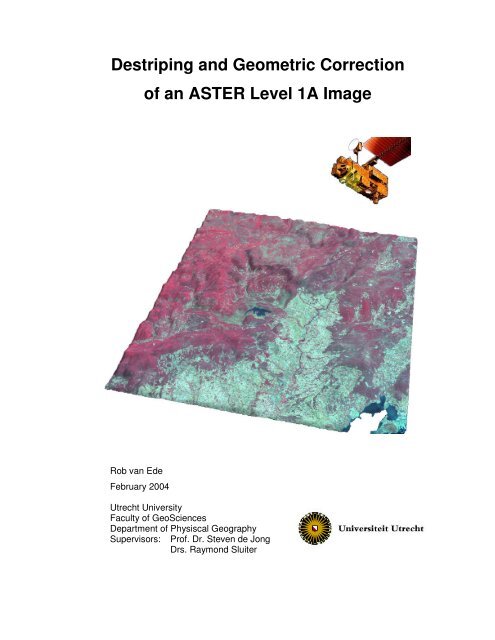
<strong>Destriping</strong> <strong><strong>an</strong>d</strong> <strong>Geometric</strong> <strong>Correction</strong><br />
Rob v<strong>an</strong> Ede<br />
February 2004<br />
<strong>of</strong> <strong>an</strong> <strong>ASTER</strong> <strong>Level</strong> 1A Image<br />
Utrecht University<br />
Faculty <strong>of</strong> GeoSciences<br />
Department <strong>of</strong> Physiscal Geography<br />
Supervisors: Pr<strong>of</strong>. Dr. Steven de Jong<br />
Drs. Raymond Sluiter
Contents<br />
List <strong>of</strong> tables 2<br />
List <strong>of</strong> figures 2<br />
1 Introduction 3<br />
2 Introduction to thermal remote sensing 4<br />
2.1 Blackbody radiation 4<br />
2.2 Real-world radiation 5<br />
3 The <strong>ASTER</strong> instrument 7<br />
3.1 VNIR telescope 7<br />
3.2 SWIR telescope 8<br />
3.3 TIR telescope 8<br />
3.4 Data Distribution: <strong>ASTER</strong> <strong>Level</strong>s 10<br />
4 Processing <strong>of</strong> the image 11<br />
4.1 Used <strong>ASTER</strong> image 11<br />
4.2 Processing s<strong>of</strong>tware 12<br />
4.3.1 Importing image data from <strong>ASTER</strong> HDF file 12<br />
4.3.2 <strong>Destriping</strong> 13<br />
4.3.3 DEM generation <strong><strong>an</strong>d</strong> orthorectification 13<br />
5 Accuracy assessment 17<br />
5.1 Source Data: EOS/HDF file 17<br />
5.2 <strong>Destriping</strong> 18<br />
5.3 DEM extraction 18<br />
5.4 Orthorectification 20<br />
6 Usability <strong>of</strong> <strong>ASTER</strong> imagery compared to DAIS 9715 imagery<br />
for thermal mapping 21<br />
6.1 Technical comparison <strong>ASTER</strong> versus DAIS 9615 21<br />
6.2 Data Quality 23<br />
6.3 Comparison <strong>of</strong> thermal products <strong>ASTER</strong> <strong><strong>an</strong>d</strong> DAIS 9615 24<br />
7 Conclusions 28<br />
8 References 29<br />
Appendix: <strong>ASTER</strong> correction HOWTO 30<br />
1
List <strong>of</strong> tables:<br />
Table 3.1: Spectral r<strong>an</strong>ge, resolution <strong><strong>an</strong>d</strong> bit depth (<strong>ASTER</strong> user guide)7<br />
Table 3.2: Gain settings for <strong>ASTER</strong> (<strong>ASTER</strong> user guide) 9<br />
Table 6.1: Technical properties <strong>of</strong> <strong>ASTER</strong> <strong><strong>an</strong>d</strong> DAIS 9715 sensors 22<br />
Table 6.2: Summary statistics for <strong>ASTER</strong> <strong><strong>an</strong>d</strong> DAIS9715 temperature<br />
List <strong>of</strong> figures:<br />
images 26<br />
Figure 2.1: Radi<strong>an</strong>ce <strong>of</strong> blackbody, graybody <strong><strong>an</strong>d</strong> selective radiator 5<br />
Figure 2.2: Location <strong>an</strong> b<strong><strong>an</strong>d</strong>width <strong>of</strong> <strong>ASTER</strong> b<strong><strong>an</strong>d</strong>s vs L<strong><strong>an</strong>d</strong>sat 7 9<br />
Figure 4.1: Overall workflow for geometric <strong><strong>an</strong>d</strong> radiometric correction 11<br />
Figure 4.2: SWIR b<strong><strong>an</strong>d</strong> 6,5,4 without <strong><strong>an</strong>d</strong> with parallax correction 14<br />
Figure 4.3: DEM generation from <strong>ASTER</strong> b<strong><strong>an</strong>d</strong> 3N <strong><strong>an</strong>d</strong> 3B stereo pair 15<br />
Figure 4.4: Workflow orthorectification <strong>of</strong> VNIR <strong><strong>an</strong>d</strong> SWIR b<strong><strong>an</strong>d</strong>s 16<br />
Figure 4.5: Workflow orthorectification TIR b<strong><strong>an</strong>d</strong>s 16<br />
Figure 5.1: Lateral shift <strong>ASTER</strong> image 17<br />
Figure 5.2: Generated DEM vs IGN reference DEM <strong><strong>an</strong>d</strong> location pr<strong>of</strong>ile 18<br />
Figure 6.1: Distortions resulting from non-ideal conditions in airborne<br />
remote sensing 24<br />
Figure 6.2: Temperature image from <strong>ASTER</strong> sensor 25<br />
Figure 6.3: Temperature image from DAIS sensor 25<br />
Figure 6.4: Differences DAIS – <strong>ASTER</strong> image 26<br />
2
1 Introduction<br />
The Adv<strong>an</strong>ced Spaceborne Thermal Emission <strong><strong>an</strong>d</strong> Reflection Radiometer<br />
(<strong>ASTER</strong>) is a multispectral sc<strong>an</strong>ner, developed by NASA, Jap<strong>an</strong>’s ministry <strong>of</strong><br />
Economy, Trade <strong><strong>an</strong>d</strong> Industry (METI) <strong><strong>an</strong>d</strong> the Earth Remote Sensing Data<br />
Analysis Center (ERSDAC). The <strong>ASTER</strong> sc<strong>an</strong>ner features sensors for<br />
measuring reflect<strong>an</strong>ce <strong><strong>an</strong>d</strong> radi<strong>an</strong>ce in parts <strong>of</strong> the visible, shortwave infrared<br />
<strong><strong>an</strong>d</strong> thermal infrared spectrum.<br />
Several processing steps are necessary before the data from the sensor are<br />
usable for research. What processing steps have to be performed depends on<br />
the actual usage <strong>of</strong> the data. In this paper, the radiometric <strong><strong>an</strong>d</strong> geometric<br />
correction <strong>of</strong> <strong>an</strong> <strong>ASTER</strong> <strong>Level</strong> 1A image <strong>of</strong> the Peyne catchment in Southern<br />
Fr<strong>an</strong>ce will be discussed <strong><strong>an</strong>d</strong> a step by step howto is included in the appendix.<br />
The paper is written to <strong>an</strong>swer the following question:<br />
What corrections have to be performed on <strong>an</strong> <strong>ASTER</strong> level 1A image in order<br />
to make the image usable for further research?<br />
In the last section, the properties <strong>of</strong> the <strong>ASTER</strong> sensor will be compared to<br />
the DAIS 9715 sensor that was used for thermal mapping <strong>of</strong> the Peyne<br />
catchment in 1998. Furthermore, a comparison <strong>of</strong> absolute temperature<br />
images on a sunny day in June from both sensors will be made.<br />
3
2 Introduction to thermal remote sensing<br />
In thermal remote sensing, radiation <strong>of</strong> objects is used to gather information<br />
on thermal properties <strong>of</strong> the objects under investigation. Thermal information<br />
<strong>of</strong> the surface provides information on moisture conditions <strong><strong>an</strong>d</strong><br />
evapo(tr<strong>an</strong>s)piration. In remote sensing, the radi<strong>an</strong>t temperature <strong>of</strong> <strong>an</strong> object<br />
c<strong>an</strong> be measured. Radi<strong>an</strong>t temperature differs from the kinetic temperature<br />
that is measured with a thermometer in direct contact with the object under<br />
investigation. The wavelengths used in thermal remote sensing are typically<br />
between 3 <strong><strong>an</strong>d</strong> 14 µm. The part between 8 <strong><strong>an</strong>d</strong> 14 µm is the most usable for<br />
thermal mapping. There are several reasons for this (Lilles<strong><strong>an</strong>d</strong> <strong><strong>an</strong>d</strong> Kiefer,<br />
2000):<br />
- There is <strong>an</strong> atmospheric window between 8 <strong><strong>an</strong>d</strong> 14 µm, so the<br />
atmosphere is reasonably tr<strong>an</strong>sparent to radiation in this r<strong>an</strong>ge.<br />
- Peak energy emissions from objects at the earth surface occur within<br />
this r<strong>an</strong>ge.<br />
- The radi<strong>an</strong>ce in the atmospheric window from 3 to 5 µm consists <strong>of</strong><br />
both reflected sunlight <strong><strong>an</strong>d</strong> emitted radi<strong>an</strong>ce from the earth surface.<br />
Both are difficult to separate.<br />
2.1 Blackbody radiation<br />
Every object with a surface temperature above 0 K radiates energy. This<br />
energy is radiated in a spectral distribution, typical for a material. If the object<br />
is a blackbody, the relation between the exit<strong>an</strong>ce peak <strong><strong>an</strong>d</strong> the surface<br />
temperature is described by Wien’s displacement law (Lilles<strong><strong>an</strong>d</strong> <strong><strong>an</strong>d</strong> Kiefer,<br />
2000):<br />
A<br />
m<br />
T<br />
= λ<br />
4
Where<br />
λ m = wavelength <strong>of</strong> maximum spectral radi<strong>an</strong>t exit<strong>an</strong>ce (µm)<br />
A = 2898 µm K<br />
T = Temperature (K)<br />
The Stef<strong>an</strong>-Bolzm<strong>an</strong>n law describes the total exit<strong>an</strong>ce from the surface <strong>of</strong> a<br />
blackbody in all wavelengths for a given temperature. The equation is as<br />
follows (Lilles<strong><strong>an</strong>d</strong> <strong><strong>an</strong>d</strong> Kiefer, 2000):<br />
∞<br />
∫<br />
0<br />
M = M ( λ ) dλ<br />
= σT<br />
Where<br />
4<br />
M = total radi<strong>an</strong>t exit<strong>an</strong>ce (W m -2 )<br />
0 = spectral radi<strong>an</strong>t exit<strong>an</strong>ce (W m -2 µm -1 )<br />
= Stef<strong>an</strong>-Bolzm<strong>an</strong>n const<strong>an</strong>t = 5.6697 X 10 -8 W m -2 K -4<br />
T = temperature <strong>of</strong> blackbody (K)<br />
As c<strong>an</strong> be seen from the Stef<strong>an</strong>-Bolzm<strong>an</strong>n law, the total radi<strong>an</strong>t exit<strong>an</strong>ce is<br />
directly related to the temperature <strong>of</strong> the blackbody. It is therefore possible to<br />
derive the temperature from measurements on radi<strong>an</strong>t exit<strong>an</strong>ce.<br />
2.2 Real-world radiation<br />
The total radi<strong>an</strong>t exit<strong>an</strong>ce <strong>of</strong> real objects is<br />
always lower th<strong>an</strong> the total radi<strong>an</strong>t exit<strong>an</strong>ce <strong>of</strong><br />
a blackbody, because real objects do not<br />
radiate energy in all wavelengths like a<br />
blackbody. For some objects the radi<strong>an</strong>t<br />
exit<strong>an</strong>ce curve has the same shape as the<br />
radi<strong>an</strong>t exit<strong>an</strong>ce curve <strong>of</strong> a blackbody, only<br />
lower. These objects radiate as a so called<br />
“graybody”. Other objects have a radi<strong>an</strong>t<br />
5<br />
Figure 2.1: Radi<strong>an</strong>ce <strong>of</strong> blackbody,<br />
graybody <strong><strong>an</strong>d</strong> selective radiator (Lilles<strong><strong>an</strong>d</strong><br />
<strong><strong>an</strong>d</strong> Kiefer, 1999)
exit<strong>an</strong>ce curve very different from that <strong>of</strong> a blackbody. These objects radiate<br />
as a “selective radiator”. Figure 1 shows the spectral radi<strong>an</strong>ce from these tree<br />
types <strong>of</strong> objects.<br />
If we w<strong>an</strong>t to distillate kinetic temperatures from the measured total radi<strong>an</strong>t<br />
exit<strong>an</strong>ce, then <strong>an</strong> extra variable has to be added to the Stef<strong>an</strong>-Bolzm<strong>an</strong>n<br />
equation to correct for the difference in radi<strong>an</strong>t exit<strong>an</strong>ce between a real object<br />
<strong><strong>an</strong>d</strong> a blackbody. When all objects are interpreted as a blackbody, then the<br />
measured temperatures will be lower <strong><strong>an</strong>d</strong> in some cases much lower th<strong>an</strong> the<br />
kinetic temperature <strong>of</strong> those objects.<br />
The variable that is added to the equation is the emissivity (ε). Emissivity<br />
describes the difference in energy radiation <strong>of</strong> <strong>an</strong> object compared to a<br />
blackbody (Lilles<strong><strong>an</strong>d</strong> <strong><strong>an</strong>d</strong> Kiefer, 2000):<br />
radi<strong>an</strong>t exit<strong>an</strong>ce <strong>of</strong> <strong>an</strong> object at a given temperature<br />
ε ( λ)<br />
=<br />
radi<strong>an</strong>t exit<strong>an</strong>ce <strong>of</strong> a blackbody at the same temperature<br />
For a graybody, the emissivity is the same for all wavelengths, but always<br />
lower th<strong>an</strong> 1. For a selective radiator, the emissivity ch<strong>an</strong>ges with wavelength.<br />
When broadb<strong><strong>an</strong>d</strong> sensors are used, the emissivity in the whole r<strong>an</strong>ge <strong>of</strong> the<br />
sensor is considered const<strong>an</strong>t like a graybody. For sensors equipped with<br />
multiple b<strong><strong>an</strong>d</strong>s in the thermal part <strong>of</strong> the spectrum, like the <strong>ASTER</strong> for<br />
example, multiple emissivity values c<strong>an</strong> be used on the different b<strong><strong>an</strong>d</strong>s to<br />
improve the result. With the split-window technique for example, atmospheric<br />
effects c<strong>an</strong> be derived from different emissivities in the thermal spectrum<br />
(César <strong><strong>an</strong>d</strong> Caselles, 1997). These differences in emissivity in adjacent b<strong><strong>an</strong>d</strong>s<br />
are closely correlated to the water vapor content <strong>of</strong> the atmosphere <strong><strong>an</strong>d</strong> air<br />
temperature pr<strong>of</strong>iles. Where vegetation behaves mostly like a graybody, soils<br />
show peaks <strong><strong>an</strong>d</strong> dips throughout the spectrum (Rubio et al, 1997).<br />
6
3 The <strong>ASTER</strong> instrument<br />
The Adv<strong>an</strong>ced Spaceborne Thermal Emission <strong><strong>an</strong>d</strong> Reflection Radiometer is a<br />
high resolution multispectral imaging device on board <strong>of</strong> NASA’s TERRA<br />
platform. TERRA was launched in December 1999 to a sun-synchronous,<br />
near polar orbit at 705 km altitude <strong><strong>an</strong>d</strong> crosses the equator at 10.30 local solar<br />
time. The orbit is the same every 16 days. Other devices on board the TERRA<br />
platform are MODIS, MISR, CERES <strong><strong>an</strong>d</strong> MOPITT.<br />
The <strong>ASTER</strong> records data in 14 spectral b<strong><strong>an</strong>d</strong>s: 3 b<strong><strong>an</strong>d</strong>s in Visible Near-<br />
InfraRed (VNIR) with 15 meter spatial resolution, 6 b<strong><strong>an</strong>d</strong>s in Short Wave<br />
InfraRed (SWIR) with 30 meter spatial resolution <strong><strong>an</strong>d</strong> 5 b<strong><strong>an</strong>d</strong>s in Thermal<br />
InfraRed (TIR) with 90 meter spatial resolution. Detailed properties <strong>of</strong> these<br />
b<strong><strong>an</strong>d</strong>s are given in table 1 <strong><strong>an</strong>d</strong> figure 2:<br />
Table 3.1: Spectral r<strong>an</strong>ge, resolution <strong><strong>an</strong>d</strong> bit depth (Abrams et al., 2002, http://asterweb.jpl.nasa.gov)<br />
3.1 VNIR telescope<br />
The VNIR system consists <strong>of</strong> three line arrays <strong>of</strong> 5000 CCD sensors each <strong>of</strong><br />
which 4100 are used. Wavelength discrimination is done with a dichroic prism<br />
<strong><strong>an</strong>d</strong> interference filters. No rotating mirrors are used in the VNIR system. Each<br />
b<strong><strong>an</strong>d</strong> has three gain settings for adaptation to different radi<strong>an</strong>ce levels without<br />
losing bit resolution (Table 2). Very different radi<strong>an</strong>ce levels are encountered<br />
at different location <strong><strong>an</strong>d</strong> time. In Arctic regions for example, reflection is very<br />
7
high as a result <strong>of</strong> the high albedo <strong>of</strong> snow. For such a region, a low gain<br />
setting may be used to prevent the sensor from overloading. In low light<br />
conditions, a higher gain setting may be used to increase the sensitivity <strong>of</strong> the<br />
sensor <strong><strong>an</strong>d</strong> make small reflections visible. For every gain setting, there is a<br />
conversion coefficient in the telescope specific metadata to convert the digital<br />
numbers from the sensor to radi<strong>an</strong>ce at the sensor using the following<br />
equation (Abrams et al., 2002):<br />
Radi<strong>an</strong>ce = (DN value –1) * conversion coefficient<br />
For DEM extraction there is <strong>an</strong>other array <strong>of</strong> sensors identical to b<strong><strong>an</strong>d</strong> 3, but<br />
pointed backwards. Radiometric accuracy for the VNIR system is ±4 % or<br />
better.<br />
3.2 SWIR telescope<br />
The SWIR system uses a Platinum Silicide-Silicon Schottky barrier linear<br />
array <strong>of</strong> 2048 detectors for each <strong>of</strong> the six b<strong><strong>an</strong>d</strong>s. For wavelength separation,<br />
optical b<strong><strong>an</strong>d</strong> pass filters are used. Radiometric accuracy for the SWIR system<br />
is +4 % or better. Four gain settings are available (Table 2). Conversion to<br />
radi<strong>an</strong>ce is the same as for the VNIR b<strong><strong>an</strong>d</strong>s.<br />
3.3 TIR telescope<br />
The TIR system uses a Newtoni<strong>an</strong> catadioptric sc<strong>an</strong>ning system with 10<br />
Mercury-Cadmium-Telluride detectors per b<strong><strong>an</strong>d</strong> in a staggered array. Like the<br />
SWIR system, optical b<strong><strong>an</strong>d</strong> pass filters are used for wavelength separation. A<br />
moving mirror is used for pointing <strong><strong>an</strong>d</strong> sc<strong>an</strong>ning. For calibration, there is a<br />
blackbody <strong>of</strong> which the temperature c<strong>an</strong> be ch<strong>an</strong>ged. As c<strong>an</strong> be seen in Table<br />
2, only one gain setting is available, but the TIR sensor has <strong>an</strong> increased bit<br />
depth.<br />
8
Table 3.2: Gain settings for <strong>ASTER</strong> sensors (Abrams et al., 2002, http://asterweb.jpl.nasa.gov)<br />
Figure 2.2: Location <strong><strong>an</strong>d</strong> b<strong><strong>an</strong>d</strong>width <strong>of</strong> <strong>ASTER</strong> b<strong><strong>an</strong>d</strong>s compared to L<strong><strong>an</strong>d</strong>sat 7 b<strong><strong>an</strong>d</strong>s (Abrams et al.,<br />
2002, http://asterweb.jpl.nasa.gov)<br />
9
3.3 Data distribution: <strong>ASTER</strong> <strong>Level</strong>s<br />
<strong>ASTER</strong> data are available in several processing levels. <strong>Level</strong> 1 data contain<br />
data for all b<strong><strong>an</strong>d</strong>s <strong>of</strong> the <strong>ASTER</strong> instrument. Higher level data are products are<br />
derived from level 1 data. There are two level one data products: <strong>Level</strong> 1A<br />
<strong><strong>an</strong>d</strong> <strong>Level</strong> 1B.<br />
<strong>Level</strong> 1A data contain unprocessed digital counts for each b<strong><strong>an</strong>d</strong> at full<br />
resolution. The coefficients for conversion to at-sensor radi<strong>an</strong>ce <strong><strong>an</strong>d</strong><br />
geometric correction are supplied in the metadata, but no tr<strong>an</strong>sformations are<br />
applied. Because no tr<strong>an</strong>sformations have been applied, <strong>Level</strong> 1A data are a<br />
good source for DTM extraction, which will be discussed in this paper. All data<br />
collected by <strong>ASTER</strong> is processed to <strong>Level</strong> 1A data.<br />
In <strong>Level</strong> 1B data, the raw digital counts <strong>of</strong> <strong>Level</strong> 1A data are converted to<br />
radi<strong>an</strong>ce values, <strong><strong>an</strong>d</strong> a tr<strong>an</strong>sformation has been applied to register the image<br />
to a coordinate system. Because the data were resampled, level 1B data are<br />
less suitable for DTM extraction. <strong>Level</strong> 1B c<strong>an</strong> however be used for spectral<br />
<strong>an</strong>alysis without <strong>an</strong>y preprocessing. Only cloudless scenes are processed to<br />
<strong>Level</strong> 1B.<br />
10
4 Processing <strong>of</strong> the image<br />
Before satellite imagery c<strong>an</strong> be used as a data source for research <strong>of</strong> the<br />
earth surface <strong><strong>an</strong>d</strong> / or atmosphere, the raw sensor data must be processed to<br />
derive useful information from the digital numbers produced by the sensors.<br />
The most basic, but necessary processing involves geometric <strong><strong>an</strong>d</strong> radiometric<br />
correction. When these corrections are applied, the image is registered to a<br />
coordinate system, so the location <strong>of</strong> every pixel at the earth surface is known<br />
<strong><strong>an</strong>d</strong> the digital numbers are converted to radi<strong>an</strong>ce. This radi<strong>an</strong>ce values c<strong>an</strong><br />
th<strong>an</strong> be converted into surface reflect<strong>an</strong>ce or brightness temperature.<br />
The procedure for geometric correction <strong><strong>an</strong>d</strong> radiometric correction to at-<br />
sensor radi<strong>an</strong>ce is described in this paper. <strong>Correction</strong> <strong>of</strong> atmospheric effects<br />
was not performed. Because there was some striping present in some <strong>of</strong> the<br />
b<strong><strong>an</strong>d</strong>s, those b<strong><strong>an</strong>d</strong>s were destriped in order to remove the striping artifacts<br />
from the image data. The flowchart below (fig. 4.1) shows the overall workflow<br />
for the correction process. The different parts <strong>of</strong> this workflow will be<br />
discussed in detail in the following sections.<br />
<strong>ASTER</strong> HDF<br />
file<br />
HDF Import<br />
Image data<br />
<strong>Destriping</strong><br />
11<br />
Orthorectification<br />
METAdata DEM extraction<br />
DEM<br />
Figure 4.1: Overall workflow for geometric <strong><strong>an</strong>d</strong> radiometric correction <strong>ASTER</strong> <strong>Level</strong> 1A images<br />
4.1 Used <strong>ASTER</strong> image<br />
Orthorectified<br />
B<strong><strong>an</strong>d</strong>s<br />
The used image is <strong>an</strong> <strong>ASTER</strong> <strong>Level</strong> 1A image <strong>of</strong> the Peyne area in Southern<br />
Fr<strong>an</strong>ce <strong><strong>an</strong>d</strong> was acquired on June 13 th 2002. All <strong>ASTER</strong> sensors (VNIR,<br />
SWIR <strong><strong>an</strong>d</strong> TIR) were active <strong><strong>an</strong>d</strong> the image is free from clouds. Some b<strong><strong>an</strong>d</strong>s<br />
suffer from striping. <strong>ASTER</strong> <strong>Level</strong> 1A image comprise a data format with no<br />
geometric <strong><strong>an</strong>d</strong> radiometric correction applied to the image. All correction<br />
coefficients are supplied in the header <strong>of</strong> the HDF file. These coefficients were<br />
extracted from the metadata <strong><strong>an</strong>d</strong> used for radiometric correction.
4.2 Processing s<strong>of</strong>tware<br />
All processing was carried out in two image processing programs: Erdas<br />
Imagine 8.6 (http://www.gis.leica-geosystems.com) <strong><strong>an</strong>d</strong> Research Systems<br />
ENVI 3.5 (http://www.rsinc.com/envi). Erdas Imagine has al the functionality<br />
that is needed except for rotating the image, which was done in ENVI. The<br />
destripe algorithms in both programs give different results, so for the given<br />
data, the best algorithm c<strong>an</strong> be chosen.<br />
4.3.1 Importing image data from <strong>ASTER</strong> HDF file<br />
Erdas Imagine version 8.6 now contains <strong>an</strong> <strong>ASTER</strong> HDF importer that c<strong>an</strong> do<br />
both geometric <strong><strong>an</strong>d</strong> radiometric correction <strong>of</strong> the data. Because there was<br />
some striping in the image, only the automatic radiometric correction from this<br />
import utility was used. For the automatic radiometric correction, the digital<br />
numbers are multiplied by a coefficient that depends from the gain setting <strong>of</strong><br />
the sensor (Table 2). These coefficients are supplied in the metadata.<br />
Striping is usually caused by some sensors that are out <strong>of</strong> alignment,<br />
defective or not calibrated correctly. This results in rows or columns in the<br />
image that deviate from neighboring rows or columns <strong><strong>an</strong>d</strong> c<strong>an</strong> hamper<br />
subsequent processing. The destriping algorithms used in Imagine <strong><strong>an</strong>d</strong> ENVI<br />
were originally designed to destripe L<strong><strong>an</strong>d</strong>sat TM images that contain<br />
horizontal striping because one <strong>of</strong> L<strong><strong>an</strong>d</strong>sat’s sensors was out <strong>of</strong> alignment.<br />
When the automatic geometric correction <strong>of</strong> the <strong>ASTER</strong> HDF importer is used,<br />
the image is resampled <strong><strong>an</strong>d</strong> no longer contains perfect vertical (VNIR, SWIR)<br />
or horizontal (TIR) striping (it was vertical because <strong>ASTER</strong> uses <strong>an</strong> array <strong>of</strong><br />
sensors instead <strong>of</strong> a pointing mirror <strong><strong>an</strong>d</strong> a small number <strong>of</strong> sensors for the<br />
VNIR <strong><strong>an</strong>d</strong> SWIR b<strong><strong>an</strong>d</strong>s, like L<strong><strong>an</strong>d</strong>sat). If the geometric correction <strong>of</strong> the<br />
importer is used <strong><strong>an</strong>d</strong> the image is resampled, the destriped algorithm does not<br />
work. <strong>Geometric</strong> correction thus has to be done by h<strong><strong>an</strong>d</strong>, after the striping has<br />
been removed.<br />
12
4.3.2 <strong>Destriping</strong><br />
The destriping algorithm used in ENVI calculates the me<strong>an</strong> for each line <strong><strong>an</strong>d</strong><br />
then normalizes the line to this me<strong>an</strong>. The periodicity <strong>of</strong> the striping is filled in<br />
as the number <strong>of</strong> sensors. For the destriping algorithm to work, the striping in<br />
the image should thus have a horizontal orientation. Because both the VNIR<br />
<strong><strong>an</strong>d</strong> SWIR sensors use <strong>an</strong> array <strong>of</strong> sensors perpendicular to the flight<br />
direction, possible striping from miscalibrated sensors will occur in a vertical<br />
orientation, <strong><strong>an</strong>d</strong> not horizontal as in L<strong><strong>an</strong>d</strong>sat images. As a result <strong>of</strong> this, the<br />
image has to be rotated prior to applying a destriping algorithm. It is best to<br />
rotate the image by 270 degrees, because the images will have the right<br />
orientation compared to each other for use in Orthobase that way. When<br />
rotated by only 90 degrees, destriping c<strong>an</strong> be performed, but will not be<br />
displayed properly on Orthobase. Because the TIR sensor uses a moving<br />
mirror for sc<strong>an</strong>ning, the striping is already oriented horizontally <strong><strong>an</strong>d</strong> thus no<br />
rotation has to be performed.<br />
After the rotation, actual destriping c<strong>an</strong> be performed. While a different sensor<br />
is used for every column <strong>of</strong> the image (4100 sensors for VNIR, 2048 for<br />
SWIR, 700 for TIR), the number <strong>of</strong> sensors for destriping has to be set to 2. If<br />
the number <strong>of</strong> sensors is set to the actual number <strong>of</strong> sensors for each b<strong><strong>an</strong>d</strong>,<br />
the output values differ considerably from the input values <strong><strong>an</strong>d</strong> data quality is<br />
compromised.<br />
4.3.3 DEM generation <strong><strong>an</strong>d</strong> orthorectification<br />
After the images have been destriped properly, orthorectification c<strong>an</strong> be<br />
performed to georeference the images <strong><strong>an</strong>d</strong> correct for errors in image<br />
coordinates due to relief displacement, earth curvature <strong><strong>an</strong>d</strong> inter- <strong><strong>an</strong>d</strong> intra-<br />
telescope parallax errors. Especially the SWIR b<strong><strong>an</strong>d</strong>s suffer from parallax<br />
errors because the sensor arrays for the different b<strong><strong>an</strong>d</strong>s are not perfectly<br />
aligned. This results in b<strong><strong>an</strong>d</strong>s that are shifted in space relative to each other.<br />
13
In the used image, this shift was in the order <strong>of</strong> 10 pixels per b<strong><strong>an</strong>d</strong> (300 meter)<br />
<strong><strong>an</strong>d</strong> thus has a very large impact on image quality if it is not corrected. When<br />
the st<strong><strong>an</strong>d</strong>ard geometric correction from the import-utility is used, the parallax<br />
correction is automatically applied, but then the destriping algorithms are not<br />
usable <strong>an</strong>ymore (except for a Fourier Tr<strong>an</strong>sform) as discussed in chapter<br />
4.3.1. Figure 4.2 below shows a part <strong>of</strong> the image before correction <strong><strong>an</strong>d</strong> the<br />
edge <strong>of</strong> the image after correction so that the amount <strong>of</strong> shift needed for<br />
correction is visible.<br />
Figure 4.2: SWIR b<strong><strong>an</strong>d</strong> 6,5,4 without <strong><strong>an</strong>d</strong> with parallax correction<br />
A method for correcting for geometric errors in the image is orthorectification<br />
with a DEM (Digital Elevation Model) as input. When orthorectification is<br />
performed, all errors mentioned above are corrected in the same process. The<br />
backward looking <strong>ASTER</strong> b<strong><strong>an</strong>d</strong> c<strong>an</strong> be used for DEM generation, so there is<br />
no external DEM needed for the orthorectification. Erdas Orthobase pro<br />
contains al the tools for DEM extraction from stereo image sources <strong><strong>an</strong>d</strong><br />
orthorectification. Because the DEM is needed as <strong>an</strong> input for<br />
orthorectification, the first step that has to be performed is DEM extraction.<br />
The workflow is outlined in the flowchart below (Figure 4.3):<br />
14
B<strong><strong>an</strong>d</strong> 3 Nadir<br />
B<strong><strong>an</strong>d</strong> 3 Back<br />
Rotation<br />
Rotation<br />
<strong>Destriping</strong><br />
<strong>Destriping</strong><br />
Topographic<br />
Map<br />
Collect<br />
GCP’s<br />
Auto Tie Point<br />
generation<br />
Figure 4.3: DEM generation from <strong>ASTER</strong> b<strong><strong>an</strong>d</strong> 3N <strong><strong>an</strong>d</strong> 3B stereo pair<br />
15<br />
Tri<strong>an</strong>gulation DEM extraction<br />
DEM<br />
Orthorectification<br />
Both b<strong><strong>an</strong>d</strong>s are rotated by 270 degrees so that they overlap properly.<br />
B<strong><strong>an</strong>d</strong> 3 Nadir<br />
orthorectified<br />
B<strong><strong>an</strong>d</strong> 3 Back<br />
orthorectified<br />
<strong>Destriping</strong> is performed as described in paragraph 4.3.1 to remove possible<br />
striping from both images.<br />
The value for side incidence is extracted from metadata <strong><strong>an</strong>d</strong> used for setting<br />
up Orthobase.<br />
Ground Control Points are located from locations with known x, y <strong><strong>an</strong>d</strong> z<br />
coordinates in both images. For high quality DEM extraction from <strong>an</strong> <strong>ASTER</strong><br />
scene, 54 to 74 GCP’s are recommended (Geosystems, 2002). All GCP’s<br />
were measured from topographic maps at a scale <strong>of</strong> 1:25000.<br />
After sufficient GCP’s have been located, 200 automatic tie points<br />
(Geosystems, 2002) should be generated <strong><strong>an</strong>d</strong> tri<strong>an</strong>gulation c<strong>an</strong> be performed.<br />
The last step is the DEM generation itself, after which the generated DEM c<strong>an</strong><br />
be used for orthorectifieing the two images. The cubic convolution resampling<br />
method was used, because this method produces a sharper image th<strong>an</strong> other<br />
interpolation methods. The downside <strong>of</strong> the cubic convolution method is that it<br />
applies a smoothing to the pixel values (Lilles<strong><strong>an</strong>d</strong>, Kiefer, 2000).<br />
The orthorectified b<strong><strong>an</strong>d</strong> 3N <strong><strong>an</strong>d</strong> the DEM c<strong>an</strong> now be used as a source for<br />
orthorectification <strong>of</strong> the other <strong>ASTER</strong> b<strong><strong>an</strong>d</strong>s. The workflow for the entire<br />
process (destriping <strong><strong>an</strong>d</strong> orthorectification) is outlined in the flowcharts below.<br />
For the thermal b<strong><strong>an</strong>d</strong>s, no rotation is necessary because <strong>an</strong>y striping present<br />
is already horizontal.
VNIR / SWIR<br />
input B<strong><strong>an</strong>d</strong><br />
Conversion to<br />
Radi<strong>an</strong>ce<br />
Rotation <strong>Destriping</strong><br />
Orthorectified B<strong><strong>an</strong>d</strong><br />
3 Nadir<br />
Collect<br />
GCP’s<br />
Figure 4.4: Workflow orthorectification <strong>of</strong> VNIR <strong><strong>an</strong>d</strong> SWIR b<strong><strong>an</strong>d</strong>s<br />
VNIR / SWIR<br />
input B<strong><strong>an</strong>d</strong><br />
Conversion to<br />
Radi<strong>an</strong>ce<br />
<strong>Destriping</strong><br />
Orthorectified B<strong><strong>an</strong>d</strong><br />
3 Nadir<br />
Collect<br />
GCP’s<br />
Figure 4.5: Workflow orthorectification <strong>of</strong> TIR b<strong><strong>an</strong>d</strong>s<br />
Auto Tie Point<br />
generation<br />
16<br />
Auto Tie Point<br />
generation<br />
Tri<strong>an</strong>gulation Orthorectification<br />
Tri<strong>an</strong>gulation Orthorectification<br />
B<strong><strong>an</strong>d</strong><br />
orthorectified<br />
B<strong><strong>an</strong>d</strong><br />
orthorectified
5 Accuracy assessment<br />
The accuracy <strong>of</strong> the final product depends on the quality <strong>of</strong> the input data<br />
(rubbish in, rubbish out) <strong><strong>an</strong>d</strong> on the accuracy <strong>of</strong> all processing that is<br />
performed on the data. Therefore, every step in the workflow will be discussed<br />
in order to get some insight in the final accuracy <strong>of</strong> the end product.<br />
5.1 Source data: HDF/EOS file:<br />
Only images acquired by the <strong>ASTER</strong> that have low cloud coverage are<br />
normally processed to <strong>Level</strong> 1 data. Data for all b<strong><strong>an</strong>d</strong>s is distributed in one<br />
HDF file <strong><strong>an</strong>d</strong> in the case <strong>of</strong> a level 1A image as discussed in this paper, the<br />
images are not georeferenced or processed to radi<strong>an</strong>ce. With the help <strong>of</strong> the<br />
metadata supplied in the HDF file, the image c<strong>an</strong> be georeferenced <strong><strong>an</strong>d</strong><br />
radiometric correction c<strong>an</strong> be performed to get top-<strong>of</strong>-atmosphere radi<strong>an</strong>ce.<br />
Atmospheric conditions c<strong>an</strong> have signific<strong>an</strong>t impact on passing radiation<br />
(absorption, scatter). This top-<strong>of</strong>-atmosphere radi<strong>an</strong>ce therefore c<strong>an</strong> be<br />
different from the actual surface radi<strong>an</strong>ce <strong><strong>an</strong>d</strong> this is why it may be necessary<br />
to correct for atmospheric effects.<br />
The coefficients for georeferencing that are supplied in the metadata have<br />
proven to be <strong>of</strong> limited use. For the global position <strong>of</strong> the image, automatic<br />
georeferencing is fine, but if the data have to be used in conjunction with other<br />
data (like in most studies), the error <strong>of</strong> several pixels is too large (figure 5.1).<br />
Figure 5.1: Lateral shift <strong>ASTER</strong> image (see crosshair)<br />
17
Parallax errors, especially in the SWIR telescope, are <strong>an</strong>other source <strong>of</strong> error<br />
that has to be corrected for (see 4.3.3), like parallax errors resulting from<br />
elevation differences.<br />
5.2 <strong>Destriping</strong>:<br />
Remotely sensed images <strong>of</strong>ten contain striping <strong><strong>an</strong>d</strong> <strong>ASTER</strong> images are no<br />
different. Especially the SWIR b<strong><strong>an</strong>d</strong>s contained striping, which was reduced<br />
with a destriping algorithm from either Imagine or ENVI. The destriping<br />
algorithm in ENVI seems to work less rigorous th<strong>an</strong> the algorithm in Imagine.<br />
Which algorithm should be used thus depends on the nature <strong>of</strong> the striping in<br />
the image. Only b<strong><strong>an</strong>d</strong>s with heavy <strong><strong>an</strong>d</strong> uneven striping, like SWIR b<strong><strong>an</strong>d</strong> 4 <strong><strong>an</strong>d</strong><br />
the TIR b<strong><strong>an</strong>d</strong>s were destriped in Imagine.<br />
An other method for destriping, Fourier <strong>an</strong>alysis, was not used because it is<br />
very labor intensive to setup <strong><strong>an</strong>d</strong> results in very long computation times.<br />
5.3 DEM extraction:<br />
In this paper, orthorectification on the basis <strong>of</strong> the extracted DEM was used to<br />
correct for all geometric errors. DEM extraction <strong><strong>an</strong>d</strong> orthorectification rely on<br />
the quality <strong>of</strong> the used Ground Control Points. The source for these GCPs<br />
were several 1:25.000 topographic maps. The actual quality <strong>of</strong> these maps is<br />
not known. During the measuring <strong>of</strong> GCPs, one <strong>of</strong> the used maps showed a<br />
shift <strong>of</strong> approximately 10 meters compared to the other maps <strong><strong>an</strong>d</strong> this may be<br />
one <strong>of</strong> the causes for the height exaggeration discussed below. The total RMS<br />
error for the GCPs during tri<strong>an</strong>gulation is 0.8664 pixels for X <strong><strong>an</strong>d</strong> 0.8391 pixels<br />
for Y. This equates to 13 meters for X <strong><strong>an</strong>d</strong> 12.6 meters for Y.<br />
The extracted DEM has 83 meter grid cells, which is half the grid cell size that<br />
was suggested by orthobase. By using relatively large grid cells, errors from<br />
the DEM extraction are smoothed out, reducing noise. The high altitude <strong>of</strong> the<br />
spacecraft (705 km) compared to the elevation differences in the image (1 km)<br />
18
makes the grid cell size <strong>of</strong> the DEM less import<strong>an</strong>t when it is used for<br />
orthorectification only: correction is only necessary for large terrain features<br />
that are perfectly visible in a DEM with a large grid cell size.<br />
The extracted DEM was compared to a reference DEM with 25 meter grid<br />
cells from IGN <strong>of</strong> a part <strong>of</strong> the area. In most <strong>of</strong> the area, the generated DEM<br />
overestimates the elevation by sometimes 50 meters (figure 5.2). Close to the<br />
sea, where elevations are low, the generated DEM shows elevations below<br />
sea level where the reference DEM shows positive elevations.<br />
From this comparison, it seems that the extracted DEM exaggerates the relief<br />
by some degree. While this may be a problem when exact heights are<br />
needed, this is much less <strong>of</strong> a problem when the DEM is used for<br />
orthorectification only, as in this paper. Overall, the extracted DEM <strong><strong>an</strong>d</strong> the<br />
reference DEM are very much alike.<br />
Figure 5.2: Generated DEM (red line) versus IGN reference DEM (green line) <strong><strong>an</strong>d</strong> location pr<strong>of</strong>ile<br />
5.4 Orthorectification:<br />
For orthorectification, again the GCPs are import<strong>an</strong>t. Because some terrain<br />
features have very different reflect<strong>an</strong>ce / radi<strong>an</strong>ce properties in different<br />
b<strong><strong>an</strong>d</strong>s, it is sometimes hard to identify the same feature in <strong>an</strong>other b<strong><strong>an</strong>d</strong>. As a<br />
result <strong>of</strong> this, the number <strong>of</strong> GCPs that c<strong>an</strong> be found decreases. For<br />
orthorectification, a minimum <strong>of</strong> seven GCPs per b<strong><strong>an</strong>d</strong> were used because<br />
sometimes no more reliable GCPs could be found. The courser resolution <strong>of</strong><br />
the SWIR <strong><strong>an</strong>d</strong> TIR b<strong><strong>an</strong>d</strong>s also lowers the accuracy for the GCPs <strong><strong>an</strong>d</strong> <strong>of</strong>ten the<br />
middle <strong>of</strong> a pixel is used to reference a feature. In the case <strong>of</strong> features smaller<br />
19
th<strong>an</strong> a pixel, this feature may be positioned <strong>an</strong>ywhere in that pixel <strong><strong>an</strong>d</strong> the<br />
exact location is not known. The measuring errors created by this show up<br />
during tri<strong>an</strong>gulation as a higher RMS error.<br />
After orthorectification, most <strong>of</strong> the parallax errors in the SWIR b<strong><strong>an</strong>d</strong>s was<br />
removed. Some very small (
6 Usability <strong>of</strong> <strong>ASTER</strong> imagery compared to DAIS 9715 imagery for<br />
thermal mapping<br />
From the field study carried out by Eva Koster <strong><strong>an</strong>d</strong> Arko Lucieer in 1998,<br />
extensive information is available on the thermal properties <strong>of</strong> the Peyne<br />
catchment. Also, the perform<strong>an</strong>ce <strong>of</strong> the experimental DAIS airborne sc<strong>an</strong>ner<br />
<strong><strong>an</strong>d</strong> the necessary processing steps for deriving the surface temperature from<br />
DAIS imagery is discussed. An <strong>ASTER</strong> image that covers the same area is<br />
now available. Having data from two sc<strong>an</strong>ners <strong>of</strong> the same area is <strong>an</strong><br />
opportunity to compare the perform<strong>an</strong>ce <strong>of</strong> both sc<strong>an</strong>ners. In the following<br />
sections, the comparison will be focused on the technical properties <strong>of</strong> both<br />
sc<strong>an</strong>ners.<br />
6.1 Technical comparison <strong>ASTER</strong> versus DAIS 9715<br />
While both sensors cover approximately the same wavelength r<strong>an</strong>ge, they do<br />
so in different ways. <strong>ASTER</strong> collects data in tree atmospheric windows: VNIR,<br />
SWIR <strong><strong>an</strong>d</strong> TIR. DAIS collects data in four atmospheric windows: VNIR, SWIR,<br />
MIR <strong><strong>an</strong>d</strong> TIR. <strong>ASTER</strong> uses only 14 relatively wideb<strong><strong>an</strong>d</strong> sensors, were DAIS<br />
uses 79 sensors. Some <strong>of</strong> the DAIS b<strong><strong>an</strong>d</strong>s are very narrow, while others<br />
cover a larger b<strong><strong>an</strong>d</strong>width.<br />
The spatial resolution is the same for all b<strong><strong>an</strong>d</strong>s <strong>of</strong> the DAIS sensor, which<br />
me<strong>an</strong>s that data for every covered wavelength are available at the same pixel<br />
size. In this way, it is relatively easy to link for example optical to thermal data.<br />
<strong>ASTER</strong> uses a different spatial resolution for the different wavelength r<strong>an</strong>ges.<br />
This me<strong>an</strong>s that data are collected at different resolutions <strong><strong>an</strong>d</strong> some additional<br />
processing is required to link these data.<br />
For the VNIR <strong><strong>an</strong>d</strong> SWIR b<strong><strong>an</strong>d</strong>s, <strong>ASTER</strong> utilizes no rotating mirrors, but a<br />
separate sensor for each pixel. This absence <strong>of</strong> rotating parts guar<strong>an</strong>ties a<br />
consistent quality throughout sensor life, not compromised by mech<strong>an</strong>ical<br />
wear or vibrations. The use <strong>of</strong> m<strong>an</strong>y sensors requires all sensors to be<br />
calibrated very accurately, or striping will occur in the way described above.<br />
The moving mirrors used in the DAIS sensor are susceptible to vibration, for<br />
21
example from the engine <strong>of</strong> the airpl<strong>an</strong>e in which it is installed (Strobl, 1996).<br />
This also results in striping.<br />
In table 6.1, the technical properties <strong>of</strong> both sensors are listed:<br />
<strong>ASTER</strong> DAIS 9715<br />
Number <strong>of</strong> b<strong><strong>an</strong>d</strong>s VNIR: 3 + back looking VNIR: 32<br />
SWIR: 6 SWIR1: 8<br />
22<br />
SWIR2: 32<br />
MIR: 1<br />
TIR: 5 TIR: 6<br />
Spatial resolution VNIR: 15 m depends on altitude,<br />
SWIR: 30 m identical for all ch<strong>an</strong>nels<br />
TIR: 90 m typically 7 m (at 3000 m<br />
altitude)<br />
Wavelength r<strong>an</strong>ge VNIR: 0.52 – 0.86 µm VNIR: 0.4 – 1.0 µm<br />
SWIR: 1.60 – 2.43 µm SWIR1: 1.5 – 1.8 µm<br />
SWIR2: 2.0 – 2.5 µm<br />
MIR: 3.0 – 5.0 µm<br />
TIR: 8.125 – 11.65 µm TIR: 8.7 – 12.3 µm<br />
B<strong><strong>an</strong>d</strong>width VNIR: 0.60 – 0.80 µm VNIR: 12 – 35 nm<br />
SWIR: 40 – 70 nm SWIR1: 36 – 56 nm<br />
SWIR2: 20 – 40 nm<br />
MIR: 2.0 µm<br />
TIR: 0.35 – 0.70 µm TIR: 0.6 – 1.0 µm<br />
Table 6.1: Technical properties <strong>of</strong> <strong>ASTER</strong> <strong><strong>an</strong>d</strong> DAIS 9715 sensors (collected from Abrams et al., 2002 <strong><strong>an</strong>d</strong><br />
Strobl, 1996)
6.2 Data quality<br />
The data acquired by both sensors do not only differ in qu<strong>an</strong>tity, but also in<br />
quality. In remotely sensed images, distortion may be <strong>of</strong> geometric or<br />
radiometric nature. Radiometric distortion c<strong>an</strong> be caused by instrument<br />
miscalibration or atmospheric effects (Lilles<strong><strong>an</strong>d</strong> <strong>an</strong> Kiefer, 2000). When <strong>an</strong><br />
instrument uses sensors that work reliably <strong><strong>an</strong>d</strong> as specified, lookup tables c<strong>an</strong><br />
be used to retrieve data with good radiometric quality.<br />
The radi<strong>an</strong>ce measured by the sensor is called the at-sensor radi<strong>an</strong>ce. The<br />
atmosphere between the sensor <strong><strong>an</strong>d</strong> the earth surface has influence on<br />
passing radiation, <strong><strong>an</strong>d</strong> thus on the final measurement. As the DAIS sensor<br />
was operated from <strong>an</strong> airpl<strong>an</strong>e at <strong>an</strong> altitude <strong>of</strong> 3000 meter <strong><strong>an</strong>d</strong> <strong>ASTER</strong> is<br />
onboard the TERRA platform at <strong>an</strong> altitude <strong>of</strong> 705.000 meter, there is much<br />
more atmosphere between <strong>ASTER</strong> <strong><strong>an</strong>d</strong> the earth surface th<strong>an</strong> there is<br />
between DAIS <strong><strong>an</strong>d</strong> the earth surface. A longer path trough the atmosphere<br />
me<strong>an</strong>s more potential influence <strong>of</strong> the atmosphere on the radiation that has to<br />
be corrected for. There are different methods for atmospheric correction. One<br />
simple method is the darkest pixel method, in which the value <strong>of</strong> a pixel that is<br />
assumed to be black (like deep, clear water) is subtracted from all pixels in<br />
that b<strong><strong>an</strong>d</strong>. Another method, that requires field measurements, is the empirical<br />
line method. In the empirical line method, field measured reflect<strong>an</strong>ce /<br />
exit<strong>an</strong>ce values are used to remove atmospheric influence in the image using<br />
linear regression. A third method for atmospheric correction is a computer<br />
based model such as MODTRAN or ACORN. These models require additional<br />
information on atmospheric conditions when the image was acquired <strong><strong>an</strong>d</strong><br />
thus, more uncertainties are introduced. The required additional data for<br />
ACORN are atmospheric visibility <strong><strong>an</strong>d</strong> fixed water vapor (Imspec, 2002).<br />
Because DAIS is <strong>an</strong> airborne sc<strong>an</strong>ner <strong><strong>an</strong>d</strong> <strong>ASTER</strong> is onboard a spacecraft,<br />
<strong>ASTER</strong> moves in a more steady <strong><strong>an</strong>d</strong> predictable way th<strong>an</strong> DAIS, which is<br />
much more prone to variations in the flight path. Figure 6.1 shows these<br />
variations, along with the resulting geometric errors in the recorded image. In<br />
spaceborne remote sensing, these problems do not exist.<br />
23
Vibrations from the airpl<strong>an</strong>e may have influence on data quality. Severe<br />
striping in some <strong>of</strong> the SWIR b<strong><strong>an</strong>d</strong>s in the DAIS image was caused by<br />
vibrations <strong>of</strong> the engines (Strobl, 1996).<br />
Figure 6.1: Distortions resulting from non-ideal conditions in airborne remote sensing (Lilles<strong><strong>an</strong>d</strong><br />
<strong><strong>an</strong>d</strong> Kiefer, 2000)<br />
6.3 Comparison <strong>of</strong> thermal products <strong>ASTER</strong> <strong><strong>an</strong>d</strong> DAIS<br />
To gain insight in differences in usability <strong>of</strong> thermal data from the <strong>ASTER</strong> or<br />
DAIS sensor, two extracted absolute temperature images will be discussed<br />
below, as well as possible methods for extraction <strong>of</strong> these images.<br />
Both <strong>ASTER</strong> <strong><strong>an</strong>d</strong> DAIS sensors record thermal data in several b<strong><strong>an</strong>d</strong>s.<br />
Methods that may be used for extraction <strong>of</strong> surface temperature therefore are<br />
the same. Methods for temperature extraction that use data in all thermal<br />
b<strong><strong>an</strong>d</strong>s are: Emissivity Normalization <strong><strong>an</strong>d</strong> Temperature Emissivity Separation,<br />
which is used to convert radi<strong>an</strong>ce data to the <strong>ASTER</strong> <strong>Level</strong> 2 Surface Kinetic<br />
Temperature data product.<br />
Although the <strong>ASTER</strong> image was taken one year after the DAIS image, both<br />
were taken on a sunny day <strong><strong>an</strong>d</strong> observed temperatures are comparable.<br />
Because the conditions on both days were not exactly the same <strong><strong>an</strong>d</strong><br />
atmospheric properties such as visibility <strong><strong>an</strong>d</strong> atmospheric water vapor are not<br />
known, no atmospheric correction was performed on radi<strong>an</strong>ce values from the<br />
<strong>ASTER</strong> sensor. Actual temperatures therefore will be higher th<strong>an</strong> the<br />
24
calculated temperatures. This is acceptable because extracted temperatures<br />
are only used for assessment <strong>of</strong> relative differences.<br />
For the <strong>ASTER</strong> sensor, temperatures were calculated using the Emissivity<br />
Normalization method: a fixed emissivity is chosen that is used to calculate<br />
temperatures from each b<strong><strong>an</strong>d</strong>. The b<strong><strong>an</strong>d</strong> resulting in the highest temperature<br />
is used. This process is repeated for all pixels. When the temperature is<br />
known, emissivity c<strong>an</strong> be calculated for each b<strong><strong>an</strong>d</strong> <strong><strong>an</strong>d</strong> every pixel as well.<br />
Temperatures from the DAIS sensor were calculated by Lucieer <strong><strong>an</strong>d</strong> Koster<br />
using the empirical line method, as discussed above.<br />
In figures 6.2 <strong><strong>an</strong>d</strong> 6.3, the <strong>ASTER</strong> <strong><strong>an</strong>d</strong> DIAS temperature images are shown.<br />
On a large scale, both images show the same information: Large terrain<br />
features with differing temperature c<strong>an</strong> be distinguished without difficulties.<br />
The larger pixel size <strong>of</strong> the <strong>ASTER</strong> sensor however, results in loss <strong>of</strong> detail. In<br />
theory, objects <strong>of</strong> comparable size as the pixels should be detectable.<br />
Because terrain features only rarely fit exactly within one pixel, parts <strong>of</strong> these<br />
features are registered in one pixel <strong><strong>an</strong>d</strong> other parts in other pixels. Registered<br />
exit<strong>an</strong>ce <strong>of</strong> several objects within one pixel is averaged over the entire surface<br />
<strong>of</strong> this pixel. The result <strong>of</strong> these “mixed pixels” is that detection <strong>of</strong> objects even<br />
larger th<strong>an</strong> the pixel size is problematic. In figure 6.2 <strong><strong>an</strong>d</strong> 6.3, this effect is<br />
best visible in the bottom part, where fields clearly larger th<strong>an</strong> several pixels in<br />
Figure 6.2: Temperature image from <strong>ASTER</strong> sensor Figure 6.3: Temperature image from DAIS sensor<br />
25
the <strong>ASTER</strong> image are not distinguishable from the surrounding fields. When<br />
both images are subtracted, the amount <strong>of</strong> detail that is lost remains. Figure<br />
6.4 shows this loss <strong>of</strong> detail.<br />
Figure 6.4: Difference DAIS – <strong>ASTER</strong> image<br />
In table 6.2, below, summary statistics for both images are shown. The higher<br />
spatial resolution <strong>of</strong> the DAIS sensor is reflected in the larger st<strong><strong>an</strong>d</strong>ard<br />
deviation <strong><strong>an</strong>d</strong> the more extreme high <strong><strong>an</strong>d</strong> low values that are recorded. In the<br />
<strong>ASTER</strong> image, extreme temperatures from small objects are averaged within<br />
the pixels, resulting in filtered-out extremes <strong><strong>an</strong>d</strong> thus a lower st<strong><strong>an</strong>d</strong>ard<br />
deviation.<br />
<strong>ASTER</strong> DAIS9715<br />
Min 30.7 22.2<br />
Max 39.5 62.1<br />
Me<strong>an</strong> 35.7 34.8<br />
Medi<strong>an</strong> 35.7 35.2<br />
St<strong><strong>an</strong>d</strong>ard deviation 1.2 5.7<br />
Table 6.2: Summary statistics for <strong>ASTER</strong> <strong><strong>an</strong>d</strong> DAIS9715 temperature images<br />
26
Which sensor is most usable depends on the intended usage <strong>of</strong> the data.<br />
When detailed information on smaller objects is needed, the DAIS sensor is<br />
the sensor <strong>of</strong> choice. Being <strong>an</strong> airborne sensor, considerable work has to be<br />
done on geometric correction <strong>of</strong> the image data. Because the limited field <strong>of</strong><br />
view, several images must be stitched when a larger coverage is needed.<br />
When research is performed on larger scale features, such as soil moisture or<br />
large scale temperature measurements, <strong>an</strong> <strong>ASTER</strong> image may be all that is<br />
needed, with the added benefit <strong>of</strong> larger data gr<strong>an</strong>ules <strong><strong>an</strong>d</strong> greater geometric<br />
integrity.<br />
27
7 Conclusions<br />
- Removal <strong>of</strong> striping from <strong>ASTER</strong> b<strong><strong>an</strong>d</strong>s c<strong>an</strong> be done effectively with<br />
both Erdas Imagine <strong><strong>an</strong>d</strong> ENVI.<br />
- <strong>Geometric</strong> correction coefficients supplied in the metadata are not<br />
reliable enough for precision mapping. Ground Control Points are<br />
needed for accurate georeferencing <strong>of</strong> the images. The number <strong><strong>an</strong>d</strong><br />
quality <strong>of</strong> the available Ground Control Points is also the greatest point<br />
<strong>of</strong> uncertainty in the here presented process <strong>of</strong> rectifying <strong>an</strong> <strong>ASTER</strong><br />
image.<br />
- SWIR b<strong><strong>an</strong>d</strong>s suffer from major parallax errors that result in a lateral<br />
shift up to 300 meters that must be corrected for. After correction, a<br />
small lateral error remains that may be a problem for spectral<br />
interpretation upon use <strong>of</strong> the image.<br />
When level 1B data are used, correction for these errors has already<br />
been carried out.<br />
- The generated DEM shows relief exaggeration <strong><strong>an</strong>d</strong> should therefore<br />
not be used as <strong>an</strong> absolute DEM.<br />
- Space borne sensors are less susceptible to gross geometric errors<br />
from variations in the flight path th<strong>an</strong> airborne sensors like DAIS.<br />
Atmospheric influence however, is larger for spaceborne sensors.<br />
- The higher spatial resolution <strong>of</strong> the DAIS sensor compared to the<br />
<strong>ASTER</strong> sensor is not only reflected in higher image detail, but also in<br />
greater differences between highest <strong><strong>an</strong>d</strong> lowest measured<br />
temperatures.<br />
28
References<br />
Abrams, M., Hook, S., Ramach<strong><strong>an</strong>d</strong>r<strong>an</strong>, B., 2002. <strong>ASTER</strong> User H<strong><strong>an</strong>d</strong>book, ver.<br />
2. Jet Propulsion <strong>Lab</strong>oratory, EROS Data Center<br />
Coll, C., Caselles, V., 1997. A split-window algorithm for l<strong><strong>an</strong>d</strong> surface<br />
temperature from adv<strong>an</strong>ced very high resolution radiometer data: Validation<br />
<strong><strong>an</strong>d</strong> algorithm comparison. Journal <strong>of</strong> Geophysical Research 102:16,697-<br />
16,713<br />
ERDAS Field Guide, 1999. ERDAS Inc., Atl<strong>an</strong>ta, U.S.A.<br />
ERSDAC, 1996. Algorithm Theoretical Basis Document for <strong>ASTER</strong> <strong>Level</strong>-1<br />
Data Processing, ver. 3.0. Earth Remote Sensing Data Analysis Center, USA<br />
Geosystems, 2002. DEM <strong><strong>an</strong>d</strong> Orthoimage from <strong>ASTER</strong>. Germering, Germ<strong>an</strong>y<br />
ImSpec LLC, 2002. ACORN 4.0 Tutorial. Boulder, USA<br />
Lilles<strong><strong>an</strong>d</strong>, T.M. & Kiefer, R.W., 2000. Remote Sensing <strong><strong>an</strong>d</strong> Image<br />
Interpretation, John Wiley & Sons, New York, 750 pp.<br />
Koster, E., Lucieer, A., 2000. The DAIS La Peyne Experiment: Using the<br />
Optical <strong><strong>an</strong>d</strong> Thermal DAIS B<strong><strong>an</strong>d</strong>s to Survey <strong><strong>an</strong>d</strong> Model the Surface<br />
Temperature. Utrecht University, The Netherl<strong><strong>an</strong>d</strong>s<br />
Rubio, E., Caselles, V., Badenas, C., 1997. Emissivity Measurements <strong>of</strong><br />
Several Soils <strong><strong>an</strong>d</strong> Vegetation Types in the 8- P :DYH %DQG $QDO\VLV RI<br />
Two Field Methods. Remote Sensing <strong>of</strong> Environment 59:490-521.<br />
Strobl, P., Richter, R., Lehm<strong>an</strong>n, F., Mueller, A., Zhukov, B., Oertel, D., 1996.<br />
Preprocessing for the Digital Airborne Imaging Spectrometer DAIS7915. SPIE<br />
Proceedings 2758:109-117 (in Koster & Lucieer)<br />
29
Appendix: <strong>ASTER</strong> correction HOWTO<br />
Below, the procedure for geometric <strong><strong>an</strong>d</strong> radiometric correction for the <strong>ASTER</strong><br />
image discussed in this paper is described step by step. Some parts <strong>of</strong> the<br />
processing will be performed in ERDAS Imagine, other parts in Research<br />
Systems ENVI.<br />
EOS/HDF import (Imagine):<br />
The following steps should be repeated for every b<strong><strong>an</strong>d</strong> that is to be imported.<br />
- Select Import from the Imagine toolbar.<br />
- As file type, select <strong>ASTER</strong> EOS HDF Format.<br />
- Select file in the media dropdown list.<br />
- Browse to the HDF file to be imported <strong><strong>an</strong>d</strong> provide the location <strong><strong>an</strong>d</strong> file<br />
name for the output image, click OK. The output file will have the “img”<br />
extension.<br />
- Select the b<strong><strong>an</strong>d</strong> <strong>of</strong> to be imported using Previous <strong><strong>an</strong>d</strong> Next Image<br />
buttons.<br />
- Use the <strong>Correction</strong> button <strong><strong>an</strong>d</strong> select<br />
Convert to Radi<strong>an</strong>ce on the<br />
Conversion tab to automatically convert<br />
the digital numbers in the image to<br />
radi<strong>an</strong>ce at-sensor using the <strong>ASTER</strong><br />
gain settings from the metadata. A GCP<br />
file c<strong>an</strong> be produced by selecting Write GCP file on the Rectification<br />
tab, but this is not necessary for further processing. The Write<br />
Tr<strong>an</strong>sform to Image option should not be used because destriping <strong>of</strong><br />
the image as described in this document will be impossible then.<br />
- Click OK <strong><strong>an</strong>d</strong> the selected b<strong><strong>an</strong>d</strong> will be imported.<br />
After the images are imported, make a note <strong>of</strong> the sensor’s side incidence that<br />
will be needed in Orthobase later. This value c<strong>an</strong> be found in the<br />
HDFGlobalAttributes tab in the Layer Info dialog (Viewer – Utility – Layer<br />
Info…). The sign <strong>of</strong> this value should be ch<strong>an</strong>ged (must be positive).<br />
30
Rotating the images (ENVI):<br />
To prepare the images for destriping <strong><strong>an</strong>d</strong> for proper display in Orthobase later,<br />
all <strong>of</strong> the images from the VNIR <strong><strong>an</strong>d</strong> SWIR telescopes (b<strong><strong>an</strong>d</strong>s 1 - 9) should be<br />
rotated 90 degrees counter clockwise (=270 degrees clockwise). The TIR<br />
b<strong><strong>an</strong>d</strong>s should not be rotated prior to destriping.<br />
- Select Basic Tools – Rotate / Flip Data from the ENVI menu bar.<br />
- Select the file to be rotated from the list, or use the Open File…. button<br />
to browse to the desired file, click<br />
OK.<br />
- Fill in 270 degrees in the Angle<br />
box.<br />
- Choose the output location <strong><strong>an</strong>d</strong> file<br />
name in the Enter Output Filename<br />
box, click OK to perform the<br />
rotation.<br />
<strong>Destriping</strong> the images (ENVI):<br />
- Select Basic Tools – General Purpose Utilities – Destripe from the<br />
ENVI menu bar.<br />
- Select the desired input file from the list <strong><strong>an</strong>d</strong><br />
click OK.<br />
- Set the Number <strong>of</strong> detectors to 2.<br />
- Choose the output location <strong><strong>an</strong>d</strong> file name in<br />
the Enter Output Filename box, click OK to<br />
destriped the image.<br />
31
Importing the ENVI images in Imagine (Imagine):<br />
Because the ENVI file format c<strong>an</strong>not be read by Imagine, the images should<br />
first be imported again.<br />
- Select Import from the Imagine toolbar.<br />
- As file type, select ENVI (Direct Read).<br />
- Select file in the media dropdown list.<br />
- Fill in the input <strong><strong>an</strong>d</strong> output fields <strong><strong>an</strong>d</strong> click OK to import the images.<br />
Carefully examine all images for <strong>an</strong>y striping that might still be present. If<br />
there is still striping in <strong>an</strong> image, this c<strong>an</strong> be removed with the destripe<br />
utility <strong>of</strong> Imagine:<br />
- Select Import from the Imagine<br />
toolbar.<br />
- Select Radiometric<br />
Enh<strong>an</strong>cement<br />
- Select Destripe TM Data ….<br />
- Fill in the input <strong><strong>an</strong>d</strong> output fields<br />
<strong><strong>an</strong>d</strong> click OK to destripe the<br />
image.<br />
Orthorectification <strong>of</strong> the images (Imagine - OrthoBASE):<br />
- Select OrthoBASE from the Imagine toolbar.<br />
- Create a new OrthoBASE project.<br />
- Select the location <strong><strong>an</strong>d</strong> name <strong>of</strong> the to be created block file.<br />
- Select Generic Pushbroom from the Model Setup Dialog.<br />
- Click the Set Projection button <strong><strong>an</strong>d</strong> select the desired projection for<br />
the orthorectified images.<br />
- Click Next <strong><strong>an</strong>d</strong> select the desired horizontal <strong><strong>an</strong>d</strong> vertical units, click OK.<br />
32
- Load b<strong><strong>an</strong>d</strong> 3nadir <strong><strong>an</strong>d</strong> b<strong><strong>an</strong>d</strong> 3backward by clicking Edit – Add Frame…<br />
<strong><strong>an</strong>d</strong> browsing to the rotated <strong><strong>an</strong>d</strong> destriped images for b<strong><strong>an</strong>d</strong> 3.<br />
- Click Edit – Frame Editor… to open the Frame Editor dialog.<br />
- Click the New button <strong><strong>an</strong>d</strong> fill in the parameters in the General <strong><strong>an</strong>d</strong><br />
Model Parameters tab (GeoSystems, 2002), click OK when done:<br />
- In the Frame Attributes tab, fill in the value for Side Incidence that was<br />
found in the metadata before. Leave the Track Incidence 0 (for the<br />
backward image –30.96), set the Ground Resolution to 15 meters <strong><strong>an</strong>d</strong><br />
Sensor Line Along Axis to y (GeoSystems, 2002).<br />
- Click Edit – Compute Pyramid Layers to create pyramid layers for all<br />
images without them.<br />
- Use the Point Measurement Tool (Edit – Point Measurement) to<br />
measure as much Ground Control Points as possible: >54<br />
(GeoSystems, 2002).<br />
- Click Edit – Auto. Tie Point Generation Properties… , set the Initial<br />
Type to “Tie Point” <strong><strong>an</strong>d</strong> the Intended Number <strong>of</strong> Points per Image to<br />
200, click Run <strong><strong>an</strong>d</strong> OK to generate the Tie Points.<br />
- In the Adv<strong>an</strong>ced Options tab <strong>of</strong> the Tri<strong>an</strong>gulation Dialog (Edit –<br />
Tri<strong>an</strong>gulation Properties), disable the Simple Gross Error Check<br />
option after all GCPs have been checked visually, <strong><strong>an</strong>d</strong> enable the<br />
Consider Earth Curvature in Calculation option. Click Run to<br />
perform the Tri<strong>an</strong>gulation <strong><strong>an</strong>d</strong> then OK.<br />
33
- For DTM extraction, click Process – DTM Extraction, <strong><strong>an</strong>d</strong> choose the<br />
desired filename <strong><strong>an</strong>d</strong> cell size for the extracted DTM.<br />
- Click Process – Orthorectification – Resampling to bring up the<br />
orthorectification box.<br />
- Fill in the filename for<br />
the orthorectified<br />
image in the Output<br />
File Name box.<br />
- Choose DEM from<br />
the DTM Source<br />
dropdown list <strong><strong>an</strong>d</strong> fill<br />
in the location <strong><strong>an</strong>d</strong> file<br />
name <strong>of</strong> the DTM that<br />
was created before in<br />
the DEM File Name<br />
box.<br />
- Fill in the desired cell size for the orthorectified image. For the VNIR<br />
b<strong><strong>an</strong>d</strong>s, this is 15 meters.<br />
- The Resampling Method c<strong>an</strong> be ch<strong>an</strong>ged in the Adv<strong>an</strong>ced tab.<br />
- Click OK to start the orthorectification process.<br />
The orthorectified image that is created for the nadir-looking b<strong><strong>an</strong>d</strong> 3 c<strong>an</strong><br />
now be used as a reference for orthorectification <strong>of</strong> the other b<strong><strong>an</strong>d</strong>s.<br />
Because the VNIR, SWIR <strong><strong>an</strong>d</strong> TIR b<strong><strong>an</strong>d</strong>s <strong>of</strong> <strong>ASTER</strong> use different cell<br />
sizes, three Orthobase block-files should be created. The procedure is the<br />
same as described above, except for some b<strong><strong>an</strong>d</strong>-dependent settings.<br />
These differences will be pointed out below:<br />
- In the Sensor Parameters dialog (Edit – Frame Editor - NEW), the<br />
value Sensor Columns should be set to 4100 for the VNIR b<strong><strong>an</strong>d</strong>s, 2048<br />
for the SWIR b<strong><strong>an</strong>d</strong>s <strong><strong>an</strong>d</strong> 700 for the TIR b<strong><strong>an</strong>d</strong>s. In the Frame Attributes<br />
tab, the Ground Resolution should be set to 15 m for the VNIR b<strong><strong>an</strong>d</strong>s,<br />
30 m for the SWIR b<strong><strong>an</strong>d</strong>s <strong><strong>an</strong>d</strong> 90 m for the TIR b<strong><strong>an</strong>d</strong>s. The Sensor Line<br />
34
Along Axis should be set to “y” for both the VNIR <strong><strong>an</strong>d</strong> SWIR b<strong><strong>an</strong>d</strong>s <strong><strong>an</strong>d</strong><br />
set to “x” for the TIR b<strong><strong>an</strong>d</strong>s.<br />
- During the measurement <strong>of</strong> GCPs, the already orthorectified b<strong><strong>an</strong>d</strong> 3n<br />
image may be used as reference.<br />
- No DTM c<strong>an</strong> be generated, but the DTM file that was created earlier<br />
c<strong>an</strong> be used for orthorectification <strong>of</strong> all images.<br />
When the images <strong>of</strong> all b<strong><strong>an</strong>d</strong>s have been orthorectified, the separate files c<strong>an</strong><br />
be combined to form a single, multi-layer file per telescope. Because <strong>of</strong> the<br />
different cell sizes for the different telescopes, it is not advisable to stack all 14<br />
b<strong><strong>an</strong>d</strong>s in one file. For stacking the images for the VNIR, SWIR <strong><strong>an</strong>d</strong> TIR<br />
telescopes, the Layer Stack utility c<strong>an</strong> be used:<br />
- Select Interpreter – Utilities –<br />
Layer Stack… from the Imagine<br />
toolbar.<br />
- Select the first orthorectified<br />
image to be stacked in the Input<br />
File box <strong><strong>an</strong>d</strong> click the Add<br />
button. Repeat this for the other<br />
files to be added to the stack (1 –<br />
3 for the VNIR telescope).<br />
- Fill in the location <strong><strong>an</strong>d</strong> filename<br />
for the to be created stacked file.<br />
- Click OK to start the process.<br />
- Repeat this process for the SWIR <strong><strong>an</strong>d</strong> TIR b<strong><strong>an</strong>d</strong>s.<br />
When all steps mentioned above have been followed, you now have three<br />
destriped , orthorectified multi-layer image files with at-sensor radi<strong>an</strong>ce values<br />
<strong><strong>an</strong>d</strong> a DTM.<br />
35