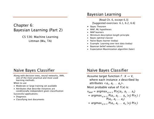
Chapter 6: Bayesian Learning (Part 2) Bayesian Learning Naïve ...

Chapter 6:
Bayesian Learning (Part 2)
CS 536: Machine Learning
Littman (Wu, TA)
Naïve Bayes Classifier
Along with decision trees, neural networks, kNN,
one of the most practical and most used
learning methods.
When to use:
• Moderate or large training set available
• Attributes that describe instances are
conditionally independent given classification
Successful applications:
• Diagnosis
• Classifying text documents
Bayesian Learning
[Read Ch. 6, except 6.3]
[Suggested exercises: 6.1, 6.2, 6.6]
• Bayes Theorem
• MAP, ML hypotheses
• MAP learners
• Minimum description length principle
• Bayes optimal classier
• Naïve Bayes learner (today)
• Example: Learning over text data (today)
• Bayesian belief networks (skim)
• Expectation Maximization algorithm (later)
Naïve Bayes Classifier
Assume target function f : X ! V,
where each instance x described by
attributes .
Most probable value of f (x) is:
v MAP = argmax vj in V P(v j|a 1, a 2 … a n)
= argmax vj in V P(a 1, a 2 … a n, |v j) P(v j ) /
P(a 1, a 2 … a n)
= argmax vj in V P(a 1, a 2 … a n, |v j) P(v j )

Naïve Bayes Assumption
P(a 1, a 2 … a n, |v j ) = # i P(a i |v j ),
which gives
Naïve Bayes classifier:
v NB = argmax vj in V P(v j ) # i P(a i |v j )
Note: No search in training!
Naïve Bayes: Example
• Consider PlayTennis again, and new
instance
Want to compute:
v NB = argmax vj in V P(v j) # i P(a i |v j)
P(y) P(sun|y) P(cool|y) P(high|y) P(strong|y) = .005
P(n) P(sun|n) P(cool|n) P(high|n) P(strong|n) = .021
• So, v NB = n
Naïve Bayes Algorithm
Naïve_Bayes_Learn(examples)
For each target value vj ^
P(v j) " estimate P(v j)
For each attribute value ai of each
attribute a
^
P(ai|vj) " estimate P(ai|vj) Classify_New_Instance(x)
^ ^
vNB = argmaxvj in V P(vj) # i P(ai |vj) Naïve Bayes: Subtleties
1. Conditional independence assumption is often
violated
P(a 1 , a 2 … a n, |v j ) = # i P(a i |v j )
• ...but it works surprisingly well anyway. Note
don't need estimated posteriors P(v j |x) to be
correct; need only that
argmax vj in V P(v j |a 1 , a 2 … a n )
= argmax vj in V P(v j ) # i P(a i |v j )
• Domingos & Pazzani [1996] for analysis
• Naïve Bayes posteriors often unrealistically
close to 1 or 0

Naïve Bayes: Subtleties
2. What if none of the training instances with
target value v j have attribute a i ?
P(a i |v j ) = 0, and… P(v j ) # i P(a i |v j ) = 0
Solution is Bayesian estimate:
P(a i |v j ) = (n c + mp)/(n + m) where
• n is number of training examples for which v = v j ,
• n c number of examples for which v = v j and a = a i
• p is prior estimate for P(a i |v j )
• m is weight given to prior (i.e., number of “virtual”
examples)
Learning to Classify Text
Target concept Interesting?: Document ! { +, - }
1. Represent each document by vector of words
• one attribute per word position in document
2. Learning: Use training examples to estimate
• P(+) P(-)
• P(doc| +) P(doc| -)
Learning to Classify Text
Why?
• Learn which news articles are of
interest
• Learn to classify web pages by
topic
Naïve Bayes is among most effective
algorithms
• What attributes shall we use to
represent text documents??
Naïve Bayes for Text
• Naïve Bayes conditional
independence assumption
P(doc |v j) = # i=1 length(doc) P(ai =w k|v j)
where P(a i =w k|v j) is probability that
word in position i is w k, given v j
One more assumption:
• P(a i =w k|v j) = P(a m =w k|v j) $i, m
“Bag of words” assumption.

Learning Algorithm
LEARN_NAÏVE_BAYES_TEXT(Examples, V )
1. collect all words and other tokens that occur in Examples
• Vocabulary " all distinct words and other tokens in
Examples
2. Calculate the required P(v j ) and P(w k |v j ) probability terms
• For each target value v j in V do
– docs j " subset of Examples for which the target value is v j
– P(v j ) " |docs j |/|Examples|
– Text j " a single document created by concatenating all
members of docs j
– n " total number of words in Text j (counting duplicate words
multiple times) (“tokens” vs. “tokens”)
– for each word w k in Vocabulary
• n k " number of times word w k occurs in Text j
• P(w k |v j ) " (n k + 1) / (n + |Vocabulary|)
Twenty NewsGroups
Given 1000 training documents from each
group, learn to classify new documents
according to newsgroup:
comp.graphics misc.forsale
comp.os.ms-windows.misc rec.autos
comp.sys.ibm.pc.hardware rec.motorcycles
comp.sys.mac.hardware rec.sport.baseball
comp.windows.x rec.sport.hockey
alt.atheism sci.space
soc.religion.christian sci.crypt
talk.religion.misc sci.electronics
talk.politics.mideast sci.med
talk.politics.misc talk.politics.guns
Naïve Bayes: 89% classification accuracy
Classification Algorithm
CLASSIFY_NAÏVE_BAYES_TEXT (Doc)
• positions " all word positions in
Doc that contain tokens found in
Vocabulary
• Return v NB, where
v NB = argmax vj in V P(v j) # i in positions P(a i|v j)
Article in rec.sport.hockey
• Path: cantaloupe.srv.cs.cmu.edu!das-news.harvard.edu
• From: xxx@yyy.zzz.edu (John Doe)
• Subject: Re: This year's biggest and worst (opinion)
• Date: 5 Apr 93 09:53:39 GMT
I can only comment on the Kings, but the most
obvious candidate for pleasant surprise is Alex
Zhitnik. He came highly touted as a defensive
defenseman, but he's clearly much more than that.
Great skater and hard shot (though wish he were more
accurate). In fact, he pretty much allowed the Kings
to trade away that huge defensive liability Paul
Coffey. Kelly Hrudey is only the biggest
disappointment if you thought he was any good to
begin with. But, at best, he's only a mediocre
goaltender. A better choice would be Tomas
Sandstrom, though not through any fault of his own,
but because some thugs in Toronto decided

Learning Curve
Accuracy vs. Training set size (1/3 withheld for test)
Conditional Independence
Definition: X is conditionally
independent of Y given Z if the
probability distribution governing X
is independent of the value of Y
given the value of Z; that is, if
($ x i, y j, z k) P(X = x i|Y = y j, Z = z k)
= P(X = x i|Z = z k)
more compactly, we write
P(X | Y, Z) = P(X | Z)
Bayesian Belief Networks
(Also called Bayes Nets, directed graphical
models, BNs, …). Interesting because:
• Naïve Bayes assumption of conditional
independence too restrictive
• But it's intractable without some such
assumptions...
• Belief networks describe conditional
independence among subsets of
variables
! allows combining prior knowledge about
(in)dependencies among variables with
observed training data
Independence Example
Example: Thunder is conditionally
independent of Storm, given Lightning
P(Thunder | Storm, Lightning)
= P(Thunder | Lightning)
Naïve Bayes uses conditional ind. to justify
P(X, Y | Z) = P(X |Y,Z) P(Y | Z)
= P(X |Z) P(Y | Z)

Bayesian Belief Network
Network represents a set of conditional ind. assertions:
• Each node is asserted to be conditionally ind. of its
nondescendants, given its immediate predecessors.
• Directed acyclic graph
Inference in Bayesian Nets
How can one infer the (probabilities of)
values of one or more network variables,
given observed values of others?
• Bayes net contains all information needed
for this inference
• If only one variable with unknown value,
easy to infer it
• Easy if BN is a “polytree”
• In general case, problem is NP hard (#Pcomplete,
Roth 1996).
Bayesian Belief Network
Represents joint probability distribution over all variables
• e.g., P(Storm, BusTourGroup, …, ForestFire)
• in general, P(y 1 ,…, y n ) = # i=1 n P(yi |Parents(Y i ))
where Parents(Y i ) denotes immediate predecessors of Y i in graph
• so, joint distribution is fully defined by graph, plus the
P(y i |Parents(Y i )) (CPTs)
Inference in Practice
In practice, can succeed in many cases
• Exact inference methods work well for
some network structures (small “induced
width”)
• Variational methods good approximation
if nodes tightly coupled
• Monte Carlo methods “simulate” the
network randomly to calculate
approximate solutions
Now used as a primitive in more advanced
learning and reasoning scenarios.

Learning of Bayesian Nets
Several variants of this learning task
• Network structure might be known
or unknown
• Training examples might provide
values of all network variables, or
just some
structure known unknown
observe
some all
like Naïve
Bayes
Gradient Ascent for BNs
Let w ijk denote one entry in the conditional
probability table for variable Y i in the
network
w ijk = P(Y i = y ij|Parents(Y i) = u ik values)
e.g., if Y i = Campfire, then u ik might be
Perform gradient ascent by repeatedly:
1. Update all w ijk using training data D
w ijk " w ijk + % & d in D P h(y ij, u ik|d)/w ijk
2. Then, renormalize the w ijk to assure
& j w ijk = 1, 0 ! w ijk ! 1
Learning Bayes Nets
Suppose structure known, variables
partially observable
e.g., observe ForestFire, Storm,
BusTourGroup, Thunder, but not
Lightning, Campfire...
Similar to training neural network with
hidden units
• In fact, can learn network conditional
probability tables using gradient ascent!
• Converge to network h that (locally)
maximizes P(D|h)
More on Learning BNs
EM algorithm can also be used.
Repeatedly:
1. Calculate probabilities of
unobserved variables, assuming h
2. Calculate new w ijk to maximize
E [ln P(D|h)]
where D now includes both observed
and (calculated probabilities of)
unobserved variables

Unknown Structure
When structure unknown...
• Algorithms use greedy search to
add/subtract edges and nodes
• Active research topic
Somewhat like decision trees:
searching for a discrete graph
structure
Expectation Maximization
When to use EM:
• Data is only partially observable
• Unsupervised clustering (target value
unobservable)
• Supervised learning (some instance
attributes or labels unobservable)
Some uses:
• Train Bayesian Belief Networks
• Unsupervised clustering (AUTOCLASS)
• Learning Hidden Markov Models
Summary: Belief Networks
• Combine prior knowledge with observed
data
• Impact of prior knowledge (when
correct!) is to lower the sample
complexity
• Active research area (UAI)
– Extend from Boolean to real-valued variables
– Parameterized distributions instead of tables
– Extend to first-order systems
– More effective inference methods
– ...
Mixtures of k Gaussians
Each instance x generated by
1. Choosing one of the k Gaussians with
uniform probability
2. Generating an instance at random according
to that Gaussian

EM for Estimating k Means
Given:
• Instances from X generated by mixture of
k Gaussian distributions
Not given:
• Means of the k Gaussians
• Which instance x i was generated by which
Gaussian
Determine:
• ML estimates of
EM for Estimating k Means
EM Algorithm: Pick random initial h = , then iterate
• E step: Calculate the expected value E[z ij]
of each hidden variable z ij, assuming the
current hypothesis h = holds.
• M step: Calculate a new maximum
likelihood hypothesis h’ = ,
assuming the value taken on by each
hidden variable z ij is its expected value
E[z ij] calculated above. Replace
h = by h’ = .
Missing Information
Think of full description of each
instance as y i = , where
• z ij is 1 if x i generated by j th
Gaussian (not observed)
• x i observed data value
If we had full instances, how estimate
µ 1, µ 2?
If we had µ 1, µ 2, how predict z ij?
E Step For k Means
E [z ij] = p(x=x i|µ=µ j) /
& n=1 2 p(x=xi|µ=µ n)
p(x=x i|µ=µ j) = exp(-1/(2' 2 )(x i - µ j) 2 )
Derived via PDF for Gaussians and
Bayes rule

M Step For k Means
µ j’ = (& n=1 m E [zij] x i) / (& n=1 m E [zij])
Estimates the mean by the sample
mean (average of the observed data
points, weighted by their probability
of being generated by the Gaussian
in question).
General EM Problem
Given:
• Observed data X = {x 1, … , x m }
• Unobserved data Z = {z 1, … , z m }
• Parameterized probability dist. P(Y | h),
where
– Y = {y 1, … , y m } is the full data y i = x i U z i
– h are the parameters
Determine:
• h that (locally) maximizes E [ln P(Y | h)]
EM Algorithm
Converges to local maximum likelihood h
and provides estimates of hidden
variables z ij
In fact, local maximum in E [ln P(Y | h)]
• Y is complete (observable plus
unobservable variables) data
• Expected value is taken over possible
values of unobserved variables in Y
General EM Method
Define likelihood function Q (h’, h),
which calculates Y = X U Z using
observed X and current parameters
h to estimate Z
Q (h’, h) " E [ln P(Y | h’) | h, X]

Abstract Algorithm
EM Algorithm:
Estimation (E) step: Calculate Q(h’, h)
using the current hypothesis h and the
observed data X to estimate the
probability distribution over Y .
Q(h’, h) " E [ln P(Y | h’) | h, X]
Maximization (M) step: Replace
hypothesis h by the hypothesis h’ that
maximizes this Q function.
h " argmax h’ Q(h’, h)