Numerical Simulation of a Cylinder in Uniform Flow: Application of a ...

JOURNAL OF COMPUTATIONAL PHYSICS 123, 450–465 (1996) 

ARTICLE NO. 0036 

Numerical Simulation of a Cylinder in Uniform Flow: Application of 

a Virtual Boundary Method 

E. M. SAIKI AND S. BIRINGEN 

Department of Aerospace Engineering Sciences, University of Colorado, Boulder, Colorado 

Received July 12, 1994; revised July 10, 1995 

In this study, a virtual boundary technique is applied to the numer- 

in its ability to model the material properties of the body 

and movement of the boundaries. However, numerical 

ical simulation of stationary and moving cylinders in uniform flow. stiffness of most moving boundary problems restricts the 

This approach readily allows the imposition of a no-slip boundary 

within the flow field by a feedback forcing term added to the momen- 

tum equations. In the present work, this technique is used with a 

high-order finite difference method, effectively eliminating spurious 

oscillations caused by the feedback forcing when used with spec- 

explicit definition of the forcing term in Peskin’s method 

to small time steps (Tu and Peskin [32]). This method has 

been expanded and implemented in a number of other 

problems modeling suspended particulates (Fogelson and 

trally discretized flow solvers. Very good agreement is found be- Peskin [12]) and the inner ear (Beyer [3]). 

tween the present calculations and previous computational and 

experimental results for steady and time-dependent flow at low 

Reynolds numbers. � 1996 Academic Press, Inc. 

In a related, yet independent, study, Goldstein et al. [15, 

16] developed a virtual boundary method based on the 

initial work of Sirovich [28, 29] which employs a forcing 

term governed by a feedback loop. Using a spectral 

INTRODUCTION 

method, they applied this procedure to investigate the effects 

of riblets on turbulent channel flow and to flow be- 

The fundamental fluid dynamics problem of a circular tween concentric cylinders. They noted that the forcing 

cylinder in uniform flow has been examined extensively function generated constant low amplitude, high frequency 

in both computational and experimental studies and is oscillations which they were able to control by numerical 

considered a stringent test for flow solvers. The difficulty low-pass filters and/or the introduction of particular flow 

which accompanies the computational approach to this fields inside of the body. Their simulations were not notice- 

problem by finite differences or spectral methods lies in ably affected by these spurious signals, but such numerical 

the representation of the cylinder geometry to allow for oscillations may become of concern when one calculates 

an accurate application of these numerical integration the evolution of a forced disturbance wave as in the simula- 

methods. The use of coordinate transformations and map- tion of flow instability and transition. 

ping techniques is possible but requires a highly accurate In the present study, we use the method developed by 

way of calculating the transformation Jacobians. Finite ele- Goldstein et al. [16] to simulate stationary, rotating, and 

ment methods (Gresho et al.[17]; Engelman and Jaminia oscillating cylinders in uniform flow at low Reynolds num- 

[11]; Karniadakis and Triantafyllou [21]) and conformal bers (Re � 400) allowing the assessment of the virtual 

transformations (Jordan and Fromm [20]; Braza et al. [4]; boundary technique to model a body in an unsteady flow 

Badr and Dennis [1]) have been successfully used for this field. In the present solution procedure, high-order finite 

problem. As an alternative to the use of generalized coordi- differences are implemented in order to suppress the nunates 

and coordinate transformations for finite difference merical oscillations caused by the forcing function ob- 

and spectral methods, Peskin [23] developed a method served in the Chebyshev spectral method of Goldstein et 

which represents a body within a flow field via a forcing 

term added to the governing equations. When applied at 

al. [16]. 

certain points in the flow, this forcing term simulates the 

effect of the body on the flow, allowing for the modeling 

COMPUTATIONAL METHOD 

of a boundary of any shape within a Cartesian computa- The numerical model integrates the two-dimensional, 

tional box without the necessity of mapping. Peskin [23, time-dependent, incompressible, Navier-Stokes, and con- 

24] successfully implemented this method (immersed tinuity equations nondimensionalized by the diameter of 

boundary technique) to model moving boundaries in heart the cylinder, D, and the free-stream velocity, U�,ona valve simulations. The main advantage of the scheme lies staggered mesh by a time-splitting method. The normal 

0021-9991/96 $18.00 

Copyright © 1996 by Academic Press, Inc. 

All rights of reproduction in any form reserved. 

450

VIRTUAL BOUNDARY METHOD 451 

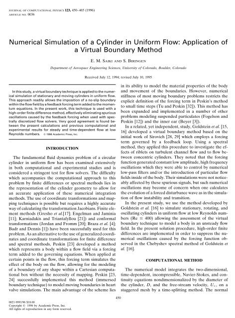
FIG. 1. Time distribution of the l 2-norm error in the no-slip condition imposed by the virtual boundary method defining a cylinder in uniform 

flow at Re � 25. Comparison between solutions with varying �/�: (a) over total run time; (b) closeup of first 1000 time steps; and (c) closeup of 

last 1000 time steps. � ��400000, � ��600, ———; � ��4000, � ��60, –––; � ��400, � ��6, –---–---. 

diffusion terms are advanced implicitly by the Crank– boundary, uniform flow conditions are assumed, i.e., u � 

Nicolson scheme and either the explicit third-order com- 1 and v � 0. At the outflow, boundary conditions are 

pact Runge–Kutta or Adams–Bashforth methods are prescribed to ensure that wave-like disturbances (gener- 

applied to the remaining terms (Streett and Hussaini ated by vortex shedding) in the high Reynolds number 

[30]). The equations are discretized spatially in the normal cases leave the computational domain without reflection. 

( y) and streamwise (x) directions by fourth-order central This was accomplished by appending a ‘‘buffer domain’’ 

finite differences. The pressure Poisson equation is evalu- to the physical domain (the length of the buffer domain 

ated by the tensor product method (Huser and Bir- was about 20–30% of the physical domain) in which the 

ingen [19]). governing equations were modified by reducing the stream- 

At the upper and lower boundaries, we impose shear wise viscous terms and the right-hand side of the pressure 

free conditions, i.e., �u/�y � 0 and v � 0 and at the inflow Poisson equation to zero at the outflow boundary using a

452 SAIKI AND BIRINGEN 

FIG. 2. Re � 550, t � 3: streamwise velocity. (a) Chebyshev; (b) finite differences. 

smooth coefficient function. Previous numerical experi- body moves, i.e., v � 0, then the position of the boundary 

ments have included rigorous testing of this technique, points at each time step is computed by integration of 

verifying its suitability for use in both high and low ampli- v � dxs/dt. The negative constants � and � are determined 

tude wave propagation problems (Streett and Macaraeg by observing the response of U once F is applied; � pro- 

[31]; Danabasoglu [9]; Danabasoglu et al. [10]; Saiki et duces the natural oscillation frequency of the response, 

al. [26]). while � dampens the oscillation of the response. For un- 

In implementing the method of Goldstein et al. [16] to steady flows, � must produce a response with a natural 

the present calculations of flow over a cylinder, the no- frequency greater than the highest frequencies present in 

slip boundary of the cylinder surface was represented by the flow so that F can respond correctly to the changing 

a feedback forcing function added to the momentum equa- flow field. The oscillatory nature of the boundary does not 

tions. This feedback function effectively brings the fluid affect the overall steady state of the flow field. However, 

velocity to zero at the desired points in the flow which for each combination of � and � a different forcing function 

define the no-slip boundary and can be expressed as is added to the right-hand side of the momentum equations, 

F(xs, t) � �� 

therefore a set of similar but slightly different flow fields 

are obtained for each of the solutions. For example, com- 

t 

0 (U(xs, t) � v(xs, t)) dt 

� �(U(xs, t) � v(xs, t)). 

(1) parison of the cylinder cases presented below revealed 

variations of 1–2% in the geometrical parameters of the 

wake. 

Here, F is the external force imposed at the discrete surface To examine the response of the virtual boundary to 

points defined by xs, and U is the fluid velocity at these different �/� combinations, a stationary cylinder at Re � 

surface points. The velocity of the body itself is controlled 25 was modeled and the l2-norm error of the velocities at 

by specifying v � (ub, vb) at the boundary points. If the the boundary points with respect to the no-slip boundary


FIG. 3. Re � 550: normal profiles of streamwise velocity in the vicinity of the cylinder. (a) x � 2.23750; (b) x � 2.2875; (c) x � 2.3125; 

(d) x � 2.3650. Chebyshev, ———; finite differences –––. 

condition was tracked in time. The l2-norm in the stream- The time step restricting this method is based upon the 

wise velocity is defined as 

values of � and � and the explicit time integration imple- 

mented in the flow solver. For the Adams–Bashforth 

method, Goldstein et al. [16] determined the following 

l 2-norm �� 1 

n b � n b 

i�1 

(u b) 2 i , (2) expression for the time step 

where nb is the number of virtual boundary points. The �t � �� (�2 results of this analysis are presented in Fig. 1. With the 

application of the higher values of these parameters, the 

� 2�k) 

, 

� 

(3) 

no-slip boundary condition is quickly attained. At the end where k is a problem dependent constant of order one. A 

of the time period considered, the l2-norm corresponding similar restriction was observed in the current study when 

to the lower �/� values is two orders of magnitude higher the Runge–Kutta method was used. 

than the other two cases; however, it continues to decay. In order to represent the body boundary in the flow 

These test cases suggest that higher values of the coeffi- field, Goldstein et al. [16] defined the boundary on 

cients allow the method to respond faster to any unsteadi- points which coincided with the computational grid nodes, 

ness in the flow field and act more efficiently in reinforcing whereas Peskin [23, 24] and Goldstein et al. [15] defined 

the no-slip conditions. These computations were con- the body boundary in a manner independent of the 

ducted using nb � 1441 boundary points; further increases computational grid. Peskin [23] utilized a first-order co- 

or decreases in nb with the same values of � and � yielded sine function to interpolate and extrapolate information 

similar results. between the immersed boundary and the grid. More


FIG. 4. Superposition of the virtual boundary points on the computa- 

tional grid: (a) full cylinder body; (b) upper left portion of the cylinder. 

recently, Beyer [3] developed a second-order accurate 

representation of the immersed boundary in applications 

of Peskin’s method. Goldstein et al. [15] implemented 

highly accurate spectral interpolation of the velocities 

from the grid points to the virtual boundary points and 

applied linear interpolation to distribute the effect of 

the forcing term to the grid nodes. 

In the current study, the fluid velocities are interpolated 

to a virtual boundary point, (xs, ys), from the four sur- 

rounding grid points denoted by the indices (i, j), 

(i � 1, j), (i, j � 1), and (i � 1, j � 1), using bilinear inter- 

polation, 

i�1, j�1 

U(xs) � � Di, j(xs)Ui, j, (4) 

i, j 

where 

In Eq. (5), 

and 

D i, j(x s) � d(x s � x i)d( y s � y j). (5) 

d(x s � x i) � (x s � x i�1) 

(x i � x i�1) 

d(x s � x i) � (x s � x i�1) 

(x i � x i�1) 

if x i � x s 

if x i � x s 

(6a) 

(6b) 

d(x s � x i) � 1 ifx i�x s. (6c) 

The effect of the virtual boundary force is extrapolated 

back to the grid points by area-weighted averages, 

F i, j � 1 

N b � N b 

n�1 

D i, j(x s)F n(x s), (7) 

where Nb is the number of virtual boundary points which 

affect the (i, j)th grid point. This method of spreading the 

boundary forces results in an effective boundary thickness 

on the order of one grid cell, i.e., O(�x, �y). The above 

interpolation/extrapolation scheme is first-order accurate, 

similar to the delta function representation of Peskin [23]. 

The low order accuracy of this operation influences mainly 

the flow field in the immediate vicinity of the cylinder; 

however, large scale features are successfully captured by 

this method. 

Both Peskin [23, 24] and Goldstein et al. [15, 16] imposed 

the forcing term only at points which defined the boundary, 

thus allowing fluid motion inside the body. For Peskin’s 

[23, 24] work this behavior is desirable since his calculations 

concern blood flow inside of the heart and the external 

flow field is ignored. Goldstein et al. [15, 16] investigated 

the effect of solid bodies placed within a flow field which 

physically do not permit flow inside the boundary. Conse- 

quently, the flow fields which were numerically allowed to 

develop in such boundaries were unphysical; however, the 

internal flow field was used as a smoothing device to attenu- 

ate spatial oscillations generated by the method (Goldstein 

et al. [15, 16]). In the present computations, some of the test 

cases (in particular, the Re � 550 case presented below) 

converged to an incorrect solution with the forcing term 

imposed only on the boundary. This behavior was remedied 

by imposing the forcing function inside the boundary 

of the body, as well as on the boundary. This suggests that 

in implementing the virtual boundary technique in solid 

body problems, where the solution is unknown, the forcing


FIG. 5. Re � 25: (a) spanwise vorticity, dotted and solid lines denote negative and positive levels, respectively; (b) streamfunction. 

term should be applied at the boundary and interior points the attenuation of the oscillations with the application of 

of the body in order to converge to a correct solution. finite differences. Comparison of the streamwise profiles 

In an earlier work by the authors [27], the virtual bound- in the normal direction (Fig. 3) provide clear evidence that 

ary technique was used with a different flow solver imple- the oscillations are strongly damped. 

menting Chebyshev polynomials in the wall-normal direction. 

Due to the global nature of the Chebyshev 

RESULTS 

polynomials, nongrowing, spatial oscillations in the normal 

and streamwise directions developed in the flow field when 

Stationary Cylinder in Uniform Flow 

the feedback forcing function was applied. The virtual The cases investigating uniform flow over a stationary 

boundary acts as a discontinuity in the spectral representa- cylinder examined Reynolds numbers (Re � U�D/�) rangtion 

of the flow field, thus causing the oscillations to arise ing from Re � 25 to Re � 400. The mesh resolution varied 

(Gibb’s phenomenon). These oscillations were similar to from 267 � 147 to 436 � 147 for computational domains 

those also observed by Goldstein et al. [16] and did not ranging from 20 � 10 to 34 � 10. As the Reynolds number 

appear to affect the flow field downstream of the body. In increased, the length of the computational domain was 

the present work, the application of a local discretization increased in order to accommodate the stronger vortices 

scheme, i.e., finite differences, in the normal direction dras- which were shed from the cylinder. These adjustments are 

tically reduced the amplitude of these spatial oscillations. reflected in the varying grid and domain sizes cited above. 

The effect of these different discretization methods (i.e., Mesh stretching was employed in both directions with grid 

the Chebyshev and finite difference methods) is illustrated clustering near the body: the minimum grid spacing in the 

in results obtained from computations of startup flow over vicinity of the cylinder for all cases was �xmin ��ymin � 

a cylinder at Re � 550 (Figs. 2 and 3). Contours of stream- 0.0375. The feedback forcing coefficients were set to � � 

wise velocity reveal the spatial oscillations which arise due �400000 and � ��600, and the number of points defining 

to the Chebyshev discretization (Fig. 2a), and Fig. 2b shows the cylinder was 1441. The distribution of points defining


FIG. 6. Re � 30 : (a) spanwise vorticity, dotted and solid lines denote negative and positive levels, respectively; (b) streamfunction. 

TABLE I 

Comparison of the Wake Properties behind a Stationary Cylinder with Experiments and Previous Computational Results 

for Re � 25 and Re � 30; Steady Flow Solutions 

Re � 25 Re � 30 

Coutanceau Coutanceau 

Properties of the wake behind a Present Gresho et al. & Bouard Clift et al. Present & Bouard Clift et al. 

stationary cylinder results [17] a [6] b [5] b results [6] b [5] b 

Length of the separation bubble (L) 1.41 1.15 1.22 — 1.7 1.53 — 

x-coordinate of the center of the 

vortex cores (a) 0.53 0.38 0.44 — 0.62 0.55 — 

y-distance between the vortex cores 

(b) 0.5 0.47 0.51 — 0.5625 0.54 — 

Minimum streamwise velocity on 

the axis of symmetry (u max) �0.064 �0.057 �0.057 — �0.08 �0.0743 — 

x-coordinate of minimum streamwise 

velocity on the axis of symmetry 

(d) 0.59 0.49 0.5 — 0.72 0.64 — 

Separation angle (�) 45� 45� 48� — 48� 50.1� — 

Drag coefficient (C d) 1.54 2.26 — 1.84 1.38 — 1.69 

a Computational study. 

b Experiment.


FIG. 7. Re � 50 : steady state solution. (a) spanwise vorticity, dotted and solid lines denote negative and positive levels, respectively; (b) streamfunction. 

the virtual boundary superimposed onto the computational At low Reynolds numbers, (4.5 � Re � 35), experiments 

grid is presented in Fig. 4. In this particular case, we chose reveal an attached, steady, symmetric, recirculating bubble 

to impose the virtual boundary only on points defining the which develops downstream of the cylinder (Coutanceau 

boundary of the cylinder; similar results were obtained and Defaye [7]). In the present simulations this behavior 

when points were imposed in the interior. The velocity is clearly observed in the stream-function and spanwise 

components of the boundary points, v, were set to zero. vorticity contours for Re � 25 and Re � 30, respectively 

FIG. 8. Re � 50 : unsteady solution. (a) spanwise voriticity, dotted and solid lines denote negative and positive levels, respectively; (b) streamfunction.


TABLE II 

Comparison of Quantitative Data with Results from Experiments and Previous Computational Studies; Unsteady Flow Solutions 

Drag coefficient: C d a Strouhal number: St Wavelength: � Vortex speed: St � 

Gresho Gresho Berger Gresho Gresho 

Present et al. Clift Present et al. Roshko & Wille Present et al. Present et al. 

Re results [17] b et al. [5] c results [17] b [26] c [2] c results [17] b results [17] b 

50 d 1.38 1.81 1.41 0.139 0.14 0.122 0.12–0.13 6.9 6.5 0.96 0.93 

65 1.33 — 1.33 0.152 — 0.143 — 6.3 — 0.96 — 

100 1.26 1.76 1.24 0.171 0.18 0.167 0.16–0.17 5.5 5.2 0.94 0.93 

200 1.18 1.76 1.16 0.197 0.21 — 0.18–0.19 4.7 4.4 0.93 0.92 

400 1.18 1.78 1.12 0.22 0.22 0.205 0.2–0.21 4.2 4.4 0.92 0.96 

a Drag coefficient is averaged in the unsteady cases. 

b Computational study. 

c Experiment. 

d Unsteady solution (Fig. 7). 

(Figs. 5 and 6). The physical parameters of the separation tions, the flow field was numerically perturbed. Similarly, 

bubble are compared with previous experimental and com- in the present study a perturbation was needed in order 

putational studies in Table I and show good agreement to obtain vortex shedding at Re � 50; however, the higher 

for both Reynolds numbers. 

Reynolds number cases did not require any external per- 

When the Reynolds number is increased to values in turbations. Consequently, Re � 50 is close to a critical 

the 35 � Re � 60 range, experiments observe asymmetry Reynolds number above which the solution becomes un- 

of the separation bubble and ‘‘wavy’’ behavior of the tail steady. It is possible that the steady state solution obtained 

of the wake. In the current computations it was found that for Re � 50 may eventually exhibit unsteadiness due to 

for Reynolds numbers in this range (in particular, Re � the buildup of truncation and machine errors in the solu- 

50) the type of wake behavior depends on whether the tion, but the computer time needed to arrive at this point 

initial conditions are perturbed. For example, if no forced would be considerable. 

perturbations are imposed a steady separation bubble de- According to experimental results, increasing the Reynvelops 

downstream of the cylinder (Fig. 7). The length of olds number beyond Re � 60 leads to the development 

the separation bubble in this case is L � 3 in agreement ofaKármán vortex street forced by vortices which are 

with the steady state computation of Fornberg [13] at shed alternately with a distinct frequency from the top and 

Re � 50. If the solution shown in Fig. 7 is disturbed by bottom of the cylinder (Coutanceau and Defaye [7]). In 

introducing a small perturbation in the flow field, vortex the present study, the formation of the vortex street is 

shedding is instigated. This behavior is demonstrated in depicted clearly in spanwise vorticity contours for Re � 

Fig. 8, where the cylinder was moved vertically 0.001 nondi- 65, 100, 200, and 400 (Fig. 9). In Fig. 10, vertical velocity 

mensional units away from its original position and then contours for Re � 400 are plotted, indicating a very smooth 

moved back, perturbing the flow field and generating a solution that is free of any detectable residual oscillations. 

Kármán vortex street. At Re � 50, Gresho et al. [17] also As the Reynolds number increases, the frequency of the 

observed vortex shedding from the cylinder with no shedding increases (Table II) and the vortices become 

attached separation bubble, and the wake characteristics more concentrated. The patterns obtained for Re � 65 

measured in the unsteady solution of the current study and Re � 100 show remarkable similarity to the flow visualshow 

good agreement compared with Gresho et al.’s [17] izations of Freymuth et al. [14]. The time spectra and signa- 

results (Table II). In the computational studies of Jordan ture of the streamwise velocity at a point downstream of 

and Fromm [20] and Braza et al. [4], no vortex shedding the cylinder reveals the presence of a spike at the vortex 

or asymmetry of the separation bubble was observed for street Strouhal number (St � U� f/D : f � dimensional 

Reynolds numbers up to 1000. Braza et al. [4] explained frequency); higher harmonics of the Strouhal number are 

this behavior by stating that the computational scheme also present (Fig. 11). Experiments predict that the onset 

was too ‘‘clean,’’ i.e., no external perturbations existed of three-dimensionality and turbulence will occur at Reyn- 

(as would appear in an experiment), therefore there was olds numbers below Re � 200 (Coutanceau and Defaye 

nothing to trigger any asymmetry or unsteadiness of the [7]). Because of the two-dimensional nature of the current 

flow field. To induce the vortex shedding in their simula- computations, turbulence and the effects of three-dimen-


FIG. 9. Spanwise vorticity; dotted and solid lines denote negative and positive levels, respectively. (a) Re � 65; (b) Re � 100; (c) Re � 200; 

(d) Re � 400. 

sionality cannot be obtained, however, the vortices shed Tables II and III summarize the drag coefficient (Cd), from the cylinder at Re � 200 and 400 exhibit some irregu- Strouhal number, the wave-length of the Kármán vortex 

larities associated with higher harmonics which subside as street (�), and the vortex speed (St �) observed for the 

the vortices are convected downstream, forming a laminar unsteady solutions and they provide comparisons with pre- 

Kármán vortex street (Figs. 9c–d). vious computational and experimental results. The Strou-


FIG. 10. Re � 400 : normal velocity, dotted and solid lines denote negative and positive levels, respectively. 

FIG. 11. Spectra and time signatures of streamwise velocity measured at (x d, y d) � 0.9445, �0.325); x d is the streamwise distance downstream 

from the cylinder and y d is the normal distance from the symmetry axis of the cylinder. (a) Re � 50 (unsteady solution, Fig. 7); (b) Re � 65; (c) 

Re � 100; (d) Re � 200; (e) Re � 400.


TABLE III the inflow boundary was too close to the cylinder or if the 

Comparison of Quantitative Data with Previous 

Computational Results for Re � 100; Unsteady Flow Solutions 

Gresho Engelman Braza Joran & 

domain was not wide enough, a higher Strouhal number 

was obtained. The distance between the inflow boundary 

and the cylinder in the current study (Li � 4) is comparable 

to the domain length used by Gresho et al. [17] and Engel- 

Present et al. & Jaminia et al. Fromm Karniadakis man and Jaminia [11], but shorter than those used by 

Re � 100 results [17] [11] [4] [20] et al. [21] Karniadakis and Triantafyllou [21], Braza et al. [4], and 

Cd St 

� 

St � 

1.26 

0.171 

5.5 

0.94 

1.76 

0.18 

5.2 

0.93 

1.411 

0.173 

5.32 

0.915 

1.28 

0.16 

— 

— 

1.28 

0.16 

— 

— 

— 

0.168 

— 

— 

Jordan and Fromm [20]. Accordingly, as shown in Table 

III, the Strouhal number obtained in the current computations 

falls within the range of Strouhal numbers determined 

by the previous computational studies. We performed several 

test calculations with an expanded computational domain 

which revealed a slight drop in Strouhal number 

(from 0.171 to 0.168 for Re � 100) confirming that the 

hal numbers obtained from the present results are slightly proximity of the boundaries affects the vortex-shedding 

higher than the experimental results; however, they corre- frequency. 

spond better than the values obtained by the majority In the present study the drag coefficient was calculated 

of the other computational studies. The higher Strouhal in a manner similar to Goldstein et al. [16]; the drag was 

number can be attributed to the size of the computational found by considering the loss of fluid momentum in the 

domain. Karniadakis and Triantafyllou [21] found that if domain, i.e., 

FIG. 12. Re � 200 : rotating cylinder. Time evolution of streamfunction contours. (a) t � 1; (b) t � 1.5; (c) t � 2; (d) t � 3; (e) t � 4; (f) t � 

5; (g) t � 5.5; (h) t � 6.


FIG. 12—Continued 

Cd � 2 � 

defined by the boundary points of the cylinder as � � 

� 

�� 

U 

�1 � 

Ui U 

dy. 

Ui� (8) tan�1 ( yb/xb). The characteristics of the startup flow at this Reynolds 

Due to the influence of the boundary conditions on the 

computation, Ui was defined as the maximum mean veloc- 

ity measured at a distance D/2 upstream of the cylinder. 

As Tables II and III reveal, good agreement is found for 

values of Cd, in comparison with experiments and previous 

computational work. 

number and rotation rate consist of a primary eddy evolving 

at the top of the cylinder and a developing second eddy below 

the x-axis of symmetry (Figs. 12a–d). The second eddy 

moves upward (Figs. 12c–d) inducing two secondary vortices 

which merge to form a single vortex at time, t � 6 (Figs. 

12e–h). The streamfunction contours obtained by the cur- 

rent study are in remarkable agreement with experimental 

Rotating Cylinder in Uniform Flow 

observations (Coutanceau and Ménard [8]) and previous 

computational results (Badr and Dennis [1]). Figure 13 

The startup flow over a cylinder rotating counterclock- demonstrates excellent comparison between profiles of 

wise in uniform flow was computed for Re � 200. The streamwise and normal velocity along the x-axis behind the 

rotation rate of the cylinder was � � 1, resulting in a cylinder obtained from the current computation and experi- 

tangential velocity of one half the freestream velocity mental measurements (Coutanceau and Ménard [8]). 

(vt � 0.5). The motion of the cylinder was introduced 

by setting the components of v in Eq. (6) to the proper 

Oscillating Cylinder in Uniform Flow 

streamwise and normal velocities arising from the rotation This computation was performed at Re � 200 with the 

of the cylinder, i.e., v � (�vt sin �, vt cos �), where � is 

cylinder oscillating parallel to the free-stream velocity at


FIG. 13. Re � 200 : rotating cylinder. Time evolution of the velocity profiles along the x-axis of symmetry. (a) streamwise velocity; (b) normal 

velocity. Current computational results: ----------. t � 1; –––, t � 1.5; –-–-–-, t � 2; –---–---, t � 3; ——, t � 4. Experimental results [8]: �, t � 1; 

*, t � 1.5; �, t � 2; �, t � 3; �, t � 4. 

a frequency, fc � 1.88 St, i.e., 1.88 times the Strouhal fre- the two clockwise vortices moving downstream alongside 

quency for the stationary cylinder. The amplitude of the the counterclockwise eddy. These results are in excellent 

oscillation resulted in a streamwise displacement of the agreement with experimental observations (Griffin and 

cylinder of �0.24, and the cylinder motion was prescribed 

by setting the horizontal velocities on the boundary points 

Ramberg [18]; Ongoren and Rockwell [22]). 

to ub � Ac cos(2�fct). The computations started with the 

cylinder stationary and oscillations were imposed once the 

CONCLUSION 

solution reached a quasi-steady state. In this study, we applied a virtual boundary method to 

For the parameters considered in the current study, several steady/unsteady flow problems. The method modthe 

vortex shedding pattern of the stationary case at els a no-slip boundary by an external forcing function 

Re � 200 (Fig. 9c) is modified by the oscillation of the added to the momentum equations. The computational 

cylinder. This clearly depicted in the time evolution of results for both stationary and moving cylinders in uniform 

spanwise vorticity contours over two oscillation periods flow compare favorably with both experimental and previ- 

of the cylinder (Fig. 14). During this time period an ous computational studies and lend further evidence to the 

antisymmetrical mode A � III (Ongoren and Rockwell applicability of the virtual boundary technique for steady 

[22]) appears consisting of two clockwise vortices shed and unsteady flow problems. The oscillations caused by 

from the top of the cylinder and the evolution of a the virtual boundary method when used with a spectral 

single counterclockwise eddy from the bottom. These discretization method were attenuated by the application 

vortices then form a vortex street with the weaker of 

of high-order finite differences.


FIG. 14. Re � 200 : oscillating cylinder. Time evolution of spanwise vorticity contours; dotted and solid lines denote negative and positive 

contours, respectively. (a) t � T/4; (b) t � T/2; (c) t � 3T/4; (d) t � T; (e) t � 5T/4; (f) t � 3T/2; (g) t � 7T/4; (h) t � 2T (T is the oscillation 

period of the cylinder).


ACKNOWLEDGMENTS 

Concentric Cylinders with an External Force Field,’’ in Proceedings, 

11th AIAA Computational Fluid Dynamices Conference, Orlando, 

This work was supported by the Navy under Grant DOD N00014-94- Florida, July 1993. 

1-0923. The authors thank James A. Fein for his continued interest in 16. D. Goldstein, R. Handler, and L. Sirovich, J. Comput. Phys. 105, 

this work. 

354 (1993). 

17. P. M. Gresho, R. Chan, C. Upson, and R. Lee, Int. J. Numer. Methods 

REFERENCES 

Fluids 4, 619 (1984). 

18. O. M. Griffin and S. E. Ramberg, J. Fluid Mech. 75(2), 31 (1976). 

1. H. M. Badr and S. C. R. Dennis, J. Fluid Mech. 158, 447 (1985). 19. A. Huser and S. Biringen, Int. J. Numer. Methods Fluids 14, 1087 

2. E. Berger and R. Wille, Annu. Rev. Fluid Mech. 4, 313 (1972). 

(1992). 

3. R. P. Beyer, J. Comput. Phys. 98, 145 (1992). 

20. S. K. Jordan and J. E. Fromm, Phys. Fluids 15, 371 (1972). 

4. M. Braza, P. Chassaing, and H. Ha Minh, J. Fluid Mech. 165, 79 (1986). 

21. G. E. Karniadakis and G. S. Triantafyllou, J. Fluid Mech. 238, 1 (1992). 

5. R. Clift, J. R. Grace, and M. E. Weber, Bubbles, Drops, and Particles 

(Academic Press, New York, 1978), p. 154. 

22. A. Ongoren and D. Rockwell, J. Fluid Mech. 191, 225 (1988). 

23. C. S. Peskin, J. Comput. Phys. 25, 252 (1977). 

6. M. Coutanceau and R. Bouard, J. Fluid Mech. 79(2), 231 (1977). 24. C. S. Peskin, Annu. Rev. Fluid Mech. 14, 235 (1982). 

7. M. Coutanceau and J. R. Defaye, Appl. Mech. Rev. 44, 255 (1991). 

25. A. Roshko, NACA Technical Note 2913, 1953 (unpublished). 

8. M. Coutanceau and C. Ménard, J. Fluid Mech. 158, 399 (1985). 

9. G. Danabasoglu, Ph.D. thesis, University of Colorado, 1992 (unpublished). 

10. G. Danabasoglu, S. Biringen, and C. L. Streett, Phys. Fluids A 3, 

2138 (1991). 

26. E. M. Saiki, S. Biringen, G. Danabasoglu, and C. L. Streett, J. Fluid 

Mech. 253, 485 (1993). 

27. E. M. Saiki and S. Biringen, ‘‘Numerical Simulation of Particle Effects 

on Boundary Layer Flow,’’ in Transition, Turbulence, and Combustion, 

Volume I: Transition edited by M. Y. Hussaini, T. B. Gatski, 

and T. L. Jackson (Kluwer Academic, Dordrecht, 1994, p. 267. 

11. M. S. Engelman and M. Jaminia, Int. J. Numer. Methods Fluids 11, 

985 (1990). 

28. L. Sirovich, Phys. Fluids 10, 24 (1967). 

29. L. Sirovich, Phys. Fluids 11, 1424 (1968). 

12. A. L. Fogelson and C. S. Peskin, J. Comput. Phys. 79, 50 (1988). 

30. C. L. Streett and M. Y. Hussaini, ICASE Report No. 86-59, 1986 (un- 

13. B. Fornberg, J. Fluid Mech. 98, 819 (1980). published). 

14. P. Freymuth, F. Finaish, and W. Bank, Phys. Fluids 29, 1321 (1986). 31. C. L. Streett and M. G. Macaraeg, Appl. Numer. Math. 6, 123 (1989). 

15. D. Goldstein, T. Adachi, and H. Sakata, ‘‘Modeling a Flow between 

32. C. Tu and C. S. Peskin, SIAM J. Sci. Stat. Comput. 13, 1361 (1992).

Numerical Simulation of a Cylinder in Uniform Flow: Application of a ...

Create successful ePaper yourself

Delete template?

Save as template?