DOTcvp: Dynamic Optimization Toolbox with Control Vector ...

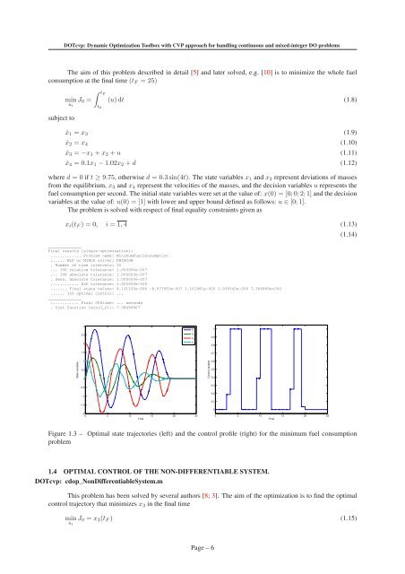
DOTcvp: Dynamic Optimization Toolbox with CVP approach for handling continuous and mixed-integer DO problemsThe aim of this problem described in detail [5] and later solved, e.g. [10] is to minimize the whole fuelconsumption at the final time(t F = 25)∫ tFminJ 0 = (u)dt (1.8)u i t 0subject toẋ 1 = x 3 (1.9)ẋ 2 = x 4 (1.10)ẋ 3 = −x 1 +x 2 +u (1.11)ẋ 4 = 0.1x 1 −1.02x 2 +d (1.12)where d = 0 if t ≥ 9.75, otherwise d = 0.3sin(4t). The state variables x 1 and x 2 represent deviations of massesfrom the equilibrium, x 3 and x 4 represent the velocities of the masses, and the decision variables u represents thefuel consumption per second. The initial state variables were set at the value of: x(0) = [0;0;2;1] and the decisionvariables at the value of: u(0) = [1] with lower and upper bound defined as follows: u ∈ [0;1].The problem is solved with respect of final equality constraints given asx i (t F ) = 0, i = 1,4 (1.13)______________Final results [single-optimization]:............. Problem name: MinimumFuelConsumption...... NLP or MINLP solver: FMINCON. Number of time intervals: 30... IVP relative tolerance: 1.000000e-007... IVP absolute tolerance: 1.000000e-007. Sens. absolute tolerance: 1.000000e-007............ NLP tolerance: 1.000000e-005....... Final state values: 8.131152e-006 -8.977053e-007 1.161981e-005 1.930543e-006 7.384969e+000...... 1th optimal control: ...______________............ Final CPUtime: ... seconds. Cost function [min(J_0)]: 7.38496867(1.14)32.52x 1x 2x 310.90.8x 40 5 10 15 20 251.50.7State variables10.50Control variable0.60.50.4−0.5−1−1.50.30.20.10−20 5 10 15 20 25TimeTimeFigure 1.3 – Optimal state trajectories (left) and the control profile (right) for the minimum fuel consumptionproblem1.4 OPTIMAL CONTROL OF THE NON-DIFFERENTIABLE SYSTEM.DOTcvp: cdop_NonDifferentiableSystem.mThis problem has been solved by several authors [8; 3]. The aim of the optimization is to find the optimalcontrol trajectory that minimizes x 3 in the final timeminu iJ 0 = x 3 (t F ) (1.15)Page – 6