Homopolar Generator Design Exercises - Kurt Nalty

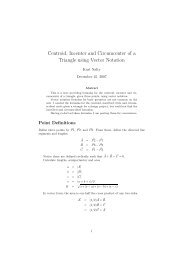
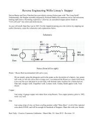
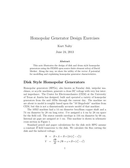
Homopolar Generator Design ExercisesKurt NaltyJune 24, 2013AbstractThis note illustrates the design of disk and drum style homopolargenerators using the FEMM open source finite element solver of DavidMeeker. Along the way, we show the utility of the vector ⃗ A potentialfor modelling and explaining homopolar generator characteristics.Disk Style Homopolar GeneratorsHomopolar generators (HPGs), also known as Faraday disk, unipolar machines,or acyclic machines, generate a clean DC voltage with very low internalimpedance. The Center for Electromechanics (CEM) at the Universityof Texas at Austin has designed, built and operated a variety of homopolargenerators from the mid 1970s through the current day. The machine weare about to model is roughly based upon the ”10 MegaJoule” machine fromCEM, but this is not a dimensionally accurate model of that machine.The 10MJ machine had a 14 cm diameter beryllium copper shaft and a74 cm diameter by 28 cm long rotor. I’ve assigned a 4 cm by 28 cm spacefor the field coil. The stator outside envelope is 116 cm diameter by 68 cm.Internal air gaps are assigned at 1 cm. This machine is shown in schematiccross section in Figure 1.Standard pencil and paper calculations for the disk style HPG assumea constant ⃗ B field transverse to the disk. We calculate the flux cutting thedisk and the induced voltage.Φ = B ∗ A = B ∗ (2π(r 2 o − r 2 i ))V = dΦdt ≈ fΦ = ω ∗ B ∗ (r2 o − r 2 i )1

Figure 1: Disk Style HPG with Cu Shaft and Field CoilFor this exercise, we will limit the rotor tip speed to 100 m/s (225 mph).We will also assume B = 1.5 T. We then have (given r = 37 cm.)v = rωω = v/r = 100m/s = 270 rad/s = 43 Hz = 2580 rpm0.37mV = ω ∗ B ∗ (ro 2 − ri 2 ) = 270 ∗ 1.5 ∗ (0.37 2 − 0.07 2 ) = 53V.To estimate the field coil requirements, we calculate the magnetic reluctanceof the HPG from the point of view of the field coil. We have an airgap of 2 cm, which I assume will dominate the magnetic circuit.R air =gµ 0 AΦ = NI/R airNI = ΦR air = (B ∗ A) ∗ gµ 0 A=1.5T ∗ 0.02mBg/µ 0 =1.26µH/m= 24 kA turns2

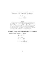
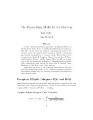
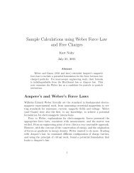
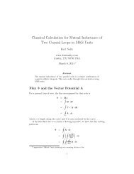
FEMM Model for Disk HPGThe source file for this model can be downloaded from http://www.kurtnalty.com/10MJ.fem. Step by step instructions for creating the simulation file areincluded at the end of this paper. After drawing, meshing and simulating,we have an axisymmetric contour map of flux shown in Figure 2. Using therainbow stripe widget, we can overlay a heat map of the magnitude of the Bfield, as shown in Figure 3.So, what does this tell us, and how is the information derived?For an axisymmetric configuration of currents and materials, the vectorpotential ⃗ A has zero radial and axial components. The only non-zero componentis A θ , and this is the item solved by the finite element method. Knowing⃗A, we can easily get flux and flux density. In the following equations, S is asurface area element, while s is linear path length element.⃗B = ∇∫ ⃗ ×∫A ⃗Φ = ⃗B · dS⃗=∫ ∫( ∇ ⃗ × A) ⃗ · dS⃗=∫⃗A · d⃗sΦ = 2πrA θRemembering that the generated voltage is V = fΦ, we see that thesecontours are also the voltage gradient along the rotor.V = fΦ= f2πrA θ= rωA θ= ⃗v · ⃗ARather than presenting the generator terms as dV = (⃗v × ⃗ B) · d⃗s, I preferto use the ⃗v · ⃗A.3

Figure 2: Contours of Constant Flux4

Figure 3: B Field and Flux Contours5

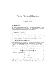
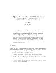
Unique Information from Finite Element SolutionSo, what information do we get from the finite element model that we didn’talready know from the pencil and paper calculations?As we look at the heatmap, we see that the rotor has a real voltagegradient (about 11%) along the outer surface. Current collection brushesshould be placed single file in the center plane of the rotor to reduce currentsin adjacent brushes in the z direction. Likewise, the low B in the center planeof the rotor reduces J ⃗ × B ⃗ forces on the current carrying brushes as well.We also notice at the inside radius of the stator near the rotor, that wehave a significant field concentration, and flux leakage into the shaft. Weshould radius this corner, increasing the local air gap, to reduce these fieldswhich may introduce currents into seals or bearing in this area. Otherwise,just make sure we don’t place bearings or seals in this location.The current collected on the outer rim needs to be evenly split, andtransported down the interior of the stator (becoming a compensating turn)to avoid high axial forces on the thrust bearing due to asymmetrical loading,and to reduce self inductance and armature reaction. Each shaft will haveset of brushes for the low voltage return, and a coaxial feed for the highervoltage from the rotor tip. External to the HPG will need to be a commonbus bonding these two halves together.Drum Style Homopolar GeneratorsThe drum style HPG shown here is guided by the Balcones Power Supply setof six HPGs at the Center for Electromechanics. For this design, we have twoseries connected, but oppositely wound field coils which drive flux radiallythrough the outer cylinder portion of the rotor.Figure 4 illustrates the drum style machine. Our design equation is thestandard physics formula V = B∗l∗v, where B is the magnetic field, typicallyaround 1.5 T, l is the active length of the rotor, and v is the tip velocity ofthe rotor. We use the principle of equal areas for flux transport to size theradius, length and stator back iron dimensions.FEMM Model for Drum HPGThe source file for this model can be downloaded from http://www.kurtnalty.com/Drum003.fem. The creation of the FEMM file for the drum HPGs fol-6

Figure 4: Drum HPG Geometry7

lows much the same sequence as the 10MJ file. The new feature is the twofield coils must be connected in series, but with the number of turns for thefirst coil a positive value (+1), while for the other coil, use a negative value(-1) for the number of turns.Looking at the flux map only (Figure 5), we see that assuming the shaftis at zero potential, the two output brushes on the extreme ends of the rotorare going to be at opposite polarities. For example, the outputs could be+25V and -25V with respect to the shaft.Now, let’s look at the combined flux and B map (Figure 6). For thisiteration, the position of the field coils has been adjusted to provide a lowflux location for the brush rings about a cm from the rotor edges. The outputof the collection brushes will come along the interior of the stator inside tothe midplane of the stator, and be brought out radially along equator. Noticethe use of radiusing to locally groom the airgap to reduce fringing fields inthe shaft.For this geometry, the formula V = Blv is certainly valid. However, theformula V = ⃗v · ⃗A also provides the correct voltage at each contour, as longas you keep in mind that A θ has opposite polarities in the upper versus lowermachine halves.8

Figure 5: Drum Contours of Constant Flux9

Figure 6: Drum Flux and B Field10

Step by Step Instructions for Creating the 10MJ.femFileI am using FEMM 4.2 for this project. Here is a step by step sequence tocreate the simulation file.Step by step for 10MJStart FEMMNew ProblemSelect "Magnetics Problem" OKProblem MenuAxisymetricUnits CentimetersComment - Practice HPGOKView->Keyboard (Set viewing area)Bottom -120Left 0Top 120Right 120OKPress NODE widget (Define centerline)tab r-coord 0 z-coord -120 OKtab r-coord 0 z-coord 0 OKtab r-coord 0 z-coord 120 OKPress LINE widget (Draw centerline)Single Click on bottom left (0,-120) nodeSingle Click on top right (0,120) nodeProperties -> Boundary (quasi-open space)Add PropertyName

Single Click on bottom left (0,-120) nodeSingle Click on top left (0,120) nodeArc Angle 180Max. segment 2.5 DegreesBoundary Condition Material Libraries (very bottom choice)Drag Air to right hand panelExpand Solid Non-Magnetic ConductorsDrag Copper to right hand panelShrink Solid Non-Magnetic ConductorsExpand Soft Magnetic MaterialsExpand Low Carbon SteelDrag 1020 Steel to right hand panelOK// Define shaftClick on NODE widgettab r-coord 0 z-coord 37 OKtab r-coord 7 z-coord 37 OKtab r-coord 7 z-coord -37 OKtab r-coord 0 z-coord -37 OKClick on LINE widgetclick on (0, 37) then click on (7, 37)click on (7, 37) then click on (7,-37)click on (7,-37) then click on (0,-37)click on (0,-37) then click on (0,37)Click on green BLOCK LABELS widgettab r-coord 3 z-coord 0 OKright click on (3,0). (Square will highlight red.)spacebarBlock type

Define rotorClick on NODE widgettab r-coord 7 z-coord -14 OKtab r-coord 37 z-coord -14 OKtab r-coord 37 z-coord 14 OKtab r-coord 7 z-coord 14 OKClick on LINE widgetclick on ( 7,-14) then click on (37,-14)click on (37,-14) then click on (37, 14)click on (37, 14) then click on ( 7, 14)click on ( 7, 14) then click on ( 7 -14)Click on green BLOCK LABELS widgettab r-coord 10 z-coord -10 OKright click on (10, -10). (Square will highlight red.)spacebarBlock type CircuitsAdd PropertyName

Click on LINE widgetclick on (40,-14) then click on (44,-14)click on (44,-14) then click on (44, 14)click on (44, 14) then click on (40, 14)click on (40, 14) then click on (40,-14)Click on green BLOCK LABELS widgettab r-coord 42 z-coord 0 OKright click on (42,0). (Square will highlight red.)spacebarBlock type

tab r-coord 32 z-coord -24 OKright click on (32, -24). (Square will highlight red.)spacebarBlock type