Iterated Register Coalescing - School of Computer Science

More documents

Recommendations

Info

Iterated Register Coalescing · 313—During simplify the degree of a node X might make the transition as a result ofremoving another node. Moves associated with neighbors of X are added to theworklistMoves.—When coalescing U and V, there may be a node X that interferes with both U andV. The degree of X is decremented, as it now interferes with the single coalescednode. Moves associated with neighbors of X are added. If X is move related, thenmoves associated with X itself are also added, as both U and V may have beensignificant-degree nodes.—When coalescing U to V, moves associated with U are added to the move worklist.This will catch other moves from U to V.7. BENCHMARKSFor our measurements we used seven Standard ML programs and SML/NJ compilerversion 108.3 running on a DEC Alpha. A short description of each benchmark isgiven in Figure 8. Five of the benchmarks use floating-point arithmetic—namely,nucleic, simple, format, andray.Some of the benchmarks consist of a single module, whereas others consist ofmultiple modules spread over multiple files. For benchmarks with multiple modules,we selected a module with a large number of live ranges. For the mlyaccbenchmarks we selected the modules defined in the files yacc.sml, utils.sml, andyacc.grm.sml.Each program was compiled to use six callee-save registers. This is an optimizationlevel that generates high register pressure and very many move instructions.Previous versions of SML/NJ used only three callee-save registers, because theircopy-propagation algorithms had not been able to handle six effectively.Figure 9 shows the characteristics of each benchmark. Statistics of the interferencegraph are separated into those associated with machine registers and thosewith pseudoregisters. Live ranges shows the number of nodes in the interferencegraph. For example, the knuth-bendix program mentions 15 machine registers and5360 pseudoregisters. These numbers are inflated as the algorithm is applied to allthe functions in the module at one time; in practice the functions would be appliedto connected components of the call graph. The average degree column, indicatingthe average length of adjacency lists, shows that the length of adjacencies associatedwith machine registers is orders of magnitude larger than those associatedwith pseudoregisters. The last two columns show the total number of move andnonmove instructions.8. RESULTSIdeally, we would like to compare our algorithm directly against Chaitin’s or Briggs’s.However, since our compiler uses many precolored nodes, and Chaitin’s and Brigg’salgorithms both do reckless coalescing (Chaitin’s more than Briggs’s), both of thesealgorithms would lead to uncolorable graphs.What we have done instead is choose the safe parts of Brigg’s algorithm—the early one-round conservative coalescing and the biased coloring—to compareagainst our algorithm. We omit from Brigg’s algorithm the reckless coalescing ofsame-tag splits.ACM Transactions on Programming Languages and Systems, Vol. 18, No. 3, May 1996, Pages 300-324.
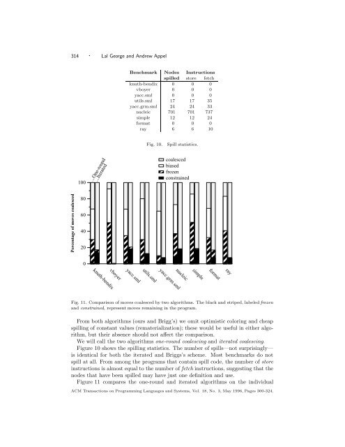
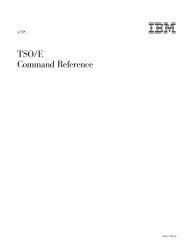
314 · Lal George and Andrew AppelBenchmark Nodes Instructionsspilled store fetchknuth-bendix 0 0 0vboyer 0 0 0yacc.sml 0 0 0utils.sml 17 17 35yacc.grm.sml 24 24 33nucleic 701 701 737simple 12 12 24format 0 0 0ray 6 6 10Fig. 10.Spill statistics.100...One-round...IteratedcoalescedbiasedfrozenconstrainedPercentage of moves coalesced806040200vboyerknuth-bendixyacc.smlutils.smlnucleicyacc.grm.smlsimpleformatrayFig. 11. Comparison of moves coalesced by two algorithms. The black and striped, labeled frozenand constrained, represent moves remaining in the program.From both algorithms (ours and Brigg’s) we omit optimistic coloring and cheapspilling of constant values (rematerialization); these would be useful in either algorithm,but their absence should not affect the comparison.We will call the two algorithms one-round coalescing and iterated coalescing.Figure 10 shows the spilling statistics. The number of spills—not surprisingly—is identical for both the iterated and Briggs’s scheme. Most benchmarks do notspill at all. From among the programs that contain spill code, the number of storeinstructions is almost equal to the number of fetch instructions, suggesting that thenodes that have been spilled may have just one definition and use.Figure 11 compares the one-round and iterated algorithms on the individualACM Transactions on Programming Languages and Systems, Vol. 18, No. 3, May 1996, Pages 300-324.
Page 1 and 2: Iterated Register CoalescingLAL GEO
Page 3 and 4: 302 · Lal George and Andrew Appelb
Page 5 and 6: 304 · Lal George and Andrew Appelf
Page 7: 306 · Lal George and Andrew AppelS
Page 11 and 12: 310 · Lal George and Andrew AppelT
Page 13: 312 · Lal George and Andrew AppelB
Page 17 and 18: 316 · Lal George and Andrew AppelF
Page 19 and 20: 318 · Lal George and Andrew AppelA
Page 21 and 22: 320 · Lal George and Andrew Appeld
Page 23 and 24: 322 · Lal George and Andrew Appelp
Page 25: 324 · Lal George and Andrew AppelC

Iterated Register Coalescing - School of Computer Science

You also want an ePaper? Increase the reach of your titles

Delete template?

Save as template?