Supply chain focus dependent supplier selection problem

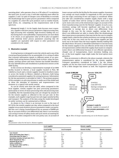
G. Vanteddu et al. / Int. J. Production Economics 129 (2011) 204–216 213warming plate’, who operates close to a CIR value of 1 to minimizethe total costs. In such a case, it will take relatively more effort forsuppliers 2 and 3 in spite of cheaper costs of flexibility to overtakethe disadvantage due to poor process parameters when comparedto a supplier of a short life cycle products such as mother boards,hard drives, etc. competing on the responsiveness end of thespectrum.Managerial insight 2: As the Supply chain becomes more responsive,suppliers with poor process parameters (high processing time,high processing time variability, high inventory holding rate etc)but having lower costs of flexibility (responsiveness) are more likelyto be chosen, at an appropriate value of CIR in place of supplierswith relatively better process parameters assuming that thesuppliers are equivalent with respect to other parameters notconsidered in the model.5. Illustrative exampleA wiring harness is designed to wire the vehicle and is one of thecrucial purchased products for an automobile. It is a string of cablesthat transmit information signals to different points in an automobile.Each wiring harness includes built-in fuses, relays for fans,pumps, auxiliary power and more. Harness has bundle identifiersfor easy identification and installation to production sensors at theOEM facility.In this section we develop a representative example of an OEMfacility located in Detroit, a local supplier located in Flint, MI(labeled as local) and a remote supplier located in Southern statesor across the border in Mexico (labeled as Remote), both beingconsidered as potential suppliers for wiring harnesses. Informationfor the key parameters is provided in Table 5. The primary purposeof this example is to aid a practitioner to make use of the model andto show the interplay of inventory and responsiveness costelements in a typical real-world context.As can be clearly seen from the table, when compared to thelocal supplier, remote supplier has poor processing parametersparticularly in terms of mean processing time and processing timevariability. But the manufacturing costs are cheaper by around 2%for the remote supplier as reflected in the cost per unit. In thisexample, each supplier stage has got two sub stages namely facilityand transport. The analysis of the data using the model developedin earlier sections can be summarized as follows.As shown in Fig. 4 there is an increase in cost to the tune of$2134 for the remote supplier per day, when compared to the localsupplier on account of poorer process parameters under cost parity.But this cost is being counterbalanced by an amount of $4000 perday on account of direct cost differential and, there is an inventorycost saving in terms of safety stocks and cycle stocks accounting for$82 per day, when compared to the cost parity case, on account oflower cost per unit for the facility for the remote supplier. Inventorycost savings are much smaller in magnitude in this case becausejust one stage (consisting of two sub stages) is considered. Whenyou take into consideration complex supply chains with a largenumber of nodes there will be savings in safety stock costs andcycle stock costs even at the downstream stages on account of thelower manufacturing costs for the ‘Remote’ supplier. In such a case,inventory savings will become significant and may even becomparable to savings due to direct cost differential. Eventhough in this case, for the remote supplier, savings due todirect cost differential are able to clearly offset the disadvantagedue to poor process parameters that may not be the case in complexsupply chains, wherein the echelon inventory cost savings also playa key role. In this case, total cost for the remote supplier per dayturns out to be lower than the local supplier thereby making himthe ideal choice. Of course, it should be noted that it is not necessaryfor the remote supplier to be cost effective all the time in the bandof responsiveness within which the supply chain wants to compete.Lower direct cost differential because of cost efficient operations,cheaper cost of transportation, lower inventory holding cost,etc. at the local supplier stage might make the local option moreattractive.Now an extension is offered to the above example, wherein theresponsiveness option is considered for the remote supplier.Transport parameters considered in Table 5 for the remotesupplier are for less than truck transportation (LTL), which tendsto be a little cheaper but slower as well. The responsive optionLocal: $ 208,205$ 4,000Savingsdue to costdifferentialRemoteSupplierRemote: $206,258$ 2,134$ 82InventoryCost (SS+CS)Savings compared toCost parity caseIncrease in costs forRemote supplier on account ofpoor process parameters undercost parityFig. 4. Effect of cheaper manufacturing cost on the Remote supplier.Table 5Key parameter values for the local vs. Remote suppliers.Local supplierRemote supplierLocal facility Local transport Remote facility Remote transportCost ($)/unit 256 4 243 12Mean processing time (days) L j 1 0.25 3 11Processing time SD (days) s j 0.25 0.1 1 2Inventory carrying cost per year (%) h j 24 24 24 24Mean demand per day m 800 800 800 800Demand SD per day s 150 150 150 150Safety coefficient k j 1.28 1.28 1.28 1.28Average back order coeff & p j 0.1 0.1 0.1 0.1F(k j ) Service level 0.9 0.9 0.9 0.9